Heavy Traffic Limits for GI/H/n Queues: Theory and Application Yousi Zheng * , Ness B. Shroff *+ , and Prasun Sinha + * Department of Electrical and Computer Engineering, + Department of Computer Science and Engineering, The Ohio State University, Columbus, Ohio 43210, USA August 1, 2012 Abstract We consider a GI/H/n queueing system. In this system, there are multiple servers in the queue. The inter-arrival time is general and independent, and the service time follows hyper-exponential distribu- tion. Instead of stochastic differential equations, we propose two heavy traffic limits for this system, which can be easily applied in practical systems. In applications, we show how to use these heavy traffic lim- its to design a power efficient cloud computing environment based on different QoS requirements. 1 Introduction Many large queueing systems, like call centers and data centers, contain thousands of servers. For call centers, it is common to have 500 servers in one call center [1]. For data centers, Google has more than 45 data centers 1

Welcome message from author
This document is posted to help you gain knowledge. Please leave a comment to let me know what you think about it! Share it to your friends and learn new things together.
Transcript
Heavy Traffic Limits for GI/H/n Queues: Theory
and Application
Yousi Zheng*, Ness B. Shroff*+, and Prasun Sinha+
*Department of Electrical and Computer Engineering,
+Department of Computer Science and Engineering,
The Ohio State University, Columbus, Ohio 43210, USA
August 1, 2012
Abstract
We consider a GI/H/n queueing system. In this system, there are
multiple servers in the queue. The inter-arrival time is general and
independent, and the service time follows hyper-exponential distribu-
tion. Instead of stochastic differential equations, we propose two heavy
traffic limits for this system, which can be easily applied in practical
systems. In applications, we show how to use these heavy traffic lim-
its to design a power efficient cloud computing environment based on
different QoS requirements.
1 Introduction
Many large queueing systems, like call centers and data centers, contain
thousands of servers. For call centers, it is common to have 500 servers in
one call center [1]. For data centers, Google has more than 45 data centers
1
2
as of 2009, and each of them contains more than 1000 machines [2]. When
the number of servers goes to infinity, many queueing systems should be
stable as long as the traffic intensity ρn < 1 (i.e., the arrival rate is smaller
than the service capacity). The traffic intensity for a queueing system with
n servers can be thought of as the rate of job arrivals divided by the rate
at which jobs are serviced. At the same time, the queueing systems should
work efficiently, which means that ρn should approach 1, i.e., limn→∞
ρn = 1.
This regime of operation is called the heavy traffic regime. Our paper focuses
on establishing heavy traffic limits, and using these limits to design a power
efficient cloud based on different QoS requirements.
Some classical results on heavy traffic limits are given by Iglehart in [3],
Halfin and Whitt in [4], and summarized by Whitt in Chapter 5 of his recent
book [5]. This heavy traffic limit ((1−ρn)√n goes to a constant as n goes to
infinity) is now called the Halfin-Whitt regime. Recently, the behavior of the
normalized queue length in this regime has been studied by A. A. Puhalskii
and M. I. Reiman [6], J. Reed [7], D. Gamarnik and P. Momeilovic [8], and
Ward Whitt [9,10]. Based on these studies, some design and control policies
are proposed in [11–14].
Our work differs from prior work in three key aspects. First, literature
on heavy traffic limits that is based on analysis of call center systems does
not capture various unique features of large queueing systems today, such as
the cloud computing environment. Many of those works assume a Poisson
arrival process and exponential service time [11–14]. Perhaps appropriate
for smaller systems, these models need to be generalized for today’s larger
systems such as increasingly complex call-centers and cloud computing en-
vironments. The arrival process in such complex and large systems may
be independent, but more general. More importantly, the service times of
3
jobs are quite varied and unlikely to be accurately modeled by an expo-
nential service time distribution. In [9], Whitt also considers the hyper-
exponential distributed service time, but only with two stages and where
one of them always has zero mean. Second, although some QoS metrics
(especially Quality-Efficiency-Driven (QED)) have been extensively studied
in some call center scenarios [11,12,15], the QoS requests can be more com-
plex, because of the wide variety of application needs, especially in the cloud
computing environment [16–18]. And third, while there are studies that give
heavy traffic solutions for more general scenarios [6, 7], these solutions can
only be described by complex stochastic differential equations, which are
quite cumbersome to use and provide little insight.
In this paper, we build a system model for general and independent inter-
arrival process and hyper-exponentially distributed service times. As men-
tioned earlier, the general arrival process can be used to characterize a vari-
ety of arrival distributions for the queueing system. The main motivation for
studying the hyper-exponential distribution is that it can capture the high
degree of variability in the service time. For example, the hyper-exponential
distribution can characterize any coefficient of variation (standard devia-
tion divided by the mean) greater than 1. Since the service time of jobs
is expected to be highly variable from job to job, the hyper-exponential
distribution is well suited to model the service times for today’s queueing
systems.
To satisfy the QoS and save operation cost at the same time, we char-
acterize the performance of the queueing system for four different types
of QoS requirements: Zero-Waiting-Time (ZWT), Minimal-Waiting-Time
(MWT), Bounded-Waiting-Time (BWT) and Probabilistic-Waiting-Time
(PWT) (the precise definitions are given in Section 2). Since the heavy
4
traffic limits for the ZWT and PWT classes can be directly derived from
the current literature (details in our technical report [19]), we simply list
their results, and focus instead on the MWT and BWT classes for which we
develop new heavy traffic limits. We use the heavy traffic limits to character-
ize the relationship between the traffic intensity and the number of servers
in the queueing systems.
In applications, we show how to use these heavy traffic limit results to
determine the number of active machines in a cloud to ensure that the QoS
requirements are met and the cloud operates in a stable and cost efficient
manner. Cloud computing environments are rapidly deployed by the in-
dustry as a means to provide efficient computing resources. A significant
fraction of the overall cost of operating a cloud is the amount of power it
consumes, which is related to the number of machines in operation. In order
to efficiently manage the power cost associated with cloud computing, we
develop the foundations for designing a cloud computing environment. In
particular, we aim to determine how many machines a cloud should have
to sustain a specific system load and a certain level of QoS, or equivalently
how many machines should be kept awake at any given time. Finally, using
simulations we show that depending on the QoS requirements of the cloud,
the cloud needs substantially different number of machines. We also show
that the number of operational machines in simulations are consistent with
the proposed design based on the new set of heavy traffic limit results. Al-
though the number of operational machines is derived from heavy traffic
limits, simulation results indicate that it is a good methodology, even when
the number of machines is finite, but large.
The main contributions of this paper are:
• This paper makes new contributions to heavy traffic analysis, in that it
5
derives new heavy traffic limits for two important QoS classes (MWT
and BWT) for queueing systems when the arrival process is general
and the service times are hyper-exponentially distributed.
• Using the heavy traffic limits results, this paper answers the important
question for enabling a power efficient cloud computing environment
as an application: How many machines should a cloud have to sustain
a specific system load and a certain level of QoS, or equivalently how
many machines should be kept awake at any given time?
The paper is organized as follows. In Section 2, we present the system
model of the queueing system, and describe the four different classes of QoS
requirements. Based on this model, we develop heavy traffic limits results
in Section 3 and Section 4 for the MWT and BWT classes correspondingly.
Using these heavy traffic limits results and the results in our technical report
[19], in Section 5 we consider cloud computing environment as an application
and compute the operational number of machines needed for different classes
of clouds. Simulation results are also provided in Section 6. Finally, we
conclude this paper in Section 7.
2 System Model and QoS Classes
2.1 System Model and Preliminaries
We assume that the queueing system consists of a large number of servers,
out of which n are active/operational at any given time. A larger n will
result in better QoS at the expense of higher operational cost.
We assume that the job arrivals to the system are independent with rate
λn and coefficient of variation c.
6
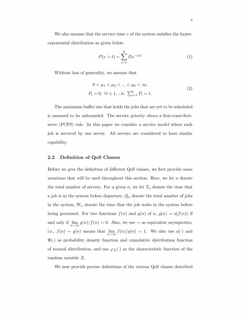
We also assume that the service time v of the system satisfies the hyper-
exponential distribution as given below.
P (v > t) =
k∑
i=1
Pie−µit (1)
Without loss of generality, we assume that
0 < µ1 < µ2 < ... < µk <∞;
Pi > 0, ∀i ∈ 1, ...k;∑k
i=1 Pi = 1.(2)
The maximum buffer size that holds the jobs that are yet to be scheduled
is assumed to be unbounded. The service priority obeys a first-come-first-
serve (FCFS) rule. In this paper we consider a service model where each
job is serviced by one server. All servers are considered to have similar
capability.
2.2 Definition of QoS Classes
Before we give the definition of different QoS classes, we first provide some
notations that will be used throughout this section. Here, we let n denote
the total number of servers. For a given n, we let Tn denote the time that
a job is in the system before departure, Qn denote the total number of jobs
in the system, Wn denote the time that the job waits in the system before
being processed. For two functions f(n) and g(n) of n, g(n) = o(f(n)) if
and only if limn→∞
g(n)/f(n) = 0. Also, we use ∼ as equivalent asymptotics,
i.e., f(n) ∼ g(n) means that limn→∞
f(n)/g(n) = 1. We also use φ(·) and
Φ(·) as probability density function and cumulative distribution function
of normal distribution, and use ϕX(·) as the characteristic function of the
random variable X.
We now provide precise definitions of the various QoS classes described
7
in the introduction. Since we are interested in studying the performance of
the system in the heavy traffic limit, we let the traffic intensity ρ → 1 as
n→ ∞ in the case of each QoS class we study.
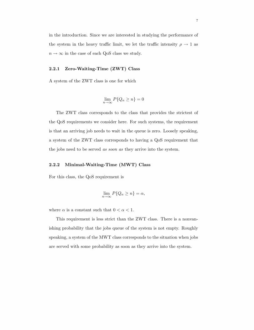
2.2.1 Zero-Waiting-Time (ZWT) Class
A system of the ZWT class is one for which
limn→∞
PQn ≥ n = 0
The ZWT class corresponds to the class that provides the strictest of
the QoS requirements we consider here. For such systems, the requirement
is that an arriving job needs to wait in the queue is zero. Loosely speaking,
a system of the ZWT class corresponds to having a QoS requirement that
the jobs need to be served as soon as they arrive into the system.
2.2.2 Minimal-Waiting-Time (MWT) Class
For this class, the QoS requirement is
limn→∞
PQn ≥ n = α,
where α is a constant such that 0 < α < 1.
This requirement is less strict than the ZWT class. There is a nonvan-
ishing probability that the jobs queue of the system is not empty. Roughly
speaking, a system of the MWT class corresponds to the situation when jobs
are served with some probability as soon as they arrive into the system.
8
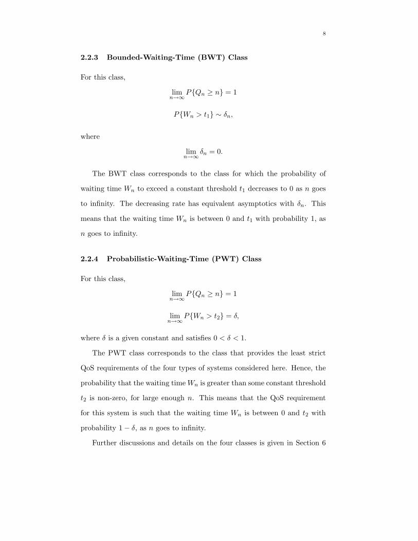
2.2.3 Bounded-Waiting-Time (BWT) Class
For this class,
limn→∞
PQn ≥ n = 1
PWn > t1 ∼ δn,
where
limn→∞
δn = 0.
The BWT class corresponds to the class for which the probability of
waiting time Wn to exceed a constant threshold t1 decreases to 0 as n goes
to infinity. The decreasing rate has equivalent asymptotics with δn. This
means that the waiting time Wn is between 0 and t1 with probability 1, as
n goes to infinity.
2.2.4 Probabilistic-Waiting-Time (PWT) Class
For this class,
limn→∞
PQn ≥ n = 1
limn→∞
PWn > t2 = δ,
where δ is a given constant and satisfies 0 < δ < 1.
The PWT class corresponds to the class that provides the least strict
QoS requirements of the four types of systems considered here. Hence, the
probability that the waiting timeWn is greater than some constant threshold
t2 is non-zero, for large enough n. This means that the QoS requirement
for this system is such that the waiting time Wn is between 0 and t2 with
probability 1 − δ, as n goes to infinity.
Further discussions and details on the four classes is given in Section 6
9
and our technical report [19]. For the rest of the paper, we will mainly focus
on developing new heavy traffic limits for the MWT and BWT classes.
3 Heavy Traffic Limit Analysis for the MWT class
The following result tells us how the number of servers must scale in the
heavy traffic limit for the MWT class.
Proposition 1. Assume
limn→∞
ρn = 1, (3)
limn→∞
PQn ≥ n = α, (4)
then
L ≤ limn→∞
(1 − ρn)√n ≤ U, (5)
where
U =
(k∑
i=1
β(i)U
√Piµi
)õ, (6)
L = maxi∈1,...k
β
(i)L
√Piµi
õ, (7)
µ =
(k∑
i=0
Piµi
)−1
, ρn =λnnµ
, (8)
β(i)U = (1 + c2−1
2 Pi)ψU ,
αk
= [1 +√
2πψUΦ(ψU ) exp (ψ2U/2)]
−1,(9)
β(i)L = (1 + c2−1
2 Pi)ψL,
α = [1 +√
2πψLΦ(ψL) exp (ψ2L/2)]
−1,(10)
10
0 ≤ α ≤ 1, 0 ≤ βL ≤ ∞, 0 ≤ βU ≤ ∞. (11)
In Proposition 1, ψU is the solution of Eq. (9), and β(i)U can be computed
using ψU . Similarly, ψL is the solution of Eq. (10), and β(i)L can be computed
using ψL. Thus, upper bound U in Eq. (6) and lower bound L in Eq. (7)
can be achieved using β(i)U , β
(i)L , and other parameters.
To prove Proposition 1, we construct an artificial system structure. The
arrival process and the capacity of a single server are same as the original
system. In the artificial system, we assume that there are k types of jobs.
For each arrival, we know the probability of ith type job is Pi, and the ser-
vice time of each ith type job is exponentially distributed with mean 1/µi.
Thus, the service time v of the system can be viewed as a hyper-exponential
distribution which satisfies Eq. (1). We also assume that there is an omni-
scient scheduler for the artificial system. This scheduler can recognize the
type of arriving jobs, and send them to the corresponding queue. For ar-
rivals of type i, the scheduler sends them to the ith queue, which contains ni
servers. Then the arrival rate of the ith queue is Piλn. Also, the priority of
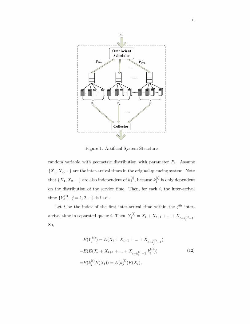
each separated queue obeys the FCFS rule. The artificial system is shown
in Fig. 1.
Lemma 2. For the ith separated queue, the inter-arrival time Y (i)j , j =
1, 2, ... is i.i.d., and the coefficient of variance c(i) =√
1 + (c2 − 1)Pi.
Proof. For the ith separated queue in Fig. 1, the inter-arrival time Y (i) is a
summation of inter-arrival times of a certain number of consecutive arrivals
in the original queue. The number of the summands is a random variable
k(i)j . k
(i)j is equal to the number of original arrivals between (j − 1)th and
jth arrivals in the ith separated queue.
Based on the structure of the artificial system, k(i)j is an independent
11
Figure 1: Artificial System Structure
random variable with geometric distribution with parameter Pi. Assume
X1,X2, ... are the inter-arrival times in the original queueing system. Note
that X1,X2, ... are also independent of k(i)j , because k
(i)j is only dependent
on the distribution of the service time. Then, for each i, the inter-arrival
time Y (i)j , j = 1, 2, ... is i.i.d..
Let t be the index of the first inter-arrival time within the jth inter-
arrival time in separated queue i. Then, Y(i)j = Xt +Xt+1 + ...+X
t+k(i)j −1
.
So,
E(Y(i)j ) = E(Xt +Xt+1 + ...+X
t+k(i)j −1
)
=E(E(Xt +Xt+1 + ...+Xt+k
(i)j −1
|k(i)j ))
=E(k(i)j E(Xt)) = E(k
(i)j )E(Xt),
(12)
12
and
V ar(Y(i)j ) = E
((Y
(i)j )2
)−(E(Y
(i)j ))2
=E
((Xt +Xt+1 + ...+X
t+k(i)j −1
)2)−(E(Y
(i)j ))2
=E(E
((Xt +Xt+1 + ...+X
t+k(i)j −1
)2|k(i)j
)) −
(E(Y
(i)j ))2
=E(E(X2t +X2
t+1 + ...+X2
t+k(i)j −1
+
2XtXt+1 + ...+ 2Xt+k
(i)j −2
Xt+k
(i)j −1
|k(i)j )) −
(E(Y
(i)j ))2
=E((k
(i)j )2(E(Xt))
2 + k(i)j V ar(Xt)
)−(E(Y
(i)j ))2
=E((k(i)j )2)(E(Xt))
2 + E(k(i)j )V ar(Xt) − E(k
(i)j )2E(Xt)
2
=V ar(k(i)j )E(Xt)
2 + E(k(i)j )V ar(Xt).
(13)
Thus, we can achieve the coefficient of variation c(i) for all the separated
queues as below.
c(i) =
√V ar(Y
(i)j )/
(E(Y
(i)j ))2
=
√V ar(ki) (E(Xt))
2 + E(ki)V ar(Xt)
E(ki)2E(Xt)2
=
√√√√1−Pi
P 2i
E(Xt)2 + 1PiV ar(Xt)
1P 2
i
E(Xt)2=√
1 + (c2 − 1)Pi.
(14)
Remark 3. If the arrival process is Poisson, c = 1, then c(i) = 1, ∀i =
1, 2, ...k. If the arrival process is deterministic, c = 0, then the inter-
arrival time of each separated queue has a geometric distribution, and c(i) =√
1 − Pi, ∀i = 1, 2, ...k.
Proof of Proposition 1. To prove this proposition, we must prove both the
upper and the lower bounds of the limit. For the upper bound, we consider
13
the Artificial System I, which satisfies the following condition:
limni→∞
(1 − ρni)√ni = β
(i)U , (15)
where
ρni=Piλnniµi
,
β(i)U =
(1 + (c(i))2)ψU2
= (1 +c2 − 1
2Pi)ψU ,
(16)
and
α
k= [1 +
√2πψUΦ(ψU ) exp (ψ2
U/2)]−1. (17)
The result of Theorem 4 in [4] shows that
limn→∞
PQn ≥ n = αc (18)
if and only if
limn→∞
(1 − ρn)√n = β, (19)
under the following conditions:
β = (1+c2)ψ2 ,
αc = [1 +√
2πψΦ(ψ) exp (ψ2/2)]−1,
0 ≤ αc ≤ 1, 0 ≤ β ≤ ∞.
(20)
By applying this result into Artificial System I, for each individual queue,
we have
limni→∞
PQ(i)ni
≥ ni =1
k, ∀i ∈ 1, ...k, (21)
where Q(i)ni is the length of the ith separated queue.
14
Let nU =∑k
i=1 ni, QnU=∑k
i=1Q(i)ni . Then, for Artificial System I, we
have
PQnU≥ nU = P
k∑
i=1
Q(i)nU
≥k∑
i=1
ni
≤P(
k⋃
i=1
Q(i)ni
≥ ni)
≤k∑
i=1
PQ(i)ni
≥ ni.(22)
By taking the limit on both sides,
limni→∞i∈1,...k
PQnU≥ nU
≤ limni→∞i∈1,...k
(k∑
i=1
PQ(i)ni
≥ ni)
=
(k∑
i=1
limni→∞
PQ(i)ni
≥ ni)
= α
(23)
From Eq. (23), we know that when Artificial System I has nU servers,
the probability that queue length QnUis greater than or equal to nU is
asymptotically less than or equal to α. Observe that the original system
needs no more servers than Artificial System I since there may be some
idle servers in Artificial System I, even when the other job queues are not
empty. Based on the asymptotic optimality of FCFS in our system [20–23],
to satisfy the same requirement, the original system does not need more
servers than Artificial System I. By using Eqs. (15) and (16), we can solve
for ni. That is,
n ≤ nU =
k∑
i=1
ni =
k∑
i=1
(Piλnµi
+ β(i)U
√Piλnµi
)
=λnµ
+
√λnµ
(k∑
i=1
β(i)U
√Piµi
)õ.
(24)
Since limni→∞
ρi = 1, we ignore the factor√
1ρi
and achieve Eq. (24). By
15
taking Eq. (24) into the definition of ρn in Eq. (8), we can directly achieve
the upper bound Eq. (6) of Eq. (5).
For the lower bound, we consider Artificial System II, which has similar
structure as Artificial System I and Fig. 1, but ni satisfies the following
conditions.
ni =
Piλn
µi, i ∈ 1, ...k, i 6= m
Pmλn
µm+ β
(m)L
√Pmλn
µm, i = m
(25)
where
β(i)L =
(1 + (c(i))2)ψ
2= (1 +
c2 − 1
2Pi)ψL,
m = inf argmaxi∈1,...k
(β
(i)L
√Piµi
),
(26)
and
α = [1 +√
2πψLΦ(ψL) exp (ψ2L/2)]
−1. (27)
Then,
limnm→∞
(1 − ρnm)√nm = β
(m)L , (28)
where
ρnm =Pmλnnmµ
. (29)
By substituting Eqs. (18-20) into Eqs. (25-27), the reader can verify the
following result for Artificial System II.
limni→∞
PQ(i)ni
≥ ni =
1, i ∈ 1, ...k, i 6= m
α, i = m(30)
Define nL =∑k
i=1 ni. If the original system has nL servers, then we
can construct a scheduler based on Artificial System II. This scheduler can
16
make QoS of the arrivals satisfy Eq. (30). By the effect of the scheduler,
this queueing discipline is neither FCFS nor work conserving. The original
system, needs more servers than Artificial System II to satisfy Eq. (4) (see
details in our technical report [19]). Therefore, n should be greater than or
equal to nL, i.e.,
n ≥ nL =
k∑
i=1
ni =
k∑
i=1
(Piλnµi
)+ β
(m)L
√Pmλnµm
=λnµ
+
√λnµ
maxi∈1,...k
β
(i)L
√Piµi
õ.
(31)
By taking Eq. (31) into the definition of ρn in Eq. (8), we can directly
achieve the lower bound Eq. (7) of Eq. (5).
Corollary 4. If the arrival process is Poisson process, we have a tighter
upper bound U , which satisfies the following equation.
U =
(k∑
i=1
√Piµi
)√µψU , (32)
where
µ =
(k∑
i=0
Piµi
)−1
, ρn =λnnµ
, (33)
1 − (1 − α)1k = [1 +
√2πψUΦ(ψU ) exp (ψU
2/2)]−1, (34)
0 ≤ α ≤ 1, 0 ≤ ψU ≤ ∞. (35)
Proof. For Poisson arrival process, we can easily achieve that c = 1 and
c(i) = 1, ∀i ∈ 1, 2, ..., k. We consider a similar Artificial System III, which
has same structure as Artificial System II. Let Artificial System III satisfy
the following conditions.
17
limni→∞
(1 − ρni)√ni = ψU , (36)
where
ρni=Piλnniµi
, (37)
and
1 − (1 − α)1k = [1 +
√2πψUΦ(ψU ) exp (ψU
2/2)]−1. (38)
Similarly to Artificial System II, for each individual queue, we have
limni→∞
PQ(i)ni
≥ ni = 1 − (1 − α)1k , ∀i ∈ 1, ...k, (39)
where Q(i)ni is the length of the ith separated queue.
Let nU =∑k
i=1 ni. Since arrival process is Poisson process, by the
Colouring Theorem [24], the arrival process in each separated queue is in-
dependent Poisson process. Then, for Artificial System III, we have
PQnU≥ nU = 1 − PQnU
< nU
≤1 −k∏
i=1
(1 − PQ(i)
ni≥ ni
) (40)
where
QnU=
k∑
i=1
Q(i)ni. (41)
By taking the limits on each sides, we can achieve that
limni→∞i∈1,...k
PQnU≥ nU
≤ limni→∞i∈1,...k
(1 −
k∏
i=1
(1 − PQ(i)
ni≥ ni
))
=1 −k∏
i=1
(1 − lim
ni→∞PQ(i)
ni≥ ni
)= α
(42)
18
From Eq. (42), we know that when artificial system I has nU servers,
the probability that queue length QnUis greater than or equal to nU is
asymptotically less than or equal to α. To satisfy the same requirement, the
original system does not need more servers than Artificial System III. By
using Eqs. (36) and (37), we can get the expression of ni. That is,
n ≤ nU =
k∑
i=1
ni =
k∑
i=1
(Piλnµi
+ ψU
√Piλnµi
)
=λnµ
+
√λnµ
(k∑
i=1
√Piµi
)√µψU .
(43)
By taking Eq. (43) into the definition of ρn in Eq. (33), we can directly
achieve the upper bound Eq. (32).
Since for Poisson arrival process, c = 1 and c(i) = 1, ∀i ∈ 1, 2, ..., k,
then β(i)U = ψU in Eq.(9). Since (1 − α
k)k is an increasing function, then
(1 − αk)k ≥ 1 − α. Thus, 1 − (1 − α)
1k ≥ α
k. We can directly achieve that
ψU ≥ ψU , i.e., Eq.(32) is a tighter upper bound then Eq.(6) for Poisson
arrival process.
Remark 5. When k = 1, the service time reduces to an exponential distri-
bution. Based on the Proposition 1, we can see that U = L = βU = βL , β
in this scenario, i.e., limn→∞
(1−ρn)√n = β. Thus, Proposition 1 in our paper
is consistent with Proposition 1 and Theorem 4 in [4].
Corollary 6. The solution U of the following optimization problem results
in a tighter upper bound for the Eq. (5).
minα1,...,αk
∑kj=1 βj
√Pj
µj√∑kj=1
Pj
µj
, (44)
19
s.t.k∑
j=1
αj ≤ α, (45)
where
βj = (1 + c2−12 Pj)ψj ,
αj = [1 +√
2πψjΦ(ψj) exp (ψ2j /2)]
−1,
0 ≤ αj ≤ 1, 0 ≤ βj ≤ ∞, ∀j.
(46)
Proof. It is not necessary to choose all the αj equally. Once Eq. 22 is
satisfied, it is sufficient to find an upper bound. Thus, the minimum of all
the upper bounds are a new tighter upper bound for Proposition 1.
Remark 7. Since the corresponding objective value of every αj , j =
1, ..., k in the feasible set of the optimization problem (44-45) is an up-
per bound of the limit in (5). If we choose αj = αk, ∀j = 1, ..., k, it is easy
to check that the value of αj , j = 1, ..., k is in the feasible set, and the
objective value is same as the upper bound in Eq. (6).
Corollary 8. The solution U of the following optimization problem results
in a tighter upper bound for Poisson arrival process.
minα1,...,αk
∑kj=1 βj
√Pj
µj√∑kj=1
Pj
µj
, (47)
s.t. lims→∞
∫ ∞
−∞
k∏
j=1
ϕQj
(√Piµit
)1 − exp (−its)
it
dt ≤ 2πα, (48)
where
βj =(1+c2)ψj
2 ,
αj = [1 +√
2πψjΦ(ψj) exp (ψ2j /2)]
−1,
0 ≤ αj ≤ 1, 0 ≤ βj ≤ ∞, ∀j,
(49)
and the probability density function of Qj is
20
fj(x) =
αjβj exp (−βjx), when x > 0
(1 − αj)φ(x+βj)Φ(βj)
, when x < 0. (50)
Proof. We construct a new comparable system with similar structure as
Fig. 1. For sub-queue j, let the probability that queue length Qj is greater
than or equal to nj be αj. Then, the total number of servers n is
n =
k∑
j=1
nj =
k∑
j=1
Pjµj
λ+
k∑
j=1
βj
√Pjµj
√
λ
=λ
µ+
∑kj=1 βj
√Pj
µj√∑kj=1
Pj
µj
√λ
µ,
(51)
where µ is same as Eq. (8).
For each arrival, the end-to-end time D of the original system is less
than or equal to the end-to-end time D of the compared separated system
in stochastic ordering [20,25–27]. Then, there exists a sample space Ω, such
that D(ω) ≤ D(ω) [28, 29]. In this sample space Ω, the queue length Q(ω)
of the original system is less than or equal to the total queue length Q(ω) of
the compared artificial system for all ω ∈ Ω. Thus, Q ≤ Q in the stochastic
ordering. We represent this stochastic ordering as Q ≤st Q.
By the definition of the stochastic ordering [29], for the same number n,
P (Q ≥ n) ≥ P (Q ≥ n). In other words, if we assume that the QoS of the
artificial system can satisfy P (Q ≥ n) ≤ α, then, to achieve the same QoS,
the original system needs no more than n servers. For this reason, we can
achieve a tighter upper bound for Eq. (5).
Now, consider the artificial system with the same QoS. We define Qj as
21
Qj−nj√nj
. Then,
α ≥ P
k∑
j=1
Qj ≥ n
= P
k∑
j=1
(nj +√njQj) ≥ n
=P
k∑
j=1
√njQj ≥ 0
= P
k∑
j=1
√PjµjQj ≥ 0
(52)
From Theorems 1 and 4 in [4], we can achieve the probability of nor-
malized queue length as Eq. (50). Then, the characteristic function of
∑kj=1
√Pj
µjQj in Eq. (52) is
ϕ∑kj=1
√PjµjQj
(t) =
k∏
j=1
ϕ√ PjµjQj
(t) =
k∏
j=1
ϕQj
(
√Pjµjt). (53)
By Levy’s inversion theorem [30], the Eq. (52) can be written as
α ≥ P
k∑
j=1
√PjµjQj ≥ 0
≥ 1
2πlims→∞
∫ ∞
−∞
k∏
j=1
ϕQj
(√Piµit
)1 − exp (−its)
it
dt
(54)
Thus, from Eq. (51) and (54), the solution of optimization problem (47-
48) is an upper bound of the limit in Eq. (5) for the artificial system. Then,
for the original system, no more servers are needed under the same value
of traffic intensity, i.e., the upper bound of the artificial system is also an
upper bound for the original system.
Remark 9. If we choose any αj , j = 1, ..., k in the feasible set of the
optimization problem (47-48), then the corresponding objective value is an
upper bound for Poisson arrivals. If we choose αj = 1 − (1 − α)1k , ∀j =
1, ..., k, it is easy to check that the value of αj , j = 1, ..., k is in the feasible
set, and the objective value is same as the upper bound in Eq. (32).
22
4 Heavy Traffic Limit Analysis for the BWT Class
The following result provides conditions under which the waiting time of a
job is bounded by a constant t1 but the probability that new arrivals need
to wait approaches one in the heavy traffic scenario.
Proposition 10. Assume
limn→∞
δn = 0, (55)
then
limn→∞
ρn = 1 (56)
limn→∞
PQn ≥ n = 1 (57)
PWn > t1 ∼ δn (58)
if and only if
limn→∞
(1 − ρn)n
− ln δn= τ (59)
limn→∞
δn exp (k√n) = ∞, ∀k > 0 (60)
where
τ =µ2σ2 + c2
2µt1, ρn =
λnnµ
, (61)
µ =
(k∑
i=1
Piµi
)−1
, σ2 = 2k∑
i=1
(Piµ2i
)−(
k∑
i=1
Piµi
)2
. (62)
Remark 11. The main reason why Proposition 10 can be derived from
Proposition 1 is due to the asymptotic rate of ρn. Although limn→∞
(1− ρn)√n
is no longer a constant, it still has a constant lower and upper bound, i.e.,
it is still on a constant “level”.
23
Proof of Proposition 10. To prove Proposition 10, we must prove both nec-
essary and sufficient conditions.
Necessary Condition: From the heavy traffic results given by King-
man [31] and Kollerstrom [32,33], the equilibrium waiting time in our system
can be shown to asymptotically follow an exponential distribution with pa-
rameter
2(E(vn) − E(sn)n
)
V ar(sn
n) + V ar(vn)
. (63)
In Eq. (63), sn is the service time, and vn is the inter-arrival time.
Assume the mean and variance of service time is µ−1 and σ2. Then, we get
P (Wn ≥ t1) ∼
exp
−
2( 1λn
− 1nµ
)
σ2
n2 + c2nλ2
n
t1
= exp
(−2µ(1 − ρn)n
µ2σ2 + c2nt1
) (64)
Since cn = c and for this class the equilibrium waiting time satisfies that
P (Wn ≥ t1) ∼ δn, it implies that
limn→∞
(1 − ρn)n
− ln δn= τ, (65)
where
τ ,µ2σ2 + c2
2µt1,
µ =
(k∑
i=1
Piµi
)−1
, σ2 = 2k∑
i=1
(Piµ2i
)−(
k∑
i=1
Piµi
)2
.
Based on Proposition 1, from limn→∞
PQn ≥ n = 1, we can achieve that
limn→∞
(1 − ρn)√n = 0, i.e., lim
n→∞ln 1
δn√n
= 0. This means that ln 1δn
= o(√n).
Hence, limn→∞
δn exp (k√n) = ∞, ∀k > 0. Thus, Eq. (60) is achieved.
Sufficient Condition: When Eq. (60) is satisfied, we get ln 1δn
= o(n), i.e.,
limn→∞
ln 1δn
n= 0, which is equivalent to lim
n→∞ρn = 1 based on Eq. (59). Hence,

24
Eq. (56) is achieved.
Now, based on Eqs. (60) and (56), and using the heavy traffic limit result
Eqs. (9)-(11), the lower bound in Proposition 1 should satisfy that
L = 0. (66)
By applying Eq. (66) in Eq. (7-11), we can directly obtain limn→∞
PQn ≥
n = 1. Hence, Eq. (57) is satisfied.
Based on Eq. (59), it can be shown that
limn→∞
exp [−n(1 − ρn)/τ ]
δn= 1. (67)
Based on Eq. (64), we get limn→∞
PWn>t1δn
= 1. That is PWn > t1 ∼ δn.
Eq. (58) is achieved.
Remark 12. Let k = 1, then µ1 = µ and P1 = 1. We can directly achieve
the scenario with exponential distributed service time from Proposition 10.
In the case of exponential distributed service time, the Proposition 10 still
holds, and τ can be simplified to 1+c2
2µt1.
Corollary 13. Comparing the two cases in Proposition 10 and Remark 12,
assume that they have the same parameters (t1 and µ) and functions (ρn and
δn), which satisfies Eqs. (55-58). Then, the hyper-exponential distributed
service time needs a larger number of servers than the case of exponential
distributed service time.
Proof. Using Eq. (62) and Eq. (61), we obtain
τ =µ2σ2 + c2
2µt1=
2∑k
i=1
(Pi
µ2i
)+ (c2 − 1)
(∑ki=1
Pi
µi
)2
2(∑k
i=1Pi
µi
)t1
. (68)
25
Based on Jensen’s Inequality, we can get that
k∑
i=1
(Piµ2i
)≥(
k∑
i=1
Piµi
)2
. (69)
Then,
τ ≥(c2 + 1)
(∑ki=1
Pi
µi
)
2t1=c2 + 1
2µt1. (70)
Then, in Eq. (59), the limit (τ) for hyper-exponential distributed service
time is greater than the limit ( c2+12µt1
) for exponential distributed service time.
Thus, for same ρn and δn, hyper-exponential distributed service time needs
more servers than exponential distributed service time.
Consider Eq. (2) which defines the hyper-exponential service time, we
can also get that Eq. (70) achieves equality if and only if k = 1.
Next, we will use the results obtained in Propositions 1 and 10 to com-
pute heavy traffic limits when the cloud has different QoS requirements.
These results will then provide guidelines on how many machines to keep
active to meet the QoS requirements of the cloud.
5 Applications in Cloud Computing
The concept of cloud computing can be traced back to the 1960s, when
John McCarthy claimed that “computation may someday be organized as a
public utility” [34]. In recent years, cloud computing has received increased
attention from the industry [16]. Many applications of cloud computing,
such as utility computing [35], Web 2.0 [36], Google app engine [37], Ama-
zon web services [38, 39] and Microsoft’s Azure services platform [40], are
widely used today. Some future application opportunities are also discussed
by Michael Armbrust et al. in [16]. With the rapid growth of cloud based
26
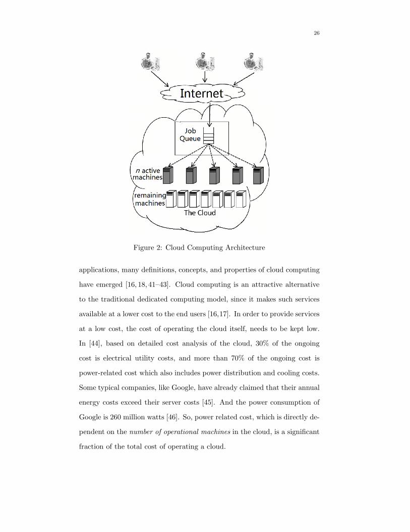
Figure 2: Cloud Computing Architecture
applications, many definitions, concepts, and properties of cloud computing
have emerged [16, 18, 41–43]. Cloud computing is an attractive alternative
to the traditional dedicated computing model, since it makes such services
available at a lower cost to the end users [16,17]. In order to provide services
at a low cost, the cost of operating the cloud itself, needs to be kept low.
In [44], based on detailed cost analysis of the cloud, 30% of the ongoing
cost is electrical utility costs, and more than 70% of the ongoing cost is
power-related cost which also includes power distribution and cooling costs.
Some typical companies, like Google, have already claimed that their annual
energy costs exceed their server costs [45]. And the power consumption of
Google is 260 million watts [46]. So, power related cost, which is directly de-
pendent on the number of operational machines in the cloud, is a significant
fraction of the total cost of operating a cloud.
27
In [43], P. McFedries points out that clouds are typically housed in mas-
sive buildings and may contain thousands of machines. This claim is con-
sistent with the fact that large data centers today often have thousands of
machines [16]. The service system of a cloud can be viewed as a queueing
system. Based on the stability and efficiency discussions in Section 1, we
focus on the behavior of a cloud in the heavy traffic scenarios. Figure 2
shows the basic architecture. Using the new set of heavy traffic limit results
developed in Section 3 and 4, we can achieve the design criteria of power
efficient cloud computing environment, which allows for general and inde-
pendent arrival processes and hyper-exponential distributed service times.
5.1 Heavy Traffic Limits for Different Classes of Clouds
As discussed earlier, it is important that the cloud operates stably, which
means that the traffic intensity ρn should be less than 1. Further, the cloud
also needs to work efficiently, which means that the traffic intensity ρn should
be as close to 1 as possible and should approach 1 as n→ ∞. The different
classes of clouds will result in different heavy traffic limits, and will thus be
governed by different design rules for the number of operational machines
n and traffic intensity ρn. From the known literature [11, 12, 31–33, 47, 48],
one can easily derive the heavy traffic limits for the ZWT and PWT classes.
The derivation is also explicitly shown in our technical report [19], and so,
here, to save space, we simply state how n and ρn should scale to satisfy the
QoS requirements of various clouds.
28
5.1.1 ZWT Class
For a cloud of ZWT Class, using Proposition 1, we observe that
(1 − ρn)√n→ ∞, (71)
from Eqs. (18)-(20). If we define f(n) as 1 − ρn, then
limn→∞
f(n) = 0,
limn→∞
f(n)√n = ∞.
(72)
5.1.2 MWT Class
Applying the result of Proposition 1, we can show that the QoS of a cloud
of MWT Class can be satisfied if
L ≤ limn→∞
(1 − ρn)√n ≤ U. (73)
U and L can be computed from Eq. (6)–Eq. (11) in Proposition 1.
5.1.3 BWT Class
We can satisfy the QoS requirement of this class by applying Proposition 10
to obtain
limn→∞
(1 − ρn)n
− ln δn= τ, (74)
where τ can be computed by Eq. (61) and Eq. (62).
For a cloud of BWT Class, not all functions δn, which decrease to 0, as
n goes to infinity, can satisfy the condition. An appropriate δn that can be
used to satisfy the QoS of BWT Class should satisfy the condition Eq. (60)
given in Proposition 10. Then, the waiting time of jobs for BWT Class is
29
between 0 and t almost surely as n→ ∞.
5.1.4 PWT Class
The QoS requirement of a cloud of PWT Class cloud based on Eq. (64)
satisfies
PWn ≥ t2 ∼ e− 2nµ(1−ρ)t2
µ2σ2+c2 .
For a cloud of PWT Class, to satisfy its QoS requirement, the traffic
intensity must scale as
limn→∞
(1 − ρn)n = γ, (75)
where
γ =−(µ2σ2 + c2) ln δ
2µt2.
Here, µ and σ are same as Eq. (62).
5.2 Number of Operational Machines for Different Classes
As discussed in Section 1, an important motivation of cloud computing is
to maximize the workload that the cloud can support and at the same time
satisfy the QoS requirements of the users. Based on the heavy traffic limits
shown in Sections 3 and 4, we have different heavy traffic limits for different
cloud classes (The details of the ZWT and PWT classes are shown in our
technical report [19]). Thus, in order for the cloud to work efficiently and
economically, we need to compute the least number of machines that the
cloud needs to continue operating for a given QoS requirement.
When ρ is closed to 1 and n is large, the heavy traffic limit is a good
methodology to approximate the relationship between ρ and n. Based on
the heavy traffic limits, we list the minimum number of machines that the
cloud needs to provide under four classes of clouds, as below.
30
• The ZWT class: The ρn and n satisfy that 1 − ρn ∼ f(n). Then, the
number of operational machines n is ⌈f−1(1 − ρ)⌉.
• The MWT class: The ρn and n satisfy that L ≤ (1 − ρn)√n ≤ U .
Then, for the number of optimal machines n, the lower bound is
⌈( L1−ρ )
2⌉, and the upper bound is ⌈( U1−ρ )
2⌉.
• The BWT class: The ρn and n satisfy that (1−ρn)n− ln δn
= τ . Then, the
number of operational machines n is ⌈ τ ln δnρ−1 ⌉.
• The PWT class: The ρn and n satisfy that (1 − ρn)n = γ. Then, the
number of operational machines n is ⌈ γ1−ρ⌉.
Since there are many advanced techniques that can be used to estimate
the parameter ρ and this is not the main focus of this paper, we assume that
the parameter ρ can be estimated from the data. The number of machines
can then be determined by the QoS requirements and the estimated ρ, as
shown above.
6 Numerical Analysis
6.1 Evaluation Setup
We assume that the cloud can accommodate at mostN machines. Clearly, to
reduce power consumption, we want to keep the number of powered servers
to a minimum while at the same time satisfying the corresponding QoS
requirements. The parameters for the four classes are as follows:
1. For the ZWT class, we choose f(n) = n−k1, where k1 = 0.25.
2. For the MWT class, we choose the waiting probability α = 0.005.
31
0.8 0.85 0.9 0.95 10
1000
2000
3000
4000
5000
6000
7000
8000
9000
10000
ρ
n
ZWTMWTBWTPWT
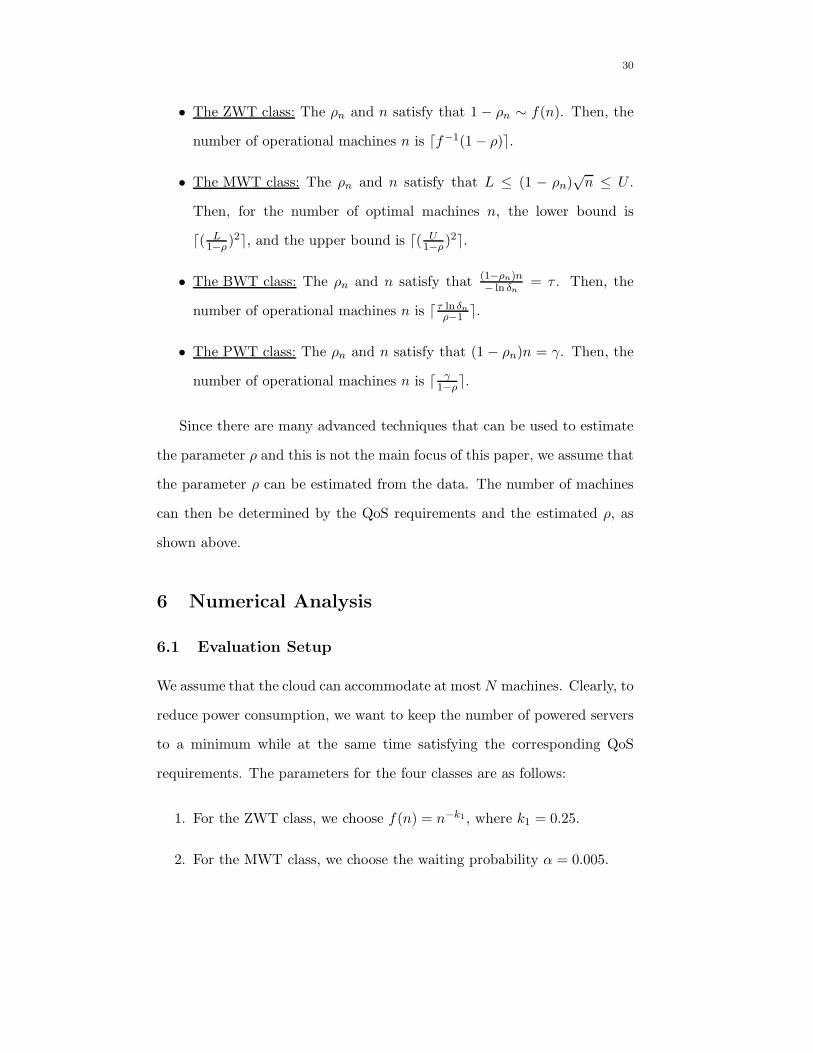
Figure 3: Operational Number of Machines for Exponential DistributedService Time
3. For the BWT class, we choose δn = exp (−n 14 ), which satisfies Eq.
(60), and t1 = 0.5.
4. For the PWT class, we choose the probability threshold δ = 0.1 and
t2 = 1.
6.2 Necessity of Class-based Design
We first choose a simple process–Poisson process–for arrivals, and choose
an exponential service time distribution (i.e., µ = 0.3, which is the simplest
case of the hyper-exponential distribution).
The results characterizing the relationship between the number n of re-
quested machines and the traffic intensity ρ are shown in Fig. 3 for N =
10000. The figure shows that with a larger pool of machines, not only a
large number of jobs, but also a higher intensity of the offered load can be
sustained, especially for clouds with more stringent QoS requirements.
From Fig. 3, we can also see that the number of machines needed for
a given value of ρ is quite different for different QoS classes. Classes with
32
0.75 0.8 0.85 0.9 0.95 10
1000
2000
3000
4000
5000
6000
7000
8000
9000
10000
ρ
n
ZWTMWT (Upper Bound)MWT (Lower Bound)BWTPWT
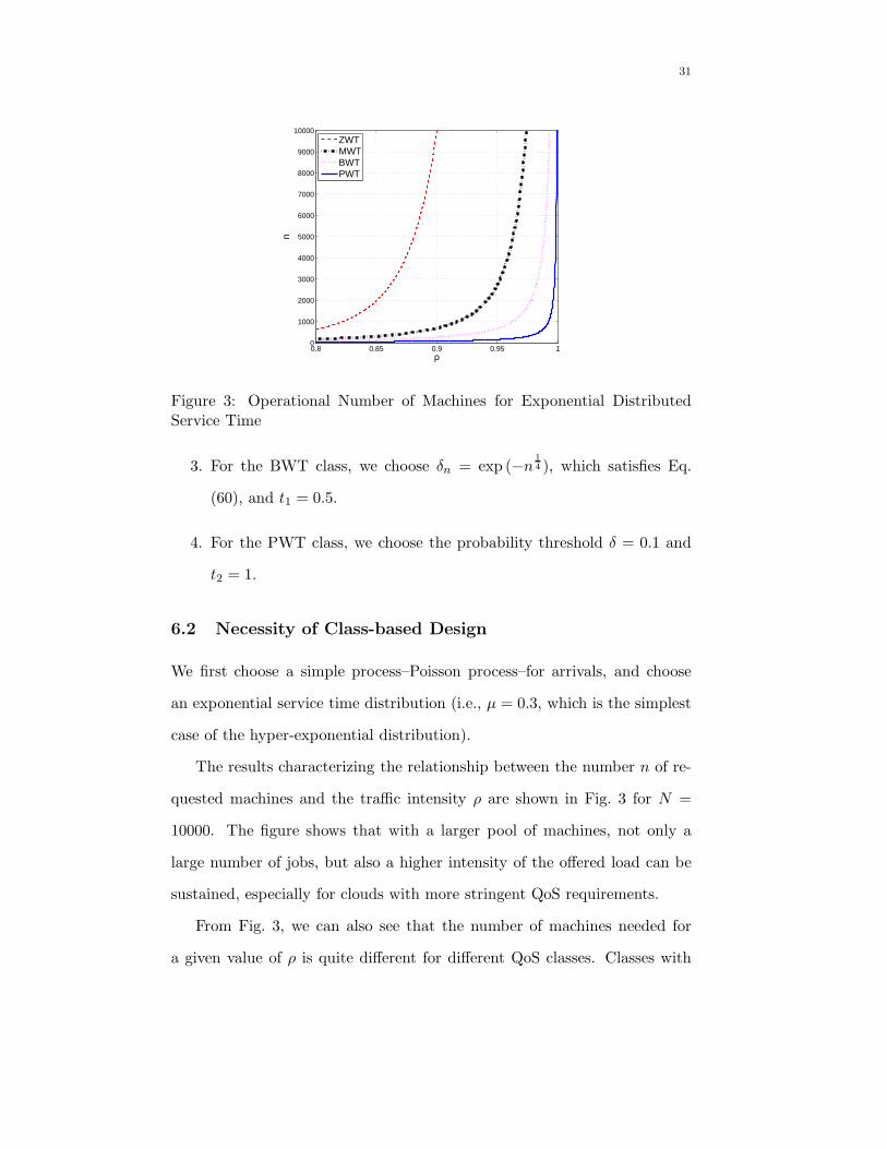
Figure 4: Operational Number of Machines for Hyper-exponential Dis-tributed Service Time
higher QoS require several times more machines than classes with lower QoS
under the same traffic intensity ρ, which implies that different number of
operational machines are necessary for different QoS classes, even for the
simplest case in our scenarios.
In Fig. 4, we now choose a hyper-exponential distributed service time,
with µ = [1 8 20] and P = [0.6 0.25 0.15]. The results characterizing the
relationship between the number n of requested machines and the traffic
intensity ρ are shown in Fig. 4 for N = 10000. The figure is similar to the
exponential distributed service time case shown in Fig. 3. The difference
is that there are only upper and lower bounds for the MWT class in this
scenario. However, even though there is a certain gap between the upper
and lower bounds for the MWT class, the number of requested operational
machines is still different from other classes when n is large enough.
Note that Figs. 3 and 4 can also be used to find the maximal traffic
intensity a cloud can support while satisfying a given QoS requirement for
a given number of machines in the cloud.
33
0 2000 4000 6000 8000 1000010
0
101
102
103
104
λ
Add
ition
al N
umbe
r of
Mac
hine
s
ZWTMWTBWTPWT
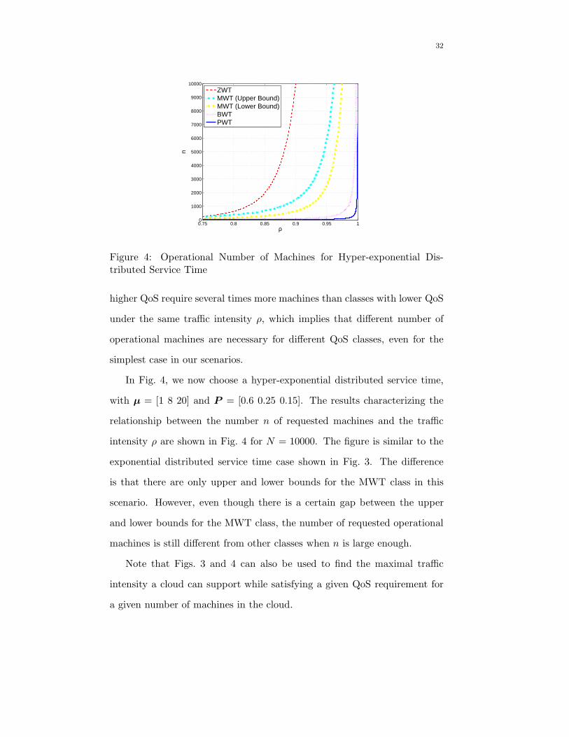
Figure 5: Additional Operational Machines for Exponential Distributed Ser-vice Time
0 2000 4000 6000 8000 1000010
0
101
102
103
104
λ
Add
itona
l Num
ber
of M
achi
nes
ZWTMWT (Upper Bound)MWT (Lower Bound)BWTPWT
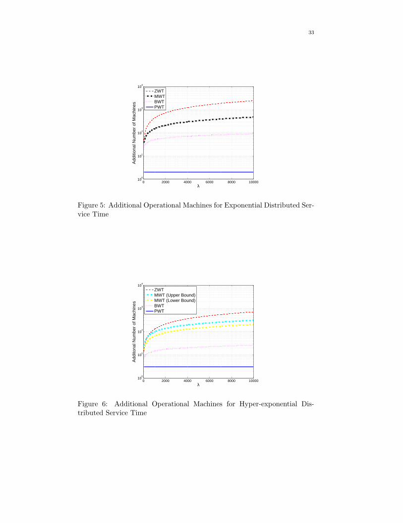
Figure 6: Additional Operational Machines for Hyper-exponential Dis-tributed Service Time
34
0 2000 4000 6000 8000 100000.4
0.5
0.6
0.7
0.8
0.9
1
λ
ρ
ZWTMWTBWTPWT
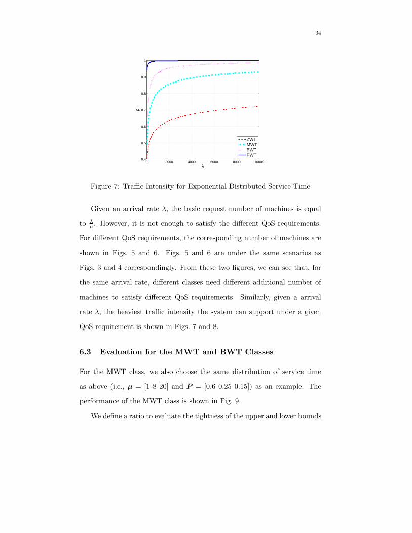
Figure 7: Traffic Intensity for Exponential Distributed Service Time
Given an arrival rate λ, the basic request number of machines is equal
to λµ. However, it is not enough to satisfy the different QoS requirements.
For different QoS requirements, the corresponding number of machines are
shown in Figs. 5 and 6. Figs. 5 and 6 are under the same scenarios as
Figs. 3 and 4 correspondingly. From these two figures, we can see that, for
the same arrival rate, different classes need different additional number of
machines to satisfy different QoS requirements. Similarly, given a arrival
rate λ, the heaviest traffic intensity the system can support under a given
QoS requirement is shown in Figs. 7 and 8.
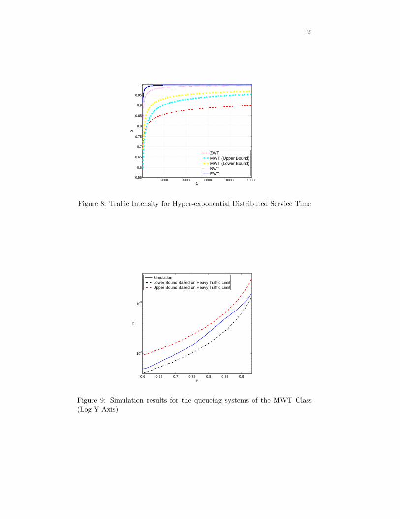
6.3 Evaluation for the MWT and BWT Classes
For the MWT class, we also choose the same distribution of service time
as above (i.e., µ = [1 8 20] and P = [0.6 0.25 0.15]) as an example. The
performance of the MWT class is shown in Fig. 9.
We define a ratio to evaluate the tightness of the upper and lower bounds
35
0 2000 4000 6000 8000 100000.55
0.6
0.65
0.7
0.75
0.8
0.85
0.9
0.95
1
λ
ρ
ZWTMWT (Upper Bound)MWT (Lower Bound)BWTPWT
Figure 8: Traffic Intensity for Hyper-exponential Distributed Service Time
0.6 0.65 0.7 0.75 0.8 0.85 0.9
102
103
ρ
n
SimulationLower Bound Based on Heavy Traffic LimitUpper Bound Based on Heavy Traffic Limit
Figure 9: Simulation results for the queueing systems of the MWT Class(Log Y-Axis)
36
0 0.05 0.1 0.15 0.2 0.25 0.31
1.5
2
2.5
3
3.5
4
4.5
α
r 1
k=1k=2k=5k=20k=100k=1000
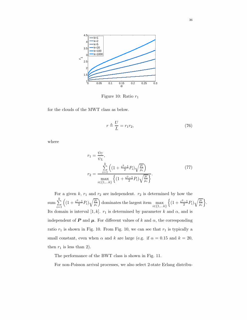
Figure 10: Ratio r1
for the clouds of the MWT class as below.
r ,U
L= r1r2, (76)
where
r1 =ψUψL
,
r2 =
k∑i=1
((1 + c2−1
2 Pi)√
Pi
µi
)
maxi∈1,...k
(1 + c2−1
2 Pi)√
Pi
µi
.(77)
For a given k, r1 and r2 are independent. r2 is determined by how the
sumk∑i=1
((1 + c2−1
2 Pi)√
Pi
µi
)dominates the largest item max
i∈1,...k
(1 + c2−1
2 Pi)√
Pi
µi
.
Its domain is interval [1, k]. r1 is determined by parameter k and α, and is
independent of P and µ. For different values of k and α, the corresponding
ratio r1 is shown in Fig. 10. From Fig. 10, we can see that r1 is typically a
small constant, even when α and k are large (e.g. if α = 0.15 and k = 20,
then r1 is less than 2).
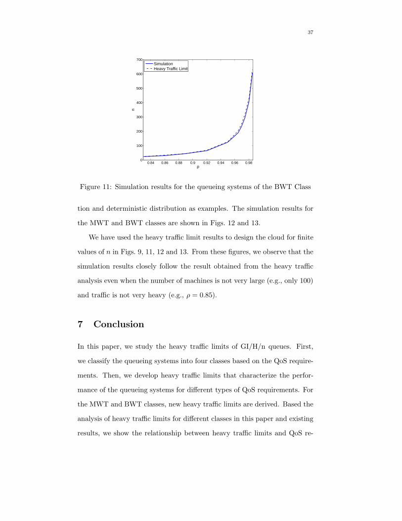
The performance of the BWT class is shown in Fig. 11.
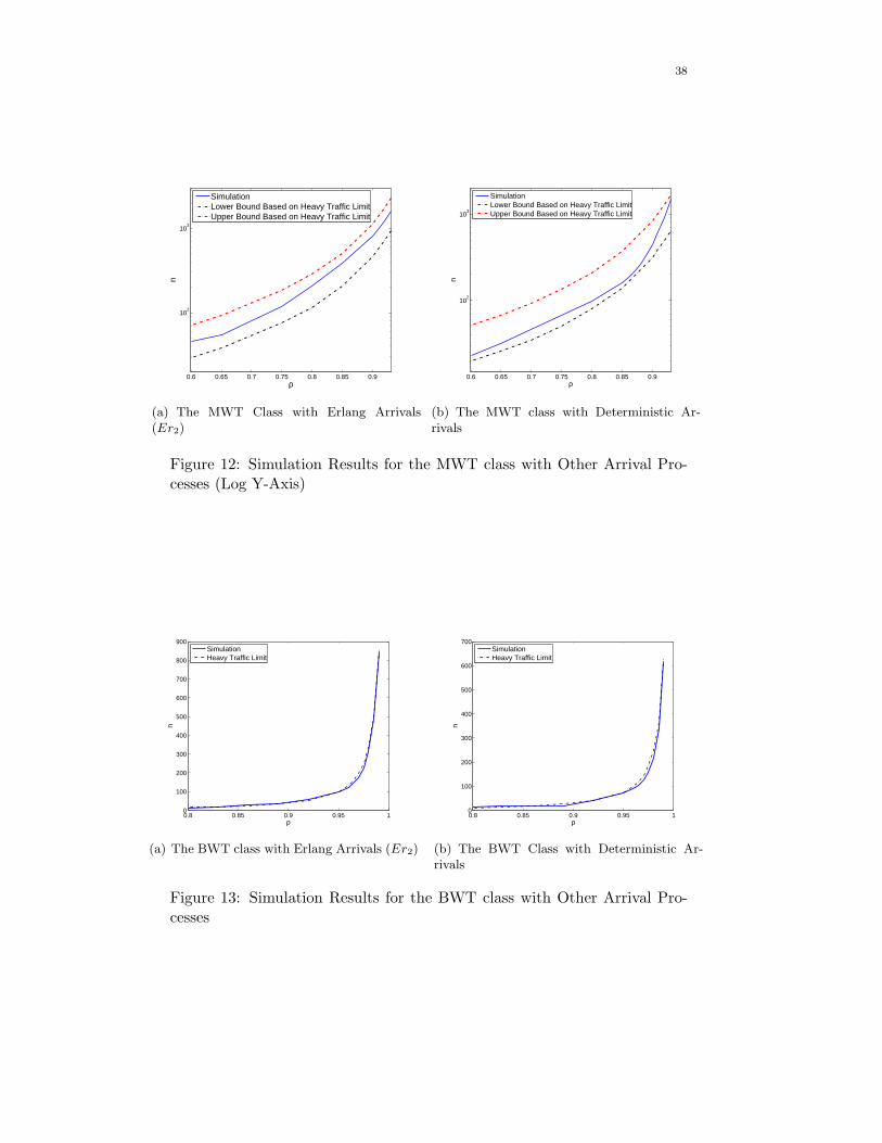
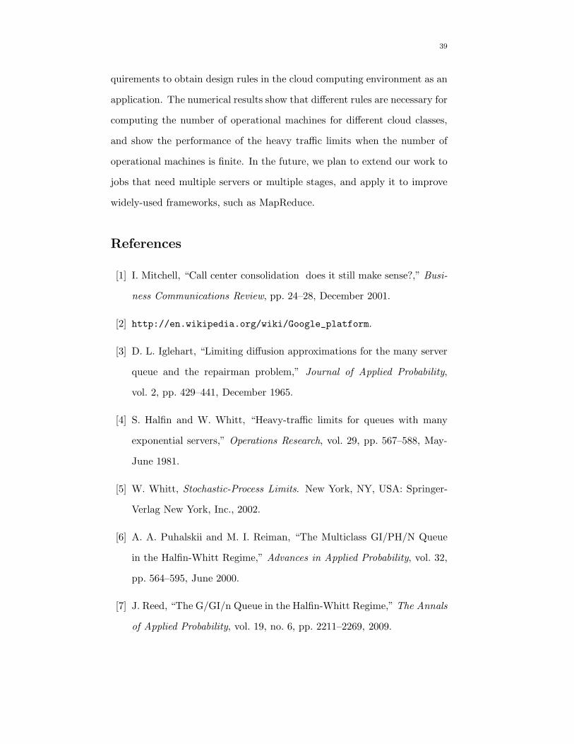
For non-Poisson arrival processes, we also select 2-state Erlang distribu-
37
0.84 0.86 0.88 0.9 0.92 0.94 0.96 0.980
100
200
300
400
500
600
700
ρ
n
SimulationHeavy Traffic Limit
Figure 11: Simulation results for the queueing systems of the BWT Class
tion and deterministic distribution as examples. The simulation results for
the MWT and BWT classes are shown in Figs. 12 and 13.
We have used the heavy traffic limit results to design the cloud for finite
values of n in Figs. 9, 11, 12 and 13. From these figures, we observe that the
simulation results closely follow the result obtained from the heavy traffic
analysis even when the number of machines is not very large (e.g., only 100)
and traffic is not very heavy (e.g., ρ = 0.85).
7 Conclusion
In this paper, we study the heavy traffic limits of GI/H/n queues. First,
we classify the queueing systems into four classes based on the QoS require-
ments. Then, we develop heavy traffic limits that characterize the perfor-
mance of the queueing systems for different types of QoS requirements. For
the MWT and BWT classes, new heavy traffic limits are derived. Based the
analysis of heavy traffic limits for different classes in this paper and existing
results, we show the relationship between heavy traffic limits and QoS re-
38
0.6 0.65 0.7 0.75 0.8 0.85 0.9
102
103
ρ
n
SimulationLower Bound Based on Heavy Traffic LimitUpper Bound Based on Heavy Traffic Limit
(a) The MWT Class with Erlang Arrivals(Er2)
0.6 0.65 0.7 0.75 0.8 0.85 0.9
102
103
ρ
n
SimulationLower Bound Based on Heavy Traffic LimitUpper Bound Based on Heavy Traffic Limit
(b) The MWT class with Deterministic Ar-rivals
Figure 12: Simulation Results for the MWT class with Other Arrival Pro-cesses (Log Y-Axis)
0.8 0.85 0.9 0.95 10
100
200
300
400
500
600
700
800
900
ρ
n
SimulationHeavy Traffic Limit
(a) The BWT class with Erlang Arrivals (Er2)
0.8 0.85 0.9 0.95 10
100
200
300
400
500
600
700
ρ
n
SimulationHeavy Traffic Limit
(b) The BWT Class with Deterministic Ar-rivals
Figure 13: Simulation Results for the BWT class with Other Arrival Pro-cesses
39
quirements to obtain design rules in the cloud computing environment as an
application. The numerical results show that different rules are necessary for
computing the number of operational machines for different cloud classes,
and show the performance of the heavy traffic limits when the number of
operational machines is finite. In the future, we plan to extend our work to
jobs that need multiple servers or multiple stages, and apply it to improve
widely-used frameworks, such as MapReduce.
References
[1] I. Mitchell, “Call center consolidation does it still make sense?,” Busi-
ness Communications Review, pp. 24–28, December 2001.
[2] http://en.wikipedia.org/wiki/Google_platform.
[3] D. L. Iglehart, “Limiting diffusion approximations for the many server
queue and the repairman problem,” Journal of Applied Probability,
vol. 2, pp. 429–441, December 1965.
[4] S. Halfin and W. Whitt, “Heavy-traffic limits for queues with many
exponential servers,” Operations Research, vol. 29, pp. 567–588, May-
June 1981.
[5] W. Whitt, Stochastic-Process Limits. New York, NY, USA: Springer-
Verlag New York, Inc., 2002.
[6] A. A. Puhalskii and M. I. Reiman, “The Multiclass GI/PH/N Queue
in the Halfin-Whitt Regime,” Advances in Applied Probability, vol. 32,
pp. 564–595, June 2000.
[7] J. Reed, “The G/GI/n Queue in the Halfin-Whitt Regime,” The Annals
of Applied Probability, vol. 19, no. 6, pp. 2211–2269, 2009.
40
[8] D. Gamarnik and P. Momcilovic, “Steady-state analysis of a multi-
server queue in the Halfin-Whitt regime,” Advances in Applied Proba-
bility, vol. 40, no. 2, pp. 548–577, 2008.
[9] W. Whitt, “Heavy-Traffic Limits for the G/H∗2/n/m Queue,” Mathe-
matics of Operations Research, vol. 30, pp. 1–27, February 2005.
[10] W. Whitt, “A Diffusion Approximation for the G/GI/n/m Queue,”
Operations Research, vol. 52, pp. 922–941, November-December 2004.
[11] O. Garnett, A. Mandelbaum, and M. I. Reiman, “Designing a call cen-
ter with impatient customers,” Manufacturing & Service Operations
Management, vol. 4, pp. 208–227, Summer 2002.
[12] S. Borst, A. Mandelbaum, and M. I. Reiman, “Dimensioning large call
centers,” Operations Research, vol. 52, pp. 17–34, Janurary-February
2004.
[13] A. Bassamboo, J. M. Harrison, and A. Zeevi, “Design and Control of
a Large Call Center: Asymptotic Analysis of an LP-based Method,”
Operations Research, vol. 54, pp. 419–435, May-June 2006.
[14] M. Armony, I. Gurvich, and A. Mandelbaum, “Service Level Differenti-
ation in Call Centers with Fully Flexible Servers,” Management Science,
vol. 54, pp. 279–294, February 2008.
[15] N. Gans, G. Koole, and A. Mandelbaum, “Telephone Call Centers:
Tutorial, Review, and Research Prospects,” Manufacturing & Service
Operations Management, vol. 5, no. 2, pp. 79–141, 2003.
[16] M. Armbrust, A. Fox, R. Griffith, A. Joseph, R. Katz, A. Konwinski,
G. Lee, D. Patterson, A. Rabkin, I. Stoica, and M. Zaharia, “Above the
41
clouds: A berkeley view of cloud computing,” tech. rep., UC Berkeley,
February 2009.
[17] R. Buyya, C. S. Yeo, and S. Venugopal, “Market-oriented cloud com-
puting: Vision, hype, and reality for delivering it services as computing
utilities,” in Proceedings of High Performance Computing and Commu-
nications, 2008. HPCC’08, pp. 5–13, September 2008.
[18] L. M. Vaquero, L. Rodero-Merino, J. Caceres, and M. Lindner, “A
break in the clouds: Towards a cloud definition,” AMC SIGCOMM
Computer Communication Review, vol. 39, pp. 50–55, January 2009.
[19] Y. Zheng, N. Shroff, P. Sinha, and J. Tan, “Design of a power efficient
cloud computing environment: heavy traffic limits and QoS,” tech. rep.,
Ohio State University, February 2011.
[20] M. Lin, A. Wierman, L. Andrew, and E. Thereska, “Jayakrishnan nair
and adam wierman and bert zwart,” in 48th Annual Allerton Confer-
ence on Communication, Control, and Computing, 2010. Allerton’10,
pp. 969–976, Feburary 2010.
[21] A. Wierman and B. Zwart, “Is tail-optimal scheduling possible?.”
[22] A. L. Stolyar, “Control of end-to-end delay tails in a multiclass net-
work: Lwdf discipline optimality,” Business Communications Review,
pp. 1151–1206, 2003.
[23] A. L. Stolyar and K. Ramanan, “Largest weighted delay first scheduling:
large deviations and optimality,” The Annals of Applied Probability,
vol. 11, no. 1, pp. 1–48, 2001.
[24] J. F. C. Kingman, Poisson Processes. New York, NY, USA: Oxford
University Press, USA, 1993.
42
[25] D. J. Daley, “Certain optimality properties of the first come first served
discipline for g/g/s queues,” Stochastic Processes and their Applica-
tions, vol. 25, pp. 301–308, 1987.
[26] W. Whitt, “The amount of overtakingin a network of queues,” Stochas-
tic Processes and their Applications, vol. 14, pp. 411–426, 1984.
[27] Z. Liu and D. Towsley, “Stochastic scheduling in in-forest networks,”
Advances of Applied Probability, vol. 26, pp. 222–241, 1994.
[28] S. G. Foss and N. I. Chernova, “On optimality of the fcfs discipline
in multiserver queueing systems and networks,” Siberian Mathematical
Journal, vol. 42, pp. 372–385, March-April 2001.
[29] S. Ross, Stochastic Processes. New York, NY, USA: John Wiley & Sons,
1996.
[30] P. BIllingsley, Probability and Measure. New York, NY, USA: John
Wiley & Sons, 1995.
[31] J. F. C. Kingman, “The heavy traffic approximation in the theory of
queues,” in Proceedings of Symposium on Congestion Theory, pp. 137–
159, 1965.
[32] J. Kollerstrom, “Heavy Traffic Theory for Queues with Several Servers.
I,” Journal of Applied Probability, vol. 11, pp. 544–552, September 1974.
[33] J. Kollerstrom, “Heavy Traffic Theory for Queues with Several Servers.
II,” Journal of Applied Probability, vol. 16, pp. 393–401, June 1979.
[34] J. McCarthy, “Mit centennial,” 1961.
43
[35] J. Broberg, S. Venugopal, and R. Buyya, “Market-oriented grids and
utility computing: The state-of-the-art and future directions,” Journal
of Grid Computing, vol. 6, pp. 255–276, September 2008.
[36] P. Sharma, “Core characteristics of web 2.0 services.” http://www.
techpluto.com/web-20-services/, November 2008.
[37] http://code.google.com/appengine.
[38] http://aws.amazon.com/ec2.
[39] http://aws.amazon.com/s3.
[40] http://www.microsoft.com/windowsazure/.
[41] J. Geelan, “Twenty one experts define cloud computing,” Virtualiza-
tion, Electronic Magazine, August 2008.
[42] R. Bragg, “Cloud computing: When computers really rule,” Tech News
World, Electronic Magazine, July 2008.
[43] P. McFedries, “The cloud is the computer,” IEEE Spectrum Online,
Electronic Magazine, August 2008.
[44] A. Greenberg, J. Hamilton, D. A. Maltz, and P. Patel, “The cost of a
cloud: research problems in data center networks,” ACM SIGCOMM
Computer Communication Review, vol. 39, pp. 68–73, Janurary 2009.
[45] http://greenit.net/whygreenit.html.
[46] J. Glanz, “Google details, and defends, its use of elec-
tricity.” http://www.nytimes.com/2011/09/09/technology/
google-details-and-defends-its-use-of-electricity.html,
September 2011.
44
[47] L. Kleinrock, Queueing Systems, Volumn 1: Theory. New York, NY,
USA: John Wiley & Sons, 1975.
[48] L. Kleinrock, Queueing Systems, Volumn 2: Computer Applications.
New York, NY, USA: John Wiley & Sons, 1976.
Related Documents


