Heavy traffic analysis of a transportation network model

HD28.M414

I* DEWEY

WORKING PAPER

ALFRED P. SLOAN SCHOOL OF MANAGEMENT

Heavy Traffic Analysis of a

Transportation Network Model

William P. Peterson

Lawrence M. Wein

#3673-94-MSA April 1994

MASSACHUSETTS

INSTITUTE OF TECHNOLOGY50 MEMORIAL DRIVE

CAMBRIDGE, MASSACHUSETTS 02139

Heavy Traffic Analysis of a

Transportation Network Model

William P. Peterson

Lawrence M. Wein

#3673-94-MSA April 1994

JM.I.T. LIBRARfES^

I MAY 1 ? 1994

I RECEIVED

HEAVY TRAFFIC ANALYSIS OF ATRANSPORTATION NETWORK MODEL

William P. Peterson ^

Operations Research Center. M.I.T.

and

Lawrence M. Wein ^

Sloan School of Management, M.I.T.

Abstract

We study a model of a stochastic transportation system introduced by Crane. By

adapting constructions of multidimensional reflected Brownian motion (RBM) that have

since been developed for feedforward queueing networks, we generalize Crane's original func-

tional central limit theorem results to a full \ector setting, giving an explicit development for

the case in which all terminals in the model experience heavy traffic conditions. We investi-

gate product form conditions for the stationary distribution of our resulting RBM limit, and

contrast our results for transportation networks with those for traditional queueing network

models.

Keywords. Transportation networks, queueing, heavy traffic, reflected Brownian motion.

AMS 1991 subject classification. Primary: 90B22, 60K25. Secondary: 60F17.

April 11, 1994

'Resecirch supported by Middlebury College under the Faculty Leave Program.

^Reseajch supported by National Science Foundation grant DDM-9057297.

1 Introduction and Summary

In this paper, we prove a heavy traffic limit theorem for a transportation system model

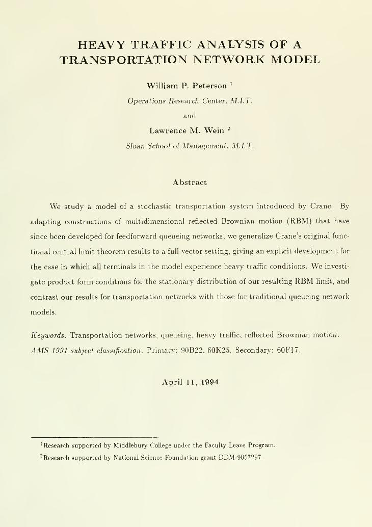
introduced by Crane (1974). The model, depicted in Figure 1, is given a full mathematical

formulation in Section 2. To summarize, the system under consideration consists of a linear

network of A'^ + 1 terminals, indexed i = 0. 1, .... ^V. The network is served by a fleet of

M vehicles, each having fixed passenger capacity V. The fleet is partitioned into service

groups ^i, . ..

, 5/v- Vehicles in group S, are initially dispatched from terminal and proceed

directly to terminal z, where they pick up waiting passengers. They make successive stops

at i — 1, . ..

, 1 to discharge and pick up passengers, then I'eturn to terminal 0, where all

remaining passengers disembark. This cyclic route is repeated indefinitely by each vehicle

in the group. Terminals i = 1 N each have an exogenous arrival stream of prospective

passengers. Passengers arriving to terminal i require transportation to one of the terminals

t — 1, ... ,0. They join a single queue at i. and board arriving vehicles in a first-come first-

served (FCFS) fashion subject to availability of seats. There is no bound on the number of

passengers that can be queued at any station, and it is assumed that prospective passengers

do not balk or renege. As Crane notes, this model can be applied to a public transportation

system, such as a municipal subway line, in which there are no pubhshed schedules and

passengers arrive without reservations. His paper appears to be the only previous attempt

to analyze the performance of a dynamic stochastic network model of a pubhc transportation

system with limited vehicle capacity.

Crane presents functional central limit theorem results for his model, of the type ob-

tained in the seminal papers of Iglehart and Whitt (1970) on queueing systems. Because

the theory of what is now called multidimensional reflected Brownian motion was unknown

at the time, Crane was able to explicitly describe his limit processes only for the case in

which a single terminal in the network is critically loaded, in the sense that the exogenous

passenger arrival rate at the terminal equals the rate at which vehicle capacity is provided

there. Even in that case, the covariance manipulations presented are quite cumbersome. Our

1 Group

multiclciss queueing networks described in Harrison and Nguyen (1993). In particular, in the

form of the reflection matrix one can identity both customer routing effects (i.e., passenger

destination information) and vehicle effects: the queueing models cited include only the

former. We discuss this in the context of an example in Section 5. On a negative note, it

will be seen there that except in artificial special cases, the RBM limit can never satisfy the

conditions for a product form stationary distribution. We show in terms of the covariance

structure of the RBM why this is the case. However, it should be noted that even though

the stationary distribution cannot be found analytically, the numerical methods recently

developed by Dai and Harrison (1992) for steady-state analysis of RBM on an orthant can

be applied to analyze system performance in our model.

Our limit results are formulated in terms of weak convergence in product spaces D'^ for

appropriate dimension d, where D = D[0,T] is the space of real-valued functions on [0,7"]

that are right continuous and have left hand limits, under the Skorohod topology. Weak

convergence will be denoted by ^. .A.11 vectors are to be understood as column vectors, with

primes used to indicate matrix and vector transpose.

2 The Model

We begin by summarizing the probabiHstic structure of the model, following the treatment

in Crane. Three basic phenomena need to be described: exogenous passenger arrivals to

the system, passengers' choice of destination terminals, and circulation of vehicles in the

network. For simplicity, it is assumed that there are no passengers in the network at time

t = 0, and that all of the vehicles in the fleet begin their routes from terminal i — at that

time. For present purposes, these assumptions have no significant effect on our limit results.

For i = 1,...,A'^, set u,(0) = and for / = 1,2,... let the random variable ii,(/)

represent the /"* interarrival time in the exogenous passenger arrival stream to terminal (.

Define the counting processes

A,{i) = max{/>0:u,(0) + u,(l) + - •• + «,(/) < ^} (1)

3

for t > 0, so that .4,(<) represents the number of exogenous passenger arrivals to terminal ;'

over [0, i].

Passenger destination selection is described by an A'^ x N matrix F = (7,^). We as-

sume that a passenger arriving to terminal /' has destination terminal j with probabihty

7,_,, independent of the destination of any other passenger. As described in the last section,

passengers always seek transportation to lower numbered terminals, so 7,^ = for j > i\

in other words, T is strictly lower triangular. .Also, 1 — Z]j=i 7u '^ ^^e probability that a

passenger originating at i has destination terminal 0. We introduce for each terminal i a

sequence of i.i.d. A'^-dimensional random vectors \,(/) = (.\i,i(Oi • • 1 \t.iv(0)'- where x,j{l)

is equal to 1 if the /"* passenger in the arrival stream to i has destination j, and is zero

otherwise. Observe that £'[\,(1)] = F^, where F, denotes the i*'' row of F. Next define the

A'^- dimensional cumulative sum processes U, = {Ui{r),r — 1,2, . . .} by

ihir) = \Al) + --- + \.(r). (2)

Then the j"* component of U,{r), which we shall denote by U,j(r), gives the number of

passengers among the first r arrivals to terminal i who have destination j.

Recall that vehicles k = 1, ..., M have been partitioned into service groups 5,. Consider

a vehicle k G 5,. We introduce sequences of random variables {t'fc,j(/). / = 1,2,...} for

j = 0, 1, . ..

, z, where Vk,j{l) represents the transit time for the vehicle's /"* trip along the link

starting from terminal j; this hnk goes to terminal j — I if j > 1, and to terminal ; if j = 0.

It is assumed that when a vehicle arrives at a station, any passengers it is carrying who

are destined for that station disembark instantaneously, and any waiting passengers then

instantaneously board subject to availabilit\- of space. With this understanding, we define

u^fc(l) = i.'«:,o(l). and

io,{l) = vUn + i2''^-J^-^)^ / = 2,3,... .

Then the sequence {wk{l), I = 1,2,...} gi\es the times between successive visits of the

vehicle to terminal i. Define the corresponding counting processes {C\-(t), t > 0} by

^ . . / max{/:a',(l) + --- + u',(/) <0, iiwk{l)<t,

[ 0, if wt,{l) > t.

Now recalhng that each vehicle has fixed capacity V, we see that for / = 1, . ..

, A^,

G,{t) = \-J2C,(t) (4)

kes,

gives the total number of units of vehicle capacity (i.e., available passenger spaces on vehicles)

provided at terminal i during [0,^] by vehicles in service group S,.

Two comments are in order here pertaining to the circulation of vehicles. First, as

noted by Crane, the above framework can be used to accommodate a stochastic idle time

at the terminals, by simply envisioning that such a delay has been incorporated in the most

recent link transit time. Observe, however, that this does not allow the idle time to depend

in any way on passenger data. Second, the model fails to capture any interaction between

the travel times for different vehicles. This would become an issue if passing of vehicles were

not permitted, as would be the case with a single track rail system, for example. In his

dissertation. Crane (1971) outhnes an approach to incorporating such dependencies into the

model.

The counting processes {Ai(<), t > 0} and {G',(i). t > 0}, and the vector sum processes

{U,{r), r = 1,2,...} for j = 1, . ..

, A'^, are assumed to be mutually independent. These are

the basic building blocks for our system representation. We proceed somewhat differently

from Crane, developing a streamlined description that facihtates the proof of our vector

limit theorem. Let Z,(i) denote the number of passengers waiting at terminal ;' at time

t, Ei{t) denote the number of passengers who have boarded vehicles at terminal i during

[0,<], and Yi{t) denote the cumulative number of units of capacity that go unoccupied on

vehicles departing from station i during [0./]. The following is a recursive construction of

representations for these processes. Let

AV(i)-.4v(^)-GV(0^ and (5)

.V

'=.1+1

-Y]+,it] + <,(t), j = N-L...,U (6)

where, ior j = N, . . . ,1,

YAt) = - mf {A-,(.)}, (7)0<s<i

Z,{t) = XAn + Yjit) and (8)

E^t) = AAt)-Z,{t). (9)

The idea here is to construct Xj as a netput process; that is, Xj{t) represents the difference

between the total number of passengers arriving to station j during [0. t] and the cumulative

number of units of vehicle capacity provided there over that time period. If one accepts this

interpretation of (5)-(6), then (7) and (S) are standard representations from the queueing

literature, and (9) is simple bookkeeping. To understand (5)-(6), observe that there are

effectively three ways that vehicle capacity can be provided at ;'. The first is through arrival

of vehicles in service class 5j, as accounted for in the basic process Gj. This is the only

source of capacity at terminal j = -'V, so A'.v can be defined in (5) entirely in terms of basic

processes; this gets the recursion started. .\t terminals j < N, there are two additional

sources of capacity represented in (6). .\rri\ing vehicles from service classes 5, for i > j

provide capacity at j when they are carrying passengers whose destination is j, since these

passengers immediately disembark there, which frees up space for passengers queued at j.

Note that U,j{E,{t)) gives the number of passengers with destination j among the E,(t)

who board vehicles at i during [0,^]. In addition, unused capacity on vehicles departing

from terminal j + 1 during [0,i], as represented by Yj+i{t), will provide capacity when those

vehicles reach j. The £_,(<) is an error term, which is required because the vehicles whose

available capacity is accounted for by U,j(E,{f)) and Yj+i(t) may not have reached terminal

j by time t. Observe, however, that a vehicle can contribute to ej(t) only if that vehicle is

in transit somewhere between terminals i and j for some / > j at time t. Thus, at any time.

the error is certainly bounded by the total capacity of the fleet:

0<tj(t)<MV for all f > 0. j = l iV - 1. (10)

Using this bound, the error will be shown to be negligible under the heavy traffic reseating

to be defined in the next section.

We conclude this section with representations for the queue length and departure

processes at the terminals broken out by passenger destination. At each terminal z, let

Q,j{t) be the number of customers waiting at terminal i whose destination is terminal j,

for j = 0, . . . ,i — I. Similarly let D,j{t) be the number of passengers who have departed

from i whose destination is j. Then for z = i .V we have the following straightforward

representations:

Q„[t) = U,j{Mt)) - U,j{E,it))- j = h...,i-l, (11)

Q,o{t) = Z.(i)-EQu(0, (12)

D,j{t) = U,,[EM)). 7 = L....z-l, and (13)

D.o(0 = EM)-'Y.D.,{t)- (14)

The compound processes Z),j were already introduced, though not explicitly named, in dis-

cussing equation (6). Separating them out in this way will be convenient for developing the

main theorem. The processes (J.j will be treated in a corollary to that theorem, where it will

be shown that their limit processes are given by deterministic fractions of the limit for the

total queue length Z, at each terminal i. This is a manifestation of the state space collapse

phenomenon in heavy traffic results.

3 The Heavy Traffic Conditions

The precise statement of our results involves a sequence of systems, of the type described in

Section 2, approaching conditions of perfect balance between passenger arrivals and vehicle

capacity at each terminal. Hereafter, a superscript n will be used to index processes and

parameters associated with the n"' system in the sequence. We will allow the passenger

interarrival and vehicle transit time distribui ions to vary, so that the basic processes .4" =

(Ai,...,A^) and G" = (G'j, . . . ,6'JV) depend on n. For simplicity, however, we assume

that the destination probabihty matrix T is fixed, which implies that the vector processes

Ui = {Uii, . . . , U,n) for z = 1, . . . , A' do not vary with n.

We require that there exist sequences of .V-dimensional vectors {A"} and {/i"} so that

the scaled processes A" and G" defined by

A"(0 = n-'^-iA^int)- X^nt) (15)

G"(i) = n-'^-(G^{nt) - S'^nt) (16)

satisfy functional central limit theorems (f.c.l.t.'s). For example, if the component arrival

processes A" and the round trip counting processes C^ underlying the G" in (4) are mutually

independent renewal processes, then the required results can be established under some

additional moment assumptions. By (2), f ,(/) has a multinomial distribution for each r, so

the classical Donsker theorem gives f.c.l.t.'s for the processes C^" defined by

0:^(1) = n-'^HU,{[nt\)-T\nt), t = l,...,N. (17)

Therefore, recalHng the assumed independence of A", G" and the U,'s, we have

(i", G", 6T, . .. , UJ^,) ^ [A', G', Ul ...,Un) (18)

as n —»• oo, where the processes on the right aie .V + 2 independent, zero drift, jV-dimensional

vector Brownian motions, whose covariancc matrices will be denoted by 11,4, Sg and S^,

,

i = h...,N.

The definitions in (15)-(17) consist of a centering of key processes followed by the

heavy traffic rescaling, in which time is scaled by n and space by n~^^^. The convergence

in (18) gives the following interpretation of the centering parameters: A" is the long run

average arrival rate to station z, and /3" is the long run average rate at which units of vehicle

capacity are provided by vehicles in 5,. Ignoring the rescahng for the moment, we introduce

the following centered versions of our basic processes. Define:

G'"(f) = G'^lO-^i"^ and (19)

Udt) = L;{[t\)-r',t.

We can later construct the tilde processes in (15)-(17) from these by rescahng; for example,

A'^(t) = n~^/^A"(n/). For now, as an intermediate step, we seek to rewrite the system

state equations from Section 2 in terms of the centered processes. Anticipating the balanced

loading conditions, we expect the long run departure rates to match the corresponding arrival

rates, so the following defines a natural centering for the departure processes:

£"(i) = £"(0 -A"^ (20)

Recall from (13) that Df^(t) = U,j{E^(t)), and observe that

u.AE^it)) = r.,(£r(^)) + 7.,^r(o

This suggests the centering

D:^{t) = U,,{E^{t))-X:f,,t, (21)

where A"7,j can be interpreted as the long run rate at which customers destined for termi-

nal j board vehicles at terminal ;'. By solving (19)-(21) for the uncentered processes and

substituting into (5)-(9), our system state equations become

X;^(i) = A''^{t)-Cr^{t) + {\l--3lr)t, and (22)

-y;;i(0 + e;(0- j = .v-i,....i, (23)

where, for j = 1 , . ..

, A'^

^i"(^) = -o^'JL^-^'"^^)^(-^'

Z;(0 = Xj{f) + y;{t) and (25)

E^it) = .4;(f)-z;(o. (26)

Consideration of the rescaling to follow leads to our heavy traffic conditions. We suppose

that as n —> oo,

A" ^ A > and ^" ^ /3 > (27)

in such a way that, for j = 1, . ..

, A'^,

V^(\" - ^r - E K'lu) - Oj, -^<0,< ^. (28)

This requires that the quantity in parentheses in (28) converge to zero; it also specifies a

common rate of convergence for all terminals j. Following our earlier discussion, A".7,j can

also be interpreted as the long run rate at which customers who originated at i disembark at

terminal j. Therefore, we can see that (27)-(28) describe a sequence of systems approaching

critical loading. In the limit, the exogenous passenger arrival rate to each terminal j is

exactly balanced by the rate at which capacity is provided at j by vehicles in group Sj plus

the rate at which capacity is made available there by passengers disembarking from vehicles

in groups 5, for t > j. Note that by letting 6 = (^j, . . . ,^7v)', we can restate (28) in vector

form as

v^((/-r')A"-,^") ^e. (29)

It is interesting to compare our heavy traffic conditions with the stabihty conditions

derived by Crane. He defines for each terminal an effective service rate fij, which in our

notation would be given for the n"' system by

Here a Ab = min{a,6} and [a]^ = max{a.O}. This set-up explicitly recognizes potential

imbalances in loading. The (A" A^i") acknowledges that the departure rate from terminal / is

bounded by the total rate at which capacity is provided there. The [fi'J+i- ^'}+iV accounts

10

for anv excess vehicle capacity at j + 1. which then becomes axailable capacity at j . Crane's

stability conditions are

A;-//,;<0. for j = l...../V. (31)

We will see that our heavy traffic conditions imply that A" — ^" —> 0. To explore this

relationship completely, write //" = {/.il /.ly]' and define vectors ^" by

r = (/_r')A'' -,i", (32)

Next, introduce an N x N matrix 5 having ones on the main diagonal and negative ones on

the first superdiagonal; that is

[1. if J = i

5., = I -1. if ; = ; + l (33)

I 0. otherwise

Then we have the following.

Proposition 1 The stability conditions (31) hold if and only if

5"^^" <

where the inequality is to be interpreted component-wise.

Proof. First note that S~^ exists and is given by

'"'

I 0. otherwise

If (31) holds, then for each ; we have A; Ai.i'J

= A; and [^; - A;]+ = ^^ - A;. Using this

and (32), we can rewrite (30) as

a;-//; = ^; + (a;^i-/i;^i), ; = a'-i i. (34)

In vector form, this says that 5(A" -^i'') = 0" and the stabihty condition (31) is A" -^z" < 0.

Thus, (31) implies that 5"*^" < 0.

11

Conversely, the scalar form of 5 ^^'^ < is

f:^;<0, . = 1,...,.V. (35)

J='

At i = N, this gives 6"^ < 0. This implies component A^ of (31), because 6^ = AJ^ —

/?J^= A^ — /Zyv by (32) and (30). Suppose inductively that (31) holds for components

j = k + I, . ..

, N . Then, reasoning as above, we see that the equations (34) are valid for

j = k, . ..

, N. Adding these equations gives, after cancellation,

A2-/'i: = E^;- (36)

This imphes A^ - /^^ < by (35).

In the notation just introduced, our hi^avy traffic condition (29) says s/nO"^ — 9. We

will see later that S~^6 < emerges as a necessary condition for positive recurrence of

our RBM limit process. In light of Proposition 1, this means that the process must be

achievable as a limit from a sequence of stable systems. Condition (29) also implies that

9^ —> 0. Following the steps leading to (36) above, this gives A" -/z'' —* in Crane's set-up,

as asserted earher.

4 The Main Theorem

We are now ready to state our main theorem. Define rescaled versions of the vector processes

from our system state description as follows:

X"(0 = n-^I^X^{nt). y'"(0 = ir"^Y"{nt). Z^{t) = n'^/^Z^'int),

Theorem 1 // the the basic functional cailral limit theorems (18) and the heavy traffic

conditions (27)- (28) hold, then

(X".Z". >•'",£") => {X\Z',Y\E').

The limit processes are specified component- ir/.se by

X'^it) = A%.(f)-Gy{t) + 6Mt. and (37)

x;it) = A'^(t)-G;(t)- Y, (f'*(A,0 + 7u^*(0)

+ e^l -l]\,{t), ;=iV-l....,l (38)

where, for j = iV, . ..

, 1,

y'*(-) is continuous and nondecreasing, and (39)

¥'{) increases only when Z'{t) = 0, (40)

Z;{t) = X;(t) + Y;(t) and {U)

E;{t) = A;{t)-z;(t). (42)

Remark 1. The key limit process is Z', the liirdt for the vector queue length process, which

we can characterize as a multidimensional RBM by the following steps. Substituting (38)

into (41) gives

z;{t) = A'(t)-G;[t)- y: {u:^{x^t) + l^JE:it))t=J+l

+ 9,t-Y]\,(n + y;{t). m)

To rewrite this in vector form, introduce the vector process F' defined by

Then F' is a zero drift vector Brownian motion with covariance matrix

Recalling the matrix S defined in (33). we can express (43) as

Z'{t) = A'{t) - G'it) - F-{t) - T'E'it) + et + SY'(t).

Substituting E'(t) = A'{t) — Z'(t). which i-< the vector form of (42), and collecting terms

gives

{I -r)Z'{t) = {I -r)A'{t] -G'{t)-F'{t) + 9t + SY'(t).

13

Because T is strictly upper triangular, (/ — F') is guaranteed to be invertible, so we can solve

the preceding equation for Z'(t). obtaining

Z'it) = A'{t) -(I- r'r'[cr(t) + F'{t)) +rjt + RY-(t), (45)

where

Now setting

T]^{I-r')-'e and R = {I-r')-'S. (46)

at) = A'it) -{I- r')-i [G'it] + F'{t)) + r,t, (47)

equation (45) becomes

Z*{t) =m + RY'it). (48)

Observe that ^ is a vector Brownian motion process with drift vector // and covariance

matrix

Q = S.4 + (/ - r')-\EG + Sf)(/ - T)-\ (49)

Therefore, equation (48), together with the properties (39)-(40) for V'*, identifies Z* as a

multidimensional RBM with drift vector //. covariance matrix Q and reflection matrix R.

Remark 2. The form of the reflection matrix R = (I — r')~^5 has a nice interpretation.

The first factor is attributable to customer effects; the second to vehicle effects. In a tra-

ditional queueing network, only the former would be present. The latter arise here because

unused vehicle capacity at one terminal translates directly into available capacity at the next

terminal downstream. In Section 5 we present a concrete example of these calculations.

Proof of Theorem. Given the recursive representations developed so far, the theorem

can be proved in a straightforward manner by induction, starting at terminal j = .V. By

rescaling equation (22), we obtain the following expression for ,Y^ :

If follows immediately from the basic f.c.l.t.'s for A,\ and Gat, and the heavy traffic condition,

that X;^ =» X*^ = A'^ -G*,^ + ejvc where t{t) = t. This estabhshes (37). Observe that A'^

14

is a one-dimensional Brownian motion process, and therefore continuous. It is easy to check

by rescaling (7)-(9) that

0<s<t

Z^{t) = Xlr{t) + Y^{t) and

E;,{t) = A-yit) - Zl.{t).

By the continuous mapping theorem, we have that {Yjl} , Z^ , E'^) =^ {Yj!^,Z^,E^), jointly

with the result for X^, where

Yi^it) ^ - mUX'^is)},U<s<r

Z'nW = A';v(0 + r^(0 and (50)

£.;.(0 = Ayit)-z'M-

This expresses Yj!^ and Z^ in terms A'^ via the famihar one-dimensional reflection mapping.

Since X]^ is continuous, the first equation here implies properties (39)-(40) for j = N . The

above also verifies (41) and (42) at this terminal.

Now suppose by inductive hypothesis that the results of the theorem hold for terminals

N,N — 1,. . . ,j + I, and consider the situation at terminal j. Rescahng equation (23) gives

X^it) = A]{t)-G]{t)- Yl Dlit)

N

where

-hV^(A;-/?;- Y. ^r7u>->7+i(0 + s"(^)'(si:

A"(<) = n-'l' (U^jiE^int)) - X^f^.nt) . (52)

First note that our basic f.c.l.t.'s give (/i",G'") ^ (AJ,G'J), and by the heavy traffic condition

the deterministic factors multiplying t converge to 9j. For the D" terms, note that £"" => E'

for i = j + I, . ..

, N, by inductive hypothesis. Combining this with the basic result for the

UJj, we can apply the standard Compound Process Functional Central Limit Theorem to

(52) to obtain D^^ =» D'^, where

15

is a Brownian motion process. Also, the inductive hypothesis gives Vj'^j => Vj'+,, where the

limit is continuous. Finally, rescaling (10) gives

< sup P{t) <n-^'^MV0<t<T

for any T > 0. It follows that e" => (, where ({t) = 0. Putting all these terms together in

(51) gives X^ =^ X*, with X^ as in (38). Furthermore, continuity in each term implies that

X' is itself continuous. Now the one-dimensional reflection mapping can be used as in (50)

to get corresponding results for Y' , Zj and E' , thereby establishing (39)-(42).

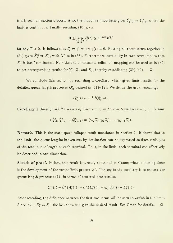
We conclude this section by recording a corollary which gives limit results for the

detailed queue length processes Q"^ defined in (ll)-(r2). We define the usual rescalings

Corollary 1 Jointly with the results of Theorem 1, we have at terminals i = \, . . . , N that

Remark. This is the state space collapse result mentioned in Section 2. It shows that in

the limit, the queue lengths broken out by destination can be expressed as fixed multiples

of the total queue length at each terminal. Thus, in the limit, each terminal can effectively

be described in one dimension.

Sketch of proof. In fact, this result is already contained in Crane; what is missing there

is the development of the vector limit process Z'. The key to the corollary is to express the

queue length processes (11) in terms of centered processes as

Qi(t) = t>(Ar(o) - o^^iE^it)) + 7.;(^r(o - E?it))-

After rescaling, the difference between the first two terms will be seen to vanish in the limit.

Since A" — £^" = Z", the last term will give the desired result. See Crane for details.

16

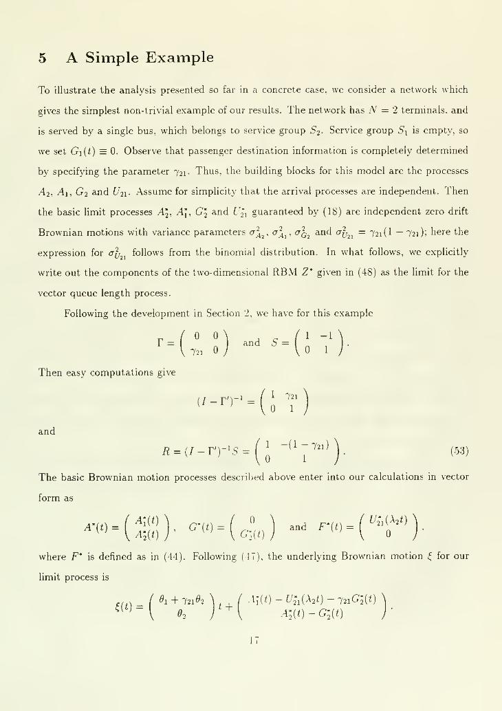
5 A Simple Example

To illustrate the analysis presented so far in a concrete case, we consider a network which

gives the simplest non-trivial example of our results. The network has N = 2 terminals, and

is served by a single bus, which belongs to service group S2- Service group Si is empty, so

we set Gi{t) = 0. Observe that passenger destination information is completely determined

by specifying the parameter 721. Thus, the building blocks for this model are the processes

A2, Ai, G2 and f/2i- Assume for simphcity that the arrival processes are independent. Then

the basic hmit processes Aj, A\, G^ and f',"i guaranteed by (18) are independent zero drift

Brownian motions with variance parameters a\^. a\^ . a^^ and alf^^ = 721(1 — 721); here the

expression for al, follows from the binomial distribution. In what follows, we explicitly

write out the components of the two-dimensional RBM Z' given in (48) as the limit for the

vector queue length process.

Following the development in Section 2, we have for this example

T. / \ , ^ M -i

Then easy computations give

and

:/-r')- = (; '7

^/^-lc / 1 -(1 -721,R = {I-Vr'S= ^ '^

^

"'' 1. (53)

The basic Brownian motion processes described above enter into our calculations in vector

form as

where F' is defined as in (44). Following (47), the underlying Brownian motion ^ for our

limit process is

^^^'[O2 )'^[ A-it)-Gl{t) )

17

1-Y 21

^Figure 2: Directions of reflection for example network.

The drift vector t] is apparent here, and the covariance matrix Q given by (49) is easily

calculated as

On the interior of the nonnegative orthant 5?^, the process Z' = if + RY* behaves like an

(t/, f2) Brownian motion. At the boundary Z' — 0, it is subjected to an "instantaneous

reflection," which corresponds to a displacement in the direction given by the j"* column

of R. This displacement, governed by the increase in Y', is of the minimum magnitude

required to keep the process Z* from leaving the orthant. The direction vectors are shown

in Figure 2.

Hitting the boundary Zj = corresponds to unused capacity on a vehicle departing

terminal 1. This has no effect on the "upstream" terminal 2; hence the direction of reflection

is normal to the boundary. At the other boundary, the situation is more interesting. Hitting

Z2 — corresponds to unused capacity on a vehicle departing terminal 2. This will provide

additional capacity to terminal 1, so we anticipate a negative impact on the queue there.

As noted in Remark 2 following the main theorem, the result is the combination of two

effects, corresponding to the factorization R = {I — r')~^5. The vehicle effect, described by

S, equates unused capacity at terminal 2 unit for unit with available capacity at terminal

18

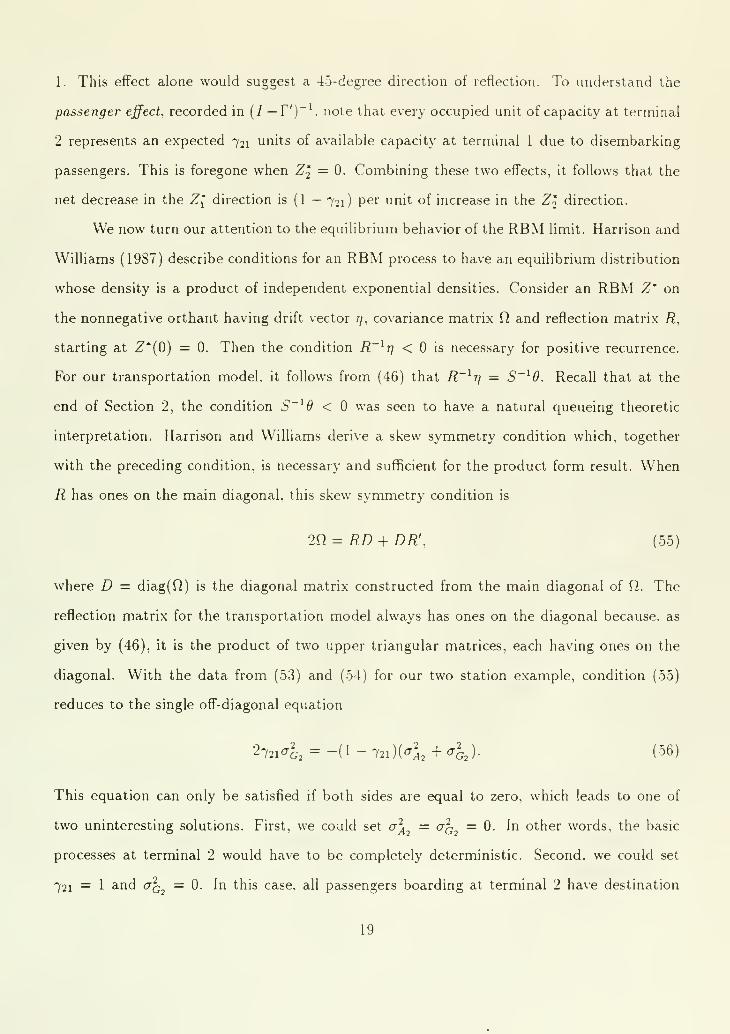
1. This effect alone would suggest a 45-degree direction of reflection. To understand the

passenger effect, recorded in (/ — ^')~^ note that every occupied unit of capacity at terminal

2 represents an expected 721 units of available capacity at terminal 1 due to disembarking

passengers. This is foregone when Z2 = 0. Combining these two effects, it follows that the

net decrease in the Z' direction is (1 — 721) per unit of increase in the Z2 direction.

We now turn our attention to the equihbrium behavior of the RBM limit. Harrison and

Williams (1987) describe conditions for an RBM process to have an equilibrium distribution

whose density is a product of independent exponential densities. Consider an RBM Z' on

the nonnegative orthant having drift vector rj, covariance matrix 17 and reflection matrix R,

starting at Z'{0) = 0. Then the condition R'^r] < is necessary for positive recurrence.

For our transportation model, it follows from (46) that R~^t] = S~^6. Recall that at the

end of Section 2, the condition S~^d < was seen to have a natural queueing theoretic

interpretation. Harrison and Williams derive a skew symmetry condition which, together

with the preceding condition, is necessary and sufficient for the product form result. When

R has ones on the main diagonal, this skew symmetry condition is

2n = RD + DR', (55)

where D = diag(Q) is the diagonal matrix constructed from the main diagonal of U. The

reflection matrix for the transportation model always has ones on the diagonal because, as

given by (46), it is the product of two upper triangular matrices, each having ones on the

diagonal. With the data from (53) and (54) for our two station example, condition (55)

reduces to the single off-diagonal equation

2721 <T^, = -(1 - 721 )(< + O- (06)

This equation can only be satisfied if both sides are equal to zero, which leads to one of

two uninteresting solutions. First, we could set a\^ = a^^ =0. In other words, the basic

processes at terminal 2 would have to be completely deterministic. Second, we could set

721 = 1 and aQ^ = 0. In this case, all passengers boarding at terminal 2 have destination

19

terminal 1, and the vehicle circulation is deterministic. Furthermore, one can see that

analogous problems will be encountered in general for an iV terminal model. The ofF-diagonal

condition relating terminals N and N — 1 will have exactly the form (.56).

Given the lack of interesting solutions to the product form conditions, it is natural to

ask what features of the transportation model make it differ from a conventional queueing

network. The problem arises from the positive covariance between terminals 2 and 1, which

results in the positive left hand side in equation (56). To understand the sign of the co-

variance, note that, away from the boundary, each unit of service by vehicles in group S2

results in 721 units of service capacity for terminal 1. Thus this unit of service effectively

decreases the queue lengths at both terminals, which explains the positive covariance term.

By contrast, in a traditional feedforward queueing network having the same basic topology,

service completions at station 2 would decrease the queue there, but the portion of these

customers routed to station 1 would increase the queue at that station. Hence the corre-

sponding covariance term is negative in this case, and it becomes possible to satisfy the skew

symmetry condition. Solutions for such models are covered by the results of Peterson.

References

Crane, M.A. (1971). Limit theorems for queues in transportation systems. Ph.D. disserta-

tion. Department of Operations Research, Stanford University.

Crane, M.A. (1974). Queues in transportation systems II: an independently dispatched

system. J. Appl. Probab. 11, 145-158.

Dai, J.G. and J.M. Harrison (1992). Reflected Brownian motion in an orthant: numerical

methods for steady-state analysis. Ann. Appl. Probab. 2, 65-86.

Harrison, J.M. (1985). Brownian Motion and Stochastic Flow Systems. New York: .John

Wiley & Sons.

20

Harrison, J.M. and R.J. Williams (1987). .Multidimensional reflected Brownian motions

having exponential stationary distributions. Ann. Probab. 15, 115-137.

Harrison, J.M. and V. Nguyen (1993). Brownian models of multiclass queueing networks:

current status and open problems. Queueing Systems Theory Appl. 13, 5-40.

Iglehart, D.L. and W. Whitt (1970). Multiple channel queues in heavy traffic, 1 and II. Adv.

in Appl. Probab. 2, 150-157 and 355-364.

Peterson, W.P. (1991). A heavy traffic limit theorem for networks of queues with multiple

customer types. Math. Oper. Res. 16, 90-118.

Reiman, M.I. (1984). Open queueing networks in heavy traffic. Math. Oper. Res. 9,

441-458.

21

3878

MIT LIBRARIES

3 TDaO 00843^41 3

r

yiSf/^wr

Date Due

-caa*\jiU.

lf%'%. % "^

Lib-26-67