Heavy-organic particle deposition from petroleum fluid flow in oil

502 DOI 10.1007/s12182-010-0099-4

Heavy-organic particle deposition from petroleum fluid flow in oil wells and pipelinesJoel Escobedo and G. Ali MansooriUniversity of Illinois at Chicago, 851 S. Morgan St. (M/C 063), Chicago, IL 60607-7052 USA

© China University of Petroleum (Beijing) and Springer-Verlag Berlin Heidelberg 2010

Abstract: Suspended asphaltenic heavy organic particles in petroleum fluids may stick to the inner walls of oil wells and pipelines. This is the major reason for fouling and arterial blockage in the petroleum industry. This report is devoted the study of the mechanism of migration of suspended heavy organic particles towards the walls in oil-producing wells and pipelines. In this report we present a detailed analytical model for the heavy organics suspended particle deposition coefficient corresponding to petroleum fluids flow production conditions in oil wells. We predict the rate of particle deposition during various turbulent flow regimes. The turbulent boundary layer theory and the concepts of mass transfer are utilized to model and calculate the particle deposition rates on the walls of flowing conduits. The developed model accounts for the eddy diffusivity, and Brownian diffusivity as well as for inertial effects.

The analysis presented in this paper shows that rates of particle deposition (during petroleum fluid production) on the walls of the flowing channel due solely to diffusion effects are small. It is also shown that deposition rates decrease with increasing particle size. However, when the process is momentum controlled (large particle sizes) higher deposition rates are expected.

Key words: Asphaltene, Brownian deposition coefficient, diffusivity, diamondoids, heavy organic particles, paraffin/wax, particle deposition, petroleum fluid, prefouling behavior, production operation, suspended particles, turbulent flow

*Present address: Case Western Reserve University, 10900 Euclid Ave,Cleveland, OH 44106. email: [email protected]** Corresponding author. email: [email protected]

1 IntroductionA common problem faced by the oil industry is the

deposition of heavy organics inside production wells, storage vessels, and transfer pipelines. Our studies and experiences have indicated that heavy organic deposition is one of the major factors that increase the cost of production and transportation of petroleum fluids (Mansoori, 1988; Carpentier et al, 2007). Furthermore, miscible flooding of petroleum reservoirs by lean gas, carbon dioxide, natural gas, and other high pressure injection fluids has become an economically viable technique for petroleum production. Introduction of a miscible fluid in petroleum reservoirs, will, in general, produce a number of alterations in petroleum fluid flow and phase behavior and reservoir rock characteristics. One such alteration is the heavy organic precipitation, flocculation and deposition (asphaltenes, diamondoids, etc.), which in most of the observed instances result in plugging or wettability reversal in the conduits (Escobedo and Mansoori, 1995a; 1995b; Branco et al, 2001; Mousavi-Dehghani et al, 2004; Mansoori et al, 2007).

In our recent reports we presented the various causes and effects of phase behavior of petroleum fluids containing heavy organic fractions and their depositions (Mansoori, 2009a; 2009b). It is always preferred to prevent heavy organics deposition during petroleum fluid flows. In cases when heavy organics precipitation can not be prevented we need to understand the fluid flow behavior which is less likely to cause fouling of a conduit. In these cases there is a need for understanding how the precipitated and flocculated particles suspended in the oil will behave under certain flow conditions. This motivated the research presented in this report. Our main objective is to study the behavior of suspended heavy organic particles during flow conditions.

As a preliminary step, the tendency of the crude oil to form solid particles, whenever a miscible solvent is injected into the petroleum reservoir, must be determined. This may be accomplished by using existing experimental techniques (Mousavi-Dehghani et al, 2004; Mansoori et al, 2007) together with predictive models and packages (Branco et al, 2001). These combined experimental/predictive approaches have proven to be a useful tool for design of production and transportation schemes for crude oils prone to heavy organics precipitation, flocculation and deposition.

The study of the behavior of suspended heavy-organic particles during flow conditions has been focused on the production well since flow through a pipeline is only a special

Petroleum Science Volume 7, Pages 502-508, 2010

503

case of this more general one. A typical production well may be divided into two distinct sections (See Fig. 1):

(I) The pressure region above the bubble point (single-phase) is the emphasis of the present report. Understanding of deposition of particles in this region is especially important for particles which enter into the oil well from the reservoir.

(II) The analysis of the region below the bubble-pointpressure (two-phase flow) is the subject of our ongoing research.

Substantial work has been done by many researchers on the topic of particle deposition on the walls of channels or pipes in turbulent flow by many researchers (Lin et al, 1953; Laufer, 1954; Friedlander and Johnstone, 1957; Beal, 1970; Chen and Ahmadi, 1997; Derevich and Zaichik, 1988; Johansen, 1991). The model presented here is a combination of the work performed by the authors mentioned above, modified to be applicable to the deposition of heavy organic particles in turbulent petroleum fluid flow. A key assumption in the development of this model is that fully developed petroleum turbulent flow has a structure as proposed by Lin et al. From experimental observations, they proposed a generalized velocity distribution for turbulent flow of fluids in pipes comprised of three main regions:

- A sublaminar (wall) layer 0 ≤ r* ≤ 5,- A buffer layer 5 ≤ r* ≤ 30,- A turbulent core 30 ≤ r*,

where

flow of fluids in pipes comprised of three main regions:

- A sublaminar (wall) layer 0 ≤ r* ≤ 5,

- A buffer layer 5 ≤ r* ≤ 30,

- A turbulent core 30 ≤ r*,

where *i avg( /2 / )r D V f ν= is a dimensionless distance measured from the wall. This dimensionless distance

is a function of the inner pipe diameter, Di, fluid average velocity, Vavg, the Fanning friction factor, f, and the

fluid kinematic viscosity, ν. The model presented here is for a system of constant density and viscosity.

Therefore, it is applicable only to a single phase liquid petroleum fluid flow. This theory can be extended to

the region below the bubble point pressure (gas-liquid slug flow, etc.) using reliable expressions for petroleum

viscosity and density versus pressure and temperature. The assumption of constant viscosity and constant

density is justified since density changes are not appreciable until the bubble point pressure is reached inside

the well (or tubing). It is also assumed that suspended particles are of uniform diameter, and that, due to their

rather low concentration we can neglect particle-particle interactions. We assume the thickness of the

boundary layer is quite small compared to the radius of the pipe as a result we can neglect the wall curvature

effects in our model.

We start with reporting the equation which is used to describe the particle flux, NP, in terms of the

diffusivities and the concentration gradient (Von Karman, 2004), i.e.,

( )P

B EP

ddCN D Dr

= + (1)

where DB is the Brownian diffusivity; DE is the eddy diffusivity; CP is the particles concentration; and r is the

radial distance.

The Brownian diffusivity is defined by the following equation:

B B

P3πk TDd μ

= (2)

where kB is the Boltzmann constant (kB=1.38066x1023 J/K); T is the absolute temperature; dP is the particle

diameter; and µ is the liquid viscosity of the suspending medium (petroleum fluid). Equation (1) is subject to

the boundary condition:

at r = Sd d

P P= SC C

where PSdC is the particle concentration at r = Sd and Sd is the particle “stopping distance” measured from the

wall. A particle needs to diffuse only within one stopping distance from the wall, and from this point on, due

to the particle momentum, it would coast to the wall. For small particles the stopping distance is small

compared with the boundary layer thickness and consequently diffusion dominates. The proposed correlation

for the particle stopping distance is (Friedlander and Johnstone, 1957):2

P avg P Pd

0.05 /22

V d f dSρ

μ= + (3)

where Pρ is density of particles; Vavg is the petroleum fluid average velocity and f is the Fanning friction

factor.

is a dimensionless distance measured from the wall. This dimensionless distance is a function of the inner pipe diameter, Di, fluid average velocity, Vavg, the Fanning friction factor, f, and the fluid kinematic viscosity, ν. The model presented here is for a system of constant density and viscosity. Therefore, it is applicable only to a single phase petroleum fluid flow. This theory can be extended to the region below the bubble point pressure (gas-liquid slug flow, etc.) using reliable expressions for petroleum viscosity and density versus pressure and temperature. The assumption of constant viscosity and constant density is justified since density changes are not appreciable until the bubble point pressure is reached inside the well (or tubing). It is also assumed that suspended particles are of uniform diameter, and that, due to their rather low concentration we can neglect particle-particle interactions. We assume the thickness of the boundary layer is quite small compared to the radius of the pipe as a result we can neglect the wall curvature effects in our model.

We start with reporting the equation which is used to describe the particle flux, NP, in terms of the diffusivities and the concentration gradient (Von Karman, 2004), i.e.,

(1)


















( )P

B EP

ddCN D Dr

= + (1)


radial distance.


B B

P3πk TDd μ

= (2)




at r = Sd d

P P= SC C






P avg P Pd

0.05 /22

V d f dSρ

μ= + (3)


factor.

where DB is the Brownian diffusivity; DE is the eddy diffusivity; CP is the particle concentration; and r is the radial distance.


(2)


















( )P

B EP

ddCN D Dr

= + (1)


radial distance.


B B

P3πk TDd μ

= (2)




at r = Sd d

P P= SC C






P avg P Pd

0.05 /22

V d f dSρ

μ= + (3)


factor.

where kB is the Boltzmann constant (kB=1.38066×1023 J/K); T

is the absolute temperature; dP is the particle diameter; and µ is the liquid viscosity of the suspending medium (petroleum fluid). Equation (1) is subject to the boundary condition:

at r = Sd


















( )P

B EP

ddCN D Dr

= + (1)


radial distance.


B B

P3πk TDd μ

= (2)




at r = Sd d

P P= SC C






P avg P Pd

0.05 /22

V d f dSρ

μ= + (3)


factor.

where


















( )P

B EP

ddCN D Dr

= + (1)


radial distance.


B B

P3πk TDd μ

= (2)




at r = Sd d

P P= SC C






P avg P Pd

0.05 /22

V d f dSρ

μ= + (3)


factor.

is the particle concentration at r = Sd and Sd is the particle “stopping distance” measured from the wall. A particle needs to diffuse only within one stopping distance

Fig. 1 Illustration of velocity distribution and different flow regimes in the prefouling single-phase turbulent flow condition in the oil well

Annular-mist flow

Slug flow

Transition flow

Bubble flow

Bubble point

Single-phaseturbulent flow

Oil reservoir

Sublaminarlayer Turbulent

core

Transition(buffer)region

In this report we present an analytical model for the heavy organic suspended particle deposition coefficient prior to deposition corresponding to petroleum fluids flow in producing wells condition. In our previous publications (Escobedo and Mansoori , 1995a; 1995b; 2010) we reported various segments of this analytical model some of which contained typographical errors. For the sake of comprehensiveness and to provide the readership with the details of the algebraic manipulations involved we report here the details of the model in its entirety.

2 Development of the analytical modelThe theory presented here is for a turbulent petroleum

fluid system of constant density and viscosity. For petroleum fluid flow in wells this is the case for the region above the bubble pressure where only the liquid phase is the medium for the suspended particles.

J. Escobedo and G.A. MansooriHeavy-organic particle deposition from petroleum fluid flow in oil wells and pipelines

Petroleum Science 7, 502-508, 2010

504

from the wall, and from this point on, due to the particle momentum, it would coast to the wall. For small particles the stopping distance is small compared with the boundary layer thickness and consequently diffusion dominates. The proposed correlation for the particle stopping distance is (Friedlander and Johnstone, 1957):

(3)


















( )P

B EP

ddCN D Dr

= + (1)


radial distance.


B B

P3πk TDd μ

= (2)




at r = Sd d

P P= SC C






P avg P Pd

0.05 /22

V d f dSρ

μ= + (3)


factor.

where


















( )P

B EP

ddCN D Dr

= + (1)


radial distance.


B B

P3πk TDd μ

= (2)




at r = Sd d

P P= SC C






P avg P Pd

0.05 /22

V d f dSρ

μ= + (3)


factor.

is the density of particles; Vavg is the average velocity of petroleum fluids; and f is the Fanning friction factor.

Equation (1) may be integrated following the procedure for the calculation of temperature drop across a composite wall. We will find the concentration profiles from point to point across the boundary layer. That is, we will calculate the concentration differences through the sublaminar layer, the buffer region and the turbulent core. By adding these concentration differences we can find the overall particle flux in terms of the average and wall concentrations. Before we integrate Equation (1) for CP, we need to have expressions for NP and DE as functions of the radial distance (r) for each of the three main regions in the oil well and pipeline, i.e. sublaminar layer, buffer layer and turbulent core. 1) Sublaminar Layer

Johansen (1991) proposed the following correlation to express the eddy diffusivity as a function of radial distance (r) for the sublaminar layer:

×

3E *

11.15rD v⎛ ⎞= ⎜ ⎟

⎝ ⎠ for r* ≤ 5 or

*d

E 35 *

11.15S

D rν

− ⎛ ⎞= ⎜ ⎟⎝ ⎠

(4)

*d

E5S

D−

( ) ( )( )

22 *d

1 22 *d

*1 1 d

11 51 1ln ln2 (1 5 ) 2 1

2 110 13 tan 3 tan3 3

SF

S

S

φφφ φ

φφ− −

⎡ ⎤⎡ ⎤ ++ ⎢ ⎥= − +⎢ ⎥⎢ ⎥−⎢ ⎥ −⎣ ⎦ ⎣ ⎦

⎛ ⎞−−⎛ ⎞− ⎜ ⎟⎜ ⎟

⎝ ⎠ ⎝ ⎠

(12)

( )( )( )

2*2d

2 2 2*d

*1 1 d

11 (1 5 ) 1ln ln2 21 5 1

2 110 13 tan 3 tan3 3

SF

S

S

φφφ φ

φφ− −

⎡ ⎤⎡ ⎤ −− ⎢ ⎥= − +⎢ ⎥⎢ ⎥+⎢ ⎥ +⎣ ⎦ ⎣ ⎦

⎛ ⎞−−⎛ ⎞− ⎜ ⎟⎜ ⎟

⎝ ⎠ ⎝ ⎠

(13)

2*E 0.1923

11.4rD ν

⎛ ⎞= −⎜ ⎟

⎝ ⎠for 5 ≤ *r ≤ 30 or

*d

E 2*30 0.1923

11.4S

D rν− ⎛ ⎞

= −⎜ ⎟⎝ ⎠

(15)

*d

E30S

D−

( )( )

*d

22P P 030 4 2* 2

iavg

11.4 3011.4 11.4 ln/2 11.4

s

NC C F

DV f S

θθ

θ+

⎧ ⎫⎡ ⎤−⎪ ⎪⎢ ⎥− = −⎨ ⎬⎢ ⎥−⎪ ⎪⎣ ⎦⎩ ⎭

(21)

*d

4 *d

11.41 11.4 30. 1ln ln2 11.4 30. 2 11.4

SFSθθ

θ θ⎡ ⎤−−⎡ ⎤= − ⎢ ⎥⎢ ⎥+ +⎣ ⎦ ⎣ ⎦

(22)

( )( )

222

5 2* 2i

2 * 2 *avg avg

* 2 2 2 2 *i i

11.4 3011.4 ln11.4 5

1 0.4(11.15 ) 150 512.52.5 ln11.15 1 12(11.15 )

FD

r rD D

θ

θ

φφ φ

⎡ ⎤−= − +⎢ ⎥

−⎢ ⎥⎣ ⎦⎡ ⎤+ −⎛ ⎞

+ +⎢ ⎥⎜ ⎟ +⎢ ⎥⎝ ⎠ ⎣ ⎦

(24)

(4)In this equation v is the kinematic viscosity of the flowing

petroleum fluid, r* is the dimensionless radial distance and

×

3E *

11.15rD v⎛ ⎞= ⎜ ⎟

⎝ ⎠for r* ≤ 5 or

*d

E 35 *

11.15S

D rν

− ⎛ ⎞= ⎜ ⎟⎝ ⎠

(4)

*d

E5S

D−

( ) ( )( )

22 *d

1 22 *d

*1 1 d

11 51 1ln ln2 (1 5 ) 2 1

2 110 13 tan 3 tan3 3

SF

S

S

φφφ φ

φφ− −

⎡ ⎤⎡ ⎤ ++ ⎢ ⎥= − +⎢ ⎥⎢ ⎥−⎢ ⎥ −⎣ ⎦ ⎣ ⎦

⎛ ⎞−−⎛ ⎞− ⎜ ⎟⎜ ⎟

⎝ ⎠ ⎝ ⎠

(12)

( )( )( )

2*2d

2 2 2*d

*1 1 d

11 (1 5 ) 1ln ln2 21 5 1

2 110 13 tan 3 tan3 3

SF

S

S

φφφ φ

φφ− −

⎡ ⎤⎡ ⎤ −− ⎢ ⎥= − +⎢ ⎥⎢ ⎥+⎢ ⎥ +⎣ ⎦ ⎣ ⎦

⎛ ⎞−−⎛ ⎞− ⎜ ⎟⎜ ⎟

⎝ ⎠ ⎝ ⎠

(13)

2*E 0.1923

11.4rD ν

⎛ ⎞= −⎜ ⎟

⎝ ⎠for 5 ≤ *r ≤ 30 or

*d

E 2*30 0.1923

11.4S

D rν− ⎛ ⎞

= −⎜ ⎟⎝ ⎠

(15)

*d

E30S

D−

( )( )

*d

22P P 030 4 2* 2

iavg

11.4 3011.4 11.4 ln/2 11.4

s

NC C F

DV f S

θθ

θ+

⎧ ⎫⎡ ⎤−⎪ ⎪⎢ ⎥− = −⎨ ⎬⎢ ⎥−⎪ ⎪⎣ ⎦⎩ ⎭

(21)

*d

4 *d

11.41 11.4 30. 1ln ln2 11.4 30. 2 11.4

SFSθθ

θ θ⎡ ⎤−−⎡ ⎤= − ⎢ ⎥⎢ ⎥+ +⎣ ⎦ ⎣ ⎦

(22)

( )( )

222

5 2* 2i

2 * 2 *avg avg

* 2 2 2 2 *i i

11.4 3011.4 ln11.4 5

1 0.4(11.15 ) 150 512.52.5 ln11.15 1 12(11.15 )

FD

r rD D

θ

θ

φφ φ

⎡ ⎤−= − +⎢ ⎥

−⎢ ⎥⎣ ⎦⎡ ⎤+ −⎛ ⎞

+ +⎢ ⎥⎜ ⎟ +⎢ ⎥⎝ ⎠ ⎣ ⎦

(24)

represents the sublaminar layer (r* ≤ 5) eddy diffusivity. The particle molar flux, NP, is assumed to vary linearly

from the wall to the center line of the channel, as proposed by Beal (1970):

(5)

Equation (1) may be integrated following the procedure for the calculation of temperature drop across a

composite wall. We will find the concentration profiles from point to point across the boundary layer. That is,

we will calculate the concentration differences through the sublaminar layer, the buffer region and the

turbulent core. By adding these concentration differences we can find the overall particle flux in terms of the

average and wall concentrations. Before we integrate equation (1) for CP, we need to have expressions for NP

and DE as functions of the radial distance (r) for each of the three main regions in the oil well and pipeline, i.e.

sublaminar layer, buffer layer and turbulent core.

1) Sublaminar Layer

Johansen (1991) proposed the following correlation to express the eddy diffusivity as a function of radial

distance (r) for the sublaminar layer:

3E *

11.15rD v⎛ ⎞= ⎜ ⎟

⎝ ⎠for r* ≤ 5 or

*d

E 35 *

11.15s

D rν

− ⎛ ⎞= ⎜ ⎟⎝ ⎠

(4)

In this equation ν is the kinematic viscosity of the flowing petroleum fluid, r* is the dimensionless radial

distance and *d

E5s

D−

represents the sublaminar layer (r* ≤ 5) eddy diffusivity.

The particle molar flux, NP, is assumed to vary linearly from the wall to the center line of the channel, as

proposed by Beal [14]: *

P Po *

i

21 rN ND

⎛ ⎞= −⎜ ⎟

⎝ ⎠ (5)

In this equation PoN is the particle flux at the wall; r* is a dimensionless radial distance and *

iD is the

dimensionless inner well (or tubing) diameter, both defined by the following equations:

avg /2*

V fr r

ν

⎡ ⎤= ⎢ ⎥

⎢ ⎥⎣ ⎦(6)

avg*i i

/2V fD D

ν

⎡ ⎤= ⎢ ⎥

⎢ ⎥⎣ ⎦ (7)

where Di is the inner diameter of the well (or tubing); Vavg is the fluid average velocity; f is the Fanning

friction factor; and ν is kinematic viscosity of the flowing fluid, m2/s. Let us also define the dimensionless

stopping-distance, *ds by the following equation:

avg*d d

/2V fs s

ν

⎡ ⎤= ⎢ ⎥

⎢ ⎥⎣ ⎦. (8)

For the sublaminar layer Equation (1) may be integrated following the procedure for the calculation of

temperature drop across a composite wall. We will find the concentration profiles from point to point across

the boundary layer. That is, we will calculate the concentration differences through the sublaminar layer, the

buffer region and the turbulent core. By adding these concentration differences we can find the overall particle

flux in terms of the average and wall concentrations. Note that Equation (4) is only valid for dimensionless

In this equation








1) Sublaminar Layer



3E *

11.15rD v⎛ ⎞= ⎜ ⎟

⎝ ⎠for r* ≤ 5 or

*d

E 35 *

11.15s

D rν

− ⎛ ⎞= ⎜ ⎟⎝ ⎠

(4)


distance and *d

E5s

D−




P Po *

i

21 rN ND

⎛ ⎞= −⎜ ⎟

⎝ ⎠(5)


iD is the


avg /2*

V fr r

ν

⎡ ⎤= ⎢ ⎥

⎢ ⎥⎣ ⎦(6)

avg*i i

/2V fD D

ν

⎡ ⎤= ⎢ ⎥

⎢ ⎥⎣ ⎦ (7)




avg*d d

/2V fs s

ν

⎡ ⎤= ⎢ ⎥

⎢ ⎥⎣ ⎦. (8)






is the particle flux at the wall; r* is a dimensionless radial distance and








1) Sublaminar Layer



3E *

11.15rD v⎛ ⎞= ⎜ ⎟

⎝ ⎠for r* ≤ 5 or

*d

E 35 *

11.15s

D rν

− ⎛ ⎞= ⎜ ⎟⎝ ⎠

(4)


distance and *d

E5s

D−




P Po *

i

21 rN ND

⎛ ⎞= −⎜ ⎟

⎝ ⎠(5)


iD is the


avg /2*

V fr r

ν

⎡ ⎤= ⎢ ⎥

⎢ ⎥⎣ ⎦(6)

avg*i i

/2V fD D

ν

⎡ ⎤= ⎢ ⎥

⎢ ⎥⎣ ⎦ (7)




avg*d d

/2V fs s

ν

⎡ ⎤= ⎢ ⎥

⎢ ⎥⎣ ⎦. (8)






is the dimensionless inner well (or tubing) diameter, both defined by the following equations:

(6)

*r *r *r

3*E

11.15rD v

⎛ ⎞= ⎜ ⎟

⎝ ⎠for *r ≤ 5 or

*d

E 3*5

11.15s

D rν

− ⎛ ⎞= ⎜ ⎟⎝ ⎠

(4)

avg* /2V fr r

ν

⎡ ⎤= ⎢ ⎥

⎢ ⎥⎣ ⎦ (6)

*d

* P Pd

* P P5

at

at 5S

r S C C

r C C

⎧ = =⎪⎨

= =⎪⎩

( ) ( )( )

22 *d

1 22 *d

*1 1 d

11 51 1ln ln2 (1 5 ) 2 1

2 110 13 tan 3 tan3 3

sF

s

s

φφφ φ

φφ− −

⎡ ⎤⎡ ⎤ ++ ⎢ ⎥= − +⎢ ⎥⎢ ⎥−⎢ ⎥ −⎣ ⎦ ⎣ ⎦

⎛ ⎞−−⎛ ⎞− ⎜ ⎟⎜ ⎟

⎝ ⎠ ⎝ ⎠

(12)

( )( )( )

2*2d

2 2 2*d

*1 1 d

11 (1 5 ) 1ln ln2 21 5 1

2 110 13 tan 3 tan3 3

sF

s

s

φφφ φ

φφ− −

⎡ ⎤⎡ ⎤ −− ⎢ ⎥= − +⎢ ⎥⎢ ⎥+⎢ ⎥ +⎣ ⎦ ⎣ ⎦

⎛ ⎞−−⎛ ⎞− ⎜ ⎟⎜ ⎟

⎝ ⎠ ⎝ ⎠

, (13)

*d

4 *d

11.41 11.4 30 1ln ln2 11.4 30 2 11.4

sFsθθ

θ θ⎡ ⎤−−⎡ ⎤= − ⎢ ⎥⎢ ⎥+ +⎣ ⎦ ⎣ ⎦

(22)

( )( )

222

5 2* 2i

2 * 2 *avg avg

* 2 2 2 2 *i i

11.4 3011.4 ln11.4 5

1 0.4(11.15 ) 150 512.52.5 ln11.15 1 12(11.15 )

FD

r rD D

θ

θ

φφ φ

⎡ ⎤−= − +⎢ ⎥

−⎢ ⎥⎣ ⎦⎡ ⎤+ −⎛ ⎞

+ +⎢ ⎥⎜ ⎟ +⎢ ⎥⎝ ⎠ ⎣ ⎦

(24)

(7)








1) Sublaminar Layer



3E *

11.15rD v⎛ ⎞= ⎜ ⎟

⎝ ⎠for r* ≤ 5 or

*d

E 35 *

11.15s

D rν

− ⎛ ⎞= ⎜ ⎟⎝ ⎠

(4)


distance and *d

E5s

D−




P Po *

i

21 rN ND

⎛ ⎞= −⎜ ⎟

⎝ ⎠(5)


iD is the


avg /2*

V fr r

ν

⎡ ⎤= ⎢ ⎥

⎢ ⎥⎣ ⎦(6)

avg*i i

/2V fD D

ν

⎡ ⎤= ⎢ ⎥

⎢ ⎥⎣ ⎦ (7)




avg*d d

/2V fs s

ν

⎡ ⎤= ⎢ ⎥

⎢ ⎥⎣ ⎦. (8)






where Di is the inner diameter of the well (or tubing); Vavg is the average fluid velocity; f is the Fanning friction factor; and v is kinematic viscosity of the flowing fluid, m2/s. Let us also define the dimensionless stopping-distance,

第 8 篇文章

mhγ

pmγ

h mh pmγ γ γ= +

×

第 9 篇文章

*dS

avg*d d

/2V fS S

ν

⎡ ⎤= ⎢ ⎥

⎢ ⎥⎣ ⎦ (8)

*

avg

d d/2

vr rV f

⎡ ⎤= ⎢ ⎥

⎢ ⎥⎣ ⎦

( )*

d

* *B avg fm fm

1 2 ( 2) ( )4

*k V f / d / Sϑ ϑ= +

第 16 篇

rvFgl

= (2)

* '' 'r

vFg l

= (3)

by the

following equation:

(8)

第 8 篇文章

mhγ

pmγ

h mh pmγ γ γ= +

×

第 9 篇文章

*dS

avg*d d

/2V fS S

ν

⎡ ⎤= ⎢ ⎥

⎢ ⎥⎣ ⎦ (8)

*

avg

d d/2

vr rV f

⎡ ⎤= ⎢ ⎥

⎢ ⎥⎣ ⎦

( )*

d

* *B avg fm fm

1 2 ( 2) ( )4

*k V f / d / Sϑ ϑ= +

第 16 篇

rvFgl

= (2)

* '' 'r

vFg l

= (3)

For the sublaminar layer Equation (1) may be integrated following the procedure for the calculation of temperature drop across a composite wall. We will find the concentrationprofiles from point to point across the boundary layer. That is, we will calculate the concentration differences through thesublaminar layer, the buffer region and the turbulent core. By adding these concentration differences we can find the overall particle flux in terms of the average and wall concentrations. Note that Equation (4) is only valid for dimensionless radial distances smaller than 5, which is the limit of the sublaminar layer.

Introducing all the new dimensionless variables and the expressions for N and DE into Equation (1), considering that

第 8 篇文章

mhγ

pmγ

h mh pmγ γ γ= +

×

第 9 篇文章

*dS

avg*d d

/2V fS S

ν

⎡ ⎤= ⎢ ⎥

⎢ ⎥⎣ ⎦ (8)

*

avg

d d/2

vr rV f

⎡ ⎤= ⎢ ⎥

⎢ ⎥⎣ ⎦

( )*

d

* *B avg fm fm

1 2 ( 2) ( )4

*k V f / d / Sϑ ϑ= +

第 16 篇

rvFgl

= (2)

* '' 'r

vFg l

= (3)

we get:

radial distances smaller than 5, which is the limit of the sublaminar layer.

Introducing all the new dimensionless variables and the expressions for N and ED into Equation (1),

considering that *

avg

d d/2

r rV f

ν⎡ ⎤= ⎢ ⎥

⎢ ⎥⎣ ⎦ we get:

3* B * PP

P o avg* *i

2 d1 /211.15 d

r D r CN N V fD rν

⎡ ⎤⎛ ⎞ ⎛ ⎞⎢ ⎥= − = +⎜ ⎟ ⎜ ⎟⎢ ⎥⎝ ⎠⎝ ⎠ ⎣ ⎦

, (9)

subject to the following boundary conditions:

*P P

d

P P5

at *

at * 5dS

r S C C

r C C

⎧ = =⎪⎨

= =⎪⎩.

Rearranging Equation (9), integrating and applying the above boundary conditions we arrive at the following

integral form:

( )0*d

2P 1/32/3SchP P Sch

5 1 2*iavg

2 11.1511.153 3/2S

N NNC C F FDV f

⎡ ⎤− = −⎢ ⎥

⎢ ⎥⎣ ⎦. (10)

In the above equation SchN is the Schmidt Number defined as

Sch BNDν

≡ , (11)

and F1 and F2 are defined by the following expressions,

( ) ( )( )

22 *d

1 22 *d

*1 1

11 51 1ln ln2 (1 5 ) 2 1

2 110 13 tan 3 tan3 3

d

sF

s

s

φφφ φ

φφ− −

⎡ ⎤⎡ ⎤ ++ ⎢ ⎥= − +⎢ ⎥⎢ ⎥−⎢ ⎥ −⎣ ⎦ ⎣ ⎦

⎛ ⎞−−⎛ ⎞− ⎜ ⎟⎜ ⎟

⎝ ⎠ ⎝ ⎠

, (12)

( )( )( )

2*2d

2 2 2*d

*1 1

11 (1 5 ) 1ln ln2 21 5 1

2 110 13 tan 3 tan3 3

d

sF

s

s

φφφ φ

φφ− −

⎡ ⎤⎡ ⎤ −− ⎢ ⎥= − +⎢ ⎥⎢ ⎥+⎢ ⎥ +⎣ ⎦ ⎣ ⎦

⎛ ⎞−−⎛ ⎞− ⎜ ⎟⎜ ⎟

⎝ ⎠ ⎝ ⎠

, (13)

where for simplicity we have defined 1/3

Sch

11.15N

φ ≡ . (14)

Equations (10-14) describe the transport of suspended particles in the sublaminar layer to the wall in terms

of the concentration difference between the limits * *dr s= (dimensionless stopping distance) and * =5r (limit

of the sublaminar layer).

2) Buffer Layer

The next step is the calculation of the particle flux between the concentration at * =5r and * =30r (limit of

the buffer layer). The eddy diffusivity expression for the buffer layer is assumed to be:

(9)


*r *r *r

3*E

11.15rD v

⎛ ⎞= ⎜ ⎟

⎝ ⎠for *r ≤ 5 or

*d

E 3*5

11.15s

D rν

− ⎛ ⎞= ⎜ ⎟⎝ ⎠

(4)

avg* /2V fr r

ν

⎡ ⎤= ⎢ ⎥

⎢ ⎥⎣ ⎦ (6)

*d

* P Pd

* P P5

at

at 5 S

r S C C

r C C

⎧ = =⎪⎨

= =⎪⎩

( ) ( )( )

22 *d

1 22 *d

*1 1 d

11 51 1ln ln2 (1 5 ) 2 1

2 110 13 tan 3 tan3 3

sF

s

s

φφφ φ

φφ− −

⎡ ⎤⎡ ⎤ ++ ⎢ ⎥= − +⎢ ⎥⎢ ⎥−⎢ ⎥ −⎣ ⎦ ⎣ ⎦

⎛ ⎞−−⎛ ⎞− ⎜ ⎟⎜ ⎟

⎝ ⎠ ⎝ ⎠

(12)

( )( )( )

2*2d

2 2 2*d

*1 1 d

11 (1 5 ) 1ln ln2 21 5 1

2 110 13 tan 3 tan3 3

sF

s

s

φφφ φ

φφ− −

⎡ ⎤⎡ ⎤ −− ⎢ ⎥= − +⎢ ⎥⎢ ⎥+⎢ ⎥ +⎣ ⎦ ⎣ ⎦

⎛ ⎞−−⎛ ⎞− ⎜ ⎟⎜ ⎟

⎝ ⎠ ⎝ ⎠

, (13)

*d

4 *d

11.41 11.4 30 1ln ln2 11.4 30 2 11.4

sFsθθ

θ θ⎡ ⎤−−⎡ ⎤= − ⎢ ⎥⎢ ⎥+ +⎣ ⎦ ⎣ ⎦

(22)

( )( )

222

5 2* 2i

2 * 2 *avg avg

* 2 2 2 2 *i i

11.4 3011.4 ln11.4 5

1 0.4(11.15 ) 150 512.52.5 ln11.15 1 12(11.15 )

FD

r rD D

θ

θ

φφ φ

⎡ ⎤−= − +⎢ ⎥

−⎢ ⎥⎣ ⎦⎡ ⎤+ −⎛ ⎞

+ +⎢ ⎥⎜ ⎟ +⎢ ⎥⎝ ⎠ ⎣ ⎦

(24)

Rearranging Equation (9), integrating and applying the above boundary conditions we arrive at the following integral form:



considering that *

avg

d d/2

r rV f

ν⎡ ⎤= ⎢ ⎥

⎢ ⎥⎣ ⎦ we get:

3* B * PP

P o avg* *i

2 d1 /211.15 d

r D r CN N V fD rν

⎡ ⎤⎛ ⎞ ⎛ ⎞⎢ ⎥= − = +⎜ ⎟ ⎜ ⎟⎢ ⎥⎝ ⎠⎝ ⎠ ⎣ ⎦

, (9)


*P P

d

P P5

at *

at * 5dS

r S C C

r C C

⎧ = =⎪⎨

= =⎪⎩.


integral form:

( )0*d

2P 1/32/3SchP P Sch

5 1 2*iavg

2 11.1511.153 3/2S

N NNC C F FDV f

⎡ ⎤− = −⎢ ⎥

⎢ ⎥⎣ ⎦. (10)


Sch BNDν

≡ , (11)


( ) ( )( )

22 *d

1 22 *d

*1 1

11 51 1ln ln2 (1 5 ) 2 1

2 110 13 tan 3 tan3 3

d

sF

s

s

φφφ φ

φφ− −

⎡ ⎤⎡ ⎤ ++ ⎢ ⎥= − +⎢ ⎥⎢ ⎥−⎢ ⎥ −⎣ ⎦ ⎣ ⎦

⎛ ⎞−−⎛ ⎞− ⎜ ⎟⎜ ⎟

⎝ ⎠ ⎝ ⎠

, (12)

( )( )( )

2*2d

2 2 2*d

*1 1

11 (1 5 ) 1ln ln2 21 5 1

2 110 13 tan 3 tan3 3

d

sF

s

s

φφφ φ

φφ− −

⎡ ⎤⎡ ⎤ −− ⎢ ⎥= − +⎢ ⎥⎢ ⎥+⎢ ⎥ +⎣ ⎦ ⎣ ⎦

⎛ ⎞−−⎛ ⎞− ⎜ ⎟⎜ ⎟

⎝ ⎠ ⎝ ⎠

, (13)


Sch

11.15N

φ ≡ . (14)




2) Buffer Layer



(10)In the above equation NSch is the Schmidt number defined

as:

(11)



considering that *

avg

d d/2

r rV f

ν⎡ ⎤= ⎢ ⎥

⎢ ⎥⎣ ⎦ we get:

3* B * PP

P o avg* *i

2 d1 /211.15 d

r D r CN N V fD rν

⎡ ⎤⎛ ⎞ ⎛ ⎞⎢ ⎥= − = +⎜ ⎟ ⎜ ⎟⎢ ⎥⎝ ⎠⎝ ⎠ ⎣ ⎦

, (9)


*P P

d

P P5

at *

at * 5dS

r S C C

r C C

⎧ = =⎪⎨

= =⎪⎩.


integral form:

( )0*d

2P 1/32/3SchP P Sch

5 1 2*iavg

2 11.1511.153 3/2S

N NNC C F FDV f

⎡ ⎤− = −⎢ ⎥

⎢ ⎥⎣ ⎦. (10)


Sch BNDν

≡ , (11)


( ) ( )( )

22 *d

1 22 *d

*1 1

11 51 1ln ln2 (1 5 ) 2 1

2 110 13 tan 3 tan3 3

d

sF

s

s

φφφ φ

φφ− −

⎡ ⎤⎡ ⎤ ++ ⎢ ⎥= − +⎢ ⎥⎢ ⎥−⎢ ⎥ −⎣ ⎦ ⎣ ⎦

⎛ ⎞−−⎛ ⎞− ⎜ ⎟⎜ ⎟

⎝ ⎠ ⎝ ⎠

, (12)

( )( )( )

2*2d

2 2 2*d

*1 1

11 (1 5 ) 1ln ln2 21 5 1

2 110 13 tan 3 tan3 3

d

sF

s

s

φφφ φ

φφ− −

⎡ ⎤⎡ ⎤ −− ⎢ ⎥= − +⎢ ⎥⎢ ⎥+⎢ ⎥ +⎣ ⎦ ⎣ ⎦

⎛ ⎞−−⎛ ⎞− ⎜ ⎟⎜ ⎟

⎝ ⎠ ⎝ ⎠

, (13)


Sch

11.15N

φ ≡ . (14)




2) Buffer Layer



and F1 and F2 are defined by the following expressions:

(12)

(13)

×

3E *

11.15rD v⎛ ⎞= ⎜ ⎟

⎝ ⎠for r* ≤ 5 or

*d

E 35 *

11.15S

D rν

− ⎛ ⎞= ⎜ ⎟⎝ ⎠

(4)

*d

E5S

D−

( ) ( )( )

22 *d

1 22 *d

*1 1 d

11 51 1ln ln2 (1 5 ) 2 1

2 110 13 tan 3 tan3 3

SF

S

S

φφφ φ

φφ− −

⎡ ⎤⎡ ⎤ ++ ⎢ ⎥= − +⎢ ⎥⎢ ⎥−⎢ ⎥ −⎣ ⎦ ⎣ ⎦

⎛ ⎞−−⎛ ⎞− ⎜ ⎟⎜ ⎟

⎝ ⎠ ⎝ ⎠

(12)

( )( )( )

2*2d

2 2 2*d

*1 1 d

11 (1 5 ) 1ln ln2 21 5 1

2 110 13 tan 3 tan3 3

SF

S

S

φφφ φ

φφ− −

⎡ ⎤⎡ ⎤ −− ⎢ ⎥= − +⎢ ⎥⎢ ⎥+⎢ ⎥ +⎣ ⎦ ⎣ ⎦

⎛ ⎞−−⎛ ⎞− ⎜ ⎟⎜ ⎟

⎝ ⎠ ⎝ ⎠

(13)

2*E 0.1923

11.4rD ν

⎛ ⎞= −⎜ ⎟

⎝ ⎠for 5 ≤ *r ≤ 30 or

*d

E 2*30 0.1923

11.4S

D rν− ⎛ ⎞

= −⎜ ⎟⎝ ⎠

(15)

*d

E30S

D−

( )( )

*d

22P P 030 4 2* 2

iavg

11.4 3011.4 11.4 ln/2 11.4

s

NC C F

DV f S

θθ

θ+

⎧ ⎫⎡ ⎤−⎪ ⎪⎢ ⎥− = −⎨ ⎬⎢ ⎥−⎪ ⎪⎣ ⎦⎩ ⎭

(21)

*d

4 *d

11.41 11.4 30. 1ln ln2 11.4 30. 2 11.4

SFSθθ

θ θ⎡ ⎤−−⎡ ⎤= − ⎢ ⎥⎢ ⎥+ +⎣ ⎦ ⎣ ⎦

(22)

( )( )

222

5 2* 2i

2 * 2 *avg avg

* 2 2 2 2 *i i

11.4 3011.4 ln11.4 5

1 0.4(11.15 ) 150 512.52.5 ln11.15 1 12(11.15 )

FD

r rD D

θ

θ

φφ φ

⎡ ⎤−= − +⎢ ⎥

−⎢ ⎥⎣ ⎦⎡ ⎤+ −⎛ ⎞

+ +⎢ ⎥⎜ ⎟ +⎢ ⎥⎝ ⎠ ⎣ ⎦

(24)

where for simplicity we have defined:



505

(14)



considering that *

avg

d d/2

r rV f

ν⎡ ⎤= ⎢ ⎥

⎢ ⎥⎣ ⎦ we get:

3* B * PP

P o avg* *i

2 d1 /211.15 d

r D r CN N V fD rν

⎡ ⎤⎛ ⎞ ⎛ ⎞⎢ ⎥= − = +⎜ ⎟ ⎜ ⎟⎢ ⎥⎝ ⎠⎝ ⎠ ⎣ ⎦

, (9)


*P P

d

P P5

at *

at * 5dS

r S C C

r C C

⎧ = =⎪⎨

= =⎪⎩.


integral form:

( )0*d

2P 1/32/3SchP P Sch

5 1 2*iavg

2 11.1511.153 3/2S

N NNC C F FDV f

⎡ ⎤− = −⎢ ⎥

⎢ ⎥⎣ ⎦. (10)


Sch BNDν

≡ , (11)


( ) ( )( )

22 *d

1 22 *d

*1 1

11 51 1ln ln2 (1 5 ) 2 1

2 110 13 tan 3 tan3 3

d

sF

s

s

φφφ φ

φφ− −

⎡ ⎤⎡ ⎤ ++ ⎢ ⎥= − +⎢ ⎥⎢ ⎥−⎢ ⎥ −⎣ ⎦ ⎣ ⎦

⎛ ⎞−−⎛ ⎞− ⎜ ⎟⎜ ⎟

⎝ ⎠ ⎝ ⎠

, (12)

( )( )( )

2*2d

2 2 2*d

*1 1

11 (1 5 ) 1ln ln2 21 5 1

2 110 13 tan 3 tan3 3

d

sF

s

s

φφφ φ

φφ− −

⎡ ⎤⎡ ⎤ −− ⎢ ⎥= − +⎢ ⎥⎢ ⎥+⎢ ⎥ +⎣ ⎦ ⎣ ⎦

⎛ ⎞−−⎛ ⎞− ⎜ ⎟⎜ ⎟

⎝ ⎠ ⎝ ⎠

, (13)


Sch

11.15N

φ ≡ . (14)




2) Buffer Layer



Equations (10-14) describe the transport of suspended particles in the sublaminar layer to the wall in terms of the concentration difference between the limits



considering that *

avg

d d/2

r rV f

ν⎡ ⎤= ⎢ ⎥

⎢ ⎥⎣ ⎦ we get:

3* B * PP

P o avg* *i

2 d1 /211.15 d

r D r CN N V fD rν

⎡ ⎤⎛ ⎞ ⎛ ⎞⎢ ⎥= − = +⎜ ⎟ ⎜ ⎟⎢ ⎥⎝ ⎠⎝ ⎠ ⎣ ⎦

, (9)


*P P

d

P P5

at *

at * 5dS

r S C C

r C C

⎧ = =⎪⎨

= =⎪⎩.


integral form:

( )0*d

2P 1/32/3SchP P Sch

5 1 2*iavg

2 11.1511.153 3/2S

N NNC C F FDV f

⎡ ⎤− = −⎢ ⎥

⎢ ⎥⎣ ⎦. (10)


Sch BNDν

≡ , (11)


( ) ( )( )

22 *d

1 22 *d

*1 1

11 51 1ln ln2 (1 5 ) 2 1

2 110 13 tan 3 tan3 3

d

sF

s

s

φφφ φ

φφ− −

⎡ ⎤⎡ ⎤ ++ ⎢ ⎥= − +⎢ ⎥⎢ ⎥−⎢ ⎥ −⎣ ⎦ ⎣ ⎦

⎛ ⎞−−⎛ ⎞− ⎜ ⎟⎜ ⎟

⎝ ⎠ ⎝ ⎠

, (12)

( )( )( )

2*2d

2 2 2*d

*1 1

11 (1 5 ) 1ln ln2 21 5 1

2 110 13 tan 3 tan3 3

d

sF

s

s

φφφ φ

φφ− −

⎡ ⎤⎡ ⎤ −− ⎢ ⎥= − +⎢ ⎥⎢ ⎥+⎢ ⎥ +⎣ ⎦ ⎣ ⎦

⎛ ⎞−−⎛ ⎞− ⎜ ⎟⎜ ⎟

⎝ ⎠ ⎝ ⎠

, (13)


Sch

11.15N

φ ≡ . (14)




2) Buffer Layer



(dimensionless stopping distance) and



considering that *

avg

d d/2

r rV f

ν⎡ ⎤= ⎢ ⎥

⎢ ⎥⎣ ⎦ we get:

3* B * PP

P o avg* *i

2 d1 /211.15 d

r D r CN N V fD rν

⎡ ⎤⎛ ⎞ ⎛ ⎞⎢ ⎥= − = +⎜ ⎟ ⎜ ⎟⎢ ⎥⎝ ⎠⎝ ⎠ ⎣ ⎦

, (9)


*P P

d

P P5

at *

at * 5dS

r S C C

r C C

⎧ = =⎪⎨

= =⎪⎩.


integral form:

( )0*d

2P 1/32/3SchP P Sch

5 1 2*iavg

2 11.1511.153 3/2S

N NNC C F FDV f

⎡ ⎤− = −⎢ ⎥

⎢ ⎥⎣ ⎦. (10)


Sch BNDν

≡ , (11)


( ) ( )( )

22 *d

1 22 *d

*1 1

11 51 1ln ln2 (1 5 ) 2 1

2 110 13 tan 3 tan3 3

d

sF

s

s

φφφ φ

φφ− −

⎡ ⎤⎡ ⎤ ++ ⎢ ⎥= − +⎢ ⎥⎢ ⎥−⎢ ⎥ −⎣ ⎦ ⎣ ⎦

⎛ ⎞−−⎛ ⎞− ⎜ ⎟⎜ ⎟

⎝ ⎠ ⎝ ⎠

, (12)

( )( )( )

2*2d

2 2 2*d

*1 1

11 (1 5 ) 1ln ln2 21 5 1

2 110 13 tan 3 tan3 3

d

sF

s

s

φφφ φ

φφ− −

⎡ ⎤⎡ ⎤ −− ⎢ ⎥= − +⎢ ⎥⎢ ⎥+⎢ ⎥ +⎣ ⎦ ⎣ ⎦

⎛ ⎞−−⎛ ⎞− ⎜ ⎟⎜ ⎟

⎝ ⎠ ⎝ ⎠

, (13)


Sch

11.15N

φ ≡ . (14)




2) Buffer Layer



(limit of the sublaminar layer).2) Buffer Layer

The next step is the calculation of the particle flux between the concentration at



considering that *

avg

d d/2

r rV f

ν⎡ ⎤= ⎢ ⎥

⎢ ⎥⎣ ⎦ we get:

3* B * PP

P o avg* *i

2 d1 /211.15 d

r D r CN N V fD rν

⎡ ⎤⎛ ⎞ ⎛ ⎞⎢ ⎥= − = +⎜ ⎟ ⎜ ⎟⎢ ⎥⎝ ⎠⎝ ⎠ ⎣ ⎦

, (9)


*P P

d

P P5

at *

at * 5dS

r S C C

r C C

⎧ = =⎪⎨

= =⎪⎩.


integral form:

( )0*d

2P 1/32/3SchP P Sch

5 1 2*iavg

2 11.1511.153 3/2S

N NNC C F FDV f

⎡ ⎤− = −⎢ ⎥

⎢ ⎥⎣ ⎦. (10)


Sch BNDν

≡ , (11)


( ) ( )( )

22 *d

1 22 *d

*1 1

11 51 1ln ln2 (1 5 ) 2 1

2 110 13 tan 3 tan3 3

d

sF

s

s

φφφ φ

φφ− −

⎡ ⎤⎡ ⎤ ++ ⎢ ⎥= − +⎢ ⎥⎢ ⎥−⎢ ⎥ −⎣ ⎦ ⎣ ⎦

⎛ ⎞−−⎛ ⎞− ⎜ ⎟⎜ ⎟

⎝ ⎠ ⎝ ⎠

, (12)

( )( )( )

2*2d

2 2 2*d

*1 1

11 (1 5 ) 1ln ln2 21 5 1

2 110 13 tan 3 tan3 3

d

sF

s

s

φφφ φ

φφ− −

⎡ ⎤⎡ ⎤ −− ⎢ ⎥= − +⎢ ⎥⎢ ⎥+⎢ ⎥ +⎣ ⎦ ⎣ ⎦

⎛ ⎞−−⎛ ⎞− ⎜ ⎟⎜ ⎟

⎝ ⎠ ⎝ ⎠

, (13)


Sch

11.15N

φ ≡ . (14)




2) Buffer Layer



and



considering that *

avg

d d/2

r rV f

ν⎡ ⎤= ⎢ ⎥

⎢ ⎥⎣ ⎦ we get:

3* B * PP

P o avg* *i

2 d1 /211.15 d

r D r CN N V fD rν

⎡ ⎤⎛ ⎞ ⎛ ⎞⎢ ⎥= − = +⎜ ⎟ ⎜ ⎟⎢ ⎥⎝ ⎠⎝ ⎠ ⎣ ⎦

, (9)


*P P

d

P P5

at *

at * 5dS

r S C C

r C C

⎧ = =⎪⎨

= =⎪⎩.


integral form:

( )0*d

2P 1/32/3SchP P Sch

5 1 2*iavg

2 11.1511.153 3/2S

N NNC C F F

DV f

⎡ ⎤− = −⎢ ⎥

⎢ ⎥⎣ ⎦. (10)


Sch BNDν

≡ , (11)


( ) ( )( )

22 *d

1 22 *d

*1 1

11 51 1ln ln2 (1 5 ) 2 1

2 110 13 tan 3 tan3 3

d

sF

s

s

φφφ φ

φφ− −

⎡ ⎤⎡ ⎤ ++ ⎢ ⎥= − +⎢ ⎥⎢ ⎥−⎢ ⎥ −⎣ ⎦ ⎣ ⎦

⎛ ⎞−−⎛ ⎞− ⎜ ⎟⎜ ⎟

⎝ ⎠ ⎝ ⎠

, (12)

( )( )( )

2*2d

2 2 2*d

*1 1

11 (1 5 ) 1ln ln2 21 5 1

2 110 13 tan 3 tan3 3

d

sF

s

s

φφφ φ

φφ− −

⎡ ⎤⎡ ⎤ −− ⎢ ⎥= − +⎢ ⎥⎢ ⎥+⎢ ⎥ +⎣ ⎦ ⎣ ⎦

⎛ ⎞−−⎛ ⎞− ⎜ ⎟⎜ ⎟

⎝ ⎠ ⎝ ⎠

, (13)


Sch

11.15N

φ ≡ . (14)




2) Buffer Layer



(limit of the buffer layer). The eddy diffusivity expression for the buffer layer is assumed to be:

×

3E *

11.15rD v⎛ ⎞= ⎜ ⎟

⎝ ⎠for r* ≤ 5 or

*d

E 35 *

11.15S

D rν

− ⎛ ⎞= ⎜ ⎟⎝ ⎠

(4)

*d

E5S

D−

( ) ( )( )

22 *d

1 22 *d

*1 1 d

11 51 1ln ln2 (1 5 ) 2 1

2 110 13 tan 3 tan3 3

SF

S

S

φφφ φ

φφ− −

⎡ ⎤⎡ ⎤ ++ ⎢ ⎥= − +⎢ ⎥⎢ ⎥−⎢ ⎥ −⎣ ⎦ ⎣ ⎦

⎛ ⎞−−⎛ ⎞− ⎜ ⎟⎜ ⎟

⎝ ⎠ ⎝ ⎠

(12)

( )( )( )

2*2d

2 2 2*d

*1 1 d

11 (1 5 ) 1ln ln2 21 5 1

2 110 13 tan 3 tan3 3

SF

S

S

φφφ φ

φφ− −

⎡ ⎤⎡ ⎤ −− ⎢ ⎥= − +⎢ ⎥⎢ ⎥+⎢ ⎥ +⎣ ⎦ ⎣ ⎦

⎛ ⎞−−⎛ ⎞− ⎜ ⎟⎜ ⎟

⎝ ⎠ ⎝ ⎠

(13)

2*E 0.1923

11.4rD ν

⎛ ⎞= −⎜ ⎟

⎝ ⎠ for 5 ≤ *r ≤ 30 or

*d

E 2*30 0.1923

11.4S

D rν− ⎛ ⎞

= −⎜ ⎟⎝ ⎠

(15)

*d

E30S

D−

( )( )

*d

22P P 030 4 2* 2

iavg

11.4 3011.4 11.4 ln/2 11.4

s

NC C F

DV f S

θθ

θ+

⎧ ⎫⎡ ⎤−⎪ ⎪⎢ ⎥− = −⎨ ⎬⎢ ⎥−⎪ ⎪⎣ ⎦⎩ ⎭

(21)

*d

4 *d

11.41 11.4 30. 1ln ln2 11.4 30. 2 11.4

SFSθθ

θ θ⎡ ⎤−−⎡ ⎤= − ⎢ ⎥⎢ ⎥+ +⎣ ⎦ ⎣ ⎦

(22)

( )( )

222

5 2* 2i

2 * 2 *avg avg

* 2 2 2 2 *i i

11.4 3011.4 ln11.4 5

1 0.4(11.15 ) 150 512.52.5 ln11.15 1 12(11.15 )

FD

r rD D

θ

θ

φφ φ

⎡ ⎤−= − +⎢ ⎥

−⎢ ⎥⎣ ⎦⎡ ⎤+ −⎛ ⎞

+ +⎢ ⎥⎜ ⎟ +⎢ ⎥⎝ ⎠ ⎣ ⎦

(24)

(15)

×

3E *

11.15rD v⎛ ⎞= ⎜ ⎟

⎝ ⎠for r* ≤ 5 or

*d

E 35 *

11.15S

D rν

− ⎛ ⎞= ⎜ ⎟⎝ ⎠

(4)

*d

E5S

D−

( ) ( )( )

22 *d

1 22 *d

*1 1 d

11 51 1ln ln2 (1 5 ) 2 1

2 110 13 tan 3 tan3 3

SF

S

S

φφφ φ

φφ− −

⎡ ⎤⎡ ⎤ ++ ⎢ ⎥= − +⎢ ⎥⎢ ⎥−⎢ ⎥ −⎣ ⎦ ⎣ ⎦

⎛ ⎞−−⎛ ⎞− ⎜ ⎟⎜ ⎟

⎝ ⎠ ⎝ ⎠

(12)

( )( )( )

2*2d

2 2 2*d

*1 1 d

11 (1 5 ) 1ln ln2 21 5 1

2 110 13 tan 3 tan3 3

SF

S

S

φφφ φ

φφ− −

⎡ ⎤⎡ ⎤ −− ⎢ ⎥= − +⎢ ⎥⎢ ⎥+⎢ ⎥ +⎣ ⎦ ⎣ ⎦

⎛ ⎞−−⎛ ⎞− ⎜ ⎟⎜ ⎟

⎝ ⎠ ⎝ ⎠

(13)

2*E 0.1923

11.4rD ν

⎛ ⎞= −⎜ ⎟

⎝ ⎠for 5 ≤ *r ≤ 30 or

*d

E 2*30 0.1923

11.4S

D rν− ⎛ ⎞

= −⎜ ⎟⎝ ⎠

(15)

*d

E30S

D−

( )( )

*d

22P P 030 4 2* 2

iavg

11.4 3011.4 11.4 ln/2 11.4

s

NC C F

DV f S

θθ

θ+

⎧ ⎫⎡ ⎤−⎪ ⎪⎢ ⎥− = −⎨ ⎬⎢ ⎥−⎪ ⎪⎣ ⎦⎩ ⎭

(21)

*d

4 *d

11.41 11.4 30. 1ln ln2 11.4 30. 2 11.4

SFSθθ

θ θ⎡ ⎤−−⎡ ⎤= − ⎢ ⎥⎢ ⎥+ +⎣ ⎦ ⎣ ⎦

(22)

( )( )

222

5 2* 2i

2 * 2 *avg avg

* 2 2 2 2 *i i

11.4 3011.4 ln11.4 5

1 0.4(11.15 ) 150 512.52.5 ln11.15 1 12(11.15 )

FD

r rD D

θ

θ

φφ φ

⎡ ⎤−= − +⎢ ⎥

−⎢ ⎥⎣ ⎦⎡ ⎤+ −⎛ ⎞

+ +⎢ ⎥⎜ ⎟ +⎢ ⎥⎝ ⎠ ⎣ ⎦

(24)

Integration of Equation (1), using Equation (15) for

×

3E *

11.15rD v⎛ ⎞= ⎜ ⎟

⎝ ⎠for r* ≤ 5 or

*d

E 35 *

11.15S

D rν

− ⎛ ⎞= ⎜ ⎟⎝ ⎠

(4)

*d

E5S

D−

( ) ( )( )

22 *d

1 22 *d

*1 1 d

11 51 1ln ln2 (1 5 ) 2 1

2 110 13 tan 3 tan3 3

SF

S

S

φφφ φ

φφ− −

⎡ ⎤⎡ ⎤ ++ ⎢ ⎥= − +⎢ ⎥⎢ ⎥−⎢ ⎥ −⎣ ⎦ ⎣ ⎦

⎛ ⎞−−⎛ ⎞− ⎜ ⎟⎜ ⎟

⎝ ⎠ ⎝ ⎠

(12)

( )( )( )

2*2d

2 2 2*d

*1 1 d

11 (1 5 ) 1ln ln2 21 5 1

2 110 13 tan 3 tan3 3

SF

S

S

φφφ φ

φφ− −

⎡ ⎤⎡ ⎤ −− ⎢ ⎥= − +⎢ ⎥⎢ ⎥+⎢ ⎥ +⎣ ⎦ ⎣ ⎦

⎛ ⎞−−⎛ ⎞− ⎜ ⎟⎜ ⎟

⎝ ⎠ ⎝ ⎠

(13)

2*E 0.1923

11.4rD ν

⎛ ⎞= −⎜ ⎟

⎝ ⎠for 5 ≤ *r ≤ 30 or

*d

E 2*30 0.1923

11.4S

D rν− ⎛ ⎞

= −⎜ ⎟⎝ ⎠

(15)

*d

E30S

D−

( )( )

*d

22P P 030 4 2* 2

iavg

11.4 3011.4 11.4 ln/2 11.4

s

NC C F

DV f S

θθ

θ+

⎧ ⎫⎡ ⎤−⎪ ⎪⎢ ⎥− = −⎨ ⎬⎢ ⎥−⎪ ⎪⎣ ⎦⎩ ⎭

(21)

*d

4 *d

11.41 11.4 30. 1ln ln2 11.4 30. 2 11.4

SFSθθ

θ θ⎡ ⎤−−⎡ ⎤= − ⎢ ⎥⎢ ⎥+ +⎣ ⎦ ⎣ ⎦

(22)

( )( )

222

5 2* 2i

2 * 2 *avg avg

* 2 2 2 2 *i i

11.4 3011.4 ln11.4 5

1 0.4(11.15 ) 150 512.52.5 ln11.15 1 12(11.15 )

FD

r rD D

θ

θ

φφ φ

⎡ ⎤−= − +⎢ ⎥

−⎢ ⎥⎣ ⎦⎡ ⎤+ −⎛ ⎞

+ +⎢ ⎥⎜ ⎟ +⎢ ⎥⎝ ⎠ ⎣ ⎦

(24)

gives:

(16)

2*E 0.1923

11.4rD ν

⎛ ⎞= −⎜ ⎟

⎝ ⎠for 5 ≤ *r ≤ 30 or

*d

E 2*30 0.1923

11.4s

D rν− ⎛ ⎞

= −⎜ ⎟⎝ ⎠

. (15)

Integration of Equation (1), using Equation (15) for *d

E30s

D−

gives:

[ ] ( )( )

P P30 5

22P 2o

3 2* 2iavg

11.4 3011.411.4 ln/2 11.4 5

C C

NF

DV fθ

θθ

−

⎡ ⎤−= ⋅ − ⎢ ⎥

−⎢ ⎥⎣ ⎦

, (16)

with

31 11.4 30 1 11.4 5ln ln2 11.4 30 2 11.4 5

F θ θθ θ

− −⎡ ⎤ ⎡ ⎤= −⎢ ⎥ ⎢ ⎥+ +⎣ ⎦ ⎣ ⎦, (17)

( )

1/2

Sch

Sch0.1923 1N

Nθ

⎡ ⎤⎢ ⎥≡

⋅ −⎢ ⎥⎣ ⎦. (18)

Equation (16) describes the particle transport in terms of the concentration difference between the limits of

the buffer layer.

3) Turbulent core

The following step is the calculation of the particle transport rate in the turbulent core in terms of the

difference between the concentration at * =30r (upper limit of the buffer layer) and the bulk concentration

(average conc.). The eddy diffusivity for the turbulent core is taken to be (Johansen, 1991):

*0.4ED r ν= for * 30r ≥ or 30 avg *0.4ED

rν− = . (19)

If we assume that at avg=V V we have P PavgC C= , then we can integrate Equation (1) using Equation (19) to

obtain the following expression for PavgC ,

PP P oavg 30

avg

* * *avg Sch avg

* * * *i Sch Sch i i

/2

1 0.4 512.5 52.5 ln1 0.4

NC CV f

r N r rD N r N D D

− = ×

⎧ ⎫⎛ ⎞+⎛ ⎞⎪ ⎪+ − +⎜ ⎟⎨ ⎬⎜ ⎟ ⎜ ⎟+⎝ ⎠⎪ ⎪⎝ ⎠⎩ ⎭

. (20)

In this expression *avgr is the dimensionless radial distance (measured from the wall) where avg=V V .

Equation (20) describes the particle transport in terms of the concentration difference between the bulk

(average) and the upper limit of the buffer layer.

So far, we have expressions for the three different regions (sublaminar/wall layer, buffer layer, and

turbulent core). Now they may be added together to obtain an expression for No in terms of PavgC ,

d

*SC , average

fluid velocity, *dS , and physical parameters of the system.

Until now, only dimensionless stopping distances ( *dS ) with values less than 5 have been considered.

However, for particles large enough *dS could be greater than 5. If so, then the preceding analysis is not valid

with

(17)

2*E 0.1923

11.4rD ν

⎛ ⎞= −⎜ ⎟

⎝ ⎠for 5 ≤ *r ≤ 30 or

*d

E 2*30 0.1923

11.4s

D rν− ⎛ ⎞

= −⎜ ⎟⎝ ⎠

. (15)


E30s

D−

gives:

[ ] ( )( )

P P30 5

22P 2o

3 2* 2iavg

11.4 3011.411.4 ln/2 11.4 5

C C

NF

DV fθ

θθ

−

⎡ ⎤−= ⋅ − ⎢ ⎥

−⎢ ⎥⎣ ⎦

, (16)

with

31 11.4 30 1 11.4 5ln ln2 11.4 30 2 11.4 5

F θ θθ θ

− −⎡ ⎤ ⎡ ⎤= −⎢ ⎥ ⎢ ⎥+ +⎣ ⎦ ⎣ ⎦, (17)

( )

1/2

Sch

Sch0.1923 1N

Nθ

⎡ ⎤⎢ ⎥≡

⋅ −⎢ ⎥⎣ ⎦. (18)


the buffer layer.

3) Turbulent core





rν− = . (19)



PP P oavg 30

avg

* * *avg Sch avg


/2

1 0.4 512.5 52.5 ln1 0.4

NC CV f

r N r rD N r N D D

− = ×

⎧ ⎫⎛ ⎞+⎛ ⎞⎪ ⎪+ − +⎜ ⎟⎨ ⎬⎜ ⎟ ⎜ ⎟+⎝ ⎠⎪ ⎪⎝ ⎠⎩ ⎭

. (20)






d

*SC , average




(18)

2*E 0.1923

11.4rD ν

⎛ ⎞= −⎜ ⎟

⎝ ⎠for 5 ≤ *r ≤ 30 or

*d

E 2*30 0.1923

11.4s

D rν− ⎛ ⎞

= −⎜ ⎟⎝ ⎠

. (15)


E30s

D−

gives:

[ ] ( )( )

P P30 5

22P 2o

3 2* 2iavg

11.4 3011.411.4 ln/2 11.4 5

C C

NF

DV fθ

θθ

−

⎡ ⎤−= ⋅ − ⎢ ⎥

−⎢ ⎥⎣ ⎦

, (16)

with

31 11.4 30 1 11.4 5ln ln2 11.4 30 2 11.4 5

F θ θθ θ

− −⎡ ⎤ ⎡ ⎤= −⎢ ⎥ ⎢ ⎥+ +⎣ ⎦ ⎣ ⎦, (17)

( )

1/2

Sch

Sch0.1923 1N

Nθ

⎡ ⎤⎢ ⎥≡

⋅ −⎢ ⎥⎣ ⎦. (18)


the buffer layer.

3) Turbulent core





rν− = . (19)



PP P oavg 30

avg

* * *avg Sch avg


/2

1 0.4 512.5 52.5 ln1 0.4

NC CV f

r N r rD N r N D D

− = ×

⎧ ⎫⎛ ⎞+⎛ ⎞⎪ ⎪+ − +⎜ ⎟⎨ ⎬⎜ ⎟ ⎜ ⎟+⎝ ⎠⎪ ⎪⎝ ⎠⎩ ⎭

. (20)






d

*SC , average




Equation (16) describes the particle transport in terms of the concentration difference between the limits of the buffer layer.

3) Turbulent coreThe following step is the calculation of the particle

transport rate in the turbulent core in terms of the difference between the concentration at



considering that *

avg

d d/2

r rV f

ν⎡ ⎤= ⎢ ⎥

⎢ ⎥⎣ ⎦ we get:

3* B * PP

P o avg* *i

2 d1 /211.15 d

r D r CN N V fD rν

⎡ ⎤⎛ ⎞ ⎛ ⎞⎢ ⎥= − = +⎜ ⎟ ⎜ ⎟⎢ ⎥⎝ ⎠⎝ ⎠ ⎣ ⎦

, (9)


*P P

d

P P5

at *

at * 5dS

r S C C

r C C

⎧ = =⎪⎨

= =⎪⎩.


integral form:

( )0*d

2P 1/32/3SchP P Sch

5 1 2*iavg

2 11.1511.153 3/2S

N NNC C F FDV f

⎡ ⎤− = −⎢ ⎥

⎢ ⎥⎣ ⎦. (10)


Sch BNDν

≡ , (11)


( ) ( )( )

22 *d

1 22 *d

*1 1

11 51 1ln ln2 (1 5 ) 2 1

2 110 13 tan 3 tan3 3

d

sF

s

s

φφφ φ

φφ− −

⎡ ⎤⎡ ⎤ ++ ⎢ ⎥= − +⎢ ⎥⎢ ⎥−⎢ ⎥ −⎣ ⎦ ⎣ ⎦

⎛ ⎞−−⎛ ⎞− ⎜ ⎟⎜ ⎟

⎝ ⎠ ⎝ ⎠

, (12)

( )( )( )

2*2d

2 2 2*d

*1 1

11 (1 5 ) 1ln ln2 21 5 1

2 110 13 tan 3 tan3 3

d

sF

s

s

φφφ φ

φφ− −

⎡ ⎤⎡ ⎤ −− ⎢ ⎥= − +⎢ ⎥⎢ ⎥+⎢ ⎥ +⎣ ⎦ ⎣ ⎦

⎛ ⎞−−⎛ ⎞− ⎜ ⎟⎜ ⎟

⎝ ⎠ ⎝ ⎠

, (13)


Sch

11.15N

φ ≡ . (14)




2) Buffer Layer



(upper limit of the buffer layer) and the bulk concentration (average conc.). The eddy diffusivity for the turbulent core is taken to be (Johansen, 1991):

(19)

Piner 0

Pavs

N K pKC K p

ϑϑ

⋅ ⋅= =

+ ⋅ (26)

1/2B B

3πk T

mϑ ⎛ ⎞= ⎜ ⎟

⎝ ⎠(28)

with

( )*

d

* *B avg fm fm

1 2 ( 2) ( )4

*k V f / d / Sϑ ϑ= +

E *0.4D r ν= for * 30r ≥ or E30 avg *0.4

Dr

ν− = . (19)

If we assume that at

2*E 0.1923

11.4rD ν

⎛ ⎞= −⎜ ⎟

⎝ ⎠for 5 ≤ *r ≤ 30 or

*d

E 2*30 0.1923

11.4s

D rν− ⎛ ⎞

= −⎜ ⎟⎝ ⎠

. (15)


E30s

D−

gives:

[ ] ( )( )

P P30 5

22P 2o

3 2* 2iavg

11.4 3011.411.4 ln/2 11.4 5

C C

NF

DV fθ

θθ

−

⎡ ⎤−= ⋅ − ⎢ ⎥

−⎢ ⎥⎣ ⎦

, (16)

with

31 11.4 30 1 11.4 5ln ln2 11.4 30 2 11.4 5

F θ θθ θ

− −⎡ ⎤ ⎡ ⎤= −⎢ ⎥ ⎢ ⎥+ +⎣ ⎦ ⎣ ⎦, (17)

( )

1/2

Sch

Sch0.1923 1N

Nθ

⎡ ⎤⎢ ⎥≡

⋅ −⎢ ⎥⎣ ⎦. (18)


the buffer layer.

3) Turbulent core





rν− = . (19)



PP P oavg 30

avg

* * *avg Sch avg


/2

1 0.4 512.5 52.5 ln1 0.4

NC CV f

r N r rD N r N D D

− = ×

⎧ ⎫⎛ ⎞+⎛ ⎞⎪ ⎪+ − +⎜ ⎟⎨ ⎬⎜ ⎟ ⎜ ⎟+⎝ ⎠⎪ ⎪⎝ ⎠⎩ ⎭

. (20)






d

*SC , average




we have

2*E 0.1923

11.4rD ν

⎛ ⎞= −⎜ ⎟

⎝ ⎠for 5 ≤ *r ≤ 30 or

*d

E 2*30 0.1923

11.4s

D rν− ⎛ ⎞

= −⎜ ⎟⎝ ⎠

. (15)


E30s

D−

gives:

[ ] ( )( )

P P30 5

22P 2o

3 2* 2iavg

11.4 3011.411.4 ln/2 11.4 5

C C

NF

DV fθ

θθ

−

⎡ ⎤−= ⋅ − ⎢ ⎥

−⎢ ⎥⎣ ⎦

, (16)

with

31 11.4 30 1 11.4 5ln ln2 11.4 30 2 11.4 5

F θ θθ θ

− −⎡ ⎤ ⎡ ⎤= −⎢ ⎥ ⎢ ⎥+ +⎣ ⎦ ⎣ ⎦, (17)

( )

1/2

Sch

Sch0.1923 1N

Nθ

⎡ ⎤⎢ ⎥≡

⋅ −⎢ ⎥⎣ ⎦. (18)


the buffer layer.

3) Turbulent core





rν− = . (19)



PP P oavg 30

avg

* * *avg Sch avg


/2

1 0.4 512.5 52.5 ln1 0.4

NC CV f

r N r rD N r N D D

− = ×

⎧ ⎫⎛ ⎞+⎛ ⎞⎪ ⎪+ − +⎜ ⎟⎨ ⎬⎜ ⎟ ⎜ ⎟+⎝ ⎠⎪ ⎪⎝ ⎠⎩ ⎭

. (20)






d

*SC , average




, then we can integrate Equation (1) using Equation (19) to obtain the following expression for

2*E 0.1923

11.4rD ν

⎛ ⎞= −⎜ ⎟

⎝ ⎠for 5 ≤ *r ≤ 30 or

*d

E 2*30 0.1923

11.4s

D rν− ⎛ ⎞

= −⎜ ⎟⎝ ⎠

. (15)


E30s

D−

gives:

[ ] ( )( )

P P30 5

22P 2o

3 2* 2iavg

11.4 3011.411.4 ln/2 11.4 5

C C

NF

DV fθ

θθ

−

⎡ ⎤−= ⋅ − ⎢ ⎥

−⎢ ⎥⎣ ⎦

, (16)

with

31 11.4 30 1 11.4 5ln ln2 11.4 30 2 11.4 5

F θ θθ θ

− −⎡ ⎤ ⎡ ⎤= −⎢ ⎥ ⎢ ⎥+ +⎣ ⎦ ⎣ ⎦, (17)

( )

1/2

Sch

Sch0.1923 1N

Nθ

⎡ ⎤⎢ ⎥≡

⋅ −⎢ ⎥⎣ ⎦. (18)


the buffer layer.

3) Turbulent core





rν− = . (19)



PP P oavg 30

avg

* * *avg Sch avg


/2

1 0.4 512.5 52.5 ln1 0.4

NC CV f

r N r rD N r N D D

− = ×

⎧ ⎫⎛ ⎞+⎛ ⎞⎪ ⎪+ − +⎜ ⎟⎨ ⎬⎜ ⎟ ⎜ ⎟+⎝ ⎠⎪ ⎪⎝ ⎠⎩ ⎭

. (20)






d

*SC , average




,

2*E 0.1923

11.4rD ν

⎛ ⎞= −⎜ ⎟

⎝ ⎠for 5 ≤ *r ≤ 30 or

*d

E 2*30 0.1923

11.4s

D rν− ⎛ ⎞

= −⎜ ⎟⎝ ⎠

. (15)


E30s

D−

gives:

[ ] ( )( )

P P30 5

22P 2o

3 2* 2iavg

11.4 3011.411.4 ln/2 11.4 5

C C

NF

DV fθ

θθ

−

⎡ ⎤−= ⋅ − ⎢ ⎥

−⎢ ⎥⎣ ⎦

, (16)

with

31 11.4 30 1 11.4 5ln ln2 11.4 30 2 11.4 5

F θ θθ θ

− −⎡ ⎤ ⎡ ⎤= −⎢ ⎥ ⎢ ⎥+ +⎣ ⎦ ⎣ ⎦, (17)

( )

1/2

Sch

Sch0.1923 1N

Nθ

⎡ ⎤⎢ ⎥≡

⋅ −⎢ ⎥⎣ ⎦. (18)


the buffer layer.

3) Turbulent core





rν− = . (19)



PP P oavg 30

avg

* * *avg Sch avg


/2

1 0.4 512.5 52.5 ln1 0.4

NC CV f

r N r rD N r N D D

− = ×

⎧ ⎫⎛ ⎞+⎛ ⎞⎪ ⎪+ − +⎜ ⎟⎨ ⎬⎜ ⎟ ⎜ ⎟+⎝ ⎠⎪ ⎪⎝ ⎠⎩ ⎭

. (20)






d

*SC , average




(20)

In this expression

2*E 0.1923

11.4rD ν

⎛ ⎞= −⎜ ⎟

⎝ ⎠for 5 ≤ *r ≤ 30 or

*d

E 2*30 0.1923

11.4s

D rν− ⎛ ⎞

= −⎜ ⎟⎝ ⎠

. (15)


E30s

D−

gives:

[ ] ( )( )

P P30 5

22P 2o

3 2* 2iavg

11.4 3011.411.4 ln/2 11.4 5

C C

NF

DV fθ

θθ

−

⎡ ⎤−= ⋅ − ⎢ ⎥

−⎢ ⎥⎣ ⎦

, (16)

with

31 11.4 30 1 11.4 5ln ln2 11.4 30 2 11.4 5

F θ θθ θ

− −⎡ ⎤ ⎡ ⎤= −⎢ ⎥ ⎢ ⎥+ +⎣ ⎦ ⎣ ⎦, (17)

( )

1/2

Sch

Sch0.1923 1N

Nθ

⎡ ⎤⎢ ⎥≡

⋅ −⎢ ⎥⎣ ⎦. (18)


the buffer layer.

3) Turbulent core





rν− = . (19)



PP P oavg 30

avg

* * *avg Sch avg


/2

1 0.4 512.5 52.5 ln1 0.4

NC CV f

r N r rD N r N D D

− = ×

⎧ ⎫⎛ ⎞+⎛ ⎞⎪ ⎪+ − +⎜ ⎟⎨ ⎬⎜ ⎟ ⎜ ⎟+⎝ ⎠⎪ ⎪⎝ ⎠⎩ ⎭

. (20)






d

*SC , average




is the dimensionless radial distance (measured from the wall) where

2*E 0.1923

11.4rD ν

⎛ ⎞= −⎜ ⎟

⎝ ⎠for 5 ≤ *r ≤ 30 or

*d

E 2*30 0.1923

11.4s

D rν− ⎛ ⎞

= −⎜ ⎟⎝ ⎠

. (15)


E30s

D−

gives:

[ ] ( )( )

P P30 5

22P 2o

3 2* 2iavg

11.4 3011.411.4 ln/2 11.4 5

C C

NF

DV fθ

θθ

−

⎡ ⎤−= ⋅ − ⎢ ⎥

−⎢ ⎥⎣ ⎦

, (16)

with

31 11.4 30 1 11.4 5ln ln2 11.4 30 2 11.4 5

F θ θθ θ

− −⎡ ⎤ ⎡ ⎤= −⎢ ⎥ ⎢ ⎥+ +⎣ ⎦ ⎣ ⎦, (17)

( )

1/2

Sch

Sch0.1923 1N

Nθ

⎡ ⎤⎢ ⎥≡

⋅ −⎢ ⎥⎣ ⎦. (18)


the buffer layer.

3) Turbulent core





rν− = . (19)



PP P oavg 30

avg

* * *avg Sch avg


/2

1 0.4 512.5 52.5 ln1 0.4

NC CV f

r N r rD N r N D D

− = ×

⎧ ⎫⎛ ⎞+⎛ ⎞⎪ ⎪+ − +⎜ ⎟⎨ ⎬⎜ ⎟ ⎜ ⎟+⎝ ⎠⎪ ⎪⎝ ⎠⎩ ⎭

. (20)






d

*SC , average




. Equation (20) describes the particle transport in terms of the concentration difference between the bulk (average) and the upper limit of the buffer layer.

So far, we have expressions for the three different regions (sublaminar/wall layer, buffer layer, and turbulent core). Now they may be added together to obtain an expression for N0 in terms of

2*E 0.1923

11.4rD ν

⎛ ⎞= −⎜ ⎟

⎝ ⎠for 5 ≤ *r ≤ 30 or

*d

E 2*30 0.1923

11.4s

D rν− ⎛ ⎞

= −⎜ ⎟⎝ ⎠

. (15)


E30s

D−

gives:

[ ] ( )( )

P P30 5

22P 2o

3 2* 2iavg

11.4 3011.411.4 ln/2 11.4 5

C C

NF

DV fθ

θθ

−

⎡ ⎤−= ⋅ − ⎢ ⎥

−⎢ ⎥⎣ ⎦

, (16)

with

31 11.4 30 1 11.4 5ln ln2 11.4 30 2 11.4 5

F θ θθ θ

− −⎡ ⎤ ⎡ ⎤= −⎢ ⎥ ⎢ ⎥+ +⎣ ⎦ ⎣ ⎦, (17)

( )

1/2

Sch

Sch0.1923 1N

Nθ

⎡ ⎤⎢ ⎥≡

⋅ −⎢ ⎥⎣ ⎦. (18)


the buffer layer.

3) Turbulent core





rν− = . (19)



PP P oavg 30

avg

* * *avg Sch avg


/2

1 0.4 512.5 52.5 ln1 0.4

NC CV f

r N r rD N r N D D

− = ×

⎧ ⎫⎛ ⎞+⎛ ⎞⎪ ⎪+ − +⎜ ⎟⎨ ⎬⎜ ⎟ ⎜ ⎟+⎝ ⎠⎪ ⎪⎝ ⎠⎩ ⎭

. (20)






d

*SC , average




, average fluid velocity,

2*E 0.1923

11.4rD ν

⎛ ⎞= −⎜ ⎟

⎝ ⎠for 5 ≤ *r ≤ 30 or

*d

E 2*30 0.1923

11.4s

D rν− ⎛ ⎞

= −⎜ ⎟⎝ ⎠

. (15)


E30s

D−

gives:

[ ] ( )( )

P P30 5

22P 2o

3 2* 2iavg

11.4 3011.411.4 ln/2 11.4 5

C C

NF

DV fθ

θθ

−

⎡ ⎤−= ⋅ − ⎢ ⎥

−⎢ ⎥⎣ ⎦

, (16)

with

31 11.4 30 1 11.4 5ln ln2 11.4 30 2 11.4 5

F θ θθ θ

− −⎡ ⎤ ⎡ ⎤= −⎢ ⎥ ⎢ ⎥+ +⎣ ⎦ ⎣ ⎦, (17)

( )

1/2

Sch

Sch0.1923 1N

Nθ

⎡ ⎤⎢ ⎥≡

⋅ −⎢ ⎥⎣ ⎦. (18)


the buffer layer.

3) Turbulent core





rν− = . (19)



PP P oavg 30

avg

* * *avg Sch avg


/2

1 0.4 512.5 52.5 ln1 0.4

NC CV f

r N r rD N r N D D

− = ×

⎧ ⎫⎛ ⎞+⎛ ⎞⎪ ⎪+ − +⎜ ⎟⎨ ⎬⎜ ⎟ ⎜ ⎟+⎝ ⎠⎪ ⎪⎝ ⎠⎩ ⎭

. (20)






d

*SC , average




, and physical parameters of the system.

Until now, only dimensionless stopping distances (

2*E 0.1923

11.4rD ν

⎛ ⎞= −⎜ ⎟

⎝ ⎠for 5 ≤ *r ≤ 30 or

*d

E 2*30 0.1923

11.4s

D rν− ⎛ ⎞

= −⎜ ⎟⎝ ⎠

. (15)


E30s

D−

gives:

[ ] ( )( )

P P30 5

22P 2o

3 2* 2iavg

11.4 3011.411.4 ln/2 11.4 5

C C

NF

DV fθ

θθ

−

⎡ ⎤−= ⋅ − ⎢ ⎥

−⎢ ⎥⎣ ⎦

, (16)

with

31 11.4 30 1 11.4 5ln ln2 11.4 30 2 11.4 5

F θ θθ θ

− −⎡ ⎤ ⎡ ⎤= −⎢ ⎥ ⎢ ⎥+ +⎣ ⎦ ⎣ ⎦, (17)

( )

1/2

Sch

Sch0.1923 1N

Nθ

⎡ ⎤⎢ ⎥≡

⋅ −⎢ ⎥⎣ ⎦. (18)


the buffer layer.

3) Turbulent core





rν− = . (19)



PP P oavg 30

avg

* * *avg Sch avg


/2

1 0.4 512.5 52.5 ln1 0.4

NC CV f

r N r rD N r N D D

− = ×

⎧ ⎫⎛ ⎞+⎛ ⎞⎪ ⎪+ − +⎜ ⎟⎨ ⎬⎜ ⎟ ⎜ ⎟+⎝ ⎠⎪ ⎪⎝ ⎠⎩ ⎭

. (20)






d

*SC , average




) with values less than 5 have been considered. However, for particles large enough

2*E 0.1923

11.4rD ν

⎛ ⎞= −⎜ ⎟

⎝ ⎠for 5 ≤ *r ≤ 30 or

*d

E 2*30 0.1923

11.4s

D rν− ⎛ ⎞

= −⎜ ⎟⎝ ⎠

. (15)


E30s

D−

gives:

[ ] ( )( )

P P30 5

22P 2o

3 2* 2iavg

11.4 3011.411.4 ln/2 11.4 5

C C

NF

DV fθ

θθ

−

⎡ ⎤−= ⋅ − ⎢ ⎥

−⎢ ⎥⎣ ⎦

, (16)

with

31 11.4 30 1 11.4 5ln ln2 11.4 30 2 11.4 5

F θ θθ θ

− −⎡ ⎤ ⎡ ⎤= −⎢ ⎥ ⎢ ⎥+ +⎣ ⎦ ⎣ ⎦, (17)

( )

1/2

Sch

Sch0.1923 1N

Nθ

⎡ ⎤⎢ ⎥≡

⋅ −⎢ ⎥⎣ ⎦. (18)


the buffer layer.

3) Turbulent core





rν− = . (19)



PP P oavg 30

avg

* * *avg Sch avg


/2

1 0.4 512.5 52.5 ln1 0.4

NC CV f

r N r rD N r N D D

− = ×

⎧ ⎫⎛ ⎞+⎛ ⎞⎪ ⎪+ − +⎜ ⎟⎨ ⎬⎜ ⎟ ⎜ ⎟+⎝ ⎠⎪ ⎪⎝ ⎠⎩ ⎭

. (20)






d

*SC , average




could be greater than 5. If so, then the preceding analysis is not valid under these conditions. This difficulty may be overcome if Equation (1) is integrated between the limits under these conditions. This difficulty may be overcome if Equation (1) is integrated between the limits

*d

P PS

C C= at * *d=r S

andP P

30C C= at * =30r ,

using the eddy diffusivity correlation for the buffer layer as expressed by equation (15).

Introducing Equation (15) into Equation (1) and integrating using the assumptions noted previously, we

get:

( )( )

*d

22P P 030 4 2* 2

iavg

11.4 3011.4 11.4 ln/2 11.4

s

NC C FDV f s

θθ

θ+

⎧ ⎫⎡ ⎤−⎪ ⎪⎢ ⎥− = −⎨ ⎬⎢ ⎥−⎪ ⎪⎣ ⎦⎩ ⎭

. (21)

Such that, *d

4 *d

11.41 11.4 30. 1ln ln2 11.4 30. 2 11.4

sF

sθθ

θ θ⎡ ⎤−−⎡ ⎤= − ⎢ ⎥⎢ ⎥+ +⎣ ⎦ ⎣ ⎦

, (22)

and θ is defined by Eq. (18).

For *d =5S then Equations (21) and (22) reduce to equations (16) and (17). Equation (13) still applies to the

turbulent core.

For particles with a dimensionless stopping distance *d0 <5S≤

We add equations (10), (16), and (20), to obtain an expression for the mass transfer (transport) coefficient

defined as *d

P P P0 avg S

/ ( )N C C K− = with the dimension of velocity in cm/sec. The expression for the deposition

coefficient obtained is: 13 2 3

avg 1 2 3 5*i

11.15 11.15/2 11.43 1.5

K V f F F F FD

φ φ θ−

⎧ ⎫= − + +⎨ ⎬

⎩ ⎭(23)

Parameter F1, F2 and F3 appearing in this equation are the same as defined previously by Equations (12),

(13), and (17), respectively and parameter F5 is given below:

( )( )

222

5 2* 2i

2 * 2 *avg avg

* 2 2 2 2 *i i

11.4 3011.4 ln11.4 5

1 0.4(11.15 ) 150-512.52.5 ln11.15 1 12(11.15 )

FD

r rD D

θ

θ

φφ φ

⎡ ⎤−= − +⎢ ⎥

−⎢ ⎥⎣ ⎦⎡ ⎤+⎛ ⎞

+ +⎢ ⎥⎜ ⎟ +⎢ ⎥⎝ ⎠ ⎣ ⎦

(24).

For particles with a dimensionless stopping distance *≤ d5 <30S :

By combining Equations (20) and (21) and solving for K we get:

{ }avg 4 5/2 / 11.4K V f F Fθ= + (25)

Parameters F4 and F5 appearing in this equation are the same as previously defined by Equations (22) and

and

under these conditions. This difficulty may be overcome if Equation (1) is integrated between the limits

*d

P PS

C C= at * *d=r S

andP P

30C C= at * =30r ,



get:

( )( )

*d

22P P 030 4 2* 2

iavg

11.4 3011.4 11.4 ln/2 11.4

s

NC C FDV f s

θθ

θ+

⎧ ⎫⎡ ⎤−⎪ ⎪⎢ ⎥− = −⎨ ⎬⎢ ⎥−⎪ ⎪⎣ ⎦⎩ ⎭

. (21)

Such that, *d

4 *d

11.41 11.4 30. 1ln ln2 11.4 30. 2 11.4

sF

sθθ

θ θ⎡ ⎤−−⎡ ⎤= − ⎢ ⎥⎢ ⎥+ +⎣ ⎦ ⎣ ⎦

, (22)



turbulent core.



defined as *d

P P P0 avg S



avg 1 2 3 5*i

11.15 11.15/2 11.43 1.5

K V f F F F FD

φ φ θ−

⎧ ⎫= − + +⎨ ⎬

⎩ ⎭(23)



( )( )

222

5 2* 2i

2 * 2 *avg avg

* 2 2 2 2 *i i

11.4 3011.4 ln11.4 5

1 0.4(11.15 ) 150-512.52.5 ln11.15 1 12(11.15 )

FD

r rD D

θ

θ

φφ φ

⎡ ⎤−= − +⎢ ⎥

−⎢ ⎥⎣ ⎦⎡ ⎤+⎛ ⎞

+ +⎢ ⎥⎜ ⎟ +⎢ ⎥⎝ ⎠ ⎣ ⎦

(24).



{ }avg 4 5/2 / 11.4K V f F Fθ= + (25)



Introducing Equation (15) into Equation (1) and integrating using the assumptions noted previously, we get:

×

3E *

11.15rD v⎛ ⎞= ⎜ ⎟

⎝ ⎠for r* ≤ 5 or

*d

E 35 *

11.15S

D rν

− ⎛ ⎞= ⎜ ⎟⎝ ⎠

(4)

*d

E5S

D−

( ) ( )( )

22 *d

1 22 *d

*1 1 d

11 51 1ln ln2 (1 5 ) 2 1

2 110 13 tan 3 tan3 3

SF

S

S

φφφ φ

φφ− −

⎡ ⎤⎡ ⎤ ++ ⎢ ⎥= − +⎢ ⎥⎢ ⎥−⎢ ⎥ −⎣ ⎦ ⎣ ⎦

⎛ ⎞−−⎛ ⎞− ⎜ ⎟⎜ ⎟

⎝ ⎠ ⎝ ⎠

(12)

( )( )( )

2*2d

2 2 2*d

*1 1 d

11 (1 5 ) 1ln ln2 21 5 1

2 110 13 tan 3 tan3 3

SF

S

S

φφφ φ

φφ− −

⎡ ⎤⎡ ⎤ −− ⎢ ⎥= − +⎢ ⎥⎢ ⎥+⎢ ⎥ +⎣ ⎦ ⎣ ⎦

⎛ ⎞−−⎛ ⎞− ⎜ ⎟⎜ ⎟

⎝ ⎠ ⎝ ⎠

(13)

2*E 0.1923

11.4rD ν

⎛ ⎞= −⎜ ⎟

⎝ ⎠for 5 ≤ *r ≤ 30 or

*d

E 2*30 0.1923

11.4S

D rν− ⎛ ⎞

= −⎜ ⎟⎝ ⎠

(15)

*d

E30S

D−

( )( )

*d

22P P 030 4 2* 2

iavg

11.4 3011.4 11.4 ln/2 11.4

s

NC C F

DV f S

θθ

θ+

⎧ ⎫⎡ ⎤−⎪ ⎪⎢ ⎥− = −⎨ ⎬⎢ ⎥−⎪ ⎪⎣ ⎦⎩ ⎭

(21)

*d

4 *d

11.41 11.4 30. 1ln ln2 11.4 30. 2 11.4

SFSθθ

θ θ⎡ ⎤−−⎡ ⎤= − ⎢ ⎥⎢ ⎥+ +⎣ ⎦ ⎣ ⎦

(22)

( )( )

222

5 2* 2i

2 * 2 *avg avg

* 2 2 2 2 *i i

11.4 3011.4 ln11.4 5

1 0.4(11.15 ) 150 512.52.5 ln11.15 1 12(11.15 )

FD

r rD D

θ

θ

φφ φ

⎡ ⎤−= − +⎢ ⎥

−⎢ ⎥⎣ ⎦⎡ ⎤+ −⎛ ⎞

+ +⎢ ⎥⎜ ⎟ +⎢ ⎥⎝ ⎠ ⎣ ⎦

(24)

(21)Such that,

(22)

×

3E *

11.15rD v⎛ ⎞= ⎜ ⎟

⎝ ⎠for r* ≤ 5 or

*d

E 35 *

11.15S

D rν

− ⎛ ⎞= ⎜ ⎟⎝ ⎠

(4)

*d

E5S

D−

( ) ( )( )

22 *d

1 22 *d

*1 1 d

11 51 1ln ln2 (1 5 ) 2 1

2 110 13 tan 3 tan3 3

SF

S

S

φφφ φ

φφ− −

⎡ ⎤⎡ ⎤ ++ ⎢ ⎥= − +⎢ ⎥⎢ ⎥−⎢ ⎥ −⎣ ⎦ ⎣ ⎦

⎛ ⎞−−⎛ ⎞− ⎜ ⎟⎜ ⎟

⎝ ⎠ ⎝ ⎠

(12)

( )( )( )

2*2d

2 2 2*d

*1 1 d

11 (1 5 ) 1ln ln2 21 5 1

2 110 13 tan 3 tan3 3

SF

S

S

φφφ φ

φφ− −

⎡ ⎤⎡ ⎤ −− ⎢ ⎥= − +⎢ ⎥⎢ ⎥+⎢ ⎥ +⎣ ⎦ ⎣ ⎦

⎛ ⎞−−⎛ ⎞− ⎜ ⎟⎜ ⎟

⎝ ⎠ ⎝ ⎠

(13)

2*E 0.1923

11.4rD ν

⎛ ⎞= −⎜ ⎟

⎝ ⎠for 5 ≤ *r ≤ 30 or

*d

E 2*30 0.1923

11.4S

D rν− ⎛ ⎞

= −⎜ ⎟⎝ ⎠

(15)

*d

E30S

D−

( )( )

*d

22P P 030 4 2* 2

iavg

11.4 3011.4 11.4 ln/2 11.4

s

NC C F

DV f S

θθ

θ+

⎧ ⎫⎡ ⎤−⎪ ⎪⎢ ⎥− = −⎨ ⎬⎢ ⎥−⎪ ⎪⎣ ⎦⎩ ⎭

(21)

*d

4 *d

11.41 11.4 30. 1ln ln2 11.4 30. 2 11.4

SFSθθ

θ θ⎡ ⎤−−⎡ ⎤= − ⎢ ⎥⎢ ⎥+ +⎣ ⎦ ⎣ ⎦

(22)

( )( )

222

5 2* 2i

2 * 2 *avg avg

* 2 2 2 2 *i i

11.4 3011.4 ln11.4 5

1 0.4(11.15 ) 150 512.52.5 ln11.15 1 12(11.15 )

FD

r rD D

θ

θ

φφ φ

⎡ ⎤−= − +⎢ ⎥

−⎢ ⎥⎣ ⎦⎡ ⎤+ −⎛ ⎞

+ +⎢ ⎥⎜ ⎟ +⎢ ⎥⎝ ⎠ ⎣ ⎦

(24)

and θ is defined by Eq. (18).For


*d

P PS

C C= at * *d=r S

andP P

30C C= at * =30r ,



get:

( )( )

*d

22P P 030 4 2* 2

iavg

11.4 3011.4 11.4 ln/2 11.4

s

NC C FDV f s

θθ

θ+

⎧ ⎫⎡ ⎤−⎪ ⎪⎢ ⎥− = −⎨ ⎬⎢ ⎥−⎪ ⎪⎣ ⎦⎩ ⎭

. (21)

Such that, *d

4 *d

11.41 11.4 30. 1ln ln2 11.4 30. 2 11.4

sF

sθθ

θ θ⎡ ⎤−−⎡ ⎤= − ⎢ ⎥⎢ ⎥+ +⎣ ⎦ ⎣ ⎦

, (22)



turbulent core.



defined as *d

P P P0 avg S



avg 1 2 3 5*i

11.15 11.15/2 11.43 1.5

K V f F F F FD

φ φ θ−

⎧ ⎫= − + +⎨ ⎬

⎩ ⎭(23)



( )( )

222

5 2* 2i

2 * 2 *avg avg

* 2 2 2 2 *i i

11.4 3011.4 ln11.4 5

1 0.4(11.15 ) 150-512.52.5 ln11.15 1 12(11.15 )

FD

r rD D

θ

θ

φφ φ

⎡ ⎤−= − +⎢ ⎥

−⎢ ⎥⎣ ⎦⎡ ⎤+⎛ ⎞

+ +⎢ ⎥⎜ ⎟ +⎢ ⎥⎝ ⎠ ⎣ ⎦

(24).



{ }avg 4 5/2 / 11.4K V f F Fθ= + (25)


then Equations (21) and (22) reduce to Equations (16) and (17). Equation (13) still applies to the turbulent core.For particles with a dimensionless stopping distance


*d

P PS

C C= at * *d=r S

andP P

30C C= at * =30r ,



get:

( )( )

*d

22P P 030 4 2* 2

iavg

11.4 3011.4 11.4 ln/2 11.4

s

NC C FDV f s

θθ

θ+

⎧ ⎫⎡ ⎤−⎪ ⎪⎢ ⎥− = −⎨ ⎬⎢ ⎥−⎪ ⎪⎣ ⎦⎩ ⎭

. (21)

Such that, *d

4 *d

11.41 11.4 30. 1ln ln2 11.4 30. 2 11.4

sF

sθθ

θ θ⎡ ⎤−−⎡ ⎤= − ⎢ ⎥⎢ ⎥+ +⎣ ⎦ ⎣ ⎦

, (22)



turbulent core.



defined as *d

P P P0 avg S



avg 1 2 3 5*i

11.15 11.15/2 11.43 1.5

K V f F F F FD

φ φ θ−

⎧ ⎫= − + +⎨ ⎬

⎩ ⎭(23)



( )( )

222

5 2* 2i

2 * 2 *avg avg

* 2 2 2 2 *i i

11.4 3011.4 ln11.4 5

1 0.4(11.15 ) 150-512.52.5 ln11.15 1 12(11.15 )

FD

r rD D

θ

θ

φφ φ

⎡ ⎤−= − +⎢ ⎥

−⎢ ⎥⎣ ⎦⎡ ⎤+⎛ ⎞

+ +⎢ ⎥⎜ ⎟ +⎢ ⎥⎝ ⎠ ⎣ ⎦

(24).



{ }avg 4 5/2 / 11.4K V f F Fθ= + (25)


We add Equations (10), (16), and (20), to obtain an expression for the mass transfer (transport) coefficient defined as


*d

P PS

C C= at * *d=r S

andP P

30C C= at * =30r ,



get:

( )( )

*d

22P P 030 4 2* 2

iavg

11.4 3011.4 11.4 ln/2 11.4

s

NC C FDV f s

θθ

θ+

⎧ ⎫⎡ ⎤−⎪ ⎪⎢ ⎥− = −⎨ ⎬⎢ ⎥−⎪ ⎪⎣ ⎦⎩ ⎭

. (21)

Such that, *d

4 *d

11.41 11.4 30. 1ln ln2 11.4 30. 2 11.4

sF

sθθ

θ θ⎡ ⎤−−⎡ ⎤= − ⎢ ⎥⎢ ⎥+ +⎣ ⎦ ⎣ ⎦

, (22)



turbulent core.



defined as *d

P P P0 avg S



avg 1 2 3 5*i

11.15 11.15/2 11.43 1.5

K V f F F F FD

φ φ θ−

⎧ ⎫= − + +⎨ ⎬

⎩ ⎭(23)



( )( )

222

5 2* 2i

2 * 2 *avg avg

* 2 2 2 2 *i i

11.4 3011.4 ln11.4 5

1 0.4(11.15 ) 150-512.52.5 ln11.15 1 12(11.15 )

FD

r rD D

θ

θ

φφ φ

⎡ ⎤−= − +⎢ ⎥

−⎢ ⎥⎣ ⎦⎡ ⎤+⎛ ⎞

+ +⎢ ⎥⎜ ⎟ +⎢ ⎥⎝ ⎠ ⎣ ⎦

(24).



{ }avg 4 5/2 / 11.4K V f F Fθ= + (25)


with the dimension of velocity in cm/sec. The expression for the deposition coefficient obtained is:


*d

P PS

C C= at * *d=r S

andP P

30C C= at * =30r ,



get:

( )( )

*d

22P P 030 4 2* 2

iavg

11.4 3011.4 11.4 ln/2 11.4

s

NC C FDV f s

θθ

θ+

⎧ ⎫⎡ ⎤−⎪ ⎪⎢ ⎥− = −⎨ ⎬⎢ ⎥−⎪ ⎪⎣ ⎦⎩ ⎭

. (21)

Such that, *d

4 *d

11.41 11.4 30. 1ln ln2 11.4 30. 2 11.4

sF

sθθ

θ θ⎡ ⎤−−⎡ ⎤= − ⎢ ⎥⎢ ⎥+ +⎣ ⎦ ⎣ ⎦

, (22)



turbulent core.



defined as *d

P P P0 avg S



avg 1 2 3 5*i

11.15 11.15/2 11.43 1.5

K V f F F F FD

φ φ θ−

⎧ ⎫= − + +⎨ ⎬

⎩ ⎭ (23)



( )( )

222

5 2* 2i

2 * 2 *avg avg

* 2 2 2 2 *i i

11.4 3011.4 ln11.4 5

1 0.4(11.15 ) 150-512.52.5 ln11.15 1 12(11.15 )

FD

r rD D

θ

θ

φφ φ

⎡ ⎤−= − +⎢ ⎥

−⎢ ⎥⎣ ⎦⎡ ⎤+⎛ ⎞

+ +⎢ ⎥⎜ ⎟ +⎢ ⎥⎝ ⎠ ⎣ ⎦

(24).



{ }avg 4 5/2 / 11.4K V f F Fθ= + (25)


(23)

Parameter F1, F

2 and F

3 appearing in this equation are the

same as defined previously by Equations (12), (13), and (17), respectively and parameter F5 is given below:



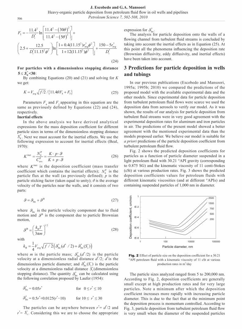
506

×

3E *

11.15rD v⎛ ⎞= ⎜ ⎟

⎝ ⎠for r* ≤ 5 or

*d

E 35 *

11.15S

D rν

− ⎛ ⎞= ⎜ ⎟⎝ ⎠

(4)

*d

E5S

D−

( ) ( )( )

22 *d

1 22 *d

*1 1 d

11 51 1ln ln2 (1 5 ) 2 1

2 110 13 tan 3 tan3 3

SF

S

S

φφφ φ

φφ− −

⎡ ⎤⎡ ⎤ ++ ⎢ ⎥= − +⎢ ⎥⎢ ⎥−⎢ ⎥ −⎣ ⎦ ⎣ ⎦

⎛ ⎞−−⎛ ⎞− ⎜ ⎟⎜ ⎟

⎝ ⎠ ⎝ ⎠

(12)

( )( )( )

2*2d

2 2 2*d

*1 1 d

11 (1 5 ) 1ln ln2 21 5 1

2 110 13 tan 3 tan3 3

SF

S

S

φφφ φ

φφ− −

⎡ ⎤⎡ ⎤ −− ⎢ ⎥= − +⎢ ⎥⎢ ⎥+⎢ ⎥ +⎣ ⎦ ⎣ ⎦

⎛ ⎞−−⎛ ⎞− ⎜ ⎟⎜ ⎟

⎝ ⎠ ⎝ ⎠

(13)

2*E 0.1923

11.4rD ν

⎛ ⎞= −⎜ ⎟

⎝ ⎠for 5 ≤ *r ≤ 30 or

*d

E 2*30 0.1923

11.4S

D rν− ⎛ ⎞

= −⎜ ⎟⎝ ⎠

(15)

*d

E30S

D−

( )( )

*d

22P P 030 4 2* 2

iavg

11.4 3011.4 11.4 ln/2 11.4

s

NC C F

DV f S

θθ

θ+

⎧ ⎫⎡ ⎤−⎪ ⎪⎢ ⎥− = −⎨ ⎬⎢ ⎥−⎪ ⎪⎣ ⎦⎩ ⎭

(21)

*d

4 *d

11.41 11.4 30. 1ln ln2 11.4 30. 2 11.4

SFSθθ

θ θ⎡ ⎤−−⎡ ⎤= − ⎢ ⎥⎢ ⎥+ +⎣ ⎦ ⎣ ⎦

(22)

( )( )

222

5 2* 2i

2 * 2 *avg avg

* 2 2 2 2 *i i

11.4 3011.4 ln11.4 5

1 0.4(11.15 ) 150 512.52.5 ln11.15 1 12(11.15 )

FD

r rD D

θ

θ

φφ φ

⎡ ⎤−= − +⎢ ⎥

−⎢ ⎥⎣ ⎦⎡ ⎤+ −⎛ ⎞

+ +⎢ ⎥⎜ ⎟ +⎢ ⎥⎝ ⎠ ⎣ ⎦

(24)

(24)

For particles with a dimensionless stopping distance


*d

P PS

C C= at * *d=r S

andP P

30C C= at * =30r ,



get:

( )( )

*d

22P P 030 4 2* 2

iavg

11.4 3011.4 11.4 ln/2 11.4

s

NC C FDV f s

θθ

θ+

⎧ ⎫⎡ ⎤−⎪ ⎪⎢ ⎥− = −⎨ ⎬⎢ ⎥−⎪ ⎪⎣ ⎦⎩ ⎭

. (21)

Such that, *d

4 *d

11.41 11.4 30. 1ln ln2 11.4 30. 2 11.4

sF

sθθ

θ θ⎡ ⎤−−⎡ ⎤= − ⎢ ⎥⎢ ⎥+ +⎣ ⎦ ⎣ ⎦

, (22)



turbulent core.



defined as *d

P P P0 avg S



avg 1 2 3 5*i

11.15 11.15/2 11.43 1.5

K V f F F F FD

φ φ θ−

⎧ ⎫= − + +⎨ ⎬

⎩ ⎭(23)



( )( )

222

5 2* 2i

2 * 2 *avg avg

* 2 2 2 2 *i i

11.4 3011.4 ln11.4 5

1 0.4(11.15 ) 150-512.52.5 ln11.15 1 12(11.15 )

FD

r rD D

θ

θ

φφ φ

⎡ ⎤−= − +⎢ ⎥

−⎢ ⎥⎣ ⎦⎡ ⎤+⎛ ⎞

+ +⎢ ⎥⎜ ⎟ +⎢ ⎥⎝ ⎠ ⎣ ⎦

(24).



{ }avg 4 5/2 / 11.4K V f F Fθ= + (25)


: By combining Equations (20) and (21) and solving for K

we get:

(25)


*d

P PS

C C= at * *d=r S

andP P

30C C= at * =30r ,



get:

( )( )

*d

22P P 030 4 2* 2

iavg

11.4 3011.4 11.4 ln/2 11.4

s

NC C FDV f s

θθ

θ+

⎧ ⎫⎡ ⎤−⎪ ⎪⎢ ⎥− = −⎨ ⎬⎢ ⎥−⎪ ⎪⎣ ⎦⎩ ⎭

. (21)

Such that, *d

4 *d

11.41 11.4 30. 1ln ln2 11.4 30. 2 11.4

sF

sθθ

θ θ⎡ ⎤−−⎡ ⎤= − ⎢ ⎥⎢ ⎥+ +⎣ ⎦ ⎣ ⎦

, (22)



turbulent core.



defined as *d

P P P0 avg S



avg 1 2 3 5*i

11.15 11.15/2 11.43 1.5

K V f F F F FD

φ φ θ−

⎧ ⎫= − + +⎨ ⎬

⎩ ⎭(23)



( )( )

222

5 2* 2i

2 * 2 *avg avg

* 2 2 2 2 *i i

11.4 3011.4 ln11.4 5

1 0.4(11.15 ) 150-512.52.5 ln11.15 1 12(11.15 )

FD

r rD D

θ

θ

φφ φ

⎡ ⎤−= − +⎢ ⎥

−⎢ ⎥⎣ ⎦⎡ ⎤+⎛ ⎞

+ +⎢ ⎥⎜ ⎟ +⎢ ⎥⎝ ⎠ ⎣ ⎦

(24).



{ }avg 4 5/2 / 11.4K V f F Fθ= + (25)

Parameters F4 and F5 appearing in this equation are the same as previously defined by Equations (22) and Parameters F4 and F

5 appearing in this equation are the

same as previously defined by Equations (22) and (24), respectively.Inertial effects

In the above analysis we have derived analytical expressions for the mass deposition coefficient for different particle sizes in terms of the dimensionless stopping distance

(24), respectively.

Inertial Effects

In the above analysis we have derived analytical expressions for the mass deposition coefficient for

different particle sizes in terms of the dimensionless stopping distance *dS . Next we must account for the

inertial effects. We use the following expression to account for inertial effects (Beal, 1970): P

iner 0Pavs

. ..

N K pKC K p

ϑϑ

= =+

, (26)

where inerK is the deposition coefficient (mass transfer coefficient which contains the inertial effects); P0N is

particle flux at the wall (as previously defined); p is the particle sticking factor (taken equal to unity); ϑ is the

average velocity of the particles near the walls, and it consists of two parts:B

fmϑ ϑ ϑ= + (27)

where fmϑ is the particle velocity component due to fluid motion and Bϑ is the component due to particle

Brownian motion, 1/2

B B

3π.k T

mϑ ⎛ ⎞= ⎜ ⎟

⎝ ⎠, (28)

( )dB avg fm fm1 2 24

** * *k V f / (d / ) (S )ϑ ϑ= +

where m is the particle mass; * *fm ( /2)dϑ is the particle velocity at a dimensionless radial distance * /2d ; *d is

the dimensionless particle diameter; and *

d

*fm ( )Sϑ is the particle velocity at a dimensionless radial distance *

dS

(dimensionless stopping distance). The quantity *fmϑ can be calculated using the following correlation

proposed by Laufer (1954): * *fm 0.05rϑ = for 0 ≤ *r ≤ 10

*fm 0.5 0.0125( 10)rϑ ∗= + − for 10 ≤ *r ≤ 30

The particles can be anywhere between * * / 2r d= and * *dr S= . Considering this we are to choose the

appropriate expression for *fmϑ .

The analysis for particle deposition onto the walls of a flowing channel from turbulent fluid streams is

concluded by taking into account the inertial effects as in Equation (25). At this point all the phenomena

influencing the deposition rate (Brownian diffusivity, eddy diffusivity, and inertial effects) have been taken

into account.

3 Predictions for particle deposition in wells and tubings In our previous publications (Escobedo J and Mansoori, 1995a; 1995b; Escobedo J and Mansoori, 2010)

we compared the predictions of the proposed model with the available experimental data and the other models.

Since experimental data for particle deposition from turbulent petroleum fluid flows were scarce we used the

. Next we must account for the inertial effects. We use the following expression to account for inertial effects (Beal, 1970):

(26)P

iner 0Pavs

N K pKC K p

ϑϑ

⋅ ⋅= =

+ ⋅ (26)

1/2B B

3πk T

mϑ ⎛ ⎞= ⎜ ⎟

⎝ ⎠(28)

with

( )*

d

* *B avg fm fm

1 2 ( 2) ( )4

*k V f / d / Sϑ ϑ= +

E *0.4D r ν= for * 30r ≥ or E30 avg *0.4

Dr

ν− = . (19)

where

(24), respectively.

Inertial Effects




iner 0Pavs

. ..

N K pKC K p

ϑϑ

= =+

, (26)




fmϑ ϑ ϑ= + (27)



B B

3π.k T

mϑ ⎛ ⎞= ⎜ ⎟

⎝ ⎠, (28)


** * *k V f / (d / ) (S )ϑ ϑ= +



d


dS



*fm 0.5 0.0125( 10)rϑ ∗= + − for 10 ≤ *r ≤ 30






into account.




is the deposition coefficient (mass transfer coefficient which contains the inertial effects);

(24), respectively.

Inertial Effects




iner 0Pavs

. ..

N K pKC K p

ϑϑ

= =+

, (26)




fmϑ ϑ ϑ= + (27)



B B

3π.k T

mϑ ⎛ ⎞= ⎜ ⎟

⎝ ⎠, (28)


** * *k V f / (d / ) (S )ϑ ϑ= +



d


dS



*fm 0.5 0.0125( 10)rϑ ∗= + − for 10 ≤ *r ≤ 30






into account.




is the particle flux at the wall (as previously defined); p is the particle sticking factor (taken equal to unity); ϑ is the average velocity of the particles near the walls, and it consists of two parts:

(27)

(24), respectively.

Inertial Effects




iner 0Pavs

. ..

N K pKC K p

ϑϑ

= =+

, (26)




fmϑ ϑ ϑ= + (27)



B B

3π.k T

mϑ ⎛ ⎞= ⎜ ⎟

⎝ ⎠, (28)


** * *k V f / (d / ) (S )ϑ ϑ= +



d


dS



*fm 0.5 0.0125( 10)rϑ ∗= + − for 10 ≤ *r ≤ 30






into account.




where

(24), respectively.

Inertial Effects




iner 0Pavs

. ..

N K pKC K p

ϑϑ

= =+

, (26)




fmϑ ϑ ϑ= + (27)



B B

3π.k T

mϑ ⎛ ⎞= ⎜ ⎟

⎝ ⎠, (28)


** * *k V f / (d / ) (S )ϑ ϑ= +



d


dS



*fm 0.5 0.0125( 10)rϑ ∗= + − for 10 ≤ *r ≤ 30






into account.




is the particle velocity component due to fluid motion and

(24), respectively.

Inertial Effects




iner 0Pavs

. ..

N K pKC K p

ϑϑ

= =+

, (26)




fmϑ ϑ ϑ= + (27)



B B

3π.k T

mϑ ⎛ ⎞= ⎜ ⎟

⎝ ⎠, (28)


** * *k V f / (d / ) (S )ϑ ϑ= +



d


dS



*fm 0.5 0.0125( 10)rϑ ∗= + − for 10 ≤ *r ≤ 30






into account.




is the component due to particle Brownian motion,

(28)

Piner 0

Pavs

N K pKC K p

ϑϑ

⋅ ⋅= =

+ ⋅ (26)

1/2B B

3πk T

mϑ ⎛ ⎞= ⎜ ⎟

⎝ ⎠ (28)

with

( )*

d

* *B avg fm fm

1 2 ( 2) ( )4

*k V f / d / Sϑ ϑ= +

E *0.4D r ν= for * 30r ≥ or E30 avg *0.4

Dr

ν− = . (19)

with

第 8 篇文章

mhγ

pmγ

h mh pmγ γ γ= +

×

第 9 篇文章

*dS

avg*d d

/2V fS S

ν

⎡ ⎤= ⎢ ⎥

⎢ ⎥⎣ ⎦ (8)

*

avg

d d/2

vr rV f

⎡ ⎤= ⎢ ⎥

⎢ ⎥⎣ ⎦

( )*

d

* *B avg fm fm

1 2 ( 2) ( )4

*k V f / d / Sϑ ϑ= +

第 16 篇

rvFgl

= (2)

* '' 'r

vFg l

= (3)

where m is the particle mass;

(24), respectively.

Inertial Effects




iner 0Pavs

. ..

N K pKC K p

ϑϑ

= =+

, (26)




fmϑ ϑ ϑ= + (27)



B B

3π.k T

mϑ ⎛ ⎞= ⎜ ⎟

⎝ ⎠, (28)


** * *k V f / (d / ) (S )ϑ ϑ= +



d


dS



*fm 0.5 0.0125( 10)rϑ ∗= + − for 10 ≤ *r ≤ 30






into account.




is the particle velocity at a dimensionless radial distance d*/2; d*is the dimensionless particle diameter; and

(24), respectively.

Inertial Effects




iner 0Pavs

. ..

N K pKC K p

ϑϑ

= =+

, (26)




fmϑ ϑ ϑ= + (27)



B B

3π.k T

mϑ ⎛ ⎞= ⎜ ⎟

⎝ ⎠, (28)


** * *k V f / (d / ) (S )ϑ ϑ= +



d


dS



*fm 0.5 0.0125( 10)rϑ ∗= + − for 10 ≤ *r ≤ 30






into account.




is the particle velocity at a dimensionless radial distance

(24), respectively.

Inertial Effects




iner 0Pavs

. ..

N K pKC K p

ϑϑ

= =+

, (26)




fmϑ ϑ ϑ= + (27)



B B

3π.k T

mϑ ⎛ ⎞= ⎜ ⎟

⎝ ⎠, (28)


** * *k V f / (d / ) (S )ϑ ϑ= +



d


dS



*fm 0.5 0.0125( 10)rϑ ∗= + − for 10 ≤ *r ≤ 30






into account.




(dimensionless stopping distance). The quantity

(24), respectively.

Inertial Effects




iner 0Pavs

. ..

N K pKC K p

ϑϑ

= =+

, (26)




fmϑ ϑ ϑ= + (27)



B B

3π.k T

mϑ ⎛ ⎞= ⎜ ⎟

⎝ ⎠, (28)


** * *k V f / (d / ) (S )ϑ ϑ= +



d


dS



*fm 0.5 0.0125( 10)rϑ ∗= + − for 10 ≤ *r ≤ 30






into account.




can be calculated using the following correlation proposed by Laufer (1954):

(24), respectively.

Inertial Effects




iner 0Pavs

. ..

N K pKC K p

ϑϑ

= =+

, (26)




fmϑ ϑ ϑ= + (27)



B B

3π.k T

mϑ ⎛ ⎞= ⎜ ⎟

⎝ ⎠, (28)


** * *k V f / (d / ) (S )ϑ ϑ= +



d


dS



*fm 0.5 0.0125( 10)rϑ ∗= + − for 10 ≤ *r ≤ 30






into account.




= 0.05r* for 0 ≤ r* ≤ 10

(24), respectively.

Inertial Effects




iner 0Pavs

. ..

N K pKC K p

ϑϑ

= =+

, (26)




fmϑ ϑ ϑ= + (27)



B B

3π.k T

mϑ ⎛ ⎞= ⎜ ⎟

⎝ ⎠, (28)


** * *k V f / (d / ) (S )ϑ ϑ= +



d


dS



*fm 0.5 0.0125( 10)rϑ ∗= + − for 10 ≤ *r ≤ 30






into account.




= 0.5r*+0.0125(r*−10) for 10 ≤ r* ≤ 30

The particles can be anywhere between r*= d*/2 and r*=

(24), respectively.

Inertial Effects




iner 0Pavs

. ..

N K pKC K p

ϑϑ

= =+

, (26)




fmϑ ϑ ϑ= + (27)



B B

3π.k T

mϑ ⎛ ⎞= ⎜ ⎟

⎝ ⎠, (28)


** * *k V f / (d / ) (S )ϑ ϑ= +



d


dS



*fm 0.5 0.0125( 10)rϑ ∗= + − for 10 ≤ *r ≤ 30






into account.




. Considering this we are to choose the appropriate

expression for

(24), respectively.

Inertial Effects




iner 0Pavs

. ..

N K pKC K p

ϑϑ

= =+

, (26)




fmϑ ϑ ϑ= + (27)



B B

3π.k T

mϑ ⎛ ⎞= ⎜ ⎟

⎝ ⎠, (28)


** * *k V f / (d / ) (S )ϑ ϑ= +



d


dS



*fm 0.5 0.0125( 10)rϑ ∗= + − for 10 ≤ *r ≤ 30






into account.




.The analysis for particle deposition onto the walls of a

flowing channel from turbulent fluid streams is concluded by taking into account the inertial effects as in Equation (25). At this point all the phenomena influencing the deposition rate (Brownian diffusivity, eddy diffusivity, and inertial effects) have been taken into account.

3 Predictions for particle deposition in wells and tubings

In our previous publications (Escobedo and Mansoori, 1995a; 1995b; 2010) we compared the predictions of the proposed model with the available experimental data and the other models. Since experimental data for particle deposition from turbulent petroleum fluid flows were scarce we used the deposition data from aerosols to verify our model. As it was shown, the results of our analysis for particle deposition from turbulent fluid streams were in very good agreement with the experimental deposition rates for aluminum and iron particles in air. The predictions of the present model showed a better agreement with the mentioned experimental data than the models proposed earlier. We believe our model is suitable for a priori predictions of the particle deposition coefficient from turbulent petroleum fluid flow.

Fig. 2 shows the predicted deposition coefficients for particles as a function of particle diameter suspended in a light petroleum fluid with 30.21 °API gravity (corresponding to 0.875 SG) and the kinematic viscosity of 11 centi-Stokes (cSt) at various production rates. Fig. 3 shows the predicted deposition coefficients values for petroleum fluids withdifferent kinematic viscosities (and at different °APIs) and containing suspended particles of 1,000 nm in diameter.

Fig. 2 Effect of particle size on the deposition coefficient for a 30.21 °API petroleum fluid with a kinematic viscosity of 11 cSt at various

production rates in m3/day

Dep

ositi

on c

oeffi

cien

t, cm

/min 1

IE-2

IE-4

IE-6

IE-8

2500

1500

750

500

200

1.91cSt

3.17cSt

4.97cSt

12.16cSt

32.12cSt

Kinematic viscosity

1001 10000 10000 2000 3000

Particle diameter, nm Oil roduction rate, m3/day

Dep

ositi

on c

oeffi

cien

t, cm

/min 1

IE-2

IE-4

IE-6

IE-8100000

The particle sizes analyzed ranged from 5 to 200,000 nm. According to Fig. 2, deposition coefficients are generally small except at high production rates and for very large particles. Note a minimum after which the deposition coefficient increases more rapidly with increasing particle diameter. This is due to the fact that at the minimum point the deposition process is momentum controlled. According to Fig. 3, particle deposition from turbulent petroleum fluid flow is very small when the diameter of the suspended particles



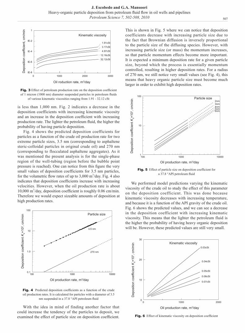
507

is less than 1,000 nm. Fig. 2 indicates a decrease in the deposition coefficients with increasing kinematic viscosity and an increase in the deposition coefficient with increasing production rate. The lighter the petroleum fluid, the higher the probability of having particle deposition.

Fig. 4 shows the predicted deposition coefficients for particles as a function of the crude oil production rate for two extreme particle sizes, 3.5 nm (corresponding to asphaltene steric-colloidal particles in original crude oil) and 270 nm (corresponding to flocculated asphaltene aggregates). As it was mentioned the present analysis is for the single-phase region of the well-tubing (region before the bubble point pressure is reached). One can notice from this figure the very small values of deposition coefficients for 3.5 nm particles, for the volumetric flow rates of up to 3,000 m3/day. Fig. 4 also indicates that deposition coefficients increase with increasing velocities. However, when the oil production rate is about 10,000 m3/day, deposition coefficient is roughly 0.06 cm/min. Therefore we would expect sizeable amounts of deposition at high production rates.

This is shown in Fig. 5 where we can notice that deposition coefficients decrease with increasing particle size due to the fact that Brownian diffusion is inversely proportional to the particle size of the diffusing species. However, with increasing particle size (or mass) the momentum increases, so that particle momentum effects become more important. It is expected a minimum deposition rate for a given particle size, beyond which the process is essentially momentum controlled, resulting in higher deposition rates. For a radius of 270 nm, we still notice very small values (see Fig. 4), this means that heavy organic particle size must become much larger in order to exhibit high deposition rates.

Fig. 3 Effect of petroleum production rate on the deposition coefficient of 1 micron (1000 nm) diameter suspended particles in petroleum fluids

of various kinematic viscosities ranging from 1.91 - 32.12 cSt

Dep

ositi

on c

oeffi

cien

t, cm

/min 1

IE-2

IE-4

IE-6

IE-8

2500

1500

750

500

200

1.91cSt

3.17cSt

4.97cSt

12.16cSt

32.12cSt

Kinematic viscosity

1001 10000 10000 2000 3000

Particle diameter, nm Oil roduction rate, m3/day

Dep

ositi

on c

oeffi

cien

t, cm

/min 1

IE-2

IE-4

IE-6

IE-8100000

Oil production rate, m3/day

Dep

ositi

on c

oeffi

cien

t Kd×

103 ,

cm/m

in

100

10

1.0

0.1

3.5 nm

270 nm

100001000100

Particle size

Fig. 4 Predicted deposition coefficients as a function of the crude oil production rates. It is calculated for particles with a diameter of 3.5

nm suspended in a 37.8 °API petroleum fluid


Dep

ositi

on c

oeffi

cien

t Kd×

103 ,

cm/m

in

100

10

1100001000100

2nm3nm4nm5nm6nm

Particle size

Fig. 5 Effect of particle size on deposition coefficient for a 37.8 °API petroleum fluid

We performed model predictions varying the kinematic viscosity of the crude oil to study the effect of this parameter on the deposition coefficient. This was done because kinematic viscosity decreases with increasing temperature, and because it is a function of the API gravity of the crude oil. Fig. 6 shows the predicted values, and we can see a decrease in the deposition coefficient with increasing kinematic viscosity. This means that the lighter the petroleum fluid is the higher the probability of having heavy organic deposition will be. However, these predicted values are still very small.


Dep

ositi

on c

oeffi

cien

t Kd×

103 ,

cm/m

in

30

20

10

0200010000

0.05cSt

0.06cSt

0.07cSt

0.04cSt

Kinematic viscosity0.03cSt

Fig. 6 Effect of kinematic viscosity on deposition coefficient

With the idea in mind of finding another factor that could increase the tendency of the particles to deposit, we examined the effect of particle size on deposition coefficient.



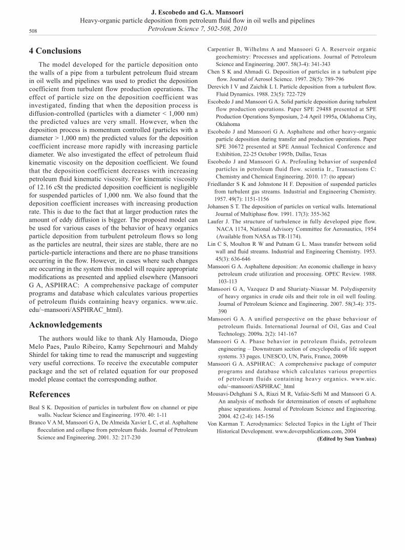
508

4 ConclusionsThe model developed for the particle deposition onto

the walls of a pipe from a turbulent petroleum fluid stream in oil wells and pipelines was used to predict the deposition coefficient from turbulent flow production operations. The effect of particle size on the deposition coefficient was investigated, finding that when the deposition process is diffusion-controlled (particles with a diameter < 1,000 nm) the predicted values are very small. However, when the deposition process is momentum controlled (particles with a diameter > 1,000 nm) the predicted values for the deposition coefficient increase more rapidly with increasing particle diameter. We also investigated the effect of petroleum fluid kinematic viscosity on the deposition coefficient. We found that the deposition coefficient decreases with increasing petroleum fluid kinematic viscosity. For kinematic viscosity of 12.16 cSt the predicted deposition coefficient is negligible for suspended particles of 1,000 nm. We also found that the deposition coefficient increases with increasing production rate. This is due to the fact that at larger production rates the amount of eddy diffusion is bigger. The proposed model can be used for various cases of the behavior of heavy organics particle deposition from turbulent petroleum flows so long as the particles are neutral, their sizes are stable, there are no particle-particle interactions and there are no phase transitions occurring in the flow. However, in cases where such changes are occurring in the system this model will require appropriate modifications as presented and applied elsewhere (Mansoori G A, ASPHRAC: A comprehensive package of computer programs and database which calculates various properties of petroleum fluids containing heavy organics. www.uic.edu/~mansoori/ASPHRAC_html).

AcknowledgementsThe authors would like to thank Aly Hamouda, Diogo

Melo Paes, Paulo Ribeiro, Kamy Sepehrnouri and Mahdy Shirdel for taking time to read the manuscript and suggesting very useful corrections. To receive the executable computer package and the set of related equation for our proposed model please contact the corresponding author.

ReferencesBea l S K. Deposition of particles in turbulent flow on channel or pipe

walls. Nuclear Science and Engineering. 1970. 40: 1-11Bra nco V A M, Mansoori G A, De Almeida Xavier L C, et al. Asphaltene

flocculation and collapse from petroleum fluids. Journal of Petroleum Science and Engineering. 2001. 32: 217-230

Car pentier B, Wilhelms A and Mansoori G A. Reservoir organic geochemistry: Processes and applications. Journal of Petroleum Science and Engineering. 2007. 58(3-4): 341-343

Che n S K and Ahmadi G. Deposition of particles in a turbulent pipe flow. Journal of Aerosol Science. 1997. 28(5): 789-796

Der evich I V and Zaichik L I. Particle deposition from a turbulent flow. Fluid Dynamics. 1988. 23(5): 722-729

Esc obedo J and Mansoori G A. Solid particle deposition during turbulent flow production operations. Paper SPE 29488 presented at SPE Production Operations Symposium, 2-4 April 1995a, Oklahoma City, Oklahoma

Esc obedo J and Mansoori G A. Asphaltene and other heavy-organic particle deposition during transfer and production operations. Paper SPE 30672 presented at SPE Annual Technical Conference and Exhibition, 22-25 October 1995b, Dallas, Texas

Esc obedo J and Mansoori G A. Prefouling behavior of suspended particles in petroleum fluid flow. scientia Ir., Transactions C: Chemistry and Chemical Engineering. 2010. 17: (to appear)

Fri edlander S K and Johnstone H F. Deposition of suspended particles from turbulent gas streams. Industrial and Engineering Chemistry. 1957. 49(7): 1151-1156

Joh ansen S T. The deposition of particles on vertical walls. International Journal of Multiphase flow. 1991. 17(3): 355-362

Lau fer J. The structure of turbulence in fully developed pipe flow. NACA 1174, National Advisory Committee for Aeronautics, 1954 (Available from NASA as TR-1174).

Lin C S, Moulton R W and Putnam G L. Mass transfer between solid wall and fluid streams. Industrial and Engineering Chemistry. 1953. 45(3): 636-646

Man soori G A. Asphaltene deposition: An economic challenge in heavy petroleum crude utilization and processing. OPEC Review. 1988. 103-113

Man soori G A, Vazquez D and Shariaty-Niassar M. Polydispersity of heavy organics in crude oils and their role in oil well fouling. Journal of Petroleum Science and Engineering. 2007. 58(3-4): 375-390

Man soori G A. A unified perspective on the phase behaviour of petroleum fluids. International Journal of Oil, Gas and Coal Technology. 2009a. 2(2): 141-167

Man soori G A. Phase behavior in petroleum fluids, petroleum engineering – Downstream section of encyclopedia of life support systems. 33 pages. UNESCO, UN, Paris, France, 2009b

Man soori G A. ASPHRAC: A comprehensive package of computer programs and database which calculates various properties of petroleum fluids containing heavy organics. www.uic.edu/~mansoori/ASPHRAC_html

Mou savi-Dehghani S A, Riazi M R, Vafaie-Sefti M and Mansoori G A. An analysis of methods for determination of onsets of asphaltene phase separations. Journal of Petroleum Science and Engineering. 2004. 42 (2-4): 145-156

Von Karman T. Aerodynamics: Selected Topics in the Light of Their Historical Development. www.doverpublications.com, 2004

(Edited by Sun Yanhua)



Heavy-organic particle deposition from petroleum fluid flow in oil

Documents