Appendix A HEAT TRANSFER DATA This appendix contains data for use with problems in the text. Data have been gathered from various primary sources and text compilations as listed in the references. Emphasis is on presentation of the data in a manner suitable for computerized database manipulation. Properties of solids at room temperature are provided in a common framework. Parameters can be compared directly. Upon entrance into a database program, data can be sorted, for example, by rank order of thermal conductivity. Gases, liquids, and liquid metals are treated in a common way. Attention is given to providing properties at common temperatures (although some materials are provided with more detail than others). In addition, where numbers are multiplied by a factor of a power of 10 for display (as with viscosity) that same power is used for all materials for ease of comparison. For gases, coefficients of expansion are taken as the reciprocal of absolute temper- ature in degrees kelvin. For liquids, actual values are used. For liquid metals, the first temperature entry corresponds to the melting point. The reader should note that there can be considerable variation in properties for classes of materials, especially for commercial products that may vary in composition from vendor to vendor, and natural materials (e.g., soil) for which variation in composition is expected. In addition, the reader may note some variations in quoted properties of common materials in different compilations. Thus, at the time the reader enters into serious profes- sional work, he or she may find it advantageous to verify that data used correspond to the specific materials being used and are up to date. 351

Welcome message from author
This document is posted to help you gain knowledge. Please leave a comment to let me know what you think about it! Share it to your friends and learn new things together.
Transcript

Appendix A
HEAT TRANSFER DATA
This appendix contains data for use with problems in the text. Data have been gathered from various primary sources and text compilations as listed in the references. Emphasis is on presentation of the data in a manner suitable for computerized database manipulation.
Properties of solids at room temperature are provided in a common framework. Parameters can be compared directly. Upon entrance into a database program, data can be sorted, for example, by rank order of thermal conductivity.
Gases, liquids, and liquid metals are treated in a common way. Attention is given to providing properties at common temperatures (although some materials are provided with more detail than others). In addition, where numbers are multiplied by a factor of a power of 10 for display (as with viscosity) that same power is used for all materials for ease of comparison. For gases, coefficients of expansion are taken as the reciprocal of absolute temperature in degrees kelvin. For liquids, actual values are used. For liquid metals, the first temperature entry corresponds to the melting point.
The reader should note that there can be considerable variation in properties for classes of materials, especially for commercial products that may vary in composition from vendor to vendor, and natural materials (e.g., soil) for which variation in composition is expected. In addition, the reader may note some variations in quoted properties of common materials in different compilations. Thus, at the time the reader enters into serious professional work, he or she may find it advantageous to verify that data used correspond to the specific materials being used and are up to date. 351

352
Appendix A
TABLE A-I Properties of Solids
p Cp k a
Material (kg/m3 (J/kg·°C) (W /m . 0c) (m2/sec) e+ O.05
Metals and Alloys Aluminum 2,707 896 204 8.418 Beryllium 1,850 825 200 5.92 Bismuth 9,780 122 7.86 0.66 Boron 2,500 1,090 30 1.1 Brass 8,522 385 111 3.41 Bronze 8,666 343 26 0.859 Cadmium 8,650 231 96.8 4.84 Carbon steel (l %C) 7,801 473 43 1.17 Cast iron 7,272 420 51.9 1.7 Chrome steel (1 %C) 7,913 448 59 1.67 Chromium 7,160 451 93.6 2.9 Cobalt 8,862 419 100 2.7 Cooper 8,954 3,831 386 11.23 Duralumin 2,787 883 164 6.676 Germanium 5,360 318 61.4 3.6 Gold 19,300 129 316 12.7 Inconel-X 8,510 439 11.6 3.1 Iron 7,870 452 81.1 2.28 Lead 11,340 129 129 2.41 Lithium 534 3,560 76 4 Magnesium 1,740 1,017 155 8.76 Manganese 7,430 477 78 2.2 Molybdenum 10,240 255 138 5.3 Nichrome 8,360 430 12.6 0.35 Nickel 8,900 442 90.5 2.3 Platinum 21,450 130 72 2.6 Silicon 2,330 691 153 9.5 Silver 10,500 235 427 17.3 Stainless steel (304) 7,900 477 14.9 3.95 Tantalum 16,600 138 57.5 2.51 Tin 5,750 227 67 5.13 Titanium 4,500 510 22 9.6 Tungsten 19,300 133 178 6.92 Uranium 19,070 116 27 1.2 Vanadium 6,100 486 33 1.1 Wrought iron 7,850 460 57.8 1.6 Zinc 7,140 388 122 4.4 Zirconium 6,570 280 22 1.2
Building Materials Bricks
Chrome 3,000 840 2.2 0.087 Common 1,600 840 0.69 0.052 Fireclay 2,000 960 1 0.052

353
Heat Transfer Data
TABLE A-I (Continued)
p Cp k II
Material (kg/nil (J/kg. 0c) (W /m . 0c) (rn2 /sec) e+o.os
Masonry 1,700 837 0.65 0.046 Concrete 2,300 880 1 0.049 Cement mortar 1,860 780 0.9 0.062
Glasses Window 2,700 800 0.84 0.039 Pyrex 2,225 835 1.4 0.D75 Plate 2,500 750 1.4 0.D75 Plaster gypsum 1,440 840 0.5 0.041
Stones Granite 2,640 800 3 0.14 Marble 2,650 1,000 2.7 0.1 Sandstone 2,200 740 2.8 0.17
Woods Fir 420 2,720 0.11 0.0096 Maple 540 2,400 0.166 0.0128 Oak 540 2,400 0.166 0.0128 Yellow pine 540 2,400 0.166 0.0128 Plywood 550 1,200 0.12 0.018
Insulating Materials Asbestos 383 816 0.113 0.036 Corkboard 160 1,900 0.043 0.014 Glass wool 40 700 0.038 0.14 Glass fiber duct liner 32 835 0.038 0.014 Glass fiber brown 16 835 0.043 0.032 Urethane 70 1,045 0.026 0.036 Vermiculite 80 835 0.068 0.01 Polystyrene (R-12) 55 1,210 0.027 0.04
Miscellaneous Materials Ice 920 2,000 2.2 0.12 Soil 2,050 1,840 0.52 0.014 Rubber, hard 1,150 2,009 0.163 0.0062 Paper 930 1,340 0.18 0.014 Diamond, Type IIa 3,500 510 2500 140 Diamond, Type lIb 3,250 510 1350 81 Silicon carbide 3,180 675 490 23 Aluminum oxide 3,970 765 39.5 1.3 Oay 1,460 880 1.3 0.1 Cotton 80 1,300 0.06 0.058

354
Appendix A
TABLEA-2 Properties of Gases
a !l- v T p cp k (m2/sec) (kg/m' sec) (m2/sec)
Name (OK) (kg/of) (J/kg· OK) (W/m· OK) (X105) (X 105) (X 105) Pr p
CO2 200 2.68 759 0.0095 0.467 l.02 0.381 0.814 0.005 250 2.15 806 0.0129 0.744 1.26 0.586 0.79 0.004 300 l.79 852 0.0166 l.09 1.5 0.838 0.763 0.0033 350 1.53 897 0.0205 l.49 1.73 1.13 0.755 0.0028 400 1.34 939 0.0244 l.94 1.94 1.45 0.747 0.0025 450 1.19 979 0.0283 2.43 2.15 l.8 0.743 0.0022 500 1.07 1,017 0.0323 2.96 2.35 2.19 0.74 0.00202 600 0.894 1,077 0.0403 4.18 2.72 3.04 0.727 0.0016 700 0.767 1,126 0.0487 5.64 3.06 3.99 0.708 0.00143 800 0.671 1,169 0.056 7.14 3.39 5.05 0.708 0.00125 900 0.596 1,205 0.0621 8.65 3.89 6.19 0.716 0.00111
1,000 0.537 1,235 0.068 10.3 3.97 7.4 0.721 0.001 Argon 200 2.44 524 0.0124 0.973 l.6 0.657 0.674 0.005
250 l.95 522 0.0152 l.49 l.95 1 0.672 0.004 300 l.62 522 0.0177 2.07 2.27 l.4 0.669 0.003333 350 1.39 521 0.0201 2.78 2.57 l.85 0.666 0.002857 400 1.22 521 0.0223 3.52 2.85 2.34 0.665 0.0025 450 l.08 521 0.0244 4.33 3.12 2.88 0.665 0.002222 500 0.974 521 0.0264 5.2 3.37 3.45 0.664 0.002 600 0.812 521 0.0301 7.12 3.82 4.72 0.662 0.001666 700 0.696 521 0.0336 9.68 4.25 6.11 0.658 0.001428 800 0.609 521 0.0369 11.6 4.64 7.62 0.655 0.00125 900 0.541 521 0.0398 14.1 :i.01 9.26 0.654 0.001111
1,000 0.487 521 0.0427 16.8 5.35 11 0.652 0.001 Ammonia 200 l.04 2,199 0.0153 0.67 0.689 0.663 0.99 0.005
250 0.831 2,248 0.0197 l.05 0.853 1.03 0.973 0.004 300 0.692 2,298 0.0246 1.55 1.03 1.48 0.959 0.0033 350 0.593 2,349 0.0302 2.17 1.21 2.03 0.938 0.0028 400 0.519 2,402 0.0364 2.92 1.39 2.68 0.917 0.0025 450 0.461 2,455 0.0433 3.82 1.58 3.42 0.894 0.0022 500 0.415 2,507 0.0506 4.86 1.76 4.25 0.8,73 0.002 550 0.378 2,559 0.058 6 1.95 5.16 0.86 0.0018 600 0.346 2,611 0.0656 7.26 2.14 6.18 0.852 0.0016 700 0.297 2,710 0.0811 10.1 2.51 8.45 0.839 0.0014 800 0.26 2,810 0.0977 13.4 2.88 11.1 0.828 0.0012 900 0.231 2,907 0.1146 17.1 3.24 14 0.822 0.0011
1,000 0.208 3,001 0.1317 21.1 3.59 17.3 0.818 0.001 Air 100 3.6 1,027 0.00925 0.25 0.692 0.192 0.77 0.Dl08
150 2.37 1,010 0.0137 0.575 1.03 0.434 0.753 0.0066 200 1.77 1,003 0.0181 1.02 1.34 0.757 0.74 0.005 250 1.41 1,003 0.0223 1.57 1.61 1.14 0.724 0.004 300 1.18 1,005 0.0261 2.21 1.85 1.57 0.712 0.00333 350 1.01 1,008 0.0297 2.92 2.08 2.06 0.706 0.00286 400 0.883 1,013 0.0331 3.7 2.29 2.6 0.703 0.00251 450 0.785 1,020 0.0363 4.54 2.49 3.18 0.7 0.00225

355
Heat Transfer Data
TABLE A-2 (Continued)
a ,. • T p Cp k (m2 jsec) (kgjm . sec) (m2 jsec)
Name (OK) (kgjof) (Jjkg·oK) (Wjm·oK) (X105) (X 105) (X105) Pr p
Air 500 0.706 1,029 0.0395 5.44 2.68 3.8 0.699 0.002 550 0.642 1,039 0.0426 6.39 2.86 4.45 0.698 0.00187 600 0.589 1,051 0.0456 7.37 3.03 5.15 0.698 0.00167 650 0.543 1,063 0.0484 8.38 3.19 5.88 0.701 0.00154 700 0.504 1,075 0.0513 9.46 3.35 6.64 0.702 0.0014 750 0.471 1,087 0.0541 10.6 3.5 7.43 0.703 0.0013 800 0.441 1,099 0.0569 11.7 3.64 8.25 0.704 0.00123 850 0.415 1,110 0.0597 13 3.78 9.11 0.704 0.00118 900 0.392 1,120 0.0625 14.2 3.92 9.99 0.705 0.001ll 950 0.372 I,m 0.0649 15.4 4.05 10.9 0.706 0.00105
1,000 0.353 1,141 0.0672 16.7 4.18 11.8 0.709 0.001 1,100 0.321 1,159 0.0717 19.3 4.42 13.8 0.716 0.0009 12,00 0.294 1,175 0.0759 22.2 4.65 15.8 0.72 0.00083 1,300 0.272 1,189 0.0797 24.7 4.88 18 0.729 0.00076
Helium 250 0.244 5,197 0.115 9.06 1.5 6.15 0.676 0.005 250 0.195 5,197 0.134 15.4 1.75 8.97 0.68 0.004 300 0.163 5,197 0.15 17.7 1.99 12.2 0.69 0.00352 350 0.139 5,197 0.165 22.8 2.21 15.9 0.698 0.0028 400 0.122 5,197 0.18 28.3 2.43 19.9 0.703 0.0025 450 0.109 5.197 0.195 34.5 2.63 24.3 0.702 0.0022 500 0.0976 5.197 0.211 41.7 2.83 29 0.695 0.002 600 0.0813 5.197 0.247 58.4 3.2 39.3 0.673 0.00167 700 0.0697 5.197 0.278 76.7 3.55 50.9 0.663 0.0014 800 0.061 5.197 0.307 96.8 3.88 63.7 0.657 0.00125 900 0.0542 5.197 0.335 119 4.2 77.5 0.652 0.001ll
1.000 0.0488 5.197 0.363 143 4.5 92.3 0.645 0.001 Hydrogen 200 0.123 13,450 0.128 7.69 0.681 5.54 0.717 0.005
250 0.0983 14.070 0.156 11.3 0.789 8.03 0.713 0.004 300 0.0819 14.320 0.182 15.5 0.896 10.9 0.705 0.003333 350 0.0702 14,420 0.203 20.1 0.988 14.1 0.705 0.002857 400 2.0614 14,480 0.221 24.9 1.09 17.8 0.714 0.0025 450 0.0546 14.500 0.239 31.2 1.18 21.7 0.719 0.002222 500 0.0492 14.510 0.256 35.9 1.27 25.9 0.721 0.002 600 0.041 14.540 0.291 48.9 1.45 35.4 0.724 0.001666 700 0.0351 14,610 0.325 63.4 1.61 45.9 0.724 0.001428 800 0.0307 14,710 0.36 79.7 1.77 57.6 0.723 0.00125 900 0.0273 14.840 0.394 108 1.92 70.3 0.723 0.001ll1
1.000 0.0246 14.990 0.428 116 2.07 84.2 0.724 0.001 Watervapor 400 0.555 2.000 0.0264 2.38 1.32 2.38 1 0.0025
450 0.491 1.968 0.0307 3.17 1.52 3.1 0.974 0.0022 500 0.441 1,977 0.0357 4.09 1.73 3.92 0.958 0.002 600 0.367 2,022 0.0464 6.25 2.13 5.82 0.928 0.00167 700 0.314 2.083 0.0572 8.74 2.54 8.09 0.925 0.0014 800 0.275 2.148 0.0686 11.6 2.95 10.7 0.924 0.00125 900 0.244 2.217 0.0779 14.4 3.36 13.7 0.956 0.001ll
1.000 0.22 2,288 0.0871 17.3 3.76 17.1 0.988 0.001

356
Appendix A
TABLEA-3 Properties of Liquids
a p. • T p Cp k (rn2/sec) (kgfrn'sec) (m>/sec)
Name (OK) (kgfni') J/kg· OK) (W/rn· OK) (XI0s) (XI0s) (XlOs) Pr fJ
Ethylene glycol 273 1,131 2,294 0.242 0.00933 6,510 5.76 617 0.00065 280 1,129 2,323 0.244 0.00933 4,200 3.73 400 0.00065 300 l,lJl 2,415 0.252 0.000936 1,570 1.41 151 0.00065 320 1,096 2,505 0.258 0.00094 757 0.691 73.5 0.00065 340 1,084 2,592 0.261 0.000929 431 0.398 42.8 0.00065 350 1,079 2,637 0.261 0.000917 342 0.317 34.6 0.00065 360 1,074 2,682 0.261 0.00906 278 0.259 28.6 0.00065
Freon-12 240 1,498 892 0.069 0.00516 38.5 0.0257 5.9 0.0019 250 1,470 904 0.07 0.00527 35.4 0.0241 4.6 0.002 260 1,439 916 0.073 0.00554 32.2 0.0224 4 0.0021 273 1,393 935 0.073 0.00559 29.8 0.0214 3.8 0.00236 280 1,374 945 0.073 0.00562 28.3 0.0206 3.7 0.00235 300 1,306 978 0.072 0.00564 25.4 0.0195 3.5 0.00275 320 1,229 1,016 0.068 0.00545 23.3 .0.019 3.5 0.0035
Glycerin 273 1,276 2,261 0.282 0.00977 1,060,000 831 85,000 0.0004 280 1.272 2,298 0.284 0.00972 534,000 420 43,200 0.00047 300 1.260 2,427 0.286 0.00955 79.900 63.4 6,780 0.00048 320 1,247 2,564 0.287 0.00897 21,000 16.8 1,870 0.0005
Water 273 1,000 4,217 0.564 0.0134 175 0.179 13 -0.00006 280 1,000 4,198 0.582 0.0139 142 0.142 10.3 0.000046 300 997 4,179 0.613 0.0147 85.5 0.0861 5.83 0.000114 320 989 4,180 0.64 0.0155 57.7 0.0583 3.77 0.00043 340 979 4,188 0.66 0.0161 42 0.0429 2.66 0.00056 350 974 4,195 0.668 0.0164 36.5 0.0375 2.29 0.00062 360 967 4,203 0.674 0.0166 32.4 0.0335 2.02 0.000698 373 958 4,217 0.68 0.0168 27.9 0.0291 1.76 0.00075 380 953 4,226 0.683 0.017 26 0.0273 1.61 0.00078 400 937 4,256 0.688 0.0173 21.7 0.0232 1.34 0.00089
Engine oil (unused) 273 899 1,796 0.147 0.0091 385,000 428 47,000 0.00065
280 895 1,827 0.145 0.0088 217,000 243 27,500 0.00065 300 884 1,909 0.145 0.00859 48,600 55 6,400 0.00066 320 872 1,993 0.143 0.00823 14,100 16.1 1.965 0.00066 340 860 2,076 0.139 0.00779 5,310 6.17 793 0.00068 350 854 2,118 0.138 0.00763 3.560 4.17 546 0.00068 360 848 2,161 0.138 0.00753 2,520 2.97 395 0.00069 380 836 2,250 0.136 0.00723 1,410 1.69 233 0.0007 400 825 2,337 0.134 0.00695 874 1.06 152 0.0007
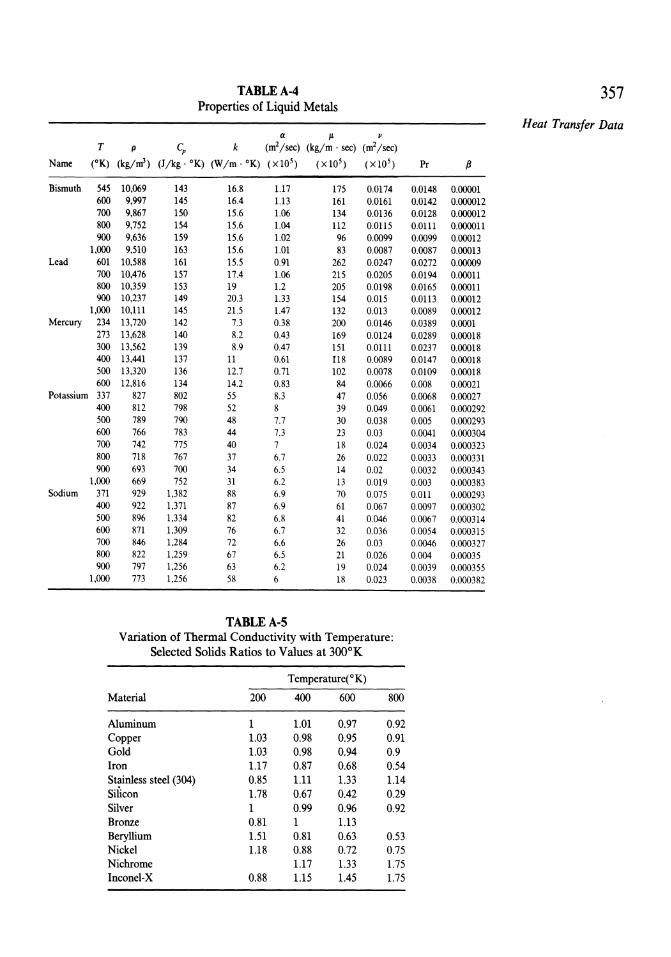
TABLEA-4 357 Properties of Liquid Metals
Heat Transfer Data a p. v
T p Cp k (m2 jsec) (kgjm· sec) (m2jsec)
Name ("K) (kg/oi) (Jjkg· OK) (Wjm· OK) (X10s) (X 105) (X 105) Pr ft
Bismuth 545 10,069 143 16.8 1.17 175 0.0174 0.0148 0.00001 600 9,997 145 16.4 1.13 161 0.0161 0.0142 0.0000l2 700 9,867 150 15.6 1.06 134 0.0136 0.0l28 0.000012 800 9,752 154 15.6 1.04 112 0.0115 0.0111 0.000011 900 9,636 159 15.6 1.02 96 0.0099 0.0099 0.00012
1,000 9,510 163 15.6 1.01 83 0.0087 0.0087 0.00013 Lead 601 10,588 161 15.5 0.91 262 0.0247 0.0272 0.00009
700 10,476 157 17.4 1.06 215 0.0205 0.0194 0.00011 800 10,359 153 19 1.2 205 0.0198 0.0165 0.00011 900 10,237 149 20.3 1.33 154 0.015 0.0113 0.00012
1,000 1O,lll 145 21.5 1.47 132 0.013 0.0089 0.00012 Mercury 234 13,720 142 7.3 0.38 200 0.0146 0.0389 0.0001
273 13,628 140 8.2 0.43 169 0.0124 0.0289 0.00018 300 13,562 139 8.9 0.47 151 0.0111 0.0237 0.00018 400 13,441 137 11 0.61 tI8 0.0089 0.0147 0.00018 500 13,320 136 l2.7 0.71 102 0.0078 0.0109 0.00018 600 12,816 134 14.2 0.83 84 0.0066 0.008 0.00021
Potassium 337 827 802 55 8.3 47 0.056 0.0068 0.00027 400 812 798 52 8 39 0.049 0.0061 0.000292 500 789 790 48 7.7 30 0.038 0.005 0.000293 600 766 783 44 7.3 23 0.03 0.0041 0.000304 700 742 775 40 7 18 0.024 0.0034 0.000323 800 718 767 37 6.7 26 0.022 0.0033 0.000331 900 693 700 34 6.5 14 0.02 0.0032 0.000343
1,000 669 752 31 6.2 13 0.019 0.003 0.000383 Sodium 371 929 1,382 88 6.9 70 0.075 0.011 0.000293
400 922 1,371 87 6.9 61 0.067 0.0097 0.000302 500 896 1,334 82 6.8 41 0.046 0.0067 0.000314 600 871 1.309 76 6.7 32 0.036 0.0054 0.000315 700 846 1,284 72 6.6 26 0.03 0.0046 0.000327 800 822 1,259 67 6.5 21 0.026 0.004 0.00035 900 797 1,256 63 6.2 19 0.024 0.0039 0.000355
1,000 773 1,256 58 6 18 0.023 0.0038 0.000382
TABLEA-5 Variation of Thermal Conductivity with Temperature:
Selected Solids Ratios to Values at 3000 K
TemperatureeK)
Material 200 400 600 800
Aluminum 1 1.01 0.97 0.92 Copper 1.03 0.98 0.95 0.91 Gold 1.03 0.98 0.94 0.9 Iron 1.17 0.87 0.68 0.54 Stainless steel (304) 0.85 1.11 1.33 1.14 Silicon 1.78 0.67 0.42 0.29 Silver 1 0.99 0.96 0.92 Bronze 0.81 1 1.13 Beryllium 1.51 0.81 0.63 0.53 Nickel 1.18 0.88 0.72 0.75 Nichrome 1.17 1.33 1.75 Inconel-X 0.88 1.15 1.45 l.75

358
Appendix A
TABLEA-6 Surface Tension for Selected Liquids Evaluated as C1 - C2 (T - 273) with
Temperature in Degrees Kelvin
Material C1(N/m)(XI03) C2(N/m· oK)(x103)
Acetone 26.26 0.112 Ethanol 24.05 0.0832 Methanol 24 0.0773 Ammonia 23.41 0.2993 Ethylene glycol 50.21 0.089 Mercury 490.6 0.2049 Water 75.83 0.1477
TABLEA-7 Selected Boiling Data at 1 Atmosphere
hlg
T.at (J/kg) p-liq p-vap C1
Fluid (OK) (Xl0- 3) (kg/ni') (kg/ni') (N/m)( x 103)
Ethanol 351 846 757 1.44 17.7 Freon-12 243 165 1,488 6.32 15.8 Mercury 630 301 12,740 3.9 417 Water 373 2,257 958 0.6 58.6 Ammonia 240 1,371 683 0.89 33.3
TABLEA-8 Typical Emmissivities at 3000 K
Aluminum, polished 0.04 Aluminum, anodized 0.8 Chronrium,polished 0.1 Copper, polished 0.03 Gold, polished 0.03 Gold, bright foil 0.07 Iron, polished 0.05 Iron, cast 0.4 Iron, rusted 0.6 Lead, polished 0.06 Lead, oxidized 0.6 Silver, polished 0.02 Steel, stainless polished 0.2 Steel, oxidized 0.8 Asphalt 0.9 Brick, common 0.95 Concrete 0.9 Glass, window 0.9 Glass, Pyrex 0.8 Wood 0.9 Paints 0.9 Paper 0.95 Sand 0.9 Skin 0.95 Soil 0.95 Rubber 0.9

TABLEA-9 359 Conversion Factors
Metric English Heat Transfer Data
Values Units Values Units
Acceleration 1 m/sec' 3.2808 ftjsec2
0.3048 1 Area 1 m2 10.764 ft2
0.0929 1 Density 1 kg/m3 0.06243 Ibm/ft3
16.02 1 Thermal dilfusivity 1 m2 10.764 ft2
0.0929 1 Energy 1 0.000948 Btu
1055 1 1 cal 0.003968 Btu
252 1 Force 1 N 0.2248 Ib
4.448 1 Heat transfer coefficient 1 W/m2 . oK 0.176 Btu/hr· ft2 . R
5.667 1 Kinematic viscosity (p) 1 m2/sec 10.764 ft 2/sec
0.0922 1 Heat flux 1 W/m2 0.3171 Btu/hr· ft2
0.3154 1 Length 1 m 3.281 ft
0.3048 1 Mass 1 kg 2.205 Ibm
0.454 1 Pressure 1 N/nr (pascal) 0.0209 Ib/ft2
1 0.000145 psi 6895 1 psi
47.88 1 Ib/ft2
Specific heat 1 J/kg. OK 0.000239 Btu/Ibm· R 4187 1
Temperature 1 OK (kelvin) 1 R (Rankine) 9
1 (460 + OF) 9
1.8 1 R
1 °C (Centigrade) 1 CF - 32) 9
Thermal conductivity 1 W/m. OK 0.578 Btu/hr· ft . R 1.73 1 0.413 cal/sec . m . kg 1 1 cal/sec . m . kg 2.42
Viscosity (p. ) 1 kg/m'sec 0.672 Ibm/ft· sec 1.488 1 1 g/ cm . sec (poise) 0.0672
14.88 1 Volume 1 m3 35.315 ft3
0.02832 1 1 Liter 0.03515
28.32 Liters 1 ft3
1 0.264 gal (U.S.) 3.758 1 gal (U.S.)

360
Appendix A
TABLEA-IO Physical Constants
Acceleration of gravity, sea level Atmospheric pressure Gas constant Speed of light Stefan-Boltzmann constant Planck's constant Boltzmann's constant
REFERENCES
9.81 101330
8315 3.0E + 08
5.669E - 8 6.625E - 34 1.4 X 10- 23
m/sec2
N/m2 J/kg . mole· oK m/sec W/m2 • OK
J . sec J/oK
1. E. R. G. Eckert and R. M. Drake, Analysis of Heat and Mass Transfer, McGraw-Hill, New York,1972.
2. C. Y. Ho, R. W. Powell, and P. E. Liley, "Thermal Conductivity of the Elements: A Comprehensive Review," J. Phys. Chern. Ref. Data, 3, Suppl. 1, 1974.
3. J. P. Holman, Heat Transfer, 5th ed., McGraw-Hill, New York, 1981. 4. F. P. Incoprera and D. P. DeWitt, Introduction to Heat Transfer, Wiley, New York, 1985. 5. T. F. Irvine, Jr. and J. P. Hartnett (eds.), Steam and Air Tables in S.I. Units, Hemisphere,
Washington, DC, 1976. 6. 1. 1. Jasper, "The Surface Tension of Pure Liquid Compounds," J. Phys. Chern. Ref. Data,
1, 841 (1972). 7. 1. H. Keenan, F. G. Keyes, P. G. Hill, and J. G. ~oore, Steam Tables, Wiley, New York,
1969. 8. J. Lienhard, A Heat Transfer Textbook, Prentice-Hall, Englewood Cliffs, NJ, 1981. 9. Y. S. Touloukian and C. Y. Ho (eds.), Thermophysical Properties of Matter, Plenum, New
York, Vols. 1-13,1970-1977. 10. U.S. Department of Commerce, "Tables of Thermodynamic Properties of Ammonia,"
Bureau of Standards Circular No. 142, 1945. 11. N. B. Vargaftik, Tables on the Thermophysical PropertIes of Liquids and Gases, 2nd ed.,
Hemisphere, Washington, DC, 1975. 12. J. T. R. Watson, R. S. Basa, and J. V. Sengers, "An Improved Representative Equation for
the Dynamic Viscosity of Water Substance," J. Phys. Chern. Ref. Prop., 9, 1255 (1980). 13. F. White, Heat Transfer, Addison-Wesley, Reading, MA, 1984.

AppendixB
MATHEMATICAL APPENDIXES
B-1. BESSEL FUNCflONS
The Bessel equation, which occurs frequently in dealing with problems in cylindrical geometry, can be presented in the form
(B-1)
One also may encounter an alternate form
(B-2)
The differential equation may be solved in terms of an infinite series. Two independent solutions are found as a function of z = Hr. One is
. 1 (z)n[ (z/2)2 (Z/2)4 1 In(z) = -;;T 2" 1 - l!(n + 1) + 2!(n + l)(n + 2) - ... (B-3)
361

362 Appendix B
The other may be cast in the form
2 [ Z 1 n 1 1 1 n-l (n - m - 1)! Yn(z)=-ln-+y+- L - In(z)-- L n-2m
7T 2 2 m=l m 7T m=O m!(z/2)
100 m (z/2r+ 2m m (1 1) - -t L (-1) L - +-
7T m=l mIen + m)! p=l P P + n
y = 0.57722 (B-4)
These two solutions are referred to as ordinary Bessel functions of the first and second kind. Tabulated values are given in Table B-1-I.
For large values of z, the Bessel functions become
(B-S)
Y(z) "'" Ii Sin[z - ~(n + ~)] n TTZ • 2 2
(B-6)
Thus, the Bessel function have characteristics analogous to the sine and cosine solutions of plane geometry problems.
We may use orthogonality properties of the Bessel functions to construct the analogue of Fourier series. There will be a set of values Bm for which JO(BmR) will vanish. We note the orthogonality relationship
p=m
p=fom
(B-7)
Table B-1-2 contains zeros of the Bessel functions. The spacing between zeros tends toward 7T in keeping with Eqs. (B-5) and (B-6). Another useful relationship is
(B-8)
These relationships can be combined to yield coefficients of series expansions as in Chapter 4. We also note derivative relationships:
dlo - = -J (z) dz 1
(B-9)
n>O (B-10)

TABLEB-l-l 363 Bessel Functions
Mathematical A. Ordinary Bessel Functions Appendixes
Z lo(z) Ij(z) Yo(z) Yj(z)
0 1.0 0.0 -00 -00
0.2 0.9975 0.0995 -1.0811 - 3.3238 0.4 0.9604 0.1960 -0.6060 -1.7809
0.6 0.9120 0.2867 -0.3085 -1.2604
0.8 0.8463 0.3088 -0.0868 -0.9781
1.0 0.7652 0.4401 0.0883 -0.7812 1.2 0.6711 0.4983 0.2281 -0.6211 1.4 0.5669 0.5419 0.3379 -0.4791
1.6 0.4554 0.5699 0.4204 -0.3476 1.8 0.3400 0.5815 0.4774 -0.2237 2.0 0.2239 0.5767 0.5104 -0.1070 2.2 0.1104 0.5560 0.5208 0.0015 2.4 0.0025 0.5202 0.5104 0.1005 2.6 -0.0968 0.4708 0.4813 0.1884 2.8 -0.1850 0.4097 0.4359 0.2635 3.0 -0.2601 0.3391 0.3769 0.3247 3.2 -0.3202 0.2613 0.3071 0.3101 3.4 -0.3643 0.1792 0.2296 0.4010 3.6 -0.3918 0.0955 0.1477 0.4154 3.8 -0.4026 0.0128 0.0645 0.4141 4.0 -0.3971 -0.0660 -0.0169 0.3979
B. Modified Bessel Functions
e-'/o(z) e-'/j(z) I(z)/Io(z) e'Ko(z) e'Kj(z)
0 1.0 0.0 0.0 00 00
0.2 0.8269 0.0823 0.0995 2.1408 5.8334 0.4 0.6974 0.1368 0.1962 1.6627 3.2587 0.6 0.5993 0.1722 0.2873 1.4167 2.3739 0.8 0.5241 0.1945 0.3711 1.2582 1.9179 1.0 0.4658 0.2079 0.4463 1.145 1.6362 1.2 0.4198 0.2153 0.5129 1.0575 1.4429 1.4 0.3831 0.2185 0.5703 0.9881 1.3011 1.6 0.3533 0.2190 0.6170 0.9309 1.1919 1.8 0.3289 0.2177 0.6619 0.8828 1.1048 2.0 0.3085 0.2153 0.6979 0.8416 1.0335 2.2 0.2913 0.2121 0.7281 0.8057 0.9738 2.4 0.2766 0.2085 0.7538 0.7740 0.9929 2.6 0.2639 0.2047 0.7757 0.7459 0.8790 2.8 0.2528 0.2007 0.7939 0.7206 0.8405 3.0 0.2430 0.1968 0.8099 0.6978 0.8067 3.2 0.2343 0.1930 0.8237 0.6770 0.7763 3.4 0.2264 0.1892 0.8315 0.6580 0.7491 3.6 0.2193 0.1856 0.8463 0.6405 0.7245 3.8 0.2129 0.1821 0.8553 0.6243 0.7021 4.0 0.2070 0.1788 0.8638 0.6093 0.6816 4.5 0.1942 0.1710 0.8805 0.5761 0.6371 5.0 0.1835 0.1640 0.8937 0.5478 0.6002 6.0 0.1667 0.5521 0.9124 0.5019 0.5422 7.5 0.1483 0.1380 0.9305 0.4505 0.4797 10.0 0.1278 0.1213 0.9491 0.3916 0.4108 15.0 0.1039 0.1004 0.9663 0.3210 0.3315 20.0 0.0898 0.0875 0.9744 0.2785 0.2854 25.0 0.0800 0.6785 0.9788 0.1407 0.1435

364 Appendix B
A variation on the Bessel equation is
(B-11)
This is called the modified Bessel equation and yields solutions called modified Bessel functions, which may be expressed as (with Z = Br)
1 (Z )n[ (Z/2)2 (Z/2)4 1 In(z) = n! 2 1 + l!(n + 1) + 2!(n + l)(n + 2) + ... (B-12)
Kn(z) = (-1) In - + y - - I: - In(z) n+l[ (Z) 1 n 1] 2 2 m=l m
1 n - 1 m(n-m-1)! + - ~ (-1)
2 m~l m!(z/2r-2m
m1 00 (z/2r+ 2m m (1 1) +(-1) -I: I: -+-
2 m=O m!(m + n)! p=l P P + n (B-13)
These functions are analogues of exponentials, and, for large values of z, behave as
(B-14)
(B-15)
TABLEB-1-2 Zeros of the Bessel Functions
Jo J1
2.4048 3.8317 5.5201 7.0156 8.6537 10.1735
11.7915 13.3237 14.9309 16.4706 18.0711 19.6159 21.2116 22.7601 24.3525 25.9037 27.4935 29.0468 30.6346 32.1897

Note that for large values of z, the ratio encountered in efficiency of triangular fins goes to
I1{z) 1 - 3/8z 1 Io(z) = 1+1/8z ::::1- 2z (8-16)
Thus, we see that this ratio goes to 1 as z gets large. We note that derivatives are given by
(8-17)
(8-18)
(8-19)
(8-20)
For the purpose of evaluation of Bessel functions on a computer, expressions other than the set of infinite series given above may be used. Convenient algorithms that may be used on a personal computer are given in Table B-1-3. These algorithms have accuracies on the order of 10- 7 or better, which is why the coefficients are given with many significant figures.
The algorithms in Table B-1-3 can be evaluated easily in a subroutine in FORTRAN or BASIC. This single subroutine can then be available for incorporation into any of several computer projects suggested in the text. For those using spreadsheets on a personal computer, a sample spreadsheet is given in Table B-1-4 for evaluating the Jo Bessel function. Once saved, this spreadsheet can be used as an ingredient within other spreadsheets that require the Bessel function. The spreadsheet provides for evaluation using low-argument and high-argument values and chooses the proper Bessel function evaluation depending on whether the statement B2 > 3 (and, therefore, the result in B38) is TRUE or FALSE. Similar columns can be prepared for the other Bessel functions.
In working with this sample spreadsheet, the reader will observe that if moderate accuracy is acceptable, then fewer terms in the series may be taken. Since this and other Bessel functions can occur in a variety of problems (fins, multidimensional heat conduction, time-dependent heat conduction), it may be worthwhile to spend a little extra typing effort to put in the whole series. The student should get accustomed to the idea of making judgments about how much effort to devote to obtain how much accuracy.
365 Mathematical
Appendixes

366 TABLE B-I-3 Convenient Algorithms for Computer Evaluation
Appendix B of Bessel Functions
A. Jo(z) (1) z ~ 3 1 = zj3
Jo(z) = 1 - 2.2499997/2 + 1.265620814
- 0.3163866/6 + 0.0444479/8 - 0.0039444/10
+ 0.0002100/12
(2) z ~ 3 u = 3jz locos80
Jo ( z) = ----rz-10 = 0.79788456 - 0.OOOOOO77u - 0.00552740u2
- 0.00009512u3 + 0.00137237u4
- 0.0072805u5 + 0.00014476u6
8 0 = z - 0.78539816 - 0.04166397u - 0.00003954u 2
+ 0.00262573u3 - 0.00054125u4 - 0.00029333u5
+ 0.00013555u6
B. J1(z) (1) z ~ 3 1 = zj3
~Jl(Z) = 0.5 - 0.56249985/2 + 0.2109357314
- 0.03954289/6 + 0.00443319t8 - 0.00031761/10
- 0.00001109/12
(2) z ~ 3 u = 3jz 80
J1(z) = 10 cos r; 11 = 0.79788456 + 0.OOOOO156u + 0.01659667u2
+ 0.00017105u3 - 0.OO249511u 4
+ 0.OO113653u5 - 0.0002oo33u6
8 1 = Z - 2.35619449 + 0.12499612u + 0.00005650u2 - 0.00537879u3
+ 0.00074348u4 + 0.00079824u5
- 0.00029166u6
C. Yo(z) (1) z ~ 3 1 = zj3
Yo(z) = ~ In( ~) Jo(z) + 0.36746691
(2) z ~ 3
+ 0.60559366/2 - 0.7435038414 + 0.25300117/6
- 0.042612118 + 0.00427916/10 - 0.00024846112
10 sinh 8 0 Yo(z) = r;
D. Y1(z) (1) z ~ 3 1 = zj3
zY1(z) = ~z In( ~ )J1(Z) - 0.6366198 + 0.2212091/2
+ 2.1682709/4 - 1.316482716 + 0.3123951t8
- 0.0400976/10 + 0.0027873/12
(2) z ~ 3 11 sin 8 1
Y1 (z) = ----rz-E. Io(z) (1) z ~ 3 Y = zj3
Io(z) = 1 + 3.5156229y 2 + 3.0899424y 4 + 1.2067492 y 6
+ 0.2659732 y 8 + 0.0360768y1O + 0.0045813i2

TABLE B·l·3 (Continued)
(2) z> 3.75 x = 3.75/z
{ie-Zlo(z) = 0.39894228 + 0.01328592x + 0.00225319x 2
F. II(z)
+ 0.00157565x3 + 0.00916281x4 - 0.02057706x5
+ 0.02635537x6 - 0.01647633x7 + 0.00392377x8
(1) Z s 3.75 y = z/3.75
II (z) = 0.5 + 0.87890594y 2 + 0.51498869y 4 z
+ 0.15084934y6 + 0.02658733y 8
+ 0.00301532 y lO + 0.00032411y12 (2) z> 3.75 x = 3.75/x
{i e - Z II (z) = 0.39894228 - 0.03988024x
G. Ko(z)
- 0.00362018x2 + 0.00103801x3 - 0.01031555x4 + 0.02282967x5 - 0.02895312x6 + 0.01787654x7
- 0.00420059x8
(1) z s 2 v = z/2
Ko(z) = - In( ~) Io(z) - 0.57721566 + 0.42278420v2
+ 0.23069756v4 + 0.03488590v6 + 0.002626698v8
+ 0.0010750vlo + 0.OOOOO740z12
(2) z ~ 2 w = 2/z
{i eZKo(z) = 1.25331414 - 0.07832358w + 0.02189568w 2
H. KI(z)
- 0.01062446w3 + 0.00587872w4 - 0.002515400w 5
+ 0.00053208w6
(1) z s 2 v = z/2
zKI(z) = z In( ~) II(z) + 1 + 0.15443144v2
- 0.67278579v4 - 0.18156897v6 - 0.019l9402v8
- 0.00110404vlO - 0.00004686v12
(2) z ~ 3 w = 2/z
{iezKI(z) = 1.25331414 + 0.23498619w
1 2 3 4 5 6 7 8 9 10
- 0.03655620w 2 + 0.01504268w3 - 0.00780353w 4
+ 0.00325614w5 - 0.00068245w6
TABLEB·l·4 Spreadsheet for Evaluation of 10
A
JO BESSEL ARGUMENT CASE 1 DIVIDED BY FIRST TERM NEXT TERM NEXT TERM NEXT TERM NEXT TERM NEXT TERM
3
B
FUNCTION ENTER VALUE ARGUMENT < 3 + B2/3 1 -2.2499997 * (B4 A 2) 1.265208 * (B4 A 4) -.3163866 * (B4 A 6) .0444479 * (B4 A 8) -.0039444 * (B4 A 10)
(continued)
367 Mathematical
Appendixes

368 Appendix B
TABLE B·l·4 (Continued)
11 NEXT TERM +.002100 * (B4 A 12) 12 Jo BESSEL iii SUM (B5··· B11 ) 13 CASE 2 ARGUMENT> 3 14 MODIFIED ARG + 3/B2 15 FO TERM 16 FIRST TERM .79788456 17 SECOND TERM -.0000077 * B14 18 NEXT TERM -.00552740 * (B14 A 2) 19 NEXT TERM -.00009512 * (B14 A 3) 20 NEXT TERM -.00137237 * (B14 A 4) 21 NEXT TERM -.0072805 * (B14 A 5) 22 NEXT TERM .00014476 * (B14 A 6) 23 Fo TERM iii SUM (B16 ... B22) 24 THETA 0 25 FIRST TERM B2 26 NEXT TERM -.78539816 27 NEXT TERM -.04166397 * B14 28 NEXT TERM -.00003956 * (B14 A 2) 29 NEXT TERM .0026573 * (B14 A 3) 30 NEXT TERM -.00054125 * (B14 A 4) 31 NEXT TERM -.00029333 * (B14 A 5) 32 NEXT TERM .0013555 * (B14 A 6) 33 THETA 0 a SUM (B25 ... B32) 34 COSINE iii COS (B33) 35 ROOT TERM iii SQRT (B2) 36 Jo BESSEL + B23 * B34 1 B35 37 STANDARD B2 > 3 38 TEST iii IF (B37, 1, 2) 39 Jo BESSEL a CHOOSE (B38, B12, B36)
B-2. THE ERROR FUNCI10N
The error function is defined by the integral
2 1Z 2 erf( z) = fiT 0 e-l(Jt
To obtain the form encountered in Chapter 5, let
o = 2t
u = 2z
We then obtain
erf - = - e- a /4do ( U) 1 1U 2
2 fiT 0
(B.21)
(B.22)
(B.23)
(B.24)
The error function is tabulated in Table B-2-1. The error function is zero when z = 0 and increases monotonically toward 1 as z goes to infinity. For small

values of z,
TABLEB-lot The Error Function
z erf(z)
0.10 0.11246 0.20 0.22270 0.30 0.32863 0.40 0.42839 0.50 0.52049 0.60 0.60386 0.70 0.67780 0.80 0.74210 0.90 0.79690 1.00 0.84270 1.10 0.88020 1.20 0.91031 1.30 0.93401 1.40 0.95228 1.50 0.96610 1.60 0.97635 1.70 0.98379 1.80 0.98909 1.90 0.99279 2.00 0.99532
2 [ Z3 Z5 Z7 J erf(z) = .;; Z - (3)(1!) + (5)(2!) - (7)(3!) + ...
An asymptotic expression for large z is
erf( z) = 1 - e _z2 [1 - _1_ + ~ + ... J z.;; 2Z2 (2z 2)3
One can often encounter a complementary error function
erfc( z) = 1 - erf( z )
(B-25)
(B-26)
For the purpose of evaluation on a personal computer, a convenient algorithm is
erf(z) = 1 - (alx + a2 + a3x3)e-z2
1 x=----
1 + 0.47047z
al = 0.3480242
a2 = -0.0958798
a3 = 0.7478556
This algorithm has a maximum error of 2.5 X 10⁻⁵•
(B-28)
(B-29)
(B-30)
(8-31)
(B-32)
369 Mathematical
Appendixes

370 Appendix B
B-3. SOLUTION OF A TRIDIAGONAL SET OF EQUATIONS
When setting up the solution of a one-dimensional numerical problem, as in Chapters 3 and 5, we encounter equations of the form
(B-33)
(B-34)
(B-35)
(B-36)
This problem can be solved efficiently by treating it as a combination of two problems. The first problem sets up an intermediate variable U which is obtained by (we shall obtain the coefficients cij later)
(B-37)
(B-38)
(B-39)
If the coefficients cij are known, then the first equation yields U1, the second yields U2 , and so on.
After the ll; are obtained, we obtain the 1; from the equations (assuming the bi) are known)
(B-40)
(B-41)
(B-42)
The value of TN is obtained in the first equation, the value of TN- 1 in the second equation, and so on.
It may be shown that the procedure above applies if we generate the coefficients according to
(B-43)
(B-44)
(B-45)
(B-46)

This pattern is repeated until
In each succeeding equation, one coefficient is unknown.
(0-47)
(0-48)
(0-49)
Because one sweeps forward in the set of equations to get the U; and backward to get the 1';, this procedure is sometimes called forward substitution -backward elimination.
B-4. ITERATIVE SOLUTION OF EQUATIONS
In Chapter 4, in discussing the solutions of algebraic equations in two or more dimensions, a simple iterative procedure called the method of simultaneous displacements was used. Here we note some extensions and refinements that can speed up the iterative process.
Consider a set of equations given by
(0-50)
(0-51)
In the method of simultaneous displacements, we evaluate new values in terms of old values by
-1 N S. T n+1 = - " a . .Tn + .....:...
I '-' IJ J au j-I au
(0-52)
j*1
In another method called the method of successive displacements, we evaluate Tt"+1 as in the method of simultaneous displacements. However, we choose to make use of this new value of TI to evaluate Tt+\ that is
(0-53)
Next, T3 is evaluated with the latest information on TI, T2
1 [ N 1 S T n+1 - __ a Tn+1 + a T n+1 + "a Tn +_3 3 - a 31 1 32 2 '-' j3 j
33 j=4 a33 (0-54)
When the iteration of the method of simultaneous displacements converges,
371
Mathematical Appendixes

372 Appendix B
which generally is the case for heat conduction problems, the method of successive displacements converges also, and more quickly.
The method of successive displacements can be accelerated by a process called over-relaxation. Let 7;0+1 denote the value that would be generated in iteration n + 1 if successive displacement were applied to the information then available. We then extrapolate by
The over-relaxation factor w should be such that
1~w<2
(B-55)
(B-56)
An optimum value exists for w, but the reader should consult the numerical analysis literature for further details.
B-S. HYPERBOLIC FUNCTIONS
Hyperbolic sines and cosines are defined by
sinh x = HeX - e- x )
cosh x = HeX + e- x )
(B-57)
(B-58)
and frequently are more convenient to use than exponentials. Other hyperbolic functions are defined by analogy to trigonometric functions
sinh x eX - e- x
tanh x = -- = ---cosh x eX + e- X
cosh x cothx =-
sinh x
1 sechx =-
cosh x
1 cschx =-
sinh x
(B-59)
(B-60)
(B-61)
(B-62)
Also analogous to trigonometric functions, the hyperbolic functions have relating formulas like
cosh2x - sinh2x = 1 (B-63)
sech2x + tanh2x = 1 (B-64)
Expressions for hyperbolic functions of sums are
sinh(x ± y) = sinh x cosh y ± cosh x sinh y (B-65)
cosh(x ± y) = cosh x cosh y ± sinh x sinh y (B-66)
tanh x ± tanh Y tanh(x + y) = (B-67)
- 1 ± tanh x tanhy

The equations for sums enable us to use hyperbolic functions in the text conveniently for certain boundary conditions.
Inverse hyperbolic functions (analogous to inverse trigonometric functions) can be expressed conveniently in terms of logarithms.
REFERENCES
sinh-Ix = In{x + ";x 2 + 1)
COSh-IX = In{x + ";x 2 - 1)
tanh-Ix = -In --1 (l+X) 2 1 - x
coth-Ix = -In --1 (X+l) 2 x-I
( 1 + h - x 2 ) sech -IX = In x
( 1 + h + x 2 ) csch-Ix = In x
(B-68)
(B-69)
(B-70)
(B-71)
(B-72)
(B-73)
1. M. Abramowitz and I. Stegun, Handbook of Mathematical Functions, Dover, New York, 1965.
2. J. A. Adams and D. F. Rogers, Computer Aided Heat Transfer Analysis, McGraw-Hill, New York, 1973.
3. W. H. Beyer, Standard Mathematical Tables, 24th ed., CRC Press, Cleveland, 1976. 4. S. C. Chapra and R. P. Canale, Numerical Methods for Engineers with Personal Computer
Applications, McGraw-Hill, New York 1985. 5. G. M. Dusinberre, Heat Transfer Calculations by Finite Difference, International Textbook,
Scranton, PA, 1961. 6. I. S. Gradsheteyn and 1. M. Ryzhik, Table of Integrals, Series and Products, Academic Press,
New York, 1980. 7. F. B. Hildebrand, Introduction to Numerical Analysis, 2nd ed., McGraw-Hill, New York,
1974. 8. E. Isaacson, and H. B. Keller, Analysis of Numerical Methods, Wiley, New York, 1966. 9. S. V. Patankar, Numerical Heat Transfer and Fluid Flow, Hemisphere, Washington, DC,
1980. 10. I. S. Sokolnikoff and R. M. Redheffer, Mathematics of Physics and Modern Engineering, 2nd
ed., McGraw-Hill, New York, 1966.
373
Mathematical Appendixes

AppendixC
SELECTED COMPUTER ROUTINES
C-l. TIME-DEPENDENT HEAT CONDUCTION
In preparing computer solutions for the time-dependent heat conduction equations in Chapter 5, it is necessary to obtain solutions of certain transcendental equations for each of the NE terms in the expansion. The solutions to these equations are referred to as eigenvalues (or proper values). Subroutines are provided below for solutions in plane, cylindrical, and spherical geometries. As noted in Chapter 5, the solutions technique is to consider the interval Xl' X F in which the solution must lie, and to progressively shrink the bounds of the interval until they are very close together.
For the cylindrical geometry case, it is assumed in this subroutine that the zeros of the Bessel functions '0 and '1 are contained in the variable CERO (J). The zeros of '0 are given first followed by the zeros of '1' A list of zeros is given in Appendix B. It is assumed that functions have been set up for the Bessel functions '0' '1 using the formulas of Appendix B. A test for large Biot numbers is made for which the eigenvalues are set equal to the zeros of '0' Similarly, a test for small Biot numbers is made for which the eigenvalues are set equal to the zeros of '1' (In the latter case, the lumped parameter model should be applicable, and the series solution is not necessary.)
Note that while these are among the more complicated and subtle of the coding problems associated with this text, each of these routines is short and simple. The coding required to evaluate the series expansions given the 375

376 Appendix C
eigenvalues is straightforward. Since the routines given were designed as subroutines for larger codes, they do not provide for printing results. However, it is a simple matter to insert WRITE statements and to make these subroutines stand-alone programs.
C PROGRAM TO CALCULATE THE EIGENVALUES OF THE EQUATION C X* TAN(X) = BI WHERE BI IS THE BlOT NUMBER C BI IS THE BlOT NUMBER
SUBROUTINE SLEIGH (BI,NE) COMMON EIGEN(25) PI = 3.141592654 DO 10 1= 1, NE XI = (FLOAT( 1) -1 • )*PI XF = PI*( FLOAT( 1) - .5)
20 XM = (X I + X F) I 2 • Y = XM*SIN(XM) I COS(XM) - BI IF (ABS(XF-XI).LT.1.E-05) GO TO 30 IF (Y.LT.O.O) GO TO 40 XF = XM GO TO 20
40 XI = XM 30 EIGEN( I) = XM 10 CONTINUE
RETURN END
SUBROUTINE FOR CYLINDRICAL GEOMETRY
SUBROUTINE CYLEIG(BI,NE) COMMON EIGEN(32), CERO(64) REAL JO,J1 IF (BI.LT.4000.) GO TO 10 IF (BI.LE.1.E-04) GO TO 4 WRITE(1,21 )
21 FORMAT ('/BIOT NUMBER ASSUMED INFINITE FOR CALCULATIONS') DO 2 1= 1, NE EIGEN(I) = CERO( 1+ 1)
2 CONTINUE GO TO 70
4 WRITE (1,23) 23 FORMAT ('/BIOT NUMBER VERY SMALL. ASSUMED EQUAL TO ZERO')
DO 6 1= 1, NE EIGEN( I) = CERO(32 + I)
6 CONTINUE GO TO 70
10 DO 60 1= 1, NE XI = CERO( I) XF = CERO( 1+ 1 )
20 XM=(XI+XF)/2. Y = XM*J1 (XM) I JO(XM) - BI IF (ABS(XF-X1).LT.1.0E-05)GO TO 50 IF (Y.LT.O.O) GO TO 40 GO TO 20

40 XI =XM GO TO 20
50 EIGEN(I) = XM 60 CONTINUE 70 CONTINUE
RETURN END
SUBROUTINE TO CALCULATE THE EIGENVALUES SOLUTION OF THE EQUATION X*COT(X) = 1 - BI WHICH RESULTS FROM THE SPHERICAL GEOMETRY PROBLEM OF HEAT TRANSFER WITH CONVECTIVE BOUNDARY CONDITIONS.
SUBROUTINE SPHEIG(BI,NE) COMMON EIGEN(25) H=1.-BI PI = 3.141592654 H1 = 0.0 H2=PI/2. IF (H.LT.O.O) GO TO 10 GO TO 15
10 H1=PI/2. H2 = PI
15 DO 30 1= 1,NE XI = H1 + (FLOAT( I) -1. )*PI XF = H2 + (FLOAT( I) -1. )*PI
20 XM = (X F + XI) I 2 • Y = XM*COS(XM) I SIN(XM) - H IF (ABS(XF-XI).LT.1.E-05) GO TO 40 IF (Y.LT.O.O) GO TO 50 XI =XM GO TO 20
50 XF = XM GO TO 20
40 EIGEN( I) = XM 30 CONTINUE
RETURN END
C-2. HEAT EXCHANGER F FACTORS
Subroutines for the effective temperature difference in cross-flow can involve iteration. Routines are provided below. The more elaborate of these is the one for both fluids unmixed. Iteration proceeds by progressively narrowing the interval in which the F factor can exist. The K and S terms are temperature ratios defined in Chapter II.
In these routines, checks are made to deal with some limiting cases. Also, if the calculation leads to a very small F factor (note that published charts
377
Computer Routines

378 Appendix C
usually consider values above 0.5), a message is provided that a bad design has been encountered.
C CALCULATION OF F - FACTOR FOR LMTD METHOD FOR CROSSFLOW HEAT EXCHANGER,
C BOTH FLUIDS UNMIXED SUBROUTINE UNMIXED (RO, FD, K, S)
C RO IS COUNTERFLOW TERM C RS IS UNMIXED CROSS FLOW TERM C FD IS RS I RO THE F - FACTOR
LI =0.4*RO LS = RO
C EVALUATE FACTORIALS F(1)=1.0 DO 38 1=1, 20 F(I + 1) = F(I)*FLOAT(I)
38 CONTINUE LII = LI
310 RT = 0.0 DO 33 M = 1,11 DO 32 N = 1,11 U = FLOAT(M)-1 V= FLOAT(N)-1 T1 = F(M + N -1)( F(M)*F(M + 1 )*F(N)*F(N + 1) )*( -1 )**<u + V) T2 = (K I LII>**U T3 = (S I LII )**V RT = RT + T1 *T2*T3
32 CONTINUE 33 CONTINUE
Y=1-(RT/LII) IF(LII,NE,LI) GO TO 313 IF(Y.GT.O.O) GO TO 96 IF (ABS(Y) .LT.0.0001) GO TO 70 LII = RO GO TO 310
313 IF (Y.LT.O.O) GO TO 96 IF (ABS(Y).CT.0.0001) GO TO 70
31 RS=(LI+LS)/2.0 RT = 0.0 DO 333 M = 1 ,11 DO 332 N = 1 , 11 V = FLOAT(M) - 1.0 V = FLOAT(N) -1.0 T1 = F(M + N -1) I (F(M)*F(M + 1 )*F<N)*F(N + 1) )*( -1.0)**<U + V) T2 = (K I RS)**U T3( SIRS )**V RT = RT + TX*T2*T3
332 CONTINUE 333 CONTINUE
Y = 1 .0- (RT I RS) IF (ABS(Y).LT.).0001) GO TO 70

IF (Y.GT.O.O) GO TO 34 LI = RS GO TO 31
34 LS = RS GO TO 31
70 FD=RS/RO GO TO 100
96 WRITE (1,97) 97 FORMAT (BAD DESIGN, F BELOW 0.5')
100 CONTINUE RETURN END
C CALCULATION OF F - FACTOR FOR LMTD METHOD C FOR CROSS FLOW HEAT EXCHANGER, BOTH FLUIDS MIXED
SUBROUTINE MIXED (RO,FD,K,S) C RO IS COUNTERFLOW TERM C RS IS MIXED CROSS FLOW TERM C FD IS RS / RO THE F - FACTOR
LI = 0.0 LS =RO Y1=1.0-(K+S) Y2 = 1.0 + RO - (K / (1.0 - EXP( - K / RO» + S / (1.0 - EXP( - S / RO») IF (Y1.EQ.0.0) GO TO 56 IF (Y1.EQ.0.0) GO TO 57 IF (Y1.GT.0.0) GO TO 52 IF CY2.LT.0.0) GO TO 96 LM= LS LS =LI LI = LM GO TO 51
52 IF (Y2.GT.0.0) GO TO 96 51 RS=(LI+LS)/2.0
T1 =K/(1.0-EXP(K/RS» T2 = S / (1 .0- EXP( S / RS ) ) Y=1.0+RS-CT1 +T2) IF(ABS(Y).LT.0.0001) GO TO 70 IF (Y.GT.O.O) GO TO 53 LS = RS GO TO 51
53 LI = RS GO TO 51
56 RS=O.O GO TO 70
57 RS = RO 70 FD = RS / RO
GO TO 100 96 WRITE (1,97) 97 FORMAT (BAD DESIGN, F BELOW 0.5')
100 CONTINUE RETURN END
379
Computer Routines

AppendixD
RELATIONSHIP BETWEEN SPREADSHEETS AND
EXPLICIT PROGRAMS
Since the spreadsheet prescribes a set of arithmetic operations, it is a simple matter to construct a computer code in BASIC or FORTRAN to do what the spreadsheet would do. Below is a BASIC program to correspond to the spreadsheet of Example 2-1.
10 REM LAYERED WALL 20 HIGHTEMP=20.0 30 LOWTEMP = -15.0 40 DT = HIGHTEMP - LOWTEMP 50 PRINT .. DEL TAT = .. ;DT 60 DX1 = .1 70 K1 = .7 80 R1 = DX1 I K1 90 PRINT .• R1 = .. ;R1 100 DX2 = .1 110K2=.05 120 R2 = DX2 I K2 130 PRINT" R2 = .. ;R2 140 DX3 = .01 150 K3 = .1 160 R3 = DX3 I K3 170 PRINT" R3 = .. ;R3 381

382 Appendix D
180 RT = R1 + R2 + R3 190 PRINT "TOTAL RESISTANCE = ";RT 200 QA = DT I RT 210 PRINT "Q I A = ' , ;QA 220 END
There would be very little difference in FORTRAN program to accomplish the same purpose, the principal distinctions being in printing output, numbering statements, and designating comments (C for comment vs. REM for remark).
In the spreadsheet, it was not necessary to define variables. We simply entered values into cells, for example, 20 into BI. For convenience in reading the spreadsheet, we entered a corresponding label HIGHTEMP into the neighboring cell AI. In the computer program, we define a variable HIGHTEMP which we set equal to 20. We proceed to set up a program by defining a variable corresponding to the label in Column A and setting it equal to the result provided in Column B. In the program, we always deal with a variable. In the spreadsheet, we always deal with the contents of a cell.
In the spreadsheet, it was not necessary to print out information. The spreadsheet automatically displays both the formula and the resulting number. In the computer program, it is necessary to arrange for calculated values to be displayed.
In the program, values for the variables are written into the program. An alternative, and a practice generally followed with large programs, is to have values of variables read in (via INPUT or READ statements in BASIC and FORTRAN). The student, of course, may use this alternative. The approach taken in the LAYERED WALL program has advantages when performing design surveys. In addition, when using a personal computer, disadvantages of the approach associated with mainframe computing do not apply.
In a design survey, you may wish to change one variable at a time. Thus, it may be simpler to edit one statement to change one number and then RUN than to type in again all the variables, only one of which is different. Note that even in this simple problem there are eight input numbers (two temperatures, three thicknesses, and three conductivities).
On a mainframe computer, this practice would be discouraged. Since you pay for time used, including cost of compilation, you would be well advised to compile the program and thereafter deal with the compiled "object deck" rather than with the original "source deck."
With a personal computer, the considerations are different. The main cost is the original investment in equipment. The incremental operating cost is minor (on the order of keeping a light on). In addition, a true personal computer is dedicated totally to its user (there is not someone else in line waiting for a turn). The main consideration is how the user interacts most effectively with the device.
For small programs of the type we typically encounter, alternatives are not likely to affect runtime. Runtime is essentially instantaneous for most options in most programs that will be encountered.

As noted in Chapter 2, a convenient feature of using a computer is that solution for a complicated problem can be approached by building on the solution of a simpler problem. Example 2-2 showed how the spreadsheet of Example 2-1 could be augmented to incorporate convection conditions at the surfaces. The equivalent adaptation can be incorporated into the program above by the following statements:
171 HL = 10.0 172 RL = 1 .1 HL 173 HR = 10.0 174 RR=1./HR 181 RT=RT+RL+RR
In BASIC, where statement numbering is required, it is convenient to leave "spaces" between numbers, for example, having statement numbers differing by at least 10. In FORTRAN, where statements do not have to be numbered, this is less of a concern. If the insertion requires 10 or more statements, then a subroutine can be used. For example, Statements 171-174 could be renumbered 371-374 with the additional statements
171 GOSUB 371 375 RETURN
Since we can set up an explicit program to do what can be done with the spreadsheet, we may ask which is to be preferred. It is this author's experience that the spreadsheet generally is more convenient. It is set up to be easy to edit, modify, and adapt. It displays automatically information and formulas, whereas specific output statements are required to do the same thing in an explicit program. It is set up to couple conveniently with a printer to yield hard copies of spreadsheet formulas and calculations. It is set up to couple with procedures from graphing of results either within the same spreadsheet program or with an auxiliary program that reads a saved file.
A general reason for the convenience of the spreadsheet in the performance of calculations is that the spreadsheet is set up basically in the mode of a powerful calculator that is programmable, has memory, and provides for saving of procedures. The programming provided for these sample problems is displacing what otherwise would be done with a calculator.
Because of the convenience associated with spreadsheets, and because of the belief that owners of personal computers ultimately will acquire spreadsheet software for a variety of reasons, many sample problems are worked out in a spreadsheet format. For those who do not have spreadsheet software or who feel more comfortable with standard coding, the various spreadsheet problem solutions can be converted to standard coding by analogy to what was done in this appendix.
There are situations where standard coding has an advantage. Problems involving substantial iteration (not just a few passes) to converge to a solution,
383 Spreadsheets and
Explicit Programs

384 Appendix D
problems involving solution of simultaneous equations, and, in general, problems which are of a "number-crunching" character are generally better dealt with in standard coding. Sample standard coding solutions for such problems encountered in this text are given in Appendix C.
The procedure for constructing a standard program from a spreadsheet hy defining a variable corresponding to the label in one column and setting the variable equal to the result of the operations in an adjacent column is modified somewhat when dealing with certain built-in functions. Example 6-5 involves a determination of whether flow is laminar or turbulent before selecting the appropriate Nusselt number and evaluating the heat transfer coefficient. The following BASIC program is equivalent to the spreadsheet.
10 REM FLATE PLATE 20 REM CHOOSE LAMINAR OR TURBULENT 30 L=10.0 40 V = 3.0 50 NU = 2.06E - 5 60 RE = V*L I NU 70 PRINT" RE = .. ;RE 80 NPR =.706 90 PRT = NPR " .3333 100 REM LAMINAR OPTION 110 RPWR = RE " .5 120 NUS = .664*RPWR*PRRT 130 PRINT "LAMINAR NUSSEL T = ' , ;NUS 140 REM TURBULENT OPTION 150 RRT = RE " .8 160 TNU = PRRT*( .037*RRT - 871.0) 170 PRINT "TURBULENT NUSSEL T = .. ;TNU 180 IF RE> 5.0E5 THEN GO TO 210 190 PRINT "FLOW IS LAMINAR" 200 GO TO 230 210 PRINT "FLOW IS TURBULENT" 220 NUS = TNU 230 K = .0297 240 H = NUS*K I L 250 PRINT "H=";H 260 END
The statements from 180 on demonstrate how the BASIC IF ... THEN logic can replace the IF and CHOOSE function usage in the spreadsheet. The above program evaluates and displays results using both laminar and turbulent formulas.
In a standard program, one may wish to avoid calculating the Nusselt number that will not be used. This can be accomplished by placing the IF ... THEN logic earlier in the program. In the following program, the IF test is placed in Statement 91.
10 REM FLAT PLATE 20 REM CHOOSE LAMINAR OR TURBULENT

30 L=10.0 40 V = 3.0 50 NU = 2. 06E - 5 60 RE = V*L I NU 70 PRINT "RE = .. iRE 80 NPR = .706 90 PRRT - NPR A .3333 91 IF RE > 5E5 THEN 140 100 REM LAMINAR OPTION 110 RPWR-RE A .5 120 NUS - .664*RPWR*PRRT 130 PRINT "LAMINAR NUSSEL T = ' , iNUS 132 PRINT "FLOW IS LAMINAR" 135 GO TO 230 140 REM TURBULENT OPTION 150 RRT - RE A .8 160 NUS = PRRT*( .037*RRT - 871.0) 170 PRINT "TURBULENT NUSSEL T = .. NUS 210 PRINT "FLOW IS TURBULENT" 230 K= .0297 240 H = NUS*K I L 250 PRINT "H=" iH 260 END
While the second program is more efficient than the first, as far as personal computing with a problem of this size is concerned, the benefits are of no great consequence. The first program, like the spreadsheet, has the advantage of illustrating the consequences of an incorrect selection.
In FORTRAN, the considerations are essentially the same as in BASIC. IF statements can be used in the same way.
For certain spreadsheet functions, there may not be explicit corresponding functions for standard programming. In such cases, one must prepare explicit coding for the function involved. The degree of effort involved varies with the function.
Example 7-3 has the spreadsheet row
A B
25 RATIO LIMIT &l MIN (B24, 3)
to select the minimum of the friction factor ratio and 3. BASIC coding to accomplish this objective could be (statement numbering arbitrary), with FR denoting friction factor ratio,
300 R = FR 310 IF FR> 3, THEN R=3
A similar replacement can be made in FORTRAN.
The LOOKUP function involves a need for explicit coding. The following sequence will perform Example 7-5 including the lookup procedure. Dimen-
385 Spreadsheets and
Explicit Programs

386 Appendix D
sioned variables are used to construct the table. Then a FOR· .. NEXT loop (a DO loop would be used in FORTRAN) is used to locate the proper value:
10 REM FLOW ACROSS CYLINDER 20 FL T = 300: PIPET = 400 30 F ILMT = .5*( FL T + PIPET) 40 D= .05 50 V= 5 60 NU = 2. 09E - 5 70 RE = V*D I NU 80 PRINT "REYNOLDS NUMBER IS"iRE 110 REM LOOKUP C,N 120 DIM R(5), C(5), N(5) 130 R( 1) = 4:R(2) = 40:R(3) = 4000:R(4) = 4E4:R(5) = 4E5 140 C(1) = .989:C(2) = .911 :C(3) = .683:C(4) = .193:C(5) = .0266 150 N( 1) = .330: N( 2) = .385: N( 3) = .466: N( 4) = .618: N( 5) = .805 160 FOR 1=1 TO 5 170 IF RE < R(I) THEN AC=C(I):AN=N(I): GO TO 190 180 NEXT I 190 PRINT "c AND N ARE"iAC,AN 200 IF RE> 4E5 THEN PRINT "RE OUT OF RANGE": GO TO 290 210 PR= .697 220 NUS = (PR 1\ .3333)*AC*(RE 1\ AN) 230 PRINT "NUSSELT NUMBER IS"iNUS 240 K= .03 250 H = NUS*K I D 260 PRINT "H="iH 270 QL = H*3 .14159*D*( PIPET - FL T)
280 PRINT "HEAT PER METER IS"iQL 290 END

AppendixE
ELEMENTS OF SPREADSHEET USAGE
E-l. INTRODUCTION
Each spreadsheet comes with its own instruction manual. In this appendix, we do not attempt to duplicate a manual. We describe commonly used commands, summarize the types of information that can be placed in cells, and discuss the types of function that may be encountered. The commands and functions cited will be adequate for most purposes in the main body of the text.
We follow the notation of the VisiCalc program (VisiCalc is a trademark of Software Arts; Inc.). Other spreadsheets may have somewhat different notation and include additional features. However, these generally tend to follow the basic pattern laid out with VisiCalc, the first spreadsheet program. Indeed, it is not unusual to find the manuals for other spreadsheets relate back to the commands of the earlier VisiCalc, noting similarities and differences. We indicate how another popular program, Lotus 1-2-3 (a trademark of the Lotus Development Corporation), and Multiplan (a trademark of Microsoft Corporation) have modified some conventions.
Citation of these particular programs is not intended to imply preference for these programs over others that are available. In addition, it should be noted that these programs themselves frequently are updated to introduce new features. Also, more than one version may be available at a given time (e.g., there is an advanced VisiCalc). Thus, this appendix should be used as an 387

388 Appendix E
introductory guide and refresher, but the reader should place primary reliance on the instruction manual.
This appendix and the text make use only of basic spreadsheet features. Some spreadsheets, like Lotus 1-2-3 have integrated software features. In Lotus 1-2-3 there is capability to create graphic displays that adjust automatically as "what-if" variations are made in parameters. There is also capability to use database management commands which can be useful in looking up data. Other elaborate programs may include word processing to facilitate integrating results into report write-ups. You should consult your instruction and manual to see what features you have.
E-2. SPREADSHEET COMMANDS
Commands are used to instruct the program to perform particular functions. You might wish to save a spreadsheet for your diskette, you may wish to copy a column in your spreadsheet, you may wish to insert a row to introduce additional information and so on.
When you load your spreadsheet program, you are likely to be faced with a blank spreadsheet. You may then wish to construct a calculation by entering information into individual cells as discussed in Section E~3. At some point you may determine that you wish to issue a command. You then have to "tell" the program that a command will be forthcoming. In VisiCalc, this is done with the symbol / (the divide sign). Upon pressing that key, you will be faced with a menu or list of available commands or command categories. You then select the menu option corresponding to the command you wish to issue.
Unlike VisiCalc and Lotus 1-2-3, Multiplan does not require the use of the symbol/before issuing a command. The / symbol is used to distinguish a command from text entries in cells. VisiCalc and Lotus 1-2-3 place a symbol before a command. As we shall see in Section E-3, Multiplan places a symbol with text.
If you wish to issue a command related to file storage, you would, in VisiCalc, type S for storage. Other spreadsheets may use a different convention. Lotus 1-2-3 uses F for file and Multiplan uses T for transfer. Suppose you wish to save a spreadsheet that you have just prepared. You may just have typed in the spreadsheet for Example 2-1 and now wish to save it. Upon typing S for storage, you will be given another menu of choices. One of these will be S for save. Upon typing S for save you will be asked to provide a name for your file. You may choose to call it LAYERS, since it deals with layers of wall. After you type in the name and press ENTER or RETURN (depending on what the analogous key is called on your computer), the spreadsheet file will be saved on a diskette.
Suppose on the next day you wish to work with the spreadsheet LAYERS. You would then type / SL. The / S tells the computer that you wish to issue a file storage command. The L tells the computer that you wish to load a file. You will then be asked for the name of the file to be loaded. You should keep

a directory of the files you have created, although spreadsheet programs typically allow you to scan the list of files on the diskette. Again, specific notations can differ in other programs, for example, Lotus 1-2-3 uses R for retrieve instead of L for load.
In addition to being able to save and load files, you are likely to want to copy sections of spreadsheets. This will be true when you wish to prepare a table of numbers based on different values of input information. In Example 2-1, you may wish to tabulate heat loss as a function of insulation thickness. After copying the section, you would then change the insulation thickness in the new section.
To copy, you would place the cursor at the beginning of the range to be copied. You would then type / R for replicate (in Lotus 1-2-3, you would type / C for copy). You would be asked to complete the range. You would type a period and move the cursor to the end of the rav.ge and press RETURN. You would then be asked where you want the copied section to be placed. You would move the cursor to the beginning of that "target range" and press RETURN.
Different spreadsheets have different capabilities in regard to copying. For example, some are restricted to copying from within a single column or row at a time. Others, like Lotus 1-2-3, can copy a range consisting of several columns and rows. You should consult your own instruction manual.
When copying, distinction must be made between relative and absolute copying if formulas are involved. For example, in Example 2-1, cell B3 contains the formula + B1 - B2. If the contents of Column B are copied and place in Column C, then the computer has to know whether you intend cell C3 to contain + B1 - B2 (absolute copy) or + C1 - C2 (relative copy). VisiCalc will ask you. Lotus 1-2-3 will assume that you mean relative unless you have written the formula a certain way ( + $B$l - $B$2) to denote a desire to have absolute copying. You should check the convention for your own spreadsheet in your instruction manual.
Another command you are likely to use is INSERT. You may have created a spreadsheet that uses certain specified (input) information. In another situation, you may find it necessary to calculate that information and you thus would like to have a column available within your spreadsheet to perform the required calculations. You would type / I for insert. You would then be asked to type R or C for row or column. When you type C, a blank column will appear where your cursor is located. The column previously there and all columns to the right of it will have been moved one column to the right, with all formulas adjusted automatically. In Lotus 1-2-3, an intermediate command· category W for worksheet is needed, so the sequence would be / W I C. Lotus 1-2-3 also gives you the opportunity to insert several blank columns at once.
You may find occasion to combine individual spreadsheets. For example, you may encounter a problem involving both natural convection and radiation for which you have individual spreadsheets. You now wish to put these two spreadsheets into one and then introduce a column to add their effects. Let us assume that each spreadsheet contains four columns.
389 Spreadsheet Usage

390 Appendix E
TABLE E-2-1 Selected Commands in VisiCalca
Symbol
I IS ISS ISL IR II IIC IIR
Meaning
Call for command Call for menu of file storage commands Save the spreadsheet on diskette Load a spreadsheet from diskette Replicate a range of the spreadsheet Call for menu of insert commands Insert a column Insert a Row
aConsult your instruction manual for analogous command symbols for your spreadsheet on your computer.
You may proceed by loading the first spreadsheet, placing the cursor in the first column, and inserting four column, thereby moving the first set of spreadsheet instructions to Columns E-H. You then load the second spreadsheet which will appear in Columns A-D. You now have a combined spreadsheet. You can now add another column to add the effects of the two modes of heat transfer.
Note that when VisiCalc loads a file, it does not erase what is already on the sheet in cells not used by the new file. To clear out an old sheet, it is necessary to type / C for clear first. In Lotus 1-2-3, the / FR for file retrieve does erase what is already on the sheet, so one would use / FC for file combine. You should check the instruction manual for your spreadsheet for the conventions that apply.
The above commands will satisfy most of your needs for the types of application in the text. There may be alternate means of accomplishing some goals (e.g., using a MOVE command to make room for another spreadsheet instead of INSERT commands). There may be items that may make your time at the screen more efficient (e.g., by using manual instead of automatic recalculation). You should consult your instruction manual to become familiar with additional commands. The commands discussed here are summarized in Table E-2-1.
E-3. CELL CONTENTS
A spreadsheet is an array of cells. A cell can contain text (in which case, it usually is called a label), a number, a formula, or a logical statement. The spreadsheet will interpret information to be text if it starts with a letter or quotation mark. It will interpret a number as a number. If the cell content contains one of the formula symbols in Table E-3-1 and begins with either a number or one of these symbols, the spreadsheet will interpret the contents to be a formula. If the cell begins with a number or one of the symbols in Table

E-3-1 and contains, in addition, an equality (=) or inequality (> or <) symbol, the statement is a logical statement (which is either TRUE or FALSE). Combinations of these symbols can also be used ( < = for less than or equal, > = for greater than or equal, < > for not equal). Combinations of logical statements can be linked in a single statement with logical @ AND or @ OR functions. Two logical assertions linked by @ AND will yield TRUE if both assertions are true. If linked by @ OR, TRUE will result if either assertion is true. The reason for including a quotation to signal a label is to permit having labels that start with numbers or formula symbols. Some sample cell contents are given in Table E-3-2.
Cell references in VisiCalc are made to column by letter and to row by number. Thus, the formula 3 + B2 instructs the spreadsheet to add 3 to the contents of cell B2 and to place the result in the current cell. Spreadsheets have conventions (see your instruction manual) as to order of performance of operations when a formula appears. This author has found it desirable to use parentheses liberally so as to avoid reliance on recall of the order of operations.
The logical statements are helpful in setting up criteria and making choices, for example, whether the Reynolds number is high enough for turbulent flow to prevail. The statement
Content
+81 > 2
TABLEE-3-1 Formula Symbols
+ Addition Subtraction
• Multiplication / Division 1\ Exponentiation () Parentheses @ Function sign
TABLEE-3-2 Sample Cell Contents
Type
TEMPERATURE 3
Label Number Formula Formula Label Formula Label Formula
3+4 3 + B2 '3 +B2 (B1-B2) I (B3+B4) B1 + B2 +B1 + B2 +B1>2 Logical statement
391 Spreadsheet Usage

392
AppendiX E
is either TRUE or FALSE. VisiCalc assigns the number 1 to correspond to TRUE and 2 to correspond to FALSE. Lotus 1-2-3 uses 0 for false. On the basis of the value indicating TRUE or FALSE, choices using logical functions can be made as discussed in Section E-4.
References to cells in Multiplan are made by row and column number identification. Thus, the formula 3 + B2 in Table E-3-1 would be 3 + R2C2, since B is Column 2 and the 2 in B2 indicates Row 2. Two other important differences are present in Multiplan. One is that the @ sign is not used with functions. The other is that text requires use of quotation marks to begin and end the text field (or the use of the ALPHA command). As noted in Section E-2, the convenience of omitting the symbol/for commands in Multiplan implies that we cannot assume automatically that a letter implies text.
The simple categories of cell content provide the basis for spreadsheet usage. The numbers are used for input information. The formulas are used to perform a sequence of calculations. The logical statements are used to make choices. The labels are used to explain what you are doing.
E-4. BUILT-IN FUNCTIONS
The symbol @ in Table E-3-1 indicated the use of a built-in function. Multiplan, although not using the symbol @' has similar built-in functions. Spreadsheets, like computer programming languages in general and like electronic calculators, provide for easy evaluation of certain functions. A list of built-in functions in VisiCalc is provided in Table E-4-1. More elaborate spreadsheet programs may contain more functions or some variations on these functions. Lotus 1-2-3, for example, has more elaborate LOOKUP functions.
Many of the functions are of a type that might be found on a calculator. The formula
81 + iil SIN (82)
would take the sine of the contents of cell B2 and add it to the contents of cell B1. The @ SIN is a function that applies to a single number.
A second type of function in the spreadsheet is one that applies to a range of numbers. The @ SUM (B1 ... B4) will add the contents of cells B1, B2, B3, and B4. Other functions will select minimum and maximum values from a range or look up a value within a range. You should consult your instruction manual to see how to use these individual functions.
A third type of function is a logical function. The statement
iil IF (81, 82, 83)
says that if B1 is 1 (corresponding to TRUE), assign the value that is in cell B2. Otherwise, assign the value that is in cell B3. Logical choices can also be made with the @ CHOOSE function.

The arguments of function can be numbers, cell contents, formulas, or logical statements, for example,
&l SIN (81*82)
Whether you evaluate the argument first is a matter of individual preference. This author frequently finds it convenient to have the argument evaluated separately and displayed.
This author particulary recommends separate evaluation in connection with logical statements. It is possible, for example, to write a logical statement
&l IF CAS)6, 82, 83)
With this statement, it requires cross-referencing to other cells to see if the condition A5 > 6 has been satisfied.
In Chapter 6, where a spreadsheet was used to evaluate convection from a plate, three steps were used to make a choice after the Reynolds number was
Symbol
Ii) ABS (v)
Ii) ACOS (v)
Ii) ASIN (v)
Ii) ATAN (v)
COS (v)
EXP (v)
INT (v)
LN (v)
LOG (v)
SIN (v)
SQRT (v)
TAN (v)
PI AVERAGE (range) COUNT (range) MAX (range) MIN (range) NPV (dr, range) SUM (range) LOOKUP (v, range)
Ii) IF (arg 1, arg 2, arg 3)
Ii) CHOOSE (arg 1, N1, N2, ••• )
Ii) NOT (arg) Ii) AND a OR
TABLEE-4-1 VisiCalc Build-in Functions
Absolute value of v Arc cosine of v Arc sine of v Arc tangent of v Cosine of v eV
Integer portion of v
Description
Natural logarithm (base e) of v Logarithm base 10 of v Sine of v Square root of v Tangent of v PI (3.1415926536) Average of the nonblank entries in the range of cells Number of nonblank entries in range Maximum value contained in the range Minimum value contained in the range Net present value of entries in range, discount rate dr Sum of entries in the range Find first value in range larger than v, select value
from neighboring range Assigns argument arg 2 if arg 1 is TRUE; otherwise,
assigns arg 3
Assigns N1 if arg 1 is 1, N2 if arg 1 is 2, etc. Assigns FALSE if arg is TRUE and vice versa Used for simultaneous conditions in logical statements Used for alternate conditions in logical statements
393
Spreadsheet Usage

394 Appendix E
evaluated. The first step was a logical statement asserting that the Reynolds number exceeded 5 x 10⁵• The TRUE or FALSE response provides a clear indication as to whether the flow is turbulent or laminar. The @ IF and @ CHOOSE functions then were used to select the appropriate Nusselt number. Combining steps would have been possible.
The built-in functions provide for a large variety of situations that you are likely to encounter. In some programs like Lotus 1-2-3, provision is made for the user to create additional functions through what are called macros. You should consult your instruction manual to see if your spreadsheet provides such an option.
REFERENCES
1. Anonymous, Multiplan Software Library Manual, Texas Instruments Inc., 1982. 2. E. M. Baras, The Osborne/McGraw-Hili Guide to Using Lotus 1-2-3, Osborne/McGraw-Hill,
New York, 1984. 3. D. Bricklin, and B. Frankston, VisiCalc Corflputer Software Program, Personal Software, Inc.,
Sunnyvale, CA, 1979. 4. J. Posner et. al., Lotus 1-2-3 User's Manual, Lotus Development Corporation, Cambridge,
MA, 1983.

AppendixF
SUMMARY OF PARAMETERS, FORMULAS, AND EQUATIONS
This appendix summarizes definitions of dimensionless parameters cited in the text and lists formulas, equations, and correlations used in the text. These are provided for convenience. For explanations associated with terms in the formulas, and so on, the reader should consult the body of the text.
F-l. DIMENSIONLESS PARAMETERS
Name Symbol Formula
hi Biot number Bi
k (k for solid)
Bond number Bo g IIp L2
(J
u2 Eckert number Ec
cp IlT
IIp Euler number Eu
~pU2
at Fourier modulus Fo
L2
Galileo number Ga gp,(p, - Pv)L3
IL7 (continued)
395

396 Appendix F
Name
Grashof number
Modified Grashof number
Graetz number
j Factor (Colburn)
Jakob number
Mach number
Nusslet number
Peelet number
Prandtl number
Rayleigh number
Reynolds number
Stanton number
Weber number
Mass Transfer Parameters
Lewis number
Sherwood number
Schmidt number
F-2. FORMULAS-CHAPTER 2
Fourier's Law
Symbol
Gr
Gr*
Gz
j
Ja
M
Nu
Pe
Pr
Ra
Re
St
We
Le
Sh
Sc
q = -kAVT
Thermal Resistance
Plane Geometry-One Layer
Formula
g{1I:!TL3
p2
GrNu D
RePrL"
StPr2/ 3
cp I:!T
hfg
U U
Us = hRT hL k (k for fluid)
uL - = RePr a
CpJl.
k GrPr puL
Jl. h Nu
a
a
D hmL
D p
D

Plane Geometry-Multiple Layers
I (AX) Rth =.L kA .
1=1 I
Convection at Surface
1 R =-
th hA
Cylindrical Geometry-One Layer
Cylindrical Geometry-Multiple Layers
Overall Heat Transfer Coefficient
q U=-
AAT
Critical Radius of Insulation-Cylindrical Geometry
k r =o h
F-3. FORMULAS-CHAPTER 3
Heat Conduction Equation
Temperature in Slab with Uniform Source
Temperature in Cylinder with Uniform Source
plane cylinder sphere
397
Summary

398 Appendix F
Temperature in a Rectangular Fin
coshm(Lc - x} T(x} - Too = (To - Too}--h--
cos mLc
2 hP m =-
leA
L = L + it c 2
Efficiency of a Rectangular Fin
tanhmLc .,,= mLc
Heat Transfer from a Rectangular Fin
Efficiency of a Triangular Fin
Approximate Efficiency of a Triangular Fin
tanhfmL .,,= mL
Efficiency of a Circumferential Fin
Approximate Efficiency of a Circumferential Fin
tanhm'L .,,=--m'L
m'= m

F-4. FORMULAS-CHAPTER 4
Conduction Shape Factor
q S=
k D.T
Relationship Between Shape Factor and Thermal Resistance
1 R -
th - kS
Individual Shape Factor Formulas-Specific Geometrics (see Fig. 4-2-1) Temperature in a Two-Dimensional Block Uniform Heat Flux Specified at Left Face Uniform Temperature Specified at Other Faces
(2n + 1)'IT B =----
n 2b n=O,l, ... ,oo
Temperature in a Two-Dimensional Cylinder Uniform Heat Source Specified at One End Uniform Temperature Specified at Other Faces
2q" sinh Bn(H - z) T(r z) - T = ~ 1. (B r)
, w ";: BnRJ1 (Bn R ) kBncosh BnH 0 n
Two-Dimensional Block, Internal Heat Source, Uniform Surface Temperature
00 00
T(x, y) - Tw =1: 1: Anmcos Bn x cos Cmy n=l m=l
'IT B = (2n + 1)-
n 2a
'IT
Cm = (2m + 1) 2b
(1Ik)Jg dx/t dyq'" (x, y )cos Bnx cos Cmy Qnm = ---f;-d-x-c-O-S-=-2 -B-nx-~-t-d-y-c-o-s2-C-m-y---
399
Summary

400 Appendix F
F-S. FORMULAS-CHAPTER S
Temperature Variation-Lumped Capacity Model
8 av{t) = 8 av (0)e-(hA/pcV)t
Effective Length Dimension for Biot and Fourier Numbers
Approximate Criterion for Validity of Lumped Capacity Model
Bi ~ 0.1
Temperature Variation in Plane Geometry
Approximate Criterion for First Term in Series to Be Sufficient
Fo> 0.2
Temperature Variation in Cylindrical Geometry
8{r, t)
8 0
Temperature Variation in Spherical Geometry
Bn is the solution of - BR cot BR = -1 + 3Bi
Temperature in Semi-infinite Wall, Sudden Surface Temperature Change
T - To = (T1 - To) [1 -erf( 2~ )] Heat Flux, Same Case
T-T, q = 1 0 e-x2/40lt
V'lTat

Temperature in Semi-infinite Wall, Sudden Heat Flux
Temperature in Semi-infinite Wall, Sudden Application of Convection
_T_-_To_ = 1 _ erf(_X_) _ e<h1k)[X+<h1k)Qt1[1 - erf(_X_ + _h..fat_a_t l] ~-~ 2..fat 2..fat k
Response to Burst of Energy, Infinite Medium
F-6. FORMULAS-CHAPTER 6
General Conservation Equation
aNp v·J +-=S
p at p
plane line point source
Conservation of Mass, Steady State, Constant Properties, Two Dimensions
au av -+-=0 ax ay
Conservation of x Momentum, Constant Properties
a a Jl. a2u 1 ap -(u2) + -(uv) = -- - -ax ay p ay2 p ax
Conservation of Energy for Flat Plate Analysis
a a k a2T -(uT) + -(uT) = -ax ay pc ay2
Speed Profile in Boundary Layer-Approximate
401
Summary

402 Appendix F
Boundary Layer Thickness-Approximate
8 4.64
:; = jRex
Boundary Layer Thickness-Location at which Exact ujuoo = 0.99
8 4.92
:; = jRex
Ratio of Thermal and Velocity Boundary Layer Thicknesses
81 Pr- 1/ 3
-=--8 1.025
Heat Transfer at a Flat Plate, Laminar Flow
Average Heat Transfer Coefficient, Flat Plate, Laminar Flow
h = 2h(L)
Coefficient of Friction, Flat Plate, Laminar Flow
0.664 C=-
f jRex
Heat Transfer Friction Relationship
Heat Transfer, Flat Plate, Laminar Flow, Liquid Metal
Nux = 0.564jPex
Heat Transfer, Laminar Flow, Flat Plate, General Fluid
Friction Coefficient, Turbulent Flow, Flat Plate
Cf = 0.370 [log(Rex )] -2.584

Heat Transfer, Turbulent Flow, Flat Plate 403
St Pr 2/ 3 = 0.0296 Re; 1/5 Summary
StPr 2/ 3 = 0.185 [log{ReJ] -2.584
Average Heat Transfer, Flat Plate, Turbulent Flow
Nu = Prll3( 0.037 Re2·s - 871)
Stagnation Temperature from High-Speed Flow, Reversible
Adiabatic Wall Temperature
Taw = Too + r{To - Too)
Recovery Factor
. {pr1/ 2 laminar flow r = Prll3 turbulent flow
Reference Temperature for Property Evaluation
Mass Transfer, Laminar Flow
Mass Transfer, Friction Relation
F-7. FORMULAS-CHAPTER 7
Velocity Profile, Laminar Flow, Long Tube
U = U max - R--:2=--
R2 dp U = ---
max 4p. dx

404 Appendix F
Temperature Profile, Laminar Flow, Long Tube
Heat Transfer, Laminar Flow, Long Tube, Uniform Heat Flux
Hydraulic Diameter
Nu = 4.364
4A DH =
P
Entrance Effects on Heat Transfer, Laminar Flow, Developed Velocity Profile
0.0668Gz Nu = 3.66 + ----
1+ 0.04Gz
Entrance Effects on Both Heat Transfer and Flow, Laminar Flow
( JL )0.14
Nu = 1.86 Gz1/ 3 JLs
Turbulent Flow, Heat Transfer-Friction Relationship
f StPr 2/3 = -
8
Friction Factor-Simple Correlation
f = 0.184 Re- lf5
General Friction Factor Equation with Roughness
1 f = 2 [( 111 ] 3.24 log 10 f./3.7D)· + 6.9/Re
Heat Transfer in Turbulent Flow: Dittus-Boelter Equation
Nu = 0.023 Reo.8Pr"
n = {0.4 heating 0.3 cooling
Heat Transfer in Turbulent Flow with Entrance Effect
( D )0.055
Nu = 0.036 Reo.8Pr1/3 L

Heat Transfer for Liquids-Viscosity Effects
( J.I. )0.14
Nu = 0.027 ReO.8Pr1/ 3 J.l.w
Heat Transfer in Turbulent Flow-Petukhov Equation
Nu- -(f/8)RePr ( J.I. )n
- 1.07 + 12.7';1/8 (Pr 2/ 3 - 1) J.l. w
Tw> Tb
Tw < Tb {0.11
n = ~.25 constant heat flux
Effect of Roughness on Heat Transfer
= [ . (_I ) jO.68 PrO.215
--- mm /, ,3 N u smooth smooth
Nu
Heat Transfer to Liquid Metals in Tubes, Constant Wall Temperature
Nu = 5 + 0.025 PeO.8
Heat Transfer to Liquid Metals in Tubes, Constant Heat Flux
Nu = 4.82 + 0.185 PeO.827
Drag Force over a Bluff Body
Drag Coefficient for a Cylinder in Cross-flow
{ 11.3 Re -0.623
CD = 5.2 Re-O.239
0.7 + O.llogRe
Heat Transfer in Cross-flow
0.1 < Re < 8 8 < Re < 10 3
10 3 < Re < 10 5
See Tables 7-5-1 and 7-5-2 for values of C and n
405
Summary

406 Appendix F
Heat Transfer in Cross-flow, Cylinders
0.62 Rel/2Prl/3 [ ( Re )5/8]4/5 Nu = OJ + 1 +
[1 + (0.4/Pr)2/3r/2 282,000
Modified Formula for 20,000 < Re < 400,000
0.62 Re1/ 2Prl/3 [ ( Re )1/2] Nu = 0.3 + 1 +
[1 + (0.4/Pr)2/3] 1/4 282,000
Heat Transfer in Cross-flow, Liquid Metals (Pe < 0.2)
1 Nu=------
0.8237 - O.5ln Pe
Heat Transfer for Flow over a Sphere
( )1/4
Nu = 2 + (0.4 Rel/2 + 0.06 Re2/ 3)PrO.4 ::
Heat Transfer for Flow Across a Bank of Tubes
Nu = C Re npr1/ 3
See Tables 7-6-1 and 7-6-2 for values of C and n
Correction for Fewer than 10 Rows
( M )0.12
Nu(M) = Nu(lO) 10
Heat Transfer for Flow Across a Bank of Tubes
For 102 < Re < 2 X 10⁵ (1) Rectangular Array
(2) Triangular Array
C = 0.27
n = 0.6
C=
( )0.2
0035 ;;
0.4
n = 0.63
PI 2 -< Pp
PI 2 -> Pp
3.5 < Re < 8 X 10⁴
0.7 < Pr < 380

For Re > 2 X 10⁵
n = 0.84
C = {0.021 0.022
rectangular array
triangular array
Pressure Drop, Bank of Tubes with N rows
/l.p = 2/'G~axN (JLW )0.14 p JLb
Friction Factor, Triangular Array of Tubes
( [ 0.118 1 ) I' = 0.25 + 1.08 Re-o.16
(P,- D)/D
Friction Factor, Rectangular Array of Tubes
I' = 0044+ p Re-o.15 ( 0.08p /D ) . [(P, - D)/D](0.43 + 1.13D/pp )
F-8. FORMULAS-CHAPTER 8
Momentum Equation, Natural Convection at Vertical Plate
a a a2u -(pu 2 ) + -(puv) = gpP(T - T ) + JLaz ay 00 ay2
Velocity Profile at Vertical Plate
JI U = 5.17-(0.952 + Pr)-1/2Grl/2
z
Temperature Profile at Vertical Plate
Heat Transfer, Natural Convection, Vertical Plate; Simple Model, Laminar
Nu = 0.508 Pr1/ 2(0.952 + Pr) -1/4Grl/4
407
Summary

408 Appendix F
Heat Transfer, Vertical Plate, Laminar, General Fluid
0.75 Pr1/4 1/4 Nu = (GrPr)
(2.435 + 4.884y'pf + 4.953 Pr)1/4
Simple Natural Convection Correlation
Nu = CRail
See Table 8-4-1 for Values of C and n
General Form for Natural Convection Correlations
See Table 8-4-2 for values of coefficients
Natural Convection, Vertical Plate, Uniform Heat Flux, Laminar
Nu = 0.60(Gr*Pr)1/5
Natural Convection, Vertical Plate, Uniform Heat Flux, Turbulent
Nu = 0.17(Gr*Pr)1/4
Heat Transfer from Vertical Cylinder
Nucyl = NUP1aie[1 + 1.43 ( D :rl/4 f9]
Heat Transfer, Inclined Surface, Heated Surface Facing Up
Nu = 0.56(GrPrcos 8)1/4 Gr < Gre
105 < Gr Pr cos 8 < 1011
See Tables 8-5-1 for values of Gr e
Heat Transfer, Inclined Surface, Heated Surface Facing Down
Nu = (0.58 GrPrcos 8)1/5 8 < 88°
Heat Transfer in Enclosure, Hot Floor, Insulated Walls
3 X 10⁵ < Ra < 7 X 10⁹

Heat Transfer, Tilted Enclosure
( 1708) ~ 1708 [sin{1.88)] 1.6)
Nu = 1 + 1.44 1 - 1 - -----L Ra LCOS 8 Ra LCOS 8
Nonpositive factors should be set to zero.
Effective Conductivity, Natural Convection Between Concentric Cylinders and Spheres
~ = A Ra1/ 4r1/4 k ( Pr )1/4
k 0.861 + Pr
_ {0.386 A - 0.74
cylinders spheres
{L/DJ3[1 + {Do/D;)3/T
{L/D;){Do/D;)3
[1 + {Do/D;)7/5]5
cylinders
spheres
Combined Free and Forced Convections, Aiding Flow
_ (3 3 )1/3 Nu - Nu fc + NUnc
F-9. FORMULAS-CHAPTER 9
Condensation Heat Transfer, Vertical Plate, Laminar
Condensation Heat Transfer, Vertical Plate, Turbulent
409
Summary

410 Condensation Heat Transfer, Horizontal Tubes, N Vertical Rows
Appendix F
Condensation Inside Tubes, Re < 35,000
Condensation Inside Tubes, High Re
Pool Boiling
Maximum Heat Flux, Pool Boiling
Forced Convection Boiling over Hot Surface
q" = [qF: + q]:; - q['2] 1/2
Maximum Heat Flux, Forced Convection over Hot Surface
qmax 0.275 ( PI )1/2 --->--- +1 Pvh fgu oo 7T Pv

Forced Convection Boiling in Tubes
h = hl + h2
k1 hl = 0 023 - ReO.8PrO.4p . D
G(l - x)D Re=----
1-'1
1
p=
( 1 )0.7434
2.608 -X"
0.7 < - < 100 XII
1 (
1 )0.3S62
2.2709 -XII
0.1 < - < 0.7 XII
kO.79C°.4SpO.44
h - 0 00 22 1 p1 1 O.24A 0.7S 2 - • 1 aO.SIIO.29ho.24pO.24 Te ~P S
r1 fg v
IIp = Psat(~) - psat(Tsat )
(3.6278 - 0.645571og lOReTP s= 0.1
ReTP = Re p1.2S
F-I0. FORMULAS-CHAPTER 10
Black Body Radiation per Unit Wavelength
2 X 10⁴ < ReTP < 3 X lOs
ReTP > lOs
dEb 2 'lThc 2}o. -5 -= d}o. ehc/}o.kT - 1
Total Black Body Radiation
Radiation Shape Factor
For Specific Configurations, see Table 10-3-1
411 Summary

412 Appendix F
Reciprocity
Conservation and Shape Factors
N
L Fin = 1 n=l
Energy Balance Among Black Bodies
N
EbjAj = Qj + L EbjAjFj; j=l
Internal Resistance-Grey Body
1 - E R· =--
mt EA
Geometric Resistance Between Grey Bodies
Internal Resistance-Transmitting Body (Diffuse Reflection)
P R· = --:---..,-
mt EA(l - 'T)
Geometric Resistance Between Grey Body 1 and Transmitting Body 2
1
Geometric Resistance Between Grey Bodies Separated by Transmitting Body 2 (a) Transparent (Specular) Transmission
(b) Diffuse (Translucent) Transmission

Modified Radiosity-Transmitting Body
J' Jeff =--
1- T J' excludes transmitted radiation
Internal Resistance-Specular Reflection
R. = PD lOt eA(l - Ps )
Geometric Resistance Between Specular Surface 1 and Grey Surface 2
1 Rgeom = A F (1 )
1 12 - Pls
Geometric Resistance Between Two Grey Surfaces Interacting with Specular Surface 1 (Primes Denote Mirror Image Surface)
1 Rgeom = A F A F
2 23 + PIs 2' 2'3
Modified Radiosity-Specularly Reflecting Surface
JD Jeff = -
I - Ps
Teff = (sunlight) = 5800° K
~ff = (atmosphere) = 0.0552T~/
F -11. FORMULAS-CHAPTER 11
Heat Exchange, Parallel or Counterflow
Heat Exchange, Other Heat Exchangers
q = UAFllTm llTm based on counterflow
413
Summary

414 Appendix F
F Factor, Shell and Tube
11 + R2 In[(1 - P)/l - RP] F = -:-( R-_-17)In--:{;T[ 2---P-:(-R -+ -1--/11=+=R===2:=:-i) ]I/f[ 2-_-p7( R-+-1 +-rh=+=R===27l\) 1}
C, Tout,s - Tin,s R = - = --'-----'-
Cs Tin" - Tout"
T: -T P = m,t out,t
Tin , - Tin s , ,
F Factor, Cross-Flow, One Fluid Mixed (Denoted by T)
V· F=-
~F
K-S VcF = In[(l - S)/(l - K)]
S V= 1
In 1 - (S/K)In[l/(l - K)]
Heat Exchange, Effectiveness
q = "C . (Tho - T . ) nun ,m c,m
Effectiveness Formulas-See Tables 11-5-1, and 11-5-2
Temperature Difference versus Position, Counterflow
Temperature Difference Versus Position, Parallel Flow
T - T = (T - T) e-(ljCh+ljCcP)UPx h c h c 1

Absorptivity, 6, 294 Adiabatic wall temperature, 146, 403 Asymmetry, 170, 172 Asymptotic fluid temperature, 202 Automobile engine, 1-2
BafHes, in heat exchangers, 308, 334-335 Bessel equation, 98, 361 Bessel functions, 44-45, 51, 72, 361-365
algorithms for evaluation of, 366-368 Biot number, 88-94 Black body, 6 Black body radiation, 262-274, 278-279,
341-342 energy balance in, 272, 412 total, 263, 411 per unit wavelength, 262, 411 wavelength distribution, 285
Bluff bodies, drag force across, 181-188, 405 Boiling processes
film,243 nucleate, 243 pool,241 selected boiling data, 358 subcooled,241
Boltzmann's constant, 262 Bond number, in convection with phase
changes, 245-246 Boundary conditions, 33-35
in difference approximations, 55-56 Boundary layer, 118, 122
analysis of, 122-127 characteristics for vertical plate, 204 in convective processes, 121-130, 202-204
energy equations, 205 fluid, 121-127
INDEX
approximate thickness, 122-125, 402 location, 125, 402 velocity profile, 122-124, 401
growth between parallel plates, 165 heat transfer in, 208 laminar flow in, 207 momentum equations, 205 thermal, 127-130 thickness of, 127, 402
Bulk temperature, 162, 171-172 estimation of, 164
Burst of energy, temperature distribution due to, 106, 401
Channel hydraulic diameter, 254 Coefficient of expansion, 203 Coefficient of friction, flow over flat plate
laminar, 135, 402 turbulent, 141, 402
Colburn equation, 170 Colburn j factor, 136 Computer applications, 7-8 Computer routines, 15
heat exchanger F factors, 377-379 transient heat conduction, 375-377
Conduction, 4 (See also One-dimensional heat conduction, Steady-state conduction)
Conduction shape factors, 64-68, 399 relationship with thermal resistance, 64, 399
Conservation of energy, 30-31 Contact resistance, 22-24 Continuity equation, 119,401 415

416
Index
Convection analogies to mass transfer, 150-153 over cylindrical systems, 250 effects of turbulence in, 138-145 flat plate analysis, 121 flow characterization in, 143-144 fluid boundary layer in, 121-127 fluid flow over flat plate, 117-121 friction coefficients in, 135-136, 141 general conservation equations in, 118-121,
401 heat transfer coefficients in, 130-135, 147 high-speed flow in, 145-150
stagnation temperature, 146, 403 overview, 117, 143 with phase changes,
analogy with natural convection, 235 boiling processes in, 241-249, 410 characterization of, 251 condensation inside tubes, 240, 410 condensation over horizontal tubes,
239-241,410 condensation on vertical surface, 231-238,
409 conduction effects, 243 design criteria in, 243 Euler number in, 253 expansion coefficient, 234 forced convection boiling in tube, 251-252,
411 forced convection over hot surface,
249-258,410 Galileo number in, 235 heat transfer coefficients in, 234-240,
251-252 Jakob number in, 235 Martinelli parameter in, 251-253 Nusselt number in, 235, 240, 251-253 radiation effects in, 243 Reynolds number in, 235-236, 240, 251 thermal boundary layer in, 127-130 spreadsheet applications in, 237-238, 258 surface tension considerations, 243-244 viscosity considerations in, 136-138 Weber number in, 251 worked examples in, 236-237, 241,
247-249, 254-258 worked examples in, 126, 129, 133-134,
137-138, 144-145, 149-150, 153 Conversion factors, 359 Correction F factors, 315-319
for heat exchangers, 309, 315-317, 326, 414 Corrosion, 306 Counterflow heat exchangers, 311-313 Critical power ratio, 254
Crossflow, 184-187 heat transfer in, 184-185, 405 variation of Nusselt number in, 184
Crossflow heat exchanger, 309, 317, 326 correction F factors, 317-319
Difference approximations, 55-56 of boundary conductions, 33-35 in one-dimensional heat conduction, 52-59
Difference equations multi-dimensional heat conduction, 77-80 one-dimensional heat conduction, 52-59 in transient heat conduction, 110-112
Diffuse reflection, 412 Dimensionless parameters, 395-396 Dittus-Boelter equation, 170, 404 Double-pipe heat exchanger, 306-307, 310-314 Drag coefficient, 182
cylinder in crossflow, 182, 405 estimation of, 182-183 vs. Reynolds number, 182-183
Drag force, over bluff bodies, 181-182 Dropwise condensation, in convection, 232
Eddy diffusivity, 140 Electromagnetic radiation, 261-262 Emissivity, 6, 294-298
typical data, 358 Energy equation, 121
for boundary layer, 205 in flat plate analysis, 401
Error function, 104, 367-369 Euler number, in convection with phase
changes, 253
Fanning friction coefficient, 170 Fick's law of diffusion, 151 Film temperature, 172, 208
concept of, 129, 133 Filmwise condensation, in convection, 232 Finite difference approximations
one-dimensional heat conduction, 52-59 steady-state heat conduction, 77-80 in transient heat conduction, 110-112
Fins circumferential,48-51 efficiency, 41-51, 398 optimization, 42 rectangular, 38-42 tapered, 43-48 triangular, 43-46
Fluid boundary layer, 121-127 Forced convection,
entrance efforts, 165-169 flow across bluff bodies, 181-188

flow across tube banks, 188-194 laminar flow in, 160-164 overview, 159-160 spreadsheet applications in, 179-180, 186 turbulent flow in, 169-181 worked examples in, 167-169, 176-181,
185-186, 188, 193-196 Form drag, 160 Fouling factors, 330-331 Fourier's law, 4, 9-10,18,396
conservation of energy and, 30-31 in one-dimensional heat conduction, 9-10,
18, 33, 396 Fourier modulus, 88-89, 95-97 Fourier series, 71, 76 Friction coefficients, 135-136, 141
in turbulent flow, 169-170 Friction factor, 169-174
evaluation of, 172-173 general equation with roughness, 170, 404 heat transfer coefficient and, 5, 173-174 impact of pipe roughness on, 173 Reynolds number and, 174 simple correlation, 169, 404 variation in smooth pipes, 173
Friction-heat transfer analogy, 172-175 Fully developed flow, 165-167 8-function, 105
Galileo number, in convection with phase changes, 235
Gamma radiation, 261 Gas attenuation factor, 294 Graetz number, 166 Grashof number
critical, 220 modified, 208, 210 in natural convection, 206-220, 225
Grey body, 275 electrical analog, 276-278 interaction, 275-282 internal resistance, 412
Heat exchanger effectiveness, 308, 316, 321-330 Heat exchangers
averaging/evaluating fluid properties in, 332-335
computer routines for F factors, 377-379 correction F factors, 315-316, 414 corrosion, 306 design considerations, 305-306 effectiveness, 308, 316, 321-330,414 fluid heat capacity effects, 312 fouling, 306 fouling factors, 330-331
heat transfer coefficients, 333-335 log-mean temperature difference, 311, 313 saturation effects, 326 spreadsheet applications in, 329 temperature variations,
in counterflow, 313, 414 in parallel flow, 312, 414 two-tube pass, 315
thermal expansion, 308 total heat transfer in, 311, 413 types of, 305-310, 315
counterflow, 311-313 crossflow, 309, 317, 326 double-pipe, 306-307, 310-314 parallel flow, 312, 331, 332 regenerators, 309 shell-and-tube, 307-308, 315
using baffles in, 308, 334-335 variable fluid properties, 331-332 worked examples in, 314, 319-321, 327-330
Heat transfer basic mechanisms, 4-7 computing approaches in, 7-8 in crossflow, 184-185,405 in cylinders with crossflow, 187,406 effects of roughness in, 172-175, 405 within enclosed spaces, 221-225, 408-409 flow across tube banks, 188-193, 406
friction factors, 192, 407 pressure drop, 192, 407 rectangular array, 189-191, 406 triangular array, 189-191, 406
flow over a sphere, 188,406 Fourier's law, 4 friction relationships in, 135, 402 heat transfer coefficients in, 5 in laminar flow, 208 laminar flow over flat plate, 137, 402 in liquid metals in crossflow, 176, 187,
405-406 liquid viscosity effects, 172, 405 natural convection over flat plate, 206-207,
407-408 objectives of, 1 over inclined surfaces, 220, 408 thermal conductivity in, 4-5 in turbulent flow, 174, 405 in vertical cylinders, 408
Heat transfer analysis design criteria in, 339-349 flat plate solar collector, 347-349 heat loss from buildings, 339-343 heat loss from piping, 343-347 overview of, 349 spreadsheet applications in, 342, 346-347
417
Index

418
Index
Heat transfer coefficient, 5, 162-163, 180-181 convection, 130-135, 147 correlations, 184-186 in convection with phase changes, 234-240,
251-252 and friction factors, 173-174 in heat exchangers, 333-335 in laminar flow, 162-167
over flat plate, 133, 403 in natural convection, 207-215 in pipe flow, 165 in turbulent flow, 171
over flat plate, 141-142,403 Rayleigh number and, 221 spreadsheet applications in, 179-180 variation in pipes, 165
Heat transfer data properties of gases, 354-355 properties of liquids, 356-357 properties of solids, 352-353 selected boiling data, 358 surface tension of selected liquids, 358 typical emissivities, 358 variation of temperature with thermal con
ductivity, 357 Heisler charts, 93-95 High-speed flow, in convection heat transfer,
145-150 Hydraulic diameter, 163, 235, 404 Hyperbolic functions, 372-373
Insulation, 341, 343-346 critical radius in pipe systems, 21-22, 397
Interface conditions, 33, 55 (See also Boundary Conditions)
Isothermal surface, 64 Iterative methods, in steady-state conduction,
79-82
Jakob number, in convection with phase changes, 235
Laminar flow, 118, 138 boundary layer in, 207 coefficient of friction over flat plate, 135, 402 forced convection and, 160-164 fully developed velocity profile, 165-167 Graetz number in, 166 Grashof number in, 207 heat transfer coefficients in, 5, 133, 162-167,
211, 214, 403 heat transfer over flat plate, 131, 135, 402
liquid metals, 137,402 general fluids, 137, 402
in a long tube, 160-164 bulk temperature, 162-164
energy equation, 161-162 force balance on element, 160-161 heat transfer coefficients, 162-167 temperature profile, 161-162,404 velocity profile, 160-161, 403
in mass transfer, 152, 403 Nusselt number in, 163-166, 209, 217, 226,
404 in parallel flat plates,
entrance effects, 165-169, 404 Rayleigh number in, 209 Reynolds number in, 175-176
heat transfer with uniform heat flux, 161, 404
worked examples in, 167-168 Leibnitz's rule, 124 Log-mean temperature difference, 311, 313 Lotus 1-2-3 program (see Spreadsheets) Lumped parameter modeling, 86-89
~achnumber, 146, 150 Martinelli parameter, 251-253 ~ass transfer, laminar flow in, 152, 403 ~ass transfer friction relation, 152, 403 ~ean beam length, 294-295 ~omentum equation, 119-121,401
for boundary layer, 205 ~oody friction factor, 169 ~ultiplan program (See Spreadsheets)
Natural convection analysis cylindrical systems, 215, 217 analysis for heated vertical flat plate,
216-220,407-408 coefficient of expansion, 203 correlations, 206-207, 408 energy equation, 204-205 momentum equation, 202-203, 205, 407 pressure gradient, 202 temperature profile, 204, 407 velocity profile, 204, 407
conduction effects in, 222-224 effective thermal conductivity, 223
cylindrical systems, 224, 409 spherical systems, 224, 409
empirical correlations in, 207, 209, 217, 408 in enclosed spaces, 221-225 flow characterization in, 207, 225 forced convection in combination with,
225-226 Grashof number in, 206-220, 225 gravity and boundary layer theory in,
202-204 heat transfer coefficients in, 207-215 over inclined surfaces, 220 Nusselt number in, 206-223, 226

overview of, 201-202 Prandtl number in, 206-217 Rayleigh number in, 209, 216-224 Reynolds number in, 207, 226 spreadsheet applications in, 213-214, 219 over vertical and horizontal surfaces,
209-219 worked examples in, 208-209, 212-214,
218-219, 224-225 Numerical methods, solving systems of equa
tions, 370-372 Nusselt number, 131-132, 137, 142
in convection with phase changes, 235, 240, 246,251-253
entrance effects in, laminar flow, 166-167 turbulent flow, 171-172
heat loss from piping and, 345 in natural convection, 206-223, 226 variation in crossflow, 184
Ohm's law analogy, 11 One-dimensional heat conduction
boundary conditions in, 33-35 transformation of variables, 34-35
in circumferential fins, 48-49 approximate efficient, 51, 398 Bessel functions, 51 corrected fin length, 49 efficiency, 50, 398 governing equations, 48-49 temperature distribution, 49 total heat transfer, 50
contact resistance in multilayered, 22-24 convection at surface, 16-17, 397 in cylindrical systems, 18-20, 397
critical radius of insulation, 21-22, 397 multilayerd, 19, 397
in cylinder with uniform source, 36-37 governing equation, 36, 397 symmetry conditions, 37 temperature distribution, 37, 397
difference approximations, 52-59 Fourier's law in, 9-10, 18, 396 generalized equations, 30-32, 397 Ohm's law analogy, 11 overall heat transfer coefficient, 20-21, 397 in planar systems, 10-11,396-397
multilayered, 12-15 in planar wall with uniform source, 32
governing equation, 32, 397 symmetry conditions, 32 temperature distribution, 32, 34, 397
in rectangular fins, 38 corrected fin length, 40, 398 effectiveness, 41
efficiency, 41, 398 governing equation, 39 optimization, 42 temperature distribution, 40, 398 total heat transfer, 41, 398 transformation of variables, 39
spreadsheet applications in; 14, 17. 19-20, 35-36,43,48,52
in tapered fins, 43-48 thermal resistance, 11, 16, 18, 396-397 in triangular fins, 43
approximate efficiency, 45-46 Bessel functions, 44-45 efficiency, 45, 398 governing equation, 43 temperature distribution, 45 total heat transfer, 45
worked examples in, 13-14, 17, 19, 33, 35, 37-38,42,45-48,51-52,57-59
Orthogonality, 76 Overall heat transfer coefficient, one-dimen
sional heat conduction, 20-21, 397
Parallel flow heat exchanger, 312, 331-332 Peelet number, 137 Petukhov equation, 174, 405 Physical constants, 360 Planck's constant, 262 Pool boiling, 241, 244-249
bond number in, 245-246 empirical correlations in, 245-247 Jakob number in, 245-246 Nusselt number in, 246
Power plant, 1-2 Prandtl number, 118, 129, 141, 147
in natural convection, 206-217
Radiation, 6 black body, 262-274, 278-279
energy balance, 272, 412 effects of gas media in, 293-301 electrical analogies, 276-278 empirical relations in, 298-300 heat losses in, 343, 346-347 interaction among grey bodies, 275-282 interaction involving transmission, 285-289 overview of, 261-262 problem-solving approaches in, 280 shape factors in, 264-274,411
conservation of, 412 shields, 282-285 specular reflection, 289-293 spreadsheet applications in, 264, 274 view factors, 265 worked examples in, 263, 271, 273-274,
280-282, 289, 292-293
419
Index

420
Index
Radiation fraction (See Transmitted radiation) Radiation shields, 282-285 Radiosity, 276, 413
diffuse, 289 modified, 287
Rayleigh number and heat transfer coefficient, 221 in natural convection, 209, 216-224
Reciprocity relationship, 265, 279, 412 Recovery factor, 146, 403 Reference temperature, for property evalua-
tion, 147, 403 Regenerators, 309 Reradiating surface, 277 Reynolds analogy, 121 Reynolds-Colburn analogy, 136, 141
and turbulent flow, 160 Reynolds number, 118, 125, 182-183
in convection with phase changes, 235-236, 240,251
and friction factor, 174 in natural convection, 207, 226 relationship with drag coefficient, 182 in turbulent flow, 175
Roughness, 170, 404 effects in turbulent flow, 174 in heat transfer coefficient evaluation,
173-174, 178-179 influence on heat transfer, 172-175, 405
Saturation effects, in heat exchanger effective-ness, 326
Schmidt number, 151-152 Schultz-Grunow friction formula, 141 Seider-Tate correlation, 172 Separated flow, 181-182 Separation of variables
generalized formulation of, 71-76 in steady-state heat conduction, 68-82 in transient heat conduction, 89-103, 107
Shape factor algebra, 269 Shape factors
calculation of, 272 common configurations, 266-274, 411 conservation of, 412 in steady-state heat conduction, 64-68
Shell-and-tube heat exchanger, 307-308, 315 -correction F factors, 316-318
Sherwood number, 152 Slug flow, 194 Solar collectors, 223-224
flat plate analysis, 347-349 Solar radiation, 278 Specular reflection, in radiation, 289-293 Specular transmission, 412 Speed of light, 262
Spreadsheet applications convection heat transfer, 126-127, 134, 145
forced, 179-180, 186 natural, 213-214, 219 with phase changes, 237-238, 258
heat exchangers, 329 heat transfer analysis and design, 342,
346-347 heat transfer coefficients, 179-180 one-dimensional heat conduction, 14, 17,
19-20,35-36,43,48,52 radiation heat transfer, 264, 274 transient heat conduction, 97 two-dimensional heat conduction, 75-76
Spreadsheets, 15 computing via, 381-386 features and usage of, 387-394
Stanton number, 135-136, 142, 152 Steady-state conduction
application of Fourier series, 71, 76-77 cylindrical systems, 72-74 numerical approach to,
difference approximations for multidimen-sional systems, 77-80
rectangular systems, 68-71 separation of variables in, 68-76 shape factors in
applications of, 64-68 spreadsheet applications in, 75-76 symmetry conditions in, 69-70 two-dimensional, 68-74, 77-82, 399
cylindrical systems, 71-74, 399 planar systems, 69-71, 399
with internal heat sources, 76-77, 399 worked examples in, 67-68, 74-75, 80-82
Superconducting magnets, 2-3 Surface tension
data for selected liquids, 358 in pool boiling, 243-244, 246
Symmetry, 32, 37, 69-70
Taylor instability, 247 Thermal boundary layer, 127-130 Thermal conductivity, 4-5
variation with temperature, 357 Thermal diffusivity, 89 Thermal expansion, in heat exchangers, 308 Thermal radiation, 261 Thermal resistance, 11, 64, 399
convection at surface, 16, 397 cylindrical systems, 18, 397 planar systems, 396-397 relationship with shape factors, 64-68, 399
Transient heat conduction analytical solution in semi-infinite media,
103-107, 400-401

computer routines in, 375-377 in cylindrical systems, 98-101 difference equations, 110-112 finite difference approximations, 110-112
Bessel equation, 98 temperature distribution, 97-100, 400
lumped parameter modeling, 86-89 approximate criterion for validity, 88, 400 temperature variation, 87, 400
overview of, 85-86 in planar systems, 90-97, 103
approximate criterion for first term in series, 93-95, 400
temperature distribution, 93, 400 separation of variables, 89-103, 107-109 in spherical systems, 101-103
temperature distribution, 101, 400 spreadsheet applications in, 97 worked examples in, 89, 96-97, 106, 109-110,
ll2-ll3 Translucent transmission, 412 Transmitted radiation, 285-289 Tridiagonal, 54-55 Tube banks
configurations, 188-189 heat transfer correlations, 188-194
Turbulent flow, ll8, l38-145 in convection heat transfer, l38-145,
169-181 effects of roughness, 174
empirical relations, 169-171 entrance effects, 171, 404 over flat plate, 169 forced convection and, 169-181 friction coefficients, 169-170
flow over flat plate, 141, 402 Grashof number in, 207 heat transfer coefficients, 141-142, 171, 211,
403 heat transfer friction relationship in, 169,
404 heat transfer in, 174, 405
with entrance effects, 171, 404 liquid metals in, 194-196 Nusselt number in, 210-211, 226 Rayleigh number in, 209 Reynolds-Colburn analogy in, 160 Reynolds number variation in, 175 in tubes, 169-181
View factors, 265 (See also Shape factors) Viscous drag, 160 VisiCalc program (See Spreadsheets)
Weatherization, 341 Weber number, in convection with phase
changes, 251 Wetted perimeter, 163
X-rays, 261
421
Index
Related Documents