DISCUSSION PAPER SERIES Forschungsinstitut zur Zukunft der Arbeit Institute for the Study of Labor Health Status, Disability and Retirement Incentives in Belgium IZA DP No. 7783 November 2013 Alain Jousten Mathieu Lefebvre Sergio Perelman

Welcome message from author
This document is posted to help you gain knowledge. Please leave a comment to let me know what you think about it! Share it to your friends and learn new things together.
Transcript

DI
SC
US
SI
ON
P
AP
ER
S
ER
IE
S
Forschungsinstitut zur Zukunft der ArbeitInstitute for the Study of Labor
Health Status, Disability and Retirement Incentives in Belgium
IZA DP No. 7783
November 2013
Alain JoustenMathieu LefebvreSergio Perelman
Health Status, Disability and
Retirement Incentives in Belgium
Alain Jousten University of Liege (Tax Institute and HEC Management School),
IZA and Netspar
Mathieu Lefebvre HEC Management School, University of Liege
Sergio Perelman
HEC Management School, University of Liege
Discussion Paper No. 7783 November 2013
IZA
P.O. Box 7240 53072 Bonn
Germany
Phone: +49-228-3894-0 Fax: +49-228-3894-180
E-mail: [email protected]
Any opinions expressed here are those of the author(s) and not those of IZA. Research published in this series may include views on policy, but the institute itself takes no institutional policy positions. The IZA research network is committed to the IZA Guiding Principles of Research Integrity. The Institute for the Study of Labor (IZA) in Bonn is a local and virtual international research center and a place of communication between science, politics and business. IZA is an independent nonprofit organization supported by Deutsche Post Foundation. The center is associated with the University of Bonn and offers a stimulating research environment through its international network, workshops and conferences, data service, project support, research visits and doctoral program. IZA engages in (i) original and internationally competitive research in all fields of labor economics, (ii) development of policy concepts, and (iii) dissemination of research results and concepts to the interested public. IZA Discussion Papers often represent preliminary work and are circulated to encourage discussion. Citation of such a paper should account for its provisional character. A revised version may be available directly from the author.

IZA Discussion Paper No. 7783 November 2013
ABSTRACT
Health Status, Disability and Retirement Incentives in Belgium1 Many Belgian retire well before the statutory retirement age. Numerous exit routes from the labor force can be identified: old-age pensions, conventional early retirement, disability insurance, and unemployment insurance are the most prominent ones. We analyze the retirement decision of Belgian workers adopting an option value framework, and pay special attention to the role of health status. We estimate probit models of retirement using data from SHARE. The results show that health and incentives matter in the decision to exit from the labor market. Based on these results, we simulate the effect of potential reforms on retirement. JEL Classification: H55, J21, J26, J14 Keywords: pensions, social security, disability, early retirement, unemployment,
labor force participation Corresponding author: Alain Jousten Université de Liège HEC Ecole de Gestion Boulevard du Rectorat 7, Bât. B31 4000 Liege Belgium E-mail: [email protected]
1 The authors acknowledge financial support from the SBO-project FLEMOSI (funded by IWT Flanders) and the Belspo project EMPOV (TA/00/45). We thank Lut Vanden Meersch (RIZIV-INAMI) for giving us access to the data on DI participation and Ekaterina Tarantchenko for useful discussions and assistance. All remaining errors are our own.

2
1. Introduction In previous volumes of this NBER series on Social Security Programs and Retirement around the
World, Pestieau and Stijns (1999), Dellis et al (2004), Desmet et al (2007) and Jousten et al (2010,
2012) documented how the Belgian social protection landscape offers a variety of pathways to
retirement before reaching the normal retirement age (NRA) – that is currently fixed at 65. For
contractual wage-earners, who represent the majority of the Belgian workforce, these early exit
routes include an early exit option in the old-age pension scheme (OAP), conventional early
retirement (CER), unemployment insurance (UI) and disability insurance (DI).
In this chapter, we focus our attention on the potential link between health status, disability
insurance and retirement for contractual wage earners aged 50-64. Jousten et al (2012) already
explored the link between aggregate indicators of health and disability, on the one hand, and
retirement on the other. The present study extends the analysis by taking a cross-sectional approach
at the individual worker level.
For this purpose we use the Belgian sample of SHARE, the Survey of Health, Ageing and
Retirement in Europe which has been collected since 2004.2 The survey is a cross-national panel
database of micro data on health, socio-economic status and social and family networks of European
individuals aged 50 and over conducted since 2004-05. It covers a broad range of variables of special
interest for this study such as information on employment, health and the household context. We
2 This paper uses data from SHARE wave 4 release 1.1.1, as of March 28th 2013 or SHARE wave 1 and 2 release 2.5.0, as of May 24th 2011 or SHARELIFE release 1, as of November 24th 2010. The SHARE data collection has been primarily funded by the European Commission through the 5th Framework Programme (project QLK6-CT-2001-00360 in the thematic programme Quality of Life), through the 6th Framework Programme (projects SHARE-I3, RII-CT-2006-062193, COMPARE, CIT5-CT-2005-028857, and SHARELIFE, CIT4-CT-2006-028812) and through the 7th Framework Programme (SHARE-PREP, N° 211909, SHARE-LEAP, N° 227822 and SHARE M4, N° 261982). Additional funding from the U.S. National Institute on Aging (U01 AG09740-13S2, P01 AG005842, P01 AG08291, P30 AG12815, R21 AG025169, Y1-AG-4553-01, IAG BSR06-11 and OGHA 04-064) and the German Ministry of Education and Research as well as from various national sources is gratefully acknowledged (see www.share-project.org for a full list of funding institutions).
3
use detailed self-reported information on health to compute a continuous health index and
retrospective data to compute retirement incentives. We also construct an option value indicator as
in Stock and Wise (1990) to compare the relative values of continued work versus retirement. We
then use both of these indicators as independent variables in a micro-estimation of retirement
decisions by means of a probit model.
While Dellis et al (2004) relied on administrative records on Belgian workers our estimation is
based on SHARE survey data. One distinct advantage of SHARE is the availability of a rich set of health
indicators (both subjective and objective); a distinct disadvantage is a significantly smaller availability
of information on careers as compared to the pension register data.
This chapter is organized in several sections. The following section presents some stylized facts
on disability participation among the people aged 50 to 64 years. Our empirical approach is described
in Section 3, including a detailed description of the construction of a synthetic health index and the
option value indicator. A rich set of probit models are estimated and results are reported in Section
4. Section 5 provides some micro-simulations of some stylized reform scenarios. Section 6 concludes.
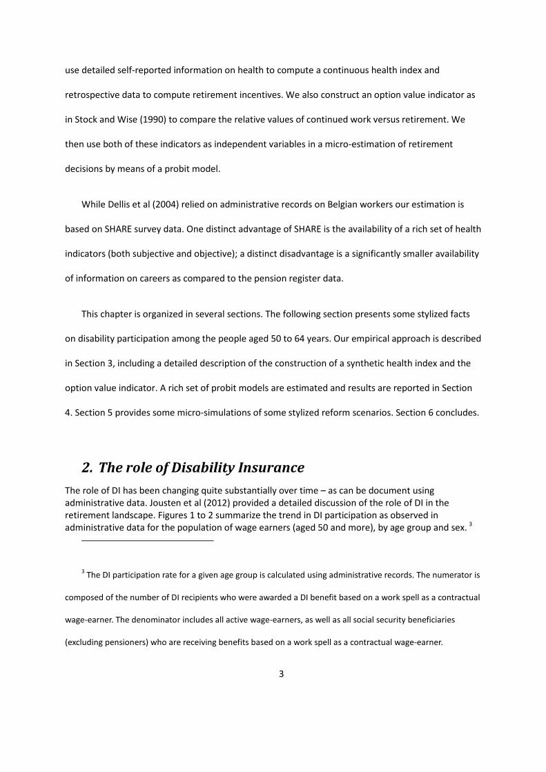
2. The role of Disability Insurance The role of DI has been changing quite substantially over time – as can be document using administrative data. Jousten et al (2012) provided a detailed discussion of the role of DI in the retirement landscape. Figures 1 to 2 summarize the trend in DI participation as observed in administrative data for the population of wage earners (aged 50 and more), by age group and sex. 3
3 The DI participation rate for a given age group is calculated using administrative records. The numerator is
composed of the number of DI recipients who were awarded a DI benefit based on a work spell as a contractual
wage-earner. The denominator includes all active wage-earners, as well as all social security beneficiaries
(excluding pensioners) who are receiving benefits based on a work spell as a contractual wage-earner.
4
Figure 1: DI participation rate, 1980-2010, Men age 50-64
Source: INAMI-RIZIV administrative records. Note: DI participation rates are obtained as percentage of beneficiaries as a share of the eligible wage-earner population in the age cohort.
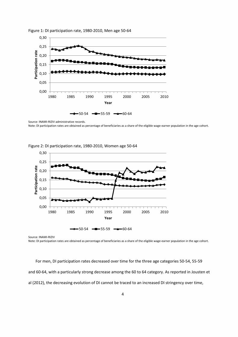
Figure 2: DI participation rate, 1980-2010, Women age 50-64
Source: INAMI-RIZIV Note: DI participation rates are obtained as percentage of beneficiaries as a share of the eligible wage-earner population in the age cohort.
For men, DI participation rates decreased over time for the three age categories 50-54, 55-59
and 60-64, with a particularly strong decrease among the 60 to 64 category. As reported in Jousten et
al (2012), the decreasing evolution of DI cannot be traced to an increased DI stringency over time,
0,00
0,05
0,10
0,15
0,20
0,25
0,30
1980 1985 1990 1995 2000 2005 2010
Part
icip
atio
n ra
te
Year
50-54 55-59 60-64
0,00
0,05
0,10
0,15
0,20
0,25
0,30
1980 1985 1990 1995 2000 2005 2010
Part
icip
atio
n ra
te
Year
50-54 55-59 60-64
5
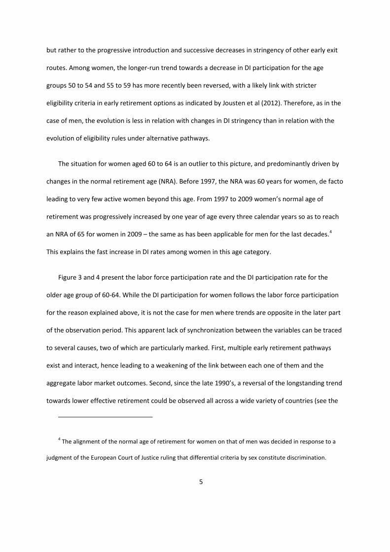
but rather to the progressive introduction and successive decreases in stringency of other early exit
routes. Among women, the longer-run trend towards a decrease in DI participation for the age
groups 50 to 54 and 55 to 59 has more recently been reversed, with a likely link with stricter
eligibility criteria in early retirement options as indicated by Jousten et al (2012). Therefore, as in the
case of men, the evolution is less in relation with changes in DI stringency than in relation with the
evolution of eligibility rules under alternative pathways.
The situation for women aged 60 to 64 is an outlier to this picture, and predominantly driven by
changes in the normal retirement age (NRA). Before 1997, the NRA was 60 years for women, de facto
leading to very few active women beyond this age. From 1997 to 2009 women’s normal age of
retirement was progressively increased by one year of age every three calendar years so as to reach
an NRA of 65 for women in 2009 – the same as has been applicable for men for the last decades.4
This explains the fast increase in DI rates among women in this age category.
Figure 3 and 4 present the labor force participation rate and the DI participation rate for the
older age group of 60-64. While the DI participation for women follows the labor force participation
for the reason explained above, it is not the case for men where trends are opposite in the later part
of the observation period. This apparent lack of synchronization between the variables can be traced
to several causes, two of which are particularly marked. First, multiple early retirement pathways
exist and interact, hence leading to a weakening of the link between each one of them and the
aggregate labor market outcomes. Second, since the late 1990’s, a reversal of the longstanding trend
towards lower effective retirement could be observed all across a wide variety of countries (see the
4 The alignment of the normal age of retirement for women on that of men was decided in response to a
judgment of the European Court of Justice ruling that differential criteria by sex constitute discrimination.

6
previous volumes of this series), and this to a large degree irrespectively of the incentive structure
prevailing in any specific country.
Figure 3: DI participation and labor force participation, 1980-2010, Men age 60-64
Source: INAMI-RIZIV, Eurostat Note: DI participation rates are obtained as percentage of beneficiaries as a share of the eligible wage-earner population in the age cohort.
Figure 4: DI participation and labor force participation, 1980-2010, Women age 60-64
Source: INAMI-RIZIV, Eurostat Note: DI participation rates are obtained as percentage of eligible wage-earner population in the same age cohort.
0,00
0,05
0,10
0,15
0,20
0,25
0,30
0,35
0,00
0,05
0,10
0,15
0,20
0,25
0,30
1980
1982
1984
1986
1988
1990
1992
1994
1996
1998
2000
2002
2004
2006
2008
2010
LFPR
DI p
artic
ipat
ion
rate
DI participation LFPR
0,00
0,02
0,04
0,06
0,08
0,10
0,12
0,14
0,16
0,00
0,05
0,10
0,15
0,20
0,25
1980
1982
1984
1986
1988
1990
1992
1994
1996
1998
2000
2002
2004
2006
2008
2010
LFPR
DI p
artic
ipat
ion
rate
DI participation LFPR

7
DI has a very diverse impact the various subgroups of the population – particularly when
comparing along the education and health dimensions. As Belgium does not have any systematically
collected administrative data on those topics, we turn to SHARE to derive some stylized facts. Figures
5 and 6 illustrate the evolution over the period ranging from the first wave of SHARE (2004-2005) to
the last one available to date (2010-2011). 5 They summarize the DI probabilities for male and female
wage-earners respectively, within the 50 to 64 age group stratified by education level. Overall, there
is a strong negative gradient between education level and DI probability for wage-earners. The sole
exception is the case of women in 2006/07 (SHARE wave 2), where the DI probability is higher for the
intermediate category than for the low educated, likely due to a small-sample problem.
Figure 5: DI probability by education, male wage earners age 50 to 64
Source: Authors’ calculation based on SHARE data (waves 1, 2 and 4). Note: DI probability is obtained as the number of individuals receiving DI benefits in the wage-earner population (active or unemployed).
5 Three waves of SHARE are useable for this analysis: waves 1 (2004-2005), 2 (2006-2007) and 4 (2010-
2011). Wave 3 conducted in 2008-2009 (known as SHARELIFE) does not include questions on individuals’
current situation, but mainly retrospective questions.
0,00
0,05
0,10
0,15
0,20
0,25
0,30
2004/05 2006/07 2010/11
Primary Secondary Tertiary

8
Figure 6: DI probability by education, female wage earners age 50 to 64
Source: Authors’ calculation based on SHARE data (waves 1, 2 and 4). Note: DI probability is obtained as the number of individuals receiving DI benefits in the wage-earner population (active or unemployed).
Figures 7 and 8 illustrate the evolution of DI probabilities among men and women, respectively,
by health quintiles. Without entering in the details of health quintiles computations, which will be
presented in detail in Section 4.3, we observe in these figures that DI probabilities are positively
related to health in SHARE, but above all that for people in the lower health quintile the DI
probability reaches values as high as 50% in some survey waves.
Figure 7: DI probability by health quintiles, male wage earners age 50 to 64
Source: Authors’ calculation based on SHARE data (waves 1, 2 and 4). Note: DI probability is obtained as the number of individuals receiving DI benefits in the total population.
0,00
0,05
0,10
0,15
0,20
0,25
0,30
2004/05 2006/07 2010/11
Primary Secondary Tertiary
0,00
0,10
0,20
0,30
0,40
0,50
0,60
2004/05 2006/07 2010/11
Quint1 (lowest) Quint2 Quint3 Quint4 Quint5 (highest)
9
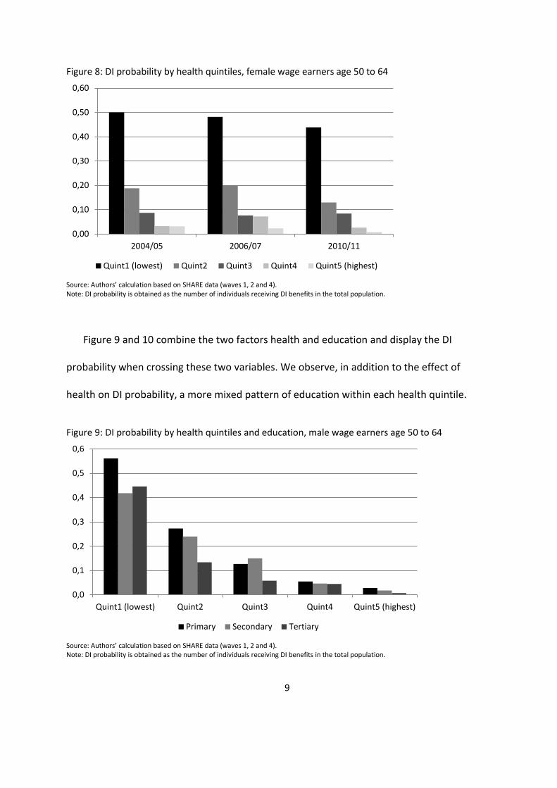
Figure 8: DI probability by health quintiles, female wage earners age 50 to 64
Source: Authors’ calculation based on SHARE data (waves 1, 2 and 4). Note: DI probability is obtained as the number of individuals receiving DI benefits in the total population.
Figure 9 and 10 combine the two factors health and education and display the DI
probability when crossing these two variables. We observe, in addition to the effect of
health on DI probability, a more mixed pattern of education within each health quintile.
Figure 9: DI probability by health quintiles and education, male wage earners age 50 to 64
Source: Authors’ calculation based on SHARE data (waves 1, 2 and 4). Note: DI probability is obtained as the number of individuals receiving DI benefits in the total population.
0,00
0,10
0,20
0,30
0,40
0,50
0,60
2004/05 2006/07 2010/11
Quint1 (lowest) Quint2 Quint3 Quint4 Quint5 (highest)
0,0
0,1
0,2
0,3
0,4
0,5
0,6
Quint1 (lowest) Quint2 Quint3 Quint4 Quint5 (highest)
Primary Secondary Tertiary
10
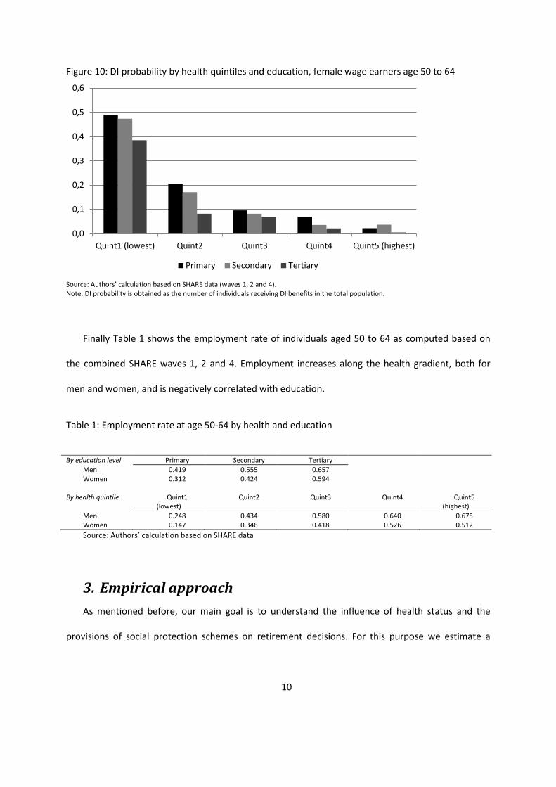
Figure 10: DI probability by health quintiles and education, female wage earners age 50 to 64
Source: Authors’ calculation based on SHARE data (waves 1, 2 and 4). Note: DI probability is obtained as the number of individuals receiving DI benefits in the total population.
Finally Table 1 shows the employment rate of individuals aged 50 to 64 as computed based on
the combined SHARE waves 1, 2 and 4. Employment increases along the health gradient, both for
men and women, and is negatively correlated with education.
Table 1: Employment rate at age 50-64 by health and education
By education level Primary Secondary Tertiary Men 0.419 0.555 0.657 Women 0.312 0.424 0.594
By health quintile Quint1 (lowest)
Quint2
Quint3
Quint4
Quint5 (highest)
Men 0.248 0.434 0.580 0.640 0.675 Women 0.147 0.346 0.418 0.526 0.512 Source: Authors’ calculation based on SHARE data
3. Empirical approach As mentioned before, our main goal is to understand the influence of health status and the
provisions of social protection schemes on retirement decisions. For this purpose we estimate a
0,0
0,1
0,2
0,3
0,4
0,5
0,6
Quint1 (lowest) Quint2 Quint3 Quint4 Quint5 (highest)
Primary Secondary Tertiary

11
discrete-time retirement model in which exit from the labor market ( )1=iR is explained by social
protection incentives, health and other covariates.
For individual i:
[ ] [ ]iiii HOVXR γδβ ++== 'Pr1Pr (1)
where 'iX is a vector of taste-shifters variables, iOV is a social security incentive, an option value
measure, and iH is a measure of health status.
In our econometric analysis, we use the first two waves of data from SHARE collected in 2004-05
and 2006-07 for Belgium. The third wave of data, known as SHARELIFE (collected in 2008-09), asked
all previous respondents (waves 1 and 2) and their partners to provide information not on their
current situation but on their entire life–histories. This provides retrospective information on
childhood, health, living and professional career. We combine the first two waves with the
retrospective data from SHARELIFE to obtain a full career history for each individual.6 For individuals
surveyed in any wave we can observe when they exited the labor market and through which
pathways. This means that while there are usually 2 years between each wave we can observe a
year-to-year transitions. The advantage is that instead of seeing an individual just once between two
waves, we follow him along the years between two waves and we know his actual status in each
year. We restrict the sample to the individuals who are aged between 50 and 64. In each wave (1 or
2) we select those individuals who were employed as wage earners and exclude retired, unemployed,
sick and disabled. We also exclude individuals for whom retrospective information is not available in
6 SHARE wave 4 data was also available but not usable for this purpose given that wave 3, SHARELIFE, did
not report detailed information on health and on other key variables for this study.
12
SHARELIFE. Finally we drop all the records for the years that are subsequent to the year when the
individual exited the labor force. Our analytical sample consists of 1,210 observations.
Two crucial steps in our analysis relate to the derivation of a synthetic health measure and the
calculation of a summary indicator of retirement incentives. For the former, we rely on a continuous
health index computed using a principle component analysis based on nearly 25 self-reported health
indicators. For the latter, we rely on an “inclusive” version of the concept of option value, de facto a
weighted average of the option values for each pathway to retirement. We detail the approach
below.
3.1. Measurement of health status Identifying the effects of health on retirement is complicated because people’s health is not
directly observable. The use of surveys wherein people report subjective self-assessments of their
physical capacity can often be misleading. Indeed, it is a subjective assessment and there is no reason
to expect that such assessments are entirely comparable across individuals. Also, answers may not
be independent of the outcomes we wish to study. For example, individuals who are inactive often
have an incentive to report worse than actual health. In such situations, subjective health indicators
measure leisure preferences rather than true health status.
It is thus preferable to use objective indicators of health. The issue is to find objective measures
that are correlated with work capacity and that truly reflect the individuals’ ability to work. The
SHARE data contain a variety of objective and subjective measures of health. Using objective
measures of physical ability in addition to self-reported health status, we propose to derive a latent
health index similar to Poterba et al (2010). To construct the index we use responses to 24 questions
and obtain the first principal component of these underlying indicators of health. The first principal
component is the weighted average of the health indicators, where the weights are chosen to

13
maximize the proportion of the variance of the indicators that can be explained by the first principal
component.7
All data from waves 1, 2 and 4 of SHARE are used to calculate the principal components. These
are then in a second step applied to all observations of waves 1 and 2 that are the basis for our
econometric analysis – de facto attributing a health index for each individual in each one of the two
waves under study. Thus an individual may experience changes of the health status across the survey
waves. The health score obtained from the first principal component is converted into percentile
scores for each observation with 1 the worst health and 100 the best. Later on the analysis we group
persons by health status quintiles using this score. Figure 11 displays the average health percentile in
Belgium by age. We observe in this figure that, as expected, the health indicator decreases with age,
with a blip at age 60.
7 The list of health questions used in the principal component analysis is available in the Appendix, as well
as the correlation coefficients corresponding to the first component.

14
Figure 11: Average health percentile by age
Source: Authors calculation based on SHARE data waves 1 and 2
3.2. Pathways to retirement Wage earners face several typical pathways to retirement. A first pathway consists of an
immediate transfer from work into the old age pension system (OAP). The OAP currently allows
claiming early retirement as of age 60, when some career requirements are met. The normal
retirement age, at which anybody can claim OAP benefit independently of career requirements, is
currently set at age 65 for both men and women. Notice that during the first two waves of SHARE
data collection from 2004-2005, the normal retirement age for women was still under the transitory
regime reaching 63 for the first wave and 64 for the second.
Benefits correspond to 75% of average lifetime earnings for one-earner couples and to 60% for
singles – with two earner couples having the right to a top-up to the said 75 percent if the secondary
earner’s pension is smaller than this household supplement. Claiming early does not imply any
actuarial adjustment of benefits as compared to claiming at NRA.
A full career corresponds to 45 years of earnings or assimilated periods, with average lifetime
earnings computed over the same 45 year period. A specificity of the Belgian retirement landscape is
0
10
20
30
40
50
60
70
50 51 52 53 54 55 56 57 58 59 60 61 62 63 64 65
15
that periods spent on replacement income (such as CER, UI or DI) fully count as years worked in the
computation of the retirement benefits. For any such periods, fictive wages are inserted into the
earnings history. For the period of our analysis, these fictive wages correspond to the real wage that
the individual was earning right before his period of inactivity. Benefits are shielded against inflation
through an automatic price adjustment and an earning test frequently applies before the NRA.
Next to the public pension system, several early retirement pathways have emerged. The CER
program was explicitly designed as an early exit route. It is based on collective agreements, which are
negotiated between employee and employer associations. Within this program, the workers exit the
labor market and receive an unemployment compensation paid by the UI system and a bonus paid
by the employer, which equals half of the difference between the individual’s last net wage and the
special unemployment benefit applicable to CER beneficiaries. Both benefits and reference wage
have caps and floors. The CER program implies that workers cannot draw public pension benefits
before the NRA, at which age he is automatically rolled over into the OAP system. The generally
applicable eligibility rule sets out that they have to satisfy a minimum age of 58 and a career of at
least 25 years, but exceptions exist that allow some workers to exit through CER as early as age 50
with as little as a career of 10 years.
Regular UI benefits represent a second effective exit route into retirement. In Belgium there is no
generally applicable time limit for UI benefit receipt, except for the automatic rollover provision of
unemployed into retirement upon reaching the NRA. The level of these benefits depends on the
family status and the duration of the unemployment spell. In theory, they are equal to 60% of the
previous net wage if the individual is single or has family dependents. If the spouse or partner has
income, benefits are equal to 55% of last net wage. In practice, they have caps and floors that vary
according to the duration of the unemployment spell, de facto somewhat weakening the mechanical
nature of the mentioned replacement rates.

16
Within the group of unemployed, special rules are applicable to some categories of older
workers, a system known as Old-Age Unemployment (OAU) as documented in Jousten et al (2012).
While the system has played an important role in the Belgian retirement landscape, we do not
explicitly take it into account in our analysis for two reasons. First, in SHARE data, OAU is
observationally indistinguishable from UI. Second, successive policy changes over the course of the
last decade have effectively dismantled the system as a stand-alone program and brought it back into
the realm of the regular UI. In fact, the two key benefits of the system as compared to regular UI
have been decoupled and significantly tightened: a waiver from the general job search requirement
and the conditions for benefiting from a seniority supplement.
Last but not least, though a priori exclusively targeted at those withdrawing from the labor
market for reasons of bad health, DI may also serve as an early exit route. The eligibility is based on
loss of earnings capacity. In order to be eligible, the worker has to suffer from a loss of earnings
capacity of 66% over a period of 12 months. The benefit level is a function of the household status
and is equal to 65% of reference wage if the worker has dependents. It is reduced to 53% if the
insured lives alone and to 45% if the individual cohabits. As for unemployment, benefits are payable
up to the NRA with automatic rollover into OAP occurring at that age.
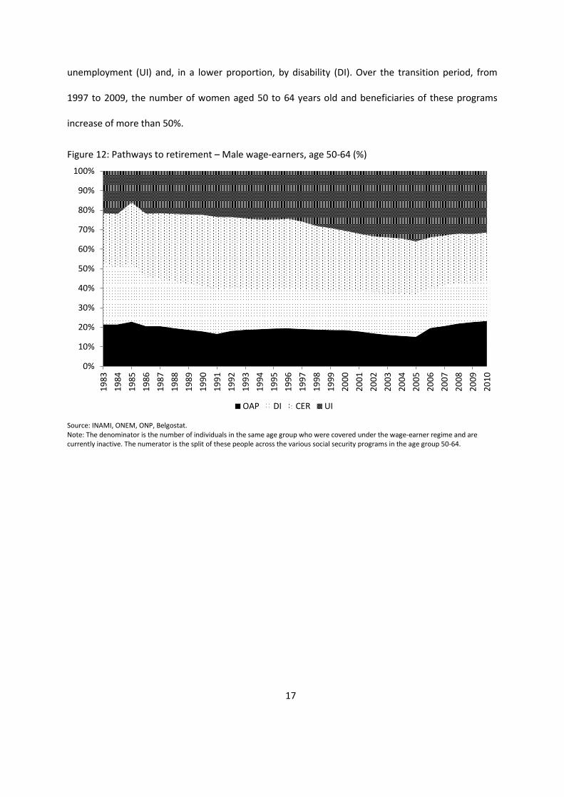
Figures 12 and 13 provide empirical evidence on the importance of the various programs across
time, for men and women separately. The percentages are computed as the proportion of all social
protection beneficiaries, within the 50 to 64 years old category, in a particular program at each year.
We see the role of the various pathways in absorbing the change in one or another – with UI
effectively playing the role of program of last resort.
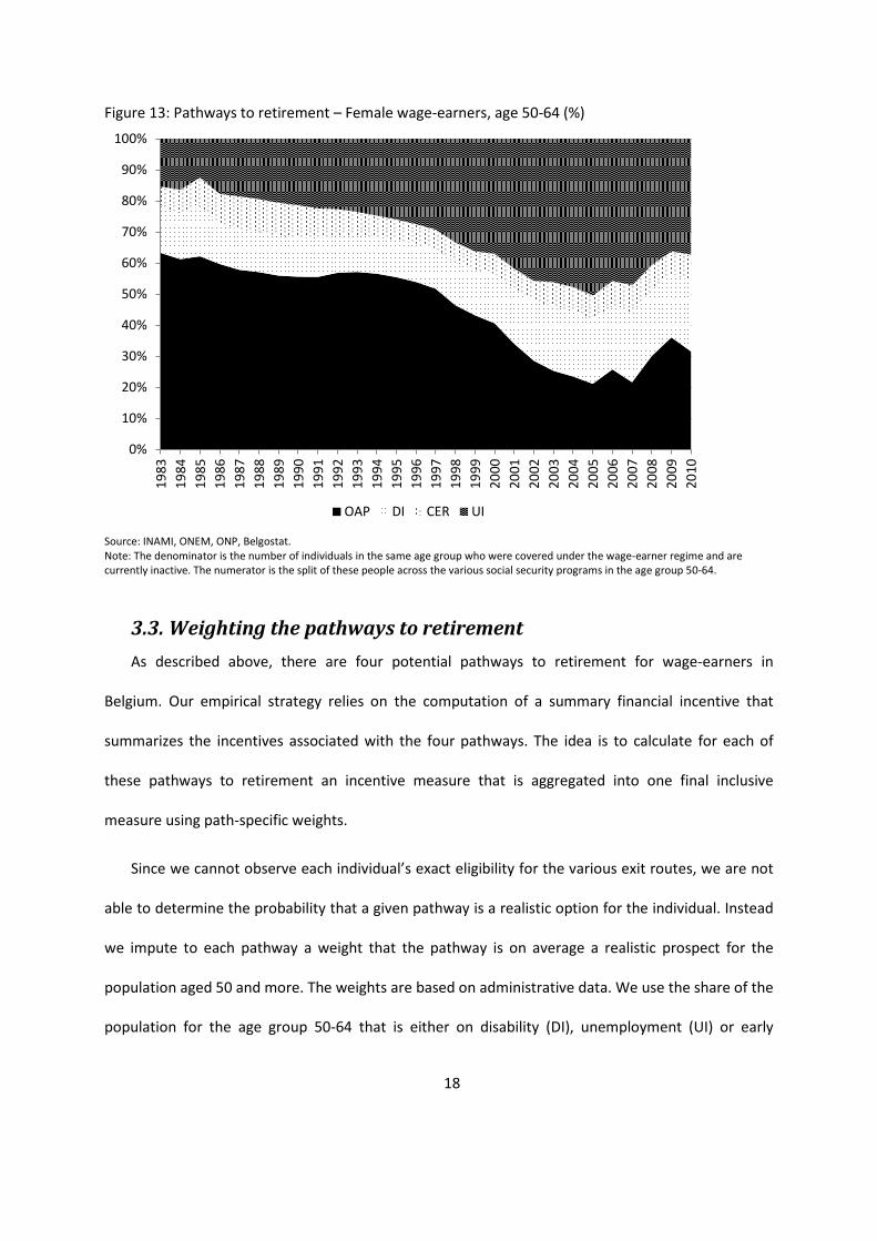
For men we observe over the last years an increase in the proportion of pensioners (OAP). For
women, Figure 13, we observe on the contrary a dramatic decrease in the proportion of pensioners,
due to the progressive postponement of the NRA from 60 to 65 compensated mainly by
17
unemployment (UI) and, in a lower proportion, by disability (DI). Over the transition period, from
1997 to 2009, the number of women aged 50 to 64 years old and beneficiaries of these programs
increase of more than 50%.
Figure 12: Pathways to retirement – Male wage-earners, age 50-64 (%)
Source: INAMI, ONEM, ONP, Belgostat. Note: The denominator is the number of individuals in the same age group who were covered under the wage-earner regime and are currently inactive. The numerator is the split of these people across the various social security programs in the age group 50-64.
0%
10%
20%
30%
40%
50%
60%
70%
80%
90%
100%
1983
1984
1985
1986
1987
1988
1989
1990
1991
1992
1993
1994
1995
1996
1997
1998
1999
2000
2001
2002
2003
2004
2005
2006
2007
2008
2009
2010
OAP DI CER UI
18
Figure 13: Pathways to retirement – Female wage-earners, age 50-64 (%)
Source: INAMI, ONEM, ONP, Belgostat. Note: The denominator is the number of individuals in the same age group who were covered under the wage-earner regime and are currently inactive. The numerator is the split of these people across the various social security programs in the age group 50-64.
3.3. Weighting the pathways to retirement As described above, there are four potential pathways to retirement for wage-earners in
Belgium. Our empirical strategy relies on the computation of a summary financial incentive that
summarizes the incentives associated with the four pathways. The idea is to calculate for each of
these pathways to retirement an incentive measure that is aggregated into one final inclusive
measure using path-specific weights.
Since we cannot observe each individual’s exact eligibility for the various exit routes, we are not
able to determine the probability that a given pathway is a realistic option for the individual. Instead
we impute to each pathway a weight that the pathway is on average a realistic prospect for the
population aged 50 and more. The weights are based on administrative data. We use the share of the
population for the age group 50-64 that is either on disability (DI), unemployment (UI) or early
0%
10%
20%
30%
40%
50%
60%
70%
80%
90%
100%19
8319
8419
8519
8619
8719
8819
8919
9019
9119
9219
9319
9419
9519
9619
9719
9819
9920
0020
0120
0220
0320
0420
0520
0620
0720
0820
0920
10
OAP DI CER UI

19
retirement (CER). Old age pension (OAP) takes the residual such that the sum of the weights is equal
to one. The 50-64 age-window corresponds to the main ages at-risk of retirement in Belgium. Figures
14 and 15 present these weights for the last twenty years. Interestingly, we observe for men a
decrease of the weight of disability but an increase for women due to the postponement of women’
normal age of retirement.
Figure 14: Pathway weights by year – Male wage-earners, age 50-64
Source: INAMI, ONEM, Belgostat
Figure 15: Pathway weights by year – Male wage-earners, age 50-64
Source: INAMI, ONEM, Belgostat
0,00,10,20,30,40,50,60,70,80,91,0
1987
1988
1989
1990
1991
1992
1993
1994
1995
1996
1997
1998
1999
2000
2001
2002
2003
2004
2005
2006
2007
2008
2009
2010
OAP CER UI DI
0,00,10,20,30,40,50,60,70,80,91,0
1987
1988
1989
1990
1991
1992
1993
1994
1995
1996
1997
1998
1999
2000
2001
2002
2003
2004
2005
2006
2007
2008
2009
2010
OAP CER UI DI

20
3.4. Option value calculations Thanks to the data from SHARELIFE we are able to reconstruct the individual’s career history and
thus ultimately to calculate the entitlements to benefits. SHARELIFE asks the respondents to provide
start and end dates of each paid job they had, the characteristics of the job, as well as the first
monthly wage. For those who are still employed at the time of the interview, the last monthly wage
is also asked. All these amounts are after taxes.
This information is used to construct a panel with one wage observation per year for each
individual, from the first job until the interview year. For simplicity we convert all amounts to EUR of
2008. The wage path is obtained using linear interpolation of wages for the years where we lack
wage information. During unemployment, sickness and disability as well as early retirement periods,
fictive wages equal to the last observed wage are assigned, as required by calculation rules of public
pension. As a result, we can project each individual’s entitlements under the 4 exit routes based on
each individual’s own earnings history.
As indicated before, our financial incentive measure (OV) is a forward-looking measure based on
the concept of option value of retirement, as defined by Stock and Wise (1990). In the option value
model, an individual evaluates the expected present discounted value of income for all possible
future retirement ages through a route to retirement and then compares the value of retirement
today versus the value at the optimal age. It is based on a utility-maximization framework. Under the
reduced form formulation, the value at age a of retirement h, )(hVa , is given by (to simplify the
presentation, we hide here the individual’s subscript index i):
[ ]∑∑=
−−
=
− +=s
as
γh
asγs
h
as
asa skBρsθWρsθhV )()()()(
1
(2)

21
Where )(sθ is the survival probability at age s, ρ is the rate of time preference and )(sBh is the
benefit expected at age s if the worker retires at age h. sW is the earnings from continued working.
Depending on the household situation, )(sθ also accounts for survivor benefits.8
The variable γ is a parameter of relative risk aversion and is set equal to 0.75. Finally, the
parameter k expresses the relative weight of utility of retirement income and is set equal to 1.5.
Letting *h be the year in the future at which the individual maximizes her/his expected value of
retiring, the option value (OV) is then defined as the difference in utility terms between retiring at
the best point in the future ( )*h or now ( )a :
)()()( ** aVhVhOV aaa −= (3)
We rely on an inclusive version of the option value that is a weighted average of the option value
associated to each potential route (pathway) to retirement. In order to compute the OV for each
pathway to retirement, we need to make a projection of individual-level wages. In our analysis, we
assume a real growth of wages of 0 going forward. Using this information and the whole career
information compiled from SHARELIFE, we compute expected benefit flows for every pathway to
retirement (DI, UI, CER and OAP) for each possible age of retirement up to the NRA. Finally, we
integrate expected benefits and expected wages in equations (2) and (3) to derive the option value
for each retirement pathway.
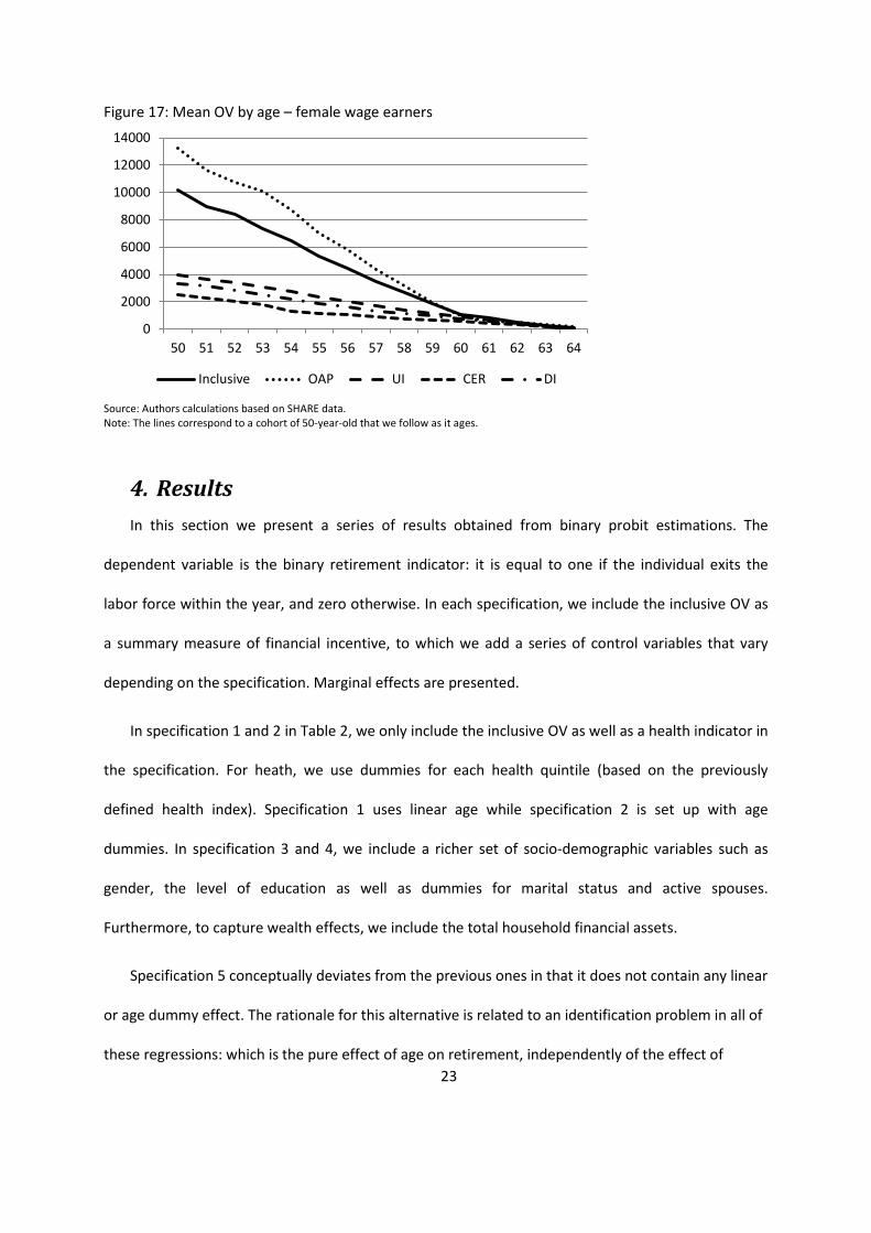
Figure 16 and 17 show the mean OV for each pathway for men and women. The pattern is
downward sloping for each OV as well as for both men and women. That is that the utility to be
8 We use a discount rate of 3% which is very often used in the literature. Mortality tables by sex for the
Belgian population are used to compute θ(s). The source is the Human Mortality Database (www.mortality.org).
22
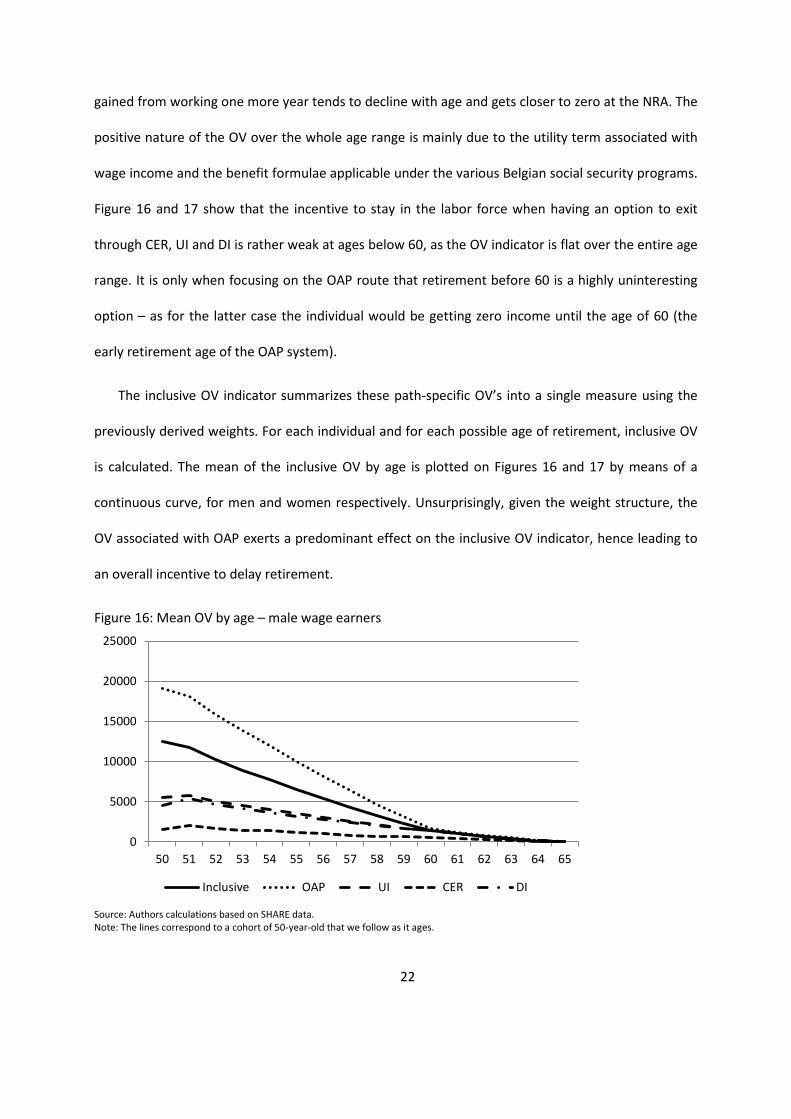
gained from working one more year tends to decline with age and gets closer to zero at the NRA. The
positive nature of the OV over the whole age range is mainly due to the utility term associated with
wage income and the benefit formulae applicable under the various Belgian social security programs.
Figure 16 and 17 show that the incentive to stay in the labor force when having an option to exit
through CER, UI and DI is rather weak at ages below 60, as the OV indicator is flat over the entire age
range. It is only when focusing on the OAP route that retirement before 60 is a highly uninteresting
option – as for the latter case the individual would be getting zero income until the age of 60 (the
early retirement age of the OAP system).
The inclusive OV indicator summarizes these path-specific OV’s into a single measure using the
previously derived weights. For each individual and for each possible age of retirement, inclusive OV
is calculated. The mean of the inclusive OV by age is plotted on Figures 16 and 17 by means of a
continuous curve, for men and women respectively. Unsurprisingly, given the weight structure, the
OV associated with OAP exerts a predominant effect on the inclusive OV indicator, hence leading to
an overall incentive to delay retirement.
Figure 16: Mean OV by age – male wage earners
Source: Authors calculations based on SHARE data. Note: The lines correspond to a cohort of 50-year-old that we follow as it ages.
0
5000
10000
15000
20000
25000
50 51 52 53 54 55 56 57 58 59 60 61 62 63 64 65
Inclusive OAP UI CER DI
23
Figure 17: Mean OV by age – female wage earners
Source: Authors calculations based on SHARE data. Note: The lines correspond to a cohort of 50-year-old that we follow as it ages.
4. Results In this section we present a series of results obtained from binary probit estimations. The
dependent variable is the binary retirement indicator: it is equal to one if the individual exits the
labor force within the year, and zero otherwise. In each specification, we include the inclusive OV as
a summary measure of financial incentive, to which we add a series of control variables that vary
depending on the specification. Marginal effects are presented.
In specification 1 and 2 in Table 2, we only include the inclusive OV as well as a health indicator in
the specification. For heath, we use dummies for each health quintile (based on the previously
defined health index). Specification 1 uses linear age while specification 2 is set up with age
dummies. In specification 3 and 4, we include a richer set of socio-demographic variables such as
gender, the level of education as well as dummies for marital status and active spouses.
Furthermore, to capture wealth effects, we include the total household financial assets.
Specification 5 conceptually deviates from the previous ones in that it does not contain any linear
or age dummy effect. The rationale for this alternative is related to an identification problem in all of
these regressions: which is the pure effect of age on retirement, independently of the effect of
0
2000
4000
6000
8000
10000
12000
14000
50 51 52 53 54 55 56 57 58 59 60 61 62 63 64
Inclusive OAP UI CER DI
24
pension schemes rules? The data we use does not allow us to address this identification issue, many
more waves of SHARE would be necessary. Hence, in specifications 1 to 4, the age dummies or the
linear age trend capture a mix of both.
In specification 5 we take an extreme alternative by estimating the effect of OV under the
assumption that any age-of-eligibility effect is fully taken into account by the inclusive OV variable.
Implicitly, this also implies that we give the inclusive OV incentive variable a maximum role, though it
does not by itself address the identification problem – it just takes a slightly different view. The
approach turns out to be particularly useful when trying to gauge the effect of reform simulations
(see the next section).
Finally, Specifications 6 to 10 are similar to the five first specifications except that it includes a
different indicator for the health status of individuals. In this second batch of specifications, health is
introduced as the linear health index obtained from the principal component analysis rather than the
relative position in the population by quintile.
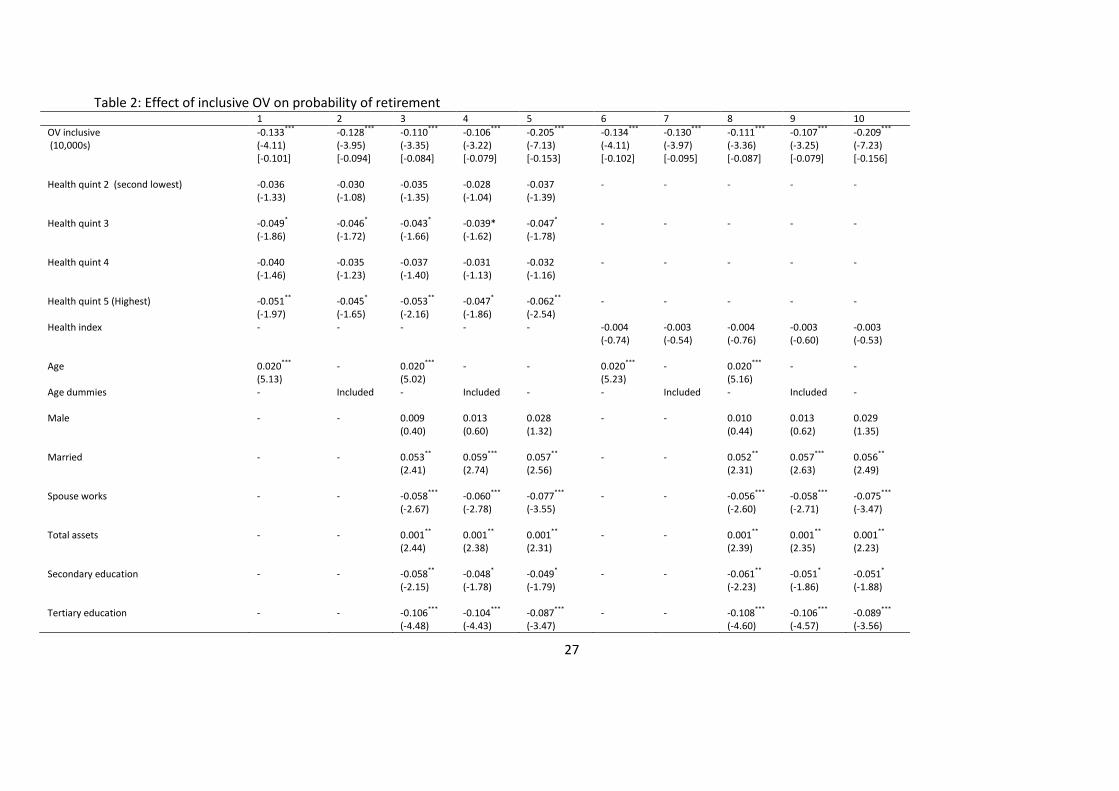
The incentive measure turns out to be strongly significant in all specifications. The effect is
negative, as expected, which means that a larger value of continued work leads to lower probability
of retirement. In brackets, we also report the effect of a one-standard-deviation change in the OV as
the coefficient on the OV can be sensitive to the mean and the variance of the OV. The results are
similar to those for the coefficient on OV. In line with expectations, specifications 5 and 10 show a
much bigger effect of the inclusive OV as it now captures the full scope of incentives that are
otherwise partially captured by the age term.
Regarding health, results are somewhat unexpected. Individuals in the fifth quintile are
significantly less likely to retire (at thresholds of 5 or 10 percent, according to the specification) than
individuals in the first quintile. Only for some specifications and for a 10 percent significance level,
25
individuals of the third quintile also display similar features. When looking at specifications with the
health index, no significant pattern can be distinguished as a function of the health index. This even
holds true when interacting the incentive measure with the health index as in Table 3.
Our findings with regards to the influence of health status have clear policy relevance: our
findings show that the link between health and retirement in Belgium is either weak or not
significant. This stands in sharp contrast to the analysis of section 2, indicating the importance of
performing econometric analysis instead of relying on mere correlations.
While the gender dummy is insignificant, other variables have strong impacts: Age plays a
significant role. Education also has a strong explanatory power, with higher education leading to
significantly lower retirement probabilities. Being married has a positive impact on the likelihood of
retirement, while having an active spouse reduces the retirement probability. Household financial
wealth also leads to a higher probability of retirement – in line with intuition.
Table 4 is analogous to specification 1 to 4 of Table 2 but instead of the inclusive OV, we use the
percent gain in the utility from delaying retirement till the optimal retirement date. The underlying
idea is simple: a similar level of OV can represent very different realities for different individuals, as
they may have very different starting positions in terms of initial incomes and well-being. Hence, we
define this percent gain in the utility of delayed retirement as the ratio of OV to the level of utility the
individual would obtain if he were to immediately retire.9
The estimated coefficients on the incentive variable again turn out highly significant and robust
to the specification choice. The observed effect of the financial incentive variable is much stronger
9 In terms of the terminology of the previous section, this corresponds to dividing expression (3) by
expression (2), the latter evaluated upon immediate retirement.

26
than in Table 2, indicating that the relation to initial levels of well-being matter in the Belgian
retirement landscape.10
10 We have tested alternative specifications including the two terms of this ratio as separate variables and
have not found any stable relation. Results can be obtained from the authors upon request.
27
Table 2: Effect of inclusive OV on probability of retirement 1 2 3 4 5 6 7 8 9 10 OV inclusive -0.133*** -0.128*** -0.110*** -0.106*** -0.205*** -0.134*** -0.130*** -0.111*** -0.107*** -0.209*** (10,000s) (-4.11) (-3.95) (-3.35) (-3.22) (-7.13) (-4.11) (-3.97) (-3.36) (-3.25) (-7.23) [-0.101] [-0.094] [-0.084] [-0.079] [-0.153] [-0.102] [-0.095] [-0.087] [-0.079] [-0.156] Health quint 2 (second lowest) -0.036 -0.030 -0.035 -0.028 -0.037 - - - - - (-1.33) (-1.08) (-1.35) (-1.04) (-1.39) Health quint 3 -0.049* -0.046* -0.043* -0.039* -0.047* - - - - - (-1.86) (-1.72) (-1.66) (-1.62) (-1.78) Health quint 4 -0.040 -0.035 -0.037 -0.031 -0.032 - - - - - (-1.46) (-1.23) (-1.40) (-1.13) (-1.16) Health quint 5 (Highest) -0.051** -0.045* -0.053** -0.047* -0.062** - - - - - (-1.97) (-1.65) (-2.16) (-1.86) (-2.54) Health index - - - - - -0.004 -0.003 -0.004 -0.003 -0.003 (-0.74) (-0.54) (-0.76) (-0.60) (-0.53) Age 0.020*** - 0.020*** - - 0.020*** - 0.020*** - - (5.13) (5.02) (5.23) (5.16) Age dummies - Included - Included - - Included - Included - Male - - 0.009 0.013 0.028 - - 0.010 0.013 0.029 (0.40) (0.60) (1.32) (0.44) (0.62) (1.35) Married - - 0.053** 0.059*** 0.057** - - 0.052** 0.057*** 0.056** (2.41) (2.74) (2.56) (2.31) (2.63) (2.49) Spouse works - - -0.058*** -0.060*** -0.077*** - - -0.056*** -0.058*** -0.075*** (-2.67) (-2.78) (-3.55) (-2.60) (-2.71) (-3.47) Total assets - - 0.001** 0.001** 0.001** - - 0.001** 0.001** 0.001** (2.44) (2.38) (2.31) (2.39) (2.35) (2.23) Secondary education - - -0.058** -0.048* -0.049* - - -0.061** -0.051* -0.051* (-2.15) (-1.78) (-1.79) (-2.23) (-1.86) (-1.88) Tertiary education - - -0.106*** -0.104*** -0.087*** - - -0.108*** -0.106*** -0.089*** (-4.48) (-4.43) (-3.47) (-4.60) (-4.57) (-3.56)
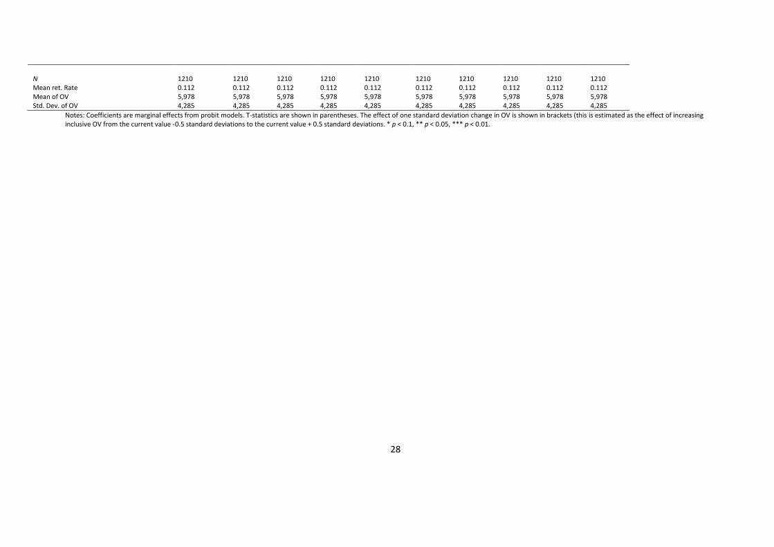
28
N 1210 1210 1210 1210 1210 1210 1210 1210 1210 1210 Mean ret. Rate 0.112 0.112 0.112 0.112 0.112 0.112 0.112 0.112 0.112 0.112 Mean of OV 5,978 5,978 5,978 5,978 5,978 5,978 5,978 5,978 5,978 5,978 Std. Dev. of OV 4,285 4,285 4,285 4,285 4,285 4,285 4,285 4,285 4,285 4,285
Notes: Coefficients are marginal effects from probit models. T-statistics are shown in parentheses. The effect of one standard deviation change in OV is shown in brackets (this is estimated as the effect of increasing inclusive OV from the current value -0.5 standard deviations to the current value + 0.5 standard deviations. * p < 0.1, ** p < 0.05, *** p < 0.01.
29
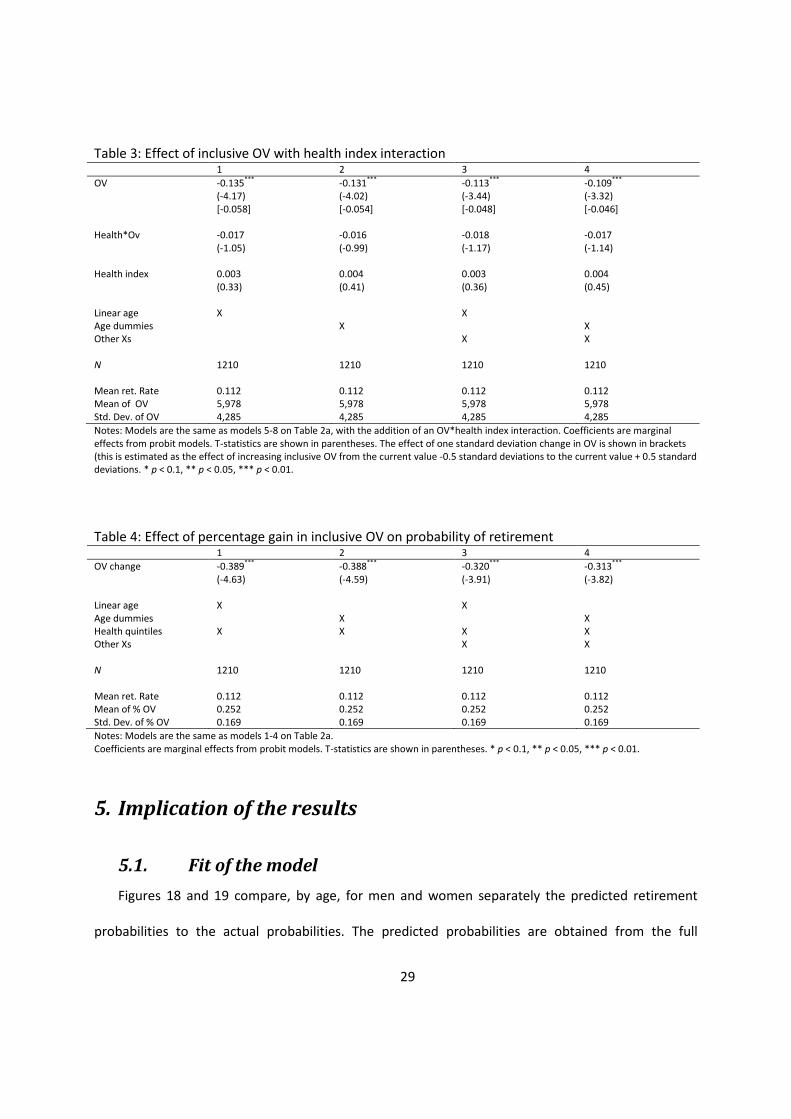
Table 3: Effect of inclusive OV with health index interaction 1 2 3 4 OV -0.135*** -0.131*** -0.113*** -0.109*** (-4.17) (-4.02) (-3.44) (-3.32) [-0.058] [-0.054] [-0.048] [-0.046] Health*Ov -0.017 -0.016 -0.018 -0.017 (-1.05) (-0.99) (-1.17) (-1.14) Health index 0.003 0.004 0.003 0.004 (0.33) (0.41) (0.36) (0.45) Linear age X X Age dummies X X Other Xs X X N 1210 1210 1210 1210 Mean ret. Rate 0.112 0.112 0.112 0.112 Mean of OV 5,978 5,978 5,978 5,978 Std. Dev. of OV 4,285 4,285 4,285 4,285 Notes: Models are the same as models 5-8 on Table 2a, with the addition of an OV*health index interaction. Coefficients are marginal effects from probit models. T-statistics are shown in parentheses. The effect of one standard deviation change in OV is shown in brackets (this is estimated as the effect of increasing inclusive OV from the current value -0.5 standard deviations to the current value + 0.5 standard deviations. * p < 0.1, ** p < 0.05, *** p < 0.01.
Table 4: Effect of percentage gain in inclusive OV on probability of retirement 1 2 3 4 OV change -0.389*** -0.388*** -0.320*** -0.313*** (-4.63) (-4.59) (-3.91) (-3.82) Linear age X X Age dummies X X Health quintiles X X X X Other Xs X X N 1210 1210 1210 1210 Mean ret. Rate 0.112 0.112 0.112 0.112 Mean of % OV 0.252 0.252 0.252 0.252 Std. Dev. of % OV 0.169 0.169 0.169 0.169 Notes: Models are the same as models 1-4 on Table 2a. Coefficients are marginal effects from probit models. T-statistics are shown in parentheses. * p < 0.1, ** p < 0.05, *** p < 0.01.
5. Implication of the results
5.1. Fit of the model Figures 18 and 19 compare, by age, for men and women separately the predicted retirement
probabilities to the actual probabilities. The predicted probabilities are obtained from the full

30
specification with health quintiles and age dummies (specification 4 in Table 2). It will be our baseline
for the simulations hereafter. The predictions follow closely the change in the actual probabilities,
both for men and women. Although not reported here, the predictions made on the basis of
estimations with a linear age are not so good. This indicates that the age dummies are important to
capture some of the nonlinearities that the incentives or the health cannot capture; such as the key
role played by eligibility ages.
Figure 18: Actual vs. predicted retirement probabilities, male wage earners
Source: Authors calculation based on SHARE data.
00,10,20,30,40,50,60,70,80,9
1
50 51 52 53 54 55 56 57 58 59 60 61 62 63 64
Actual Predicted
31
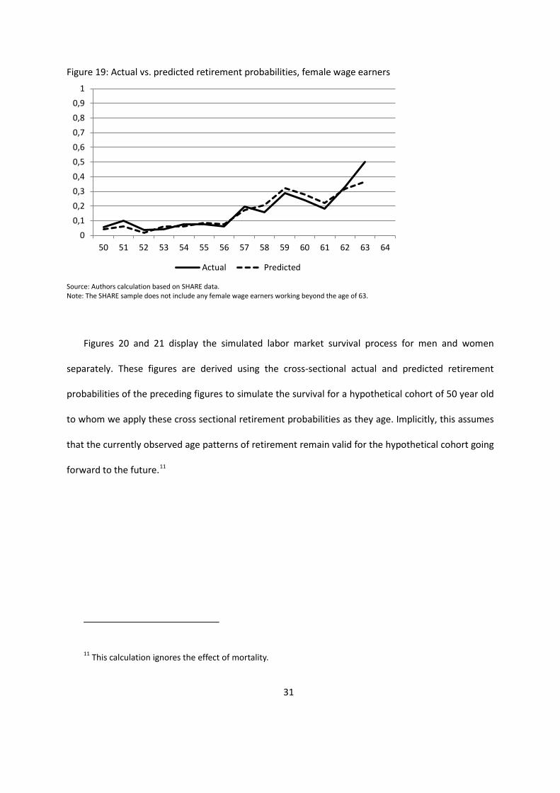
Figure 19: Actual vs. predicted retirement probabilities, female wage earners
Source: Authors calculation based on SHARE data. Note: The SHARE sample does not include any female wage earners working beyond the age of 63.
Figures 20 and 21 display the simulated labor market survival process for men and women
separately. These figures are derived using the cross-sectional actual and predicted retirement
probabilities of the preceding figures to simulate the survival for a hypothetical cohort of 50 year old
to whom we apply these cross sectional retirement probabilities as they age. Implicitly, this assumes
that the currently observed age patterns of retirement remain valid for the hypothetical cohort going
forward to the future.11
11 This calculation ignores the effect of mortality.
00,10,20,30,40,50,60,70,80,9
1
50 51 52 53 54 55 56 57 58 59 60 61 62 63 64
Actual Predicted
32
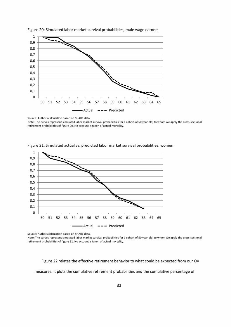
Figure 20: Simulated labor market survival probabilities, male wage earners
Source: Authors calculation based on SHARE data. Note: The curves represent simulated labor market survival probabilities for a cohort of 50 year old, to whom we apply the cross-sectional retirement probabilities of figure 20. No account is taken of actual mortality.
Figure 21: Simulated actual vs. predicted labor market survival probabilities, women
Source: Authors calculation based on SHARE data. Note: The curves represent simulated labor market survival probabilities for a cohort of 50 year old, to whom we apply the cross-sectional retirement probabilities of figure 21. No account is taken of actual mortality.
Figure 22 relates the effective retirement behavior to what could be expected from our OV
measures. It plots the cumulative retirement probabilities and the cumulative percentage of
00,10,20,30,40,50,60,70,80,9
1
50 51 52 53 54 55 56 57 58 59 60 61 62 63 64 65
Actual Predicted
00,10,20,30,40,50,60,70,80,9
1
50 51 52 53 54 55 56 57 58 59 60 61 62 63 64 65
Actual Predicted

33
individuals who, according to our incentive measures, have reached the maximum utility. It
shows that a large majority of wage-earners in Belgium retire before they have reached the
utility maximizing age of retirement as predicted by the model.
Figure 22: Share of wage-earners having reached maximum utility and cumulative retirement probability by age
Source: Authors calculation based on SHARE data.
5.2. Simulations Using our estimations results of Section 4 we investigate the effect of a change in the Belgian
retirement architecture on retirement behavior. We use specification 4 of Table 2 as our reference.
The first type of simulation (Simulation 1) considers that all persons in the sample face only one
of the four exit routes rather than a weighted combination of all. Expressed differently, we simulate
the impact on retirement behavior of restricting access – and thus OV’s – to one of the programs:
OAP, CER, UI or DI. We apply the estimated coefficients of the inclusive OV to these path-specific
OV’s. Implicitly, we thus view our estimates from the previous section as being instrumented
estimates of the true relations – with the population-wide averages serving as instruments for true
individual eligibility. Figure 23 summarizes the results in terms of retirement hazards by age under
0,0
0,2
0,4
0,6
0,8
1,0
50 51 52 53 54 55 56 57 58 59 60 61 62 63 64
% reached max utility, Men % reached max utility, Women
Exit rate, Men + Women

34
the alternative scenarios. In line with figures 16 and 17, the strongest differences appear between
the OAP and the other pathways with OAP leading to substantially lower hazard rates. Restricting
access to CER, UI or DI would lead to only marginally different retirement patterns. Figure 26
provides another look at the same underlying information. As for Figures 20 and 21, it again
represents the simulated labor market survival for a hypothetical cohort of 50 year olds facing the
same retirement hazards in the future as the cross-sectional data reveals at present. Table 5 provides
a simple summary statistic based on the same information as Figure 24: the expected remaining
years of work after age 50. It shows that the average expected remaining working life differs by more
than 2 years, or expressed in relative terms by approximately 40 percent between the most generous
pathway (CER) and the least generous pathway (OAP), with UI and DI falling in between.
Figure 23: Retirement probabilities by pathway
Source: Authors calculation based on SHARE data.
0,000,050,100,150,200,250,300,350,400,450,50
50 51 52 53 54 55 56 57 58 59 60 61 62 63 64
Only DI Only retirement Only UI Only CER

35
Figure 24: Survival probabilities by pathway
Source: Authors calculation based on SHARE data. Note: The curves represent simulated labor market survival probabilities for a cohort of 50 year old, to whom we apple the cross-sectional retirement probabilities of figure 25. No account is taken of actual mortality.
Table 5: Effects of incentive measures alone on years of work between 50 and 64 Simulation 1: DI - years of
work OAP - years of work
UI - years of work
CER - years of work
If all person faced the same retirement pathway option 5.651 7.544 5.708 5.358
Simulation 2: DI - years of
work OAP - years of work
UI - years of work
CER - years of work
If all DI recipients faced the same retirement pathway option 4.655 5.508 4.652 4.529
Simulation 3:
2/3 to DI and 1/3 to OAP
1/3 to DI and 2/3 to OAP
2/3 to DI and 1/3 to UI
1/3 to DI and 2/3 to UI
2/3 to DI and 1/3 to CER
1/3 to DI and 2/3 to CER
If all DI recipients faced a mixed of pathway 4.684 5.476 4.659 4.531 4.663 4.640 Simulation 4: DI - years of
work OAP - years of work
UI - years of work
CER - years of work
If all person faced the same retirement pathway option (no control for age) 4.168 8.033 4.268 3.682
A second type of simulations (Simulation 2) focuses exclusively on reforms that affect the people
who are observed to be exiting through the DI pathway. The idea is simple: if we restrict the
availability of DI, it will most directly affect those currently on the beneficiary rolls. Hence, the
second type of simulations explores how this specific subgroup would react to changes in the
0,00,10,20,30,40,50,60,70,80,91,0
50 51 52 53 54 55 56 57 58 59 60 61 62 63 64 65
Only DI Only retirement Only UI Only CER

36
program generosity that it faces. A priori, one could expect this population to be less responsive to
financial incentives if the system actually (partially or completely) achieves its goal of covering people
with a loss of earnings ability. The results are again summarized in Table 5. Overall, DI recipients are
significantly less responsive to changes in their incentives than the overall population. This would
point to significant differences in their characteristics as compared to the population at large. Also,
these simulations show that the differences between DI, CER and UI are sufficiently marginal so as
not to have any noticeable effect in terms of average retirement age.
In a third set of simulations (Simulation 3), we still focus on those who retired through DI, but
this time with a less categorical policy implementation. In order to mimic the effect of a tightening of
the eligibility criteria, we randomly assign a fraction of them (1/3 or 2/3) to the DI path and the
remainder is excluded from DI. To reflect the communicating vessels idea, we successively explore
the assignment of these people who are refused to DI to the various programs. Allocating them to
CER or UI means that access to these programs is not tightly monitored, hence leading to a shift
between social security programs. Allocating them to OAP can be seen as a residual approach,
whereby these individuals would be kept at bay from the UI and DI programs, de facto depriving
them of current income until the early retirement age under OAP rules.
Simulations 2 and 3 illustrate that differences between CER, UI and DI are sufficiently small so as
to lead to absolutely marginal effects when shifting people between these programs. There is an
immediate policy relevance of this finding: when limiting access to DI without strictly enforcing
access conditions for UI and CER, we should broadly expect a mere shift from one program to
another – without any positive labor market response. It is only by enforcing the access conditions to
these programs that the reform of the DI system can have an effect.
37
Finally we explore a fourth set of simulations (Simulation 4) applying the policy change of
Simulation 1 on the basis of the estimates of specification 5 of Table 2. Essentially, the idea is to see
to which degree the inclusion or exclusion of age in the regression will influence the effect of reforms
to the incentive structure. Given the significantly stronger estimates for the inclusive OV variable
under specification 5 of Table 2 (as compared to specification 4), we unsurprisingly find a significantly
stronger impact of the reform scenario in terms of the average remaining working life. Our results
show that not controlling for age gives much lower work expectancy for the generous exit paths
(CER, UI and DI) and higher work expectancy for the OAP route – leading to an increase of more than
100 percent of remaining work years between the most generous and the least generous route.
Simulation 5 thus provides a way of gauging the maximum effect that one can expect to obtain from
a reform of eligibility of these programs. It shows that the reference simulations can be seen as
conservative estimates of the likely real world effects.
6. Conclusion The present paper set out to explore the link between health status, disability programs and
retirement in Belgium. We documented that disability trends in Belgium are largely disconnected
from the employment and labor market participation of older workers aged 50 and more. In Belgium,
it turns out that it is rather the CER and UI programs than DI that shape labor market behavior over
time and across individuals.
While simple cross tabulations of health and retirement probability tend to indicate a strong
correlation, econometric analysis shows that such a relation does not uphold in a more complete
estimation when controlling for a rich set of other variables. This finding is of quite some policy
relevance, as it means that health is not a key driver of retirement in Belgium.

38
The regression analysis also shows that financial incentives as captured by the (inclusive) option
value of retirement play a substantial role in explaining retirement behavior. Simulations based on
these estimates document that by tightening the eligibility conditions for early retirement programs
(CER, UI and mostly DI), one can substantially increase the number of years an individual would stay
active on the labor market. Our simulations also show that any tightening of such eligibility criteria in
a given early retirement program would need to be associated with strict monitoring of access to the
other early exit routes, as else the total effect would be marginal at best.

39
References BNB-Belgostat. (2013). Online Database on Economic Indicators for Belgium.
http://www.nbb.be/belgostat
Dellis, A., Desmet, R., Jousten, A. and S. Perelman (2004), Micro-modeling of retirement in
Belgium, in Gruber, J. and D. Wise (ed.), Micro Modelling of Retirement Incentives in the World,
University of Chicago Press and NBER, 41-98.
Desmet, R., Jousten, A., Perelman, S. and P. Pestieau (2007), Microsimulation of social security
reforms in Belgium, in Gruber, J. and D. Wise (ed) Social Security Programs and Retirement Around
the World: Fiscal Implications for Reform, University of Chicago Press and NBER, 43-82.
Eurostat, European Labor Force Surveys 1983–2011. Eurostat : Luxembourg.
INAMI-RIZIV (2013). Statistiques des indemnités, INAMI-RIZIV: Brussels.
Jousten, A., Lefèbvre, M., Perelman, S. and P. Pestieau (2010), The effects of early retirement on
youth unemployment: The case of Belgium, in Gruber, J. and D. Wise (ed), Social Security Programs
and Retirement around the World: The Relationship to Youth Employment, NBER and University of
Chicago Press, 47-76.
Jousten, A., Lefèbvre, M. and S. Perelman (2012), Disability in Belgium. There is more than meets
the eye, in Wise, D. (Ed.), Social Security and Retirement around the World: Historical Trends in
Mortality and Health, Employment, and Disability Insurance Participation and Reforms, NBER and
University of Chicago Press.
ONP-RVP (2013). Statistiques annuelles des bénéficiaires de prestations. ONP-RVP : Brussels.

40
Pestieau, P. and J. P. Stijns (1999), Social security and retirement in Belgium. in Gruber, J. and D.
Wise (ed), Social security and retirement around the world, ed. J. Gruber and D. Wise, University of
Chicago Press, 37–71.
Poterba, J., Venti, S. and D. Wise (2010), "The Asset Cost of Poor health," NBER Working Papers
16389, National Bureau of Economic Research, Inc.
Stock, J. and D. Wise (1990), Pensions, the option value of work, and retirement, Econometrica,
58 (5), 1151–80.
Appendix Table A1: The first principle component index for Belgium
Question Difficulty walking 100m Difficulty lifting/carrying weights over 5 kg Difficulty pushing/pulling large objects Difficulty climbing stairs Difficulty stooping/kneeling/crouching Difficulty getting up from chair Difficulty reaching/extending arms above shoulder Difficulty sitting two hours Difficulty picking up a small coin from a table Body Mass Index Limited activities Self-reported health fair or poor Number of night stayed in hospital (last 12 months) Number of weeks receiving professional nursing care (last 12 months) Number of weeks stayed in a nursing home Visit to a medical doctor (last 12 months) Ever treated for depression Doctor told you had stroke Doctor told you had arthritis Doctor told you had high blood pressure Doctor told you had Chronic lung disease Doctor told you had diabetes Doctor told you had cancer Bother by pain in back, knees, hips or other joint
1st component 0.286 0.296 0.306 0.281 0.283 0.261 0.199 0.193 0.139 0.010 0.327 0.284 0.125 0.180 0.038 0.237 0.084 0.110 0.197 0.078 0.108 0.092 0.067 0.176
Related Documents