Health and Wealth In a Lifecycle Model - SSCC - Homescholz/Research/Health_and_Wealth_v16.pdf · Health and Wealth In a Lifecycle Model John Karl Scholz and Ananth Seshadri ... health

Health and Wealth In a Lifecycle Model

John Karl Scholz and Ananth Seshadri∗

Department of Economics

University of Wisconsin-Madison and NBER and University of Wisconsin-Madison

August 2012

Abstract

We develop a model of health investments and consumption over the life cycle

where health affects longevity, provides flow utility, and health and consumption

can be complements or substitutes. We solve each household’s dynamic opti-

mization problem using data from the Health and Retirement Study from 1992

through 2008 and Social Security earnings histories. Our model matches well

household out-of-pocket medical expenses, self-reported health status, and wealth.

The model also does a nice job matching the evolution of health status in old age

and changes in wealth between 1998 and 2008. We illustrate the importance of

endogenizing health investment by examining the effects on mortality and wealth

of eliminating our stylized representation of Medicare. Medicare has meaningful

effects on mortality, particularly at the bottom of the income distribution.

∗The research reported herein was pursuant to a grant from the U.S. Social Security Administration(SSA) funded as part of the Retirement Research Consortium (RRC). The findings and conclusionsexpressed are solely those of the authors and do not represent the views of SSA, any agency of theFederal Government or the RRC. We are also grateful to the NIH for generous financial support throughgrant R01AG032043. We thank seminar participants at the Chicago Fed, SIEPR, and the Institute forFiscal Studies for their very helpful comments and Mike Anderson and Hsueh-Hsiang Li for fine researchassistance.

1 Introduction

Health and consumption decisions are interlinked, yet the ways that consumption and

health interact are hard to untangle. Health changes, such as disability or illness, affect

labor market decisions and hence income and consumption possibilities. But causality

also operates in the other direction, where consumption decisions such as smoking or

exercise affect health. There are also unobserved differences between people in their

ability to produce and maintain health and human capital, leading to correlations be-

tween health and lifetime income and wealth. This paper examines links between health,

consumption and wealth.

There are many possible ways to examine these links. Our analysis starts from

ideas dating back at least to Grossman (1972), who argued that health is the cumula-

tive result of investment and choices (along with randomness) that begin in utero. We

model household utility as being a function of consumption and health, where individ-

uals make optimizing decisions over consumption and the production of health. In our

model, health affects not just utility but also longevity. Surprisingly, given the central-

ity of health to economic decision-making and well-being, numerical models of lifecycle

consumption choices generally treat health in a highly stylized fashion. Authors com-

monly do not model health as being an argument of utility and do not allow health to

affect longevity (see, for example, Hubbard, Skinner, and Zeldes, 1995; Engen, Gale,

Uccello, 1999; Palumbo, 1999; and Scholz, Seshadri, Khitatrakun, 2006). Instead med-

ical expense shocks that proxy for health shocks affect the lifetime budget constraint.

Households in these papers respond to exogenous medical expense shocks by decreasing

consumption, saving for precautionary reasons.

In this paper we formulate a lifecycle model that we solve household-by-household,

where health investments (including time-use decisions) affect longevity and health af-

fects utility. By modeling investments in health, longevity becomes an endogenous out-

1

come, which allows us to study the effects of changes in safety net policy, for example,

on mortality as well as wealth. Our model also captures the effects of poor health on

sick time and hence on earnings and retirement.

Prior work that does not fully account for health in intertemporal models of con-

sumption may yield incomplete or erroneous implications. In the lifecycle consumption

papers noted above, households will respond to cuts in safety net programs by increas-

ing precautionary saving. In our model households might maintain consumption at

the cost of activities that degrade health and consequently affect longevity. In practice,

these health-reducing activities might include working an additional job (and forego-

ing sleep); foregoing exercise; or eating high-calorie, inexpensive fast food rather than

healthier home-cooked meals. Over the long run, effects can be large. In a world

without health-related social insurance, young forward-looking households may recog-

nize the futility of accumulating wealth to offset expected late-in-life health shocks and

simply enjoy a higher standard of living for a shorter expected lifetime. Depending on

lifetime earnings or the economic environment, other households may sharply increase

precautionary saving in a world without health-related social insurance. Our model

provides quantitative insight about these responses.

We, of course, are not the first to examine the links between health, consumption,

and wealth. Clear discussions are given in Smith (2005) and Case and Deaton (2005)

and many other places. Palumbo (1999) and De Nardi, French and Jones (2010) are

more closely related to our work. In their models, the only response that households

have to the realization of medical expense shocks is to alter consumption. Death occurs

through the application of life tables with random longevity draws.1 They document

1In section 9 of De Nardi, French and Jones (2010) they write down and estimate key structuralparameters of a model where consumption and medical expenditures are arguments of utility, and wherehealth status and age affect the size of medical-needs shocks. Their model is estimated on a sample ofsingle individuals age 70 and over. They find that endogenizing medical expense shocks has little effecton their findings that medical expenses are a major saving motive and that social insurance affects thesaving of the income-rich as well as that of the income-poor.Two other related papers model intertemporal consumption decisions and include health in the utility

2

that late-in-life health shocks, including nursing home expenses and social insurance,

play a substantial role in old age wealth decumulation.

We build on the past lifecycle consumption and health literature in at least three

ways. First, our specification of utility is different. Most prior papers that add health

or medical expenditures to utility assume it is separable from consumption in prefer-

ences.2 Health is the object of interest in our approach and we model health production.

We allow consumption and health to be complements or substitutes in preferences. In

practice, we find consumption and health are complements and complementarity is quan-

titatively important to understanding the evolution of health and wealth as individuals

age. In particular, consumption will optimally decline in old age, tracking the inevitable

deterioration of health, which implies consumption will be shifted to earlier periods in

the life cycle relative to models that ignore health-consumption interactions.

Second most papers do not examine health investments and consumption decisions

of households younger than 65. Health capital, however, may be well-formed by prior

decisions and expenditures by the time an individual reaches 65. We model health

production from the start of working life.3 Forward-looking households will respond

to income shocks, health shocks, or to changes in institutions by altering their health

investments and consumption during their working lives.

Third, the literature including Palumbo (1999) and De Nardi, French and Jones

(2010) has shown that anticipated and realized medical expenses are an important de-

terminant of wealth decumulation patterns in old age. The focus of our work differs.

function. Fonseca, Michaud, Galama, and Kapteyn (2009) write down a model similar to ours andsolve the decision problem for 1,500 representative households. Consumption and health are separablein utility in their model and the focus of their work is on explaining the causes behind the increases inhealth spending and life expectancy between 1965-2005. Yogo (2009) solves a model similar to oursfor retired, single women over 65 to examine portfolio choice and annuitization in retirement.

2 An exception is Murphy and Topel (2006) who use a utility function that features consumption-health complementarity to value improvements in health.

3Health is undoubtedly influenced by shocks and decisions made in utero and in childhood. We donot have data on these experiences, however, so lack of data and computational demands lead us tostart our analysis at the beginning of working life.

3

We develop a model of consumption and longevity to study how health and income

shocks affect consumption plans, and how health and income shocks affect investments

in health capital over the lifecycle. If death occurs when health falls below a given

threshold, households may respond to policy or exogenous shocks by reducing or in-

creasing consumption and hence altering longevity relative to a world where health is

not an argument in preferences. Studying the tradeoffbetween consumption and health

investments on health, longevity, and wealth offers new insights into household behavior.

After calibrating our model to match key moments for the average household, we find

the model is able to match the cross-sectional variation in medical expenses, longevity

and the stock of health in the Health and Retirement Study. We also match changes

in wealth, health spending, and health status between 1998 and 2008. Our analysis

reveals that the degree of complementarity between consumption and health capital

plays a critical role in explaining various features of the data. Finally we conduct

policy experiments to highlight various features of the model as well as to bring out

the differences relative to a model with exogenous medical expenditures. We find that

Medicare has meaningful effects on life tables, especially at the bottom of the income

distribution.

2 Descriptive Facts

We use Health and Retirement Study (HRS) data from 1992 through 2008. The sample

includes households from the AHEAD cohort, born before 1924; Children of Depression

Age (CODA) cohort, born between 1924 and 1930; the original HRS cohort, born be-

tween 1931 and 1941; the War Baby cohort, born between 1942 and 1947; and the Early

Boomer cohort, born between 1948 and 1953. The sample is a representative, randomly

stratified sample of U.S. households born before 1953. The HRS modestly oversamples

4

blacks, Hispanics, and Floridians.4

Our model must be capable of matching several descriptive facts about health and

wealth. The first is perhaps obvious, but self-reported health declines with age. The

HRS asks households about their self-reported health status, where households can re-

spond on a 5-point scale (excellent, very good, good, fair, or poor). Figure 1 plots the

average responses for each category in 2008 by cohort. The modal response for the four

oldest cohorts is good while it is very good for the youngest cohort, the Early Boomers.

The percentage of households reporting excellent health declines monotonically with age

across cohorts. The percentage of households reporting poor or fair health rises with age

across cohorts. Recognizing biological fact, health depreciates in our model of health

production.

The second fact highlighted in Figure 2 is that exercise is positively correlated with

lifetime income. This is potentially important in a model of health production as

there is abundant evidence that exercise, smoking, and diet influence health and hence

4Comprehensive information on the HRS is available at http://hrsonline.isr.umich.edu/.

5

longevity.5 Nevertheless, the computational demands that arise in solving our dynamic

programming model household-by-household with endogenous consumption, health pro-

duction, and retirement requires parsimonious modelling. Given this requirement, we

assume health can be improved by investments of money and by investments of time.

Specifically, time investments in health production reduce leisure. Retirement is en-

dogenous in our model and both working and retired households face a combined time

and financial budget constraint, which we describe in greater detail below. In this way,

we capture the essential tradeoff between non-health related consumption and health

investment.

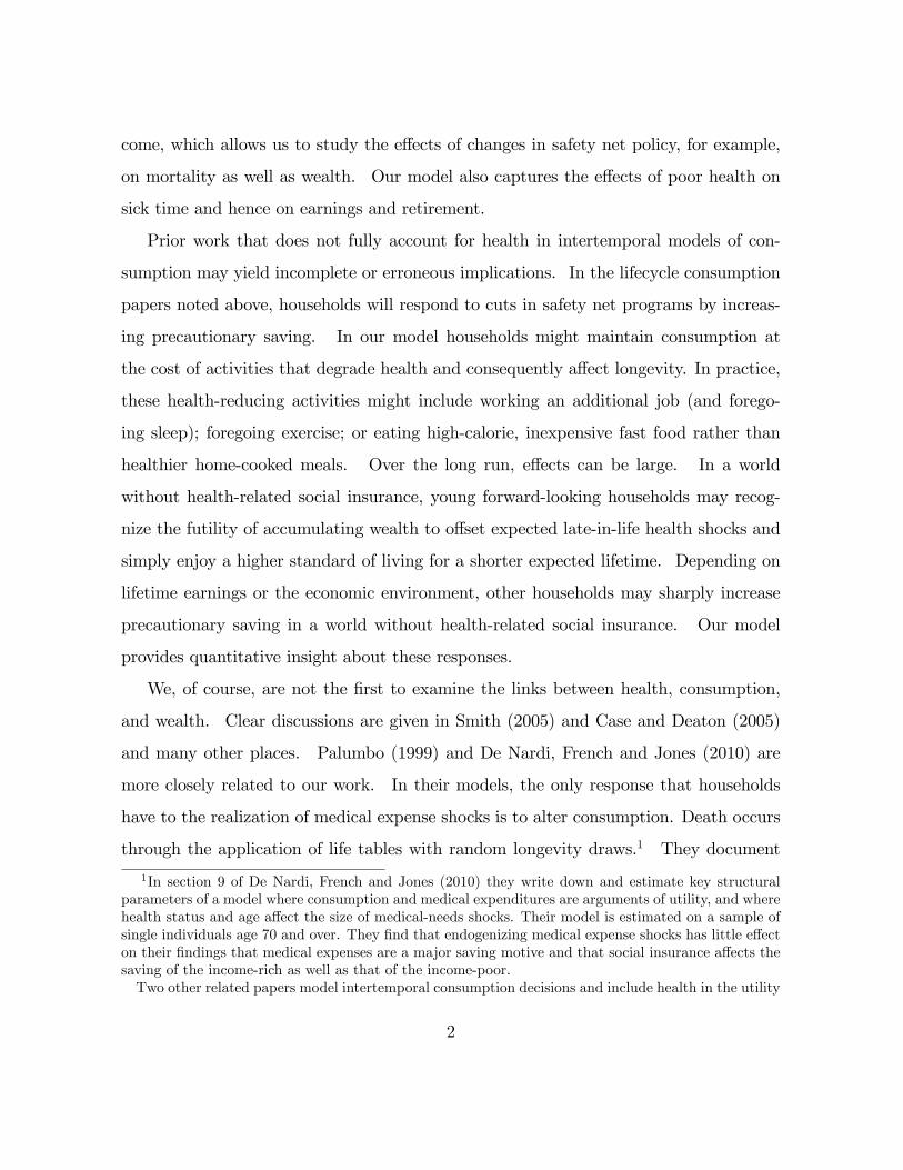
The third fact is "the gradient:" health is positively related to socioeconomic status,

whether measured by lifetime income, net worth, or related measures. As Figure 3 makes

clear, the positive relationship between self-reported health and net worth is strongly

present in the HRS. The Figure is similar when households are sorted by lifetime

income quintile. Illuminating economic decisions over the lifecycle that result in the

joint distribution of health and wealth, household-by-household, is a central challenge

5See, for example, Paffenbarger et al. (1993), Willette (1994), Mokdad et al. (2004), and Warburtonet al. (2006).

6

for this paper.

The fourth fact that our model must accommodate is that there is a strong relation-

ship between lifetime income and survival in the HRS. To show this, we restrict the

sample to birth years that, in principle, would allow someone to reach a specific age by

the last year of HRS data we have available, 2008. So, for example, when we look at

patterns of survival to age 70, we restrict the sample to those born before 1938. We

also drop all sample members who were over 60 years old in the year they entered the

HRS sample. The ten-year survival probabilities to age 70 shown in Figure 4 increase

monotonically with lifetime income, from 74 percent for men in the lowest lifetime in-

come quintile to 89 percent for men in the highest. The gradient for women goes from

79 percent in the lowest lifetime income quintile to 96 percent in the highest.

There are many likely explanations for the positive relationship between lifetime in-

come and survival. We write down and solve a model that captures several of these

explanations. Households in our model have different draws on annual earnings and

hence different lifetime incomes. They differ in the timing of exogenous marriage and

7

fertility. Given differences in incomes and demographic characteristics, their consump-

tion, health investments, and retirement choices will respond to health shocks (that vary

by age), earnings shocks (which are also affected by health), and government programs

in different ways. Moreover, we allow consumption and health to be gross complements

or gross substitutes in utility. The work that follows, therefore, illuminates the channels

through which health, consumption, and wealth are related.

3 Model Economy

We assume a household maximizes utility by choosing consumption, health investments,

and leisure. Time spent working depends on the health status of the individual (we

assume that sick time is related to the health stock) and rest of the time is divided

up between leisure and health investments. Retirement is endogenous. Even though

adding health capital and endogenous retirement involves only two additional choice

variables (relative to a standard life-cycle intertemporal consumption problem), it is

a significant complication. In addition to affecting longevity, households derive direct

8

satisfaction from health. Lifetime utility at any age, Vj, is given by an Epstein-Zin,

Kreps-Porteus formulation of recursive preferences

Vj = Maxc,l,h

[njU(cj/nj, lj, hj)

1−γ + β(EtV1−θj+1 )(1−γ)/(1−θ)

] 11−γ .

In the above formulation, θ measures the coeffi cient of risk aversion, 1γis the intertempo-

ral elasticity of substitution and U (·)1−γ denotes period utility which is non-separable

with the certainty equivalent of future utility. Notice that when θ = γ, we get the

standard time-additive separable case.

There are three related reasons we chose this specification of preferences. First,

it isolates the degree of risk aversion from the intertemporal elasticity of substitution.

These features of preferences may have independent effects on health and other household

choices. Second, as noted in Rosen (1988), with endogenous mortality, standard time-

additive preferences are not invariant to affi ne transformations. This arises due to the

fact that the household attributes zero utility to death and the agent needs to compare

the utility of any optimal schedule with zero to determine whether or not it is worthwhile

to live longer. Third, with common time-additive, separable CRRA preferences, U(c) =

c1−σ

1−σ , σ < 1 for utility to be a positive number. But most estimates and calibration

exercises suggest σ exceeds one. Our formulation allows σ to exceed one.6

The expectation operator Et denotes the expectation over uncertain future earnings

before retirement and uncertain health shocks throughout life, β is the discount factor,

j is age, c is consumption, and h is a composite stock of health for men and women in

the household, and l is leisure. nj is a household scale parameter and is a function of the

number of adults, A, and children, K, in the household, so n = g(Aj, Kj). Households

spend an indivisible amount of time ω(h) working each period and spend the rest of

their time endowment 1 − ω(h) on either leisure or on activities that augment health

6Hall and Jones (2007), following others, use conventional CRRA preferences but add a large enoughconstant to guarantee that utility is positive.

9

investments. We assume that ω(h) = ω−s(h) which draws from Grossman’s formulation

of sick time: households experience some loss in labor supply depending on sick time,

s(h), which is inversely related to their health status.7 Upon retirement, households

split their time endowment of 1 unit between leisure and health investments.

A challenge when modelling health is that there is at best mixed evidence that mar-

ginal expenditures on medical care in the U.S. buy greater health, and hence longevity.8

This phenomenon is sometimes referred to as “flat of the curve”medicine. It is notewor-

thy just how hard scholars need to look to find evidence that expenditures on medical

care have a discernible, positive effect on health and particularly mortality outcomes.

Card, Dobkin, and Maestas (2008), for example, is one of a small number of studies

that find expenditures are positively correlated with survival. Their work is based on a

very large sample of people admitted to emergency rooms in California: they find the

positive effects of spending apply to a small subset of the conditions that lead people

to show up in emergency rooms. Doyle (2010) shows that men who have heart attacks

when vacationing in Florida have higher survival probabilities if they end up being served

by high- rather than low-expenditure hospitals. Other studies suggest that marginal

medical expenditures have little discernible effect on health.

It is nevertheless clear that money can sometimes improve health. Antibiotics can

effectively cure strep throat. Treatment can help people survive cancer. A good ortho-

pedist can help people recover fully from broken bones. We assume that the household

7In our modeling of sick time, we assume that poor health adversely affects the time that an individualspends in the labor market. While poor health may well affect investments in human capital andconsequently the wage rate that an individual faces, we observe data on earnings and we do not observeeither hours worked or the wage rate. Consequently, data limitations prevent us from disentanglingthe impact of bad health on labor supply from its effect on hours worked. Furthermore, the analysisin French (2005) suggests that health status has a much larger impact on labor supply and labor forceparticipation than on the wage rate.

8See, for example, the Dartmouth Health Atlas (http://dartmouthatlas.org/), which documentslittle relationship between regional variation in health spending and health outcomes. Finkelstein andMcKnight (2008) find little effect of Medicare on mortality when the program was initiated. Chay,Kim and Swaminathan (2010) challenge this assessment.

10

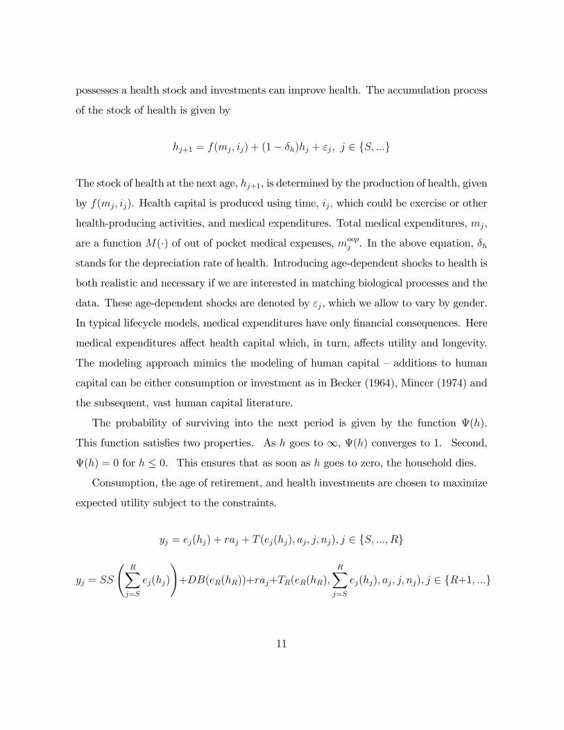
possesses a health stock and investments can improve health. The accumulation process

of the stock of health is given by

hj+1 = f(mj, ij) + (1− δh)hj + εj, j ∈ S, ...

The stock of health at the next age, hj+1, is determined by the production of health, given

by f(mj, ij). Health capital is produced using time, ij, which could be exercise or other

health-producing activities, and medical expenditures. Total medical expenditures, mj,

are a function M(·) of out of pocket medical expenses, moopj . In the above equation, δh

stands for the depreciation rate of health. Introducing age-dependent shocks to health is

both realistic and necessary if we are interested in matching biological processes and the

data. These age-dependent shocks are denoted by εj, which we allow to vary by gender.

In typical lifecycle models, medical expenditures have only financial consequences. Here

medical expenditures affect health capital which, in turn, affects utility and longevity.

The modeling approach mimics the modeling of human capital —additions to human

capital can be either consumption or investment as in Becker (1964), Mincer (1974) and

the subsequent, vast human capital literature.

The probability of surviving into the next period is given by the function Ψ(h).

This function satisfies two properties. As h goes to ∞, Ψ(h) converges to 1. Second,

Ψ(h) = 0 for h ≤ 0. This ensures that as soon as h goes to zero, the household dies.

Consumption, the age of retirement, and health investments are chosen to maximize

expected utility subject to the constraints.

yj = ej(hj) + raj + T (ej(hj), aj, j, nj), j ∈ S, ..., R

yj = SS

(R∑j=S

ej(hj)

)+DB(eR(hR))+raj+TR(eR(hR),

R∑j=S

ej(hj), aj, j, nj), j ∈ R+1, ...

11

cj + aj+1 +moopj = yj + aj − τ(ej(hj) + raj), j ∈ S, ..., R

cj + aj+1 +moopj = yj + aj − τ

(SS

(R∑j=S

ej(hj)

)+DB(eR(hR)) + raj

), j ∈ R+ 1, ...

In these expressions y is income, e(h) is earnings which depends on health stock, a is

assets, r is the interest rate, T is a transfer function, R is the age of retirement, and S

is the age that a household member enters the labor market. Social security (SS) is a

function of lifetime earnings, defined benefit pensions (DB) are a function of earnings

in the last year of life, τ is a payroll and income tax function, and the transfer function

for retirees (TR) is a function of social security, defined-benefit pensions, assets, age, and

family structure.

3.1 Retired Household’s Dynamic Programming Problem

A retired, married household between ages R and D obtains income from social security,

defined-benefit pensions, and preretirement assets. The dynamic programming problem

at age j for a retired household is given by

V (eR, ER, a, j, hh, hw) =

max

nU(c/n, 1− i, h)1−γ + βΨ(hh)Ψ(hw)[∫

εh

∫εw

V (eR, ER, a′, j + 1, h′h, h

′w)1−θdΞh(εh)dΞw(εw)

](1−γ)/(1−θ)

11−γ

subject to

y = SS(ER) +DB(eR) + ra+ TR(eR, ER, a, j, n)

c+ a′ +mooph +moop

w = y + a− τ(SS(ER), DB(eR) + ra)

12

h′h = F (M(mooph ), i) + (1− δh)hh + εh

h′w = F (M(moopw ), i) + (1− δh)hw + εw

h = ∆(hh, hw)

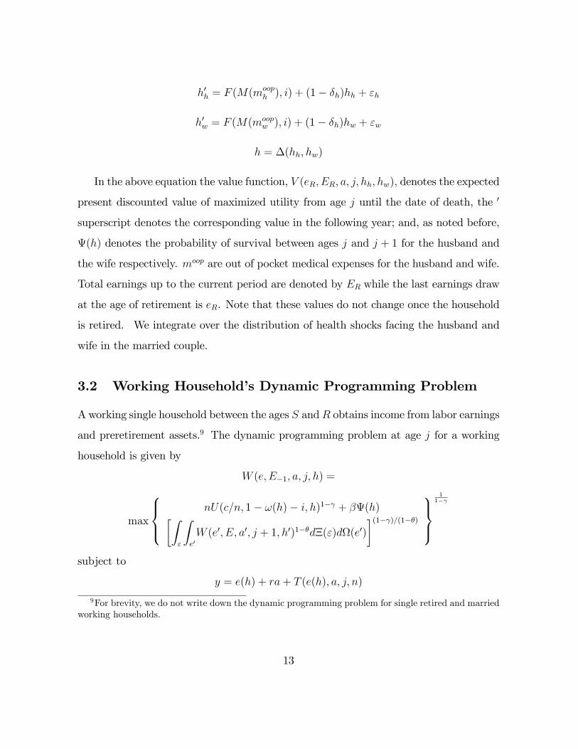
In the above equation the value function, V (eR, ER, a, j, hh, hw), denotes the expected

present discounted value of maximized utility from age j until the date of death, the ′

superscript denotes the corresponding value in the following year; and, as noted before,

Ψ(h) denotes the probability of survival between ages j and j + 1 for the husband and

the wife respectively. moop are out of pocket medical expenses for the husband and wife.

Total earnings up to the current period are denoted by ER while the last earnings draw

at the age of retirement is eR. Note that these values do not change once the household

is retired. We integrate over the distribution of health shocks facing the husband and

wife in the married couple.

3.2 Working Household’s Dynamic Programming Problem

Aworking single household between the ages S andR obtains income from labor earnings

and preretirement assets.9 The dynamic programming problem at age j for a working

household is given by

W (e, E−1, a, j, h) =

max

nU(c/n, 1− ω(h)− i, h)1−γ + βΨ(h)[∫

ε

∫e′W (e′, E, a′, j + 1, h′)1−θdΞ(ε)dΩ(e′)

](1−γ)/(1−θ)

11−γ

subject to

y = e(h) + ra+ T (e(h), a, j, n)

9For brevity, we do not write down the dynamic programming problem for single retired and marriedworking households.

13

c+ a′ +moop = y + a− τ(e(h) + ra)

h′ = F (M(moop), i) + (1− δh)h+ ε

E = E−1 + e(h)

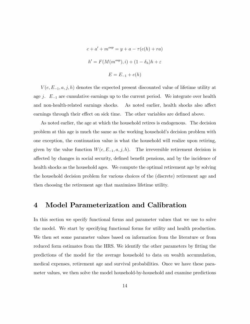
V (e, E−1, a, j, h) denotes the expected present discounted value of lifetime utility at

age j. E−1 are cumulative earnings up to the current period. We integrate over health

and non-health-related earnings shocks. As noted earlier, health shocks also affect

earnings through their effect on sick time. The other variables are defined above.

As noted earlier, the age at which the household retires is endogenous. The decision

problem at this age is much the same as the working household’s decision problem with

one exception, the continuation value is what the household will realize upon retiring,

given by the value function W (e, E−1, a, j, h). The irreversible retirement decision is

affected by changes in social security, defined benefit pensions, and by the incidence of

health shocks as the household ages. We compute the optimal retirement age by solving

the household decision problem for various choices of the (discrete) retirement age and

then choosing the retirement age that maximizes lifetime utility.

4 Model Parameterization and Calibration

In this section we specify functional forms and parameter values that we use to solve

the model. We start by specifying functional forms for utility and health production.

We then set some parameter values based on information from the literature or from

reduced form estimates from the HRS. We identify the other parameters by fitting the

predictions of the model for the average household to data on wealth accumulation,

medical expenses, retirement age and survival probabilities. Once we have these para-

meter values, we then solve the model household-by-household and examine predictions

14

for each household in our sample.

Preferences: Recall that preferences are recursive. We assume that momentary

household utility has a constant relative risk-averse form. We further assume the subu-

tility function over consumption and health has a constant elasticity of substitution.

Hence the period utility takes the form

U(c/n, h, l)1−γ = [λ(cηl1−η

)ρ+ (1− λ)hρ]

1−γρ .

The elasticity of substitution between the consumption-leisure composite and health is

1/(1− ρ). The parameter γ is the inverse of the intertemporal elasticity of substitution.

The discount factor (β) is set at 0.96, a value similar to the 0.97 value used in Hubbard,

Skinner, and Zeldes (1995); and Engen, Gale, and Uccello (1999). We also set η = 0.36

from Cooley and Prescott (1995). Finally, we set θ, the coeffi cient of risk aversion equal

to 3, a value commonly used in many studies including Hubbard, Skinner, and Zeldes

(1995). We calibrate γ.

Health aggregator : Our analysis of consumption and wealth accumulation is nat-

urally at the household level. But health is clearly individual. We model individual

investments in health that we then aggregate to the household level using a simple CES

function

h = Υ(hh, hw) = [ϑ (hh)υ + (1− ϑ) (hw)υ]

1υ .

Equivalence Scale: This is obtained from Citro and Michael (1995) and takes the

form

n = g(A,K) = (A+ 0.7K)0.7

where A indicates the number of adults and K indicate the number of children in the

household.

Rate of Return: We assume an annualized real rate of return, r, of 4 percent. This

15

assumption is consistent with McGrattan and Prescott (2003), who find that the real

rate of return for both equity and debt in the United States over the last 100 years, after

accounting for taxes on dividends and diversification costs, is about 4 percent.

Taxes: We model an exogenous, time-varying, progressive income tax that takes a

form used by Gouveia and Strauss (1994, 1999)

τ(y) = a(y − (y−a1 + a2)−1/a1),

where y is in thousands of dollars. We estimate parameters a, a1, and a2 using informa-

tion on taxes paid and incomes by income class drawn from Statistics of Income volumes

(produced by the Internal Revenue Service) available electronically through the Boston

Public Library. The function characterizes U.S. effective, average household income tax

rates between 1950 and 2008.

Earnings and Earnings Expectations: Earnings data through 2007 come from three

sources: Social Security Administration Summary Earnings files, SSA earnings detail

files (W2 information), and HRS self-reports.

Earnings in the Summary Earnings files are top-coded. Starting in 1978 we have

un-top-coded W2 data for many individuals. Starting in 1992 we have HRS self-reports

of earnings. If available, we use W2 data or self-reports to address top-coding. For

top-coded observations from 1951 to 1977, we estimate a censored regression model

to predict true earnings for top-coded observations.10 For the remaining top-coded

observations from 1978 to 2007 we use a similar empirical model, adding labor force

status to the covariates after 1992. We set missing earnings to zero in years following

10The empirical model includes the following covariates: gender, education, birth year, race, censusregion, marital status, average percentile in the earnings distribution over the previous 5 years (ifavailable), average percentile in the earnings distribution over the next 5 years (if available), numberof children in the household, total years reported working, and average real household wealth over theHRS study years (1992,1994,. . . 2008). The non-time-varying covariates are drawn from the first wavethe respondent appears in the HRS.

16

the respondent’s last year of work or retirement year, for respondents who report never

having worked, and for respondents younger than age 17. We impute the remaining

missing earnings using a variant of our empirical earnings model: rather than using

the respondent’s percentile in the earnings distribution, we use the respondent’s average

real earnings in the past/next five years.

Earnings expectations are a central influence on life-cycle consumption and health

accumulation decisions, both directly and through their effects on expected pension and

social security benefits.11 We aggregate individual earnings histories into household

earnings histories, putting earnings in constant dollars using the CPI-U. The household

model of log earnings (and earnings expectations) is

log ej = αi + β1AGEj + β2AGE2j + uj

uj = ρuj−1 + εj

where, as mentioned above, ej is the observed earnings of the household i at age j in 2008

dollars, αi is a household specific constant, AGEj is age of the head of the household, uj

is an AR(1) error term of the earnings equation, and εj is a zero-mean i.i.d., normally

distributed error term. The estimated parameters are αi, β1, β2, ρ and σε.

We divide households into six groups according to education, marital status and

the number of earners in the household, resulting in six sets of household-group-specific

parameters, which we then estimate separately for each of the five HRS cohorts (resulting

in 30 sets of parameters).12 Estimates of the persistence parameter, ρ, across groups

11Due to data and computational limitations, we assume that earnings expectations are independentof health status. Credibly relaxing this assumption would require data on wage rates, hours, and healthprior to when households enter the HRS.12The groups are (1) married, head without a college degree, one earner; (2) married, head without a

college degree, two earners; (3) married, head with a college degree, one earner; (4) married, head witha college degree, two earners; (5) single without a college degree; and (6) single with a college degree.We estimate the parameters separately for the AHEAD, CODA, HRS, War Babies, and Early Boomercohorts. A respondent is an earner if his or her lifetime earnings are positive and contribute at least

17

range from 0.69 to 0.82.

Assuming a 40 hour workweek and 112 hours of non-sleeping time per week, we set

the value of full-time work, ω, to 0.36.

Transfer Programs: We model public income transfer programs using the specifica-

tion in Hubbard, Skinner and Zeldes (1995). Specifically, the transfer that a household

receives while working is given by

T = max0, c− [e+ (1 + r)a]

whereas the transfer that the household receives upon retiring is

T = max0, c− [SS(ER) +DB(eR) + (1 + r)a]

This transfer function guarantees a pre-tax income of c and implies that earnings,

retirement income, and assets reduce public benefits dollar for dollar. To set c we use

information from Moffi tt (2002) for 1960, 1964, 1968 to 1998 and extend the series using

data from The Urban Institute, Mathematica Policy Research Inc., Center for Medicare

and Medicaid Services, and the UKCPR National Welfare Data.13 These data are at

the state level so we take a weighted average according to state population in each year.

Benefits have trended down since 1974 when the consumption floor for a single parent,

two-child family peaked at $14,767 (in year 2008 dollars). In 2007 the same family would

have received transfers worth $11,308.

Defined benefit pensions: Pension expectations and benefits come from an empirical

defined-benefit pension function estimated with HRS data. The function includes indi-

cator variables for having a defined benefit plan and belonging to a union, and variables

for years in the pension by the retirement date, household earnings in the last year of

20 percent of the lifetime earnings of the household.13See http://www.ukcpr.org/AvailableData.aspx

18

work and the fraction of household earnings earned by the male and the fraction earned

by the female.

Health production: We assume that the production of health is given by F (M(m), i) =

At (mχi1−χ)ξ, where total medical expenses are a function of out-of-pocket expenses,

m = M(moop) and health is also produced with time, i. We assume At grows at 3

percent per year reflecting aggregate improvements in productivity of health technol-

ogy. Total medical expenditures are related to out-of-pocket expenditures by a linear

function that depends on insurance status. For the uninsured this function takes the

form, m =

moop + c, shock

moop, no shock. In the absence of a health shock, health care ex-

penditures come directly out of the uninsured household’s pocket. In the event that

the uninsured household suffers an adverse health shock, a baseline level of care, c, is

provided via charity care.

For an insured household, total medical expenses are paid partially out of pocket

and partially through insurance, m = D + ζ(m−D)︸︷︷︸OOP

+ (1− ζ)(m−D)︸︷︷︸insurance

. There are two

parts of out-of-pocket expenses, the deductible D and a fraction ζ ∈ [0, 1] of the balance,

(m−D), that remains after the deductible has been paid.

We use the Medical Expenditure Panel Survey (MEPS) to calibrate the parameters

of the medical expense model for six different insurance categories. Households in which

the head is younger than 65 may be: uninsured, insured with public insurance only, or

insured with any sort of private insurance. Three more categories capture older house-

holds: Medicare only, Medicare with supplemental public insurance (but no private), or

Medicare and any private insurance.

To calibrate the value of charity care for the uninsured, we draw from Doyle (2005)

who suggests the previous estimates "center around forty percent less care for the unin-

sured."14 The average total medical spending for the insured (under age 65) in the

14See, for example, Currie and Gruber (1997), Currie and Thomas (1995), Haas and Goldman (1994),

19

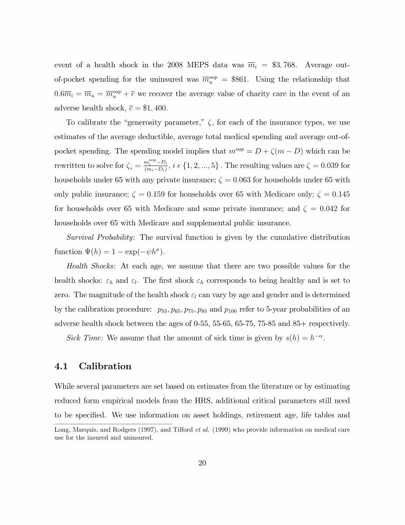
event of a health shock in the 2008 MEPS data was mi = $3, 768. Average out-

of-pocket spending for the uninsured was moopu = $861. Using the relationship that

0.6mi = mu = moopu + c we recover the average value of charity care in the event of an

adverse health shock, c = $1, 400.

To calibrate the “generosity parameter,” ζ, for each of the insurance types, we use

estimates of the average deductible, average total medical spending and average out-of-

pocket spending. The spending model implies that moop = D+ ζ(m−D) which can be

rewritten to solve for ζ i =moopi −Di(mi−Di) , i ε 1, 2, ..., 5 . The resulting values are ζ = 0.039 for

households under 65 with any private insurance; ζ = 0.063 for households under 65 with

only public insurance; ζ = 0.159 for households over 65 with Medicare only; ζ = 0.145

for households over 65 with Medicare and some private insurance; and ζ = 0.042 for

households over 65 with Medicare and supplemental public insurance.

Survival Probability: The survival function is given by the cumulative distribution

function Ψ(h) = 1− exp(−ψhσ).

Health Shocks: At each age, we assume that there are two possible values for the

health shocks: εh and εl. The first shock εh corresponds to being healthy and is set to

zero. The magnitude of the health shock εl can vary by age and gender and is determined

by the calibration procedure: p55, p65, p75, p85 and p100 refer to 5-year probabilities of an

adverse health shock between the ages of 0-55, 55-65, 65-75, 75-85 and 85+ respectively.

Sick Time: We assume that the amount of sick time is given by s(h) = h−α.

4.1 Calibration

While several parameters are set based on estimates from the literature or by estimating

reduced form empirical models from the HRS, additional critical parameters still need

to be specified. We use information on asset holdings, retirement age, life tables and

Long, Marquis, and Rodgers (1997), and Tilford et al. (1999) who provide information on medical careuse for the insured and uninsured.

20

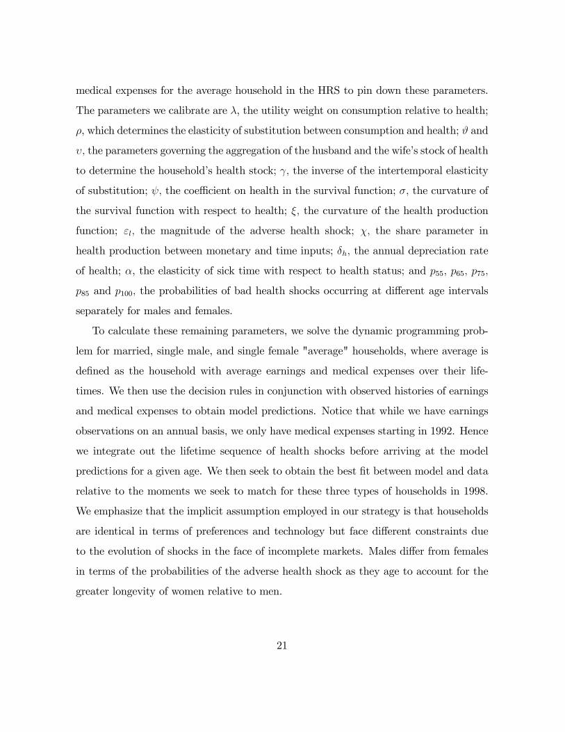
medical expenses for the average household in the HRS to pin down these parameters.

The parameters we calibrate are λ, the utility weight on consumption relative to health;

ρ, which determines the elasticity of substitution between consumption and health; ϑ and

υ, the parameters governing the aggregation of the husband and the wife’s stock of health

to determine the household’s health stock; γ, the inverse of the intertemporal elasticity

of substitution; ψ, the coeffi cient on health in the survival function; σ, the curvature of

the survival function with respect to health; ξ, the curvature of the health production

function; εl, the magnitude of the adverse health shock; χ, the share parameter in

health production between monetary and time inputs; δh, the annual depreciation rate

of health; α, the elasticity of sick time with respect to health status; and p55, p65, p75,

p85 and p100, the probabilities of bad health shocks occurring at different age intervals

separately for males and females.

To calculate these remaining parameters, we solve the dynamic programming prob-

lem for married, single male, and single female "average" households, where average is

defined as the household with average earnings and medical expenses over their life-

times. We then use the decision rules in conjunction with observed histories of earnings

and medical expenses to obtain model predictions. Notice that while we have earnings

observations on an annual basis, we only have medical expenses starting in 1992. Hence

we integrate out the lifetime sequence of health shocks before arriving at the model

predictions for a given age. We then seek to obtain the best fit between model and data

relative to the moments we seek to match for these three types of households in 1998.

We emphasize that the implicit assumption employed in our strategy is that households

are identical in terms of preferences and technology but face different constraints due

to the evolution of shocks in the face of incomplete markets. Males differ from females

in terms of the probabilities of the adverse health shock as they age to account for the

greater longevity of women relative to men.

21

The moments we use to identify and pin down the parameters are:15

1. Mean net worth in 1998 for married couples (husband age 63.2, wife age 60.9) is

$508,904

2. Mean net worth in 2008 for married couples is $628,599

3. Mean net worth in 1998 for single males (age 64.1) is $295,486

4. Mean net worth in 1998 for single females (age 66.7) is $193,064

5. The probability of dying between ages 50-54 for males: 3.08%




9. The probability of dying between ages 50-54 for females: 1.834%




13. Average annual total medical expenses for married women age 19-44: $4,454

15Moments for net worth data and the retirement age come directly from HRS data. Mo-ments for total medical expenses come from the National Health Expenditure Accounts (usingthe personal health spending totals by age for 2004), drawn from http://www.cms.gov/Research-Statistics-Data-and-Systems/Statistics-Trends-and-Reports/NationalHealthExpendData/Age-and-Gender-Items/CMS1242122.html. We disaggregate the National Health Expenditure Account totalfor married men, married women, single men, and single women using data from the MedicalExpenditure Panel Study. The mortality probabilities come from the World Health Organization,http://www.who.int/healthinfo/statistics/mortality_life_tables/en/. The data on sick hours comefrom the PSID.

22




17. Average annual total medical expenses for married women age 80+: $17,896

18. Average annual total medical expenses for single women age 70-74: $12,479

19. Average annual total medical expenses for married men age 70-74: $13,225

20. Average annual total medical expenses for single men age 70-74: $13,474

21. Sick hours relative to total work hours at age 40: 0.015

22. Retirement Age: 62

The model with each calibrated parameter generates 22 non-linear equations with

22 unknowns. We obtained an exact match between the model predictions and the

moments listed above. The resulting parameter values are given below.

Parameter λ ρ ϑ υ γ

Value 0.71 -4.1 0.49 0.73 0.78

Parameter ψ σ ξ εl χ

Value .0012 1.53 0.69 -14.4 0.49

Parameter p55 p65 p75 p85 p100 δh

Value 0.06 0.11 0.139 0.197 0.245 0.042

Parameter p55,f p65,f p75,f p85,f p100,f α

Value 0.04 0.09 0.119 0.168 0.229 0.17The value of γ is equal to 0.78, which implies an intertemporal elasticity of substi-

tution (1/γ) of 1.28. This number is not comparable with the Euler equation based

23

estimates of the IES since most studies estimating the IES use standard time addi-

tively separable preferences. The elasticity of substitution between consumption/leisure

composite and health is 11−ρ = 0.2. Consumption and health are complements and our

calibrated value is very close to the estimates in Finkelstein, Luttmer, and Notowidigdo

(forthcoming). In a married household, the male and the female’s health are very good

substitutes as reflected by υ = 0.73. The rate of depreciation of health is 4.2 percent per

year. The share of goods in the production of health χ is 0.49, suggesting that time and

goods are both important in the production of health. The bad health shock, εl, takes

on the value -14.4 (recall that the good health shock εh is set to 0). Finally, note that

the 5-year realization probability of the bad health shock increases from 6 percent for

men (4 percent for women) below 55 years of age to 11 percent (9 percent for women)

for men between 55 and 65, to 13.9 percent (11.9 percent for women) for men between

65 and 75, to 19.7 percent (16.8 percent for women) for households between 75 and 85,

and to 24.5 percent (22.9 percent for women) for men above the age of 85.

As mentioned above, we match 22 data moments with the model to identify these

22 parameters. Clearly, altering one of the target data moments changes more than one

parameter. Nevertheless, it is instructive to think about which data moments play a

critical role for at least some of the more important parameters.

A lower value of ρ will lead to a higher level of assets in 1998. In addition, a

lower value of ρ will have implications for asset accumulation/decumulation late in life.

Predictable declines in health ought to be associated with predictable declines in con-

sumption. Hence having asset levels in 1998 as well as 2008 helps pin down ρ.

The parameters governing the production technology for health (for males) as well

as the hazard function are pinned down by the mortality probabilities as well as medical

expenses. Recall that health affects both utility as well as mortality. The importance of

health in utility (λ) as well as the significance of health in improving longevity are both

simultaneously pinned down by these moments. The probabilities of dying as people age

24

interact with the technology for producing health to determine medical expenses. For

instance if diminishing returns set in quickly, substantial medical expenses need to be

expended simply to maintain the stock of health. In contrast, if the medical technology

were close to linear, then additional medical expenses will have a large effect on the stock

of health. Hence, all these objects (medical technology parameters, importance of health

relative to consumption in utility), as well as the parameters of the hazard function, are

simultaneously pinned down by the probabilities of the bad shock and medical expenses

as men age.

Medical expenses for single women and probabilities of dying for men relative to

women help pin down the probabilities of bad health shocks for women. In addition,

mean net worth for singles relative to married couples shed light on the health aggregator

in preferences. A change in the parameters governing the health aggregator for married

households (ϑ, υ) will affect both the wealth of the married household as well as medical

expenses for married women relative to single women.

4.2 Model Solution

With the calibrated parameters, we solve the dynamic programming problem by lin-

ear interpolation on the value function. For each household in our sample we compute

optimal decision rules for assets and the stock of health from the oldest possible age

(assumed to be 120) to the beginning of working life (S) for any feasible realizations of

the random variables: earnings and health shocks. These decision rules differ for each

household, since each faces stochastic draws from different earnings distributions (recall

they are household specific). Household-specific earnings expectations also directly influ-

ence expectations about social security and pension benefits. Other characteristics also

differ across households. We then use the decision rules and the observed earnings and

medical expenses to obtain the model’s predictions for wealth, health, medical expenses

and mortality at a given age. Where we do not have annual data on medical expenses

25

or earnings, we use the distributions of earnings shocks or health shocks to integrate out

expected medical expenses and earnings.

5 Results

As emphasized in the previous discussion, we calibrate key model parameters to the

average (married, single male and single female-headed) HRS household in 1998. The

first question we address, therefore, is how the model matches household wealth, out

of pocket medical expenses, and the stock of health. We summarize results for house-

hold wealth and out-of-pocket medical expenses by showing median values, breaking

households into lifetime income quintiles.16

Table 1: Median Net Worth and Out-of-Pocket Medical Expenditures, Model and Data, 1998 and 2008

1998 Median Net Worth Median OOP Medical Expenses

Lifetime Income Data Model Data Model

Lowest Quintile $33,588 $23,596 $708 $735

Second Quintile 60,717 47,506 904 845

Middle Quintile 97,212 94,503 995 956

Fourth Quintile 180,859 151,203 930 982

Highest Quintile 340,144 322,309 1,023 1,012

2008

Lowest Quintile $15,495 $15,283 $640 $632

Second Quintile 63,900 57,495 1,080 921

Middle Quintile 136,000 127,503 1,200 1,146

Fourth Quintile 238,000 253,991 1,384 1,323


16Lifetime income is defined within four roughly equal-sized age groups: under 60, 60 to 65, 66 to75, and over 75.

26

There are two striking features of Table 1. First, while we calibrate the model to

the average household in 1998, the model does a good job matching the wide variation

in wealth across low and high lifetime income households in 1998. The correlation of

actual and optimal net worth in 1998 is 0.69. Scholz, Seshadri, and Khitatrakun (2006)

report a correlation between model predications and net worth in the HRS of 0.86 in

1992. There are a number of differences between our earlier work and this paper. The

most important is that health affects utility and longevity, households make endogenous

health investments, we model the health decisions of spouses, retirement is endogenous,

preferences are not time-additively separable, new cohorts have been added to the data

and we now look at a much more recent period, and we have new estimates of the earning

process, which show somewhat more volatility in earnings than our previous estimates,

among other changes. Despite these differences our earlier qualitative conclusion still

holds: Most Americans seem to be preparing well for financially secure retirements.

Predicted out-of-pocket median medical expenses also match actual expenses fairly

closely. For instance, in 1998, the out of pocket medical expenses rise from $735 for the

lowest lifetime income quintile to $1,012 for the highest income quintile. This tracks the

data pretty closely. Richer households spend more out of pocket (despite possessing

better health on average at the same age) and these investments affect both flow utility as

well as longevity. The household-by-household correlation between actual out-of-pocket

medical expenditures and optimal out-of-pocket medical expenditures in the model is

0.50.

The second striking feature of Table 1 is the degree to which we match the dispersion

of median net worth and out-of-pocket medical expenditures by lifetime income quin-

tile in 2008. We use only one net worth moment for 2008 (the net worth of married

couples): health expenses are for 2004 (due to the timing of the National Health Ex-

penditure Accounts). Yet the behavioral model augmented with preference parameters

calibrated to the average household in 1998, data on changes in household composition,

27

and earnings realizations (for those still in the labor market) is able to closely match

the 2008 distribution of median net worth and out—of-pocket health spending.

Another feature of the HRS are questions on self reported health status, which we

used in Figures 1 and 3. Households report this on a 5 point scale ranging from poor

to excellent. In the model, the stock of health is a continuous variable and hence to

compare with the data, we turn the continuous health variable into a discrete one. In

the HRS data, 13 percent of the sample report excellent health, 28 percent report very

good, 30 percent report good, 19 percent report fair and 9 percent report poor. We

choose the cut-off points in the continuous distribution so that these percentages are

what we observe in the HRS. Table 2 depicts the connection between the model and

data for 1998 and 2008 in more detail.Table 2: Self-reported Health Status, Model and Data, 1998 and 2008

Fraction of Households by Self Reported Health Status

Lifetime Income Excellent V. Good Good Fair Poor

1998 Data Model Data Model Data Model Data Model Data Model

Bottom Quintile 7 7 17 15 28 29 28 29 19 18

Second Quintile 10 9 20 21 28 26 26 27 16 17

Middle Quintile 12 12 23 22 33 34 21 20 11 12

Fourth Quintile 13 14 29 28 34 33 18 19 7 6

Highest Quintile 18 19 36 35 30 29 12 12 4 5

2008

Bottom Quintile 5 6 18 19 28 27 31 30 18 18

Second Quintile 7 7 22 21 31 30 26 27 13 15

Middle Quintile 9 10 26 24 33 32 23 24 9 10

Fourth Quintile 10 10 32 31 33 32 19 19 7 8


There is a very tight link between lifetime income and the self-reported health status

28

and the model does an excellent job at tracking the variation in the data. Various

model features come into play here - as households age, they receive adverse shocks

with greater intensity. Their ability to buffer these shocks depends largely on health

investments they had made in the past (which determines their current health status)

as well as their income. The pace at which health deteriorates in older ages also affects

consumption (recall that consumption and health are complements) which in turn affects

wealth accumulation. The fact that the model is able to match the extent to which

health worsens between 1998 and 2008 adds to our confidence that the model provides

a reasonable description of the evolution of health by lifetime income.

A final feature of our model is retirement. Recall that the decision to retire is

endogenous. Table 3 gives the fit between model and data on retirement age.

Table 3: Retirement Age, Model Prediction and HRS Data

Median Retirement Age by Self Reported Health Status

Lifetime Income Excellent V. Good Good Fair Poor

Data Model Data Model Data Model Data Model Data Model

Bottom Quintile 61 60 61 61 60 59 57 58 54 55

Second Quintile 60 61 63 62 62 61 61 61 57 57

Middle Quintile 62 62 62 62 62 62 60 61 60 59

Fourth Quintile 62 62 62 63 62 63 62 62 61 60


In the data, low lifetime income households with poor health status retire early (age

54) while the majority of households retire at 62. The early retirement of poor households

is triggered by the early onset of bad health shocks. These households typically have low

earnings options and hence choose to retire early. Richer households who have better

health expect to live longer and hence choose to retire later, partly to finance a longer

retirement period.

29

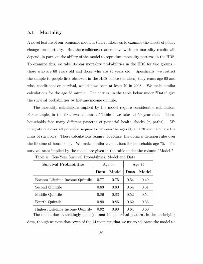
5.1 Mortality

A novel feature of our economic model is that it allows us to examine the effects of policy

changes on mortality. But the confidence readers have with our mortality results will

depend, in part, on the ability of the model to reproduce mortality patterns in the HRS.

To examine this, we take 10-year mortality probabilities in the HRS for two groups —

those who are 60 years old and those who are 75 years old. Specifically, we restrict

the sample to people first observed in the HRS before (or when) they reach age 60 and

who, conditional on survival, would have been at least 70 in 2008. We make similar

calculations for the age 75 sample. The entries in the table below under "Data" give

the survival probabilities by lifetime income quintile.

The mortality calculations implied by the model require considerable calculation.

For example, in the first two columns of Table 4 we take all 60 year olds. These

households face many different patterns of potential health shocks (εl paths). We

integrate out over all potential sequences between the ages 60 and 70 and calculate the

mass of survivors. These calculations require, of course, the optimal decision rules over

the lifetime of households. We make similar calculations for households age 75. The

survival rates implied by the model are given in the table under the column "Model."

Table 4: Ten-Year Survival Probabilities, Model and Data

Survival Probabilities Age 60 Age 75

Data Model Data Model

Bottom Lifetime Income Quintile 0.77 0.75 0.54 0.49

Second Quintile 0.83 0.80 0.54 0.51

Middle Quintile 0.86 0.83 0.52 0.54

Fourth Quintile 0.90 0.85 0.62 0.56

Highest Lifetime Income Quintile 0.92 0.88 0.64 0.60The model does a strikingly good job matching survival patterns in the underlying

data, though we note that seven of the 14 moments that we use to calibrate the model tie

30

down mortality probabilities by age for households with average lifetime incomes. This

does not, however, imply that we would expect the model to reproduce survival patterns

for high- or low-lifetime income quintile households. Both at age 60 and 75, there are

substantial deviations between the survival data and predictions for households in the

highest lifetime income quintiles. These are likely to be the households that are most

effi cient in producing health capital. At age 75 there is also a substantial deviation

between data and model in the lowest lifetime income quintile. This is the pattern we

expect to see as unobservable effi ciency in health investment should make low-income

households in the HRS who survive to age 75 healthier than the average low-income

households in the model.

5.2 Complementarity

The degree of complementarity between consumption and health in the utility function

plays a central role in understanding our results. In Table 5 we illustrate the effect

of setting ρ to zero (which would make the consumption-leisure composite and health

separable in the utility function) on optimal net worth.

Table 5: The Effect of Complementarity on Optimal Wealth Accumulation, 1998

Median Net Worth

Baseline Model (ρ = −4.1) ρ = 0

Bottom Quintile $23,596 $48,485

Second Quintile 47,506 104,507

Middle Quintile 94,503 157,120

Fourth Quintile 151,203 322,346

Highest Quintile 322,309 532,340When consumption and health are complements in the utility function, households

anticipate that as health declines late in life, so will consumption. This phenomenon

is absent when consumption and health are separable in preferences. Hence the model

31

with complementarity will, all else equal, imply less asset accumulation than when ρ

equals zero. Other moments are also affected. To illustrate this, we set ρ to zero and

re-calibrate the model. We ignore the 2008 wealth moment and solve 21 equations in

21 unknowns. We then re-do simulations for all households in the sample. We report

below the fit of the model (baseline in parenthesis)

1. The correlation between model and data for net worth in 1998: 0.48 (0.69)

2. The correlation between model and data for out-of-pocket medical expenses in

1998: 0.31 (0.50)

3. The model correctly predicts the exactly stock of health (on a 5-point scale) for

48 (72) percent of the population in 1998

Complementarity has an important effect on the fit of the model for net worth,

out-of-pocket medical expenses, and the stock of health.

Another way to illustrate the importance of consumption-health complementarity is

to examine changes in wealth between 1998 and 2008. As individuals age, health deteri-

orates. A sceptic might be worried that this deterioration in health might be associated

with too steep a change in wealth when health and consumption are complements. To

examine this, we compute the ratio of wealth in 2008 to wealth in 1998 for each house-

hold that is alive in 2008. We then proceed to arrange them by lifetime income quintile

and report the median ratio in Table 6.

32

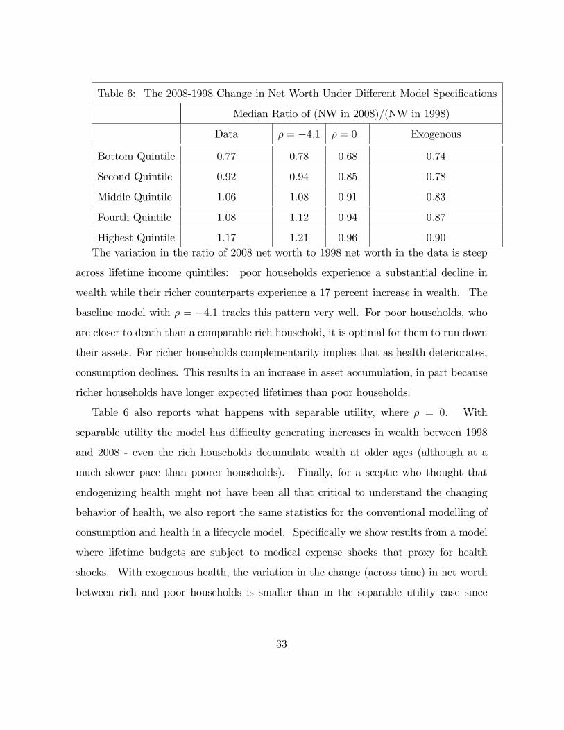
Table 6: The 2008-1998 Change in Net Worth Under Different Model Specifications

Median Ratio of (NW in 2008)/(NW in 1998)

Data ρ = −4.1 ρ = 0 Exogenous

Bottom Quintile 0.77 0.78 0.68 0.74

Second Quintile 0.92 0.94 0.85 0.78

Middle Quintile 1.06 1.08 0.91 0.83

Fourth Quintile 1.08 1.12 0.94 0.87

Highest Quintile 1.17 1.21 0.96 0.90The variation in the ratio of 2008 net worth to 1998 net worth in the data is steep

across lifetime income quintiles: poor households experience a substantial decline in

wealth while their richer counterparts experience a 17 percent increase in wealth. The

baseline model with ρ = −4.1 tracks this pattern very well. For poor households, who

are closer to death than a comparable rich household, it is optimal for them to run down

their assets. For richer households complementarity implies that as health deteriorates,

consumption declines. This results in an increase in asset accumulation, in part because

richer households have longer expected lifetimes than poor households.

Table 6 also reports what happens with separable utility, where ρ = 0. With

separable utility the model has diffi culty generating increases in wealth between 1998

and 2008 - even the rich households decumulate wealth at older ages (although at a

much slower pace than poorer households). Finally, for a sceptic who thought that

endogenizing health might not have been all that critical to understand the changing

behavior of health, we also report the same statistics for the conventional modelling of

consumption and health in a lifecycle model. Specifically we show results from a model

where lifetime budgets are subject to medical expense shocks that proxy for health

shocks. With exogenous health, the variation in the change (across time) in net worth

between rich and poor households is smaller than in the separable utility case since

33

medical expenses do not influence longevity.17 We conclude that the assumed degree of

complementarity is reasonable and plays an important role in explaining the behavior

of mortality, health, medical expenses as well as health for older households.

5.3 Medicare and Longevity

Policy simulations are another way to gain insight into behavior and the way our model

works. In Table 7 we examine the effect of removing our stylized version of Medicare,

the universal social insurance program that was established in 1965 to provide health

insurance to the elderly. Our modeling of this change is extreme: instead of being

eligible for a Government-provided insurance program upon reaching age 65, households

are uninsured.18 There are several reasons why we focus on this policy. First, Medicare

is a massive social insurance program costing $325 billion in fiscal year 2006. Second,

end-of-life health shocks have been shown by several authors to have significant effects on

asset accumulation. Third, Finkelstein and McKnight (2008) show in the first 10 years

following the establishment of Medicare, there was no discernible effect on mortality,

though Chay et al. (2010) challenge this conclusion. The effects of policy changes

on mortality and asset accumulation in the short- and long-run are issues the model is

nicely designed to address.

Suppose that Medicare were instantly eliminated in 1998 and the change was not an-

17Indeed, even the recent work of Denardi et al. (2010) has a diffi cult time rationalizing the increasein asset holdings of rich singles. While their model does a very nice job explaining the behavior ofthe bottom quintiles, the top quintile experiences an increase in assets late in life while their modelgenerates a decline over the same time period. Recall that our sample also includes married householdswho are richer on average than single households. This, in large measure, explains why even our averagehousehold experiences an increase in asset holdings while in their sample, the average household doesnot.18As noted earlier, medical care for insured households ism = D + ζ(m−D)︸︷︷︸

OOP

+(1− ζ)(m−D)︸︷︷︸insurance

. Total

medical expenditures for the uninsured are m =

moop + c, shockmoop, no shock

. This policy experiment is

extreme in the sense that institutions would undoubtedly evolve to provide insurance opportunities forthe elderly.

34

ticipated. All assets and health capital held by households had been accumulated under

the assumption that Medicare would exist. Medicare is financed by taxes on earned in-

come and so when Medicare is eliminated, we rebate annually back to the household

all future Medicare tax payments. After eliminating Medicare, we can recompute the

model and examine the effects on 10-year survival probabilities.

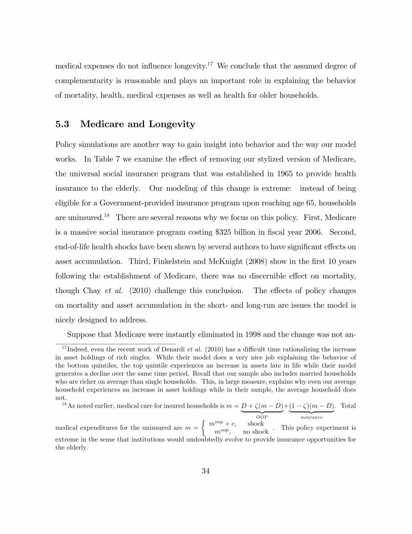
Table 7 shows the short-run effect on mortality (under the "No Med" column) of

eliminating Medicare are sizeable. Since most accumulation of health capital and wealth

occurs well before retirement, health status is largely fixed by age 60-65. Eliminating

Medicare, therefore, has little effect on health in the years immediately following its

repeal. Nevertheless, Medicare provides insurance against health shocks and given

that Medicare was eliminated unexpectedly, households did not have an opportunity to

increase their savings in order to self insure.

Table 7: Short- and Long-Run Effects of Eliminating Our Stylized Medicare Program

Age 60 Age 75

Lifetime Income Baseline No Med LR Baseline No Med LR

Bottom 0.75 0.71 0.66 0.49 0.45 0.40

Second 0.80 0.74 0.71 0.51 0.46 0.43

Middle 0.83 0.79 0.77 0.54 0.50 0.48

Fourth 0.85 0.81 0.81 0.56 0.53 0.52

Highest 0.88 0.84 0.85 0.60 0.57 0.58

There are three primary effects of removing Medicare. The first is the insurance

effect, the fact that Medicare provides insurance against health shocks. The second is

the investment effect, the idea that individuals are more likely to invest more in health

when young if they know there is insurance available at older ages. Finally, there is the

income effect: removing Medicare means that Medicare taxes are rebated back to the

household which results in more income available for health investments. In the short

run ("No Med") experiment, only the first effect is at play.

35

The long-run effects of repealing our stylized Medicare program are even larger as

all three effects come into play. As before, when we repeal Medicare, the Medicare

tax on earnings is rebated back to the household. In the long-run analysis, households

go through their entire working lives without Medicare. In the lowest and middle

lifetime income quintiles there is a moderate adverse effect on survival probabilities. In

the long-run, a forward-looking household with low lifetime income will recognize they

have no health insurance program in retirement. They also correctly anticipate the

lifecycle pattern of health shocks and the cumulative effects of health depreciation, so

old-age health will be worse than health when young. Because health and consumption

are complements, the life-cycle pattern of consumption mirrors the lifecycle pattern of

health. Low lifetime income households will therefore invest less in health, trading off

a shorter expected lifespan for greater consumption in younger ages when the marginal

utility of consumption is high relative to later in life. High lifetime income households

can mitigate these effects by self-insuring: they engage in buffer stock saving and invest

in health capital.

The effects of this experiment on wealth and out-of-pocket spending are shown in Ta-

ble 8. With Medicare eliminated and many elderly people paying for all medical care out

of pocket, some households engage in additional buffer stock saving, self-insuring in the

absence of Medicare (some still have insurance provided by Medicaid, employer-provided

plans, or VA-Champus). Indeed, we see greater wealth accumulation throughout the

lifetime income distribution. We also see fewer medical expenditures. The tables il-

lustrate a central insight into the lifecycle model with endogenous health. Long-run

adjustments to changes in the institutional environment will be made on two margins:

first, households will consume less and do more buffer stock saving. Second, private

health investment will decrease. The result is that households will both consume less

and die earlier in a world without Medicare. But relative to a standard lifecycle model

of consumption without endogenous health production, the consumption responses will

36

be smaller, since a portion of the response occurs through a diminution of health capital.

With less health capital, households correctly anticipate that they will die younger and

hence they need to accumulate less wealth to finance consumption in retirement. Thus,

the model with endogenous health mitigates the effects of changes in social insurance

on consumption relative to standard lifecycle models.

Table 8: Long Run Effects of Eliminating Medicare on Net Worth and OOP Medical Expenditures

1998 Median Net Worth Median OOP Medical Exp.

Lifetime Income Baseline No Medicare-LR Baseline No Medicare-LR

Bottom Quintile $23,596 $39,203 $735 $327

Second Quintile 47,506 68,924 845 652

Middle Quintile 94,503 118,674 956 791

Fourth Quintile 151,203 171,488 982 869

Highest Quintile 322,309 341,294 1,012 965

Endogenous versus Exogenous Health The consumption and out-of-pocket spend-

ing responses to eliminating the stylized Medicare program shown in Table 8 are fairly

modest, which results in the moderate reduction in survival probabilities for low- and

moderate-income households in the model. This result is quite different than what would

arise from the standard modeling approach such as Scholz et al. (2006), where med-

ical expenses follow an exogenous stochastic process and there is no health-consumption

complementarity.

Hubbard, Skinner and Zeldes (1995) argue that means-tested transfer programs have

a large effect on wealth accumulation. More recently, De Nardi, French and Jones (2010)

make a similar point finding large effects of Medicare on the evolution of net worth at

older ages. In Table 9, we demonstrate the impact on net worth from removing Medicare

in model presented above as well as in a world in which medical expenses follow an

AR(1) process similar to Scholz et al. (2006) and where health is not an argument in

37

preferences.

Table 9: Long Run Effects of Eliminating Medicare on Net Worth, Endogenous vs. Exogenous

1998 Median Net Worth

Endogenous Health Exogenous Health

Lifetime Income Model No Medicare-LR Model No Medicare-LR

Bottom Quintile $23,596 $39,203 $23,864 $117,540

Second Quintile 47,506 68,924 47,213 159,342

Middle Quintile 94,503 118,674 87,548 226,673

Fourth Quintile 151,203 171,488 148,124 307,235


The asset response to eliminating the stylized Medicare program is enormous in

an economy in which medical expenses are exogenous. In this economy households

will try to self-insure by accumulating substantial wealth. In contrast, in our model

there are two channels that mitigate this response. First, when medical expenses are

endogenous, when hit with a bad health shock, households can choose not to spend

on medical care later in life. This option is not available in models where medical

expenses are exogenous. Second, consumption-health complementarity implies optimal

consumption profiles decline as health depreciates. Hence, households will optimally

accumulate fewer late-in-life assets than would identical households in a model that

does not recognize these complementarities. Comparing a society with social insurance

and one without, we would be hard pressed to find poor households in poor economies

building up large asset stocks. Hence, the fact our model implies a much smaller effect of

social insurance programs on wealth accumulation than other frameworks is a desirable

result.

38

6 Sensitivity Analyses

In what follows we briefly report the effect of altering some of the exogenously set

parameter values on goodness of fit. The upshot is that the fit between the model and

the data is preserved with reasonable peturbations of the parameter values. We also

report the fit of the model when we use standard time-additive separable utility.

Parameter R2(Health) R2(Med. Exp.) R2(Wealth)

Baseline - recursive utility 0.72 0.50 0.69

β = 0.9 0.58 0.43 0.58

β = 0.99 0.74 0.41 0.63

r = .01 0.66 0.39 0.58

r = .07 0.55 0.42 0.72

θ = 1 0.55 0.36 0.54

θ = 5 0.64 0.46 0.57

η = 0.2 0.71 0.45 0.70

η = 0.6 0.67 0.52 0.65

Time additive separable utility 0.48 0.33 0.48When beta is lower than the baseline, households discount the future more and this

causes them to save less for old age. The fit worsens along all dimensions - they care

less about future health and wealth. When beta rises, households place more weight on

the future. The results indicate that model fits better along the health dimension but

the R2 for wealth is lower.

When θ = 1, preferences become closer to time additively separable. This worsens

the fit along all dimensions. Indeed the last row represents the fit of the model when we

move all the way to time additively separable preferences ( θ = γ = 0.78), the fit worsens

even more. Clearly, this suggests that recursive utility and the delineation between risk

aversion and IES plays a major role in explaining differences in health and wealth across

39

households.

Finally, the elasticity of consumption versus leisure in utility has a fairly small impact

on the goodness of fit when we vary the value between 0.2 and 0.6.

7 Conclusion

In this paper we describe a lifecycle model of consumption with endogenous investments

in health. Health affects longevity as well as utility and we find that consumption and

health are complementary inputs in the utility function. The model has many novel

features: household build health capital with investments of both time and money;

insurance affects the transformation of out-of-pocket medical expenses to total medical

expenses; retirement is endogenous; the health status of two spouses in a marriage evolve

distinctly; we employ recursive utility to get around some issues that arise with time

additively separable utility when mortality is endogenous; health affects earnings and

earnings affect health. We solve the model household-by-household using data from

the HRS. We force the model to match moments on wealth, retirement, mortality, and

medical expenses for the average HRS married and single households, calibrating 22

parameters. We take these parameters as primitives for all households and vary the

circumstances of the households based on observables in the HRS data such as earnings

and medical expense realizations, insurance status, marital status, and demographic

variables. We then ask whether this framework with the 22 parameters identified by

the typical household can account for the microeconomic variation in health, wealth,

mortality and retirement across the 11,172 households we analyze. We find that it can.

Our study makes several contributions.

First, the model successfully accounts for the variation in medical expenses and

longevity across households. In addition, the fit between the model and data on health

status is excellent. We conclude that the model can rationalize a significant fraction of

40

the variation in health across households.

Second, the degree of complementarity between consumption and health capital is

critical in explaining various features of the data. Complementarity helps explain

the time path of wealth decumulation late in life. While some previous authors relied

on differences in discount factors and preferences to account for the steeper decline in

consumption after age 50 for the less educated, we find that this decline is synchronous

with the decline in health and the complementarity between consumption and health

helps explain this steeper fall in consumption for poorer households relative to their

richer counterparts.

Third, we find that the effect of policy in a framework in which health is endogenous

is quite different from the standard framework in which medical expenses follow an

exogenous stochastic process. For instance, means-tested transfer programs such as

Medicaid have a much smaller effect on asset accumulation than in models without

endogenous health investment. This is consistent with the available evidence.

Fourth, policy can have meaningful effects on life tables especially in the bottom few

deciles of the income distribution. Further work exploring the effects of policy on life

tables and longevity is an exciting area for future work.

41

References

[1] Becker, G. S., 1964, Human Capital : A Theoretical and Empirical Analysis, with

Special Reference to Education. New York: National Bureau of Economic Research.

[2] Card, David, Carlos Dobkin, Nicole Maestas, “Does Medicare Save Lives?”Quar-

terly Journal of Economics, May 2009, Vol. 124, No. 2: 597—636.

[3] Case, Ann and Angus Deaton, “Broken Down by Work and Sex: How Our Health

Declines,” in D. Wise (ed.) Advances in the Economics of Aging. University

of Chicago Press, 2005.

[4] Citro, Constance F. and Robert T. Michael. 1995.Measuring Poverty: A New

Approach. Washington, D.C.: National Academy Press.

[5] Chay, Kenneth Y., Daeho Kim, and Shailender Swaminathan, 2010, "Medicare,

Hospital Utilization and Mortality: Evidence from the Program’s Origins," working

paper.

[6] Cooley, Thomas F. and Ed Prescott, 1995, "Economic Growth and Business Cy-

cles," Chapter 1 in T. F. Cooley, ed., Frontiers of Business Cycle Research,

(Princeton University Press), 1-38.

[7] Currie, Janet and Jonathan Gruber. “The Technology of Birth: Health Insurance,

Medical Interventions, and Infant Health.”NBER Working Paper. No. 5985. 1997.

[8] Currie, Janet and Duncan Thomas. “Medical Care for Children: Public Insurance,

Private Insurance, and Racial Differences in Utilization.” Journal of Human Re-

sources. 30(1). 1995: 135-62.

[9] De Nardi, Mariacristina, Eric French, and John Bailey Jones, 2010, "Why Do the

Elderly Save? The Role of Medical Expenses," Journal of Political Economy

42

[10] Doyle, Joseph J, Jr, “Health Insurance, Treatment and Outcomes: Using Auto

Accidents as Health Shocks," NBER Working Paper 11099, February 2005

[11] Doyle, Joseph J, Jr, “Returns to Local-Area Health Care Spend-

ing: Using Health Shocks to Patients Far from Home,” May 2009.

http://www.mit.edu/~jjdoyle/doyle_vacation_aer_may2009.pdf

[12] Engen, Eric M., William G. Gale and Cori R. Uccello. 1999. “The Adequacy of

Retirement Saving.”Brookings Papers on Economic Activity 2: 65—165.

[13] Finkelstein, Amy, Erzo Luttmer, and Matthew Notowidigdo, forthcoming, “What

Good is Wealth without Health? The Effect of Health on the Marginal Utility of

Consumption,”Journal of the European Economic Association

[14] Finkelstein, Amy and Robin McKnight, 2008, "What Did Medicare Do? The Initial

Impact of Medicare on Mortality and Out of Pocket Medical Spending," Journal of

Public Economics, 92, 1644-1669.

[15] French, Eric, 2005. "The Effects of Health, Wealth, and Wages on Labour Supply

and Retirement Behaviour," Review of Economic Studies, Wiley Blackwell, vol.

72(2), pages 395-427.

[16] Fonseca, Raquel, Pierre-Carl Michaud, Titus Gamama, and Arie Kapteyn, 2009,

"On the Rise of Health Spending and Longevity," IZA Discussion paper #4622

[17] Gouveia, Miguel and Robert R. Strauss. 1994. “Effective Federal Individual Income

Tax Functions: An Exploratory Empirical Analysis.”National Tax Journal 47(2)

(June): 317—39.

[18] Gouveia, Miguel and Robert R. Strauss. 1999. “Effective Tax Functions for the U.S.

Individual Income Tax: 1966—89.”Proceedings of the 92nd Annual Conference on

Taxation, National Tax Association: 155—65.

43

[19] Grossman, Michael, 1972, "One the Concept of Health Capital and the Demand for

Health," Journal of Political Economy, 80, 223-255

[20] Haas, J. S. and L. Goldman. “Acutely Injured Patients with Trauma in Massa-

chusetts: Differences in Care and Mortality, by Insurance Status.”American Jour-

nal of Public Health. 84(10). October 1994: 1605-1608.

[21] Hall, Robert and Charles Jones. 2007. “The Value of Life and the Rise in Health

Spending,”Quarterly Journal of Economics, February.

[22] Hubbard, Glen R., Jonathan Skinner, and Stephen P. Zeldes. 1995. “Precautionary

Saving and Social Insurance.”Journal of Political Economy, 103(2) (April): 360—99.

[23] Long, S.H., M.S. Marquis, and J. Rodgers. “Do people Shift Their Use of Health

Services over Time to Take Advantage of Insurance?”Journal of Health Economics.

17. 1997: 105- 115

[24] McGrattan, Ellen R. and Edward C. Prescott. 2003. “Average Debt and Equity

Returns: Puzzling?” American Economic Review Papers and Proceedings. 93(2)

(May): 392—397.

[25] Mincer, J., 1974, Schooling, Experience and Earnings, Columbia University

Press, New York, 1974.

[26] Modigliani, Franco and R. Brumberg. 1954. “Utility Analysis and the Consump-

tion Function: An Interpretation of Cross Section Data.”InPost-Keynesian Eco-

nomics, K.K. Kurihara (ed.), pp. 388—436. New Brunswick, NJ: Rutgers University

Press.

[27] Moffi tt, Robert. 2002. “Documentation for Moffi tt Welfare Benefits File.”Manu-

script, February 22, http://www.econ.jhu.edu/People/Moffi tt/DataSets.html.

44

[28] Mokdad, Ali H.; James S. Marks, MD, MPH; Donna F. Stroup, PhD, MSc; Julie

L. Gerberding, MD, MPH. 2004. "Actual Causes of Death in the United States,

2000," JAMA. 2004;291(10):1238-1245.

[29] Murphy, Kevin M. and Topel, Robert H. (2006). "The Value of Health and

Longevity," Journal of Political Economy 114 (5):871-904.

[30] Paffenbarger, Ralph S., Robert T. Hyde, Alvin L. Wing, I-Min Lee, Dexter L. Lung,

and James B Kampert. 1993. "The Association of Changes in Physical-Activity

Level and Other Lifestyle Characteristics with Mortality Among Men," The New

England Journal of Medicine, 328: 538-45.

[31] Palumbo, Michael G. 1999. “Uncertain Medical Expenses and Precautionary Saving

Near the End of the Life Cycle.”Review of Economic Studies 66(2): 395—421.

[32] Rosen, Sherwin. 1988. “The Value of Changes in Life Expectancy,”Journal of Risk

and Uncertainty 1 (September): 285—304.

[33] Scholz, John Karl, Ananth Seshadri, and Surachai Khitatrakun. 2006. “Are Amer-

icans Saving ‘Optimally’for Retirement?”Journal of Political Economy. August,

607-643.

[34] Spillman, B. C. 1992. “The Impact of Being Uninsured on Utilization of Basic

Health Care Services.”Inquiry. 29. 457-466.

[35] Smith, James P., “Consequences and Predictors of New Health Events,”in D. Wise

(ed.) Advances in the Economics of Aging. University of Chicago Press, 2005.

[36] Tilford, J.M., Robbins, J.M., Shema, S.J., and F.L. Farmer. “Response to Health In-

surance by Previously Uninsured Rural Children.”Health Services Research 34(3).

1999: 761-775.

45

[37] Warburton, Darren E.R., Crystal Whitney Nicol, and Shannon S.D. Bredin. 2006.

"Health Benefits of Physical Activity: The Evidence," Canadian Medical Associa-

tion Journal, 174 (6): 801-809.

[38] Willett, Walter C. 1994. "Diet and Health: What Should We Eat?" Science, 264

(5158): 532-37.

[39] Yogo, Motohiro, 2009, "Portfolio Choice in Retirement: Health Risk and the De-

mand for Annuities, Housing, and Risky Assets," mimeo

46

Health and Wealth In a Lifecycle Model - SSCC - Homescholz/Research/Health_and_Wealth_v16.pdf · Health and Wealth In a Lifecycle Model John Karl Scholz and Ananth Seshadri ... health

Documents