HE9091 Principles of Economics Lecture 2 Elasticity and Consumer Behaviour Tan Khay Boon Email: [email protected] Office: HSS-04-25

Welcome message from author
This document is posted to help you gain knowledge. Please leave a comment to let me know what you think about it! Share it to your friends and learn new things together.
Transcript

HE9091
Principles of Economics
Lecture 2
Elasticity and Consumer
Behaviour
Tan Khay Boon
Email: [email protected]
Office: HSS-04-25

Topics
• Price Elasticity of Demand
• Income Elasticity of Demand
• Cross-Price Elasticity of Demand
• Price Elasticity of Supply
• Total Utility and Marginal Utility
• The Rational Spending Rule
• Demand and Consumer Surplus
• Supply and Producer Surplus
• Reference: FBLC, chapters 4, 5 & 6
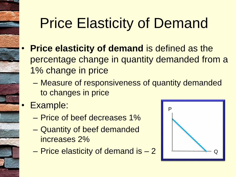
Price Elasticity of Demand
• Price elasticity of demand is defined as the
percentage change in quantity demanded from a
1% change in price
– Measure of responsiveness of quantity demanded
to changes in price
• Example:
– Price of beef decreases 1%
– Quantity of beef demanded
increases 2%
– Price elasticity of demand is – 2
P
Q
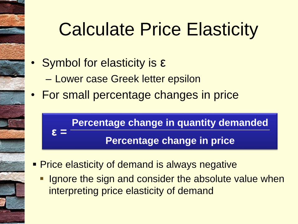
Calculate Price Elasticity
• Symbol for elasticity is ε
– Lower case Greek letter epsilon
• For small percentage changes in price
ε =Percentage change in quantity demanded
Percentage change in price
Price elasticity of demand is always negative
Ignore the sign and consider the absolute value when
interpreting price elasticity of demand

Elastic Demand
• If price elasticity is greater than 1, demand is
elastic
– Percentage change in quantity is greater than
percentage change in price
– Demand is responsive to price
3
Price Elasticity of Demand
Inelastic
Unit elastic
Elastic
210

Inelastic Demand
• If price elasticity is less than 1, demand is
inelastic
– Percentage change in quantity is less than
percentage change in price
– Quantity demanded is not very responsive to price
3
Price Elasticity of Demand
Inelastic
Unit elastic
Elastic
210
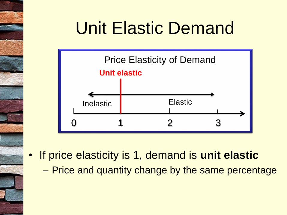
Unit Elastic Demand
• If price elasticity is 1, demand is unit elastic
– Price and quantity change by the same percentage
3
Price Elasticity of Demand
Inelastic
Unit elastic
Elastic
210

Example: Demand for Pizza
Old New % Change
Price $1.00 $0.97 3%
Quantity 400 404 1%
ε =Percentage change in quantity demanded
Percentage change in price
ε =1%
3%= 0.33 Demand is inelastic
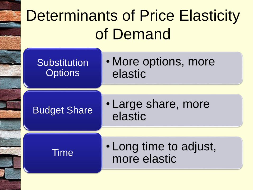
Determinants of Price Elasticity
of Demand
• More options, more elastic
Substitution Options
• Large share, more elastic
Budget Share
• Long time to adjust, more elastic
Time
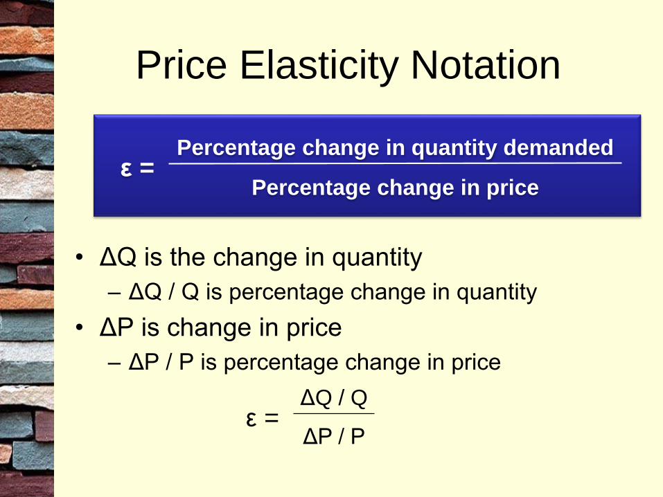
Price Elasticity Notation
• ΔQ is the change in quantity
– ΔQ / Q is percentage change in quantity
• ΔP is change in price
– ΔP / P is percentage change in price
ε =Percentage change in quantity demanded
Percentage change in price
ε =ΔQ / Q
ΔP / P

Price Elasticity: Graphical View
ε =ΔQ / Q
ΔP / P
ε =ΔQ
Q
P
ΔPx
ε =P
Q
ΔQ
ΔPx
ε =P
Q
1
slopex
P – Δ P
Price
P
D
A
Q Q + Δ Q
Δ Q
Δ P
Quantity

Price Elasticity: Graphical View
• At point A
P = 8
Q = 3
Slope = 20 / 5 = 4
ε =8
3
1
4x = 0.67
P – Δ P
Price
P
D
A
Q Q + Δ Q
Δ Q
Δ P
Quantity
ε =P
Q slope
1x

Price Elasticity and Slope
• When two demand curves cross
• P / Q is same for both curves
• (1 / slope) is
smaller for the
steeper curve
– At the common
point demand
is less price elastic
for the steeper
curve
D1
D2
12
4 6 12
6
4
Quantity
Price
Less Elastic
More Elastic
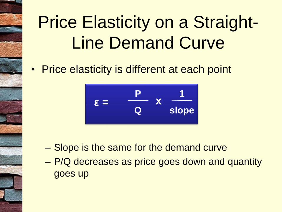
Price Elasticity on a Straight-
Line Demand Curve
• Price elasticity is different at each point
– Slope is the same for the demand curve
– P/Q decreases as price goes down and quantity
goes up
ε =P
Q
1
slopex

Price Elasticity Pattern
• Price elasticity changes systematically as price goes
down
• At high P and low Q, P / Q is large
• Demand is elastic
• At the midpoint,
demand is unit elastic
• At low P and high Q,
P / Q is small
• Demand is
inelastic
Price
b/2
a/2
a
b
1
1
1
Quantity

Two Special Cases
Perfectly Elastic
Demand
• Infinite price elasticity of
demand
Perfectly Inelastic
Demand
• Zero price elasticity of
demand
Price
Quantity
D
Price
Quantity
D
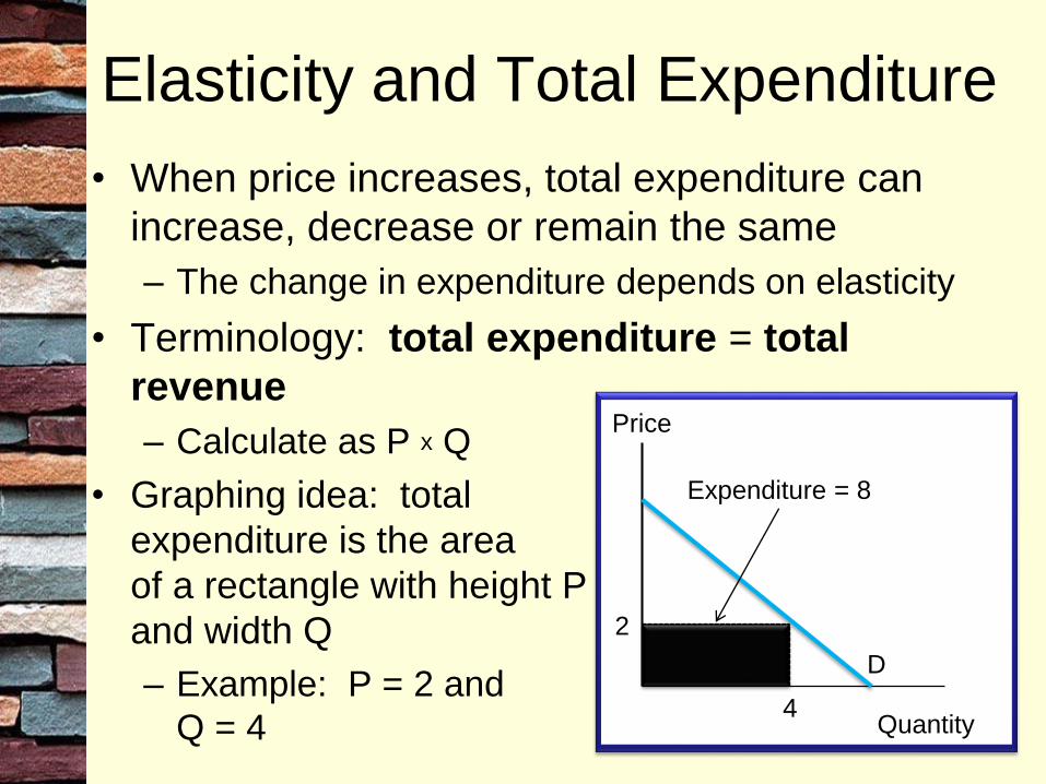
Elasticity and Total Expenditure
• When price increases, total expenditure can
increase, decrease or remain the same
– The change in expenditure depends on elasticity
• Terminology: total expenditure = total
revenue
– Calculate as P x Q
• Graphing idea: total
expenditure is the area
of a rectangle with height P
and width Q
– Example: P = 2 and
Q = 4
Price
Quantity
D
2
4
Expenditure = 8

Price Elasticity and Total
Expenditure• Movie ticket price increases from $2 to $4
– A and B are both below the midpoint of the curve
• Inelastic portion of the demand curve
– Total revenue increases when price increases
Quantity (00s of tickets/day)
D
A
Expenditure =
$1,000/day
12
Price (
$/t
icket)
5 6
2
Quantity (00s of tickets/day)
4
D
B
Expenditure =
$1,600/day
12
Price (
$/t
icket)
6
4
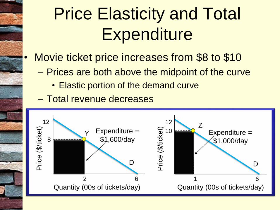
Price Elasticity and Total
Expenditure
• Movie ticket price increases from $8 to $10
– Prices are both above the midpoint of the curve
• Elastic portion of the demand curve
– Total revenue decreases
D
Expenditure =
$1,600/day
12
Quantity (00s of tickets/day)
Price (
$/t
icket)
2 6
8Y
Z
D
Expenditure =
$1,000/day
12
Quantity (00s of tickets/day)
Price (
$/t
icket)
1 6
10
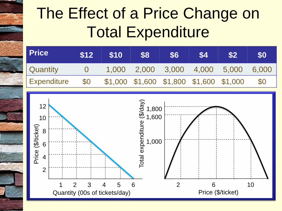
The Effect of a Price Change on
Total ExpenditurePrice $12 $10 $8 $6 $4 $2 $0
Quantity 0 1,000 2,000 3,000 4,000 5,000 6,000
Expenditure $0 $1,000 $1,600 $1,800 $1,600 $1,000 $0
1,800
Price ($/ticket)
Tota
l expenditure
($/d
ay)
2 6 10
1,600
1,000
12
Quantity (00s of tickets/day)
Pri
ce
($
/tic
ke
t)
1 3 4 5 6
10
8
6
4
2
2
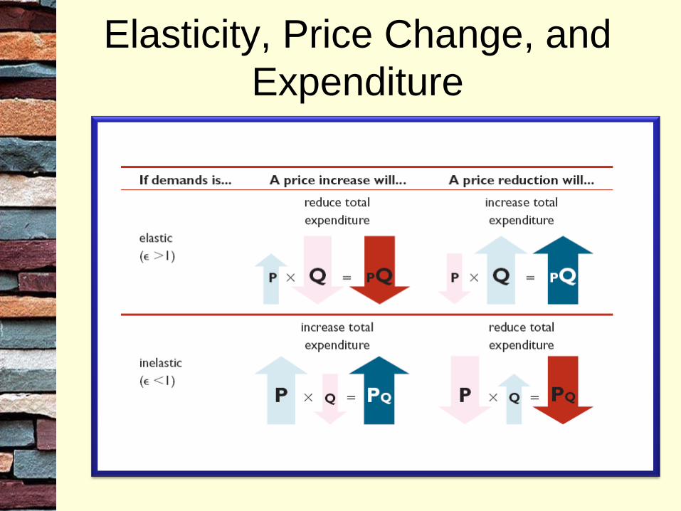
Elasticity, Price Change, and
Expenditure

Cross-Price Elasticity of Demand
• Substitutes and complements affect demand
• Cross-price elasticity of demand is defined
as the percentage change in quantity
demanded of good A from a 1 percent change
in the price of good B
• Sign of cross-price elasticity shows
relationship between the goods
– Complements have negative cross-price elasticity
– Substitutes have positive cross-price elasticity
– Do not ignore the sign when interpreting corss-
price elasticity of demand
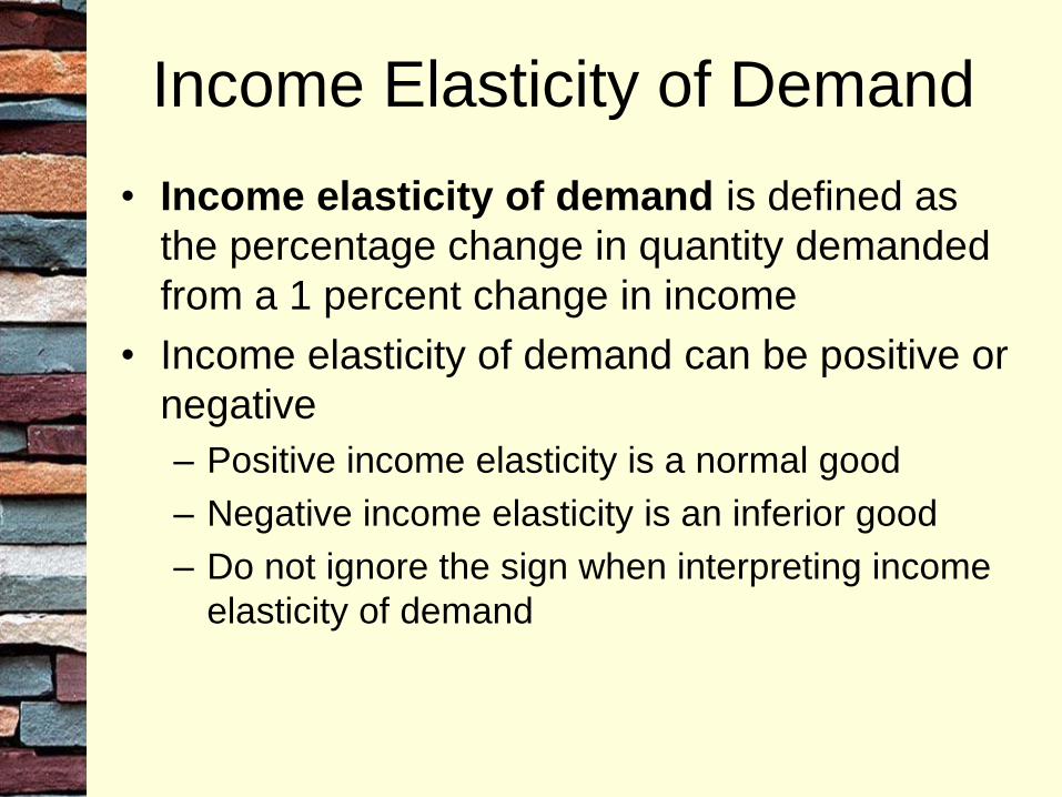
Income Elasticity of Demand
• Income elasticity of demand is defined as
the percentage change in quantity demanded
from a 1 percent change in income
• Income elasticity of demand can be positive or
negative
– Positive income elasticity is a normal good
– Negative income elasticity is an inferior good
– Do not ignore the sign when interpreting income
elasticity of demand

Calculate Income and Cross-
Price Elasticity• Income elasticity of demand:
• Cross-price elasticity of demand:
εI =Percentage change in quantity demanded
Percentage change in Income
εAB =Percentage change in quantity demanded of A
Percentage change in Price of B
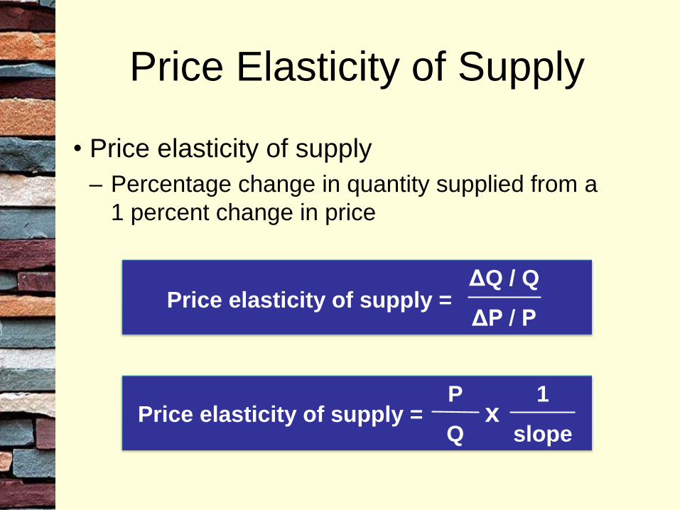
Price Elasticity of Supply
• Price elasticity of supply
– Percentage change in quantity supplied from a
1 percent change in price
Price elasticity of supply =ΔQ / Q
ΔP / P
Price elasticity of supply =P
Q
1
slopex
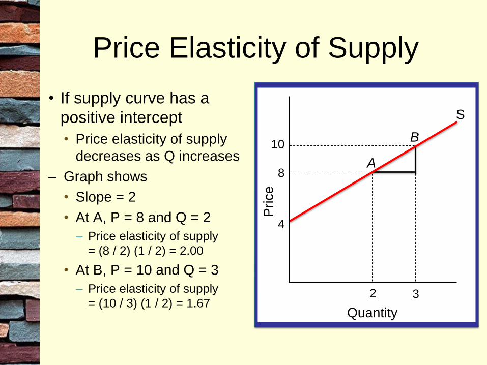
Price Elasticity of Supply
• If supply curve has a
positive intercept
• Price elasticity of supply
decreases as Q increases
– Graph shows
• Slope = 2
• At A, P = 8 and Q = 2
– Price elasticity of supply
= (8 / 2) (1 / 2) = 2.00
• At B, P = 10 and Q = 3
– Price elasticity of supply
= (10 / 3) (1 / 2) = 1.672
8A
3
10B
Quantity
Price
4
S

Price Elasticity of Supply
• If supply curve has a zero
intercept
• Price elasticity of supply is
1.00
– Graph shows
• Slope = 1 / 3
• At A, P = 4 and Q = 12
– Price elasticity of supply
= (4 / 12) (3) = 1.00
• At B, P = 5 and Q = 15
– Price elasticity of supply
= (5 / 15) (3) = 1.00 15
5B
ΔP
Δ Q
S
12
4A
Quantity
Price

Perfectly Inelastic Supply
• Zero price elasticity of
supply
• No response to
change in price
• Example: land in
Tokyo
• Supply is completely
fixed
• Any one-of-a-kind
item has perfectly
inelastic supply
• Work of art (Mona
Lisa)
• Hope Diamond
Price
Quantity
S
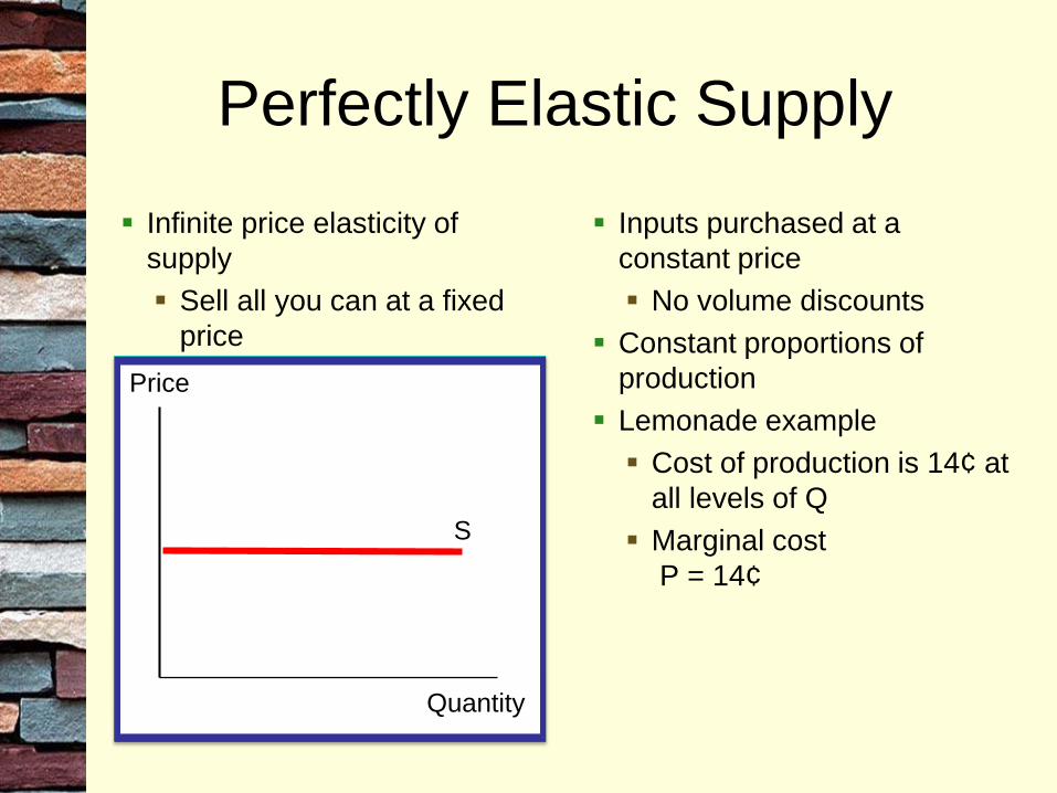
Perfectly Elastic Supply
Infinite price elasticity of
supply
Sell all you can at a fixed
price
Inputs purchased at a
constant price
No volume discounts
Constant proportions of
production
Lemonade example
Cost of production is 14¢ at
all levels of Q
Marginal cost
P = 14¢
Price
Quantity
S

Determinants of Price Elasticity
of Supply
• Uses adaptable inputs, more elastic
Input Flexibility
• Resources move where needed, more elastic
Mobility of Inputs
• Alternative inputs easy to find, more elastic
Produce Substitute Inputs
• Long run, more elasticTime
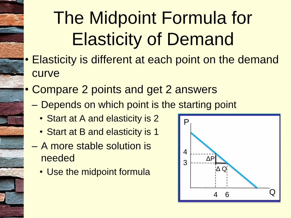
• Elasticity is different at each point on the demand
curve
• Compare 2 points and get 2 answers
– Depends on which point is the starting point
• Start at A and elasticity is 2
• Start at B and elasticity is 1
– A more stable solution is
needed
• Use the midpoint formula
The Midpoint Formula for
Elasticity of Demand
P
Q
ΔP
Δ Q
4
3
4 6

The Midpoint Formula for
Elasticity of Demand
• Midpoint formula
– Use average quantity in the numerator
– Use average price in the denominator
• Elasticity using midpoint
formula is 1.40
ΔQ / [(QA + QB)/2]
Δ P / [(PA + PB)/2]ε =
Δ Q / (QA + QB)
Δ P / (PA + PB)ε =
P
Q
ΔP
Δ Q
4
3
4 6

Needs versus Wants
• Some goods are required for subsistence
– These are needs
• Beyond subsistence, behavior is driven by wants
– Rice or noodle
– Hamburger or chicken sandwich
• Wants depend on price
• Unlimited wants with limited resources means
consumers have to prioritize wants when making
choices.

Wants and Utility
• Utility: the satisfaction people derive from
consumption
– Well-being, happiness
– Measured indirectly
• Subjective
• Observable
– Cannot be compared between people
• Individual goal is to maximize utility
– Allocate resources accordingly
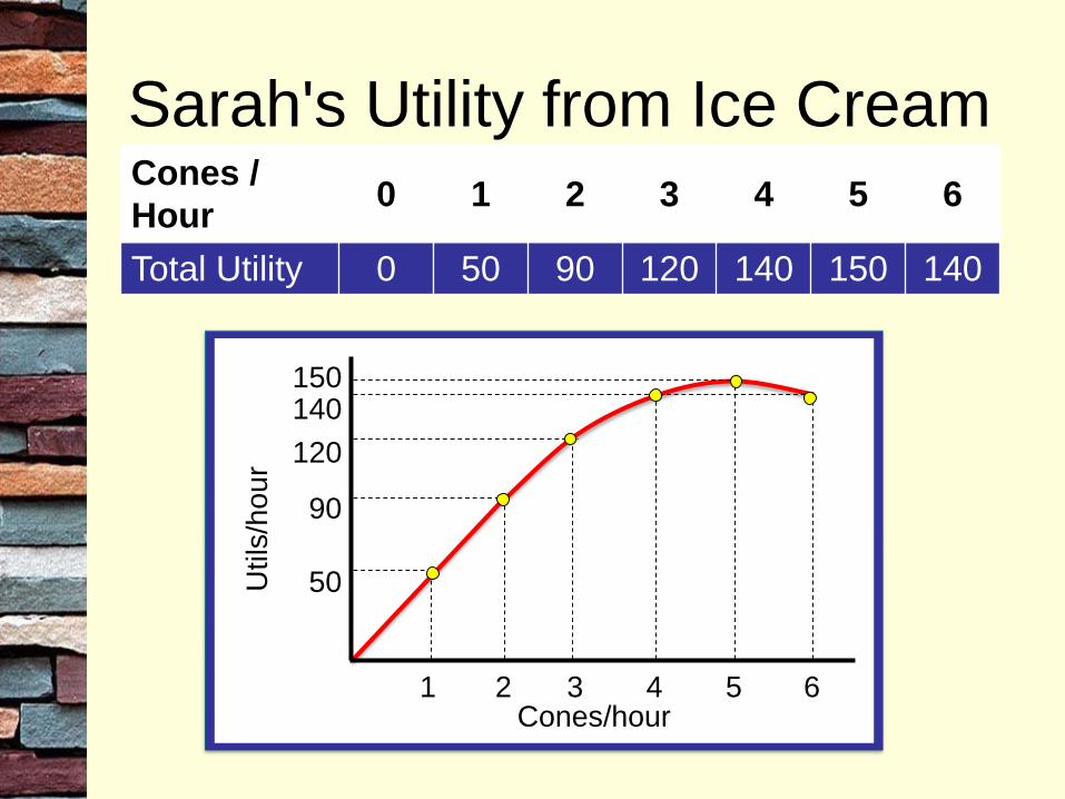
Sarah's Utility from Ice CreamCones /
Hour0 1 2 3 4 5 6
Total Utility 0 50 90 120 140 150 140
Cones/hour
Utils
/hou
r
1 3 4 5 62
150140
120
90
50

Sarah's Marginal Utility from Ice
Cream
• Marginal utility: the additional utility from
consuming one more
Cones /
Hour0 1 2 3 4 5 6
Total Utility 0 50 90 120 140 150 140
Marginal Utility 50 40 30 20 10 -10
Marginal utility = Change in utility
Change in consumption
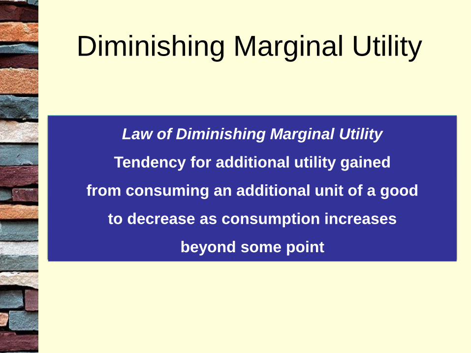
Law of Diminishing Marginal Utility
Tendency for additional utility gained
from consuming an additional unit of a good
to decrease as consumption increases
beyond some point
Diminishing Marginal Utility

Diminishing Marginal Utility
• Marginal utility can increase at low levels of
consumption
– First unit stimulates your desire for more
• First unit of food/drinks
• Eventually marginal utility declines
– Continue consuming
• Apply Cost-Benefit Principle
– Consume an additional unit as long as the marginal
utility (benefit) is greater than the marginal cost

Spending on Two Goods
• Assume a fixed budget
• Decide how much of each
good to buy
• Law of Diminishing
Marginal Utility applies
– As you buy more of a single
good, its marginal utility
decreases
– When you buy less of that
good, its marginal utility
increases
Ma
rgin
al U
tilit
y
Ma
rgin
al U
tility
Budget Allocation
• Maximize utility when the marginal utility per
dollar spent is the same for all goods
• No Money Left On the Table Principle
– Current spending has marginal utility of a dollar spent
on one good higher than the marginal utility of a
dollar spent on the other good
– Take a dollar away from the good with low marginal
utility and spend it on the good with high marginal
utility
• Marginal utilities per dollar begin to equalize

Sarah's Ice Cream
• $400 budget
• Chocolate is $2 per pint
• Vanilla is $1 per pint
• Buy 200 pints of vanilla
and 100 pints of
chocolate
• Marginal utility is 12 for
vanilla, 16 for chocolate
Pints/yr
Vanilla
Ice Cream
12
200
MU
(u
tils
/ pin
t)
Chocolate
Ice Cream
Pints/yr
16
100
MU
(u
tils
/ pin
t)
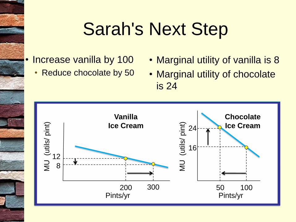
Sarah's Next Step
• Increase vanilla by 100
• Reduce chocolate by 50
• Marginal utility of vanilla is 8
• Marginal utility of chocolate
is 24
Chocolate
Ice Cream
Pints/yr
16
100M
U (u
tils
/ pin
t)50
24
Pints/yr
Vanilla
Ice Cream
200
MU
(u
tils
/ pin
t)
300
8
12

Sarah's Equilibrium
• Optimal combination:
highest total utility
• 250 pints vanilla; 75 pints
chocolate
• Marginal utility / price is
the same for all goods
• Marginal utility of vanilla
10, chocolate 20
MU
(u
tils
/ pin
t)
Pints/yr
Vanilla
Ice Cream
250
10
MU
(u
tils
/ pin
t)
Chocolate
Ice Cream
Pints/yr
20
75

Sarah's ChoicesScenario
1Price Quantity
Marginal
Utility MU / $
Vanilla $1 200 12 12
Chocolate $2 100 16 8
Scenario
2Price Quantity
Marginal
Utility MU / $
Vanilla $1 300 8 8
Chocolate $2 50 24 12
Scenario
3Price Quantity
Marginal
Utility MU / $
Vanilla $1 250 10 10
Chocolate $2 75 20 10

The Rational Spending Rule
Spending should be allocated across goods so that
the marginal utility per dollar
is the same for each good
Rational Spending Rule

Rational Spending Rule• Rational Spending Rule can be written
algebraically
• Notation
– MUC is the marginal utility from chocolate
– MUV is the marginal utility from vanilla
– PC is the price of chocolate
– PV is the price of vanilla
• Rational Spending Rule
MUC / PC = MUV / PV
• The marginal utility per dollar spent on chocolate
equals the marginal utility per dollar spent on
vanilla
Substitution Effect
• When the price of a good goes up, substitutes for
that good are relatively more attractive
– At the higher price less is demanded because some
buyers switch to the substitute good
– If the price of vanilla ice cream goes up, some buyers
will buy less vanilla and more chocolate

Income Effect
• Changes in price affect the buyers' purchasing
power
– Acts like a change in income
• Suppose vanilla ice cream goes from $1 per pint
to $2
– If Sarah spends all her income on vanilla, the amount
she can buy goes down by half
– At the original prices, she could buy 100 pints of
vanilla and 150 pints of chocolate
• At new price for vanilla, she buys 100 vanilla and only
100 chocolate

Rational Spending and Price
Changes• Suppose price of vanilla increases from $1 to $2
• At the original equilibrium
MUC / PC = MUV / PV
• With the increase in PV, MUV / PV < MUC / PC
– If Sarah buys more chocolate, MUC will go down
– If Sarah buys less vanilla, MUV will go up
– To get to a new optimal spending point,
• Buy more chocolate
• Buy less vanilla
• Stop when the marginal utility per dollar is the same
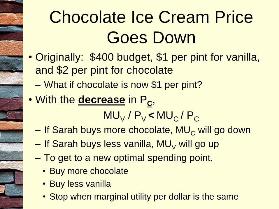
Chocolate Ice Cream Price
Goes Down• Originally: $400 budget, $1 per pint for vanilla,
and $2 per pint for chocolate
– What if chocolate is now $1 per pint?
• With the decrease in PC,
MUV / PV < MUC / PC
– If Sarah buys more chocolate, MUC will go down
– If Sarah buys less vanilla, MUV will go up
– To get to a new optimal spending point,
• Buy more chocolate
• Buy less vanilla
• Stop when marginal utility per dollar is the same

Market and Social Welfare
• Market is the aggregation of individual consumer
demand and producer supply
• Consumers and producers are able to acquire
welfare from consumption and production of
products in the market
• Welfare of the society (Economic surplus) is
obtained by the sum of the consumers and
producers welfare
• Economic surplus = Consumer surplus +
producer surplus

Individual and Market Demand
Curves• The market demand is the horizontal sum of
individual demand curves
– At each possible price, add up the number of units
demanded by individuals to get the market demand
Smith Jones Market

Consumer Surplus
• Consumer surplus is the difference between
the buyer's reservation price and the market
price
• With multiple buyers
– Find the consumer surplus for each buyer
– Add up the individual surplus for each buyer
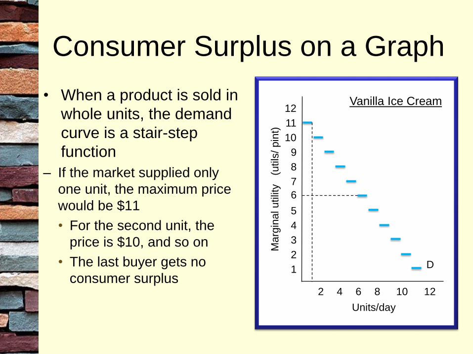
Consumer Surplus on a Graph
• When a product is sold in
whole units, the demand
curve is a stair-step
function
– If the market supplied only
one unit, the maximum price
would be $11
• For the second unit, the
price is $10, and so on
• The last buyer gets no
consumer surplusD
Units/day
Marg
inal utilit
y
(utils
/ pin
t)1
2
3
4
5
6
7
8
9
10
11
12
2 4 6 8 10 12
Vanilla Ice Cream
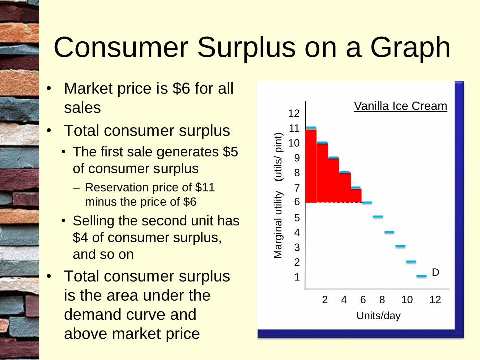
Consumer Surplus on a Graph
• Market price is $6 for all
sales
• Total consumer surplus
• The first sale generates $5
of consumer surplus
– Reservation price of $11
minus the price of $6
• Selling the second unit has
$4 of consumer surplus,
and so on
• Total consumer surplus
is the area under the
demand curve and
above market price
D
Units/day
Marg
inal utilit
y
(utils
/ pin
t)1
2
3
4
5
6
7
8
9
10
11
12
2 4 6 8 10 12
Vanilla Ice Cream
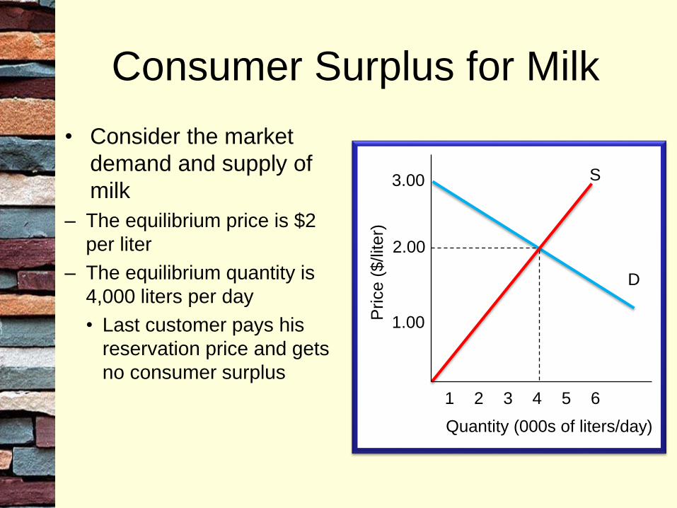
Consumer Surplus for Milk
• Consider the market
demand and supply of
milk
– The equilibrium price is $2
per liter
– The equilibrium quantity is
4,000 liters per day
• Last customer pays his
reservation price and gets
no consumer surplus
Quantity (000s of liters/day)
Price (
$/liter)
1
1.00
2.00
3.00
2 3 4 5 6
S
D

Consumer Surplus for Milk
• Price is $2 and quantity
is 4,000 liters per day
• Consumer surplus is the
area of the triangle
between:
• Horizontal intercept of
demand
• Market price
• Market quantity
– Remember: area of a right
triangle is ½ base times
height
• The area is
½ (4,000 liter)($1) = $2,000
Quantity (000s of liter/day)
Price (
$/liter)
1
1.00
2.00
3.00
2 3 4 5 6
S
D
Consumer
Surplus
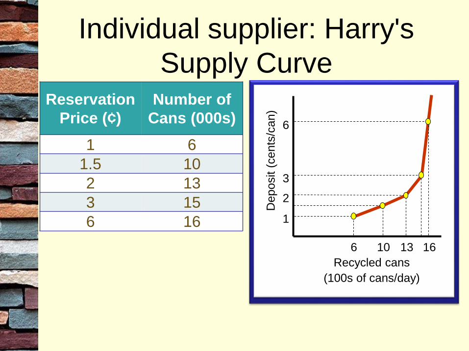
Individual supplier: Harry's
Supply CurveReservation
Price (¢)
Number of
Cans (000s)
1 6
1.5 10
2 13
3 15
6 16
Recycled cans
(100s of cans/day)D
eposit (
cents
/can)
6 10 13 16
6
3
2
1
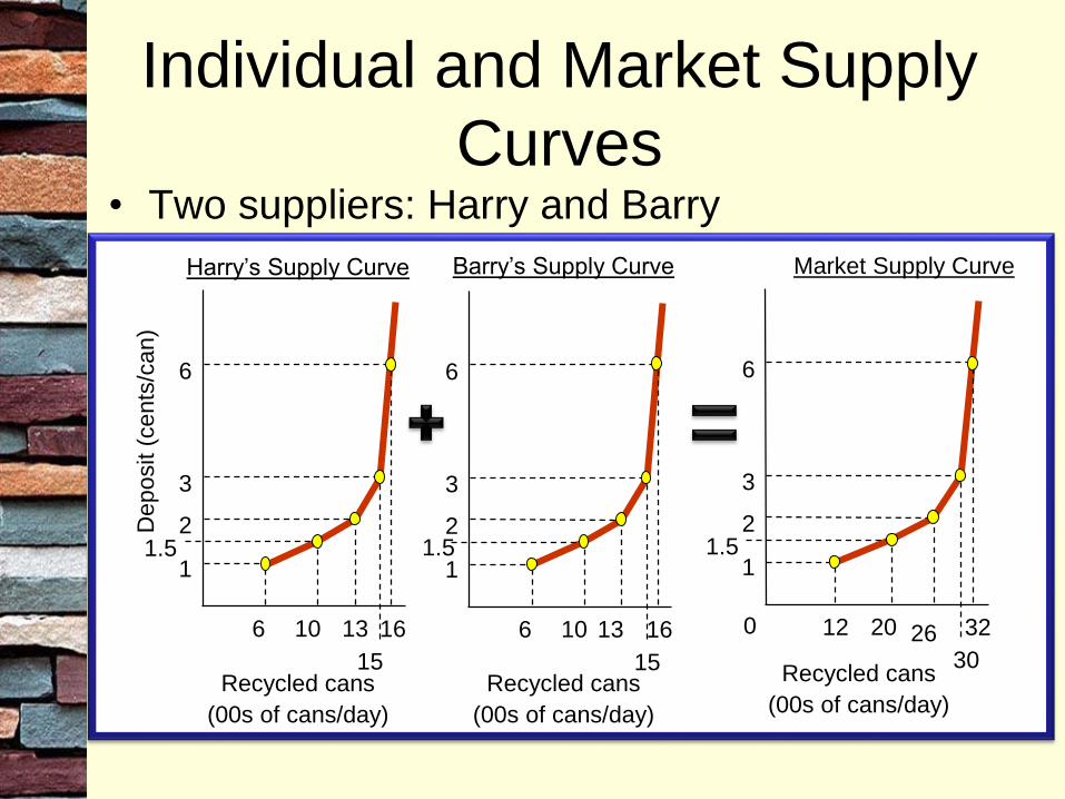
Individual and Market Supply
Curves• Two suppliers: Harry and Barry
Recycled cans
(00s of cans/day)
Deposit (
cents
/can)
Harry’s Supply Curve
Recycled cans
(00s of cans/day)
Barry’s Supply Curve
Recycled cans
(00s of cans/day)
016
6
16
6
32
6
6
1
6
1
12
1
10
1.5 1.5
10 20
1.5
13
3
2
15
13
3
2
15
26
3
2
30
Market Supply Curve

Producer Surplus• Producer surplus is the difference between the
market price and the seller's reservation price
• Reservation price = Marginal cost which is on the
supply curve
• Producer surplus is the area above the supply
curve and below the market price
Related Documents


![C5.2 Elasticity and Plasticity [1cm] Lecture 2 Equations ...](https://static.cupdf.com/doc/110x72/622f8f3994946046a5727b7b/c52-elasticity-and-plasticity-1cm-lecture-2-equations-.jpg)