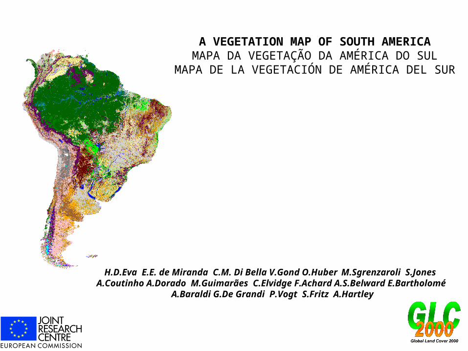
H.D.Eva E.E. de Miranda C.M. Di Bella V.Gond O.Huber M.Sgrenzaroli S.Jones A.Coutinho A.Dorado M.Guimarães C.Elvidge F.Achard A.S.Belward E.Bartholomé.

H.D.Eva E.E. de Miranda C.M. Di Bella V.Gond O.Huber M.Sgrenzaroli S.Jones A.Coutinho A.Dorado M.Guimarães C.Elvidge F.Achard A.S.Belward E.Bartholomé

A.Baraldi G.De Grandi P.Vogt S.Fritz A.Hartley

A VEGETATION MAP OF SOUTH AMERICAMAPA DA VEGETAÇÃO DA AMÉRICA DO SUL

MAPA DE LA VEGETACIÓN DE AMÉRICA DEL SUR

Contributing Institutions

Venezuela

Southern Cone

Amazon forest

Regional Experts working on data

Brazil

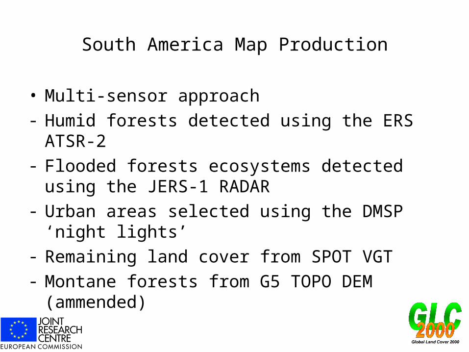
South America Map Production

• Multi-sensor approach- Humid forests detected using the ERS ATSR-2- Flooded forests ecosystems detected using the JERS-

1 RADAR- Urban areas selected using the DMSP ‘night lights’- Remaining land cover from SPOT VGT- Montane forests from G5 TOPO DEM (ammended)

Humid forests detected using the ERS ATSR-2

-Over 1000 images to create a mosaic based on highest surface temperature – “tropical dry season”

-Unsupervised spectral clustering

-Class labeling for humid forests and non-forests

ATSR-2

1 km resolution: 500 km swath: Green / Red / NIR / SWIR and TIR channels

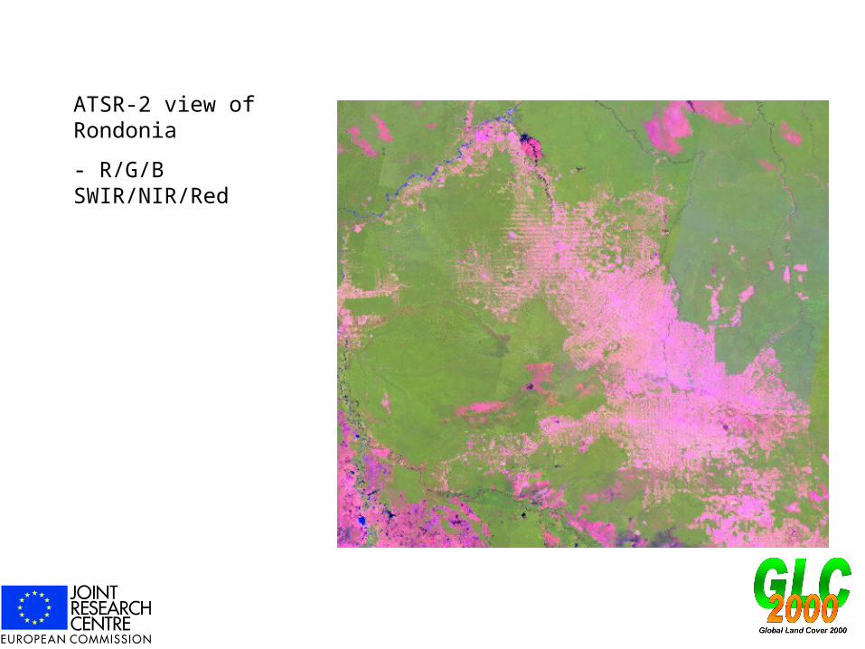
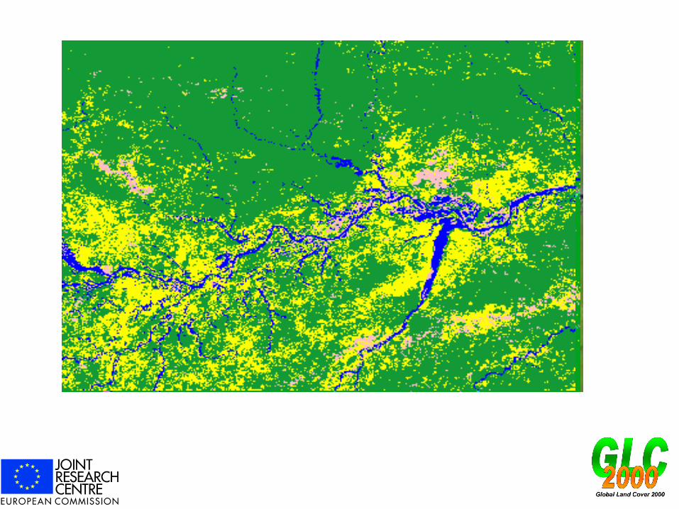
ATSR-2 view of Rondonia

- R/G/B SWIR/NIR/Red

JERS-1 RADAR for flooded forests

- Two JERS-1 Mosaics – high water and low water

-Radar backscatter is increased by the the ‘double bounce’ off water and trees – high backscatter shows flooded forests

-The difference between the two images shows up seasonally flooded areas

Land cover from the SPOT VGT data

-Preparation of ‘seasonal’ mosaics from S10 data

-‘Winter’ ‘Spring’ ‘Summer’ ‘Autumn’ – selected on lowest SWIR (thresholded)

-Composited to the full year (Red NIR and SWIR)

-Humid forests (ATSR) mask

-Unsupervised classification 60 classes to remaining area

-Class labeling

-Extraction of particular areas from seasonal mosaics (e.g. removal of Snow)

Creation of seasonal mosaics from S10 product

Jan-Mar Apr-Jun July-Sept Oct-Dec

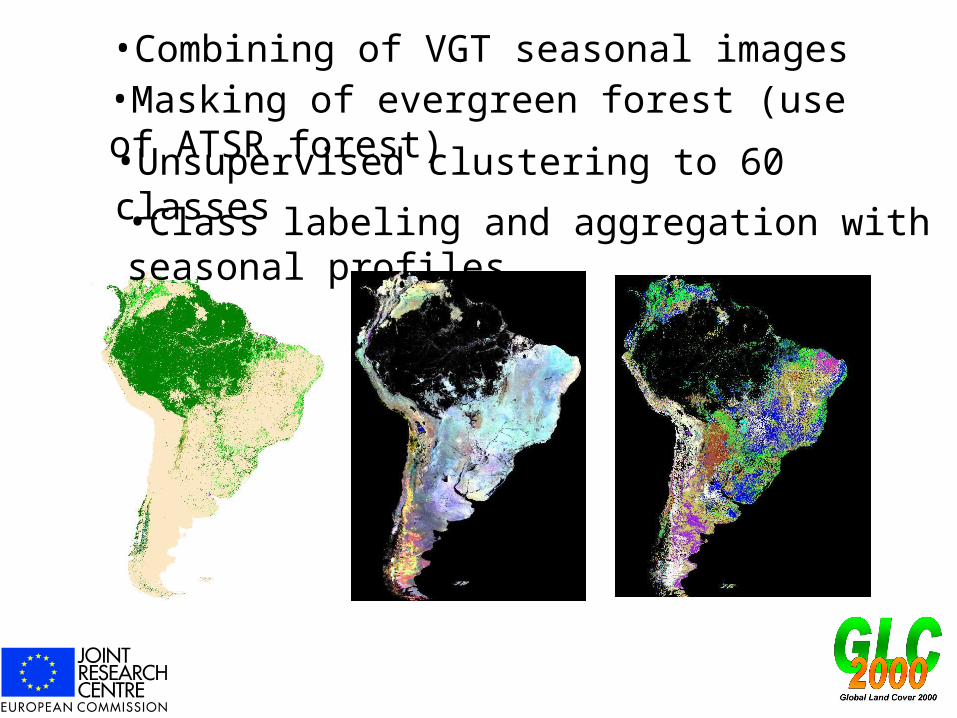
•Combining of VGT seasonal images•Masking of evergreen forest (use of ATSR forest)

•Unsupervised clustering to 60 classes

•Class labeling and aggregation with seasonal profiles

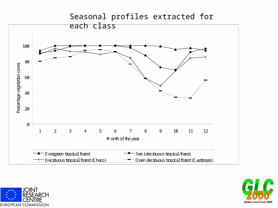
0

20

40

60

80

100

1 2 3 4 5 6 7 8 9 10 11 12

Month of the year

Per

cent

age

vege

tati

on c

over

Evergreen tropical forest Semi deciduous tropical forest

Deciduous tropical forest (Chaco) Open deciduous tropical forest (Caatingas)

Seasonal profiles extracted for each class

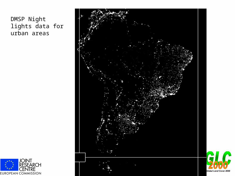
DMSP Night lights data for urban areas

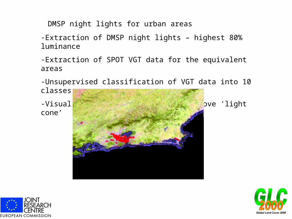
DMSP night lights for urban areas

-Extraction of DMSP night lights – highest 80% luminance

-Extraction of SPOT VGT data for the equivalent areas

-Unsupervised classification of VGT data into 10 classes

-Visual examination of classes to remove ‘light cone’

Validation data

TREES High resolution data set – 40 scenes spread across the humid forest domain

Advantages – cost, availability, expert interpretation

Disadvantages – a bias in selection and in classification scheme used (i.e. for forest change), data are from 1997, fragmented classes

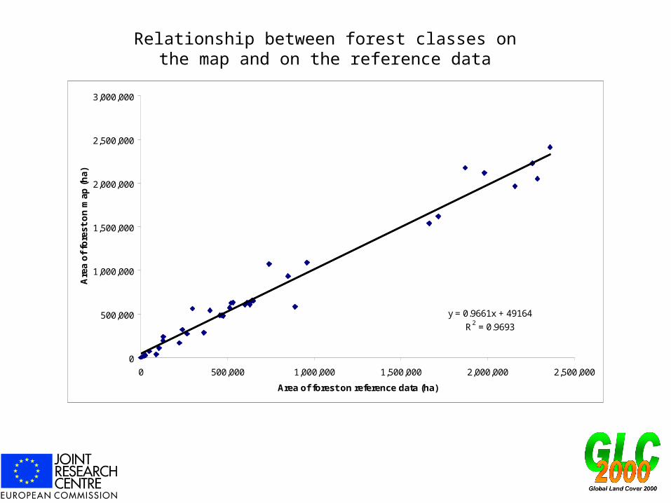
y = 0.9661x + 49164

R2 = 0.9693

0

500,000

1,000,000

1,500,000

2,000,000

2,500,000

3,000,000

0 500,000 1,000,000 1,500,000 2,000,000 2,500,000

Area of forest on reference data (ha)

Are

a o

f fo

rest

on

map

(h

a)

Relationship between forest classes on the map and on the reference data

Forests Shrublands Grasslands Sparse grasslands Agriculture Mosaic 1 Mosaic 2 Bare Urban WaterReference data Forest 83% 17% 13% 7% 17% 39% 14% 6% 0% 11%Woodland &Shrubland 3% 17% 7% 19% 5% 5% 21% 5% 1% 1%Grassland 3% 40% 60% 25% 2% 1% 25% 11% 3% 5%Agriculture 6% 9% 8% 9% 57% 35% 29% 2% 19% 2%Bare 0% 5% 4% 34% 1% 0% 4% 72% 68% 2%Mosaic 4% 11% 5% 6% 18% 21% 7% 1% 3% 1%Water 1% 1% 4% 0% 0% 0% 0% 2% 6% 78%

100% 100% 100% 100% 100% 100% 100% 100% 100% 100%

Map data

Forest class: 83% forest

Mosaic 1 (agriculture and degraded forest): 39% forest 35 % agriculture 21 % mosaics (agriculture and other)

Mosaic 2 (agriculture and other vegetation): 21% woodland/shrubland 25% grassland 29% agriculture

Agriculture : 57% agriculture 18% mosaic (agriculture and other)

A brake-down of map classes by reference classes

Conclusions

•Map is a result of a network of experts and institutions

•Final data product is available at the regional level and can be aggregated to different general levels

•Data have undergone a first level validation

•Data have been provided on the Web and downloaded by over 120 different institutions

•Thanks to regional experts and to GIS support