JavaHAWKS (JAVA HITRAN ATMOSPHERIC WORKSTATION) MANUAL For MS Windows, UNIX, LINUX, and MAC Operating Systems Laurence S. Rothman Atomic and Molecular Physics Division Harvard-Smithsonian Center for Astrophysics 60 Garden St, Cambridge MA 02138-1516 John Schroeder and Kuilian Tang Ontar Corporation 9 Village Way, North Andover MA 01845-2000 USA September 2004

Welcome message from author
This document is posted to help you gain knowledge. Please leave a comment to let me know what you think about it! Share it to your friends and learn new things together.
Transcript
JavaHAWKS (JAVA HITRAN ATMOSPHERIC WORKSTATION)
MANUAL
For MS Windows, UNIX, LINUX, and MAC Operating Systems
Laurence S. Rothman Atomic and Molecular Physics Division
Harvard-Smithsonian Center for Astrophysics 60 Garden St, Cambridge MA 02138-1516
John Schroeder and Kuilian Tang Ontar Corporation
9 Village Way, North Andover MA 01845-2000 USA
September 2004

JavaHAWKS Manual
JavaHAWKS Manual
i
1. SOFTWARE INSTALLATION........................................................................................................1 1.1. INSTALLATION FILES.......................................................................................................................1 1.2. INSTALLATION PROCEDURES...........................................................................................................1 1.3. LAUNCHING THE JAVAHAWKS APPLICATION ................................................................................2
2. HITRAN AND JAVAHAWKS..........................................................................................................3
3. INITIATING THE OPERATION OF JAVAHAWKS...................................................................6 3.1. FILE OPTION....................................................................................................................................7
3.1.1. Change Format .......................................................................................................................7 3.1.2. Exit ..........................................................................................................................................8
3.2. SELECT OPTION...............................................................................................................................8 3.2.1. HITRAN Filename ..................................................................................................................9 3.2.2. Output Filename .....................................................................................................................9 3.2.3. Spectral Range ......................................................................................................................10 3.2.4. Molecule................................................................................................................................10 3.2.5. Isotopologue..........................................................................................................................11 3.2.6. Temperature..........................................................................................................................12 3.2.7. Band ......................................................................................................................................12 3.2.8. Cutoff.....................................................................................................................................14 3.2.9. RUN SELECT........................................................................................................................14 3.2.10. RUN DESELECT ................................................................................................................15
3.3. BAND STATS OPTION ....................................................................................................................15 3.4. SORT OPTION ................................................................................................................................17
3.4.1. Sort........................................................................................................................................17 3.4.2. Merge ....................................................................................................................................18
3.5. INTERNET OPTION .........................................................................................................................19 3.5.1 HITRAN Website....................................................................................................................19 3.5.2 HITRAN FTP Site ..................................................................................................................19 3.5.3 JPL Submillimeter Data.........................................................................................................19 3.5.4 Cologne Spectroscopy Data...................................................................................................20 3.5.5 CfA UV Xsection Data ...........................................................................................................21
3.6. REFERENCE OPTION ......................................................................................................................21 3.6.1. Molecule................................................................................................................................22 3.6.2. Wavenumber .........................................................................................................................22 3.6.3. Xsection.................................................................................................................................22
3.7. PLOT OPTION.................................................................................................................................22 3.7.1 Difference Plot ......................................................................................................................25 3.7.2. Plotting Cross-Section Data .................................................................................................26 3.7.3. Edit Plot and Print Plot ........................................................................................................27
3.8. HELP OPTION ................................................................................................................................28 3.8.1. About .....................................................................................................................................28
4. ACKNOWLEDGMENTS ................................................................................................................28
5. REFERENCES..................................................................................................................................29
APPENDIX A. DIRECTORIES AND FILES IN HITRAN (V11.0)................................................30
APPENDIX B. HITRAN (V11.0) MOLECULES WITH ASSOCIATED INDICES .....................32
JavaHAWKS Manual
ii
APPENDIX C. SCHEMATIC OF FUNDAMENTAL SPECTROSCOPIC PARAMETERS OF A LINE TRANSITION IN HITRAN. ..................................................................................................... 33
APPENDIX D. FORMATS FOR LINE-BY-LINE PARAMETERS AND CROSS-SECTION HEADERS.............................................................................................................................................. 34
JavaHAWKS Manual
1
This manual is designed to assist the user in easily adapting to the manipulation of the HITRAN (High
Resolution Transmission) molecular spectroscopic database and associated molecular databases by
proper utilization of the JavaHAWKS software package.
1. Software Installation
The software has been written in the Java language so that we can maintain cross-platform
performance, and at the same time maintain a single source code. In order to install and run the
software, you must have a version of the Java runtime environment running on your computer. Java is
common on most UNIX computers and many PC and MAC network systems. The installation program
will search your computer for Java and will not complete the installation unless a suitable version of
Java is installed on your computer. If this is the case, you are advised to consult your system
administrator or other computer maintenance personnel about having Java installed on your computer.
We cannot be responsible for assisting you in this task, since most systems administrators have
specific requirements that must be met.
1.1. Installation Files
All installation files for different platforms are distributed via the HITRAN ftp-site
(ftp://cfa-ftp.harvard.edu/pub/HITRAN/). These files are: (1) Win_Setup.exe; (2) Linux_Setup.bin; (3)
Unix_Setup.bin; (4) MacOS_Setup.bin; (5) MacOSX_Setup.zip and (6) Software-Readme. The first
five files are JavaHAWKS installers for different operating systems. The file “Installer of
JavaHAWKS for Windows.exe” is for the PC, Linux_Setup is for Linux, Unix_Setup.bin is for any
generic Unix system (e.g. Solaris, Linux, Unix, etc), MacOS_Setup.bin is for any Macintosh with
operating system from 8.x to 9.x, and MacOSX_Setup.zip is for Macintosh with OS X operating
system. Based on the platform one is using, a proper installer should be downloaded from the
HITRAN ftp-site. Compared to previous installations of JavaHAWKS, these new installers will greatly
simplify the procedures of installing JavaHAWKS on the user’s computer, especially for Macintosh
users. The Software-Readme file gives the user details about the installation of JavaHAWKS on
different platforms and how the user launches the application, which is described below.
1.2. Installation Procedures
Please refer to the introductory paragraph in section 1 about having the Java runtime environment

JavaHAWKS Manual
2
installed on your computer before proceeding with the installation. It is the user’s responsibility to
decide which installation file he/she should download from the HITRAN ftp-site based on the platform
he/she is using. Please refer to section 1.1 to decide which installer to download. Description of the
installation procedures is given below for each of different platforms respectively.
PC Windows
1. Download the installation file “Installer of JavaHAWKS for Windows.exe” from the HITRAN
FTP site.
2. Double click the downloaded file to launch the JavaHAWKS installation wizard.
3. Follow the installation procedures step-by-step until finally clicking the “Done” button.
Generic Unix/Linux
1. Download the installation file Unix_Setup.bin or Linux_Setup.bin from the HITRAN ftp-site to a
temporary location.
2. Go to the temporary location from the shell.
3. Type in sh Unix_Setup.bin or sh Linux_Setup.bin from the command line and hit return. The
JavaHAWKS installation wizard will appear.
4. Follow the installation procedures step-by-step until finally clicking the “Done” button.
Macintosh OS 8.0-9.x
1. Download the installation file MacOS_Setup.bin from the HITRAN ftp-site to a temporary
location or to desktop.
2. Double click the downloaded file and a file called installer.bin will be created.
3. Double click the file installer.bin to launch the JavaHAWKS installation wizard.
4. Follow the installation procedures step-by-step until finally clicking the “Done” button.
Macintosh OS X
1. Download the installation file MacOSX_Setup.zip from the HITRAN ftp-site to a temporary
location or to desktop.
2. Double click the downloaded file and a file called installer.bin will be created.
3. Double click the file installer.bin to launch the JavaHAWKS installation wizard.
4. Follow the installation procedures step-by-step until finally clicking the “Done” button.
1.3. Launching the JavaHAWKS application
Depending on the platform the user is employing, the way to launch the JavaHAWKS application may
JavaHAWKS Manual
3
be different. It also depends on how the user chooses to create the application icon during the
installation. Following is a general description about how to launch the application for each different
platform respectively.
PC Windows
The alternative ways to launch the JavaHAWKS application include the following.
1. If you choose to create an icon on the desktop during the installation, double clicking on the
JavaHAWKS icon on the desktop will launch the application.
2. If you choose to create an icon in the Start menu during the installation, click the Start menu
on the tool bar, and then from the Program list select JavaHAWKS to launch the application.
3. Locate the directory where JavaHAWKS is located from the command line. Type in
JavaHAWKS.exe on the command line and hit return.
Generic Unix/Linux
1. First locate the directory where JavaHAWKS is located from the command line.
2. Type in JavaHAWKS on the command line and hit return.
Macintosh OS 8.0-9.x / OS X
1. If you choose to create an icon on the desktop during the installation, double clicking on the
JavaHAWKS icon on the desktop will launch the application.
2. If you choose to create an icon in the Start menu during the installation, click the Start menu
on the tool bar, and then from the Program list select JavaHAWKS to launch the application.
Paths
Put the path to the directory of JavaHAWKS instead of “~” in the Hawks.properties file for LINUX,
UNIX, and Macintosh versions.
2. HITRAN and JavaHAWKS
The HITRAN Atmospheric Workstation is the latest version in a series of updates and enhancements to
the international standard atmospheric molecular spectroscopic compilation. The database has a
plethora of uses, the most prevalent one being as input to high-resolution transmission and radiance
modeling codes of the atmosphere. Other examples of applications of HITRAN include laser
propagation, hot gaseous source detection, pollution studies, background characterization, remote
sensing of the atmosphere, climate assessment, greenhouse gas studies, ozone depletion, and laboratory
spectroscopy.

JavaHAWKS Manual
4
HITRAN has traditionally supplied the necessary input for the molecular absorption part of the total
attenuation in Lambert-Beer’s law calculations. The other aspects of the attenuation are ascribed to
aerosol extinction, continuum absorption, and scattering. The original public edition of the molecular
spectroscopic database in a machine-readable form was in 1973 (the AFCRL Atmospheric Absorption
Line Parameters Compilation1). This first edition was comprised of the seven most infrared-active
absorbers in the earth’s atmosphere and only covered a spectral range of about 1 to 100 micrometers.
In addition, the information for each available transition was essentially limited to the principal
parameters: the line position (in vacuum wavenumbers, i.e. reciprocal centimeters, cm-1), the intensity
of the transition (in cm-1/(molecule·cm-2) at 296K), the air-broadened halfwidth (cm-1/atm), and the
energy of the lower state of the transition (in cm-1). Knowledge of the parameters at that time was
limited, especially for the halfwidth which often simply was given a hard-sphere collision default value.
In the intervening decades, the molecular database has been substantially expanded, in terms of spectral
coverage, molecular species, added parameters, increased number of molecular bands, and greatly
improved accuracy. Details of the various editions and their enhancements are contained in Refs. 2-6.
The archival documentation is also contained within the JavaHAWKS software.
The current edition contains 38 different species in the high-resolution portions (see Appendix B), with
the inclusion of many of their significant isotopologues as well. The spectral range is from the radio
through the ultraviolet (0 to about 60,000 cm-1). From the initial inception of the database, the number
of transitions has increased by an order of magnitude to about 1.25 million currently on the HITRAN
line-by-line portion.
Another aspect of the development of the spectroscopic molecular database, or HITRAN as it is known,
has been the improvement in user access. The initial versions were available on cards (a relic of the
past, the cards held 80 characters of information and hence each 80-character HITRAN transition of the
early editions was a single record) and on large magnetic tape. Tape became the principal means of
distribution, but suffered from many inconveniences: slow sequential access, necessity of reading on
mainframes, loss of integrity over time, damage, data corruption, etc. In 1992, HITRAN was made
available on CD-ROM. This media enabled a great deal of data to be placed on a small, archival
optical disk. More than 3000 copies of the 1992 and 1996 editions have been distributed on CD-ROM
as the revolution in the use of personal computers and workstations with attached CD-ROM readers
mushroomed in the early ‘90s. Commencing with the 2000 edition, which is HITRAN version 11.0,

JavaHAWKS Manual
5
HITRAN has been distributed via an ftp-site at the Harvard-Smithsonian Center for Astrophysics.
Information for accessing the ftp-site is provided by completing the request form located in the
HITRAN web-site, http://cfa-www.Harvard.edu/HITRAN.
This edition continues the initiative started with the previous HITRAN 1996 by including additional
databases of significance. HITRAN itself, the line-by-line portion of the compilation, is now part of a
much larger ensemble of tools for modeling. First, the compilation includes HITRAN (significantly
updated as always) and several other databases for the “matter” part of the modeling of the interaction
of matter and radiation. In addition to HITRAN, the compilation has directories containing cross-
section data of heavier species or molecules with very dense spectral features, UV cross-sections and
line-by-line parameters, supplemental files (such as for parameters in HITRAN-like format, but
consigned to a subordinate folder because they may be better represented for simulation studies in the
cross-section files), aerosol indices of refraction, the accompanying HAWKS software and
documentation, and algorithms and data for computing line-coupling effects on broadening. The
following figure illustrates the file structure of the compilation.

JavaHAWKS Manual
6
Equally important is the vastly improved user interface on the current compilation, JavaHAWKS, that
works on UNIX, MAC OS, and MS Windows environments. The features are described in the sections
below, and it becomes apparent that the user now has many more functions to examine and process the
data on the compilation (or associated external data) than were previously available.
3. Initiating the Operation of JavaHAWKS
Compared to the previous edition of the HITRAN database, the 2004 edition contains files for each
individual molecule with the 160-character HITRAN molecular transition format. One major new
characteristic of this version of JavaHAWKS is that it works for both the 100-character HITRAN
molecular transition format and the upcoming 160-character HITRAN molecular transition format. The
corresponding changes to the earlier version of JavaHAWKS, therefore, have been made so that it also
works for the 160-character format HITRAN files as well as the 100-character formats HITRAN files.
Both the 100-character and 160-character HITRAN molecular transition formats are described in detail
and are shown in Appendix D.
Launch the JavaHAWKS application as described in section 1.2. The initial JavaHAWKS screen will
then appear:
JavaHAWKS Manual
7
The following options are now available in the menu bar:
File Select Band Stats Sort Internet Reference Plot Help
The choices produce pull-down screens or dialog boxes. Control is maintained by clicking the left
mouse button.
3.1. File Option
By clicking on the FILE option, the user is given the option of performing two different tasks: Change
Format and Exit. The choice, Change Format, is an option included for the convenience of allowing
a more readable listing of the HITRAN parameters.
3.1.1. Change Format
For the input files with 100-character HITRAN format,
the Change Format option performs the following two
functions: first, it generates a HITRAN-like file with the
molecule number in columns 1 and 2 replaced with the
corresponding chemical symbol, e.g. 1 in column 2 is
replaced by H20. Second, the vibration indices (v′ and
v") in columns 68 to 73 are replaced with the notation
more familiar to spectroscopists, e.g. 5 1 is replaced by
001-000 for ozone. For the input files with 160-
character HITRAN format, Change Format works
almost the same as working on the 100-character
HITRAN format except for a slight difference as described below. Since vibration levels in columns
68 to 97 in files with 160-character HITRAN format are already represented by the corresponding
vibration notations, the Change Format option needs only to perform the replacement of the molecule
number in columns 1 and 2 with the corresponding chemical symbol. Examples of HITRAN-like files
generated using SELECT, as described in Section 3.2, are shown below along with the corresponding
file generated by the Change Format option (the example is for ozone, molecule 3). The changes from
one file to the other are highlighted in light blue.

JavaHAWKS Manual
8
100-Character Format HITRAN-like file: 32 1000.003800 1.620E-23 1.498E-02.0706.0908 497.2245 .76 .000000 5 126 819 27 820 005 1 1 1
32 1000.003800 1.620E-23 1.498E-02.0706.0908 497.2245 .76 .000000 5 126 818 27 819 005 1 1 1
31 1000.010100 1.340E-24 1.461E-02.0709.0912 2246.4110 .76 .000000 18 722 914 21 913 005 1 1 1
31 1000.010700 4.800E-24 4.964E-02.0748.1026 2168.1560 .76 .000000 27 1416 215 15 214 455 4 4 1
31 1000.012900 6.440E-24 2.258E-03.0707.0919 1597.2180 .76 .000000 13 428 722 28 721 005 1 1 1
160-Character Format HITRAN-like file: 32 1000.003800 1.620E-23 1.498E-02.0706.0908 497.2245 .76 .000000 001 000 26 818 27 819 005 1 1 1 32 1000.003800 1.620E-23 1.498E-02.0706.0908 497.2245 .76 .000000 001 000 26 819 27 820 005 1 1 1 31 1000.010100 1.340E-24 1.461E-02.0709.0912 2246.4110 .76 .000000 111 110 22 914 21 913 005 1 1 1 31 1000.010700 4.800E-24 4.964E-02.0748.1026 2168.1560 .76 .000000 003 002 16 215 15 214 455 4 4 1 31 1000.012900 6.440E-24 2.258E-03.0707.0919 1597.2180 .76 .000000 101 100 28 722 28 721 005 1 1 1
File generated using the Change Format option: O3 2 1000.003800 1.620E-23 1.498E-02 .0706 .0908 497.2245 .76 .000000 001-000 26 819 27 820 005 1 1 1
O3 2 1000.003800 1.620E-23 1.498E-02 .0706 .0908 497.2245 .76 .000000 001-000 26 818 27 819 005 1 1 1
O3 1 1000.010100 1.340E-24 1.461E-02 .0709 .0912 2246.4110 .76 .000000 111-110 22 914 21 913 005 1 1 1
O3 1 1000.010700 4.800E-24 4.964E-02 .0748 .1026 2168.1560 .76 .000000 003-002 16 215 15 214 455 4 4 1
O3 1 1000.012900 6.440E-24 2.258E-03 .0707 .0919 1597.2180 .76 .000000 101-100 28 722 28 721 005 1 1 1
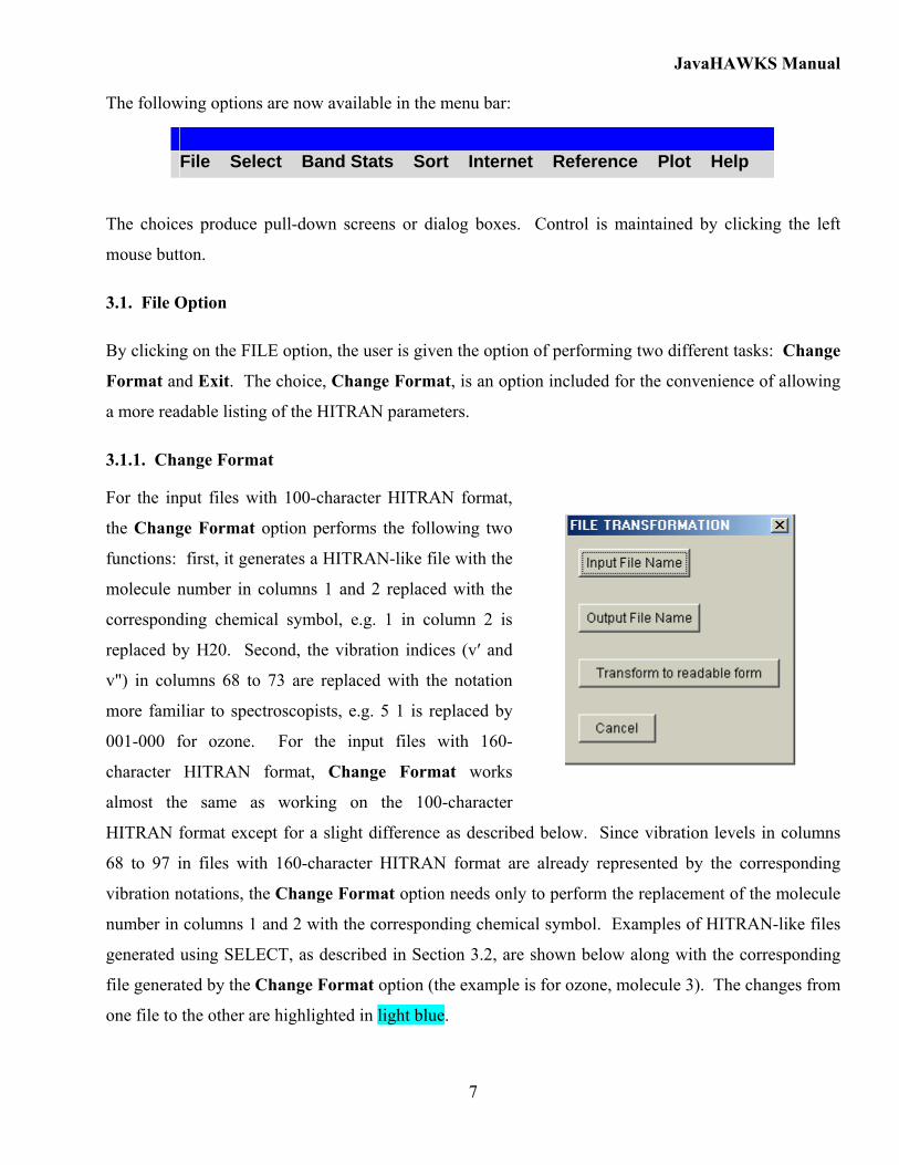
The option is simply run. “Input File Name” is the name of the HITRAN-like file you wish to
transform into the new format. “Output File Name” is the name you select for the new file. The action
is initiated by selecting “Transform to readable form”, and the action is canceled by selection of the
“Cancel” option.
3.1.2. Exit
The Exit option enables an easy exit from the JavaHAWKS software.
3.2. Select Option
The most important and detailed option screen is Select, which
contains several choices described below.
Select is the principal operating program for a detailed
manipulation of the HITRAN database, or any files in the
HITRAN format. When SELECT is started, a set of default
parameters, from your previous run, is retained.
JavaHAWKS Manual
9
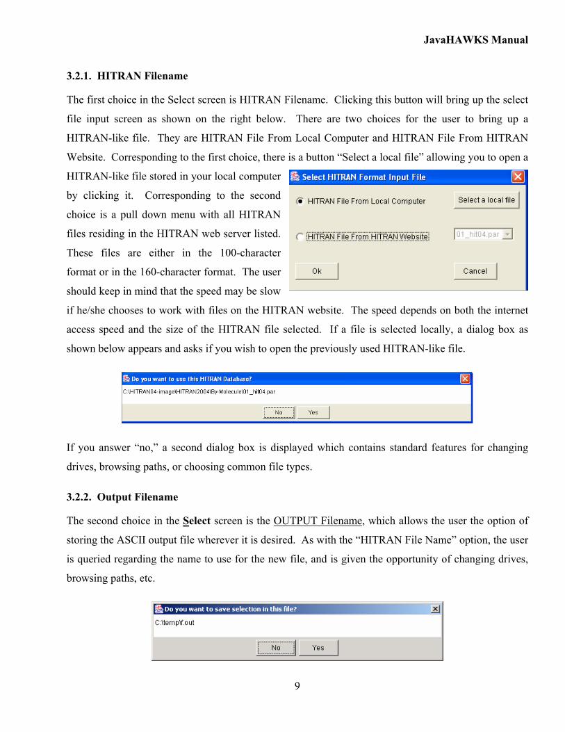
3.2.1. HITRAN Filename
The first choice in the Select screen is HITRAN Filename. Clicking this button will bring up the select
file input screen as shown on the right below. There are two choices for the user to bring up a
HITRAN-like file. They are HITRAN File From Local Computer and HITRAN File From HITRAN
Website. Corresponding to the first choice, there is a button “Select a local file” allowing you to open a
HITRAN-like file stored in your local computer
by clicking it. Corresponding to the second
choice is a pull down menu with all HITRAN
files residing in the HITRAN web server listed.
These files are either in the 100-character
format or in the 160-character format. The user
should keep in mind that the speed may be slow
if he/she chooses to work with files on the HITRAN website. The speed depends on both the internet
access speed and the size of the HITRAN file selected. If a file is selected locally, a dialog box as
shown below appears and asks if you wish to open the previously used HITRAN-like file.
If you answer “no,” a second dialog box is displayed which contains standard features for changing
drives, browsing paths, or choosing common file types.
3.2.2. Output Filename
The second choice in the Select screen is the OUTPUT Filename, which allows the user the option of
storing the ASCII output file wherever it is desired. As with the “HITRAN File Name” option, the user
is queried regarding the name to use for the new file, and is given the opportunity of changing drives,
browsing paths, etc.

JavaHAWKS Manual
10
If you answer “No”, it will ask you again to locate the place to store the new file. If you answer “yes”
and the file the user selects already exists, the dialog below will ask you if you really want to overwrite
the existing file.
The Select function allows the user to generate a file in either the standard HITRAN format, or as a
comma-separated values file (or both). The format of the latter file is based on the column definitions
of the HITRAN database, and is of use to users who want to open the file with a program that delimits
the file based on comma separators, e.g. Microsoft Excel®. An example of a comma-separated file,
corresponding to the examples shown in Section 3.1.1 above, is given below:
3,2,1000.003800, 1.620E-23, 1.498E-02,.0706,.0908, 497.2245, .76, .000000, 5, 1,26 819 ,27 820 ,005, 1 1 1 3,2,1000.003800, 1.620E-23, 1.498E-02,.0706,.0908, 497.2245, .76, .000000, 5, 1,26 818 ,27 819 ,005, 1 1 1 3,1,1000.010100, 1.340E-24, 1.461E-02,.0709,.0912, 2246.4110, .76, .000000, 18, 7,22 914 ,21 913 ,005, 1 1 1 3,1,1000.010700, 4.800E-24, 4.964E-02,.0748,.1026, 2168.1560, .76, .000000, 27, 14,16 215 ,15 214 ,455, 4 4 1 3,1,1000.012900, 6.440E-24, 2.258E-03,.0707,.0919, 1597.2180, .76, .000000, 13, 4,28 722 ,28 721 ,005, 1 1 1
3.2.3. Spectral Range
The third choice in this series is Spectral Range, which
allows the user to identify the wavenumber (or wavelength)
range of the data being gathered. One can choose the start
and end of the selection in either wavenumber (cm-1) or
wavelength (µm). This option is the essential choice
(necessary and sufficient) in any SELECT procedure.
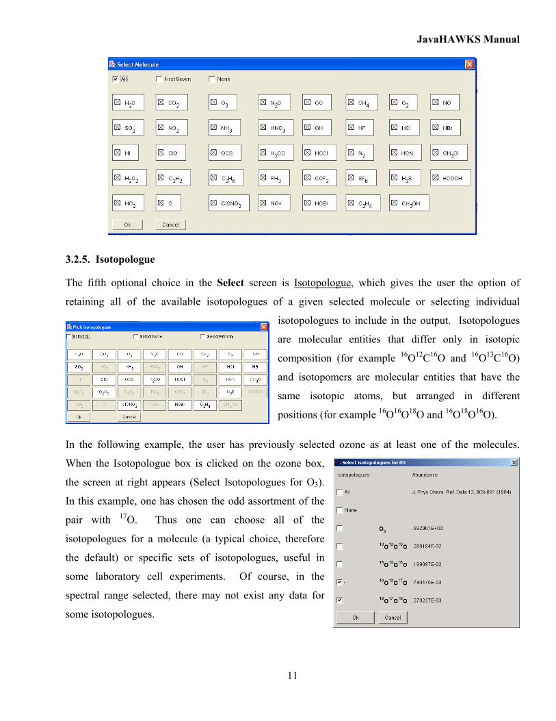
3.2.4. Molecule
The fourth optional choice in the Select screen is Molecule, which gives the user the option of
including All the available molecules within the spectral range defined, the First 7 molecules
(coinciding to the original HITRAN), or None. None is provided as a convenient button to allow the
user to subsequently select various specific assortments of molecules; hence this choice is probably the
most frequently employed.
JavaHAWKS Manual
11
3.2.5. Isotopologue
The fifth optional choice in the Select screen is Isotopologue, which gives the user the option of
retaining all of the available isotopologues of a given selected molecule or selecting individual
isotopologues to include in the output. Isotopologues
are molecular entities that differ only in isotopic
composition (for example 16O12C16O and 16O13C16O)
and isotopomers are molecular entities that have the
same isotopic atoms, but arranged in different
positions (for example 16O16O18O and 16O18O16O).
In the following example, the user has previously selected ozone as at least one of the molecules.
When the Isotopologue box is clicked on the ozone box,
the screen at right appears (Select Isotopologues for O3).
In this example, one has chosen the odd assortment of the
pair with 17O. Thus one can choose all of the
isotopologues for a molecule (a typical choice, therefore
the default) or specific sets of isotopologues, useful in
some laboratory cell experiments. Of course, in the
spectral range selected, there may not exist any data for
some isotopologues.
JavaHAWKS Manual
12
The actual values of isotopic abundances used in HITRAN are given in the second column in the
isotopologue selection box. These values enable the user to re-normalize the intensities, for example
where the output is to correspond to a laboratory absorption experiment with enhanced isotopic
mixtures.
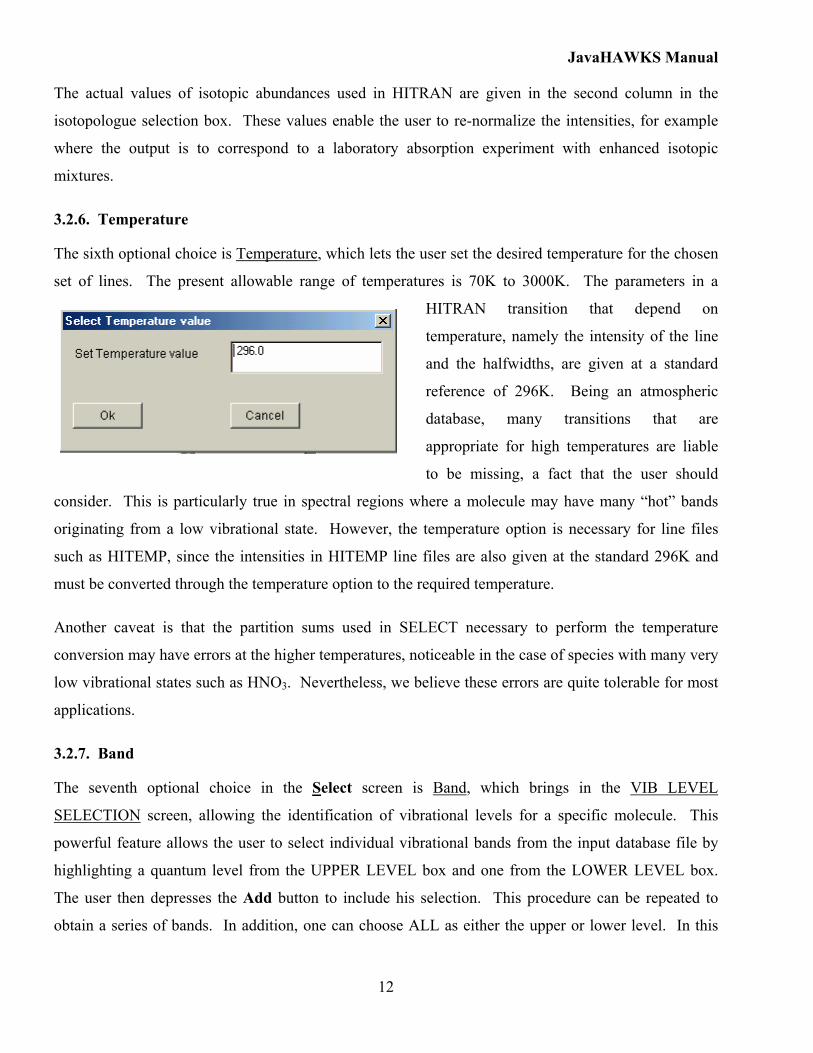
3.2.6. Temperature
The sixth optional choice is Temperature, which lets the user set the desired temperature for the chosen
set of lines. The present allowable range of temperatures is 70K to 3000K. The parameters in a
HITRAN transition that depend on
temperature, namely the intensity of the line
and the halfwidths, are given at a standard
reference of 296K. Being an atmospheric
database, many transitions that are
appropriate for high temperatures are liable
to be missing, a fact that the user should
consider. This is particularly true in spectral regions where a molecule may have many “hot” bands
originating from a low vibrational state. However, the temperature option is necessary for line files
such as HITEMP, since the intensities in HITEMP line files are also given at the standard 296K and
must be converted through the temperature option to the required temperature.
Another caveat is that the partition sums used in SELECT necessary to perform the temperature
conversion may have errors at the higher temperatures, noticeable in the case of species with many very
low vibrational states such as HNO3. Nevertheless, we believe these errors are quite tolerable for most
applications.
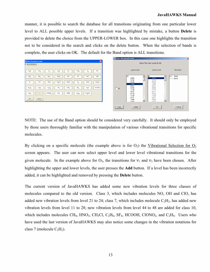
3.2.7. Band
The seventh optional choice in the Select screen is Band, which brings in the VIB LEVEL
SELECTION screen, allowing the identification of vibrational levels for a specific molecule. This
powerful feature allows the user to select individual vibrational bands from the input database file by
highlighting a quantum level from the UPPER LEVEL box and one from the LOWER LEVEL box.
The user then depresses the Add button to include his selection. This procedure can be repeated to
obtain a series of bands. In addition, one can choose ALL as either the upper or lower level. In this
JavaHAWKS Manual
13
manner, it is possible to search the database for all transitions originating from one particular lower
level to ALL possible upper levels. If a transition was highlighted by mistake, a button Delete is
provided to delete the choice from the UPPER-LOWER box. In this case one highlights the transition
not to be considered in the search and clicks on the delete button. When the selection of bands is
complete, the user clicks on OK. The default for the Band option is ALL transitions.
NOTE: The use of the Band option should be considered very carefully. It should only be employed
by those users thoroughly familiar with the manipulation of various vibrational transitions for specific
molecules.
By clicking on a specific molecule (the example above is for O3) the Vibrational Selection for O3
screen appears. The user can now select upper level and lower level vibrational transitions for the
given molecule. In the example above for O3, the transitions for ν1 and ν3 have been chosen. After
highlighting the upper and lower levels, the user presses the Add button. If a level has been incorrectly
added, it can be highlighted and removed by pressing the Delete button.
The current version of JavaHAWKS has added some new vibration levels for three classes of
molecules compared to the old version. Class 3, which includes molecules NO, OH and ClO, has
added new vibration levels from level 21 to 24; class 7, which includes molecule C2H2, has added new
vibration levels from level 11 to 28; new vibration levels from level 44 to 48 are added for class 10,
which includes molecules CH4, HNO3, CH3Cl, C2H6, SF6, HCOOH, ClONO2, and C2H4. Users who
have used the last version of JavaHAWKS may also notice some changes in the vibration notations for
class 7 (molecule C2H2).

JavaHAWKS Manual
14
3.2.8. Cutoff
The eighth optional choice in the Select screen is Cutoff, which gives the user the option of eliminating
lines below a specified intensity. To implement, one types in the threshold intensity in exponent
notation. JavaHAWKS will convert the exponent to a 3-digit value even if one number is typed in, e.g.
2.3E-9 becomes 2.3e-009. There are some transitions in HITRAN, and many in HITEMP, whose
intensities (given at the standard 296K) are less than the single precision allowed by most compilers. In
that case Cutoff can be used to eliminate them from the
selected output.
NOTE: This Cutoff option can be used to limit the dynamic
range, but one generally does not know, a priori, what the
overall effect on simulations that use the output file will be. Therefore, this option, as with the choice
of Band, is probably only useful to very experienced users of the database. Since the plotting package
(see Section 3.6) allows control of the minimum plotted intensity, this cutoff option does not need to be
used for that purpose.
3.2.9. RUN SELECT
The ninth choice in the Select option is RUN SELECT, which when activated, will produce an outline
of the chosen case to run, as shown in the following example. This box is provided as a rough check
for the user to verify his/her choices. If the output file already exists, a warning message will appear on
this box.

JavaHAWKS Manual
15
By clicking on the OK button the Select program will begin its operation. As the program is searching
the database to select the desired lines, a window is displayed with a “thermometer” which indicates the
progress of the selection process.
3.2.10. RUN DESELECT
The RUN DESELECT option is provided to the user to perform the inverse operation on the HITRAN
database to Select. The concept here is to allow an editing feature for subtracting old or unwanted
bands from a database and leaving the skeleton database to which one subsequently may add new or
replacement data. One proceeds with the same selection criteria as one would in a normal Select
procedure. The current version of this software extends the deselecting function to both isotopologues
and bands, which was not the case in earlier versions of the software. In addition, in older versions of
this software the choice of spectral interval was ignored: the initial database being “deselected” is taken
in full. However, that IS NOT THE CASE with the current version. Only lines between the initial
and final wavenumber (wavelength) will be given in the resulting output file. One should note that
ample disk space needs to be considered in the general case of deselecting a few bands of a molecule
from the HITRAN database. The resulting database that is written may very well be almost the same
size as the original.
3.3. Band Stats Option
The Band Stats option runs the Bandsum program on a given file of data, or on the entire HITRAN
database, for one or more molecules. The output gives: the number of lines for every band of each
isotopologue; the minimum and maximum wavenumber, J values, line intensities, broadening
parameters, line shift; sum of the line intensities; and
additional spectroscopic statistics of use for in-depth
analysis. At the end of the output, a new section called
Summary of Missing Bands is attached. Information
contained in each line of this section includes the missing
upper and lower vibrations for a specific molecule and
isotopologue. This is a new feature to the previous version
of JavaHAWKS. The program accessed by selecting the
Band Stats option from the main menu will give the
dialog box as shown here.
JavaHAWKS Manual
16
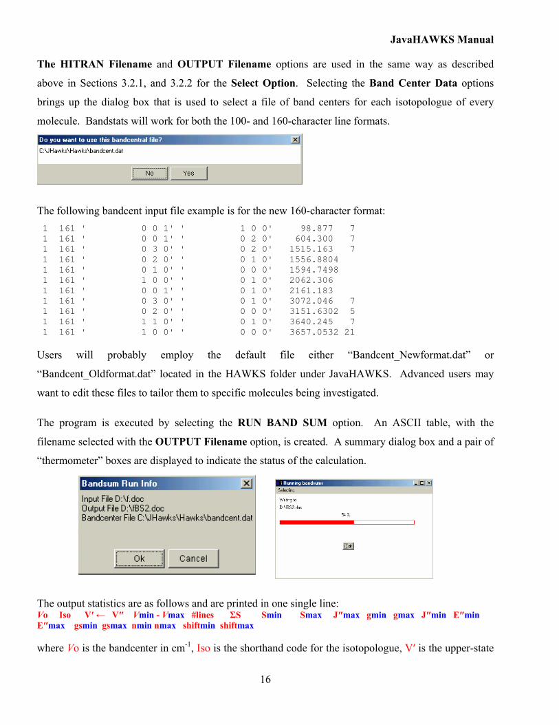
The HITRAN Filename and OUTPUT Filename options are used in the same way as described
above in Sections 3.2.1, and 3.2.2 for the Select Option. Selecting the Band Center Data options
brings up the dialog box that is used to select a file of band centers for each isotopologue of every
molecule. Bandstats will work for both the 100- and 160-character line formats.
The following bandcent input file example is for the new 160-character format: 1 161 ' 0 0 1' ' 1 0 0' 98.877 7 1 161 ' 0 0 1' ' 0 2 0' 604.300 7 1 161 ' 0 3 0' ' 0 2 0' 1515.163 7 1 161 ' 0 2 0' ' 0 1 0' 1556.8804 1 161 ' 0 1 0' ' 0 0 0' 1594.7498 1 161 ' 1 0 0' ' 0 1 0' 2062.306 1 161 ' 0 0 1' ' 0 1 0' 2161.183 1 161 ' 0 3 0' ' 0 1 0' 3072.046 7 1 161 ' 0 2 0' ' 0 0 0' 3151.6302 5 1 161 ' 1 1 0' ' 0 1 0' 3640.245 7 1 161 ' 1 0 0' ' 0 0 0' 3657.0532 21
Users will probably employ the default file either “Bandcent_Newformat.dat” or
“Bandcent_Oldformat.dat” located in the HAWKS folder under JavaHAWKS. Advanced users may
want to edit these files to tailor them to specific molecules being investigated.
The program is executed by selecting the RUN BAND SUM option. An ASCII table, with the
filename selected with the OUTPUT Filename option, is created. A summary dialog box and a pair of
“thermometer” boxes are displayed to indicate the status of the calculation.
The output statistics are as follows and are printed in one single line: Vo Iso V′ ← V″ Vmin - Vmax #lines ΣS Smin Smax J″max gmin gmax J″min E″min E″max gsmin gsmax nmin nmax shiftmin shiftmax
where Vo is the bandcenter in cm-1, Iso is the shorthand code for the isotopologue, V′ is the upper-state
JavaHAWKS Manual
17
vibrational band quanta, V″ is the lower-state vibrational band quanta, Vmin is the minimum
wavenumber found for the band (rounded down to the nearest integer wavenumber), Vmax is the
maximum wavenumber found for the band (rounded up to the nearest integer wavenumber), #lines is
the number of transitions found for the band, ΣS is the sum of intensities in the band, Smin is the
minimum intensity in the band, Smax is the maximum intensity in the band, J″max is the maximum lower-
state rotational quantum value found. On the second line for the band, gmin is the minimum value of
air-broadened halfwidth, gmax is the maximum value of air-broadened halfwidth, J″min is the minimum
lower-state rotational quantum value found, E″min is the minimum lower-state energy, E″max is the
maximum lower-state energy, gsmin is the minimum value of self-broadened halfwidth, gsmax is the
maximum value of self-broadened halfwidth, nmin is the minimum value of the temperature-dependence
coefficient, nmax is the maximum value of the temperature-dependence coefficient, shiftmin is the
maximum value of self-broadened halfwidth, is the minimum value of the pressure-shift, and shiftmax is
the maximum value of the pressure-shift.
If you request a band in the bandcent.dat input file that is not found in the HITRAN-like file, the output
will indicate zero lines, and pre-set extrema will be given for the ranges (50000 for the minima, and 0
for the maxima). On the other hand, if a band exists in the HITRAN file that was not requested in the
bandcent.dat file, a summary is indicated at end of the output to inform you that you may want to add
this band to your search.
3.4. Sort Option
The Sort option allows the user to sort by wavenumber of a HITRAN-like file (the field defined by
positions 4 through 15), or to merge numerous individual HITRAN-like files into a single file.
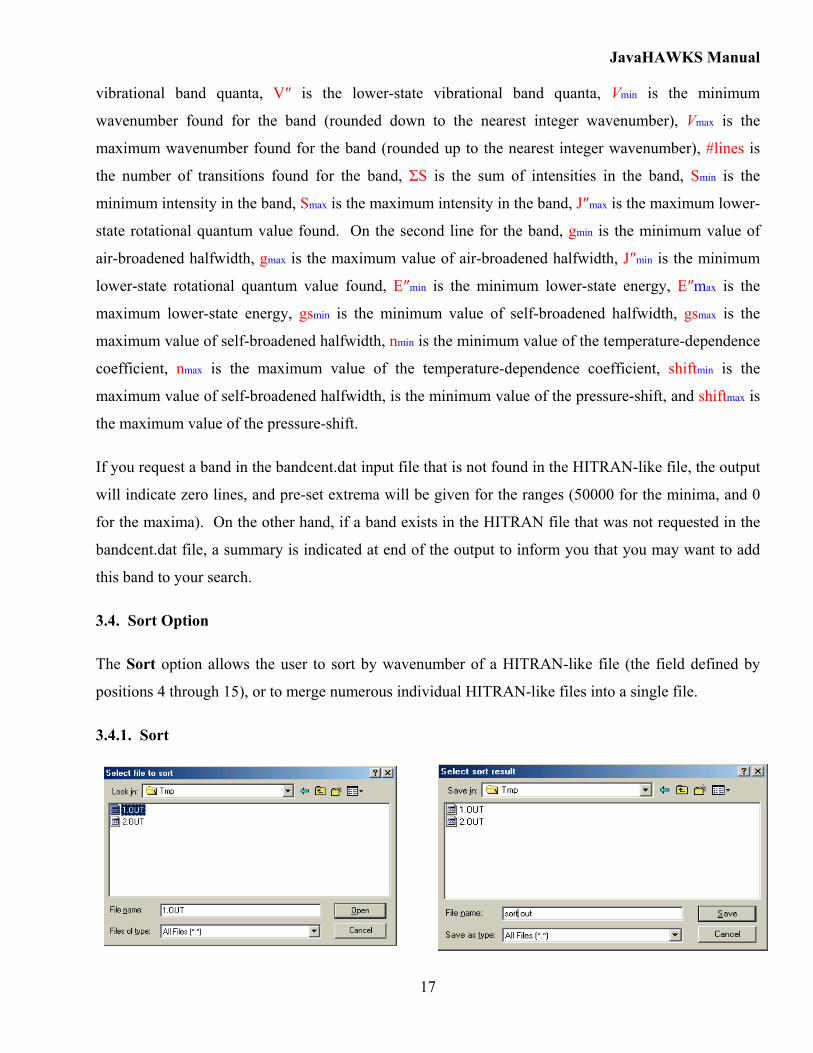
3.4.1. Sort
JavaHAWKS Manual
18
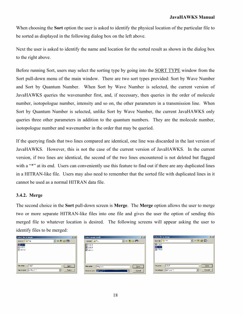
When choosing the Sort option the user is asked to identify the physical location of the particular file to
be sorted as displayed in the following dialog box on the left above.
Next the user is asked to identify the name and location for the sorted result as shown in the dialog box
to the right above.
Before running Sort, users may select the sorting type by going into the SORT TYPE window from the
Sort pull-down menu of the main window. There are two sort types provided: Sort by Wave Number
and Sort by Quantum Number. When Sort by Wave Number is selected, the current version of
JavaHAWKS queries the wavenumber first, and, if necessary, then queries in the order of molecule
number, isotopologue number, intensity and so on, the other parameters in a transmission line. When
Sort by Quantum Number is selected, unlike Sort by Wave Number, the current JavaHAWKS only
queries three other parameters in addition to the quantum numbers. They are the molecule number,
isotopologue number and wavenumber in the order that may be queried.
If the querying finds that two lines compared are identical, one line was discarded in the last version of
JavaHAWKS. However, this is not the case of the current version of JavaHAWKS. In the current
version, if two lines are identical, the second of the two lines encountered is not deleted but flagged
with a “*” at its end. Users can conveniently use this feature to find out if there are any duplicated lines
in a HITRAN-like file. Users may also need to remember that the sorted file with duplicated lines in it
cannot be used as a normal HITRAN data file.
3.4.2. Merge
The second choice in the Sort pull-down screen is Merge. The Merge option allows the user to merge
two or more separate HITRAN-like files into one file and gives the user the option of sending this
merged file to whatever location is desired. The following screens will appear asking the user to
identify files to be merged:
JavaHAWKS Manual
19
Click on the CANCEL button to end the selection of files being merged. A new dialog box will now
appear (at the right above) directing the naming of the file containing the merged results.
NOTE: Merge will also sort the resulting file, if (and only if), the lines in the individual HITRAN files
are already in order of increasing wavenumber. If there is an identical line existing in more than one
file to be merged (that is there is an overlap between files), this line will be duplicated but flagged at its
end with a “*” except the first one in the merging resulting file. Users may need to remember that the
merged file with duplicated lines in it can not be used as a normal HITRAN data file.
3.5. Internet Option
The Internet option has been added to the main menu bar in the latest version of JavaHAWKS. This
option allows users to interact with the outside world through the Internet by providing access to the
HITRAN database and other data sources. There are five choices under the Internet option. They are
HITRAN Website, HITRAN FTP Site, JPL Submillimeter Data, Cologne Spectroscopy Data, and CfA
UV Xsection Data.
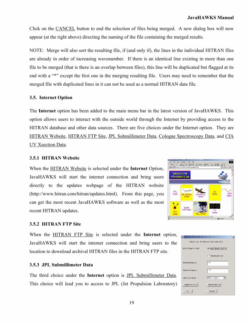
3.5.1 HITRAN Website
When the HITRAN Website is selected under the Internet Option,
JavaHAWKS will start the internet connection and bring users
directly to the updates webpage of the HITRAN website
(http://www.hitran.com/hitran/updates.html). From this page, you
can get the most recent JavaHAWKS software as well as the most
recent HITRAN updates.
3.5.2 HITRAN FTP Site
When the HITRAN FTP Site is selected under the Internet option,
JavaHAWKS will start the internet connection and bring users to the
location to download archival HITRAN files in the HITRAN FTP site.
3.5.3 JPL Submillimeter Data
The third choice under the Internet option is JPL Submillimeter Data.
This choice will lead you to access to JPL (Jet Propulsion Laboratory)
JavaHAWKS Manual
20
submillimeter catalog,7 download a JPL catalog file from the database and then convert the downloaded
data into a HITRAN format file. Selection of this item will bring in a screen called Downloading Data
From JPL and Converting Into HITRAN File, which lets you set up the downloading parameters. The
parameters include wavenumber units (in wavenumber or in wavelength), minimum wavenumber,
maximum wavenumber and the molecule you are interested in. The Output File Name button will ask
you to specify a location to save the converted data. Pressing the Browse Internet button will initialize
the data downloading over the internet and then the conversion to a HITRAN format file. This
reformatting includes converting the line intensities to the HITRAN units and standard of 296K,
changing the vibrational notation, and converting the JPL error bars to the HITRAN system. Since the
JPL catalog does not contain information about collision-broadening, these parameters are left blank in
the conversion to the HITRAN-like file. A file with the data in its original format will also be saved
under the current JavaHAWKS working directory.
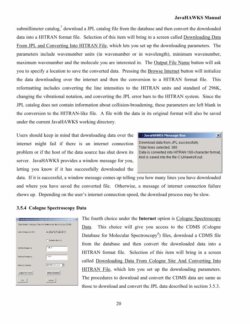
Users should keep in mind that downloading data over the
internet might fail if there is an internet connection
problem or if the host of the data source has shut down its
server. JavaHAWKS provides a window message for you,
letting you know if it has successfully downloaded the
data. If it is successful, a window message comes up telling you how many lines you have downloaded
and where you have saved the converted file. Otherwise, a message of internet connection failure
shows up. Depending on the user’s internet connection speed, the download process may be slow.
3.5.4 Cologne Spectroscopy Data
The fourth choice under the Internet option is Cologne Spectroscopy
Data. This choice will give you access to the CDMS (Cologne
Database for Molecular Spectroscopy8) files, download a CDMS file
from the database and then convert the downloaded data into a
HITRAN format file. Selection of this item will bring in a screen
called Downloading Data From Cologne Site And Converting Into
HITRAN File, which lets you set up the downloading parameters.
The procedures to download and convert the CDMS data are same as
those to download and convert the JPL data described in section 3.5.3.

JavaHAWKS Manual
21
3.5.5 CfA UV Xsection Data
The fifth choice under the Internet option is CfA UV
Xsection Data. This choice allows you to download UV
cross-section data from the molecular database at the
Harvard-Smithsonian Center for Astrophysics (CfA) and to
convert the data to a file with the HITRAN cross-section file
format. Selecting this choice will bring up a screen listing
those molecules with available UV cross-section data files.
More than one UV cross-section data file exists for each molecule in the molecular database at the CfA.
Clicking on the molecule that you are interested in will bring up the next screen, which allows you to
select one of the UV cross section data files. Specify the location you want to save the converted cross
section file in HITRAN format. Clicking the Browse And Convert button will complete the process of
data downloading and converting. The CfA absorption cross-section data are listed linearly in
wavelength; the conversion to HITRAN format has created a grid linear in wavenumber. Again,
downloading data over the internet may fail if there is an internet connection problem or if the host of
the data source has shut down its server. A message box will come up, indicating success or failure of
the downlaod.
3.6. Reference Option
The next pull-down screen is Reference. It contains three separate options: Molecule, Wavenumber,
and Xsection, for obtaining information on references utilized in creating the database. If you are using
JavaHAWKS for the first time, these three options will be “grayed” out. The reference files are in the
Adobe portable document format (pdf). Java is unable to search for the appropriate reader; you must
point the JavaHAWKS software to the correct location of either the Adobe reader or Adobe Acrobat.
You do this by selecting the “Acrobat Reader” in the dialog box shown below. You may wish to

JavaHAWKS Manual
22
consult your system administrator if you cannot find the
reader, or are uncertain of how to proceed. Copies of the
reader can be obtained from Adobe by using the link
contained in the HITRAN web-site under the
documentation sub-page.
After the reader has been selected, the “Molecule”,
“Wavelength”, and “Xsection” options will be active.
3.6.1. Molecule
The first option, Molecule, allows the user to address the molecular reference table utilized by the
HITRAN database for identifying the series of references for the line position, line intensity, and air-
broadened halfwidth. Selection of this option will open the Adobe reader with the corresponding
molecule pdf file. From links in this reference table, you can obtain the abstracts relating to the
HITRAN parameters (such as line positions, line intensity and air-broadened halfwidth) of a line stored
in HITRAN database.
3.6.2. Wavenumber
This feature is yet to be implemented in the JavaHAWKS software. It will be added in a future
version.
3.6.3. Xsection
The third option in the Reference pull down screen is Xsection. Selection of this option will open the
Adobe reader with the corresponding cross-section references.
3.7. Plot Option
The sixth optional screen is Plot. The JavaHAWKS Plot screen has two selections: “Plot Line by
Line”, which allows the user to plot the “Intensity”, “Transition Probability Squared” in the 100-
character format (“Einstein-A coefficient” in the 160-character format), or “Lower State Energy” from
HITRAN-like files as a function of wavenumber; and “Plot Xsection”, which allows the user to plot the
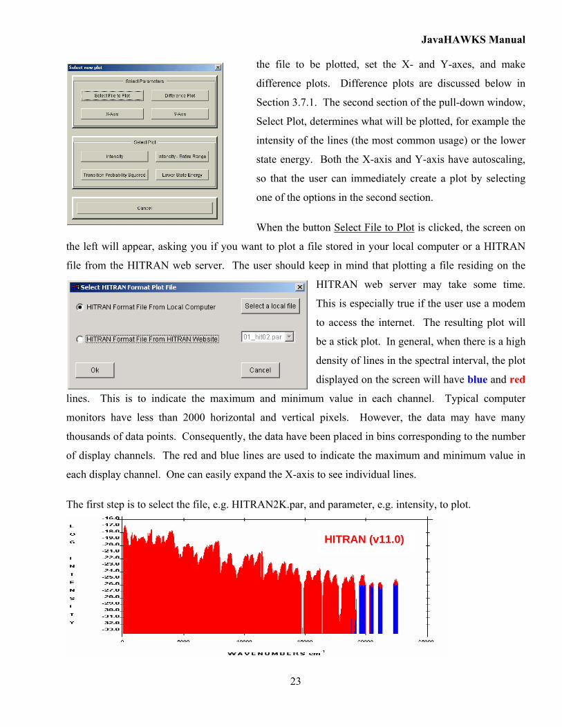
cross-section data as a function of wavenumber. Selecting “Plot Line by Line” will display the screen
shown here. This screen is divided into sections. The upper section, Select Parameters, is used to open
JavaHAWKS Manual
23
the file to be plotted, set the X- and Y-axes, and make
difference plots. Difference plots are discussed below in
Section 3.7.1. The second section of the pull-down window,
Select Plot, determines what will be plotted, for example the
intensity of the lines (the most common usage) or the lower
state energy. Both the X-axis and Y-axis have autoscaling,
so that the user can immediately create a plot by selecting
one of the options in the second section.
When the button Select File to Plot is clicked, the screen on
the left will appear, asking you if you want to plot a file stored in your local computer or a HITRAN
file from the HITRAN web server. The user should keep in mind that plotting a file residing on the
HITRAN web server may take some time.
This is especially true if the user use a modem
to access the internet. The resulting plot will
be a stick plot. In general, when there is a high
density of lines in the spectral interval, the plot
displayed on the screen will have blue and red
lines. This is to indicate the maximum and minimum value in each channel. Typical computer
monitors have less than 2000 horizontal and vertical pixels. However, the data may have many
thousands of data points. Consequently, the data have been placed in bins corresponding to the number
of display channels. The red and blue lines are used to indicate the maximum and minimum value in
each display channel. One can easily expand the X-axis to see individual lines.
The first step is to select the file, e.g. HITRAN2K.par, and parameter, e.g. intensity, to plot.
HITRAN (v11.0)
JavaHAWKS Manual
24
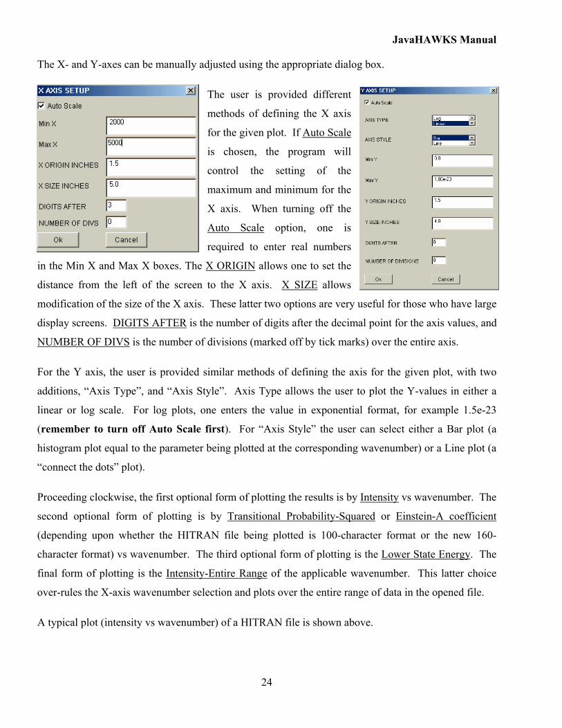
The X- and Y-axes can be manually adjusted using the appropriate dialog box.
The user is provided different
methods of defining the X axis
for the given plot. If Auto Scale
is chosen, the program will
control the setting of the
maximum and minimum for the
X axis. When turning off the
Auto Scale option, one is
required to enter real numbers
in the Min X and Max X boxes. The X ORIGIN allows one to set the
distance from the left of the screen to the X axis. X SIZE allows
modification of the size of the X axis. These latter two options are very useful for those who have large
display screens. DIGITS AFTER is the number of digits after the decimal point for the axis values, and
NUMBER OF DIVS is the number of divisions (marked off by tick marks) over the entire axis.
For the Y axis, the user is provided similar methods of defining the axis for the given plot, with two
additions, “Axis Type”, and “Axis Style”. Axis Type allows the user to plot the Y-values in either a
linear or log scale. For log plots, one enters the value in exponential format, for example 1.5e-23
(remember to turn off Auto Scale first). For “Axis Style” the user can select either a Bar plot (a
histogram plot equal to the parameter being plotted at the corresponding wavenumber) or a Line plot (a
“connect the dots” plot).
Proceeding clockwise, the first optional form of plotting the results is by Intensity vs wavenumber. The
second optional form of plotting is by Transitional Probability-Squared or Einstein-A coefficient
(depending upon whether the HITRAN file being plotted is 100-character format or the new 160-
character format) vs wavenumber. The third optional form of plotting is the Lower State Energy. The
final form of plotting is the Intensity-Entire Range of the applicable wavenumber. This latter choice
over-rules the X-axis wavenumber selection and plots over the entire range of data in the opened file.
A typical plot (intensity vs wavenumber) of a HITRAN file is shown above.

JavaHAWKS Manual
25
3.7.1 Difference Plot
This option lets the user take the difference of two spectral plots. This can be a useful tool to
determine small shifts in wavenumber (or line strength) between two files. The following screen is
displayed when the Difference Plot option is selected:
After selecting the first file, the user is prompted to select the second file (the second file is subtracted
from the first). We will use f1.out and f2.out as an example to show how Dif file works. A stick plot
of f1.out is shown below:
The second file (f2.out) is identical to the first except that the line at 19100.3239 cm-1 has been shifted
to 19100.43239cm-1. After the two files have been selected, the user is prompted to input a normalized
scaling width, which is a value between 0 and 1
(see the figure on left). We have arbitrarily chosen
a Doppler line shape to broaden the lines for
subtraction. This is not an attempt to simulate a
spectroscopic feature, but simply a means chosen to
JavaHAWKS Manual
26
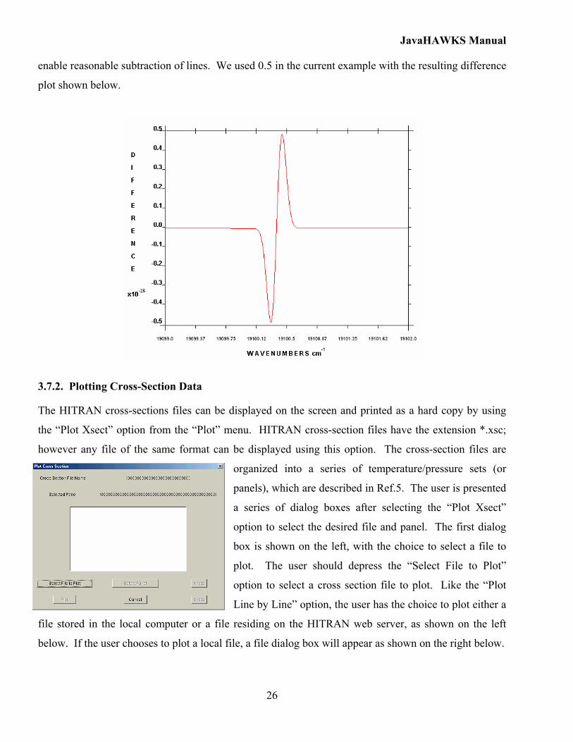
enable reasonable subtraction of lines. We used 0.5 in the current example with the resulting difference
plot shown below.
3.7.2. Plotting Cross-Section Data
The HITRAN cross-sections files can be displayed on the screen and printed as a hard copy by using
the “Plot Xsect” option from the “Plot” menu. HITRAN cross-section files have the extension *.xsc;
however any file of the same format can be displayed using this option. The cross-section files are
organized into a series of temperature/pressure sets (or
panels), which are described in Ref.5. The user is presented
a series of dialog boxes after selecting the “Plot Xsect”
option to select the desired file and panel. The first dialog
box is shown on the left, with the choice to select a file to
plot. The user should depress the “Select File to Plot”
option to select a cross section file to plot. Like the “Plot
Line by Line” option, the user has the choice to plot either a
file stored in the local computer or a file residing on the HITRAN web server, as shown on the left
below. If the user chooses to plot a local file, a file dialog box will appear as shown on the right below.
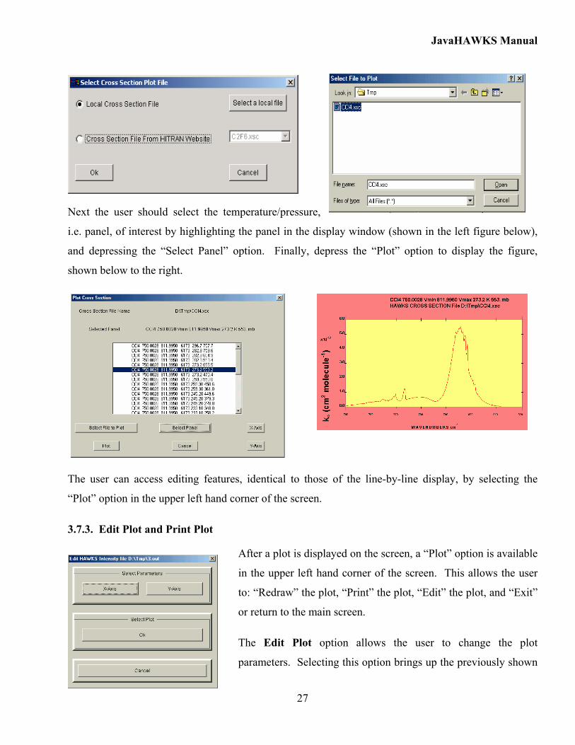
JavaHAWKS Manual
27
Next the user should select the temperature/pressure,
i.e. panel, of interest by highlighting the panel in the display window (shown in the left figure below),
and depressing the “Select Panel” option. Finally, depress the “Plot” option to display the figure,
shown below to the right.
The user can access editing features, identical to those of the line-by-line display, by selecting the
“Plot” option in the upper left hand corner of the screen.
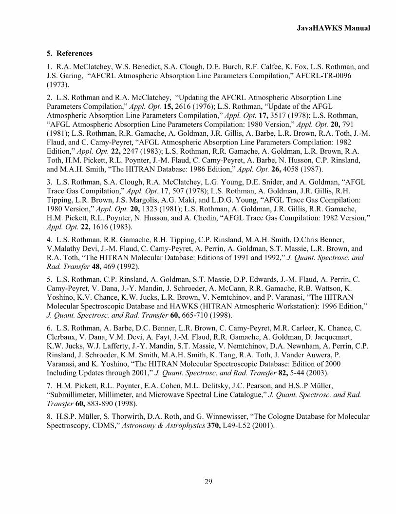
3.7.3. Edit Plot and Print Plot
After a plot is displayed on the screen, a “Plot” option is available
in the upper left hand corner of the screen. This allows the user
to: “Redraw” the plot, “Print” the plot, “Edit” the plot, and “Exit”
or return to the main screen.
The Edit Plot option allows the user to change the plot
parameters. Selecting this option brings up the previously shown

JavaHAWKS Manual
28
X axis and Y axis dialog boxes. The X axis and Y axis choices have the same functions as described
above.
A hard copy of the plot displayed on the screen can be made by using the “Print” options.
3.8. Help Option
The eighth optional pull down screen is Help. This option gives the user informative help on all of the
molecules stored in the database as well as pertinent information on the structure and uses of the
HITRAN database. A complete informative package of information on all of the molecules and
isotopologues is provided within the Help pull-down menu. You can find historical documentation
about the HITRAN database, from earliest HITRAN documentation (1973) to the most recent
documentation. This informative package consists of pdf files and users can open them with Acrobat
Reader to find relevant information.
3.8.1. About
Another choice in the HELP section is About, which is a standard statement describing the
construction of the JavaHAWKS program for the HITRAN database.
4. Acknowledgments
The contributors to the spectroscopy of this effort are too numerous to cite here. We urge users of
JavaHAWKS to consult the references contained on all transitions updated since 1986, and we
apologize for any omissions or oversights that may have been made.
The current effort for the HITRAN compilation has been supported by the NASA Earth Observing
System (EOS), grant NAG5-8420; the NASA Upper Atmospheric Research Satellite (UARS) program;
the Atmospheric Radiation Measurement (ARM) program of the Biological and Environmental
Research Program (BER), US Department of Energy, Grant No. DE-FG02-00ER62930; the Air Force
Research Laboratory, Hanscom AFB; and internal funding from the Smithsonian Institution.
JavaHAWKS Manual
29
5. References
1. R.A. McClatchey, W.S. Benedict, S.A. Clough, D.E. Burch, R.F. Calfee, K. Fox, L.S. Rothman, and J.S. Garing, “AFCRL Atmospheric Absorption Line Parameters Compilation,” AFCRL-TR-0096 (1973).
2. L.S. Rothman and R.A. McClatchey, “Updating the AFCRL Atmospheric Absorption Line Parameters Compilation,” Appl. Opt. 15, 2616 (1976); L.S. Rothman, “Update of the AFGL Atmospheric Absorption Line Parameters Compilation,” Appl. Opt. 17, 3517 (1978); L.S. Rothman, “AFGL Atmospheric Absorption Line Parameters Compilation: 1980 Version,” Appl. Opt. 20, 791 (1981); L.S. Rothman, R.R. Gamache, A. Goldman, J.R. Gillis, A. Barbe, L.R. Brown, R.A. Toth, J.-M. Flaud, and C. Camy-Peyret, “AFGL Atmospheric Absorption Line Parameters Compilation: 1982 Edition,” Appl. Opt. 22, 2247 (1983); L.S. Rothman, R.R. Gamache, A. Goldman, L.R. Brown, R.A. Toth, H.M. Pickett, R.L. Poynter, J.-M. Flaud, C. Camy-Peyret, A. Barbe, N. Husson, C.P. Rinsland, and M.A.H. Smith, “The HITRAN Database: 1986 Edition,” Appl. Opt. 26, 4058 (1987).
3. L.S. Rothman, S.A. Clough, R.A. McClatchey, L.G. Young, D.E. Snider, and A. Goldman, “AFGL Trace Gas Compilation,” Appl. Opt. 17, 507 (1978); L.S. Rothman, A. Goldman, J.R. Gillis, R.H. Tipping, L.R. Brown, J.S. Margolis, A.G. Maki, and L.D.G. Young, “AFGL Trace Gas Compilation: 1980 Version,” Appl. Opt. 20, 1323 (1981); L.S. Rothman, A. Goldman, J.R. Gillis, R.R. Gamache, H.M. Pickett, R.L. Poynter, N. Husson, and A. Chedin, “AFGL Trace Gas Compilation: 1982 Version,” Appl. Opt. 22, 1616 (1983).
4. L.S. Rothman, R.R. Gamache, R.H. Tipping, C.P. Rinsland, M.A.H. Smith, D.Chris Benner, V.Malathy Devi, J.-M. Flaud, C. Camy-Peyret, A. Perrin, A. Goldman, S.T. Massie, L.R. Brown, and R.A. Toth, “The HITRAN Molecular Database: Editions of 1991 and 1992,” J. Quant. Spectrosc. and Rad. Transfer 48, 469 (1992).
5. L.S. Rothman, C.P. Rinsland, A. Goldman, S.T. Massie, D.P. Edwards, J.-M. Flaud, A. Perrin, C. Camy-Peyret, V. Dana, J.-Y. Mandin, J. Schroeder, A. McCann, R.R. Gamache, R.B. Wattson, K. Yoshino, K.V. Chance, K.W. Jucks, L.R. Brown, V. Nemtchinov, and P. Varanasi, “The HITRAN Molecular Spectroscopic Database and HAWKS (HITRAN Atmospheric Workstation): 1996 Edition,” J. Quant. Spectrosc. and Rad. Transfer 60, 665-710 (1998).
6. L.S. Rothman, A. Barbe, D.C. Benner, L.R. Brown, C. Camy-Peyret, M.R. Carleer, K. Chance, C. Clerbaux, V. Dana, V.M. Devi, A. Fayt, J.-M. Flaud, R.R. Gamache, A. Goldman, D. Jacquemart, K.W. Jucks, W.J. Lafferty, J.-Y. Mandin, S.T. Massie, V. Nemtchinov, D.A. Newnham, A. Perrin, C.P. Rinsland, J. Schroeder, K.M. Smith, M.A.H. Smith, K. Tang, R.A. Toth, J. Vander Auwera, P. Varanasi, and K. Yoshino, “The HITRAN Molecular Spectroscopic Database: Edition of 2000 Including Updates through 2001,” J. Quant. Spectrosc. and Rad. Transfer 82, 5-44 (2003).
7. H.M. Pickett, R.L. Poynter, E.A. Cohen, M.L. Delitsky, J.C. Pearson, and H.S..P Müller, “Submillimeter, Millimeter, and Microwave Spectral Line Catalogue,” J. Quant. Spectrosc. and Rad. Transfer 60, 883-890 (1998).
8. H.S.P. Müller, S. Thorwirth, D.A. Roth, and G. Winnewisser, “The Cologne Database for Molecular Spectroscopy, CDMS,” Astronomy & Astrophysics 370, L49-L52 (2001).
JavaHAWKS Manual
30
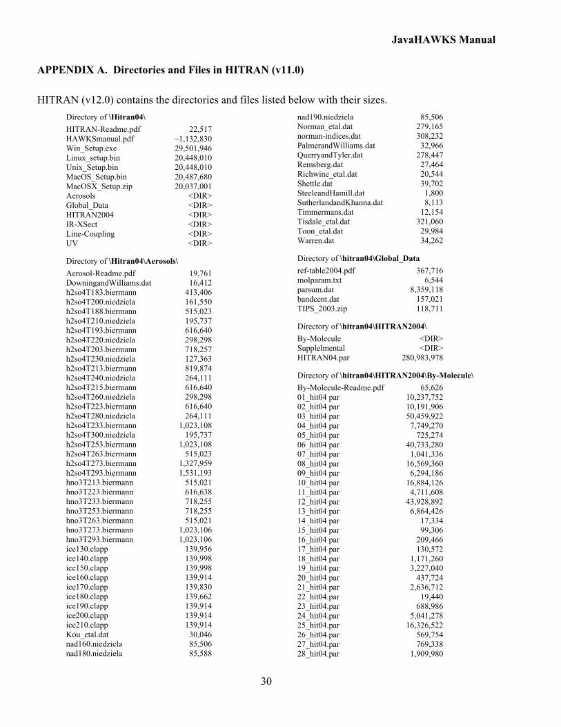
APPENDIX A. Directories and Files in HITRAN (v11.0)
HITRAN (v12.0) contains the directories and files listed below with their sizes. Directory of \Hitran04\ HITRAN-Readme.pdf 22,517 HAWKSmanual.pdf ~1,132,830 Win_Setup.exe 29,501,946 Linux_setup.bin 20,448,010 Unix_Setup.bin 20,448,010 MacOS_Setup.bin 20,487,680 MacOSX_Setup.zip 20,037,001 Aerosols <DIR> Global_Data <DIR> HITRAN2004 <DIR> IR-XSect <DIR> Line-Coupling <DIR> UV <DIR>
Directory of \Hitran04\Aerosols\ Aerosol-Readme.pdf 19,761 DowningandWilliams.dat 16,412 h2so4T183.biermann 413,406 h2so4T200.niedziela 161,550 h2so4T188.biermann 515,023 h2so4T210.niedziela 195,737 h2so4T193.biermann 616,640 h2so4T220.niedziela 298,298 h2so4T203.biermann 718,257 h2so4T230.niedziela 127,363 h2so4T213.biermann 819,874 h2so4T240.niedziela 264,111 h2so4T215.biermann 616,640 h2so4T260.niedziela 298,298 h2so4T223.biermann 616,640 h2so4T280.niedziela 264,111 h2so4T233.biermann 1,023,108 h2so4T300.niedziela 195,737 h2so4T253.biermann 1,023,108 h2so4T263.biermann 515,023 h2so4T273.biermann 1,327,959 h2so4T293.biermann 1,531,193 hno3T213.biermann 515,021 hno3T223.biermann 616,638 hno3T233.biermann 718,255 hno3T253.biermann 718,255 hno3T263.biermann 515,021 hno3T273.biermann 1,023,106 hno3T293.biermann 1,023,106 ice130.clapp 139,956 ice140.clapp 139,998 ice150.clapp 139,998 ice160.clapp 139,914 ice170.clapp 139,830 ice180.clapp 139,662 ice190.clapp 139,914 ice200.clapp 139,914 ice210.clapp 139,914 Kou_etal.dat 30,046 nad160.niedziela 85,506 nad180.niedziela 85,588
nad190.niedziela 85,506 Norman_etal.dat 279,165 norman-indices.dat 308,232 PalmerandWilliams.dat 32,966 QuerryandTyler.dat 278,447 Remsberg.dat 27,464 Richwine_etal.dat 20,544 Shettle.dat 39,702 SteeleandHamill.dat 1,800 SutherlandandKhanna.dat 8,113 Timmermans.dat 12,154 Tisdale_etal.dat 321,060 Toon_etal.dat 29,984 Warren.dat 34,262
Directory of \hitran04\Global_Data ref-table2004.pdf 367,716 molparam.txt 6,544 parsum.dat 8,359,118 bandcent.dat 157,021 TIPS_2003.zip 118,711
Directory of \hitran04\HITRAN2004\ By-Molecule <DIR> Supplelmental <DIR> HITRAN04.par 280,983,978
Directory of \hitran04\HITRAN2004\By-Molecule\ By-Molecule-Readme.pdf 65,626 01_hit04 par 10,237,752 02_hit04 par 10,191,906 03_hit04 par 50,459,922 04_hit04 par 7,749,270 05_hit04 par 725,274 06_hit04 par 40,733,280 07_hit04 par 1,041,336 08_hit04 par 16,569,360 09_hit04 par 6,294,186 10_hit04 par 16,884,126 11_hit04 par 4,711,608 12_hit04 par 43,928,892 13_hit04 par 6,864,426 14_hit04 par 17,334 15_hit04 par 99,306 16_hit04 par 209,466 17_hit04 par 130,572 18_hit04 par 1,171,260 19_hit04 par 3,227,040 20_hit04 par 437,724 21_hit04 par 2,636,712 22_hit04.par 19,440 23_hit04.par 688,986 24_hit04.par 5,041,278 25_hit04.par 16,326,522 26_hit04.par 569,754 27_hit04.par 769,338 28_hit04.par 1,909,980

JavaHAWKS Manual
31
29_hit04.par 11,437,362 31_hit04.par 3,367,656 32_hit04.par 4,018,896 33_hit04.par 6,286,248 34_hit04.par 324 36_hit04.par 195,372 37_hit04.par 705,996 38_hit04.par 2,102,436 39_hit04.par 3,223,638
Directory of \hitran04\HITRAN2004\Supplemental\ 30_hit04.par 3,709,962 35_hit04.par 5,216,238
Directory of \hitran04\IR-XSect\ IRCrossSection-Readme.pdf 59,383 C2F6_IR00.xsc 15,598,934 CCl4_IR00.xsc 2,018,175 CFC-11_IR00.xsc 16,717,448 CFC-113_IR00.xsc 55,692 CFC-114_IR00.xsc 1,496,952 CFC-115_IR00.xsc 777,852 CFC-12_IR00.xsc 21,401,118 CFC-13_IR01.xsc 745,414 CFC-14_IR01.xsc 3,898,920 ClONO2_IR04.xsc 23,732,873 HCFC-123_IR00.xsc 1,868,640 HCFC-124_IR00.xsc 669,629 HCFC-141b_IR00.xsc 1,920,354 HCFC-142b_IR00.xsc 1,984,920 HCFC-21_IR00.xsc 51,306 HCFC-22_IR01.xsc 13,926,811 HCFC-225ca_IR00.xsc 2,060,502 HCFC-225cb_IR00.xsc 2,346,000 HFC-125_IR00.xsc 592,824 HFC-134_IR00.xsc 6,703,434 HFC-134a_IR00.xsc 19,833,114 HFC-143a_IR00.xsc 4,572,846 HFC-152a_IR00.xsc 1,707,582 HFC-32_IR00.xsc 3,813,440 HNO4_IR04.xsc 204,879 N2O5_IR04.xsc 889,440 SF5cf3_IR04.xsc 1,347,810 SF6_IR00.xsc 1,328,960 Supplemental <DIR>
Directory of \hitran04\IR-XSect\Supplemental CFC-11-92_IR00.xsc 319,464 CFC-12-92_IR00.xsc 690,336 ClONO2-96_IR00.xsc 73,950
Directory of \hitran04\Line-Coupling\CO2\ Data_Q <DIR> Soft_Q <DIR> Test_Q <DIR> LineCoupling-Readme.txt 43,511
Directory of \hitran04\UV Line-by-line <DIR> Cross-sections <DIR>
Directory of \hitran04\UV\Line-by-line 07_UV04.par 1,785,240 13_UV04.par 174,798
Directory of \hitran04\UV\Cross-sections BrO_UV04.xsc 110,224 H2CO-UV04.xsc 925,836 N2O-UV00.xsc 143,230 NO2-UV00.xsc 571,264 NO3_UV04.xsc 176,266 O2-O2_UV04.xsc 154,960 O3-UV04.xsc 356,676 OClO_UV04.xsc 1,387,768 SO2-UV00.xsc 2,377,764
JavaHAWKS Manual
32
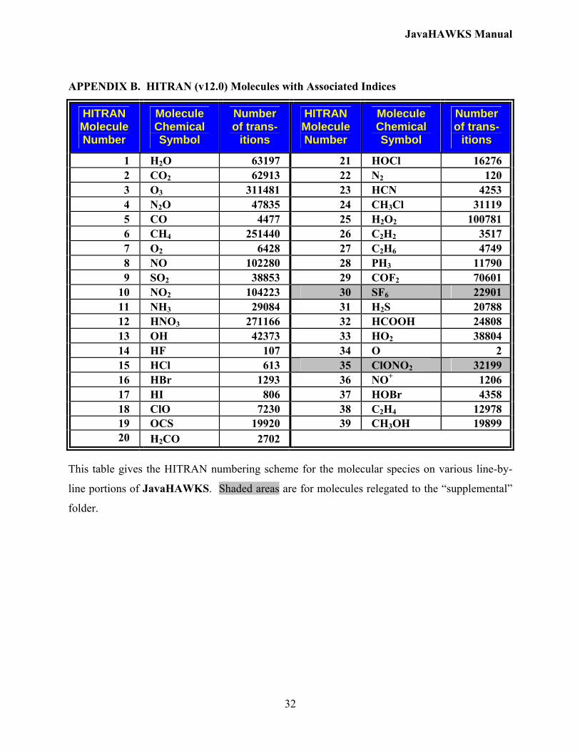
APPENDIX B. HITRAN (v12.0) Molecules with Associated Indices
HITRAN Molecule Number
Molecule Chemical Symbol
Number of trans-
itions
HITRAN Molecule Number
Molecule Chemical Symbol
Number of trans-
itions
1 H2O 63197 21 HOCl 16276 2 CO2 62913 22 N2 120 3 O3 311481 23 HCN 4253 4 N2O 47835 24 CH3Cl 31119 5 CO 4477 25 H2O2 100781 6 CH4 251440 26 C2H2 3517 7 O2 6428 27 C2H6 4749 8 NO 102280 28 PH3 11790 9 SO2 38853 29 COF2 70601
10 NO2 104223 30 SF6 22901 11 NH3 29084 31 H2S 20788 12 HNO3 271166 32 HCOOH 24808 13 OH 42373 33 HO2 38804 14 HF 107 34 O 2 15 HCl 613 35 ClONO2 32199 16 HBr 1293 36 NO+ 1206 17 HI 806 37 HOBr 4358 18 ClO 7230 38 C2H4 12978 19 OCS 19920 39 CH3OH 19899 20 H2CO 2702
This table gives the HITRAN numbering scheme for the molecular species on various line-by-
line portions of JavaHAWKS. Shaded areas are for molecules relegated to the “supplemental”
folder.
JavaHAWKS Manual
33
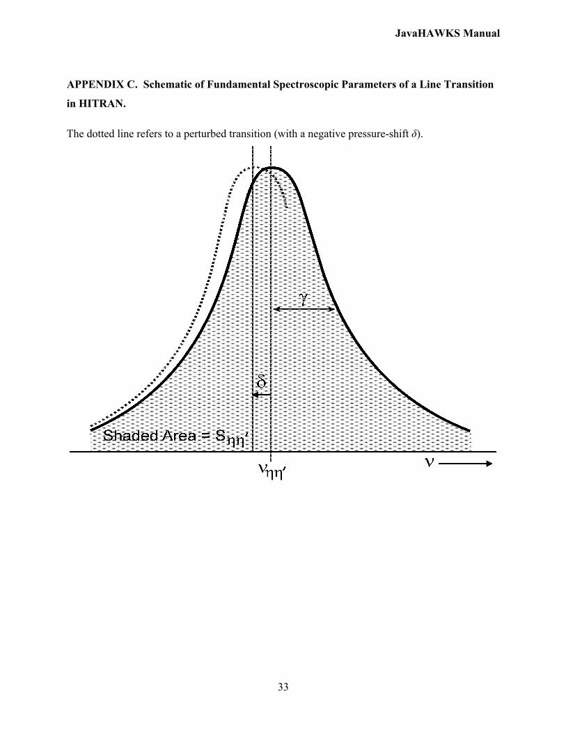
APPENDIX C. Schematic of Fundamental Spectroscopic Parameters of a Line Transition
in HITRAN.
The dotted line refers to a perturbed transition (with a negative pressure-shift δ).

JavaHAWKS Manual
34
APPENDIX D. Formats for Line-by-line Parameters and Cross-section Headers
“1986-2001” line parameter format:
M I S R air self E” n iv’ iv” q’ q” ier iref I2 I F12.6 E10.3 E10.3 F5.4 F5.4 F10.4 F4.2 F8.6 I3 I3 A9 A9 3I13I2
10 20 30 40 50 60 70 80 90
“2002+” line parameter format: M I
S A air self E” n v’ v” Q’ Q” ierr iref * g’ g” I2 I1 F12.6 E10.3 E10.3 F5.4 F5.4 F10.4 F4.2 F8.6 A15 A15 A15 A15 6I1 6I2 A1 F7.1 F7.1
10 20 30 40 50 60 70 80 90 100 110 120 130 140 150 160
Note: v’ and v” are ASCII representations of upper and lower global quanta; * is flag for line coupling; g’ and g” are upper and lower statistical weights. “2000” Cross-section Header format:
Chemical symbol Wavenumber No. Temp Press Max Res. Common Name Not Re Min Max Pts. [K] [Torr] X-section used
BrNo
20 10 10 7 7 6 10 5 15 4 3 3
10 20 30 40 50 60 70 80 90
Note: Chemical Symbol is right adjusted; Res. is resolution in cm-1 for FTS measurements, and in milli-Angstroms for grating measurements in the UV (xxxmÅ), and Br indicates any broadening gas, such as air.
JavaHAWKS Manual
35
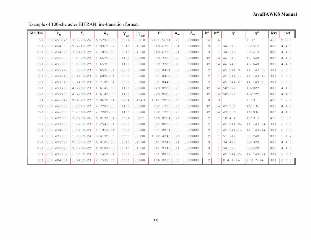
Example of 100-character HITRAN line-transition format.
Mol/Iso ij Sij Rij air self E" nair δair iv' iv" q' q" ierr iref
21 800.451076 3.197E-26 6.579E-05 .0676 .0818 2481.5624 .78 .000000 14 6 P 37 465 2 2 1
291 800.454690 9.724E-22 1.896E-02 .0845 .1750 369.6303 .94 .000000 9 1 341619 331519 000 4 4 1
291 800.454690 3.242E-22 2.107E-03 .0845 .1750 369.6303 .94 .000000 9 1 341519 331419 000 4 4 1
121 800.455380 1.037E-22 1.657E-03 .1100 .0000 530.3300 .75 .000000 32 14 46 640 45 540 000 4 4 1
121 800.455380 1.037E-22 1.657E-03 .1100 .0000 530.3300 .75 .000000 32 14 46 740 45 640 000 4 4 1
101 800.456743 1.680E-23 1.659E-04 .0670 .0000 851.0494 .50 .000000 2 1 45 244 0- 44 143 0- 301 6 6 1
101 800.457045 1.710E-23 1.689E-04 .0670 .0000 851.0469 .50 .000000 2 1 45 244 1- 44 143 1- 301 6 6 1
101 800.457310 1.740E-23 1.718E-04 .0670 .0000 851.0442 .50 .000000 2 1 45 244 2- 44 143 2- 301 6 6 1
121 800.457760 4.726E-23 4.614E-03 .1100 .0000 920.0900 .75 .000000 32 14 502922 492822 000 4 4 1
121 800.457760 4.726E-23 4.614E-03 .1100 .0000 920.0900 .75 .000000 32 14 502922 492722 000 4 4 1
24 800.465942 9.792E-27 6.063E-04 .0754 .1043 1341.2052 .69 .000000 8 3 R 13 425 2 2 1
121 800.466160 1.061E-22 2.720E-03 .1100 .0000 632.1200 .75 .000000 32 14 471236 461136 000 4 4 1
121 800.466160 1.061E-22 2.720E-03 .1100 .0000 632.1200 .75 .000000 32 14 471136 461036 000 4 4 1
35 800.472900 3.878E-26 6.919E-04 .0686 .0871 629.0354 .76 .000000 2 1 1814 4 1713 5 455 5 5 1
101 800.473083 1.270E-23 1.254E-04 .0670 .0000 851.0095 .50 .000000 2 1 45 244 0+ 44 143 0+ 301 6 6 1
101 800.474860 1.210E-23 1.195E-04 .0670 .0000 851.0064 .50 .000000 2 1 45 244-1+ 44 143-1+ 301 6 6 1
31 800.475500 1.680E-24 3.617E-05 .0653 .0890 1092.4340 .76 .000000 2 1 51 547 50 248 002 1 1 2
291 800.476220 9.597E-22 6.010E-03 .0845 .1750 361.9747 .94 .000000 9 1 341420 331320 000 4 4 1
291 800.476220 3.199E-22 6.010E-03 .0845 .1750 361.9747 .94 .000000 9 1 341520 331420 000 4 4 1
101 800.476937 1.160E-23 1.145E-04 .0670 .0000 851.0037 .50 .000000 2 1 45 244-2+ 44 143-2+ 301 6 6 1
101 800.484334 1.740E-23 2.153E-05 .0670 .0000 106.0760 .50 .000000 2 1 8 4 4-1+ 9 3 7-1+ 301 6 6 1
JavaHAWKS Manual
36
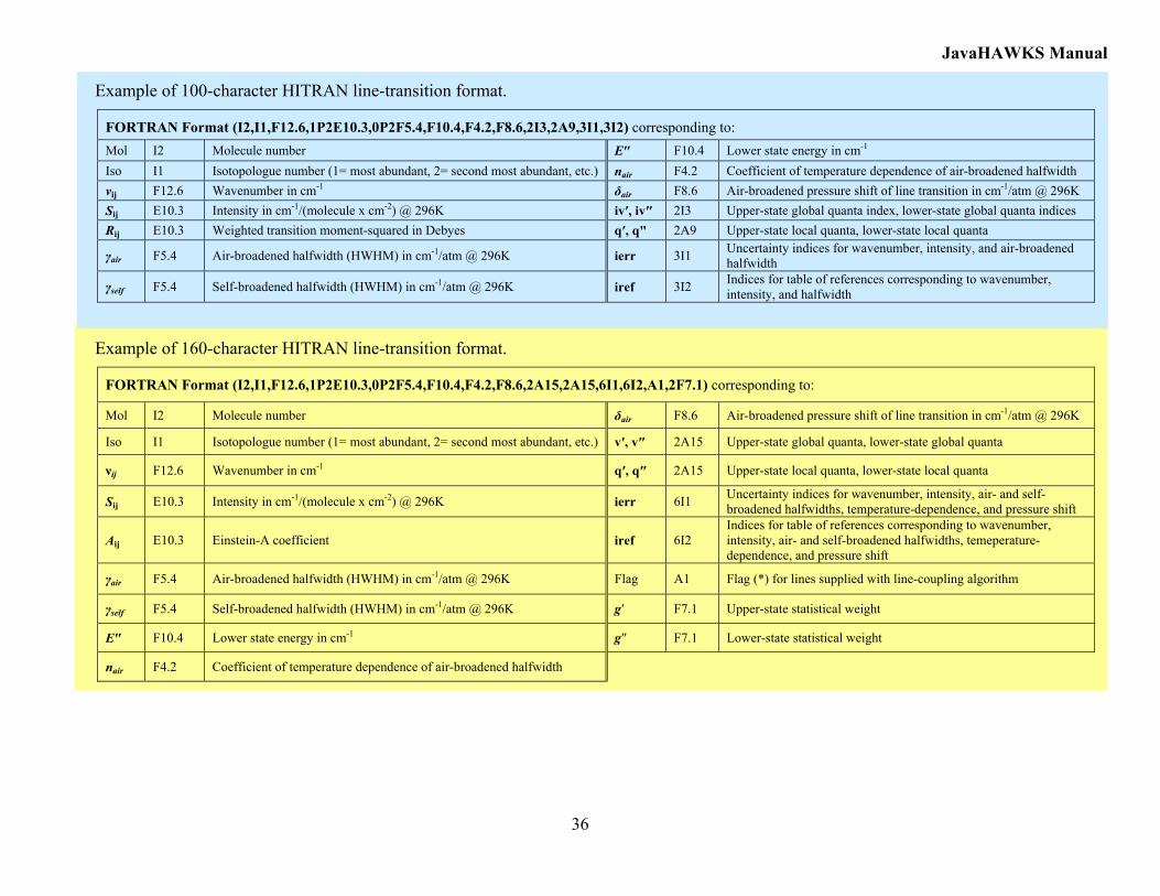
Example of 100-character HITRAN line-transition format.
FORTRAN Format (I2,I1,F12.6,1P2E10.3,0P2F5.4,F10.4,F4.2,F8.6,2I3,2A9,3I1,3I2) corresponding to: Mol I2 Molecule number E″ F10.4 Lower state energy in cm-1 Iso I1 Isotopologue number (1= most abundant, 2= second most abundant, etc.) nair F4.2 Coefficient of temperature dependence of air-broadened halfwidth νij F12.6 Wavenumber in cm-1 δair F8.6 Air-broadened pressure shift of line transition in cm-1/atm @ 296K Sij E10.3 Intensity in cm-1/(molecule x cm-2) @ 296K iv′, iv″ 2I3 Upper-state global quanta index, lower-state global quanta indices Rij E10.3 Weighted transition moment-squared in Debyes q′, q" 2A9 Upper-state local quanta, lower-state local quanta γair F5.4 Air-broadened halfwidth (HWHM) in cm-1/atm @ 296K ierr 3I1 Uncertainty indices for wavenumber, intensity, and air-broadened
halfwidth γself F5.4 Self-broadened halfwidth (HWHM) in cm-1/atm @ 296K iref 3I2 Indices for table of references corresponding to wavenumber,
intensity, and halfwidth
Example of 160-character HITRAN line-transition format.
FORTRAN Format (I2,I1,F12.6,1P2E10.3,0P2F5.4,F10.4,F4.2,F8.6,2A15,2A15,6I1,6I2,A1,2F7.1) corresponding to:
Mol I2 Molecule number δair F8.6 Air-broadened pressure shift of line transition in cm-1/atm @ 296K
Iso I1 Isotopologue number (1= most abundant, 2= second most abundant, etc.) v′, v″ 2A15 Upper-state global quanta, lower-state global quanta
νij F12.6 Wavenumber in cm-1 q′, q″ 2A15 Upper-state local quanta, lower-state local quanta
Sij E10.3 Intensity in cm-1/(molecule x cm-2) @ 296K ierr 6I1 Uncertainty indices for wavenumber, intensity, air- and self-broadened halfwidths, temperature-dependence, and pressure shift
Aij E10.3 Einstein-A coefficient iref 6I2 Indices for table of references corresponding to wavenumber, intensity, air- and self-broadened halfwidths, temeperature-dependence, and pressure shift
γair F5.4 Air-broadened halfwidth (HWHM) in cm-1/atm @ 296K Flag A1 Flag (*) for lines supplied with line-coupling algorithm
γself F5.4 Self-broadened halfwidth (HWHM) in cm-1/atm @ 296K g′ F7.1 Upper-state statistical weight
E″ F10.4 Lower state energy in cm-1 g″ F7.1 Lower-state statistical weight
nair F4.2 Coefficient of temperature dependence of air-broadened halfwidth
Related Documents


