Haroon Mumtaz & Katerina Petrova - QMUL

Changing impact of shocks: a time-varying proxy SVAR approach Haroon Mumtaz & Katerina Petrova

Working paper No. 875 November 2018 ISSN1473-0278

School of Economics and Finance

Changing impact of shocks: a time-varying proxy SVAR approach

Haroon Mumtaz∗ Katerina Petrova†

November 7, 2018

Abstract

In this paper we extend the Bayesian Proxy VAR to incorporate time variation in the para-

meters. A Gibbs sampling algorithm is provided to approximate the posterior distributions of

the model’s parameters. Using the proposed algorithm, we estimate the time-varying effects of

taxation shocks in the US and show that there is limited evidence for a structural change in the

tax multiplier.

Key words: Time-Varying parameters, Stochastic volatility, Proxy VAR, tax shocks

JEL codes: C2,C11, E3

1 Introduction

Temporal changes in macroeconomic dynamics and evolution in the propagation of economic shocks

have been documented in numerous recent studies. In their seminal paper, Cogley and Sargent

(2005) introduce a vector autoregression (VAR) with time-varying parameters and stochastic volatil-

ity (TVP-VAR) and provide evidence supporting shifts in the persistence and volatility of key US

macroeconomic variables. Their model was extended by Primiceri (2005) who also allowed the

∗Queen Mary University London. Email: [email protected]†University of St. Andrews, Email: [email protected]

1

contemporaneous coeffi cients of the VAR model to change over time thus allowing these models to

be used for structural analysis. For example, using this model Benati and Mumtaz (2007) identify

demand and supply shocks via sign restrictions to investigate the causes of the ‘Great Moderation’

in the US. Similarly, Baumeister and Peersman (2013) identify oil supply and demand shocks using

sign restrictions and show that the price elasticity of oil demand in the US has declined over time.

Gali and Gambetti (2009) employ TVP-VARs with long-run restrictions to investigate changes in

US macroeconomic dynamics. Canova and Forero (2015) provide a general algorithm to estimate

TVP-VARs when the shocks are identified via non-recursive identification schemes.

In parallel to this literature on TVP-VARs, the methods used for shock identification in VAR

models have also seen rapid development. An approach that has gained popularity in recent empir-

ical applications is the identification of shocks by using external instruments. This ‘proxy SVAR’

model was introduced by Mertens and Ravn (2013) and Stock and Watson (2008) and differs from

standard identification methods because the contemporaneous impulse response is estimated using

an instrumental variable procedure where the instrument is an exogenous proxy for the shock of

interest, usually constructed via a narrative approach. This reliance on external information re-

duces the number of (possibly controversial) restrictions needed to identify the contemporaneous

impulse response. As the proxy is used as an instrument and not an endogenous variable directly

in the VAR, the effects of measurement error in the proxy can be alleviated. This feature of the

model to combine SVARs with a more narrative approach to estimating causal effects is the key

reason behind the increased popularity of proxy SVAR models in applied work.

In this paper, we propose an algorithm for the estimation of proxy SVAR models when the

parameters of the model are allowed to vary over time, therefore extending the range of methods

for time-varying SVARs described in Canova and Forero (2015). We provide a Gibbs sampling

algorithm to approximate the posterior distributions of the parameters. Our estimation procedure

2

extends the Bayesian MCMC algorithm of Caldara and Herbst (2016) for fixed coeffi cient proxy

SVAR models, by casting it in state space, and applying a ‘state of the art’particle Gibbs algorithm

to filter through the parameter time variation in the resulting nonlinear state space. We design a

small simulation exercise to study the finite sample properties of our proposed algorithm showing

that it displays a satisfactory performance.

Using the proposed model, we investigate the effects of tax shocks on the US economy and

whether these effects have changed over time. To identify the tax shocks we use the narrative

measure proposed by Mertens and Ravn (2012) as an instrument. Our results suggest that the

response of GDP to a tax shock has declined over time but this mainly reflects a decline in the

volatility of the shock rather than a structural change in the fundamental transmission mechanism

of the shock.

The remainder of the paper is organised as follows. Section 2 presents the proxy SVAR model

with time-varying parameters. Section 3 describes the particle Gibbs algorithm and provides a

small Monte Carlo exercise to evaluate the performance of the proposed algorithm. Finally, Section

4 contains our empirical analysis on tax shocks in the US, and Section 5 includes some concluding

remarks.

2 The time-varying proxy SVAR

We consider the following Gaussian VAR model with time-varying parameters:

Yt = BtXt + ut, ut = Σ1/2t εt, εt ∼ N (0, IN ) (1)

where Yt is a N × 1 matrix of endogenous variables, Xt = [Y ′t−1, .., Y′t−P , 1]′ is (NP + 1) × 1

matrix of regressors in each equation and Bt denotes the N × (NP + 1) matrix of coeffi cients

3

Bt = [B1t, ..., BPt, ct]. This VAR model features time-varying autoregressive coeffi cients Bt, where

we follow the literature in assuming that the evolution of the N (NP + 1)× 1 vector bt := vec (B′t)

is described through a random walk transition equation:

bt = bt−1 +Q1/2b ηbt , ηbt ∼ N

(0, IN(NP+1)

), (2)

where Qb is assumed to be diagonal. The time-varying covariance matrix of the reduced form

residuals ut can be written as:

Σt = (Atq) (Atq)′ (3)

where At is a lower triangular matrix with time-varying elements, and q is an element of the family

of orthogonal matrices of size N, satisfying q′q = IN . By considering all possible values of q, the

matrix Atq spans the space of all possible contemporaneous matrices; a result which follows from

the QR decomposition of a square matrix.

Next, we decompose At as:

At = AtH1/2t (4)

where At is a lower triangular matrix with diagonal elements equal to one and Ht is diagonal.

Following Primiceri (2005), we model the evolution of the unrestricted elements of At (where we

donote by the vector at the N (N − 1) /2 × 1 elements below the subdiagonal of At) as random

walks:

αt = αt−1 +Q1/2a ηat , ηat ∼ N(0, IN(N−1)/2

). (5)

Finally, we assume that the diagonal elements of Ht (summarised in an N × 1 vector ht ) evolve as

4

geometric random walks:

lnht = lnht−1 +Q1/2h ηht , ηht ∼ N (0, IN ) . (6)

2.1 Identification of shocks

The structural shocks of the VAR model εt are defined as

εt = A−10,tut, (7)

where A0,t = Atq. We assume, without loss of generality, that we interested in identifying the

first shock ε1t in the N × 1 vector of shocks εt = [ε1t, ε·t], where ε·t contains the remaining N − 1

elements in εt. To do this, we employ an instrument mt described by the following equation:

mt = βε1t + σvt, vt ∼ N (0, 1) (8)

where E (vtεt) = 0. The instrument is assumed to be relevant (β 6= 0) and uncorrelated with other

structural shocks (E (mtε·t) = 0). As discussed in Caldara and Herbst (2016), the relevance of the

instrument can be judged by calculating the reliability statistic of Mertens and Ravn (2013) which

is defined as the squared correlation between mt and ε1t:

ρ =β2

β2 + σ2(9)

5

While we write equation 8 as a fixed coeffi cient model in the benchmark case, our procedure easily

allows the extension to a time-varying β and σ2. For example one can assume that:

βt = βt−1 + σβnβt , nβt ∼ N (0, 1) (10)

lnσ2t = lnσ2t−1 + σσnσt , nσt ∼ N (0, 1) (11)

This extended formulation would also allow the reliability statistic to change over time.

2.1.1 The likelihood function and the role of the instrument

The covariance between the reduced form residuals and the instrument can be defined by:

ut

mt

|Lt ∼ N (0, LtL′t) , Lt =

Atq 0

b σ

(12)

where b is a 1×N vector b =

[β 0 . 0

], since

ut

mt

= Lt

εt

vt

.

To consider the role of the instrument we follow Caldara and Herbst (2016) and factor the likelihood

of the model as:

p (Yt,mt|Ξ) = p (Yt|Ξ) p (mt|Yt,Ξ) (13)

where Ξ denotes all parameters and states of the model. Given the conditional normality assumption

in equation 12, the conditional density p (mt|Yt,Ξ) is also normal with mean µt = βq′1A−1t ut and

variance s = σ2, where q1 is the first column of q.

6

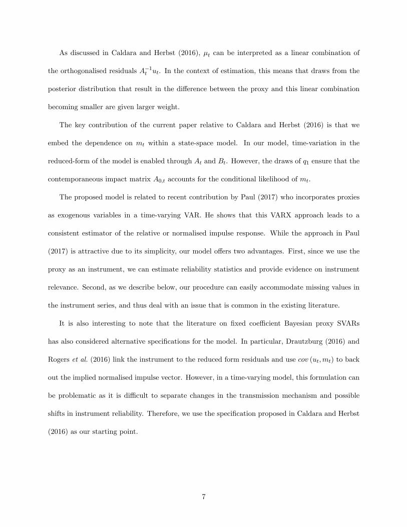
As discussed in Caldara and Herbst (2016), µt can be interpreted as a linear combination of

the orthogonalised residuals A−1t ut. In the context of estimation, this means that draws from the

posterior distribution that result in the difference between the proxy and this linear combination

becoming smaller are given larger weight.

The key contribution of the current paper relative to Caldara and Herbst (2016) is that we

embed the dependence on mt within a state-space model. In our model, time-variation in the

reduced-form of the model is enabled through At and Bt. However, the draws of q1 ensure that the

contemporaneous impact matrix A0,t accounts for the conditional likelihood of mt.

The proposed model is related to recent contribution by Paul (2017) who incorporates proxies

as exogenous variables in a time-varying VAR. He shows that this VARX approach leads to a

consistent estimator of the relative or normalised impulse response. While the approach in Paul

(2017) is attractive due to its simplicity, our model offers two advantages. First, since we use the

proxy as an instrument, we can estimate reliability statistics and provide evidence on instrument

relevance. Second, as we describe below, our procedure can easily accommodate missing values in

the instrument series, and thus deal with an issue that is common in the existing literature.

It is also interesting to note that the literature on fixed coeffi cient Bayesian proxy SVARs

has also considered alternative specifications for the model. In particular, Drautzburg (2016) and

Rogers et al. (2016) link the instrument to the reduced form residuals and use cov (ut,mt) to back

out the implied normalised impulse vector. However, in a time-varying model, this formulation can

be problematic as it is diffi cult to separate changes in the transmission mechanism and possible

shifts in instrument reliability. Therefore, we use the specification proposed in Caldara and Herbst

(2016) as our starting point.

7

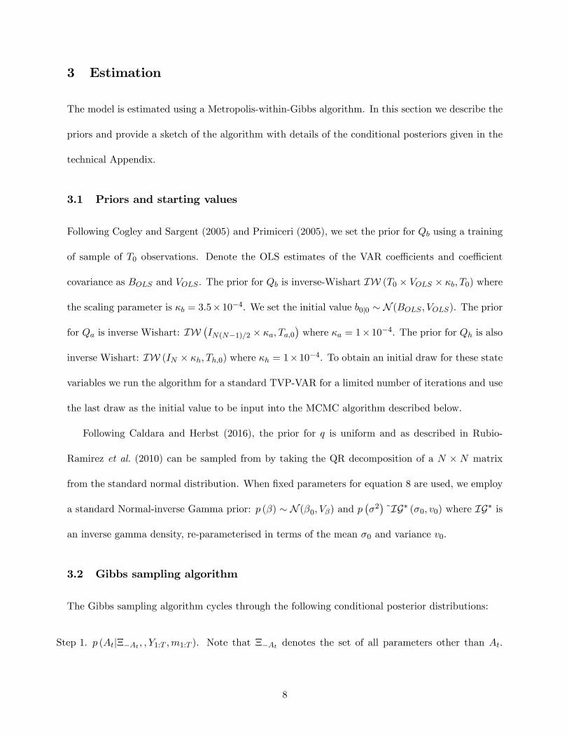
3 Estimation

The model is estimated using a Metropolis-within-Gibbs algorithm. In this section we describe the

priors and provide a sketch of the algorithm with details of the conditional posteriors given in the

technical Appendix.

3.1 Priors and starting values

Following Cogley and Sargent (2005) and Primiceri (2005), we set the prior for Qb using a training

of sample of T0 observations. Denote the OLS estimates of the VAR coeffi cients and coeffi cient

covariance as BOLS and VOLS . The prior for Qb is inverse-Wishart IW (T0 × VOLS × κb, T0) where

the scaling parameter is κb = 3.5×10−4. We set the initial value b0|0 ∼ N (BOLS , VOLS). The prior

for Qa is inverse Wishart: IW(IN(N−1)/2 × κa, Ta,0

)where κa = 1× 10−4. The prior for Qh is also

inverse Wishart: IW (IN × κh, Th,0) where κh = 1×10−4. To obtain an initial draw for these state

variables we run the algorithm for a standard TVP-VAR for a limited number of iterations and use

the last draw as the initial value to be input into the MCMC algorithm described below.

Following Caldara and Herbst (2016), the prior for q is uniform and as described in Rubio-

Ramirez et al. (2010) can be sampled from by taking the QR decomposition of a N × N matrix

from the standard normal distribution. When fixed parameters for equation 8 are used, we employ

a standard Normal-inverse Gamma prior: p (β) ∼ N (β0, Vβ) and p(σ2)

˜IG∗ (σ0, v0) where IG∗ is

an inverse gamma density, re-parameterised in terms of the mean σ0 and variance v0.

3.2 Gibbs sampling algorithm

The Gibbs sampling algorithm cycles through the following conditional posterior distributions:

Step 1. p (At|Ξ−At , , Y1:T ,m1:T ). Note that Ξ−At denotes the set of all parameters other than At.

8

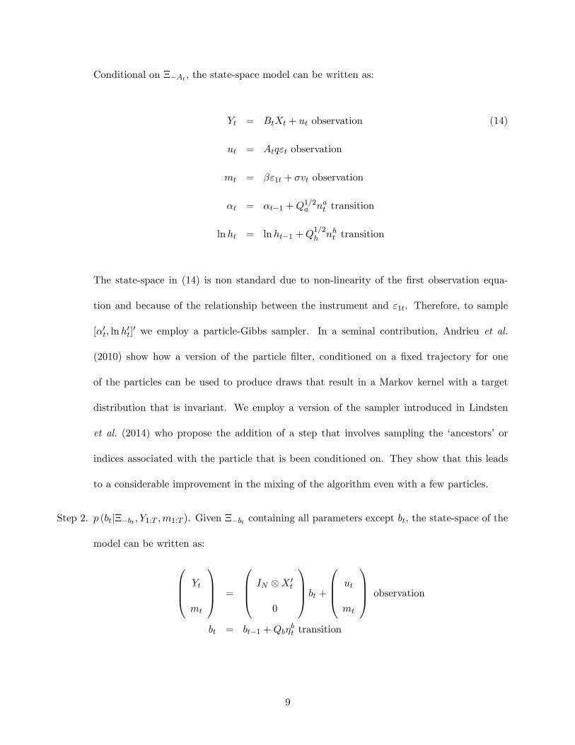
Conditional on Ξ−At , the state-space model can be written as:

Yt = BtXt + ut observation (14)

ut = Atqεt observation

mt = βε1t + σvt observation

αt = αt−1 +Q1/2a nat transition

lnht = lnht−1 +Q1/2h nht transition

The state-space in (14) is non standard due to non-linearity of the first observation equa-

tion and because of the relationship between the instrument and ε1t. Therefore, to sample

[α′t, lnh′t]′ we employ a particle-Gibbs sampler. In a seminal contribution, Andrieu et al.

(2010) show how a version of the particle filter, conditioned on a fixed trajectory for one

of the particles can be used to produce draws that result in a Markov kernel with a target

distribution that is invariant. We employ a version of the sampler introduced in Lindsten

et al. (2014) who propose the addition of a step that involves sampling the ‘ancestors’ or

indices associated with the particle that is been conditioned on. They show that this leads

to a considerable improvement in the mixing of the algorithm even with a few particles.

Step 2. p (bt|Ξ−bt , Y1:T ,m1:T ). Given Ξ−bt containing all parameters except bt, the state-space of the

model can be written as:

Yt

mt

=

IN ⊗X ′t

0

bt +

ut

mt

observation

bt = bt−1 +Qbηbt transition

9

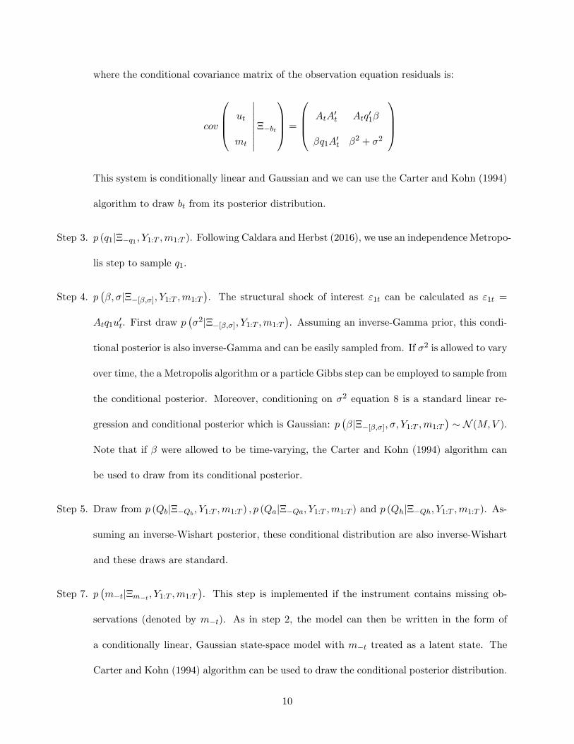
where the conditional covariance matrix of the observation equation residuals is:

cov

ut

mt

∣∣∣∣∣∣∣∣Ξ−bt =

AtA′t Atq

′1β

βq1A′t β2 + σ2

This system is conditionally linear and Gaussian and we can use the Carter and Kohn (1994)

algorithm to draw bt from its posterior distribution.

Step 3. p (q1|Ξ−q1 , Y1:T ,m1:T ). Following Caldara and Herbst (2016), we use an independence Metropo-

lis step to sample q1.

Step 4. p(β, σ|Ξ−[β,σ], Y1:T ,m1:T

). The structural shock of interest ε1t can be calculated as ε1t =

Atq1u′t. First draw p

(σ2|Ξ−[β,σ], Y1:T ,m1:T

). Assuming an inverse-Gamma prior, this condi-

tional posterior is also inverse-Gamma and can be easily sampled from. If σ2 is allowed to vary

over time, the a Metropolis algorithm or a particle Gibbs step can be employed to sample from

the conditional posterior. Moreover, conditioning on σ2 equation 8 is a standard linear re-

gression and conditional posterior which is Gaussian: p(β|Ξ−[β,σ], σ, Y1:T ,m1:T

)∼ N (M,V ).

Note that if β were allowed to be time-varying, the Carter and Kohn (1994) algorithm can

be used to draw from its conditional posterior.

Step 5. Draw from p (Qb|Ξ−Qb , Y1:T ,m1:T ) , p (Qa|Ξ−Qa, Y1:T ,m1:T ) and p (Qh|Ξ−Qh, Y1:T ,m1:T ). As-

suming an inverse-Wishart posterior, these conditional distribution are also inverse-Wishart

and these draws are standard.

Step 7. p(m−t|Ξm−t , Y1:T ,m1:T

). This step is implemented if the instrument contains missing ob-

servations (denoted by m−t). As in step 2, the model can then be written in the form of

a conditionally linear, Gaussian state-space model with m−t treated as a latent state. The

Carter and Kohn (1994) algorithm can be used to draw the conditional posterior distribution.

10

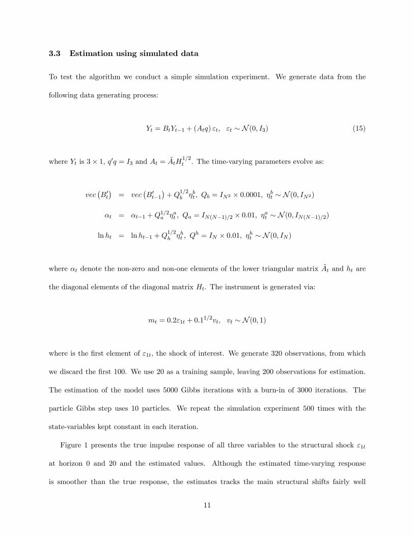
3.3 Estimation using simulated data

To test the algorithm we conduct a simple simulation experiment. We generate data from the

following data generating process:

Yt = BtYt−1 + (Atq) εt, εt ∼ N (0, I3) (15)

where Yt is 3× 1, q′q = I3 and At = AtH1/2t . The time-varying parameters evolve as:

vec(B′t)

= vec(B′t−1

)+Q

1/2b ηbt , Qb = IN2 × 0.0001, ηbt ∼ N (0, IN2)

αt = αt−1 +Q1/2a ηat , Qa = IN(N−1)/2 × 0.01, ηat ∼ N (0, IN(N−1)/2)

lnht = lnht−1 +Q1/2h ηht , Q

h = IN × 0.01, ηht ∼ N (0, IN )

where αt denote the non-zero and non-one elements of the lower triangular matrix At and ht are

the diagonal elements of the diagonal matrix Ht. The instrument is generated via:

mt = 0.2ε1t + 0.11/2vt, vt ∼ N (0, 1)

where is the first element of ε1t, the shock of interest. We generate 320 observations, from which

we discard the first 100. We use 20 as a training sample, leaving 200 observations for estimation.

The estimation of the model uses 5000 Gibbs iterations with a burn-in of 3000 iterations. The

particle Gibbs step uses 10 particles. We repeat the simulation experiment 500 times with the

state-variables kept constant in each iteration.

Figure 1 presents the true impulse response of all three variables to the structural shock ε1t

at horizon 0 and 20 and the estimated values. Although the estimated time-varying response

is smoother than the true response, the estimates tracks the main structural shifts fairly well

11

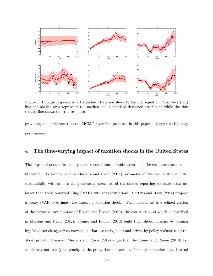
Figure 1: Impulse response to a 1 standard deviation shock to the first equation. The thick (red)line and shaded area represents the median and 1 standard deviation error band while the thin(black) line shows the true response.

providing some evidence that the MCMC algorithm proposed in this paper displays a satisfactory

performance.

4 The time-varying impact of taxation shocks in the United States

The impact of tax shocks on output has received considerable attention in the recent macroeconomic

literature. As pointed out in Mertens and Ravn (2014), estimates of the tax multiplier differ

substantially with studies using narrative measures of tax shocks reporting estimates that are

larger than those obtained using SVARs with zero restrictions. Mertens and Ravn (2014) propose

a proxy SVAR to estimate the impact of taxation shocks. Their instrument is a refined version

of the narrative tax measure of Romer and Romer (2010), the construction of which is described

in Mertens and Ravn (2012). Romer and Romer (2010) build their shock measure by purging

legislated tax changes from movements that are endogenous and driven by policy makers’concerns

about growth. However, Mertens and Ravn (2012) argue that the Romer and Romer (2010) tax

shock may not satisfy exogeneity as the proxy does not account for implementation lags. Instead

12

Mertens and Ravn (2012) propose a proxy based on exogenous tax changes where legislation and

implementation are less than a quarter apart. Using this measure, Mertens and Ravn (2014)

estimate tax multipliers that lie towards the upper end of the range of estimates.

While a number of studies have attempted to pin down the average estimate of taxation shocks,

there is little existing evidence regarding changes in the transmission of this shock across time.

An exception is Perotti (2005) who uses sub-sample estimates of the Blanchard and Perotti (2002)

SVAR and finds some evidence of a decline in the impact of taxation shocks. In contrast, Mertens

and Ravn (2014) show that this sub-sample evidence is much weaker when their proxy VAR is used

to estimate the effects of tax shocks.

In this section, we re-visit this question by using our MCMC algorithm to estimate a time-

varying proxy SVAR with the tax shock identified with the help of the narrative shock measure of

Mertens and Ravn (2012).

4.1 Empirical model, data and priors

We estimate a TVP proxy SVAR(4) model using our MCMC algorithm. The model is

Yt = BtXt + ut

where Xt contains four lags and an intercept Xt = [Y ′t−1, ..., Y′t−4, 1]′ and var (ut|At) = AtAt

′.

The elements of the coeffi cient matrices Bt, and At evolve over time as random walks, subject to

stability condition for Bt. The endogenous variables include (i) real per-capita federal government

revenue (Tt), (ii) real per-capita federal government spending (Gt) , and (iii) real per-capita GDP

(It). As described in the technical Appendix, Government spending is defined as the sum of

federal government consumption and investment. Taxes are calculated as current receipts of the

federal government plus contributions for social insurance less corporate income taxes from Federal

13

Reserve banks. Both variables are deflated by the GDP deflator and divided by total population.

The variables enter the model in log differences and the sample period runs from 1948Q2 to 2016Q2.

Note that the tax shock proxy is only available from 1950Q1 to 2006Q4 and the missing observations

are estimated as additional states in the model.

The prior for Qb is set using OLS estimates of the VAR over a training sample of T0 = 50

observations. The priors for Qa and Qh have prior degrees of freedom of 15 to give some weight

to the prior belief that changes in At are gradual. We set loose priors for the instrument equation

parameters β and σ2 in the benchmark case: p(β) ∼ N (0.1, 1), p(σ2) ∼ IG∗(0.05, 1). We compare

this with an alternative set of priors that incorporates the belief that the instrument is strongly

relevant. Under this prior belief: p(β)˜N(0.15, 10−5) while p(σ2) remains G2(0.05, 1). When setting

the prior for q1, we incorporate the belief that tax increases should reduce output. 1As discussed

in Mertens and Ravn (2014), compared to views on the size of the impact of tax shocks, this belief

on the sign of the impact is relatively uncontroversial.

The MCMC algorithm uses 100,000 replications with a burn-in period of 50,000. Every 10th

remaining draw is used for inference. The particle Gibbs step employs 10 particles. The technical

appendix presents some evidence for convergence of the algorithm.

4.1.1 Empirical Results

Following Caldara and Herbst (2016), we consider the relevance of the tax shock instrument by

calculating the reliability statistic (ρ) of Mertens and Ravn (2013) given in equation 9 above. The

estimated posterior distribution of this statistic under the benchmark prior suggests that within

our TVP setting, reliability of this instrument is lower than that reported in Mertens and Ravn

(2014) for a fixed coeffi cient model. The median estimate of ρ is 0.08, albeit with the 68 percent

1This is implemented by rejecting draws from the candidate density in Step 3 of the estimation algorithm thatfail to satisfy this belief. Rogers et al. (2016) also incorporate inequality restrictions in their application to monetarypolicy.

14

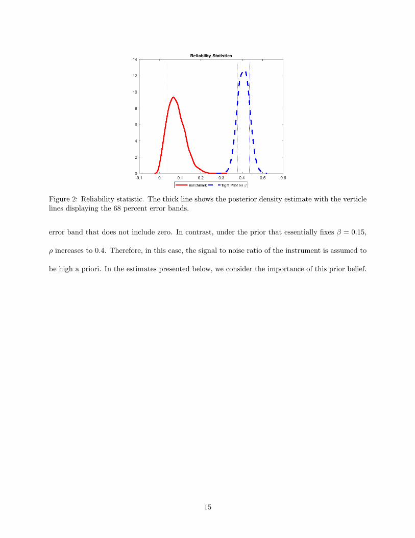
Figure 2: Reliability statistic. The thick line shows the posterior density estimate with the verticlelines displaying the 68 percent error bands.

error band that does not include zero. In contrast, under the prior that essentially fixes β = 0.15,

ρ increases to 0.4. Therefore, in this case, the signal to noise ratio of the instrument is assumed to

be high a priori. In the estimates presented below, we consider the importance of this prior belief.

15

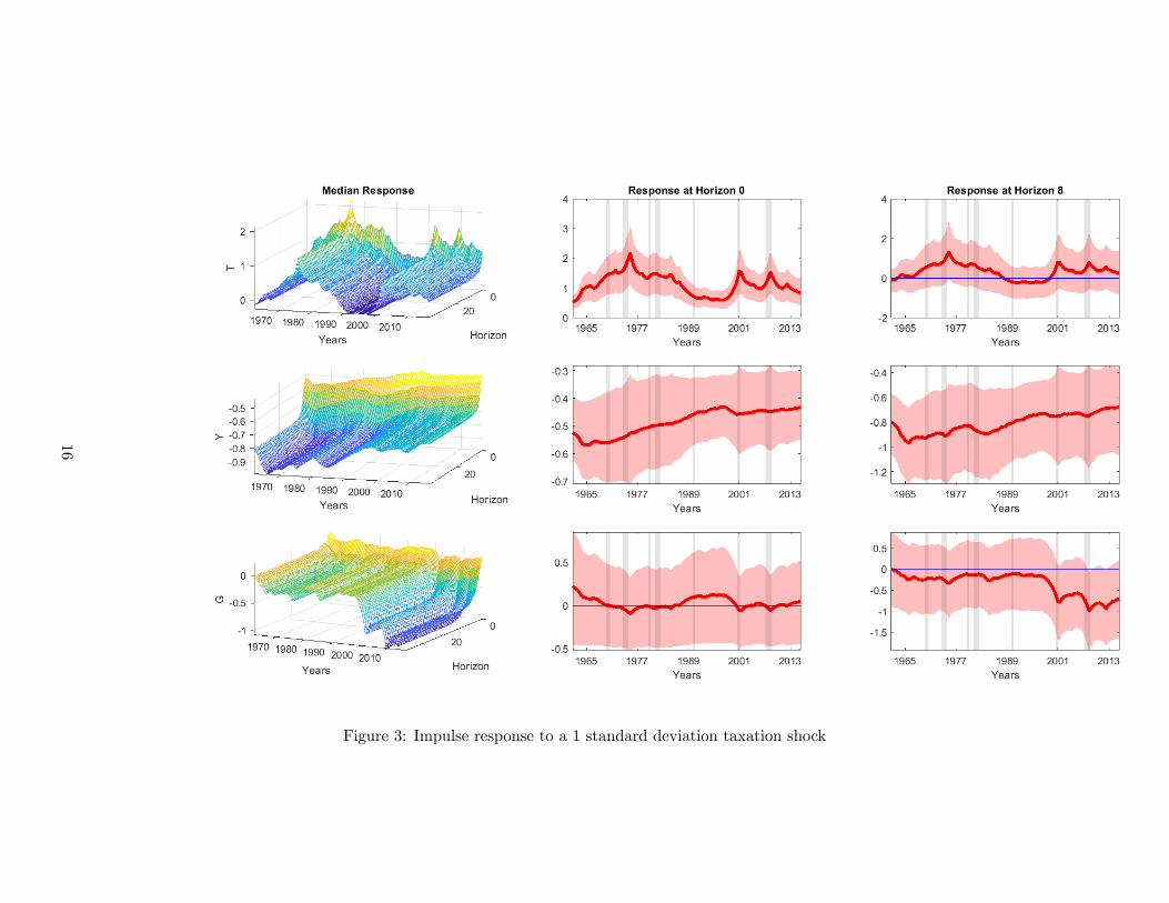
Figure 3: Impulse response to a 1 standard deviation taxation shock

16

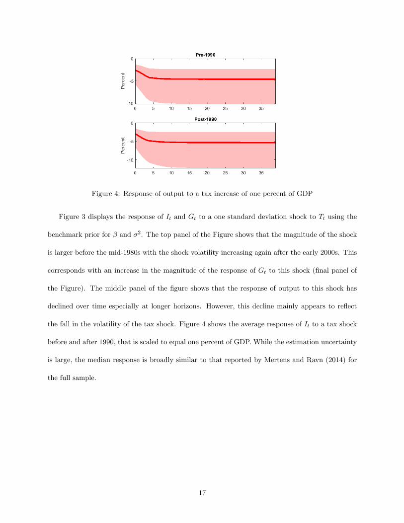
Figure 4: Response of output to a tax increase of one percent of GDP

Figure 3 displays the response of It and Gt to a one standard deviation shock to Tt using the

benchmark prior for β and σ2. The top panel of the Figure shows that the magnitude of the shock

is larger before the mid-1980s with the shock volatility increasing again after the early 2000s. This

corresponds with an increase in the magnitude of the response of Gt to this shock (final panel of

the Figure). The middle panel of the figure shows that the response of output to this shock has

declined over time especially at longer horizons. However, this decline mainly appears to reflect

the fall in the volatility of the tax shock. Figure 4 shows the average response of It to a tax shock

before and after 1990, that is scaled to equal one percent of GDP. While the estimation uncertainty

is large, the median response is broadly similar to that reported by Mertens and Ravn (2014) for

the full sample.

17

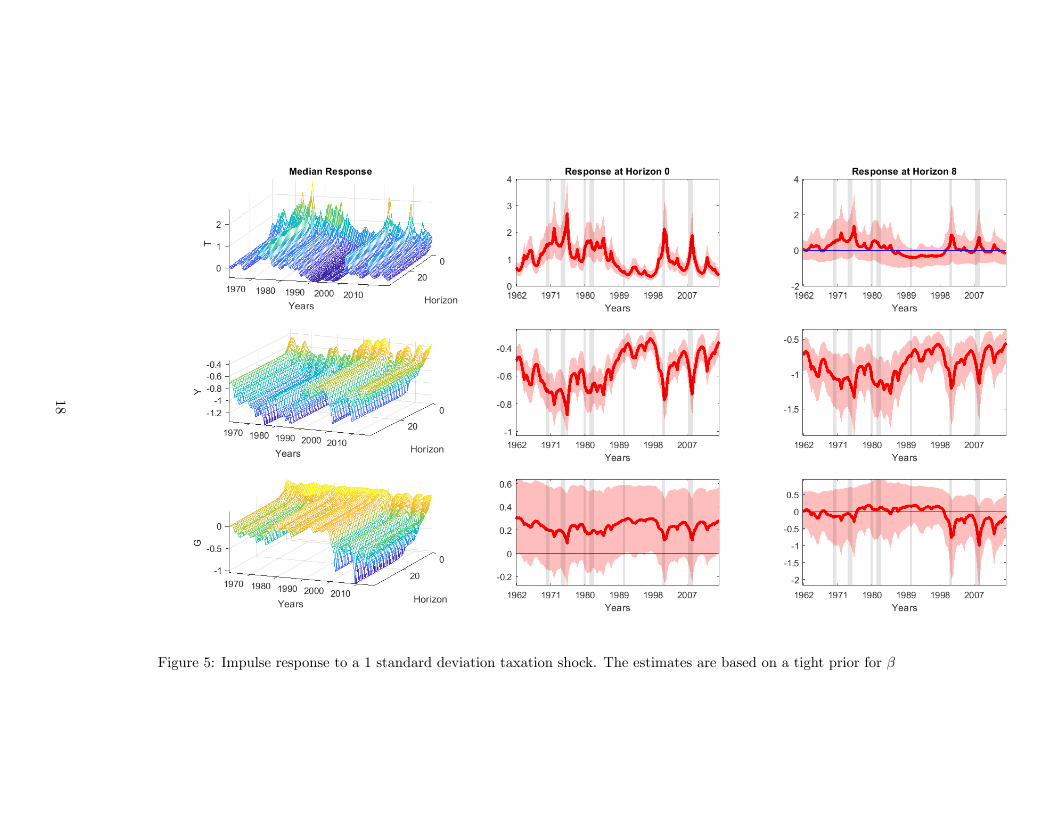
Figure 5: Impulse response to a 1 standard deviation taxation shock. The estimates are based on a tight prior for β

18

Figure 5 considers the impulse response functions when instrument reliability is assumed to

be high a priori. These estimates suggest a number of conclusions. First, the time-variation in

the responses is more pronounced at higher frequencies. In other words, the responses change less

smoothly than in the benchmark case and display more variation in the short-run. Second, the

error bands for the response of output are less wide. This suggests that inference is sharpened

by incorporating a higher signal from the tax instrument. Finally, while these responses are more

volatile through time, the economic conclusions regarding the transmission of the tax shock are

unaltered. Changes in the response of It to this shock largely reflect changes in the volatility of the

tax shock.

5 Conclusion

This paper proposes a time-varying proxy SVAR model that can be used to estimate changes in

the transmission of shocks. We provide a Gibbs sampling algorithm to approximate the posterior

distribution of the parameters. Using a simple simulation experiment, we show that the algorithm

displays a reasonable performance. The proposed model is used to estimate the time-varying

response to tax shocks in the US. Our results suggest that while the volatility of tax shocks has

declined, there is limited evidence to suggest a change in the transmission of this shock to output.

References

Andrieu, Christophe, Arnaud Doucet and Roman Holenstein, 2010, Particle Markov chain Monte

Carlo methods, Journal of the Royal Statistical Society Series B 72(3), 269—342.

Baumeister, Christiane and Gert Peersman, 2013, Time-Varying Effects of Oil Supply Shocks on

the US Economy, American Economic Journal: Macroeconomics 5(4), 1—28.

19

Benati, Luca and Haroon Mumtaz, 2007, U.S. evolving macroeconomic dynamics - a structural

investigation, Working Paper Series 746, European Central Bank.

Blanchard, Olivier and Roberto Perotti, 2002, An Empirical Characterization of the Dynamic

Effects of Changes in Government Spending and Taxes on Output, The Quarterly Journal of

Economics 117(4), 1329—1368.

Caldara, Dario and Edward Herbst, 2016, Monetary Policy, Real Activity, and Credit Spreads:

Evidence from Bayesian Proxy SVARs, Finance and Economics Discussion Series 2016-049,

Board of Governors of the Federal Reserve System (U.S.).

Canova, Fabio and Fernando J. Pérez Forero, 2015, Estimating overidentified, nonrecursive, time

varying coeffi cients structural vector autoregressions, Quantitative Economics 6(2), 359—384.

Carter, C and P Kohn, 1994, On Gibbs sampling for state space models, Biometrika 81, 541—53.

Cogley, Timothy and Thomas J. Sargent, 2005, Drift and Volatilities: Monetary Policies and

Outcomes in the Post WWII U.S, Review of Economic Dynamics 8(2), 262—302.

Drautzburg, Thorsten, 2016, A narrative approach to a fiscal DSGE model,Working Papers 16-11,

Federal Reserve Bank of Philadelphia.

Gali, Jordi and Luca Gambetti, 2009, On the Sources of the Great Moderation, American Economic

Journal: Macroeconomics 1(1), 26—57.

Lindsten, Fredrik, Michael I. Jordan and Thomas B. Schön, 2014, Particle Gibbs with Ancestor

Sampling, Journal of Machine Learning Research 15, 2145—2184.

Mertens, Karel and Morten O. Ravn, 2012, Empirical Evidence on the Aggregate Effects of Antici-

pated and Unanticipated US Tax Policy Shocks, American Economic Journal: Economic Policy

4(2), 145—81.

20

Mertens, Karel and Morten O. Ravn, 2013, The Dynamic Effects of Personal and Corporate Income

Tax Changes in the United States, American Economic Review 103(4), 1212—47.

Mertens, Karel and Morten O. Ravn, 2014, A reconciliation of SVAR and narrative estimates of

tax multipliers, Journal of Monetary Economics 68, S1 —S19.

Paul, Pascal, 2017, The Time-Varying Effect of Monetary Policy on Asset Prices, Working Paper

Series 2017-9, Federal Reserve Bank of San Francisco.

Perotti, Roberto, 2005, Estimating the effects of fiscal policy in OECD countries, Proceedings .

Primiceri, G, 2005, Time varying structural vector autoregressions and monetary policy, The Review

of Economic Studies 72(3), 821—52.

Rogers, John H., Chiara Scotti and Jonathan H. Wright, 2016, Unconventional Monetary Policy and

International Risk Premia, International Finance Discussion Papers 1172, Board of Governors

of the Federal Reserve System (U.S.).

Romer, Christina D. and David H. Romer, 2010, The Macroeconomic Effects of Tax Changes:

Estimates Based on a New Measure of Fiscal Shocks, American Economic Review 100(3), 763—

801.

Rubio-Ramirez, Juan F, Daniel Waggoner and Tao Zha, 2010, Structural Vector Autoregressions:

Theory of Identification and Algorithms for Inference, Review of Economic Studies 77(2), 665—

696.

Stock, James H. and Mark W. Watson, 2008, What’s New in Econometrics- Time Series, Lecture 7,

National Bureau of Economic Research, Inc.

21

This working paper has been produced by the School of Economics and Finance at Queen Mary University of London

Copyright © 2018 Haroon Mumtaz & Katerina Petrova all rights reserved

School of Economics and Finance Queen Mary University of London Mile End RoadLondon E1 4NSTel: +44 (0)20 7882 7356Fax: +44 (0)20 8983 3580Web: www.econ.qmul.ac.uk/research/workingpapers/

School of Economics and Finance