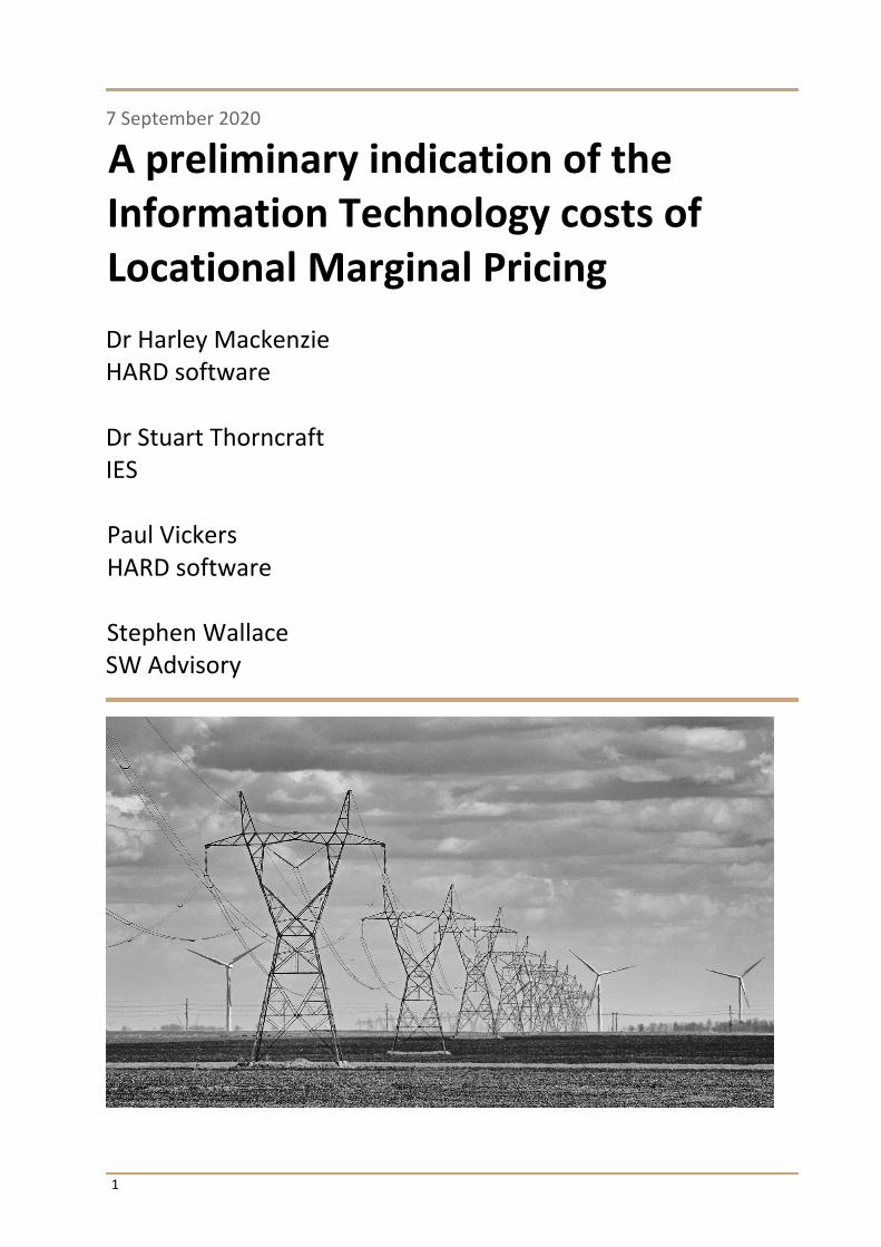
Hard Software - Information Technology costs of nodal pricing

1

7 September 2020

A preliminary indication of the Information Technology costs of Locational Marginal Pricing Dr Harley Mackenzie HARD software Dr Stuart Thorncraft IES Paul Vickers HARD software Stephen Wallace SW Advisory

2

Executive summary

Introduction

The Australian Energy Market Commission (AEMC) contracted HARD software, in association with

SW Advisory and Intelligent Energy Systems, to provide a quick assessment of the impact to the

market operator’s and market participants’ systems associated with implementing Locational

Marginal Pricing (LMP – also referred to as ‘nodal pricing’) and Financial Transmission Rights

(FTRs) within the Australian National Energy Market (NEM).

The purpose of the assessment is to give a view of the likely system’s costs, taking into account

savings and offsets against future required expenditure for the market operator and market

participants.

Given the short time in which to undertake the assessment, the project team based our analysis

on our extensive experience with the implementation of similar market systems for system and

market operators and market participants.

Locational Marginal Price

The locational marginal price is the cost of supplying the next increment of load or the value of

providing the next increment of generation at a specific location (node) on the transmission

network taking into account the market participants’ bids and offers, the physical capabilities of

the transmission system and the need to run the power system in a secure manner. The LMP for

a node and time includes the costs of transmission losses and congestion and the costs of

dispatchable resources (generation, loads and FCAS providers). With modern dispatch and

pricing systems, locational marginal prices (LMPs or nodal prices) are generally computed for

each node (bus) in the transmission network.

LMP Options

The AEMC requested that the authors address the costs of introducing LMP and FTRs to varying

degrees of effectiveness. In particular, the AEMC asked that we look at the following costs:

● an initial estimate of costs to the market operator and participants of introducing LMP

and FTRs, while maintaining the existing regional reference price and loss framework,

3

that is mostly using the current NEMDE framework and producing nodal generator prices

based on constraint costs and continue with a single regional reference price (Option 1:

the base case),

● the incremental costs (relative to the base case) of replacing the regional reference price

with a volume-weighted average price, that is developing locational marginal prices for

all generation and load nodes but with non-dynamic loss factors and the calculation of a

load weighted regional reference price (Option 2), and

● incremental costs (relative to the base case) of introducing a full network model, dynamic

losses and locational marginal prices for loads and generation and the calculation of load

weighted regional prices (Option 3).

Results

The report estimates only the incremental costs associated with the implementation of

Locational Marginal Pricing into the Australian NEM, excluding internal or existing resources that

would already have been deployed by both AEMO and the market participants regardless of the

implementation of Locational Marginal Pricing.

Given the short time in which to undertake the assessment of costs, the project team based our

analysis on our experience with the implementation of similar market systems for system and

market operators and market participants.

The following table is a summary of incremental market costs associated with each of the three

LMP options (in 2020 AUD nominal currency terms):

Option 1 Option 2 Option 3

Upfront Ongoing Upfront Ongoing Upfront Ongoing

AEMO $8,180,000 $2,710,000 $15,050,000 $3,120,000 $23,550,000 $4,450,000

Participant $31,500,000 $0 $37,850,000 $0 $37,850,000 $0

Total $39,680,000 $2,710,000 $52,900,000 $3,120,000 $61,390,000 $4,450,000

Table 1 Total increased market costs associated with each LMP option.

The resulting NPVs of the costs for the 20-year period from 2021-40 expressed in Real 2020 AUD

currency (rounded up to the nearest 1 million AUD) using 5% real discount rate (7% nominal

discount rate and 2% inflation) are:

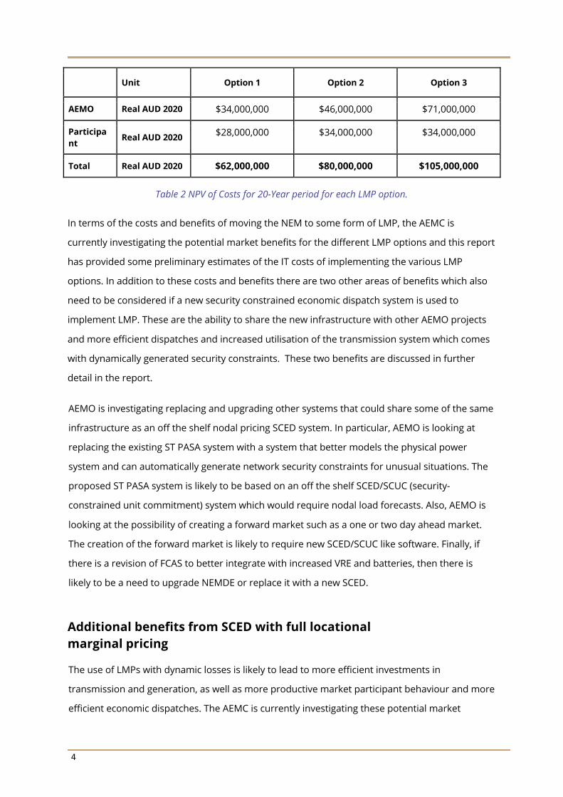
4

Unit Option 1 Option 2 Option 3

AEMO Real AUD 2020 $34,000,000 $46,000,000 $71,000,000

Participant

Real AUD 2020 $28,000,000 $34,000,000 $34,000,000

Total Real AUD 2020 $62,000,000 $80,000,000 $105,000,000

Table 2 NPV of Costs for 20-Year period for each LMP option.

In terms of the costs and benefits of moving the NEM to some form of LMP, the AEMC is

currently investigating the potential market benefits for the different LMP options and this report

has provided some preliminary estimates of the IT costs of implementing the various LMP

options. In addition to these costs and benefits there are two other areas of benefits which also

need to be considered if a new security constrained economic dispatch system is used to

implement LMP. These are the ability to share the new infrastructure with other AEMO projects

and more efficient dispatches and increased utilisation of the transmission system which comes

with dynamically generated security constraints. These two benefits are discussed in further

detail in the report.

AEMO is investigating replacing and upgrading other systems that could share some of the same

infrastructure as an off the shelf nodal pricing SCED system. In particular, AEMO is looking at

replacing the existing ST PASA system with a system that better models the physical power

system and can automatically generate network security constraints for unusual situations. The

proposed ST PASA system is likely to be based on an off the shelf SCED/SCUC (security-

constrained unit commitment) system which would require nodal load forecasts. Also, AEMO is

looking at the possibility of creating a forward market such as a one or two day ahead market.

The creation of the forward market is likely to require new SCED/SCUC like software. Finally, if

there is a revision of FCAS to better integrate with increased VRE and batteries, then there is

likely to be a need to upgrade NEMDE or replace it with a new SCED.

Additional benefits from SCED with full locational marginal pricing

The use of LMPs with dynamic losses is likely to lead to more efficient investments in

transmission and generation, as well as more productive market participant behaviour and more

efficient economic dispatches. The AEMC is currently investigating these potential market

5

benefits. In addition to these benefits of locational marginal pricing, a new SCED optimisation,

that dynamically generates thermal and voltage constraints and dynamic marginal losses, is

likely to lead to materially more efficient dispatches because many of the NEM’s generic

constraints that are used to manage power flows have substantial safety margins built into

them. If these constraints are developed on the fly, then the state of the power system is known,

and the dynamically generated constraints should effectively reduce these margins when it is

appropriate.

Another advantage of purchasing a new SCED is that all of the FCAS constraints could be

formulated appropriately as part of the optimisation and thus be able to manage FCAS local and

zonal requirements more efficiently. Management of the co-optimisation of network flows, and

local requirements and FCAS global and local requirements and the actual dispatch of generating

units would be improved. Further, a precise mathematical optimisation approach would make it

easier to introduce changes to the FCAS spot market such as a very fast contingency service,

inertia services, locational regulation services and so on.

Lastly, with dynamically generated thermal and voltage constraints, the dispatch process will be

better able to securely manage unexpected network states resulting from significant weather

events such as bushfires and cyclones.

6

Table of contents

Executive summary ......................................................................................................................... 2Introduction ......................................................................................................................................... 2Locational Marginal Price ................................................................................................................... 2LMP Options ........................................................................................................................................ 2Results .................................................................................................................................................. 3Additional benefits from SCED with full locational marginal pricing ............................................ 4

Table of contents ............................................................................................................................. 6

Introduction ..................................................................................................................................... 8Methodology ....................................................................................................................................... 8Assumptions ...................................................................................................................................... 10

Optimal dispatch, LMP, and FTRs ................................................................................................ 11Locational Marginal Price ................................................................................................................. 11Power system security ..................................................................................................................... 11Security Constrained Economic Dispatch (SCED) .......................................................................... 12Network constraints ......................................................................................................................... 13Transmission losses ......................................................................................................................... 13Determination of Location Marginal Prices (LMPs) ...................................................................... 14Modern SCED Systems ..................................................................................................................... 14Market Management System (MMS) components ....................................................................... 16

Overview of an MMS ................................................................................................................. 16MMS Vendors ............................................................................................................................. 17

Replacement of NEMDE & introduction of FTRs in the NEM by MMS ........................................ 18Context ....................................................................................................................................... 18Required MMS components .................................................................................................... 18Impact on AEMO’s existing systems ........................................................................................ 19

MMS cost estimate ........................................................................................................................... 20Context ....................................................................................................................................... 20Upfront costs ............................................................................................................................. 21Support & maintenance costs ................................................................................................. 22Summary of MMS cost assumptions ...................................................................................... 22

NEM dispatch and pricing ............................................................................................................. 24Size of NEM power system .............................................................................................................. 24The NEM Security Constrained Economic Dispatch ..................................................................... 24Generic constraints ........................................................................................................................... 25

Thermal constraints .................................................................................................................. 25Voltage constraints .................................................................................................................... 26Transient stability constraints .................................................................................................. 26

7

Oscillatory stability constraints ................................................................................................ 26Limit equations and constraints for voltage, transient and oscillatory stability ............... 27A combinatorially large number of potential network constraints ..................................... 27Constraint margins .................................................................................................................... 28Constraint orientation .............................................................................................................. 28Population of generic constraints ........................................................................................... 29

Modelling losses in the NEM ........................................................................................................... 30Generators, loads and intra-regional losses .......................................................................... 31Calculation of Marginal Loss Factors (MLF) ............................................................................ 32Use of MLFs ................................................................................................................................ 33Inter-connector losses .............................................................................................................. 33Summary of loss models .......................................................................................................... 34

Regional and locational pricing in the NEM ................................................................................... 34

Locational Marginal Pricing options ............................................................................................ 36Introduction ....................................................................................................................................... 36Additional benefits from SCED with full nodal pricing ................................................................. 37Existing AEMO systems and sources of AEMO costs .................................................................... 38Shared costs with other new systems ............................................................................................ 41AEMO costs for the various options ............................................................................................... 42AEMO costs for Option 3 .................................................................................................................. 42AEMO costs for Option 1 .................................................................................................................. 45AEMO costs for Option 2 .................................................................................................................. 47Overall comparison of costs ............................................................................................................ 51

Participant costs ............................................................................................................................ 52Types of participants ........................................................................................................................ 52

Generator participants ............................................................................................................. 53Retail participants ...................................................................................................................... 53Other participants ..................................................................................................................... 54

Cost estimation ................................................................................................................................. 54Spot market costs ...................................................................................................................... 54Wholesale costs ......................................................................................................................... 55Retailer costs .............................................................................................................................. 55Market data costs ...................................................................................................................... 56Risk management costs ............................................................................................................ 56

Estimation of participant costs associated with LMP ................................................................... 57

Conclusions ..................................................................................................................................... 60

References ...................................................................................................................................... 61

8

Introduction

The Australian Energy Market Commission (AEMC) contracted HARD software, in association with

SW Advisory and Intelligent Energy Systems (IES), to provide a quick assessment of the impact to

the market operator’s systems and an assessment of the impact to market participants’ systems

associated with implementing Locational Marginal Pricing (LMP – also referred to as ‘nodal

pricing’) and Financial Transmission Rights (FTRs) within the Australian National Energy Market

(NEM).

The purpose of the assessment is to give a view of the likely system’s costs, taking into account

savings and offsets against future required expenditure for the market operator and market

participants.

Given the short time in which to undertake the assessment, the project team based our analysis

on our experience with the implementation of similar market systems for system and market

operators and market participants. Although this would have been desirable, we did not have

time to undertake a comprehensive survey of vendors, AEMO and market participants to get

their indications of costs and work required. However, we have had experience recently with the

specification, tendering, selection and auditing of MMS for overseas system and market

operators. Also, we have had very substantial historic and ongoing experience with the

specification, design, development, implementation and purchasing of participant systems for

offering and bidding, contract trading, risk management, forecasting and settlements.

Methodology

The new systems to implement LMP and FTRs will impact both AEMO and market participants

via:

● changes to interfaces to existing systems,

● changes to inputs required by any new systems and old systems,

● changes to any data storage systems,

● new systems needed to operate in a market with LMP and FTRs, and

● changes to risk management systems.

Our approach was to analyse the above impacts for both AEMO and market participants. In

particular, we tried to address the incremental cost of implementing the market reform without

9

consideration for existing resources or changes to legacy systems that are not directly associated

with the market reform.

The AEMC requested that we address the costs of introducing LMP and FTRs to varying degrees

of effectiveness. In particular, the AEMC asked that we look at the following costs for AEMO:

● the costs to the market operator and participants of introducing LMP and FTRs, while

maintaining the existing regional reference price and loss framework, that is mainly

using the current NEMDE framework and producing generator locational marginal prices

based on constraint costs and continue with a single regional reference price (the base

case),


with a volume-weighted average price that is developing LMP for all generation and load

nodes but with non-dynamic loss factors and the calculation of a volume-weighted

regional reference price (VWAP) using the LMPs of non-scheduled market participants1,

and

● incremental costs (relative to the base case) of introducing a full network model, dynamic

losses and LMP for loads and generation, and the calculation of VWAPs.

For participants, the AEMC requested that we try to break down the costs into categories from

small operation participants to sophisticated participants. These categories were determined in

consultation with the AEMC.

For the AEMO systems, we expect that the most efficient way to introduce LMP with dynamic

marginal losses2 and FTRs is to purchase standard off the shelf market management software

(MMS) from one of the primary energy management system (EMS) vendors such as GE, ABB, and

Siemens. If a standard MMS is purchased, then the calculation of volume-weighted average

prices for regions or zones would be trivial.

For the option of LMP and FTRs without dynamic losses, the most effective way of delivering this

was not clear. Would it be better to adapt NEMDE and change all of the thousands of generic

1 For the AEMC’s definition of VWAP, see page 30 of https://www.aemc.gov.au/sites/default/files/documents/technical_specifications_report_-_transmission_access_reform_-_march_update.pdf 2 The AEMC has defined this as “marginal losses that are calculated dynamically in dispatch” on page 39 of https://www.aemc.gov.au/sites/default/files/documents/technical_specifications_report_-_transmission_access_reform_-_march_update.pdf.

10

constraints so that each nodal load had the correct coefficients in each constraint to produce

nodal prices or purchase off the shelf market management software?

When undertaking our analysis, we:

● identified what the critical components of the new systems,

● provided an overview of what are the current systems AEMO has in place, their

limitations and what would need to be changed or replaced for LMP and FTRs,

● identified where the existing systems are in the software life cycle,

● estimated reasonable costs for upgrading the current systems and the costs of not

renewing the systems, and

● estimated costs for new systems based on our experience of specifying, tendering, and

selecting new MMSs for other markets.

For participant systems, a broad range of differing requirements exist in the market due to the

scale of operations from boutique retailers and single unit generators, to large generators and

retailers with a diverse range of generation and customer types, to the large gentailers that

combine large generation and retail portfolios in the one organisation.

Each one of these participant types has differing requirements, with no, small or large existing

legacy systems that may or may not have been maintained over time and a widely varying ability

to invest resources to implement market changes.

Assumptions

In our discussions with the AEMC, we agreed on the following assumptions:

● any change to LMP wouldn’t become operational for four years and hence most existing

electricity contracts would have expired by then, other than a relatively small number of

long-term power purchase agreements (PPAs),

● for AEMO and market participants, our cost estimates are based on assessments of

incremental costs from normal operations,

● no allowance will be made for redeployed existing internal resources or the upgrade to

legacy systems unrelated to the implementation of the proposed market reform, and

● the scope of this present analysis is based solely upon external review of the

requirements associated with LMP for market operations and participants.

11

Optimal dispatch, LMP, and FTRs

Locational Marginal Price

The locational marginal price is the cost of supplying the next increment of load or the value of

providing the next increment of generation at a specific location (node) on the transmission

network taking into account the market participants’ bids and offers, the physical capabilities of

the transmission system and the need to run the power system in a secure manner. The LMP for

a node and time includes the costs of transmission losses, transmission congestion and the costs

of dispatchable resources (generation, loads and FCAS providers). With modern dispatch and

pricing systems, locational marginal prices (LMPs or nodal prices) are generally computed for

each node (bus) in the transmission network.

Power system security

Because our discussion of LMP will focus on what is required to implement various options for

security-constrained economic dispatch (SCED) and the resulting determination of LMPs a brief

discussion of power system security and reliability is useful. The components of an MMS

required for a SCED will be discussed in later sections.

In the NEM, power system security and power system reliability are two entirely different but

related concepts. A power system could be in a secure state with load shedding and thus not be

in a reliable state. Similarly, a power system might have no load shedding but be in an insecure

state.

A power system is in a reliable state if there is no involuntary load shedding.

A power system is in a satisfactory operating state when:

● frequency is within the normal operating frequency band, except for brief excursions

outside the normal operating frequency band but within the normal operating frequency

excursion band,

● all plant (generators, transmission lines etc.) are operating within their relevant ratings

for voltages, currents, real and reactive power output etc.,

12

● the configuration of the power system is such that the severity of any potential fault is

within the capability of circuit breakers to disconnect the faulted circuit or equipment,

and

● the conditions of the power system are stable.

A power system is in a secure operating state if:

● the power system is in a satisfactory operating state, and

● the power system will return to a satisfactory operating state following the occurrence of

any credible contingency event or protected event in accordance with the power system

security standards.

Power system security takes precedence over power system reliability.

Security Constrained Economic Dispatch (SCED)

Fundamentally a security-constrained economic dispatch minimises the dispatch costs or

maximises the value of trade subject to meeting the loads and keeping the system in a secure

operating state. In general, this means:

● dispatching generating units within their technical and offered constraints,

● ensuring that there is enough FCAS enabled to meet the FCAS requirements,

● ensuring that all network elements and load and generation plant are operated within

their continuous ratings for voltages, currents, real and reactive power output etc., and

● ensuring that all network elements and load and generation plant are operated within

their short time ratings following a credible contingency event:

○ network forced outage;

○ generator forced outage; and

○ load forced outage.

The constraints that manage the post contingent flows, loads and generation are known as N-1

constraints as they ensure that the power system can be operated in a satisfactory state

following any single credible contingency; that is a power system with N elements can operate

satisfactorily after losing one element.

13

Network constraints

Network constraints in a security-constrained dispatch can be formulated in terms of power

flows on network branches (AC and HVDC transmission lines, transformers etc.) or bus injections

(nodal generation) and off takes (nodal loads) or a combination of flows and injections and off

takes. If a linear programming optimisation is to be used, then these constraints will be linear

functions. To illustrate this the continuous and contingency thermal limits on a transmission line,

k, could be managed by the constraints:

continuous rating k <= flow k <= continuous rating k

short time rating k <= flow k + b flow j <= short time rating k for all j not equal to k

Where b is the proportion of the flow on line j that will occur on line k if line j has a forced

outage.

Alternatively, the continuous and contingency thermal limits could be managed by the above set

of constraints where a linear combination of the injections and off takes are substituted for the

flows:

𝑓𝑙𝑜𝑤𝑘 = 𝛴 !∈$%&'&𝑎(𝑖, 𝑘)(𝑔𝑒𝑛𝑒𝑟𝑎𝑡𝑖𝑜𝑛(𝑖) − 𝑙𝑜𝑎𝑑(𝑖))

𝑓𝑙𝑜𝑤𝑗 = 𝛴 !∈$%&'&𝑎(𝑗, 𝑘)(𝑔𝑒𝑛𝑒𝑟𝑎𝑡𝑖𝑜𝑛(𝑖) − 𝑙𝑜𝑎𝑑(𝑖))

In the NEM the transmission network constraints are currently formulated manually and utilised

through NEMDE.3

Transmission losses

Dynamic transmission losses can be modelled in the optimisation component of the SCED:

● either directly as an AC power flow or a DC power flow which uses quadratic losses, or

● iteratively whereby the power system tools (AC power flow) pass to the SCED

optimisation component a linearisation of the AC power flow around the current

operating point. Specifically, the AC power flow provides the marginal impact on system

losses of changes in nodal injections or offtakes. This is done by computing loss

3 See page 22 for a more detailed explanation of how AEMO develops these constraints. The constraint right hand sides (RHSs) can be updated based on SCADA data but the basic structure of the constraints and the coefficients of the decision variables are determined through a manual process.

14

sensitivities (dynamic marginal loss factors) and the total system losses and passing this

information on to the optimisation. The optimisation uses this information to determine

a new optimal dispatch which is then used by the power system tools to update the

marginal loss factors and total system losses. This iteration is repeated until it converges

and produces an optimal dispatch considering marginal transmission losses.

Determination of Location Marginal Prices (LMPs)

LMPs are the marginal costs of meeting a load at a location and time. That is, the LMP is the ratio

of the change in costs for a small change in load at a network bus (node) and time. LMPs can be

determined in multiple ways from the results of a security-constrained optimisation. These

include the following two main approaches:

LMP(j) = shadow price of energy balance equation for node j; and

LMP(j) = system marginal price + constraint costs for node j

+ marginal loss costs for node j.

Note that constraint costs and marginal loss costs can be both positive and negative.

Modern SCED Systems

In a modern Market Management System (MMS), the real-time security-constrained economic

dispatch (SCED) is managed via a tight coupling of power system tools and a dispatch

optimisation that iterate around until an optimal secure dispatch is found. The dispatch

optimisation provides targets for the dispatch of energy and FCAS (reserves). The power system

tools (AC power flow, security/contingency analysis, topology analysis, etc.) provide:

● information on critical contingencies,

● calculation of transmission losses and loss sensitivity factors (dynamic marginal loss

factors) if the optimisation does not have a full network model which explicitly models

losses on all network branches,

● calculation of linear sensitivity factors (shift factors) for AC power flows for credible

contingencies:

○ power transfer distribution factors for generation and loads (depends on

assumptions regarding swing buses), and

○ line outage distribution factors for AC and HVDC branches, and

15

● conversion of MVA ratings into MW limits for optimisation.

All of the leading EMS/MMS vendors, GE/Alstom, Siemens, ABB, have SCED optimisation systems

that can:

● co-optimise FCAS,

● use dynamic marginal losses, and

● can automatically generate N-1 network security constraints for:

○ thermal limits for network outages;

○ thermal limits for generating unit, load or HVDC outages.

Their systems manage the security-constrained dispatch using an iteration between a dispatch

optimisation (usually a linear program - LP or mixed-integer linear program – MILP) and a

network analysis system using power system tools comprising AC power flow, contingency

analysis / N-1 network security analysis and topology analyser, see Figure 1.

Figure 1. Components of a Standard Security Constrained Dispatch System

Security Constrained Dispatch System- automatically iterates between optimisation and power system tools until an optimal secure

dispatch is found

Power System Tools - AC Power Flow - Security / contingency analysis - Topology analyser

- Calculation of transmission loss sensitivity factors- Calculation of linear sensitivity factors (shift factors)

for credible contingencies:o power transfer distribution factors for

generation and loadso line outage distribution factors for AC and HVDC

branches- Conversion of MVA ratings into MW limits

Dispatch Optimisation with Co-optimisation of FCAS

Dispatch of resources

Power flowsLoss sensitivity factors

Shift factors

16

Market Management System (MMS) components

Overview of an MMS

The MMS is a suite of components that implement the dispatch, pricing, settlements and other

mechanisms implemented in an electricity market. While AEMO has implemented many of these

systems internally, many electricity markets have instead purchased an MMS as a set of off-the-

shelf software components that has been customised to satisfy the requirements of the given

electricity market.

The following diagram illustrates the main components of a typical Market Management System

(MMS):

Figure 2. Overview of Market Management System (MMS)

Usually, the MMS comprises numerous components that are integrated and concerned with

online real-time dispatch and pricing. Often the MMS components are based on standard off-

the-shelf software products that are customised to implement the market rules for the given

market.

The most critical component is the Security Constrained Economic Dispatch (SCED) (shown in

yellow) optimisation model, represented by the Market Dispatch Optimisation and Power System

Market Management System (MMS)

FTR Auction Mechanism

Market Dispatch Optimisation

Power System Analysis Tools

Market Registration System

Market Participant Interface Process Scheduler

Online Systems

Market Operator Interfaces

Nodal Load Forecasting

Market Operations Database

Offline Systems

Settlements System

Prudential Requirements

Billing System

Offline Training & Simulators

External Systems

SCADA / EMSOutage

Management System

Market Participant

Systems MeteringMarket

Database

SCED

17

Analysis Tools online systems and the energy management system (EMS) externally. The SCED

minimises the dispatch costs or maximises the value of trade subject to meeting the loads and

keeping the system in a secure operating state.

The SCED within an MMS will often be configured to execute numerous market processes

operating on different time horizons with varying frequencies of update. In particular:

● Real-Time Dispatch (RTD),

● Day Ahead Projections (DAPs) or Day Ahead Market (DAM), and

● Week Ahead Projections (WAPs).

These models are integrated with power system analysis tools to ensure resources dispatched

by the SCED are dispatched within security limits.

Other components of an MMS may include:

● Financial Transmission Right (FTR) clearing model,

● market settlement systems, and

● Market Participant Interface (MPI).

There are numerous essential interfaces to exogenous systems; the key ones are:

● SCADA/EMS system interface – which often implemented ICCP technology – which

exchanges real-time data and provides the dispatch targets of resources,

● a Market Participant Interface which is the mechanism by which market participants

exchange information like bids/offers and their dispatch instructions, and

● information Portals for publication of information (to market participants)

MMS Vendors

The leading vendors of MMS software are GE/Alstom, ABB and Siemens.

MMS vendors provide the MMS components as “off-the-shelf software” and customise it to

satisfy the specific requirements (or rules) of the power market. The components also need to be

integrated/interfaced to existing systems.

18

Replacement of NEMDE & introduction of FTRs in the NEM by MMS

Context

One of the options (option 3) that is under consideration in this study is to implement a full

locational pricing capability in the NEM. Option 3 involves LMP for scheduled market participants

and VWAP for non-scheduled market participants and introducing an FTR regime to manage the

risks of the LMPs. This section discusses the main MMS components that would be required to

do this and the likely impacts on AEMO’s existing market IT systems.

Required MMS components

The following are the components that AEMO would need to purchase to satisfy the

requirements of option 3:

● SCED software: which would be used to implement the following:

○ 5-Minute Real-Time Dispatch / NEMDE,

○ 5-Minute pre-dispatch, and

○ pre-dispatch including the sensitivities

● Financial Transmission Rights (FTR) Auctioning System

○ FTR auctioning system would periodically run and accept bids/offers for FTRs by

participants

● Financial Transmission Rights Settlement System

● Nodal load forecasting system

○ nodal load forecasting would need to provide forecasts at a 5-minute resolution,

and

○ horizons would need to match the requirements of AEMO’s market processes

(real-time dispatch, 5-minute pre-dispatch and 30-minute pre-dispatch) and

scenarios (for the pre-dispatch sensitivities)

Note that the SCED will use a full network model and provide a full nodal dispatch and pricing

model, including a system to generate the thermal and voltage security limits automatically. It

would still be necessary for AEMO to continue developing system stability limits as these are in

general more complicated to automate.

19

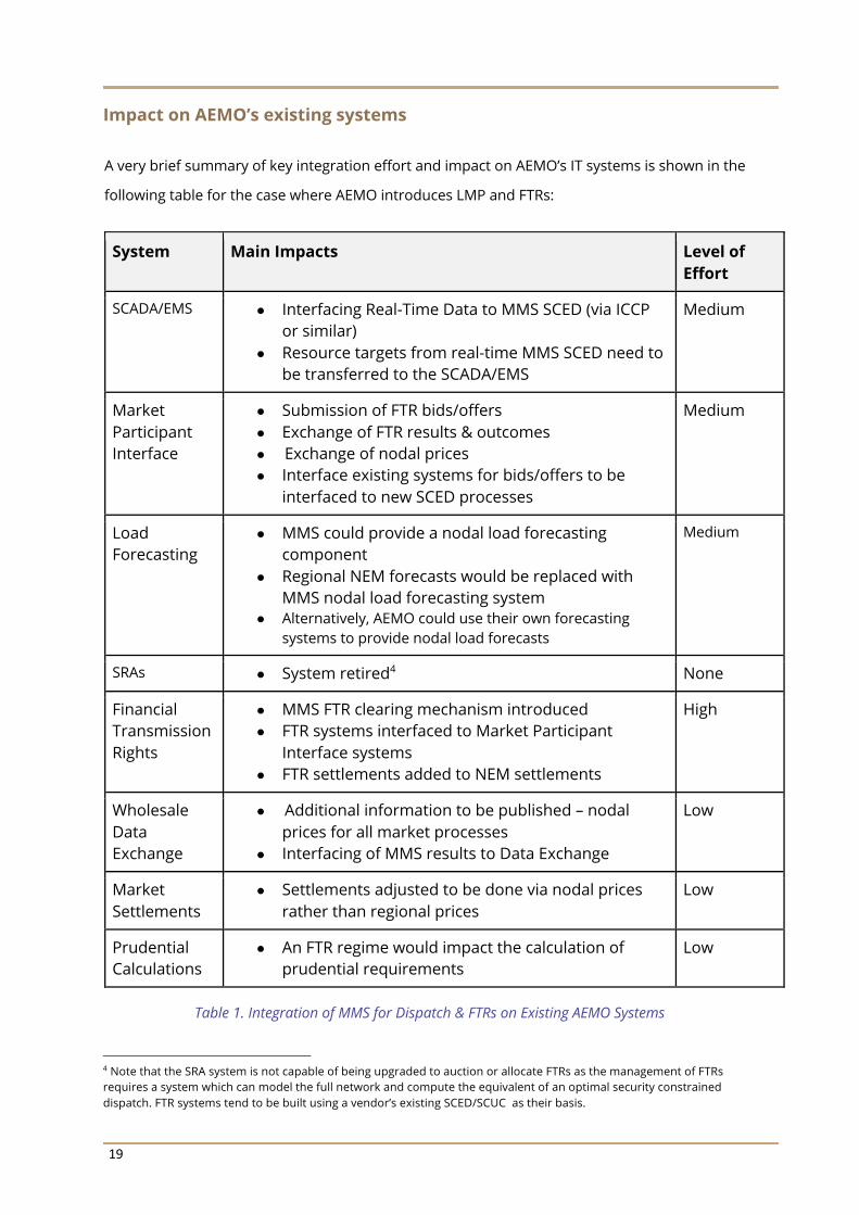
Impact on AEMO’s existing systems

A very brief summary of key integration effort and impact on AEMO’s IT systems is shown in the

following table for the case where AEMO introduces LMP and FTRs:

System Main Impacts Level of Effort

SCADA/EMS ● Interfacing Real-Time Data to MMS SCED (via ICCP or similar)

● Resource targets from real-time MMS SCED need to be transferred to the SCADA/EMS

Medium

Market Participant Interface

● Submission of FTR bids/offers ● Exchange of FTR results & outcomes ● Exchange of nodal prices ● Interface existing systems for bids/offers to be

interfaced to new SCED processes

Medium

Load Forecasting

● MMS could provide a nodal load forecasting component

● Regional NEM forecasts would be replaced with MMS nodal load forecasting system

● Alternatively, AEMO could use their own forecasting systems to provide nodal load forecasts

Medium

SRAs ● System retired4 None

Financial Transmission Rights

● MMS FTR clearing mechanism introduced ● FTR systems interfaced to Market Participant

Interface systems ● FTR settlements added to NEM settlements

High

Wholesale Data Exchange

● Additional information to be published – nodal prices for all market processes

● Interfacing of MMS results to Data Exchange

Low

Market Settlements

● Settlements adjusted to be done via nodal prices rather than regional prices

Low

Prudential Calculations

● An FTR regime would impact the calculation of prudential requirements

Low

Table 1. Integration of MMS for Dispatch & FTRs on Existing AEMO Systems

4 Note that the SRA system is not capable of being upgraded to auction or allocate FTRs as the management of FTRs requires a system which can model the full network and compute the equivalent of an optimal security constrained dispatch. FTR systems tend to be built using a vendor’s existing SCED/SCUC as their basis.

20

MMS cost estimate

Context

Not all of the MMS components listed earlier (in this section) would need to be developed in the

situation that AEMO was to purchase an MMS to implement LMP and introduce an FTR regime.

This section provides a ballpark range of the costs of having an MMS vendor implement the

following aspects of an MMS:

● Market Participation Registration Management System,

● Market Participant Interface (MPI),

● Nodal Load Forecasting System,

● security Constrained Economic Dispatch (SCED) Model including power flow analysis

tools to automatically generate thermal and voltage constraints,

● customisation of SCED to implement a Real-Time Dispatch (RTD) – i.e. 5-minute ahead

NEMDE, Hour-Ahead Projections (HAP) – i.e. 5-minute / hour-ahead Pre-Dispatch, Day-

Ahead Projections (DAP) – i.e. up to 30-minute / 48 hours ahead pre-dispatch and

sensitivities,

● automatic compliance monitoring system,

● FTR auction clearing mechanism,

● FTR settlements system,

● user Interfaces for Market Participants,

● user Interfaces for the Market Operator,

● interfaces to other processes:

○ Market network model management tools/systems

○ Outage management tools/systems

○ SCADA/EMS

○ Results publication ,systems/databases

● offline study systems,

● production and pre-production systems, and

● backup MMS

The range of MMS features is larger than would necessarily need to be implemented, however,

the list provides a reasonable basis for the economic cost-benefit analysis that is presented later.

Also, the number of licences and the extent of the hardware that would be required at AEMO is

21

uncertain. Further, the EMS vendor costs also give indications of what should be reasonable

AEMO costs, should AEMO decide to develop in house components of the MMS.

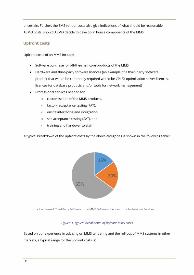
Upfront costs

Upfront costs of an MMS include:

● Software purchase for off-the-shelf core products of the MMS

● Hardware and third-party software licences (an example of a third-party software

product that would be commonly required would be CPLEX optimisation solver licences,

licences for database products and/or tools for network management)

● Professional services needed for:

○ customisation of the MMS products,

○ factory acceptance testing (FAT),

○ onsite interfacing and integration,

○ site acceptance testing (SAT), and

○ training and handover to staff.

A typical breakdown of the upfront costs by the above categories is shown in the following table:

Figure 3. Typical breakdown of upfront MMS costs

Based on our experience in advising on MMS tendering and the roll-out of MMS systems in other

markets, a typical range for the upfront costs is:

22

● 12 million USD to 18 million USD, or

● 17 million AUD to 26 million AUD5

Support & maintenance costs

The support and maintenance costs – paid annually – usually range from 10% to 20% of the

upfront costs discussed in the previous section6. A typical range for the ongoing annual support

and maintenance follows:

● 1.2 million USD to 3.6 million USD, or

● 1.7 million AUD to 5.0 million AUD.

Summary of MMS cost assumptions

A summary of the range of ballpark MMS costing assumptions that we use in this study is shown

in the next table.

The following points should be noted:

• AEMO would likely not need to purchase an entirely new MMS to implement locational

marginal pricing. Only the following components would be required:

o SCED – comprising the Market Dispatch Optimisation Model and Power System

Analysis tools (to generate security limits automatically),

o FTR auction clearing system and FTR settlement system,

o supporting Market Operations database, and

o interfaces to existing IT systems

• if the MMS vendors were put into a competition to provide an MMS, the costs might be

lower than those stated.

Thus, the cost estimates provided in this section are at the upper end of the range of what costs

could occur in practice.

5 Using an exchange rate of 0.71 AUD per 1.00 USD 6 10%-20% of the upfront cost is very typical of an IT support & maintenance fee structure for software systems similar in nature to the MMS

23

Aspect Unit Low Case High Case

Upfront Costs

Hardware & 3rd Party Software AUD million 2.5 3.8

MMS Software Licences AUD million 3.4 5.0

Professional Services AUD million 11.0 16.5

Total AUD million 16.9 25.3

Annual Support & Maintenance Costs

Support & Maintenance AUD million / Year 1.7 5.0

Table 2. MMS costing summary

24

NEM dispatch and pricing

Size of NEM power system

The NEM power system stretches from Port Douglas in Queensland to Port Lincoln in South

Australia and across the Bass Strait to Tasmania – a distance of around 5,000km. There are

approximately 40,000 km of transmission lines.

The transmission network has around:

● 3,200 buses,

● 2,300 transmission lines,

● 1,800 transformers,

● 1,200 substations,

● 550 generating units, and

● 2,000 loads modelled across 800 substations.

The NEM Security Constrained Economic Dispatch

Dispatch and spot pricing are managed in the NEM via the NEM Dispatch Engine (NEMDE).

Cegelec ESCA developed the original dispatch engine in 1998. ESCA was subsequently bought by

ALSTOM and is now part of GE. NEMDE has not undergone any significant functional changes

since the introduction of the FCAS spot market in September 2001. The optimisation of local

FCAS requirements was removed from NEMDE, and generic constraints were used by AEMO to

replace this capability. The transfer of key functions from the NEMDE to generic constraints has

been an ongoing trend with NEM’s security-constrained economic dispatch. Most changes to the

dispatch optimisation process have been done via generic constraints rather than through

explicit modifications to the formulation of the NEMDE optimisation. This trend has been driven

to some extent because the NER requires changes to the NEM optimisation to be independently

audited but has not required generic constraints nor the entire dispatch process to be

independently audited.

25

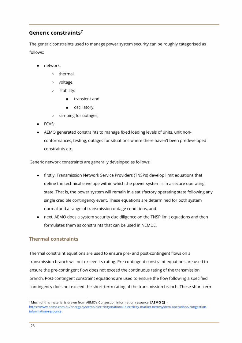
Generic constraints7

The generic constraints used to manage power system security can be roughly categorised as

follows:

● network:

○ thermal,

○ voltage,

○ stability:

■ transient and

■ oscillatory;

○ ramping for outages;

● FCAS;

● AEMO generated constraints to manage fixed loading levels of units, unit non-

conformances, testing, outages for situations where there haven’t been predeveloped

constraints etc.

Generic network constraints are generally developed as follows:

● firstly, Transmission Network Service Providers (TNSPs) develop limit equations that

define the technical envelope within which the power system is in a secure operating

state. That is, the power system will remain in a satisfactory operating state following any

single credible contingency event. These equations are determined for both system

normal and a range of transmission outage conditions, and

● next, AEMO does a system security due diligence on the TNSP limit equations and then

formulates them as constraints that can be used in NEMDE.

Thermal constraints

Thermal constraint equations are used to ensure pre- and post-contingent flows on a

transmission branch will not exceed its rating. Pre-contingent constraint equations are used to

ensure the pre-contingent flow does not exceed the continuous rating of the transmission

branch. Post-contingent constraint equations are used to ensure the flow following a specified

contingency does not exceed the short-term rating of the transmission branch. These short-term

7 Much of this material is drawn from AEMO’s Congestion information resource [AEMO 2] - https://www.aemo.com.au/energy-systems/electricity/national-electricity-market-nem/system-operations/congestion-information-resource

26

ratings allow for some time to elapse before the flow must be reduced to below the continuous

rating of the critical element.

Thermal constraints can be determined directly as a function of generation injections, load off

takes and HVDC flows based on the calculation of shift factors or power transfer distribution

factors for generation and loads and line outage distribution factors for transmission branch

contingencies. The shift factors are dependent on what bus(es) is(are) deemed to be the swing

bus (the balancing bus(es)).

These constraints are based on a specific network state such as system normal, outage of line 60

etc.

Sometimes thermal constraints may be created from a regression analysis using a number of

power system scenarios.

Many thermal constraints are formulated as feedback constraints where the actual power flows

of a network branch are used to adjust the constraint and make it more accurate in real time.

Voltage constraints

Voltage constraints are used for managing transmission voltages so that they remain at

acceptable levels before and after a credible contingency.

Transient stability constraints

Transient stability constraints are used for managing network flows to ensure the continued

synchronism of all generators on the power system following a credible contingency. The

transient stability limit is defined as the maximum power that can be transferred between large

groups of generators while maintaining synchronism following a two-phase-to-ground fault at

the critical location.

Oscillatory stability constraints

Oscillatory stability constraints are used for managing network flows to ensure the damping of

power system oscillations is adequate following a credible contingency. The oscillatory limit

defines the maximum power that can be transferred from one region to another such that any

oscillations resulting from small perturbations on the power system are adequately damped.

27

Limit equations and constraints for voltage, transient and oscillatory

stability

Voltage, transient and oscillatory stability limit equations are generally derived from a large

number of power system studies to ensure an adequate level of accuracy of the limit equation

for a wide range of operating conditions. The power system studies cover variations in the main

variables likely to affect the limit such as a combination of the number of generators online at

each power station, changes in reactive plant on-line, different transfer levels between regions,

and a range of regional demand levels.

A limit equation is then developed by fitting a multi-variable equation to these critical cases (a

multiple regression). The fit of the equation is determined such that it will cover most or all of

the critical cases studied. The limit equation is then linearised into one or more constraints.

A combinatorially large number of potential network constraints

Strictly speaking, each generic network constraint is only valid for a specific network state:

system normal, line 60 outage etc. In practice line outages in northern QLD are unlikely to

change the thermal constraints for SA materially. AEMO classifies groups of constraints

equations that manage particular conditions or situations into constraint sets. For a given

network state, such as system normal or an outage, one or more constraint sets may be

required.

In practice, it is not possible to have the predetermined constraint sets for every possible

network state. For example, to cater for every potential network state corresponding to a single

transmission line outage would require 2,300 groups of constraints and each of these groups of

constraints would have to be able to manage forced outages on all other transmission lines,

generating units and loads. Furthermore, if you catered for system states involving more than

one line outage, the number of predetermined constraints could run into the millions. Clearly,

the approach of trying to predetermine all constraints to be used by NEMDE to guarantee an

optimal security-constrained dispatch is a combinatorially infeasible problem, so in practice,

system normal and only the most critical potential contingency events and planned outages can

be the subject of focus. As a consequence, the dispatches may not always be optimal.

28

Constraint margins

Safety margins are added to the TNSPs limit equations to ensure that the boundaries in all of the

critical cases are covered by the limit equation. Similarly, AEMO will add margins to the

constraint equations to account for operational issues. Between the TNSPs and AEMO, margins

will be added for:

● statistical errors (the statistical margins include the use of the 95 and 99 percent

confidence intervals);

● modelling approximations (assumptions about system conditions, approximations of

generator control systems etc.);

● dispatch errors;

● non-conformance of generators;

● measurement errors.

Measurement errors can affect many terms used in constraint equations including

interconnector flows and generator outputs. Measurement variances can result in errors when

determining the left and/or right-hand side values of the constraint equation.

Constraint orientation

Because the regional reference prices are determined from the shadow price of the regional

energy balance equation, the regional reference node’s load cannot appear in any generic

constraint if the correct energy marginal price is to be determined. Thus, many generic

constraints, particularly thermal constraints, have to be reformulated in a way that is often

counter-intuitive. This process of formulating constraints, so that the correct energy marginal

price for the regional reference node can be determined directly from the regional energy

balance equation, is referred to as constraint orientation.

29

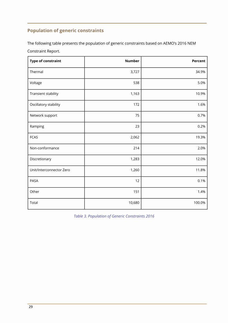
Population of generic constraints

The following table presents the population of generic constraints based on AEMO’s 2016 NEM

Constraint Report.

Type of constraint Number Percent

Thermal 3,727 34.9%

Voltage 538 5.0%

Transient stability 1,163 10.9%

Oscillatory stability 172 1.6%

Network support 75 0.7%

Ramping 23 0.2%

FCAS 2,062 19.3%

Non-conformance 214 2.0%

Discretionary 1,283 12.0%

Unit/Interconnector Zero 1,260 11.8%

PASA 12 0.1%

Other 151 1.4%

Total 10,680 100.0%

Table 3. Population of Generic Constraints 2016

30

Figure 4. Proportion of the type of NEM generic constraints 2016

Since the 2016 report, AEMO has developed some new constraint classes: ROC frequency (rate of

change of frequency) and system strength. Also, there are constraints to manage negative SRA

revenues.

Modelling losses in the NEM

The NEM market model is a substantially simplified model of the transmission network,

particularly in the area of modelling transmission losses. These simplifications mean that

transmission network characteristics and limits are in many cases approximated (usually with a

conservative bias). Thus, the actual NEM dispatch may be sub-optimal when compared to an

optimisation which more accurately models the losses. This is not a reflection of AEMO’s

implementation of the dispatch optimisation but rather is a reflection of the degree to which the

National Electricity Rules simplify modelling the actual physical network in general and the

modelling of losses in particular.

The NEM dispatch model is an approximate form of locational marginal pricing model in that the

transmission constraints are modelled, and transmission losses are approximately modelled. In

31

a full nodal model, the losses for all power transfers would be dynamically modelled, effectively

giving rise to dynamic transmission loss factors during every dispatch interval. In the case of the

NEM, static marginal loss factors are used for flows within each region and inter-regional loss

equations are used for flows between regions. Further, the static MLFs are not even used to

model losses; they are only used as price multipliers of the bids and offers in NEMDE. All intra-

regional losses are incorporated into the NEM dispatch via the regional load forecasts which

include both the regional loads and the intra-regional transmission losses.

Generators, loads and intra-regional losses

Intra-regional losses are electrical energy losses that occur due to the transfer of electricity

between a regional reference node and transmission network connection points in the same

region.

The NEM uses intra-regional loss factors, generally called MLFs, to model intra-regional transfers.

These MLFs are estimates of the marginal electrical energy required for electricity to be

transmitted between a regional reference node and a transmission network connection point in

the same region.

The regional reference node is in effect the reference point for intra-regional loss calculations

with a loss factor by definition of unity (electricity generated or consumed at the regional

reference node has no losses when referred to the regional reference node).

Connection points that generally export electricity to the regional reference node, would be

expected to have loss factors less than one reflecting losses consumed in transmitting to the

reference node (one MWh injected at an exporting connection point provides a MWh less the

losses at the regional reference node).

Connection points that generally import electricity from the regional reference node would be

expected to have loss factors greater than one reflecting losses consumed in transmitting from

the regional reference node (one MWh withdrawn at an importing connection point requires a

MWh plus the losses to be injected at the regional reference node).

If the flow is always in one direction, there will generally be just one MLF calculated for a

connection point. Where the flows at a connection point may flow in either direction (tidal flows)

or there are other circumstances which make the approximation of a single MLF too inaccurate,

32

two MLFs may be calculated and used by AEMO. MLFs are updated annually – the same MLF(s)

apply for a whole year.

Calculation of Marginal Loss Factors (MLF)

MLFs are calculated on a forward-looking basis, for the year ahead, using a full network model of

the NEM based on a system snapshot8. AEMO uses the TPRICE software package to calculate the

loss factors. TPRICE solves the power flow problem for each half-hour based on projected half-

hourly load and generator data. For each half-hour, TPRICE essentially calculates nodal prices

ignoring network constraints.

For each half hour, a connection points half-hourly MLF is just the ratio of its nodal price to the

regional reference node’s nodal price. For connection points with just one fixed MLF, its value is

just the weighted average over the modelled year of the half-hourly MLFs. Generation loss

factors are weighted by generator output and load loss factors by load consumption. These

MLFs are simply weighted averages (single point approximations) to these MLF distributions.

Marginal loss factors can vary considerably from one half hour to another over a year, see

example in Figure 5.

Figure 5. Example of the distribution of half-hourly MLFs

8 The system snapshot network model used by AEMO reflects all normally connected equipment and any network augmentations due to be in operation in the following year.

33

Use of MLFs

It is an important distinction that while MLFs are calculated based on expected losses referenced

to the regional reference node, the MLFs are not used to explicitly model intra-regional losses in

the NEM dispatch process. Instead, they are used as:

● price multipliers that can be applied to the regional reference price to determine the

local spot price at each transmission network connection point and virtual transmission

node, and

● price adjustments to generator offer prices and to load bid prices to reflect a generator’s

effective offer price or a load’s effective bid price when referred to the regional reference

node to which that connection point is assigned.

Inter-connector losses

Inter-regional losses are electrical energy losses due to a notional transfer of electricity through

regulated interconnectors from the regional reference node in one region to the regional

reference node in an adjacent region.

AEMO is required to determine inter-regional loss factor equations. This is done by developing

an inter-regional loss equation that calculates the average or expected losses as a function of the

power flows on an interconnector. The loss equation is generally a quadratic function of power

flows. These equations are updated annually.

In NEMDE, piecewise linear approximations of the inter-regional loss equations are used, and the

dispatch optimisation automatically trades off the incremental costs of greater interconnector

flows versus greater use of intra-regional generation.

Inter-regional loss equations are not dynamically calculated (i.e. based on the actual

configuration of the transmission network at each point in time) but are based on linear

regression equations which fit a model to inter-regional losses in terms of interconnector flows

and any other explanatory variables that AEMO regards as necessary, such as regional demands.

Since these equations are to be used in the NEMDE linear programming optimisation, generator

terms, which are to be optimised, cannot be included as explanatory variables.

34

Summary of loss models

The key points to note about the loss models used in the NEM are as follows:

● the losses associated with intra-regional generators are indirectly modelled by MLFs,

which are used as price multipliers. Within the dispatch process, when dispatching

generators to meet the regional demand, generator outputs are treated as lossless,

● regulated interconnectors use predefined quadratic loss functions to estimate the losses

for power transfers from the regional reference node in the sending region to the

regional reference node in the receiving region. For regulated interconnectors, losses

are explicitly modelled in the dispatch process based on the precalculated loss functions.

The loss functions may not always be accurate if there is a set of outages which affect the

interconnector, and

● Scheduled Network Service Providers (SNSPs), DC interconnectors, use a hybrid model

for losses which is a combination of linear loss models based on the MLFs of the

connecting terminals for within region flows and a quadratic loss model for flows over

the physical SNSP. For SNSPs, the losses are explicitly modelled in the dispatch process.

Regional and locational pricing in the NEM

Even though NEMDE does not directly produce LMPs, a form of generator LMPs can be inferred

from NEMDE’s output. These are generator LMPs based on the regional reference price, the

generator’s MLF and the constraint costs associated with its generation.

For each generic constraint associated with managing power flows over the transmission system

in a dispatch interval, NEMDE will produce a shadow price for the constraint. The shadow price

represents the marginal costs of the constraint. If the right-hand side of the constraint were

increased by one unit, the shadow price indicates how much the system-wide costs would be

changed. If the constraint is not binding, then it will have a shadow price of zero.

For each constraint, the increase in the system-wide cost of increasing a generating unit’s output

is the negative of the shadow price of the constraint times the generator’s coefficient on the left-

hand side of the constraint. Thus, the total constraint cost of increasing a generator’s output is

minus the sum of each constraint’s shadow price times the generator’s left-hand side constraint

coefficient.

35

A LMP for a generator would be as follows:

LMP = regional reference price x MLF – sum of generator’s constraint costs

= regional reference price x MLF + sum of generator’s constraint coefficient x

shadow price of constraint for each constraint

36

Locational Marginal Pricing options

Introduction

The AEMC requested that we address the costs of introducing LMP and FTRs to varying degrees

of effectiveness. In particular, the AEMC requested that we look at the following costs:

● the costs to the market operator and participants of introducing LMP and FTRs, while

maintaining the existing regional reference price and loss framework, that is largely using

the existing NEMDE framework and producing nodal generator prices based on

constraint costs and continue with a single regional reference price (the base case),


with a volume-weighted average price, that is developing nodal prices for all generation

and load nodes but with non-dynamic loss factors and the calculation of a load weighted

regional reference price, and

● incremental costs (relative to the base case) of introducing a full network model,

dynamic losses and nodal prices for loads and generation and the calculation of load

weighted regional prices.

For the AEMO systems, based on our experience, we expect that the most efficient way to

introduce LMP with dynamic marginal losses and FTRs is to purchase standard off the shelf

market management software (MMS) from one of the main energy management system (EMS)

vendors such as GE, ABB and Siemens. If this is done, then the calculation of volume-weighted

average prices (VWAPs) for regions or zones would be trivial.

For the option of LMP and FTRs without dynamic losses, the most effective way of delivering this

was not clear. Would it be better to adapt NEMDE and change all of the thousands of generic

constraints so that each nodal load had the correct coefficients in each constraint in order to

produce nodal prices or would be better to purchase off the shelf market management

software? If off the shelf software were purchased there would be no sensible reason to

downgrade it to using just fixed marginal loss factors as this would lead to less efficient

dispatches and perhaps a reduction in system security for no cost-benefit. Thus, in this report,

we only explore the option of using the NEMDE framework to produce generation and load LMPs

with fixed MLFs.

37

Additional benefits from SCED with full nodal pricing

The use of LMPs with dynamic losses is likely to lead to more efficient investments in

transmission and generation, as well as more efficient market participant behaviour and more

economic dispatches. These benefits are being investigated by the AEMC. In addition to these

benefits of nodal pricing, a new SCED optimisation, that dynamically generates thermal and

voltage constraints and dynamic marginal losses, is likely to lead to materially more efficient

dispatches because many of the NEM’s generic constraints that are used to manage power flows

have safety margins which are built into them to manage the risks of:

● statistical errors,

● modelling approximations (assumptions about system conditions, approximations of

generator control systems, etc.),

● dispatch errors,

● non-conformance of generators, and

● measurement errors.

If the constraints are developed on the fly, then the actual network outages, generator outages,

nodal loads, non-conformance of generators, power flows etc. are known. Thus, dynamically

generated voltage and thermal constraints should effectively reduce these margins when it is

safe to do so or on some occasions if there are security issues tighten up these constraints.

Furthermore, with dynamically generated constraints, only the relevant voltage and thermal

constraints will be used in the security-constrained dispatch. No thermal or voltage constraints

that were designed for another network configuration will be left in the optimisation to over

constrain the dispatch and increase dispatch costs.

Another advantage of purchasing a new SCED is that all of the FCAS constraints could be

properly formulated as part of the optimisation and thus be able to more efficiently manage

FCAS local and zonal requirements and better manage the co-optimisation of network flows,

FCAS global and local requirements and the actual dispatch of generating units. Further, a clear

mathematical optimisation approach would make it easier to introduce changes to the FCAS spot

market such as a very fast contingency service, inertia services, locational regulation services and

so on.

38

Lastly, with dynamically generated thermal and voltage constraints, the dispatch process will be

better able to securely manage unexpected network states resulting from major weather events

such as bushfires and cyclones.

Existing AEMO systems and sources of AEMO costs

Figure 6. Diagram of systems related to NEM dispatch and pricing

The relationship between the AEMO systems outlined in the figure above and the general MMS

components outlined in figure 2 are presented below.

AEMO Systems Standard MMS

Plant registration data Market registration system

SCADA SCADA/EMS

Average MLFs Power system tools

Network data including line ratings and plant outages

Market operations database and outage management system

Load forecasting Nodal load forecasting

VRE generation forecasting Not standard

NEM Dispatch EngineDispatch and pre-

dispatch

Load forecasting

Solar generation forecasting

Wind generation forecasting

AGC system

SCADA system

Causer pays

Determination of MLFs

Bids and offers

Participant use interface

Meter data management

Constraints

MSATS

Weather forecasts

Wholesale data exchange

Registration data

Settlements

Network model, line ratings and

plant outages

39

AEMO Systems Standard MMS

Generic constraints Power system tools + stability constraints

Bids and offers Market participant interface

Security constrained dispatch (NEMDE + generic constraints)

SCED (market dispatch optimisation + power system tools)

Pre-dispatch and price sensitivities SCED (market dispatch optimisation + power system tools)

AGC SCADA/EMS including AGC

Meter data management Metering

Spot market settlements Settlements system

Causer pays for regulation Settlements system

Wholesale data exchange Market database

Participant interface (Spot Market) Market participant systems

Prudential management system Prudential requirements

Settlement residue auction N/A replaced by FTR system

Plant registration data Market registration system

The following table provides our preliminary overview of what AEMO systems are likely to

require changes in order to implement each of the three LMP options, based on our experience.


System / activity Locational pricing for generators using current NEMDE

Locational pricing for generators and loads using current NEMDE

Locational pricing with new security-constrained dispatch system

Plant registration data

No change No change No change

SCADA No change No change No change

Average MLFs No change No change Not required, dynamic loss factors calculated by SCED

Network data including line ratings and plant outages


Load forecasting No change Nodal load forecasts required

Nodal load forecasts required

40


VRE generation forecasting


Generic constraints No change All generic constraints have to be updated to include nodal load coefficients on RHS

Thermal and voltage constraints can be automatically generated. Stability constraints would have to be updated. Many FCAS generic constraints could be directly formulated in the optimisation. A substantial portion of the generic constraints would no longer be required.

Bids and offers No change No change No change

Security constrained economic dispatch (SCED)

Minimal change Minimal change New SCED system

Pre-dispatch and price sensitivities

Must provide nodal price forecasts for generators and dispatchable or controllable loads



AGC No change No change No change

Meter data management


Spot market settlements

Minimal change Minimal change Minimal change

Causer pays for regulation


Wholesale data exchange

Increased information to be provided for pre-dispatch and increased spot price information following dispatch



Participant interface Minimal change other than for FTRs

Minimal change other than for FTRs


41


Prudential management system

Modest enhancements to deal with nodal prices versus regional prices



Settlement residue auction

No longer required No longer required No longer required

FTR Auction and Allocation Optimisation

Significant enhancements to the NEMDE/PD systems to facilitate an intertemporal optimisation

Significant enhancements to the NEMDE/PD systems to facilitate an intertemporal optimisation

Based on the new SCED/FTR system from MMS vendor

FTR management New system New system New system, part of SCED/FTR package from MMS vendor

FTR settlement New system New system New system, part of SCED/FTR package from MMS vendor

Table 4. AEMO systems that may require changes to implement nodal pricing

Shared costs with other new systems

We understand AEMO is investigating replacing and upgrading other systems that could share

the same infrastructure as an off the shelf nodal pricing SCED system. In particular, AEMO is

looking at replacing the existing ST PASA system with a system that better models the physical

power system and can automatically generate network security constraints for unusual

situations. This system is likely to be based on an off the shelf SCED/SCUC (Security Constrained

Unit Commitment) system which would require nodal load forecasts. Also, AEMO is looking at

the possibility of creating a forward market such as a one or two day ahead market. This is likely

to require new SCED/SCUC like software. Finally, if there is a revision of FCAS to better integrate

with increased VRE and batteries, then there is likely to be a need to upgrade NEMDE or replace

it with a new SCED.

42

AEMO costs for the various options

Because of the very short time available to us to conduct this study, we were unable to get

estimates from AEMO of what the effort and costs would be for AEMO to implement various

system components of the different options. So, what we have done is used the MMS vendors

costs as indicative costs of what the efficient cost would be for AEMO to implement each

component. Following this logic, in this section, we first estimate the costs for Option 3, then

Option 1 and then Option 2.

AEMO costs for Option 3

Option 3 involves introducing a new SCED to implement LMP, establishing a nodal load

forecasting system and introducing FTRs – both the clearing mechanism and a settlement

system. As described in section 3, the upfront costs (see Table 3) of an MMS that provides the

essential components for this ranges from about 16.9 to 25.3 million AUD, with annual support

and maintenance costs ranging from 1.7 (10%) million AUD/year to 5.0 million AUD/year. The

actual costs would vary depending on the size of the power system and how many licences

required: say 2 x real-time operations, 2 x hot standby/backup, 2 x for training, 2 for offline

studies and so on. Also putting the MMS vendors into a competition to provide systems may

yield lower costs.

For the purpose of the foregoing estimates, we take the higher end of the range provided earlier

and apply some judgment to the composition of the total costs of the MMS from Table 3. This is

then broken down to individual costs for the following components:

● Nodal Load Forecasting system,

● SCED system:

○ Real-Time 5-minute nodal dispatch and pricing,

○ 5-minute Pre-Dispatch,

○ 30-minute Pre-Dispatch and sensitivities,

○ integration and interfacing to other systems/components,

○ user interfaces,

○ FAT, SAT and training,

○ hardware,

○ production and pre-production hardware and software,

○ offline study machines, and

43

○ backup systems

● FTR system

○ FTR Auction and Allocation optimisation,

○ FTR participant interface,

○ FTR management,

○ FTR settlement,

○ integration and interfacing to other systems/components,

○ user interfaces,

○ FAT, SAT and training,

○ hardware,

○ production and pre-production hardware and software,

○ offline study machines, and

○ backup systems

Estimates for the upfront and annual costs for Option 3 are provided in Table 5. It is argued that

these costs could be used as proxy costs for the internal costs of AEMO – since they are linked to

MMS costs, then it could be expected that AEMO’s costs would be similar (otherwise, outsourcing

to an MMS vendor would be done).

System / activity Locational pricing for generators using current NEMDE

Upfront Cost (AUD)

Ongoing Cost (AUD/year)

Plant registration data No change 0 0

SCADA No change 0 0

Average MLFs Not required, dynamic loss factors calculated by SCED 0 -200,000

Transmission line ratings and network data No change 0 0

Load forecasting Nodal load forecasts required 2,040,845 408,169

VRE generation forecasting No change 0 0

Generic constraints Thermal and voltage constraints can be automatically generated. Stability constraints would have to be updated. Many 2,820,000 705,000

44

FCAS generic constraints could be directly formulated in the optimisation. A substantial portion of the generic constraints are not required.

Bids and offers No change 0 0

Security constrained economic dispatch (SCED) New SCED system

10,901,408 2,180,282


Must provide nodal price forecasts for generators and dispatchable or loads

AGC No change 0 0

Meter data management No change 0 0

Spot market settlements Minimal change 500,000 100,000

Causer pays for regulation No change 0 0

Wholesale data exchange Increased information to be provided for pre-dispatch and increased spot price information following dispatch 1,000,000 200,000

Participant interface (Spot Market)

Minimal change other than for FTRs 300,000 60,000


Modest enhancements to deal with nodal prices versus regional prices 300,000 60,000

Settlement residue auction No longer required 0 -200,000

FTR auction and allocation optimisation


5,678,873 1,135,775

FTR participant interface New system, part of SCED/FTR package from MMS vendor

FTR management New system, part of SCED/FTR package from MMS vendor

FTR settlement New system, part of SCED/FTR package from MMS vendor

Totals 23,541,127 4,449,225

Table 5. Investment and ongoing costs for Option 3

45


For Option 1, we looked at the costs for AEMO to introduce LMP for generators and charging

customers using a single regional reference price. This would be done via determining a nodal

price for each dispatchable unit based on the regional reference price; it’s MLF and the

constraint costs associated with the unit. NEMDE produces all of the data required for this

scenario. Thus, the main changes required for this option would be:

● the calculation of generating unit LMPs in NEMDE or the settlements system, it is

probably easier to do it in NEMDE’s post-processing of the optimisation’s results,

● some enhancements to the pre-dispatch information to provide generators projections

of their LMPs as well as regional reference price projections and sensitivities,

● spot market settlements would require minimal changes, as all that is required is the

settlements would now need to refer to the generator’s own locational price,

● the wholesale data exchange and participant interface would have to be updated to cater

for the extra LMP data, and

● there would have to be significant enhancements to cater for the FTR auctions,

allocations and settlements.

Before we address the AEMO costs with this option, we will address some of the financial issues

with this option. If full LMP is introduced, then the revenue gained from customers is always

greater than the amounts paid out to customers. This still applies if all customers are charged

the load weighted average price. However, if all customers are charged the regional reference

node price (the LMP at the regional reference node), there is no guarantee that the revenues

from customers will always be able to pay the generator costs. This could occur if there were

really high LMPs occurring in a number of load nodes but not at the regional reference node.

Also, the same problem can manifest itself if most FTRs are referenced to the regional reference

node. That is there could be a shortfall of revenue to pay out the FTRs. Similarly, if the FTR

allocation is based on a physically feasible security-constrained dispatch (the simultaneous

feasibility requirement for FTRs), then there could be a substantial shortfall of FTRs required to

hedge the loads of customers.

As a consequence of the two points above, Option 1 has some substantial financial and risk

management deficiencies.

The preliminary indicative costs for Option 1 are presented in Table 6.

46

System / activity Nodal pricing for generators using current NEMDE

Upfront Cost (AUD)



SCADA No change 0 0

Average MLFs No change 0 0

Transmission line ratings and network data

No change 0 0

Load forecasting No change 0 0


No change 0 0

Generic constraints No change 0 1,346,700



Minimal change 200,000 0



200,000 0

AGC No change 0 0



Causer pays for regulation No change 0 0

Wholesale data exchange Increased information to be provided for pre-dispatch and increased spot price information following dispatch

1,000,000 200,000



300,000 60,000



300,000 60,000


No longer required 0 -200,000

FTR auction and allocation optimisation

Significant enhancements to the NEMDE/PD systems to

5,678,873 1,135,775

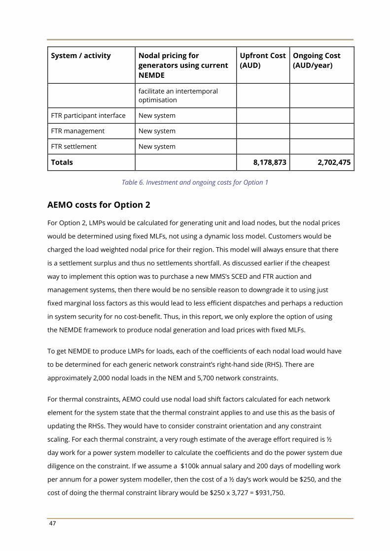
47

System / activity Nodal pricing for generators using current NEMDE

Upfront Cost (AUD)


facilitate an intertemporal optimisation

FTR participant interface New system

FTR management New system

FTR settlement New system

Totals 8,178,873 2,702,475



For Option 2, LMPs would be calculated for generating unit and load nodes, but the nodal prices

would be determined using fixed MLFs, not using a dynamic loss model. Customers would be

charged the load weighted nodal price for their region. This model will always ensure that there

is a settlement surplus and thus no settlements shortfall. As discussed earlier if the cheapest

way to implement this option was to purchase a new MMS’s SCED and FTR auction and

management systems, then there would be no sensible reason to downgrade it to using just

fixed marginal loss factors as this would lead to less efficient dispatches and perhaps a reduction

in system security for no cost-benefit. Thus, in this report, we only explore the option of using

the NEMDE framework to produce nodal generation and load prices with fixed MLFs.

To get NEMDE to produce LMPs for loads, each of the coefficients of each nodal load would have

to be determined for each generic network constraint’s right-hand side (RHS). There are

approximately 2,000 nodal loads in the NEM and 5,700 network constraints.

For thermal constraints, AEMO could use nodal load shift factors calculated for each network

element for the system state that the thermal constraint applies to and use this as the basis of

updating the RHSs. They would have to consider constraint orientation and any constraint

scaling. For each thermal constraint, a very rough estimate of the average effort required is ½

day work for a power system modeller to calculate the coefficients and do the power system due

diligence on the constraint. If we assume a $100k annual salary and 200 days of modelling work

per annum for a power system modeller, then the cost of a ½ day’s work would be $250, and the

cost of doing the thermal constraint library would be $250 x 3,727 = $931,750.

48

For the voltage and stability constraints which were based on power system modelling and

regression analysis, the time would be much more. If we assume that the relevant modelling

documentation was available, then a very rough estimate of the average effort required is four

days of work for determining the coefficients and power system due diligence on the constraint.

This would give a cost of $2,000 per constraint and the following initial costs:

Type of network constraint

Number Cost per constraint

Total Can be automatically generated

Costs for new SCED

Thermal 3,727 250 931,750 Yes 0

Voltage 538 2,000 1,076,000 Yes 0

Transient stability

1,163 2,000 2,326,000 No 2,326,000

Oscillatory stability

172 2,000 344,000 No 344,000

Network support

75 2,000 150,000 No 150,000

Total 5,675 8,250 4,827,750 2,820,000

Table 7. Estimated cost for the calculation of constraint coefficients

In addition to the initial costs of updating the constraints for options 2 and 3, there are ongoing

costs associated with maintaining a library of generic network constraints. If we assume that

1/10 of constraints need a major update per annum requiring two man-days per thermal

constraint and 10 for other network constraints, then we get the rough estimates of annual costs

below.


Number Number updated or reviewed annually

Cost per constraint


Costs for new SCED

Thermal 3,727 373 1000 372,700 Yes 0

Voltage 538 54 5,000 269,000 Yes 0

Transient stability

1,163 116 5,000 581,500 No 581,500

49



Cost per constraint


Costs for new SCED

Oscillatory stability

172 17 5,000 86,000 No 86,000

Network support

75 8 5,000 37,500 No 37,500

Total 5,675 568 1,346,700 705,000



Cost per constraint

Total Can be automatically

generated

Costs for new SCED

Table 8. Estimated cost for the maintenance of constraint coefficients

The preliminary indicative costs for option 2 are presented in Table 9.

System / activity Nodal pricing with new security-constrained dispatch system

Upfront Cost (AUD)



SCADA No change 0 0

Average MLFs Not required, dynamic loss factors calculated by SCED

0 0

Transmission line ratings and network data

No change 0 0

Load forecasting Nodal load forecasts required 2,040,845 408,169


No change 0 0

Generic constraints Thermal and voltage constraints can be automatically generated. Stability constraints would have to be updated. Many FCAS generic constraints could be directly formulated in the optimization and many no longer required.

4,827,750 1,346,700

50

System / activity Nodal pricing with new security-constrained dispatch system

Upfront Cost (AUD)




New SCED system 200,000 0



200,000 0

AGC No change 0 0



Causer pays for regulation

No change 0 0

Wholesale data exchange Increased information to be provided for pre-dispatch and increased spot price information

1,000,000 200,000



300,000 60,000



300,000 60,000


No longer required 0 -200,000

FTR Auction and Allocation Optimisation


5,678,873 1,135,775

FTR participant interface New system, part of SCED/FTR package from MMS vendor

FTR management New system, part of SCED/FTR package from MMS vendor

FTR settlement New system, part of SCED/FTR package from MMS vendor

Totals 15,047,468 3,110,644


51

Overall comparison of costs

In order to summarise the overall findings for this section:

● Figure 7 shows a comparison of the upfront costs for each option considered, and

● Figure 8 shows a comparison of the ongoing costs for each option considered.

Figure 7. Comparison of upfront costs for each option

Figure 8. Comparison of ongoing (annual) costs of each option

52

Participant costs

The estimation of costs was based on the Information Technology changes required for each of

the different types of participant categories in the National Electricity Market. The costs reflect

the additional costs that would be associated with the implementation of Locational Marginal

Pricing for the case of generation LMPs and load weighted average prices for load customers and

the case of LMP for both generation and loads have both been considered.

An important assumption that has been used in the estimation of participant IT costs for this

paper is that only additional costs have been considered in this estimation, such as additional

resources employed to implement the changes associated with Location Marginal Pricing or

vendor charges to enhance software, and does not include the costs associated with the

redeployment of internal resources that would have been expended regardless of the

implementation of the proposed market changes.

Recent experience with the participant submissions associated with the implementation of five-

minute settlement in the NEM would suggest that many of the very high IT costs in those

submissions may have included significant costs associated with the upgrading or replacement

of legacy IT systems rather than for the reform itself. Also, the quoted high costs were then used

as part of the justification for not proceeding with the reform at all and then to subsequently

delay the implementation of the five-minute settlement market reform.

The methodology in this report is an attempt to accurately reflect the true incremental costs

associated with the implementation of IT systems for location marginal pricing based on the

authors’ market experience for an initial indication of costs when interviews and investigations of

representative market participants for each of the key categories of participants are outside of

the scope of this present investigation.

Types of participants

The participant costs estimation has been made by segmenting the participants into

representative groups based upon the size and nature of the organisations, estimation of the

number in each category and an initial assessment of the type of IT systems that would be used

by the members of each category and the implications of Locational Marginal Pricing for each of

those identified systems.

53

The numbers estimated for each category have been made at the organisation level rather than

the individual registered NEM participant. For example, an organisation such as Pacific Hydro

would count as one organisation rather than the eight registered generation participants that are

managed by that organisation, as the IT resources would be shared over the individual

generators. Also, it should be noted that organisations will traverse some categories; gentailers

are considered to be vertically integrated companies that have significant generation and retail

portfolios and are considered as a single category, whereas many large generators will also have

a retail arm that is much less significant than the generation activity but has been considered in

the estimation large generators.

Generator participants

The number of entities included in the generator categories has been based on the organisation

entities found in [CER 1]. The large generators category participants were considered to be the

top ten generators based on the annual electricity production included in the “Greenhouse and

energy information for designated generation facilities 2018-19” report published by the Clean

Energy Regulator.

Retail participants

Figure 9. Structure of retail electricity businesses in the NEM

54

The retail participant categories are dominated by the large gentailers that have significant

market share in the Australian NEM and many of the larger retail participants that also have

associated generation organisations (shown as “arms-length” in the figure above) as distinct from

retailers with no associated generation assets [AEMC 1]. For the “arms-length” retailers, the

generation and retail organisations are considered to be distinct and have been separately

counted in the cost estimations whereas the large gentailers are considered as their own distinct

participant category.

It should be noted that the retail organisations are part of a dynamic market as retailers start,

cease trading, and are absorbed into other retailers, so it is more difficult to estimate accurate

numbers of retail organisations than other categories of participants.

Other participants

Participant categories, other than retail and generation participants, that have been considered

to require IT changes associated with the implementation of Locational Marginal Pricing are

Small Generation Aggregators (SGA), non-scheduled load participants and distribution network

service providers. The numbers of these participants are difficult to exactly determine, but the

numbers in this cost estimation are based on documents [AEMO 1], [AER 1] and [AEMC 2].

Cost estimation

For each category of participant, each of the types of IT systems that each participant type for

each required market function would already have been implemented are considered, and then

the cost of enhancements to those systems to support Locational Marginal Pricing has been

estimated.

Spot market costs

The implications of Locational Marginal Pricing for spot trading is relatively insignificant in

comparison to the major changes associated with the upcoming change to five-minute dispatch

and settlement. Small generators and other participants that offer or bid into the NEM would

need to change systems to remove the existing Marginal Loss Factors for the prices of the

availability bands and also in the application of the minimum and maximum prices.

Small participants typically use the AEMO EMMS system for submitting offers or bids into the

market for energy and use some form of commercial bidding system or another system such as

55

an operation or plant control system that incorporates a market offer feature to make their

submissions to AEMO. Larger generators would typically use a purpose-built trading system or

portfolio optimiser that is either developed in-house or from a third-party vendor that specialises

in this type of software.

It would be expected that for most commercial systems or in-house developments, the changes

required for the participant spot market functions would be relatively minor and may even be at

no additional cost to the participant as part of their commercial support arrangements.

Wholesale costs

Most market participants would have relatively low numbers of wholesale contracts to

administer and settle and therefore use generic tools, such as MS Excel to settle those contracts.

Given the assumption of a long lead time before the introduction of Locational Marginal Pricing

into the NEM of at least four years, most existing contracts would not extend over the start of the

proposed market design. Some Power Purchase Agreements do exist that are greater than five

years in duration, and therefore systems would need to be adjusted to match a changed or a

renegotiated reference price such as a regional load weighted average price rather than the

regional reference price that would be the most likely basis of the present contract.

Large retailers or portfolio generators would typically use a commercial contract management

system or a large internally developed system to handle settlement of a potentially wide range of

contract types and forms. Again, most contracts would typically not extend over the start of the

market implementation of Location Marginal Pricing, but the long-term contracts would need to

be renegotiated, and contract settlement terms changed.

The contract systems would need to be enhanced to allow for the specification of the possible

range of locational reference price options for new contracts, as well as handle new contract

types such as Financial Transmission Rights (FTR). The actual form of the FTR contracts would be

a common form of swaps. However, the contract systems may need to be able to associate FTR

and other forms on contracts for reporting and risk management purposes.

Retailer costs

Retail systems would need to be modified for Locational Marginal Pricing for the option of a

complete implementation of the market reform for both generation and loads. Retail systems

would need to be modified to ensure that location prices are used for the aggregated retail loads

56

in their portfolio. For small retailers, it is expected that the enhancements to support LMP would

be implemented in their commercial retail systems and may not require additional expenditure,

as market changes could form part of their existing support contracts.

Large retailers would also use commercial or in-house developed retail systems, and these

would need to be enhanced, but also may need to explicitly handle large customer loads that

require individual adaptation to LMP based contracts.

Market data costs

The implementation of LMP would require a major enhancement and increased data volumes

for the AEMO Market Management System (MMS) RDBMS based market data, although it is not

expected that the present mechanisms for delivery of the market data would need to be

changed or upgraded. It is assumed that small and medium-size generators would not need to

capture a large range of the nodal prices, but as the complexity and range of generation in a

participant’s portfolio increases, so would the requirement to capture a more varied and sizable

range of nodal data.

Many large generators and retailers, especially when mergers, acquisitions and new separately

financed developments occur, may run multiple instances of the MMS database and therefore

their costs would be increased with each separate implementation of the MMS RDBMS.

Small retailers and medium-size retailers would most likely not need to capture a large increase

in data volumes for nodal prices and would be dependent on the number of large loads and

varied locations that they have in their customer portfolio.

Risk management costs

The estimation of the participant costs for the enhancement of risk management systems is the

most challenging cost category as there is a wide range of systems and tools deployed across the

market that is not necessarily related to the size of the organisation or portfolio, but rather the

sophistication of the trading operations, accepted levels of risk aversion and the market

segments in which an organisation generates, such as fast start plant.

Small participants in retail and generation may have no formal risk systems, as their contractual

positions are relatively straightforward and do not warrant greater expenditure on risk

management systems. Many participants in this category would perform their required risk

57

management functions using spreadsheets or based upon reports generated based on AEMO

MMS market data and from other trading or operational software systems.

However, many larger generators and retailers have very sophisticated risk management

systems that are often a combination of vendor systems, including associated systems that

handle other organisational functions such as contract or operations management, and in-house

developed systems ranging from spreadsheets, reporting systems and full risk management

systems. Often the nature and features of these systems are considered to be an organisational

means of competitive advantage and subject to strict commercial confidentiality, making the

estimation of participant costs very challenging. New risk, such as those associated with

contracts based on differing nodal prices and new instruments such as FTRs will need to be

incorporated in the existing risk management systems.

Estimation of participant costs associated with LMP

The implications of the changes associated with the introduction of LMP are then considered for

each type of participant and each of the identified market areas in the following table.

Participant type Spot market Wholesale Retail

customers Market data Risk Management

Small generator Spreadsheet-based - AEMO or

simple trading system

Spreadsheet None CSV or vendor-supplied MMS

RDBMS

Spreadsheets

Small Generation Aggregator

Spreadsheet-based or simple trading system

Spreadsheet None CSV or vendor-supplied MMS

RDBMS

Spreadsheets

Distribution network Service

Provider

Spreadsheet-based - AEMO or

simple trading system

Spreadsheet-based or vendor

system

None One MMS RDBMS

In-house or vendor system

Large generator with portfolio

Vendor trading system

Vendor system Retail customer billing system

One or more MMS RDBMS


Large gentailer Vendor trading system with

additional in-house systems

Vendor trading system with

additional in-house systems

Retail customer billing system

with additional in-house systems

One or more MMS RDBMS

In-house and vendor systems

58

Small retailer None or spreadsheet

Spreadsheet-based or small vendor system


CSV or vendor-supplied limited

MMS RDBMS

Spreadsheets

Large load participant

Spreadsheet-based

Spreadsheet-based or small vendor system

None CSV or one MMS RDBMS

Spreadsheets

Large retailer Spreadsheet or part of vendor trading system



with additional in-house systems

One MMS RDBMS


Table 10. Anticipated participant IT implications of the implementation of LMP

Using the preceding analysis of the types of systems each type of participant would have

deployed for each of the IT system categories, an estimation can then be made for the costs of

changing the systems for the proposed market reform.

Participant type

Spot market Wholesale

Retail customers Market data

Risk Management Total

Small generator

$10 $20 $0 $20 $20 $70


$10 $20 $50 $20 $20 $120

Distribution network Service

Provider

$10 $25 $0 $50 $100 $185

Large generator with

portfolio

$100 $250 $0 $100 $250 $700

Large gentailer $200 $250 $250 $250 $500 $1,450

Small retailer $0 $25 $50 $20 $10 $105

Large load participant

$10 $25 $0 $20 $10 $65

Large retailer $50 $250 $250 $50 $250 $850

Table 11. Estimated average participant system enhancement costs

59

Finally using the counts of the number of participants in each participant category, it is possible

to estimate the total market costs for the wholesale and retail markets so that we can then

match the participant costs to the three proposed LMP market reforms in the earlier discussion

of the costs for the market operations.

Participant type Number Option 1: costs for

generator LMPs Option 2 and 3: costs for generator

LMPs and load VWAP

Small generator 50 $3,500,000 $3,500,000


26 $1,820,000 $3,120,000

Distribution network Service Provider

17 $3,145,000 $3,145,000

Large generator with portfolio

10 $7,000,000 $7,000,000

Large gentailer 5 $6,000,000 $7,250,000

Small retailer 26 $1,430,000 $2,730,000

Large load participant 40 $2,600,000 $2,600,000

Large retailer 10 $6,000,000 $8,500,000

Totals 184 $31,495,000 $37,845,000

Table 12. Estimated participant market costs

It is not anticipated that any of the proposed market reforms would result in increased

maintenance support costs for the market participants.

60

Conclusions

The following table is a summary of incremental market costs associated with each of the three

LMP options (in 2020 AUD nominal currency terms):


Upfront Ongoing Upfront Ongoing Upfront Ongoing

AEMO $8,180,000 $2,710,000 $15,050,000 $3,120,000 $23,550,000 $4,450,000

Participant $31,500,000 $0 $37,850,000 $0 $37,850,000 $0

Total $39,680,000 $2,710,000 $52,900,000 $3,120,000 $61,390,000 $4,450,000

Table 13 Total increased market costs associated with each LMP option.

For the purpose of calculating the Net Present Value (NPV) of the costs of each option, the

following assumptions are made:

• Inflation per year of 2%

• Discount rate of 7% nominal (5% real)

• Half of the upfront costs are incurred in 2022 and 2023

• Ongoing costs associated with AEMO’s IT system costs commence from year 2024

• Period of calculation is 20-years for the period 2021 to 2040

The resulting NPVs of the costs are the 20-year period from 2021-40 expressed in Real 2020 AUD

currency (rounded up to the nearest 1 million AUD):


AEMO $34,000,000 $46,000,000 $71,000,000

Participant $28,000,000 $34,000,000 $34,000,000

Total $62,000,000 $80,000,000 $105,000,000

Table 14 NPV of Costs for 20-Year period for each LMP option in Real 2024 AUD currency.

61

References

[AEMC 1] “2020 Retail Energy Competition Review”, June 2020.

[AEMC 2] “Non-scheduled Generation and Load in Central Dispatch”, AEMC, presentation, 24

March 2017.

[AEMO 1] “NEM Registration and Exemption List”, AEMO, July 2020 https://www.aemo.com.au/-

/media/Files/Electricity/NEM/Participant_Information/NEM-Registration-and-Exemption-List.xls

[AEMO 2] “NEM congestion information 2016”, https://www.aemo.com.au/energy-

systems/electricity/national-electricity-market-nem/system-operations/congestion-information-resource

[AEMO 3] “AEMO NEM Constraints report”, 2016.

[AER 1] “Service Providers & Assets”, https://www.aer.gov.au/networks-pipelines/service-providers-assets

[BROWN 1] Brown, David P., Jay Zarnikau, and Chi-Keung Woo. Does Locational Marginal Pricing

Impact Generation Investment Location Decisions? An Analysis of Texas’s Wholesale Electricity Market.

No. 2020-1. 2020.

[CER 1] “Electricity sector emissions and generation data 2018–19”, National Greenhouse and

Energy Reporting, Clean Energy Regulator, 28 February 2020

[LITVINOV 1] Litvinov, Eugene. “LMP implementation in New England.” In 2006 IEEE Power

Engineering Society General Meeting, pp. 2-pp. IEEE, 2006.

[MA 1] Ma, Xingwang, David I. Sun, and Andy Ott. “Implementation of the PJM financial

transmission rights auction market system.” In IEEE Power Engineering Society Summer Meeting, vol.

3, pp. 1360-1365. IEEE, 2002.

[NEUHOFF 1] Neuhoff, Karsten, and R. Boyd. “International experiences of nodal pricing

implementation.” Working Document (Version July). Berlin: Climate Policy Initiative (2011).

[OTT 1] Ott, Andrew L. “Experience with PJM market operation, system design, and

implementation.” IEEE Transactions on Power Systems 18, no. 2 (2003): 528-534.

62

[TREINEN 1] Treinen, Roger, and Alex Papalexopoulos. “Important practical considerations in

designing an FTR market.” In 2005 IEEE Russia Power Tech, pp. 1-8. IEEE, 2005.

[ZARNIKAU 1] Zarnikau, Jay, Chi-Keung Woo, and R. Baldick. “Did the introduction of a nodal

market structure impact wholesale electricity prices in the Texas (ERCOT) market?.” Journal of

Regulatory Economics 45, no. 2 (2014): 194-208.

Hard Software - Information Technology costs of nodal pricing

Documents