Hands-on “Temperature mixing in an elbow geometry using ...

Computational Fluid Dynamics:Hands-on “Temperature mixing in an elbow geometry

using Star-CCM+”

Dr.-Ing. Laszlo Daroczy and Priv.-Doz. Dr.-Ing. Gabor Janiga

Lehrstuhl Stromungsmechanik & Stromungstechnik,“Otto von Guericke” Universitat,Universitatsplatz 2, Magdeburg,

D-39106, Germanywww.lss.ovgu.de

November 29, 2016

First open a new empty simulation! Clickon the toolbar on (1) New. A new win-dow is opened in which you can set themost important properties of the simula-tion. Choose at (2) Parallel on Local Hostin order to use more cores of your localworkstation. It allows a faster computa-tion. At (3) Computer Processes set thenumber of cores to 2. Finally, activate the(4) Power-On-Demand checkbox and addyour personal POD key at the (5) Power-On-Demand Key option and click on (6)OK.

In this example, the geometry will be cre-ated directly in StarCCM+. Thus, openthe (1) Geometry node, right click on (2)3D-CAD Models and click (3) New. A new3D CAD model will open.

The CAD Model form StarCCM+ works very similarly to other parametric CADsoftware, but is fully integrated into the StarCCM+ workflow. As a result, one can createa parametric 3D geometry, the corresponding mesh and simulation setup. Afterwards, theparameters can be simply changed and the complete workflow will be updated. Now, anelbow geometry will be created, consisting from the centerline and a given cross-section.First, the centerline of the geometry will be defined in the XY plane.

1

First, right click on (1) XY and choose (2)Create Sketch. One can easily define prim-itive 2D geometry objects using this sketchmodule.

To define the geometry, click on (1) thePoint symbol from the Create Sketch En-tities and create (2-6) Points on the sketchplane. The exact location of these 5 pointsis not important at this stage, as the ex-act coordinates will be specified in the nextstep.

Click on one of the points (1), the coor-dinates are displayed on the left side (2).Specify the coordinates to 0.05 m and 0.15m. Afterwards, click on the next point,and modify the coordinates to the valuesdisplayed in the table.

2

When the coordinates are specified, clickon the (1) Line symbol from the CreateSketch Entities, and choose Point (2) andPoint (3). To close the line, use the ESCkey. Repeat the same step for Point (5)and Point (6).

In order to finish the sketch, click on the(1) Arc from the Create Sketch Entities,choose the middle-point (2), the first point(3) and the finally the second point (4).Please note, that the order is very impor-tant!

The extrusion length can be defined asa parameter for later modifications. Leftclick on the longer straight segment (1).When highlighted, (2) right click andchoose (3) Apply Length Dimension. Anew dialog is opened. Leave the (5) Lengthof the Segment 0.3 m and activate (4) Ex-pose Parameter. As a result, the parame-ter will be displayed in the CAD Model andcan be modified at any time. Finally, click(6) OK in the dialog and (7) OK in theleft dialog (3D-CAD) to finish the Sketchmodule.

3

The cross-section of the computational ge-ometry will be created on the ZX plane.Right click (1) ZX and choose (2) CreateSketch.

Choose the (1) Circle symbol and click onthe (2) origin (0,0) to define the center ofthe circle. Finish the definition of the circleby clicking on an arbitrary (3) point. Now,highlight the circle by left clicking it (4);(5) right click on it and choose (6) ApplyRadius Dimension. A very similar dialogis opened as before. Set the radius to (7)0.025 m and activate (8) Expose Parame-ter. Finally, close the dialog by clicking (9).Now the sketch can be finished clicking onOK (3D-CAD)!

After finishing the two sketches, select bothSketch 1 and Sketch 2 in the tree view, (1)right click over one of them while they areselected and choose (2) Create Sweep.

4

The preview of the new three-dimensionalbody is shown with yellow. The defaultvalues are appropriate, finish the operationby clicking (1) OK.

It is highly recommended to assign properand meaningful names for the differentparts of the geometry. Choose (1) Body 1from the 3D-CAD Model list, after a rightclick rename it to junction. Rotate the ge-ometry and choose the cross-section cor-responding to the lower straight segment.Select it, (2) right click and (3) Rename.In the new dialog, set the name to (4) in-let1 and close the dialog by selecting (5)OK!

Rename the other cross-section to outlet;select it with a (1) right click and use Re-name! Set the name to (2) outlet. Finishthe operation by clicking (3) OK!

5

Now the cross-section for a second, smallerpipe will be created on the YZ plane. Rightclick (1) YZ and choose (2) Create Sketch.

Click on (1) Point symbol and create aPoint (2). Set the coordinates (3) to 0.15m and 0.0 m.

Create a circle around this point, as doneearlier. Finally, (1) highlight the circle,(2) right click it and choose (3) Apply Ra-dius Dimension. In the new dialog, acti-vate the (5) Expose Parameter option, setthe radius to (4) 0.01 and close the dialogby clicking (6) OK. Finalize the sketch byclicking (7) OK (3D-CAD)!

6

This cross-section will be simply extruded.To do it, right click on (1) Sketch 3 andchoose (2) Create Extrude. A new dialogwill be opened on the right.

Set the Extrusion Options to (1) Two WaySymmetric. This way, the cross-sectionwill be extruded into both directions. Clickon the (2) small icon on the right side ofDistance to specify the extrusion length asparameter as well. In the dialog, activate(3) Expose Parameter and close the dialogby clicking (4) OK. All other settings canbe left as default. To finish the extrusion,click (5) OK!

Rename the new boundary by highlightingit, then (1) right click, Rename and simplyset the (2) name to inlet 2. Finish the re-naming by clicking (3) OK and finally click(4) Close 3D-CAD to finish the setup of thegeometry.

7

Although the 3D Model is now finished, noregion exists yet for the simulation. First,a Geometry Part has to be created (it issimilar to import a geometry from an ex-ternal CAD-source; when the new geome-try appears under Geometry/Parts as well,i.e., you are actually ”importing” the CADmodel). First, click on (1) 3D-CAD Modeland open the nodes to see the junctionbody. (2) Right click on it and choose (3)New Geometry Part. In the upcoming win-dow simply click (4) OK! A new node iscreated below Geometry/Parts.

The geometry should always be assigned toa computation domain, i.e., to a Region.To do this, open the (1) Parts node un-der Geometry, (2) Right click over junctionand choose (3) Assign Parts to Regions...Finally, in the newly opened window makesure that (4) junction is selected. Theboundaries were already properly namedin the CAD Model, thus change ”Createa Boundary for Each Part” to (5) ”Cre-ate a Boundary for Each Part Surfaces”and click (6) Apply. Finally, (7) Close thewindow! A new region appears in the sim-ulation tree!

The geometry is now ready to produce acomputational mesh. The mesh can beperformed with either a Region or a Partbased meshing procedure. In the currentexample the Part based meshing will beapplied (Region based meshing will be-come deprecated in the newer versions).In the Geometry node, (1) Right clickon Operations, choose (2) New and (3)Automated Mesh. A new dialog opens.Make sure, that (4) junction is selected.From the models (left column), choose Sur-face Remesher and Polyhedral Mesher, asshown at (5). Click on (6) OK to close thewindow.

8

A new node is appeared below Opera-tions with the name Automated Mesh.Now, some default settings will be modi-fied! Click on (1) Automated Mesh, andin the Meshers node choose (2) Polyhe-dral Mesher. In the Properties window set(3) Optimization Cycles to 2 and Qualitythreshold to 0.8. According to these set-tings, StarCCM+ will take more time toproduce the mesh, but the mesh shouldhave a better quality.

In the next step the average size of the fi-nite volume computational cells will be de-fined. In the Automated Mesh Node, openthe Default Controls node, and click on (1)Base Size. In the Properties Window, setthe value to (2) 3 mm to finalize the meshsetup.

The simulation requires the selection of theproper physical models. (1) Right click onContinua, click on (2) New and (3) PhysicsContinuum. A new node with the namePhysics 1 is created.

9

Right click on (1) Physics 1 in the Continuanode, choose (2) Select models... A newdialog opens.

In the new dialog, choose the modelsThree Dimensional, Steady, Liquid, Segre-gated Flow, Constant Density, Laminar, asshown at (1). All these Models are compul-sory! Now, choose the optional (2) Segre-gated Fluid Temperature from the list onthe left side to involve the energy equationas well. Otherwise the temperature willnot be considered in the simulation. Fin-ish the setup for Physics 1 by clicking (3)Close.

By default, if Liquid model is chosen, Wa-ter (H2O) will always be selected as thefluid medium. This might not be appro-priate in every case. In this example thefluid will be changed to Glycerine. Openthe node (1) Physics 1, (2) Models, (3) Liq-uid and right click on (4) H2O. From thecontext menu choose (5) Replace with... Anew dialog opens showing a database ofpredefined materials. Choose (6) C3H8O3(Glycerine) and close the dialog by click-ing (7) OK. The properties (e.g., densityand dynamic viscosity) are automaticallyloaded for a given temperature. (Theseproperties could vary depending on thetemperature.)

10

After finishing the physical setup, the nu-merical settings should be specified., e.g.,the Stopping Criteria. Open the nodeStopping Criteria from the Simulation treeand select (1) Maximum Steps. In theproperties window, set (2) Maximum Stepsto 200.

The setup is almost complete at this stage,but the computational mesh has not beengenerated yet. Select from the menu(1)Mesh and choose (2) Generate VolumeMesh. The mesh generation takes a coupleof minutes using the current setup. Whenfinished, the total number of cells, facesand vertices will be shown in the outputwindow.

After performing the mesh generation, itis highly recommended to check the meshquality. An inappropriate mesh qualitywill influence negatively the computation.Checking the mesh is easy; click in themenu on (1) Mesh and choose (2) Diag-nostics... A new dialog opens. Make sure,that (3) Region is selected and the Reporttype is set to (4) Compact. The mesh di-agnostics will be performed after clickingon (5) OK.

11

The mesh diagnostics is shown in the out-put window (1). All faces should be valid inorder to continue with the setup! The num-ber of cells in this example will be around40 000.

The boundary conditions should be speci-fied before starting the computation. Openthe node (1) Regions, Region and open thenode (2) Boundaries. There, select both(3) junction.inlet1 and junction.inlet2. Inthe Properties Window, set the (4) Typeto (5) Velocity Inlet.

Click on (1) junction.outlet and in theProperties Window, set the (4) Type to (5)Pressure Outlet. All the other boundaries(named automatically Default in this ex-ample) will get the default boundary con-dition, namely Wall.

12

Let we setup the temperatures of the twoinlets. Open the node (1) junction.inlet1,(2) Physics Values, (3) Static Temperatureand choose (4) Constant. In the Propertieswindow, set (5) Value to 370 K.

Similarly, open the node (1) junc-tion.inlet2, Physics Values, Static Temper-ature and choose (2) Constant. In theProperties window, set (3) Value to 280 K.

In the next step, the fluid velocities at thetwo inlets will be specified. Open the node(1) junction.inlet1, Physics Values, (2) Ve-locity Magnitude and choose Constant. Inthe Properties window, set (3) Value to 0.5m/s.

13

The other (smaller) inlet has a higher in-flow velocity. Open the node (1) junc-tion.inlet2, Physics Values, (2) VelocityMagnitude and choose Constant. In theProperties window, set (3) Value to 0.8m/s.

Observing the evolution of the residualsduring a computation is a necessary con-dition in order to determine the necessaryconvergence. It might be however also ad-vantageous, to monitor other quantities aswell. In a steady flow when results are con-verged, all quantities have to become con-stant. In the current example, the averagetemperature of the outlet will be monitoredas well. For that, create a report by (1)Right clicking on Reports, choose (2) NewReport and (3) Surface Average. A newnode is created. Rename it to avg temp!

Click on (1) avg temp, and in the Proper-ties window click on (2) Parts. A new di-alog opens to support the selection. Openthe (3) Regions node and choose (4) junc-tion.outlet. Finish the selection by clicking(5)!

14

The surface is now already defined, wherethe quantity will be computed and mon-itored in every iteration. However theproper quantity should be also assigned.Click on (1) avg temp, and in the Proper-ties window click on (2) Scalar Field Func-tion. A new dialog opens to help with theselection. Choose (3) Temperature and fin-ish the selection by clicking (4) OK!

In order to visualize this quantity duringthe computation a plot will be defined forthis quantity. First a monitor has to becreated (a report contains the definition,how the quantity is actually computed; themonitor stores the history of the report inevery iteration; the plot shows the valuesstored in the monitor). This can be per-formed automatically in a single step inStarCCM+, simply right click on (1) avgtemp and choose (2) Create Monitor andPlot from Report. It is a good practice tosave the project latest before starting thesimulation (File menu; Save as...).

Run the simulation by clicking on the (1)Run icon. It takes a couple of minutes toperform 200 iterations. As the residualsdrop down by a several order of magnitudeand the averaged temperature values at theoutlet are stabilized, we can conclude thatthe convergence of the computation is ac-ceptable. The accurate value final valueof mean temperature at the outlet can bereported as well. Right click on (2) avgtemp at Reports and choose (3) Run re-port... The value (4) is shown in the out-put window.

15

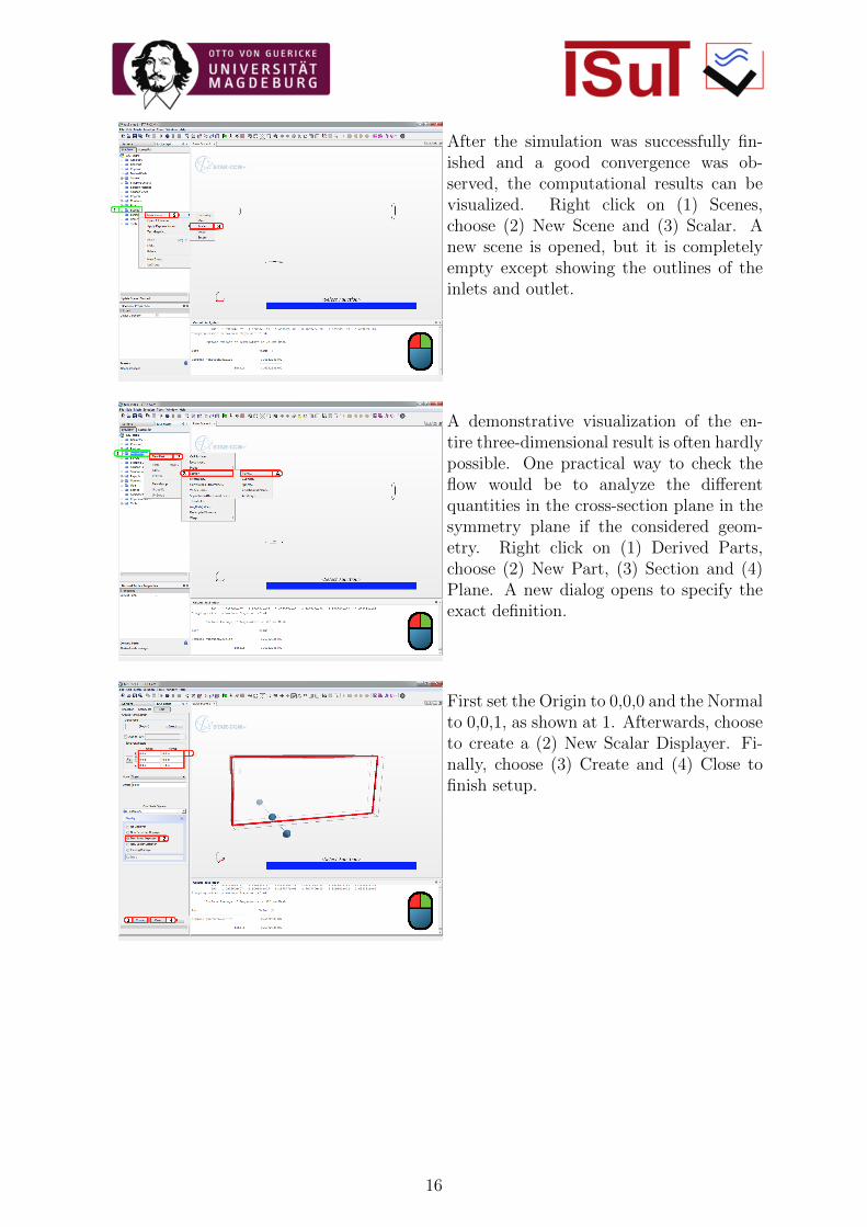
After the simulation was successfully fin-ished and a good convergence was ob-served, the computational results can bevisualized. Right click on (1) Scenes,choose (2) New Scene and (3) Scalar. Anew scene is opened, but it is completelyempty except showing the outlines of theinlets and outlet.

A demonstrative visualization of the en-tire three-dimensional result is often hardlypossible. One practical way to check theflow would be to analyze the differentquantities in the cross-section plane in thesymmetry plane if the considered geom-etry. Right click on (1) Derived Parts,choose (2) New Part, (3) Section and (4)Plane. A new dialog opens to specify theexact definition.

First set the Origin to 0,0,0 and the Normalto 0,0,1, as shown at 1. Afterwards, chooseto create a (2) New Scalar Displayer. Fi-nally, choose (3) Create and (4) Close tofinish setup.

16

Now the contour style is to be changed andthe mesh could be displayed in this cross-section. Click on (1) Section Scalar 1 (toaccess the tree, you might need to clickon Scene/Plot on the top of the ExplorerWindow instead of Simulation. Addition-ally, it is highly advised to remove anyother Scalar Displayer from the tree). Inthe Properties Window, enable (2) DisplayMesh and set Contour Style to SmoothBlended.

First the velocity magnitude in this planewill be shown. Click on (1) Scalar Field inthe Section Scalar 1 node, in the Proper-ties window click on (2) Function. A newdialog is opened to access all the availablevariables. Choose (3) Velocity (not Vortic-ity!) and then (4) Magnitude. Finish theselection by clicking (5) OK.

The velocity magnitude field is displayedwith the mesh together in the previouslydefined cross-section plane.

17

Selecting another variable instead of thevelocity magnitude is easily accessible us-ing the Scene graphical representation win-dow. In this Scene right click on the (1)Color Bar, and from the drop-down listchose (2) Temperature (instead of the Ve-locity) as the Scalar function to be dis-played. The cold and warm streams can bewell observed as well as their mixing. Asthe flow is laminar, this mixing is relativlyslow.

In order to facilitate a three-dimensionaldistribution, an isosurface of T = 330 Kwill be added to the scene. While the Sceneis open, in the Explorer Window right clickon (1) Derived Parts, (2) New Part and (3)Isosurface (if the Explorer window showsthe tree corresponding to the Scalar Scene,do not forget to click on ”Simulation” onthe top of the Explorer Window!). A newdialog is opened on the left side to definethe properties of the isosurface.

First click on (1) Select and choose (2)Temperature in the new dialog. Finish theselection by clicking (3) OK! Afterwards,click (4) Query. This will show the min-imal and maximal values of the functionin the domain. Now, set the (5) Isovalueto 330 K. Choose (6) New Geometry Dis-player and finish the setup by clicking (7)Create and (8) Close.

18

The isosurface is shown now, connecting allthe points in the computational geometryhaving the specified constant temperaturevalue. It might help to appreciate wherethe cold and warm fluids meet.

After finishing the analysis and visualiza-tion of the first setup, a slightly differentgeometry will be analyzed assuming thesame physical process. One could of courserepeat the complete setup from the begin-ning, but StarCCM+ offers a convenientand more efficient way. Open the node (1)Geometry and under the 3D-CAD Modelschoose 3D-CAD Model 1. Choose from theDesign Parameters (3) Radius 2 and mod-ify it to 0.015 m in the Properties Win-dow (4). Afterwards, click on (5) Gener-ate Volume Mesh in the toolbar. The newgeometry according to this value, the cor-responding mesh and the obtained regionwill automatically be updated. This maytake a couple of minutes.

The previously computed result certainlydoes not fit to the new geometry anymore.Further computation is required, so theStopping Criteria has to be changed to al-low more iterations. Open the node Stop-ping Criteria and click (1) Maximum Steps.Set the (2) Maximum Steps to 400 in theProperties Window. Open the node Plotsand double click on (3) avg temp MonitorPlot to open the corresponding plot tab.Additionally, make sure, that the ScalarScene is opened by double clicking on (4)Scalar Scene 1 under the Scenes node. Itwill allow a realtime visualization duringthe computation (but it will certainly besomewhat slower, compared to the previ-ous computation).

19

Click (1) Run to finish the simulation ofthe new setup. You can see, as the Resid-uals jump up due to the modified configu-ration, but shows a convergence soon. Theaveraged temperature at the outlet will bestabilized at a different value, because ofthe difference in the inlet diameters of thedifferent configurations.

20