HANDOVER ALGORITHMS FOR MOBILE IPv6 A THESIS …

HANDOVER ALGORITHMS FOR MOBILE IPv6

A THESIS SUBMITTED TO

THE GRADUATE SCHOOL OF NATURAL AND APPLIED SCIENCES

OF

THE MIDDLE EAST TECHNICAL UNIVERSITY

BY

VEHBİ ÇAĞRI GÜNGÖR

IN PARTIAL FULFILMENT OF THE REQUIREMENTS FOR THE DEGREE OF

MASTER OF SCIENCE

IN

THE DEPARTMENT OF ELECTRICAL AND ELECTRONICS ENGINEERING

DECEMBER 2003

Approval of the Graduate School of Natural and Applied Sciences

____________________

Prof. Dr. Canan Özgen Director

I certify that this thesis satisfies all the requirements as a thesis for the degree of

Master of Science.

____________________

Prof. Dr. Mübeccel Demirekler Head of Department

This is to certify that we have read this thesis and that in our opinion it is fully

adequate in scope and quality, as a thesis for the degree of Master of Science.

____________________

Assoc. Prof. Dr. Buyurman Baykal

Supervisor

Examining Committee Members

Prof. Dr. Hasan Güran ____________________

Prof. Dr. Semih Bilgen ____________________

Assoc. Prof. Dr. Buyurman Baykal ____________________

Assist. Prof. Dr. Cüneyt Bazlamaçcı ____________________

Ilgaz Korkmaz (M.Sc.) ____________________

iii

ABSTRACT

HANDOVER ALGORITHMS FOR MOBILE IPv6

Güngör, Vehbi Çağrı

M.S., Department of Electrical and Electronics Engineering

Supervisor: Assoc. Prof. Dr. Buyurman Baykal

December 2003, 86 pages

With recent technological advances in wireless communication networks, the

need for an efficient architecture for IP mobility is becoming more apparent.

Enabling IP mobility architecture is a significant issue for making use of various

portable devices appearing on the Internet. Mobile IP, the current standard for IP

based mobility management, is capable of providing wireless Internet access to

mobile users. The most important feature of Mobile IP is its ability to support the

changing point of attachment of the mobile user by an algorithm known as

handover. A handover algorithm is needed to maintain connectivity to the Internet

whenever the mobile users move from one subnet to another, while simultaneously

iv

providing minimum disruption to ongoing sessions. This thesis gives an overview of

Mobile IP, its open issues, some of the subsequent enhancements and extensions

related to the handover management problem of the mobile user. Description and

evaluation of various handover algorithms for Mobile IP which have been proposed

to reduce packet loss and delay during handover constitute the core of the thesis. In

this thesis, a comparative performance evaluation of the proposed protocols and the

combination of them is also presented through simulations.

Keywords: Wireless Internet, Mobility Management, Handover Management,

Mobile IP, Mobile QoS

v

ÖZ

MOBILE IPv6 İÇİN HÜCRE DEĞİŞİMİ ALGORİTMALARI

Güngör, Vehbi Çağrı

Yüksek Lisans, Elektrik ve Elektronik Mühendisliği Bölümü

Tez Yöneticisi: Doç. Dr. Buyurman Baykal

Aralık 2003, 86 sayfa

Kablosuz iletişim ağlarındaki teknolojik gelişmelerle birlikte etkili hareketli

IP mimarilerinin gerekliliği daha da açık ortaya çıkmaktadır. İnternetteki çeşitli

taşınabilir araçların kullanımı için hareketli IP mimarilerini mümkün kılmak önemli

bir konudur. Günümüzdeki IP tabanlı hareketlilik yönetimi standardı olan Mobile IP

hareketli kullanıcılar için kablosuz internet erişimi sağlamaktadır. Mobile IP’ nin en

önemli özelliği hareketli kullanıcının yer değiştirmesini hücre değişimi algoritması

sayesinde desteklemesidir. Hücre değişimi algoritması, hareketli kullanıcı bir ağdan

diğer bir ağa hareket ederken internet erişiminin sürekliliği ve bu esnada en az veri

kaybı için gereklidir. Bu tez, Mobile IP’ nin temel özelliklerine, problemlerine,

hareketli kullanıcının hücre değişimi yönetimi ile ilgili gelişmelere ve ilavelere

vi

değinmektedir. Hücre değişimi sırasındaki gecikmeyi ve veri kaybını azaltmak için

öne sürülen Mobile IP’nin hücre değişimi algoritmalarının anlatımı ve

değerlendirilmesi bu tezin özünü oluşturmaktadır. Bu tezde, öne sürülen

protokollerin ve bu protokollerin birleşiminin karşılaştırmalı performans

değerlendirmesi simülasyonlarla ayrıca sunulmaktadır.

Anahtar Kelimeler: Kablosuz İnternet, Hareketlilik Yönetimi, Hücre Değişimi

Yönetimi, Mobile IP, Gezgin Servis Kalitesi

vii

ACKNOWLEDGMENTS

I am very grateful to Assoc. Prof. Dr. Buyurman Baykal for his endless

support and encouragement at all stages of my thesis. I would also like to express

my appreciation to him because of his valuable suggestions, guidance and

experience in solving problems at the critical stages of the thesis, where I gave way

to despair.

Special thanks to ASELSAN Inc. for facilities provided for the completion

of this thesis. I would like to thank to my colleagues for giving me courage to finish

this thesis.

Finally, I would like to express my deep gratitude to my mother Ayten, for

her patience, continuous support and encouragement throughout this thesis.

viii

To my mother,

ix

TABLE OF CONTENTS

ABSTRACT ........................................................................................................ iii

ÖZ ..........................................................................................................................v

ACKNOWLEDGMENTS................................................................................. vii

TABLE OF CONTENTS....................................................................................ix

LIST OF FIGURES.......................................................................................... xiii

LIST OF ABBREVIATIONS...........................................................................xiv

CHAPTER

1. INTRODUCTION.........................................................................................1

2. MOBILE IP OVERVIEW AND MOBILITY MANAGEMENT.............5

2.1. The Need For Mobile IP ........................................................................6

2.2. What is Mobile IP?.................................................................................7

2.3. Terminology in Mobile IP......................................................................7

2.4. Operation Of Mobile IP .........................................................................8

2.5. Basic Mechanisms Of Mobile IP .........................................................10

2.5.1. Agent Discovery ...........................................................................11

2.5.2. Registration...................................................................................12

2.5.3. Tunneling......................................................................................13

2.6. Mobile IP with Route Optimization....................................................13

2.7. Comparison of Mobile IPv6 and Mobile IPv4 ...................................15

2.8. Open Issues in Mobile IPv6 .................................................................16

x

2.9. Mobility Management ..........................................................................17

2.9.1. Location Management ..................................................................19

2.9.2. Handover Management.................................................................20

2.9.2.1. Handover Phases ..............................................................20

2.9.2.2. Handover Types ...............................................................21

2.9.2.3. Handover Requirements ...................................................23

2.9.2.4. Handover Performance Issues ..........................................23

2.9.2.5. Handover Management Techniques in the Literature ......24

3. DESCRIPTION OF HANDOVER ALGORITHMS FOR MIPv6.........26

3.1. IETF and The Standardization Process .............................................27

3.2. Hierarchical Mobile IPv6 ....................................................................28

3.2.1. Mobile IPv6 Extensions in Hierarchical Mobile IPv6..................30

3.2.2. Modes of Hierarchical Mobile IPv6 .............................................31

3.2.3. Mobile Anchor Point Selection in Hierarchical Mobile IPv6 ......32

3.2.4. Evaluation of Hierarchical Mobile IPv6.......................................32

3.3. Fast Handover for Mobile IPv6 ..........................................................34

3.3.1. Anticipated Fast Handover ...........................................................34

3.3.1.1. Anticipated Fast Handover Types ....................................36

3.3.1.2. Anticipated Fast Handover Operation..............................37

3.3.2. Tunnel Based Fast Handover........................................................40

3.3.3. Evaluation of Fast Handover for Mobile IPv6 .............................42

3.4. Simultaneous Bindings for Mobile IPv6.............................................42

3.4.1. Evaluation of Simultaneous Bindings for Mobile IPv6................44

3.5. Combined Handover Algorithm .........................................................45

3.5.1. Combined Handover Operation....................................................45

3.5.2. Evaluation of Combined Handover Algorithm.............................48

4. MODELING OF NETWORK TRAFFIC AND USER MOBILITY .....51

4.1. Modeling of Network Traffic...............................................................51

4.2. Modeling of User Mobility...................................................................54

xi

5. SIMULATION EXPERIMENTS ..............................................................57

5.1. Measurement Methods for Modeling the Link Delay.......................59

5.1.1. Ping ...............................................................................................59

5.1.2. Traceroute .....................................................................................59

5.1.3. One Way Delay Protocol ..............................................................60

5.2. Measurement Method Used in the Thesis ..........................................60

5.2.1. Modeling The Channel Delay in Wired Links .............................61

5.2.2. Modeling The Channel Delay in Wireless Links .........................66

5.3. Modeling Of Traffic Generation And User Mobility ........................66

5.4. Performance Results ............................................................................67

5.5. Comparison of Performance Results and Other Studies..................71

6. CONCLUSIONS AND FUTURE WORK ................................................73

REFERENCES................................................................................................77

xii

LIST OF TABLES

TABLE

2. 1 Cellular coverage division..................................................................................19

5. 1 Node Locations ..................................................................................................60

5. 2 Route Statistics...................................................................................................63

5. 3 Simulation Models .............................................................................................66

5. 4 Performance Results Using Generalized Gamma CRT and Poisson Arrival ....68

5. 5 Performance Results Using Generalized Gamma CRT , Self Similar Traffic ...68

5. 6 Handover Delays................................................................................................68

5. 7 Performance Results in [82]...............................................................................71

5. 8 Performance Results in [83]...............................................................................71

xiii

LIST OF FIGURES

FIGURE

2. 1 A high level picture of Mobile IP protocol .......................................................10

2. 2 Message flow during registration procedure in Mobile IP................................12

2. 3 Network Layered Model ...................................................................................17

2. 4 Mobility Management.......................................................................................19

2. 5 Handover Types ................................................................................................20

3. 1 The packet flow during HMIPv6 handover ......................................................30

3. 2 Anticipated Fast Handover Types.....................................................................37

3. 3 Message flow during Fast Handover.................................................................38

3. 4 The message flow between the oAR and the nAR............................................39

3. 5 Message flow during Mobile Initiated and Stateless Fast Handover................40

3. 6 Handover to third scenario for Tunnel Based Handover ..................................41

3. 7 Bicasting Simultaneous Binding Function........................................................43

3. 8 N-casting Simultaneous Binding Function .......................................................44

3. 9 Message flow of combined handover algorithm during handover....................48

4. 1 Pictorial proof of self-similarity: Ethernet traffic on 5 different scales ............53

5. 1 Simulation Network Topology..........................................................................58

xiv

5. 2 The measurement architecture for modeling the wired link delay....................61

5. 3 The Node map for path 4 (Aselsan-METU link) ..............................................62

5. 4 The Node map for path 5 (Aselsan-MIT link) ..................................................62

5. 5 The shifted Gamma fitted curve for path 4 .......................................................64

5. 6 The shifted Weibull fitted curve for path 4.......................................................64

5. 7 The shifted Gamma fitted curve for path 5 .......................................................65

5. 8 The shifted Weibull fitted curve for path 5.......................................................65

5. 9 The measurement architecture for modeling the wireless link delay................66

5. 10 Comparison of Algorithms (1 packet/msec Poisson arrival) ..........................69

5. 11 Comparison of Algorithms (0.1 packet/msec Poisson arrival) .......................69

5. 12 Comparison of Algorithms (0.05 packet/msec Poisson arrival) .....................70

5. 13 Comparison of Algorithms (Self Similar Traffic)...........................................70

xv

LIST OF ABBREVIATIONS

3G 3rd Generation

4G 4th Generation

aAR anchor Access Router

AP Access Point

AR Access Router

BACK Binding Acknowledgment

BETH Bidirectional Edge Tunnel Handover

BP Beacon Period

BU Binding Update

CN Correspondent Node

CCoA Co-Located Care of Address

CoA Care of Address

CRT Cell Residence Time

FA Foreign Agent

DHCP Dynamic Host Configuration Protocol

Fast MIPv6 Fast Handover for Mobile IPv6

F-Back Fast Binding Acknowledgment

F-BU Fast Binding Update

xvi

F-NA Fast Neighbor Advertisement

GRE Generic Routing Encapsulation

HA Home Agent

HAck Handover Acknowledgment

HMIPv6 Hierarchical Mobile IPv6

HI Handover Initiate

HTT Handover To Third

ICMP Internet Control Message Protocol

I-D Internet Draft

IRTF Internet Research Task Force

IESG Internet Engineering Steering Group

IETF Internet Engineering Task Force

IP Internet Protocol

IPPM IP Performance Metrics

IPsec IP security

IPv4 IP version 4

IPv6 IP version 6

LANs Local Area Networks

LCoA Link care of address

LRD Long Range Dependent

MAN Metropolitan Area Network

MAP Mobility Anchor Point

xvii

MD-5 Message Digest-5

MN Mobile Node

MIPv4 Mobile IPv4

MIPv6 Mobile IPv6

nAR new Access Router

nCoA new Care of Address

oAR old Access Router

oCoA old Care of Address

PDA Personal Digital Assistant

PPP Point to Point Protocol

PrRtAdv Proxy Router Advertisement

QoS Quality of Service

OWDP One-way Delay Protocol

RFC Request For Comments

RCoA Regional care of address

RtAdv Router Advertisement

RtSol Router Solicitation

RtSolPr Router Solicitation Proxy

RTT Round Trip Time

TCP Transport Control Protocol

TTL Time To Live

UDP User Datagram Protocol

xviii

UML Unified Modeling Language

WANs Wide Area Networks

WWW World Wide Web

1

CHAPTER 1

INTRODUCTION

The recent developments in wireless communication technology and the

rapid growth of the Internet have paved the way for wireless Internet and IP

mobility. Various portable computing devices ranging from laptops, handheld

computers to other personal digital assistants (PDAs) with networking capabilities

increase the demand for seamless communication both in wired and wireless

network architectures. Increased use of real time applications and multimedia

services on mobile terminals makes seamless communication an essential feature

expected in future mobile communication systems.

The demand for mobile computing, so called “anytime/anywhere”

computing, together with high level service quality is expected to ever proliferate in

the near future. The range of application types that the mobile users of future

wireless networks expect and the variety of QoS specifications that they require

from mobile computing environments will grow drastically. The rapidly increasing

demand for “anytime/anywhere” high speed Internet access will be one of the major

forthcoming challenges for mobile networks operators [1]. As the need for mobility

increases, the ability to connect mobile terminals, from laptops and PDAs to future

mobile videophones and other future devices to the Internet and Intranets and

achieve service quality levels just as stationary users will have become mandatory in

the future wireless networks.

2

While the wireless network service providers are responsible for providing a

broad range of applications and high levels of service quality to mobile hosts, they

must also overcome some difficulties coming from the nature of wireless

environments. Unlike conventional wired networks, wireless networks possess

different channel characteristics. The main problem in wireless networks is that the

channel capacity typically available is much lower than that of wired networks due

to the noise levels and power restrictions.

Apart from these inevitable problems of wireless networks, mobility also

brings about some additional constraints which make network design and analysis

more challenging. Wireless mobile users can be connected to the Internet by using

Access Points (AP) in IP networks. However due to roaming, these users may

change its AP each time they move from one cell, that is coverage area of AP, to

another. This cell boundary crossing movement during the active connection period

is called handover. The handover algorithm should exhibit low delay and cause

reasonable or no data loss in order to maintain connectivity as the mobile users

move. Otherwise, the active call might be blocked.

The increasing variety of wireless devices offering network connectivity has

actually revolutionized the way people access information. In fact, these advances

have given birth to the era of the wireless Internet. Integrating wireless networks

into the global Internet poses a new challenge [2]. The main reason is that the

TCP/IP based Internet technologies were designed for wired networks with mostly

fixed hosts. Host mobility requires changes in the routing protocol so that packets

for a moving host can be delivered to their correct destination. Mobile IP [3]

provides a basic framework to solve this operability problem, with the assumption

that there is enough infrastructure support so that a mobile node (MN) can

communicate with an AP, which is statically connected to the Internet.

Mobile IP defines mechanisms for supporting MNs in communication

networks. It works by using two IP addresses for each MN: A static home IP

address for mobile host identification purposes and a variable dynamic care of IP

3

address (CoA) for routing purposes. In this way, when a MN moves to another

home network, it will still be able to communicate with other hosts.

When a MN changes its point of attachment, a handover is initiated. A

handover typically involves the process of discovering new point of attachment,

obtaining a new CoA and informing the new CoA to other nodes in order to ensure

correct routing. During handover, while the MN is still in the process of obtaining

and registering a new CoA, packets addressed to the MN may be lost by being

delivered to its old CoA. Packet loss will be significant especially when the

handover latency is long. This is a major problem since it will degrade the

communication performance and the mobile user may experience slower connection

or permanent loss of packets depending on the type of application. Mobile Internet

users expect to maintain continuous connection to the Internet, without any

communication interruptions or performance degradation during motion. In other

words, handovers must be seamless, i.e. they must be transparent to the mobile user.

Ideally, the Mobile IP performance over wireless devices should be equivalent to IP

performance in wired networks.

Mobile IP, an extension to the existing IP protocol, has essentially two

versions, i.e. Mobile IPv4 (MIPv4) and Mobile IPv6 (MIPv6) corresponds to the old

and new versions of IP respectively. This thesis mainly focuses on MIPv6. In order

to achieve seamless handover in MIPv6, several handover mechanisms have been

proposed which tend to reduce the handover latency and packet loss. This thesis

describes some of the main seamless handover algorithms in MIPv6. The algorithms

proposed to enhance the performance of MIPv6 are Hierarchical MIPv6 [4], Fast

Handover for MIPv6 [5], Simultaneous Bindings for MIPv6 [6]. The proposed

protocols try to solve the problem of the service disruption during MIPv6 handover

with different methods each. However, these protocols have also some drawbacks

and a possible combination of them is necessary in order to enhance the MIPv6

protocol. In addition, since the proposed handover algorithms are quite new, there

have not been enough research and evaluation done on these algorithms. Therefore,

a proper performance evaluation of these algorithms either by simulations or test

4

beds is of great importance for design issues. The performance evaluations can then

be used to improve these methods further.

In this thesis, the appropriate combination of the extensions is also presented

and the detailed performance evaluation of the handover schemes and the combined

handover method is carried out through simulations. In order to properly predict the

performance of handover extensions of MIPv6, the user mobility, the network

traffic, wired and wireless links in the simulated network topology are modeled

through stochastic processes. Firstly, the network traffic is modeled by both

traditional framework modeling (termed Poisson modeling) and self similar traffic

modeling [7]. Secondly, the user mobility is modeled by assuming that cell

residence time of the mobile user exhibits generalized gamma distribution [8].

Thirdly, the links in simulation network architecture are modeled from real traces

taken on the Internet between April and August of 2003.

Following this introduction in Chapter I, the rest of this thesis is organized as

follows. In Chapter II, the main Mobile IP mechanisms and some open issues are

introduced and the mobility management issues at the network layer are discussed.

Chapter III describes the proposed handover algorithms and combined handover

method in detail. In Chapter IV, network traffic and user mobility modeling is

discussed. Chapter V shows the results of the comparative simulation experiments.

Finally, conclusions and future work are presented in Chapter VI.

5

CHAPTER 2

MOBILE IP OVERVIEW AND MOBILITY MANAGEMENT

In response to the increasing variety and popularity of wireless devices

offering network connectivity, Mobile IP was developed to enable mobile users to

maintain Internet connectivity while moving from one Internet attachment point to

another. Although Mobile IP can work with wired connections, in which a computer

is unplugged from one physical attachment point and plugged into another, it is

particularly appropriate for wireless connections [9].

The term mobile in this thesis implies that the user, connected to some sort

of application across the Internet, changes its point of attachment dynamically and

that all the required reconnections are maintained automatically and

noninteractively. Consequently, mobile computing should not be confused with

portable or nomadic computing. Also, incorporating mobility into broadband

systems requires many considerations in every layer of the communication [10]. For

instance, power control in the physical layer, traffic management in the data link

layer, mobility management in the network layer and communication optimizations

in the transport and application layer.

6

2.1. The Need For Mobile IP

Traditional IP networks are based on the assumption that the network

infrastructure is fixed. The Internet Protocol (IP) also supposes that the physical

location of the computers do not change while it is connected to the network. In

other words, the location of the user connected to the network is assumed to be fixed

so that it is assigned a fixed IP address. However, all these assumptions seem to

disappear once the user becomes a mobile one. In a mobile computing environment,

the user should be able to connect to the network from different access points

through wireless links and the network should be capable of keeping the mobile user

connected while it moves to another network and changes its point of attachment.

In order to maintain connectivity to the Internet in a mobile environment, the

following operations might be employed:

• Whenever the mobile user moves to a new subnet, it changes its IP address

to reflect the new point of attachment.

• The routers keep host specific routes for the mobile node.

Both these alternatives can not be applicable due to their drawbacks.

Changing the IP address seen by the transport and the application layers every time

a mobile user moves to a new network might be a solution to infrequent roaming,

but not to mobility in general. The main reason is that the transport layer, e.g. TCP,

uses the IP address as an identifier to correlate IP packets to transport sessions. If

the corresponding IP address changes, then the correlation is lost and the sessions

need to be restarted [11]. Therefore, in order to maintain existing transport layer

connections, the mobile user should keep its IP address the same while moving. The

other alternative, that is host specific routes, in general can not be scalable for the

widespread Internet use.

In order to solve IP mobility problem, Mobile IP standard was proposed. The

general overview of Mobile IP will be given in the following sections.

7

2.2. What is Mobile IP?

Mobile IP ([3], [12]), proposed by the Internet Engineering Task Force

working group, is a modification to IP that enables nodes to change their points of

attachments to the Internet without changing their IP addresses. Mobile IP is

essentially a network layer solution which is intended to be transparent to all upper

layer protocols.

Mobile IP accomplishes its task by setting up IP routing tables in

appropriate nodes so that IP packets destined to mobile hosts can be reachable.

Control messages, defined in Mobile IP, allow IP nodes involved to manage their IP

routing tables reliably. The primary purpose of Mobile IP is to allow IP packets to

be routed to mobile nodes which could potentially change their location

continuously.

2.3. Terminology in Mobile IP

Mobile IP defines the following functional entities [9], which will be used

across the thesis to describe the mechanisms of Mobile IP:

• Mobile Node (MN): A mobile node is an Internet node or a host which can

change its point of attachment to the Internet from one network or

subnetwork to another while maintaining any ongoing sessions.

• Home Agent (HA): A home agent is a router on a mobile node’s home

network which tunnels datagrams for delivery to the mobile node when it is

away from home. It also maintains current location information for the

mobile node.

• Foreign Agent (FA): A foreign agent is a router on a mobile node’s visited

network which provides routing services to the mobile node while

registered. This entity detunnels datagrams coming from the home agent and

destined to the mobile host.

• Correspondent Node (CN): A correspondent node is a node that

communicates with the mobile node.

8

• Home Network: A Home network is the network having a network prefix

matching that of mobile node’s home address.

• Foreign Network: A foreign network is any network other than the mobile

node’s home network.

• Visited Network: A visited network is the network at which a mobile node

is currently connected. It is also a foreign network.

• Home Address: A home address of a mobile node is an IP address which

has been assigned to the mobile node permanently. This home address does

not change when the mobile node moves from one subnet to another in the

home network. The home address of the mobile node only changes, when it

moves from one home network to another.

• Care of Address (CoA): A care of address is an IP address for the foreign

agent. When the mobile node is away from its home network, IP packets

intended for the mobile node are encapsulated and forwarded to this address.

• Co-Located Care of Address (CCoA): In some cases, a mobile node may

move to a network that has no foreign agents or on which all foreign agents

are busy. As an alternative, the mobile node may act as its own foreign agent

by using a co-located address. A co-located care of address is an IP address

obtained by the mobile node that is associated with the mobile node’s

current interface to a network. The means by which a mobile node acquires a

co-located address is beyond the scope of Mobile IP. One means is to

dynamically acquire a temporary IP address through an Internet service such

as Dynamic Host Configuration Protocol (DHCP).

2.4. Operation Of Mobile IP

Mobile IP solves the problem of IP mobility by assigning two IP addresses

to each mobile node (MN). The first IP address is the home address, which is a

static and permanent address used to identify the mobile node globally. Home

address is also essential for the MN to maintain a constant TCP connection. Every

9

MN is associated with a home network, which provides the home address. At the

home network, there is a special router called the Home Agent (HA), which stores

the home address of the MN and keeps track of the MN location as it moves. When

a mobile node attaches to a foreign network, it obtains the second temporary IP

address called care of address (CoA), which provides information about the MN’s

current location. The MN registers this new CoA with its HA in order to track the

MN’s current location. This process, that is mapping or association between the

current care of address and the home address, is called binding. The HA is then

responsible for intercepting packets addressed to the MN and forwarding them to

the CoA of the MN by a mechanism known as tunneling.

Furthermore, Mobile IP introduces entities called Foreign Agents (FA)

located at foreign networks. A FA is responsible for cooperating with the home

agent of a mobile node to deliver packets to the mobile node successfully. Their

major functionality is to detunnel packets addressed to a MN and deliver them to the

MN. A FA is also responsible for advertising available CoA addresses. In some

situations, it is possible that a MN may move to a network where no FA is available.

In this case, the MN may obtain a CoA from a Dynamic Host Configuration

Protocol (DHCP) server or a Point to Point Protocol (PPP). This type of CoA

address is called co-located care of address (CCoA). To support CCoA, a MN must

have the ability to detunnel packets arriving from the HA.

Figure 2.1 illustrates the basic mobility support mechanism of Mobile IP.

When a Corresponding Node (CN) wants to send packets to a mobile node MN, it

identifies the MN by its home address and sends the packets to the home address of

the MN. The source address of these packets is the CN address, while the

destination address is the home address of the MN. If the MN has moved to a

foreign network, the HA intercepts the packets addressed to the MN. The HA has a

binding cache listing the CoA of all the nodes in the home network which are

currently at visited networks. Based on its binding cache, the HA “tunnels” these

packets to the CoA of the MN. Tunneling is done by encapsulating the original

datagrams within other datagrams (IP- within- IP encapsulation), with the source

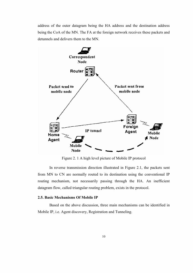
10

address of the outer datagram being the HA address and the destination address

being the CoA of the MN. The FA at the foreign network receives these packets and

detunnels and delivers them to the MN.

Figure 2. 1 A high level picture of Mobile IP protocol

In reverse transmission direction illustrated in Figure 2.1, the packets sent

from MN to CN are normally routed to its destination using the conventional IP

routing mechanism, not necessarily passing through the HA. An inefficient

datagram flow, called triangular routing problem, exists in the protocol.

2.5. Basic Mechanisms Of Mobile IP

Based on the above discussion, three main mechanisms can be identified in

Mobile IP, i.e. Agent discovery, Registration and Tunneling.

11

2.5.1. Agent Discovery

A mobile node uses an agent discovery procedure to identify prospective

home agents and foreign agents. Mobile agents, i.e. Home Agent and Foreign

Agent, advertise their presence by broadcasting Agent Advertisement messages at

regular intervals. These agent advertisement messages are an extension of the

standard ICMP (Internet Control Message Protocol) Router Advertisement [13]

messages. The source IP address in the advertisement message is used by the MN to

determine if it is still linked to the home network. If the network prefix of the source

address in the IP header of the advertisement message is equal to the network prefix

of the MN’s home address, then the MN decides that it is still linked to its home

network. Otherwise, the MN assumes that it is on a foreign network and thus

proceeds to get a CoA from the FA at the visited network. In case a mobile node

needs agent information immediately, it can issue an ICMP agent solicitation

message. Any agent receiving this message will then issue an agent advertisement.

As mentioned, a mobile node may move from one network to another due to

some handover mechanism, without the IP level being aware of it. The agent

discovery process is intended to enable the agent to detect such a move. The agent

may use one of two following algorithms for this purpose:

1) Use of life time field: When a MN receives an agent advertisement from a

FA that it is currently using or that it is now going to register with, it records

the lifetime as a timer. If the timer expires before the agent receives another

agent advertisement from the agent, then the node assumes that it is lost

contact with that agent. In the mean time, if the MN has received an agent

advertisement from another agent and that advertisement has not yet expired,

the MN can register with this new agent. Otherwise, the mobile node should

use agent solicitation to find an agent.

2) Use of network prefix: The mobile node checks whether any newly

received agent advertisement is on the same network as the MN’s current

12

care of address. If it is not, the MN assumes that it has moved and may

register with the agent whose advertisement the MN has just received.

2.5.2. Registration

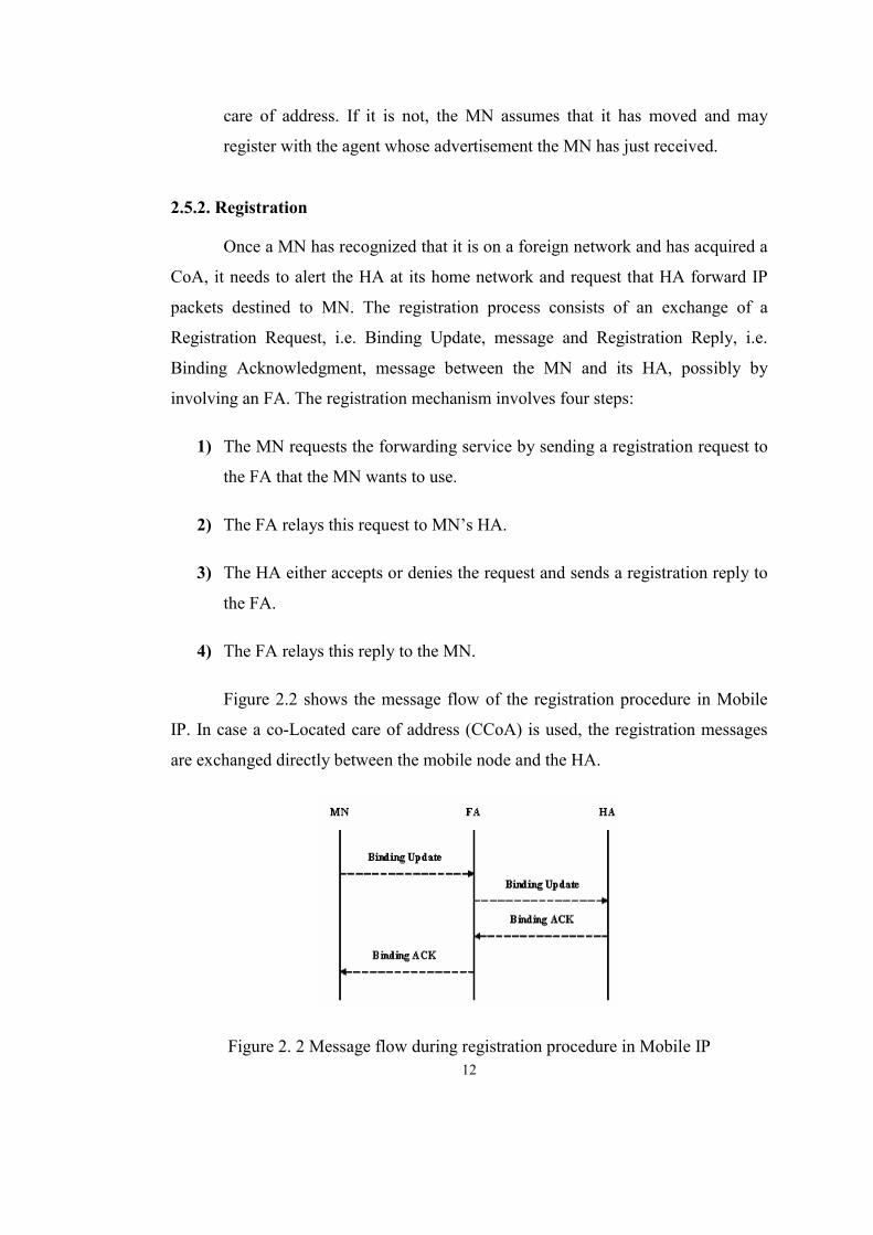
Once a MN has recognized that it is on a foreign network and has acquired a

CoA, it needs to alert the HA at its home network and request that HA forward IP

packets destined to MN. The registration process consists of an exchange of a

Registration Request, i.e. Binding Update, message and Registration Reply, i.e.

Binding Acknowledgment, message between the MN and its HA, possibly by

involving an FA. The registration mechanism involves four steps:

1) The MN requests the forwarding service by sending a registration request to

the FA that the MN wants to use.

2) The FA relays this request to MN’s HA.

3) The HA either accepts or denies the request and sends a registration reply to

the FA.

4) The FA relays this reply to the MN.

Figure 2.2 shows the message flow of the registration procedure in Mobile

IP. In case a co-Located care of address (CCoA) is used, the registration messages

are exchanged directly between the mobile node and the HA.

Figure 2. 2 Message flow during registration procedure in Mobile IP

13

Another important point in the registration procedure is security. Mobile IP

is developed to manage two types of attacks:

1) A node may pretend to be a FA and send a registration request to HA in

order to direct the traffic intended for a MN to itself.

2) A malicious agent may replay old registration messages, effectively cutting

the MN from the network.

The technique that is used to protect against such attacks involves the use of

message authentication and the proper use of identification field of the registration

request and reply messages. The default authentication method n Mobile IP is keyed

MD-5 algorithm [14].

2.5.3. Tunneling

Tunneling is the mechanism by which the HA forwards the packets to the

MNs. Using this mechanism, the IP packets are placed within the payload part of

new IP packets, and the destination address of the encapsulating, i.e. outer, IP

header is set to the MN’s CoA. Upon reception of each IP packet, the FA

decapsulates it by removing the outer IP packet and sends the original packet to the

MN. Three options for encapsulation are suggested for Mobile IP:

• IP-within-IP encapsulation: This is the simplest approach, defined in [15].

• Minimal encapsulation: This approach involves fewer fields, defined in

[16].

• Generic Routing Encapsulation (GRE): This is a generic encapsulation

procedure that was developed prior to the development of Mobile IP, defined

in [17].

2.6. Mobile IP with Route Optimization

Although the packets sent from the CN to the MN must pass through the HA

when the MN is away from the home network, the packets from the MN to the CN

14

can still be routed directly to their destinations. This asymmetric routing, as shown

in Figure 2.1, is called triangular routing problem. Mobile IP suffers from triangle

routing problem especially in cases when the CN is very close to the MN. Route

optimization solves the triangle routing problem by introducing changes in the CN.

Standard route optimization [18] is used for optimizing the routing of

packets from the CN to the MN. This is achieved by improving the CN so that it has

a binding cache associated with the MN. Once the CN creates a binding for a

particular MN, this binding must be updated in order to ensure correct routing. With

updated binding, the CN will be able to send encapsulated datagrams directly to the

MN instead of sending it to the HA of the MN. It is also noted that the enhanced CN

must now be capable of encapsulating datagrams on behalf of the HA.

The main issue in route optimization is to update the binding at the CN.

Binding update messages are used for sending updated CoA of the MN to the CN.

Typically, the HA is responsible for sending the binding updates. When the CN

communicates with the MN for the first time via the HA, the HA will automatically

send a binding update to the CN to inform the CN of the MN’s CoA. In certain

cases, to ensure fast binding update as the MN obtains a new CoA, the MN may

send a binding update directly to the CN. In this case, the MN can request a binding

acknowledgment from the CN. The HA does not request binding acknowledgment

from the CN since it can understand whether the binding update has not been

received by the CN if it receives datagrams destined to the MN from that CN.

In standard route optimization, it is assumed that the traffic from the MN to

the CN can be routed directly to the CN without having to pass through the HA of

the MN. In this case, the source address of the packets is the home address of the

MN, while the destination address is the IP address of the CN. However, this direct

routing mechanism is not always possible. This is because some networks utilize

ingress filtering routers [19] which drop packets whose source address is not

topologically correct. Standard route optimization suggests that the reverse path

from the MN to the CN is a direct route, i.e. ingress filtering routers are ignored.

15

2.7. Comparison of Mobile IPv6 and Mobile IPv4

Mobile IP was originally defined for IP version 4 (IPv4) [3], before IP

version 6 (IPv6) existed. Mobile IPv4 (MIPv4) and Mobile IPv6 (MIPv6) protocols

share similar ideas, but their implementations are somewhat different. IP mobility is

also specified for IPv4, but IPv6 provides more enhanced support for it. The major

differences between MIPv4 and MIPv6 are as follows:

• The address space of MIPv6 is bigger than that of MIPv4. IPv6 header is

divided into optional extension headers. This makes the IPv6 base header

smaller and more efficient for routers to route. The introduction of extension

headers makes it possible to supply more information to the participants

without disturbing parts of the system with information that they do not

need.

• IPv6 address autoconfiguration simplifies the care of address assignment for

the mobile node. It also eases the address management in a large network

infrastructure. To obtain a care of address, the MN can use either stateful or

stateless address autoconfiguration. In the stateful address autoconfiguration,

the MN obtains a care of address from a DHCPv6 (Dynamic Host

Configuration Protocol for IPv6) server. In the stateless address

autoconfiguration, the MN extracts the network prefixes from the Router

Advertisements, i.e. equivalent to Agent Advertisements in MIPv4, and adds

a unique interface identifier to form a care of address.

• In MIPv6 an Advertisement Interval option on Router Advertisements is

defined, that allows a Mobile Node to decide for itself how many Router

Advertisements (Agent Advertisements) it is tolerating to miss before

declaring its current router unreachable.

• Route Optimization feature to avoid triangle routing problem is built in as a

fundamental part of the MIPv6 protocol. In MIPv4 this feature is being

added on as an optional set of extensions that may not be supported by all IP

nodes.

16

• In MIPv6 the functionality of the Foreign Agents can be accomplished by

IPv6 enhanced features, such as Neighbour Discovery [20] and Address

Autoconfiguration [21]. Therefore, there may be no need to deploy Foreign

Agents in MIPv6.

• The Mobile IPv6, unlike Mobile IPv4, uses IPsec ([22], [23] and [24]) for all

security requirements such as sender authentication, data integrity

protection, and replay protection for Binding Updates. In MIPv4, the

security requirements are provided by its own security mechanisms for each

function, based on statically configured mobility security associations.

• MIPv6 and IPv6 use the source routing feature which is the insertion of

routing information into a datagram by the source node. This feature makes

it possible for the CN to send packets to the MN while it is away from its

home network using an IPv6 Routing header rather than IP encapsulation,

whereas MIPv4 must use encapsulation for all packets. However, in Mobile

IPv6 the Home Agents are allowed to use encapsulation for tunneling. This

is required, during the initiation phase of the binding update procedure.

2.8. Open Issues in Mobile IPv6

The good side of the MIPv6 is that it optimizes the routing, because the MN

and the CNs exchange data packets to one another directly after the HA has

informed the CoA to the CNs. Before the CN knows the MN’s CoA the data goes

trough the HA tunneling service. However, despite the route optimization, the

MIPv6 is considered to be badly scalable [25]. As the number of the MNs increase,

the number of Binding Update messages (BUs) increase proportionally. This

phenomenon may end up creating congestions in the network backbone.

When the HA and the MN are far from each other, even small MN

movements create BUs that traverse a long way across the network. Also, the route

optimization, that enables direct data exchange between the MN and the CN,

generates BUs that add overhead to the network, especially with the requirement

that the BUs and corresponding Binding Acknowledgments (BACK) be encrypted

17

with IPsec ([26], [27]). Long message routes might lengthen handover times and

result in QoS deterioration. In case of frequent handovers, the long control traffic

between the MN and the HA causes inefficiency in handover management of the

MN. In order to solve this problem, regional registration using hierarchical mobility

management [4], discussed further in Chapter 3, is proposed.

2.9. Mobility Management

The enormous demands for wireless communication technologies lead to

plenty of new protocols emerging which propose to deliver miscellaneous wireless

services to the mobile users with more excellent quality. Within these protocols,

mobility management is one of the most important problems for a seamless access

to wireless networks and services. It is also the fundamental issue used to

automatically support the mobile users enjoying their services meanwhile

roaming freely without any interruption in their connections. Future mobile

communication systems evolve with the trend of global connectivity through

the internetworking and interoperability of heterogeneous wireless networks.

Mobility in these network architectures is a very complex issue which results in

many new problems. Therefore, the mobility management protocol needs to be

carefully and efficiently designed to provide the requirements of real time and

multimedia applications. It is also important to mention that Mobile IP is a mobility

management protocol which works at the network layer. Moreover, mobility in

wireless communication networks affects every layer of the communication [28], as

shown in Figure 2.3.

Figure 2. 3 Network Layered Model

18

• At the physical layer, the mobility influences are remarkable due to wireless

media characteristics. Resource reuse and interference avoidance are two

important problems at this layer.

• At the data link layer, the mobility in wireless networks brings

problems of bandwidth, security, and reliability. Other problems include

fixed or dynamic channel allocation algorithms, collision detection and

avoidance measures, QoS resource management, etc.

• At the network layer, the mobility of mobile nodes means that new

routing algorithms are needed to change the packets routing. To track

a mobile node’s movement and to keep the moving node’s connectivity

forms two main components of mobility management, i.e. location

management and handover management.

• At the transport layer, an end to end connection of the mobile node may

mix both wired and wireless links. This makes congestion control a

complex task due to the different network characteristics.

Retransmission mechanism based on increasing interval may lead to an

unnecessary drop in the data rate.

• At the application layer, mobility brings new requirements such as service

discovery schemes, QoS, and environment auto configuration. Mobility also

brings new opportunities to applications.

From the cellular structure point of view, future mobile networks can be

divided into different sizes of cellular coverage [28], as shown in Table 2.1.

The basic idea behind this is to seamlessly integrate two categories of wireless

network technologies together, i.e. those that can provide low bandwidth over

a wide geographic area and those that can provide a high bandwidth over a

narrow geographic area.

19

Table 2. 1 Cellular coverage division

Cell Name Place Coverage Speed

Techniques

Mega Cell Global Global Coverage

>200 km/h Satellite

Macro Cell Suburban, Rural

1km -10 km 20-200 km/h 2G/3G

Micro Cell Urban 100m -1km 10-50 km/h WLAN, Hiper LAN

Pico Cell In Building 10m -100m < 10 km/h WLAN, Bluetooth

Nano Cell Personal Area 1m -10m Nearly Stationary

Bluetooth

From the viewpoint of functionality, mobility management mainly

enables communication networks to locate roaming terminals in order to deliver

data packets and to maintain connections with terminals moving into new areas.

In this context, mobility management can be considered as two complementary

components [29], i.e. location management and handover management, as shown in

Figure 2.4.

Figure 2. 4 Mobility Management

2.9.1. Location Management

Location management which provides the network to discover the current

attachment point of the mobile user is a two stage process. The first stage is location

update in which the network is notified the new access point of the mobile user

20

periodically. The second stage is call delivery. In this stage, the current location of

the mobile user is queried in the network.

2.9.2. Handover Management

Handover management is the process of enabling the network to maintain

the mobile user’s connection while the mobile user moves. In this thesis, handover

management is the major issue to be discussed. Therefore, the details of handover

management will be described in the following section.

2.9.2.1. Handover Phases

The handover procedure can be analyzed in three main phases:

• Initiation Phase: Either the mobile user or the network, or both of them

make the decision about the handover initiation. If the handover necessity is

noticed by the mobile user due to deterioration in the received signal

strength, then the mobile user initiates handover process. In cases related to

network management, the network initiates the process.

• Preparation Phase: In order to achieve the requirements imposed by QoS

specifications, the network of the new access point should be prepared for

the active call of the mobile user just after the initiation phase.

• Execution Phase: In this phase, reserved resources are allocated so as to

preserve active calls without any interruption.

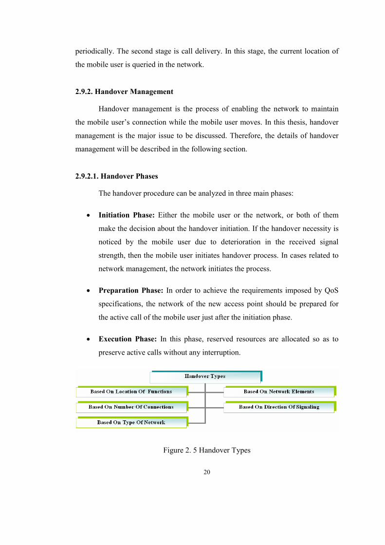
Figure 2. 5 Handover Types

21

2.9.2.2. Handover Types

The handover procedures attempt to maintain the connections of the mobile

user as it moves from one network to another. The classifications of the handover

processes are based on various criteria. These classifications, as shown in Figure

2.5, are described as follows:

• The handover procedures can be classified based on the location of the

handover functions [30]:

a) Mobile Initiated Handover: In this type of handover, the mobile user

has to manage the handover. That is, it takes the measurements on the

downlink, processes them, takes the decision to do the handover and

decides the target access router.

b) Mobile Evaluated Handover: This is similar to the mobile initiated

handover except that the decision to do the handover lies with the

network.

c) Network Initiated Handover: In this type of handover, the network

manages the handover, which includes taking measurements on the

uplink, processing them, deciding to do the handover and deciding the

target access router.

d) Mobile Assisted Handover: This is similar to the network initiated

handover, except that the mobile assists the network by taking

measurements along the downlink and relaying them back to the

network.

• The handover procedure can also be classified based on the network

elements involved in the handover [31]:

a) Intra Cell: This type of handover is done within the current coverage

area, i.e. cell. The used channel, e.g. the time slot, is only changed for

this type of handover.

b) Inter Cell: If the mobile user crosses the cell boundary, then it is

referred to as inter cell handover.

22

c) Inter Network: If the handover is done between two different networks,

then it is referred to inter network handover.

• The handovers can also be classified based on the number of the connections

that a mobile user maintains during the handover procedure [32]:

a) Soft Handover: In this type of handover, the mobile user is connected

simultaneously to two accesses. As it moves from one cell to another, it

“softly” switches from one access router to another. When connected to

two access routers, the network combines information received from two

different routes to obtain a better quality. This is commonly referred to as

macro diversity.

b) Hard Handover: In this type of handover, the mobile user switches the

communication from the old link to the new link. Thus, there is only one

active connection from the mobile user at any time. There is a short

interrupt in the transmission. This interrupt should be minimized in order

to make the handover seamless.

• Another way of classifying the handovers is the direction of the handover

signaling [33]:

a) Forward Handover: After the mobile user decides the cell to which it

will make a handover, it contacts the access router controlling the cell.

The new access router initiates the handover signaling to unlink the

mobile user from the old access router. This is especially useful if the

mobile user suddenly loses contact with the current base station. This is

referred to as forward handover.

b) Backward Handover: After the mobile terminal decides the cell to

which it attempts to make a handover, it contacts the current access

router, which initiates the signaling to do the handover to the new access

router. This is referred to as backward handover.

23

• The handover procedures can also be classified based on the type of the

network [34]:

a) Horizontal Handover: This type of handover refers to handovers

between cells belonging to the same network. That is, the MN moves

within the same network. Horizontal handover also represents a micro

level mobility scenario, i.e. intra network mobility.

b) Vertical Handover: This type of handover refers to handovers between

cells belonging to different types of the network. That is, the MN moves

from one network to another network. Vertical handover also represents

a macro level mobility scenario, i.e. inter network mobility.

2.9.2.3. Handover Requirements

The general requirements [35] for the handover procedure are listed in this

section:

• Handover Delay: The total time for the completion of the handover should

be appropriate for the rate of mobility of the mobile user. That is, the

handover process should be fast so that the mobile user does not experience

service degradation or interruption during handover.

• Scalability: The handover procedure should support seamless and lossless

handover within both the same and different networks. It should also be able

to integrate seamlessly with the existing wired networks.

• Quality of Service (QoS): The effect of the handover on QoS should be

minimal so as to maintain the requested QoS after the handover is

completed.

• Signaling Traffic: The amount of signaling traffic required to make the

handover should be kept to a minimum.

2.9.2.4. Handover Performance Issues

Besides these handover requirements, described above, there are some

performance issues in order to provide uninterrupted services and continuous

communication during handover [36]:

24

• Fast handover: The handover operations should be quick enough to ensure

that the mobile user can receive data packets at its new location

within a reasonable time interval. Reducing the handover latency as much

as possible is extremely important for real time applications.

• Smooth handover: The handover algorithm should minimize the packet

loss, although the interruption time may be long.

• Seamless handover: Combination of fast handover and smooth handover

are sometimes referred to as seamless handover. While the former concerns

mainly packet delay, the latter focuses more on packet loss. In certain cases,

seamless handover may be impossible. For example, if the mobile user

moves among networks where the coverage areas of the two access points do

not overlap, there will be a discontinuity which will cause interruption and

packet loss.

2.9.2.5. Handover Management Techniques in the Literature

Some distinct but complementary techniques exist for handover

management:

• Buffering and forwarding: During the handover procedure, the old or new

attachment point of the mobile node can store packets and then forward to

the mobile node or the new attachment point of the mobile node. This type

of technique is used in [5] and [6].

• Movement detection and prediction: The mobile node’s movement

between different access points can be detected and predicted so that the

subnetwork that will soon be visited is able to prepare in advance and

packets can even be delivered there during handover. This type of technique

is used in [5].

• Hierarchical mobility management: Mobility management is separated

into micro (intra domain) and macro (inter domain) mobility to fasten

25

responses and minimize message traversing in the network architecture. This

type of technique is used in [4].

In the following chapter, the proposed handover algorithms for MIPv6

which tend to reduce the latency and packet loss during handover will be described

and evaluated in detail.

26

CHAPTER 3

DESCRIPTION OF HANDOVER ALGORITHMS FOR MIPv6

In the previous chapter, the main Mobile IP mechanisms, its associated

problems and the mobility management issues at the network layer are discussed. In

this chapter, the reader will be informed about the proposed handover algorithms

and the combined handover method in detail.

Mobile IP, an extension of the standard IP protocol is used to keep track of

location information and make the data available to the mobile users anytime,

anywhere. With increasing technological developments in digital wireless

transmission and location tracking devices, cell sizes are becoming smaller and

smaller, increasing the available bandwidth per cell [37]. Therefore, the handover

latency between two cells and packet loss during handover is becoming an

important aspect to minimize in order to maintain uniform connectivity.

In order to achieve seamless handover in Mobile IPv6 (MIPv6), Internet

Engineering Task Force (IETF), described briefly in the following section, have

proposed several handover algorithms which tend to reduce the latency and packet

loss during handover. In this chapter, some of the main seamless handover

algorithms in MIPv6 will be described. The algorithms proposed to enhance the

performance of MIPv6 are Hierarchical MIPv6 [4], Fast Handover for MIPv6 [5],

Simultaneous Bindings for MIPv6 [6]. The proposed protocols try to solve the

problem of the service disruption during Mobile IPv6 handover with different

27

methods each. However, these protocols have also some disadvantages and a

possible combination of them is necessary in order to improve the Mobile IPv6

protocol. In the following sections, the appropriate combination of the algorithms

will also be presented.

3.1. IETF and The Standardization Process

The Internet Engineering Task Force (IETF) is a large open international

community of network designers, operators, vendors, and researchers concerned

with the evolution of the Internet architecture and the smooth operation of the

Internet. It is open to any interested individual.

The actual technical work of the IETF is done in its working groups, which

are organized by topic into several areas, e.g., routing, transport, security, etc. Much

of the work is handled via mailing lists.

The Internet Engineering Task Force is a loosely self organized group of

people who contribute to the engineering and evolution of Internet technologies. It

is the principal body engaged in the development of new Internet standard

specifications. The IETF is unusual in that it exists as a collection of happenings,

but is not a corporation and has no board of directors, no members, and no dues. Its

mission includes:

• Identifying, and proposing solutions to, pressing operational and technical

problems in the Internet; Specifying the development or usage of protocols

and the near term architecture to solve such technical problems for the

Internet.

• Making recommendations to the Internet Engineering Steering Group

(IESG) regarding the standardization of protocols and protocol usage in the

Internet.

• Facilitating technology transfer from the Internet Research Task Force

(IRTF) to the wider Internet community; and providing a forum for the

28

exchange of information within the Internet community between vendors,

users, researchers, agency contractors, and network managers.

Every IETF standard is published as an RFC (a "Request For Comments,"

but everyone just calls them RFCs), and every RFC starts out as an Internet Draft

(often called an "I-D"). Internet Drafts are working documents of the Internet

Engineering Task Force (IETF), its areas, and its working groups.

In the following section, Hierarchical Mobile IPv6 which is proposed by the

Mobile IP Working Group of the IETF (Internet Engineering Task Force) will be

described in detail.

3.2. Hierarchical Mobile IPv6

The standard MIPv6 protocol manages micro (intra domain) and macro user

mobility (inter domain) equally. This fact may result in some user visible problems

like lost data packets and inefficient network bandwidth use. Hierarchical Mobile

IPv6 (HMIPv6) improves the performance of Mobile IPv6 by separating mobility

management into micro and macro user mobility. In HMIPv6, decisions concerning

micro mobility management are made within the user’s current network thus

fastening responses and minimizing message traversing in the network backbone.

In standard MIPv6 protocol, when the mobile node (MN) is far away from

its home agent (HA), the registration time delay is high. Hence, many data packets

might get lost during the registration process. In HMIPv6, when the MN moves

within a subnet or within a domain, the registration requests are handled locally and

not transmitted to the HA. This reduces handover latency and location management

cost.

The central and new element of HMIPv6 framework is the inclusion of a

special conceptual entity called Mobility Anchor Point (MAP). MAP is a router that

maintains a binding between itself and the MN currently visiting its domain. It can

be located in any level in the router hierarchy, including the access router (AR)

which is the last router between the network and the MN and aggregates the

29

outbound traffic of the MN [4]. However, MAP is normally placed at the edges of a

network, above the ARs, to receive packets on behalf of the mobile nodes attached

to that network.

In HMIPv6, the MN is assigned two care of addresses, instead of one as in

MIPv6. These addresses are called Regional Care of Address (RCoA) and On Link

Care of Address (LCoA). The MN obtains the RCoA from the MAP domain which

is a group of ARs advertising the presence of a MAP. The LCoA is the same as the

CoA in the MIPv6 i.e. it is based on prefix advertised by AR.

When a MN moves to a new network, it gets Router Advertisement (RA)

containing information of one or more local MAPs. The RA will inform MN about

the available MAPs and their distances from the MN. After selecting a MAP, the

MN gets the RCoA on the MAP domain and LCoA from the AR. Then, the MN

sends a Binding Update (BU) message to the MAP thus binding the RCoA and

LCoA to its use. The MAP records the binding and inserts it in its Binding Cache.

The BU to Home Agent (HA) and Correspondent Node (CN) are only necessary

when the MN crosses the MAP domain boundaries. In this case, the MN has to send

a BU to HA and CN in order to bind the home address with the new RCoA.

The function of the MAP is basically the same as that of the HA. In fact, The

MAP acts as the local HA for the MN. When the CN or the HA send messages to

the MN’s RCoA, they are received by the MAP, which in turn tunnels the messages

to the MN’s local address LCoA using IPv6 encapsulation. By this arrangement,

MAP receives all data packets coming from external networks and forwards them to

the MN. However, the MN is always able to send data directly to the CN. As the

MN roams locally, it gets a new LCoA from its new AR. The RCoA remains the

same as long as the MN is within the same MAP domain. The basic operation of the

HMIPv6 during intra domain handover is depicted in Figure 3.1.

The HMIPv6 is simply an extension to MIPv6. The MN can choose whether

to use HMIPv6 protocol or not. Moreover, the MN can stop using a MAP at any

time which provides great flexibility.

30

Figure 3. 1 The packet flow during HMIPv6 handover

3.2.1. Mobile IPv6 Extensions in Hierarchical Mobile IPv6

In HMIPv6, some extensions for Binding Update messages and Router

Advertisements are proposed to handle the functionalities of MAP properly [4].

These extensions are described as follows:

• Binding Update Extension: A new flag is added, the M flag that indicates

MAP registration. When the MN registers with the MAP, the M flag must be

set to distinguish this registration from a Home Registration or a BU being

sent to the CN.

• Router Advertisement Extension: A new MAP option has been defined.

New fields and flags have been added to the neighbour discovery packets.

The most important Router Advertisement Extensions are as follows:

31

a) Distance: It is a 4 bit integer showing the distance from the receiver of

the advertisement. The distance must be set to one, if the MAP is on the

same link. This field need not be interpreted as the number of hops, but

the only requirement is that this value is consistently interpreted within a

domain.

b) Preference: It is a 4 bit integer showing the preference of a MAP. A

value of fifteen (15) indicates the lowest preference. It can be used to

advertise that the MAP is overload and can not handle more traffic.

c) Valid lifetime: This value indicates the validity of the MAP address and

consequently the time for which the RCoA is valid.

3.2.2. Modes of Hierarchical Mobile IPv6

Two different modes are proposed in HMIPv6 based on the usage of RCoA:

basic mode and extended mode.

• Basic Mode: In basic mode, the MN has two addresses, i.e. Regional care of

address (RCoA) based on the MAP prefix and an on link care of address

based on the current AR prefix. In this scheme, the MAP acts as the local

HA that binds the MN’s RCoA and LCoA. The MAP intercepts all the

packets destined to a RCoA and tunnels them to the corresponding LCoA.

• Extended Mode: Every MN might not sometimes acquire an individual

RCoA because of scalability problem or a network policy. In extended

mode, the MN is given the same RCoA. The MAP keeps a binding table

with the current LCoA of the MN and the home address of the MN. When

the MAP receives the packets destined to the MN, it detunnels and retunnels

them to the LCoA of the MN.

32

3.2.3. Mobile Anchor Point Selection in Hierarchical Mobile IPv6

In HMIPv6, several MAPs can be located within a hierarchy and

overlapping MAP domains are allowed and recommended. The MN should register

with all the MAPs it receives information and select one of them to communicate

with the HA and the CN [38]. Furthermore, the MN should not release existing

bindings until it no longer receives the MAP option or the corresponding lifetime

expires. This approach would be useful in case one of the routers crash, reducing the

time it takes for the MN to inform its CN and HA its new Care of Address.

In case the MN receives information from different MAPs, the MN should

select the furthest MAP, using the distance field in router advertisement, in order to

reduce the probability of leaving from the MAP domain. If the preference value in

router advertisements is fifteen (15), indicating that this MAP is not available or is

overload, the MN should select the next MAP according to the distance field in

router advertisements.

3.2.4. Evaluation of Hierarchical Mobile IPv6

HMIPv6 can be evaluated in terms of routing performance, i.e. whether the

packets traverse the optimal route as latency is concerned, handover speed, i.e. how

fast the handover is performed, and quality of service (QoS) issues, i.e. the ability of

a network element, e.g. an application, a host or a router, to provide some level of

assurance that its service requirements can be satisfied [39].

As routing performance is concerned, the HMIPv6 is not as good as MIPv6.

The main reason is that the incoming data packets from outside networks route

through the MAP hierarchy. That is, every packet to the MN travels via the MAP. If

the MAP domain is very small, there may be no problems. However, in large scale

public networks, this indirect routing mechanism of HMIPv6 may create network

congestions and cause QoS deteriorations [27]. Therefore, in HMIPv6, the route

optimization which supports direct routing from the CN to the MN is sacrificed in

order to get good performance in handover transition. On the other hand, in MIPv6,

33

the data packets can be exchanged directly between the MN and the CNs after the

registration mechanisms.

As for handover speed, the HMIPv6 protocol decreases the handover latency

by treating micro and macro user mobility differently. In intra domain movements,

the handover delay in HMIPv6 is less than that of MIPv6, because all required

signaling is done locally in HMIPv6. In the inter domain movements, the handover

delay is the same as that of MIPv6, because in this case the HMIPv6 behaves

exactly as MIPv6. Thus, HMIPv6 reduces the number of messages that travel

through the network backbone which mean that more bandwidth for other purposes.

As a result, the handover performance in HMIPv6 is better than that of MIPv6.

As QoS issues are considered, in the intra domain handovers, only the path

from the MAP to the MN changes. This might be important when QoS protocols,

based on making a reservation of resources on the path between the MN and the

CN, are used. If only the last part of the path changes, it is necessary to reserve

resources only in this part, remaining the rest of the path without changes.

Consequently, the process of establishing a new path with reserved resources can be

speed up in HMIPv6 compared to MIPv6. Moreover, the fact that all the

communications within the MAP domain pass across the MAP can be a bottleneck.

In HMIPv6, the furthest MAP in the hierarchy is selected so as to reduce the

probability of leaving from the MAP domain. This means that the selected MAP

might have a lot of MNs inside its domain. To solve this problem, a field in the

Router Advertisement has been defined, indicating with a value of fifteen (15) that

the selected MAP may be overload and should not be used. Also, other solutions

have been proposed in [27]. Another important point is that if the MN is inside

several overlapping MAP domains, it can use different MAP to communicate with

different CN, solving the problem of the possible bottleneck.

In the following section, another proposed protocol, i.e. Fast Handover for

Mobile IPv6, for handover management in MIPv6 will be described in detail.

34

3.3. Fast Handover for Mobile IPv6

The Fast Handover for Mobile IPv6 (Fast MIPv6) protocol [5] describes

some enhancements that can be used to minimize the handover latency, thereby

making Mobile IPv6 better equipped to support real time or delay sensitive traffic.

These enhancements allow the Mobile Node (MN) to be connected more quickly at

a new point of attachment when that MN moves. The Fast MIPv6 protocol suggests

two mechanisms so as to solve handover management problem of the MN, namely

Anticipated (predictive) Fast Handover and Tunnel Based Fast Handover.

3.3.1. Anticipated Fast Handover

In anticipated handover, the mobile node (MN) or the access router, that the

MN is connected, has predictive information about the handover. The predictive

information may be knowledge about the new subnet to which the MN would be

moving or the address of the new access router. This predictive information is used

to reduce the handover latency whenever the MN moves from one subnet to another.

In MIPv6 protocol architecture, an access router (AR) is defined as the last

router between the network and the MN. In the Fast MIPv6 protocol, it is also

assumed that the old Access Router (oAR) refers to the router which the MN is

currently attached and the new Access Router (nAR) refers to the router which the

MN is supposed to move. In MIPv6 protocol, the MN should obtain a new care of

address (CoA) when it discovers that it is in a new subnet and then immediately

notify the home agent (HA) about this through a Binding Update (BU) message. It

is important to note that discovering a new CoA on the new subnet takes time which

is actually one of the components of handover delay. The Anticipated Fast

Handover protocol attempts to reduce this time, required to discover a new CoA, by

beginning the process of obtaining a new CoA when the mobile node is still

attached to the old subnet (or more specifically, the oAR).

The principle of this mechanism is to establish a new CoA before the old

connection between the MN and the oAR is broken. By this way, when the MN is

attached to the nAR, it can maintain its communication with its new already known

35

address. The establishment of the new CoA before the MN is attached to the nAR

involves anticipation on the mobile movement. This anticipation can be made from

the exchanged messages at the physical level or simply by relevant information

from Layer 2, i.e. Layer 2 triggers. How Layer 2 triggers work in practice is out of

the scope of this thesis, it is rather up to hardware manufacturers to support these

triggers in the future. Today, most of handover triggers are based on signal strength

but the proposed protocol does not exclude any other possible solutions.

The Fast MIPv6 protocol specifies a certain number of signaling messages

which are exchanged between the MN and the oAR and also between the oAR and

the nAR. These messages are described as follows:

• Router Solicitation for Proxy (RtSolPr): The Router Solicitation for Proxy

message is sent by the MN to the oAR, when the MN has information that it

is about to handover to another AR. It is also an indication to the oAR that

the MN would like to perform a handover and request information to enable

the handover to be performed.

• Proxy Router Advertisement (PrRtAdv): The Proxy Router

Advertisement message is sent by the oAR to the MN either in response to

RtSolPr or as a result of information available to the oAR that the MN is

about to handover to another AR. If the handover is mobile initiated, it

provides information whether the handover will involve moving to a nAR. If

the handover is network initiated, it provides an indication that the mobile is

about to move and the information that the mobile will use in the nAR.

• Fast Binding Update (F-BU): The Fast Binding Update message is sent by

the MN to the oAR. It indicates that the MN moves and that it wants that its

packets are forwarded to the nAR.

• Fast Binding Acknowledgment (F-BAck): The Fast Binding

Acknowledgment message is sent by the oAR to the MN. It indicates

36

whether the fast binding update is carried out successfully or not. A negative

response can indicate that the new CoA is invalid.

• Handover Initiate (HI): The Handover Initiate message is sent by the oAR

to the nAR in order to ask a new CoA or to validate this new CoA.

• Handover Acknowledgment (HAck): Handover Acknowledgment

message is sent by the nAR to the oAR in response to the HI message to

validate or reject CoA. It indicates what the new CoA should be at the nAR

and is sent as an acknowledgment to the HI message.

• Fast Neighbour Advertisement (F-NA): The MN sends the Fast Neighbor

Advertisement message to the nAR to announce its arrival to the nAR.

3.3.1.1. Anticipated Fast Handover Types

Anticipated Fast Handover can be classified based on some criteria. These

classifications, as shown in Figure 3.2, are described as follows:

• Anticipated Fast Handover can be classified based on which participant in

the handover has predictive information about the nAR:

a) Network Initiated Handover: In network initiated handover, the oAR

receives an indication that the MN is about to move and information

about the nAR to which the MN will move. In addition, the oAR initiates

signaling to the MN and nAR to start the Layer 3 handover.

b) Mobile Initiated Handover: In mobile initiated handover, the MN has

predictive information about the new point of attachment to which it will

move, or it chooses to force movement to a new point of attachment. The

MN initiates signaling to the oAR to start the handover.

• Anticipated Fast Handover can also be classified based on the way of

handling CoA configuration in the new subnet:

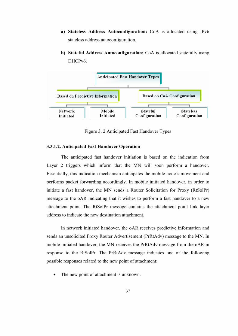
37

a) Stateless Address Autoconfiguration: CoA is allocated using IPv6

stateless address autoconfiguration.

b) Stateful Address Autoconfiguration: CoA is allocated statefully using

DHCPv6.

Figure 3. 2 Anticipated Fast Handover Types

3.3.1.2. Anticipated Fast Handover Operation

The anticipated fast handover initiation is based on the indication from

Layer 2 triggers which inform that the MN will soon perform a handover.

Essentially, this indication mechanism anticipates the mobile node’s movement and

performs packet forwarding accordingly. In mobile initiated handover, in order to

initiate a fast handover, the MN sends a Router Solicitation for Proxy (RtSolPr)

message to the oAR indicating that it wishes to perform a fast handover to a new

attachment point. The RtSolPr message contains the attachment point link layer

address to indicate the new destination attachment.

In network initiated handover, the oAR receives predictive information and

sends an unsolicited Proxy Router Advertisement (PrRtAdv) message to the MN. In

mobile initiated handover, the MN receives the PrRtAdv message from the oAR in

response to the RtSolPr. The PrRtAdv message indicates one of the following

possible responses related to the new point of attachment:

• The new point of attachment is unknown.

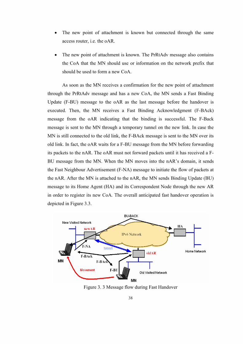
38

• The new point of attachment is known but connected through the same

access router, i.e. the oAR.

• The new point of attachment is known. The PrRtAdv message also contains

the CoA that the MN should use or information on the network prefix that

should be used to form a new CoA.

As soon as the MN receives a confirmation for the new point of attachment

through the PrRtAdv message and has a new CoA, the MN sends a Fast Binding

Update (F-BU) message to the oAR as the last message before the handover is

executed. Then, the MN receives a Fast Binding Acknowledgment (F-BAck)

message from the oAR indicating that the binding is successful. The F-Back

message is sent to the MN through a temporary tunnel on the new link. In case the

MN is still connected to the old link, the F-BAck message is sent to the MN over its

old link. In fact, the oAR waits for a F-BU message from the MN before forwarding

its packets to the nAR. The oAR must not forward packets until it has received a F-

BU message from the MN. When the MN moves into the nAR’s domain, it sends

the Fast Neighbour Advertisement (F-NA) message to initiate the flow of packets at

the nAR. After the MN is attached to the nAR, the MN sends Binding Update (BU)

message to its Home Agent (HA) and its Correspondent Node through the new AR

in order to register its new CoA. The overall anticipated fast handover operation is

depicted in Figure 3.3.

Figure 3. 3 Message flow during Fast Handover

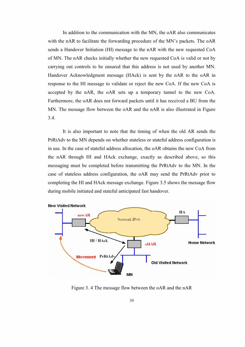
39

In addition to the communication with the MN, the oAR also communicates

with the nAR to facilitate the forwarding procedure of the MN’s packets. The oAR

sends a Handover Initiation (HI) message to the nAR with the new requested CoA

of MN. The nAR checks initially whether the new requested CoA is valid or not by

carrying out controls to be ensured that this address is not used by another MN.

Handover Acknowledgment message (HAck) is sent by the nAR to the oAR in

response to the HI message to validate or reject the new CoA. If the new CoA is

accepted by the nAR, the oAR sets up a temporary tunnel to the new CoA.

Furthermore, the oAR does not forward packets until it has received a BU from the

MN. The message flow between the oAR and the nAR is also illustrated in Figure

3.4.

It is also important to note that the timing of when the old AR sends the

PrRtAdv to the MN depends on whether stateless or stateful address configuration is

in use. In the case of stateful address allocation, the oAR obtains the new CoA from

the nAR through HI and HAck exchange, exactly as described above, so this

messaging must be completed before transmitting the PrRtAdv to the MN. In the

case of stateless address configuration, the oAR may send the PrRtAdv prior to

completing the HI and HAck message exchange. Figure 3.5 shows the message flow

during mobile initiated and stateful anticipated fast handover.

Figure 3. 4 The message flow between the oAR and the nAR

40

Figure 3. 5 Message flow during Mobile Initiated and Stateful Fast Handover

3.3.2. Tunnel Based Fast Handover

The Tunnel Based Fast Handover is similar to the Anticipated Fast

Handover. The main difference between the Tunnel Based Fast Handover and the

Anticipated Fast Handover is that in Tunnel Based Fast Handover the MN delays

the new CoA establishment when it moves to a nAR and only performs Layer 2

handover and continues to use its old CoA in the new subnet. The Layer 3 handover

is carried out, when the MN has enough time to complete the Layer 3 handover.

In this mechanism, in order to deliver packets to the MN and send packets

from the MN to the Correspondent Node (CN), bidirectional edge tunnels are set up

41

between the oAR and the nAR. When the packets destined to the MN reach the old

subnet, the oAR tunnels the corresponding packets to the nAR. When the MN sends

packets to the CN, the outgoing packets of the MN take the reverse path in the

bidirectional edge tunnel from the nAR to the oAR which forwards them to the CN.

The Tunnel Based Fast Handover depends on the use of bidirectional edge tunnels

and is sometimes referred to Bidirectional Edge Tunnel Handover (BETH).

Furthermore, if the MN moves quite fast, the bidirectional tunnel is extended to a

third AR, i.e. handover to third (HTT), as shown in Figure 3.6. In this case, the nAR

signals the anchor Access Router (aAR) to move the wireless link end of the tunnel

to itself, i.e. the nAR. Therefore, the MN moves with the help of establishment of a

series of tunnels between the ARs, with one end of the tunnel remaining fixed to the

aAR and the other end of the tunnel changing to the current access router.

Figure 3. 6 Handover to third scenario for Tunnel Based Handover

42

3.3.3. Evaluation of Fast Handover for Mobile IPv6

Fast Handover for Mobile IPv6 protocol aims to improve the handover

performance of the standard Mobile IPv6 protocol by minimizing the latency for

establishing new communication paths from the MN to the nAR without any packet

loss. However, some packets can still be lost if there is a random and rapid

movement of the MN from one AR to another without letting any handover process

to be completed. In the following section, the Simultaneous Bindings for Mobile

IPv6 which is one of the proposed protocols to solve such a problem will be

described.

3.4. Simultaneous Bindings for Mobile IPv6

Fast Handover for Mobile IPv6 protocol (Fast MIPv6) describe

enhancements with the goal to minimize service disruption during handover. The

Simultaneous Bindings for Mobile IPv6 protocol [6] extends these enhancements

with a simultaneous binding function to minimize packet loss at the MN. However,

it is difficult to estimate the correct time to start forwarding traffic between the oAR

and the nAR, which has an impact on how smooth the handoff will be. Packet loss

will occur if this forward service is performed too late or too early with respect to

the time in which the MN detaches from the oAR and attaches to the nAR. The

simultaneous bindings function solves this problem by allowing traffic for the MN

to be bicasted or N-casted for a short period to its current location and to one or

more locations where the MN is expected to move to shortly.

The goal for the simultaneous bindings function is to reduce packet loss at

the Mobile Node and to remove the timing ambiguity regarding when to start

sending traffic for the Mobile Node to its new point of attachment following a Fast

Handover. Another important goal for this function is to save the MN periods of

service disruption in case of so-called ping-pong movement, i.e. when a MN moves

back and forth between two Access Routers.

Moreover, the simultaneous binding function is an extension to the Fast

Binding Update message used in Fast MIPv6. The only difference between the Fast

43

Binding Update message used in Fast MIPv6 and the Fast Binding Update message

used in Simultaneous Bindings for MIPv6 is the Simultaneous Bindings Flag. It is

important to note that F-BU with simultaneous binding message sent from the MN

to the MAP also includes the life time field to identify the life time of simultaneous

bindings. When this life time expires, the forwarding procedure is terminated. There

are two types of simultaneous binding functions, namely bicasting of and N-casting

simultaneous binding function:

• Bicasting Simultaneous Binding Function: Bicasting function is used

when the MN is receiving loss sensitive traffic. By using this function, each

packet flow is duplicated towards the MN’s current location and the

potential or future location of the MN, as illustrated in Figure 3.7.

Figure 3. 7 Bicasting Simultaneous Binding Function

• N-casting Simultaneous Binding Function: N-casting function is quite

similar to Bicasting function. The major difference is that the packet flows

are duplicated towards three or more potential future locations for the MN,

as illustrated in Figure 3.8. There is a phenomenon called ping-pong

movement that might occur when the MN is close to two or more Access

Routers (ARs) and moves back and forth between them. Sending the same

traffic to all the potential ARs might solve ping-pong movement problem.

44

Figure 3. 8 N-casting Simultaneous Binding Function

3.4.1. Evaluation of Simultaneous Bindings for Mobile IPv6

Simultaneous Bindings for Mobile IPv6 protocol provides a good solution to

the ping-pong movement, i.e. when the MN moves back and forth between two

Access Routers, by bicasting or N-casting the traffic for a short period. Another big

advantage is that this protocol removes the timing problem in Anticipated Fast

Handover, i.e. to determine the time when to start forward packets to the nAR.

Thus, this enhanced mechanism, i.e. simultaneous binding function, provides the

MN with uninterrupted connectivity.

A drawback of Simultaneous Bindings for Mobile IPv6 protocol is that this

protocol might cause too much overhead in the network. The fact that traffic is

bicasted or n-casted might create network congestions and network might become

overloaded. Therefore, bicasting or N-casting might not be a scalable solution in a

network with a lot of fast moving MNs and many neighbouring Access Routers.

This may result in too much traffic for the network to handle. As a result, it is

significant to find the suitable mixing of what traffic should be bicasted and what

shouldn’t.

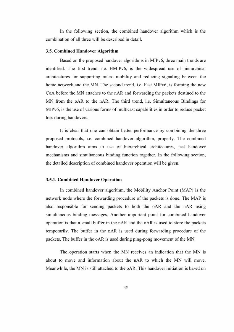
45

In the following section, the combined handover algorithm which is the

combination of all three will be described in detail.

3.5. Combined Handover Algorithm

Based on the proposed handover algorithms in MIPv6, three main trends are

identified. The first trend, i.e. HMIPv6, is the widespread use of hierarchical

architectures for supporting micro mobility and reducing signaling between the

home network and the MN. The second trend, i.e. Fast MIPv6, is forming the new

CoA before the MN attaches to the nAR and forwarding the packets destined to the

MN from the oAR to the nAR. The third trend, i.e. Simultaneous Bindings for

MIPv6, is the use of various forms of multicast capabilities in order to reduce packet

loss during handovers.

It is clear that one can obtain better performance by combining the three

proposed protocols, i.e. combined handover algorithm, properly. The combined

handover algorithm aims to use of hierarchical architectures, fast handover

mechanisms and simultaneous binding function together. In the following section,

the detailed description of combined handover operation will be given.

3.5.1. Combined Handover Operation

In combined handover algorithm, the Mobility Anchor Point (MAP) is the

network node where the forwarding procedure of the packets is done. The MAP is

also responsible for sending packets to both the oAR and the nAR using

simultaneous binding messages. Another important point for combined handover

operation is that a small buffer in the nAR and the oAR is used to store the packets

temporarily. The buffer in the nAR is used during forwarding procedure of the

packets. The buffer in the oAR is used during ping-pong movement of the MN.

The operation starts when the MN receives an indication that the MN is

about to move and information about the nAR to which the MN will move.

Meanwhile, the MN is still attached to the oAR. This handover initiation is based on

46

the indication from Layer 2 triggers which inform that the MN will soon perform a

handover.

In mobile initiated handover, the MN receives the predictive information, i.e.

Layer 2 trigger, and then it sends a Router Solicitation for Proxy (RtSolPr) message

to the oAR indicating that it wishes to perform a fast handover to a new attachment

point. The RtSolPr message contains the attachment point link layer address to

indicate the new destination attachment.

In network initiated handover, the oAR receives predictive information and

sends an unsolicited Proxy Router Advertisement (PrRtAdv) message to the MN

without receiving RtSolPr message from the MN.

If the oAR knows the new point of attachment and has information about the

network prefix that should be used to form a new CoA, it sends a confirmation for

the new point of attachment through the PrRtAdv message to the MN. When the

MN receives the PrRtAdv message from the oAR, it forms the new CoA using

stateless address autoconfiguration.

Furthermore, the oAR has to inform the MAP about the possibility of the

handover to control newly formed CoA in the nAR. To inform the MAP, the oAR

sends Handover Initiation (HI) message to the corresponding MAP including old

CoA, new CoA and the address of the nAR. It is important to note that the oAR

should know the address of the corresponding MAP which the MN is

communicating with. This address is provided in the RtSolPr message.

When the MAP receives HI, it sends it to the nAR including the newly

formed CoA. The new AR checks whether this address is currently in used or not.

With the result of the address checking, the new Access Router sends the Handover

Acknowledgment (HACK) message to the MAP, indicating how to forward the

packets. If the address checking process is successful, the forwarding is made to the

new CoA. Otherwise, the MAP establishes a tunnel to the nAR, and the nAR

forwards the packets to the actual link. In this case, the MN still uses the old CoA.

47

To start the process of forwarding, the MN sends a Fast Binding Update (F-

BU) message with simultaneous binding to the MAP so as to bind the regional CoA

with the new CoA. After receiving the F-BU with simultaneous binding, the MAP

sends a Fast Binding Acknowledgment (F-BAck) message to the oAR and nAR and

starts to forward the packets destined to the MN, using bicasting. It is not necessary

to know the precise movement of the MN, since the MAP sends the packets to both

the nAR and the oAR. Therefore, the packet losses result from the synchronization

problem is avoided. Another significant point is that the F-BU with simultaneous

binding message sent from the MN to the MAP includes the life time field to

identify the life time of simultaneous bindings. When this life time expires, the

forwarding procedure is terminated.

When forwarded packets reach to the nAR, the MN might not arrive to the

nAR yet. In order not to lose any packet, it is necessary to store forwarded packets

in a buffer in the nAR. When the MN arrives to the nAR, it sends a Fast Neighbour

Advertisement (F-NA) message, advertising its arrival to the nAR. After receiving

F-NA message, the nAR starts to send the packets stored in its buffer. In case of

ping-pong movement, the packets stored in the buffer of the oAR is used for lossless

communication. If the MN comes back to the old subnet and sends F-BU message

to the oAR, the oAR can deliver the buffered packets to the MN.

In case of stateful address configuration, the nAR sends the valid new CoA

with the HACK message to the MAP. The MAP then sends the PrRtAdv message to

the MN providing the new CoA.

After the MN is attached to the nAR, the MN checks the MAP option in the

PrRtAdv message received by the nAR so as to determine whether it is in a new

MAP domain or not. In addition, the MN needs to know whether the new CoA sent

with the F-BU message is still valid or not. This information is provided by the F-

Back message. If the MN moves to a new MAP domain, the new MAP also sends

Binding Update message to the home agent (HA) and the correspondent node (CN)

to bind the regional CoA with the Home Address. The operation of the combined

handover algorithm is illustrated in Figure 3.9.

48

Figure 3. 9 Message flow of combined handover algorithm during handover

3.5.2. Evaluation of Combined Handover Algorithm

The combined handover algorithm reduces the packet loss to a minimum by

combining each improvement of three protocols efficiently. In combined handover

algorithm, the hierarchical architecture decreases the handover latency by reducing

unnecessary control signals during micro mobility. Furthermore, the fast handover

algorithm with simultaneous binding function minimizes packet losses by forming

the new CoA before the MN attaches to the nAR and forwarding the packets to both

the oAR and nAR for a short period of time. The fast handover algorithm with

simultaneous binding function removes the timing ambiguity, i.e. to determine the

time when to start forwarding packets to the nAR. Although the forwarding

49

procedure in combined handover protocol solves the synchronization problem and

provides lossless communication, it might also cause congestion in the network.

In combined handover algorithm, the MAP, instead of the Access Router

(AR) as in fast handover algorithm case, forwards the packets to both the oAR and

the nAR. The forwarding path is optimized, because the MAP is in a high level in

the hierarchy compared to the AR. Therefore, unnecessary packet transfer between

the MAP and the ARs is prevented to improve the bandwidth efficiency. In addition,

the bottleneck problem of the hierarchical architecture, i.e. the fact that all the

communications within the MAP domain pass across the MAP, remains in

combined handover algorithm.

In this algorithm, the buffer in both the oAR and the nAR is used for not

losing any packets during forwarding procedure and ping-pong movement of the

MN. The size of these buffers should be selected properly in order to satisfy real

time application requirements. If the handover latency is greater than the time that

the corresponding buffer can store, the forwarded packets are lost. If a large buffer

is selected to be able to store packets in a great amount of time, it becomes useless

in real time applications like Voice over IP. Making the buffer larger is not a

feasible solution for delay sensitive traffic, i.e. real time applications, since the total

delay in stored packets may become intolerable. For instance, human factors studies

have shown that the maximum tolerable delay for interactive conversations is

approximately 200 ms [40]. Thus, the maximum permitted end to end delay of real

time applications restricts the amount of time that a buffer can store. In addition, the

scalability problems due to the necessity of buffers in the Access Routers may occur

in combined handover protocol.

In this algorithm, the movement detection problem of the MN is solved by

using Layer 2 triggers advertising that the MN arrives the nAR. Thus, the

dependency on the router advertisement messages to detect movement of the MN is

avoided. However, how to handle Layer 2 triggers properly is another research issue

which should be solved by hardware manufacturers.

50

In conclusion, the combined handover algorithm introduces a more complete

and elegant solution to mobility management compared to the proposed protocols.

However, the scalability problems and the possible bottleneck problem of this

protocol should also be taken into account in order to provide efficient handover

mechanism to the mobile users.

51

CHAPTER 4

MODELING OF NETWORK TRAFFIC AND USER MOBILITY

Simulating how the global Internet behaves is an immensely complex issue

because of the network’s great heterogeneity and rapid change. The heterogeneity of

the Internet ranges from different characteristics of the links that carry the network’s

traffic to the protocols that interoperate over these links and to the “mix” of different

applications used at a site [41]. Due to the network’s complexity and heterogeneity,

simulation and modeling plays a vital role in attempting to evaluate the performance

of the proposed algorithms and architectures. It is also important to note that

simulations are complementary to analysis by allowing understanding of

complicated scenarios that would be either difficult or impossible to analyze.

The future mobile communication networks, e.g. 3G or 4G wireless

networks, target to support global roaming and integrated services such as the voice,

data and multimedia with mobile computing devices over the wireless

infrastructures. Modeling of traffic generation and user mobility for such networks

is challenging and important to analyze the possible effect of proposed changes with

appropriate accuracy. In the following sections, the details of modeling of network

traffic and user mobility performed within this thesis will be discussed.

4.1. Modeling of Network Traffic

Data traffic is the main component of computer communication systems, and

traffic models are of crucial importance for assessing their performance [42]. In

52

practice, stochastic models of network traffic are relevant to communication

network analysis and teletraffic engineering and they are widely used in predicting

the performance of the proposed methods.

Due to analytical tractability, many researchers used the traditional network

modeling, i.e. Poisson or Markovian modeling, to model the network traffic in the

past for many years. Traditional network models typically focus on very limited

range of time scales and are thus short range dependent in nature. They also predict

that longer term correlations should rapidly die out, and consequently that traffic

observed on large time scales should appear quite smooth. Nevertheless, a wide

body of empirical data argues strongly that these correlations remain nonnegligible

over a large range of time scales. Statistical analysis of high resolution traffic

measurements from a wide range of networks, e.g. Local Area Networks (LANs),

Wide Area Networks (WANs), World Wide Web (WWW) transfers and VBR video

over ATM, show that number of packets that pass through the given link per unit

time exhibit self similar or fractal behaviour ([7], [43], [44] and [45] to name a few).

Self similar behaviour which underlies long range dependency means that a segment

of the traffic rate process measured at some scale looks like an appropriately scaled

version of the traffic rate process measured over a different time scale.

The pictorial proof and mathematical background of the self similar nature

of the packet traffic is first presented in [7], as illustrated in Figure 4.1. The reason

for the significance of this work is that up to this point, network traffic was modeled

as a Poisson process and all analysis of networks were based on that assumption.

Furthermore, it has been shown in the literature ([43], [46] and [47]) that self

similar or long range dependent (LRD) network traffic can be generated by

multiplexing several sources of Pareto distributed ON and OFF periods. Pareto

distribution has the following probability density function:

f (x) = α βα

x α +1 , where β≥x and 21 ≤≤ α for finite variance and mean.

53

Figure 4. 1 Pictorial proof of self similarity: Ethernet traffic on 5 different scales

54

In a context of a packet switched network, the ON periods correspond to

packet bursts, i.e. packets transmitted back to back or separated only by a relatively

small preamble, and OFF periods are the periods of silence between packet bursts.

Multiple sources contributing to resulting synthetic traffic trace might be thought of

as individual flows, i.e. connections. It is reasonable to assume that packet sizes

within a connection remain constant. Different connections, however, will have

packets of different sizes.

During research in the internet, the utility* that generates self similar traffic

by aggregating multiple sources of Pareto distributed ON and OFF periods is found.

In this utility, every source generates packets of only one size and Pareto

distribution of burst sizes is achieved by using Pareto distribution for the number of

packets in a burst. Inter burst gaps are also Pareto distributed. In this thesis, this

utility is used for generating self similar traffic. To generate self similar traffic, the

sources generating packets of 128 Bytes are used and the shape parameter of Pareto

distribution is selected as 1.4 and 1.2 for the ON periods and the OFF periods,

respectively. The choice of the shape parameter for the ON periods is made

according to the measurements on actual Ethernet traffic performed by Leland et al.

[7]. They reported that the measured Hurst parameter (H) is 0.8 for moderate

network load. In [43], the relationship between the Hurst parameter and the shape

parameter (α) is given as follows:

H = (3 - α) / 2.

Therefore, the Hurst parameter of 0.8 results in shape parameter of 1.4.

4.2. Modeling of User Mobility

The rapid growth of mobile communication services, together with the

scarcity of radio spectrum has lead to reducing the cell size in cellular systems.

Smaller and denser cells provide higher aggregate bandwidth and can locate a

mobile device more accurately. On the other hand, smaller cell size entails a higher

handover rate and more frequent handovers per call [48]. Hence, the study of *http://wwwcsif.cs.ucdavis.edu/~kramer/code/trf_gen1.html

55

handover related aspects has become a fundamental issue in which a good

knowledge of user mobility modeling and characterization of mobility patterns is of

paramount importance for research and design issues of handover algorithms.

The movement pattern of the mobile users plays an important role in

performance analysis of mobile and wireless networks. For example, in cellular

networks, a user's mobility behavior directly affects the signaling traffic needed for

handover management [49]. With the increasing number of mobile users and the

decreasing cell size in wireless communication networks, modeling the user’s

mobility will have even more influence on the performance issues of handover

algorithms. The modeling of the mobile user's movement is thus an essential

building block in analytical and simulation based studies of handover mechanisms.

Furthermore, the choice of the mobility model has a significant effect on the

obtained results. If the model is unrealistic, invalid conclusions may be drawn.

A literature survey shows that there exist several mobility models that find

application in different kinds of simulations and analytical studies of wireless

networks. Analytical mobility models are generally based on rather simple

assumptions regarding the movement behavior of the users, but these models enable

to evaluate the performance of proposed handover algorithms. The user’s mobility

can be characterized by the amount of time that the mobile user stays in that cell, i.e.

the cell residence time [50]. Therefore, an appropriate probability distribution that

accurately describes the cell residence time is of great significance to be

investigated.

A considerable amount of research effort ([51], [52], [53], [54] and

references therein) has been devoted to derive the distribution of the cell residence

time. In addition, a great deal of papers dealing with wireless and mobile

communications have used these studies. For the sake of convenience and

tractability, most previous traffic analysis made the assumption that the cell

residence time is distributed exponentially ([55], [56], [57], [58] and [59] to name a

few). However, some experiments with operational systems and field data revealed

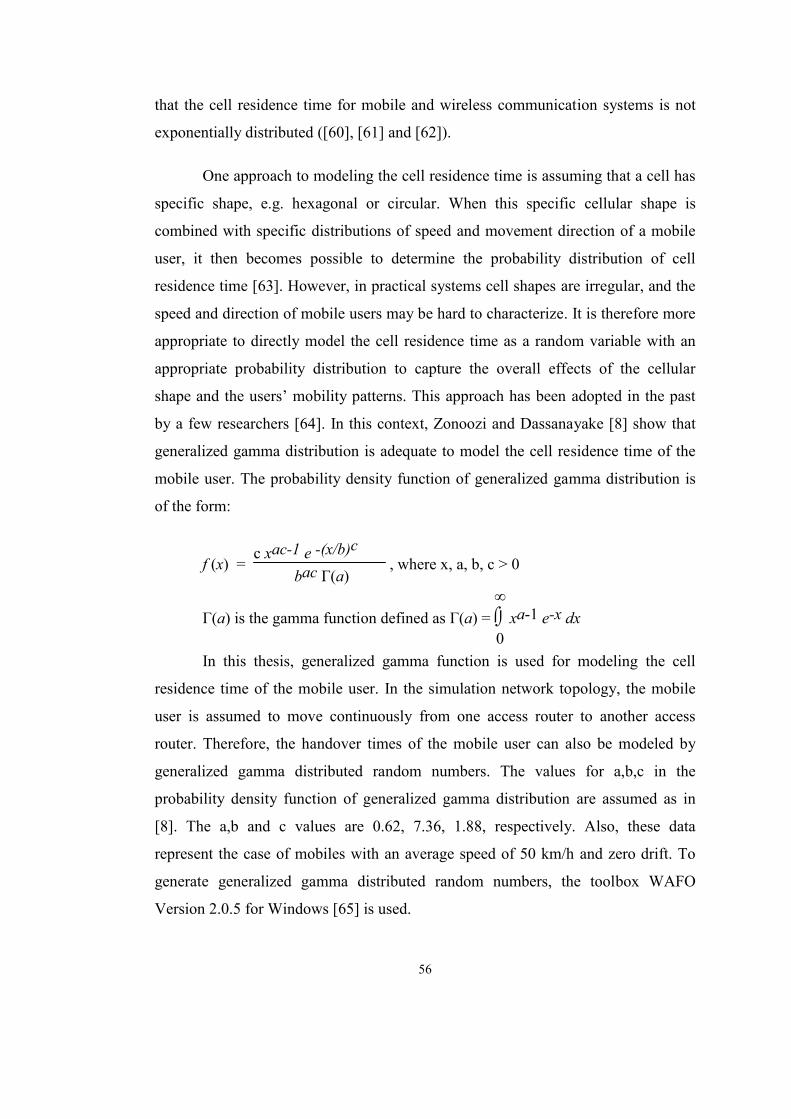
56

that the cell residence time for mobile and wireless communication systems is not

exponentially distributed ([60], [61] and [62]).

One approach to modeling the cell residence time is assuming that a cell has

specific shape, e.g. hexagonal or circular. When this specific cellular shape is

combined with specific distributions of speed and movement direction of a mobile

user, it then becomes possible to determine the probability distribution of cell

residence time [63]. However, in practical systems cell shapes are irregular, and the

speed and direction of mobile users may be hard to characterize. It is therefore more

appropriate to directly model the cell residence time as a random variable with an

appropriate probability distribution to capture the overall effects of the cellular

shape and the users’ mobility patterns. This approach has been adopted in the past

by a few researchers [64]. In this context, Zonoozi and Dassanayake [8] show that

generalized gamma distribution is adequate to model the cell residence time of the

mobile user. The probability density function of generalized gamma distribution is

of the form:

f (x) = c xac-1 e -(x/b)c

bac Γ(a) , where x, a, b, c > 0

Γ(a) is the gamma function defined as Γ(a) = ⌡⌠0

∞ xa-1 e-x dx

In this thesis, generalized gamma function is used for modeling the cell

residence time of the mobile user. In the simulation network topology, the mobile

user is assumed to move continuously from one access router to another access

router. Therefore, the handover times of the mobile user can also be modeled by

generalized gamma distributed random numbers. The values for a,b,c in the

probability density function of generalized gamma distribution are assumed as in

[8]. The a,b and c values are 0.62, 7.36, 1.88, respectively. Also, these data

represent the case of mobiles with an average speed of 50 km/h and zero drift. To

generate generalized gamma distributed random numbers, the toolbox WAFO

Version 2.0.5 for Windows [65] is used.

57

CHAPTER 5

SIMULATION EXPERIMENTS

In this chapter, the algorithms proposed in the literature and the combined

handover method are evaluated and compared through simulations. Moreover, a

simulation model suitable for evaluation of the proposed handover algorithms under

some certain scenarios will be described. The network topology used in simulation

is shown in Figure 5.1. In this simulated network architecture, the user mobility, the

network traffic, wired and wireless links are modeled through stochastic processes.

Firstly, the network traffic is modeled by both traditional framework modeling

(termed Poisson modeling) and self similar traffic modeling [7]. Secondly, the user

mobility is modeled by assuming that cell residence time of the mobile user exhibits

generalized gamma distribution [8]. Thirdly, the wired links in simulation network

architecture are modeled from real traces taken on the Internet between April and

August of 2003. The programs used in simulations are as follows:

• Rhapsody version 4.0.1: Rhapsody is used for implementing and analyzing

the proposed handover algorithms by using C++ Programming Language.

Rhapsody is a Unified Modeling Language (UML) based tool that has the

ability of allowing software developers to specify, visualize and construct

the artifacts of a system before committing it to code and also promotes the

building of reusable components. These features of Rhapsody help us to

code the handover algorithms efficiently.

58

• MATLAB version 6.5: MATLAB is used for the performance evaluation of

the handover algorithms. The performance graphics are also plotted by

MATLAB and the user mobility is modeled by MATLAB in conjunction

with the toolbox WAFO Version 2.0.5 for Windows [65].

• Table Curve 2D version 4.0: Table Curve 2D is used in curve fitting for the

round trip time of the wired links in simulated network topology.

• Visual Traceroute, Neo-Trace, Ping: These applications are used for

collecting data from the Internet and tracing the measurement packets

visually.

Figure 5. 1 Simulation Network Topology

In the following section, the measurement methods for modeling the link

delay will be discussed.

59

5.1. Measurement Methods for Modeling the Link Delay

Packet probing is an important Internet measurement technique, supporting

the investigation of packet delay. Current packet probing techniques use Internet

Protocols such as the Internet Control Message Protocol (ICMP), the User Datagram

Protocol (UDP) and the Transmission Control Protocol (TCP). The examples of

current measurement techniques which use these protocols are ping, traceroute and

the IP Performance Metrics (IPPM) group’s One-way Delay Protocol (OWDP) [66].

5.1.1. Ping

Ping is one of the most useful network debugging tools which is

implemented by using the Internet Control Message Protocol (ICMP) detailed in

[67]. The ping utility is essentially a system administrator's tool that is used to see if

a computer is operating and also to see if the network connections are intact. By

using the ping application, round trip time (RTT) is calculated as the difference

between the time the echo request is sent and the time a matching response is

received.

5.1.2. Traceroute

Traceroute is a network debugging utility that attempts to trace the route of a

packet takes through the network. In a typical traceroute session, a group of packets

with time to live (TTL) value initially set to one are sent. Reminding that TTL is an

IP header field that is designed to prevent packets from running in loops. Every

router that handles a packet subtracts one from the packet's TTL. If the TTL reaches

zero, the packet has expired and is discarded. Moreover, traceroute depends on the

common router practice of sending an ICMP Time Exceeded message back to the

sender when this fact occurs. By using small TTL values which quickly expire,

traceroute causes routers along a packet's normal delivery path to generate these

ICMP messages which identify the router. For example, A TTL value of one should

produce a message from the first router, a TTL value of two generates a message

from the second router and a TTL value of three generates a message from the third

and etc. [68].

60

5.1.3. One Way Delay Protocol

The IP Performance Metrics (IPPM) group has published several studies that

define frameworks for measuring the performance of IP networks ([69] and [70]).

The IPPM group is well advanced in the engineering of a One-way Delay

Measurement Protocol (OWDP) [71] that will build on a framework designed in

[72]. The OWDP specification provides a mechanism for measuring packet delay

with UDP packet probes. Furthermore, the specification describes a mechanism for

controlling a measurement session between two hosts with a TCP connection, for

negotiating the UDP port numbers involved in the delay measurement.

5.2. Measurement Method Used in the Thesis

In this thesis, the ping method is used for the investigation of the packet

delay in the wired links. The measurements are done in different days and hours

between April and August of 2003. In the simulated network topology, the wired

links need to be modeled are the links between CN and HA or MAP and the links

between HA and MAPs or MAPs and ARs. The link delay between CN and HA or

MAP might be assumed as a typical delay in Wide Area Network (WAN) and the

link delay between HA and MAPs or MAPs and ARs might be assumed as a typical

delay in Metropolitan Area Network (MAN) [73]. The nodes in measurement

architecture are selected according to these criteria. The measurement architecture

for modeling the wired link delays is illustrated in Figure 5.2. The ping application

is called from the main node to other nodes given in Table 5.1. Although, one way

delay for a path between two nodes is not equal to each other, we assumed that the

half of the measured RTT for a path can be used as a one way delay.

Table 5. 1 Node Locations

Node Number Node Location IP Address 1 Aselsan Inc.,Ankara 10.1.6.170 2 METU, Ankara 144.122.199.13 3 Ankara University 80.251.40.19 4 İstanbul University 194.27.128.199 5 MIT,Boston,USA 18.181.0.31

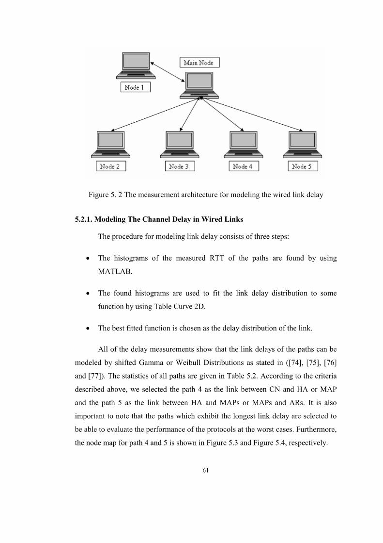
61

Figure 5. 2 The measurement architecture for modeling the wired link delay

5.2.1. Modeling The Channel Delay in Wired Links

The procedure for modeling link delay consists of three steps:

• The histograms of the measured RTT of the paths are found by using

MATLAB.

• The found histograms are used to fit the link delay distribution to some

function by using Table Curve 2D.

• The best fitted function is chosen as the delay distribution of the link.

All of the delay measurements show that the link delays of the paths can be

modeled by shifted Gamma or Weibull Distributions as stated in ([74], [75], [76]

and [77]). The statistics of all paths are given in Table 5.2. According to the criteria

described above, we selected the path 4 as the link between CN and HA or MAP

and the path 5 as the link between HA and MAPs or MAPs and ARs. It is also

important to note that the paths which exhibit the longest link delay are selected to

be able to evaluate the performance of the protocols at the worst cases. Furthermore,

the node map for path 4 and 5 is shown in Figure 5.3 and Figure 5.4, respectively.

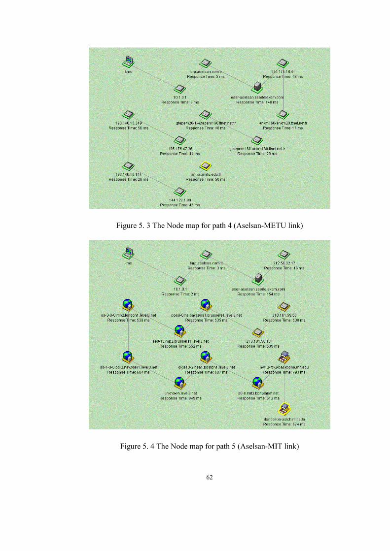
62

Figure 5. 3 The Node map for path 4 (Aselsan-METU link)

Figure 5. 4 The Node map for path 5 (Aselsan-MIT link)

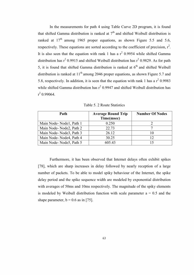
63

In the measurements for path 4 using Table Curve 2D program, it is found

that shifted Gamma distribution is ranked at 7th and shifted Weibull distribution is

ranked at 17th among 1965 proper equations, as shown Figure 5.5 and 5.6,

respectively. These equations are sorted according to the coefficient of precision, r2.

It is also seen that the equation with rank 1 has a r2 0.9954 while shifted Gamma

distribution has r2 0.9915 and shifted Weibull distribution has r2 0.9829. As for path

5, it is found that shifted Gamma distribution is ranked at 6th and shifted Weibull

distribution is ranked at 11th among 2046 proper equations, as shown Figure 5.7 and

5.8, respectively. In addition, it is seen that the equation with rank 1 has a r2 0.9983

while shifted Gamma distribution has r2 0.9947 and shifted Weibull distribution has

r2 0.99064.

Table 5. 2 Route Statistics

Path Average Round Trip Time(msec)

Number Of Nodes

Main Node- Node1, Path 1 0.250 2 Main Node- Node2, Path 2 22.73 7 Main Node- Node3, Path 3 26.12 10 Main Node- Node4, Path 4 30.25 12 Main Node- Node5, Path 5 605.43 15

Furthermore, it has been observed that Internet delays often exhibit spikes

[78], which are sharp increases in delay followed by nearly reception of a large

number of packets. To be able to model spiky behaviour of the Internet, the spike

delay period and the spike sequence width are modeled by exponential distribution

with averages of 50ms and 10ms respectively. The magnitude of the spiky elements

is modeled by Weibull distribution function with scale parameter a = 0.5 and the

shape parameter, b = 0.6 as in [75].

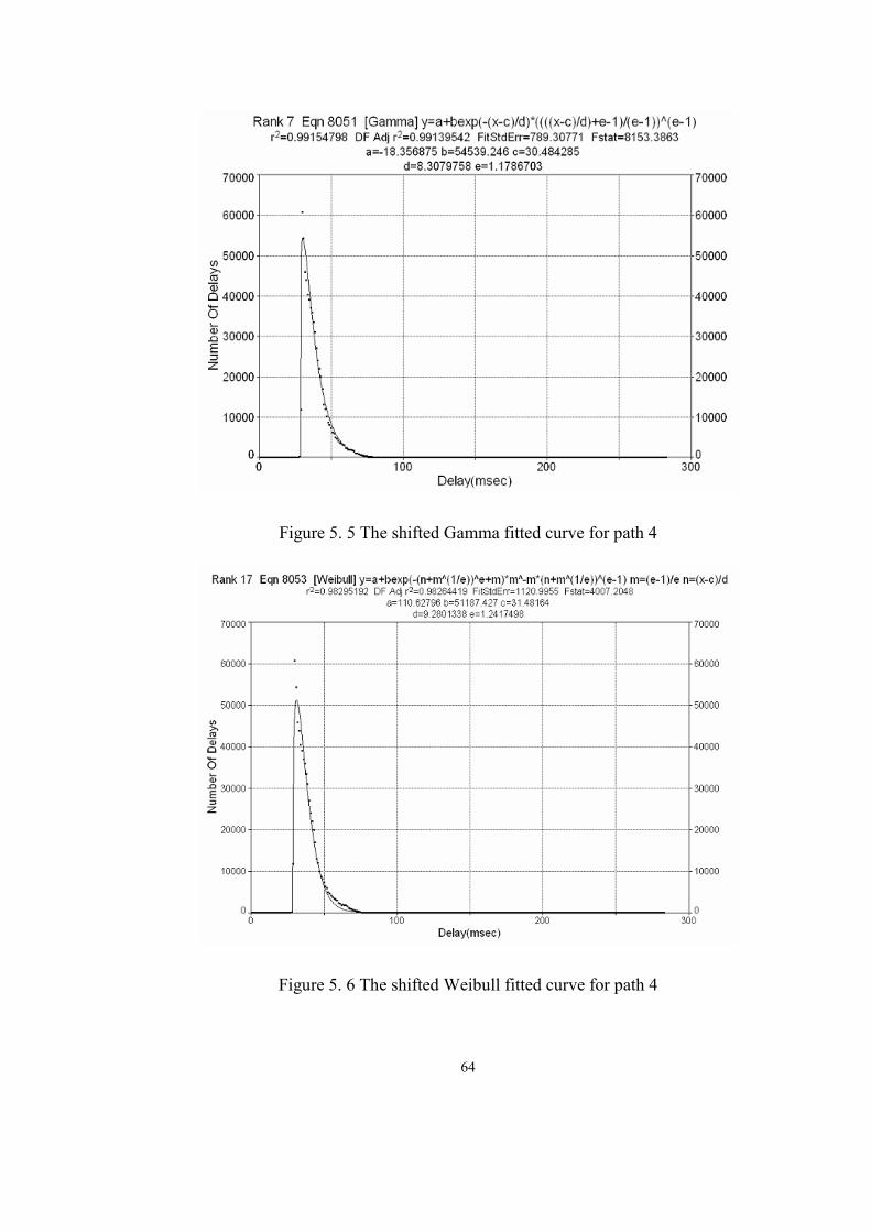
64

Figure 5. 5 The shifted Gamma fitted curve for path 4

Figure 5. 6 The shifted Weibull fitted curve for path 4

65

Figure 5. 7 The shifted Gamma fitted curve for path 5

Figure 5. 8 The shifted Weibull fitted curve for path 5

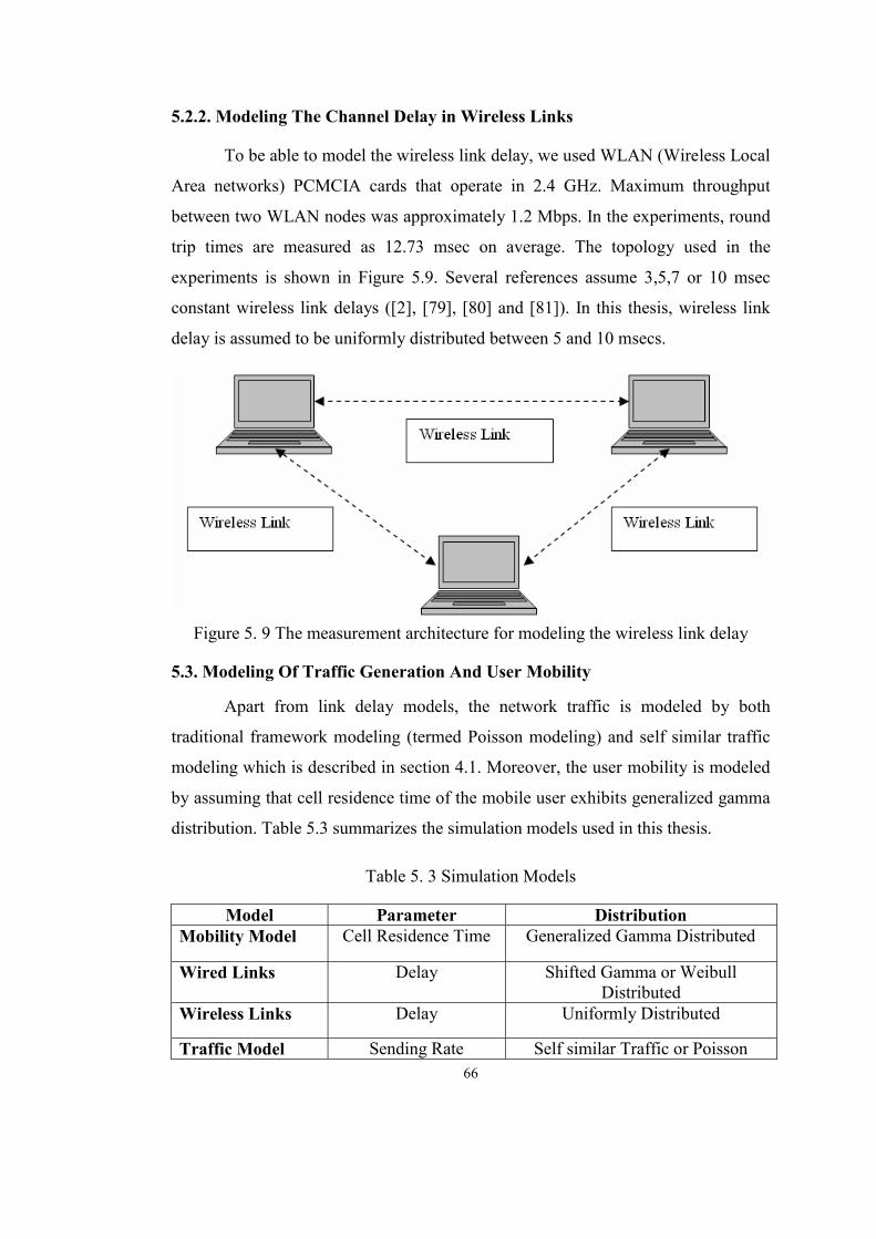
66

5.2.2. Modeling The Channel Delay in Wireless Links

To be able to model the wireless link delay, we used WLAN (Wireless Local

Area networks) PCMCIA cards that operate in 2.4 GHz. Maximum throughput

between two WLAN nodes was approximately 1.2 Mbps. In the experiments, round

trip times are measured as 12.73 msec on average. The topology used in the

experiments is shown in Figure 5.9. Several references assume 3,5,7 or 10 msec

constant wireless link delays ([2], [79], [80] and [81]). In this thesis, wireless link

delay is assumed to be uniformly distributed between 5 and 10 msecs.

Figure 5. 9 The measurement architecture for modeling the wireless link delay

5.3. Modeling Of Traffic Generation And User Mobility

Apart from link delay models, the network traffic is modeled by both

traditional framework modeling (termed Poisson modeling) and self similar traffic

modeling which is described in section 4.1. Moreover, the user mobility is modeled

by assuming that cell residence time of the mobile user exhibits generalized gamma

distribution. Table 5.3 summarizes the simulation models used in this thesis.

Table 5. 3 Simulation Models

Model Parameter Distribution Mobility Model Cell Residence Time Generalized Gamma Distributed

Wired Links Delay Shifted Gamma or Weibull Distributed

Wireless Links Delay Uniformly Distributed

Traffic Model Sending Rate Self similar Traffic or Poisson

67

5.4. Performance Results

Simulation is at best an approximation to the real world. The main focus of

this thesis is to investigate and analyze the packet losses due to handover. For the

sake of simplicity in the simulation, the other reasons for packet loss such as

congestion, link characteristics are not included.

In simulation experiments of the proposed handover algorithms, average

packet loss percentages vs. handover rate of the mobile user are analyzed. As

mentioned before, the network traffic is both modeled by both traditional framework

modeling (termed Poisson modeling) and self similar traffic modeling. In the

simulations, Poisson arrival rates are considered to be 1, 0.1, 0.05 packets/sec,

respectively. Also, the advertisement period, i.e. beacon period, is assumed as 50

msecs and the time the mobile user receives Layer 2 trigger before handover is

supposed to be uniformly distributed between 50 and 100 msecs. Furthermore, a

single simulation run is 1000 seconds in duration and the simulation results are

based on the averages taken from 10 simulation runs for each of the frameworks

examined. Moreover, the performance evaluations of the algorithms are carried out

under different handover rates. Figure 5.10, 5.11, 5.12 and 5.13 illustrate the

corresponding results of the simulations. The results show that combination of

HMIPv6, Fast MIPv6 and Simultaneous Bindings for MIPv6 gives the best result

compared to the standard Mobile IPv6 protocol. It reduces packet losses during

handover approximately 60% compared to the standard Mobile IPv6 protocol. On

the other hand, we consider that this observation is limited in nature. If the number

of mobile users increases, the scalability problems and the possible bottleneck

problem, i.e. the fact that all the communications within the MAP domain pass

across the MAP, of the combined handover method may cause network congestion

leading to significant packet losses during handover. Furthermore, Table 5.4 and 5.5

show the performance results when the user mobility is modeled by generalized

gamma distributed cell residence time (CRT) and the network traffic is modeled by

both traditional framework modeling (termed Poisson modeling) and self similar

traffic modeling. Table 5.6 also depicts the handover latencies of each proposed

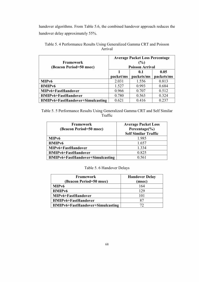
68

handover algorithms. From Table 5.6, the combined handover approach reduces the

handover delay approximately 55%.

Table 5. 4 Performance Results Using Generalized Gamma CRT and Poisson Arrival

Average Packet Loss Percentage (%)

Poisson Arrival

Framework

(Beacon Period=50 msec) 1

packet/ms0.1

packets/ms 0.05

packets/msMIPv6 2.031 1.556 0.813 HMIPv6 1.527 0.993 0.684 MIPv6+FastHandover 0.966 0.707 0.512 HMIPv6+FastHandover 0.780 0.563 0.324 HMIPv6+FastHandover+Simulcasting 0.621 0.416 0.237

Table 5. 5 Performance Results Using Generalized Gamma CRT and Self Similar

Traffic

Framework (Beacon Period=50 msec)

Average Packet Loss Percentage(%)

Self Similar Traffic MIPv6 1.985 HMIPv6 1.657 MIPv6+FastHandover 1.334 HMIPv6+FastHandover 0.825 HMIPv6+FastHandover+Simulcasting 0.561

Table 5. 6 Handover Delays

Framework (Beacon Period=50 msec)

Handover Delay (msec)

MIPv6 164 HMIPv6 129 MIPv6+FastHandover 101 HMIPv6+FastHandover 87 HMIPv6+FastHandover+Simulcasting 72

69

Figure 5. 10 Comparison of Algorithms (1 packet/msec Poisson arrival)

Figure 5. 11 Comparison of Algorithms (0.1 packet/msec Poisson arrival)

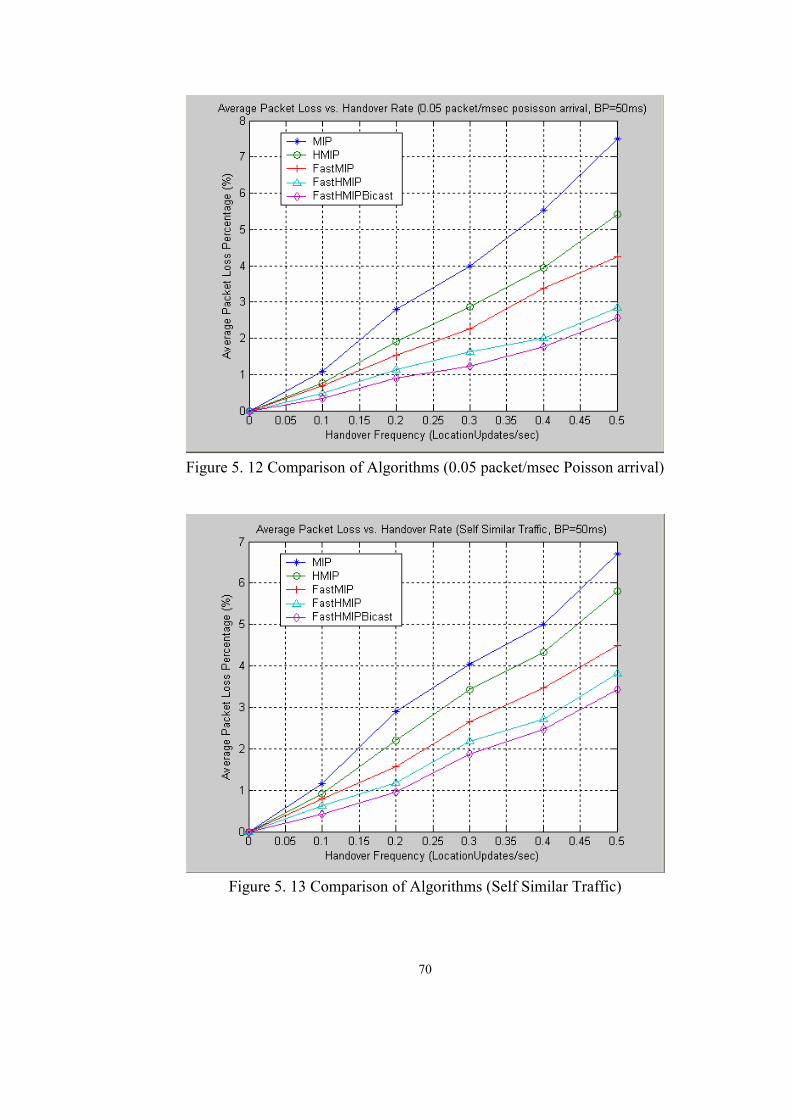
70

Figure 5. 12 Comparison of Algorithms (0.05 packet/msec Poisson arrival)

Figure 5. 13 Comparison of Algorithms (Self Similar Traffic)

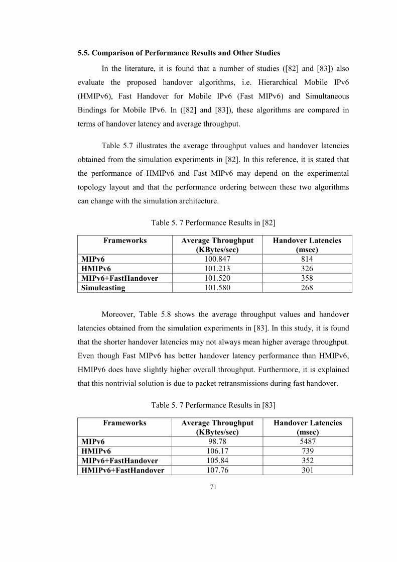
71

5.5. Comparison of Performance Results and Other Studies

In the literature, it is found that a number of studies ([82] and [83]) also

evaluate the proposed handover algorithms, i.e. Hierarchical Mobile IPv6

(HMIPv6), Fast Handover for Mobile IPv6 (Fast MIPv6) and Simultaneous

Bindings for Mobile IPv6. In ([82] and [83]), these algorithms are compared in

terms of handover latency and average throughput.

Table 5.7 illustrates the average throughput values and handover latencies

obtained from the simulation experiments in [82]. In this reference, it is stated that

the performance of HMIPv6 and Fast MIPv6 may depend on the experimental

topology layout and that the performance ordering between these two algorithms

can change with the simulation architecture.

Table 5. 7 Performance Results in [82]

Frameworks Average Throughput (KBytes/sec)

Handover Latencies (msec)

MIPv6 100.847 814 HMIPv6 101.213 326 MIPv6+FastHandover 101.520 358 Simulcasting 101.580 268

Moreover, Table 5.8 shows the average throughput values and handover

latencies obtained from the simulation experiments in [83]. In this study, it is found

that the shorter handover latencies may not always mean higher average throughput.

Even though Fast MIPv6 has better handover latency performance than HMIPv6,

HMIPv6 does have slightly higher overall throughput. Furthermore, it is explained

that this nontrivial solution is due to packet retransmissions during fast handover.

Table 5. 7 Performance Results in [83]

Frameworks Average Throughput (KBytes/sec)

Handover Latencies (msec)

MIPv6 98.78 5487 HMIPv6 106.17 739 MIPv6+FastHandover 105.84 352 HMIPv6+FastHandover 107.76 301

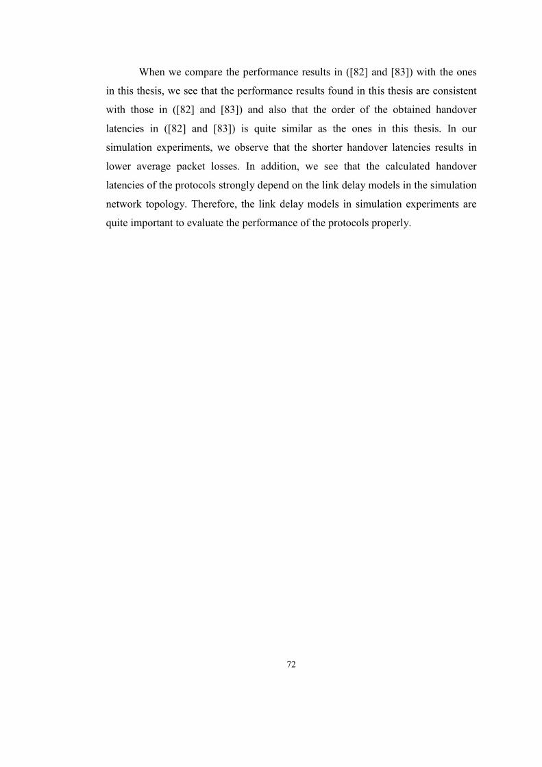
72

When we compare the performance results in ([82] and [83]) with the ones

in this thesis, we see that the performance results found in this thesis are consistent

with those in ([82] and [83]) and also that the order of the obtained handover

latencies in ([82] and [83]) is quite similar as the ones in this thesis. In our

simulation experiments, we observe that the shorter handover latencies results in

lower average packet losses. In addition, we see that the calculated handover

latencies of the protocols strongly depend on the link delay models in the simulation

network topology. Therefore, the link delay models in simulation experiments are

quite important to evaluate the performance of the protocols properly.

73

CHAPTER 6

CONCLUSIONS AND FUTURE WORK

With recent advances in wireless mobile communication technologies and

the rapid growth of the Internet, providing wireless Internet access to the mobile

users without any interruption in their connections is of crucial importance.

Enabling IP mobility in IP based networks is a significant issue for making use of

various mobile devices appearing on the Internet. In this research, we have

presented an overview of Mobile IPv6, its basic operations, main inefficiencies and

the mobility management issues at the network layer. Route optimization

mechanisms have been discussed as a means of improving the Mobile IPv6

performance. Moreover, handover algorithms for Mobile IPv6 have been surveyed

and some of the main seamless handover proposals which tend to reduce the

handover latency and packet loss have been described and evaluated. The proposed

protocols try to solve the problem of the service disruption during Mobile IPv6

handover with different methods each. However, they have also some disadvantages

and a possible combination of them is necessary in order to enhance the Mobile

IPv6 protocol. In addition, as the proposed handover algorithms are quite new, there

have not been enough research and evaluation done on these algorithms. Therefore,

a proper performance evaluation of these algorithms either by simulations or test

beds is of great significance for design issues. The performance measurements and

the results of evaluations can then be used to improve these algorithms further.

Simulation models also play a vital role in helping researchers to develop intuition.

74

In this thesis, the main performance measures for handover algorithms have

been identified as reduction in delay, packet loss, signaling in the network

architecture and also the transparency of the proposed protocol to upper layer

protocols. The algorithms proposed to enhance the performance of Mobile IPv6 are

Hierarchical Mobile IPv6, Fast Handover for Mobile IPv6 and Simultaneous

Bindings for Mobile IPv6.

Hierarchical Mobile IPv6 (HMIPv6) protocol tries to make the Mobile IPv6

handover much faster by managing micro and macro user mobility differently and

reducing the signaling between the home network and the mobile node (MN). In

order to achieve seamless handover, HMIPv6 introduces a new node called the

Mobility Anchor Point (MAP). In HMIPv6, the MN communicates with the MAP

instead of the Home Agent (HA) and the Correspondent Node (CN) to decrease the

handover latency. In case of micro mobility, i.e. the MN moves within a subnet or

within a domain, the registration requests are handled locally and not transmitted to

the HA. This reduces handover latency and location management cost. However,

this great improvement is not sufficient to provide an uninterrupted communication

during the handover. Another algorithm or a possible combination is also necessary

to perform the Mobile IPv6 handover much faster.

Fast Handover for Mobile IPv6 (Fast MIPv6) protocol proposes to reduce

the handover delay and packet loss by allowing the MN to form the new care of

address (CoA) before it attaches to the new Access Router (nAR) and forwarding

the packets destined to the MN from the old Access Router (oAR) to the nAR . This

process aims to improve the handover performance of the Mobile IPv6 protocol by

reducing handover latency. However, in Fast MIPv6 it is difficult to synchronize the

forwarding time accurately to maintain lossless communication during handover. To

solve this synchronization problem, Simultaneous Bindings for MIPv6 protocol is

proposed.

Simultaneous Bindings for Mobile IPv6 protocol enables some

enhancements for Fast MIPv6 by introducing a simultaneous binding function. The

simultaneous bindings function solves the synchronization problem of Fast MIPv6

75

by bicasting or N-casting the traffic for a short period. The goal for the simultaneous

bindings function is to reduce packet loss at the Mobile Node and to remove the

timing ambiguity regarding when to start sending traffic for the Mobile Node to its

new point of attachment following a Fast Handover. Another important goal for

simultaneous binding function is to save the MN periods of service disruption in

case of so-called ping-pong movement, i.e. when a MN moves back and forth

between two Access Routers.

In this thesis, based on this survey of handover algorithms in Mobile IPv6,

three main trends can be identified. The first trend, i.e. HMIPv6, is the widespread

use of hierarchical architectures for supporting micro mobility and reducing

signaling between the home network and the MN. The second trend, i.e. Fast

MIPv6, is forming the new CoA before the MN attaches to the nAR and forwarding

the packets destined to the MN from the oAR to the nAR. The third trend, i.e.

Simultaneous Bindings for MIPv6, is the use of various forms of multicast

capabilities in order to reduce packet loss during handovers. It is clear that we can

obtain better performance by combining these three proposed protocols. In this

thesis, the appropriate combination of the protocols, i.e. combined handover

algorithm, is also presented and described in detail. The combined handover

algorithm aims to use of hierarchical architectures, fast handover mechanisms and

simultaneous binding function together to improve the handover performance of the

standard Mobile IPv6 protocol efficiently.

In this study, the detailed performance evaluation of the handover schemes

and the combined handover method is carried out through simulations. In order to

properly predict the performance of handover extensions of Mobile IPv6, the user

mobility, the network traffic, wired and wireless links in the simulated network

topology are modeled through stochastic processes. Firstly, the network traffic is

modeled by both traditional framework modeling (termed Poisson modeling) and

self similar traffic modeling. Secondly, the user mobility is modeled by assuming

that cell residence time of the mobile user exhibits generalized gamma distribution.

76

Thirdly, the links in simulation network architecture are modeled from real traces

taken on the Internet between April and August of 2003.

Simulation results show that the HMIPv6 and the Fast MIPv6 protocols are

capable of reducing handover latency and packet loss to some extent when

compared to the standard Mobile IPv6 protocol. However, these crucial

enhancements are not sufficient to provide an uninterrupted communication to the

mobile users while roaming freely. The combined handover method that solves the

handover related issues by combining the proposed algorithms is much more

effective in terms of handover latency and packet loss compared to proposed

protocols. However, the scalability problems and the possible bottleneck problem,

i.e. the fact that all the communications within the MAP domain pass across the

MAP, of the combined handover method should also be considered in order to

provide efficient handover mechanism to the mobile users.

Another important point is that this research takes into account only the

major scenarios that might occur in wireless mobile communication environment.

These scenarios include both micro mobility and macro mobility of the mobile user.

As a future work, the other possible scenarios which need testing and simulation can

be implemented and simulated. For example, ping-pong movement of the mobile

user, i.e. when the mobile user moves back and forth between two Access Routers,

or handover to third scenario in the tunnel based fast handover might be a good

investigation so as to improve the performance of Mobile IPv6 further. In addition,

load balancing problem among multiple mobility anchor points, proper Layer 2

triggers implementations and the scalability problems of the combined handover

approach are other issues need to be investigated. Also, the ability of Mobile IPv6 to

support the mobile users roam freely between heterogeneous access technologies

and the optimal choice of the access technology suitable for services the mobile user

accesses can be investigated. Finally, in order to provide seamless service to the

mobile user and improve the efficiency of Mobile IPv6, the method that uses QoS

option in binding update messages can be studied.

77

REFERENCES

[1]T.B. Zahariadis K.G. Vaxevanakis, C.P. Tsantilas, N.A. Zervos and N.A.

Nikolaou, “Global Roaming in Next-Generation Networks”, IEEE Communications

Magazine, pp 145-151, February 2002

[2]C.E. Perkins, K. Wang, “Optimized Smooth Handoffs in Mobile IP”, Proc. Of

IEEE Symposium on Computer and Communications, Egypt, July 1999

[3]C.E. Perkins, “IP Mobility Support”, RFC 2002, IETF, October 1996

[4]H. Soliman, K.E. Malki, C. Casteluccia, L. Bellier, “Hierarchical MIPv6 mobility

management (HMIPv6)”, Internet Draft, IETF, July 2001

[5]G. Dommety, A. Yegin, C. Perkins, G. Tsirtsis, K.E. Malki, M. Khalil, “Fast

Handovers for Mobile IPv6”, Internet Draft, IETF, March 2002

[6]K.E. Malki, H. Soliman, “Simultaneous Bindings for Mobile IPv6 Fast

Handoffs”, Internet Draft, IETF, November 2001

[7]W. Leland, M. Taqqu, W. Willinger, and D. Wilson, “On the Self Similar Nature

of Ethernet Traffic (Extended Version)”, IEEE/ACM Transactions on Networking,

Vol. 2, No. 1, pp. 1-15, February 1994

78

[8]M.M. Zonoozi, P. Dassanayake, “User mobility modeling and characterization of

mobility pattern”, IEEE Journal on Selected Areas in Communications, Volume: 15,

Issue: 7, pp. 1239-1252, September 1997

[9]W. Stallings, "Wireless Communications and Networks", Prentice Hall, 2001

[10]M.Ylianttila, R. Pichna, J.Valslstrom, J. Makela, “Handoff Procedure For

Heterogeneous Wireless Networks”, Global Telecommunications Conference, 1999

[11]Nokia Networks, “Introducing Mobile IPv6 in 2G and 3G mobile Networks”,

White Paper, 2001

[12]C.E. Perkins, “Mobile IP: Design Principles and Practice”, Addisson-Wesley

Longman, Reading, Mass., 1998

[13]S. Deering, "ICMP Router Discovery Messages", RFC 1256, IETF, September

1991

[14]R. Rivest, "The MD5 Message-Digest Algorithm", RFC 1321, IETF, April 1992

[15]C.E. Perkins, "IP Encapsulation within IP", RFC 2003, IETF, October 1996

[16]C.E. Perkins, "Minimal Encapsulation within IP", RFC 2004, IETF, October

1996

[17]S. Hanks, T. Li, D. Farinacci, P. Traina, "Generic Routing Encapsulation

(GRE)", RFC 1701, IETF, October 1994

[18]D. B. Johnson and C.E. Perkins, “Route Optimization in Mobile IP”, Internet

Draft, IETF, November 1996

79

[19]P. Ferguson and D. Senie, “Network Ingress Filtering: Defeating Denial of

Service Attacks which Employ IP Source Address Spooling”, RFC 2267, IETF,

1998

[20]T. Narten, E. Nordmark, W. Simpson,"Neighbor Discovery for IP Version 6

(IPv6)", RFC1970, IETF, August 1996

[21] S. Thomson, T. Narten, "IPv6 Stateless Address Autoconfiguration", RFC1971,

IETF, August 1996

[22]S. Kent, R. Atkinson, "IP Authentication Header", Internet Draft, IETF, October

1997

[23]S. Kent, R. Atkinson, "IP Encapsulating Security Payload", Internet Draft,

IETF, October 1997

[24]S. Kent, R. Atkinson, "Security architecture for the Internet Protocol", Internet

Draft, IETF, November 1997

[25]C. Castelluccia, “Toward a Hierarchical Mobile IPv6”, Eighth IFIP Conference

on High Performance Networking, Vienna, Austria, September 1998

[26]C. Castelluccia, "A Hierarchical Mobility Management Scheme for IPv6", Third

Symposium on Computers and Communications, Athens, Greece, June 1998

[27]T. Kato, R. Takechi, H. Ono, “A Study on Mobile IPv6 Based Mobility

Management Architecture”, Fujitsu Scientific & Technical Journal, Vol. 37, pp. 65-

71, June 2001

80

[28]J.Z. Sun, J. Sauvola, “Mobility And Mobility Management: A Conceptual

Framework”, Proc. 10th IEEE International Conference on Networks, Singapore,

205-210, 2002

[29]I.F. Akyildiz, J. McNair, J. Ho, H. Uzunalioglu, W.Wang, “Mobility

Management in Next Generation Wireless Networks”, Proceedings of the IEEE,

Vol. 87, No. 3, pp. 1347-1384, August 1999

[30]F. Graziosi, M. Pratesi, M. Ruggieri, F. Santucci, “A Multicell Model of

Handover Initiation in Mobile Cellular Networks”, IEEE Trans. Veh. Technol., Vol.

48, No.3, pp. 802-814, May 1999

[31]G.P. Pollini, “Trends in Handover Design”, IEEE Commun. Mag., pp. 82-90,

March 1996

[32]Y.B. Lin, A.C. Pang, “Comparing Soft and Hard Handoffs”, IEE Trans. Veh.

Technol. Vol. 49, No. 3, p. 792-798, 2000

[33]A. Kaloxylos, S. Hadjiefthymiades and L. Merakos , "Mobility Management

and Control Protocol for Wireless ATM Networks", IEEE Network, Vol. 12, No. 4,

August 1998

[34]A. Festag, H. Karl, G. Schafer, “Current Developments and Trends in Handover

Design for ALL_IP Wireless Networks”, TKN Technical Reports Series, August

2000

[35]J. Porter, D. Gilmurray, A. Massarella, J. Naylon, “Wireless ATM Handover

Requirements and Issues”, ATM Forum/97-0153/WATM, February 1997

[36]C.E. Perkins, "Overview of Mobile IP & Seamoby", Nokia IPv6 Workshop,

September 2002

81

[37]S. Avancha, D. Chakraborty, D. Gada, T. Kamdar, A. Joshi, “ Fast and

Effective Wireless Handoff Scheme Using Forwarding Pointers and Hierarchical

Foreign Agents”, Conference on Modeling and Design of Wireless Networks,

Denver Colorado USA, August 2001

[38]Y. Xu, H.C.J. Lee, V.L.L. Thing, "A Local Mobility Agent Selection Algorithm

for Mobile Networks", IEEE International Conference on Communications,

Anchorage, Alaska, USA, Vol. 2, pp. 1074-1079, May 2003

[39]QoS Forum Publications, “QoS Protocols and Architectures”, White Paper,

http://www.qosforum.com/tech_resources.htm, 1999

[40]R. Caceres, V.N. Padmanabhan, “Fast and Scalable Handoffs for Wireless

Internetworks”, Proc. of ACM MobiCom, November 1996

[41]Sally Floyd and Vern Paxson, "Difficulties in Simulating the Internet",

IEEE/ACM Transactions on Networking, August 2001

[42]W. Willinger, “Traffic modeling for highspeed networks: Theory versus

practice”, Stochastic Networks, Vol. 71, pp. 395-409, 1995

[43]W. Willinger, M.S. Taqqu, R. Sherman, and D. V. Wilson., “Self similarity

through high-variability: Statistical analysis of Ethernet LAN traffic at the source

level”, IEEE/ACM Transactions on Networking, Vol. 5, pp. 71–86, 1997

[44]M. Crovella, A. Bestavros, “Self similarity in World Wide Web traffic:

evidence and possible causes”, IEEE/ACM Transactions on Networking, Vol. 5,

No. 6, pp. 835-846, December 1997

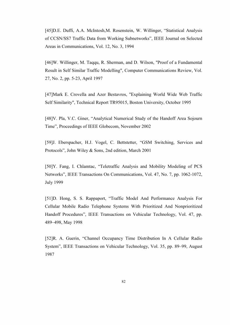
82

[45]D.E. Duffi, A.A. McIntosh,M. Rosenstein, W. Willinger, “Statistical Analysis

of CCSN/SS7 Traffic Data from Working Subnetworks”, IEEE Journal on Selected

Areas in Communications, Vol. 12, No. 3, 1994

[46]W. Willinger, M. Taqqu, R. Sherman, and D. Wilson, "Proof of a Fundamental

Result in Self Similar Traffic Modelling", Computer Communications Review, Vol.

27, No. 2, pp. 5-23, April 1997

[47]Mark E. Crovella and Azer Bestavros, "Explaining World Wide Web Traffic

Self Similarity", Technical Report TR95015, Boston University, October 1995

[48]V. Pla, V.C. Giner, “Analytical Numerical Study of the Handoff Area Sojourn

Time”, Proceedings of IEEE Globecom, November 2002

[59]J. Eberspacher, H.J. Vogel, C. Bettstetter, “GSM Switching, Services and

Protocols”, John Wiley & Sons, 2nd edition, March 2001

[50]Y. Fang, I. Chlamtac, “Teletraffic Analysis and Mobility Modeling of PCS

Networks”, IEEE Transactions On Communications, Vol. 47, No. 7, pp. 1062-1072,

July 1999

[51]D. Hong, S. S. Rappaport, “Traffic Model And Performance Analysis For

Cellular Mobile Radio Telephone Systems With Prioritized And Nonprioritized

Handoff Procedures”, IEEE Transactions on Vehicular Technology, Vol. 47, pp.

489–498, May 1998

[52]R. A. Guerin, “Channel Occupancy Time Distribution In A Cellular Radio

System”, IEEE Transactions on Vehicular Technology, Vol. 35, pp. 89–99, August

1987

83

[53]T. K. Christensen, B. F. Nielsen, and V. B. Iversen, “Distribution of channel

holding times in cellular communication systems”, Proceedings of ITC 17, pp. 471–

480, Elsevier Science, 2001

[54]H. Hidaka, K. Saitoh, N. Shinagawa, and T. Kobayashi, “Teletraffic and its self

similarities in cellular communication networks based on vehicle motion

measurements”, Proceedings of 14th ITC Specialist Seminar on Access Networks

and Systems, Spain, ITC, 2001

[55]S. Tekinay, B. Jabbari, “A measurement based prioritization scheme for

handovers in mobile cellular networks”, IEEE Journal on Selected Areas in

Communications, Vol. 10, pp. 1343–1350, October 1992

[56]C.J. Chang, T.T. Su, Y.Y. Chiang, “Analysis of a cutoff priority cellular radio

system with finite queueing and reneging dropping”, IEEE/ACM Transactions on

Networking, Vol. 2, pp. 166–175, April 1994

[57]Y.-B. Lin, S. Mohan, A. Noerpel, “Queueing priority channel assignment

strategies for PCS hand-off and initial access”, IEEE Transactions on Vehicular

Technology, Vol. 43, pp. 704–712, August 1994

[58]D. McMillan, “Delay analysis of a cellular mobile priority queuing system”,

IEEE/ACM Transactions on Networking, Vol. 3, pp. 310–319, June 1995

[59]R. Fantacci, “Performance evaluation of prioritized handoff schemes in mobile

cellular networks”, IEEE Transactions on Vehicular Technology, Vol. 49, pp. 485–

493, March 2000

[60]F. Barcelo and S. Bueno, “Idle and inter-arrival time statistics in public access

mobile radio (PAMR) systems”, Proc. IEEE Globecom’97, Phoenix, AZ, November

1997

84

[61]J. Jordan and F. Barcelo, “Statistical modeling of channel occupancy in trunked

PAMR systems”, Proc. 15th Int. Teletraffic Conf. (ITC’15), V. Ramaswami and P.

E. Wirth, Eds. Elsevier Science B.V., pp. 1169–1178, 1997

[62]P. Orlik and S. S. Rappaport, “A model for teletraffic performance and channel

holding time characterization in wireless cellular communication with general

session and dwell time distributions”, IEEE J. Select. Areas Commun., Vol. 16, pp.

788–803, 1998

[63]D. Hong, S. S. Rappaport, “Traffic Model And Performance Analysis For

Cellular Mobile Radio Telephone Systems With Prioritized And Nonprioritized

Handoff Procedures”, IEEE Transactions on Vehicular Technology, Vol. 47, pp.

489–498, May 1998

[64]Y. Fang, I. Chlamtac, “Teletraffic Analysis and Mobility Modeling of PCS

Networks”, IEEE Transactions On Communications, Vol. 47, No. 7, pp. 1062-1072

, July 1999

[65]MATLAB toolbox for statistical analysis of probability distributions,

http://www.maths.lth.se/matstat/wafo/download

[66]M. J. Luckie, A.J. McGregor, H.W. Braun, “Towards Improving Packet Probing

Techniques”, ACM SIGCOMM Internet Measurement Workshop, 2001

[67]J. Postel, “Internet control message protocol”, RFC 792, IETF, 1981

[68]S. Casner, “The mtrace manual page”, http://ftp.parc.xerox.com/pub/net-

research/ipmulti/

85

[69]V. Paxson, G. Almes, J. Mahdavi, and M. Mathis, “Framework for IP

performance metrics”, RFC 2330, IETF, 1998.

[70]G. Almes, S. Kalidindi, and M. Zekauskas, “A one-way delay metric for

IPPM”, RFC 2679, IETF, 1999

[71]S. Shalunov, B. Teitelbaum, and M. Zekauskas, “A one-way delay measurement

protocol”, IPPM work in progress, IETF, 2001

[72]G. Almes, S. Kalidindi, and M. Zekauskas, “A one-way delay metric for

IPPM”, RFC 2679, IETF, 1999

[73]W. Wu, W.S. Chen, H.E. Liao, F.F. Young, “A Seamless Handoff Approach Of

Mobile IP Protocol For Mobile Wireless Data Networks”, IEEE Transactions on

Consumer Electronics, Vol. 48, No 2, May 2002

[74]A. Mukharjee, “On the dynamics and significance of low frequency components

of Internetload”, Internetworking: Research and Experience, Vol. 5, pp. 163-205,

December 1994

[75]K. Papagianaki, S. Moon, C. Fraleigh, P. Thiran, F. Tobagi, C. Diot, “Analysis

of Measured Single Hop Delay From an Operational Backbone Network”, IEEE

JSAC Special Issue on Internet and WWW Measurement, Mapping and Modeling,

2003

[76]A. FeldMann, “Fitting Mixtures Of Exponentials To Long Tail Distributions To

Analyze Network Performance Models”, Ward Whitt Performance Evaluations,

1998

[77]A. Feldmann, “Impact Of Non Poisson Arrival Sequences For Call Admission

Algorithms With And Without Delay”, GLOBECOM, 1996

86

[78]R. Ramjee, J. Kurose, D. Towsley, “Adaptive playout mechanisms for

packetized audio applications in wide area networks”, IEEE Infocom, pp. 680-688,

June 1994

[79] R. Caceres, V.N. Padmanabhan, “Fast and Scalable Wireless Handoffs in

Support of Mobile Internet Audio”, MONET 3(4), pp. 351-363, February 1998

[80] T.T. Kwon, M. Gerla, S. Das, S. Das, “Mobility Management for VoIP Service:

Mobile IP vs. SIP”, IEEE Wireless Communication, pp 66-75, October 2002

[81] N.A. Fikouras, C. Gorg, “Performance Comparison of Hinted and

Advertisement Based Movement Detection Methods for Mobile IP Handoffs”,

Proceedings of the European Wireless 2000, Dresden, Germany, September 2000.

[82]Robert Hsieh, Aruna Seneviratne, "A comparison of mechanisms for improving

mobile IP handoff latency for end-to-end TCP", Proceedings of the 9th annual

international conference on Mobile computing and networking, ACM Press, pp. 29-

41, USA, 2003

[83]Robert Hsieh, Aruna Seneviratne, Hesham Soliman and Karim El-Malki,

“Performance Analysis on Hierarchical Mobile IPv6 with Fast-handoff”,

Proceedings of GLOBECOM, Taipei, Taiwan, 2002.