HANDBOOK ON RENEWABLE ENERGY SOURCES

Welcome message from author
This document is posted to help you gain knowledge. Please leave a comment to let me know what you think about it! Share it to your friends and learn new things together.
Transcript

HANDBOOK ON RENEWABLE ENERGY SOURCES

Handbook on Renewable Energy Sources
2
ABOUT THE PROJECT
The training handbook has been prepared by the partnership members within the frame of the SEE project called “ENergy Efficiency and Renewables–SUPporting Policies in Local level for EnergY” (ENER SUPPLY) co-financed by the European Union through the South East Europe Programme. The project aimed to reinforce the institutional capacity of the local and regional authorities in terms of planning and management of policy and actions in the field of the sustainable energy. Through the project 11 training courses have been performed in eleven countries1 of the SEE area. As whole 83 local institutions and more than 200 among employees and experts from different territories were attended to the trainings.
The training handbook itself is a final tool and it is based on the experience of this training. It has been developed by a team of experts and translated into all the languages.
For more information on the project you are invited to consult the project website: www.ener-supply.eu where you can find also the link for the e-learning platform.
The authors
BIOMASS
Prof. Giovanni Riva
He is full professor at the University Polytechnic of Marche (UNIVPM) with scientific researches in methods, technologies for energy production and saving by using biomasses. In national and international context as East Europe, Asia, Africa and South America (FAO’s framework and EU projects) he realized innovative plants and systems for data collection.
Prof. Ester Foppapedretti
She is full professor at the University Polytechnic of Marche (UNIVPM) with scientific interest in mechanical & agricultural machinery, energy and the storage of bio-products. The main research regards: study of agricultural mechanization, machines capabilities analysis, technologies used for energy sources, organic waste management study.
Phd. Carla de Carolis
She is research fellow at UNIVPM with scientific interests in LCA, Territorial planning & Biomass analysis. She studied through UE Research Programme - Marie Curie fellowship to the IFRF - International Flame Research Foundation, (Nl). Since 2007, she is working for energy research activities through UE projects of the IEE and INTERREG programme.
1 The main involved territories come from Korca e Tirana (Albania), Central Bosnia Canton (BiH), Dobrich Region, Dobrich Municipality, Dolni
Chiflik, Beloslav (Bulgaria), Split, Dalmatia County Croatia, Periphery of Peloponnese (Greece), Komárom-Esztergom County, Metropolitan Area of Budapest (Hungary), Metropolitan Area of Potenza (Italy), Ialomita County, Dambovita County (Romania), Province of Vojvodina (Serbia), Metropolitan Area of Košice (Slovakia), Ohrid, Skopje (Former Yugoslav Republic of Macedonia).

Handbook on Renewable Energy Sources
3
HYDROPOWER
Mr Eleftherios Giakoumelos
He is a Physicist (University of Patras). The last fiteen years he has worked for CRES. During his first 8 years, he worked at the Financial Services Department having as main activities the financial monitoring, control and administrative support for research programs. The last 7 years he is a member of the Training Department’s staff working in the implementation of training programs, studies and market requirement analyses.
WIND
Dr Charalambos Malamatenios
He is a Physicist (University of Patras). The last ten years he has worked for CRES. During his first 8 years, he worked at the Financial Services Department having as main activities the financial monitoring, control and administrative support for research programs. The last 5 years he is a member of the Training Department’s staff working in the implementation of training programs, studies and market requirement analyses.
GEOTHERMAL
Prof. Patrizio Signanini
He graduated in Geological Sciences in 1971 at the University of Trieste, specialized in Geophysics Applied to Hydrogeology. He has carried out assignments and activity of advising in Italy and in foreign countries He has been university professor in charge of Applied Geophysics at the University of Camerino and University of Ancona. Since 2001 he is Scientific Leader of Research agreement with Lotti Associati S.p.A. about water reservoir in subtropical area. He is the Author of about 50 scientific papers.
Mr Crema Giancarlo
He graduated in Geological Sciences in 1963 and in Chemistry in 1968 at the University of Torino. He has been analyst and researcher about rocks, water and soil at the University of Torino and worked as supervisor and director of many works in Italy. He has been university professor of Hydrogeology at the University of Camerino. Since 1994 he is Professor of Applied Hydrogeology and Environmental Hydrogeology at University of Chieti-Pescara. He is the Author of about 50 scientific papers.
Mrs Micaela Di Fazio
She graduated in Geological Sciences at the University “UNIROMA 3” of Roma and graduated in Geological Sciences (graduate specialist) in 2009 at the University “G. D’Annunzio” of Chieti - Pescara. She is Phd student at the University “G. D’Annunzio” of Chieti - Pescara since 2010, she collaborates with the Institute for Advanced Biomedical Technologies (ITAB) and body of the State Forestry to perform thermographic surveys on the ground and by helicopter on contaminated sites, landfills.

Handbook on Renewable Energy Sources
4
FINANCIAL EVALUATION
Prof. Jozef Gajdoš
He graduated at University of Economics Faculty of Business Administration. He has 24 years of experience in: Logistic, Project management, Economic and Financial Analysis. He has worked, since 1990 at University of Economics in Bratislava (Slovakia), Faculty of Business Administration in Košice, as assistant professor with specialization in Logistics. He is the author of about 30 scientific papers.
Prof. Rastislav Ručinský
He graduated at University of Economics Faculty of Business Administration. He has 9 year of experience in Project management, Economic and Financial Analysis. He is Vice-dean for Development, Informatization and Public Relations and assistant professor at Faculty of Business Administration in Košice, University of Economics in Bratislava (Slovakia). He finished PhD studies in 2004 at the same University. He specialized in Project Management and Finance. He is the author of about 30 scientific papers.

Handbook on Renewable Energy Sources
5
ACKNOWLEDGEMENT
ENER SUPPLY project has additionally benefitted from the generous contribution of time and knowledge from a wide group of individuals. It would not have been possible without this. This group includes among the others: Prof. Knezevic, Phd Masa Bukurov, Arch. Margareta Zidar, Eng. Patrizia Carlucci, Phd Jana Nascakova.
The coordination and the planning activities during the development of the handbook and all the training activity has been taken care by Marco Caponigro and Azrudin Husika.
In particular, a group of persons deserves special mention. The employees of Local and Regional Authorities that took part at the training courses in all the South East Europe during the ENER SUPPLY project, thanks to their participation, comments and observations it was possible to review and adapt all the materials. The JTS that recognised the potential value of this project and became a door opened to the discussion.
Tragically, Ilian Katesky passed away in November 2011. His initial support during my time in Bulgaria, his sense of humour and light sense of life will be missed by his many friends and colleagues.
Marco Caponigro
Disclaimer
The authors take full responsibility for the information and views presented in this handbook. These views do not represent the views or positions of the European Commission, co-funder of the project. While this works strong points undoubtedly have benefitted from the insights of many others, any errors and omissions rest entirely with the authors.
Handbook on Renewable Energy Sources
6
INTRODUCTION
The acceleration of GHG emissions indicates a mounting threat of runaway climate change, with potentially disastrous human consequences. The utilization of Renewable Energy Sources (RES) together with improvement of the energy end-use efficiency (EE) can contribute to the reduction of primary energy consumption, to the mitigation of GHG emissions and thereby to the prevention of dangerous climate change2.
Thenot utilized potential of biomass, solar, hydro, wind and geothermal source is still high. However in the recent years due significant public incentives in the form of feed-in-tariff, in many European countriesthe development of the sector has progressively increase.
EU adopted its own strategy to fight the climate change till the adoption of a plan for a sustainable growth Europa 2020 in which it set ambitious objectives in terms of energy (the so called 20-20-20).Moving towards a low-carbon economy requires a public sector able to identify and support the economic opportunities. In particular the local public sector can play a strategic role as manager of the territory and last implementer of public policies. Therefore in the field of sustainable energy, it is essential to reinforce the capacities of the local public sector through the empowerment of its workforce.
This is the key objective of the handbook: strengthen part of the skills and competences in the field of planning and management of RES. The textbooks extensively, rely on the different methodology, is organised on four sections, one for each main renewable energy sources:
(1) biomass, (2) geothermal, (3) hydropower, (4) wind energy.
The aim of the handbooks is to present a good overview of the RESs, main technological development, and case studies together with applicable example of utilization of sources. The text tends – if available – also to focus on possible planning concepts like how to set up a map to identify and provide a first dimension of the potential of each sources and also how to implement feasibility study. The information is based on relevant international body of knowledge. The publication includes at the end a brief annex related the financial evaluation especially useful for those unfamiliar with it.
Our wish is that this work can contribute to overcome the existing barriers in the development of the RES.
Marco Caponigro Azrudin Husika
2Human activities attributed to the energy sector cause as much as 78 % of the Community greenhouse gas emissions (Directive 2006/32/EC of
the European Parliament and of the Council of 5 April 2006on energy end-use efficiency and energy services and repealing Council Directive 93/76/EEC).
Handbook on Renewable Energy Sources
7
TABLE OF CONTENTS
BIOMASS ENERGY
1. BACKGROUND ...................................................................................................................................................... 12
2. BIOMASS AND SUSTAINABILITY ........................................................................................................................ 12
2.1 Biomass definition .............................................................................................................................................. 12
2.2 Biomass and Sustainability ................................................................................................................................ 13
2.3 EU Sustainability Scheme for Biofuels .............................................................................................................. 15
3. BIOMASS ................................................................................................................................................................ 16
3.1 Types of Biomass ................................................................................................................................................ 16
3.1.1 Biomass by energy crops .................................................................................................................................. 16
3.1.2 Biomass by Residues and Wastes .................................................................................................................... 19
4. ANALYSIS AND ESTIMATION OF BIOMASS PRODUCTION .............................................................................. 23
4.1 Biomass Classification ....................................................................................................................................... 23
4.2 Estimation of the biomass potential ................................................................................................................. 24
4.3 Calculation of Potential Biomass ...................................................................................................................... 25
4.3.1 Biomass potential by energy crops .................................................................................................................... 25
4.3.2 Biomass potential by residuals and wastes ........................................................................................................ 29
4.4 Calculation of Available Biomass ..................................................................................................................... 34
5. BIOMASS ENERGY CONVERSION: TECHNOLOGIES OVERVIEW .................................................................. 35
5.1 Integration between technologies: general aspects........................................................................................ 37
6. CONCLUSION ....................................................................................................................................................... 38
HYDROPOWER
1. INTRODUCTION ..................................................................................................................................................... 40
1.1 Basic definitions and processes ........................................................................................................................ 40
1.2 Advantages of small-hydro ................................................................................................................................. 41
2. HYDROPOWER BASICS ........................................................................................................................................ 42
2.1 Head and flow ...................................................................................................................................................... 42

Handbook on Renewable Energy Sources
8
2.2 Power and Energy ............................................................................................................................................... 42
2.3 Main elements of a small hydropower scheme ................................................................................................. 43
3. TECHNOLOGY ....................................................................................................................................................... 44
3.1 Overview ............................................................................................................................................................... 44
3.2 Types of turbines suitable for SHP .................................................................................................................... 44
3.3 Turbine selection criteria .................................................................................................................................... 46
3.4 Turbine efficiency ................................................................................................................................................ 47
3.5 Control .................................................................................................................................................................. 48
3.6 Screening ............................................................................................................................................................. 49
4. RESOURCE ASSESSMENT ................................................................................................................................... 51
4.1 Introduction .......................................................................................................................................................... 51
4.2 National and regional levels ............................................................................................................................... 52
4.3 Resource estimation at local levels (site specific) ........................................................................................... 54
5. CRES METHOD FOR THE ASSESSMENT OF SMALL HYDRO POTENTIAL ..................................................... 57
5.1 General concept .................................................................................................................................................. 57
5.2 Description of the geographical system’s database ........................................................................................ 58
5.3 Methodological approach for calculating the exploitable potential of HPS ................................................... 61
5.4 Digital terrain model and water streams ............................................................................................................ 62
5.5 Topological water stream model ........................................................................................................................ 62
5.7 Energy production by Small Hydro plants ........................................................................................................ 65
6. COMMISSIONING A FEASIBILITY STUDY ........................................................................................................... 68
6.1 Preliminaries ........................................................................................................................................................ 68
6.2 Feasibility ............................................................................................................................................................. 68
WIND ENERGY
1. THE WIND IN THE WIND ENERGY ....................................................................................................................... 71
1.2 Rated power of a WT ........................................................................................................................................... 72
1.3 Power extraction by a wind turbine ................................................................................................................... 73
1.4 Variability of the wind .......................................................................................................................................... 75
1.5 Variation with time .............................................................................................................................................. 76

Handbook on Renewable Energy Sources
9
2. WIND RESOURCE ASSESSMENT ........................................................................................................................ 77
2.1 Introduction .......................................................................................................................................................... 77
2.2 Determination of site conditions ........................................................................................................................ 77
2.3 Procedure ............................................................................................................................................................. 79
3. WIND SPEED PROFILES & MEASUREMENTS .................................................................................................... 81
3.1 Wind speed profiles ............................................................................................................................................ 81
3.2 Wind speed measurements ................................................................................................................................ 82
3.3 Presentation of archived data ............................................................................................................................ 85
3.4 Analysis of on-site data ...................................................................................................................................... 87
4. ESTIMATION OF ENERGY PRODUCTION ........................................................................................................... 89
4.1 Calculation of AEP with the use of a measured wind speed histogram ......................................................... 89
4.2 Calculation of AEP using a theoretical wind speed distribution ..................................................................... 90
5. SITE FACTORS THAT AFFECT THE SELECTION ............................................................................................... 91
5.1 Site access ........................................................................................................................................................... 91
5.2 Grid integration .................................................................................................................................................... 92
5.2.1 Public electricity transmission & distribution system ........................................................................................... 92
5.2.2 Design of the connection .................................................................................................................................... 93
5.3 Other issues affecting the selection of the site ................................................................................................ 94
5.3.1 Issues concerning local communities ................................................................................................................. 94
5.3.2 Avoiding wildlife and other sensitive areas ......................................................................................................... 97
5.4 Planning for wind development ......................................................................................................................... 99
6. CRES WIND ATLAS METHODOLOGY AND APPLICATION RESULTS ............................................................ 100
6.1 Introduction ........................................................................................................................................................ 100
6.2 Description of the methodology ....................................................................................................................... 100
GEOTHERMAL ENERGY
1. GEOTHERMAL ENERGY AND THE ENVIRONMENT ......................................................................................... 103
1.1 Environmental benefits of geothermal energy ................................................................................................ 104
1.2 Geothermal temperature gradient .................................................................................................................... 104

Handbook on Renewable Energy Sources
10
2. BACKGROUND ON GEOTHERMAL ENERGY .................................................................................................. 106
2.1 Geothermal Systems ........................................................................................................................................ 106
2.2 Concept of Enthalpy .......................................................................................................................................... 107
3. UTILIZATION OF GEOTHERMAL RESOURCES ................................................................................................ 108
3.1 Direct heat uses ................................................................................................................................................ 109
3.1.1 Principles of heat pumps .................................................................................................................................. 109
3.2 Electricity generation ........................................................................................................................................ 110
4. RESEARCH OF GEOTHERMAL RESOURCES .................................................................................................. 112
4.1 Exploration methods ......................................................................................................................................... 112
4.1.1 Requested input data........................................................................................................................................ 113
4.1.2 Availability of input data in different countries ................................................................................................... 114
4.1.3 Methodology of development of RES maps ...................................................................................................... 115
4.1.4 Example of one RES Map ................................................................................................................................ 117
ANNEX: FINANCIAL EVALUATION OF RENEWABLE ENERGY PROJECTS
1. INTRODUCTION ................................................................................................................................................... 144
2. ECONOMIC ASPECTS OF RENEWABLE ENERGY SOURCES EVALUATION ............................................... 144
2.1 Basic concepts ................................................................................................................................................. 144
2.2 Basic methods for natural resources evaluation ............................................................................................ 145
2.3 The basic economic problems ......................................................................................................................... 146
2.4 Cost–benefit analysis ........................................................................................................................................ 150
2.5 Economic impact analysis ............................................................................................................................... 151
2.6 Alternative capital budgeting methods ............................................................................................................ 152

Handbook on Renewable Energy Sources
11
BIOMASS ENERGY

Handbook on Renewable Energy Sources
12
1. Background
This report is a tool for the local training foreseen as part of the activities of the European
Project ENER SUPPLY. It takes in consideration different aspects about sustainability,
innovation, engineering and science. It’s focussed on different aspects about biomass
background as: definition and classification; evaluation of potential and available sources,
technological options for biomass using; it also provides guidelines for addressing critical issues
and for identify major strategic opportunities. These items are presented by the following macro-
sections:
Biomass and Sustainability
Biomass Resources classification
Biomass evaluation
Biomass Processing Technologies
Evaluating and Monitoring Bioenergy Projects
Sections from 1 to 3 are finalized to analyse sustainability and biomass production issues. Key
information for understanding the details of specific technologies are provided in section 4.
Section 5 integrates the findings into a sustainability analysis tool designed to assist projects,
with a summary the major strategic relationships with regards to the development of sustainable
bioenergy opportunities.
2. Biomass and Sustainability
Biomass considered as an energy resource is fundamentally different from carbon free energy
sources (i.e.: wind). It could generate energy and material products similar to the traditional
ones produced by existing fossil fuel uses. Biomass has also a very important utilisation as food
and as raw materials for industry which must be correctly integrated with the energy use to
respect the sustainability principles which will be discussed in the following sections.
2.1 Biomass definition
According to the definition given by Directive 2009/28/CE, biomass is "the biodegradable
fraction of products, waste and residues from biological origin from agriculture (including vegetal
and animal substances), forestry and related industries including fisheries and aquaculture, as
well as the biodegradable fraction of industrial and municipal waste"3.
This means that with appropriate industrial processing, newly harvested biomass can be
converted into homolog of natural gas and of liquid and solid fossil fuels. By using various
3 As defined under Article 2(e) in Directive 2009/28/EC

Handbook on Renewable Energy Sources
13
transformation processes such as combustion, gasification and pyrolysis, biomass can be
transformed into “bio-fuels” for transport, “bio-heat” or “bio-electricity”.
2.2 Biomass and Sustainability
The use of bioenergy is related to the impact on land use. ‘Renewable’, ‘Low greenhouse gas
emission’ and ‘Sustainable’ are not synonymous terms and must be considered one by one, in
the biomass projects.
More in details, the “Sustainability” is fulfilled when project based on renewable sources has a
negative or, at least, neutral CO2 balances over the life cycle.
The biomass chain could be characterized by carbon negative balance (net removal of CO2eq.
from the atmosphere) as well as carbon positive balances (net addition of CO2eq.): this depends
on field practices, transport and processing technologies 4(BCT, 2007).
The GHG emissions represent one of the environmental criteria included in a sustainability
analysis, but it’s not sufficient. The sustainability concept has to include in the evaluation also
other different aspects as ecological, cultural and health and has to be also integrate with
economic aspects (Fig. 2).
From a general point of view, the concept of sustainability applied to bioenergy sector cannot be
therefore untied from Environmental, Economic and Social aspects, as pictured below (Fig. 1,
Fig. 2). If one of these aspects is not included, it could belong to equitable, bearable or viable
conditions, but not sustainable.
Then, biomass projects will not be completely successful unless they can demonstrate
sustainable biomass supply, viable business conditions and social support, as summarised
below (Tab.1).
The concept of biomass evaluation has undergone remarkable evolution thanks to RED
2009/208/CE. At the beginning, the biomass estimation for a territorial planning was based on
potential biomass values, going on, it was based on available biomass values; now, according
to the RED directive, it’s necessary to do a step towards to the evaluation of “Sustainable
Biomass”. Not all available biomass can be sustainable.
4 A carbon negative balance is achieved if the standing stock of biomass increases or carbon is removed from the carbon cycle via inactive soil
carbon, pyrolysis char or carbon capture and storage.

Handbook on Renewable Energy Sources
14
Figure 1. – General Concept of sustainable approach, (Adams W.M., 2006)
Figure 2. - General approach for a Bioenergy project

Handbook on Renewable Energy Sources
15
Table 1. – Hierarchy of sustainability considerations for biomass projects (Crucible Carbon, 2008).
Sustainability Criteria Aspects evaluated
Ecologically sustainable and viable biomass supply
- Land Availability
- Water Availability
- Biodiversity
Commercially and Technologically Viable Processing Business
- Feedstock Supply
- Technology
- Products and Market
Licence to operate
- Government Directives
- Community Directives
- Public Consensus
In conclusion, producing energy from renewable sources in sustainably ways is also a social
challenge that entails an evolution of the international and national rules (as in part started with
the RED 2009/28/CE), a planning both for urban and transport sectors and a changing of the
individual lifestyles and ethical consumerism.
2.3 European Union Sustainability Scheme for Biofuels
The benefits of biofuels over traditional fuels include greater energy security, reduced
environmental impact, foreign exchange savings and socioeconomic issues related to the rural
sector. The concept of sustainable development embodies the idea of the inter-linkage and the
balance between economic, social and environmental concerns, (Demirbas A., 2009).
As a consequence of to EU level, with the resolution of 25 September 2007 on the Road Map
for Renewable Energy in Europe, the European Parliament stressed the importance of
sustainability criteria for biofuels and requested the Commission to undertake action to build a
mandatory certification system for biofuels.
In with the publication of RED Directive (2009/28/EC), the environmental sustainability criteria
and verification requirements for biofuels and other bioliquids have been included.
The Commission has also asked to focus on standards needed for the implementation of the
Directive 2009/28/CE and a standardisation activity is ongoing within CEN (CEN Technical
Committee 383) for the definition of sustainably produced biomass for energy applications.
With the last Directive of sustainability criteria for Biomass uses, the European Commission has
introduced the most comprehensive and advanced sustainability scheme and the Member
States are responsible to confirm and implement them for biofuels/bioliquids produced in the
UE. Another important point of the sustainable criteria scheme is the land typology. In particular,
biofuels couldn’t be produced in lands in high biodiversity value lands. Raw material should not
be obtained from primary forest, or from designated nature protection areas, or from high
biodiversity grasslands. The Commission will define the criteria and geographic ranges to
identify high biodiversity grasslands.
Other sustainable criterion considered by RED directive is the high level of carbon stock: raw
materials should not be obtained from wetland, continuously forested areas and from areas with
10-30 % canopy cover and peat-land.
Handbook on Renewable Energy Sources
16
Finally the Red Directive examines the biofuel coming only partly from non-renewable sources.
For some of them, such as ETBE, the RED Directive indicates which percentage of fuel is
renewable on the purpose of target accounting.
For the not listed fuels, (including fuels produced in flexible processes, with different mix of
sources, i.e. co-firing system), analogy can be appropriately drawn from the rule for electricity
generated in multi-fuel plants: the contribution of each energy source have to be taken into
account on the basis of its energy content.
3. Biomass
The bio-energy chains of given territory have to be realized considering the technologies and
the biomass types to achieve the best outcomes. Classification and peculiarity of the different
biomass resources therefore have to be known.
This section contents the general biomass description and its connections to the processing
conditions. At the same time, it highlights the biomass features which can have more influence
on the sustainability scheme and their use for bioenergy applications.
3.1 Types of Biomass
The overwhelming majority of biomass available for bioenergy is derived from plant material
also that from animal products.
Some of the important features of different biomasses are presented below. A first distinction
can be made considering the origin of the biomass from the different sectors such as:
agricultural sector, forestal, industrial and urban sectors. Another classification can be as well
as by its nature can be represented by both energy crops or residues and wastes.
3.1.1 Biomass by energy crops
The biomass represented by energy crops is obviously coming by agricultural and forestal
sectors.
Annual Grassy Crops
Grassy (monocotyledon) plants form the bulk of modern broad scale agriculture. Annual grassy
crops include cereal as grains, barley, oats, rye and other minor cereals; sugar beet, sugar
cane; forage crops, as clover grasses species.
Seeds from these cereals crops, tuber and stem of other plants tend to be a good source of
starch which can be used by technological processes for biofuels or energy production.
Selective breeding (particularly for “no food crops”) has been used to alter the seed/plant
biomass ratio in many species which with large increases in seed yield.
Handbook on Renewable Energy Sources
17
Perennial Grassy Crops
This type of biomass can be used as bioenergy feedstock when the economics are viable. Fast
growing reeds and canes (such as Arundo Donax, Elephant grasses) are examples of grassy
crops that can make good use of nutrient availability to increases biomass productivity; but at
the same time, some other agronomic characteristics represent yet weak points such as floral
sterility, prohibitive cost for crop establishment, low relative harvest mechanization, high
moisture during harvestable product and high ash content. (Ranalli P., 2010).
Cardoon and Mischantus are other energy crops with the Mediterranean characteristics of
growing with low water: for this reason, they are obtaining high interest and research activities in
agronomic and genetic fields with programmes of improvement.
Oil Crops
Oil crops include Annual oil-seed crops and Perennial oil-tree crops.
Oil Seed Crops
From an agronomic point of view, the oil seed crops have an evolutionary history different form
cereal crops and therefore can have an additional benefit as a break crop in reducing plant soil
pathogens.
The most representative oil crops in European areas are rapeseed and sunflower. Vegetable oil
is usually extracted through mechanical pressing and/or solvent and is used for food
preparation, soaps and cosmetics. Oil in these crops usually contains other seed constituents
(protein or starch) as part of the crop revenue stream. The lignocellulose part of oil crops,
which is traditionally used as mulch or fodder, can also be combusted for heat and power, while
vegetable oils can be used for higher value bioenergy applications, especially as a diesel
replacement (Crucible Carbon, 2010).
Vegetable oils deriving from these crops and modified in m-ethyl esters are commonly called
‘‘biodiesel” and prominent candidates to become alternative diesel fuels.
Oil Tree Crops
Actually, a number of tree crops produce oil: palm, coconut and macadamia. Palm oil in
particular is used in the developed countries to produce both edible oil than primary products for
biodiesel.
But extensive use of edible oils may cause significant problems such as starvation in developing
countries. The twofold use of palm oil increases the competition between edible oil market and
biofuels market with a consequent increase of vegetable oil price in the developing countries.
The use of non-edible plant oils, when compared with edible oils, is very significant in
developing countries because of the tremendous demand for edible oils as food and they are far

Handbook on Renewable Energy Sources
18
too expensive to be used as fuel at present. The production of biodiesel from different non-
edible oilseed crops has been extensively investigated over the last few years5 (Balat M., 2010).
Oil tree crops with their lower food values can be a resource for bioenergy and, as perennials
crops, provide water and carbon sink benefits. Non-food crops will also not display spikes in
value associated with food supply and demand issues. Many food oil producing species, such
as Jatropha (in subtropical areas), can be useful for bioenergy and are often promoted as not
competing with food crops. However these species can display many properties associated with
weeds and can become subject to bans in order to limit infestation risks (Crucible Carbon,
2008).
The problem of great concern regards the rate of vegetative growth and seed yield (Balat M.,
2010).
Table 2. - Comparison between different oil crops for Biodiesel production (Balat M., 2010)
Oil Crops Oil production (t/ha) Reference
Rapeseed 1 M.Balat, 2010
Soybean 0.52 M.Balat, 2010
Sunflower 0.9 Foppa Pedretti et al., 2009
Palm 5 M.Balat, 2010
Jatropha3 0.5 M.Balat, 2010
Microalgae 50 M.Balat, 2010
Lignocellulosic Crops
Corn and soybeans are annuals, differently forms of lignocellulosic bioenergy crops are typically
perennials.
Lignocellulosic crops include perennial grassy crops and others tree crops.
Herbaceous species include crops as: Switchgrass, Panicum virgatum; Phalaris Arundinacea
and Miscanthus (Miscanthus spp.)
Hardwoods species include woody species such as willows Salix spp., Poplars Populus spp.,
Eucalyptus, others. Among them, Poplar, Miscanthus and Switchgrass have received particular
attention for their high biomass yield, efficient nutrient utilization, low erosion soil potential,
carbon sequestration capability and reduced fossil fuel input requirements in comparison with
annual crops, (Abbasi T. et al, 2009).
Several research activities have been carried out on poplar which is considered one of the most
important plants for its short rotation: this has permitted to develop important genetic
programmes with an increase of varieties and clones, exportable around the world. Other
woody crops as Eucalyptus let produce biomass at warmer conditions, as Mediterranean
climate (Ranalli P., 2010).
5 The production of biodiesel from different non-edible oilseed crops has been extensively investigated over the last few years. Some of these
non-edible oilseed crops include Jatropha tree (Jatropha curcas), Karanja (Pongamia pinnata) , Tobacco seed (Nicotiana tabacum L.) , Rice bran
, Mahua (Madhuca indica), Neem (Azadirachta indica), Rubber plant (Hevea brasiliensis), Castor, Linseed, and Microalgae, etc.

Handbook on Renewable Energy Sources
19
3.1.2 Biomass by Residues and Wastes
The analysis of biomass by residues and wastes is more complicated for the complexity of the
materials managed and the different sectors of origin (i.e.: from agriculture to urban sector).
At first, UE Directive 2008/98/CE defines a difference between co-products and wastes: “Co-
product all material that can be re-used while waste is defined as material reached to the end of
production cycle and cannot be re-cycled” (Castelli S., 2010).
Waste materials are generated in manufacturing processes, industries and municipal solid
wastes; the typical energy content is from 10.5 to 11.5 MJ/kg.
Waste management practices differ for developed and developing nations, for urban and rural
areas and for residential and industrial producers.
The starting situation of a developing country in waste management differs from that of
industrialized countries. The transfer of proven technology from one country to another can be
quite inappropriate although technically viable or affordable. It’s very important to understand
the local factors such as:
- Waste characteristics and seasonal variations in climate
- Social aspects, cultural attitudes towards solid waste and political institutions
- Awareness of the more obvious resource limitations which often exist.
The role of sustainable waste management is to reduce the amount of waste that is discharged
into the environment by reducing the amount of waste generated. Large quantities of waste
cannot be eliminated. However, the environmental impact can be reduced by making more
sustainable use of the waste. This is known as the ‘‘Waste hierarchy”.
The waste hierarchy refers to reduce, reuse and recycle and classify waste management
strategies according to their desirability in terms of waste minimization. The aim of the waste
hierarchy is to extract the maximum practical benefits from products and to generate the
minimum amount of waste (Demirbas A., 2010).
Part of biomass is also classified as waste deriving from industrial, agricultural, forestal and
urban activities: it is simple to apply the “waste hierarchy” concept to all wastes or residuals
included in the biomass sector, as showed in the following section.
Potential biomass based residues and wastes include plants and animal residues. They are
represented by agricultural residues such as straw, vegetable/ fruit peels; forestry residues and
wastes such as leaf litter and sawmill food wastes and biomass components by municipal solid
wastes. Energy can be produced from these wastes because, globally, several billion tonnes of
biomass is contained in them. (Abbasi et al, 2009).
There are various options available to convert residues or waste to energy. The technologies
are sanitary landfill, incineration, pyrolysis, gasification, anaerobic digestion and others. Short
informations will be given for each one in this section; further descriptions will be given in
section 5.

Handbook on Renewable Energy Sources
20
The choice of technology has to be based on the waste typology, its quality and the local
conditions; but a classification and assignment of different wastes is not easy. In UE countries,
the wastes are classified with a “EWC Code”6, (EPA, 2002). Table 5 shows a general scheme of
promising waste treatment processes.
Table 3. - Waste processes (Demirbas A., 2010)
Type of Waste Waste disposal method
Combustible Waste
Roaster incineration
Fluid bed incineration
Pyrolysis–incineration
Pyrolysis–gasification
Separation–composting–
Incineration
Separation-pyrolysis
Separation-gasification
Separation-incineration in a cement plant
(Wet and dry) separation-digest-incineration in a cement plant
Non-Combustible Wastes Landfill
Partially combustible
waste streams
Wood
Pyrolysis and co-incineration in a coal
power plant
Pyrolysis and co-incineration in a coal power plant
Incineration in a fluid bed furnace
gasification
Plastics Gasification
Feedstock recycling
Fermentable Organic
Wastes
Composting
Anaerobic digestion
The best compromise would be to choose the technology, which has the lowest life cycle cost,
needs the least land areas, causes practically no air and land pollution, produces more power
with less waste and causes maximum volume reduction, (Demirbas A., 2010).
Nowadays, to obtain the energy in a clean and cost effective manner is a major challenge yet to
be met. Actually, one of the biggest problems is to find how to convert quickly and economically
convert the lignocellulosic components of these wastes into simpler sugars to enable their
subsequent biochemical conversion to clean fuels (Abbasi M. et al, 2009).
6 EWC is European Waste Catalogue that is used for classification of all wastes and hazardous wastes. It is designed to form a consistent waste
classification system across the EU for disposal and recovery. The new codified Waste Framework (Directive 2006/12/EC), is now the only legally valid version.

Handbook on Renewable Energy Sources
21
Recently, producing energy and biofuels by wastes and residues is obtaining considerable
importance for the positive environmental and economical effect. Using organic urban wastes
for energy purpose would avoid an enlargement of urban landfills with a consequent reduction
of GHG emissions and more independence from utilization of fossil fuels.
At last point but not least, it is also important to recognise that wastes often contain both energy
and nutrient components.
A basic rule for ecological sustainability is that energy may be extracted from
production/consumption systems but nutrients must be recycled. It is not advisable to base a
bioenergy project on waste streams that should be minimised or converted to higher value
outcomes, (Crucible Carbon, 2008).
Biogenic wastes from urban and industrial sectors
Wastes from industrial and municipal sources is an attractive biomass source (especially if the
organic fraction called biogenic fraction is considered), because the material has already been
collected and can be acquired at a negative cost, due to tipping fees (i.e., sources will pay
money to get rid of waste) (Demirbas A., 2010).
On the basis of the “Waste hierarchy” concept, to re-use part of the biogenic fraction of
municipality and industrial wastes could be an interesting biomass for energy recovery by
anaerobic digestion process.
A particular consideration has to be done on the use of Waste Cooking Oil for biofuel
production. The production of biodiesel from waste cooking oil to partially substitute petroleum
diesel is one of the measures for solving the twin problems of environment pollution and energy
shortage.
Residues and wastes from agricultural sector
Major agricultural residues include crop residues, straws and husks, olive pits and nut shells.
More in particular, the residue can be divided into two general categories:
- Field residues: material left in the fields or orchards after harvesting as stalks, stems, leaves
and seed pods.
- Process residues: materials left after the processing of the crop into a usable resources
husks, seeds, bagasse and roots.
Some agricultural residues are used as animal fodder, for soil management and in
manufacturing.
The stover is the above ground portion of the corn plant, other than grain and consists of stalk
(including tassel), leaves, cob, husk and silks. On average, the dry matter weight of a corn plant
is split equally between the grain and the stover. Currently, about 5% stover is used for animal
bedding and feeding and the remaining is ploughed into the soil or burned as activity practiced
for straw disposal, but due to energy content of straw, many UE countries are using it for energy
purposes.
Handbook on Renewable Energy Sources
22
Residues and wastes from forestal sector
Still now, most of the wood derived from forestal sector is a predominant source in non-OPEC
and developing countries and it’s also used as principal fuel for small scale energy production in
rural areas where gas fuel is not common. It well competes with fossil fuel and it is used both in
the houses for cooking and water heating and in commercial and industrial processes (for water
heating and process heat).
Alternative use of wastes from forestry or industrial activities connected as sawmill, represents
an attractive source of biomass and a successful example for energy production by residues.
The forestal residues are cutting wood, logging residues, trees, shrubs, bark and etc. (Demirbas
A, 2000).
Normally, forest wood residues are considered better fuels than agricultural residues but their
density value and harvest system (above all when slope of the soil is high) keep high their
transport costs; the net-CO2 emission produced for every unit energy delivered by forest logging
residues is lower than that produced by other agricultural residues, due to fertilizers and
pesticides utilized (Borjesson P, 1996).
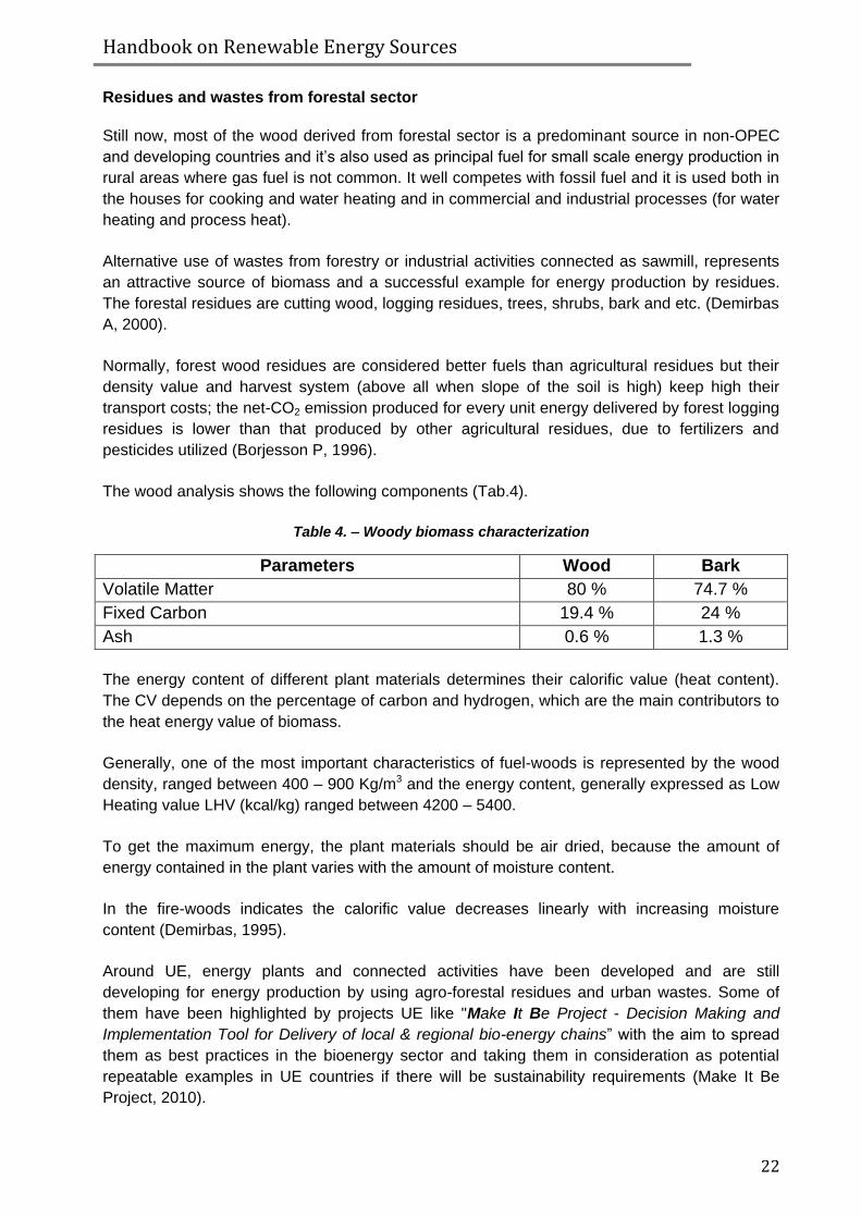
The wood analysis shows the following components (Tab.4).
Table 4. – Woody biomass characterization
Parameters Wood Bark
Volatile Matter 80 % 74.7 %
Fixed Carbon 19.4 % 24 %
Ash 0.6 % 1.3 %
The energy content of different plant materials determines their calorific value (heat content).
The CV depends on the percentage of carbon and hydrogen, which are the main contributors to
the heat energy value of biomass.
Generally, one of the most important characteristics of fuel-woods is represented by the wood
density, ranged between 400 – 900 Kg/m3 and the energy content, generally expressed as Low
Heating value LHV (kcal/kg) ranged between 4200 – 5400.
To get the maximum energy, the plant materials should be air dried, because the amount of
energy contained in the plant varies with the amount of moisture content.
In the fire-woods indicates the calorific value decreases linearly with increasing moisture
content (Demirbas, 1995).
Around UE, energy plants and connected activities have been developed and are still
developing for energy production by using agro-forestal residues and urban wastes. Some of
them have been highlighted by projects UE like "Make It Be Project - Decision Making and
Implementation Tool for Delivery of local & regional bio-energy chains” with the aim to spread
them as best practices in the bioenergy sector and taking them in consideration as potential
repeatable examples in UE countries if there will be sustainability requirements (Make It Be
Project, 2010).

Handbook on Renewable Energy Sources
23
4. Analysis and estimation of Biomass production
The availability of biomass for a given territory permits to estimating at estimating how much
bio-energy can contribute to the energy supply. This section provides to define the potentiality
and the availability of biomass in sustainability conditions in several sectors (agriculture,
forestry, industry and wastes) as listed before.
The analysis of biomass production will be adopted for the studied regions according to each
specific situation: some UE regions will have a sector more developed than others.
In a preliminary analysis the amount of biomass can be converted from tonnes per year to an
energetic unit such as Joules or kWh or TOE.
It is important to underline that, the specific energy conversion and relative technology has not
been chosen yet but they will be considered in the section.
4.1 Biomass Classification
To estimate the biomass of specific territory needs, at first, to be identified and classified. This
subdivision can be based on different parameters. In the European norm on solid biofuels, the
classification is based on the biofuel origin/source (CEN/TC-335) but it does not indicate the
origin of biomass in terms of economic sectors such as agriculture, forestry, industries or waste
management.
In this section the classification of biomass is done on the basis of the sectors mentioned
before, such as: agricultural residues/crops, livestock waste, forestry residues, waste from
industries and waste from civil sector.
Each of these classes includes different types of biomass, the main ones being products
(harvested biomass) and residues (by-products from cultivation, harvesting and processing).
It is useful to gather data on availability of biomass from different sources in term of tons/y.
Another classification of the biomass considers the conversion of the biomass to respective
biofuels.
In terms of productivity, the production indexes are considered in relation to the type of biofuels
and expressed in t/y, l/y and m3/y.
It’s also important to consider the bioenergy conversion of the biofuels in the energy produced
and expressed in terms of MJ or kWh or TOE produced for tons, litres or m3 of fuel used.
Finally, it can be useful to compare results in term of biomass availability7 (i.e.: tons /year that
7 In order to compare results in term of bio-energy potential (using tons/year):
- the calculation has to be estimated taking in consideration dry biomass for woody, herbaceous and fruit/seed-based biomass - the average energy content (MJ/Kg) have to be know as well as the percentage of organic matter of the agricultural products (corn silage, manure, etc…) - the methane contents e. g. for sewage sludge/landfill gas has to be know.

Handbook on Renewable Energy Sources
24
can be converted into MJ/year). An overview of biomass classification is reported in Tab. 5 of
Handouts of Biomass.
4.2 Estimation of the biomass potential
The key business challenge for potential bioenergy projects is demonstrating the profitability of
bioenergy chains when compared to other uses of territory, within a complete life cycle analysis.
This requires lowering the costs of biomass production and its transport as well as a more
detailed estimation of the potential and available biomass on the basis of the characteristics of
given territory.
In this step, an important factor is to determine the biomass production by each above-
mentioned sector.
Species selection is an important factor in productivity; however it is important to remember that
plants are governed by natural laws.
As a general line, high productivity of biomass is intended by large woody biomass production
systems with yield around 5-15 dry t/ha per annum, when averaged over growing and
harvesting cycles.
Other higher productivity systems have been demonstrated, such as rapid growing grasses,
with annual yields as high as 50 dry tonnes per hectare. However these systems require
appropriate land and climate conditions to support high growth rates. Productivity defines the
land footprint supporting a bioenergy project.
Biomass productivity depends also on the costs of harvesting, transport and logistics. For this
reason, a mapping analysis of the biomass is also suggested in identifying the spatial
distribution.
If the ubiquitousness is one of the great advantages of biomass, at the same time it also
represents one of its key disadvantages. To aggregate all biomass of a given territory in central
processing facilities is expensive, but a concentrated biomass production and good storage
stocked let in achieve economies of scale at processing plants.
Even if the resource biomass is "ubiquitous", not all biomass can be used for energy purposes,
because of several “restrictions”.
Clearly, for a better territorial strategy about the estimation of biomass supply, it is important to
develop a "Biomass Approach", which takes in consideration its potential and available values
within sustainability conditions.
Biomass potential represents the whole quantity of source that is present in a given territory; it is
quite common to refer to the biomass potentials from different points of view: theoretical,
technical, ecological and economic.
In practical terms, the actual biomass available for energy uses derives from the application of
certain restrictions (technical, environmental, other restrictions related to competing uses) to the

Handbook on Renewable Energy Sources
25
theoretical potential as depicted in figure 3 and explained in the “Handouts of Biomass” (Ener
Supply Project, 2010).
Figure 3. – Estimation biomass approach (Make It Be Project, 2010)
On the basis of the “Biomass Approach” above-mentioned, from the "theoretical potential
values" of biomasses, it will be possible to estimate the “most probable net potential values" in a
given time.
Usually, resource estimation is related to a specific period because its value is changeable is
liable to over time.
4.3 Calculation of Potential Biomass
When speaking of resources, especially for all the biomass type in relatively large geographical
areas, two types of problems are to be focused of available resources (ranges and medium
average value) and the reliability of data. This difficulty is intensified since availability is often
considered in a technical and economic context. In this study, an attempt to strictly separate the
meaning of availability from supply costs and prices, different from country to country has been
made.
4.3.1 Biomass potential by energy crops
The agricultural sector is one of the most important in terms of biomass potential that can be
supplied to energy conversion processes by using both energy crops and agricultural residuals
(they will be analysed in the next section). In this section, theoretical potential biomass deriving

Handbook on Renewable Energy Sources
26
from energy crops is taken into account. A correct estimation it’s necessary to consider the local
productions related to agricultural materials produced.
On the basis of biomass descriptions and relative classification, a general overview of potential
biomass production by energy crops is showed in Tab 6, in which different harvest indexes of
the principal energy crops are reported as examples; all the values overall derive from
experimental activities carried out in Greece and Italy.
Table 5. - Biomass production indexes by Energy Crops: general overview
Energy Crops Type of Biomass
Biomass production
8
(tdm/ha) 9
Harvest moisture
(%)
Lower Heating Value
(MJ/kgdm)
References
Annual grassy crops
Cereals Seeds 2.0 – 3.5, 3.0
-
5.56
4.1-9.2,7.08
14
14
12-14
-
-
-
16.5
-
Cioffo, 2009
Foppa Pedretti et al., 2009
Sager A., et al, 2009
Casagrande L. et al., 2005
Corn Corn stover 10.60 – 8.34, 9.93
59 – 64 , 62 17 R. Canestrale et al, 2007
Corn 7.09 – 8.34, 7.86
10.9
12.8-14.6, 13.4
4
-
-
19 -24, 20.4
14
-
-
-
-
Barbieri S. et al, 2004
Sacco et al.,2007
Casagrande et al., 2005
Cioffo, 2009
Silage corn 19 34.5 17 Candolo G., 2009
Sorghum bicolour (Sorghum)
Sweet sorghum
13 – 45
9.1
30
30
-
17
Mardikis et al., 2000
Jodice R., 2007
Fibre sorghum
27
20 – 30 10
22 – 28, 25
20.5
3011
55 – 70 5
40
-
-
-
16.9
-
Mardikis et al., 2000
Candolo G., 2006
Foppa Pedretti et al., 2009
Coaloa D., et al., 2010 Silage
sorghum 18 30 17 Candolo G., 2009
Canapa Stem, leaves
5 – 15 50 - 60 18 – 25.6 Candolo G. 2006
8 Range and Average value
9 Biomass production is calculated as dry matter per year.
10 Range value by Candolo 2006.
11 Harvest humidity is depending from local area. In Greece it is estimated 30%, while in Italy within to range 55 – 70%.

Handbook on Renewable Energy Sources
27
Clover and grassy forage crops
Stem
8
1 – 6, 3.5
80
84.5 – 83.5
10.2
2.4
Data elaborated (Candolo G., 2009)
...
Perennial grassy crops
Arundo Donax (Giant reed)
Stem, leaves
20 – 30
15 – 35
20 – 35, 28
8.68
-
55 – 70
40
-
16 - 17.1
16 – 17
17.5
-
Mardikis M. et al., 2000
Candolo G., 2006
Foppa Pedretti et al., 2009
Coaloa D., et al., 2010
Mischantus spp. (Elephant grass)
Stem, leaves
11 – 34
15 – 25
15 – 30, 23
-
50 – 60
15 – 30, 25
17.6
17.3 – 17.6
17.0
Mardikis M. et al., 2000
Candolo G., 2006
Foppa Pedretti et al., 2009
Panicum Virgatum (Switchgrass)
Stem, leaves
14 – 25, 19
10 – 25
10 – 25, 18
-
50 – 60
35 – 40, 35
-
17.4
15.9
Mardikis M. et al., 2000
Candolo G., 2006
Foppa Pedretti et al., 2009
Cynara Cardunculus (Cardoon)
Stem, leaves
17 – 30
10 -15, 12
7.12 – 14
-
(20 – 30) 20
-
15.6
14 – 18
Mardikis M. et al., 2000
Foppa Pedretti et al., 2009
Ranalli P., 2010
Hibiscus cannabinus (Kenaf)
Stem 7.6 – 23.9
10 – 20
10 – 20, 15
22.4 – 26.9
50 – 60
35
-
15.5 – 16.3
15.9
Mardikis M. et al., 2000
Candolo G., 2006
Foppa Pedretti et al., 2009
...
Oil Crops
Sunflower seeds 3.0- 3.9, 3.0
12
1.3-1.6, 1.113
2.8213
9
-
37.7
-
Foppa Pedretti et al., 2009
Coaloa D. et al., 2010
Brassica Napus (Rapeseed)
seeds 1.4 – 2.0
2.713
– 1.114
1.07
1.8813
9 -
37.6
-
Mardikis M. et al., 2000
Foppa Pedretti et al., 2009
Balat M., 2010
Coaloa D. et al., 2010
12 The value is referred to the seed production (tdm/ha per year)
13 The value is referred to the raw oil extracted (t/ha per year)
Handbook on Renewable Energy Sources
28
Brassica Carinata (Ethiopean mustard)
seeds 1.4 – 2.0 13
1.01
- 14.6 - 21 Mardikis M. et al., 2000
Coaloa D. et al., 2010
Glycine Max (Soybean)
Seeds 0.5214
2.714
– 0.514
-
-
-
-
-
-
39.6
Balat M., 2010
MarsonT. Andrade R., 2010
Vegburner.co.uk/oils.htm
Cotton Seeds 0.2714
3.02613
- 0.514
-
-
-
-
-
39.4
Tickell, 2000
MarsonT. Andrade R., 2010
Vegburner.co.uk/oils.htm
Palm Fruit-seeds 514
13.2813
- 4.514
17.0813
– 514
-
-
67
-
-
18.8 – 20.1
Balat M., 2010
MarsonT. Andrade R., 2010
Nasrin A.B.,2008
Jathropha Seeds 0.514
-
-
-
-
43-46
Balat M., 2010
www.jatrofuel.com
Microalgae14
all biomass 25-75
5014
-
-
-
92
-
-
49.4
Trabucco F. et al., 2010
Balat M., 2010
Demirbas A., 2010
...
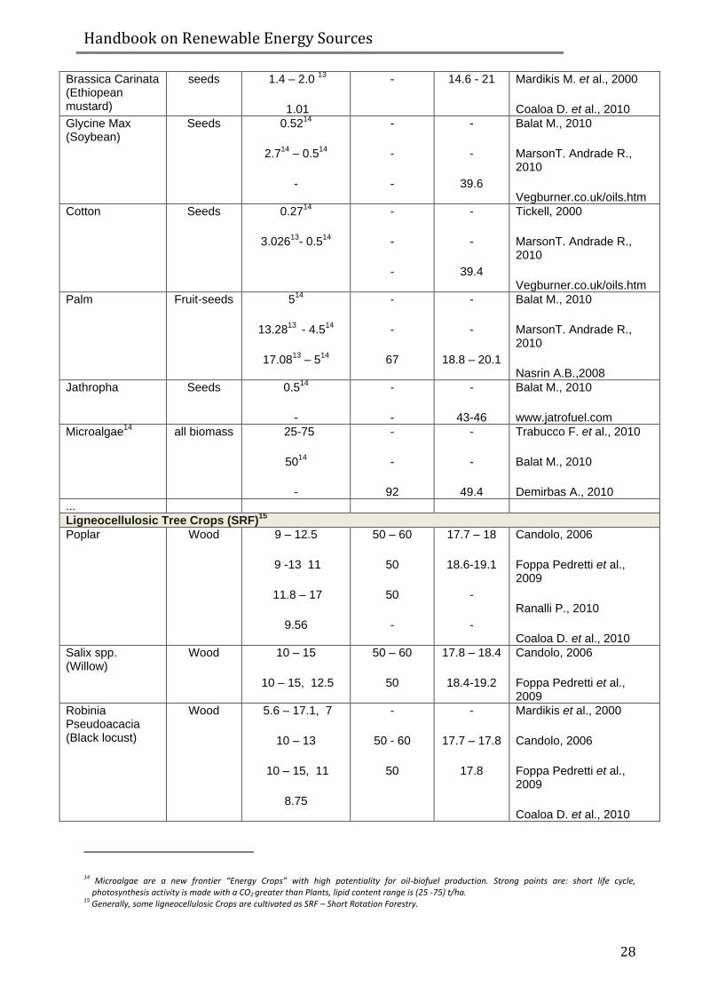
Ligneocellulosic Tree Crops (SRF)15
Poplar Wood 9 – 12.5
9 -13 11
11.8 – 17
9.56
50 – 60
50
50
-
17.7 – 18
18.6-19.1
-
-
Candolo, 2006
Foppa Pedretti et al., 2009
Ranalli P., 2010
Coaloa D. et al., 2010
Salix spp. (Willow)
Wood
10 – 15
10 – 15, 12.5
50 – 60
50
17.8 – 18.4
18.4-19.2
Candolo, 2006
Foppa Pedretti et al., 2009
Robinia Pseudoacacia (Black locust)
Wood 5.6 – 17.1, 7
10 – 13
10 – 15, 11
8.75
-
50 - 60
50
-
17.7 – 17.8
17.8
Mardikis et al., 2000
Candolo, 2006
Foppa Pedretti et al., 2009
Coaloa D. et al., 2010
14 Microalgae are a new frontier “Energy Crops” with high potentiality for oil-biofuel production. Strong points are: short life cycle, photosynthesis activity is made with a CO2 greater than Plants, lipid content range is (25 -75) t/ha.
15 Generally, some ligneocellulosic Crops are cultivated as SRF – Short Rotation Forestry.

Handbook on Renewable Energy Sources
29
Eucalyptus spp. (Eucalyptus)
Wood 8 – 9
12
50
50
16 - 1916
18.6
Mardikis et al., 2000
Foppa Pedretti et al., 2009
Coniferous coppice
Wood 35 - 60 40 - 50 18.8-19.8 Foppa Pedretti et al., 2009
Deciduous Coppice
Wood 36 -60 40 -50 18.5-19.2
Foppa Pedretti et al., 2009
4.3.2 Biomass potential by residuals and wastes
Residuals from Agricultural sector
From the UE report about agricultural Residues evaluation, residues crops covers over 1% of
the total Farmed land (UAA)17 in EU15 and produce dry lignocellulosic residues (moisture
content <50%). These concern: common wheat (10,8% of UAA), durum wheat (2,9% of UAA),
barley (8,7% of UAA), maize (3,3% of UAA), sunflower (1,6% of UAA), rapeseed (2,8% of UAA),
olive trees (2,8% of UAA) and vines (2,7% of UAA) and other crops (Siemons R., 2004).
The amount of residues produced by a specific crop (typically called residue-to-product ratio)
can vary significantly according to the agricultural practices, to the variety considered or to the
local climatic conditions. Therefore, estimates of the residue-to product ratio should be as much
specific as possible according the studied area. However, since these data are rarely available
at local scale, it is possible to refer to studies published in the scientific or sectorial literature.
The technical potential of these crop residues is estimated by multiplying the cultivated areas
by the agricultural production for each crop in each country taking in consideration each
average production value and the residue ratios or residue yields (in dry tonnes/ha) derived
from literature.
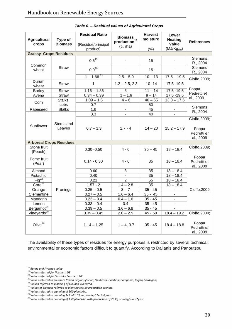
An overview of residuals production of agricultural crops are summarised in Table 8, in
according to different sources.
16 The range of calorific value is depending from part of plant more used: steam with or without leaves.
17 UAA – Utilized Agricultural Area.
http://epp.eurostat.ec.europa.eu/statistics_explained/index.php/Crop_production_statistics_at_regional_level
Handbook on Renewable Energy Sources
30
Table 6. – Residual values of Agricultural Crops
Agricultural crops
Type of Biomass
Residual Ratio
(Residue/principal product)
Biomass production
18
(tdm/ha)
Harvest moisture
(%)
Lower Heating Value
(MJ/Kgdm)
References
Grassy Crops Residues
Common wheat
Straw
0.519
- 15 - Siemons R., 2004
0.920
- 15 - Siemons R., 2004
1 – 1.66 21
2.5 – 5.0 10 – 13 17.5 – 19.5 Cioffo,2009;
Foppa Pedretti et al., 2009.
Durum wheat
Straw 1 1.2 – 2.5, 2.3 10 -14 17.5 -19.5
Barley Straw 1.16 – 1.36 3 11 – 14 17.5 -19.5
Avena Straw 0.34 – 0.39 1 – 1.6 9 – 14 17.5 -19.5
Corn Stalks, cobs
1.09 – 1.5 4 – 6 40 – 65 13.8 – 17.6
0.7 - 50 - Siemons R., 2004
Rapeseed Stalks 1.6 - 45 -
Sunflower Stems and
Leaves
3.3 - 40 -
0.7 – 1.3 1.7 - 4 14 – 20 15.2 – 17.9
Cioffo,2009;
Foppa Pedretti et al., 2009
Arboreal Crops Residues
Stone fruit (Peach)
Prunings
0.30 -0.50 4 - 6 35 – 45 18 – 18.4 Cioffo,2009;
Foppa Pedretti et al., 2009
Pome fruit (Pear)
0.14 - 0.30 4 - 6 35 18 – 18.4
Almond 0.60 3 35 18 – 18.4
Cioffo,2009
Pistachio 0.40 - 35 18 – 18.4
Fig22
0.21 2 55 18 – 18.4
Core23
1.57 - 2 1.4 – 2.8 35 18 – 18.4
Orange 0.25 – 0.5 3 – 7 35 - 45 -
Clementine 0.27 – 0.5 1.6 – 6.4 35 - 45 -
Mandarin 0.23 – 0.4 0.4 – 1.6 35 - 45 -
Lemon 0.33 – 0.4 0.4 35 - 45 -
Bergamot24
0.39 – 0.5 3.6 – 6.8 35 - 45 -
Vineyards25
0.39 – 0.45 2.0 – 2.5 45 - 50 18.4 – 19.2 Cioffo,2009;
Foppa Pedretti et al., 2009
Olive26
1.14 – 1.25 1 – 4, 3.7 35 - 45 18.4 – 18.8
The availability of these types of residues for energy purposes is restricted by several technical,
environmental or economic factors difficult to quantify. According to Dalianis and Panoutsou
18 Range and Average value
19 Values referred for Northern UE
20 Values referred for Central – Southern UE
21 Values referred to Southern Italian Regions (Sicilia, Basilicata, Calabria, Campania, Puglia, Sardegna)
22 Valued referred to planning of 6x6 and 10x10/ha.
23 Values of biomass referred to planting 5x5 by production pruning.
24 Values referred to planning of 500 plants/ha.
25 Values referred to planning 2x1 with “Spur pruning” Techniques
26 Values referred to planning of 150 plants/ha with production of 25 Kg pruning/plant*year.

Handbook on Renewable Energy Sources
31
(1995) from the total agricultural residues produced in EU15, 48% are exploited in non-energy
(e.g. animal feeding) or traditional energy applications and a further 40-45% cannot be exploited
for various technical and/or economical reasons (Siemons R., 2004).
In according to that, data reported by Cioffo highlight that in southern Italy, the straw residual
use as energy product is to exclude, because it's destinated to the zootechnical sector or land
filled for agronomic purposes. Pruning wood seems to have a discrete success as energy
product: statistic data confirm that 31% of wood pruning yearly collected is used for energy
purpose (Cioffo, 2009).
Residuals from Zootechnical sector
The average volume of manure and slurry largely differs from one species of animal to another
and mainly depends on their age and live weight. However, mean values have been developed
by various researchers in order to assist in the planning, design and operation of manure
collection, storage and pre-treatment and utilisation systems for livestock enterprises. In this
analysis, the ASAE standard coefficients, presented in Table 9 in according with other value
presented in the literature are adopted. The values represent fresh manure and slurry. Having in
mind the possibilities of collection and energy use of the manure (in view of keeping animals
outdoors, or in small farms), only the 50% can be considered available for energy production.
Table 7. – Coefficient of wastes (manure and slurry) for animal category
Animal category
Live animal mass
(kg)
Total fresh
manure (kgm.)
27
Moisture (%)
TS
Total Solids
(% on Kgm.)
VS
Volatile Solids
(% on TS)
Biogas Production
(m3/tsv)
CH4 in Biogas
(%)
References
Bovine 640 50 – 55,
51 83 -88
86 11 – 15,12
80 – 85 300 – 450 60 –
65 ASAE
D384.1; F. Pedretti 2009,
Siemons R., 2004
Swine 60 5 – 6, 5.2
90 6 – 9, 8 75 – 90 450 – 550 60 –
65
Horse 500 20 – 24.5 23.6
85 14 – 15,
15 75 250 – 500
60 – 65
Broiler 1.6 - 3.5
0.52 -0.72
75 19 – 25,
23 75 300 – 500
60 – 65 ASAE
D384.1; F. Pedretti 2009,
Siemons R., 2004
Turkey 6 -15 0.48 -
1.2 74 19 95 – 98 300 – 500
60 – 65
Duck 6.5 -8 0.52 -0.64
74 49 33 300 – 500 60 –
65
Ovine 70 -80 5.6 – 6.4
- 22 -40 70 – 75 300 – 500 60 –
65
On the basis of assumptions and data estimated by Siemons, the availability of wet manure in
the EU (UE15+10+2) is about 14 Mtoe, which could be used for Methane production by
anaerobic digestion.
27 Fresh manure is referred for live weight animal indicated.

Handbook on Renewable Energy Sources
32
As reported in tab 9, the amount of wastes produced by a single unit is estimated according to
the species of the animals (cattle, hogs, chicken and horses). Moreover, it depends on their age
and on their function (e.g., milkers and calves will produce different amount of wastes). The
theoretical potential should be estimated after an analysis of the animal farm, livestock units and
farming practices. However, in most cases, this survey is uneasy or too expensive to be carried
out.
Residuals from Forestal Sector
Forestry by-products are all those biomass that originate in the forests during forestry activities.
They include bark and wood chips made from tops and branches, as well as logs and chips
made from thinnings. As soon as these by-products are subjected to a manufacturing process
(like, e.g., briquetting or pelletizing of saw dust and wood shavings) they are considered
industrial products.
Table 8. - Residuals value of Forestal sector.
Forestal wood
categories
Type of Biomass
Biomass production
28
(tdm/ha)
Harvest moisture
(%)
Lower Heating Value
(MJ/kgdm) References
Hardwood Forest
tops and branches
2 – 4 25 – 60, 40 18.5 – 19.2 F. Pedretti E.,
2009 Coniferous Forest
tops and branches
2 – 4 25 – 60, 40 18.8 – 19.8
Wood from river bank
Tops and branches
0.8 – 1.6 29
40 – 60 16 -18 Francescato,
2009.
Residuals and Wastes from Industrial Sector
Several analyses of industrial wastes around UE estimate that the industrial residues of the UE
countries (27) reach 13 Mtoe, (Siemons R., 2004).
Industrial residues include industrial waste wood from sawmills and timber mills (bark, sawdust,
wood chips, slabs and off-cuts). Also the wastes from paper and pulp mills (e.g. black liquor) are
included but the largest resource of industrial residues is generated by the food industry. These
residues may consist of wet cellulosic material (e.g. beet root tails), fats (used cooking oils) and
proteins (i.e.: slaughter house waste). Not all the residues can be taken in consideration in this
section due to lack of data, but some of them are here reported.
28 Range and Average value
29 Range value is referred to “wet tons per 100 m linear meter”.

Handbook on Renewable Energy Sources
33
Table 9. – Residuals and wastes by Industrial sector
Industrial categories
Type of Biomass
Biomass production
(tdm)
Harvest humidity
(%)
Lower Heating Value
(MJ/kgdm)
References
Residues and wastes from Forestal-Industry
wood from sawmills
bark, sawdust,
wood chips, slabs, off-cuts
- 2 5 -60 18 – 21 F. Pedretti,
2009.
paper and pulp mills
black liquor - - - -
Residues and wastes from Zootecnical-Industry
Industrial categories
Type of Biomass
% Wastes on live weight
(%) (MJ/tdm) References
Bovine
Swine
Poultry
Ovine
slaughter house waste
7 – 9
12 – 14
23 -26
8-11
50 – 60 1.59 – 28.05 F. Pedretti,
2009.
Residues and wastes from Agro – Industry
Categories Biomass
type (Biomass/Primary Product) Ratio
t/ha (%) (MJ/Kgdm) References
Vegetables Hull, husk, pod, shell
- - 75 - 90 - F. Pedretti,
2009.
Peach Pit/stone 0.07 0.88 12-15 19.6 – 22 Cioffo, 2009
Almond Shell 0.73 3.65 < 15 19.6 - 22
Hazel Shell
0.50
0.50 – 0.55
0.70
0.77
< 15
12-15
18.4 – 19
16.9 – 17.8
Cioffo, 2009
F. Pedretti, 2009.
Pistachio Shell 0.60 0.3 < 15 19.6 - 22 Cioffo, 2009
Orange Peel, fruit
pieces 0.10
1.48 – 2
> 80 - Cioffo, 2009
Olive residues Cake after all oil extraction
0.22 – 0.28 1.32-2.8
12 - 20 17.6 – 18.4 Cioffo, 2009
Grape Wine Marc waste
0.25 – 0.30
0.15 – 0.21
1.2– 1.5
45 – 50
40 - 70
-
16.5 - 17.4
Cioffo, 2009
F. Pedretti, 2009.
Residuals and Wastes by Urban Sector
As announced in the Art. 2 of the UE Dir 1999/31/ CE, biodegradable waste (BMW) is defined
as the waste that is capable of undergoing anaerobic or aerobic decomposition, such as food
and garden waste, paper and paperboard. Synthetic organic materials, such as plastics, are
excluded from this definition, since they are not biodegradable. However, the focus is on
biomass residues that can contribute to a net reduction in carbon emissions.
To estimate all biodegradable fraction of urban waste is complicated because countries have
different collecting and management of wastes. Therefore, just a list of the principal classes of
waste has been reported (Tab. 12).
Table 10. Principal classes of Urban wastes

Handbook on Renewable Energy Sources
34
Categories Biomass
type (Biomass/BMW)
Ratio
Biomass production
(t/y)
Moisture
(%)
LHV
(MJ/kgdm)
References
Organic fraction of Urban BMW (households)
Organic matter
- - - - -
Organic fraction by commercial
services: restaurants,
schools, ecc...
Organic matter
- - - - -
Cooking oil exhausted
Oil - - - - -
Wood pruning by Urban streets
Wood branches
8 - 2530
80 -250 40 18 - 21 Foppa
Pedretti, 2009.
4.4 Calculation of Available Biomass
The studies and estimates on biomass resources – (especially the studies that consider all
types of biomass for relatively large geographical areas) generally have to face problems
connected reliability of data relating to existing residues, wastes, potential biomass by energy
crops and connected also to the definition of available resource, when limits – including
technical & economics – are uncertain.
To evaluate available biomass it's necessary to include into the model the different restrictions
(environmental, social and economic) that can limit its availability.
Once those available biomasses have been found, their uses could be only partially
sustainable.
The evaluation of "Sustainability Biomass Supply" – SBS - is possible just evaluating and
monitoring all key aspects of the bioenergy chain. A calculation of “Available Biomass Supply” –
ABS - from “Potential Biomass Supply” - PBS - is showed following.
In general, the amount of materials can be estimated using the following formula (Eq.1) that
returns the available tonnes of Biomass per year, taking in consideration the respective
biomass indexes above-mentioned. The aim is to estimate the amount of biomass (both like
primary product and residues) that can be collected over a certain region.
iiiiiiii econecolusecurrentlossRtPyielddedicatedcattleorAreaBiomass 1_11___
Eq. 1.
Where:
Area_or_cattle dedicatedi (ha/n°cattle): is the area or n° cattle involved i in the studied region;
Yieldi (t/ha): is the yield of crop or manure by cattle i in the studied region;
RtPi: is the residue-to-product ratio for crop/or manure by cattle i;
30 We assumed a percentage 8 – 25 % of residues wood/plant during thinning pruning.
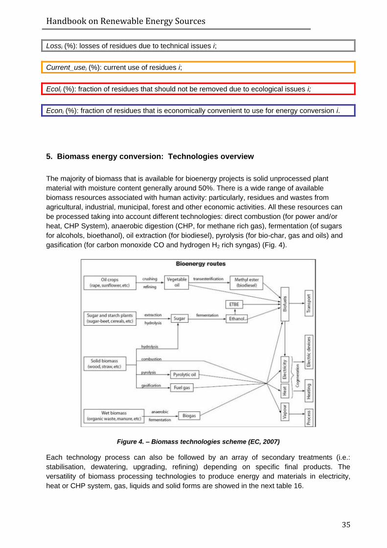
Handbook on Renewable Energy Sources
35
Lossi (%): losses of residues due to technical issues i;
Current_usei (%): current use of residues i;
Ecoli (%): fraction of residues that should not be removed due to ecological issues i;
Econi (%): fraction of residues that is economically convenient to use for energy conversion i.
5. Biomass energy conversion: Technologies overview
The majority of biomass that is available for bioenergy projects is solid unprocessed plant
material with moisture content generally around 50%. There is a wide range of available
biomass resources associated with human activity: particularly, residues and wastes from
agricultural, industrial, municipal, forest and other economic activities. All these resources can
be processed taking into account different technologies: direct combustion (for power and/or
heat, CHP System), anaerobic digestion (CHP, for methane rich gas), fermentation (of sugars
for alcohols, bioethanol), oil extraction (for biodiesel), pyrolysis (for bio-char, gas and oils) and
gasification (for carbon monoxide CO and hydrogen H2 rich syngas) (Fig. 4).
Figure 4. – Biomass technologies scheme (EC, 2007)
Each technology process can also be followed by an array of secondary treatments (i.e.:
stabilisation, dewatering, upgrading, refining) depending on specific final products. The
versatility of biomass processing technologies to produce energy and materials in electricity,
heat or CHP system, gas, liquids and solid forms are showed in the next table 16.

Handbook on Renewable Energy Sources
36
Table 11. - Overview of biomass Technologies (Crucible Carbon, 2008)
Technologies Energy and Biofuel Outputs
Heat Electricity Gas Liquid Solids
Direct Combustion
Anaerobic Digestion
Fermentation
Oil Extraction
Pyrolysis
Gasification
The selection of processing technologies depends on the nature and structure of the biomass
feedstocks and the desired project outputs. From the above table, it can be seen that direct
combustion or gasification of biomass are appropriate when heat and power are required.
Anaerobic digestion, fermentation and oil extraction are suitable with biomasses that have
easily extractable oils and sugars or high water contents. Only the thermal processing by
pyrolysis can provide the platform for all the forms of product above mentioned.
Many thermal technologies require the water content of biomass to be low (<15%) for proper
operation. For these technologies the energy cost of drying can represent a significant reduction
in process efficiency.
Therefore, it’s important to identify the biomass sources because some biomass species can
provide better quality of fuel or energy at lesser costs than others. For this purpose, energy-
from-biomass programmes are built around such species (Tasmeen A., 2009).
The energy density and physical properties of the biomass are critical factors for bioenergy
feedstock considerations and need to be understood in order to match a feedstock and
processing technology.
An overview about the capacity of generic biomass to be processed by using of available
technologies is shown below in table 17.
Table 12. - Chemical characterization of the different biomass sources (Crucible Carbon, 2008)
Fats, Oils Protein Sugars/Starch
Lignocellulose
Biomass Sources
Annual Crops Grassy Crops
Oil seed Crops
Perennial Crops
Grassy Crops
Oil Tree Crops
Ligneocellulosic Tree crops
Residues & Wastes
Green Waste
Animal Waste
Organic Fraction Urban Waste
Processing Technology
Direct Combustion
Anaerobic Digestion Cellulose only
Fermentation Cellulose Only
Oil Extraction
Pyrolysis
Gasification

Handbook on Renewable Energy Sources
37
A highly productive and scale able bioenergy industry must to make a full use of biomass
resources and constituents to recover maximum value. The overview shown in tab. 16
highlights that the lignocellulose is the constituent with the highest volume among the biomass,
therefore thermal processing and cellulose fermentation once tested could be one of the most
important sources for bioenergy world in next future; other specific processes (digestion, oil
extraction and fermentation) can be used as a primary processing treatment for biomass
sources with significant extractable non-lignocellulosic values (Crucible Carbon 2008). The
energy extracted depends not only on the available biomass, but also on the kind of energy
conversion technology used: using more efficient technologies produces more energy from the
same amount of available biomass. For this reason, in specific section about biomass
technologies has been discussed in Chapter 5.1 of the Biomass Handouts of the Project.
5.1 Integration between technologies: general aspects
A synthesis of the key factors for biomass processing technologies is presented below (Tab.
32). Thermal technologies are the least sensitive to the qualities of the feedstock and can
effectively process lignocellulosic materials. These technologies are the most size able and do
not require on grown purpose biomass. Technologies different from direct combustion are
significantly limited in scale for their dependence on specific and finite feedstocks. Technologies
that provide high volume and value opportunities are at present the less developed and are
candidates for future innovation.
Table 13. – Comparison between Technologies for the energy conversion of Biomass (Crucible Carbon, 2008).
Biomass processing technology
Possible Scale
31
Feedstock Flexibility
Conversion efficiency
32
Output Flexibility
Market Value of Product
Development Status
Direct Combustion Large High Low Low Low Established
Anaerobic Digestion Small Medium Medium Low Medium Established
Fermentation Medium33
Medium34
Medium Low High Established
Oil Extraction/Esterification
Small Low High Low High Established
Pyrolisis Large High Medium High Medium Early
Commercial
Gasification Large Medium Medium Medium35
Medium Early
commercial
The analysis highlights the strategic attractiveness of thermal processing to solid, liquid and gas
energy products, even if immediate term projects must be limited in scale.
31 Scale of possible industry is dependent on the scale of the available biomass resource. Those technologies able to use lignocellulosic biomass
are at an advantage. 32
Energy efficiency measures the amount of energy in the feedstock retained in the products. 33
De-polymerisation of cellulose to sugars will allow access to a larger biomass pool; however, this technology is not commercially established. 34
This may be higher if technologies that generate sugar feedstocks from cellulose become mature. 35
The direct products of gasification are low, but this is the basis to a vast array of fuel and chemical products via synthesis reactions.
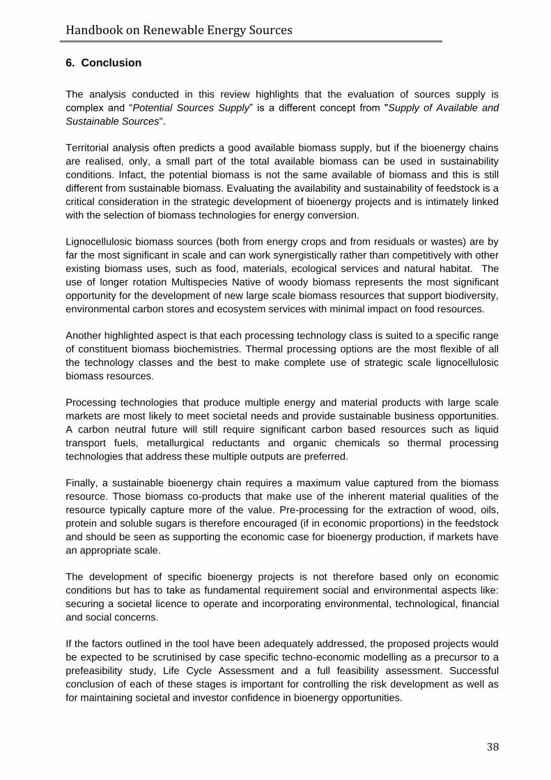
Handbook on Renewable Energy Sources
38
6. Conclusion
The analysis conducted in this review highlights that the evaluation of sources supply is
complex and “Potential Sources Supply” is a different concept from "Supply of Available and
Sustainable Sources".
Territorial analysis often predicts a good available biomass supply, but if the bioenergy chains
are realised, only, a small part of the total available biomass can be used in sustainability
conditions. Infact, the potential biomass is not the same available of biomass and this is still
different from sustainable biomass. Evaluating the availability and sustainability of feedstock is a
critical consideration in the strategic development of bioenergy projects and is intimately linked
with the selection of biomass technologies for energy conversion.
Lignocellulosic biomass sources (both from energy crops and from residuals or wastes) are by
far the most significant in scale and can work synergistically rather than competitively with other
existing biomass uses, such as food, materials, ecological services and natural habitat. The
use of longer rotation Multispecies Native of woody biomass represents the most significant
opportunity for the development of new large scale biomass resources that support biodiversity,
environmental carbon stores and ecosystem services with minimal impact on food resources.
Another highlighted aspect is that each processing technology class is suited to a specific range
of constituent biomass biochemistries. Thermal processing options are the most flexible of all
the technology classes and the best to make complete use of strategic scale lignocellulosic
biomass resources.
Processing technologies that produce multiple energy and material products with large scale
markets are most likely to meet societal needs and provide sustainable business opportunities.
A carbon neutral future will still require significant carbon based resources such as liquid
transport fuels, metallurgical reductants and organic chemicals so thermal processing
technologies that address these multiple outputs are preferred.
Finally, a sustainable bioenergy chain requires a maximum value captured from the biomass
resource. Those biomass co-products that make use of the inherent material qualities of the
resource typically capture more of the value. Pre-processing for the extraction of wood, oils,
protein and soluble sugars is therefore encouraged (if in economic proportions) in the feedstock
and should be seen as supporting the economic case for bioenergy production, if markets have
an appropriate scale.
The development of specific bioenergy projects is not therefore based only on economic
conditions but has to take as fundamental requirement social and environmental aspects like:
securing a societal licence to operate and incorporating environmental, technological, financial
and social concerns.
If the factors outlined in the tool have been adequately addressed, the proposed projects would
be expected to be scrutinised by case specific techno-economic modelling as a precursor to a
prefeasibility study, Life Cycle Assessment and a full feasibility assessment. Successful
conclusion of each of these stages is important for controlling the risk development as well as
for maintaining societal and investor confidence in bioenergy opportunities.

Handbook on Renewable Energy Sources
39
HIDRO ENERGY

Handbook on Renewable Energy Sources
40
1. INTRODUCTION 1.1 Basic definitions and processes
Hydroelectric power comes from water at work, water in motion. It can be seen as a form of solar energy, as the sun powers the hydrologic cycle which gives the earth its water. In the hydrologic cycle, atmospheric water reaches the earth’s surface as precipitation. Some of this water evaporates, but much of it either percolates into the soil or becomes surface runoff. Water from rain and melting snow eventually reaches ponds, lakes, reservoirs, or oceans where evaporation is constantly occurring.
Figure 1: Hydrologic cycle
Moisture percolating into the soil may become ground water (subsurface water), some of which also enters water bodies through springs or underground streams. Ground water may move upward through soil during dry periods and may return to the atmosphere by evaporation. Water vapour passes into the atmosphere by evaporation then circulates, condenses into clouds, and some returns to earth as precipitation. Thus, the water cycle is complete. Nature ensures that water is a renewable resource.
Small hydro is the largest contributor of electricity from renewable energy sources, both at European and world level. At world level, it is estimated that there is an installed capacity of 47.000 MW, with a potential - technical and economical - close to 180.000 MW.
Small scale Hydro Power (SHP) is mainly "run of river", i.e. not involving significant impounding of water and therefore not requiring the construction of large dams and reservoirs, though where these exist and can be utilised easily they do help. There is no general international consensus on the definition of SHP; the upper limit varies between 2.5 and 25 MW in different countries, but a value of 10 MW is becoming generally accepted and has also been accepted by ESHA (the European Small Hydro Association).
The definition for SHP as any hydro systems rated at 10 MW or less will therefore be used herein. SHP can be further subdivided into “mini hydro”, usually defined as those systems with capacity < 500kW, and “micro hydro” for systems with capacities < 100kW. Whichever size definition is used, SHP is one of the most environmentally benign forms of energy generation, based on the use of a non-polluting renewable resource, and requiring little interference with the surrounding environment.

Handbook on Renewable Energy Sources
41
It also has the capacity to make a significant impact on the replacement of fossil fuel, since unlike many other sources of renewable energy, SHP can generally produce some electricity at any time on demand (i.e. it needs no storage or backup systems), at least at times of the year when an adequate flow of water is available, and in many cases at a competitive cost with fossil fuel power stations.
1.2 Advantages of small-hydro
Small-scale hydropower is one of the most cost-effective and reliable energy technologies to be considered for providing clean electricity generation. In particular, the key advantages that small hydro has over wind, wave and solar power are:
A high efficiency (70 - 90%), by far the best of all energy technologies.
A high capacity factor (typically >50%), compared with 10% for solar and 30% for wind A high level of predictability, varying with annual rainfall patterns
Slow rate of change; the output power varies only gradually from day to day (not from minute to minute).
A good correlation with demand i.e. output is maximum in winter
It is a long-lasting and robust technology; systems can readily be engineered to last for 50 years or more.
It is also environmentally benign. Small hydro is in most cases “run-of-river”; in other words any dam or barrage is quite small, usually just a weir, and little or no water is stored. Therefore run-of-river installations do not have the same kinds of adverse effect on the local environment as large-scale hydro.

Handbook on Renewable Energy Sources
42
2. HYDROPOWER BASICS
2.1 Head and flow
The objective of a hydro power scheme is to convert the potential energy of a mass of water, flowing in a stream with a certain fall, into electric energy at the lower end of the scheme, where the powerhouse is located.
The vertical fall of the water, known as the “head”, is essential for hydropower generation; fast-flowing water on its own does not contain sufficient energy for useful power production except on a very large scale, such as offshore marine currents. Hence two quantities are required: a flow rate of water Q, and a head H. It is generally better to have more head than more flow, since this keeps the equipment smaller.
The Gross Head (H) is the maximum available vertical fall in the water, from the upstream level to the downstream level. The actual head seen by a turbine will be slightly less than the gross head due to losses incurred when transferring the water into and away from the machine. This reduced head is known as the Net Head.
The Flow Rate (Q) in the river is the volume of water passing per second, measured in m3/sec. For small schemes, the flow rate may also be expressed in litres/second where 1000 litres/sec is equal to 1 m3/sec.
According to the head, schemes can be classified in three categories:
High head: 100 m and above
Medium head: 30 - 100 m
Low head: 2 - 30 m.
These ranges are not rigid but are merely means of categorising sites.
Schemes can also be defined as
Run-of-river schemes
Schemes with the powerhouse located at the base of a dam
Schemes integrated on a canal or in a water supply pipe.
In general high-head sites are less expensive to develop than low-head sites, because for the same power output the flow through the turbine and required hydraulic structures will be smaller. In a river with a comparatively steep gradient over part of its course, the level difference can be utilised by diverting all or part of the flow and returning it to the river once it has passed through the turbine. The water can be brought from the intake directly to the turbine through a pressure pipe.
2.2 Power and Energy
Hydro-turbines convert water pressure into mechanical shaft power, which can be used to drive
an electricity generator, or other machinery. The power available is proportional to the product
of head and flow rate. The general formula for any hydro system’s power output is:
P = n ρ g Q H
where:
P is the mechanical power produced at the turbine shaft (Watts),

Handbook on Renewable Energy Sources
43
n is the hydraulic efficiency of the turbine,
ρ is the density of water (1000 kg/m3),
g is the acceleration due to gravity (9.81 m/s2),
Q is the volume flow rate passing through the turbine (m3/s),
H is the effective pressure head of water across the turbine (m).
The best turbines can have hydraulic efficiencies in the range 80 to over 90% (higher than all
other prime movers), although this will reduce with size. Micro-hydro systems (<100kW) tend to
be 60 to 80% efficient. If a typical water-to-wire efficiency for the whole system of 70% is
considered, then the above equation simplifies to:
P (kW) = 7 × Q (m3
/s) × H (m)
2.3 Main elements of a small hydropower scheme
Figure 2: Hydro-scheme components
Figure 2 illustrates a typical small hydro scheme on a medium or high head. The scheme can
be summarised as follows:
Water is taken from the river by diverting it through an intake at a weir.
In medium or high-head installations water may first be carried horizontally to the
forebay tank by a small canal or ‘leat’.
Before descending to the turbine, the water passes through a settling tank or ‘forebay’ in
which the water is slowed down sufficiently for suspended particles to settle out.
The forebay is usually protected by a rack of metal bars (a trash rack) which filters out
water-borne debris.
A pressure pipe, or ‘penstock’, conveys the water from the forebay to the turbine, which
is enclosed in the powerhouse together with the generator and control equipment.
After leaving the turbine, the water discharges down a ‘tailrace’ canal back into the river.

Handbook on Renewable Energy Sources
44
3. TECHNOLOGY
3.1 Overview
The main component of a small hydropower plant is the hydro turbine. All these turbines convert
the energy from falling water into rotating shaft power, but there is often confusion as to which
type of turbine should be used in different circumstances. The selection of the turbine depends
upon the site characteristics, principally the head and flow available, plus the desired running
speed of the generator and whether the turbine will be expected to operate in reduced flow
conditions.
There are two basic types of turbines, denoted as “impulse” and “reaction”. The “impulse
turbine” converts the potential energy of water into kinetic energy in a jet issuing from a nozzle
and projected onto the runner buckets or vanes. The “reaction turbine” uses the pressure, as
well as the velocity, of water to develop power. The runner is completely submerged and both
the pressure and the velocity decrease from inlet to outlet.
In contrast an impulse turbine runner operates in air, driven by a jet (or jets) of water. There are
3 main types of impulse turbine in use: the Pelton, Turgo and Crossflow (or Banki) turbines. The
two main types of reaction turbine are the propeller (with Kaplan variant) and Francis turbines. A
very rough classification of water turbines according to their type and the range of heads in
which they are applied is given in Table 1. These are approximate and depend on the precise
design of each manufacturer.
Table 1: Impulse and Reaction Turbines
Turbine Type Head Classification
High (>50m) Medium (10-50m) Low (<10m)
Impulse Pelton, Turgo, Multi-jet Pelton
Crossflow, Turgo, Multi-jet Pelton
Crossflow
Reaction
Francis (spiral case) Francis (open-flume),
Propeller, Kaplan
3.2 Types of turbines suitable for SHP
Most existing turbines may be grouped in three categories: • Kaplan and propeller turbines.
• Francis turbines.
• Pelton and other impulse turbines. Kaplan and propeller turbines are axial-flow reaction turbines, generally used for low heads (usually under 16 m). The Kaplan turbine has adjustable runner blades and may or may not have adjustable guide-vanes. If both runner blades and guide-vanes are adjustable it is described as 'double-regulated'. If the guide-vanes are fixed it is ‘single-regulated'. In the conventional version the Kaplan turbine has a scroll case (either in steel or reinforced cast concrete); the flow enters radially inward and makes a right-angle turn before entering the runner in an axial direction. When the runner has fixed blades the turbine is known as a propeller turbine. Propeller turbines can have mobile or fixed guide-vanes. Unregulated propeller turbines are only used when both flow and head remain practically constant. Bulb and tubular units are derived from propeller and Kaplan turbines, where the flow enters and exit with minor changes in direction. In the bulb turbine multiplier and generator are housed

Handbook on Renewable Energy Sources
45
within a bulb submerged in the flow. Tubular turbines permit several arrangements, namely right-angle drive, S ducts Straflo turbines, belt driven generators etc. Right-angle drives constitutes a very attractive solution but are only manufactured up to a maximum of 2 MW. Francis turbines are radial flow reaction turbines, with fixed runner blades and adjustable guide vanes, used for medium heads. The runner is composed of buckets formed of complex curves. A Francis turbine usually includes a cast iron or steel fabricated scroll casing to distribute the water around the entire perimeter of the runner, and several series of vanes to guide and regulate the flow of water into the runner. Figure 9 illustrates a schematic view of this type of turbine. Pelton turbines are Impulse turbines with single or multiple jets, each jet issuing through a nozzle with a needle valve to control the flow. They are used for medium and high heads. The axes of the nozzles are in the plane of the runner. Figure 10 illustrates the scheme of a vertical Pelton turbine and the axis of the nozzles placed on the same plan as the runner. Certain manufacturers have developed special types of machines, with a limited range of discharge and output, but which may be advantageous under certain circumstances. The cross-flow turbine, also sometimes called as the Ossberger turbine, after a company that has been making it for more than 50 years, or Michell turbine is used for a wide range of heads overlapping those of Kaplan, Francis and Pelton. It is specifically suitable for a high-flow, low-head stream. The Turgo turbine can operate under a head in the range of 30-300 m. Like the Pelton it is an impulse turbine, but its buckets are shaped differently and the jet of water strikes the plane of its runner at an angle of 20°. Water enters the runner through one side of the runner disk and emerges from the other. The higher runner speed of the Turgo, due to its smaller diameter compared to other types, makes direct coupling of turbine and generator more likely. A Turgo may prove appropriate at medium heads where a Francis turbine might otherwise be used. However, unlike in the Pelton, the water flowing through the runner produces an axial force, requiring the installation of a thrust bearing on its shaft.

Handbook on Renewable Energy Sources
46
PELTON
TURGO
OPEN-FLUME FRANCIS
SPIRAL-CASE FRANCIS
CROSSFLOW
PROPELLER
Figure 3: Schematics of principal turbine types
3.3 Turbine selection criteria
The type, geometry and dimensions of the turbine will be fundamentally conditioned by the

Handbook on Renewable Energy Sources
47
following criteria: • Net head • Range of discharges through the turbine • Rotational speed • Cavitation problems • Cost
Figure 4: Operating ranges of different types of turbines
Figure 4 presents the operating ranges of different turbine types as a function of the net head
and the discharge. The net head by itself constitutes the first criterion in the choice of the type of
turbine to install. Next table indicates the range of suitable net heads for the different types of
turbines.
Table 2: Range of heads
Types of turbine Range of head in meters
Kaplan and propeller 2 < H < 15
Francis 4 < H < 100
Pelton 30 < H < 1000
Cross-flow 1 < H < 150
Turgo 50 < H < 250
For the same net head, certain turbines are more difficult to manufacture than others and
consequently they are more expensive. For instance, for low heads, a propeller turbine is
cheaper than a Kaplan designed for the same rated discharge. In a medium head scheme, a
cross flow turbine will be cheaper than a Francis, whose runner is more complex, although its
efficiency is higher. Regarding discharge it must be remembered that turbines cannot operate
from zero flow to rated discharge.
3.4 Turbine efficiency

Handbook on Renewable Energy Sources
48
The efficiency of a turbine is defined as the ratio of power supplied by the turbine (mechanical
power transmitted by the turbine shaft) to the absorbed power (hydraulic power equivalent to
the measured discharge under the net head). To estimate the overall efficiency the turbine
efficiency must be multiplied by the efficiencies of the speed increaser (if used) and the
alternator.
As can be seen in figure 4, that shows the mean efficiency for several types of turbine, the
efficiency decreases rapidly below a certain percentage of the rated discharge. A turbine is
designed to operate at or near its best efficiency point, usually at 80 % of the maximum flow
rate, and as flow deviates from that particular discharge so does the turbine’s hydraulic
efficiency.
The range of discharges to be used, consequently the generated energy, varies if:
• the scheme has to supply electricity to a small network,
• the scheme has been designed for connection to a large distribution network.
In the first case a discharge must be selected which enables generation of electricity almost all
the year. In the second, the rated discharge should be selected so that the net revenue from the
sale of electricity is maximised.
Double regulated Kaplan and Pelton turbines can operate satisfactorily over a wide range of
flow - upwards from about one fifth of rated discharge. Single regulated Kaplans have
acceptable efficiency upward from one third and Francis turbines from one half of rated
discharge. Below 40 % of the rated discharge, Francis turbines may show instability resulting in
vibration or mechanical shock. Propeller turbines with fixed guide vanes and blades can operate
satisfactorily only over a very limited range close to their rated discharge. It should be noted that
with single-regulated propeller turbines the efficiency is generally better when it is the runner
that is adjustable.
Figure 5: Part-flow efficiencies
3.5 Control
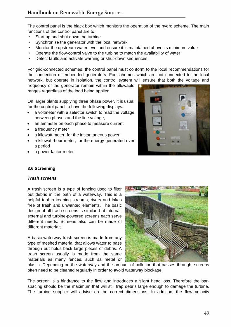
Handbook on Renewable Energy Sources
49
The control panel is the black box which monitors the operation of the hydro scheme. The main
functions of the control panel are to:
• Start up and shut down the turbine
• Synchronise the generator with the local network
• Monitor the upstream water level and ensure it is maintained above its minimum value
• Operate the flow-control valve to the turbine to match the availability of water
• Detect faults and activate warning or shut-down sequences.
For grid-connected schemes, the control panel must conform to the local recommendations for
the connection of embedded generators. For schemes which are not connected to the local
network, but operate in isolation, the control system will ensure that both the voltage and
frequency of the generator remain within the allowable
ranges regardless of the load being applied.
On larger plants supplying three phase power, it is usual
for the control panel to have the following displays:
a voltmeter with a selector switch to read the voltage
between phases and the line voltage,
an ammeter on each phase to measure current
a frequency meter
a kilowatt meter, for the instantaneous power
a kilowatt-hour meter, for the energy generated over
a period
a power factor meter
3.6 Screening Trash screens
A trash screen is a type of fencing used to filter
out debris in the path of a waterway. This is a
helpful tool in keeping streams, rivers and lakes
free of trash and unwanted elements. The basic
design of all trash screens is similar, but internal,
external and turbine-powered screens each serve
different needs. Screens also can be made of
different materials.
A basic waterway trash screen is made from any
type of meshed material that allows water to pass
through but holds back large pieces of debris. A
trash screen usually is made from the same
materials as many fences, such as metal or
plastic. Depending on the waterway and the amount of pollution that passes through, screens
often need to be cleaned regularly in order to avoid waterway blockage.
The screen is a hindrance to the flow and introduces a slight head loss. Therefore the bar-
spacing should be the maximum that will still trap debris large enough to damage the turbine.
The turbine supplier will advise on the correct dimensions. In addition, the flow velocity

Handbook on Renewable Energy Sources
50
approaching the screen should be relatively slow, preferably less than 0.3 m/sec and certainly
no greater than 0.5 m/sec.
Automatic cleaners
Manual raking is only viable for small schemes, or sites which are manned for other reasons.
There are now a range of automatic raking devices available to clean the screen and dispose of
the trapped debris. The most common types are:
A robotic rake: These come in a variety of designs, but usually involve one or more rakes
operated by a hydraulic ram. Some designs require only a single rake which can index along
the screen; otherwise two or more rakes can operate side by side. These systems are usually
very robust, partly because they can keep their drive mechanisms out of the water at all times.
Their main disadvantages are the visual presence of the equipment and the slightly greater
health and safety risk posed by unattended operation of the equipment.
A rake-and-chain cleaner, in which a bar is moved up the screen by a chain drive at each end.
The bar deposits the collected debris in a channel running the length of the screen. The channel
can be flushed clean by a water supply (pumped if necessary), washing the debris towards a
side spillway.
The grab-and-lift cleaner is a robust alternative to the robotic rake. A single set of ‘jaws’
indexes along the screen and lifts the material straight into a skip.
Coanda screens, applicable only for high and medium head schemes, require no raking
because they utilise the Coanda Effect to filter out and flush away debris and silt particles,
allowing only clean water into the intake system. Precisely positioned, finely spaced horizontal
stainless steel wires are built into a carefully profiled screen which is mounted on the
downstream face of the intake weir. Clean water is collected in a chamber below the screens,
which is connected directly to the turbine penstock.
(a) Rake and chain (b) Hydraulic arm
(c) Grab-and-Lift
(d) Coanda screen

Handbook on Renewable Energy Sources
51
Fish-screening
On rivers where there are important fisheries concerns, there are usually more stringent
screening requirements to ensure that fish will be deterred from the turbine intake and will be
diverted to a suitable by-wash. The precise fish-screening measures will be a matter for
negotiation, depending on the sensitivities of the site.
A number of innovative methods for excluding fish from intakes which avoid a physical screen
are being trialled. These include the use of electric currents, bubble curtains and sound waves
to guide the fish away from the intake. These methods offer significant advantages to the
operator by avoiding any obstruction to the flow.
4. RESOURCE ASSESSMENT 4.1 Introduction
The planning plays important role in the growth and development of hydropower. The amount of
achievable hydropower at any given site is a function of turbine head and the corresponding
flow rate. Thus, harnessing hydroenergy requires assessment of the water resource, which
depends upon the natural processes occurring locally and also the terrain characteristics.
Accurate and reliable assessment of water resources leads to successful planning. However,
reliable assessment of water resources has remained as constraint. This is particularly true for
the non-industrialized under-developed regions and this might be the one of the factors of
inadequate growth of hydropower in such regions.
Traditionally, the historic data of discharge corresponding to a fixed location are considered for
estimation of water resources, hence planners use such information. The Ministries of
Environment, the Hydrology and/or Environmental Agencies (National/regional/local) or other
similar organisations are usually a source for flow measures data in the most significant rivers
and streams of the European countries. The records can be used to assess stream flow at the
proposed site, as long as due allowance is made for the actual site location in relation to the
gauging station (upstream or downsteam).
But, in most of the cases the water availability records of past time are location specific. Due to
the complexity involved in the hydrological phenomenon, the future assessment based on past
location specific observed data poses doubts regarding the accuracy and reliability of
assessment. There may be several consequences of such inaccurate information of water
resource assessment:

Handbook on Renewable Energy Sources
52
1. the underestimation may be the chief cause of poor motivation for hydropower – even
the actual availability would have been encouraging;
2. the assessment based on the observation at selected location might miss some more
potential events at other locations, which might also results erroneous planning;
3. the collections of observed data from a large number of observatories covering wide
spatial extent are both costly and time consuming.
With the advent of modern computation tools such as geographical information system (GIS),
remote sensing and hydrological models, the constraints as discussed above can be addressed
more comprehensively. The realistic representations of: (i) existing terrain, (ii) complex
hydrological phenomena and (iii) varying climate are now possible through spatial tools and
modelling techniques. Thus, not only spatial but also temporal simulation of actual hydrology
vis-à-vis water availability of a region is now possible.
Hydrological models are simplified, conceptual representations of a part of the hydrologic cycle.
They are primarily used for hydrologic prediction and for understanding of hydrologic processes.
It is a powerful technique of hydrologic system investigation for both the research hydrologists
and the practicing water resources engineers. These models generally use mathematical and
statistical concepts to link certain inputs (for instance rainfall, temperature, etc.) to the model
output (for instance runoff).
It has become possible to integrate all the physical events leading to better simulation of
physical world using GIS and hydrological models. The advantages of these tools and models
are their capability to simulate water content in respect to discharge within miniature spatial
extent for three different flows, namely overland, surface and channel flows. The uses of
hydrological models have been increased due to their merit over traditional methods for water
resource assessment.
GIS and remote sensing tools have also been widely used for assessing hydropower potential
in recent times. The usefulness of GIS and remote sensing technologies are enhanced if
process based hydrological models could be integrated into it. Although there are number of
benefits of GIS integrated process based hydrological models, some limitations have also been
reported. The requirement of large volume of data concerning land use, soil and climate has
been one major limitation of hydrological modelling. Involvement of many sub-models and
associated considerations are also proved as limitations for some specific situation. Such
limitations could lead to prediction uncertainties of the model. However, uncertainties can be
minimized through standard procedure of calibration and validation.
4.2 National and regional levels
For national and regional resource assessment, the satellite images are used to develop GIS
database for identification of source, selection of site, environmental planning, digital terrain
model data (DTM), and transmission line network and ranking of the sites. Generally such
exercises for large scale resource assessments are carried out by a team comprising GIS,
hydrology, hydropower, etc. experts.
Geographic Information System (GIS) is a computer based information system used to digitally
represent and analyze the geographic features present on the earth’s surface. The methodology
for assessing the Hydro Power potential for a region can be done using the following methods.
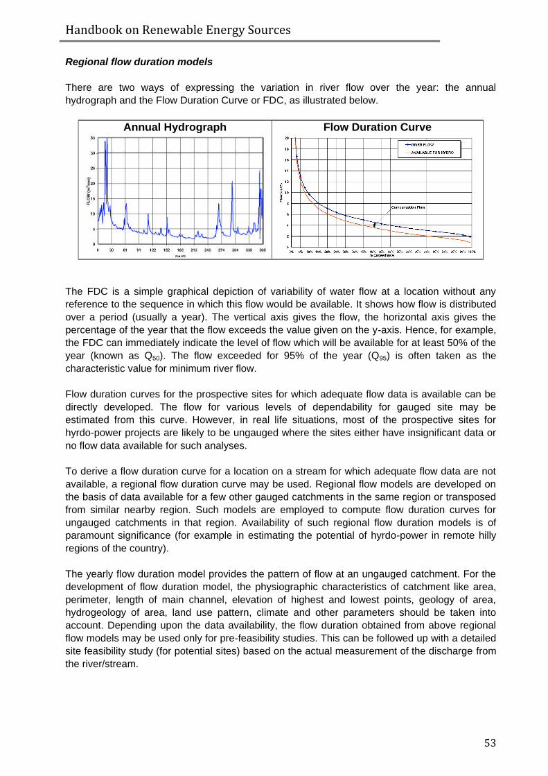
Handbook on Renewable Energy Sources
53
Regional flow duration models
There are two ways of expressing the variation in river flow over the year: the annual
hydrograph and the Flow Duration Curve or FDC, as illustrated below.
Annual Hydrograph
Flow Duration Curve
The FDC is a simple graphical depiction of variability of water flow at a location without any
reference to the sequence in which this flow would be available. It shows how flow is distributed
over a period (usually a year). The vertical axis gives the flow, the horizontal axis gives the
percentage of the year that the flow exceeds the value given on the y-axis. Hence, for example,
the FDC can immediately indicate the level of flow which will be available for at least 50% of the
year (known as Q50). The flow exceeded for 95% of the year (Q95) is often taken as the
characteristic value for minimum river flow.
Flow duration curves for the prospective sites for which adequate flow data is available can be
directly developed. The flow for various levels of dependability for gauged site may be
estimated from this curve. However, in real life situations, most of the prospective sites for
hyrdo-power projects are likely to be ungauged where the sites either have insignificant data or
no flow data available for such analyses.
To derive a flow duration curve for a location on a stream for which adequate flow data are not
available, a regional flow duration curve may be used. Regional flow models are developed on
the basis of data available for a few other gauged catchments in the same region or transposed
from similar nearby region. Such models are employed to compute flow duration curves for
ungauged catchments in that region. Availability of such regional flow duration models is of
paramount significance (for example in estimating the potential of hyrdo-power in remote hilly
regions of the country).
The yearly flow duration model provides the pattern of flow at an ungauged catchment. For the
development of flow duration model, the physiographic characteristics of catchment like area,
perimeter, length of main channel, elevation of highest and lowest points, geology of area,
hydrogeology of area, land use pattern, climate and other parameters should be taken into
account. Depending upon the data availability, the flow duration obtained from above regional
flow models may be used only for pre-feasibility studies. This can be followed up with a detailed
site feasibility study (for potential sites) based on the actual measurement of the discharge from
the river/stream.

Handbook on Renewable Energy Sources
54
Remote sensing data for catchment analysis
The remote sensing technology is an effective tool for the identification of suitable sites for
locating new hydropower projects especially in the inaccessible areas where the water recourse
potential is high. Remote Sensing data available in the near infrared region (0.8 um - 1.1 um)
provides clearly the contrast between land and water features and therefore is best suited for
mapping perennial streams. IRS-LISS III-Geocoded False Colour Composites (FCCs) data may
be used for identification of catchment boundary, drainage network; perennial streams, land-use
and vegetation cover for such assessments. The elevation contours and spot heights from
topographic maps can used to generate Digital Elevation model (DEM) of these catchments
using any of the several GIS software packages available – Manifold, ARC-INFO, MapInfo, etc.
For further analysis, the catchment boundary, drainage network and location of major habitation
can be overlaid on these DEMs.
Digital Terrain Models (DTMs)
Digital Terrain Models can be used for computation of slope, channel length, area of catchment,
head available for power generation and location of suitable sites for civil structures of small
hydro power projects such as diversion weir, feeder and head race channel, desilting tank,
forebay tank, power house building etc. The satellite imagery and GIS can further be used to
plan the suitable (optimum) pathways, profile analysis, the engineering design of towers and
wires and the cost estimation of transmission line network or feeder line to the nearest
substation.
4.3 Resource estimation at local levels (site specific)
The only resource needed for a small/micro hydro power plant is flowing water available at a
gradient. Planning for any small hydro plant begins with the (near to) accurate estimation of
head and flow available at the proposed site. In the following subsections various methods for
measuring the head and discharge available have been described in detail.
Measurement of head
Several methods exist for measurement of the available head. Some methods are more suitable
on low-head sites, but are too tedious and inaccurate on high-heads. It is always advisable to
take several separate measurements of the head at each site.
A further very important factor is that the gross head does not remain constant but varies with
the river flow. As the flow in the river increases, the tail-water level often rises faster than the
headwater level, thus reducing the total head available. Although this head variation is much
less than the variation in flow, it can significantly affect the power available, especially in low-
head schemes where even 0.5 metre is critical. To assess the available gross head accurately,
head water and tail-water levels need to be measured for the full range of river flows. Some of
the more common methods/techniques used for measurement of head are:
Dumpy levels and theodolite: The use of a dumpy level (or builder's level) is the conventional
method for measuring head and should
be used wherever time and funds allow.
These devices need precise calibrations
and should be used by experienced

Handbook on Renewable Energy Sources
55
operators. Dumpy levels are used with staffs to measure head in a series of stages. A dumpy
level is a device which allows the operator to take sight on a staff held by a colleague, knowing
that the line of sight is exactly horizontal. Stages are usually limited by the length of the staff to
a height change (usually of no more than 3 m). A clear unobstructed view is needed, so sites
with lots of vegetation are generally difficult to assess with this method. Dumpy levels only allow
a horizontal sight but theodolite can also measure vertical and horizontal angles, giving greater
versatility and allowing faster work.
Sighting meters: Hand-held sighting meters measures angle of inclination of a slope (these are
also called Inclinometers or Abney levels). They are small and compact, and sometimes include
a range finder which eliminates the problem of measuring linear distance. The error in
estimation is typically between 2 and 10 % depending upon the skill of the user.
Water-filled tube and pressure gauge: This is probably one of the simplest methods for
measuring the available head, but it does have certain shortcomings. The two main sources of
errors which must (and can) be avoided are ‘out of calibration’ gauges and air bubbles in the
hose. To avoid the first error, the gauge should be recalibrated both before and after each major
site survey. To avoid the second, a clear plastic tube should be used so that the bubbles can be
seen.
This method can be used on high-heads as well as low ones, but the choice of pressure gauge
depends on the head to be measured.
Water filled tube and rod: This method is well suited for low-head sites. It is cheap, reasonably
accurate and does not report many errors. Two or three separate attempts should be made to
ensure that the final results are consistent and reliable. In addition the results can also be cross-
checked with measurements made by another method, for instance by water filled hose and
pressure gauge.
Spirit level and plank: This method is similar in principle to the water filled tube and rod method.
In this method, a carpenter's spirit level placed on a reliably straight plank of wood and the
horizontal sighting is established. On gentle slopes this method tends to be very slow, but on
steep slopes it is useful.
Taking two readings at each step (by marking on end of the plank and turning it around) cancels
the errors. The error is generally around 2%.
Maps: As discussed in the earlier section on Regional assessments, large-scale maps are
useful for approximate head values, but are not always available or totally reliable. For high-
head sites (>100 m) 1:50,000 maps are useful for prefeasibility studies and are generally
available.
Altimeters: Altimeters are quite useful for high-head pre-feasibility studies. Surveying altimeters
generally give errors in the range of as less as 3% in 100 m. Atmospheric pressure variations
need to be allowed for, however, and this method cannot be generally recommended except for
approximate readings (pre-feasibility studies).
Measurement of flow
The purpose of a hydrology study is to predict the variation in the flow during the year. Since the
flow varies from day to day, a one-off measurement is of limited use. In absence of any

Handbook on Renewable Energy Sources
56
hydrological analysis, a long-term measuring system may be set up. Such a system is often
used to reinforce the hydrological approach and is also the most reliable way of determining
actual flow at a site. One-off measurements are useful to give a spot check on hydrological
predictions.
The flow measuring techniques discussed here are:
the weir method,
stage control method,
the salt gulp method,
the bucket method,
the float method,
current meters.
Measuring weirs: A flow measurement weir is a weir with a notch in it through which all the
water in the stream is made to flow/pass. The flow rate can be determined from the difference in
height between the upstream water level and the bottom of the notch. For reliable results, the
crest of the weir must be sharp and sediment must be prevented from accumulating behind the
weir.
Weirs can be made of concrete, metal or even timber and must always be oriented at right
angles to the stream flow. Location of the weir should be at a point where the stream is straight
and free from eddies. Upstream, the distance between the point of measurement and the crest
of the weir should be at least twice the maximum head to be measured. There should be no
obstructions to flow near the notch and the weir must be perfectly sealed against leakage.
Rectangular notch measuring weir: For short-term or dry-season measurements, temporary
measuring weirs (generally made of wood) are used and are staked into the bank and stream
bed. It is necessary to estimate the range of flows to be measured before the weir, to ensure
appropriate sizing of the weir notch. The use of permanent weirs may be a useful approach for
small streams, but for larger streams staging of weirs would be a better alternative.
‘Salt gulp’ method: The ‘salt gulp’ method of flow measurement is adapted from dilution gauging
methods with radioactive tracers used for rivers. It is somewhat easy to carry out, reasonably
accurate (error probability is less than 7%), and reliable for a wide range of stream types. It
gives better results the more turbulent the stream. Using this approach, a spot check of stream
flow can be taken in less than 10 minutes with very little equipment.
A bucket of heavily salted water is poured into the stream. The cloud of salty water in the
stream starts to spread out while travelling downstream. After some distance downstream it will
have filled the width of the stream. The cloud will have a leading part which is weak in salt, a
middle part which is strong in salt and a lagging part which is weak again. The saltiness
(salinity) of the water can be measured with an electrical conductivity meter. If the stream is
small, it will not dilute the salt very much, so the electrical conductivity of the cloud (which is
greater the saltier the water) will be high. Therefore low flows are indicated by high conductivity
and vice versa.
The flow rate is therefore inversely proportional to the degree of conductivity of the cloud. The
above phenomenon assumes that the cloud passes the probe in the same time in each case.
But the slower the flow, the longer the cloud takes to pass the probe. Thus flow is also inversely
Handbook on Renewable Energy Sources
57
proportional to the cloud-passing time. The equipments needed for ‘salt gulp’ flow measurement
are a bucket, table salt, a thermometer and a conductivity meter (range 0-1000 mS).
Bucket method: The bucket method is the simplest and fastest way of measuring flow in very
small streams. The entire flow is diverted into a bucket or barrel and the time for the container to
be filled is recorded. The flow rate is obtained simply by dividing the volume of the container by
the filling time. Flows of up to 20 l/s can be measured using a 200-litre oil barrel. Equipment
needed are a bucket/barrel and a stopwatch.
Float method: The principle of all velocity-area methods is that flow (Q) is equal to the average
velocity (V) over a uniform cross-sectional area (A). Mathematically it can be represented as:
Q = V × A
The cross-sectional profile of a stream bed is selected in such a way that it does not alter too
much over a certain distance/length of the stream (one can also take an average cross-section
for a known length of stream – provided the stream bed is not altering too much). A series of
floats, mostly pieces of wood, are then timed over a measured length of stream. A flow velocity
is obtained by averaging the results over a large number of trails. This velocity must then be
reduced by a correction factor which estimates the mean velocity as opposed to the surface
velocity. By multiplying averaged and corrected flow velocity, the volume flow rate can be
estimated.
Current meters: This is more accurate than the float method. A current meter consists of a shaft
with a propeller or revolving cups connected to the end. The propeller is free to rotate and the
speed of rotation is related to the stream velocity. A simple mechanical counter records the
number of revolutions of a propeller placed at a desired depth. By averaging readings taken
evenly throughout the cross section, an average speed of the stream can be obtained.
5. CRES METHOD FOR THE ASSESSMENT OF SMALL HYDRO POTENTIAL
5.1 General concept
The experimental potential as defined for small hydro plants includes the processed results
arising from on site measurements of flow rates at those water streams that are characterized
by exploitable water flows. These measurements have either been made for specific purposes
by national/regional/local bodies active in the field of water resources, or they have been
derived from the processing of older measurements realized by other involved organizations.
The data included in the experimental potential correspond to a “flow duration curve” in specific
water stream points. Based on these data from measurements and on the use of a water
streams model, which is derived from the processing of a Digital Elevation Model – DEM (as is
analytically described in the next section), the prediction of the flow elements of a water stream
is possible in every single point of the stream.
The later consists of the theoretical potential for small hydro plants and it is the basic input for
the calculations aiming at the estimation of the technically and economically exploitable
potential that shall follow. The theoretical potential data have been incorporated in the system’s

Handbook on Renewable Energy Sources
58
database and they offer the possibility for retrieval and representation of the available
information (flow duration curve prediction, topography and land uses elements) in specific
points, as well as for the more general overview of the potential in large areas of water streams
in the form of thematic representation maps.
The available potential is investigated through the processing of the above elements and after
imposing some constrains which have to do alternatively with:
- Legal and environmental aspects (land planning constraints, minimum remaining river flow),
- General techno-economic issues (minimum flow rate, net head, estimated power production,
penstock length/maximum distance from water inflow to the power station).
The output of this investigation is the determination of pairs of points (water inflow – power
station) that satisfy the above constraints. These pairs simulate hypothetical (under
investigation) projects, and they consist of the input data for the next steps aiming at the
evaluation of the technically and financially exploitable potential.
In order to estimate the technological potential the system simulates the choice and operation of
hypothetical water turbines with the use of algorithms in order to calculate the following (for
every hypothetical power plants consisting of the available potential):
- type of turbine and optimal installed capacity,
- energy produced,
- utilization factor of the turbine and of the available water flow rate,
while then follows an initial evaluation of the respective investment costs and financial feasibility
elements of the respective hypothetical project, through the calculation of
- the installation cost
- the O&M costs
- the energy production cost (expressed in € / kWh)
- some basic indexes of investment’s profitability (IRR, NPV).
As a result, the system suggests some parts of the water streams where small hydro power
plants of an optimal energy and financial efficiency could possibly be installed.
5.2 Description of the geographical system’s database
The system’s database consists of a central information reservoir where a number of data are
drawn either to be directly retrieved and simply processed or to be processed via more complex
procedures by calculation models. Depending on the information they include, the database’s
elements can be categorised as follows:
Theoretical potential data including data concerning the geographical distribution of the small
hydropower potential,
General geographic reference data consisted of the basic existing geographical layers of the
natural environment, of the infrastructures and of the land uses,
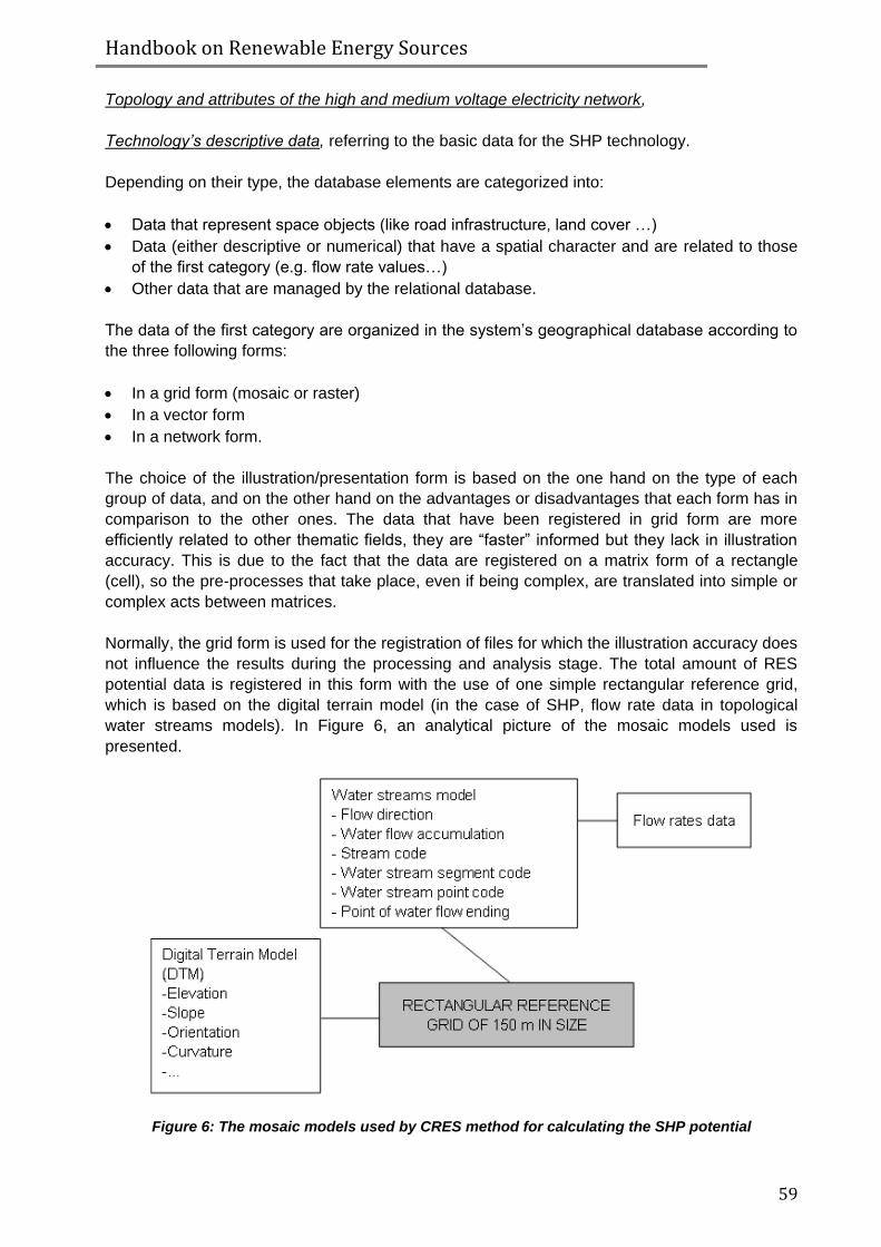
Handbook on Renewable Energy Sources
59
Topology and attributes of the high and medium voltage electricity network,
Technology’s descriptive data, referring to the basic data for the SHP technology.
Depending on their type, the database elements are categorized into:
Data that represent space objects (like road infrastructure, land cover …)
Data (either descriptive or numerical) that have a spatial character and are related to those
of the first category (e.g. flow rate values…)
Other data that are managed by the relational database.
The data of the first category are organized in the system’s geographical database according to
the three following forms:
In a grid form (mosaic or raster)
In a vector form
In a network form.
The choice of the illustration/presentation form is based on the one hand on the type of each
group of data, and on the other hand on the advantages or disadvantages that each form has in
comparison to the other ones. The data that have been registered in grid form are more
efficiently related to other thematic fields, they are “faster” informed but they lack in illustration
accuracy. This is due to the fact that the data are registered on a matrix form of a rectangle
(cell), so the pre-processes that take place, even if being complex, are translated into simple or
complex acts between matrices.
Normally, the grid form is used for the registration of files for which the illustration accuracy does
not influence the results during the processing and analysis stage. The total amount of RES
potential data is registered in this form with the use of one simple rectangular reference grid,
which is based on the digital terrain model (in the case of SHP, flow rate data in topological
water streams models). In Figure 6, an analytical picture of the mosaic models used is
presented.
Figure 6: The mosaic models used by CRES method for calculating the SHP potential

Handbook on Renewable Energy Sources
60
The vector form (vector) as well as the network one have been used in the case of files where
there is an important demand for accuracy in the information registration and illustration, so that
either a safe set of results (measurement of distance of hypothetical installations from roads or
energy grids) is assured, or there is a need for an accurate cartographic illustration. In Table 3
below the basic levels of the geographical database that are organised in a vector structure are
summarized.
Table 3:
THEMATIC LEVEL STRUCTURE USE
LAND COVERAGE
'CORINE' classification is followed
Vector, raster Environmental constraints control
for the installation of small
hydropower plants
INSTITUTIONALIZED LAND USES
- Natura protection areas
- Archeological sites
- General urban plans
- Residential Control Areas
- Industrial areas
Vector Environmental constraints control
for the installation of small
hydropower plants
SETTLEMENTS POINTS Vector Environmental constraints control
for the installation of small
hydropower plants
HYDROLOGICAL NETWORK Vector, network Registration of water streams flow
rates measurements
ROAD NETWORK Vector Calculation of distances and
extension works for possible
projects
HIGH AND MEDIUM VOLTAGE
ELECTRICITY NETWORK
Vector, network Connection parameters control,
connection cost calculation
ISOMETRIC ALTITUDE CURVES Vector Topography representation
ADMINISTRATIVE DIVISION
(districts)
Vector For local planning purposes
Some explanations necessary for the above variables are provided in the following:
Flow direction identifies the direction of the water flow in each rectangle. This means that, by
reading this information, one may be able to know to which one of the adjacent rectangles a
hypothetical water flow rate (e.g. precipitation) might be directed. The flow direction is
calculated by estimating the maximum head for every adjacent rectangle to the examined one.
The head is calculated as:
(Altitude difference between the rectangle being examined and the adjacent one)*100
Head =
Distance between the rectangles’ centres
This quantity is used as a basic input data for the flow accumulation evaluation.

Handbook on Renewable Energy Sources
61
Flow accumulation determines how many other cells a specific cell is being receiving water
from. Using the flow accumulation the tracing of the rivers in the area under investigation is
possible. This is done by selecting a certain value which will be the minimum value that can be
attributed to a cell in order this cell to belong to the water network of the area. The analysis
results are used in order to define the water stream class as well as to calculate the flow rate of
each water stream.
5.3 Methodological approach for calculating the exploitable potential of HPS
In the following, the specifications of the models that have been used for the design and
development of the software for the evaluation of the technical and economical exploitable small
hydro potential are analytically presented. As already mentioned, the models presented have
been incorporated in a software developed as libraries. These libraries are used by the
information system for the investigation of scenarios for the exploitation of small hydropower
potential.
Water streams data model
Water streams and the related to them information (hydrological catchment areas, flow rates,
etc) can be simulated using two different models.
The vectorial way of display, according to which a water stream is consisted of a series of linear
segments connected to each other by topological relations (segment class, segments
connection node, previous and next segment, etc). This way
All information concerning the stream under consideration (measured or calculated flow
rates data, terrain information such as the altitude, the orientation and the slope, etc) are
registered as segment or node elements being digitised from the respective maps.
The catchment areas at specific points of the water stream are polygons which are digitised
similarly to the water streams digitisation procedure. Any data of those catchment areas are
registered as those polygons’ data/elements.
The geographical accuracy of the registered data is considered as a comparative advantage of
the vectorial way of display, whereas the time consuming procedure of inserting and organising
the necessary data together with the ‘slowness’ as regards the implementation of analysis
calculations (especially in the case of calculation and exploitation of the catchment areas
elements as well as DTMs) are considered as basic disadvantages.
The second way of organising water streams elements consists of following the mosaic way of
display. According to this, the space is divided to normal unit segments (cells) and all available
information is registered in these cells. Following this model, a water stream is composed by a
number of such cell segments which are distinguished by their adjacent ones only based on the
fact that they consist parts of a stream (a value equal to 1 is appointed to those, while the others
are characterised by a 0 value).
As it is obvious, the above way does not guarantee the accurate geographical display of the
water stream elements. Furthermore, it does not easily realise the topological relations between
the stream’s elements (nodes, segments, catchment areas). On the other hand though, the
simplicity of the above described model can guarantee the unlimited capability of analysis, as
long of course as the two basic problems (accuracy, topology) have been overcome.
Handbook on Renewable Energy Sources
62
The methodology for the estimation of the technically and economically exploitable small hydro
potential is based on the continuous implementation of calculations as well as on the
implementation of algorithms taking into consideration among others the geographical and
topological data. Based on the initial consideration that the processing capability of the above
elements is more important than their geographical accuracy, the mosaic organisation model
has been chosen.
In the following paragraphs an analysis is provided of:
the DTM ‘s elements in relation to the water streams elements taking into account that water
streams data models are derived by the iterative processing of the DTM, as well as of the
implementation method of the whole water stream topological model.
5.4 Digital terrain model and water streams
The elements of the digital terrain model (DTM) are distinguished into: - Altitude data directly derived from measurement methods [altitude – z].
Morphological data arising from altitude data processing [slope – sl]36 [aspect - as] [profile curvature – prfcv]37 [planform curvature – plncv]38
Hydrographic network data derived through the processing of altitude data [flow direction – fd] [flow accumulation – fd]
The flow direction determines the direction (taking into consideration the 8 directions of the
adjacent cells) of maximum slope (figure 6) for a certain point. Accordingly, the flow
accumulation identifies the number of cells that are “directed” towards this specific cell. It could
be said that this parameter indirectly determines also the area of the catchment zone for every
single point where,
Catchment zone’s area = flow accumulation Χ cell area
It is obvious that all cells being attributed with a 0 flow accumulation value are characterized as
ridges, while cells with a large flow accumulation value are beds.
5.5 Topological water stream model
As shown in the previous chapter, the water stream data model is defined as a sum of points
which themselves consist a subset of the reference DTM. What is not defined using this model
though is the topological relations between every water stream’s elements. All it takes for these
topological relations to be expressed in a way is the determination of the following parameters
for every single stream:
The separate segments39 that compose the stream
36 First grade derivative of altitude
37 Second grade derivative of altitude
38 First grade derivative of the orientation
39 The segment is defined as the flow from one junction node to another
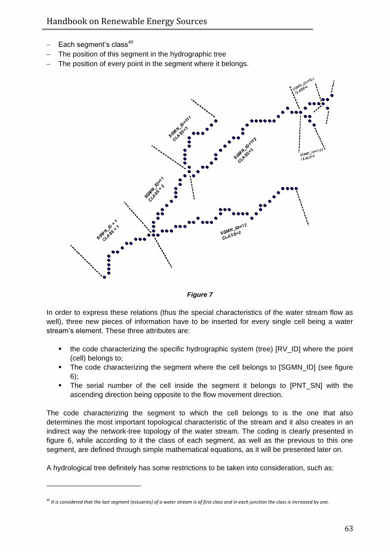
Handbook on Renewable Energy Sources
63
Each segment’s class40
The position of this segment in the hydrographic tree
The position of every point in the segment where it belongs.
Figure 7
In order to express these relations (thus the special characteristics of the water stream flow as
well), three new pieces of information have to be inserted for every single cell being a water
stream’s element. These three attributes are:
the code characterizing the specific hydrographic system (tree) [RV_ID] where the point
(cell) belongs to;
The code characterizing the segment where the cell belongs to [SGMN_ID] (see figure
6);
The serial number of the cell inside the segment it belongs to [PNT_SN] with the
ascending direction being opposite to the flow movement direction.
The code characterizing the segment to which the cell belongs to is the one that also
determines the most important topological characteristic of the stream and it also creates in an
indirect way the network-tree topology of the water stream. The coding is clearly presented in
figure 6, while according to it the class of each segment, as well as the previous to this one
segment, are defined through simple mathematical equations, as it will be presented later on.
A hydrological tree definitely has some restrictions to be taken into consideration, such as:
40 It is considered that the last segment (estuaries) of a water stream is of first class and in each junction the class is increased by one.
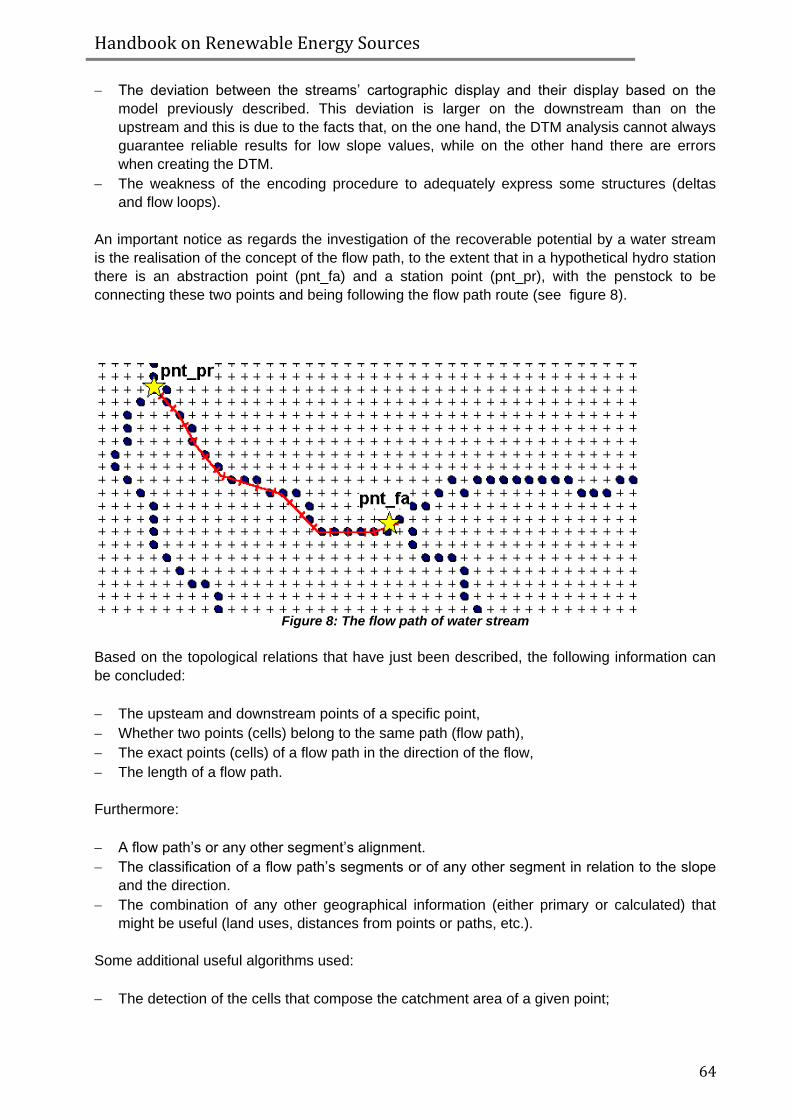
Handbook on Renewable Energy Sources
64
The deviation between the streams’ cartographic display and their display based on the
model previously described. This deviation is larger on the downstream than on the
upstream and this is due to the facts that, on the one hand, the DTM analysis cannot always
guarantee reliable results for low slope values, while on the other hand there are errors
when creating the DTM.
The weakness of the encoding procedure to adequately express some structures (deltas
and flow loops).
An important notice as regards the investigation of the recoverable potential by a water stream
is the realisation of the concept of the flow path, to the extent that in a hypothetical hydro station
there is an abstraction point (pnt_fa) and a station point (pnt_pr), with the penstock to be
connecting these two points and being following the flow path route (see figure 8).
Figure 8: The flow path of water stream
Based on the topological relations that have just been described, the following information can
be concluded:
The upsteam and downstream points of a specific point,
Whether two points (cells) belong to the same path (flow path),
The exact points (cells) of a flow path in the direction of the flow,
The length of a flow path.
Furthermore:
A flow path’s or any other segment’s alignment.
The classification of a flow path’s segments or of any other segment in relation to the slope
and the direction.
The combination of any other geographical information (either primary or calculated) that
might be useful (land uses, distances from points or paths, etc.).
Some additional useful algorithms used:
The detection of the cells that compose the catchment area of a given point;

Handbook on Renewable Energy Sources
65
The encoding of points of the water stream.
5.7 Energy production by Small Hydro plants
A potential site for the installation of a Small Hydro plant is defined by the water inflow site as
well as the site of construction of a hydro station along a water stream. The height difference
between these two sites is defined as the hydraulic (net) head (h).
The assessment of a potential small hydro site has to take into consideration the following
characteristics:
- The strong variation of the natural runoff of the water stream according to the seasonal
variation in a year, or even due to the difference between wet and dry hydrological years.
This specific characteristic is quite intense when it comes to small water streams.
- The water turbines variety. As mentioned previously, each type of available water turbines is
most suitable for a specific range of available nominal hydraulic net head (h) as well as of
nominal flow rate Qr, it has a different operation range, a different efficiency whose
maximum value depends on the water turbine’s nominal power, different size and cost.
Small hydros are also characterized by an additional specificity in comparison to large hydro, as
they usually do not possess any high capacity reservoir upstream, for financial reasons. It
should be mentioned that large hydros (unless those formed during the course of big rivers) are
equipped with a large dam which forms a high capacity reservoir. In this way, the natural runoff
of the water stream is disconnected by the flow rate that the water turbines can exploit, since
the main aim of large hydros is to cover the interconnected electricity network peaks.
Small hydros, due to their low power, cannot really contribute to the satisfaction of a large
interconnected electricity network peaks and this is the reason why the creation of a reservoir
consists of a disproportionate to the cost burden, with no respective investment benefit. These
are the reasons why a small hydro, even when formed through a water stream diversion, it
functions as a flow hydro, which means that its main role is to exploit the available natural run
off in the best possible way. This is also why the small hydro assessment analysis is completed
using the flow rate duration curve instead of the natural runoff time series, since the small hydro
has no reservoir but just a limited basin whose volume can provide some good conditions for
the water inflow in the conduit works and which corresponds to a few hours flow rate.
These are the reasons why a parametric analysis of the techno-economical characteristics of a
small hydro has to take place prior to the potential site assessment, as according to this
parametric analysis and based on a criterion, the optimum water turbines size (nominal flow rate
and nominal power) and the optimum number of water turbines to be installed will be selected.
The nominal flow rate of the water turbine Qr and the number of water turbines are form now on
considered as the variable parameters of the analysis methodology developed.
All the reasons mentioned above lead to the fact that the analysis of the technically and
financially exploitable hydroelectric potential is realised separately for each water stream. For
each water stream the system provides information about:
- the theoretical potential

Handbook on Renewable Energy Sources
66
- the available potential
- the technically and financially exploitable potential
as these are analysed in the following paragraphs. The necessary primary data that are inserted
in the system’s database include the water stream’s geographical data (topological
hydrographic tree) as well as the representative flow duration curve at a certain point or points
of the hydrographic tree.
THEORETICAL POTENTIAL
The theoretical potential is defined as the total potential energy that is available at pre-selected
nodes of the water stream. The data used are:
- Nodes of the water stream;
- The annual flow duration curve at one, at least, point of the water stream;
- Geographical data,
while the system calculates:
- the annual flow duration curve at each node of the water stream, according to the equal
surfaces law (continuity);
- the height difference between the nodes;
- the water’s potential energy at each branch of the water stream.
AVAILABLE POTENTIAL
During the overview of a water stream’s available potential, some availability filters are inserted
and these actually express some restrictions as regards the water’s exploitability. Other, non
energy, uses of water consist of an important availability parameter for a river (irrigation, water
supply, etc.). The system also provides for the user some useful information about the actors
involved in the use rights concerning the water, for each part (segment) of the water stream.
Some restrictions inserted by the user, represent rough rules regarding the accessibility, the
technical constraints and the viability for the exploitation of a water stream. Such restrictions
may be:
- the distance between the water stream’s branches (or nodes) and roads
- the distance between the water stream’s branches (or nodes) and MediumVoltage electricity
network.
- the minimum height difference
- the minimum mean annual flow rate
- geographical data (e.g. least penstock slope, distances, minimum-maximum altimetry, etc.)
- Land uses.
Taking into consideration the restrictions imposed, the system identifies those branches of the
water stream that satisfy them and thus are available for exploitation.
ANALYSIS PER WATER STREAM

Handbook on Renewable Energy Sources
67
In this section a techno-economical analysis of all hydro power station plants that could
potentially be installed at a specific water stream is realised. For every potential hydro power
station, the following parameters are estimated:
- the expected energy production on an annual basis
- the financial assessment indexes for the hydro station
The system proceeds with an evaluation of the possible hydro power plants according to their
energy efficiency and their financial feasibility and then it provides the following information:
- the most energy or financially efficient plants
- the most energy or financially efficient plants that could be simultaneously completed
The user is also given the opportunity to proceed with the analysis of a specific hydro station
which he might determine (specific water inflow points and water turbine site). The hydro power
plants classification is realised based on parametrically defined criteria, such as:
- the maximum energy production
- the least energy cost
- the maximum financial benefit (net present value)
- the maximun Return on Capital (Internal Rate of Return)
- General filters of allowed node pairs (introduction of user filters, as specified in the available
potential paragraph)
The user shall also be given the opportunity to set some rough restrictions concerning the
power plants under investigation (aiming at a lower number of examined power plants and thus
at the decrease of the computational time as well). That kind of restrictions might be:
- Maximum penstock length
- Minimum height difference
- Minimum mean annual flow rate
- Maximum number of turbines to be installed at each hydro station
- Geographical constraints (e.g. minimum penstock slope, distances, minimum-maximum
altimetry, etc.)
Based on the above constraints, the system can determine all the possible power plants for
which the “hydro power station analysis algorithm”, as described in the following chapter, is run.
HYDRO POWER STATION ANALYSIS ALGORITHM
The hydro power station analysis algorithm analyse in detail a hydro power station fro a specific
pair of nodes (water inflow – water turbine). The data used are:
- Water inflow point-Point of water turbine installation
- Geographical data
- Annual flow rate duration curve Ετήσια at the water inflow point
- Classification criterion

Handbook on Renewable Energy Sources
68
According to the methodology followed, the nominal flow rate of the water turbine for every pair
of nodes that optimizes the hydro power station according to the classification criterion is
estimated. The optimum nominal flow rate can be calculated making consecutive tests starting
from a reference value Qref. For every flow rate value, separate algorithms are run concerning
the hydro power station dimensioning, as well as the expected energy production on an annual
basis, the power plant cost calculation and the financial indexes calculation (cost of energy
production, IRR, NPV, etc.).
6. COMMISSIONING A FEASIBILITY STUDY
6.1 Preliminaries
Getting professional help
Any developer should seek independent professional advice before committing significant
finance to the design and construction of a small-scale hydro scheme.
The involvement of professionals in a small-scale hydro development can range from
preliminary site assessment, through the conducting of a feasibility study, to a full ‘turnkey’
service, handling every aspect of a development. In addition, there are several companies that
lease, develop and operate sites as a business activity, and can provide a full skills and finance
package.
Preliminary Site Assessment
An experienced professional should be able to indicate whether a site is worth considering
further, on the basis of an initial site visit and discussions with the developer and others.
Preliminary investigations of this type will typically require no more than 2-3 days’ work. A minor
investment at this stage could save much greater expense and potential complications later in
the development process.
The main issues that should be considered in a preliminary investigation are:
• The existence of a suitable waterfall or weir and a turbine site
• A consistent flow of water at a usable head
• The likely acceptability of diverting water to a turbine
• Suitable site access for construction equipment
• A nearby demand for electricity, or the prospect of a grid connection at reasonable cost
• The social and environmental impact on the local area
• Land ownership and/or the prospect of securing or leasing land for the scheme at a
reasonable cost
• An initial indication of design power and annual energy output.
The accuracy of the information may only be plus or minus 25%, however, this should be
sufficient for deciding whether to proceed to a more detailed feasibility study.
6.2 Feasibility

Handbook on Renewable Energy Sources
69
A feasibility study uses accurate data and looks closely at costs. It can take the project forward
from the initial idea to a final design that will support applications for project finance and the
necessary licenses. It is therefore wise always to employ a professional to conduct the
feasibility study and the detailed design work. The cost of a full feasibility study carried out by an
independent consultant depends on its scope and on the specific characteristics of the site, but
would typically be € 6,000-€ 12,000.
The following essential tasks should form components of a feasibility study:
1. Hydrological Survey - Typically, a hydrological survey would produce a flow duration
curve. This would be based on long-term records of rainfall and/or flow data, together
with a knowledge of the catchment geology and soil types. This long-term information
might be backed up by short-term flow measurements. The study should also include an
estimate of the required compensation flow.
2. System design - This would include a description of the overall project layout, including
a drawing showing the general arrangement of the site. The prominent aspects of the
works should be described in detail, covering:
Civil works (intake and weir, intake channel, penstock, turbine house, tailrace
channel, site access, construction details)
The generating equipment (turbine, gearbox, generator, control system)
Grid connection
3. System costing - A clear system costing would include a detailed estimate of the capital
costs of the project, subdivided into:
Civil costs
The cost of grid-connection
The cost of electro-mechanical equipment
Engineering and project management fees
Estimate of energy output and annual revenue - This would summarise the source data
(river flows, hydraulic losses, operating head, turbine efficiencies and methods of calculation)
and calculate the output of the scheme in terms of the maximum potential output power (in kW)
and the average annual energy yield (kWh/year) converted into annual revenue (€/year)
An additional task, which may form part of the main feasibility report but is often undertaken
separately, is the environmental assessment of the scheme.

Handbook on Renewable Energy Sources
70
WIND ENERGY

Handbook on Renewable Energy Sources
71
1. THE WIND IN THE WIND ENERGY
Winds are due to the fact that the Earth’s equatorial regions receive more solar radiation than
the Polar Regions, setting up large-scale convection currents in the atmosphere. According to
estimations from meteorologists, about 1% of the incoming solar radiation is converted into wind
energy, while the 1% of the daily wind energy input is nearly equivalent to the present world
daily energy consumption. This means that the global wind resource is very large, but also
widely distributed. Of course, more detailed assessments are required to quantify the resource
in particular areas.
The extraction of power from wind began very early in centuries, with wind powered ships, grain
mills and threshing machines. Only toward the beginning of this century high-speed wind
turbines for generation of electrical power have been developed. The term Wind Turbine is
widely used nowadays for a machine with rotating blades that converts the kinetic energy of
wind into useful power. Two basic categories of Wind Turbines exist: horizontal-axis wind
turbines (HAWT) and vertical-axis wind turbines (VAWT), depending on the orientation of the
rotor axis.

Handbook on Renewable Energy Sources
72
Figure 1: Wind turbine configurations
Nowadays, the major applications of wind energy involve electricity generation, with the wind
turbines operating in parallel with utility grid systems or, in more remote locations, in parallel
with fossil fuelled engines (hybrid systems). The gain from the exploitation of wind energy is
reduced fossil fuel consumption, as well as reduced overall electricity generation costs. Power
utilities have the flexibility to accept a contribution of about 20% from wind energy systems.
Wind-diesel systems can provide more than 50% fuel saving.
Producing electricity from the wind is a rather new industry (20 years ago there was actually no
commercial wind power in Europe). In some countries wind energy is already competitive with
fossil and nuclear power, even without accounting for the environmental benefits of wind power.
The cost of electricity from conventional power stations does not usually take full account of
their environmental impact (acid rain, oil slick clean up, the effects of climate change, etc.).
Wind energy production continues to improve in ways that reduce cost and improve efficiency.
Electricity from the wind costs about 5 to 8 € cents per kWh and is predicted to fall below 4 €
cents per kWh in the near future. Wind energy projects are simple and cheap to maintain. Land
rental fees paid to farmers provide valuable additional income in rural communities. Local
companies mostly undertake the construction work providing local employment, while long-term
jobs are created for maintenance work. Wind energy is a fast-growing worldwide industry. There
are approximately 60 manufacturers worldwide and most of them are European.
More than 10 major European banks and more than 20 European utilities have invested in wind
energy, as have individuals and companies. The wind industry is also a major employer. A
recent study by the Danish Wind Turbine Manufacturers Association concludes that the Danish
wind industry alone employs 8,500 Danes and has created a further 4,000 jobs outside
Denmark. The Danish wind industry is now a larger employer than the Danish fishing industry.
Total employment within the wind industry in Europe as a whole is estimated to exceed 20,000
jobs.
1.2 Rated power of a WT

Handbook on Renewable Energy Sources
73
A steady supply of reasonably strong wind is a necessary requirement for utilizing the power in
the wind. The maximum power that wind turbines (WTs) are designed to generate is called the
“rated power” and the wind speed at which it is achieved is the “rated wind speed”. This is
chosen to fit the local site wind regime, and is often about 1.5 times the site mean wind speed.
The Beaufort scale, a wind speed classification, gives a description of the effect of the wind. It
was initially designed for sailors and described the sea state, but has been modified to include
wind effects on land.
Figure 2: The power curve of a typical wind turbine
The power produced by the wind turbine increases from zero, below the cut-in wind speed
(usually around 5 m/s, but again varying with site), to the maximum at the rated wind speed
(see fig. 1.2). Above the rated wind speed, the wind turbine continues to produce the same
rated power but at lower efficiency, until shut down is initiated, when the wind speed becomes
dangerously high, i.e. above 25 to 30 m/s (gale force). This is the cut-out wind speed. The exact
specifications for identifying the energy capture of a WT depend on the distribution of wind
speed over the year at the site.
1.3 Power extraction by a wind turbine
Wind turbines use the kinetic energy of the wind flow. Their rotors reduce the wind velocity from
the undisturbed wind speed v1 far in front of the rotor to an air velocity v2 behind the rotor
(figure 1.3). This difference in velocity is a measure for the extracted kinetic energy that turns
the rotor and, at the opposite end of the drive train, the connected electrical generator. The
power extracted by a WT is given by:
P = ρ2cpηAv1³ (1.1)
with ρ the air density, cp the power coefficient, η the mechanical/electrical efficiency, and A the
rotor disk area.

Handbook on Renewable Energy Sources
74
Figure 3: Wind flow through a WT
In ideal conditions, the theoretical maximum of cp is 16/27=0.593 (known as the Betz limit) or, in
other words, a wind turbine can theoretically extract the 59.3% of the airflow energy content.
Under real conditions, the power coefficient reaches not more than 0.5, because it includes all
aerodynamic losses of the WT. In most of today's technical publications the cp value includes all
losses and is, in fact, the shortcut for cpη. The different power contents and extraction
potentials depending on the power coefficient and the efficiency of a WT are shown in figure 4.
In case that cp reaches its theoretical maximum, the wind velocity v2 behind the rotor is only the
1/3 of the velocity v1 in front of the rotor. Therefore, WTs situated in a wind farm produce less
energy due to the wind speed reduction caused by the WT in front of them. Increasing the
distance between the WTs can diminish the energy loss, because the surrounding wind field will
accelerate the wind behind a WT again. A properly designed wind farm can therefore have less
than 10% losses caused by mutual interference effects.
0
200
400
600
800
1000
0 2 4 6 8 10 12 14 16 18 20
Undisturbed Wind Speed, m/s
Po
we
r E
xtr
ac
tio
n, W
/m²
Stall control
Pitch control
P
Av cP
21
3
P
Av
2
16
271
3
P
Av
21
3
Figure 4: Power extraction per square meter of rotor disk area versus wind speed

Handbook on Renewable Energy Sources
75
The equation for the power extraction by a WT [eq. (1.1)] shows that the WT’s annual energy
generation depends on the wind speed distribution of the site, the air density, the rotor size and
the technical design. Especially, the tower height affects considerably the energy extraction,
because the wind speed increases with height above ground level. As regards the air density,
the air is generally less dense in warmer climates and also decreases with height, and its
density can range from around 0.9 to 1.4 kg/m3. This effect is very small in comparison to the
variation of wind speed.
1.4 Variability of the wind
The wind will vary over a few hours as a weather system passes. This variability in the wind
means that the electrical power generated is also always varying. This is unlike most
conventional power sources, where the fuel is usually kept constant. The fuel supply in wind
power generation is not a steady constant flow. The wind climate of a site describes this
variability statistically. Different places have different wind climates. The tropics have steady
moderate winds all year, temperate latitudes have much more variation in wind speed, in
particular more high wind speed occurrences.
As the wind power depends on the cube of the wind speed, it is evident that the average annual
power will vary from site to site. Sites with more high wind speeds will return more power. As a
simple example, two sites both with an average annual wind speed of 10 m/s are considered
(see fig. 5). As can be seen in the figure, the first site can have a total power in the wind over
the year of 1232.4W/m2, while the second one of 1739.5 W/m2. The importance of strong winds
is this way displayed, and thus the implications of wind climate on the economics of wind power
generation.
Figure 5: Differences in power production between two sites with the same average annual wind
speed
Additionally, the wind availability is not under control and, although it can be forecasted up to 36
hours ahead, the availability of power cannot be guaranteed at all times. In electrical power
terminology, the power produced by a single turbine is not "firm". Therefore, some form of
energy storage, such as batteries, or supply control, such as the electricity grid, is required. This
is a key factor in the economic viability of wind power. This apparent lack of firmness in the
supply has been used in the past as an argument against wind power.

Handbook on Renewable Energy Sources
76
However, the wind may be described in statistical terms. Then, the average annual amount of
power produced in a year is used to describe the installation. As demand on the grid is also
described in statistical terms, a proportion of wind power may be considered as "firm", provided
that only small amounts of wind-generated electricity are included. This is described by the
turbine's capacity or load factor. Further improvements in "firmness" can be achieved via
clusters of machines with large geographical separation. Then, the variation in wind availability
across this region is smoothed.
1.5 Variation with time
The wind is constantly fluctuating, and this is immediately apparent from an anemometer
recording the wind speed. If a long time series of wind speed is transformed to the frequency
domain as a power spectrum, then the time scale of the dominant energy in the wind can be
identified (figure 6). In temperate latitudes two main peaks are found, the largest at time scales
of a few days, the second with time scales of around 10 sec. The first is due to the passage of
large-scale weather systems, while the second one is associated with turbulence within the
flow.
Figure 6: A typical wind speed variance spectrum
Most significantly, the two peaks are separated by a gap from around 10 minutes to about 2
hours. Very little of the wind's energy is contained in this gap. This is very important since it
allows treating the two types of motion separately, with turbulence as a perturbation of the
large-scale flow. The mathematics of the solution are then much simplified, and the
instantaneous wind velocity can be expressed as the sum of the mean wind velocity and a
fluctuating component, namely: U(t) = Ū + U’(t).
The mean wind should be averaged over a period that sits within the spectral gap, typically 1
hour. This would then describe the steady state, thus the energy available to the wind turbine.
The fluctuating component also affects the power of the turbine but in a less direct manner,
since the turbine does not react to very rapid (i.e. less than a few minutes) variations in wind
speed or direction. This variation in wind speed with time can be visualised by describing the
structure of the wind as a series of eddies or three-dimensional whirls of all sizes carried along
by the mean flow.

Handbook on Renewable Energy Sources
77
Eddies are responsible for mixing the air and their action may be considered in a similar way to
molecular diffusion. As an eddy passes the measurement point, the wind speed takes the value
of that eddy for a period of time proportional to the eddy size; this is a “gust”. In most cases, the
wind variation over the turbine averages out and the extra loads are not significant. However, if
the eddy length scale is of the same order as the length scale of a turbine component, then the
variation in load may affect the whole component. A 3-second gust corresponds to an eddy size
of around 20 m (i.e. of similar size to the rotor blade), while a 15-second gust to 50m.
For this reason, the highest gust value of the relevant time scale is used to compute the
maximum permissible loads on the turbine or its components over the expected lifetime of the
turbine. This is expressed as a maximum wind speed and gust in a 50 year return period. Of
course, the wind speed may be exceeded in this period, but the margin on the loads will allow
for some overstepping. The calculation of loads is particularly important for flexible structures
such as turbines, which are more susceptible to wind induced damage than rigid structures, like
buildings.
2. WIND RESOURCE ASSESSMENT
2.1 Introduction
A wind turbine can be placed almost anywhere in a reasonably open ground. However, a wind
farm is a commercial development and must attempt to optimise its profitability. This is
important not only for the returns during the lifetime of the farm, but also for raising capital to
develop the site initially. For planning economically attractive wind energy projects, it is
necessary to have reliable knowledge of the wind conditions predominant at the area of
concern.
Due to temporal and financial reasons, long-term measuring periods are often left out of
consideration. As a substitute, mathematical methods can be used to predict wind speeds at
every location. The calculated wind conditions and energy production data can serve as a basis
for economical calculations. In addition, simulations of wind conditions can be used to correlate
wind measurements at a certain site to the wind conditions of neighbouring locations in order to
establish the wind regime for a whole area.
2.2 Determination of site conditions
As the wind speed can vary significantly between short distances, e.g. over some hundred
meters, procedures for evaluating the location of future wind turbine sites generally consider all
regional parameters which are likely to influence the wind conditions. Such parameters are:
obstacles in the near surrounding;

Handbook on Renewable Energy Sources
78
the environmental topography in the far region which is characterised by the vegetation, land
utilisation and buildings (ground roughness description);
the orography, like hills, may cause acceleration or deceleration effects on the air flow.
This information on the regional conditions is gained from topographical maps, as well as from
site visits to record the obstacles in the near surrounding. Satellite data of the environment were
also proven to be a valuable input. In areas where there are a large number of trees, indices of
vegetation deformation, such as the Griggs-Puttnam index for pine trees (see figure 7), have
been developed. These indices can give qualitative information on the speed and direction of
the prevailing wind, but they should be used with care since other factors may be important, or
the strong winds may only occur during the main growing season. Other indicators at the site
may include geomorphologic features, such as sand dunes.
Some wind resource information may already be available. Climatological mean wind data have
been presented in the form of isovent maps, which show lines of equal mean annual wind
speed taken from observational data records. The annual average available wind power at a
site could be estimated from these data. Some early assessment studies were performed with
these data, as little else was available. However it is not advisable to use isovent data for
anything other than a crude assessment of the overall wind resource of the region, since little
data from upland sites are usually available and the effect of the terrain is smoothed out.
Figure 7: Wind speed rating according to the Griggs-Puttnam index
There may be serious errors implicit in using these data as a means of assessing site in an
upland area, as the interpolation of wind speed across very steep terrain is not accurate, and
the wind power at a site may be seriously underestimated. In concluding, the data needed to
assess a site may be obtained from a number of sources, including:
archived meteorological data;
on site data;
data from numerical or physical modelling.
Some of the advantages and disadvantages of the various data are presented in Table 1 below.
An accurate estimation of the mean annual wind speed is required to calculate the mean annual
power expected from the site. Then, information on the distribution of wind speed over time is
required. To obtain this reliably, datasets spanning several years are required, but are usually
estimated from much shorter datasets with the aid of appropriate computer based models. After
that, the expected wind energy production can be established according to the wind turbine’s
power performance.

Handbook on Renewable Energy Sources
79
Table 1: Advantages and disadvantages of the various data for assessing potential wind turbine
sites
Advantages Disadvantages
Archived
Meteorological
Data
1. Long time series
2. Wide geographical spread
1. Rarely from representative sites
2. Measured at 10m, not at hub height
3. Difficult to interpolate in complex terrain
On Site Data 1. Data specific to real site
2. Data recorded at hub height
3. Data recording may be tailored for
specific information, e.g.
turbulence
1. Costly
2. Short time periods of data may be
unrepresentative
3. High data losses possible
4. Poor positioning of measurement equipment
give unrepresentative results
Modelling 1. Cheaper than on-site
measurements
2. Several locations may be
investigated in short time periods
3. Quick
1. May be unadvisedly applied
2. Model assumptions may be incorrect or
inadequate
3. Resolution may be too low
4. Scaling may be incorrect
2.3 Procedure
The most widely distributed procedure for the long-term prediction of wind speeds and energy
yields for single locations is the European Wind Atlas Model „WASP“ (see figure 8 for
illustration). A frequency distribution of wind speeds measured at a reference station for many
years is prepared in such a way that it can be transferred to other locations. The computer
model combines the detailed site description of the location for which wind potential has to be
predicted / compared with the modified frequency distribution of the reference station.

Handbook on Renewable Energy Sources
80
Figure 8: Required input for the application of the WASP code
The reference station might have a distance of up to 100 km away from the considered location.
In connection with the wind turbine’s power curve (electrical power as function of wind speed)
the expected energy production can be calculated for this location. A key design item of the
WASP code is that it uses polar co-ordinates with the origin at the site of interest. Thus, in the
area of the site the resolution is very high, with grid points as little as 2 m apart. The solution is
also most constrained there and so likely to have smaller errors.
WASP incorporates both physical models of the atmosphere and statistical descriptions of the
wind climate. The physical models used include:
Surface layer similarity - log law assumed.
Geostrophic drag law - estimation of surface wind based on Rossby number similarity.
Stability corrections - allowing for variation from neutral stability.
Roughness change - allowing for changes in land use across the area.
Shelter model - modelling the effect of a bluff body on the local flow.

Handbook on Renewable Energy Sources
81
Orography model - modelling the effect of flow speed-up over orography.
The wind climate is described statistically by a Weibull distribution derived for the reference
data. The derived Weibull distribution is designed to best fit the high-end of the wind speed.
This is justified by the fact that little power is generated at low wind speeds. The wind
distribution at hub height is then matched to the power curve of a turbine and the power
probability distribution can be computed. To gain the highest possible precision in the prediction
of the energy yield, only power curves measured by independent institutes should be applied. In
addition, new reference stations are built constantly to reduce the uncertainty of wind potential
predictions.
Depending on the complexity of the examined regions, different procedures are used to de-
termine wind conditions. Beside the above-mentioned computer code WASP, other procedures
exist like the meso-scale models. Generally speaking, these models require much
computational effort, but they make possible extensive three-dimensional fluid motion descrip-
tions, especially for complex mountainous terrain. A completely different way of resource
assessment incorporates wind speed measurements directly at the site of interest.
Such measurements, typically performed for the period of one year, can be correlated to the
whole neighbouring area or can be transformed to the hub height of certain wind turbine types
by utilising the flow simulations described above (often referred to as MCP-method: Measure,
Correlate, Predict). One way to incorporate site-specific wind measurements is to use the
recorded data as a reference station in the WASP code. This is especially useful if no other
reliable reference data are available, or in order to verify the predicted wind potential in complex
terrain.
3. WIND SPEED PROFILES & MEASUREMENTS
3.1 Wind speed profiles
The roughness of the earth surface diminishes the velocity of the wind. With growing height
above ground level, the roughness has less effect and the velocity of the wind increases.
Figure 9 provides an impression of a possible shape of such a wind velocity boundary layer. A
simple assumption for the distribution of wind speed over height (h) is the logarithmic profile:
vv h
z
*ln
0
where v is the wind speed at height h, v* is the friction velocity, κ the von Karman constant, and
z0 the roughness length.

Handbook on Renewable Energy Sources
82
0
20
40
60
80
100
120
140
0 2 4 6 8 10
Wind Speed / m/s
Heig
ht
/ m
Figure 9: Measured wind speed profile
Sometimes, a power law is used for the description of the wind profile like:
v2 = v1(h2/h1)
where: v2 is the wind speed at height h2 and v1 is the wind speed at height h1. Value α is
dependent on the roughness elements of the ground and is different from z0. More details
regarding the mean wind speed profiles as well as the flow of air inside the planetary boundary
layer are provided in the section related to meteorology and the wind structure.
3.2 Wind speed measurements
The assessment of the wind resource at a site ideally requires data with as long a time series as
possible at the location of the proposed turbines. In addition, an understanding of the turbulence
across the site and the rotor is useful for wind turbine design information. To achieve this would
require a fast sampling time and spatial distribution of the measurement points. In practice, time
and expense often rule out such a thorough investigation.
Wind speed measurements are the most critical measurements for wind resource assessment,
performance determination and prediction of the annual energy yield. In economic terms,
uncertainties translate directly into financial risk. There is no other branch where the importance
of uncertainties in wind speed measurements is as great as in wind energy. Due to lack of
experience, a lot of wind speed measurements have unacceptably high uncertainties, because
best practice codes in the selection of the anemometers, anemometer calibration, mounting of
the anemometers and selection of the measurement site were not applied.
An international anemometer calibration round robin comparison showed that uncertainties up
to more than plus/minus 3.5% occurred in the calibrations in different wind tunnels. This
translates into about 10% uncertainty in energy yield prediction. The wind tunnels accepted by
MEASNET (MEASurement NETwork) did not differ more than 0.5% from the reference wind
speed. MEASNET offers a Measurement Procedure for Cup Anemometer Calibrations,
especially developed for wind energy applications.

Handbook on Renewable Energy Sources
83
It is very important that each anemometer used for wind speed measurements is calibrated
individually in a wind tunnel. However, if the data collection is to continue for some time, it is
prudent to perform on-site calibrations using a reference anemometer. As important as the
anemometer calibration is the selection of the anemometers. Poor anemometer design causes
high uncertainties on wind speed measurements, even if they are individually calibrated in a
wind tunnel.
The reason is that in turbulent air under real atmospheric conditions, the anemometers behave
differently as in the wind tunnel. Investigations have shown that some anemometers are
extremely sensitive to flow inclinations, which under real conditions, occur even in flat terrain
due to turbulent flow. In complex terrain these effects are of major importance and lead to over-
or under-estimation of the real wind conditions. Only few anemometer designs avoid these
effects.
Another source of errors in wind speed measurements is the mounting of the anemometers.
Booms should be mounted so that the flow field disturbance due to their presence and that from
the mast is minimised. If a lightning protection is necessary, the same rule should be followed.
To avoid flow inclination effects, the accuracy of the horizontal mounting of the anemometers is
important as well. Best practice wind speed measurements over a period of at least one year
reduce the financial risk of a wind farm significantly as the uncertainties of proper wind speed
measurements are much lower than those from flow model predictions.
A representative position within the wind farm area has to be chosen. For large wind farms in
complex terrain, two or three representative met-mast positions should be chosen. At least one
measurement should be performed at hub height of the planned turbines because extrapolation
from a lower height to hub height causes additional uncertainties. If one of the met-masts is
positioned close to the wind farm area (like M1 or M2 in figure 10) it can be used as a wind
speed reference mast during the operation of the wind farm and for the determination of the
sectorial wind farm power performance.
Mref
M1
M1, M2: mast in undisturbed air flow
M2
Mref: reference mast in wind farm
Figure 10: Possible mast positions for wind speed measurements before and after the installation
of the wind farm
If energy production is guaranteed in a contract of a wind farm project, the parties should decide
on the position of the met-mast and an independent institute should do the wind speed

Handbook on Renewable Energy Sources
84
measurements and evaluations. To collect data from a specific site one or more masts are
erected near the proposed wind turbine sites. A selection of instruments is mounted on the mast
to record relevant data. All the measurements need to be logged and the data either stored on
tape at the site or downloaded automatically to a remote site e.g. the developer's office.
Measurements of wind speed and direction are obviously necessary, but other meteorological
elements, particularly temperature and pressure, should be also recorded for inter-site
comparison and completeness of the data set. The equipment used for these measurements
needs to be robust and reliable, since it will, in the main, be left unattended for long periods.
Measurements of wind speed and direction are required at least at two heights, namely at 10m
and hub height. If the data will be used to estimate the site’s surface roughness (z0), then at
least one more measurement height should be included.
Mean wind speed data are usually collected using cup anemometers, as they are reliable and
comparatively cheap. These cup anemometers often have much better response characteristics
than those used at meteorological observing sites. Wind direction is measured with a wind
vane. This provides a resolved horizontal wind speed and direction. If turbulence data for the
site are required, then 3-dimensional wind data are useful. These can be obtained using
propeller anemometers, which are less robust, or sonic anemometers, which are expensive.
These anemometers return information on both wind speed and direction. The data must be
sampled at high frequency, perhaps 20 Hz. This soon fills up data tapes and so cannot usually
be recorded continuously. The rotation of the cup or propeller anemometer is proportional to the
wind speed; this is measured either by a varying voltage or by a series of pulses. All rotational
anemometers have a threshold start up speed. This is usually between 0.5 m/s and 2.0 m/s.
The response of the instrument to changes in wind speed is described either by a distance
constant or a time constant. A distance constant is the length of the column of air that must
pass the head for the anemometer to respond to 63.2% of the step change and depends only
upon air density. The time constant is the time taken for the anemometer to repine to 63.2% of
the step change and varies inversely with wind speed. Consequently, cup anemometers tend to
over-estimate a decelerating wind, which is the so called "over run error".
Wind vanes are usually wire wound potentiometers. Typically maximum voltage is returned for
North relative to the instrument body, and minimum for around 357 deg. Thus a gap occurs
close to instrument North. Instrument errors of around + or –2 deg are usual, directions are
resolved to around 0.3 degs. The instruments must be carefully aligned and often this is the
greatest source of errors. The wind vane will be affected by the shadow of the mast, so it is
often orientated so that the mast is upwind for the least probable wind direction. A complete list
of the various types of anemometers used and their characteristics is provided in Table 2.
Table 2: Characteristics of the various types of anemometers
Anemometer Measurement Method Comments

Handbook on Renewable Energy Sources
85
Cup Wind speed related to
rotational speed of cups
Robust, reliable and inexpensive
Propeller Wind speed related to
rotational speed of propellers
Need to be aligned into wind, but
can give faster response than
cups. Less robust than cups.
Pressure
tubes
Wind speed proportional to
pressure increase in tubes
Need to be aligned into wind,
slow response.
Hot wire Wind speed related to cooling
of fine wire
Very sensitive and fast response,
but easy to damage, usually used
in wind tunnels.
Sonic Wind speed related to time of
flight of a sonic pulse between
transmitter and receiver
Measures wind speed and
direction and turbulent fluxes.
Difficult to calibrate.
It is important that data logging is reliable. For this to be so the logger must be well insulated
from the weather, particularly the rain. Many experiments suffer a huge loss of data due to a
variety of problems, including water ingress and power failures. Most prospective sites for wind
turbines tend to be in rather hostile environments, but there are many reliable data logging
systems on the market these days. It may be possible to collect data remotely, downloading
data via telephone line. This has the advantage that the data may be monitored regularly and
any instrument problems spotted quickly. In addition, other data may be corrupted. Careful
planning of the data collection stage is essential for the development of a wind power project.
3.3 Presentation of archived data
Daily weather information is usually freely available from meteorological services. However,
charges are usually made for archived data and consultancy services. Mean wind speed and
direction are often shown together on a wind rose, and figure 11 shows an example. The
dominant winds in a year for any meteorological station are then easily seen. The data can also
usually be subdivided to show the seasonal or monthly variation in mean winds. In general, in
northern Europe the dominant winds are from the southwest. However marked seasonal
variations in wind speed and direction can occur.

Handbook on Renewable Energy Sources
86
Figure 11: An example of a Wind Rose
In southern Europe, the wind regime is dominated by seasonal winds. The coldest winter
weather is most often associated with north and north-easterly winds. These variations can be
seen in station records of wind speed and temperature. Meteorological data from individual Met
stations can also be presented as a frequency table. The data from the Met station anemometer
are binned for each wind speed and wind direction range. These data are presented for the
whole year and for each month in the form of a table, such as the one that follows.
The mean wind speed and the most probable wind speed (usually somewhat lower) can then be
deduced by plotting the data as a probability distribution, as the one presented in the following
figure 12. Data can then be matched to a Weibull distribution and an estimate of the power
available can be computed. Developers can then define the criteria on which to base their
choice of turbine. There are long runs of data over a number of years from each individual Met
station, so the data forms a good statistical dataset and should not be affected by individual non
representative years.

Handbook on Renewable Energy Sources
87
Figure 12: Wind speed frequency distribution (measured data and calculated distributions)
3.4 Analysis of on-site data
Data may be partially analysed immediately or stored for later retrieval, depending upon the
facilities and ease of access to the site. Generally data are recorded every minute. Faster data
will allow more information on site turbulence characteristics to be assessed. The data must be
quality controlled to remove poor data, calibrate the readings and check for inconsistent data.
The remaining data are then analysed to give usually 10-minute mean wind speed averages
throughout the day, each day preferably for around a year, since this should include all
seasonal variations.
Some studies suggest that a minimum of 8 months data is required to ensure adequate
estimation of the annual wind resource. Other researchers have suggested that the winter wind
resource is most important as it coincides with the peak electricity demand. The data can then
be sorted into ranges or "bins" of wind speed, either for each wind direction or as a total. The
number of measurements falling into each bin is then counted and the binned data plotted as a
fraction of the total number of readings to give a frequency distribution.
From these data the mean wind speed and the most probable wind speed can be identified. A
distribution of the power in the wind (proportional to the cube of the wind speed) can be
obtained. The data may also be shown as the probability of a wind speed greater than a specific
wind speed, usually zero, u>0. These data can usually be matched to a two parameter Weibull
distribution, with the two parameters k and c derived using techniques such as methods of
moments, least squares fit and various others. More precisely, the two-parameter Weibull
distribution has been found to fit much wind data with acceptable accuracy. It is expressed as:
kk
cU
cU
ck
Up exp)(1
(3.1)

Handbook on Renewable Energy Sources
88
where p(U) is the probability density distribution of the mean wind speed U, c is the scale
parameter (with units of speed), and k is the shape parameter (dimensionless).
When k=2 the distribution reduces to a Rayleigh distribution, while if k=1 an exponential
distribution is found. These are special cases of the Weibull distribution (see figure 3.4). In
much of Northern Europe the k factors are close to 2. Integrating the first moment of eq. (3.1), it
is found that the scale factor c is closely related to the mean wind speed for the site, since:
k
cU1
1 (3.2)
where Γ(•) is the complete gamma function. Similarly,
kn
cU nn 1 , and so:
k
cU3
133 (3.3)
Then, the available power density E (in Watts/m2) is obtained as:
k
cE3
12
1 3 (3.4)
while the shape factor k is related to the variance of the wind σ2 by
kk
c1
12
1 222 (3.5)
On the other hand, it is very important to know that the data collected are representative, i.e.
that the year is not especially windy or calm. To be sure of this around 10 years’ data are
needed. Obviously this is not practical for one site. It is however possible to compare the site
data with met data from a nearby site and perform some type of measure-correlate-predict
(MCP) methodology to extend the site dataset effectively to 10 years.
There are a number of MCP methods available, such as:
1. Matching - deriving Weibull parameters from the measurement site and the reference site
and correlating them for the measurement period and then applying the correction to the
rest of the reference data.
2. Computing the wind speed factor between the site and the reference location, during the
measurement period and for each of the wind direction bins.
3. Fitting continuous functions to all of the data over the measurement period and applying it to
the rest of the reference data.
Once a long-term frequency distribution has been constructed the power curve of a turbine can
be matched with the wind data to give a frequency distribution of power production. This
equates to the expected annual power production at the site. The data can of course be
checked against a number of different turbines types and configurations to optimise the results.
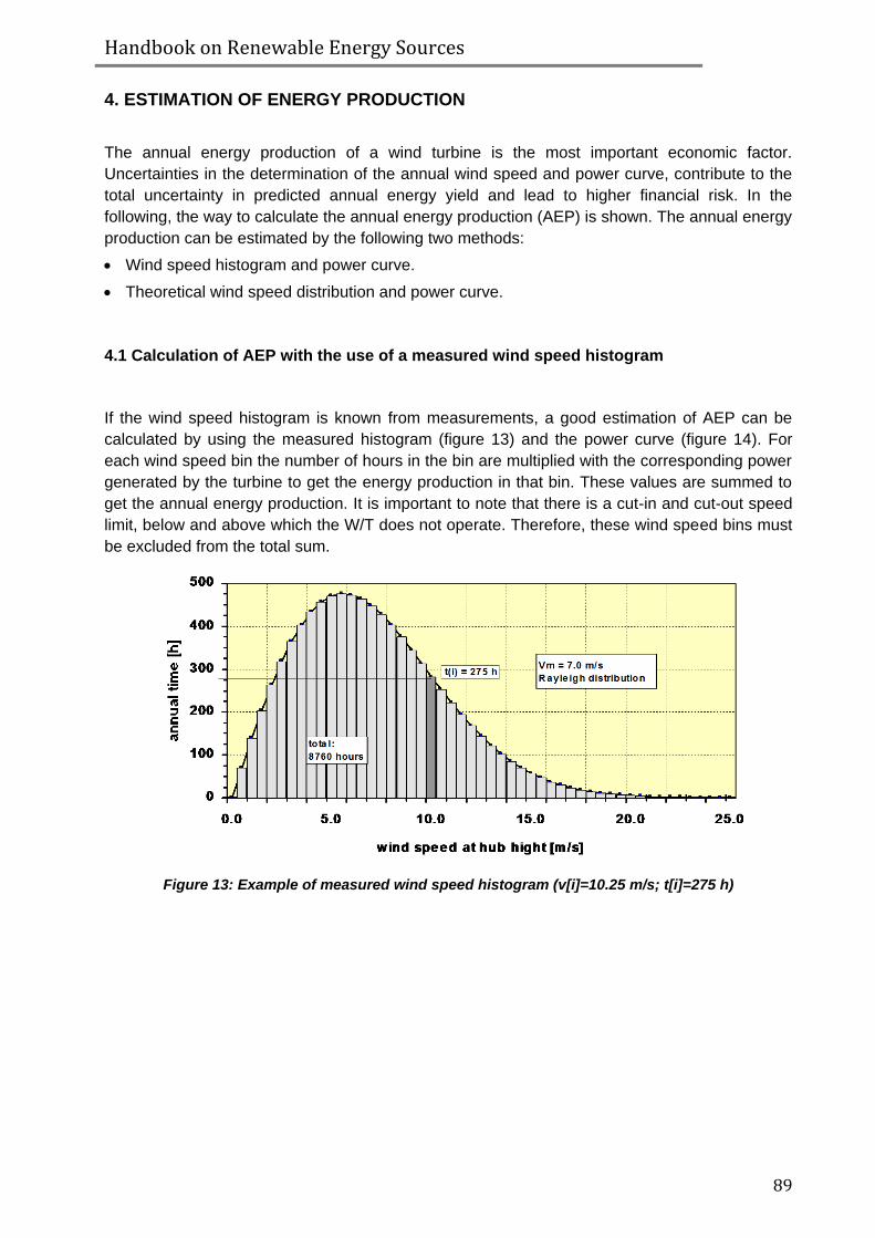
Handbook on Renewable Energy Sources
89
4. ESTIMATION OF ENERGY PRODUCTION
The annual energy production of a wind turbine is the most important economic factor.
Uncertainties in the determination of the annual wind speed and power curve, contribute to the
total uncertainty in predicted annual energy yield and lead to higher financial risk. In the
following, the way to calculate the annual energy production (AEP) is shown. The annual energy
production can be estimated by the following two methods:
Wind speed histogram and power curve.
Theoretical wind speed distribution and power curve.
4.1 Calculation of AEP with the use of a measured wind speed histogram
If the wind speed histogram is known from measurements, a good estimation of AEP can be
calculated by using the measured histogram (figure 13) and the power curve (figure 14). For
each wind speed bin the number of hours in the bin are multiplied with the corresponding power
generated by the turbine to get the energy production in that bin. These values are summed to
get the annual energy production. It is important to note that there is a cut-in and cut-out speed
limit, below and above which the W/T does not operate. Therefore, these wind speed bins must
be excluded from the total sum.
Figure 13: Example of measured wind speed histogram (v[i]=10.25 m/s; t[i]=275 h)

Handbook on Renewable Energy Sources
90
Figure 14: Example of measured power curve at standard air density (1.225 kg/m³)
(p[i]=345 kW; v[i]=10.25 m/s)
Figure 15: Example of estimated energy in bin i (E[i]=95 MWh)
The total energy production in one year (AEP) (see fig. 15) is: E P i h ii
i n
[ ]* [ ]1
4.2 Calculation of AEP using a theoretical wind speed distribution
If the wind speed distribution at the site is unknown, a histogram can be calculated from the
known or estimated average wind speed. As mentioned previously, two theoretical distributions
are mainly in use to calculate the wind speed: the Weibull distribution, which uses two
parameters, one shape parameter and a scale parameter, and a mono-parametric one, the
Rayleigh distribution, which is identical to a Weibull distribution with a shape factor of two
(normally preferred, as the shape parameter is often unknown).

Handbook on Renewable Energy Sources
91
The Rayleigh distribution is written as:
F v e
v
v( )
1 4
2
where F(v) is the Rayleigh cumulative distribution for wind speed and v is the annual average
wind speed at hub height. Then, the annual energy production is:
AEP F v F vP P
i i
i i
i
N
876021
1
1
* ( ) ( )
where N is the number of bins, vi is the wind speed v in bin i, and Pi is the averaged power
output in bin i.
5. SITE FACTORS THAT AFFECT THE SELECTION
Many other factors besides the wind regime have to be considered in the final choice of the
optimum site for installing a wind power plant. These briefly include:
access to the grid;
local road access;
local environmental effects, including the landscape classification;
closeness of local habitation;
the effect of noise;
interference in TV and radio signals, etc.
Wind farm locations and the associated weather conditions have posed engineers with
enormous challenges in meeting wind farm design requirements and installing systems. Poor
site access can hinder the delivery of large and heavy components, bare rock can make
earthing almost impossible, and rain and mist can result in water ingress in the cable
terminations and joints. Issues such as transformer location and generator voltage have also
become more important as wind turbine size has increased. A particular issue for electrical
systems of wind farms is the choice of the site distribution system voltage.
5.1 Site access
Construction and operation of a wind generation facility requires use of heavy equipment for site
preparation, transport of construction supplies and project components, and for the erection of
turbines and electric poles and towers. Thus, there may be a potential for wind projects to affect
rural roads designed for infrequent traffic or lightweight vehicles. Existing roadbeds may have to
be rebuilt or reinforced to support such additional loads without degradation, and the frequency
of scheduled maintenance on these roads may have to be increased.
Constructing new roads on slopes to gain access to the ridge tops also opens the potential for
erosion that can produce long-term visual changes in the site area. Thus, reducing the need for
roads within a wind development reduces project infrastructure costs, erosion and water quality
problems, as well as visual impacts. Using airlift for transport of turbine components and turbine
installation, major maintenance works, etc. greatly reduce the size and placement of roads in

Handbook on Renewable Energy Sources
92
remote locations or sensitive visual areas. This also would lower impacts on public and rural
roads and provide for quicker installation, but it is expensive and may be infeasible for larger
turbines.
In general, it is advisable to:
use of roadless construction and maintenance techniques in order to reduce temporary and
permanent land loss;
restrict most vehicle travel to existing access roads;
limit the number of new access roads, width of new roads, and avoid or minimize cut and fill;
construct new access roads that follow existing contours to the greatest extent possible.
5.2 Grid integration
5.2.1 Public electricity transmission & distribution system
Wind turbines are usually located in rural or upland areas, where the electrical connection to the
nearest electricity substation can be weak, and the local demand for electricity may be much
less than the wind generation capacity. One way of defining the "strength" of the electricity
network is by the fault level, which is a measure of the current that will flow when there is a fault
on a network. At the end of a long electricity circuit the fault level is much lower than at the
centre of an interconnected network, for example in a town or industrial development.
At a low fault level site, the impact of wind turbines can be great enough to disturb other local
consumers. For this reason, it is sometimes necessary to reinforce the network, or connect the
wind turbines to a higher voltage or stronger part of the network further away. This will increase
costs. Higher-voltage systems, such as the 400 kV or 275 kV transmission systems, have high
fault levels. In general, the lower the voltage the weaker the system will be. The distribution
system voltages in rural areas of most EU countries are 132, 33 and 11 kV. The 11 kV system
is the most extensive one, but it is unlikely to support more than one to three megawatts (MW)
of generation.
The term Public Electricity Supplier (PES) is used herein for the company that operates the
local electricity network (in most cases this is synonymous with the term REC, or Regional
Electricity Company). The PES is responsible for the safe and economic operation of its system
and has obligations to maintain satisfactory quality of supply to the users of its system, while it
is not necessarily the purchaser of the electricity generated by the wind turbines. The PES
should be advised of the proposed scheme at an early stage.
PES engineers will carry out initial studies to ascertain the technical feasibility of the project and
can then quote a cost for connection, which may determine whether or not the project will
proceed (the PES may charge for this service). Costs will depend on the size of the
development, the distance from the nearest connection point, and the connection voltage. This
last point may be the most important, as connection costs can render small projects far from the
existing system completely uneconomic. This is best discovered before much effort has been
expanded.

Handbook on Renewable Energy Sources
93
In rural or upland areas, it is most likely that the nearest point on the local electricity network is
an overhead line, rather than underground cable. A number on a pole or tower (pylon) may be
found, which will help the PES engineers locate the proposed site on their system maps, and
they will then be able to define the voltage of the line. Ordnance Survey grid references can
also be used. Any overhead line with only two wires is carrying a single-phase system and will
normally require reinforcement if generators are to be installed.
5.2.2 Design of the connection
Determining the right technical/economic design of the electric power collection system for a
wind farm and its connection to the electricity network is a multi-parameter optimization process
requiring extensive experience on the part of the designer/engineer, as well as the availability of
modern power system computational tools to facilitate the task of finding and documenting the
right solution.
A number of issues need to be considered in this stage, including:
Connection voltage; this has a significant effect on the cost of the connection. For example,
a new 33 kV line will cost considerably more than connecting into an existing 11 kV circuit;
however, a new 11 kV line can cost more than a new 33 kV line, for the same wind farm
output.
Distribution voltage within the wind farm.
Arrangement of transformers and wind turbines.
Earthing; the electrical installation must be adequately earthed to ensure that people or
equipment are not harmed by electrical faults or lightning strikes, and to comply with the
Electricity Supply Regulations and Safety at Work Regulations. This is a complex issue and
should not be underestimated.
Protection; equipment must be provided to ensure that the wind turbine or wind farm is
automatically disconnected when there is a fault on the network. Similarly, the network must
be protected from the effects of a fault within the wind farm.
Metering; the electricity is metered at the point of connection to the local network. Meters
are required for both exported and imported power (which can occur in very low winds), and
for reactive power. Metering accuracy and cost increases with the size of the wind farm.
Usually, the overall layout of the wind farm is based on an optimisation of the production of the
farm with regard to the sites of the individual turbines and the accessibility of the turbines - i.e.
infrastructure. The short circuit contribution from the grid is an important parameter and,
depending on the availability and ratings of the electrical equipment - transformers, cables, ring
main units, circuit breakers, etc. –, a layout satisfying the basic electrical design requirements is
chosen and verified through fault current calculations.
Finally, the total lifetime losses - and their present net value - are evaluated to see if the use of
equipment with lower losses can be justified from an economic point of view. The loss
calculations are based on the production profile of the wind farm, calculated from the
parameters describing the wind - the Weibul parameters -, and the power curve of the wind
turbines in question.
Handbook on Renewable Energy Sources
94
5.3 Other issues affecting the selection of the site
Wind power plants offer several important environmental advantages over conventional power
plants running on coal, oil, or natural gas; namely, they use no fuel, emit no air pollutants,
greenhouse gases, or toxic wastes, and consume no water or other scarce resources.
Nevertheless, wind plants can rise environmental and community concerns. For example, they
generate noise and can be visually intrusive for residents living near them. They also can
disturb wildlife habitats and cause injury or death to birds.
Fortunately, despite past mistakes, these and other potential problems need not pose a serious
obstacle to wind development in most cases. Through conscientious planning research, proper
design, and early and frequent consultations with affected communities, wind plant developers
can identify and address the most serious issues before substantial investments are made in
new wind projects. Utilities, government agencies, environmental organizations, and others
need to work with developers to ensure that such effective strategies are implemented.
It is in both the developer's and the public's interest that the siting process address all legitimate
issues in an open, fair and unbiased fashion, while minimizing costs for the participants and
delays in reaching a decision. In some cases, the result of the process may be to rule out a
proposed site for wind development. In other cases, it may be determined either that the issues
raised are not of serious concern, or that specific measures can be taken to address them.
5.3.1 Issues concerning local communities
Building and operating a wind plant involves many of the same activities as building and
operating a conventional power plant, including road construction, land clearing, truck traffic,
and the construction of transmission lines. Not surprisingly, activities such as these sometimes
arouse significant community concerns. In addition, wind projects raise unique community
issues, mostly concerning their visual impacts and noise.
Land use considerations
Unlike most power plants, wind generation projects are land intrusive rather than land intensive.
On a megawatt (MW) output basis, the land required for a wind project exceeds the amount of
land required for most other energy technologies. However, while wind facilities may extend
over a large geographic area and have a broad area of influence, the project physical “footprint”
covers a relatively small portion of that land. A 50 MW wind facility, for example, may occupy a
1,500-acre site, but the amount of land actually occupied by the wind energy facilities may only
be three to five percent of the total acreage, leaving the rest available for other compatible uses.
Because wind generation is limited to areas where weather patterns provide a relatively long
season of strong and consistent wind resources, the development of wind projects worldwide
has occurred primarily in rural and relatively open areas. These lands are often used for
agriculture, grazing, recreation, open space, scenic areas, wildlife habitat, forest management,
and seasonal flood storage. Wind development typically is compatible with the agricultural or
grazing use of a site.
Although these uses may be interrupted during construction, only intensive agricultural uses
may be reduced or modified during project operation. Development of wind projects may affect

Handbook on Renewable Energy Sources
95
other uses on or adjacent to a site, or in the surrounding region. Some parks and recreational
uses that emphasize wilderness values and reserves dedicated to the protection of wildlife -
particularly birds - may not be compatible with nearby wind developments.
Other uses, such as open space preservation, growth management or non-wilderness
recreation facilities, may be compatible depending on setbacks, the nature of on-site
development, and the effect on resources of regional importance. The variables that may
determine land use impacts include: the site’s topography; the size, number, output and spacing
of the turbines; the location and design of roads; whether accessory facilities are consolidated
or dispersed; and whether the electric lines are overhead or underground.
Visual impacts
Wind turbines are highly visible structures. Modern wind turbine towers stand 30 to 50 meters
above the ground, not counting the blades of the rotor that may be up to 40 meters in diameter.
In addition, the turbines often are deployed in arrays of a dozen or more machines on
conspicuous ridges or hilltops. Whether the visual impact of wind turbines generates complaints
depends partly on the setting in which they are located.
In many agricultural areas in USA, developers have encountered relatively few problems in
winning community acceptance of wind projects. This makes sense, considering that windmills
were a common sight on American farms until the mid-20th century. It helps, too, that agricultural
landowners often directly benefit from wind projects through land rents and fees paid by plant
owners. In other settings community acceptance may be a more serious problem.
Sometimes, wind plants proposed near residential areas have aroused strong opposition from
homeowners and real estate developers. In one case, residents opposing the Cordelia Hills
wind project, northeast of San Francisco, reportedly did not want to see turbines sited nearby,
even though the hills chosen for the project already had numerous electronic relays and
transmission lines. Needless to say, siting a wind project near a national park or wilderness
preserve may incite complaints from local environmental organizations and activists.
Whatever the setting, steps can be taken to reduce the number of complaints by making wind
turbines less obtrusive and more pleasing to the eye. For example, tubular towers are less
offensive than lattice towers, and partly for this reason they now are preferred by most wind
developers. Combined with the sleek, minimalist appearance of some modern wind turbine
housings and rotors, the overall effect can be quite attractive.
Careful attention must be given to how a wind turbine array is set against the landscape. A well-
ordered array gives the appearance of purpose and efficiency, whereas one that appears to be
scattered haphazardly leaves the impression of aimlessness and confusion. Following the
contours of a ridge will make a line of wind turbines blend more easily with the surroundings.
Taking steps to avoid scarring the land with unsightly roads and clearings is important, as is
eliminating unnecessary clutter by burying transmission lines and hiding buildings and other
structures behind ridges or vegetation.
A valuable process tool for the assessment of potential project impacts to sensitive visual
resources is the preparation and use of visual simulations. Evaluation of these simulations
allows the project developer, permitting agencies, and the public to see the site as it is, and to

Handbook on Renewable Energy Sources
96
see the changes the project will bring to the existing setting and any sensitive resources. After
viewing the simulations of important vantage points, all stakeholders can be involved in
adjusting project layout and design to minimize potential impacts.
Efforts to educate and inform nearby communities about wind energy and its benefits also can
help lessen opposition on aesthetic grounds. For example, there is a tendency for people who
pass by a wind power plant to notice the few machines that are not operating rather than the
majority that are. This can lead people to think wind technology does not work. Letting people
know that it is normal for some turbines to be stopped at any time (because of wind variations
and maintenance needs) may help alleviate this public relations problem.
Noise
By and large, those affected by the noise generated by wind turbines live within a few
kilometres of a large wind power plant or within several hundred metres of a small plant or
individual turbine. Although the noise at these distances is not great - a 300kW turbine typically
produces less noise at 120 metres than does light traffic 30 metres away - it nevertheless is
sufficient to be heard indoors and may be especially disturbing in the middle of the night, when
traffic and household sounds are diminished (see Table 3).
Table 3: Typical sound pressure levels
When planning a wind turbine project, careful consideration should be given to any noise that
might be heard outside nearby houses. Inside, the level is likely to be much lower, even with
windows open. Predicting the noise that will be produced when the wind is blowing from the
turbines towards the houses usually assesses the potential noise impact. This is then compared
to the background noise that already exists in the area, without the wind farm operating.
Zoning ordinances developed by some communities for wind developments address this
problem by specifying setbacks and allowable noise levels to minimize disturbance to
neighbours. Palm Springs, for example, requires that no wind turbine be located closer than 370
Handbook on Renewable Energy Sources
97
metres from any residence, hotel, hospital, school, library or convalescent home, except where
topography permits an exception to be made. At specified distances, noise is required to be less
than 55 decibels, approximately the volume generated by wind blowing through trees 15 metres
away.
Significant progress has been made in reducing turbine noise since the first machines were
installed in the early 1980s. The larger machines now on the market generate less noise (per
unit of energy output) than the smaller machines they replaced, in part because of slower rotor
tip speeds and careful design and manufacture of blade airfoils and trailing edges. Overall, with
proper attention to setback distances and sound-reduction engineering, few, if any, residents
will be affected by wind turbines noise.
Electromagnetic interference (EMI)
Electromagnetic interference is the disruption of electromagnetic signals used in communication
technologies including radio, television and microwaves. It has been discussed as a possible
problem with certain aspects of wind generation, primarily the rotating blades of wind turbines
and very high voltage electric transmission lines. Turbine blades most easily reflect UHF
television signals, while television reception within five kilometres (UHF) or 6/5 kilometre (VHF)
of a turbine of sufficient size may be affected. The degree of interference depends on the blade
material, turbine location relative to the signal path, and turbine size.
Interference with FM radio reception has not been reported. Microwave repeating stations are
often located on remote and rural hilltops. These stations rely on unobstructed line-of-sight
paths for their signals and consequently may be affected by wind projects, which intrude into the
beam corridor. In addition, the electrical circuits in the turbine may transmit an electromagnetic
signal (noise) if it is not properly installed and maintained. Thus, contacts with the operators of
microwave communication stations are necessary in order for wind projects to avoid creating
interference.
5.3.2 Avoiding wildlife and other sensitive areas
Birds
The potential effects of wind energy development on wildlife and wilderness areas have
attracted attention in recent years. The issue first rose to prominence in the late 1980s, when it
was found that birds, especially federally protected golden eagles and red-tailed hawks, were
being killed by wind turbines and high-voltage transmission lines at California's Altamont Pass.
The discovery sparked opposition to the Altamont Pass project among some environmental
activists and aroused the concern of the U.S. Fish and Wildlife Service, which is responsible for
enforcing federal species-protection laws.
Since then, problems have been noted in other locations too. Birds have been reported killed at
wind power plants in Tarifa, Spain (one of two major points of bird migration across the
Mediterranean Sea), and at various wind plants in northern Europe. These incidents have
resulted in a heightened awareness of wind power's potential environmental impacts among
both U.S. and European conservation groups. The long-term implications of the bird issue for
the wind industry are as yet unclear, however.
Handbook on Renewable Energy Sources
98
It seems likely that serious conflicts will be confined mainly to areas where large numbers of
birds congregate or migrate (as in Tarifa), or where protected species are affected (as in
Altamont Pass). However, this could encompass quite a few locations, because some of the
traits that characterize a good wind site also happen to be attractive to birds. For example,
mountain passes are frequently windy because they provide a channel for winds passing over a
mountain range; for precisely the same reason, they are often the preferred routes for migratory
birds.
Just because birds frequent a particular area does not necessarily mean a wind power plant
should not be built there. Several factors need to be considered in making this decision. One is
whether the birds are likely to come into conflict with the wind turbines. Research on bird
numbers and behaviour can give an indication of the likelihood that birds will encounter wind
turbine blades.
Another consideration is the likely significance of bird deaths and injuries for local bird
populations. The ideal is for no birds to be killed, but this will not be practical in many cases. A
more scientifically meaningful standard for measuring the severity of impact might be whether
the deaths will result in a significant decrease in the total population or a significant increase in
the total mortality of the affected species.
If preliminary research indicates that a wind project is unlikely to seriously affect bird
populations, further studies may be needed to verify this conclusion. These could include
monitoring baseline bird populations and behaviour before the wind project begins, then
simultaneously observing both a control area and the wind site during construction and initial
operation. In certain cases, operational monitoring might have to continue for years.
In recognition of the potential seriousness of the bird issue, the wind energy industry is
collaborating with various national/regional agencies and environmental organizations to
develop a suitable avian research program and siting guidelines. While disagreements are
inevitable, all parties recognize their common interest in seeing wind energy succeed both in
European Union and the United States, without causing serious harm to birds and other wildlife.
Wilderness habitat
Some studies have shown that birds and other animals tend to avoid nesting or hunting for food
in the immediate vicinity of wind turbines. In addition, activities such as road construction and
tree clearing can destroy or disrupt habitats and allow the introduction of unwanted species. The
problem is compounded by the fact that some of the best prospective wind sites are located in
remote, mountainous areas that are home to many different species of plants and animals.
Because of these concerns, some ecologically sensitive areas (even if not explicitly protected
by national or regional laws) should be off-limits to wind power projects. However, in other
cases options may exist for mitigating or offsetting any habitat impacts that occur. For example,
developers can invest in off-site remediation, such as tree planting or the creation of habitats for
species displaced by wind projects. The exact measures needed, if any, will depend on the
particular location and species concerned and should be determined in consultation with the
appropriate national and regional agencies and environmental organizations.

Handbook on Renewable Energy Sources
99
Cultural and paleontological considerations
For certain types of cultural resources, the physical setting and vicinity of the resource site
contribute materially to its value. In this case, the area of potential impact may include areas
within audible or visual distance of the sensitive resource. For example, wind generation sites
are often located on the sides and ridges of hills and may be near the coast or shoreline of large
water bodies. Native peoples also used such areas for traditional resource harvest and
seasonal and religious ceremonies. Thus, during project and site design, cultural and fossil
resources sites should be avoided and protected.
Wind development in such locations has a greater potential to affect large-scale, aboveground
cultural resources or resource settings. The area of potential impact may extend only a few tens
of metre or may extend out to one-quarter kilometre or more. This type of impact is most likely
to be associated with long-standing resource collection areas, landmarks, or sacred areas and
features. Cultural resource impacts in these areas may also include concerns about disturbance
of traditional practices due to noise and visual impacts.
The extent of the potential for impacts will vary with the topography, vegetation, the extent of the
resource area, and the presence or absence of other developments. Techniques for data
recovery and mapping of the fossil record may make it unnecessary to redesign or modify the
turbine layout design. On the other hand, the location of most wind turbine towers and related
access roads, transmission lines, and service or maintenance structures can usually be
adjusted during the design phase to avoid impacts to known surface or sub-surface cultural and
fossil resources.
5.4 Planning for wind development
In general, it is helpful for the site selection procedure if communities, such as towns and
counties, have implemented zoning amendments for wind plants, and for each type of zone
(commercial, industrial or agricultural) to exist standards in the following areas:
Wind turbine size, including maximum rotor size, minimum and maximum height, tower
height, etc.
Installation and design, including the tower and rotor, as well as electrical safety, utility
notification, warning signs and tower access.
Siting, including setbacks from plant boundaries and neighbouring facilities, aesthetic design
(such as tubular or lattice towers) and clearances from electrical lines.
Nuisance concerns, such as noise regulations and television or radio interference.
Other regulations, including insurance, public access to wind facilities, and repair,
maintenance and decommissioning requirements.
Some local agencies, recognizing the potential for wind generation, have formally identified
wind resource areas (WRAs) in their plans in order to facilitate permitting and development of
wind generation in preferred locations, and have prepared maps of these areas showing
information such as wind speed and duration, topographic features, site characteristics, existing
roads and facilities, potentially sensitive land uses, etc. Thus, they can provide up-front
guidance to developers on where and how to locate wind projects, in order to be consistent with
existing land uses and the environment.

Handbook on Renewable Energy Sources
100
6. CRES Wind Atlas Methodology and application results
6.1 Introduction
When a number of measurements covering an area are available then it might be of interest to
exploit these discrete data for an assessment of the wind potential, treating the area as a
continuum instead of a grid of points. The methodology described in the following results in the
assessment of the wind potential of a large area, without any limitations regarding its size. It
was successfully used to predict the wind potential of Greece, yielding satisfactory results on a
pretty fine mesh with surface resolution of 150m for the entire country.
The computational method developed by CRES achieves to establish an interpolation
procedure that receives as input a substantial number of measurements and produces a
prediction at an arbitrary point inside the area of interest. The procedure undertaken for the
measurements is beyond the scope of the interpolation method, as long as there are sufficient
points where wind data are available to describe the mesoscale effect.
6.2 Description of the methodology
The methodology is derived from the assumption that the wind flow at high altimeters is inviscid,
free from the influence of the surface boundary layer, governed strictly by meteorological
mechanisms. On the other hand, the boundary layer phenomena are predominant close to the
surface. There, the combined action of the topography and the boundary layer is enough to
determine the wind speed and direction at any given point. In essence, a three-dimensional
boundary correction method is introduced.
The whole calculation procedure is a two-step one. First, the three-dimensional space, which is
defined by the surface and reaches up to a few kilometres in altitude, is analysed employing a
potential flow code (mass conservation). The code works using normalized variables, imposing
a unity velocity boundary condition at the upper side of the mesh. Because of the need to cover
very large geographical areas, a multi-block approach is followed.
The area is divided into a large number of blocks, each of which is independently handled (see
figure 16 ). Another set of blocks is generated from the first, defining a mesh of staggered with
respect to the original series blocks (figure 17). These two sets of blocks are used together to
generate the final results, through extension, averaging and interpolation. Taking advantage
from the fact that potential flow results far from the boundaries are insensitive to perturbations of
boundary conditions, the above procedure yields a smooth and continuous solution at the block
interfaces. Individual calculations are performed for each one of the chosen wind directions.

Handbook on Renewable Energy Sources
101
EXTENSION
STAGGERED GRID
INITIAL GRID
Figure 16: The Multi-Block modeling approach for the case of Greece (left) and the staggering of
the calculation grid (right)
In a second step, a boundary layer correction is applied in order to introduce the viscous
phenomena to the calculation. A simplified approach is followed for the viscous correction,
derived from flat terrain boundary layer theory and the assumption of constant roughness (as
long as roughness maps are not available). Correction is performed on a point-by-point basis.
This simple method presents the significant advantage that the mass rate is maintained.
However, it is possible to substitute this by any boundary layer correction procedure.
At the end of this two-step procedure the flow field is completely defined, although still
normalized by the wind speed at the upper bound. The normalization assumption that the wind
speed at high altimeter is equal to unity is not equivalent to suggesting that it is constant too. On
the contrary, it is known to exhibit significant variation. At this stage of the methodology, the
intention is to calculate the wind speed at the upper bound. To this end, the available
measurements are used.
For each point in the geographical area were measurements exist, it is possible to calculate the
average wind speed for each direction of interest. Using this value, and the respective value at
the computational grid node, the wind speed at the upper bound of the specific point can be
predicted. This way, the measurements are used to predict the wind speed at a grid point at the
upper bound. Interpolation of these values yields the wind speed at every point of the upper
bound. The normalized values in the complete geographical area and at every height can then
be converted to actual wind speeds.
The results attained up to this point still cover independently each direction. Using time-
averaging information (probability density function of the wind direction), also yielded through
the measurements, the average wind speed may be calculated at each point. Using this
procedure the Weibull distribution shape factors can also be derived, which might be of interest
for a better prediction of the electrical energy production by wind turbines in an area. Figure 6.2
presents the wind map of Peloponnese, i.e. the theoretical wind potential of Peloponnese, as

Handbook on Renewable Energy Sources
102
calculated based on the measurements and simulations, the contour lines and the local
authorities.
Figure 17: Theoretical wind potential of Peloponnesus

Handbook on Renewable Energy Sources
103
GEOTHERMAL ENERGY
1. GEOTHERMAL ENERGY AND THE ENVIRONMENT
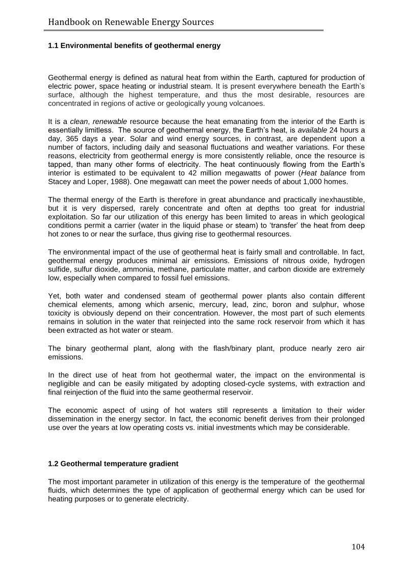
Handbook on Renewable Energy Sources
104
1.1 Environmental benefits of geothermal energy
Geothermal energy is defined as natural heat from within the Earth, captured for production of electric power, space heating or industrial steam. It is present everywhere beneath the Earth’s surface, although the highest temperature, and thus the most desirable, resources are concentrated in regions of active or geologically young volcanoes.
It is a clean, renewable resource because the heat emanating from the interior of the Earth is essentially limitless. The source of geothermal energy, the Earth’s heat, is available 24 hours a day, 365 days a year. Solar and wind energy sources, in contrast, are dependent upon a number of factors, including daily and seasonal fluctuations and weather variations. For these reasons, electricity from geothermal energy is more consistently reliable, once the resource is tapped, than many other forms of electricity. The heat continuously flowing from the Earth’s interior is estimated to be equivalent to 42 million megawatts of power (Heat balance from Stacey and Loper, 1988). One megawatt can meet the power needs of about 1,000 homes.
The thermal energy of the Earth is therefore in great abundance and practically inexhaustible, but it is very dispersed, rarely concentrate and often at depths too great for industrial exploitation. So far our utilization of this energy has been limited to areas in which geological conditions permit a carrier (water in the liquid phase or steam) to ‘transfer’ the heat from deep hot zones to or near the surface, thus giving rise to geothermal resources.
The environmental impact of the use of geothermal heat is fairly small and controllable. In fact, geothermal energy produces minimal air emissions. Emissions of nitrous oxide, hydrogen sulfide, sulfur dioxide, ammonia, methane, particulate matter, and carbon dioxide are extremely low, especially when compared to fossil fuel emissions.
Yet, both water and condensed steam of geothermal power plants also contain different chemical elements, among which arsenic, mercury, lead, zinc, boron and sulphur, whose toxicity is obviously depend on their concentration. However, the most part of such elements remains in solution in the water that reinjected into the same rock reservoir from which it has been extracted as hot water or steam.
The binary geothermal plant, along with the flash/binary plant, produce nearly zero air emissions.
In the direct use of heat from hot geothermal water, the impact on the environmental is negligible and can be easily mitigated by adopting closed-cycle systems, with extraction and final reinjection of the fluid into the same geothermal reservoir.
The economic aspect of using of hot waters still represents a limitation to their wider dissemination in the energy sector. In fact, the economic benefit derives from their prolonged use over the years at low operating costs vs. initial investments which may be considerable.
1.2 Geothermal temperature gradient
The most important parameter in utilization of this energy is the temperature of the geothermal fluids, which determines the type of application of geothermal energy which can be used for heating purposes or to generate electricity.

Handbook on Renewable Energy Sources
105
Going from the surface of the earth towards the core, we observe that the temperature progressively increases with depth by 3 °C, on average, every 100 meters (30 °C/km). This is called geothermal gradient. For example, if the temperature within the first few metres below ground-level, which on average corresponds to the mean annual temperature of the external air, is 15 °C, then we can reasonably assume that the temperature will be about 65°-75 °C at 2000 m depth, 90°- 105 °C at 3000 m and so on for a further few thousand metres (figure 1).
The regions of interest for applications of geothermal energy are those where the geothermal gradient is in excess of normal. In some areas, either due to volcanic activity during a recent geological age, or due to the rise of hot water from very deep levels through fissures, the geothermal gradient is significantly greater than the average, so to have temperatures of 250-350°C at a depth of about 2000-4000 m.
Such “hot” zones generally are near the boundaries of the dozen or so slabs of rigid rock (called plates) that form the Earth’s lithosphere, which is composed of the Earth’s crust and the uppermost, solid part of the underlying denser, hotter layer (the mantle).
Figure 1 – Temperature versus depth for various geothermal gradient; ground temperature assumed to be 17° C.
The mean terrestrial heat flow of continents and oceans is 65 and 101 mWm-2, respectively, which, when areally weighted, yield a global mean of 87 mWm-2 (Pollack et al., 1993

Handbook on Renewable Energy Sources
106
2. BACKGROUND ON GEOTHERMAL ENERGY
2.1 Geothermal Systems
A geothermal system is made up of some main elements: a heat source, a reservoir, a fluid, which is the carrier that transfers the heat, a recharge area and an impermeable cap rock to seal the aquifer. The heat source can be either a very high temperature (> 600 °C) magmatic intrusion that has reached relatively shallow depths (5-10 km) or, as in certain low-temperature systems, the Earth's normal temperature, which, as we explained earlier, increases with depth. The reservoir is a volume of hot permeable rocks from which the circulating fluids (water or steam) extract heat. The reservoir is generally overlain by either primarily impervious layers or by rocks whose poor permeability is due to self-sealing phenomena that is the deposition of minerals in the rock discontinuities and pores. The reservoir is connected to a superficial recharge area through which the meteoric waters can replace or partly replace the fluids that escape from it through springs or are extracted by boreholes. The geothermal fluid is water, in the majority of cases meteoric water, in the liquid or vapour phase, depending on its temperature and pressure. This water often carries with it chemicals and gases such as CO2, H2S, etc. Figure 2 is a greatly simplified representation of an ideal geothermal system.
The mechanism underlying geothermal systems is by and large governed by fluid convection. Convection occurs because of the heating and consequent thermal expansion of fluids in a gravity field; heat, which is supplied at the base of the circulation system, is the energy that drives the system. Heated fluid of lower density tends to rise and to be replaced by colder fluid of high density, coming from the margins of the system. Convection, by its nature, tends to increase temperatures in the upper part of a system as temperatures in the lower part decrease (White, 1973).
The phenomenon we have just described may seem quite a simple one but Geothermal systems also occur in nature in a variety of combinations of geological, physical and chemical characteristics, thus giving rise to several different types of system.
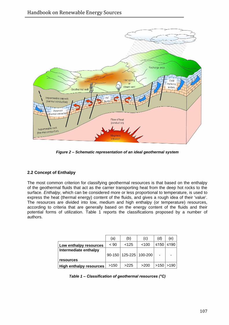
Handbook on Renewable Energy Sources
107
Figure 2 – Schematic representation of an ideal geothermal system
2.2 Concept of Enthalpy
The most common criterion for classifying geothermal resources is that based on the enthalpy of the geothermal fluids that act as the carrier transporting heat from the deep hot rocks to the surface. Enthalpy, which can be considered more or less proportional to temperature, is used to express the heat (thermal energy) content of the fluids, and gives a rough idea of their 'value'. The resources are divided into low, medium and high enthalpy (or temperature) resources, according to criteria that are generally based on the energy content of the fluids and their potential forms of utilization. Table 1 reports the classifications proposed by a number of authors.
(a) (b) (c) (d) (e)
Low enthalpy resources < 90 <125 <100 ≤150 ≤190
Intermediate enthalpy
resources
90-150 125-225 100-200 - -
High enthalpy resources >150 >225 >200 >150 >190
Table 1 – Classification of geothermal resources (°C)

Handbook on Renewable Energy Sources
108
Source:
(a) Muffler and Cataldi (1978).
(b) Hochstein (1990).
(c) Benderitter and Cormy (1990).
(d) Nicholson (1993).
(e) Axelsson and Gunnlaugsson (2000)
High temperature fields used for conventional power production are largely confined to areas with young volcanism, seismic and magmatic activities. Low temperature resources can, on the other hand, be found in most countries. They are formed by the deep circulation of meteoric water along the faults and fractures, and by water residing in high-porosity rocks, such as sandstone and limestone, at sufficient depths for the water to be heated by the earth’s geothermal gradient.
Frequently a distinction is made between water- or liquid-dominated geothermal systems and vapour-dominated (or dry steam) geothermal systems (White, 1973). In water-dominated systems liquid water is the continuous, pressure-controlling fluid phase. Some vapour may be present, generally as discrete bubbles. These geothermal systems, whose temperatures may range from < 125 to > 225 °C, are the most widely distributed in the world. Depending on temperature and pressure conditions, they can produce hot water, water and steam mixtures, wet steam and, in some cases, dry steam. In vapour-dominated systems liquid water and vapour normally co-exist in the reservoir, with vapour as the continuous, pressure-controlling phase. Geothermal systems of this type, the best-known of which are Larderello in Italy and The Geysers in California, are somewhat rare, and are high-temperature systems. They normally produce dry-to-superheated steam.
Another division between geothermal systems is that based on the reservoir equilibrium state (Nicholson, 1993), considering the circulation of the reservoir fluid and the mechanism of heat transfer. In the dynamic systems the reservoir is continually recharged by water that is heated and then discharged from the reservoir either to the surface or into underground permeable formations. Heat is transferred through the system by convection and circulation of the fluid. This category includes high temperature (>150 °C) and low-temperature (<150 °C) systems. In the static systems (also known as stagnant or storage systems) there is only minor or no recharge to the reservoir and heat is transferred only by conduction. This category includes low temperature and geopressured systems.
3. UTILIZATION OF GEOTHERMAL RESOURCES
Electricity generation is the most important form of utilization of high-temperature geothermal resources (> 150 °C). The medium-to-low temperature resources (< 150 °C) are suited to many different types of application. The classical Lindal diagram (Lindal, 1973) shows the possible uses of geothermal fluids at different temperatures (Figure 3, with the addition of electricity generation from binary cycles). Fluids at temperatures below 20 °C are rarely used and in very particular conditions, or in heat pump applications.

Handbook on Renewable Energy Sources
109
Figure 3 – Diagram showing the utilization of geothermal fluids (derived from Lindal, 1973)
3.1 Direct heat uses
In the case of temperature lower than 90 °C, the geothermal water can be used directly rather than converting it to electricity. The best known form of utilizations include space heating with water air-heaters or floor heating system, agricultural applications, aquaculture and some industrial uses. When water temperatures are below 40°C, heat pumps for space heating and cooling are applied. If underground water is not available, heat pumps may be combined with earth heat exchangers.
3.1.1 Principles of heat pumps
A heat pump (figure 4) is a thermal machine that allows for the extraction of heat from the ground or from aquifers at shallow depth (tens or hundreds of meters) and low temperature and transfers it at higher temperature into the environment to be heated. The advantage of heat pumps lies in the fact that, for every unit of electrical energy consumed, about three units of energy under the form of heat are obtained with the contribution of geothermal water.
When cooling, heat is extracted from the space and dissipated into the Earth; when heating, heat is extracted from the Earth and pumped into the space.
A heat pump is subject to the same limitations from the second law of thermodynamics (any energy transformation involves a dissipation of a share of it in the form of heat at low temperature, no longer usable) as any other heat engine and therefore a maximum efficiency

Handbook on Renewable Energy Sources
110
can be calculated from the Carnot cycle. Heat Pumps are usually characterized by a coefficient of performance which is the number of units of energy delivered to the hot reservoir per unit work input.
Figure 4 – Geothermal Heat Pumps
3.2 Electricity generation
High enthalpy geothermal energy is used mostly for electricity production.
The typical geothermal system used for electric power generation must yield approximately 10 kg of steam to produce one unit (kWh) of electricity. Production of large quantities of electricity, at rates of hundreds of megawatts, requires the production of great volumes of fluid. Thus, one aspect of a geothermal system is that it must contain great volumes of fluid at high temperatures or a reservoir that can be recharged with fluids that are heated by contact with the rock.
The three basic types of geothermal electrical generation facilities are binary, dry steam (referred to as “steam”), and flash steam (referred to as “flash”) when the pressure on hot water (usually above 100°C) is reduced. Electricity production from each type depends on reservoir temperatures and pressures, and each type produces somewhat different environmental impacts.
The most common type of power plant to date is a flash power plant with a water cooling system, where a mixture of water and steam is produced from the wells. The steam is separated in a surface vessel (steam separator) and delivered to the turbine, and the turbine powers a generator.
In a dry steam plant, steam directly from the geothermal reservoir runs the turbines that power the generator, and no separation is necessary because wells only produce steam. Figure 5 shows a flash and dry steam plant.

Handbook on Renewable Energy Sources
111
Figure 5 – Flash and Dry Steam Power Plant Diagrams
Recent advances in geothermal technology have made possible the economic production of electricity from lower temperature geothermal resources, at 100°C to 150°C. Known as “binary” geothermal plants, these facilities reduce geothermal energy’s already low emission rate to near zero. In the binary process, the geothermal water heats another liquid, such as isobutane (typically n-pentane), that boils at a lower temperature than water and has high vapour pressure at low temperatures when compared to steam. The two liquids are kept completely separate through the use of a heat exchanger used to transfer the heat energy from the geothermal water to the “working-fluid”. The secondary fluid vaporizes into gaseous vapor and (like steam) the force of the expanding vapor turns the turbines that power the generators. So, a geothermal electricity generating plant employing a closed-loop heat exchange system in which the heat of the geothermal fluid (the "primary fluid") is transferred to a lower-boiling-point fluid (the "secondary" or "working" fluid), which is thereby vaporized and used to drive a turbine/generator set.
By selecting suitable secondary fluids, binary systems can be designed to utilise geothermal fluids in the temperature range 85-170 °C. The upper limit depends on the thermal stability of the organic binary fluid, and the lower limit on technical-economic factors: below this temperature the size of the heat exchangers required would render the project uneconomical. Apart from low-to-medium temperature geothermal fluids and waste fluids, binary systems can also be utilised where flashing of the geothermal fluids should preferably be avoided (for example, to prevent well sealing). In this case, downhole pumps can be used to keep the fluids in a pressurised liquid state, and the energy can be extracted from the circulating fluid by means of binary units. A new binary system, the Kalina cycle, which utilizes a water-ammonia mixture as working fluid, was developed in the 1990s. The working fluid is expanded, in superheated conditions, through the high-pressure turbine and then re-heated before entering the low-pressure turbine. After the second expansion the saturated vapour moves through a recuperative boiler before being condensed in a water-cooled condenser.
If the power plant uses air cooling the geothermal fluids never make contact with the atmosphere before they are pumped back into the underground geothermal reservoir, effectively making the plant emission free. Developed in the 1980s, this technology is already in use in geothermal power plants throughout the world in areas that have lower resource temperatures. The ability to use lower temperature resources increases the number of geothermal reservoirs that can be used for power production. Figure 6 shows a binary power plant.

Handbook on Renewable Energy Sources
112
Figure 6 – Binary-Cycle Power Plant
With today’s technology, it is assumed that geothermal power plants can economically generate electricity when resources rise above approximately 100°C or are at depths of roughly 4 kilometers or less. In order for a resource to be economically developed at the minimum temperature, the resource must be relatively shallow. Likewise, in order for a resource to be developed at depths approaching 4 kilometers, the temperature must be relatively hot; thus these two parameters are somewhat offsetting. In addition, the size of the resource, productivity of wells, and other factors can influence economic viability.
4. RESEARCH OF GEOTHERMAL RESOURCES
Identifying a geothermal reservoir is a complex activity that consists of different phases starting from surface exploration of a given area. This consists of the preliminary assessment of the geothermal manifestations present (hot-water springs, fumaroles, jets of steam, geysers, etc.), followed by geological, geochemical, geophysical investigations and the drilling of exploratory wells (some hundred meters in depth) in order to measure temperature (geothermal gradient) and to assess the terrestrial heat flow.
The interpretation of the collected data will suggest where to proceed with the deep exploration, through the drilling of wells (even down to a depth of over 4,000 m) that will confirm the existence of geothermal fluids.
In the case of positive results, the geothermal field that has been identified will be exploited through the drilling of a sufficient number of wells for the production of geothermal fluid (hot water or steam).
4.1 Exploration methods
The objectives of geothermal exploration are (Lumb, 1981):
1. To identify geothermal phenomena.
2. To ascertain that a useful geothermal production field exists.
3. To estimate the size of the resource.
4. To determine the type of geothermal field.
Handbook on Renewable Energy Sources
113
5. To locate productive zones.
6. To determine the heat content of the fluids that will be discharged by the wells in the geothermal field.
7. To compile a body of basic data against which the results of future monitoring can be viewed.
4.1.1 Requested input data
All existing geological, geophysical and geochemical data must be collected.
Geological and hydrogeological studies are the starting point of any exploration programme, and their basic function is that of identifying the location and extension of the areas worth investigating in greater detail and of recommending the most suitable exploration methods for these areas. Geological and hydrogeological studies have an important role in all subsequent phases of geothermal research, right up to the siting of exploratory and producing boreholes. They also provide the background information for interpreting the data obtained with the other exploration methods and, finally, for constructing a realistic model of the geothermal system and assessing the potential of the resource.
Geochemical surveys (including isotope geochemistry) are a useful means of determining whether the geothermal system is water- or vapour-dominated, of estimating the minimum temperature expected at depth, of estimating the homogeneity of the water supply, of inferring the chemical characteristics of the deep fluid, and of determining the source of recharge water. Valuable information can also be obtained on the type of problems that are likely to arise during the re-injection phase and plant utilization (e.g. changes in fluid composition, corrosion and scaling on pipes and plant installations, environmental impact) and how to avoid or combat them. The geochemical survey consists of sampling and chemical and/or isotope analyses of the water and gas from geothermal manifestations (hot springs, fumaroles, etc.) or wells in the study area. As the geochemical survey provides useful data for planning exploration and its cost is relatively low compared to other more sophisticated methods, such as the geophysical surveys, the geochemical techniques should be utilised as much as possible before proceeding with other more expensive methodologies.
The geothermal areas should be tested further by applying some or all of the many geophysical techniques (gravimetric, magnetic and electrical surveys, chemical analysis of the hot waters, etc.) designed to locate specific reservoirs from which fluids can be produced.
Geophysical surveys are directed at obtaining indirectly, from the surface or from depth intervals close to the surface, the physical parameters of deep geological formations. These physical parameters include:
temperature (thermal survey);
electrical conductivity (electrical and electromagnetic methods);
propagation velocity of elastic waves (seismic survey);
density (gravity survey);
magnetic susceptibility (magnetic survey).
Some of these techniques, such as seismics, gravity and magnetics, which are traditionally adopted in oil research, can give valuable information on the shape, size, depth and other important characteristics of the deep geological structures that could constitute a geothermal reservoir, but they give little or no indication as to whether these structures actually contain the fluids that are the primary objective of research. These methodologies are, therefore, more

Handbook on Renewable Energy Sources
114
suited to defining details during the final stages of exploration, before the exploratory wells are sited. Information on the existence of geothermal fluids in the geological structures can be obtained with the electrical and electromagnetic prospectings, which are more sensitive than the other surveys to the presence of these fluids and to variations in temperature; these two techniques have been applied widely with satisfactory results. Thermal techniques (temperature measurements, determination of geothermal gradient and terrestrial heat flow) can often provide a good approximation of the temperature at the top of the reservoir.
Drilling of exploratory wells represents the final phase of any geothermal exploration programme and is the only means of determining the real characteristics of the geothermal reservoir and thus of assessing its potential (Combs and Muffler, 1973). The data provided by exploratory wells should be capable of verifying all the hypotheses and models elaborated from the results of surface exploration and of confirming that the reservoir is productive and that it contains enough fluids of adequate characteristics for the utilization for which it is intended. Siting of the exploratory wells is therefore a very delicate operation.
The geothermal exploration proceeds through the sequence of several steps:
study of thermal conditions by collecting heat-flow information and maps; study of hydro-geological maps to evaluate the distribution of groundwater
resources; drilling of boreholes for the extraction of fluids.
Only after the surface explorations have shown that there is an exploitable resource, we proceed with the drilling of borehole.
4.1.2 Availability of input data in different countries
BULGARIA : List of wells with geographical coordinates, depth of wells, T max and T min, temperature in ° C measured in depth from 500 m to 2500 m.
Regional geological map and its legend, stratigraphic sections.
HUNGARY : Map ‘ Thermal reservoir of Hungary ’, map ‘ Carbonate thermal reservoirs with big enthalpy (150 °C) ’.
Excel file with data of geothermal wells.
Publications: “Geothermal heat potential of Hungary with special regards to high enthalphy basement (Balazs Kovacs, Janos Szanyi, Tivadar M. Toth, Istvan Vass);
“Geothermal power plant concepts in the Pannonian basin in Hungary (Attila Kujbus)”;
“Geothermal Resources in Hungary (Liz Battocletti)”;
“Pilot plant geothermal project for multiple integrated use in Hungary (Franciska. H. Karman, Mihaly Kurunczi, Bela Adam and Roland Varga);
“Integrated feasibility study on geothermal utilisation in Hungary”.
Georeferenced map wells (QGIS).

Handbook on Renewable Energy Sources
115
CROATIA : Geological map of the Republic of Croazia (large-scale), geothermal area and locations where geothermal water is exploited in Republic of Croazia, list of five wells in Medjimurje country with depth and bottom temperature of the wells.
MACEDONIA : Map ‘ Geothermal sites in the Republic of Macedonia ’ ( large-scale ), list of geothermal areas with flow and temperature in ° C.
Main geothermal areas in the Republic of Macedonia and regional tectonic setting; geological map of Macedonia (no scale); hydrogeological map of Macedonia (with location of ther-mineral springs and boreholes); thermal waters in Macedonia and their physical characteristics; macrocomponent composition of thermal waters in Macedonia; map of the Skopje geothermal field; map of the geothermal field Podlog – Istibanja, Kochani; map of the geothermal field Strmovec – Kumanovo; map of the geothermal field Kratovo; map of the geothermal field Strumica; map of the geothermal field Kezovica; map of the geothermal field
Gevgelija; map of the geothermal field Debar and present status and estimation of possible development of geothermal resource of Republic of Macedonia.
SLOVAKIA : Flow rate and temperature of geothermal water on three test wells in the region of Kosice, potential maps of geothermal energy in Kosice regional government (physical map, digital terrain model, slope map, geothermal areas with location of wells, temperature in °C measured at different depths, heat flow density, chemical data, map of the isotherms at a depth of 500 m and map of heat flow density).
Shapefile of basic geochemical rock types; shapefile of geomorphological units; shapefile of wells and temperature in ° C measured in depth from 500 m to 6000 m, shapefile of faults and heatflow.
4.1.3 Methodology of development of RES maps
Maps were developed using Geographic Information System (GIS), ArcGis 9, Arcmap 9.2. Geographic information system (GIS) is the most efficient technology for handling spatial data and information. Geographic Information System (GIS) is a system for management, analyses and display of geographic information. Geographic information is any dataset and or information that can be used to model geography (i.e. features and activities on the earth’s surface). Basically, GIS systems are computer-based methods for solving real World problems. Data about real world objects is stored in a database and dynamically linked to an onscreen map, which displays graphics representing real-world objects. A GIS consists of five main components:
• People; experts trained in GIS
• Data; from which information will be derived. These may be organized in databases using generic GIS structures, commonly referred to as Geodatabases
• Hardware; equipment for data acquisition, data processing and storage, information display and result presentation. These include field devices like GPSs, computer systems, digitizers, plotters etc.
• Software; special computer programs for manipulating the data and carrying out spatial analyses essential in problem solving
• Procedures; systematic organization of process and workflow steps to be used in

Handbook on Renewable Energy Sources
116
collection, collation, analyses of data, information extraction and dissemination of knowledge for useful problem solving.
Applications of GIS in geo-sciences
Geographic Information System (GIS) technology represents the most modern methods location-based data/information. Thus it has wide applications in geosciences from basic more complex activities like modelling of geological and geographic processes. GIS has geological mapping, especially integration of remote sense data with ground collected data, agriculture, urban planning, environmental planning and monitoring etc.
The ability to create spatial databases (geo-databases) that represent information in terms models is a very important aspect for geological data management since most of data/information is comprised of Earth features and events, which have certain relationships. Another important aspect of the GIS technology is the ability to perform geoprocessing, which information transition tools (functions in the software programs) to derive new datasets from existing datasets.. This includes use of analytical functions like statistical analyses etc. Geo-visualization is another very important functionality of GIS in which different maps views of underlying information are constructed into sets of intelligent map that show various feature relationships. This is like creating a window to look into the database for querying and analyzing the data.
Every geographic information system should be capable of six fundamental operations useful for finding solutions to real-world problems. A GIS should be able to:
• Capture data
• Store data
• Query data
• Analyze dat
• Display data
• Output data
In geothermal resources exploration and development, is normally deal with vast amounts of
data/information from multiple sources. In all phases of geothermal resources development,
exploration, resource appraisal, drilling, exploitation and management of steam/hot water fields, most of the resource data/information is location based (or geographic data), thus GIS comes out as the best option for handling the information.
The creation of a geothermal database can facilitate the compilation of thematic maps and feasibility studies, etc.
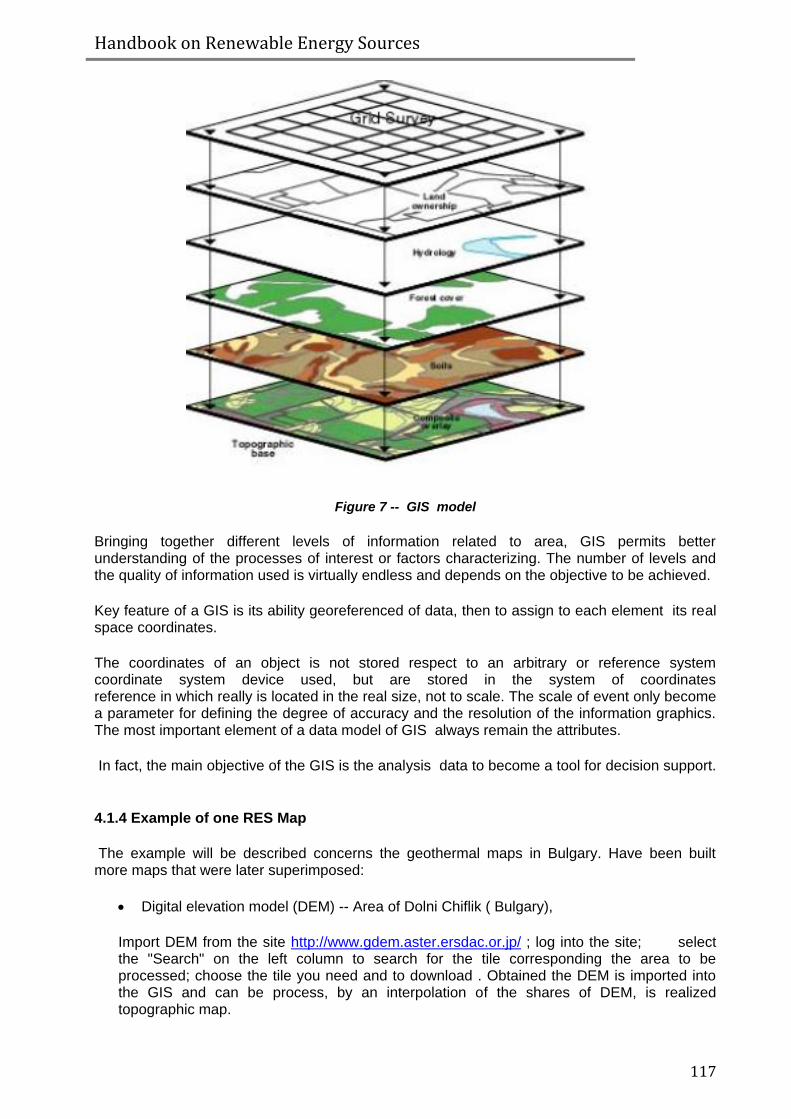
Handbook on Renewable Energy Sources
117
Figure 7 -- GIS model
Bringing together different levels of information related to area, GIS permits better understanding of the processes of interest or factors characterizing. The number of levels and the quality of information used is virtually endless and depends on the objective to be achieved.
Key feature of a GIS is its ability georeferenced of data, then to assign to each element its real space coordinates.
The coordinates of an object is not stored respect to an arbitrary or reference system coordinate system device used, but are stored in the system of coordinates reference in which really is located in the real size, not to scale. The scale of event only become a parameter for defining the degree of accuracy and the resolution of the information graphics. The most important element of a data model of GIS always remain the attributes.
In fact, the main objective of the GIS is the analysis data to become a tool for decision support.
4.1.4 Example of one RES Map
The example will be described concerns the geothermal maps in Bulgary. Have been built more maps that were later superimposed:
Digital elevation model (DEM) -- Area of Dolni Chiflik ( Bulgary),
Import DEM from the site http://www.gdem.aster.ersdac.or.jp/ ; log into the site; select the "Search" on the left column to search for the tile corresponding the area to be processed; choose the tile you need and to download . Obtained the DEM is imported into the GIS and can be process, by an interpolation of the shares of DEM, is realized topographic map.
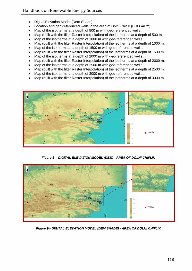
Handbook on Renewable Energy Sources
118
Digital Elevation Model (Dem Shade).
Location and geo-referenced wells in the area of Dolni Chiflik (BULGARY).
Map of the isotherms at a depth of 500 m with geo-referenced wells.
Map (built with the filter Raster Interpolation) of the isotherms at a depth of 500 m.
Map of the isotherms at a depth of 1000 m with geo-referenced wells .
Map (built with the filter Raster Interpolation) of the isotherms at a depth of 1000 m.
Map of the isotherms at a depth of 1500 m with geo-referenced wells.
Map (built with the filter Raster Interpolation) of the isotherms at a depth of 1500 m.
Map of the isotherms at a depth of 2000 m with geo-referenced wells .
Map (built with the filter Raster Interpolation) of the isotherms at a depth of 2000 m.
Map of the isotherms at a depth of 2500 m with geo-referenced wells .
Map (built with the filter Raster Interpolation) of the isotherms at a depth of 2500 m.
Map of the isotherms at a depth of 3000 m with geo-referenced wells .
Map (built with the filter Raster Interpolation) of the isotherms at a depth of 3000 m.
Figure 8 -- DIGITAL ELEVATION MODEL (DEM) - AREA OF DOLNI CHIFLIK
Figure 9-- DIGITAL ELEVATION MODEL (DEM SHADE) - AREA OF DOLNI CHIFLIK

Handbook on Renewable Energy Sources
119
Figure 10-- LOCATION WELLS IN THE NORTH-EAST OF BULGARY
Figure 11-- LOCATION WELLS IN THE AREA OF DOLNI CHIFLIK

Handbook on Renewable Energy Sources
120
Figure 12-- MAP OF THE ISOTHERMS AT A DEPTH OF 500
Figure 13- MAP (built with the filter Raster Interpolation) OF THE ISOTHERMS AT A DEPTH OF 500 m
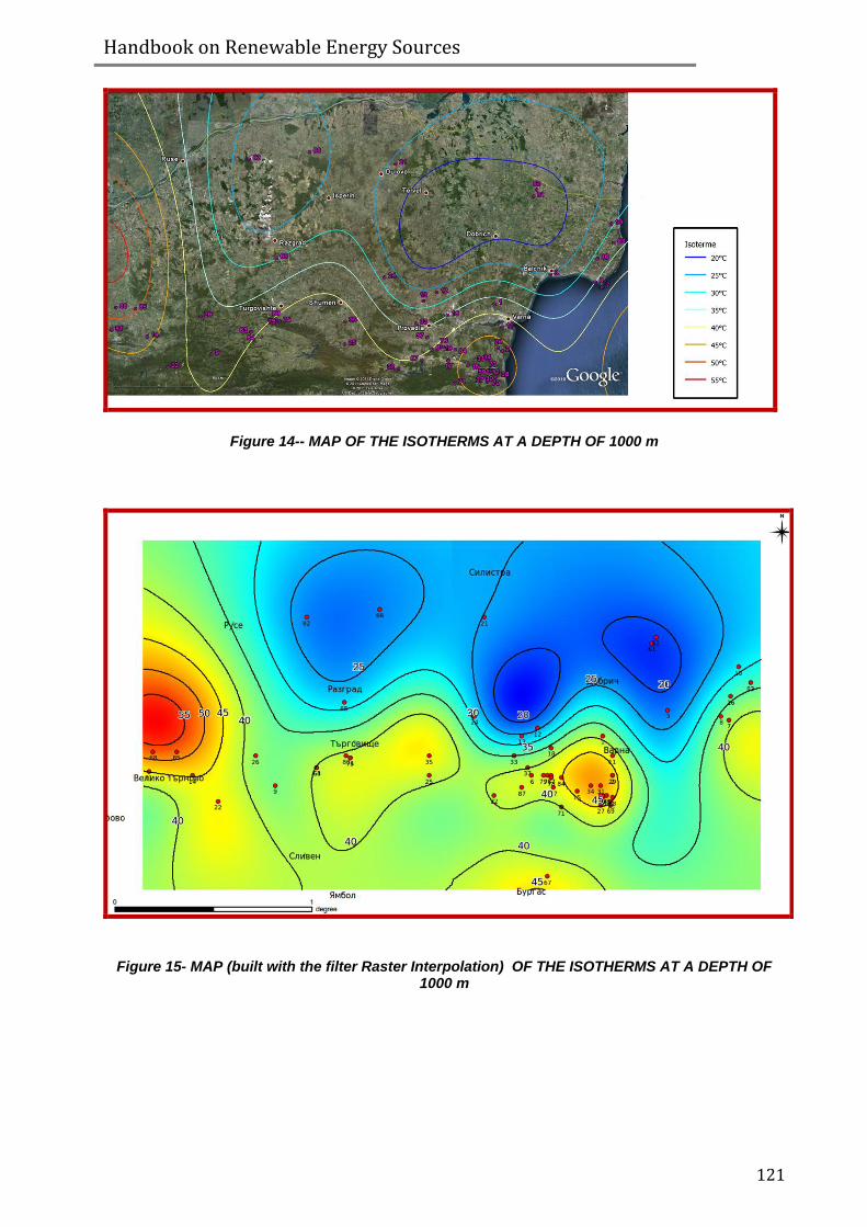
Handbook on Renewable Energy Sources
121
Figure 14-- MAP OF THE ISOTHERMS AT A DEPTH OF 1000 m
Figure 15- MAP (built with the filter Raster Interpolation) OF THE ISOTHERMS AT A DEPTH OF 1000 m

Handbook on Renewable Energy Sources
122
Figure 16-- MAP OF THE ISOTHERMS AT A DEPTH OF 1500 m
Figure 17- MAP (built with the filter Raster Interpolation) OF THE ISOTHERMS AT A DEPTH OF 1500 m

Handbook on Renewable Energy Sources
123
Figure 18-- MAP OF THE ISOTHERMS AT A DEPTH OF 2000 m
Figure 19- MAP (built with the filter Raster Interpolation) OF THE ISOTHERMS AT A DEPTH OF 2000

Handbook on Renewable Energy Sources
124
Figure 20-- MAP OF THE ISOTHERMS AT A DEPTH OF 2500 m
Figure 21- MAP (built with the filter Raster Interpolation) OF THE ISOTHERMS AT A DEPTH OF 2500 m

Handbook on Renewable Energy Sources
125
Figure 22-- MAP OF THE ISOTHERMS AT A DEPTH OF 3000 m
Figure 23- MAP (built with the filter Raster Interpolation) OF THE ISOTHERMS AT A DEPTH OF 3000 m
The representation of these maps facilitates the identification of potentially interesting areas for the development of geothermal energy and the immediate choice between the existing wells in areas where the isotherms have a higher temperature.

Handbook on Renewable Energy Sources
126
INDEX
Biomass
GJ Gigajoule – unit of energy corresponding to 109 Joules
PJ Petajoule – unit of energy corresponding to 1015
Joules
kWe Kilowatt electrical – unit of electrical power equivalent to 103 Watts
kWth Kilowatt thermal – unit of thermal power equivalent to 103 Watts
CO2 Carbon dioxide
CO2e
Carbon dioxide greenhouse gas equivalent represent the emissions quantity of all GHG gases compared, in the earth warming effects, to the CO2 gas taking in consideration the conversion values. The Methane effect for the warming earth is comparable to 21 times respect to CO2, while N20 is equivalent to 310 times respect to CO2.
N2O Nitrous Oxide is a greenhouse gas released by the bacterial breakdown of soil nitrogen and during the combustion
Alcohol Hydrocarbons with an –OH group attached to the carbon chain
Anaerobic Digestion
Biological degradation via microorganisms of carbonaceous material, mainly in the absence of oxygen to methane (CH4) and hydrogen (H2) and small quantities CO2, H2S
Biochar Black carbonaceous solid resulting from the pyrolysis of biomass
Bioenergy Technically any thermal or electrical energy sourced from the conversion of biomass
Biofuel Technically any biologically derived solid, liquid or gaseous fuel for combustion applications, but sometimes limited to transport fuels
Calorific Value Calorific value refers to the amount of energy released during the combustion of a fuel
Carbohydrates Molecules usually of biological origin consisting of carbon, hydrogen and oxygen
Carbon Sequestration
The capture and medium-to-long term storage of atmospheric carbon (primarily carbon dioxide) into carbon 'sinks' such as forests, soil, oceans and geological formations
Cellulose An insoluble crystalline polymer of glucose and largest bulk molecular component of plants. See Lignocellulose and Carbohydrates
Climate Change Variation in mean global temperature as a result of anthropogenic activities, also referred to as global warming
Cogeneration A generating facility that produces, in the same time, electricity and thermal energy
Combustion Complete oxidation of fuel
Coppice Trees or shrubs that are cut for re-growth at regular intervals
Fermentation Biological degradation of soluble sugars to ethanol or butanol and CO2 by microorganisms in the absence of oxygen
Gasification Heating and partial oxidation of carbonaceous material to produce ‘syngas’
Greenhouse Gases
Gaseous emissions that contribute to global warming. They include carbon dioxide (CO2), methane (CH4=25 CO2e), nitrous oxide (N2O=296 CO2e) and other gases generated during industrial processes
Hydrocarbons Molecules consisting of carbon and hydrogen arranged in a chain, branching or ring structure; the basis of liquid transport fuels

Handbook on Renewable Energy Sources
127
Lignin An amorphous matrix molecule in plants containing linked aromatic rings. See Lignocellulose
Lignocellulose An insoluble carbohydrate found in plant cell walls and therefore making up the majority of plant derived biomass. It comprises cellulose and fibres within a lignin matrix, with some hemicellulose to aid in bonding
Pyrolysis Heating carbonaceous material in the absence of oxygen to produce char, oil and gas outputs
Pyrolysis Oil Complex mixture of highly oxygenated hydrocarbons resulting from the thermal
depolymerisation of biomass in the absence of oxygen
Syngas A mixture of Hydrogen (H2) and Carbon Monoxide (CO) produced by gasification that can be combusted or used as chemical feedstock for synthesis reactions
Watt (W):
Unit of power equivalent to 1 Joule of energy use per second
Hydropower
Alternating current (AC)
electric current that reverses its polarity periodically (in contrast to direct current). In Europe the standard cycle frequency is 50 Hz, in N. and S. America 60 Hz
Anadromous fish fish (e.g. salmon) which ascend rivers from the sea at certain seasons to spawn Average Daily Flow the average daily quantity of water passing a specified gauging station
Baseflow that part of the discharge of a river contributed by groundwater flowing slowly through the soil and emerging into the river through the banks and bed
BFI baseflow index the proportion of run-off that baseflow contributes
Butterfly Valve a disc type water control valve, wholly enclosed in a circular pipe, that may be opened and closed by an external lever. Often operated by a hydraulic system
Capacitor a dielectric device which momentarily absorbs and stores electric energy
Catchment Area
the whole of the land and water surface area contributing to the discharge at a particular point on a watercourse
Cavitation a hydraulic phenomenon whereby liquid gasifies at low pressure and the vapour bubbles form and collapse virtually instantaneously causing hydraulic shock to the containing structure. This can lead to severe physical damage in some cases
Compensation flow
the minimum flow legally required to be released to the watercourse below an intake, dam or weir, to ensure adequate flow downstream for environmental, abstraction or fisheries purposes
Demand (Electric) the instantaneous requirement for power on an electric system (kW or MW)
Demand Charge
that portion of the charge for electric supply based upon the customer’s demand characteristics
Direct Current (DC) electricity that flows continuously in one direction sd contrasted with alternating current
Draft tube a tube full of water extending from below the turbine to below the minimum water tailrace level

Handbook on Renewable Energy Sources
128
Energy work, measured in Newton metres or Joules. The electrical energy term generally used is kilowatt-hours (kWh) and represents power (kilowatts) operating for some period of time (hours) 1 kWh = 3.6x10
3 Joules
Evapotranspiration the combined effect of evaporation and transpiration
FDC flow duration curve: a graph of discharges against v. the percentage of time (of the period of record) during which particular magnitudes of discharge were equalled or exceeded
Fish Ladder a structure consisting e.g. of a series of overflow weirs which are arranged in steps that rise about 30 cm in 3 50 4 m horizontally, and serve as a means for allowing migrant fish to travel upstream past a dam or weir
Output the amount of power (or energy, depending on definition) delivered by a piece of equipment, station or system
(In) Parallel the term used to signify that a generating unit is working in connection with the mains supply, and hence operating synchronously at the same frequency
Overspeed the speed of the runner when, under design conditions, all external loads are removed
P.E. polyethylene
Peak Load the electric load at the time of maximum demand
Peaking Plant a powerplant which generates principally during the maximum demand periods of an electrical supply network
Penstock a pipe (usually of steel, concrete or cast iron and occasionally plastic) that conveys water under pressure from the forebay to the turbine
Percolation the movement of water downwards through the soil particles to the phreatic surface (surface of saturation within the soil; also called the groundwater level)
Power the capacity to perform work. Measured in joules/sec or watts (1MW = 1 j/s). Electrical power is measured in kW
Power factor the ratio of the amount of power, measured in kilowatts (kW) to the apparent power measured in kilovolt-amperes (kVA)
Rating curve the correlation between stage and discharge
Reynolds Number
a dimensionless parameter used in pipe friction calculations (interalia), and derived from pipe diameter, liquid velocity and kinematic viscosity
Rip-rap stone, broken rock or concrete block revetment materials placed randomly in layers as protection from erosion
Runoff the rainfall which actually does enter the stream as either surface or subsurface flow
Run-of-river scheme plants where water is used at a rate no greater than that with which it “runs” down the
river
SOIL a parameter of permeability
Stage (of a river)
the elevation of water surface
Supercritical flow
rapid flow who is unaffected by conditions downstream

Handbook on Renewable Energy Sources
129
Synchronous speed the rotational speed of the generator such that the frequency of the alternating current
is precisely the same as that of the system being supplied
Tailrace the discharge channel from a turbine before joining the main river channel
Wind
Aerofoil Shape of a cross-section of a rotor blade
Angle of attack Angle between the resultant (or relative) wind velocity and the chord line of a blade section
Aspect ratio (AR): Ratio of the rotor blade radius R to the average blade chord length c
(large aspect ratio: 1Rc
Capital cost
The capacity factor is defined as the wind turbine’s annual electricity yield (in kWh) divided by the electricity output if the turbine would have operated at its rated power output for the entire year (i.e. the installed power times 365 days times 24 hours). Reasonable capacity factors range from 0.25 to 0.30, while a very good capacity factor would be 0.40
Capacity factor The capital cost include the purchase price, cost of transporting, assembling, and erecting a wind turbine on site, as well as the cost of installing grid lines and connecting the turbine to the grid
Capital cost Width of a cross-section of a rotor blade, i.e. local dimension perpendicular to the blade radius R.
Chord (c): Gusts of wind with dimensions larger than the rotor swept area, see non-coherent gusts.
Coherent gusts Device of which the dynamics interact with the dynamics of a physical system (e.g. a wind turbine), and so have implications for the obtained performance.
Control system Damping is the dissipation of energy with time or distance.
Damping
The number of degrees of freedom of a mechanical system is equal to the minimum number of independent coordinates required to define completely the positions of all parts of the system at any instant of time. In general, it is equal to the number of independent displacements that are possible
Degrees of freedom Used to indicate that the rotor is placed at the back of the tower as seen from the main wind direction, cf. upwind
Downwind Part of a wind turbine consisting of the rotor shaft, rotor inertia, transmission, and generator
Drive-train
Dynamic stall or stall hysteresis is a dynamic effect which occurs on aerofoils if the angle of attack changes more rapidly than the air flow around the blade (or blade element) can adjust to. The result is aerofoil lift and drag coefficients which depend not only on the instantaneous angle of attack (quasi-steady aerodynamics assumption), but also on the recent angle of attack history
Dynamic stall
A prismatic beam with length L, cross-section area A = π·R2, constant
flexural rigidity EI, and uniformly distributed mass per unit length ρ = m/L, where m is the total mass of the beam. It is assumed that both the shear deformation and rotational inertia of the cross-sections are negligible if compared with bending
Euler-Bernoulli beam deformation and translational inertia, respectively. This assumption leads to a good approximation if the beam is very slender (i.e. R << L).
External cost: Cost associated with damage to the environment and health with are not included in the electricity price, for example the cost due to greenhouse gas emissions which may cause global warming
Extreme loads Highest loads that are likely to be experienced by a wind turbine within its life-time (i.e. extreme operating conditions).
Fatigue loads Dynamic loads that are experienced by a wind turbine repeatedly during its life-time (i.e. normal operating conditions).
Flap motion Out-of-plane (elastic) bending of the blade, i.e. normal to the plane of

Handbook on Renewable Energy Sources
130
rotation (cf. lead-lag motion).
Flexible body
A body in a system has to be treated as flexible when the rigid body assumption is not valid. In other words: the deformation of the body has a significant effect on the dynamic behaviour of the system, cf. rigid body
Generator Device which converts mechanical power into electrical power Horizontal-axis wind turbine
Wind turbine of which the rotor shaft is substantially parallel to the wind flow, cf. vertical-axis wind turbine
Hub Fixture for attaching the blades or blade assembly to the rotor shaft
Hub height (H): Height of the centre of the horizontal-axis wind turbine rotor above the terrain surface.
Infinite bus Voltage source of constant voltage and frequency
Kinematics The study of the geometry of motion. Kinematics is used to relate displacement, velocity, acceleration, and time without reference to the cause of the motion.
Lead-lag motion In-plane (elastic) bending of the blade, cf. flap motion.
Leakage
Leakage is a problem which is a direct consequence of the fact that the Fast Fourier Transform (FFT) assumes that the discrete set of N point comes from a trigonometric polynomial of frequencies that are multiples of the sample frequency, namely fs = 1/T. Thus the FFT assumes that the finite record of length T is periodic over the sampling interval chosen with period T. In general this will not be true, and leads to a problem known as leakage. Leakage leads to an overestimate of the damping. Leakage can be corrected to some degree by the use of a window function (e.g. Hanning window or Exponential window) which forces the signal to damp at the end of the time record. But windowing adds its own damping, causing additional leakage. Nevertheless, it is recommended that a window should always be used except when the signal is truly periodic in time, or the signal is a transient which has died away within the record length.
Load: Force or moment on a component (or section of a component) of a wind turbine
Multibody system An approximation of a real mechanical system by a series of interconnected rigid and flexible bodies
Nacelle
Housing which contains the stationary part of the generator (or: stator), and the ground plate at which the yaw mechanism has been placed. The nacelle mass equals the sum of the mass of the chassis (including yaw motor, yaw bearing, flanges et cetera) and the generator stator mass
Non-coherent gusts Gusts of wind with dimensions smaller than the rotor swept area, see coherent gusts
Operation and maintenance (O&M) costs
They include all ttroubleshooting, inspections, adjustments, retrofits, preventive, as well as unscheduled maintenance performed on wind turbines, and the downtime that accumulates while waiting for parts, instructions, or outside services that are not available on site but are required to bring the turbine back in operation.
Particle
The most simple approximation of (an element of) a system is a free particle (or point mass). A particle is assumed to have no dimensions and accordingly can be treated as point in the three-dimensional space. In other words: it is assumed that the mass could be concentrated in one point, and that all forces act at that point (i.e. rotation about the mass center is neglected).
Pitch-flap flutter
Pitch-flap flutter is defined as the combined bending and torsional vibration of a rotor blade in steady air flow. It arises when the inertia axis (locus of the mass centres of the cross-sections along the blade) does not coincide with the elastic axis (locus of the shear centres, where a shear centre is a point such that a shearing force passes through it produces pure bending and a moment about it produces pure torsion). Note that if the cross-section is symmetric, the shear centre coincides with the mass centre of the cross-section (assuming that the mass centre is identical with the area centre of the cross-section).

Handbook on Renewable Energy Sources
131
Point mass see particle
Power electronics The task of power electronics is to process and control the flow of electric energy by supplying voltages and currents in a form that is optimally suited for user loads.
Reynolds number (Re):
The Reynolds number is a dimensionless number that determines whether the flow around a wind turbine rotor blade (or blade element) is
laminar or turbulent, and is defined as: Re = (W.c)/ν, where W is the relative wind velocity, c the local chord, and ν the kinematic viscosity. The kinematic viscosity is, in turn, defined as ν = ρ/μ, where ρ the density of air, and μ the dynamic viscosity. The Reynolds number can be interpreted as the ratio of inertial to viscous forces acting on the air
flow. For air at standard, sea-level conditions, Re = 69000 W.c. It is important to stress that aerofoil data used in rotor modelling must be near the correct Reynolds number, because otherwise accurate results cannot be expected
Rigid body
A body in a system can be treated as rigid when the deformation is too small, such that it can be neglected. For a rigid body, the distance between any two points on the body remains constant, and accordingly the kinematics of the rigid body is the same as the kinematics of its reference. The dynamic motion of a rigid body is described by a set of ordinary differential equations, see flexible body.
Rotational sampling The phenomenon that air vortices, with dimensions smaller than the rotor swept area, are locally hit during each cycle by the rotation of the wind turbine blades.
Solidity The ratio of the total blade area to the swept area, see swept area.
Super-element
A super-element is a multibody approximation of a (part of a) flexible body consisting of three (describing bending only) or four (describing bending, axial deflection, and torsion) rigid bodies connected by ideal springs, and dampers
Stall Reduction of lift (or change in pitching moment or decrease in drag) associated with separation of airflow from the surface of the rotor blade.
Stall hysteresis see dynamic stall
Stiffness: Stiffness is the ratio of change of force (or torque) to the corresponding change on translational (or rotational) deflection of an elastic element.
Support structure Part of a wind turbine comprising the tower (up to the yaw bearing) and the foundation.
Swept area (A): Area of the projection, upon a plane perpendicular to the wind velocity vector, of the disc along which the rotor blade tips move during rotation.
Theoretical modelling In theoretical or fundamental modelling the relevant physical properties of the system are derived from first principles (e.g. conservation laws).
Tip loss Loss of lift relative to 2-D aerodynamic profile data at the blade tip due to three-dimensional induced effects.
Total harmonic distortion (THD):
Current or voltage THD is the root-sum-square of the harmonic components divided by the fundamental component.
Twist Twist is applied to maintain the optimum angle of attack α, and hence
the maximum lift coefficient maxlC , constant along the rotor blade.
Unsteady aerodynamics Wind turbines operate at all times in an unsteady environment. Two main areas can be discriminated: dynamic inflow and dynamic stall.
Upwind Used to indicate that the rotor is placed in front of the tower as seen from the main wind direction, cf. downwind.
Validation The process of determining whether or not the verified mathematical model of a system behaves similar to the real behaviour associated with the intended model use.
Verification The process of determining whether or not a computer simulation model is consistent with the underlying mathematical model to a specified accuracy level.
Vertical-axis wind turbine:
Wind turbine of which the rotor shaft is vertical, cf. horizontal-axis wind turbine.
Wind Energy Conversion System (WECS): see wind turbine

Handbook on Renewable Energy Sources
132
Windmill
System that converts kinetic energy in the wind into mechanical energy. The mechanical energy is typically used for grain-grinding, pumping water, and sawing wood. The term “windmill” comes from the fact that to “mill” means to grind.
Wind turbine see wind turbine.
Wind Turbine Generator (WTG):
System that converts kinetic energy in the wind into electrical energy. Note that “turbine” in the definition of wind turbine is used as pars pro toto for the whole structure (i.e. from the rotor blades to foundation).
Aerodynamic notation
Axial induction factor [–]
α΄ Tangential induction factor (represents induced swirl) [–]
A = πR2 Rotor swept area, or equivalently actuator disk area [m
2]
AR Aspect ratio of blade, R/c0.75 [–]
(i.e. based at chord length at 75% radius)
c Local blade chord [m]
Cd Blade element drag coefficient [–]
Cdax Thrust coefficient [–]
Cl Blade element lift coefficient [–]
Cm Blade element moment coefficient [–]
Cp Power coefficient [–]
Ct Thrust coefficient [–]
D Rotor diameter [m]
D Drag force [N]
Dax Rotor thrust or axial force on rotor [N]
F Force [N]
Faero Aerodynamic forces [N]
FL Effective total loss factor [–]
Froot Prandtl root-loss factor [–]
Ftip Prandtl tip-loss factor [–]
H Hub height [m]
wV
υα

Handbook on Renewable Energy Sources
133
L Length [m]
L Lift force [N]
M Pitching moment [Nm]
Ma Mach number [–]
Nb Number of rotor blades [–]
Ns Number of blade elements [–]
p0 Static pressure [N/m2]
P Power extracted from the wind [W]
q Dynamic pressure [N/m2]
r Radius of rotor blade section (i.e. local radius) [m]
Rotor radius [m]
Re Reynolds number [–]
S Cross-sectional area of cylindrical control volume [m2]
υ Axial induced wind velocity [m/s]
Vax Wind velocity at rotor disk position [m/s]
Vp Local, undisturbed, perpendicular wind velocity [m/s]
Vr Rated wind velocity [m/s]
Vt Local, undisturbed, tangential wind velocity [m/s]
Vw Undisturbed wind velocity [m/s]
V∞ Wind velocity in the turbine wake [m/s]
W Local, undisturbed, aerodynamic wind velocity [m/s]
ẋ Velocity [m/s]
α Angle of attack of aerodynamic velocity [deg]
ΔD Element drag force [N]
ΔF Axial components of aerodynamic forces [N]
ΔL Element lift force [N]
ΔQ Tangential components of aerodynamic forces [N]
Δr Small section of rotor blade [m]
DR2
1
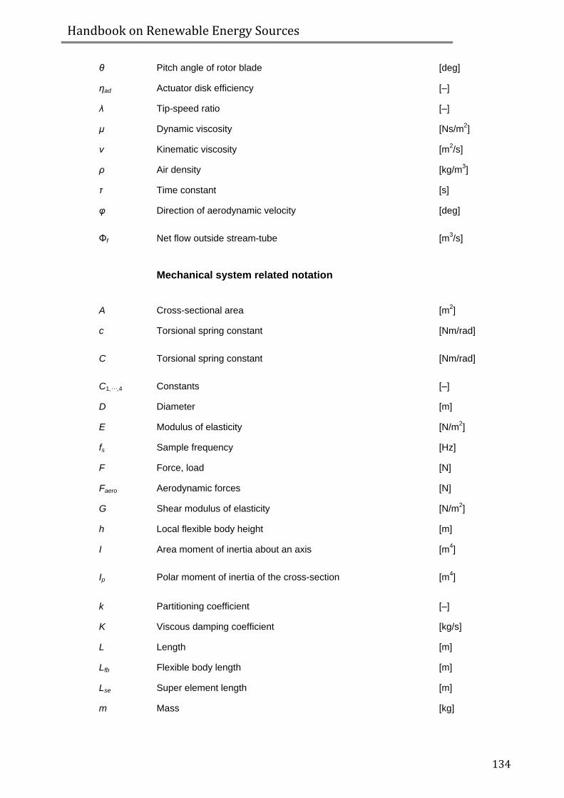
Handbook on Renewable Energy Sources
134
θ Pitch angle of rotor blade [deg]
ηad Actuator disk efficiency [–]
λ Tip-speed ratio [–]
μ Dynamic viscosity [Ns/m2]
ν Kinematic viscosity [m2/s]
ρ Air density [kg/m3]
τ Time constant [s]
φ Direction of aerodynamic velocity [deg]
Φf Net flow outside stream-tube [m3/s]
Mechanical system related notation
A Cross-sectional area [m2]
c Torsional spring constant [Nm/rad]
C Torsional spring constant [Nm/rad]
C1,···,4 Constants [–]
D Diameter [m]
E Modulus of elasticity [N/m2]
fs Sample frequency [Hz]
F Force, load [N]
Faero Aerodynamic forces [N]
G Shear modulus of elasticity [N/m2]
h Local flexible body height [m]
I Area moment of inertia about an axis [m4]
Ip Polar moment of inertia of the cross-section [m4]
k Partitioning coefficient [–]
K Viscous damping coefficient [kg/s]
L Length [m]
Lfb Flexible body length [m]
Lse Super element length [m]
m Mass [kg]
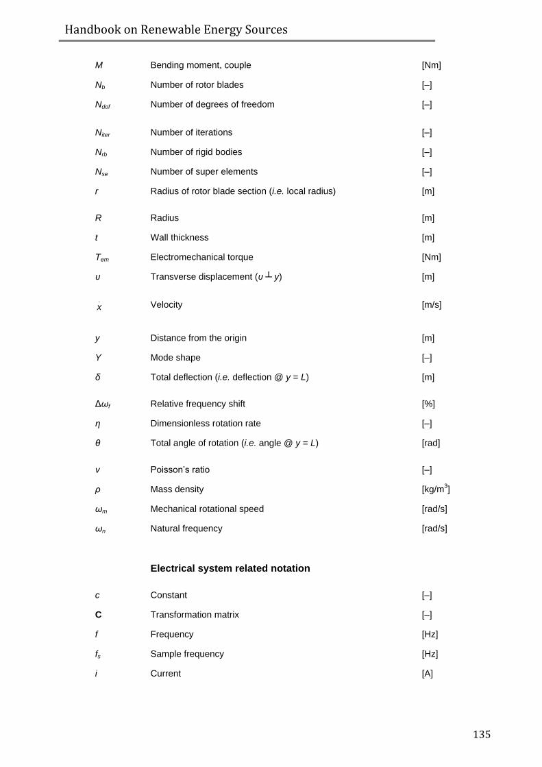
Handbook on Renewable Energy Sources
135
M Bending moment, couple [Nm]
Nb Number of rotor blades [–]
Ndof Number of degrees of freedom [–]
Niter Number of iterations [–]
Nrb Number of rigid bodies [–]
Nse Number of super elements [–]
r Radius of rotor blade section (i.e. local radius) [m]
R Radius [m]
t Wall thickness [m]
Tem Electromechanical torque [Nm]
υ Transverse displacement (υ ┴ y) [m]
Velocity [m/s]
y Distance from the origin [m]
Y Mode shape [–]
δ Total deflection (i.e. deflection @ y = L) [m]
Δωf Relative frequency shift [%]
η Dimensionless rotation rate [–]
θ Total angle of rotation (i.e. angle @ y = L) [rad]
ν Poisson’s ratio [–]
ρ Mass density [kg/m3]
ωm Mechanical rotational speed [rad/s]
ωn Natural frequency [rad/s]
Electrical system related notation
c Constant [–]
C Transformation matrix [–]
f Frequency [Hz]
fs Sample frequency [Hz]
i Current [A]
.
x

Handbook on Renewable Energy Sources
136
i α, i b & i c Stator current of the a-phase, b-phase, and c-phase [A]
i d Direct-axis current [A]
i f Field-winding current [A]
i q Quadrature-axis current [A]
L Inductance (H=kg·m2/(A
2·s
2)) [H]
L Inductance matrix [H]
Ld Direct-axis synchronous inductance [H]
L0 Zero-sequence inductance [H]
Lq Quadrature-axis synchronous inductance [H]
Lrr Rotor self-inductance matrix [H]
Lss Stator self-inductance matrix [H]
Mrs Rotor-stator mutual inductance matrix [H]
Msr Stator-rotor mutual inductance matrix [H]
n Rotor speed [r.p.m.]
p Number of pole-pairs [–]
Pelec Electrical power [W]
R Initial magnetic state []
R Resistance matrix [Ω]
R α, Rb & Rc
Stator resistance of the a-phase, b-phase, and c-phase [Ω]
R1d Direct-axis damper resistance [Ω]
Rf Field-winding resistance [Ω]
R1q Quadrature-axis damper resistance [Ω]
Rs Stator-winding resistance [Ω]
S Switch [0,1]
t Time [s]
T0dq Park’s power-invariant transformation matrix [–]
Tem Electromechanical torque [Nm]

Handbook on Renewable Energy Sources
137
ua, ub & uc Stator voltage of the a-phase, b-phase, and c-phase [V]
ud Direct-axis voltage [V]
u1d Direct-axis damper winding voltage [V]
uf Field-winding voltage [V]
uq Quadrature-axis voltage [V]
u1q Quadrature-axis damper winding voltage [V]
Udc DC link voltage [V]
єα Current error of phase a [A]
ηconv Frequency converter efficiency [–]
θe Angle between the direct-axis and the magnetic axis
of phase a [deg]
ψα, ψb & ψc
Stator flux linkages of the a, b, and c-phase [Vs]
ψd Direct-axis stator flux [Vs]
ψ1d Direct-axis damper flux [Vs]
ψf Direct-axis field winding flux [Vs]
ψq Quadrature-axis stator flux [Vs]
ψ1q Quadrature-axis damper flux [Vs]
ωm Mechanical rotational speed [rad/s]
Δi Width hysteresis band [A]
Waves related notation (for offshore wind)
d Water depth [m]
D Cross-section dimension [m]
g Gravity constant [m/s2]
H Wave height [m]
L Wave length [m]
T Wave period [s]

Handbook on Renewable Energy Sources
138
Control system related notation
C Controller
e Error signal
F Filter
L Loop gain
P Rotor power
Pci Start power
Pr Rated aerodynamic power
r Reference signal
P Rotor power
Pci Start power
Pr Rated aerodynamic power
r Reference signal
S Sensitivity function of the closed-loop system
T Complementary sensitivity function of the closed-loop system
u Input signal
υ Disturbance
Vci Cut-in wind velocity
Vco Cut-out wind velocity
Vr Rated wind velocity
Vw Undisturbed wind velocity
y Measured output
λ Tip-speed ratio
Special (e.g. arithmetic) symbols
j Imaginary number
J Mass moment of inertia
k Viscous damper coefficient
IR Set of real numbers
t Time
T Kinetic energy

Handbook on Renewable Energy Sources
139
U Potential energy
Δ Deviation
Π Parametrization, mapping
∇ Gradient vector
∇2 ∂
2∕∂x
2+∂
2∕∂y
2+∂
2∕∂z
2
|| · || Euclidian norm
Geothermal
Acid Rain
common name for any precipitation (rain, snow, sleet, hail, fog) having a high amount of sulfuric acid and/or nitric acid or having a pH lower than 5.6. Normal rain has a pH of 5.6 - 5.7. Accumulation of acids in lakes and rivers damages or kills plant and animal life. Acid rain also dissolves building materials and leaches nutrients out of soil resulting in crop damage. Fossil fuel power plants are a major source of acid rain
Agriculture
the growing (farming) of plants, flowers, trees, grains, and other crops. Greenhouses can be heated with hot water from geothermal reservoirs. In some places pipes of hot water are buried under the soil. Geothermal heat is also used to dry crops
Aquaculture the farming of fish and other water-dwelling organisms in freshwater or seawater. Geothermal water is used to help speed the growth of fish, prawns and alligators. China is probably has more aquaculture operations than any other country
Aquifer a large permeable body of underground rock capable of yielding quantities of water to springs or wells. Aquifers provide about 60 percent of American drinking water. Underground aquifers of hot water and steam are called geothermal reservoirs
Balneology using hot spring mineral water for therapy. This is perhaps the oldest use of natural geothermal waters
Boiling point
temperature at which a single substance, such as water, changes from a liquid to a gas (steam) under normal atmospheric pressure. The boiling point at which water transitions to steam is 212°F (100°C). Some liquids boil at a lower temperature than water -- a principle utilized in binary power plants. Boiling point is also affected by pressure. The greater the pressure, the higher the boiling point. This principle is put to work in geothermal (flash) power plants when superheated (hotter than boiling) geothermal water is brought up wells. The hot water flashes to steam when the pressure is released as it reaches the surface. This phenomenon also occurs naturally, resulting in such features as geysers
Caldera a bowl-shaped landform, created either by a huge volcanic explosion (which destroys the top of a volcano) or by the collapse of a volcano's top
Carbon dioxide (CO2)
a gas produced by the combustion of fossil fuels and other substances. CO2 also occurs naturally in large amounts in molten magma, which is involved in the explosive eruption of volcanoes. See Greenhouse Effect
Chemical energy
: energy inherent in the chemical bonds which hold molecules together. Examples are coal and oil, which have energy potential that is released upon combustion
Combustion the burning of gas, liquid, or solid, in which the fuel is oxidized, producing heat and often light
Condense
to change from a gas to drops of liquid. Water-cooled geothermal power plants use cooling towers to cool the used steam and condense it back to water for injection back to the edge of the reservoir. In binary power plants, an organic liquid is first vaporized (with heat from geothermal water) to drive a turbine, then cooled and condensed back to a liquid and recycled again and again in a closed loop

Handbook on Renewable Energy Sources
140
Conduction
the transfer of heat as a result of the direct contact of rapidly moving molecules through a medium or from one medium to another, without movement of the media. The heat from geothermal water, for instance can be conducted through metal plates or pipes to heat other water for district heating systems or a second organic liquid for use in binary power plants
Continental drift
the theory that the continents have drifted apart when a supercontinent, Pangaea, broke apart. See Plate Tectonics
Convection currents
the currents caused by hot air or fluid rising and falling. Hot air or fluid expands and is therefore less dense than its cooler surroundings, thus it rises; as it cools it contracts, becomes more dense and sinks down creating something of a rolling motion. These motions are thought to be party of the dynamic geologic processes that drive the movement of crustal plates. See Plate Tectonics
Core (outer and inner)
the extremely hot center of the Earth. The outer core is probably molten rock and is located about 3,200 miles (5,100) kilometers down from the earth’s surface; the inner core may be solid iron and is found a the very center of the Earth- about 4,000 miles (6,400 kilometers) down
Crust the solid outermost layer of the Earth, mostly consisting of rock, and ranging from 3 - 35 miles (4.8 - 56 kilometers) thick, comprises the topmost portion of the lithosphere (see lithospheric plates). Earth's crust insulates us from the hot interior
Cultivate to grow and tend (plants or crops), farm
Dehydrate to free from moisture in order to preserve; to dry fruits, vegetables or lumber, for instance. A factory in in Nevada, for example uses geothermal heat to dehydrate onions and garlic for restaurants
Density
the amount of mass in a given volume of something. Two objects can be the same size, but have different densities because one of the objects has more mass "packed" into the same amount of space. Objects are smaller when they are cold, larger when hot
Direct use use of geothermal water and it's heat to grow fish, dry vegetable, fruit and wood products, heat greenhouses and city buildings, or provide hot water for spas
District heating system
: a heating system that provides heat to a large number of buildings all from a central facility. In geothermal district heating systems, one or more wells can serve entire districts
Earthquake the vibration or movement of the ground caused by a sudden shift along faults (cracks) in the earth's crust; most earthquakes occur at the places where tectonic plates edges meet
Electric current
the continuous flow of electrons; often referred to as electricity
Electrical energy
energy of electric charges or electric currents
Electron the smallest part of an atom (atoms are the tiny particles of which all substances are made). Electrons may be freed from atoms to produce an electric current
Energy conversion
the changing of energy from one form to another. One of the many examples are heat energy being converted into mechanical energy, and then mechanical energy into electrical energy, as is done in steam-driven electric power plants
Energy efficiency
the measure of the amount of energy which any technology can convert to useful work; technology with a higher energy efficiency will require less energy to do the same amount of work
Energy resource
a source of useable power which can be drawn on when needed. Energy resources are often classified as renewable or non-renewable
Energy the ability to do work, such as making things move and heating them up. Energy can take many forms, including electrical, chemical, radiant, mechanical and heat
Environmental Protection Agency (EPA)
Federal government agency that makes and enforces standards for pollution control; designed to protect the environment
Eruption the explosive discharge of material such as molten rock and gases, or hot water

Handbook on Renewable Energy Sources
141
(as from volcanoes or geysers).
Fault a crack or break in the Earth’s crust along which movement has occurred, often resulting in earthquakes
Fracture a crack in the Earth’s crust along which no movement has occurred
Fumarole a small hole or vent in the Earth's surface, found near volcanic areas, from which steam or gases shoot out
Generator a machine that converts mechanical power into electricity by spinning copper wires (conductors) within a magnetic field
Geothermal (ground source) heat pump
a space heating/cooling system which moves heat from and to the earth, as opposed to making heat using a fuel source. Geothermal heat pumps take advantage of the almost constant temperature just a few feet underground -- usually warmer than the air in winter and cooler than the air in summer
Geothermal reservoir
a large volume of underground hot water and steam in porous and fractured hot rock. The hot water in geothermal reservoirs occupies only 2 to 5% of the volume of rock, but if the reservoir is large enough and hot enough, it can be a powerful source of energy. Geothermal reservoirs are sometimes overlain by a layer of impermeable rock. While geothermal reservoirs usually have surface manifestations such as hot springs or fumaroles, some do not
Geothermal phenomena
an observable event at the surface, whose occurrence is the result of the Earth’s internal heat; includes volcanoes, geysers, hot springs, mud pots and fumaroles
Geothermal power plant
a facility which uses geothermal steam or heat to drive turbine-generators to produce electricity. Three different types make use of the various temperature ranges of geothermal resources: dry steam, flash and binary
Geothermal resource
the natural heat, hot water, and steam within the Earth
Geothermal water
water heated by the natural heat inside the Earth
Geyser a natural hot spring that sends up a fountain of water and steam into the air; some geysers "spout" at regular intervals and some are unpredictable
Global warming/greenhouse effect
the trapping of heat in the atmosphere. Incoming solar radiation goes through the atmosphere to the Earth's surface, but outgoing radiation (heat) is absorbed by water vapor, carbon dioxide, and ozone in the atmosphere. At certain levels this is beneficial because it keeps the planet warm enough for life as we know it. However, an increase in the normal amount of carbon dioxide and other gases may contribute to a human-caused warming trend that could have serious effects on global climate, the global ecosystem, and food supplies
Health spa an establishment (often commercial) which is visited by guests seeking therapy and relaxation; many center around hot mineral springs or use hot water from geothermal wells
Heat exchanger
a device in which heat is transferred by conduction through a metal barrier from a hotter liquid or gas, to warm a cooler liquid or gas on the other side of the metal barrier. Types of heat exchangers include "shell and tube," and "plate"
Heat transfer the transmission of heat. There are three forms of heat transfer: "conduction," "convection," and "radiation." See these terms
Hot spot
areas of volcanic activity found in the middle of lithospheric plates, caused from an upwelling of concentrated heat in the mantle. Hot spots remain stationary while the plates move over them, often leaving a chain of extinct volcanoes as the plate moves away from the hot spot; examples include the Hawaiian Islands and Yellowstone National Park
Hot springs a natural spring that puts out water warmer than body temperature and therefore feels hot; may collect in pools or flow into streams an lakes. A geothermal phenomenon
Hydrothermal hydro means water and thermal means heat. Literally hydrothermal means hot water. Steam and hot water reservoirs are hydrothermal reservoirs. Hot dry rock resources and magma resources are not considered to be hydrothermal resources

Handbook on Renewable Energy Sources
142
Impermeable does not allow liquids to pass through easily -- certain rock types and clay soil are impermeable
Injection well
a well through which geothermal water is returned to an underground reservoir after use. Geothermal production and injection wells are constructed of pipes layered inside one another and cemented into the earth and to each other. This protects any shallow drinking water aquifers from mixing with deeper geothermal water
Lava molten magma that has reached the Earth's surface
Magma hot, thick, molten (liquid) rock found beneath the Earth’s surface; formed mainly in the mantle
Mantle the semi-molten interior of the Earth that lies between the core and the crust making up nearly 80% of the Earth’s total volume; extends down to a depth of about 1800 miles (2,900 kilometers) from the surface
Mechanical energy
the energy an object has because of its motion or position and the forces acting on it
Megawatt (MW)
a unit of power, equal to a thousand kilowatts (kW) or one million watts(W). The watt is a unit of power (energy/time), the rate energy is consumed or converted to electricity
Mineralized containing minerals; for example, mineralized geothermal water contains dissolved minerals from inside the Earth
Molecules extremely tiny particles of which all materials are made
Mud pot (paint pot)
thermal surface feature which occurs where there is not enough water to support a geyser or hot spring even though there may be some hot water below. Steam and gas vapors bubble up through mud formed by the interaction of gases with rock
Natural gas a gas mixture (mostly methane) trapped underground in many places near the surface of the Earth; a fossil fuel
Nitrogen oxides (Nox)
formed in combustion; appear as yellowish-brown clouds; can irritate lungs, cause lung diseases, lead to formation of ozone (which is harmful in the lower atmosphere, but necessary as protection from UV rays in the upper atmosphere)
Nonrenewable resource
resources that are not replaced or regenerated naturally within a period of time that is useful; this includes fossil fuels, uranium and other minerals
Pangaea the huge supercontinent which scientists think may have existed 250 million years ago. All of the continents may have at one time been joined together to make this huge land mass
Particulates (particulate matter)
dust, soot, smoke and other suspended matter; can be respiratory irritants. Particulate matter smaller than 10 microns (pm10) has been found to be particularly harmful to health
Pasteurize to use high temperatures to destroy disease-causing bacteria
Permeable able to transmit water or other liquids; for example, rock with tiny passageways between holes, fractured rock, and gravel are permeable
Plate tectonics
the study of the movement of large crustal plates (lithospheric plates) of the Earth’s shell. The earth's shell is broken into several pieces (12 large ones and several smaller ones). These plates move toward and away from one another at about the rate our fingernails grow. The process that creates the dynamic movement of the plates includes the convection of magma in the mantle and lithosphere. Plate tectonics helps to explain continental drift, seafloor spreading, volcanic eruptions and other geothermal phenomena, earthquakes, mountain formation and the distribution of some plant and animal species
Porous full of small holes (pores); able to be filled (permeated) by water, air, or other materials
Power plant a central station where electricity is produced using turbines and generators

Handbook on Renewable Energy Sources
143
Pressure the force exerted over a certain area. Our atmosphere exerts pressure on the surface of the earth, and layers of rock exert pressure on those below them
Radiant energy energy (heat) that is transferred by rays or waves, especially electromagnetic waves, through space or another medium. Radiation
Renewable resource
a resource that can be used continuously without being used up (because it regenerates itself within a useful amount of time). Examples include water (small hydro) and wind power, solar energy, and geothermal energy
Rift zone long narrow fractures in the crust found along ocean floor or on land, from which lava flows out; often associated with spreading centers from which tectonic plates are diverging, such as the mid-Atlantic Ridge
Ring of Fire a belt of intense volcanic, geothermal and earthquake activity found all around the Pacific Rim caused by plate tectonic activity
Steam
the vapor form of water that develops when water boils. Steam is made of very tiny heated water particles (molecules) which are bouncing around and bumping into each other at very high speeds. These heated water molecules are also spreading out and expanding in every direction they can. If we confine or trap water in a container, with a pipe as an opening, and heat the water to steam, it will create great pressure in the container and will rush out the pipe with a great deal of force. This force (the "power" of steam) can be put to work turning a turbine connected to an electricity generator.
Sulfur oxides (Sox):
pungent, colorless gases (including sulfur dioxide (SO2); formed primarily by the combustion of fossil fuels; may damage the respiratory tract, as well as plants and trees
Sustainable material or energy sources which, if managed carefully, will provide the needs of a community or society indefinitely, without depriving future generations of their needs
Therapeutic the treatment of disease or other disorder; something that may benefit health. (Geothermal) hot springs are often thought of as therapeutic
Transmission lines
wires that transport electricity over long distances
Turbine a machine with blades that are rotated by the forceful movement of liquid or gas, such as air, steam or water or a combination
Vaporize to change into the gas form anything which is normally a liquid or a solid; the term is most commonly is used in reference to water (which vaporizes to steam)
Volcano an opening in the Earth's crust from which lava, steam, and/or ashes erupt (or flow), either continuously or at intervals
Voltage the measure of the amount of force that "pushes" an electric current
Water phases
the change of water from one state to another. The change from ice to liquid is melting; the reverse process is freezing. The change from liquid to gas is evaporation and the product is water vapor; the change from water vapor to liquid is called condensation. Evaporation and condensation are both important functions in geothermal phenomena and in geothermal technology
Watt (W) the measure of the amount of current flowing through a wire at a given time
Handbook on Renewable Energy Sources
144
ANNEX: FINANCIAL EVALUATION OF RENEWABLE ENERGY PROJECTS
1. Introduction
Lately the topic of financial evaluation of renewable energy sources comes much more into the daylight. The most common reasons are energy security, raising prices of fossil fuels and the following rise of heating and electricity costs and economic development that supports the idea of a sustainable lifestyle.
After global renewable energy sector growth had been continually breaking its own record year after year since 2004, in late 2008 the impact of the financial crisis began to show through, particularly in the flow of debt from banks to renewable energy developers. The investment surge of recent years was just starting to ease the supply-chain bottlenecks when the credit crunch arrived and cut demand. The result has been a dramatic and permanent change to the dynamics of the industry. On the supply side prices are falling towards marginal costs, and several players will consolidate. On the demand side renewable energy targets will still drive utilities to build projects, but fewer developers and independent power producers will be involved.
Section 3 Financial evaluation was carried out to gain a more differentiated picture of the evaluation of economic impacts of renewable energy sources from two perspectives. On the one hand, the Input-Output methodology is used to quantify the impacts of the projects on variables such as employment, value-added and imports. On the other hand, the cost-benefit methodology is used in order to integrate under a common framework the costs and benefits of each project. Another subtask consist of the evaluation of the socio-economic impacts that renewable energy projects, already working around the world, have at the local, regional and national level.
2. Economic aspects of renewable energy sources evaluation
2.1 Basic concepts
For clarification the economic evaluation of renewable energy sources is necessary to define basic terms.
The economic value - it is the value expressed through money. Different economic schools explain it differently.
There are two basic approaches - the subjective and objective understanding of the value.
Subjective – is based on individual preferences of the individual.
Objective – is the relationship between preferences (individual and collective) and the cost of meeting the needs.
Utility (use value) - the ability to meet needs.
Non-use value, passive use value – is utility of good for others (subjective economics).
Environmental (internal) value - is the result of the belief that nature has a positive value for the environment independently of human preferences and direct benefit to mankind.
Discounting - people evaluate the present (the costs and benefits) higher than the future (costs and benefits), there is decline in the value.

Handbook on Renewable Energy Sources
145
The nominal discount rate - is a summary rate including the inflation.
The real discount rate – is the net discount rate, a nominal rate minus the inflation rate.
Factors affecting the evaluation of natural resources:
the amount of expected future benefits from the use of resources;
time factor.
Time factor (discounting)
Economic analysis is based on the fact that the value falls over time. A positive discount rate expresses the rate of decline of economic indicators over time. Discounting is a normal part of the evaluation of economic efficiency.
Reasons for positive discount rates:
preference for current benefits against future;
productivity of capital (the expectation that the preference of investment instead of the immediate consumption will result in future higher consumption.
In some cases it is appropriate to use a zero discount rate.
Assumptions of discounting use:
all incomes during the certain period of investment will be invested;
future value of the evaluated good will decrease (the quality, utility), or its amount will rise.
The rule for the investment process:
the marginal productivity of capital should be higher than the marginal productivity of time (the income of last unit of input does not fall below the value of time preference);
nominal discount rate higher than inflation rate.
The basic formula for calculating the present value of future cash flows is
K0 = Kt / (1+i)t
where
K0 is present value of Kt, which is in time t, Kt are costs (incomes) expected in time t, i is the interest (discount) rate, (1+i)t is discount factor for t periods.
2.2 Basic methods for natural resources evaluation
There are 3 basic methods of evaluation:
- Comparative method (derived from the price of other similar good); - Cost method (according to the cost incurred in obtaining the subject); - Method of return (according to useful effects, which source provides)

Handbook on Renewable Energy Sources
146
n
1tt
t
t
i1
rC
C is a price of natural source, rt is expected value of the annuity for the period of time, it is expected value of interest (discount) rate for one period of time (coefficient), t is period of time, n is number of periods.
Interest rate and the discount rate are considered to be variable in time.
The expected value of an annuity for a period of time is a function of many variables - the type and cost of production, input prices, amount of taxes, interest rates, inflation and so on. They must be defined.
The expected value of the interest (discount) rate for a period of time is a function of many variables - the time preference of money, risk, inflation and so on. They must be defined.
Frequently used assumptions:
Assumption of constant of value rt at the time (long-term contracts);
Assumption of constant of value it at the time;
Assumption of infinity of time horizon (infinite time series).
Then the simplest formula is:
1 1t
tsi
r
i
rC
2.3 The basic economic problems
1. The problem of calculating the costs
There is not one universal approach to calculate the costs.
between the renewable energy sources exist relatively large differences, f. e. in calculating the costs associated with the use of organic fertilizers to distinguish between different types of fertilizer, specific application conditions and characteristics of the land;
other parameters into account are dose of fertilizer, land size, price of fuel and labour costs.
2. The problem of quantify the real costs
The costs are quite possible to accurately quantify, but question is which items to include among them, f. e. the problems connected with interface, the problems connected with information technology etc.
Example
From financial point of view, the potential investors need to calculate these basic costs (investment to biogas station):
- Depreciation of technology and buildings;
- Insurance;

Handbook on Renewable Energy Sources
147
- Consumption of electricity and heat by biogas station;
- Laboratory testing, certificates;
- Purchasing (other relevant costs) of biomass;
- Stuff costs;
- Water costs;
- Costs connected with waste disposal.
3. The problem of quantify the benefits
The benefits can be divided into direct and indirect.
Direct benefits are savings associated with the purchase of primary energy raw materials and the create of new less risky portfolio (several possibilities for quantification).
Indirect benefits are questionable.
This is a space for discussion, lobbying etc.
changes in the innovation potential and knowledge in agriculture, but also in computer science, high-tech industries, the electronics industry etc.;
new area for scientific research (natural, social and economic sciences);
opportunities for new jobs;
creation of a new more progressive macroeconomic environment related to new technologies;
benefit relates to the image of the environmental technology with direct impact on young generation.
All indirect benefits have one problem in common, it is very hard to quantify them.
4. Those problems connected with investing
Potential investor needs to know and accomplish before realization of investment (on example biomass):
a) technical and technological conditions
Suitable soil conditions and climate for biomass growing;
Enough soil potential for biomass production;
Consider the soil energy potential;
Keep the biodiversity and pant production for food industry;
Piece of land used for biogas station used referring to the rights of property;
Estimate the performance of biogas station regarding to potential of agricultural waste and biomass in the immediate vicinity;
Laboratory testing of biomass sources characteristics, mainly of:
- solid contents;
- value of pH in the fermentation tank;
- temperature in the fermentation tank;
- content of decomposable organic compound;
- content of nitrogen an its forms;

Handbook on Renewable Energy Sources
148
- content of sulphur and hydrosulphide;
- content of heavy metals;
- physical characteristics of the substratum;
- content of toxic elements;
Assure enough biomass sources by own production or by the supplier, but the longest distance for the delivery cannot be more than 150 km;
Assure the storage for the biomass;
Constant monitoring of the biological, thermic and chemical conditions in the fermentation tank during the anaerobic digestion process, to guarantee maximal production of the biogas;
Provide specialized technical and management stuff for biogas station operations;
Sufficient capacity of gasholder to guarantee constant supplies of biogas to biogas station;
Regular specialized service of the technology for combined heat and power production.
b) legal conditions
Legal conditions are different in different countries;
To follow local and regional legal regulations;
The tools of national law for support the projects of Renewable Energy Sources are different
(f. e. state-purchasing price for heat and electricity produces from renewable resources, the price is guaranteed for the some period, state aid available also for producers which does not deliver the energy to public energy network, mandatory purchasing of bioenergy by energy suppliers, priority to connection to distribution network for bioenergy producers, a financial support etc.);
c) economic conditions
Possibilities for co-financing the investment to RES:
General state aid;
Structural funds of European Union;
National grants and funds.
The basic support strategies for RES projects are in Table 1.
Table 1 EU member states support strategies classification for electricity from RES (direct tools)
Price oriented Volume oriented
regulated Investment based investment contributions
financial support
tax stimulus
unmarketable/mandatory quotas
tenders
Production based redemption prices
production tax stimulus
tradable green certificates
tenders
optional Investment based shareholder projects
contribution projects
Production based green tariffs
Resource: Huber, 2004
Handbook on Renewable Energy Sources
149
Regulated support tools
Investment contributions
They are usually being used to stimulate high entry cost technologies (photovoltaic – FV). The support by a renewable source of energy project is being set in the form of a percentage share of the overall costs or as a sum to every installed kW of output (the former type more is common). The final contribution depends on technologies, regions and varies in between 20 – 50 percent of provable investment costs.
The discount system is a part of this group of tools. Discounts lower the capital expenditure as applied with the FV and wind energy systems in the past (project “1000 roofs” in Germany for example). The risk of it lies in the fact that it supports the investment but not the operation of the whole system. A time restriction for this kind of contribution might solve this issue.
Financial support
It is a form of support, where the government (after a previous risk assessment) initiates a lease-lend with a low interest rate. It is financed by public resources via national and regional financial subjects. Environmental funds may prove as one of possible sources for it.
Investment and production tax stimulus
It is a wide scale of actions from rebates and tax exclusions for produced energy payments, rebates from emission tax, tax returns or VAT reduction. It is a cost cutting action. It can be targeted towards all or selected groups of producers (old, present or new). Main aim of fiscal actions is to navigate the energy production and consumption in accordance with the governmental programme for energy and environment. Their efficiency increases when they become a part of a wider ecological tax reform. Based on the invested amount into an RES project, the investment tax credits will enable a tax reduction.
Redemption prices
They are firmly set per kWh of produced electric energy. They are usually embodied in the form of a total price or in the form of an additional bonus to the highest price paid to producers of RES in the electric energy market. This price is being a detriment for the consumers and customers and its value depends on the type of technology used.
In the period of introduction of OZE, this tool has proved itself as highly efficient. It is widely used among the EU member states (in Germany, Spain or Denmark for example). One of the conditions for a successful implementation of this tool is the correct setup of the price as well as the guarantee of its perseverance for 12 to 20 years.
Quotas
They serve mainly to secure the minimum production or consumption of energy from renewable resources. They are being imposed on energy distributors or suppliers of electric energy in the form of a percentage share or energy amount which is to come from RES. The meeting of these criteria requires the inclusion of certain RES into the company portfolio, eventually a purchase of certificates (they are not necessarily a part of this strategy). As the RES are not specified, selected are mostly the ones best suited for open market. Fines for not meeting the quotas should be at least at the same level as the expected costs connected with their repletion.
RES accessibility, energy industry capability for RES introduction as well as a sufficient time horizon for investment realization is the premises for the efficiency of the system of quotas. To be able to guarantee the return of investment, the operation period of the mandatory quotas has to be based on a long term period.

Handbook on Renewable Energy Sources
150
Tenders
They can be focused on investments or production. In both cases they have to be related to the amount of produced energy. In the former case, there is an announcement of the complete amount of capacity to be installed (according to individual types of RES). Contracts are being signed after the best price offer is selected. These contracts guarantee a lucrative investment conditions (including the investment support for every produced kW) for the winner. On the other hand, the volume oriented system offers the winner a “price by agreement” per kWh which is valid throughout the contract period.
Tradable green certificates
It is a tool most commonly applied by governmentally defined tasks and commitments for consumers and suppliers of energy. The green certificate itself is a document confirming the production of a certain amount of energy from OZE. Those certificates are being bought and sold separately from the energy market. By this way, two parallel markets are being created. This means two potential income sources for energy producers. Price of the certificate is being set by supply and demand. At the same time the demand is depending from the governmentally defined tasks and obligations.
Other tools
Besides of the above mentioned tools there are other direct and indirect tools in the group of regulated strategies (laws and other forms of law enforcement measures for RES support, liberation of the sector of energy production, opening the distribution system to independent energy producers, environmental taxes, biofuel consumption tax exclusions and others).
Optional support tools
A common attribute of the above mentioned actions is the willingness to pay for OZE by private individuals, organizations or commercial and industrial entities. The payment may follow in the form of financial participation in organizations investing into OZE, payment of the so called “green” tax as an addition to the regulated redemption price of the OZE or many others.
Renewable resources must become a regular market component in the long - term horizon.
2.4 Cost–benefit analysis
Cost–benefit analysis (CBA) is a collection of methods and rules for assessing the social costs and benefits of alternative public policies. It promotes efficiency by identifying the set of feasible projects that would yield the largest positive net benefits to society. The willingness of people to pay to gain or avoid policy impacts is the guiding principle for measuring benefits. Opportunity cost is the guiding principle for measuring costs. CBA requires that appropriate shadow prices be derived when policies have effects beyond those that can be taken into account as changes of prices or quantities in undistorted markets.
Cost-benefit analysis is a term that refers both to:
helping to appraise, or assess, the case for a project or proposal, which itself is a process known as project appraisal; and
an informal approach to making economic decisions of any kind.
Under both definitions the process involves, whether explicitly or implicitly, weighing the total expected costs against the total expected benefits of one or more actions in order to choose the best or most profitable option. The formal process is often referred to as either CBA (Cost-Benefit Analysis) or BCA (Benefit-Cost Analysis).

Handbook on Renewable Energy Sources
151
Benefits and costs are often expressed in money terms, and are adjusted for the time value of money, so that all flows of benefits and flows of project costs over time (which tend to occur at different points in time) are expressed on a common basis in terms of their “present value.” Closely related, but slightly different, formal techniques include cost-effectiveness analysis, economic impact analysis, fiscal impact analysis and Social Return on Investment (SROI) analysis. The latter builds upon the logic of cost-benefit analysis, but differs in that it is explicitly designed to inform the practical decision-making of enterprise managers and investors focused on optimizing their social and environmental impacts. Cost-benefit Analysis is also used in Decision Architecture to justify investment decisions.
Time value of money
Future value (FV) - is the value of an asset at a specific date. It measures the nominal future sum of money that a given sum of money is "worth" at a specified time in the future assuming a certain interest rate, or more generally, rate of return. It is the present value multiplied by the accumulation function.
The time value of money is the value of money figuring in a given amount of interest earned over a given amount of time.
The method also allows the valuation of a likely stream of income in the future, in such a way that the annual incomes are discounted and then added together, thus providing a lump-sum "present value" of the entire income stream.
All of the standard calculations for time value of money derive from the most basic algebraic expression for the present value of a future sum, "discounted" to the present by an amount equal to the time value of money. For example, a sum of FV to be received in one year is discounted (at the rate of interest r) to give a sum of PV at present: PV = FV − r·PV = FV/(1+r).
Some standard calculations based on the time value of money are:
Present value (PV) - The current worth of a future sum of money or stream of cash flows given a specified rate of return. Future cash flows are discounted at the discount rate, and the higher the discount rate, the lower the present value of the future cash flows. Determining the appropriate discount rate is the key to properly valuing future cash flows, whether they are earnings or obligations.
2.5 Economic impact analysis
Economic impact analysis (EIA) analyzes the effect of a policy, program, project, activity or event on the economy of a given area. The impact area can be a neighborhood, community, region or nation. The economic impact is usually measured in terms of changes in Economic growth (output or value added) and associated changes in jobs (employment) and income (wages).
The analysis is typically conducted by measuring or estimating the level of economic activity occurring at a given time with the project or policy occurring, and calculating the difference from what would otherwise be expected if the project or policy did not occur (which is referred to as the counterfactual case). This analysis can be done either ex post (after the fact) or ex ante (before the fact). Sometimes, the term economic impact is also applied for analysis of the economic contribution of a given activity or industry to the existing local economy.
Analysis of economic impacts is commonly conducted as one element of an environmental impact assessment, which are required to examine the broader environmental, social and

Handbook on Renewable Energy Sources
152
economic impacts of proposed projects. It is also commonly conducted when there is public concern about potential negative economic impacts of a proposed project or policy, or when there is public expectation of positive economic impacts of a proposed projector policy.
2.6 Alternative capital budgeting methods
Net present value (NPV): the difference between the present value of cash inflows and the present value of cash outflows.
Adjusted present value (APV): adjusted present value, is the net present value of a project if financed solely by ownership equity plus the present value of all the benefits of financing.
Payback period: which measures the time required for the cash inflows to equal the original outlay. It measures risk, not return.
Real option method: which attempts to value managerial flexibility that is assumed away in NPV.
Internal rate of return: which calculates the rate of return of a project while disregarding the absolute amount of money to be gained.
Modified internal rate of return (MIRR): similar to IRR, but it makes explicit assumptions about the reinvestment of the cash flows. Sometimes it is called Growth Rate of Return.
Accounting rate of return (ARR): a ratio similar to IRR and MIRR
Net present value
Net present value (NPV) or net present worth (NPW) of a time series of cash flows, both incoming and outgoing, is defined as the sum of the present values (PVs) of the individual cash flows. In the case when all future cash flows are incoming (such as coupons and principal of a bond) and the only outflow of cash is the purchase price, the NPV is simply the PV of future cash flows minus the purchase price (which is its own PV). NPV is a central tool in discounted cash flow (DCF) analysis, and is a standard method for using the time value of money to appraise long-term projects. Used for capital budgeting, and widely throughout economics, finance, and accounting, it measures the excess or shortfall of cash flows, in present value terms, once financing charges are met.
The NPV of a sequence of cash flows takes as input the cash flows and a discount rate or discount curve and outputting a price; the converse process in DCF analysis, taking as input a sequence of cash flows and a price and inferring as output a discount rate (the discount rate which would yield the given price as NPV) is called the yield, and is more widely used in bond trading.
Each cash inflow/outflow is discounted back to its present value (PV). Then they are summed. Therefore NPV is the sum of all terms,
,
where
t - the time of the cash flow
i - the discount rate (the rate of return that could be earned on an investment in the financial markets with similar risk.)

Handbook on Renewable Energy Sources
153
Rt - the net cash flow (the amount of cash, inflow minus outflow) at time t (for educational purposes, R0 is commonly placed to the left of the sum to emphasize its role as (minus) the investment.
Adjusted Present Value
Adjusted Present Value (APV) is a business valuation method. APV is the net present value of a project if financed solely by ownership equity plus the present value of all the benefits of financing. It was first studied by Stewart Myers, a professor at the MIT Sloan School of Management and later theorized by Lorenzo Peccati, professor at the Bocconi University, in 1973.
The method is to calculate the NPV of the project as if it is all-equity financed (so called base case). Then the base-case NPV is adjusted for the benefits of financing. Usually, the main benefit is a tax shield resulted from tax deductibility of interest payments. Another benefit can be a subsidized borrowing at sub-market rates. The APV method is especially effective when a leveraged buyout case is considered since the company is loaded with an extreme amount of debt, so the tax shield is substantial.
Technically, an APV valuation model looks pretty much the same as a standard DCF model. However, instead of WACC, cash flows would be discounted at the unlevered cost of equity, and tax shields at the cost of debt. APV and the standard DCF approaches should give the identical result if the capital structure remains stable.
APV = Base-case NPV + PV of financing effect
Payback period
Payback period in capital budgeting refers to the period of time required for the return on an investment to "repay" the sum of the original investment. For example, a $1000 investment which returned $500 per year would have a two year payback period. The time value of money is not taken into account. Payback period intuitively measures how long something takes to "pay for itself." All else being equal, shorter payback periods are preferable to longer payback periods. Payback period is widely used due to its ease of use despite recognized limitations, described below.
The term is also widely used in other types of investment areas, often with respect to energy efficiency technologies, maintenance, upgrades, or other changes. For example, a compact fluorescent light bulb may be described of having a payback period of a certain number of years or operating hours, assuming certain costs. Here, the return to the investment consists of reduced operating costs. Although primarily a financial term, the concept of a payback period is occasionally extended to other uses, such as energy payback period (the period of time over which the energy savings of a project equal the amount of energy expended since project inception); these other terms may not be standardized or widely used.
Payback period as a tool of analysis is often used because it is easy to apply and easy to understand for most individuals, regardless of academic training or field of endeavour. When used carefully or to compare similar investments, it can be quite useful. As a stand-alone tool to compare an investment with "doing nothing," payback period has no explicit criteria for decision-making (except, perhaps, that the payback period should be less than infinity).
The payback period is considered a method of analysis with serious limitations and qualifications for its use, because it does not properly account for the time value of money, risk, financing or other important considerations, such as the opportunity cost. Whilst the time value of money can be rectified by applying a weight average cost of capital discount, it is generally

Handbook on Renewable Energy Sources
154
agreed that this tool for investment decisions should not be used in isolation. Alternative measures of "return" preferred by economists are net present value and internal rate of return. An implicit assumption in the use of payback period is that returns to the investment continue after the payback period. Payback period does not specify any required comparison to other investments or even to not making an investment.
There is no formula to calculate the payback period, excepting the simple and non-realistic case of the initial cash outlay and further constant cash inflows or constant growing cash inflows. To calculate the payback period an algorithm is needed. It is easily applied in spreadsheets. The typical algorithm reduces to the calculation of cumulative cash flow and the moment in which it turns to positive from negative.
Additional complexity arises when the cash flow changes sign several times, that is it contains outflows in the midst or at the end of the project lifetime. The modified payback period algorithm may be applied then. Firstly, the sum of all of the cash flows is calculated. Then the cumulative positive cash flows are determined for each period. The modified payback period is calculated as the moment in which the cumulative positive cash flow exceeds the total cash outflow.
Real options analysis
In finance, real options analysis or ROA (not to be confused with return on assets) applies put option and call option valuation techniques to capital budgeting decisions.[1] A real option itself, is the right — but not the obligation — to undertake some business decision; typically the option to make, abandon, expand, or shrink a capital investment. For example, the opportunity to invest in the expansion of a firm's factory, or alternatively to sell the factory, is a real option.
ROA, as a discipline, extends from its application in Corporate Finance, to decision making under uncertainty in general, adapting the mathematical techniques developed for financial options to "real-life" decisions. For example, R&D managers can use Real Options Analysis to help them determine where to best invest their money in research; a non business example might be the decision to join the work force, or rather, to forgo several years of income and to attend graduate school. Thus, in that it forces decision makers to be explicit about the assumptions underlying their projections, ROA is increasingly employed as a tool in business strategy formulation.[2]
Internal rate of return
The internal rate of return (IRR) is a rate of return used in capital budgeting to measure and compare the profitability of investments. It is also called the discounted cash flow rate of return (DCFROR) or simply the rate of return (ROR).[1] In the context of savings and loans the IRR is also called the effective interest rate. The term internal refers to the fact that its calculation does not incorporate environmental factors (e.g., the interest rate or inflation).
The internal rate of return on an investment or potential investment is the annualized effective compounded return rate that can be earned on the invested capital.
In more familiar terms, the IRR of an investment is the interest rate at which the costs of the investment lead to the benefits of the investment. This means that all gains from the investment are inherent to the time value of money and that the investment has a zero net present value at this interest rate.
Because the internal rate of return is a rate quantity, it is an indicator of the efficiency, quality, or yield of an investment. This is in contrast with the net present value, which is an indicator of the value or magnitude of an investment.

Handbook on Renewable Energy Sources
155
An investment is considered acceptable if its internal rate of return is greater than an established minimum acceptable rate of return or cost of capital. In a scenario where an investment is considered by a firm that has equity holders, this minimum rate is the cost of capital of the investment (which may be determined by the risk-adjusted cost of capital of alternative investments). This ensures that the investment is supported by equity holders since, in general, an investment whose IRR exceeds its cost of capital adds value for the company (i.e., it is profitable).
Given a collection of pairs (time, cash flow) involved in a project, the internal rate of return follows from the net present value as a function of the rate of return. A rate of return for which this function is zero is an internal rate of return.
Given the (period, cash flow) pairs (n, Cn) where n is a positive integer, the total number of periods N, and the net present value NPV, the internal rate of return is given by r in:
Note that the period is usually given in years, but the calculation may be made simpler if r is calculated using the period in which the majority of the problem is defined (e.g., using months if most of the cash flows occur at monthly intervals) and converted to a yearly period thereafter.
Note that any fixed time can be used in place of the present (e.g., the end of one interval of an annuity); the value obtained is zero if and only if the NPV is zero.
In the case that the cash flows are random variables, such as in the case of a life annuity, the expected values are put into the above formula.
Often, the value of r cannot be found analytically. In this case, numerical methods or graphical methods must be used.
Modified internal rate of return
Modified internal rate of return (MIRR) is a financial measure of an investment's attractiveness. It is used in capital budgeting to rank alternative investments. As the name implies, MIRR is a modification of the internal rate of return (IRR) and as such aims to resolve some problems with the IRR.
While there are several problems with the IRR, MIRR resolves two of them.
First, IRR assumes that interim positive cash flows are reinvested at the same rate of return as that of the project that generated them. This is usually an unrealistic scenario and a more likely situation is that the funds will be reinvested at a rate closer to the firm's cost of capital. The IRR therefore often gives an unduly optimistic picture of the projects under study. Generally for comparing projects more fairly, the weighted average cost of capital should be used for reinvesting the interim cash flows.
Second, more than one IRR can be found for projects with alternating positive and negative cash flows, which leads to confusion and ambiguity. MIRR finds only one value.
Calculation
MIRR is calculated as follows:

Handbook on Renewable Energy Sources
156
,
where n is the number of equal periods at the end of which the cash flows occur (not the number of cash flows), PV is present value (at the beginning of the first period), FV is future value (at the end of the last period).
The formula adds up the negative cash flows after discounting them to time zero, adds up the positive cash flows after factoring in the proceeds of reinvestment at the final period, then works out what rate of return would equate the discounted negative cash flows at time zero to the future value of the positive cash flows at the final time period.
Spreadsheet applications, such as Microsoft Excel, have inbuilt functions to calculate the MIRR. In Microsoft Excel this function is "=MIRR".
Accounting rate of return
Accounting rate of return, also known as the Average rate of return, or ARR is a financial ratio used in capital budgeting. [1] The ratio does not take into account the concept of time value of money. ARR calculates the return, generated from net income of the proposed capital investment. The ARR is a percentage return. Say, if ARR = 7%, then it means that the project is expected to earn seven cents out each dollar invested. If the ARR is equal to or greater than the required rate of return, the project is acceptable. If it is less than the desired rate, it should be rejected. When comparing investments, the higher the ARR, the more attractive the investment.[2] Managerial Accounting.

Handbook on Renewable Energy Sources
157
Related Documents