Handbook of Reliability Prediction Procedures for Mechanical ...

AD-A273 174

Carderock Division

I| Naval Surface Warfare Centera •Bethesda, MD 20084-5000

B CARDEROCKDIV, NSWC-92/L01 May 1992

n Systems Department0r Research and Development Report

Handbook of Reliability Prediction

Procedures for Mechanical Equipment

* DTICELECTE"k" O NUV 2 3 1993

z

-I

1 -• -- Approved for pubilo muase; distribution is ulimted.

93-29051

Downloaded from http://www.everyspec.com

I

I PREFACE

Recognition of reliability and mdintainability (R&M) as vitalfactors in the development, production, operation, and maintenanceof today's complex systems has placed greater emphasis on theapplication of design evaluation techniques to logisticsmanagement. An analysis of a design for reliability andmaintainability can identify critical fuilure modes and causes ofunreliability and provide an effective tool for predictingequipment behavior and selecting appropriate logistics measures toassure satisfactory performance. Application of design evaluationtechniques can provide a sound basis for determining spare parts

requirements, required part improvement programs, needed redesignI efforts, reallocation of resources and other logistics measures toassure that specified reliability and maintainability requirementswill be met.

Many efforts have been applied toward duplicating the data bankapproach or developing a new approach for mechanical equipment.The statistical analysis of equipment aging characteristics,regression techniques of equipmaent operating parameters related tofailure rates, and analysis of field failure data have been studiedin attempts to develop a methodology that can be used to evaluatea new mechanical. design for R&M characteristics.

Many of the attempts to develop R&M prediction methodology havebeen at a system or subsystem level. The large number of variablesat these levels and lack of detailed knowledge regarding operatingenvironment have created a problem in applying the results to thedesign being evaluated. Attempts to collect failure rate data ordevelop an R&M prediction methodology at the system or subsystemlevel produce a wide dispersion of failure rates for apparentlysimilar components because of the basic characteristics ofj mechanical components.

The Design Evaluation Techniques program was initiated by tieCarderock Division of the Naval Surface Warfare Center (NSWC) andis sponsored by the Office of Naval Technology under the LogisticsExploratory Development Program, P.E. 62233N. The methodology forpredicting R&M characteristics as part of this development effortdoes not rely solely on failure rate data. Instead, the designevaluation procedures consider the material properties, operatingenvironment and critical failure modes at the component part levelto evaluate a design for R&M. The purpose of this Handbook is topresent the proposed methodology for predicting the reliability ofmechanical equipment and solicit comments as to the potentialutility of a complete handbook of reliability predictionprocedures.

The development of this Handbook by the Logistics R & D Division(Code 129) of CARDEROCKDIV, NSWC is being coordinated with themilitary, industry and academia. Recent sponsors of this effort

S


include the U. S. Army Armament Research, Development & EngineeringCenter (SMCAR--QAH-P), Picatinny Arsenal and the Robins AFB, WR-ALC/LVRS. These sponsors have provided valuable technical guidancein the development of the methodology and the Handbook. Inaddition, the Armament R,D & E Center has coordinated this effortwith the RAMCAD (Reliability and Maintainability in Computer AidedDesign) program. Also, the Robins AFB has supplied an MC-2A AirCompressor Unit for validation testing purposes. The procedurescontained in this Handbook were used to predict the failure modesof the MC-2A and their frequency of occurrence. Reliability testswere then performed with a close correlation between predicted andactual reliability being achieved.

Past sponsors and participants in the program include theBelvoir Research, Development, & Engineering Center; Wrignt-Patterson AFB; Naval Sea Systems Command; Naval Air Test Center andLouisiana Tech University. The contractor for this effort isSupport Systems Technology Corp. in Gaithersburg, Maryland. At theconclusion of this development effort NAVAIR (AIR-5165), theReliability and Maintainability Branch, will assume sponsorship ofthe Handbook and be its point of contact.

Previous editions of this Handbook were distributed tointerested engineering personnel in industry and DoD for commentsas to the utility of the methodology in evaluating mechanicaldesigns for reliability. The comments have been extremely usefulin improving the prediction methodology and contents of theHandbook. Every effort has been made to validate the equationspresented in this Handbook. However, limited funding has preventedthe extensive testing and application of prediction procedures tothe design/procurement process for full validation of the approach.Therefore, uaers are cautioned that this Handbook is the result ofa research program and not an official DoD document.

Several companies have chosen to produce software packagescontaining the material in this draft Handbook. The commercial useof preliminary information which is a part of a research projectprior to complete evaluation of the methodology is premature. TheNavy has not been and is not now in any way connected with thecommercial ventures to produce software packages of unproventechnology and do not endorse their use. Interested users of thetechnology presented in this Handbook are urged to contact theCarderock Division of the Naval Surface Warfare Center to obtainthe latest available information on mechanical reliability.

Comments and recommended changes to the Hrndbook should beaddressed to:

James C. ChesleyCode .29

Carderock DivisionNaval Surface Warfare Center

Bethesda, MD 20084

ii


TABLE OF CONTENTS

5 CHAPTER TITLE PAGE

1 INTRODUCTION ................ 11.1 CURRENT METHODS OF PREDICTING

RELIABILITY ............ ............... 11.2 DEVELOPMENT OF THE HANDBOOK .... ....... 31.3 EXAMPLE DESIGN EVALUATION PROCEDURE . . . 61.3.1 Poppet Assembly .......... ............ 61.3.2 Spring Assembly .......... ............ 8Si1.3.3 Seal Assembly ....... .... .I101.3.4 Combination of Failure Rates . ... .... 101.4 VALIDATION OF RELIABILITY PREDICTION

EQUATIONS . . .. . . . . . . . . .. . . 12

2 DEFINITIONS ...... ............... 15

3 SEALS AND GASKETS . .... ........... .. 193.1 INTRODUCTION .... ............. 193.2 GASKETS AND STATIC SEALS .......... .. 203.2.1 Failure Modes ........ .... .. ..... 203.2.2 Failure Rate Model Considerations . . 203.2.3 Failure Rate Model for Gaskets

and Static Seals .... ............ . 233.3 DYNAMIC SEALS ............. .313.3.1 Failure Modes . . . . ......... 313.3.2 Failure Rate Model ... .......... .. 31

4 SPRINGS............ . . ......... 43S 4.1 INTRODUCTION ..... .............. 434.2 FAILURE MODES ...... ............. . 434.3 FAILURE RATE MODEL .... ........... .. 434.3.1 Static Springs . ............... 464.3.2 Cyclic Springs .... ............ 464.3.3 Modulus of Rigidity ........... .. 46-4.3.4 spring Index . ... .... . .... 464.3°5 Number of Active Coils ... 464.3. . ... 464.3.6 TensileStrength .... ........... .. 46-4.3.7 Shaped Springs .... ............ 474.3.8 Corrosion_._._._....... . ... . 47 LJ4.3.9 Other Reliability Considerations DJ3 for Springs ...... ............. 47 -------

5 SOLENOIDS ........ ................ 515.1 INTRODUCTION ................. 51

5 ! iii 'I-,d'/:or

DTTIC QUIA=T INSPECTED 8


TABLE OF CONTENTS

(CONTINUED)

CHAPTER TITLE PAGE

6 VALVE ASSEMBLIES ...... ............. 536.1 INTRODUCTION ........ .............. 536.2 FAILURE MODES OF' VALVE ASSEMBLIES . . . 546.3 FAILURE RATE MODEL FOR POPPET ASSEMBLY . 566.3.1 Fluid Pressure .......... ......... 606.3.2 Allowable Leakage ..... .......... 606.3.3 Contamination Sensitivity .. ...... 606.3.4 Surface Finish .... ............ 616.3.5 Fluid Viscosity ..... ........... 616.3.6 Apparent Seat Stress ... ......... .. 616.3.7 Poppet Size ....... ............. . 636.3.8 Operating Temperature ... ........ 636.3.9 Other Considerations ... ......... .. 636.4 FAILURE RATE MODEL FOR SLIDING

ACTION VALVES ............... 646.4.1 Fluid Pressure .... ............ 676.4.2 Allowable Leakage ..... ......... 676.4.3 Contamination Sensitivity ... ...... 686.4.4 Fluid Viscosity ..... ........... 686.4.5 Spool-to-Sleeve Clearance . . . ... 686.4.6 Friction Coefficient ... ......... .. 696.5 FAILURE RATE ESTIMATE FOR HOUSING

ASSEMBLY ................... 69

7 BEARINGS .......... ................. 757.1 INTRODUCTION ........ .............. 757.1.1 Bearing Types ............ 757.1.2 Design Considerations ... ........ 787.2 BEARING FAILURE MODES ... ......... 807.3 BEARING FAILURE RATE PREDICTION . ... 61

8 GEARS AND SPLINES ..... ............ 938.1 INTRODUCTION ........ .............. 938.2 FAILURE MODES ........... ........ 948.2.1 Spur and Helical Gears ... ........ .. 948.2.2 Spiral Bevel Gears ... ............ 968.2.3 Planetary Gears ..... ........... 978.2.4 Involute Splines .... ........... 978.3 GEAR RELIABILITY PREDICTION .. ...... 978.4 SPLINE RELIABILITY PREDICTION ..... .100

9 ACTUATORS ........... ............. . . 1039.1 INTRODUCTION ........ .............. 1039.2 COMMON ACTUATOR FAILURE MODES ..... .. 104

iv


TABLE OF CONTENTS

(CONTINUED)

CHAPTER TITLE PAGE

9.3 FAILURE RATE MODEL FOR ACTUATOR . . . . 1059.3.1 Piston/Cylinder.. .... ......... .. 1059.3.2 Effect of Contaminants ............. 1109.2.2 Effect of Temperature .. ........ .. 113

10 PUMPS .......... .................. 11710.1 INTRODUCTION ........................... 11710.2 FAILURE MODES ...... ............. 119I 10.3 MODEL DEVELOPMENT .... ........... 12110.4 FAILURE RATE MODEL FOR PUMP SHAFTS . . . 12210.5 FAILURE RATE MODEL FOR IMPELLERS,

CASINGS, AND ROTORS .... .......... 12810.6 FAILURE RATE MODEL FOR FLUID MOVERS . . 128

11 FILTERS . ......... ................. 13111.1 INTRODUCTION ....... .............. . 13111.2 FILTRATION MECHANISMS .. ......... 13111.3 SERVICE LIFE ....... .............. 13111.4 FILTER FAILURE ..... ............. .. 13111.5 FILTER FAILURE MODES ... ........... . 13211.6 FLUID CONTAMINATION EFFECTS .. ...... .. 13411.7 RELIABILITY MODEL ................... 137

12 BRAKES AND CLUTCHES , .................... 14512.1 INTRODUCTION ....... .............. 14512.2 BRAKES .. . .. ............. . 14512.2.1 Brake Assemblies. ........ ..... .. 14512.2.2 Brake Varieties . .... .......... 14712.2.3 Failure Modes of Brake Assemblies . . 14912.2.4 Brake Model Development ............ 15112.2.5 Friction Materials . ................ 15212.2.6 Brake Friction Material ReliabilitySModel ........ ............ . . 15612.3 CLUrCHES ..... .............. 16112.3.1 Introduction .. ........... 16112.3.2 Clutch Varieties ... . ......... . .. 16212.3.3 Clutch Model Development . ......... . 16312.3.4 Clutch Friction Material Reliability

Model . . ............ . . ............ 164

13 COMPRESSORS .. ..... . .............. 16913.1 INTRODUCTION ....... .............. 16913.2 COMPRESSOR FAILURE MODES ... .......... 17313.3 MODEL DEVELOPMENT .... ........... . 174

13.4 FAILURE RATE MODEL FOR CASING ..... 17413.5 FAILURE RATE MODEL FOR COMPRESSOR

DESIGN CONFIGURATION ............ o.175I V

I


TABLE OF CONTEMIS(CONTINUED)

CHAPTER TITLE PAGE

13.6 FAILURE RATE MODEL FOR COMPRESSORDIAPHRAGMS .............. 175

13.6.3 Factor for Increased Performance . . . 17813.6.2 C Factor for Atmospheric

Contaminants ........ ............. 18013.6.3 C Factor for Liquid Contaminants . . . 182

14 ELECTRIC MOTORS ....... ............. 18714.1 INTRO DUCTION... ............... 18714.2 CHARACTERISTICS OF ELECTRIC MOTORS . . . 18714.2.1 Types of DC Motors ...... .......... 18714.2.2 Types of Polyphase AC Motors ...... .. 18814.2.3 Types of Single-Phase AC Motors . . . 18814.3 FAILURE MODES ....... ............. 18914.4 MODEL DEVELOPMENT ....... ........... 19114.5 FAILURE RATE MODELS FOR MOTOR WINDINGS . 19214.5.1 Temperature ......................... 19214.5.2 Temperature Cycling ..... ........ 19414.5.3 Voltage and Frequency Variation . . . 19514.5.4 Altitude .......... ............... 196

15 ACCUMULATORS, RESERVOIRS AND PRESSUREVESSELS ........... ................. 199

15.1 INTRODUCTION .......................... 19915.2 FAILURE MODES ....... ............. 20015.3 FAILURE RATE CONSIDERATIONS ... ...... 20215.3.1 Seals ......... ................ . 20215.3.2 Springs ........... ............ . . 20215.3.3 Piston/Cylinder ....... ........... 20215.3.4 Valves ................. ........ 20215.3.5 Structural Considerations ..... ...... 20315.4 RELIABILITY CALCULATIONS ... ........ .. 20715.5 PRESSURF VESSELS . . . ........... 208

16 THREADED FASTENERS ...................... 21116.1 INTRODUCTION ............... 21116.1 1 Externally Threaded Fasteners . 21116.1.2 Internally Threaded Fasteners ... 21216.1.3 Threads ................ 21316.2 FAILURE MODES ............... 21416.2.1 Hydrogen Embrittlement ... ........ .. 21415.2.2 Fatigue ......... ............... 21416.2.3 Temperature ....... ............. 21516.2.4 Loud and Torque ....... .......... 21516.2.5 Bolt and Nut Compatibility ........ .. 21516.2.6 Vibration o....... ............... 216

vi


I

TABLE OF CON'TENTS(CONTINUED)

£ CHAPTER TITLE ý,AGE

16.3 STRESS-STRENGTH MODEL DEVELOPMENT . . . 21616.3.1 Static Preload .... ............ .. 21616.3.2 Temperature Effects .. ......... 21816.3.3 Corrosion Considerations ....... 22116.3.4 Dynamic Loading ........... 22516.3.5 Determination of Base Failure Rate . 22516.3.6 Correction Factors for the S-N

Test Specimen Data ................. 22816.3.7 Size Factor. . . ......... ... 22916.3.8 Alternate Loading .... ........... 22916.3.9 Temperature Factor ................ 22916.3.10 Cyclic Shock/Impact Loading ....... 23016.3.11 Surface Coatings ........ .......... 23016.3.12 Thread Correction Factor . .......... 230

17 MECHANICAL COUPLINGS .... ............ . 23717.1 INTRODUCTION ................. .. 23717.1.1 Rigid Collinear Shaft Couplirv;s . ." 23817.1.2 Flexible Collinear Shaft Coupi.tngs . 23917..2 FAILURE MODES OF FLEXIBLE COUPLINGS . 2401.7.3 CHARACTERISTIC COUPLING EQUATION . . . . 24417.4 FAILURE RATE MODEL FOR COUPLING . . . . 24517.5 UNIVERSAL JOINT (INTERSECTING SHAFT

CENTERLINE COUPLING) .... .......... ... 24517.6 CHARACTERISTIC EQUATION FOR UNIVERSAL

JOINT . ..... ... .................. 24617.7 FAILURE RATE MODEL FOR UNIVERSAL JOINT . 248

18 SLIDER-CRANK MECHANISMS.c.... . . ... ... 25118.1 INTRODUCTION ..... . . * * . *.........25118.2 FAILURE MODES OF SLIDER CRANK

MECHANISMS ...... .................. 25218.3 MODEL DEVELOPMENT ....... . . . . .. 25318.3.1 Bearings ....... .............. .. 25318.3.2 Rods/Shafts ................. ... 5818.3.3 Seals/Gaskets ... ............ . . 25918.3.4 Dynamic Seals ........... .. 25918.3.5 Sliding Surface Area ... ......... .. 260

19 REFERENCES ....... ................ 261

vI3! vii

V,


THIS PAGE INTENTIONALLY LEFT BLANK

viii


I

CHAPTER 1

INTRODUCTION

1.1 CURRENT METHODS OF PREDICTING RELIABILITYI A reliability prediction is performed in the early stages of adevelopment program to support the design process. Performing areliability prediction provides for visibility of reliabilityI requirements in the early development phase and an awareness ofpotential degradation of the equipment during its life cycle. As

Si a result of performing a reliability prediction, equipment designscan be improved, costly over-designs prevented and developmenttesting time optimized.

Performance of a reliability prediction for electronic equipmentis well supported by standardized documentation in the form ofmilitary standards, specifications and handbooks. Such documentsas MIL-STD-756 and MIL-HDBK-217 have been developed for predictingthe reliability of electronic equipment. Development of thesedocuments was made possible because the standardization and massproduction of electronic parts has permitted the creation of validfailure rate data banks for high population electronic devices.Such extensive sources of quality and reliability information canbe used directly to predict operational reliability while theelectronic design is still on the drawing board.

A commonly accepted method for predicting the reliability ofmechanical equipment based on a data bank has not been possiblebecause of the wide dispersion of failure rates which occur forapparently similar components. Inconsistencies in failure ratesfor mechanical equipment are the result of several basiccharacteristics of mechanical components:

a. Individual mechanical components such as valves andgearboxes often perform more than one function and failure data forspecific applications of nonstandard components are seldom3 available. A hydraulic valve for example may contain a manualshut-off feature as well as an automatic control mechanism on thesame valve structure.3 b. Failure rates of mechanical components are not usuallydescribed by a constant failure rate distribution because of wear,fatigue and other' stress related failure mechanisms resulting inequipment degradation. Data gathering is complicated when the

II


constant failure rate distribution can not be assumed andindividual times to failure must be recorded in addition to totaloperating hours and total failures.

c. Mechanical equipment reliability s more sensitive toloading, operating mode and utilization rate than electronicequipment reliability. Failure rate data based on operating timealone are usually inadequate for a reliability prediction ofmechanical equipment.

d. Definition of failure for mechanical equipment depends uponits application. For example, failure due to excessive noise orleakage can not be universally established. Lack of suchinformation in a failure rate data bank limits its usefulness.

The above deficiencies in a failure rate data base result inproblems in applying the failure rates to an actual designanalysis. For example, the most commonly used tools fordetermining the reliability characteristics of a mechanical designresult in a listing of component failure modes, system leveleffects, critical safety related issues, and projected maintenanceactions. Estimating the design life of mechanical equipment is adifficult task for the design engineer. Many life-limiting failuremodes such as corrosion, erosion, creep, and fatigue operate on thecomponent at the same time and have a synergistic effect onreliability. Also, the loading on the component may be static,cyclic, or dynamic at different points during the life cycle andthe severity of loading may also be a variable. Materialvariability and the inability to establish an effective data baseof historical operating conditions such as operating pressure,temperature, and vibration further complicate life estimates.

Although several analytical tools such as the Failure Modes,Effects and Criticality Analysis (FMECA) are available to theengineer, they have been developed primarily for electronicequipment evaluations, and their application to mechanicalequipment has had limited success. The FMECA, for example, is avery powerful technique for identifying equipment failure modes,their causes, and the effect each failure mode will have on systemperformance. Results of the FMECA provide the engineer with avaluable insight as to how the equipment will fail; however, theproblem in completing the FMECA for mechanical components isdetermining the probability of occurrence for each identifiedfailure mode.

The above listed problems associated with acquiring failure ratedata for mechanical components demonstrates the need for

2


U I reliability prediction models that do not rely sclely on existingfailure rate data banks. Predicting the reliability of mechanicalequipment requires the consideration of its exposure to theenvironment and subjection to a wide range of stress levels such asimpact loading. The approach to predicting reliability ofmechanical equipment presented in this Handbook considers theintended operating environment and determines the effect of thatenvironment at the lowest part level where the material propertiescan also be considered. The combination of these factors permitsthe use of engineering design parameters to determine the designlife of the equipment in its intended operating environment and therate and pattern of failures during the design life.

1.2 DEVELOPMENT OF THE HANDBOOKU Useful models must provide the capability of predicting thereliability of all types of mechanical equipment by specificfailure mode considering the operating environment, the effects ofwear and other potential causes of degradation. The modelsdeveloped for the Handbook are based upon identified failure modesand their causes. The first step in developing the models was thederivation of equations for each failure mode from designinformation and experimental data as contained in published5 Itechnical reports and journals. These equations were simplified toretain those variables affecting reliability as indicated fromfield experience data. The failure rate models utilize theresulting parameters in the equations and modification factors werecompiled for each variable to reflect its effect on the failurerate of individual component parts. The total failure rate of theI component is the sum of the failure rates for the component partsfor a particular time period in question. Failure rate equationsfor each component part, the methods used to generate the models inI terms of failures per hour or failures per cycle and thelimitations of the models are presented. The models are beingI validated to the extent possible with laboratory testing orengineering analysis.

The objective is to provide procedures which can be used for thefollowing elements of a reliability program:

. Evaluate designs for reliability in the early stages ofdevelopment

. Provide management emphasis on reliability with standardizedevaluation proceduresProvide an early estimate of potential spare partsrequirements

1 3U


" Quantify critical. failure modes for initiation of specificstress or design analyses

" Provide a relative indication of reliability for performingtrade off studies, selecting an uptimum design concept orevaluating a proposed design change

" Determine the degree of degradation with time f or a particularcomponent or potential failure mode

" Design accelerated testing procedures for verification ofreliability performance.

One of the problems any engineer can have in evaluating a designfor reliability is attempting to predict performance at the systemluvel. The problem of predicting the reliability of mechanicalequipment is easier at the lower indenture levels where a clearerunderstanding of design details affecting reliability can beachieved. Predicting the life of a mechanical component, forexample, can be accomplished by considering the specific wear,erosion, fatigue and other deteriorating failure mechanism, thelubrication being used, contaminants which may be present, loadingbetween the surfaces in contact, sliding velocity, area of contact,hardness of the surfaces, and material properties. All of thesevariables would be difficult to record in a failure rate data bank;however, the derivation of such data can be achieved for individualdesigns and the potential operating environment can be brought downthrough the system level and the effects of the environmentalconditions determined at the part level.

The development of design evaluation procedures for mechanicalequipment includes mathematical equations to estimate the designlife of mechanical components. These reliability equationsconsider the design parameters, environmental extremes, andoperational stresses to predict the reliability parameters. Theequations rely on a base failure rate derived from laboratory testdata where the exact stress levels are known and engineeringequations are used to modify this failure rate to the appropriatestress/strength and environmental relationships for the equipmentapplication.

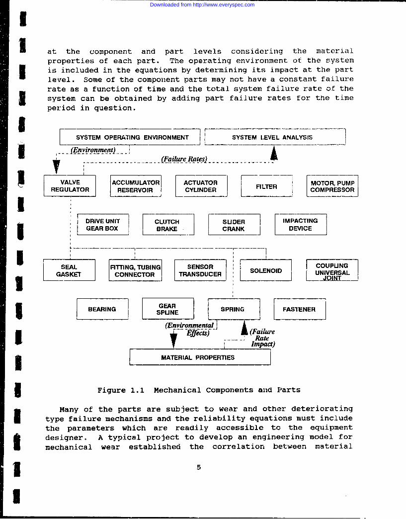
As part of the effort to develop a new methodology forpredicting the reliability of mechanical components, Figure 1.1illustrates the method of considering the effects of theenvironment and the operating stresses at the lowest indenturelevel. A component such as a valve assembly may consist of seals,springs, fittings, and the valve housing. The design life of theentire mechanical system is accomplished by evaluating the design

4


I

' at the component and part levels considering the materialproperties of each part. The operating environment ot the systemis included in the equations by determining its impact at the partlevel. Some of the component parts may not have a constant failurerate as a function of time and the total system failure rate of thesystem can be obtained by adding part failure rates for the timeperiod in question.

I SYSTEM OPERATING ENVIRONMENT- SYSTEM LEVEL ANALYSIS ]--- ...... (Xnv.i~ronnt~ent) .....

I AC(FMU L ureOR ats)

VALVE ACCUMULATOR ACTUATOR FILTERMOTOR, PUMPREGULATOR RESERVOIR - CYUNDER RLTER COMPRESSOR

DRIVE UNIT CLUTCH 1 SUDER 1 IMPACTINGGEAR BOX BRAKE CRANK DEVICE

SEAL FITTING, TUBING SENSOR SOEODCUPUNGGSKýET CONNECTOR TRANSDUCER SOENI UNIVERSALJ

S~~GEAR SRN AIEEBEARING SE SPRIN 7

Effects) *(Failure_____ __Rate

- ........ Impact)

1 MATERIAL PROPERTIES

3 IFigure 1.1 Mechanical Components and Parts

Many of the parts are subject to wear and other deterioratingtype failure mechanisms and the reliability equations must includethe parameters which are readily accessible to the equipmentdesigner. A typical project to develop an engineering model formechanical wear established the correlation between material

I


strength and surf ace wear. This method of predicting wearconsiders the materials involved, the lubrication properties, thestress imposed on the part and other aspects of the wear process.The relationship between the material properties and the wear ratewas used to establish generalized wear life equations for actuatorassemblies and other components subject to surface wear.

In another research project, lubricated and unlubricated splinecouplings were operated under controlled angular misalignment andloading conditions to provide empirical data to verify splinecoupling life prediction models. A special rotating mechanicalcoupling test machine was developed for use in generatingreliability data under controlled operating conditions. This high-speed closed loop testbed was used to establish the relationshipsbetween the type and volume of lubricating grease employed in thespline coupling and gear life. Additional tests determined theeffects of material hardness, torque, rotational speed and angularmisalignment on gear life.

Results of these wear research projects are being used todevelop and refine the reliability equations for those componentssubject to wear.

1.3 EXAMPLE DESIGN EVALUATION PROCEDUREA hydraulic valve assembly will be used to illustrate the

Handbook approach to predicting the reliability of mechanicalequipment. Developing reliability equations for all the differenttypes of hydraulic valves would be an impossible task since thereare over cre hundred different types of valve assemblies available.For example, some valves are named for the function they perform,e.g. check valve, regulator valve and unloader valve. Others arenamed for a distinguishing design feature, e.g. globe valve, needlevalve, solenoid valve. From a reliability standpoint, droppingdown one indenture level provides two basic types of valveassemblies: the poppet valve and the sliding action valve.

The example assembly chosen for analysis is a poppet valvewhich consists of a poppet assembly, spring, seals, and housing.

1.3.1 Poppet AssemblyThe functions of the poppet valve would indicate the primary

failure mode as incomplete closure of the valve resulting inleakage around the poppet seat. This failure mode can be caused bycontaminants being wedged between the poppet and seat, wear of thepoppet seat, and corrosion of the poppet/seat combination.External seal leakage, sticking valve stem, and damaged poppet

6


I! return spring are other failure modes which must be considered inthe design life of the valve.

A new poppet assembly may be expected to have a sufficientlysmooth surface for the valve to meet internal leakagespecifications. However, after some period of time contaminants5- will cause wear of the poppet assembly until leakage rate is beyondtolerance. This leakage rate, at which point the valve isconsidered to have failed, will depend on the application and toI what extent leakage can be tolerated.

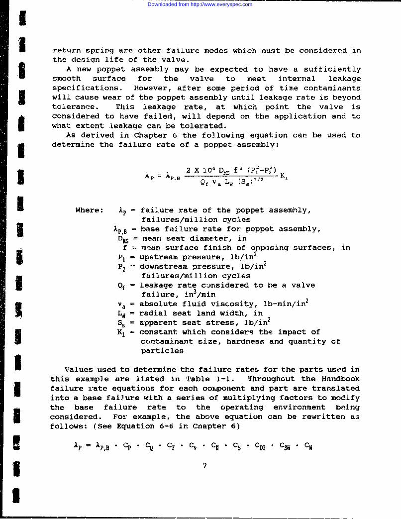
As derived in Chapter 6 the following equation car be used to5 idetermine the failure rate of a poppet assembly:

1P = 1P B 2 X 104 Dm f3 ,12 I KQ f va Lw (S.)' 1 2

I Where: 'X= failure rate of the poppet assembly,failures/million cycles

XP,B =base failure rate for poppet assembly,D•= mean seat diameter, in

f me-an surface finish of opposing surfaces, inP1 = upstream pressure, lb/in 2

P2 = downstream pressure, lb/infailures/million cycles

Qf = leakage rate cinsidered to be a valvefailure, in3/min

= = absolute fluid viscosity, Ib-min/in2

L = radial seat land width, inSS = apparent seat stress, lb/in2

K1 = constant which considers the impact ofcontaminant size, hardness and quantity ofparticles

Values used to determine the failure rates for the parts used inthis example are listed in Table 1-1. Throughout the Handbookfailure rate equations for each component and part are translatedinto a base failure with a series of multiplying factors to modifythe base failure rate to the operating environment beingI considered. For example, the above equatiun can be rewritten asfollows: (See Equation 6-6 in Cnapter 6)

SAP = AP,B - Cp . CQ - CF•* Cy - CS C Cc • C . CW

17


Where: Cp = Multiply~ing factor which considers the effectof fluid pressure on the base failure rate

CQ =Multiplyinq factor which considers the effectof allowable leakage on the base failure rate

CF = Multiplying factor which considers the effectof surface finish on the base failure rate

CV = Multiplying factor which considers the effectof fluid viscosity on the base failure rate

CN = Multiplying factor which considers the effectof contaminants on the base failure rate

Cs = Multiplying factor which considers the effectof seat stress on the base failure rate

C• = Multiplying factor which considers the effectof seat diameter on the base failure rate

CW = Multiplying factor which considers the effectof seat land width on the base failure rate

S = Multiplying factor which considers the effectof fluid flow rate on the base failure rate

The parameters in the failure rate equation can be located on anengineering drawing, by knowledge of design standards or by actualmeasurement. Other design parameters which have a minor effect onreliability are included in the base failure rate as determinedfrom field performance data.

1.3.2 Spring AssemblyDepending on the application, a spring may be in a static,

cyclic, or dynamic operating mode. In the current example of avalve assembly, the spring will be in a cyclic mode. The operatinglife of a mechanical spring arrangement is dependent upon thesusceptibility of the materials to corrosion and stress levels(static, cyclic or dynamic). The most common failure modes forsprings include fracture due to fatigue and excessive loss of lo&ddue to stress relaxation, Other failure mechanisms and causes maybe identified for a specific application. Typical failure rateconsiderations include: level of loading, operating temperature,cycling rate and corrosiveness of the fluid environment.

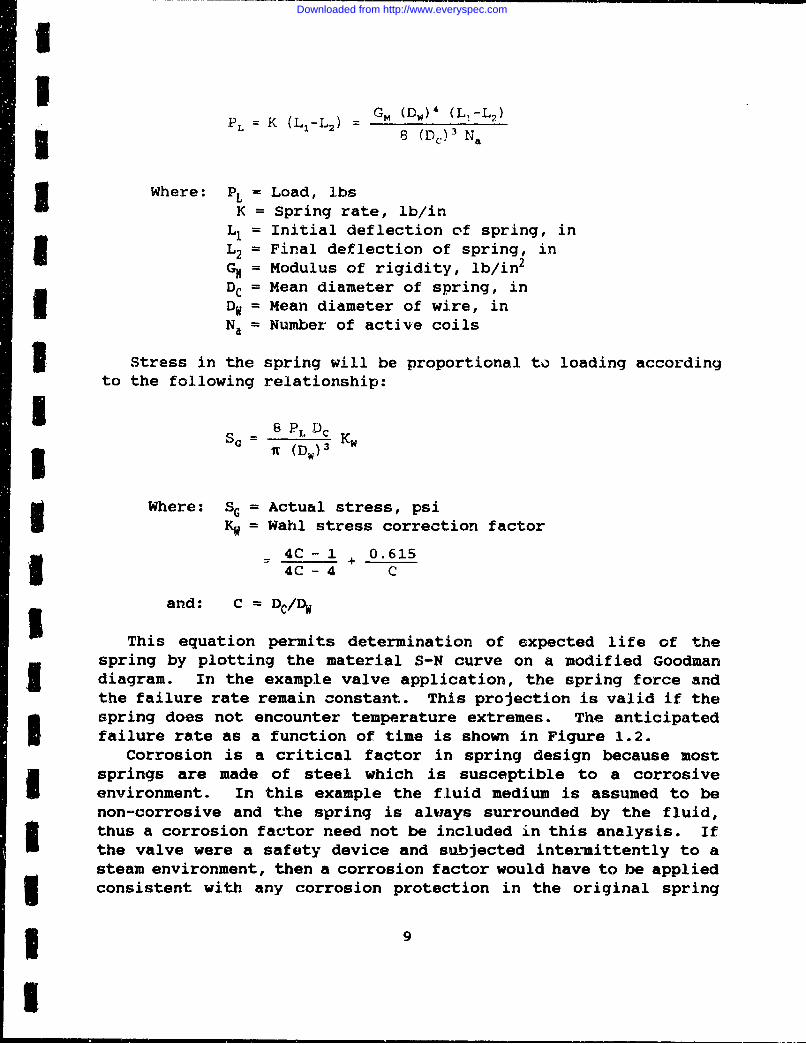
The failure rate of a spring depends upon the stress on thespring and the relaxation properties of the material. The load onthe spring is equal to the spring rate multiplied by the change inload per unit deflection and calculated as explained in Chapter 4.

8


U

P L = K ( ) Gm (Dw)4 (LI-L 2,)' 2 8 (D ) N &

Where: PL= Load, JbsI K = Spring rate, lb/inL= Initial deflection of spring, inL2 Final deflection of spring, inG_• Modulus of rigidity, lb/in2

DC = Mean diameter of spring, inDW = Mean diameter of wire, inNa = Number of active coils

3 Stress in the spring will be proportional to loading accordingto the following relationship:

I 8 PL Dcn (D W)3

Where: SG= Actual stress, psiKW = Wahl stress correction factor

i4C - 1 + 0.615S4C - 4 C

and: C Dc/DW

This equation permits determination of expected life of thespring by plotting the material S-N curve on a modified Goodmandiagram. In the example valve application, the spring force andthe failure rate remain constant. This projection is valid if thespring does not encounter temperature extremes. The anticipated

•I failure rate as a function of time is shown in Figure 1.2.Corrosion is a critical factor in spring design because most

springs are made of steel which is susceptible to a corrosiveI environment. In this example the fluid medium is assumed to benon-corrosive and the spring is always surrounded by the fluid,thus a corrosion factor need not be included in this analysis. If

1 the valve were a safety device and subjected intermittently to asteam environment, then a corrosion factor would have to be applied

* 1consistent with any corrosion protection in the original spring

*9

I


design.

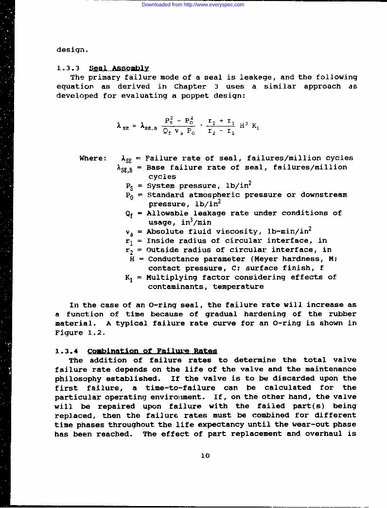
1.3.3 Beal- alyThe primary failure mode of a seal is leakage, and the following

equation as derived in Chapter 3 uses a similar approach asdeveloped for evaluating a poppet design:

~2 2 'PS PO - r 2 + r1 3Kl sz sB'BQt V a PO 12 - 11H3K

Where: ISE = Failure rate of seal, failures/million cyclesXSE,B = Base failure rate of seal, failures/million

cyclesPS = System pressure, lb/in2

P0 = Standard atmospheric pressure or downstreampressure, lb/in2

Qf = Allowable leakage rate under conditions ofusage, in 3 /min

Va= Absolute fluid viscosity, lb-min/in2

r= Inside radius of circular interface, inr 2 = Outside radius of circular interface, in

H = Conductance parameter (Meyer hardness, M;contact pressure, C; surface finish, f

K= Multiplying factor considering effects ofcontaminants, temperature

In the case of an 0-ring seal, the failure rate will increase asa function of time because of gradual hardening of the rubbermaterial. A typical failure rate curve for an 0-ring is shown inFigure 1.2.

1.3.4 Combination of Failu-e RatesThe addition of failure rates to determine the total valve

failure rate depends on the life of the valve and the maintenancephilosophy established. If the valve is to be discarded upon thefirst failure, a time-to-failure can be calculated for theparticular operating environment. If, on the other hand, the valvewill be repaired upon failure with the failed part(s) beingreplaced, then the failure rates must be combined for differenttime phases throughout the life expectancy until the wear-out phasehas been reached. The effect of part replacement and overhaul is

10


I

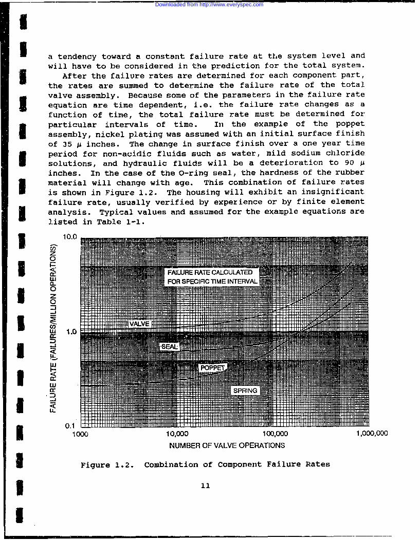
UI a tendency toward a constant failure rate at the system level andwill have to be considered in the prediction for the total system.3 After the failure rates are determined for each component part,the rates are summed to determine the failure rate of the totalvalve assembly. Because some of the parameters in the failure rateequation are time dependent, i.e. the failure rate changes as a

function of time, the total failure rate must be determined forI particular intervals of time. In the example of the poppet

assembly, nickel plating was assumed with an initial surface finishof 35 A inches. The change in surface finish over a one year time

I period for non-acidic fluids such as water, mild sodium chloridesolutions, and hydraulic fluids will be a deterioration to 90 pinches. In the case of the 0-ring seal, the hardness of the rubberU material will change with age. This combination of failure ratesis shown in Figure 1.2. The housing will exhibit an insignificantfailure rate, usually verified by experience or by finite element

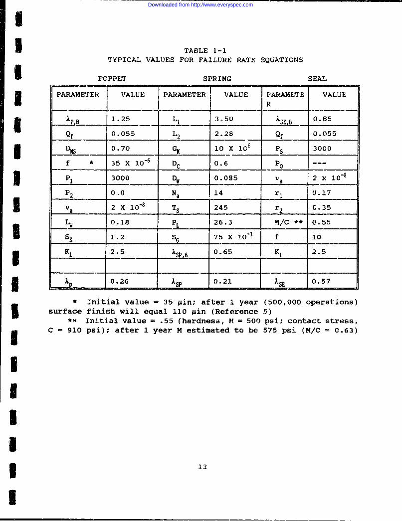
SI analysis. Typical values and assumed for the example equations arelisted in Table 1-1.

I 10.0

z

0 SFAWR RAT CALCULATED

W FOR SPECIFIC 11ME INTE•

w

I 0

077-3

-SEAT

IW

0.1I1000 10,000 100,000 1,000,000NUMBER OF VALVE OPERATIONS

I Figure 1.2. Combination of Component Failure Rates

3 1


1.4 VALIDATION OF RELIABILITY PREDICTION EQUATIONSA very limited budget for this project has prevented the

procurement, of a large number of components to perform thenecessary failure rate tests for all of the possible combinationsof loading roughness, operational environments, and designparameters to validate the equations. For example, valveassemblies were procured and tested at the Belvoir Research,Development and Engineering Center in Ft. Belvoir, Virginia. Thenumnber of failures for each test were predicted using the equationspresented in this Handbook. Failure rate tests were performed forseveral combinations of stress levels and results compared topredictions. Typical results are shown in Table 1-2.

The procedures presented in this Handbook should not beconsidered as the only methods for a design analysis. An engineerneeds many evaluation tools in his toolbox and new methods ofperforming dynamic modeling, finite element analysis and otherstress/strength evaluation methods must be used in combination toarrive at the best possible reliability prediction for mechanicalequipment.

The examples included in this introduction are intended toillustrate the point that there are no simplistic approaches topredicting the reliability of mechanical equipment. Accuratepredictions of reliability are best achieved by considering theeffects of the operating environment of the system at the partlevel. The failure rates derived from equations as tailored to theindividual application then permits an estimation of design lifefor any mechanical system.

It will be noted upon review of the equations that some of theparameters are very critical in terms of life expectancy. Forexample, the failure rate equation for the poppet assembly containsthe surface finish parameter which deteriorates as a function oftime and is raised to the third power. The same problem exists inmany of the equations for predicting the reliability of mechanicalequipment. Additional research is needed to obtain additionalinformation on some of these cause and effect relationships for usein the equations and continual improvement to the Handbook.

12


I

- TABLE 1-1"TYPICAL VALUES FOR FAILURE RATE EQUATIONS

POPPET SPRING SEAL

PARAMETER VALUE PARAMETER VALUE PARAMETE VALUE

Ape 1.25 Li 3.50 __E, 0.85__

Qf 0.055 L2 2.28 Qf 0.055

3 D__ 0.70 GK 10 X 1C6 PS 3000

f * 35 X 10 6 DC 0.6 PO...

3 P1 3000 DW 0.085 Va 2 x 10-8

P2 0.0 Na 14 rI 0.17

Va 2 X 10-8 TS 245 r2 C.35

LW 0.18 PL 26.3 M/C ** 0.55

SS 1.2 SG 75 X 10-3 f 10

KI 2.5 0.65 K1 2.5

A 0.26 ASP 0.21 ASE 0.57

Initial value = 35 uin; after 1 year (500,000 operations)5 surface finish will equal 110 min (Reference 5)*• Initial value = .55 (hardness, It = 500 psi; contact stress,

C = 910 psi); after 1 year M estimated to be 575 psi (M/C = 0.63)

* 13

i


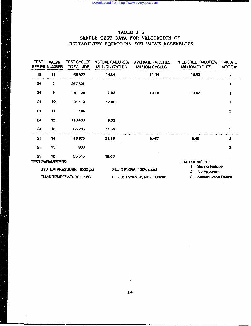
TABLE 1-2SAMPLE TEST DATA FOR VALIDATION OF

RELIABILITY EQUATIONS FOR VALVE ASSEMBLIES

TEST VALVE TEST CYCLES ACTUAL, FAILURES/ AVERAGE FAILURES/ PREDICTED FAILURES/ FAILURESERIES NUMBER TO FAILURE MIWON CYCLES MILLWON CYCLES MILLON CYCLES MODE #

15 11 68,322 14.64 14.64 18.02 3S.................... ...... ............................................................................................................................ ....................

24 8 257,827 1

24 9 131,126 7.63 10.15 10.82 1

24 10 81,113 12.33 1

24 11 104 2

24 12 110,488 9.05 1

24 13 86,285 11.59 1

25 14 46,879 21.33 19.67 8.45 2

25 15 300 3

25 18 55,545 18.00 1TEST PARAMETERS: FAILURE MODE:

1 - Spring FatigueSYSTEM PRESSURE: 3500 psi FLUID FLOW: 100% reded 2 - no F

2 - No Apparent

FLUID TEMPERATURE: 90"C FLUID: Hydraulic, MIL-H-83282 3 - Accumulated Debris

14


£

CHAPTER 2

DEFINITIONS

This report is intended for use by reliability analysts andequipment designers. Accordingly, a review of some basic terms willhelp to establish a cross reference for these twodisciplines. MIL-STD-721 should be referred ý:o for basic

SI reliability definitions.

• Base Failure Rate - A failure rate for a component or part infailures per million hours or failures per million operationsI depending on the application and derived from a data base where theexact design, operational, and environmental parameters are known.I• Multiplying facto~rs are then used to adjust the base failure rateto the new operating environment.

• Brake Lining - a frictional material used for stopping orretarding the relative movement of two surfaces.

0 Coefficient of Friction - this relationship is the ratiobetween two measured forces. The denominator is the normal forcepressing two surfaces together. The numerator is the frictionalforce resisting the motion of one surface over other.

* Contamination - foreign matter or particles in a fluid systemthat are transported during its operation and which may bedetrimental to system performance or even cause failure of a

component.0 Corrosion - the slow destruction of materials by chemical

agents and/or electromechanical reactions.* Creep - continuous increase in deformation under constant or

decreasing stress.0 Dependent failure - failure caused by failure of an associated

item or by a common agent.I Dirt lock - complete impedance of movement caused by straycontaminant particles wedged between moving parts.

* Endurance Limit - the stress level value when plotted as afunction of the number of stress cycles at which point a constantstress value is reached.1 * External leakage - leakage resulting in loss of fluid to theexternal environment.

Failure mode - the indicator or symptom by which a failure isI evidenced.

15


. Failure rate - the probable number of times that a givencomponent will fail during a given period of operation underspecified operating conditions. Failure rate may be in terms oftime, cycles, revolutions, miles, etc.

. Fatigue - the cracking, fracture or breakage of mechanicalmaterial due to the application of repeated, fluctuating orreversed mechanical stress less than the tensile strength of thematerial.

- Friction Material - a product manufactured to resist slidingcontact between itself and another surface in a controlled manner.

* Hardness - a measure of material resistance to permanent orplastic deformation equal to a given load divided by the resultingarea of indentation.

* Independent failure - a failure of a device which is notcaused by or related to failure of another device.

* Internal leakage - leakage resulting in loss of fluid in thedirection of fluid flow past the valving unit.

* Leakage - the flow of fluid through the interconnecting voidsformed when the surfaces of two materials are brought into contact.

• Mean cycles between failure - the total number of functioningcycles of a population of parts divided by the total number offailures within the population during the same period of time. Thisdefinition is appropriate for the number of hours as well as forcycles.

* Mean cycles to failure - the total number of functioningcycles divided by the total number of failures during the period oftime. This definition is appropriate for the number of hours aswell as for cycles.

* Modulus of Elasticity - Slope of the initial linear portion ofthe stress-strain diagram; the larger the value, the larger thestress required to produce a given strain. Also known as Young'sModulus.

0 Modulus of Rigidity - the rate of change of unit shear stresswith respect to unit shear stroin for the condition of pure shearwithin the proportional limit. Also called Shear Modulus ofElasticity.

, Poisson's Ratio - Ratio of lateral strain to axial strain ofa material when subjected to uniaxial loading.

o Random failures - failures that occur before wear out, are notpredictable as to the exact time -,f similar and are not associatedwith any pattern of similar failures. However, the number of randomfailures for a given population over a period of time at a constantfailure rate can be predicted.

16


I • Silting - an accumulation and settling of particles duringcomponent inrctivity.

Stiction - a change in performance characteiistics or completeimpedance of poppet or spool movement caused by wedging of minuteparticles between a poppet stem and housing or between spool andsleeve

. Stress - A measure of intensity of force acting on a definiteplane passing through a given point, measured in force per unit

* area.• Tensile Strength - Value of nominal stress obtained when the

maximum (or ultimate) load that the specimen supports is divided bythe cross-sectional area of the specimen. See Ultimate Strength

. Ultimate Strength - the maximum stress the material willSI withstand. See Tensile Strength

I Viscosity - a measure of internal resistance of a fluid whichtends to prevent it from flowing.

• Wear out failure - a failure which occurs as a result ofmechanical, chemical or electrical degradation.

• Yield strength - The stress that will produce a small amountof permansnt deformation, generally a strain equal to 0.1 or 0.2percent of the length of the specimen.

III

I

3 17

I


I

II

1I


I

18I

JI


CHAPTER 3

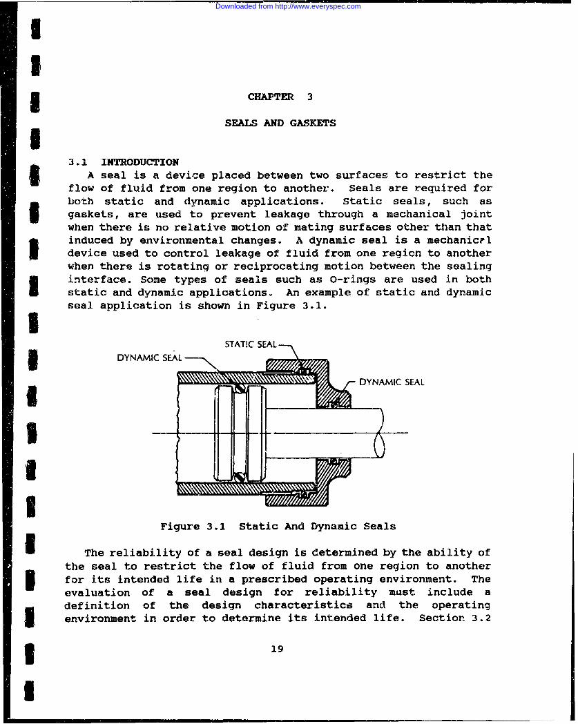
SEALS AND GASKETSI3.1 INTRODUCTION£ A seal is a device placed between two surfaces to restrict theflow of fluid from one region to another. Seals are required forboth static and dynamic applications. Static seals, such asgaskets, are used to prevent leakage through a mechanical jointwhen there is no relative motion of mating surfaces other than that

I induced by environmental changes. A dynamic seal is a mechanicrldevice used to control. leakage of fluid from one region to anotherwhen there is rotating or reciprocating motion between the sealing

I • interface. Some types of seals such as O-rings are used in bothstatic and dynamic applications. An example of static and dynamicseal application is shown in Figure 3.1.I

ISTATIC SEAL

IDYNAMIC SEAL

I

Figure 3.1 Static And Dynamic Seals

I The reliability of a seal design is determined by the ability ofthe seal to restrict the flow of fluid from one region to anotherfor its intended life in a prescribed operating environment. Theevaluation of a seal design for reliability must include adefinition of the design characteristics and the operatingenvironment in order to determine its intended life. Section 3.2

319


discusses the reliability of gaskets and static seals. Adiscussion of dynamic seal reliability is contained in Section 3.3.

3.2 GASKETS AND STATIC SEALS

3. 2. 1 r.Id/re Moder

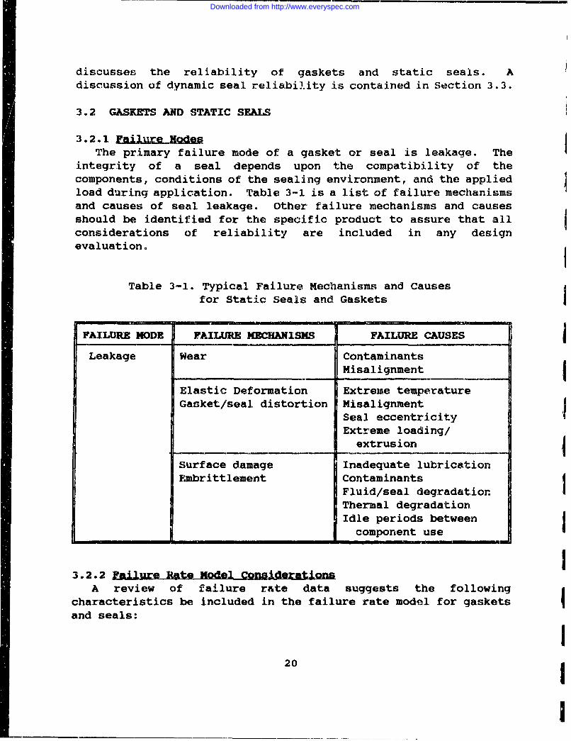
The primary failure mode of a gasket or seal is leakage. Theintegrity of a seal depends upon the compatibility of thecomponents, conditions of the sealing environment, and the appliedload during application. Table 3-1 is a list of failure mechanismsand causes of seal leakage. Other failure mechanisms and causesshould be. identified for the specific product to assure that allconsiderations of reliability are included in any designevaluation.

Table 3-1. Typical Failure Mechanisms and Causesfor Static Seals and Gaskets

FAILURE MODE FAILURE MECHANISMS FAILURE CAUSES JLeakage Wear Contaminants

Misalignment IElastic Deformation Extreme temperatureGasket/seal distortion Misalignment

Seal eccentricityExtreme loading/

extrusion ISurface damage Inadequate lubricationEmbrittlement Contaminants

Fluid/seal degradationThermal degradationIdle periods between

component use

3.2.2 Failure Rate Model ConsiderationsA review of failure r&te data suggests the following

characteristics be included in the failure rate model for gaskets !and seals:

20


I * Static vs. dynamic conditionsM Material characteristics

• Amount of seal compression• Surface irregularities• Seal size

Extent of pressure pulses• Contamination level• Fluid/material compatibilityB Leakage requirements• Fluid viscosity• Q. C./ Manufacturing process• Fluid pressure

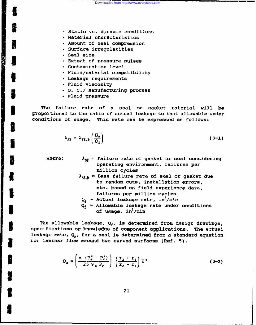
The failure rate of a seal or gasket material will beI proportional to the ratio of actual leakage to that allowable underconditions of usage. This rate can be expressed as follows:

5S A6SH, (3-1)

Where: ASE Failure rate of gasket or seal consideringI operating environment, failures parmillion cycles

SEB = Base failure rate of seal or gasket dueto random cuts, installation errors,etc. based on field experience data,3 failures per million cycles

Qa - Actual leakage rate, in 3/minQf - Allowable leakage rate under conditions

of usage, in 3/min

The allowable leakage, Qf, is determined from desigr drawings,specifications or knowledge of component applications. The actualleakage rate, Qa, for a seal is determined from d standard equation3 for laminar flow around two curved surfaces (Ref. 5).

i(P,-P r+r. . 3 (3-2)Ql25va PC, 1 2 Z- X

3 21


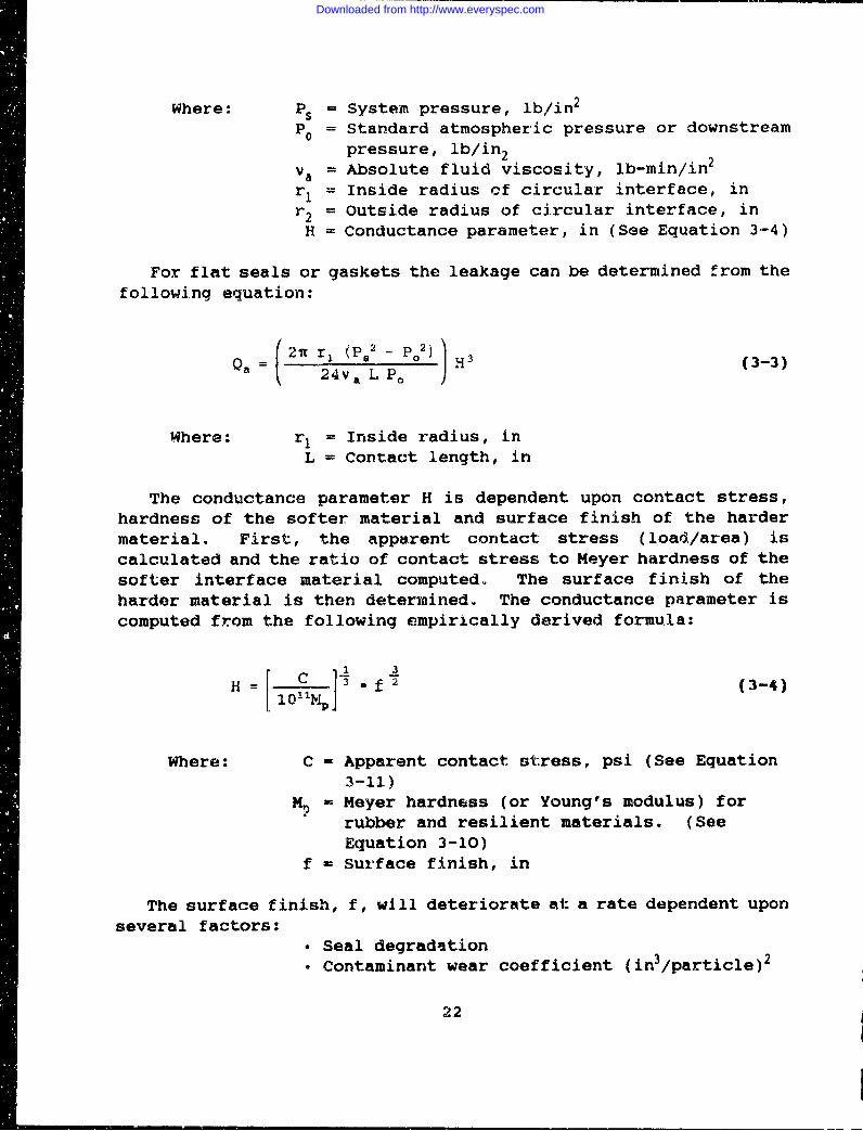
Where: Ps = System pressure, lb/in2

P0 = Standard atmospheric pressure or downstreampressure, lb/in2

Va = Absolute fluid viscosity, lb-min/in2

r, = Inside radius of circular interface, inr2 = Outside radius of circular interface, in

H = Conductance parameter, in (See Equation 3-4)

For flat seals or gaskets the leakage can be determined from thefollowing equation:

(_27T r (P, 2 - P 2) H 3 (3-3)1a 24va L PO

Where: r, = Inside radius, inL = Contact length, in

The conductance parameter H is dependent upon contact stress,hardness of the softer material and surface finish of the hardermaterial. First, the apparent contact stress (load/area) iscalculated and the ratio of contact stress to Meyer hardness of thesofter interface material computed. The surface finish of theharder material is then determined. The conductance parameter iscomputed from the following empirically derived formula:

rl 0MP 3 " f 2 (3-4)

Where: C = Apparent contact stress, psi (See Equation3-11)

M2 = Meyer hardness (or Young's modulus) forrubber and resilient materials. (SeeEquation 3-10)

f = Surface finish, in

The surface finish, f, will deteriorate at a rate dependent uponseveral factors:

"* Seal degradation"• Contaminant wear coefficient (in 3/particle) 2

22


I

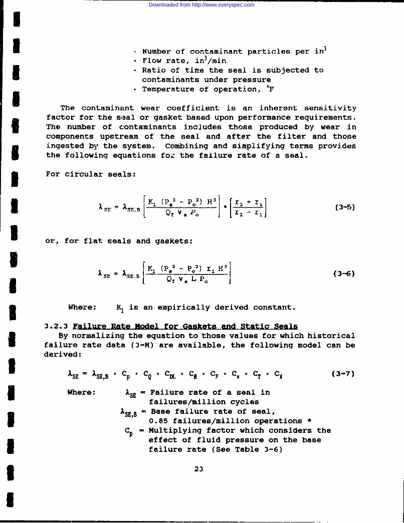
I Number of contaminant particles per in 3

• Flow rate, in 3/min• Ratio of time the seal is subjected to

contaminants under pressure• Temperature of operation, OF

The contaminint wear coefficient is an inherent sensitivityfactor for the seal or gasket based upon performance requirements.The number of contaminants includes those produced by wear incomponents upstream of the seal and after the filter and thoseingested by the system. Combining and simplifying terms providesthe following equations foz the failure rate of a seal.

For circular seals:

x SE ' ISEB K, (P2 - P 02 ) H 3 Fr 2 + r1i

QfVa'P : 11 (5

or, for flat seals and gaskets:

ISE ': ISE.B [K1 (PI, a2 )P zrl H j(3-6)I3 Where: KI is an empirically derived constant.

3.2.3 Failure Rate Model for Gaskets and Static SealsBy normalizing the equation to those values for which historical

failure rate data (3-M) are available, the following model can bederived:

E SE - SE,B Cp•CQ DLC•C CF•C,•CT•CJ, (3-7)

SWhere: ASE = Failure rate of a seal infailures/million cycles

ASEB = Base failure rate of seal,I 0.85 failures/million operations *C = Multiplying factor which considers the

effect of fluid pressure on the basefailure rate (See Table 3-6)

3 23

I


-Ci

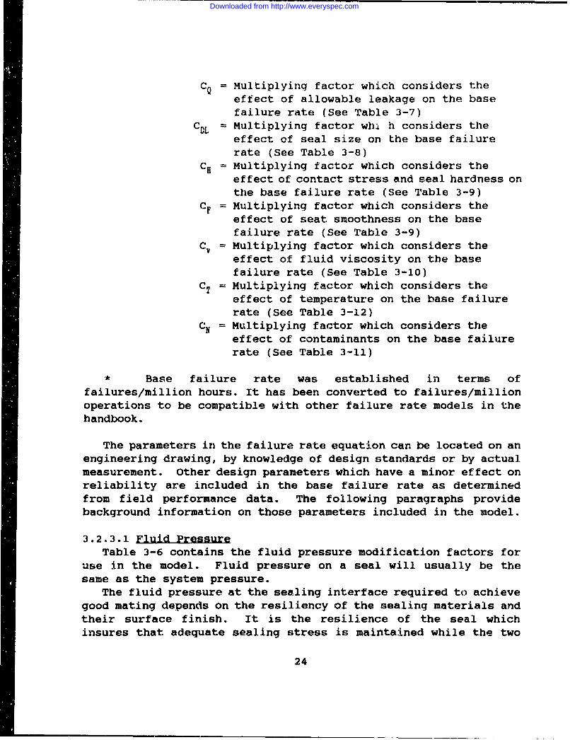
CQ = Multiplying factor which considers theeffect of allowable leakage on the basefailure rate (See Table 3-7)

CDL = Multiplying factor wha h considers theeffect of seal size on the base failurerate (See Table 3-8)

CH = Multiplying factor which considers theeffect of contact stress and seal hardness onthe base failure rate (See Table 3-9)

CF = Multiplying factor which considers theeffect of seat smoothness on the basefailure rate (See Table 3-9)

CV = Multiplying factor which considers theeffect of fluid viscosity on the basefailure rate (See Table 3-10)

CT = Multiplying factor which considers theeffect of temperature on the base failurerate (See Table 3-12)

CN = Multiplying factor which considers theeffect of contaminants on the base failurerate (See Table 3-11)

* Base failure rate was established in terms offailures/million hours. It has been converted to failures/millionoperations to be compatible with other failure rate models in thehandbook.

The parameters in the failure rate equation can be located on anengineering drawing, by knowledge of design standards or by actualmeasurement. Other design parameters which have a minor effect onreliability are included in the base failure rate as determinedfrom field performance data. The following paragraphs providebackground information on those parameters included in the model.

3.2.3.1 Fluid PressureTable 3-6 contains the fluid pressure modification factors for

use in the model. Fluid pressure on a seal will usually be thesame as the system pressure.

The fluid pressure at the sealing interface required to achievegood mating depends on the resiliency of the sealing materials andtheir surface finish. It is the resilience of the seal whichinsures that adequate sealing stress is maintained while the two

24


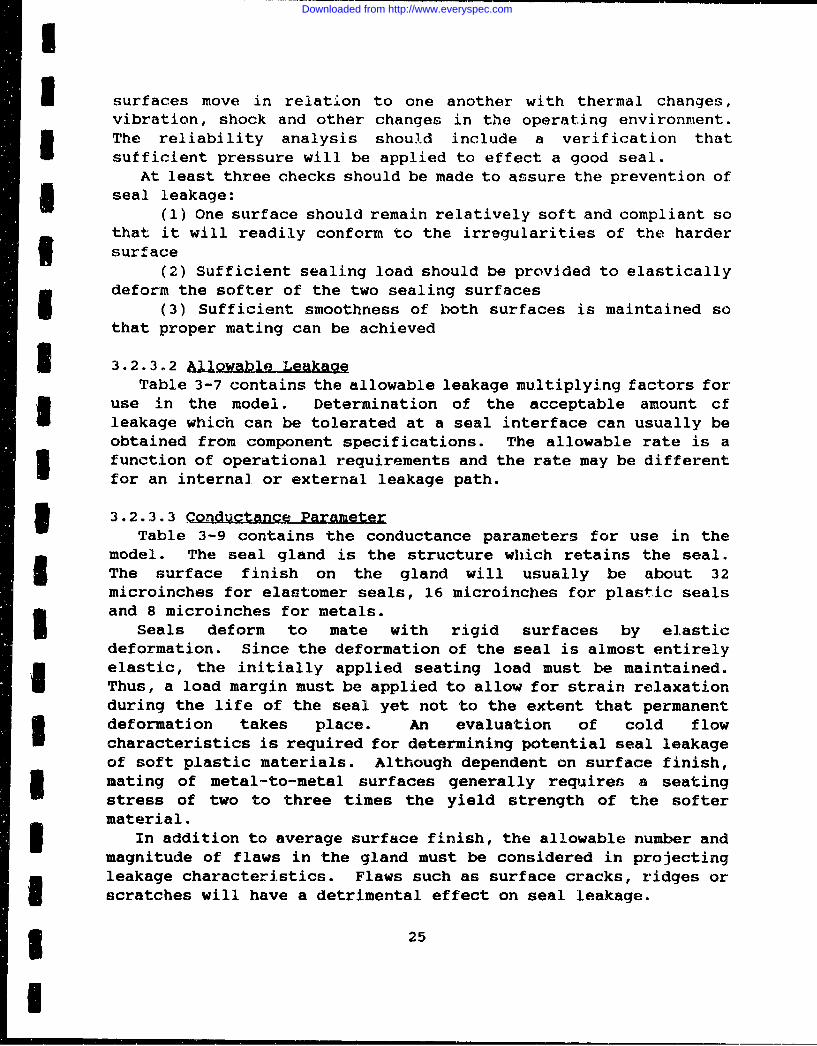
UI surfaces move in relation to one another with thermal changes,vibration, shock and other changes in the operating environment.The reliability analysis should include a verification thatsufficient pressure will be applied to effect a good seal.

At least three checks should be made to assure the prevention of* seal leakage:

(1) One surface should remain relatively soft and compliant sothat it will readily conform to the irregularities of the harder

Si surface(2) Sufficient sealing load should be provided to elastically

deform the softer of the two sealing surfacesI (3) Sufficient smoothness of both surfaces is maintained sothat proper mating can be achieved

3 3.2.3.2 A&.yL]•wb LeakageTable 3-7 contains the allowable leakage multiplying factors for

use in the model. Determination of the acceptable amount cfleakage which can be tolerated at a seal interface can usually beobtained from component specifications. The allowable rate is afunction of operational requirements and the rate may be differentfor an internal or external leakage path.

3 J3.2.3.3 Conductance ParameterTable 3-9 contains the conductance parameters for use in the

model. The seal gland is the structure which retains the seal.The surface finish on the gland will usually be about 32microinches for elastomer seals, 16 microinches for plastic sealsS and 8 microinches for metals.

Seals deform to mate with rigid surfaces by elasticdeformation. Since the deformation of the seal is almost entirelyelastic, the initially applied seating load must be maintained.Thus, a load margin must be applied to allow for strain relaxationduring the life of the seal yet not to the extent that permanentdeformation takes place. An evaluation of cold flowcharacteristics is required for determining potential seal leakageof soft plastic materials. Although dependent on surface finish,mating of metal-to-metal surfaces generally requires a seatingstress of two to three times the yield strength of the softermaterial.

In addition to average surface finish, the allowable number andmagnitude of flaws in the gland must be considered in projectingleakage characteristics. Flaws such as surface cracks, ridges orscratches will have a detrimental effect on seal leakage.

3 I25

I|


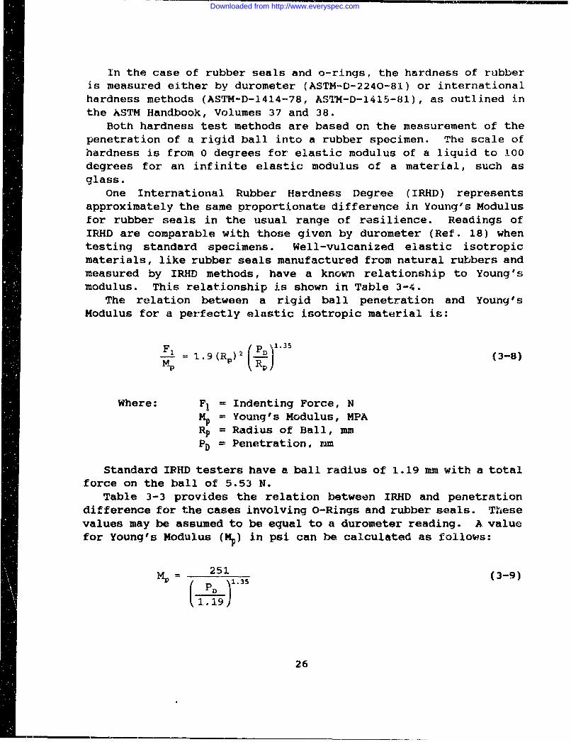
In the case of rubber seals and o-rings, the hardness of rubberis measured either by durometer (ASTM-D-2240-81) or internationalhardness methods (ASTM-D-1414-78, ASTM-D-1415-81), as outlined inthe ASTM Handbook, Volumes 37 and 38.

Both hardness test methods are based on the measurement of thepenetration of a rigid ball into a rubber specimen. The scale ofhardness is from 0 degrees for elastic modulus of a liquid to 100degrees for an infinite elastic modulus of a material, such asglass.

One International Rubber Hardness Degree (IRHD) representsapproximately the same proportionate difference in Young's Modulusfor rubber seals in the usual range of resilience. Readings ofIRHD are comparable with those given by durometer (Ref. 18) whentesting standard specimens. Well-vulcanized elastic isotropicmaterials, like rubber seals manufactured from natural rubbers andmeasured by IRHD methods, have a known relationship to Young'smodulus. This relationship is shown in Table 3-4.

The relation between a rigid ball penetration and Young'sModulus for a perfectly elastic isotropic material is:

F1 = 1.9 (R))2 (3-8)

Where: F1 = Indenting Force, NS= Young's Modulus, MPARP = Radius of Ball, mm

PD= Penetration, mm

Standard IPHD testers have a ball radius of 1.19 mm with a totalforce on the ball of 5.53 N.

Table 3-3 provides the relation between IRHD and penetrationdifference for the cases involving O-Rings and rubber seals. Thesevalues may be assumed to be equal to a durometer reading. A valuefor Young's Modulus (HP) in psi can be calculated as follows:

251 (3-9)MP (D )1.35

1.196

26


1

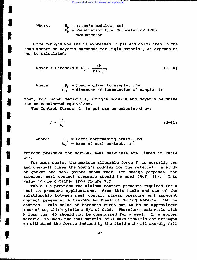
Where: Mý = Young's modulus, psi) D = Penetration from Durometer or 1RHD

3 measurement

Since Young's modulus is expressed in psi and calculated in thesame manner as Meyer's Hardness for Rigid Material, an expressioncan be calculated:

Meyer's Hardness = M -- D2 (3-10)-IWhere: PF = Load applied to sample, lbs

D11 = diameter of indentation of sample, in

Then, for rubber materials, Young's modulus and Meyer"s hardnessI can be considered equivalent.The Contact Stress, C, in psi can be calculated by:

C Fc (3-11)

Where: Fc = Force compressing seals, lbsIAsc = Area of seal contact, in 2

3 Contact pressure for various seal materials are listed in Table3-5.

For most seals, the maximum allowable force F. is normally twoand one-half times the Young's modulus for the material. A studyof gasket and seal joints shows that, for design purposes, theapparent seal contact pressure should be used (Ref. 38). This3 value can be obtained from Figure 3.2.

Table 3-5 provides the minimum contact pressure required for aseal in pressure applications. From this table and use of therelationship between seal contact stress pressure and apparentcontact pressure, a minimum hardness ef O-ring material -an bededuced. This value of hardness turns out to be an approximateIRHD of 60, which yields a X/C of 0.35. Therefore, materials withM less than 60 should not be, considered for a seal. If a softermaterial is used, the seal material will have insufficient strengthto withstand the forces induced by the fluid and ý;ill rap.,diy fail

327


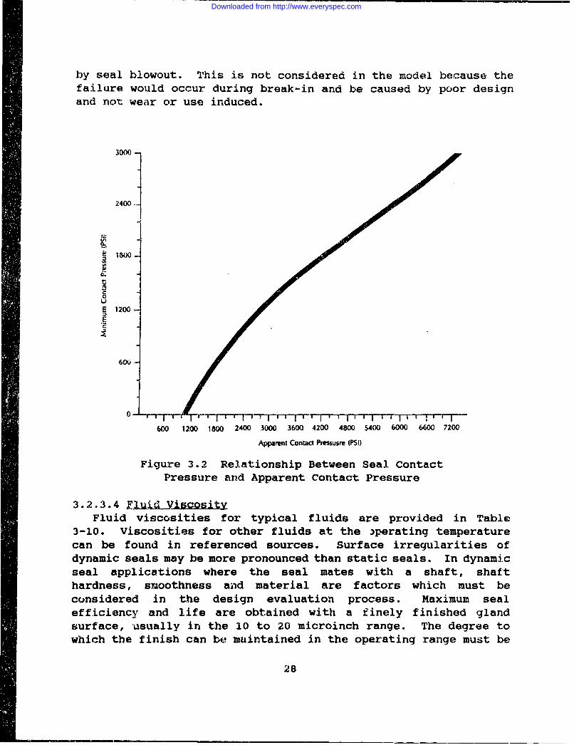
by seal blowout. This is not considered in the model because thefailure would occur during break-in and be caused by poor designand not wear or use induced.

3000

2400

S1800-

C0

E 1200

E

0 rr -- FT- r--7 r -T -7T -Tr-r I I' I I I I I'

600 1200 1800 2400 3000 3600 4200 4800 5400 6000 6600 7200

Apparnit Contact Prsusm (PSI)

Figure 3.2 Relationship Between Seal ContactPressure and Apparent Contact Pressure

3.2.3.4 fuiYLM sityFluid viscosities for typical fluids are provided in Table

3-10. Viscosities for other fluids at the 3perating temperaturecan be found in referenced sources. Surface irregularities ofdynamic seals may be more pronounced than static seals. In dynamicseal applications where the seal mates with a shaft, shafthardness, smoothness and material are factors which must beconsidered in the design evaluation process. Maximum sealefficiency and life are obtained with a finely finished glandsurface, usually in the 10 to 20 microinch range. The degree towhich the finish can be muintained in the operating range must be

28


I considered when determining the surface finish of the gland for usein the model.

33.2.3.5 F1uid ContaminantsThe quantities of contaminants likely to be generated by

upstream components are listed in Table 3-11. The number ofcontaminants depends upon the design, the enclosures surroundingthe seal, its physical placement within the system, maintenancepractices and quality control. The number of contaminants may haveto be estimated from experience with similar components.

3 3.2.3.6 0Derating TemperatureThe operating temperature has a definite effect on the aging

process of elastomer and rubber seals. Elevated temperatures,3 those temperatures above the normal use temperatures, tend tocontinue the vulcanization or curing process of the materials,

I thereby, significantly changing the original characteristics of theseal or gasket. It can cause increased hardening, brittleness,loss of resilience, cracking, and excessive wear. Since a changein these characteristics has a definite effect on the failure rateof the component, a reliability adjustment must be made.

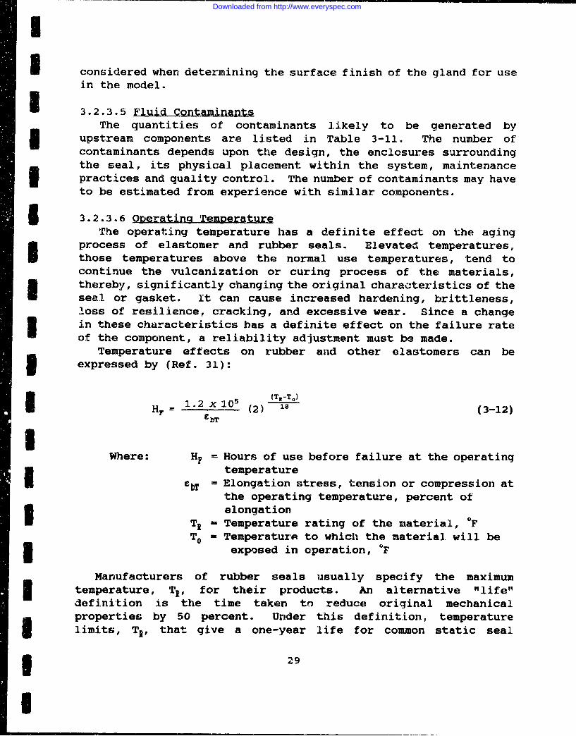
Temperature effects on rubber and other elastomers can be3 expressed by (Ref. 31):

.1.2 x 105 (T 3 -T°- )IH 1.2 (2) 'e (3-12)£bT-I

Where: HF = Hours of use before failure at the operatingtemperatureIbT = Elongation stress, tension or compression atthe operating temperature, percent ofelongation

TI - Temperature rating of the material, 0FTo M Temperature to which the material will be3 exposed in operation, 'F

Manufacturers of rubber seals usually specify the maximumStemperature, TI, for their products. An alternative "life"

definition is the time taken to reduce original mechanicalproperties by 50 percent. Under this definition, temperatureI limits, TR, that give a one-year life for common static seal

* 29


materials are given in Table 3-13.For O.-Rings, it is standard practice to design the seals for £bT

= 25 percent compression.

CT =-La (3-13)FR

Where: CT = Temperature factor.F0 = Failure rate of operating component in

failures per million cycles(See Equation 3-14).

FR - Failure rate of components, operating atrated temperature, measured in failuresper million cycles.

F 106 (3-14)HF NHC

Where: NB = Operating cycles per hr.

These expressions are only valid below the temperature at whichthe seal or gasket begins to melt or char. For the case where allparameters are equal except temperature;

CT 1 (3-15)

18

3.2.3.7 Qther ConsiderationsThose failure rate considerations not specifically included in

the model but rather included in the base failure rates are asfollows:

"" Proper selection of seal materials with appropriatecoefficients of thermal expansion for the applicable fluidtemperature and compatibility with fluid medium.

"• Potential corrosion from the gland, seal, fluid interface."* Possibility of the seal rolling in its groove when system

surges are encountered.

30


• If 0-rings can not be installed or replaced easily they aresubject to being cut by sharp gland edges.

E3.3 DYNAMIC SEALS

I 3.3.1 FAilure NodeThe mechanical seal may be used to seal many different liquids

at various speeds, pressures, and temperatures. The sealingsurfaces are perpendicular to the shaft with contact between theprimary and mating rings to achieve a dynamic seal.

The wear occurs between the primary ring and mating ring. ThisI surface contact is maintained by a spring. There is a film ofliquid maintained between the sealing surfaces to eliminate as muchfriction as possible. For most dynamic seals, the three commonI points of sealing contact occur between the following points:

1. Mating surfaces between primary and mating rings.2. Between the rotating component and shaft or sleeve.

- 3. Between the stationary component and the gland plate.The various failure mechanisms and causes for mechanical seals

S1 are listed in Table 3-2.

3.3.2 Failure Rate Model3The mating ring is usually a separate replaceable part. Thestatic seal and the mating ring are separated from leakage to theI igland plate by the O-Ring or static seal. Of greatest importancewith dynamic seals is a properly designed seal face. The matingsurfaces are usually made from different materials. The propermaterials must be matched so that excessive heat isn't generatedI from the dynamic motion of the seal faces. Too much heat can causethermal distortions on the face of the seal and cause gaps whichcan increase the leakage rate. It can also cause material changesthat can significantly increase the seal wear rate. Therefore,careful material selection should be included for each surface ofU Ithe dynamic seal face. Equation (3-17) (Ref. 26) expresses suchcoefficients of friction, and wear rates. Table 3-14 showsfrictional values for various seal face materials.

Qs - C1 " PV • p * a0 (3-17)

3 Where: Q8 = Heat input from the seal, BTU/n(W)C1 = Numerical constant; 0.077 for USCS units and

1.0 for SIPV - Pressure-velocity coefficient (See Eq. 3-18)

131


I.= Coefficient of friction (See Table 3-14) 1a0 Seal face area, in 2 (m22 )

Two important parameters that effect seal wear are seal facepressure and fluid velocity. These parameters multiplied togetherprovide a "PV" factor. The following equation defines the "PV"factor.

PV= [DP (bk) + ZE (3-18)L aoJ

Where: DP = Pressure differential across seal face,psi (N/mr2 )

b = Seal balance, the ratio of hydraulic closingarea to seal face area.

k = Pressure gradient factor, See Table 3-15FSp = Seal spring load. Lb (N)VX = Fluid velocity at the seal mean face

diameter, ft/min (m/s)

The frictional aspects of materials are not only important froma reliability viewpoint, but also from an efficiency aspect. Themore resistance a system incurs, the more power is lost and alsothe lower the efficiency value for the component. Therefore, theextra cost for a component with special wear resistant seals maywell pay for itself through savings in powering the component plusthe savings involved with lower maintenance costs. There should bespecial consideration for tradeoffs involved with each type of sealmaterial. For example, solid silicon carbide has excellentabrasion resistance, good corrosion resistance, and moderatethermal shock resistance. This material has better qualities thana carbon-graphite base material but has a PV value of 500,000lb/in-min while carbon-graphite has a 50,000 lb/in-min PV value.With all other values being the same, the heat generated would befive times greater for solid silicon carbide than forcarbon-graphite materials. The required cooling flow to the solid Isilicon carbide seal would be larger to maintain the film thicknesson the dynamic seal faces. If this cooling flow can't bemaintained, then an increase in wear would occur due to higher Isurface temperatures. The analyst should perform tradeoff analysisfor each candidate design to maximize reliability. I

32

- ' • n • • i P i • i" • 1 • I • •" In , z . • • .. : I


SI The PV factor will be incorporated into the seal reliabilitymodel. Most of the seal modifying factors will remain the same asU- the ones previously specified by Equation 3-7. The seal model ismodified as shown in Equation 3-19.

ISE SE,B CF Cv CTC C CPV CQ (3-19)

XSEB is the base failure rate and the multiplying factors areI equal to the ones previously defined in Equation (3-7) with theexception of C and CT. The temperature factor, CT, and thepressure/velocity factor, C1,, are presently discussed.

I C• is the multiplying factor that multiplies the base failurerate by the ratio of PV value for actual seal operation to designPV value. The values for PV, arnd PVop used in Equation (3-20) willuse the PV formulation in Equation (3-18).

I C= PV / PVD (3-20)

Where: PVo = PV factor for the original design3 PV• = PV factor for actual seal operation

The temperature factor, CT is formulated from research showingI that the values for PV will decrease by one-half when the operatingtemperature is doubled. Equation (3-21) represents this

I relationship-

CT = 1 + To - TR (3-21)| TR

Where: To = Operating temperatureTR = Rated temperature

3 An additional important seal design consideration is sealbalance. This performance characteristic measures how effectivethe seal mating surfaces match. The seal load at the dynamicfacing may be too high causing the liquid film to be squeezed outand vaporized - thus causing a high wear rate. The seal surfacesalso have structural load limitations that, if breached, may causepremature failures. The dynamic facing pressure can be controlledby manipulating the hydraulic closing area. The fluid pressurefrom one side of the primary ring causes a certain amount of force

133


to impinge on the dynamic seal face. This force can be controlledby changing the hydraulic closing area. By increasing the area,the sealing force is increased. The process of manipulating thisface area is called seal balancing. The ratio of hydraulic closingarea to seal face area is defined as "seal balance" (parameter b inEquation 3-18). This ratio is normally modified by decreasing thehydraulic closing area by a shoulder on a sleeve or by sealhardware.

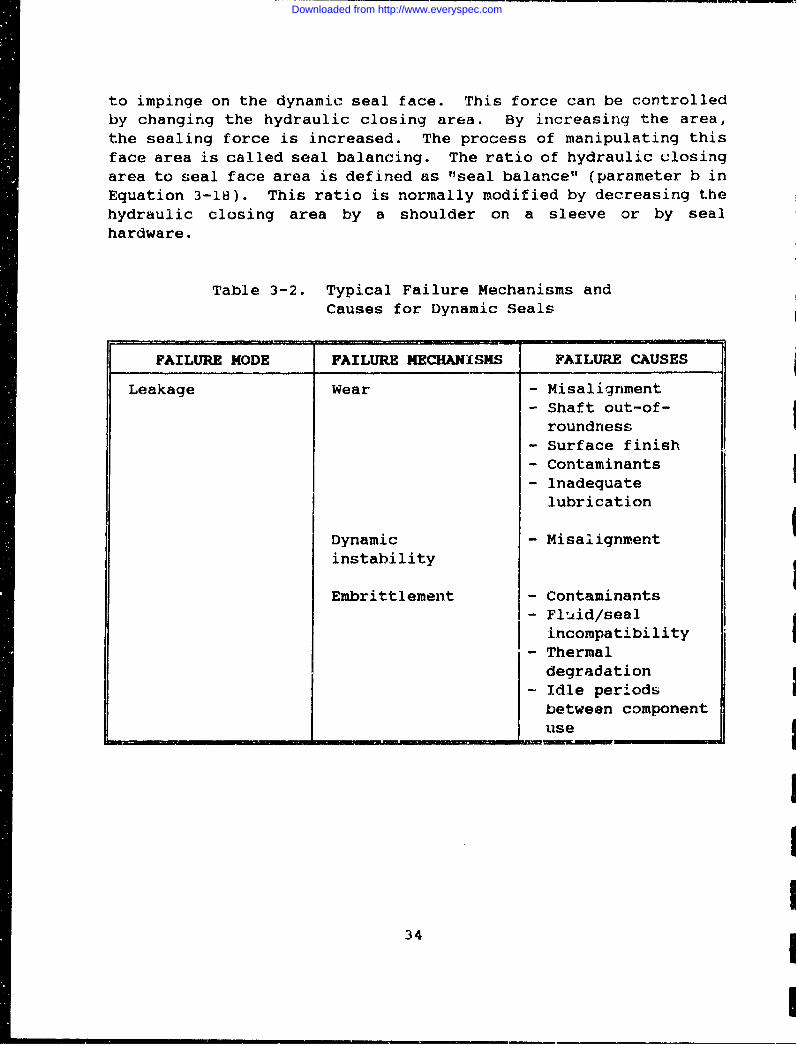
Table 3-2. Typical Failure Mechanisms andCauses for Dynamic Seals

FAILURE MODE FAILURE MECHANISMS FAILURE CAUSES

Leakage Wear - Misalignment- Shaft out-of-

roundness- Surface finish- Contaminants- Inadequate

lubrication

Dynamic - Misalignmentinstability

Embrittlement - Contaminants- Fluid/seal

incompatibility- Thermal

degradation- Idle periods

between componentuse

34


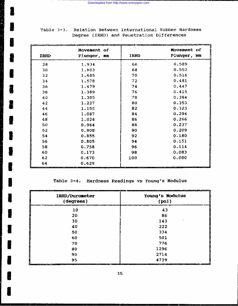
Table 3-3. Relation Between International 'ubber HardnessDegree (IRHD) and Pe•ietration Differences

IMovement of Movement of3R JID Plunger, mm IRHD Plunger, 7m

28 1.934 66 0.58930 1.803 68 0.552I 32 1.685 70 0.51634 1.578 72 0.48136 1.479 74 0.447

38 1.389 76 0.41540 1.305 78 0.38442 1.227 80 0.35344 1.155 82 0,32346 1.087 84 0.294

S48 1.024 86 0.26650 0.964 88 0.23752 0.908 90 0.20954 0.855 92 0.18056 0.805 94 0.15158 0.758 96 0.11460 0.173 98 0.08362 0.670 100 0.000

1 64 0.629

3 BTable 3-4. Hardness Readings vs Young's Modulus

IRHD/Durometer Young's ModulusI (degrees) (psi)

10 4320 8630 14340 222so5 33460 50170 77680 129690 271495 4739

* g35

U


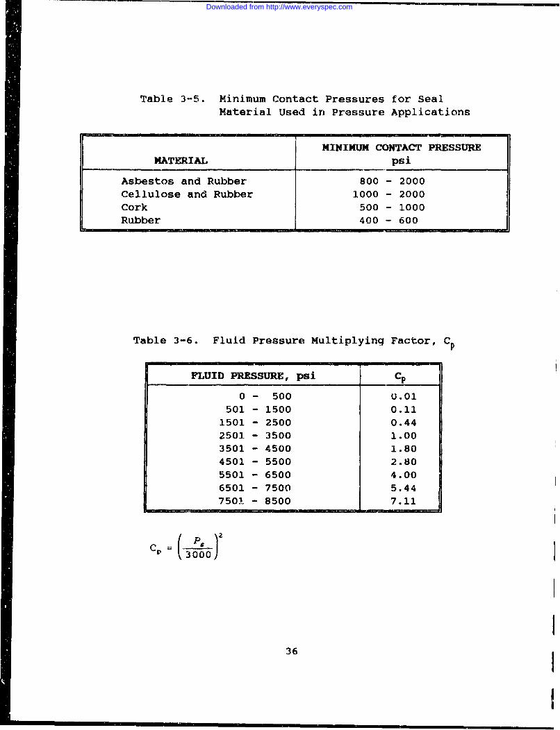
Table 3-5. Minimum Contact Pressures for SealMaterial Used in Pressure Applications

MINIMUM CONTACT PRESSUREMATERIAL psi

Asbestos and Rubber 800 - 2000Cellulose and Rubber 1000 - 2000

Cork 500 - 1000

Rubber 400 - 600

Table 3-6. Fluid Pressure Multiplying Factor, CP

FLUID PRESSURE, psi _ _

0 - 500 0.01501 - 1500 0.11

1501 - 2500 0.44

2501 - 3500 1.003501 - 4500 1.80

4501 - 5500 2.805501 - 6500 4.00

6501 - 7500 5.447501 - 8500 7.11

3000

36


I

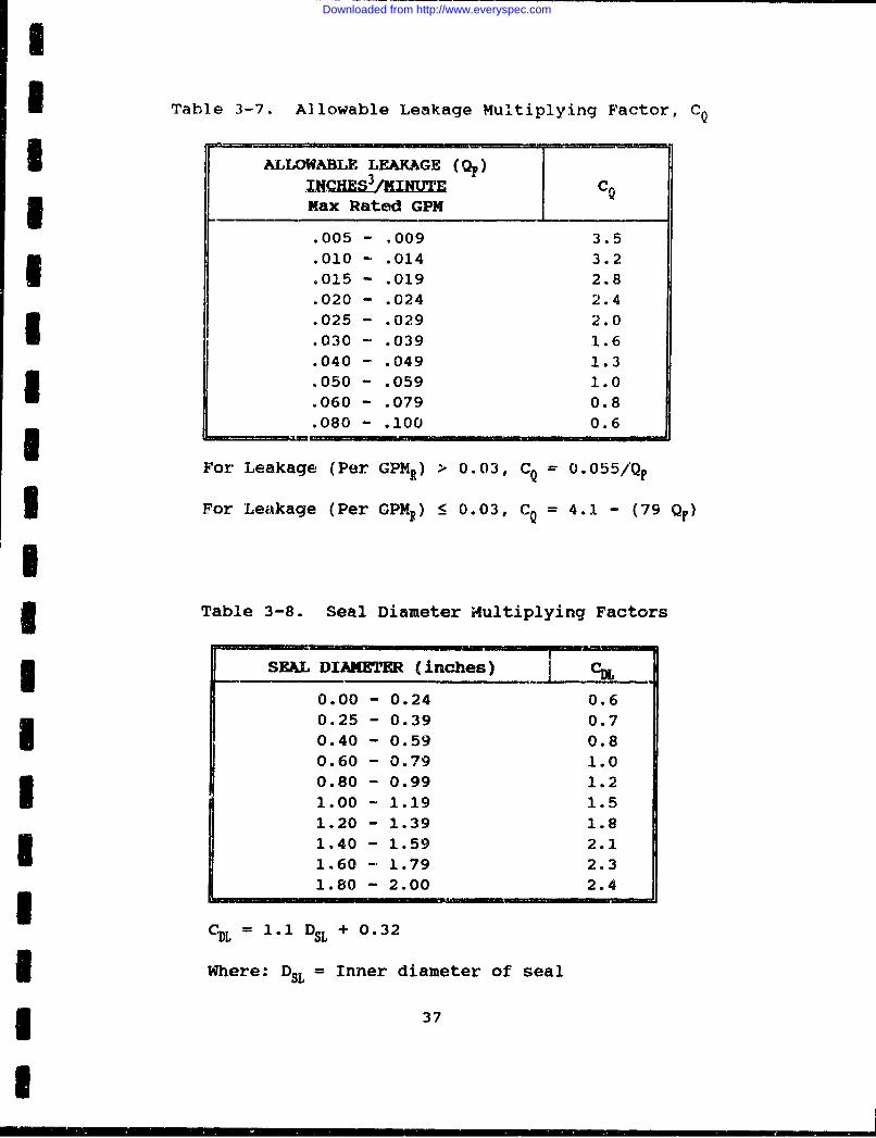
I Table 3-7. Allowable Leakage Multiplying Factor, CQ

ALLOWABLE LEAKAGE (QF)INCHES 3/INUTE c3 Max Rated GPM

.005 - .009 3.5

.010 - .014 3.2

.015 - .019 2.8

.020 - .024 2.4

.025 - .029 2.0

.030 - .039 1.6

.040 - .049 1.33 .050 - .059 1.0.060 - .079 0.8.080 - .100 0.6

F or L II --CUFor Leakage (Per GPMR) > 0.03, CQ = 4.0-5/QF3 For Leakage (Per GPMR) _< 0.03, CQ = 4.1 - (79 QF)

i3 Table 3-8. Seal Diameter Multiplying Factors

SEAL DIAMETER (inches

0.00 - 0.24 0.60.25 - 0.39 0.7

0.40 - 0.59 0.80.60 - 0.79 1.0

0.80 - 0.99 1.2

1.00 - 1.19 1.51.20 - 1.39 1.8

1.40 - 1.59 2.1

1.60 - 1.79 2.31.80 - 2.00 2.4

CDL= 1.1 DSL + 0.32

3 Where: DSL = Inner diameter of seal

37

I


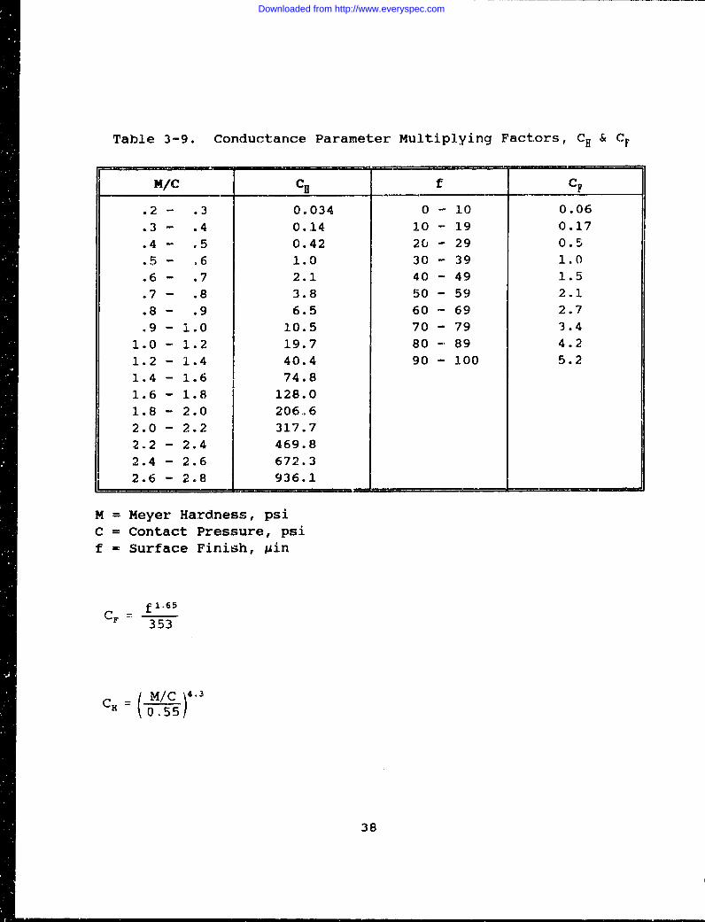
Table 3-9. Conductance Parameter Multiplying Factors, CH & CF

M/C CH f CF

.2 - .3 0.034 0 - 10 0.06

.3 - .4 0.14 10 - 19 0.17

.4 - .5 0.42 20 - 29 0.5

.5- .6 1.0 30 - 39 1.0

.6 - .7 2.1 40 - 49 1.5

.7 - .8 3.8 50 - 59 2.1

.8 - .9 6.5 60 - 69 2.7

.9 - 1.0 10.5 70 - 79 3.4

1.0 - 1.2 19.7 80 - 89 4.2

1.2 - 1.4 40.4 90 - 100 5.2

1.4 - 1.6 74.8

1.6 - 1.8 128.0

1.8 - 2.0 206,6

2.0 - 2.2 317.7

2.2 - 2.4 469.8

2.4 - 2.6 672.3

2.6 - 2.8 936.1

M = Meyer Hardness, psiC = Contact Pressure, psif = Surface Finish, gin

CF f 1.65353

38


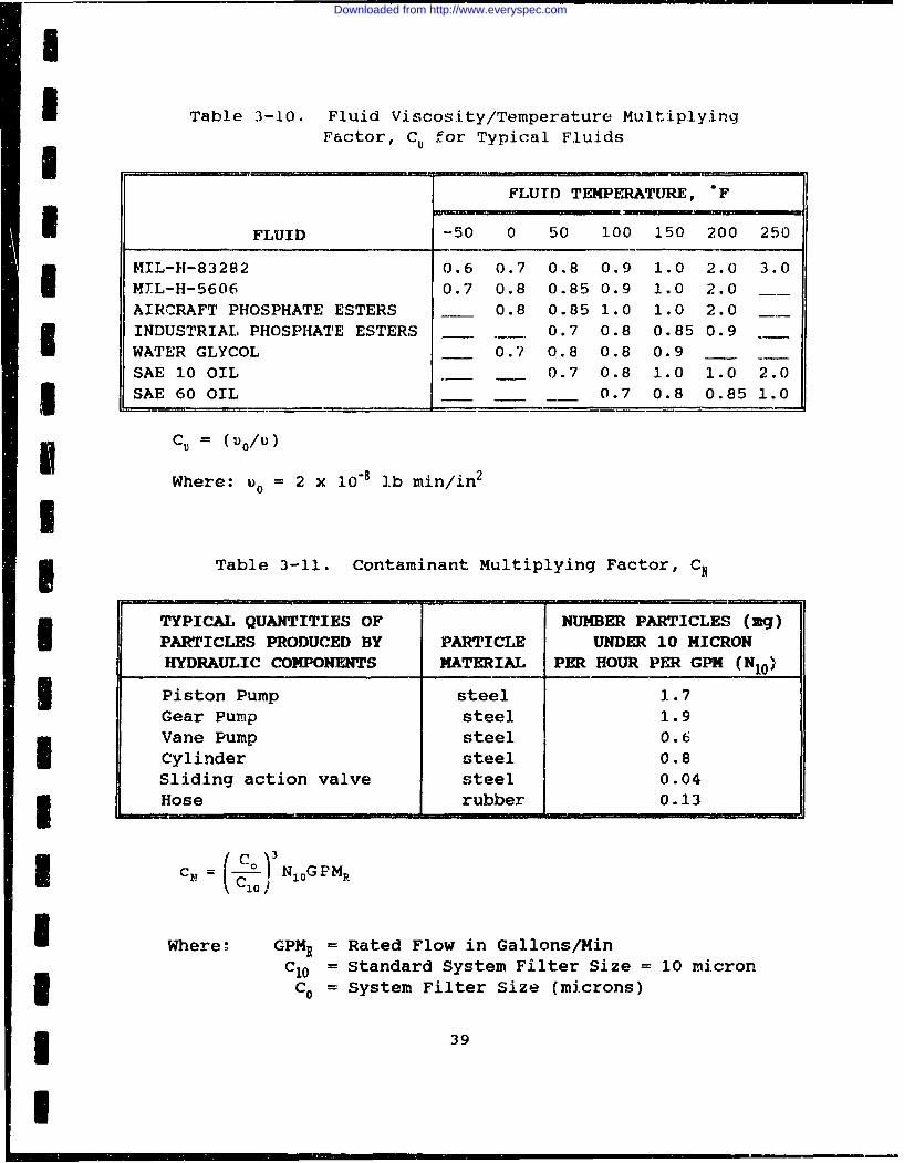
Table 3-10. Fluid Viscosity/Temperature MultiplyingFactor, C0 for Typical Fluids

FLUID TEMPERAT[RE, "F

FLUID -50 0 50 100 150 200 250

MIL-H-83282 0.6 0.7 0.8 0.9 1.0 2.0 3.0MXL-H-5606 0.7 0.8 0.85 0.9 1.0 2.0AIRCRAFT PHOSPHATE ESTERS 0.8 0.85 1.0 1.0 2.0INDUSTRIAL PHOSPHATE ESTERS 0.7 0.8 0.85 0.9WATER GLYCOL 0.7 0.8 0.8 0.9SAE 10 OIL 0.7 0.8 1.0 1.0 2.03 SAE 60 OIL __.0.7 0.8 0.85 1.0

Icu =( )

Where: u0 = 2 x 10-8 ].b min/in2

I Table 3-11. Contaminant Multiplying Factor, CN

TYPICAL QUANTITIES OF NUMBER PARTICLES (mg)PARTICLES PRODUCED BY PARTICLE UNDER 10 MICRONHYDRAULIC COMPONENTS MATERIAL PER HOUR PER GPM (N10 )

Piston Pump steel 1.7Gear Pump steel 1.9Vane Pump steel 0.6

Cylinder steel 0.8Sliding action valve steel 0.043 Hose rubber 0.13

I CN = (IV NlOGPMR

U Where: GPMR = Rated Flow in Gallons/MinC10 = Standard System Filter Size = 10 micron3 C0 = System Filter Size (microns)

* 39

I


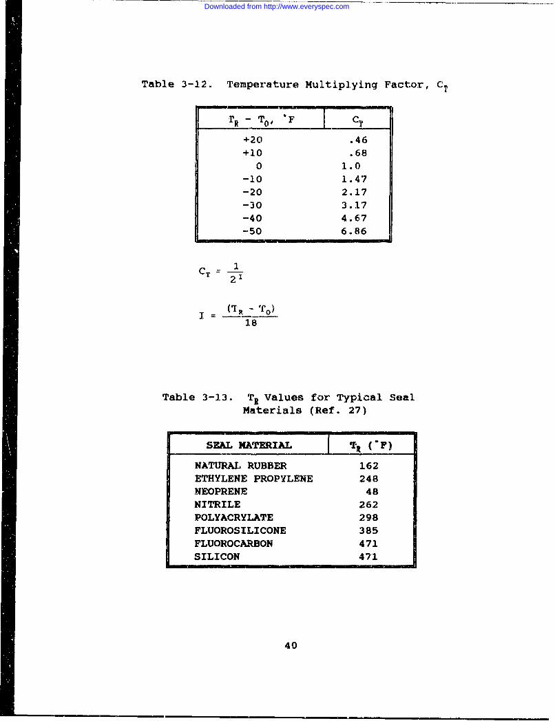
Table 3-12. Temperature Multiplying Factor, CT

TR- To, F CT

+20 .46

+10 .68

0 1.0-10 1.47-20 2.17-30 3.17-40 4.67-50 6.86

CT 12'

= 18

Table 3-13. T, Values for Typical Seal.Materials (Ref. 27)

SEAL MATERIAL IT, C* F)NATURAL RUBBER 162ETHYLENE PROPYLENE 248

NEOPRENE 48NITRILE 262POLYACRYLATE 298FLUOROSILICONE 385

FLUOROCARBON 471

SILICON 471

40


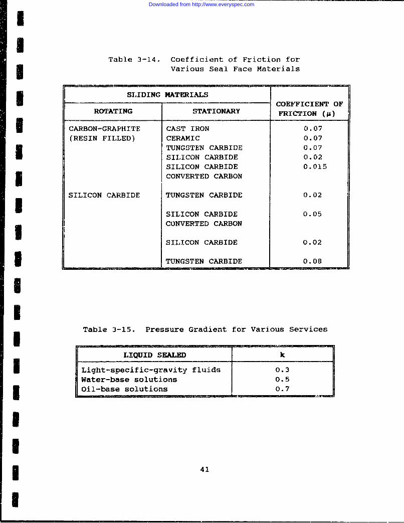
-ITable 3-14. Coefficient of Friction for

Various Seal Face Materia].s

SLIDING MATERIALSCOEFFICIENT OFU ROTATING STATIONARY FRICTION

I CARBON-GRAPHITE CAST IRON 0.07(RESIN FILLED) CERAMIC 0.07

TUNGSTEN CARBIDE 0.07SILICON CARBIDE 0.02

SILICON CARBIDE 0.0153 CONVERTED CARBON

SILICON CARBIDE TUNGSTEN CARBIDE 0.02

SILICON CARBIDE 0.05CONVERTED CARBON

SILICON CARBIDE 0.02

1 TUNGSTEN CARBIDE 0.08

Table 3-15. Pressure Gradient for Various Services

LIQUID SEALED k

I Light-specific-gravity fluids 0.3Water-base solutions 0.5

IOil-base solutions 0.7

II

1 4


THIS PAGE INTENTIONAlLY LEFT BLANK

42


I

CHAPTER 4

SPRINGS

4.1 INTRODUCTIONSprings are provided for many different applications such as

compression, extension, torsion, power, and constant force.Depending on the application, a spring may be in a static, cyclicor dynamic operating mode. A spring is usually considered to bestatic if a change in deflection or load occurs only a few times,such as less than 10,000 cycles during the expected life of thespring. A static spring may remain loaded for very long periods oftime. Cyclic springs are flexed repeatedly and can be expected to

I exhibit a higher failure rate due to fatigue. Dynamic loadingrefers to those occurrences of a load surge inducing higher thannormal stresses on the spring.

I 4.2 FAILURE MODESThe operating life of a mechanical spring arrangement is3 dependent upon the susceptibility of the materials to corrosion and

stress levels (static, cyclic or dynamic). The most common failuremodes for springs are fracture due to fatigue and excessive loss ofload due to stress relaxation. Table 4-1 is a list of failuremechanisms and causes of spring failure. Other failure mechanismsand causes may be identified for a specific application to assurethat all considerations of reliability are included in theprediction. Typical failure rate considerations include: level ofloading, operating temperature, cycling rate and corrosiveenvironment.

If an S 0 value for the spring can be obtained, this value shouldI be used in conjunction with the environmental multiplying factors

contained in this section. The procedure for estimating springfailure rates contained herein is intended to be used in theabsence of specific data.

4.3 FAILURE RATE MODELThe failure rate of a spring depends upon the stress on the

spring and the relaxation provided by the material. The load onthe spring is equal to the spring rate multiplied by the change inload per unit deflection and calculated as follows (Ref. 14):

I43


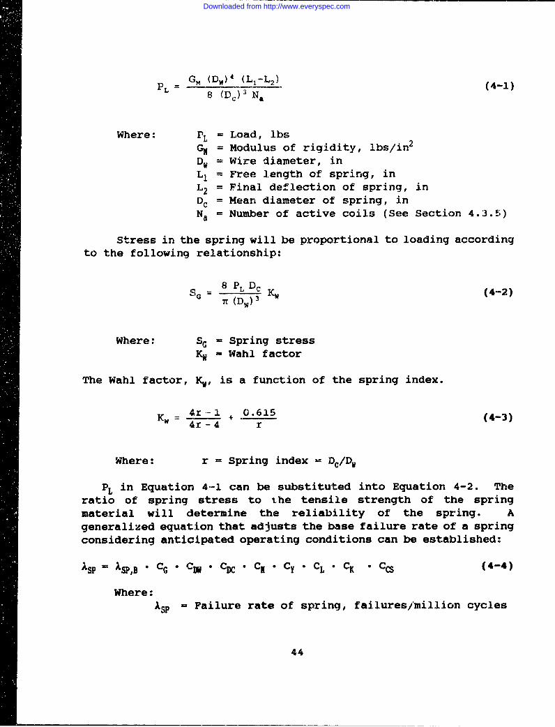
GM (Dy) 4 (L 1 -L 2 ) (4-1)8 (DC) 3 Na

Where: rL = Load, lbsGm = Modulus of rigidity, lbs/in2

DW = Wire diameter, inL1 = Free length of spring, inL2 = Final deflection of spring, inDc = Mean diameter of spring, inNa = Number of active coils (See Section 4.3.5)

Stress in the spring will be proportional to loading accordingto the following relationship:

8 PL Dc (42)

7 (DW) 3

Where: SG= Spring stressKW Wahl factor

The Wahl factor, Kv, is a function of the spring index.

4Z-i 0.615 (43)KW 4r -4 '- r(43

Where: r = Spring index - DC/DV

PL in Equation 4-1 can be substituted into Equation 4-2. Theratio of spring stress to the tensile strength of the springmaterial will determine the reliability of the spring. Ageneralized equation that adjusts the base failure rate of a springconsidering anticipated operating conditions can be established:

ISP = SP,B 0 CG * CDW CDC 0 C * CY * CL * CK C c (4-4)

Where:ASP = Failure rate of spring, failures/million cycles

44


IA SPB = Base failure rate for spring, failures/million

cycles, 0.65 failures/million cyclesCG = Multiplying factor which considers the effect

of the material rigidity modulus on the basefailure rate. See Table 4-2

-CD = Multiplying factor which considers the effect ofthe wire diameter on the base failure rate. SeeTable 4-33CD = Multiplying factor which considers the effect ofcoil diameter on the base failure rate.See Table 4-3

CK = Multiplying factor which considers the effect ofthe number of active coils on the base failure

3 rate. See Table 4-3CY = Multiplying factor which considers the effect of

material tensile strength on the base failurerate. See Table 4-4I CL = Multiplying factor which considers the effect ofspring deflection on the base failure rate.See Table 4-5

CK = Multiplying factor which includes the springconcentration factor and the Wahl factor.3 iSee below and Table 4-6

JCC = Multiplying factor which considers the effect ofspring cycle rate on the base failure rate.I See below.

CK, the spring stress concentration factor, is a function of theI Wahl factor, K. which is a function of the spring index. Valuesfor CK are provided in Table 4-6 in terms of the spring index.

iCC, the spring cycle rate factor, has been initially derivedfrom data given by (Ref.12). If the cycle rate is less than 300cycles per minute, CC is 1.0. If the cycle rate is between 300 and360 cycles per minute, C3 is 6.0. For rates above 360 cycles perminute, Cs is estimated to be 12.0.

The parameters in the failure rate equation can be located on anengineering drawing by knowledge of design standards or by actualmeasurement. Other manufacturing, quality, and maintenanceScontributions to failure rate are included in the base failure rateas determined from field performance data. The followingFparagraphs provide background information on those parametersincluded in Equation (4-4).

I i45


I

4.3.1 tacSpriungjiStatic springs can be used in constant deflection or constant

load applications. A constant deflection spring is cycled througha specified deflection range, the loads on the spring causing some Iset or relaxation which in turn lowers the applied stress. Thespring may relax with time and reduce the applied load. Underconstant load conditions, the load applied to the spring does not.change during operation. Constant load springs may set or creep,but the applied stress is constant. The constant stress may result 3in fatigue lives shorter than those found in constant deflectionapplications. The failure rate model included in this section wasderived for cyclic springs. The base failure rate can be used asan approximate value for static springs.

4.3.2 !9injjg-prjngsiCyclic springs can be classified as being unidirectional or

reverse loaded. In one case, the stress is always applied in thesame direction, while in the other, stress is applied first in one Idirection then in the opposite direction.

4.3.3 H]d)j13qRiRg• it.• yThe modulus of rigidity provides a measure of elasticity in

shear for the spring material. Values are provided in Table 4-2.

4.3.4 SpringXSpring index (r) is the ratio of mean coil diameter to wire 3

diameter. A spring with a high index will tend to tangle orbuckle. Modification factors for spring coil diameter and wirediameter are provided in Table 4-3. 34.3.5 _mb ofL Active Coils

The number of active coils is usually two less than the total inumber of coils. There is some activity in the end coils, butduring deflcction, some active material comes in contact with theend coils and becomes inactive. Therefore, the total number of Icoils minus two is a good approximation for the number of activecoils. Modification factors for the number of coils are providedin Table 4-3.

4.3.6 T-emile StnThe tensile strengcu prcvides a measure of spring material

deformation or set as a function of stress. Values of tensilestrength are included in Table 4-4.

46strenth ar


I4.3.7

"If the spring has a variable diameter such as occurs forconical, barrel and hourglass springs, the spring can be dividedanalytically into smaller increments and the failure ratec•lculated for each. The failure rate for the total spring iscoml[uted by adding the rates for the increments.

4.3. 8 Corr~zimnI nThe reliability of a spring in terms of fatigue life andload-carrying ability will be affected by corrosion, the quan--itative effect being very hard to predict. Springs are almostI always in contact with other metal parts. If a spring is to besubjected to a corrosive environment, the use of inert materialsprovides the best defense against corrosion. Protective coatingsI can also be applied. The spring material is normally more noble(chemically resistant to corrosion) than the structural componentsin contact with ý.t because the lesser noble alloy will be attackedby the electrolyte. The effects of corrosion on spring reliabilityare included in the base failure rate. This rate may have to be3 Hadjusted based on experience data considering the extent of acorrosive environment.

S4.3.9 Other Reliability Considerations for .sZrngsThe most common failure modes of springs include fracture due to

fatigue and excessive loss of load. A reliability analysis shouldI include a review of the following items to assure maximum, possiblelife.

- Sharp corners and similar stress risers should beI minimized.* The hardness of the spring material can be sensitive

to plating and baking operations. Quality controlprocedures for these operations should be reviewed.

• When a spring is loaded or unloaded, a surge wavemay transmit torsional stress to the point of restraint.The impact velocity should be determined to assure thatthe maximum load rating of the spring is not exceeded.

• Operating temperature should be determined. Both highand low temperature conditions may require considerationof specialized materials.I *Exposure to electrical fields which may magnetize '%.hespring material.

* |47

I


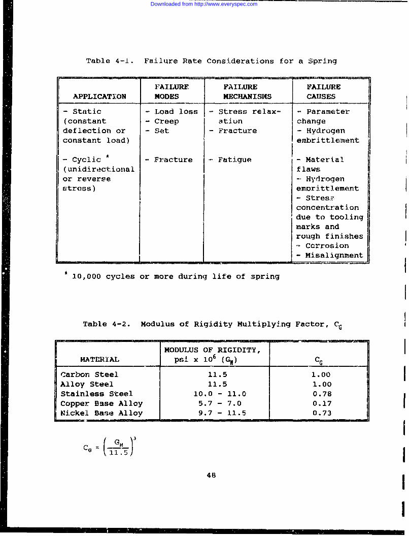
Table 4-1. Failure Rate Considerations for a Spring

FAILURE FAIIURE FAILURE"APPLICATION MODES MECHAN I SMS CAUSES

- Static - Load loss - Stress relax- - Parameter(constant - Creep atiun changedeflection or - Set - Fracture - Hydrogenconstant load) embrittlement

- Cyclic - Fracture Fatigue - Material(unidirectional flawsor reverse - Hydrogenstress) emorittlement

- StresFconcentration

due to toolingmarks andrough finishes

Ccrrosion- Misalignment

10,000 cycles or more during life of spring

Table 4-2. Modulus of Rigidity Multiplying Factor, CG

MODULUS OF RIGIDITY,MATERIAL psi x 106 (Gý) CG

Carbon Steel 11.5 1.00Alloy Steel 11.5 1.00Stainless Steel 10.0 - 11.0 0.78Copper Base Alloy 5.7 - 7.0 0.17Nickel Base Alloy 9.7 - 11.5 0.73

CG r (_2j_5c ,11.5]

48

IF I I• .. .


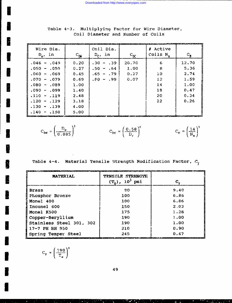
I

I Table 4-3. Multiplying Factor for Wire Diameter,Coil Diameter and Number of Coils

Wire Dia. Coil Dia. # ActiveDw, in C DC, in C Coils Na CH

.046 - .049 0.20 .30 - .39 20.70 6 12.70

.050 - .059 0.27 .50 - .64 1.00 8 5.36

.060 - .069 0.45 .65 - .79 0.27 10 2.74

.070 - .079 0,69 .80 - .99 0.07 12 1.59

.080 - .089 1.00 14 1.00

.090 - .099 1.40 18 0.47

.110 - .119 2.48 20 0.34

I.120 - .129 3.18 22 0.26

.130 - .139 4.00

.140 - .150 5.00

CD = 8 14 :IC0x 0.085 CDC jO--- CMD (, &

ITable 4-4. Material Tensile Strength Modification Factor, Y

MATERIAL TENSILE STRENGIT(TS)_, 103 psi C _

Brass 90 9.40Phosphor Bronze 100 6.86Monel 400 100 6.86Inconel 600 150 2,03Monel K500 175 1.28Copper-Beryllium 190 1.00

Stainless Steel 301, 302 190 1.0017-7 PH RH 950 210 0.90Spring Temper Steel 245 0.47

* 49

I


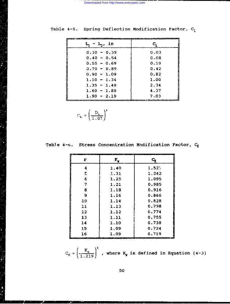
Table 4-5. Spring Deflection Modification Factor, CL

-L2 in CL

F 0.30 - 0.39 0.030.40 - 0.54 0.08

0.55 - 0.69 0.19

0.70 - 0.89 0.42

0.90 - 1.09 0.82

1.10 - 1.34 1.00

1.35 - 1.49 2.34

1.60 - 1.89 4.37

1.90 - 2.19 7.03

CL DL )3(1.07)

Table 4-6. Stress Concentration Modification Factor, CK

r IN CK4 1.40 1.52*5 1.31 1.2426 1.25 1.095

7 1.21 0.9858 1.18 0.9169 1.16 0.866

10 1.14 0.82811 1.13 0.79812 1.12 0.77413 1.11 0.75514 1.10 0.73815 1.09 0.72416 1.09 0.719

C= , where Kw is defined in Equation (4-3)

50


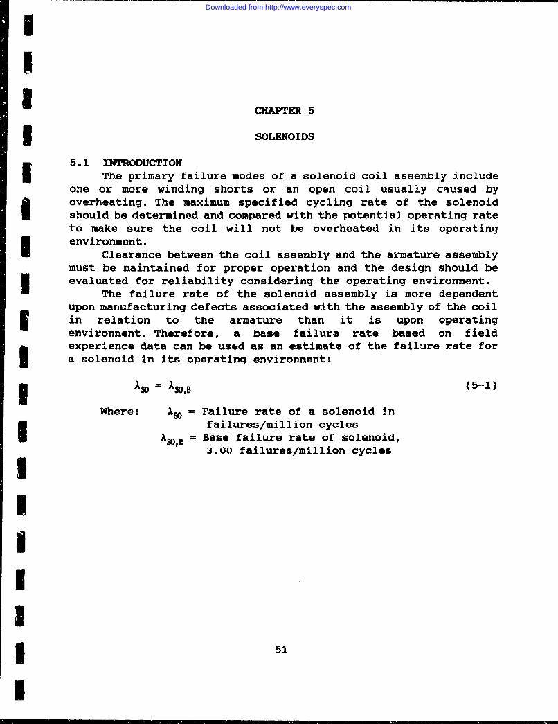
I

CHAPTER 5

5i SOLENOIDS

5.1 INTRODUCTION5 The primary failure modes of a solenoid coil assembly includeone or more winding shorts or an open coil usually cnused byoverheating. The maximum specified cycling rate of the solenoid

Sshould be determined and compared with the potential operating rateto make sure the coil will not be overheated in its operatingenvironment.

Clearance between the coil assembly and the armature assemblymust be maintained for proper operation and the design should beevaluated for reliability considering the operating environment.

The failure rate of the solenoid assembly is more dependentupon manufacturing defects associated with the assembly of the coil3 in relation to the armature than it is upon operatingenvironment. Therefore, a base failure rate based on fieldexperience data can be used as an estimate of the failure rate fora solenoid in its operating environment:

Aso X SOB (5-1)

Where: IS= Failure rate of a solenoid infailures/million cycles

,B = Base failure rate of solenoid,3.00 failures/million cycles

3mIII

I



52


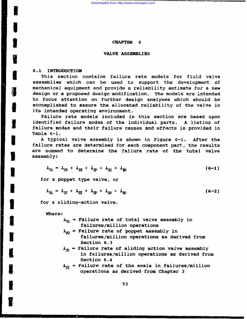
II

3 CHAPTER 6

w VALVE ASSEMBLIES

6.1 INTRODUC`TIONThis section contains failure rate models for fluid valve

assemblies which can be used to support the development ofmechanical. equipment and provide a reliability estimate for a newdesign or a proposed design modification. The models are intendedto focus attention on further design analyses which should beI accomplished to assure the allocated reliability of the valve inits intended operating environment.

Failure rate models included in this section are based uponidentified failure modes of the individual parts. A listing offailure modes and their failure causes and effects is provided inTable 6-1.

A typical valve assembly is shown in Figure 6-1. After thefailure rates are determined for each component part, the resultsare summed to determine the failure rate of the total valveI assembly:

AVA = PO + ASE + ASP + Aso 4 ABO (6-1)

for a poppet type valve, or

I ~ VA=V +ISE+ SP+Aso+IBO (6-2)

3 for a sliding-action valve.

Where:

Wr VA = Failure rate of total valve assembly infailures/million operations

-A - Failure rate of poppet assembly in3% failures/million operations as derived fromSection 6.3

1= Failure rate of sliding action valve assemblyin failures/million operations as derived fromSection 6.4

ISE = Failure rate of the seals in failures/millionoperations as derived from Chapter 3

153


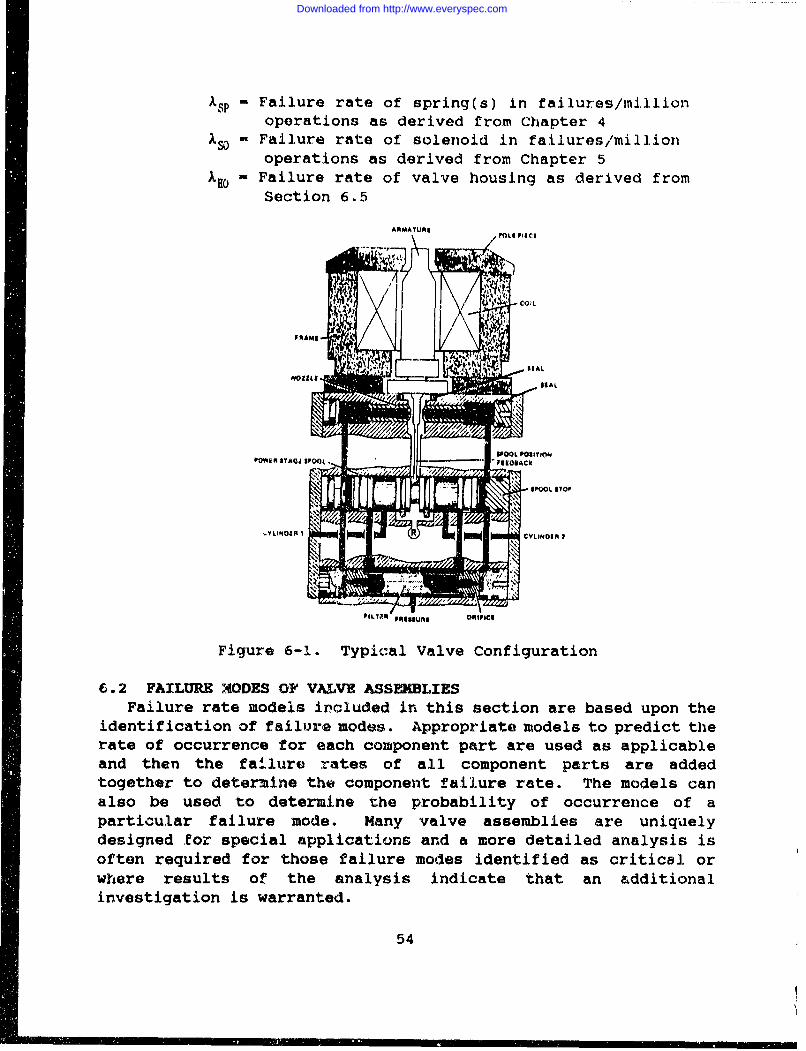
Isp - Failure rate of spring(s) in failures/millionoperations as derived from Chapter 4

I- Failure rate of solenoid in failures/millionoperations as derived from Chapter 5

IBO- Failure rate of valve housing as derived fromSection 6.5

AftIMA YuR|

, .LI PIECE

/ iS• COýL

FAAM1.NOZZ•• • HAL

&POOL POSITION•POWER ITAOQJ SPO"- P0iON&c

Pi RINS MsUi ORIFICI

Figure 6-I. Typical Valve Configuration

6.2 FAILURE MODES OF VALVE ASSFBLIESFailure rate models included in this section are based upon the

identification of failure modes. Appropriate models to predict tiherate of occurrence for each component part are used as applicableand then the failure rates of all component parts are addedtogether to determine the component failure rate. The models canalso be used to determine the probability of occurrence of aparticular failure mode. Many valve assemblies are uniquelydesigned for special applications and a more detailed analysis isoften required for those failure modes identified as critical orwhere results of the analysis indicate that an additionalinvestigation is warranted.

54


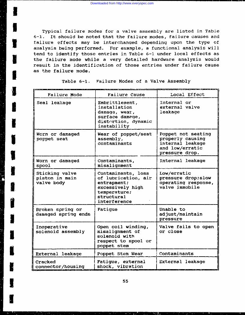
I

Typical failure modes for a valve assembly are listed in Table6-1. It should be noted that the failure modes, failure causes andI failure effects may be interchanged depending upon the type ofanalysis being performed. For example, a functional analysis will.tend to identify those entries in Table 6-1 under local effects asthe failure mode while a very detailed hardware analysis wouldresult in the identification of those entries under failure cause

* as the failure mode.

'Table 6-1. Failure Modes of a Valve Assembly

Failure Mode Failure Cause Local Effect

Seal leakage Embrittlement, Internal orinstallation external valvedamage, wear, leakagesurface damage,distnrtion, dynamic

__instability

Worn or damaged Wear of poppet/seat Poppet not seatingpoppet seat assembly, properly causing

contaminants internal leakageand low/erratic

___...pressure drop.

Worn or damaged Contaminants, Internal leakagespool misalignment

Sticking valve Contaminants, loss Low/erraticpiston in main of lubrication, air pressure drop;slowvalve body entrapment; operating response,

excessively high valve immobilea 'temperature;

structuralinterference

Broken spring or Fatigue Unable todamaged spring ends adjust/maintain

pressure

Inoperative Open coil winding, Valve fails to opensolenoid assembly misalignment of or closeU solenoid with

respect to spool or_ _ _ _ poppet stem

External leakage Poppet Stem Wear Contaminants

Cracked Fatlgue, external External leakageconnector/housing j shock, vibration I

*55


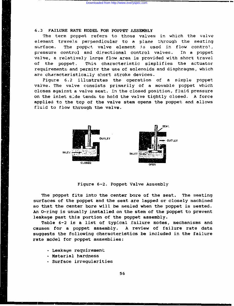
6.3 FAILURE RATE H'ODEL FOR POPPET hSSEMBLYThe term poppet refers to those valves in which the valve

element travels perpendicular to a plane through the seatingsurface. The poppet valve element is used in flow control,pressure control and directional control valves. In a poppetvalve, a relatively larqe flow area is provided with short travelof the poppet. This characteristic simplifies the actuatorrequirements and permits the use of solenoids and diaphragms, whichare characteristically short stroke devices.

Figure 6.2 illustrates the operation of a simple poppetvalve. The valve consists primarily of a movable poppet whichcloses against a valve seat. In the closed position, fluid pressureon the inlet side tends to hold the valve tightly closed. A forceapplied to the top of the valve stem opens the poppet and allowsfluid to flow through the valve.

OUUTLET

INLE

LE

CLOSED OE

Figure 6-2. Poppet Valve Assembly

The poppet fits into the center bore of the seat. The seatingsurfaces of the poppet and the seat are lapped or closely machinedso that the center bore will be sealed when the poppet is seated.An 0-.ring is usually installed on the stem of the poppet to preventleakage past this portion of the poppet assembly.

Table 6-2 is a list of typical failure modes, mechanisms andcauses for a poppet assembly. A review of failure rate datasuggests the following characteristics be included in the failurerate model for poppet assemblies:

"* Leakage requirement"* Material hardness"• Surface irregularities

56


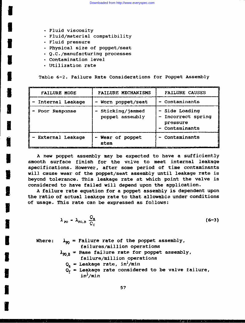
I

U • Fluid viscosity• Fluid/material compatibility• Fluid pressure6 Physical size of poppet/seat. Q.C./Imanufacturing processes3 *Contamination level. Utilization rate

3 Table 6-2. Failure Rate Considerations for Poppet Assembly


- Internal Leakage - Worn poppet/seat - Contaminants

I - Poor Response - Sticking/jammed - Side Loadingpoppet assemably - Incorrect spring

pressure- Contaminants

- External Leakage - Wear of poppet - Contaminantsstem I

A new poppet assembly may be expected to have a sufficientlysmooth surface finish f or the valve to meet internal leakagespecifications. However, after some period of time contaminantswill cause wear of the poppet/seat assembly until leakage rate isbeyond tolerance. This leakage rate at which point the valve isconsidered to have failed will depend upon the application.3 A failure rate equation for a poppet assembly is dependent uponthe ratio of actual leakege rate to that allowable under conditionsof usage. This rate can be expressed as follows:

3 XPO .PO.B Q (6-3)

3 Where: 4 Failure rate of the poppet assembly,failures/million operations

,_P0,B = Base failure rate for poppet assembly,failure/million operations

Qa= Leakage rate, in3/miinQf = Leakage rate considered to be valve failure,

in 3/min

3 57

I • i• ; " , -m! -• I r •' m •• •


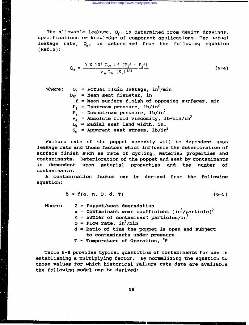
The allowable leakage, Qf, is determined from design drawings,specifications or knowledge of component applications. The actualleakage rate, Qa' is determined from the following equation(Ref.5):

Qa 2 X 10 DMS f 1 (PI 2 - - (6-4) SVa L W (S") 3/2

Where: Qa= Actual fluid leakage, in 3/minSDy= Mean seat diameter, in

f = Mean surface f..nish of opposing surfaces, minP1 = Upstream pressure, lb/in2

P2 = Downstream pressure, ib/in2Va = Absolute fluid viscosity, lb-min/in2

LW = Radial seat land width, in.S = Apparent seat stress, lb/in2

Failure rate of the poppet assembly will be dependent uponleakage rate and those factors which influence the deterioration ofsurface finish such as rate of cycling, material properties andcontaminants. Deterioration of the poppet and seat by contaminantsis dependent upon material properties and the number ofcontaminants.

A contamination factor can be derived from the followingequation:

2 = f(a, n, Q, d, T)(-}

Where: Z = Poppet/seat degradationa = Contaminant wear coefficient (in 3/particle) 2

n = number of contaminant' particles/in3

Q = Flow rate, in 3/mind = Ratio of time the poppet. is open and subject

to contaminants under] pressureT = Temperature of Operation, OF

Table 6-8 provides typical quantities of contaminants for use inestablishing a multiplying factor. By normalizing the equation tothose values for which historical ZaiLure rate data are availablethe following model can be derived:

58


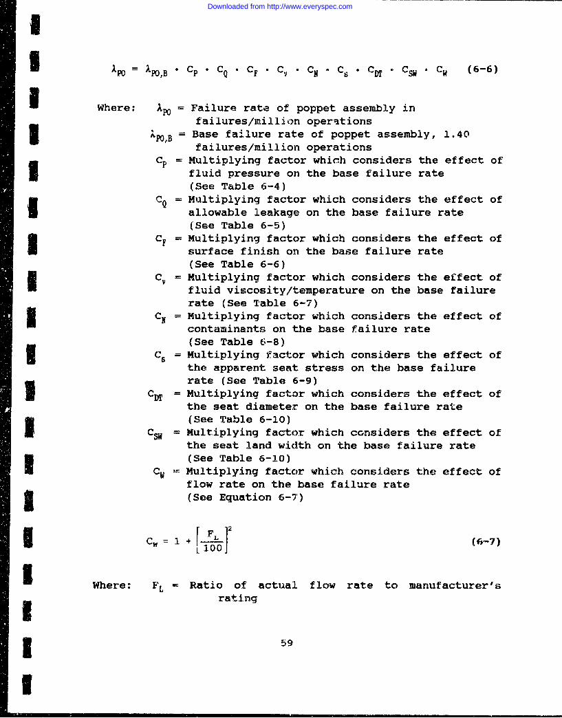
IPO = xP,B •Cp C Q * CF • Cv • CN - Cs • CD • CSW , CW (6-6)

Where: AP= Failure rate of poppet assembly in

failures/million operationsmI ,POB = Base failure rate of poppet assembly, 1.40

failures/million operationsC = Multiplying factor whichk considers the effect ofI fluid pressure on the base failure rate

(See Table 6-4)CQ = Multiplying factor which considers the effect ofI allowable leakage on the base failure rate

(See Table 6-5)CF = Multiplying factor which considers the effect ofI surface finish on the base failure rate

(See Table 6-6)Cv = Multiplying factor which considers the effect of

fluid viscosity/temperature on the base failurerate (See Table 6-7)

C= Multiplying factor which considers the effect ofcontaminants on the base failure rate(See Table 6-8)

Cs = Multiplying factor which considers the effect ofthe apparent seat stress on the base failurerate (See Table 6-9)ICD = Multiplying factor which considers the effect ofthe seat diameter on the base failure rate(See Table 6-10)IC• = Multiplying factor which considers the effect ofthe seat land width on the base failure rate(See Table 6-10)

CW = Multiplying factor which considers the effect offlow rate on the base failure rate3 (See Equation 6-7)

CW + 1 _I00] (6-7)

I Where: FL Ratio of actual flow rate to manufacturer's

rating

SI 59

-I


The following paragraphs provide background information on thoseparameters included in the model.

6.3.1 Fluid PressureTable 6-4 contains the fluid pressure multiplying factors for

use in the model. Valves having high response characteristics aridonsequently a high poppet velocity will incur large seat stresses

which tend to reduce the life expectancy of the valve. As with anypiece of mechanical equipment, the higher the structural loads the Ishorter the life. Pressure forces arise from any net pressureunbalance acting on the valve element. Depending upon thefunctional design of the valve, the pressure force may increase,decrease, or virtually have no effect on the actuation force. Inan unbalanced valve design such as a conventional poppet, upstreampressure ncrmally acts in a direction to seat the valve so that anincreasing upstream pressure will tend to force the valve elementtighter against its seat. The use of pressure unbalance to aid insealing requires a higher actuation force to open the valve. Whenthe size of thc valve and the magnitude of pressure demandexcessively large actuation forces, a balanced design and/orpiloting is often utilized. In most cases the pressure on thepoppet, P. can be a3sumed to be the system upstream pressure, P,'minus the downstream pressure, P2.

6.3.2 Allowable LeakaggTable 6-5 contains the allowable leakage multiplying factor for

use in the model. Allowable internal leakage of a poppet designcan be obtained from valve specifications. Leakage requirementsvary from molecular flow for certain shutoff valves at one extremeto several cubic feet per minute in scme inexpensive valves whichcontrol water or other inexpensive fluid. Allowable leakage mustbe evaluated with respect to total mission and operationalrequirements.

6.3.3 Contamination SensitivityCleanliness of the system and of the fluid medium has a direct

effect upon the operation ano life of a poppet valve. Contaminantscan clog or jam the poppet and cause excessive leakage in Imetal-to-metal seated valves. Particulate matter in gaseous media,especially in the lighter gases such as helium, can be extremelydestructive to internal parts, particularly seats, because of thevery high velocity that can be attained under sonic conditions.

The analysis of particle sizes includes the determination of

60


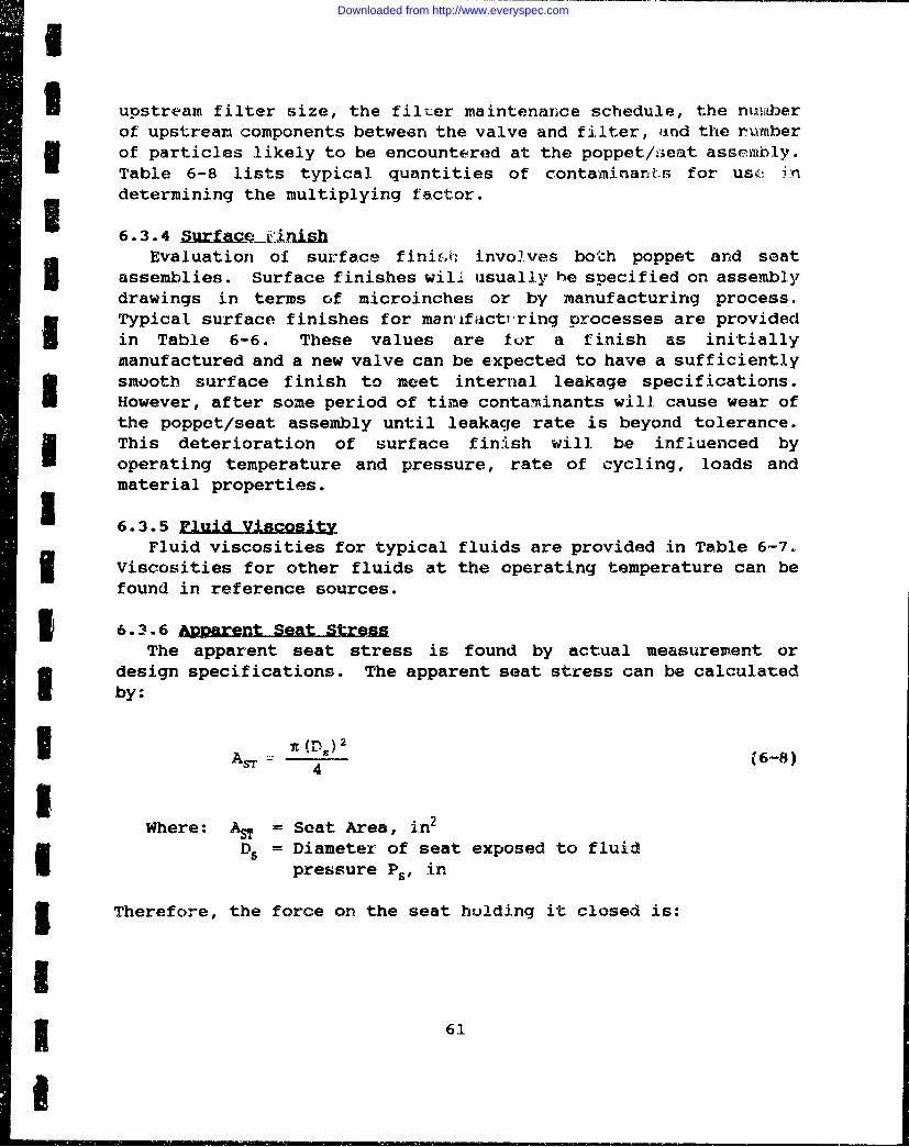
I upstream filter size, the filter maintenance schedule, the nuvb)erof upstream components between the valve and filter, ind the r~uberof particles likely to be encountered at the poppet/8;eat assembly.Table 6-8 lists typical quantities of contaminants for us 'indetermining the multiplying factor.

6.3.4 S-!rLiin1hEvaluation of surface fini.;i involves both poppet and seatI assemblies. Surface finishes will usually he specified on assembly

drawings in terms of microinches or by manufacturing process.Typical surface finishes for manlifact, ring processes are providedI in Table 6-6. These values are for a finish as initiallymanufactured and a new valve can be expected to have a sufficientlysmooth surface finish to meet internal leakage specifications.I However, after some period of time contaminants will cause wear ofthe poppet/seat assembly until leakage rate is beyond tolerance.

*i This deterioration of surface finish will be influenced byoperating temperature and pressure, rate of cycling, loads andmaterial properties.

I 6.3.5 sityFluid viscosities for typical fluids are provided in Table 6-7.

Viscosities for other fluids at the operating temperature can befound in reference sources.

S 6.3.6 Ap•eznt Seat StressThe apparent seat stress is found by actual measurement or

design specifications. The apparent seat stress can be calculatedby:

I • (Dr)AST 4 (6-8)i4

Where: S = Seat Area, in 2

Ds Diameter of seat exposed to fluidpressure Ps, in

3 lTherefore, the force on the seat holding it closed is:

I1 6


,c PQ DO (6--9)" 4

The seat area acting as a t•eal when the valve is closed iscalculated by:

ASL = ,DX IW (6-10) 1Where: ASL = Seat land area, in 2

LW = Land airea width, inD= Mean land width diameter, in

Then the expression for the apparent seat stress S becomes-

=- Force on Seat FE (6-11)Seat Land Area ASL I

Therefore: I

s P Do2 (6-12)4 DM Lw

The minimum contact stress to prevent leakage for most materialeis approximately three times the fluid pressure. I

Therefore, Minimum Contact Pressure = Sc = 3Ps (6-13)

A ratio of minimum contact pressure and the apparent seat stresscan be used as an expression for the stress on a valve to causeleakage:

Stress Ratio = SC/SS = SR (6-14)

In Equation (6-4), leakage varies with the seat stress as:

( )3/2

621


I

3 Therefore, a multiplying factor for tne effect of seat stress onthe valve base failure rata can be expressed:

c (6-15)iU. SR 1,

3 Where:

R 12 71 LW 111D02

Table 6-9 lists the multiplying factors for different values ofseat stress.

6.3.7 •0The seat diameter, D., is approximately equal to the inside

i diameter of the connecting pipe or tubing and this dimension aswell as the land width of the seat, LV, can be obtained orestimated from engineerinq drawings. T&Vh1e 6-10 lists the

I multiplying factors for seat diameter and land width.

6. 3. 8 QPrt-nTM AtrThe duty cycle of a poppet valve can vary from several on-off

cycles to many hundreds of cycles per hour. Multiple cycling underhigh pressure or operating temperature decreases the life of thevalve. The rate of cycling may be important if the temperaturerise, as a result of the operation, becoines significant. Theeffects of fluid temperature on failure rate are included in thefluid viscosity multiplying factor, C,.

6.3,.9 Qetoer C9sdvra•tj9Several failure rate considerations are not specifically

included in the model but rather incli'ded in the base failurerate. The base failure rate is an average value which reflectsfield performance data. The following items can be used as a checklist to assure that the potential failure mechanisms have beenconsidered:

SFluid medium considerations which are important in valve

designs include the physical properties of tha fluid and thecompatibility of the fluid with poppet/seat materials. Corrosive

3 63

Im


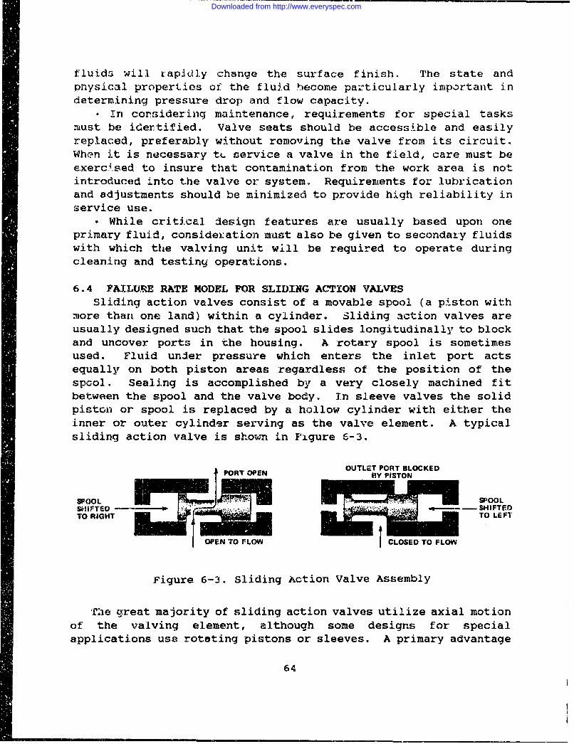
fluids will x:apldly change the surface finish. The state andpnysical properties of the fluid become particularly important indetermining pressure drop and flow capacity.

• In corsidering maintenance, requirements for special tasksmust be ider'tified. Valve seats should be accessible and easilyreplaced, preferably without removing the valve from its circuit.When it is necessary tL service a valve in the field, care must beexercised to insure that contamination from the work area is notintroduced into the valve or system. Requirements for lubricationand adjustments should be minimized to provide high reliability inservice use.

• While critical design features are usually based upon oneprimary fluid, considexation must also be given to secondary fluidswith which the valving unit will be required to operate duringcleaning and testing operations.

6.4 FAILURE RATE MODEL FOR SLIDING ACTION VALVESSliding action valves consist of a movable spool (a piston with

more than one land) within a cylinder. Sliding action valves areusually designed such that the spool slides longitudinally to blockand uncover ports in the housing. A rotary spool is sometimesused. Fluid under pressure which enters the inlet port actsequally on both piston areas regardless of the position of thespool. Sealing is accomplished by a very closely machined fitbetween the spool and the valve body. In sleeve valves the solidpiston or spool is replaced by a hollow cylinder with either theinner or outer cylinder serving as the valve element. A typicalsliding action valve is shown in F'gure 6-3.

OUTLET PORT BLOCKED

1PORT OPEN BY PISTON

SPOOL ME SPOOLSIiFTED -SH I.,F ' . .-- S4 IF TEDTO RIGHT TO LEFT

C 7 iEN ;TO FLOW CLOSED TO FLOW

Figure 6-3. Sliding Action Valve Assembly

The great majority of sliding action valves utilize axial motionof the valving element, although some designs for specialapplications use rotating pistons or sleeves. A primary advantage

64


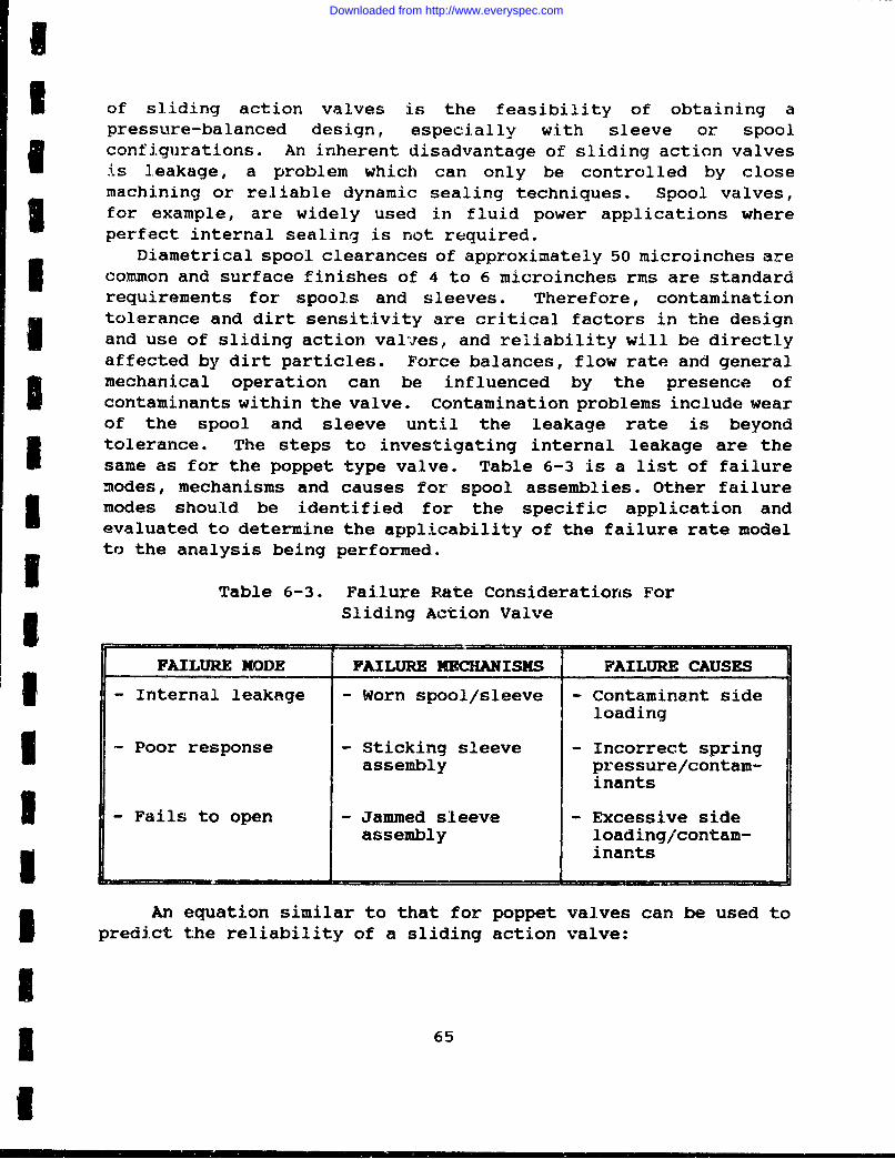
I of sliding action valves is the feasibility of obtaining apressure-balanced design, especially with sleeve or spoolconfigurations. An inherent disadvantage of sliding action valvesis leakage, a problem which can only be controlled by closemachining or reliable dynamic sealing techniques. Spool valves,for example, are widely used in fluid power applications whereperfect internal sealing is not required.

Diametrical spool clearances of approximately 50 microinches arecommon and surface finishes of 4 to 6 microinches rms are standardrequirements for spools and sleeves. Therefore, contaminationtolerance and dirt sensitivity are critical factors in the designand use of sliding action valves, and reliability will be directlyaffected by dirt particles. Force balances, flow rate and generalmechanical operation can be influenced by the presence ofcontaminants within the valve. Contamination problems include wearof the spool and sleeve until the leakage rate is beyondtolerance. The steps to investigating internal leakage are thesame as for the poppet type valve. Table 6-3 is a list of failuremodes, mechanisms and causes for spool assemblies. Other failureK modes should be identified for the specific application andevaluated to determine the applicability of the failure rate modelto the analysis being performed.

Table 6-3. Failure Rate Considerations Forg _Sliding Action Valve


- Internal leakage - Worn spool/sleeve - Contaminant sideloading

Poor response - Sticking sleeve - Incorrect spring

assembly pressure/contam-inants

I - Fails to open - Jammed sleeve - Excessive sideassembly loading/contam-U _inants

An equation similar to that for poppet valves can be used topredict the reliability of a sliding action valve:

6

3 6


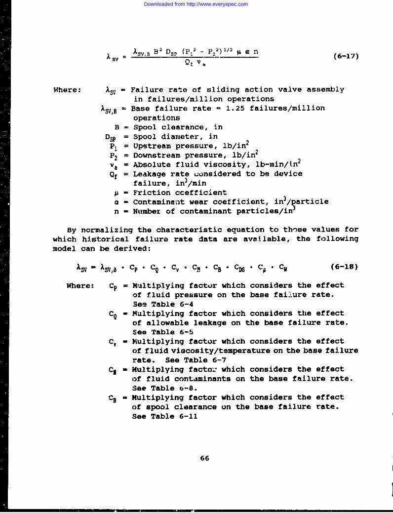
.SVB B 2 Dsp (P. 2 - P 22 )1/2 g a n=S Q (6-17)

Where: Asv = Failure rate of sliding action valve assembly

in failures/million operationsASV,B = Base failure rate = 1.25 failures/million

operationsB = Spool clearance, in

Dsp = Spool diameter, inPI = Upstream pressure, lb/in2

P2= Downstream pressure, lb/in2

va= Absolute fluid viscosity, lb-min/in2

Qf = Leakage rate uonsidered to be devicefailure, in3/min

= Friction ccefficienta Contaminant wear coefficient, in3/ articlen Numbez of contaminant particles/in

By normalizing the characteristic equation to thnse values forwhich historical failure rate data are available, the followingmodel can be derived:

IS = AI•B CP 0 CQ • Cv V CE • CB • CS • CA - CW (6-18)

Where: Cp= Multiplying factor which considers the effectof fluid pressure on the base faiLLure rate.See Table 6-4

CQ - Multiplying factor which considers the effectof allowable leakage on the base failure rate.See Table 6-5

Cy - Multiplying factor which considers the effectof fluid viscosity/temperature on the base failurerate. See Table 6-7

CI - Multiplying facto: which considers the effectof fluid contaminants on the base failure rate.See Table b-8.

CB - Multiplying factor which considers the effectof spool clearance on the base failure rate.See Table 6-11

66


I

ICB = Multiplying factor which considers the effectof spool diameter on the base failure rate.See Table 6-11

CA = Multiplying factor which considers the effectof friction coefficient on the base failure rate.3 See Table 6-12

Cw = Multiplying factor which considers the effectof flow rate on the base failure rate.See Equation (6-7)

6.4.1 Fluid PressureIn most sliding action valves the applied fluid pressure is the

upstream pressure minus the downstream pressure. Table 6-4provides the multiplying factors for fluid pressure. Other factorsin evaluating the effects of fluid pressure on valve reliabilityinclude the following:

I Sia - Structural strength becmes an increasingly importantconsideration with increasing valve size because pressure loads are5 a function of the square of the valve size.

a - If the valve is inherently pressure-balanced, the3 influence of pressure upon such parameters as size and actuationforces will be far less than in the case of an inherentlyunbalanced unit.

Pressure Induced Strain - Binding of certain close-tolerancesliding action valves can result with excessive pressure load on aport.

Conditions of Pressure - Circumstances under which the valve unitis subjected to high pressure must be considered. A drain valve,for example, may be required to seal against high pressure, butnever be required to open until after the pressure has beenrelieved.

E 6.4.2 AllabJ._LalnUg

Allowable internal leakage of the sliding action valve can beobtained from valve specifications usually in terms of quiescent3 flow or leakaqe flow. Quiescent flow is the internal valve flow orleakage from supply-to-returr with no flow in the load ports.I Allowable leakage will vary considerably according to theoperational requirements. Table 6-5 provides the multiplying

1 67


factors for allowable leakage.

64. 3 Cn1t&iaintJ tjyi~CleanlinesE of the fluid medium and surrounding medium has a

direct effect upon the occurrence of stiction, weldment and generaloperation of sliding valve assemblies. No fluid system iscompletely free of particulate contamination and sensitivity of avalve to contamination is an important consideration irreliability.

In sliding action valves there is a tradeoff betweencontamination sensitivity and leakage based on clearances betweenthe spool and sleeve. If leakage is minimized by reducing theclearance between the valving element and its housing, a largernumber of contaminant particles can become lodged, causing valvefailure. The clearance values should be checked at both of thetemperpture extremes to which the valve will be subjected, in orderto ensure adequate design for the largest size of contaminationparticle anticipated.

Tha analysis of particle sizes includes the determination ofupstream filter sizes, the filter maintenance schedule, the numberof upstream components between the valve and filter, and the numberof particles likely to be encountered at the spool assembly. Table6-8 provides typical quantities of contaminants for use in thefailure rate equation.

6. 4. 4 r yJAJd. cnsi/tyViscosities for typical fluids are provided in Table 6-7.

Multiplying factors for other fluids are determined from the tableby a knowledge of viscosity at the applicable fluid temperature.Viscosity for a specific fluid is obtainable from many referencesources.

6.4.5 SpoM"-to-Sleeve ClearanceHighly polished and uniform surface finishes of 4--6 microinches

can usually be assumed for a valve spool. The model assumes thatthe spool is environmentally protected. If this is not the case,a separate analysis will be required to determine the effects ofaging and deterioration of the surfaces on the spool to sleeveclearance. A diametrical spool clearance of 50 microinches istypical for sliding action valves. The exact value is taken fromassembly drawings. Table 6-11 provides the multiplying factors forspool diameter and the spool-to-sleeve clearance.

68


U6.4.6 E~~2j ientA sticking valve spool is usually caused by contaminants.

Particles can accumulate between the spool and sleeve as part ofthe silting process until the build-up is sufficient to causestiction. Results include valv'e hunting, erratic regulation andeventual locking. The silting process can be aggravated byinactivity of the valve. Another failure mechanisn to beconsidered is reduced clearance between the spool and sleeve causedby soft metal particles being wedged and burnished on the surfaces.Table 6-12 contains friction coefficients for typical materialsused in valve designs. The actual friction coefficient is used inthe model. Friction coefficients can be located in text books andother reference material.

3 6.5 FAILURE RATE ESTIMATE FOR HOUSING ASSEMBLYThere are many factors which could be considered in determiningI the potential rate of fatigue failure of a valve housing including

connectors. For critical safety related applications, a review ofthe stress analysis is warranted. Normally, the probability of acracked housing is minimal and the failure rate is best determinedfrom field experience data.

I Ol A iO,B (6-19)

Where: IXH= Failure rate of valve housing,failures/million operating hours

HOB = Base failure rate of housing,3 0.10 failures/million operations

iiiII

3 6

I


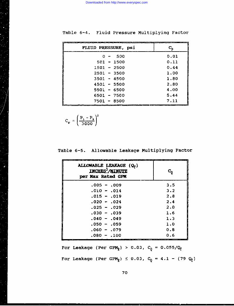
Table 6-4. Fluid Pressure Multiplying Factor

FLUID PRESSURE, psi CP

0 - 500 0.01

501 - 1500 0.11

1501 - 2500 0.44

2501 - 3500 1.00

3501 - 4500 1.80

4501 - 5500 2.80

5501 - 6500 4.006501 - 7500 5.44

7501 - 8500 7.11

3000

Table 6-5. Allowable Leakage Multiplying Factor

ALLOWABLE LEAKAGE (Qf)T 3_/jimmCQ

per Max Rated GPM

.005 - .009 3.5

.010 - .014 3.2

.015 - .019 2.8

.020 - .024 2.4

.025 - .029 2.0

.030 - .039 1.6

.040 - .049 1.3

.050 - .059 1.0

.060 - .079 0.8

.080 - .100 0.6

For Leakage (Per GPMR) > 0.03, CQ = O.055/Qf

"For Leakage (Per GPMR) • 0.03, CQ = 4.1 - (79 Qf)

70


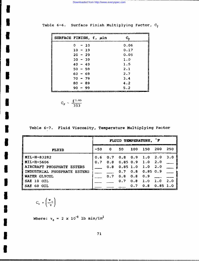
U Table 6-6. Surface Finish Multiplying Factor, CF

SURFACE FINISH, f, gin CF

0 - 10 0.0610 - 19 0.1720 - 29 0.05

30 - 39 1.040 - 49 1.550 - 59 2.1

3 60 - 69 2.770 - 79 3.480 - 89 4.2

3 90 - 99 5.2

3 CF f 1.65353a

3 Table 6-7. Fluid Viscosity, Temperature Multiplying Factor

FLUID TEMPERATURE, "F

FLUID -50 0 50 100 150 200 250

I MIL-H-83282 0.6 0.7 0.8 0.9 1.0 2.0 3.0MIL-H-5606 0.7 0.8 0.85 0.9 1.0 2.0AMAIRCRAFT PHOSPHATE ESTERS 0.8 0.85 1.0 1.0 2.0

INDUSTRIAL PHOSPHATE ESTERS 0.7 0.8 0.85 0.9WATER GLYCOL 0.7 0.8 0.8 0.9SAE 10 OIL 0.7 0.8 1.0 1.0 2.0

SAE 60 OIL 0.7 0.8 0.85 1.0

IiCIIWhere: v= 2 x 10-8 lb min/in2

* 71

I


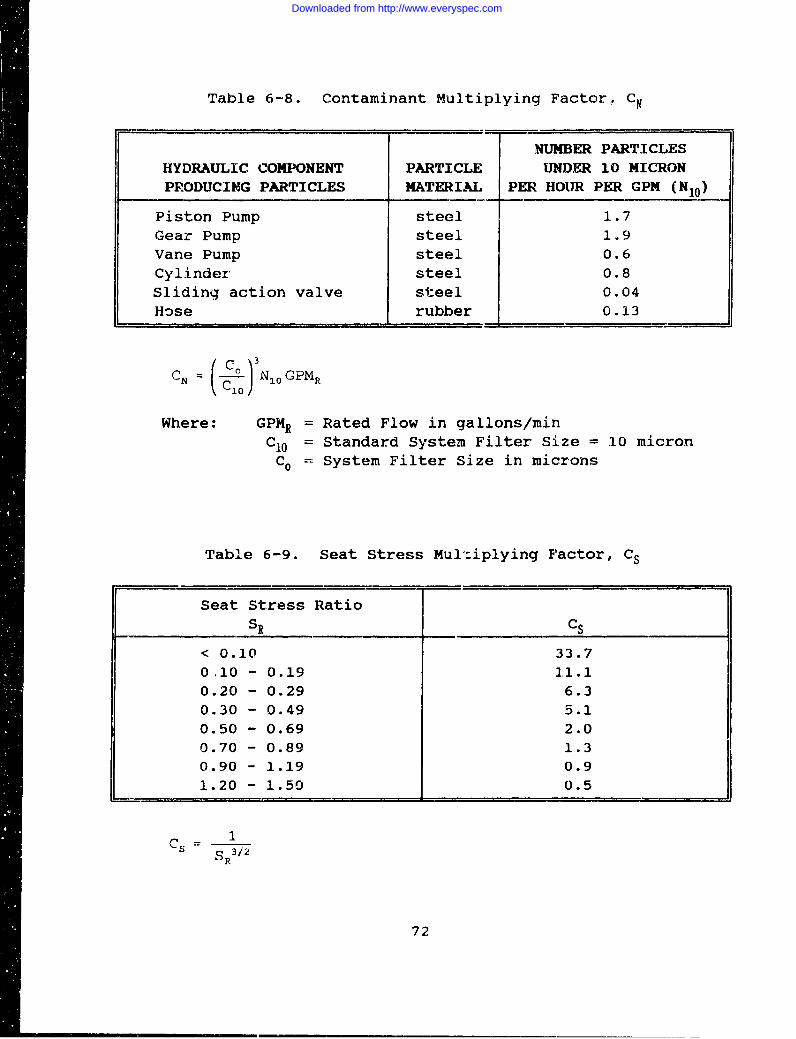
Table 6-8. Contaminant Multiplying Factor, C.

NUMBER PARTICLESHYDRAULIC COMPONENT PARTICLE UNDER 10 MICRONPRODUCING PARTICLES MATERIAL PER HOUR PER GPM (N_10 )

Piston Pump steel 1.7Gear Pump steel 1.9Vane Pump steel 0.6Cylinder steel 0.8Sliding action valve steel 0.04Hose rubber 0.13

CN = ( 3 N10 GPMR

Where: GPMR = Rated Flow in gallons/minCI0 = Standard System Filter Size = 10 micron

Co = System Filter Size in microns

Table 6-9. Seat Stress Mul:iplying Factor, Cs

Seat Stress RatioS_ Cs

< 0.10 33.701i0 - 0.19 1.1.1

0.20 - 0.29 6.30.30 - 0.49 5.1

0.50 - 0.69 2.0

0.70 - 0.89 1.3

0.90 - 1.19 0.9

1.20 - 1.50 0.5

CS= IS 3/2

72


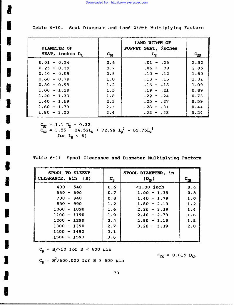
I

3 Table 6-10. Seat Diameter and Land Width Multiplying Factors

LAND WIDTH OF

DIAMETER OF POPPET SEAT, inches5 SEAT, inches DS C DT Lv Csw

0.01 - 0.24 0.6 .01 - .05 2.520.25 - 0.39 0.7 .06 - .09 2.050.40 - 0.59 0.8 .10 - .12 1.600.60 - 0.79 1.0 .13 - .15 1.31

0.80 - 0.99 1.2 .16 - .18 1.09

1.00 - 1.19 1.5 .19 - .21 0.891.20 - 1.39 1.8 .22 - .24 0.731.40 - 1.59 2.1 .25 - .27 0.59

1.60 - 1.79 2.3 .28 - .31 0.441.80 - 2.00 2.4 .32 - .38 0.24

CDT = 1.1 DS + 0. 3 2 2 3S= 3.55 - 24 .52L6 + 72 .99 LW 85 75

I~ for L. < 6)

UTable 6-11 Spool Clearance and Diameter Multiplying Factors

I -

SPOOL TO SLEEVE SPOOL DIAMETER, in1 CLEURANCE, pin (B) C B (DSP) CS

400 - 540 0.6 <1.00 inch 0.6550 - 690 0.7 1.00 - 1.39 0.8

700 - 840 0.8 1.40 - 1.79 1.0850 - 990 1.2 1.80 - 2.19 1.2

1000 - 1090 1.6 2.20 - 2.39 1.4

1100 - 1190 1.9 2.40 - 2.79 1.61200 - 1290 2.3 2.80 - 3.19 1.8

1300 - 1390 2.7 3.20 - 3.39 2.0

1400 - 1490 3.11500 - 1590 3.6I - -|

CB = B/750 for B < 600 pin-- C• = 0.615 D

CB = B2/600,000 for B g! 600 pin

*- 73

I


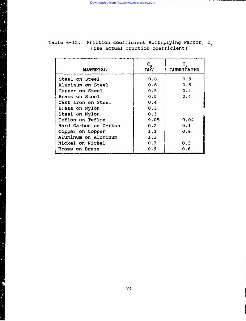
Table 6-1.2. Friction Coefficient Multiplying Factor, Cy(Use actual friction coefficient)

Cu C

MATERIAL DRY LUBRICATED

Steel on Steel 0.8 0.5Aluminum on Steel 0.6 0.5Copper on Steel 0.5 0.4Brass on Steel 0.5 0.4Cast Iron on Steel 0.4Bi'ass on Nylon 0.3Steel on Nylon 0.3Teflon on Teflon 0.05 0.04Hard Carbon on Carbon 0.2 0.1Copper on Copper 1.3 0.8Aluminum on Aluminum 1.1Nickel on Nickel 0.7 0.3Brass on Brass 0.9 0.6

74


f ~CHAP'TER 7

BEARINGS

77.1 1MYRODUCTIONBearings are among the few compcnents that are designed for a

finite life . Bearing life is generally expressed as a B10 life,which is the number of hours at a given load that 90 percent of aset of apparently identical bearings will complete or exceed.There are a number of other factors that can be applied to the B Olife so that it more accurately correlates with the intendedoperating environment. These factlrs include the use of newer highperformarce materials and manufacturing processing techniques, and

* the application of the bearing including actual lubrication filmthickness, misalignment, velocity, load stresses and subjection tocontaminants.

There are many different types of bearings in use making itextremely difficult to establish base failure rates for bearingsbased on field performance data. Bearing analysis is also

I extremely difficult due to the large number of engineeringparameters associated with bearing design. The procedures forU estimating bearing reliability presented in this chapter utilizethe manufacturer's published B,0 life with multiplying factors torelate the B10 value to intended operating conditions. An outlineI •of the basic types of bearings to be discussed is shown in Figure7.1.

I l 7.1.1 Bearing Type

bLl lBering - Ball bearings are generally used where there isU •likely to be excessive uisalignm4nt or shaft deflection. They arealso used, especially in duplex arrangements, where accurate axialpositioning is required in the presence of thrust load, such aswith bevel gear shafts. Ball bearings are not as common in themain drive train of more recent designs because of advancementsmade with tapered roller bearings. Ball bearings are, however,often used on lightly loaded accessory shafts. Higher bearing lifeis easily acnieved in these applications due to the very small).oads and installation is simplified, since a ball bearing isnons-parable and requires no special setup procedures.

* I75

I


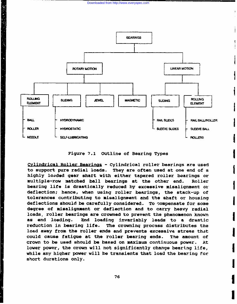
BEARUN 7 J

ROTAR MOTON LNEAR MOTION

{-o I

ELEMENT LM

NEEDLL - HLW)ROO1AMIC RAIL SUDES - RAIL BALLROLLER

ROLLER - HYDROSTATIC RSOEVE SLDS SLEEVE SALL

-NEEDE - SELF-LUBRICATING -ROLLERS

Figure 7.1 Outline of Bearing Types ICylindrical Railer Bearins, - Cylindrical roller bearings are usedto support pure radial loads. They are often used at one end of a Ihighly loaded gear shaft with either tapered roller bearings ormultiple-row matched ball bearings at the other end. Rollerbearing life is drastically reduced by excessive misalignment or Ideflection; hence, when using roller bearings, the stack-up oftolerances contributing to misalignment and the shaft or housingdeflections should be carefully considered. To compensate for some Idegree of misalignment or deflection and to carry heavy radialloads, roller bearings are crowned to prevent the phenomenon knownas end loading. End loading invariably leads to a drasticreduction in bearing life. The crowninq procsss distributes theload away from the roller ends and prevents excessive stress thatcould cause fatigue at the roller bearing ends. The amount ofcrown to be used should be based on maximum continuous power. Atlower power, the crown will not significantly change bearing life,while any higher power will be transients that load the bearing forshort durations only.

76


.. Tapered zoller bearinqs are being used.ncreasin~n'[y in modern drive systems, si.nc& they can react to both

thrust awO radial loads and can offer the vreatest load-Carryingcapacity in the smallest possible envelope. Although early taperedroller bharings were speed limited, these restrictions bave beenremoved by ut'ilizinq bearLngs with special lubrication features.SHowever, on very hiqh-speed shafts, the use of tapered rollerbearings may be precluded due to their inability to operate forrequired time intervals under survivability (oil-off) conditions.Tapered roller bearings, unlike single-row ball and cylindricalroller bearings, require spacers or shims to give these bearingsthe proper amount of preload or end play for proper operation.Usually it is desirable to have a light preload although a smallamount of end play is often acceptable. As with internalclearance, extremes in end play or preload should be scrupulouslyavoided.

- Although sleeve bearings are relativelyinexpensive, -they can cause costly equipment shutdowns if notproperly integrated into the design. Short bearing life can becaused by misalignment, a berit shaft, a rotating part rubbing on astationary part, a rotor out of balance causing vibration,3 excessive thrust caused by mechanical failure of other parts,excessive temperature caused by lack of lubrication, dirt or othercontaminant and corrosion from water in the bearing housing. Theseproblems can be classified in the following failure modes: fatigue,wiping, overheating, corrosion, and wear. Descriptions of thesemodes are as follows:I Fatigue occurs due to cyclic loads normal to the bearingsurface. Wiping occurs from surface to surface contact due to lossof sufficient lubrication film thickness. This malfunction canI occur from under-rotation or from system fluid losses. Overheatingis indicated by babbit cracking or surface discoloration.Corrosion is frequently caused by the chemical reaction between the

[] acids in the lubricants and the base metals in the babbit. Leadbased babbits tend to show a higher rate of corrosion failures.

Severe performance requirements may affect the reliability ofthe bearings if there is a path of heat conduction from the machineor any friction creating components within it to the bearings (for3 example, brakes or clutches). This condition may cause a decreasein the bearing lubricant's operating viscosity and, consequently,a reduction in bearing life. A lubricant with a higher temperatureI rating should prevent leakage or excessive wear.

77


7.1.2 Design Considerations

IlitrMnl Clearang - Internal clearance is an importantconsideration in the design of ball and roller bearings, sinceimproperly mounted internal clearance can drastically shorten thelife of a bearing. Too little internal clearance limits the amountof misalignment that can be tolerated and can lead to heavilypreloaded bearings, particularly at low temperatures. Excessiveinternal clearance will cause the load to be carried by too fewrolling elements. The best practice is to ensure that under allconditions there will be a small positive internal clearance.Usually, the most significant factors to consider when determiningmounted internal clearance of the bearing are the reduction cfinternal clearance due to shaft or housing fits and the effect oftemperature on the housing/outer race interface diameters.

Bearing Race Creep - The creeping or spinning of bearing innerraces on gearshafts is a fairly common, although not usuallyserious, problem in most drive systems. Lundberg and Palmgrendeveloped fairly simple parametric calculations for the minimum fitto prevent creep with solid shafts, but there has been little ifanything published on minimum press fits for hollow shafts, suchtypes as used in helicopter drive systems. Since an accuratemathematical solution to such a problem would be extremelydifficult, the best approach at this time seems to be a reliance onpast experience. Sometimes it may not be possible to achieve thenecessary press fit to prevent creep without introducingexcessively high hoop stress in the bearing race. A commonpractice in this case is to use separate antirotation devices witha slotted bearing race. Although this practice is fairly effectivewith stationary races, it is seldom effective with rotating races.

Bearing Material - By far the greatest advance in bearingtechnology has been the development of extremely clean bearingsteels resulting from vacuum-melt processing. Vacuum-melt 52100bearings, for example, offer one and one-half to two times the lifeof vacuum-degassed 52100 bearings. Bearings of such advancedmaterials as M-50 steel can offer even further improvement. Justbecause these materials are available, however, does not mean thatall bearings have to be made of vacuum-melt material. Depending onthe bearing, vacuum-melt bearings can be from 2 to 5 times morecostly than vacuum-degassed bearings, as well as requiring longerlead times to procure. Hence, bearings for high-speed primary

76


I

UI power train applications should be fabricated of M-50 (or in thecase of tapered roller bearings, carburized CVM steel) for the sake

I of improved survivability following loss of lubrication. All otherbearings should be fabricated of vacuum-degassed material unlessthere is a problem with low life, in which case the more expensivevacuum-melt materials should be used.

Inspection Requirement - Proper inspection of bearings cansignificantly reduce their mortality rate. Besides the obviousdimensional inspection requirements, two additional inspectionsshould be specified for all high performance drive system bearings:I Magnetic particle

. Nital etchMagnetic particle inspection can detect the presence of

relatively large surface or near-surface anomalies, such asinclusions, which are often the cause of bearing spalls. Nitaletch inspection can detect the presence of grinding burns, whichlocally change the hardness of the material and cause prematurebearing failure.

I Bearin-1 stallation/emoval - The installation of bearings shouldbe carefully considered during design not only to prevent assemblyerrors, but also to permit easy removal of the bearing withoutdamaging it. Lead chamfers should be provided at all bearingjournals to facilitate installation. When specifying the breakouton the bearing corners, the shaft drawing should be checked toensure that the maximum radius at the shaft shoulder will becleared by the bearing. The height of the shaft shoulder should,if possible, be consistent with that recommended by bearingmanufacturers. Where necessary, flats should be machined on theshaft shoulder so that a bearing puller can remove the bearing bycontacting the inner race. Many bearings have been damaged in thepast where the bearing puller could grab only the cage or rollersof the bearing. Where duplex bearings are used, the bearingsshould be marked so that the installer can readily determine theproper way for the bearings to be installed. Incorrectly installedduplex bearings will not properly react to the design loads. Allbearings that can be separated should have the serial numberclearly shown on all of the separable components. This willprevent the inadvertent mixing of components. Every assemblydrawing that contains bearings should clearly explain in thedrawing notes how the bearing should be installed. It isimperative that the mechanics building up this assembly have this

* 79

I


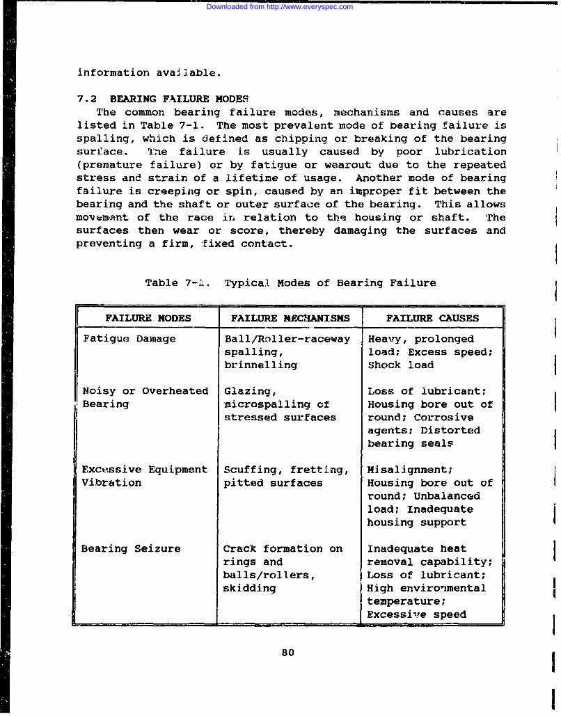
information available.

7.2 BEARING FAILURE MODESThe common bearing failure modes, mechanisms and causes are

listed in Table 7-1. The most prevalent mode of bearing failure isspalling, which is defined as chipping or breaking of the bearingsurface. The failure is usually caused by poor lubrication(premature failure) or by fatigue or wearout due to the repeatedstress and strain of a lifetime of usage. Another mode of bearingfailure is creeping or spin, caused by an improper fit between thebearing and the shaft or outer surface of the bearing. This allowsmovempnt of the race in relation to the housing or shaft. Thesurfaces then wear or score, thereby damaging the surfaces andpreventing a firm, fixed contact.

Table 7-1. Typical Modes of Bearing Failure

FAILURE MODES FAILURE MECHANISMS FAILURE CAUSES

Fatigue Damage Ball/Roller-raceway Heavy, prolongedspalling, load; Excess speed;brinnelling Shock load

Noisy or Overheated Glazing, Loss of lubricant;Bearing microspalling of Housing bore out of

stressed surfaces round; Corrosiveagents; Distortedbearing seals

Excessive Equipment Scuffing, fretting, MJsalignment;Vibration pitted surfaces Housing bore out of

round; Unbalancedload; Inadequatehousing support

Bearing Seizure Crack formation on Inadequate heatrings and removal capability;balls/rollers, Loss of lubricant;skidding High environmental

temperature;Excessive speed

80


I

I Roller and tapered bearings have an additional failure modedefined as hard lines or scuffing of the bearing surfaces. Thisfailure mode is usually caused by bearing exposure to an excessiveload for an extensive period of time. The surfaces of the movingparts are scored or scratched, increasing the roughness of the5 surfaces, setting up stress concentrations and increasingfriction. The scoring also interferes with the normal lubricantfilm and increases the metal-to-metal contact during use.

7.3 BEARING FAILURE RATE PREDICTIONBearing life is usually calculated using the Lundberg-Palmgren

method (Ref. 53). This method is a statistical tecanique based onthe sub-surface initiation of fatigue cracks through hardenedair-melt bearing material. Most mechanical systems are notutilized precisely as the bearing manufacturer envisioned;therefore, some adjustment factors must be used to approximate thefailure rate of the bearings under specific conditions.

Experience has shown that the service life of a bearing isusually limited by either excessive wear or faigue. Excessive3 wear occurs when the bearings are improperly installed or exposedto hostile operating environments. Inadequate lubrication,misalignment, contamination, shock, vibration, or extremetemperature all cause bearings to wear out prior to their estimateddesign life. In contrast, a 'Aearing can be expected to performadequately for the duratir)n )f its rated life, given proper

I operating conditions, until farI lure occurs due 'to fatigue.All. bearings ultimately fai due to fatigue because the load

carrying balls, raceways, rollers, etc. are subjected to cyclicalScontact stresses. Under laboratory conditions the fatigue

characteristics of bearings can be quantified in terms of stressmagnitude and number of stress cycles, which in turn relates to thebearing load and number of revolutions. A heavily loaded bearing,for example, has a much shorter fatigue life than a lightly loadedone when both are operated at the same low speed. Conversely, abearing operated under a ligkt load and low speed provides aservice life several times greater than the rated life. In this5 latter case service will generally be terminated by wear.

Attempting to estimate the fatigue life of an individual bearingis not very practical because of the large number of designparameters to consider in relation to the sensitivit, of theoperating environment. Instead, statistical methods are used torate bearings based on the results of large groups of the same Lypeof bearing tested to failure under controlled laboratory conditions

* 81


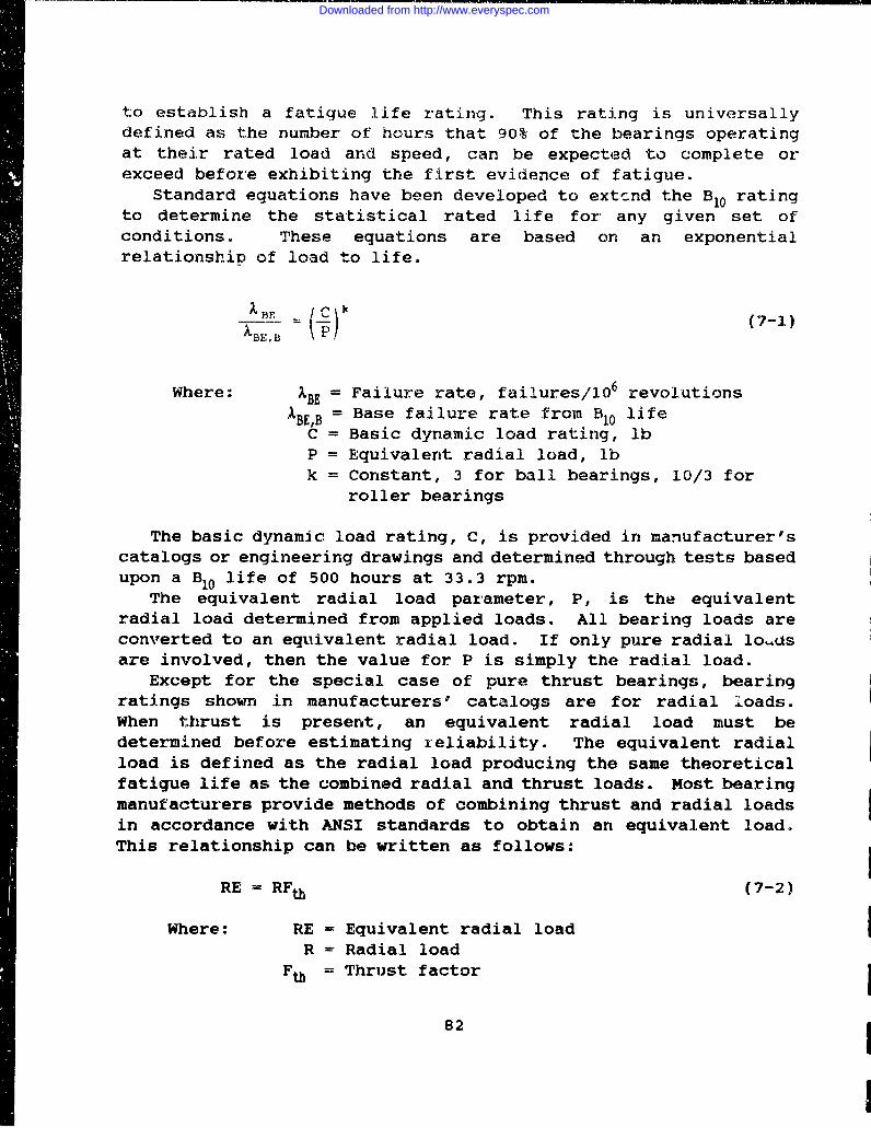
to establish a fatigue life rating. This rating is universallydefined as the number of hours that 90% of the bearings operatingat their rated load and speed, can be expected to complete orexceed before exhibiting the first evidence of fatigue.

Standard equations have been developed to extcnd the B 0 ratingto determine the statistical rated life for any given set ofconditions. These equations are based on an exponentialrelationship of load to life.

1 .3F - (7--1)

Where: XBE = Failure rate, failures/106 revolutionsxBEB Base failure rate from B10 life

C = Basic dynamic load rating, lbP = Equivalent radial load, lbk = Constant, 3 for ball bearings, 10/3 for

roller bearings

The basic dynamic load rating, C, is provided in manufacturer'scatalogs or engineering drawings and determined through tests basedupon a B10 life of 500 hours at 33.3 rpm.

The equivalent radial load parameter, P, is the equivalentradial load determined from applied loads. All bearing loads areconverted to an equivalent radial load. If only pure radial lo"Isare involved, then the value for P is simply the radial load.

Except for the special case of pure thrust bearings, bearingratings shown in manufacturers' catalogs are for radial loads.When thrust is present, an equivalent radial load must bedetermined before estimating reliability. The equivalent radialload is defined as the radial load producing the same theoreticalfatigue life as the combined radial and thrust loads. Most bearingmanufacturers provide methods of combining thrust and radial loadsin accordance with ANSI standards to obtain an equivalent load.This relationship can be written as follows:

RE = RF• (7-2)

Where: RE = Equivalent radial loadR = Radial load

Ft = Thrust factor

82


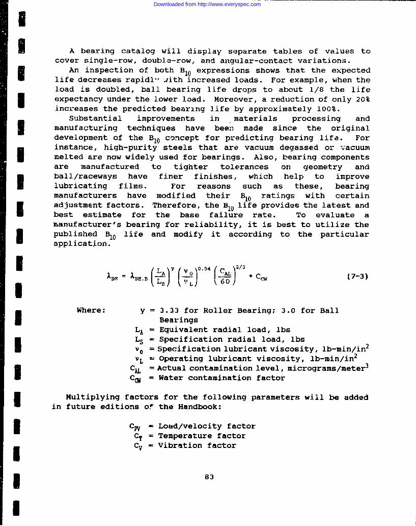
U lA bearing catalog will display separate tables of values tocover single-row, double-row, and angular-contact variations.

An inspection of both B10 expressions shows that the expectedlife decreases rapidl" with increased loads. For example, when theload is doubled, ball bearing life drops to about 1/8 the lifeexpectancy under the lower load. Moreover, a reduction of only 20%increases the predicted bearing life by approximately 100%.

Substantial improvements in materials processing and3 manufacturing techniques have been made since the originaldevelopment of the B10 concept for predicting bearing life. Forinstance, high-purity steels that are vacuum degassed or vacuumI melted are now widely used for bearings. Also, bearing componentsare manufactured to tighter tolerances on geometry andball./raceways have finer finishes, which help to improveU lubricating films. For reasons such as these, bearingmanufacturers have modified their B10 ratings with certainadjustment factors. Therefore, the B10 life provides the latest andbest estimate for the base failure rate. To evaluate amanufacturer's bearing for reliability, it is best to utilize thepublished B10 life and modify it according to the particularapplication.

I ~~~L )B BE()Y (Lo) 0 , 5 4 ( CL)2/3*(-)U AB IB J Ls) t •L) 60 C C W (7-3)

Where: y = 3.33 for Roller Bearing; 3.0 for BallI Bearings

LA = Equivalent radial load, lbsLS = Specification radial load, lbsV0 = Specification lubricant viscosity, lb-min/in2

vL -Operating lubricant viscosity, lb-min/in2

ICk = Actual contamination level, micrograms/meter 3

CC = Water contamination factor

Multiplying factors for the following parameters will be addedin future editions of the Handbook:

Ip = Load/velocity factorCT = Temperature factorCV = Vibration factor

* I83

I


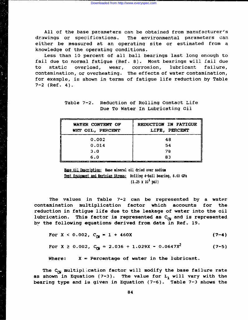
All of the base parameters can be obtained from manufacturer'sdrawings or specifications. The environmental parameters caneither be measured at an operatinq site or estimated from aknowledge of the operating conditions.

Less than 10 percent of all ball bearings last long enough tofail due to normal fatigue (Ref. 8). Most bearings will fail dueto static overload, wear, corrosion, lubricant failure,contamination, or overheating. The effects of water contamination,for example, is shown in terms of fatigue life reduction by Table7-2 (Ref. 4).

Table 7-2. Reduction of Rolling Contact LifeDue To Water In Lubricating Oil

WATER CONTENT OF REDUCTION IN FATIGUEWET OIL, PERCENT LIFE, PERCENT

0.002 480.014 543.0 786.0 83

Base Oil Desc•iRtion: Base mineral oil dried over sodiumTest Ewipmnt and Hertzian Stress: Rolling 4-ball bearing, 8.60 (Wa

(1.25 x 104 psi)

The values in Table 7-2 can be represented by a watercontamination multiplication factor which accounts for thereduction in fatigue life due to the leakage of water into the oillubrication. This factor is represented as C• and is representedby the following equations derived from data in Ref. 19.

For X < 0.002, C• = 1 + 460X (7-4)

For X 2 0.002, CC = 2.036 + 1.029X - 0.0647X2 (7-5)

Where: X = Percentage of water in the lubricant.

The CC multiplication factor will modify the base failure rateas shown in Equation (7-3). The value for LA will vary with thebearing type and is given in Equation (7-6). Table 7-3 shows the

84


I equations that represent the load capacity for the various types ofbail and roller bearings.

Table 7-4 gives values for fc used to determine LA in Equation(7-6) for the various types of bearing configurations. The valueof fc is used in the Ls equation(s) of Table 7-3. This is the valuein the denominator of the bearing load factor in Equation 7-4. LAis determined using the following equation:

3 LA = XFr + YFa (7-6)

I where X and Y are listed in Table 7-5 for the various bearing typesand designs. The value for Ls is obtained from Tables 7-3 and 7-4and then used in Equation (7-3) along with the value from Equation

I (7-6) to find the expected bearing reliability.

iI

I

IiU

II


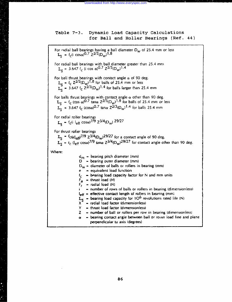
Table 7-3. Dynamic Load Capacity Calculationsfor Ball and Roller Bearings (Ref. 44)

For radial ball bearings having a ball diameter Dw of 25.4 mm or lessLS - fc(i cosa)0 .7 Z2 /3 (Dw)1 .8

For radial ball bearings with ball diameter greater than 25.4 mmLS - 3.647 fc (i Cos a)0 .7 Z2/ 3 (Dw)1.4

For ball thrust bearings with contact angle a of 90 deg.

LS - fc Z2/ 3 (Dw)T1 8 for balls of 25.4 mm or less

LS - 3.647 fc Z2/ 3 (Dw)1"4 for balls larger than 25.4 mm

For balls thrust bearings with contact angle ce other than 90 deg.Ls - fc (cos a)0 .7 tanci Z2/ 3 (Dw) 1 "8 for balls of 25.4 mm or less

L S - 3.647 fc (cosax) 0 "7 tance Z2/ 3 (Dw) 1 .4 for balls 25.4 mm

For radial roller bearings

LS - fc(i leff cosa) 7 /9 Z3 /4 (Dw) 29/27

For thrust rolier bearings

LS - fc6(leff)7/ 9 Z3 /4 (Dw)2 9 /2 7 for a contact angle of 90 deg.

LS - tc (leff cosa) 7 /9 tana Z3 /4 (Dw)2 9/ 2 7 for contact angle other than 90 deg.

Where:dm - bearing pitch diameter (mm)D - bearing outer diameter (mm)Dw - diameter of balls or rollers in bearing (mm)e - equivalent load functionfc - bearing load capacity factor for N and mm unitsFa - thrust load (N)Fr - radial load (N)i - number of rows of balls or rollers in bearing (dimensionless)Ijff - effective contact length of rollers in bearing (mm)Ls - bearing load capacity for 106 revolutions rated life (N)X - radial load factor (dimensionless)Y - thrust load factor (dimensionless)Z - number of ball or rollers per row in bearing (dimensionless)a - bearing contact angle between ball or roiter load line and plane

perpendicular to axis (degrees)

86


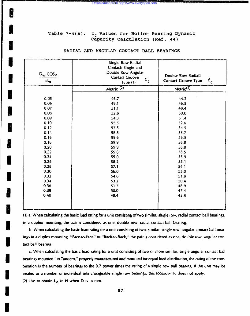
Table 7-4(a). fc Values for Roller Bearing DynamicCapacity Calculation (Ref. 44)

HRADIAL AND ANGULAR CONTACT BALL BEARINGS

Single Row RadialContact: Single and

i Dw Cosa Double Row Angular Double Row RadiailD Contact Groove Dul o ail

dmType (1) C Contact Groove Type fc

Metric (2) Metric(2 )

0.05 46.7 44.20.06 49.1 46.5

0,07 511. 48.40.08 52.8 50.00.09 54.3 51.4

I 0.10 55.5 52.60.12 57.5 54.50.14 58.8 55.70.16 59.6 56.50.18 .59.9 56.80.20 59.9 56.80.22 59.6 56.50.24 59.0 55.90.26 58.2 55.10.28 57.1 54.10.30 56.0 53.00.32 54.6 51.80.34 53.2 50.40.36 51.7 48.9I 0.38 50.0 47.40.40 48.4 45.8

I-'(1) a. When calculating the basic load rating for a unit consisting of two similar, single row, radial contact ball bearings,

in a duplex mounting, the pair is considered as one, double row, radial contact ball bearing.

b. When calculating the basic load rating for a unit consisting of two, similar, single row, angular contact ball bear-

ings in a duplex mounting. "Face-to-Face" or "Back-to-Back," the pair is considered as one, double row, angular con-

tact ball bearing.

c. When calculating the basic load rating for a unit consisting of two or more similar, single angular contact ball

bearings mounted "in Tandem," properly manufactured and moui ýted for equal load distribution, the rating of the com-

bination is the number of bearings to the 0.7 power times the rating of a single row ball bearing. If the unit may be

treated as a number of individual interchangeable single row bearings, this footnote 1c does not apply

(2) Use to obtain LA in N when D is in mm.

3 87


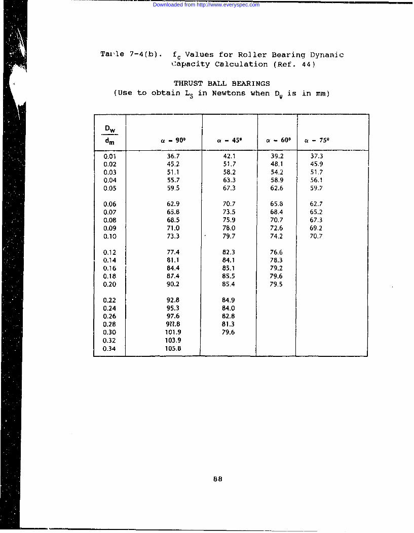
Taile 7-4(b). fc Values for Roller Bearing DynamicCapacity Calculation (Ref. 44)

THRUST BALL BEARINGS(Use to obtain Ls in Newtons when Dw is in mm)

Dw

dm - 9 09 - 450 - 60 0 - 750

0.01 36.7 42.1 39.2 37.30.02 45.2 51.7 48.1 45.90.03 51.1 58.2 54.2 51.70.04 55.7 63.3 58.9 56.10.05 59.5 67.3 62.6 59.7

0.06 62.9 70.7 65.8 62.70.07 65.8 73.5 68.4 65.20.08 68.5 75.9 70.7 67.30.09 71.0 78.0 72.6 69.20.10 73.3 79.7 74.2 70.7

0.12 77.4 82.3 76.60.14 81.1 84.1 78.30.16 84.4 85.1 79.20.18 87.4 85.5 79.60.20 90.2 85.4 79.5

0.22 92.8 84.90.24 95.3 84.00.26 97.6 82.80.28 9??.8 81.30.30 101.9 79.60.32 103.90.34 105.8

8

88


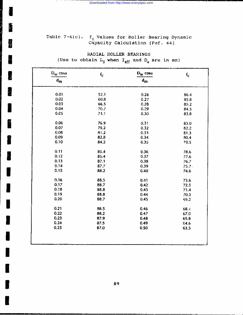
II

TabIc. 7-4(c). E. Values for Roller Bearing DynamicCapacity Calculation (Pef. 44)

RADIAL ROLLER BEARINGS(Use to obtain L, when Ieff and Dw are in mm)

Dw cosa fc Dw Cosa fc

dm dm

I 0.01 52.1 0.26 86.40.02 60.8 0.27 85.80.03 66.5 0.28 85.20.04 70.7 0.29 84.50.05 74.1 0.30 83.8

0.06 76.9 0.31 83.00.07 79.2 0.32 82.20.08 81.2 0.33 81.30.09 82.8 0.34 80.40.10 84.2 0.35 79.5

0,11 85.4 0.36 78.60.12 86.4 0.37 77.60.13 87.1 0.38 76.70.14 87.7 0.39 75.7.0.15 88.2 0.40 74.6

0.16 88.5 0.41 73.60.17 88.7 0.42 72.50.18 88.8 0.43 71.40.19 88,8 0.44 70.30.20 88.7 0.45 69.2

0.21 88.5 0.46 68. 10.22 88.2 0.47 67.00.23 87.9 0.48 65.80.24 87.5 0.49 f.4.60.25 87.0 0.50 63.5

9II

I


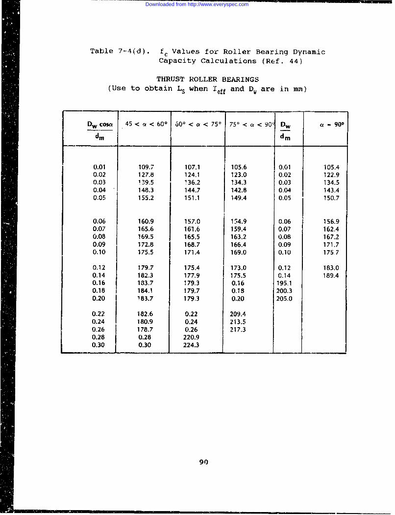
Table 7-4(d). fc Values for Roller Bearing DynamicCapacity Calculations (Ref. 44)

THRUST ROLLER BEARINGS(Use to obtain Ls when Ieff and Dw are in mm)

Dw cosa 4 5 < a < 600 60 0 < a < 750 750 < a < 90': Dw c - 900

dm dm

0.01 109.7 107.1 105.6 0.01 105.40.02 127.8 124.1 123.0 0.02 122.90.03 139.5 136.2 134.3 0.03 134.50.04 148.3 144.7 142.8 0.04 143.40.05 155.2 151.1 149.4 0.05 150.7

0.06 160.9 157.0 154.9 0.06 156.90.07 165.6 161.6 159.4 0.07 162.40.08 169.5 165.5 163.2 0.08 167.20.09 172.8 168.7 166.4 0.09 171.70.10 175.5 171.4 169.0 0.10 175.7

0.12 179.7 175.4 173.0 0.12 183.00.14 182.3 177.9 175.5 0.14 189.40.16 133.7 179.3 0.16 195.10.18 1 184.1 179.7 0.18 200.30.20 '83.7 179.3 0.20 205.0

0.22 182.6 0.22 209.40.24 180.9 0.24 213.50.26 178.7 0.26 217.30.28 0.28 220.90.30 0.30 224.3

90


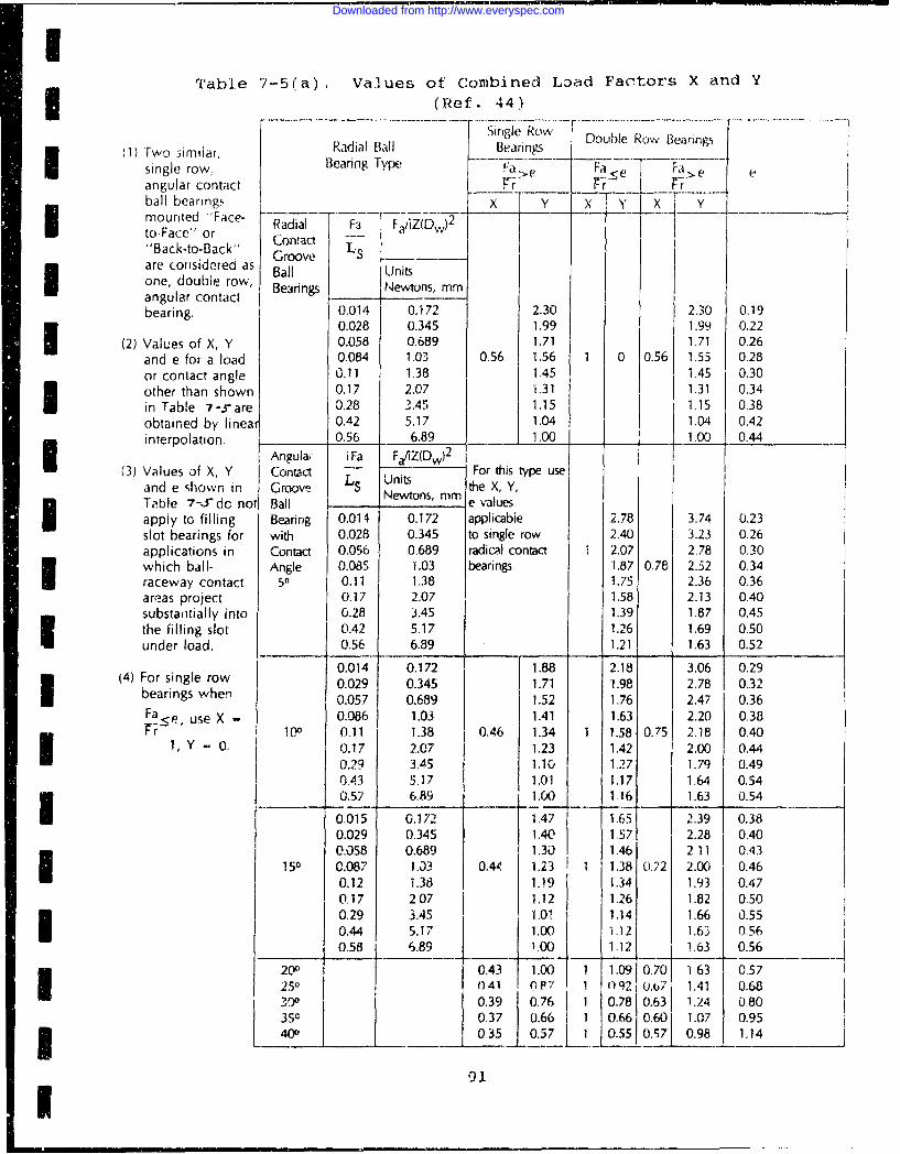
ITable 7-5(a). Values of Combined Load Factors X and Y

(Ref. 44.)

Single Row Double Row Bearings1 Two 3imdiar, Radial Ball Bearings i

single row, Bearing Type Fa >e Fa e F.> e

angular contact FFT Frball bearings X Y .Y • Ymounted "Face- ad -F FiZ(to-Face" or Contact W"Back-to-Back" Groove LSare comsidered as Ball Unitsone, double row-, Bearings Newtons, u mangular contactbearing. 0.014 0.172 2.30 2.30 0.19

0.028 0.345 1.99 1.99 0.22(2) Values of X, Y 0.058 0.689 1.71 1.71 0.26

and e for a load 0.084 1.03 0.56 1.56 1 0 0.56 1.55 0.28or contact angle 0.11 1.38 1.45 1.45 0.30other than shown 0.17 2.07 i.31 1.31 0.34in Table 7-J are 0.28 3.45 1.15 1.15 0.38obtained by linea 0.42 5.17 1.04 1.04 0.42interpolation. r_ _ 0.56 6.89 1.00 1.00 0.44

Angula& i Fa Fa/iZ(Dw)2

(3) Values of X, Y Contact - For this type use

and e shown in Groove LS Units the X, Y,Table 7-Jcdo not Ball - Newtons, mm e valuesapply to filling Bearing 0.0114 0.172 applicabie 2.78 3.74 0.23slot bearings for with 0.028 0.345 to single row 2.40 3.23 0.26applications in Contact 0.056 0.689 radicAl contact 1 2.07 2.78 0.30which ball- Angle 0.085 1.03 bearings 1.87 0.78 2.52 0.34raceway contact 50 0.11 1.38 1.75 2.36 0.36areas project 0.17 2.07 1.58 2.13 0.40substantially into 0.28 3.45 1.39 1.87 0.45the filling slot 0.42 5.17 1.26 1.69 0.50under load. 0.56 6.89 1.21 1.63 0.52

0.014 0.172 1.88 2.18 3.06 0.29(4) For single row 0.029 0.345 1.71 1.98 2.78 0.32

bearings when 0.057 0.689 1.52 1.76 2.47 0.36Fae, use X 0.086 1.03 1.41 1.63 2.20 0.38

100 0.11 1.38 0.46 1.34 1 1.58 0.75 2.18 0.40I, Y 0,. 0.17 2.07 1.23 1.42 2.00 0.44

0.29 3.45 1,10 1.27 1.79 0.490.43 5.17 1.01 1.17 1.64 0.54o.57 6.89 1.CK) 116 1.63 0.54

0.015 0. 172 1.47 1.65 2.39 0.380.029 0.345 1.40 1 57 2.28 0.400.058 0.689 1.30 1.46 2.11 0.43

150 0.087 1.[]3 0.4- 1.23 1 1.38 0.2 2.00 0.460.12 1.38 1.19 1.34 1.93 0.470.17 207 '1.12 1.26 1.82 0.500.29 3.45 1.01 1.14 1.66 0.550.44 5.17 1.00 1.1,2 1.63 0.560.58 6.89 i.00 1.12 1.63 0.56

200 0.43 1.00 1 1.09 0.70 1 63 0.57I 2501 041 PY I ()92 0.b7 1.41 0.68

390 0.39 0.76 1 0.78 0.63 1.24 0.80350 f 0.37 0.66 1 0.66 0.6 1.07 0.95

400.35 0.57 1 0.55 0.7 0.98 1.14

91


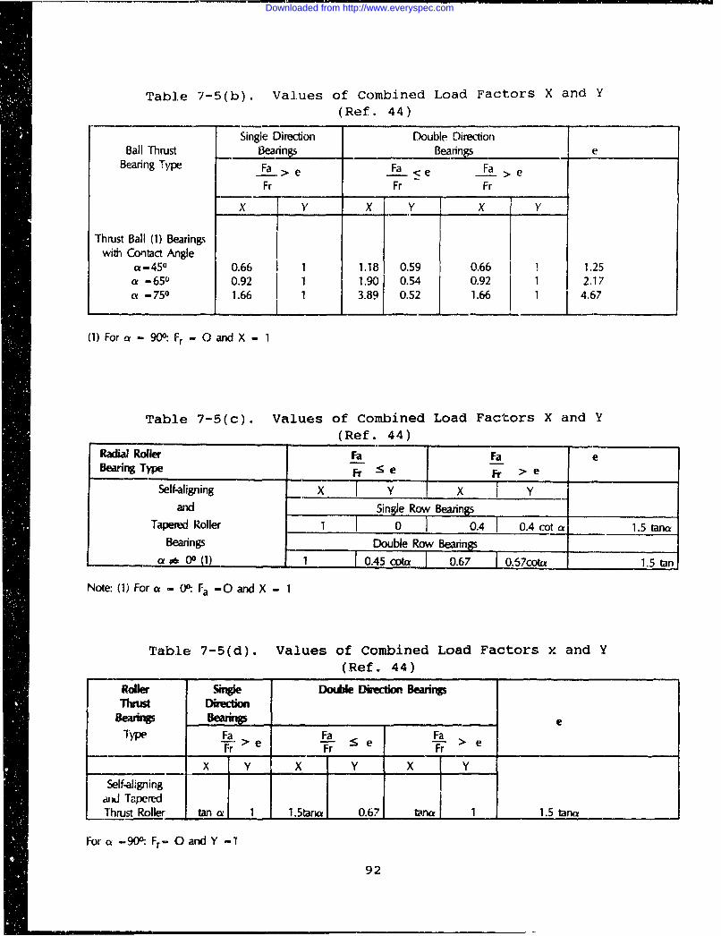
Table 7-5(b). Values of Combined Load Factors X and Y(Ref. 44)

Single Direction Double DirectionBall Thrust Bearings Bearing e

Bearing Type -La- > e Fa < e Fa > e

Fr Fr Fr

x Y X Y X Y

Thrust Ball (1) Bearingswith Contact Angle

ct-450 0.66 1 1.18 0.59 0.66 1 1.25a-650 0.92 1 1.90 0.54 0.92 1 2.17

- 750 1.66 1 3.89 0.52 1.66 1 4.67

(1) Fora - 900: Fr - 0 and X - 1

Table 7-5(c). Values of Combined Load Factors X and Y(Ref. 44)

Radial Roller Fa Fa eBearing Type Fr < e Fr > e

Self-aligning x Y X i Yand Single Row Bearings

Tapered Roller 1 0 0.4 0.4 cota 1.5 tanaBearings Double Row Bearings

a ;.& 00 (1) 1 0.45 cOpt 0.67 0.57cota 1.5 tan

Note: (1) For a - 00: Fa -O and X - 1

Table 7-5(d). Values of Combined Load Factors x and Y(Ref. 44)

Roller Sinle Double Dire•bon BearingsThrust Diretion

Beadripg B __________ eTyeFa> Fa FaIyeFa' > e fa-7 :. e fa-I > e

Fr- Fr ~eFrX Y x Y X Y

Self-aligning.u•J Tapered

Thrust Roller tan a 1 1.5tar, 0.67 _ _ 1 1.5 tan_-

For a -900: Fr- 0 and Y -1

92


II

SI CHAPTER 8

3 GEARS AND SPLINES

8.1 INTRODUCTIONThe reliability of gear or drive components is perhaps one of

the most important considerations when designing a system. Somegeneral design constraints and requirements should be given specialattention because of their potential impact on the long-termreliability of the total system. The first of these is the

I operating power spectrum. The key point with regard to this designparameter is to anticipate potential requirements for growth. Thesecond is that changing requirements may cause a configurationchange where alignments are altered. This can be critical if the

i misalignment could cause vibration that could set up stresses aridlead to fatigue failure. When a lubrication system is included,care should be taken to assure that the capacity, filter andtransferring components are adequate. If superfine filters shouldbe introduced, larger traps would be required to accommodate the3increase in particles trapped in the element. The lubricant flowshould be designed so that the particles within the system areremoved prior to reentry into the gear box area.

Noise and vibration can affect reliability, not only the drivesystem itself, but also associated components of the completesystem. Hence, every effort should be made to select a gearboxthat is as quiet and as vibration-free as possible. When selectinggear candidates, consideration should be given to helical or highcontact spur gears instead of conventional spur gears. Also, oneshould make certain that critical speeds and gear clash resonancefrequencies, which may reinforce each other, are avoided.'3 In most gearbox applications, especially in Airborne Systems,weight is usually a constraining and, in some cases, thecontrolling factor. In general, overdesign means higher3 reliability, but in weight critical systems, overdesign in one arearequires underdesign elsewhere; thereby, defeating the purpose ofthe overdesign. For example, bearing life should never besacrificed in the design because bearings are likely to be the maindrivers in the establishment of the failure rates of the gearsystem.

When a gearbox is exposed to overstress, several conditions

1 93

I


occur that greatly affect the failure rate. Bolted gear flangeswill be subject to fretting, hiqh loads will cause bevel, gears toshift patterns, making tooth breakage a likely occurrence. Spurgears develop hard lines or scuffing as loads are increased. Theuse of a gear system in a design that exceeds the specificationload should be done only after detailed analysis of the impact oneach part or component has been made.

8.2 FAILUPE MODES

8.2.1 SpradHlia ý,rSpur gears are commonly used in all types of gearing situations,

both for parallel-axis speed reduction and in coaxial planetarydesigns. In general, the reliability of drive train spur gears ii;extremely high due to present design standards. There are,however, some considerations that should be addressed because theyare frequently overlooked in spur gear design or selection forspecific purposes.

Generally, the initial design of a spur gear mesh is one ofstandard proportions and equal tooth thickness for both pinion andgear. This is, however, rarely the optimum configuration for aspur gear mesh, because this type of design does not have two verydesirable characteristics: recess action and a balanced bendingstress in pinion and gear. A recess-action gear mesh has a longaddendum pinion and short addendum gear. A recess-action mesh isquieter and smoother running than standard mesh and has a muchlower tendency to score due to better lubrication within the mesh.

Although the adva•ntage of having balanced bending stresses on apinion and gear is primarily lower weight, it does have an indirecteffect on reliability. As stated earlier, whenever there is aninefficient use of weight, reliability is compromised somewhat.For example, even a fraction of a pound wasted to non-optimizationof a 7pur gear mesh could be applied to a bearing where the lifecoulc perhaps be doubled. While overemphasis of weight reductioncan be detrimental to reliability, the carrying of excess weightcan have a far-reaching effect; therefore, a balanced gear systemmust be the goal tor efficient and reliable systems. Fortunately,it is usually a simple task io achieve rocess-action and balancedbonding stress in most spur gear designs. This is accomplished byexperimentally shifting the length of contact up the line of actiontoward the driver gear, while increasing the circular tooththickness of the pinion and decreasing that of the gear.

94


TI There are four design criteria that are used to evaluate theadequacy of spur or helical design: Bending stress, hertz orvibrational stress, flash temperature index and/or lubrication filmthickness (EHD). The first three have long been used in geardesign and methods of calculation are well documented in manyif publicaticns. EHD (Elastrohydrodynamic) film thickness is a newertechnique and has not yet beer, completely standardized. Some gearspecialists have advanced EHD film thickness as a check on scoringprobability. It is obvious that if an oil film of a greaterthickness than the contact surface asperities can be maintainedscoring will not occur, since a metal-to-metal contact must beexperienced to allow scoring to occur.

An important parameter to evaluate lubrication effectiveness isI the lubricant film thickness. The equation below is a non-dimensional expression for lubricant film thickness:

I HL = 2. 5G 4 U°' (8-1)WO.13

Where: HL = Dimensionless film thicknessG = Viscosity and material parameterU = Speed parameterW = Load parameter

Since it is often difficult to obtain these parameters directly,this expression will only be used for a qualitative evaluation.The major- impact of the formula is to establish the dependence oflubricant film thickness (H) from the various parameters. Itshould be noted that a change in lubricant viscosity and gearsystem velocity have a major impact on h, whereas a change in loadhas a weaker influence. These trends can be used when adjustment

factors are developed later in the text.N Allowable tooti stress is the subject of much uncertainty andmost gear manufacturers have a proprietary method for establishingthis criteria. Therefore, it is usually a stated parameter fromSthe manufacturer that is used. The use cf allowable stresspublished by AGMA rivll usually result in satisfactory gearperformance.

To ensure smooth operation of the gear mesh under load, it isgenerally the practice to mod).fy .he involute profile, usually withtio !-elief, to correct for the deflection of the gear, tooth underload. %he dafle'•tion can be accurately calculated, therefore, the

95

I


correct deflection profile should be used. Too little relief willresult in the gear teeth going into mesh early and going out ofnmesh late. This results in higher dynamic loads with theaccompanying stress, vibration, noise and possible non-involutecontact that can lead to hard-lines, scuffing or scoring of gearteeth. Too much tip relief lowers the contact ratio of the gearset and again can result in less than optimum performance withrespect to stress, vibration, and noise.

Crowning is generally applied to spur gears to ensure fullcontact across the face of the gear without end loading. Withinsufficient crowning, end loading will occur and result in higherthan predicted vibrational stresses. The methods used to calculatethe amount of crowning is sim-'ar to the methods used fol-calculating crowning on roller bearings.

Helix correction must be used if the bearing mountings of thespur gear are not of equal stiffness. This causes the gear to cockand concentrate the load at one end of the gear tooth. Analyticalprediction is not usually practical and strain gaging the gear rimis the better method to determine helix corrections. This processinvolves iterative grinding and testing until an equal reading isobtained acrosc the gear face. Edge break is advisable for allgear teeth, including spiral bevel and helical teeth. This willprevent chipping of the gear teeth at the corners, whichcarburization has made quite brittle.

Helical gears are usually quieter and have a greaterload-carrying capacity per inch of face than spur gears. The majordisadvantage is that a thrust load is introduced along the gearshaft, thereby requiring largcr and stronger bearings. Analysis ofhelical gears is very similar to that used for spur gears. Thestress analysis is performed using an equivalent spur tooth. AGMAstandard procedures have been developed for strength analysis ofspur and helical gears.

8.2.2 9irAJlDWY&JL_&4ruThe geometry of spiral bevel gears is considerably more complex

than the spur or helical gear; therefore spiral bevel gears areprobably the most difficult type gear to design and analyze. Thehand of spiral gears should be chosen, if possible, so that axi:.iforces tend to push both the pinion and gear out of mesh. 7if thisSi• •upossible, then the hand is chosen so the pinion is forced outof mesh. The Zace contact ratio of the mesh should be as high aspossible to ensure quiet running. The face width of the spiralbevel aear should never exceed one-third of tthe outer cone distance

96


I to prevent load concentration on the toe of the gear and possibletooth breakage.

1 8.2.3 netary GeapPlanetary gear units are used in many designs, because they3 cffer relatively large speed reduction in a compact package. The

load shared among the pinions and the face width of the planetarygear is much less than that which would be required for a singlemesh reduction. From a design point of view, it is desirable touse as many pinions as possible. It is normally desired to refrainfrom equally spaced planets meshing in unison with a sun or ringgear. The most common problem with this design is thrust washerwear. The excessive wear generally results from an inadequatesupply of lubricant to the thrust washer area. The sphericalbearing type support is generally preferred from a reliabilitypoint of view, since there are fewer parts and the thrust washerproblem is eliminated. The spherical bearings also allow thepinions to maintain alignment with the sun and ring gears despitethe deflection of the pinion posts. Despite the advantage of thisdesign, it may be impossible to provide adequate support forcantilevered pinions in high torque situations, thereby requiring

i a two-plate design.

8.2.4 IMMv9•_•ieInvolute splines are used to transfer torque between shafts and

flanges, gears and shafts, and shafts and shafts. The most cormonproblem associated with splines is wear due to fretting;particularly, with loose splines. Strict attention must be given1 to the maintenance of bearing stress below the allowable limit.Tight splines should have an adequate length pilot to react withbending loads. Lubrication is a par::icular factor in thereliability of loose splines and, if at all possible, should remainflooded with oil at all times. Crowning is usually required to

i prevent excessive wear.

8.3 GEAR RELIABILITY PREDICTIONif The previous paragraphs have provided an insight into thespecific characteristics and failure modes of the more common geartypes. Gears, fortunately, &re designed to a specification andthrough the standardization of the American Gear Manufacturer'sAssociation (AGMA), gears of various manufacturers and designs canbe compared. The best approach for the calculation of failurerates for a gear system is to use the manufacturer's specification

1 97


for each gear as the base failure rate, and adjust the failure ratefor any difference in the actual usage from that purpose for whichthe gear was designed. This gear failure rate can be expressed as:

AGE = AGEB " .C * CGL * C * • CGT ' CGV (8-2)

Where: AGE Failure Rate of Gear under specific operation,failures/million revolutions

AGEB = Base Failure of Gear specified by manufacturer,failures/million revolutions

CGS = Multiplying factor considering speed deviationwith respect to design

CGP Multiplying factor considering torque deviationwith respect to design

SC• =Multiplying factor considering misalignmentCGL = Multiplying factor considerinq lubrication

deviation with respect to designSCG= Multiplying factor considering contamination

environment-CG= Multiplying factor considering temperatureCG = Multiplying factor considering vibration and shock

IGEB can usually be obtained from the manufacturer and it willbe expressed in failures/operating hour at a specified speed, lead,lubricant, and temperature. Also, a service factor will usually beprovided to adjust the normal usage factor for certain specificconditions found in typical industries. These factors include suchthings as vibration, shock, contamination, temperature and usagerate.

CGS can be calculated by using the information provided byEquation (8-1) noting that the lubrication film thickness varieswith speed to the 0.7 power. Therefore:

SOpezating Speed)O.7 (8-3)

CG or load factor has a lubricant and a fatigue impact. Fromprevious expressions of EHD, the impact of load or torque can beexpressed as:

From Equation (8-1):

98


IChange in Expected Life - 1 _ (Lubricant Impact) (S-4)w , 13 I 0.

i Where: L = Operating LoadLD = Design Load

and the expression for torque or load on the fatigue rate of tnecomponent is:

4.561 Change in Expected Life (Fatigue Impact)

Therefore:

c o )Y.69 (8-6)

The alignment of gears, bearings and shafts can be critical inthe operation of a system. cA, the misalignment factor, can beexpressed as:

A E (8-7)

Where: AE = Misalignment angle in radians.

The lubricant factor CGL is a function of the viscosity of the

lubricant used in a gear system. CGL can be expressed as:

CGL ( (8-8)

3 Where: v0 -= viscosity of specification lubzicant

3 R


vL - viscosity of lubricant used

The contamination factor for dust or corrosion is usually afunction of concentration of contaminants and normally varies withconcentration. Therefore:

I Contaminant Concentration /3

( Standard Contaminant Concentration (8-9)

Temperature conditions of the gear system have an impact onother parameters such as % and Cp. As the temperature increases,the lubricant vif :osity decreases and the dimensions of the gears,shafts and bearings increase. This change normally causes a closertolerance between operating units and ein increase in the frictionallosses in the system. The multiplying factor for temperature C•can be expressed as:

C = ( Operating Temp 0R )3 (8-10)Specification Temp *R)

The American Gear Manufacturers Association (AGMA) has developedservice factors for most industrial applications of gears,bearings, and gearbox designs whereby the expected extent of usagein vibration and shock environments can be taken into account whena gear system is selected for use. This service factor can be usedas a, multiplying factor for determining the inherent reliability orexpected failure rate (CG) for a specific gearbox or bearing in aparticular environment. Most manufacturers provide service factordata for each of their products.

C• - AGMA Service Factor (8-11)

8.4 SPLINE RELIABILITY PREDICTIONThe failure rate in failures per million revolutions of spline

gears (A•) can be calculated by:

S = 'XB * ca • ca a Ca . ca • CGS (8-12)

Where: 106 (8-13)

100


• "I

and: 0 = Life of spline gear in revolutions

An analytical expression for the spline gear life, 0, has beendevised by Canterbury and Lowther (Ref. 11). This equation is

-i expressed as:

7.08.1010 -- 4G (A,)-2.36 (8-14)

Where: GL = Spline LengthGD = Spline Diameter

*= Load Factor = 1422 GB (GD) 2= I GT

GT = Torque, in Lbs.GB = Tooth Hardness (Brinnell), Kg/mr12AE = Misalignment angle, Radians

U Substituting the expression for the spline gear base failurerate into Equation (8-12) yields:

I5.93(AE) 236(8-15)

GS (2LG G,, GD ) 5 • GCCL C C * CGS

UWhere: CC, CG, CG, CG, and GV are calculated by EquationsI (8-3), (8-8), (8-9), (8-10), and (8-11) respectively.

1

3' 101

II


THIS PAGE INTENTIONALLY IEFT BLANK

102


CIHUATER 9

3 ACTUATORS

K ~9. 1 MR1 ODUCTIONActuators provide the me&ns to apply mechanical power to systems

when and where it is needed. In general, actuators take energyfrom pumped fluid and convert it to useful work. This conversionis accomplished by using the pumped fluids to generate adifferential pressure across a piston, which results in a force andI motion beinq generated. This chapter will identify some of themore common failure modes and failure causes of actuators, and willdevelop and discuss a failure rate model fur actuators.I In general, there are two types of output motions generated byactuators: linear and rotary. Within these two classifications3i there are many different types of actuator assemblies.

Linear Hotion Aptuatgxg - Linear motion actuators are usually aSderivative of one of the following four types:

1. Single acting2. Double actingI 3. Ram4. Telescoping

I Single acting actuators are the simplest type of the four,Pressurized fluid acts only on one side of the piston so the singleacting actuator is capable of generating motion and power only inone direction and requires an external force to move the piston inthe opposite direction.

Double acting actuators have fluid cham.bers on both sides of thepiston, which allows pressurized fluid to bo)th extend and retractthe piston/rod and provide a faster response. Double acting3 Iactuators may have rods extending from either or both ends of thecylinders. Those with rods extending from both ends are balanced;that is, the piston moves at the same rate and delivers equalforces in each direction.

Ram cylinders are a variation on the single acting design, butin this case, the piston rod is the same diameter as the piston.This decign is useful where column loads are extremely high or when

103

U


the rod hanging in a horizontally mounted cylinder has a tendencyto cause sagging.

Telescoping cylinders generate long stroke motions from a shortbody length. Force uutput varies with rod extension: highest atthe beginning, when the pressurized fluid acts on all of themultiple piston faces; and lowest at the end of the stroke, whenthe pressurized fluid acts only on the last extension's pistonarea. Telescoping cylinders may be either single or double acting.

Sg-tr__Mo=-gtl_ a-tQ~r - Rotary actuators produce oscillati.ngpower by rotating an output shaft through a fixed arc. Rotaryactuators are primarily one of two types:

1. Linear motion piston/cylinder withrotary output transmission

2. Rotary motion piston/cylinder coupleddirectly to output shaft

The first of the two rotary actuator types generally uses one ortwo linearly moving pistons to drive a transmission to convert thelinear motion produced by the piston to a rotary output motion.These rotary actuators generally use crankshafts, gearrack-and-pinions, helical grooves, chains and sprockets, orscotch-yoke mechanisms as transmissions to convert the piston'slinear output to rotary output. The piston/cylinder design may besingle or double acting.

The second of the two rotary actuator types uses a pistondesigned to oscillate through a fixed arc to directly drive theoutput shaft. This design is simpler than the other type of rotaryactuator as no transmission is required, but the unusual pistonshapes required may create sealing problems.

9.2 COMMON ACTUATOR FAIIURE MODESThe primary failure mode of an actuator is a reduction in output

force or stroke. This reduction in actuator output power can be-caused by excessive wear of the piston/cylinder contact surfaces,which results in an increase in fluid leakage past the piston.Reduction in actuator output power can also be caused by externalleakage, such as leakage through the piston rod/rod seal interface.Deterioration of the piston rod seal also permits ingestion ofcontaminants to the gap between the piston and cylinder increasingthe rate of wear and probability of problems associated withcorrosion.

104


SAnother common failure mode for actuators is jamming of thepiston caused by stiction or misalignment. This failure can occurif excessive contaminants are ingested or if excessive side loadsare encountered. Misalignment also increases the rate ofpiston/cylinder wear contributing to early failure.

Temperature extremes may effect the viscosity characteristics ofthe pressurized fluid and increased seal wear will result from the- , resultant change in film lubrication.

9.3 FAILURE RATE MODEL FOR ACTUATORThe reliability of an actuator is primarily influenced by itsI load environment which can be subdivided into external loads and

internal loads. External loads are forces acting on the actuatorfrom outside sources due to its operating environment. ConditionsI of storage, transportation and ground servicing as well as impactloads during operation have an effect on the rate of failure.Internal loads are caused by forces acting inside the actuator asa result of pressure variations, pressure differentials, frictionforces, temperature-related expansion and contraction, and byforces developed and transmitted by the impact of external loads.

Valves often form a part of an actuator assembly and are usedfor primary movement control of the actuator and also fordeceleration of the piston/rod assembly at the ends of theirstroke. Failure rate models for valve assemblies are presented in3 another chapter of this handbook.

9.3.1 -The primary failure effect of internal and external loads on an3 actuator is wear of the piston and cylinder which results in an

increase in leakage past the piston. A criteria of actuatorfailure would then be a leakage rate resulting from wear whichI exceeds a maximum allowable leakage rate specified by the user.

Wear of the cylinder and piston will occur in two phasesI according to the Bayer-Ku sliding wear theory (Ref. 6). The first

or constant wear phase is characterized by the shearing of thesurface asperities due to the sliding action of the piston within' the cylinder. During this period the wear rate is practicallylinear as a function of the number of actuator cycles and the weardepth at the end of the constant wear phase is one half theoriginal surface finish. During the second or severe wear phase,wear debris becomes trapped between the two sliding surfaces and

gouging of the surfaces takes place. The wear rate begins toincrease very rapidly and failure of the actuator is eminent.

3 t105


The number of cycles to complete the constant wear phase can bepredicted analytically by a semi-empirical modification ofPalmgren's equation (Ref. 6) resulting in the formula:

No = 2000 (y Fy / Sc )9 (9-1)

Where: = Wear factorFy Yield strength of softer material, psiSc= Compressive stress between the surfaces, psi

The wear factor, y, will be equal to 0.20 for materials thathave a high susceptibility to adhesive wear, in which the wearprocess involves a transfer of material from one surface to theother. The wear factor will be equal to 0.54 for materials thathave little tendency to transfer material in which the material issubject to micro-gouging of the surfaces by the asperities on thematerial surface.

The maximum compressive stress caused by the cylinder acting onthe piston is computed assuming a linear distribution of stresslevel along the contact area. Reference 38 provides the followingequation for compressive stress:

W 0 Di D2 •1/2

CL Di D2 2 (9-2)S¢= 0.•8 2~ 1 -122-- 11 1 - %iEl E2

Where: W = Side load on the actuator, lbL = Total linear contact between piston

and cylinder, inD1 = Diameter of cylinder, inD2 = Diameter of piston, in

= Poisson's ratio

E = Modulus of elasticity

Substituting Equation (9-2) into Equation (9-1) and adding aconstant for lubrication provides an equation for the number otcycles for an actuator during Phase I wear until the severe wearperiod begins.

106


I

No = k FY F-(93W a • D1 - D2 1/2

L Di D21 ~2 + _ 2_ 2

1 -•i - 122

E5 2

Where k includes a lubrication factor.

SDuring the second or severe wear phase, the following equationcan be used to determine the rate of wear (Ref. 45):

'V - K W d (N - NO) (9-4)H (4

Where: V = Volume of material removed by wear during3 the second phase, in3

K = Wear coefficient (See Table 9-3)W = Applied load, lbd = Sliding distance, inH - Penetration hardness, psi

N = Number of cycles in the second wear phaseNo = Number of cycles at the end of the

initial wear phase

3 Solving for N results in the equation:

N V H + No (9-5)

This second phase of wear is characterized by rapid wear until

failure of the actuator occurs usually as a result of poor responseI due to excessive leakage. The leakage rate past the piston withinthe cylinder may be modeled as laminar flow between parallel platesI •(Ref. 5).

7c D2 a 3 Ap (9-6)

I


Where: Q = Leakage rate past piston, in3/secD2 = Piston diameter, in

a = Gap between piston and cylinder, inAp = Pressure differential across piston, psi

v = Fluid viscosity, lbf-sec/in2L = Piston length, in

The gap between the piston and cylinder, a, is a dynamic termbeing a function of wear.

a = (D1 - DO + h (9-7)

Where: D1 = Cylinder diameter, inh = Depth of wear scar, in

The wear scar depth will be equal to the volume of material lostdue to wear, V, divided by the contact surface area, A:

h = (9-8)S~A

Substituting Equations (9-7) and (9-8) for wear gap intoEquation (9-6) results in the following equation for leakage ratebetween the piston and cylinder:

SD 2 [(D - D2 ) + V/A] AplQv= (9-9)12 v 1

Solving Equation (9-9) for V and substituting V in Equation (9-5) results in an equation for the number of cycles to failure.

N1AH 122v 1ý /3 (D - D,+No9lK W d nD 2 Ap 2 1

Combining Equations (9-10) and (9-3) provides the followingsolution for actuator wear life:

108


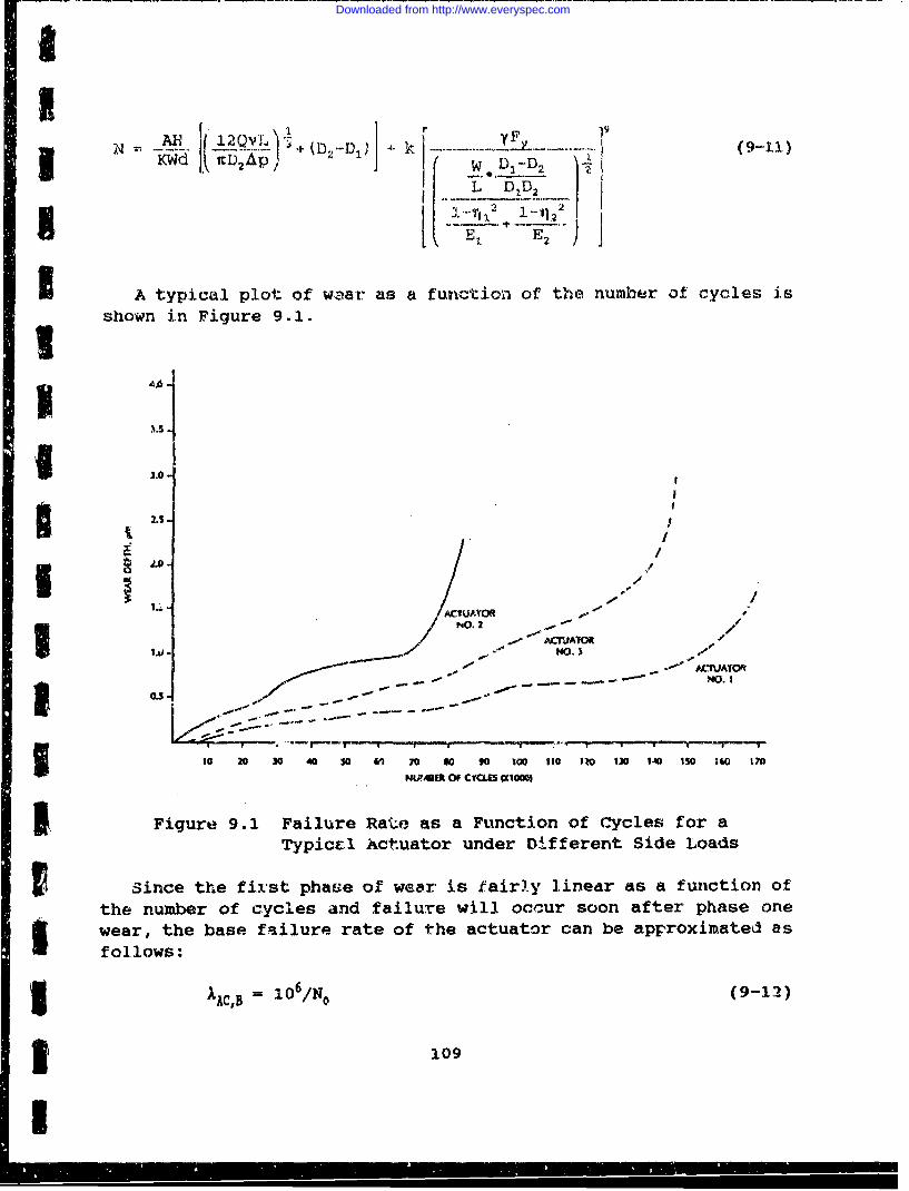
II

I D p -.J r (9-11)

Lb D1D2

I A typical plot of wear as a function of the number of cycles isshown in Figure 9.1.

"N 3.0-

AC1UATOOR

O.S.

10 20 30 40 so V 70 0 90 00 11 120 Ia M ISO 160 17

-NLVABE OF ... -"I ..

Figure 9.1 Failure Rate as a Function of Cycles for aTypical Actuator under Different Side Loads

Since the fir.st phaue of wear is fairl.y linear as a function ofthe number of cycles and failure will occur soon after phase one

iS wear, the base failure rate of the actuator can be approximated asfollows:

='•C,B = 10 6/N0 (9-12)

3 109

I


Whlere: IACB = Base Vailure rate of actuator,failures/million cycles

The complete failure rate model for the piston/cylinder actuatorincorporates modifiers for contamination and temperature effects.The complete model can be expressed as follows:

mAC = kACB cep 0 CT (9-13)

Where: AAC = Failure rate of actuator, failures/millioncycles

CC = Contaminant particle coefficient, seeSection 9.3.2

CT Temperature factor, see Section 9.3.3

9.3.2 f(ccp)During the time that the actuator is at rest, particles can work

their way 0,etween the piston and cylinder. Then, when the actuatoris put into motion, increased forces are needed to move the piston.This stiction phenomena causes a loss of actuator response and insome severe cases, a completely jammed component.

Three types of wear need to be considered in determining theeffects of contaminants on actuator reliability:

EraiQm - Particles carried in a fluid stream impact against thepiston and cylinder surfaces. If the kinetic energy released uponactuator response is large compared to forces binding thepiston/cylinder walls, surface fatigue will occur. Hard particlesmay also cut away surface material.

Abrasive Wear - A hard particle entering the gap between the pistonand cylinder surfaces can cut away material of the softer surfaceon a single actuator engagement. The rate of wear will beproportional to the number of particles in contact with thesurfaces and the particle hardness. If the hardness of the pistonis significantly less than that of the cylinder, a hard particle,absorbed by the softer material causes severe abrasive wear of theharder actuator surface.

Surface Fatigue - Particulate contaminants interacting with thepiston and cylinder surfaces can dent a surface producing plasticdeformation. Large numbers of dislocations will increa3e the

110


-NU surface roughness and deteriorate the surface material. The resultis an accelerated rate of wear and a higher probability of leakagebetween the surfaces.

The deteriorating effects of contaminant particles on thereliability of an actuator must be equated along with the

S probability of the contaminants entering the gap between theactuator surfaces. The probability of contaminants entering thisarea will depend on the operating environment, the types andI numbers of particles expected to be encountered, and the filteringsystem to prevent the entranc, of particles. The typical. actuatorcontains a bushing to wipe the piston on the return stroke. TheU life expectancy and reliability of this device must be determinedas part of the overall reliability estimate of the actuator.

If the piston surtace slides over a hard contaminant particle inthe lubricant, the surface may be subject to pitting. The abrasiveparticle has edges with a characteristic radius, denoted by r.When the depth of penetration of the abrasive particle (d) reachesa certain critical value, the scratching produces additional wearparticles by pitting. This elastic/plastic deformation processoccurs when the maximum shear stress in the complex stressdistribution beneath the contact exceeds the elastic limit. Thismaximum shear stress occurs beneath the contact at a depth equal toone half the contact radius. The value of this critical depth isgiven by (Ref. 49).

11 - 2 ff 9,max) (9-14)

d Fay

Where: fs'UX = Maximum shear stress

r = Characteristic radius of particleFsy = Yieid strength of material

If this type of wear should occur, it is so severe that actuatorperformance would be immediately effected and failure would occur.Actuators are designed to prevent particles of sufficient size tocause this type of failure and the przbability of failure from thistype of pitting is extremely low. The failure mode is presentedhere as a design evaluation check on the sealing technique for thepiston assembly.

Fatigue wear on the microscopic wear due to contaminants ist Isimilar to that for pitting just described except that it is

3 13.1


associated with individual asperity contacts rather than with asingle large region. The additional material lost due tocontaminant wear process can be estimated in the same way as theadhesive wear process was explained earlier in this chapter, thevolume 6V removed on an individual piston stroke proportional to a 3

where a is the radius of the individual area of contact.Similarly, the sliding distance 6L is proportional to A.

_6V 6A (9-15)

L- 3

Where: A = Area of contact

Summing for all contacts provides the following equation:

V L I 3 A KI - (9-16)

L1.N 3 K31 A=

Where: V = Volume of material lost due tocontaminant wear

LI = Sliding distance of the pistonN = Number of actuations

Ki = Wear coefficient

W = Transverse load on the actuatorHv = Vickers Hardness of the piston

This expression can be rewritten in the form to include acontaminant particle coefficient, C@:

V- CcpWL 1 N (917)S~Hv

The effect of the additional wear due to contaminant particlesmay be expressed as an additive term in the basic wearrelationship. It will be noted from the derivation of equationsfor the effect of contaminant particles on actuator surface wearand the possibility of stiction problems that a probability ofdamaging particles entering the gap between the piston and cylindermust be estimated. The contaminant factors involved are as

112


SI follows:H_&r-Angg$_ - The wear rate will increase with the ratio of

particle hardness to actuator surface hardness. It will normallybe the hardness of the piston that will be of concern. If theratio is less than 1, negligible wear can be expected.

umJw Q. articles - The wear rate will increase with aconcentration of suspended particles of sufficient hardness.

- For wear of the piston or cylinder to occur, the particlemust be able to enter the gap between the two surfaces. Theparticle must also be equal to or greater than the lubrication filmthickness. With decreasing film thickness, a greater proportion ofcontaminant particles entering the gap will bridge the lubricationfilm, producing increased surface damage.

.SbIpe - Rough edged and sharp thin particles will cause moredamage to the actuator surfaces than rounded particles. As theparticles remain in the gap, they will become more rounded andproduce lesr.- wear. It is the more recent particles beingintroduced ilnLo the gap that cause the damage.

SCP can be estimated by considering these variables and theirinterrelationship. The following factors can be used to estimatea value for Cap:

CI = CH CS • CN

3I Where:CW = Factor considering ratio of particle to piston

hardness, See Table 9-1.Cs = Factor considering ratio of particle size to

gap size between piston and cylinder (usefilter size/lO micronI CN = Factor considering the number of particlesmeeting hardness, size and shape parameters

I entering the qap, See Table 9-2

9.3.3 Effe !2 (CJ)3 The effect cf the temperature of the surface on the wear rate isa complicated phenomena, because the corrosion of the wear debrisat different temperatures produces different oxidation products.3Chemical interactions with the metal surfaces result in differentwear rates as the temperature of the surface is changed (Ref. 51).For example, the formation of Fe 304 is likely to predominate whensteel is subject to wear in the temperature range between 570 OF

5 113

U


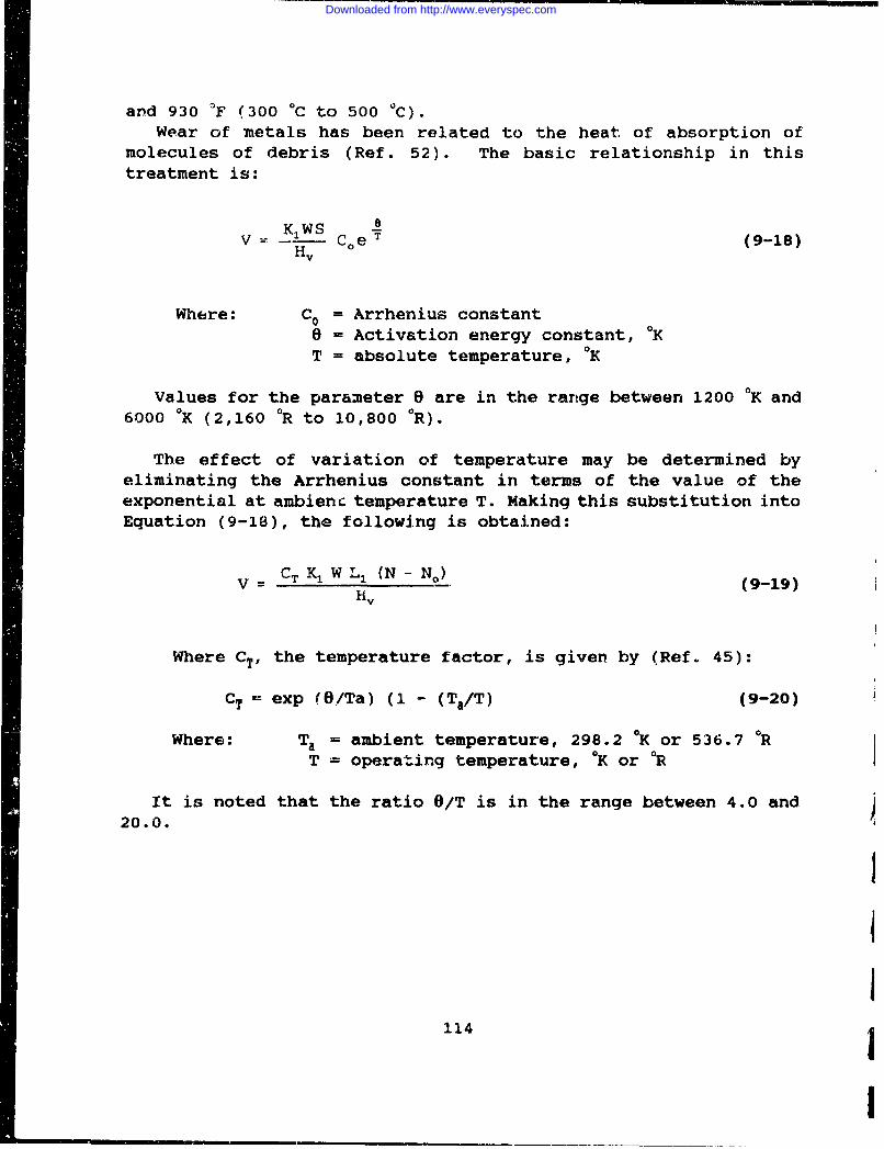
and 930 •F (300 -C to 500 OC).Wear of metals has been related to the heat of absorption of

molecules of debris (Ref. 52). The basic relationship in thistreatment is:

K1WS8"V -W Coe T (9-18)

Where: Co = Arrhenius constant0 = Activation energy constant, OKT = absolute temperature, OK

Values for the parameter 8 are in the range between 1200 0K and6000 OK (2,160 °R to 10,800 OR).

The effect of variation of temperature may be determined byeliminating the Arrhenius constant in terms of the value of theexponential at ambient temperature T. Making this substitution intoEquation (9-18), the following is obtained:

q = CT K1 W L1 (N - NO) (9-19)Hv

Where CT, the temperature factor, is given by (Ref. 45):

CT - exp (0/Ta) (1 - (Ta/T) (9-20)

Where: Ta = ambient temperature, 298.2 OK or 536.7 ORT = operating temperature, OK or OR

It is noted that the ratio 0/T is in the range between 4.0 and20.0.

114


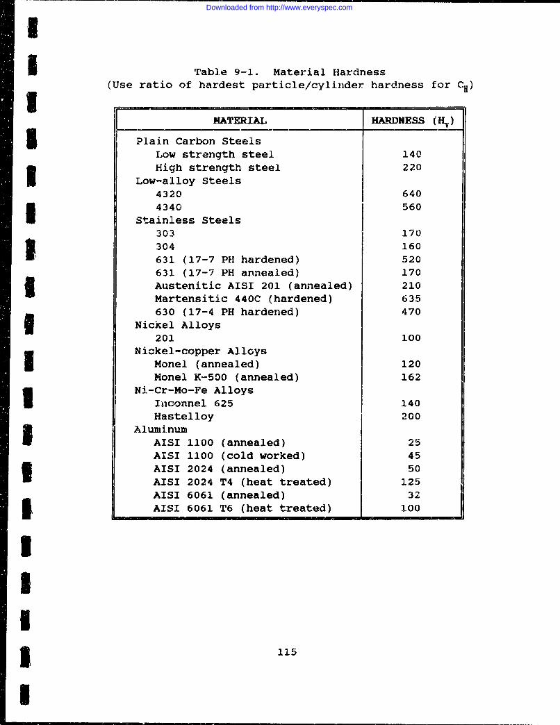
Table 9-1. Material Hardness(Use ratio of hardest particle/cylinder hardness for CH)-!-

MATERIAL HARDNESS (H)

Plain Carbon SteelsLow strength steel 140High strength steel 220I Low-alloy Steels4320 6404340 560I Stainless Steels303 170304 160631 (17-7 PH hardened) 520631 (17-7 PH annealed) 1703 Austenitic AISI 201 (annealed) 210Martensitic 440C (hardened) 635630 (17-4 PH hardened) 470

Nickel Alloys201 100

Nickel-copper AlloysMonel (annealed) 120Monel K-500 (annealed) 162

Ni-Cr-Mo-Fe AlloysInconnel 625 140Hastelloy 200

AluminumSAISI 1100 (annealed) 25

AISI 1100 (cold worked) 45AISI 2024 (annealed) 50AISI 2024 T4 (heat treated) 125AISI 6061 (annealed) 32AISI 6061 T6 (heat treated) 100

I

I-I5 115

I


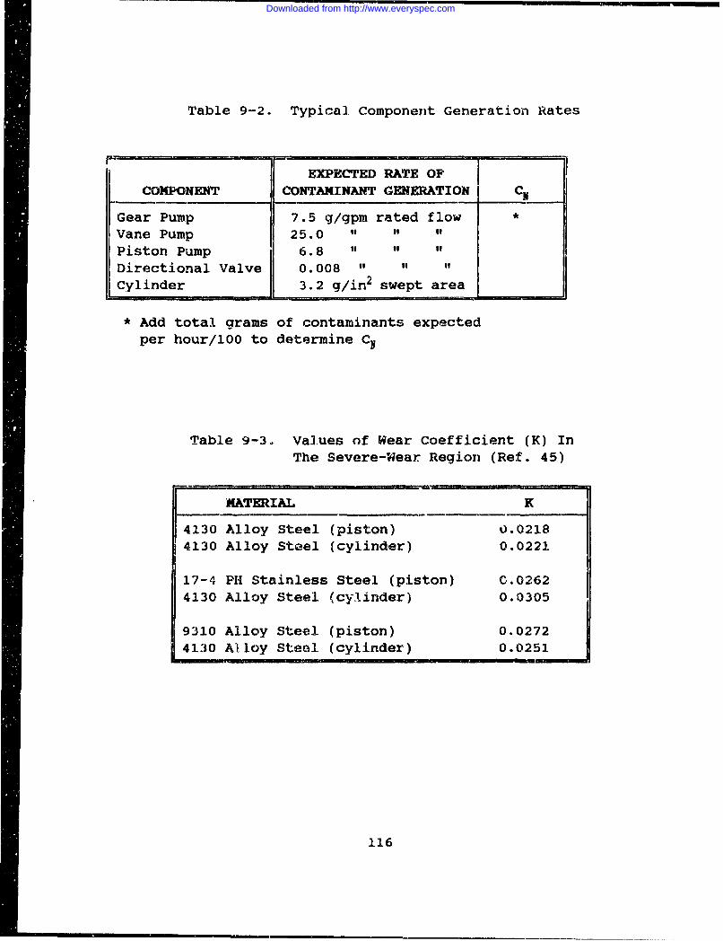
Table 9-2. Typical. Componenit Generation Rates

EXPECTED RATE OFCOMPONENT CONTAMINANT GENERATION CN

Gear Pump 7.5 g/gpm rated flowVane Pump 25.0 of of i

Piston Pump 6.8 itDirectional Valve 0.008 of

Cylinder 3.2 g/in2 swept area

*Add total grams of contaminants expectedper hour/lOO to determine C

Table 9-3. Values of Wear Coefficient (K) InThe Severe-Wear Region (Ref. 45)

MATERIAL K

4130 Alloy Steel (piston) 0.02184130 Alloy Steiel (cylinder) 0.0221

17-4 PH Stainless Steel (piston) C.02624130 Alloy Steel (cylinder) 0.0305

9310 Alloy Steel (piston) 0.02724130 A lloy Steel. (cylinder) 0.0251

116


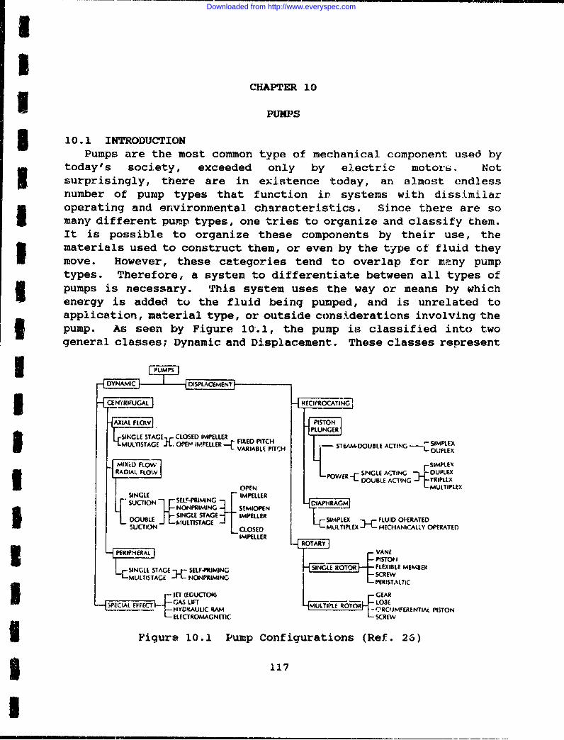
II

CHAPTER 10

UPUMPS

I 10.1 INTRODUCTIONPumps are the most common type of mechanical component used by

today's society, exceeded only by electric motors. Notsurprisingly, there are in existence today, an almost endlessnumber of pump types that function in systems with dissimilaroperating and environmental characteristics. Since there are somany different pump types, one tries to organize and classify them.It is possible to organize these components by their use, the

I materials used to construct them, or even by the type of fluid theymove. However, these categories tend to overlap for many pumptypes. Therefore, a system to differentiate between all types ofpumps is necessary. This system uses the way or means by whichenergy is added to the fluid being pumped, and is unrelated toapplication, material type, or outside considerations involving thepump. As seen by Figure 10.1, the pump is classified into twogeneral classes; Dynamic and Displacement. These classes represent

I MLTITAG JfOP IMELLR - I- SEMDOUBLE ACTING.---IPEIMUPLEX

SINLEE EA INGELLLR

4AXIN POWOW -E DUL CIG.~RP

F SELF,41RIMING IPLESUCTON •NONPRIMING . SFEMIOPEN AHAM

O S .-- INGLE STAGE CO[ IMPELLER

U LLiSTAGE O PI SI M - FLUIDOUB E AT1EICLOSED MULTIPLEX -MECHANkCALY OPERATED

SINGLEMPEELER

NGLE STAGE -cj.- SELF-PRIMING MSINGLE ROTOR FLEXIBLE MEMERIAMULISA;E. -- L. NONPRIMING LIERSTALTIC

MLITG _r FT (EDUCTOOGEA

SUCTI ONE LIOSE MULTIPLE X -ROTOR LOECHNCLYOEAE

HYDRlGAULIC RAM- C'RCUMFERENTIAL PISTON

-- ELER)GNETIC - SCREW

i Figure 10.1 Pump Configurations (Ref. 2R )

u 117

1


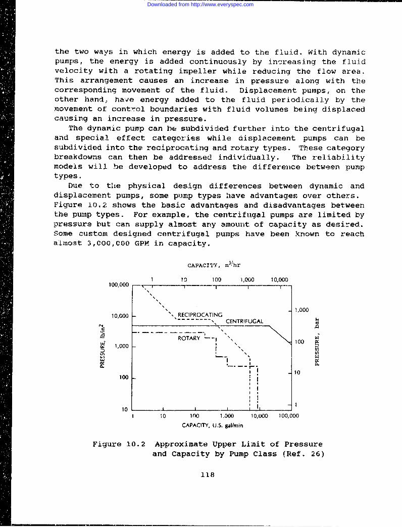
the two ways in which energy is added to the fluid. With dynamicpumps, the energy is added continuously by increasing the fluidvelocity with a rotating impeller while reducing the flow area.This arrangement causes an increase in pressure along with thecorresponding movement of the fluid. Displacement pumps, on theother hand, havie energy added to the fluid periodically by themnovement of control boundaries with fluid volumes being displacedcausing an increase in pressure.

The dynamic pump can be subdivided further into the centrifugaland special effect categories while displacement pumps can besubdivided into the reciprocating and rotary types. These categorybreakdowns can then be addressed individually. The reliabilitymodels will be developed to address the difference between pumptypes.

Due to the physical design differences between dynamic anddisplacement pumps, some pump types have advantages over others.Figure 10.2 shows the basic advantages and disadvantages betweenthe pump types. For example, the centrifugal pumps are limited bypressure but can supply almost any amount of capacity as desired.Some custom designed centrifugal pumps have been known to reachalmost 3,000,000 GPF! in capacity.

CAPACITY, m3/hr

1 13 100 1,000 10,000100,000 . 1 t ,T i

'S 1,000

10,000 S RECIPROCATING

- CENTRIFUGALC S,'

ROTARY "e 'S 1001,000

'U I

10

I

10 0

1 10 InO 1.000 10,000 100,000

CAPACITY, U.S. gal/min

Figure 10.2 Approximate Upper Limit of Pressureand Capacity by Pump Class (Ref. 26)

118


=• I

I ~Displacement pumps, however, lose capacity as the pressureincreases. It is well known that as the pump pressure increases,there is a corresponding increase in slip. The amount of slip canvary from pump to pump depending on the actual manufacturedclearances in the pump chamber. The slip can also increase withtime as wear increases.

Equation (10.1) shows that since slip "S" increases as thepressure requirements increase, the value of capacity 'IQ" is thus

3 decreased:

"g Q = (0.00433 DN) - S (10-1)

Where: Q = Capacity, GPMD = Net fluid transferred or displacedI by one cycle, ft3

N = Rotation speed (revolutions/minute)S = Slip, ft 3/min (The quantity of fluid that

escapes the full rotor cycle throughclearances or other "leak paths"

I Therefore, high pressure designs are somewhat limited to theamount of capacity, although slip can be reduced. For example, theslip can only be reduced by decreasing the tolerances to the extentthat the interference will not occur between moving parts.Interference can be a cause of extremely rapid failures.

10.2 FAILURE MODESDue to the large number of pump types and applications, someI failure modes are more prevalent than others. For example, with

displacement pumps there is a much greater chance for cyclicI •fatigue to have an effect on the system than with centrifugalpumps. This is due to the inherent difference in designs. Thedisplacement pumps have pressure transients which cause temporaryunbalanced forces to be applied to the pump and its system. Thedisplacement pump and driver shafting can experience much higherstresses during operation due to the uneven torque loading caused3 by this natural imbalance. On the other hand, the centrifugalpumps are more balanced and aren't as susceptible to large stressvariations.

Cavitation: The formation of bubbles and then the latercollapse of these vapor bubbles due to the pumps's dynamic motionis the basic definition of cavitation. In order for cavitation tooccur, the local pressure must be at or below the vapor pressure of

5 I119


the liquid. When a fluid flows over a surface having a curvature,there is a tendency for the pressure near the surface to belowered. There is a separation of fluid flow lines where there aredifferent velocity regions. Between these fluid regions,-turbulence can form which may cause bubbles to 'ccur if thepressure is low enough. The collapsing of these bubk,.es can causenoise and vibrations. Sometimes, these pressure changes can bevery dramatic and cause extensive damage to impellers, casings orshafts. If exposed for a sufficiently long time, pitting or severeerosion can occur. In some instances impeller vanes haveexperienced 3/8 inch of material loss. This type of damage cancause catastrophic failures.

Cavitation generally occurs in the first stage of a multistagecentrifugal pump, although second stages have also been found to beeffected when the suction head is substantially reduced. Withdisplacement pumps like the rotary screw, cavitation can alsooccur. For these pumps it is important to understand thecharacteristics of entrained and dissolved air with respect to thevapor pressure of the fluid medium. The rotary screw pump shows agreater tendency for cavitation when the total available pressureat the pump inlet is below atmospheric pressure. With bothdisplacement and centrifugal pumps, cavitation can be identifiedand easily remedied. Many times the inlet piping arrangement canbe modified which will cause flow patterns that alleviate theproblem.

Interference: For rotary displacement pumps, the interferenceproblem must be seriously addressed since very small distortions ofrotors will decrease the clearance causing rubbing or direct impactbetween the moving parts of the rotary displacement pump. Thermalexpansion can also pose a threat if there is no care taken in theproper selection of materials. Improper installation can also leadto interference problems. With centrifugal pumps, cavitationsignificantly increases the interference problem because cavitationcauses vibration and imbalance. Interference can be avoided bydesigning the parts from the right elastic and thermal propertiesso that excessive load or temperature won't significantly deflectinternal parts. Tolerances should be carefully adhered to.

Corrosion: Consideration must be made for other possiblefailure modes such as erosion corrosion and intergranularcorrosion. Erosion corrosion is dependent on the rate of liquidflow through the pump and also angle of attack to which the fluidimpinges on the material. Much of the knowledge for this type ofcorrosion is documented. Generally, the way in which materials

120


SI should be selected is to first determine whether there are abrasivesolids in the fluid. If there are, then the base material shouldbe selected for abrasive wear resistance; if not, then design forvelocity/corrosion resistance. Intergranular corrosion is thecorrosion of the grain boundaries of the material. For austenitic3- stainless steels, intergranular corrosion can be limited by keepingthe carbon content below 0.03 percent.

Material Fatigue: This failure mode, which cycles the materialwith unequal loadings over time, can be countered by good materials&lection. Material fatigue occurs with all types of pumps, but" may have more of an effect on displacement pumps, which have higherI fluctuating stresses.

Pump Bearing Failure Modes: The shutdown of essential equipmentcan be an expensive undertaking. Although bearings are relativelyI inexpensive, they can cause costly shutdowns of important systems.Short bearing life for centrifugal pumps, for example, can becaused by a number of troubles including the following:misalignment, a bent shaft, a rotating part rubbing on a stationarypart, a rotor out of balance causing vibration, excessive thrustcaused by mechanical failure inside the pump, excessive bearingtemperature caused by lack of lubrication, dirt or other contami-nant in the fluid, excessive grease or oil in an anti-frictionS bearing housing, and rusting of bearings from water in housing.Most of these problems can be classified by the following failuremodes: fatigue, wiping, overheating, corrosion, and wear.I Fatigue occurs due to cyclic loads normal to the bearingsurface. Wiping occurs from surface to surface contact from lossof sufficient lubrication film thickness. This can occur fromunder-rotation or from system fluid losses. Overheating is shownby babbitt cracking or surface discoloration. Corrosion isfrequently caused by the chemical reaction between the acids in thelubricants and the base metals in the babbitt. Lead based babbittstend to show a higher rate of corrosion failures.

10.3 MODEL DEVEOWPHNTThe impellers, rotors, shafts, and casings are the pump

* components which should generally have the longer lives whencompared to bearings and seals. With good designs and propermaterial selection, the reliability of impellers, rotors, andshafts should remain very high. In order to properly determinetotal pump reliability, failure rate models have been developed foreach pump component.

Pumps, just like the other mechanical components, are comprised

3 121

-I


of many component parts including: Seals, Shatt, Bearing, Casing,and Fluid Mover.

The fluid movers will be further broken down into the varioustypes common to pumps. These fluid movers can include thefollowing two general categories for centrifugal pumps: impellers;and for displacement pumps, it will be broken down into two furthersubcategories: reciprocating and rotary. For reciprocating pumpsthe fluid drivers can be classified as piston/plunger type ordiaphragm type. For rotary pumps the fluid drive is a vane typefor single rotors and for multiple rotors it is common to find agear, lobe, or screw type of fluid mover. Equation (10-2)describes the general equation for the failure rate of a pump. Thetotal pump failure rate is a combination ot the failure rates ofthe individual subcomponent parts:

IP = )SE + AK + IBE + A+ Am (10-2)

Where: ASE = Total failure rate for all pump seals,failures/million cycles (See Chapter 3)

Asp = Total failure rate for the pump shaft,failures/million cycles (See Section 10.4)

ABE = Total failure rate for all pump bearings,failures/million cycles (See Chapter 7)

ICA = Total failure rate for the pump casing,failure/million cycles (See Section 10.5)

SAF = Total failure rate for the pump fluid driver,failures/million cycles (See Section 10.6)

The order of failure rankings for typical pump subcomponentswhich vary from high to low are as follows: seals, bearings,shafta, casings and fluid drivers. The casings and drivers tend tobe replaced very infrequently. Because of this fact, emphasis willbe placed on the seals, bearings and shafts.

10.4 FAILURE RATE MODEL FOR PUMP SHAFTSThe reliability of the pump shaft itself is generally very high

when compared to other components. Studies have shown (Ref. 26)that the average MTBF for the shaft itself is over eight timesgreater than mechanical seals and over three times that of the ballbearings. The possibility that the shaft itself will fracture, orbecome inoperable is very unlikely when compared to the more commonpump failure modes. Usually the seals or bearings will causeproblems first. The effects the shaft has on the reliability of

122


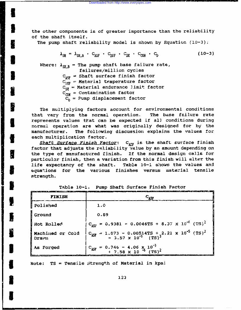
1

I Ithe other components is of greater importance than the reliabilityof the shaft itself.

The pump shaft reliability model is shown by Equation (10-3).

ISH = ISH,B " CASF CDF CSE * CM * CD (10-3)

Where: ISH,B = The pump shaft base failure rate,failures/million cycles

CAF = Shaft surface finish factorICSF onMaterial timperature factor

yCSE Material endurance limit factorCODN =Contamination factor

CD Pump displacement factor

i The multiplying factors account for environmental conditionsthat vary from the normal operation. The base failure raterepresents values that can be expected if all conditions duringnormal operation are what was originally designed for by themanufacturer. The following discussion explains the values for

I each multiplication factor.Shaft SUrfamh F a_ to CLI is the shaft surface finish

factor that adjusts the reliability value by an amount depending on3 the type of manufactured finish. If the normal design calls forparticular finish, then a variation from this finish will alter thelife expectancy of the shaft. Table 10-1 shows the values andIquations for the various finishes versus material tensilestrength.

Si Table 10-1. Pump Shaft Surface Finish Factor

FINISH cr7

Polished 1.0

Ground 0.89

Hot Rolled CAF = 0.9381 - 0.0046TS + 8.37 x 10"' (TS)'

5 Machined or Cold CIF C 1.073 - 0.00514TS + 2.21 x 10-5 (TS) 2

Drav'n - 3.57 x 10"8 (TS) 3

3 As Forged C = 0.746 - 4.06 x 10-3L 4 7.58 x 10 6 (TS) 2

E Note: TS = Tensile Strength of Material in kpsi

3 123

I


HatEral temperature o actQx: The temperature factor CDSFrepresented by Equation (10-4), is applicable for steels attemperatures greater than 160 OF. However, for temperatures below160 OF unity is used.

1S460 + TAT T > 160OF (10-4)

1

460 + TOD

Where: TOD = Design operating temperature, OFTAT = Actual operating temperature, OF

-Iaterial enduranc . 't i r: The material endurance factorwill be approximated by the factor CSE, which is the ratio ofendurance limits between what the original design specified andwhat was actually installed and used. This factor, as described byEquation (10-5), shows the relationship between the designendurance limit, SED, and the actual endurance limit, SEA.

CSE- (10-5)SEA

The endurance lirits for some common steels and alloys are shown inTable 10-2. These values may be used as inputs for Equation (10-5).

S•L m.nation factQX: The contamination factor, C0•, wasdeveloped from terearch performed for the Naval Air Warfare Centerin Warmirister, Pennsylvania on the effect of contamination andfiltration level on pump wear and performance. The contaminationfactor equation is shown below:

SCc CPAC

Where: CPAC = 0.5607 + 0.5 3 2 1FACCPDS = 0.5607 + 0.5321FD

FAC = Actual filtration level, (MABS)

124

'S


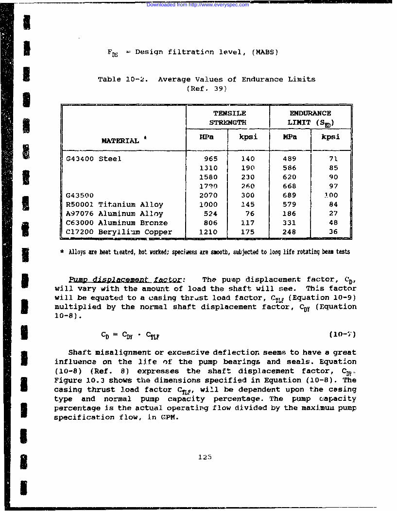
I FD = Design filtration level, (MABS)

I Table 10-2. Average Values of Endurance Limits(Ref. 39)

TENSILE ENDURANCESTRENGTH LIMIT (Sm)

MATERIAL* HPa kpsi MPa kpsi

G43400 Steel 965 140 489 711310 190 586 851580 230 620 901790 260 668 97

G43500 2070 300 689 100R50001 Titanium Alloy 1000 145 579 84A97076 Aluminum Alloy 524 76 186 27C63000 Aluminum Bronze 806 117 331 48C17200 Berylliun Copper 1210 175 248 36

~J'-

3lloys are beat tAeated, bo. worked; speciens are sooth, subjected to long life rotating bea tests

Ldr,=: The pump displacement factor, CD,will vary with the amount of load the shaft will see. This factorwill be equated to a casing thrast load factor, CT• (Equation 10-9)multiplied by the normal shaft displacement factor, CDy (Equation10-8).

I CD = CDYC (O-i')

Shaft misalignment or excescive deflection seems to have a greatinfluence on the life of the pump bearings and seals. Equation(10-8) (Ref. 8) expresses the shaft displacement factor, CDY..

i Figure 10.3 shows the dimensions specified in Equation (10-8). Thecasing thrust load factor CT, will be dependent upon the casingtype and normal pump capacity percentage. The pump capacityU percentage is the actual operating flow divided by the maximum pumpspecification flow, In GPM.

13 125

I


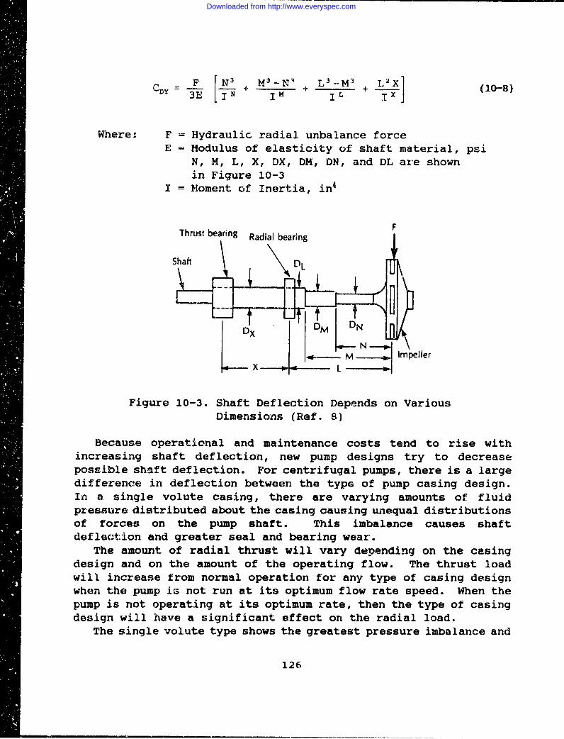
=-DY - + + + + (10-8)3 I NI K i L TIx

Where: F = Hydraulic radial unbalance forceE = Modulus of elasticity of shaft material, psi

N, M, L, X, DX, DM, DN, and DL are shownin Figure 10-3

I = Moment of Inertia, in 4

S~F

Thrust bearing Radial bearing

Shaft L

DX DM DN

- M Impeller

Figure 10-3. Shaft Deflection Depends on VariousDimensions (Ref. 8)

Because operational and maintenance costs tend to rise withincreasing shaft deflection, new pump designs try to decreasepossible shaft deflection. For centrifugal pumps, there is a largedifference in deflection between the type of pump casing design.In a single volute casing, there are varying amounts of fluidpressure distributed about the casing causing unequal distributionsof forces on the pump shaft. This imbalance causes shaftdeflection and greater seal and bearing wear.

The amount of radial thrust will vary depending on the casingdesign and on the amount of the operating flow. The thrust loadwill increase from normal operation for any type of casing designwhen the pump is not run at its optimum flow rate speed. When thepump is riot operating at its optimum rate, then the type of casingdesign will have a significant effect on the radial load.

The single volute type shows the greatest pressure imbalance and

126


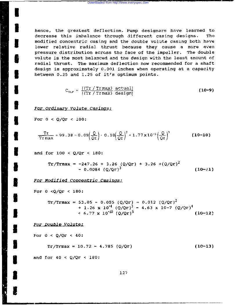
I hence, the greatest deflection. Pump designars have learned todecrease this imbalance through different casing designs. Themodified concentric casing and the double volute casing both havelower relative radial thrust because they cause a more evenpressure distribution across the face of the impeller. The doublevolute is the most balanced and the design with the least amount ofradial thrust. The maximum deflection now recommended for a shaftdesign is approximately 0.001 inches when operating at a capacitybetween 0.25 and 1.25 of it's optimum points.

CTLF = [(Tr/Trmax) actual] (10-9)[(Tr /Trmax) design]

I For Ordinary Volute Cas•ingý

5 For 0 < Q/Qr < 100:

Tr -99.38 -0.09 0 . o0-2--2+ 1.717xo- 3 (10-10)Txmax ) (Q

5 and for 100 < Q/Qr < 180:

Tr/Trmax = -247.26 + 3.26 (Q/Qr) + 3.26 +(Q/Qr) 2

- 0.0084 (QQr)(0-)

I FQ~~eQd Conh•

For 0 <Q/Qr < 180:

Tr/Trmax = 53.05 - 0.055 (Q/Qr) - 0.012 (Q/Qr) 2

+ 1.26 x .0-4 (Q/Qr) 3 - 4.63 x 10-7 (Q/Qr) 4

+ 4 6.77 x 10"11 (Q/Qr)5 (10-12,

For 0 < Q/Qr < 40:

U Tr/Trmax = 1.0.72 - 4.785 (Q/Qr) (10-13)

3 and for 40 < Q/Qr < 180:

3 127


Tr/Trmax = 14.292 - 0.297 (Q/Qr) + 4.11 x 101 (Q/Qr) 2 (10-14)

Where: Q = Actual operating flow, gpmQr = Maximum pump specification flow, gpm

10.5 FAILURE RATE MODEL FOR IMP1MLLER1, CASINGS, AND ROTORSThe pump casing is A very reliable component. Defined as A•, the

case will have a greater effect on total pump reliability from thestandpoint of how it effects other less reliable components. Forinstance, for an ANSI pump, the casing may have an average lifeexpectancy of 10 years where a seal or bearing may have only one ortwo years. However, the type of casing used in the pump can havea large effect on the lifetime of the bearings and seals. This isdue to differing loads placed on the pump shaft by the fluid flowpattern. The fluid flow patterns are a function of the casingdesign. As shown in the following equations, the thrust will varywith the type of casing design and the pump flow rate. The valuefor reliability of the pump casings (A•) themselves will bepresently equated to .0001 failures/million cycles.

10.6 FAILURE RATE ESTIMATES FOR FLUID MOVERSAll pumps require some vehicle to move the fluid from the

intakes and expel it through the volutes to the exhaust opening.The means by which pumps do this is what differentiates most oftoday's numerous types of pumps. The reliability of these fluidmovers will vary from pump to pump. Impellers will wear out longafter the seals. Pump gears for rotary gear pumps will have alower reliability than impellers due to the nature of the contactbetween goears and the speed they attain.

Piston-plunger displacement pumps will generally have largerwear rates for the piston walls and rings than for the impellers ofcentrifugal pumps. The following average failure rates have beendetermined from data base information developed from the Navy.

The equations that describe the "fluid driver" wear rate mayvary drastically since th3 "fluid driver" varies greatly in designand application. See Table 10-3 for the general categories for thefluid driver.

Since there are many types of fluid drivers, many reliabilitymodels are required to be developed. However since little data isavailable for each model, a base failure rate can be used toquantify these variations until fully developed models areestablished. Failure of the fluid drivers themselves are much lesslikely than failures of the other subcomponent pump parts.

128


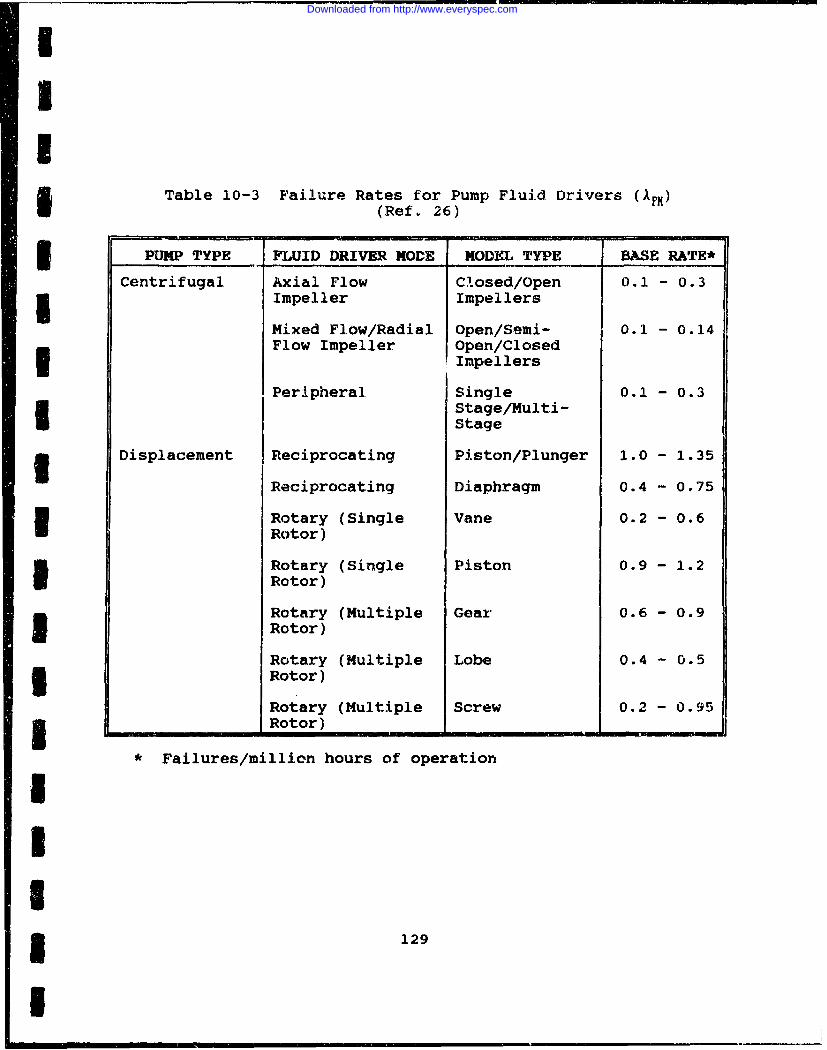
I

Table 10-3 Failure Rates for Pump Fluid Drivers (AFM)(Ref. 26)

5 PUMP TYPE FLUID DRIVER MODE MODEL TYPE BASE RATE*

Centrifugal Axial Flow Closed/Open 0.1 - 0.33 Impeller Impellers

Mixed Flow/Radial Open/Semi- 0.1 - 0.14Flow Impeller Open/Closed

Impellers

Peripheral, Single 0.1 - 0.3Stage/Multi-Stage

3 Displacement Reciprocating Piston/Plunger 1.0 - 1.35

Reciprocating Diaphragm 0.4 - 0.75

Rotary (Single Vane 0.2 - 0.6Rotor)

Rotary (Single Piston 0.9 - 1.2I Rotor)

Rotary (Multiple Gear 0.6 - 0.9Rotor)

Rotary (Multiple Lobe 0.4 - 0.5* Rotor)

Rotary (Multiple Screw 0.2 - 0.953 Rotor) .... _ ,,-

* Failures/million hours of operation

II33 129

I



lao


I

U CHAPTER 1 1

FILTERS

11.1 INTRODUCTIONFluid filtration equipment is unique in that the reliability of

this equipment is more concerned with the effects of the filter onassociated equipment than on the lifetime of the filter itself.This is due to severe wear of fluid system ccmponents which canoccur when these components are operated with poorly filtered

I fluid. This chapter will review the conditions which can lead todegradation or failure of the filter. The effects of contaminationon the wear of various components is also discussed. A basicfailure rate model with correction factors will also be developed.

11.2 FILTRATION MECHANISMSFilters are constructed of a porous filter media through which

fluid is passed. The filter media is typically corrugated toincrease the amount of filtration area in the filter volume.

I Filtration of gases is accomplished by absorption and directinterception of the suspended particles. Filtration of liquids isprimarily accomplished by direct interception of the suspended

I particles.

11.3 SERVICE LIFEThe porous structure of a filter media presents a resistance to

fluid flow which causes 4 pressure drop across the filter. Thisfilter differential pressure increases as captured particles orcontaminants are collected and plug the porous media. Every systemhas a maximum differential pressure at which the filter must beU cleaned or replaced. The filter service life is the time it takesthe filter to reach the maximum allowable differential pressure.Use of the filter beyond its service life could result in

I catastrophic failure of the filter due to the high differentialpressure or it could result in unfiltered fluid bypassing thefilter (Ref. 33)

11.4 FILTER FAILUREA filter is considered to have failed when it releases

previously captured contaminants, when it allows unfiltered flui,-

5 131

U


to pass throughout the filter media, or when the filter collapsesand contaminates the fluid with filter media. Plugging of thefilter with contaminants, with a resulting increase in filterdifferential pressure, is a normal consequence of operation and isnot considered a failure even if it occurs prematurely. Failure ofthe filter can be caused by operating conditions such as highdifferential pressures, cyclic flow, vibration, system startupswhen cold, and even the fluid being filtered, if the fluid isincompatible with the filter.

11.5 FILTER FAILURE MODESh hanngeling: Excessively high differential pressures can cause

filter media pores to enlarge, allowing large amounts of unfilteredfluid to bypass the filter media. Enlargement of the media poresalso allows previously captured contaminants to be released.Channelling can also be the result of media fatigue caused bycyclic flow conditions.

Fatigu&_QCracks Cyclic flow conditions in the fluid system cancause fatigue cracks in the filter media. Such cracks may occur atthe roots of pleats in corrugated filters or within the volume ofloose packed media. The cracks will allow the release ofcontaminants from the filter and will allow some of the fluid tobypass the filter. Media fatigue can result from cyclic flowconditions such as varying system flow requirements, pump ripple,or cold system startups.Hii Migr-dtn: Improper bonding of the media fibers or

deterioration of the bonding can result in the down stream releaseof media fibers. This downstream release of the filter media istermed media migration. Media migration during vibration of thefilter may result from an improper fit of the filter in the filterhousing or may result from the filter media abrading against thefilter casing. Media migration can also occur in conjunction withfatigue cracks in the media, as caused by cyclic flow conditions.Media migration can also occur during cold temperature start-upsdue to potential large differential pressure generated as aconsequence of increased fluid viscosity.

Filter Disintegrati.on Complete disintegration of the filtercan occur as a result of extremely high differential pressures.Disintegration can also be the result of embrittlement of thefilter media from exposure to incompatible fluids or coldtemperatures.

F£uging; Plugging of the filter media can be either a normalconsequence of operation or failure, depending upon when plugging

132


I

I occurs. Failure due to premature plugging can be attributed toseveral causes other than just the accumulation of wear debris. As

I an example, Hudgens and Feldhaus (Ref. 24) have found thatlubrication oil filters in diesel engines can plug by any one ofsix mechanisms. While some of these are particular to internalcombustion engines, the mechanisms may be applicable to anyoil-based fluid system. The six mechanisms can be summarized asfollows:

1. Absorption of water in the oil from condensed moistureand/or coolant leakage can cause insoluble contaminants, normallydispersed into the lubricating oil, to dump out of suspension.This condition can also arise when there is a combination ofmoderate soot load, low pH and a high level of oxidation producedU in the oil. A filter plugged under these circumstances will bemarked by a sticky, shiny, adherent sludge with wavy pleats and thefilter will have accumulated from 1/3 to 1/2 of its totalcontaminant capacity.

2. Saturation of the oil with excessive amounts of combustioncontaminants, due to engine problems or overextended oil drain

I internals, can also cause filter plugging. The filter will appearto have a thick, loosely-held sludge. The filter will haveaccumulated from 1/3 to 1/2 of its total contaminant capacitytypically but it can accumulate up to 100 percent in extreme cases.

3. Absorption of oxidation products such as degraded fuel andoil will also cause the filter to plug and the filter will haveaccumulated 40 percent to 50 percent of its contaminant capacity.The filter does not appear to have sludge buildup but it doesappear to have a brown tint and to be covered by blown snow. Theproblem occurs most often with API CC spec lubricating oils whereoverheating or fuel dilution is a problem.

4. Moisture condensation or coolant leakage into the oilreservoir can cause filters to plug as a result of oil additiveprecipitation. Plugging of the filter can occur at 8 percent to 30I percent of the filter's contaminant capability. The filter willhave a gray coloration but no sludge build up.

5. Coolant or moisture can also combine with oil additives toI form thick, filter-plugging gels. The filter media in such

circumstances will be wavy with a sticky feel but will usually lookclean. Filters plugged due to gel formation usually reach only 33 percent to 6 percent of their contaminant capacity before plugging.

6. Accumulation of wear debris also causes filters to plug. Inthis failure mechanism, the filter plugs by retention of 100percent or more of its full contaminant capacity. The filter will

* 133

.3


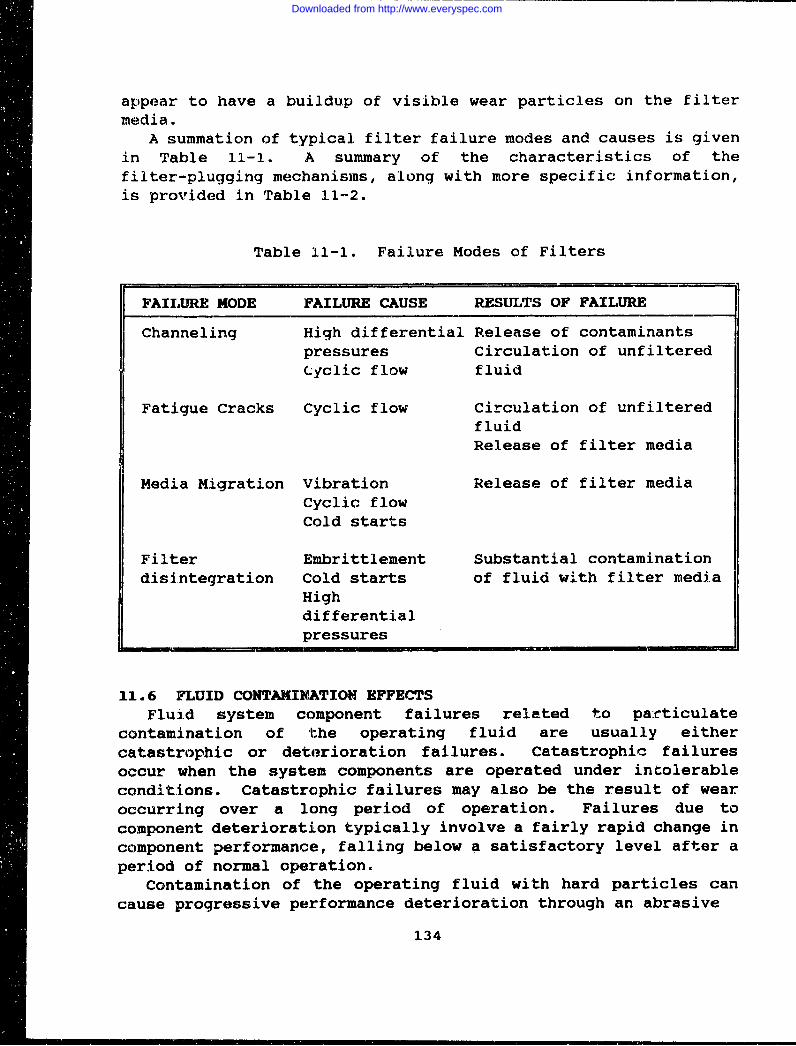
appear to have a buildup of visible wear particles on the filtermedia.

A summation of typical filter failure modes and causes is givenin Table 11-1. A summary of the characteristics of thefilter-plugging mechanisms, along with more specific information,is provided in Table 11-2.

Table il-i. Failure Modes of Filters

FAILURE MODE FAILURE CAUSE RESULTS OF FAILURE

Channeling High differential Release of contaminantsSpressures Circulation of unfiltered

Cyclic flow fluid

Fatigue Cracks Cyclic flow Circulation of unfilteredfluidRelease of filter media

Media Migration Vibration Release of filter mediaCyclic flowCold starts

Filter Embrittlement Substantial contaminationdisintegration Cold starts of fluid with filter media

Highdifferentialpressures

11.6 FLUID CONTAMINATION EFFECTSFluid system component failures related to particulate

contamination of the operating fluid are usually eithercatastrophic or deterioration failures. Catastrophic failuresoccur when the system components are operated under intolerableconditions. Catastrophic failures may also be the result of wearoccurring over a long period of operation. Failures due tocomponent deterioration typically involve a fairly rapid change incomponent performance, falling below a satisfactory level after aperiod of normal operation.

Contamination of the operating fluid with hard particles cancause progressive performance deterioration through an abrasive

134


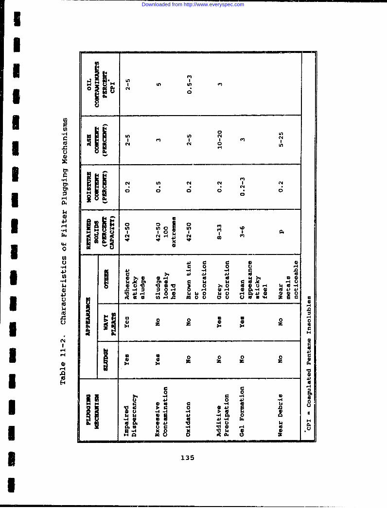
In

kn In

1r 0 In.9A in NJ N'

.00

I . vi C4

V 0 0 0 d040

.49 914 in in in

I6I1 1~ 0

0 '

-r0 0 04 J -- 4 - _ _ _ 0

ý4 doI1 Mo 0 0 0 dV4) r P4 14 -4 1 '

to 0 0 0 0 0

0 0 0

q-4 0 0 04

.4

00 4

-4 '-4-4 W -A 0

135


wear mechanism. This type of wear is characterized by a particlepenetrating a softer surface and cutting away material. The rateof wear and thus the rate of performance degradation is dependenton the number of particles and the particle hardness. Particlecontamination can also cause cumulative performance degradationwhere a rapid decline in performance follows an extended period ofapparently normal operations. This type of degradation failure iscaused by the creation of surface defects during operation. Thesesurface defects may be caused by abrasion, surface fatigue oradhesion wear processes.

Fluid systems requiring filtration typically include componentssuch as pumps, gears, control valves, ball bearings, rollerbearings, journal bearings, and seals.

P In displacement-type piston pumps, the piston face canbe damaged by cavitation or corrosion. Contaminant pazticles canenter the lubricant film between the piston and cylinder and ploughthe surface several times before being ejected. In swashplatecontrolled devices, such as variable displacement pumps andhydraulic motors, the piston shoes can cause abrasion-wear-typedegradation failures as the shoes are highly loaded and are insliding contact with the swashplate. Similar abrasive-wear-typedegradation failures can occur to the sliding contact surfaces ofthe rotating cylinder block and the mating valve pressure plates(Ref. 7)

QVar,&L Gear failures are primarily failures of the gear toothsurface. This surface is damaged by rubbing wear, scoring,pitting, and plastic flow. Rubbing wear occurs when the lubricantfilm is insufficient to separate the tooth surfaces and isgenerated by both adhesive and abrasive wear mechanisms. Scoringof the tooth surface is generated by the adhesive wear typemechanisms under intense local frictional heating. Pitting andplastic flow both occur as a result of tooth surface fatigue wear(Ref. 7)

y Particle contamination can cause increased leakage incontrol valves by severe cutting or by milder abrasive wearmechanisms. Synthetic phosphate ester fluids have been found tocause servo valve erosion by a streaming-potential corrosionprocess. A brittle corrusion layer is formed on the valve and isabraded by fluid-borne particles, adding additional particulates tothe fluid and exposing base metal, allowing further corrosion.Deterioration failures of relief valves can occur from particlecontamination caused by erosion. Contamination of hydraulic fluid

136


SI by water has been shown to cause rust inhibitor additive to attachto servo valve spools and prevent movement of the valve spoolwithin its housing (Ref. 7).I iZlqxc •_;_~ Hard particle cont.mination of ball and rollerbearing lubricants is the cause of two types of abrasive wear ofthe rolling surfaces. Hard particle contamination causes rollingsurface damage that dominates the fatigue life of ball bearingsunder typical operating conditions. In severe circumstances, hard3 particle contamination causes indentations and pits which causerapid failure of the rolling surfaces. Abrasive wear, increasingwith particle concentration and hardness, can remove material fromthe sliding edges of a tapered rolling bearing, reducing thebearing width and allowing increased misalignment. Wear of thistype does not stop until the contaminant size is reduced to lessI than the lubricant film thickness.

The performance of new journal bearings improves with useinitially due to better surface conformity caused by wear during

Sboundary lubrication conditions. As wear in the contact regionprogresses, the performance begins to gradually deteriorate. Wearof the journal bearings is caused by both abrasive and adhesivewear due to the sliding motion in the contact region.Contamination of the lubricant with water can cause the formationof a metal oxide boundary layer on the bearing which can inhibitadhesive wear. However, abrasion of this film can cause bearingfailure due to rapid increases in wear, bearing corrosion, and thenumber of abrasive oxide particles. Maximum bearing life can beachieved by selecting a filter to filter cut all particles largerthan the minimum lubricating film thickness. (Ref. 7).I eLAI Seal failures are typir-Ally caused by fatigue-likesurface embrittlement, abrasive removal of material, andcorrosion. Elastomeric seals are more sensitive to thermaldeterioration than to mechanical wear, However, hard particles canbecone embadded in soft elastomurc materials and sliding contactmetal surfaces, carsing leakage U:y abrasive wear of the hardermating surfaces. Abrasive particles can also plug lubricantpassages which causes seal failure frcm the lack of lubricant.Seal failures can be reduced ')y reducing the amount ofcontamination through filtration ind concern for the operatingenvircnmjnt (Ref. 7).

"11.7 RELIABILITY MODELA basiL. filter reliability 'odel can be developed by modeling

the fluid system incorporating the filter. By modeling the flow of

3 I137


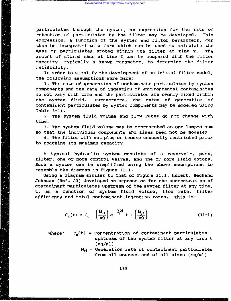
particulates through the system, an expression for the rate ofretention of particulates by the filter may be developed. Thisexpression, a function of the system and filter parameters, canthem be integrated tc a form which can be used to calculate themass of particulates stored within the filter at time T. Theamount of stored mass at time T can be compared with the filtercapacity, typically a known parameter, to determine the filterreliability.

In order to simplify the development of an initial filter model,the following assumptions were made.

1. The rate of generation of contaminate particulates by systemcomponents and the rate of ingestion of environmental contaminatesdo not vary with time and the particulates are evenly mixed withinthe system fluid. Furthermore, the rates of generation ofcontaminant particulates by system components may be modeled usingTable 3-11.

2. The system fluid volume and flow rates do not change withtime.

3. The system fluid volume may be represented as one lumped sumso that the individual components and lines need not be modeled.

4. The filter will not plug or become unusually restricted priorto reaching its maximum capacity.

A typical hydraulic system consists of a reservoir, pump,filter, one or more control valves, and one or more fluid motors.Such a system can be simplified using the above assumptions toresemble the diagram in Figure 11.1.

Using a diagram similar to that of Figure 11.1, Hubert, BeckandJohnson (Ref. 23) developed an expression for the concentration ofcontaminant particulates upstream of the system filter at any time,t, as a function of system fluid volume, flow rate, filterefficiency and total contaminant ingestion rates. This is:

Cu(t) = CO - tQ e - t +ý (Q] (11-1)

Where: Cu(t) = Concentration of contaminant particulatesupstream of the system filter at any time t(mg/ml)

Mc1 = Generation rate of contaminant particulatesfrom all sources and of all sizes (mg/ml)

138


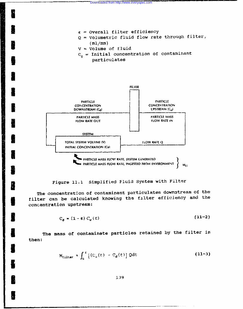
U

I = Overall filter efficiencyQ = Volumetric fluid flow rate through filter,

I (n fmi/mm)

V = Volume of fluidCo = Initial concentration of contaminant

particulates

I3 FIL(ER

PARTICLE PARTICLE

CONCENTRATION CONCENTRATIONDOWNSTREAM (Cd) UPSTREAM (Cu)

PARTICLE MASS PARTICLE MASS- FLOW RATE OUT FLOW RATE IN

SYSTEM

TOTAL SYSTEM VOLUME (V) f LOW RATE Q

INITIAL CONCENTRATION (Co)

N1 4 PARTICLE MASS FLOW RATE, SYSTEM CENERATEDS4 rPARTICLE MASS FLOW RATE, INGESTED FROM ENVIRONMENT i Mci

Figure 11.1 Simplified Fluid System with Filter

The concentration of contaminant particulates downstream of the

I filter can be calculated knowing the filter efficiency and the

concentration upstream:

I Cd = (i- e) Cu(t) (11-2)

I The mass of contaminate particles retained by the filter is

then:

r= f0 [(c(t) - Cd(t)] Qdt (11-3)

1.39

I


Substituting Equation (11-2) into Equation (11-3) yields:

Mfilter = fo Cu(t) Qdt (11-4)

and substitution of Equation (11-1) into Equation (11-4) yields:

t-cQT1MfLlter = J [(E Q CO - Mi) e + Mcji dt (11--)

This is then integrated to yield the following expression of theretained mass as a function of time:

- eQt

Mtliter = (CQC. - M,,) (e v - 1) + Meit (1t-6)

Knowing the system parameters and the filter contaminantcapacity, the filter lifetime can be calculated on atrail-and-error basis using (note the presence of the variable t onboth sides of the equation):

t n[FCC + eqco -- Mci(1-t) (11-7)

Where: FCC = Contaminate capacity of the filter (mg)t = Lifetime in minutes

Solution of Equation (11-7) for t yields a base service lifet which can be used to calculate the base failure rate for thefilter:

__XF.B :(6.0 x 107) (11-8)F. B t

Where: IFB = Base failure rate of a filter in normaloperation (failures/million hours)

140


I The complete filter failure rate model should use adjustments,or correction factors, to modify the base failure and to account

* for potentially degrading effects of off-design operatingconditions. Considering the causes of failures as earlierdiscussed, the tailure rate model is:

x F• * CDPa C V• S CCS * CF. * CT (11-9)

Where: AF = Failure rate of the filter infailures/million hoursI XF,B = Base failure rate of the filter infailures/million hours

SCD= Multiplying factor which considersthe effects of the filter differentialpressure on the base failure rate

CCF= Multiplying factor which considersthe effects of cyclic flow on thebase failure rate

CV = Multiplying factor which considersthe effects of vibration on thebase failure rate

CCS = Multiplying factor which considersthe effects of cold start-up conditionson the base failure rate

CE = Multiplying factor which considersthe effects of incompatible fluids andmaterials on the base failure rate

CT = Multiplying factor which considersthe effects of temperature on the base

3 failure rate

Assuming that the filter may be modeled as a thick-walledcylinder, the correction factor for filter differential pressure(Ct) may be developed from the following equation for radial stress(Ref.39).

Pi a2 - P, a2 b2 (p0 -

a 2br 2 b a 2 r 2I 0

I3 141

-


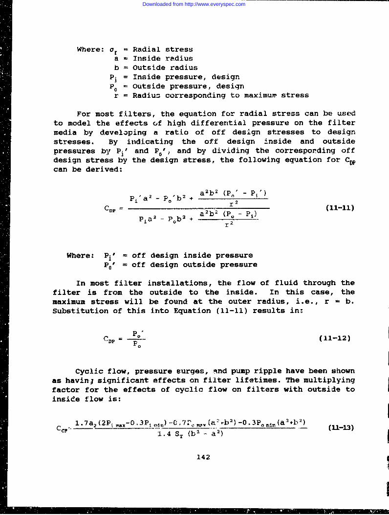
Where: ar = Radial stressa - Inside radiusb = Outside radiusP1 = Inside pressure, designP0 = Outside pressure, design

r = Radius corresponding to maximuim stress

For most filters, the equation for radial stress can be usedto model the effects Gf high differential pressurea on the filtermedia by developing a ratio of off design stresses to designstresses. By indicating the off design inside and outsidepressures by Pi' and P01, and by dividing the correspording offdesign stress by the design stress, the following equation for CDcan be derived:

2- P 'b 2 + a 2 b 2 (Po' - Pi')

CP= 2________ 2 (11-11)

Pi a2 - pob2 +

r2

Where: Pi" = off design inside pressurePO' = off design outside pressure

In most filter installations, the flow of fluid through thefilter is from the outside to the inside. In this case, themaximum stress will be found at the outer radius, i.e., r = b.Substitution of this into Equation (Il-il) results in:

C Po"pa (11-12)CDP =P

Cyclic flow, pressure surges, And pump ripple have been shownas havinj significant effects on filter lifetimes. The multiplyingfactor for the effects of cyclic flow on filters with outside toinside flow is:

- 1.7a 2 (2PlX-O.3P4 ,in)-C-71oMt?,Va 2 ,b 2 )-O.3PO i. (a)+b')1.4 ST (b 2 ,- a 2 )

142


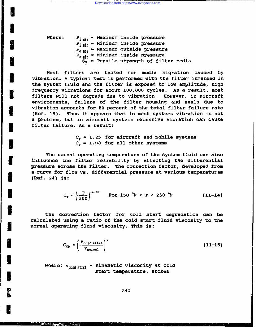
IIWhere: Piax = Maximum intside pressure

Piin = Minimum inside pressurePO Sx = Maximum outside nressurePoain = Minimum inside pressure

ST -- Tensile strength of filter media

Most filters are tes3ted for media migration caused byvibration. A typical test is performed with the filter immersed inthe system fluid and the filter is exposed to low amplitude, highfrequency vibrations for about 100,000 cycles. As a result, mostfilters will not degrade due to vibration. However, in aircraftenvironments, failure of the filter housing and seals due tovibration accounts for 80 percent of the total filter failure rate(Ref. 15). Thus it appears that in most systems vibration is nota problem, but in aircraft systems excessive vibration can causefilter failure. As a result:

CV = 1.25 for aircraft and mobile systemsSCv = 1.00 for all other systems

The normal operating temperature of the system fluid can also3 influence the filter reliability by affecting the differentialpressure across the filter. The correction factor, developed froma curve for flow vs. differantial pressure at various temperatures(Ref. 24) is:

CT T- .9 For 150 9F < T < 250 aF (11-14)

I The correction factor for cold start degradation can becalculated using a ratio of the cold start fluid viscosity to the3 normal oerating fluid viscosity. This is:

iC = (C Vc1d start) (11-15)

Where: voldstrt ' Kinematic viscosity at coldstart temperature, stokes

143

I


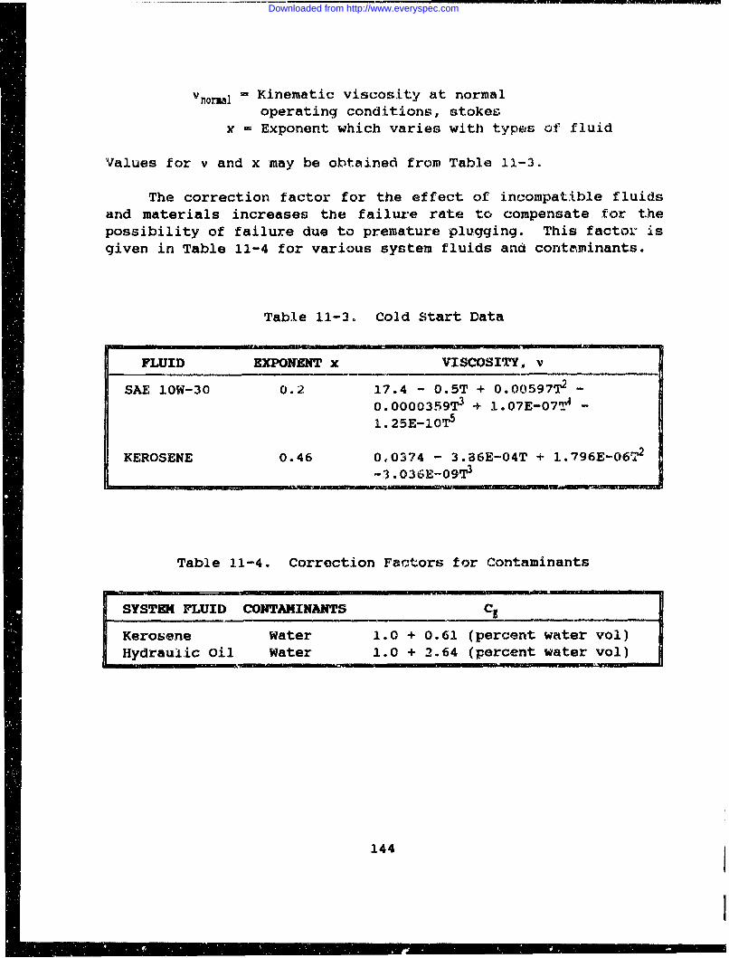
•m 2MM

Vnonal- Kinematic viscosity at normaloperating conditions, stokes

x = Exponent which varies with types of fluid

Values for v and x may be obtained from Table 11-3.

The correction factor for the effect of incompatible fluidsand materials increases the failure rate to compensate for thepossibility of failure due to premature plugging. This factor isgiven in Table 11-4 for various system fluids and contaminants.

Table 11-3. Cold Start Data

FLUID EXPONENT x VISCOSITY, v

SAE 1OW-30 0.2 17.4 - 0.5T + 0.00597 2 -

0.0000359T3 + 1.07E-07T4 -

.1. 25E-10115

KEROSENE 0.46 0.0374 - 3.86E-04T + 1.796E-06.,

-3.036E-09T3

Table 11-4. Correction Factors for Contaminants

SYSTEM FLUID CONTAMINANTS CE

Kerosene Water 1.0 + 0.61 (percent water vol)Hydraulic Oil Water 1.0 + 2.64 (percent water vol)

144


I

CHAPTER 12

BRAKES AND CLUTCHES

12.1 INTROI'UCTIONThe principal function of a brake or clutch assembly is to

convert kinetic energy to heat and then either to absorb ordissipate heat while simultaneously (through energy transfer)I reducing the relative movement between the friction material andthe part to which it is engaged. Reliability models for brakes andclutches are presented together in this Handbook because of similardesign and operational characteristics; and because one of the mostimportant functional parts of each of these components is thefriction material. Section 32.2 addresses the brake model, whichincludes actuators, springs, friction linings, bearings, seals andhousings. An analysis of the energy transfer materials which arecommon to both brakes and clutches is included in the brake model.Section 12.3 outlines and describes the reliability model forclutches, which includes the following subcomponents: actuators,bearings, friction linings, seals and springs.

I 12.2 BRAKES

12.2.1 Brg ,%R•jg

The reliability of a brake system is dependent on thereliability of its parts, which may include: actuators, bearings,friction linings, housings, seals, and springs. With the exceptionof friction linings, all these component parts are addressed inearlier sections of this handbook. The characteristics of theseparts that are peculiar to the braking environment will bediscussed in this section. Because friction materials are uniqueto brake and clutch components, an in depth analysis of thesemechanical parts is presented in this section cf the handbook.

In brake systems the rubbing elements include the frictionmaterial and a countersurface. The friction material is thesacrificial element, although the essence of good brake design isto minimize wear. The countersurface is usually metallic, toprovide structure and to dissipate the frictional heat. Mostcountersurfaces are a grey cast iron drum or disc. In a fewapplications, steel rubbing surfaces are used. The countersurface

145

I== _


is also nominally a non-wearing surface. Countersurfaces typicallywear from 1 to 20 percent of the total volume worn from thefriction interface (Ref. 16).

Brakes are called upon to convert large amounts of kineticenergy to thermal energy in a very short time. The life ofcurrently used brake lining materials is determined by wear, whichin turn is strongly dependent on the temperature experienced bythese materials during sliding. This temperature dependence i.s duelargely to softening of the metal binder (usually copper or .-ron)present in brake lining composite materials.

Some of the systems which use brakes include, passenger cars,light trucks, tractors, buses, agricultural equipment, constructionequipment, industrial equipment, railroad trains and aircraft.Brake lining materials used in passenger cars and light trucks fallinto two categories: drum brake segments, which are less than 3/4"thick, and disk brake pads.

Brake systems used by trucks, truck tractors, and trailercombinations are air assisted hydraulic (air brake) systems. Thebraking systems used by buses are similar to the conventional airbrake system used by large trucks. Brake linings are almostentirely brake blocks used by the drum brake system. Conventionallinings create excessive drum wear.

Agriculturbl, construction and industrial equipment each havedifferent brake requirements. Agricultural equipment includes allequipment used in farming and forestry, such as tractors,harvesters, and log skidders. Construction equipment is used forthe construction of roads, homes and buildings and includ6s wheeledtractors, rollers, scrapers, dozers, power truck cranes, hoists andshovel lodders. Industrial equipment encompasses all equipmentused ijA fixed facility or buildings such as overhead cranes orhoists.

Hydraulic brake systems used in agricultural and constructionequipment are of either the dry or the wet brake type. Dry brakesare the conventional types of drum or disk system. Wet brakes usedrum and disk brake assemblies but the friction material is in afluid environment. This type of brake exhibits decreased heatbuild up and subsequently less fade, reduced lining and drum orrotor wear and improved reliability.

Industrial equipment normally uses the conventional drum brakesystems with organic binder/asbestos linings. In industrialequipment, such as cranes and hoists, wet brake systews are notused. As a result, an improved friction material with longer wearis needed in such systems. One of the major costs for overhead

146


I

SI cranes in industrial use is lining maintenance. Lining replacementis required every three to four weeks.

Most railroad trains rely on two braking systems - a dynamicbrake and a friction brake. Most self-propelled rail cars have aI dynamic brake, which is used either independently or together withthe trains friction braking system down to about 5-10 mph, usingcomplete friction braking for the last distance to a complete stop.

The use of organic friction materials in aircraft brakes isI currently limited primarily to small general aviation aircraft.The trend in larger aircraft brake materials has been toward higherenergy absorption per unit mass of brake materials. On largerI aircraft organic friction materials have been replaced by moreexpensive copper and iron-based metallics. Disk brakes, with oneI gbrake for each of the main landing gears is common.

12.2.2 brake VarietiesThere are numerous brake system types, each with its own parts

and reliability characteristics:A. Band Brakes - Simpler and less expensive than most other

braking devices. Component parts include friction band element andthe actuation levers. Characterized by uneven lining wear and poorheat dissipation.

B. Externally and Internally Pivoted Drum Brakes - Simple designrequiring relatively little maintenance. May become self-lockingwith extreme wear if not properly designed. Component partsinclude friction materials, springs, actuators, housings, seals,and bearings. Internal types offer more protection from foreignmaterial.I2._I•dj•rly Acting External and Internal Drum Brakes - Thesebrakes are fitted with shoes that, when activated, approach the

i drum by moving parallel to a radius through the center of theshoe. Springs between the friction materials may separate bothshoes when the brake is released. Lining wear is more uniform incomparison with internal drum brakes. Component parts includefriction materials, springs, actuators, seals, housings, andbearings.

D, Dry and Wet Disk Brakes - Disk brakes have two mainadvantages over drum brakes: better heat dissipation and moreuniform braking action. However, disk brakes require a largeractuation force due to the absence of either a friction moment orservo action. Both annular and pad type disk brakes are modeledhere, and include friction materials, springs, actuators, housings,seals, and bearings. Wet disk brakes may operate in an oil bath.

147


Thus these brakes are isolated from dirt and water, and thecirculation of the oil through a heat exchanger usually providesgreater heat dissipation than direct air cooling. A reliabilitymodel for wet brakes is not included at this time.

S. C - Cone brakes have no general applications, andwill not be modeled in this draft of the handbook.

F. Magnetic Particle. Hysteresis. andy.ddv-Current Brakes - Inall three of these brake types the braking torque is developed fromelectromagnetic reactions rather than mechanical friction, andtherefore requires a source of electrical power.

The various types of brake systems and methods of actuation arelisted in Table 12-1. There are numerous brake lining materials,manufacturing processes, brake types and systems in use today. Forexample, there are at least six basic methods of making brakelinings: Dry process, extruded process, wet board process, sheeterprocess, sintered metal process and woven process. An analysis oftypical linings indicate many common constituents. Chrysotileasbestos is found in most linings at roughly 50 percent (byweight). Rubber, resin, or a combination of both are used aslining binders. Brake lining fillers and friction modifiersinclude many metals, metallic compounds, graphite, coal rubber andresins. The specific choice of such materials results fromcontrolled test type experimentation in the development of afriction material to meet specific performance goals. In additionto actual vehicle testing of a brake lining material, the industryuses several dynamometer laboratory test machines to characterizefriction materials (Ref. 43).

I. Friction Material Test Machine - This apparatus attempts torecord the brake lining performance by subjecting it to controlledconditions of pressure and temperature.

2. Friction Asse~iszort Screening Test Machine - The rate ofenergy dissipation is controlled on a disk while temperaturegradually increases.

3. Single End Inertial awneter - An actual brake mechanismis incorporated.

4. Dual End Inertial DynamoMeter - This uses the sameinstrumentation as the single end, but it is operated with onefront and one rear brake assembly.

148


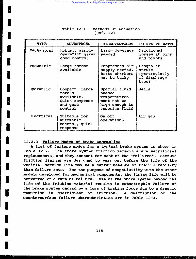
I

Table 12-1. Methods Of Actuation(Ref. 32)

UM

TYPE ADVANTAGES DISADVANTAGES POINTS 'O WATCHU Mechanical Robust, simple Large leverage Frictionaloperation gives needed losses at pinsgood control and pivots

Pneumatic Large forces Compressed air Length ofavailable supply needed. stroke

Brake chambers (particulai-lymay be bulky if diaphragm

type)

Hydraulic Compact. Large Special fluid Sealsforces needed.available. TemperaturesQuick response must not beand good high enough tocontrol vaporize fluid

I Electrical Suitable for On off Air gapautomatic operations• I Icontrol, quick

response Ick

1 12.2.3 Failure nodes of BrakejjgA list of failure modes for a typical brake system is shown in

Table 12-2. The brake system friction materials are sacrificia]replacements, and they account for most of the "failures". Becausefriction linings are designed to wear out before the life of the

I vehicle, service life may be a better measure of their durabilitythan failure rate. For the purpose of compatibility with the othermodels developed for mechanical components, the lining life will be3 converted to a rate of failure. Use of the brake system beyond thelife of the friction material results in catastrophic failure ofthe brake system caused by a loss of braking force due to a drasticreduction in coefficient of friction. A description of thecountersurface failure characteristics are in Table 12-3.

II3 149

I


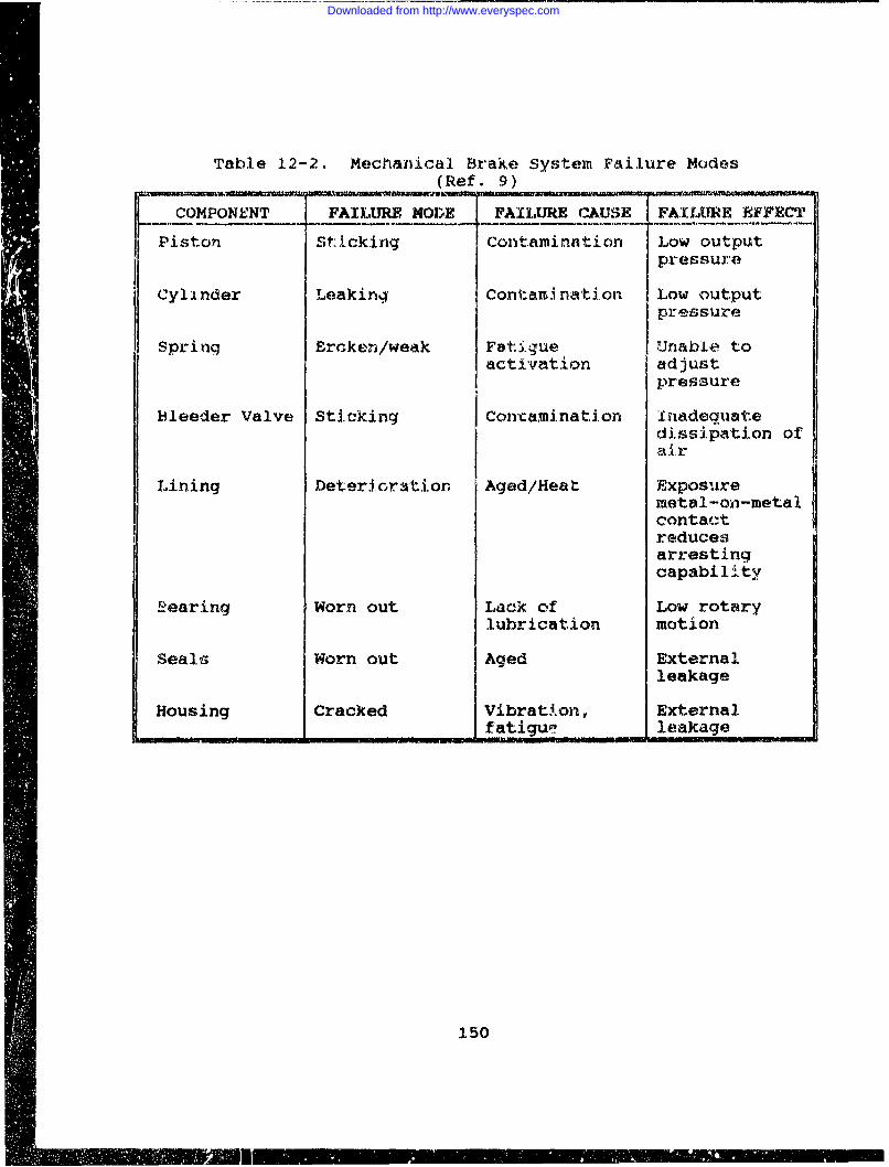
Table 12-2. Mechanical Br~ake System Failure Modes

COMPONENT FAILURE MOD~E FAILURE CAUSE FAILURE EFFECT

Piston Sticking Contaminaition Low outputpressure

Cyli~nder Leakin4 Contamni nation Low outputpressure

Sprinq Ercken/weak Fatigue Unable toactivation adjust

pressure

blieeder Valve Sticking Contamination Inadequatedissipation ofair

Lining fletericr~at~ion Aged/Heat Exposuremetal -on-metalcontactreducesarrestingcapability

R~earing Worn out Lack of Low rotarylubrication motion

Seals Worn out Aged Externalleakage

Housing Cracked IVibrati.on, External_______________~~~ __ ______ atigue lekag

150

=.:I


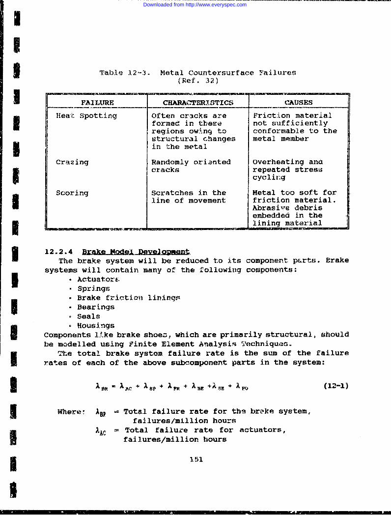
I

3 Table 122-3. Metal Countersurface Failures(Ref. 32)

FAILURE CHARACTERISTICS CAUSES

Heat Spotting Often cr3cks are Friction materialformed in these not sufficientlyregions owinq to conformable to thestructural changes metal member5 in the metal

Crazing Randomly oriented Overheating andcracks repeated stress

cycling

Scoring Scratches in the Metal too soft forline of movement friction material.

Abrasil'e debrisembedded in thelining material

I ~~12.2.4Brk de.The brake system will be reduced to its component p&rts. Brake

systems will contain many of the rollowing components:"" Actuatore;

"• Springs" Brake frictioii linings* Bearings" SealsHousings

Components 14.ke brake shoez, which are primarily structural, shouldbe modelled using finite Element Analysis Techniques.

The total brake system failure rate is the sum of the failurerates of each of the above subcomponent parts in the system:

A OR ACAc + SP + A' + Ak +*SzE + 1 (12-1)

w Where: Total failure rate for the broke system,fai.lures/million hours

XAC = Total failure rate for actuators,failures/million hours

151

I


Asp •Total failure rate for springs,failures/million hours

IF = Total !ailure rate for brake frictionmaterials, f'ailures/million hours

'XBE =Total failure rate for bearings,failures/mi ii ion hours

XSE - Total failure rate for seals,failare/million hours

AW = Total failure r:ate for brake housing, 3.0failures/million hours, from Navy Maintenanceand Material Management Information System

In the hydraulic drives of brake systems, seals are used toprevent leakage of brake fluid. The hardness and swelling of theseals, when exposed to brake fluid, must remain within limits suchthat the seals will give reliable operation. The reliability ofsprings associated with brake systemsi is generally very high whencompared to other components.

"Severe performance requirements may affect the reliability ofthe bearings if there is a path of heat conduction from thefriction surface to the bearings. This conduction may cause adecrease in the bearing lubricants operating viscosity and,consequently, a reduction in bearing life. A lubricant with ahigher temperature rating should prevent leakage or excessive wear.

The reliability of brake actuators normally is very high. Undersevere brake performance, conditions of increased temperature andexuessive vibration may decrease the reliability of thesecomponents. Refer to the appropriate sections of this Handbook forthe reliability models for individual parts comprising the brakeassembly. In some cases the result in failure/million cycles willhave to be converted to failures/million hours by multiplying bythe number of cycles per hour.

12.2.! toi iea1AAs stated in the introduction, the major functional components

of brake equipment and clutch equipment are the frictionmaterials. The reliability of brakes and clutches is concernedwith the wear of these friction materials. For brake assemblies,the friction lining provides the friction necessary to slow down orstop a vehicle. Friction materials used in clutches are placed inthe power-transmission system to couple it together so it rotatesas one unit.

152


3 Friction materials that are used in bra'ia and clutch liningshave severe performance requirements. The necessary energyconversion must be accomplished with a minimum of wear on thecontacting parts. For a particular type of brake or clutch, theamount of heat and friction generated varies according to 5conditions: (1) the amount of pressure applied between the slidingsurfaces, (2) the operating environment, (3) the roughness of thesurfaces, (4) the material from which the surfaces arn made, and3 (5) the frequency of application.

The reliability of these high energy components is important fora variety of reasons: Economy, operational readiness and, mostimportant, safety. In today's modern machinery and equipment, avast number of friction materials have become available to fulfillthe very diverse requirements of this equipment group. However, amaterial which is exceptional in all areas of friction materialcriteria does not yet exist.

In design it is necessary to have equations for the predictionI of the wear life of clutches and brakes. Lining wear properties aregenerally considered in terms of system life under several

' • different conditions of use severity. Consequently, lining life isoften the last performance character to be quantified. Thus aknowledge of lining wear behavior from laboratory testing can be of

11 great value.Friction modifier additives, such as cashew resin, graphite,

etc. have been used for many years in order to control frictionproperties in brake and clutch composites. Friction composites arecomposed of a balanced mixture of resin plus additives andgenerally contain over a dozen ingredients in order to achievedesired characteristics.

In the past, materials such as wood, leather and felt were used,but it was found that the usable temperature range was inadequateto cope with the ever increasing demands made upon them by theindustrial world. Today, friction materials can be divided intofive main groups:

1) Woven cotton2) Solid-woven asbestos3) Rigid molded asbestos, Semi-flex'.ble molded asbestos,

Flexible molded asbestos4) Sintered metal5) Cermets

Refer to Table 12-4 for a summary of friction material, types andapplications.

5 153

S


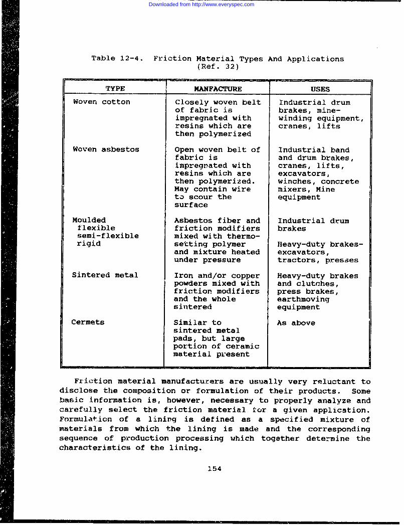
Table 12-4. Friction Material Types And Applications(Ref. 32)

TYPE I MANFACTURE USES

Woven cotton Closely woven belt Industrial drumof fabric is brakes, mine-impregnated with winding equipment,resins which are cranes, liftsthen polymerized

Woven asbestos Open woven belt of Industrial bandfabric is and drum brakes,impregnated with cranes, lifts,resins which are excavators,then polymerized. winches, concreteMay contain wire mixers, Mineto scour the equipmentsurface

Moulded Asbestos fiber and Industrial drumflexible friction modifiers brakessemi-flexible mixed with thermo-rigid setting polymer Heavy-duty brakes-

and mixture heated excavators,under pressure tractors, presses

Sintered metal Iron and/or copper Heavy-duty brakespowders mixed with and clutches,friction modifiers press brakes,and the whole earthmovingsintered equipment

Cermets Similar to As abovesintered metalpads, but largeportion of ceramicmaterial present

Friction material manufacturers are usually very reluctant todisclose the composition or formulation of their products. Somebasic information is, however, necessary to properly analyze andcarefully select the friction material kor a given application.Formulation of a lining is defined as a specified mixture ofmaterials from which the lining is made and the correspondingsequence of production processing which together determine thecharacteristics of the lining.

154


Organic linings are generally comprised of six basicingredients:

a) Asbestos for heat resistance and high coefficient offriction

b) Friction modifiers such as the oil of cashew nutshell togive desired friction qualities

c) Fillers such as rubber chips for controlling noised) Curing agents to produce the required chemical reactions in

the ingredientse) Materials such as powdered lead, brass chips, and aluminum

powders for improving the overall braking performancef) Binders such as phenolic resins for holding the ingredients

together

Organic linings designed for heavy-duty use generally havehigher inorganic contents to improve their high temperature wearresistance and fade resistance. Abrasives are generally added toachieve a higher friction coefficient.

Friction materials containing conventional organic bindingagents exhibit poor frictional stability under varying temperatureconditions. The thermal degradation of such binders results ininferior frictional characteristics, giving rise to fade and often

I resulting in increased wear. Furthermore, organic materials,particularly resins, tend to have a short shelf life, and are notalways easy to reproduce.U In an attempt to overcome the deleterious effects of poorthermal resistance in a friction material having an organic binder,various sintered metal and ceramic materiala, in which thesintering effects the bonding, have beert developed. ;n comparisonwith friction materials produced with organic, resinous bindingagents, sintered friction materials have the primary advantage ofbeing able to withstand considerably higher thermal stresses. Theyare produced from an intimate mixture of powdered metals andnonmetals by pressing and sintering.

Thesc friction materials commonly consist of sintered leadbronzes and iron powders with additions of dr7 lubricants andso-called friction reinforcers. Graphite and molybdenum sulfide,for example, are suitable as dry lubricants; on the other hand,ceramic additives and minerals, such as quartz and corunduu, may be3 used to increase the coefficient of friction. By appropriatevariation in the additives it is possible to make adaptations forI all applications, particularly as regards the coefficient offriction.

3 155


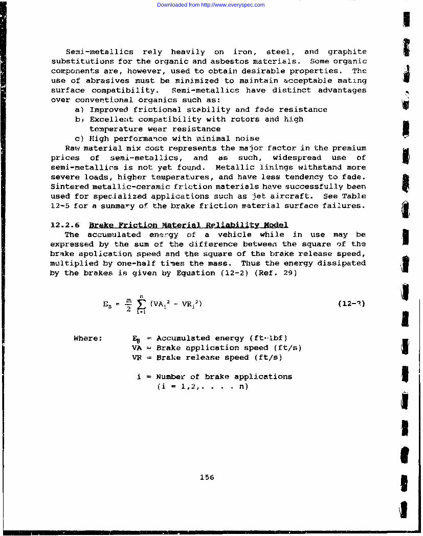
mU

Semi-metallics rely heavily on iron, steel, and graphitesubstitutions for the organic and asbestos materials. Some organiccomponents are, however, used to obtain desirable properties. Theuse of abrasives must be minimized to maintain &cceptable mating Nsurface compatibility. Semi-metallics have distinct advantagesover conventional organics such as:

a) Improved frictional stability and fade resistancebl Excellent compatibility with rotors and high

temperature wear resistancec) High performance with minnimal noise

Raw material mix cost represents the major factor in the premiumprices of semi-metallics, and as such, widespread use of Isemi-metallics is not yet found. Metallic linings withstand more

severe loads, higher temperatures, and have less tendency to fade.Sintered metallic-ceramic friction materials have successfully beenused for specialized applications such as jet aircraft. See Table12-5 for a summary of the brake friction vaterial surface failures.

12.2.6 DaeFito 4rA~iiiYi~The accumulated energy of a vehicle while in use may be

expressed by the sum of the difference between the square of thebrake application speed and the square of the brake release speed,multiplied by one-half times the mass. Thus the energy dissipated 3by the brakes is given by Equation (12-2) (Ref. 29)

EB (VAi 2 - VRi.2) (12-1)2 i -1 I

Where: ED = Accumulated energy (ft--lbf)VA = Brake application speed (ft/s)VR = Brake release speed (ft/s)

i = Number of brake applications 1(i = 1 ,. . .n)

156 3

I


S Table 12-5. Brake Friction Material Failure Modes(Ref. 32)

Problem Characteristics Causes

lHeat Spotting: Heavy gouging resulting in rapid Material rubbing againsk atlining wear heat-spotted metal member

Crazing: Randomly oriented cracks .r, Overheating of the brakingthe friction material, resulting in surf -- ea high wear rate

Scoring: Grooves formed on the friction Metal member needsmatera resulting in a reduct~on regrindingof life

Fade: Material degrades or flows at the Overheating caused byf'iction surface, resulting in a excessive brakingtemporary loss of performance

Metal Pick-Up: Metal from the mating member Unsuitable combination ofembedded in the lining materials

Grab: Lining contacting at ends only Incorrect radiusing of lininggiving high servo effect anderratic performance. rhe brakeis often noisy

Strip Braking: Braking over a small strip of Distortion of the brake paththe rubbing path givinglocalized heating and pre-ferential wear at those areas

Neglect: Material completely worn off Failure to provide anythe shoe giving a reduced maintenanceperformance

Misalignment' Excessive grooving and wear at Lining not iitted -orrectly 'opreferential areas of lining the shoe platformsurface

The heat equilibrium of the brake rotor in non-braking periods

I is shown by Equation 12-3 (Ref. 29).

1 157

I,


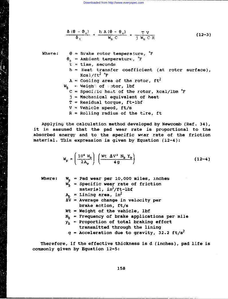
6 (e .- 00 h A(O - 8 ) T V

6t Wb C jWb C R

Where: 8 = Brake rotor temperasure, 0F00 Ambient. temperatures, OF

St time, secondsh= Heat transfer coefficient (at rotor surface),

Kca],/ft 2 OFA Cooling area of the rotor, ft 2

Wb Weigh' of .)tor, lbfC Speci'ic heat of the rotor, kcal/ibm OFj = Mechanical equivalent of heatT Residual torque, ft-lbfV = Vehicle speed, ft/sR = Rolling radius of the tire, ft

Applying the calculation method developed by Newcomb (Ref. 34),it is assumed that the pad wear rate is proportional to theabsorbed energy and to the specific wrar rate of the frictionmaterial. This expression is given by Equation (12-4):

04(io'Wb (Wt AV 2 Nb Yb) (12-4)2p A= j 4g

Where: Wp = Pad wear per 10,000 miles, i.nches

Wb = Specific wear rate of frictionmaterial, in 3/ft-lbf

Ap = Lining area, in 2

AV = Average change in velocity perbrake action, ft/s

Wt = Weight of the vehicle, lbfNb = Frequency of brake applications per mileyb - Proportion of total braking effort

transmitted through the liningg = Acceleration due to gravity, 32.2 ft/s 2

Therefore, if the effective thickness is d (inches), pad life iscommonly given by Equation 12-5:

158


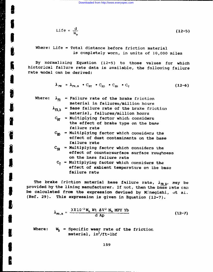
I

Life - d (12-5)Wp

Where: Life = Total distance before friction materialis completely worn, in units of 10,000 miles

By normalizing Equation (12-5) to those values for whichhistorical failure rate data is available, the following failurerate model can be derived:

AP = A,, * CB * CRO " 'Sr * CT (12-6)

Where: IFR = Failure rate of the brake frictionmaterial in failures/million hours*kF, = Base failure rate of the brake frictionmaterial, failures/million hours

CBT Multiplying factor which considersI the effect of brake type on the basefailure rate

CR= Multiplying factor which considers theeffect of dust contaminants on the basefailure rate

C = Multiplying factor which considers theeffect of countersurface surface roughnesson the base failure rate

C Multiplying factor which considers theeffect of ambient temperature on the basefailure rate

The brake .riction material base failure rate, XRB, may beprovided by the lining manufacturer. If not, then the base rate canbe calculated from the expression devised by H-negishi, ot al.(Ref. 29). This expression is given in Equation (12-7).

3 3X1O-3 Wb Wt AV2 Nb MPY Yb

,B = d Ap

Where: Wb = Specific wear rate of the frictionI material, in3/ft-lbf

159

,sI


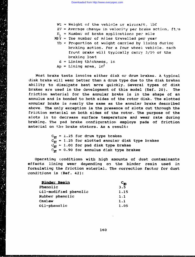
Wt - Weight of the vehicle or aircr&ft., IbfAV - Aver:age change in velocity per brdko action, ft/sNb = Number of brake applicntior.n per mile

"MPY =Tne number of rnJles travelled per yearYb : Proportion o0 weight carried by linlirng durinq

braking action. For a four wheel vehicle, eaIhfrunt brake will typically carry, 3/1() of thebraking load

d = Lining thJ. ckness, in

Ap Lining area, in2

Most brake tests involve either disk. or drum brakes. A typicaldisk brake will wear better than a drum type due to the disk brakesability to dissipate heat more quickly. Several types of diskbrakes are used in the development of this model (Ref. 20). The.friction material for the annular brake is in the shape of anannulus and is bonded to both sides of the rotor disk. The slottedannular brake is nearly the same as the annular brake describedabove. The only e:ception is the presence of slots cut through thefriztion material on both sides of the rotor. The purpose of theslots is to decrease surface temperature and wear rate duringbraking. The pad brake configuration employs pads of frictionmatev-ial on the brake stators. As a result:

SC7 B -1.25 for drum type brakesC BT = 25 for slotted annular disk type brakesC BT - 1.00 for pad disk type brakes(IST = 0.90 for annulus disk type brakes

Operating conditions with high amounts of dust contaminantseffects lining wear depending on the binder resin used informulating the friction material. The correction factor for dustconditions is (Ref. 42):

BindOaLResin CIPhenolic 3.5oil-modified phenolic 1.15Rubber phenclic 1.1Cashew 1.1Oil-phenolic 1.05

160


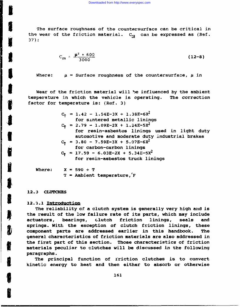
Si The surface roughness of the countersurface can be critical inthi wear of the friction material. c,, can be expressed as (Ref.37):

ICSR 2 + 600 (12-8)"sR = 3000

5 Where: = Surface roughness of the countersurface, p in

I Wear of the friction material will ble influenced by the ambienttemperature in which the vehicle is operating. The correctionfactor for temperature is: (Ref. 3)

CT = 1.42 - 1.54E-3X + 1.38E-6X2

for sintered metallic liningsCT = 2.79 - 1.09E-2X + 1.24E-5X2

for resin-asbestos linings used in light dutySautomotive and moderate duty industrial brakes

CT = 3.80 - 7.59E-3X + 5.07E-6X2

for carbon-carbon liningsCT = 17.59 - 6.03E-2X + 5.34E-5X2

for resin-asbestos truck linings

K Where: X = 590 + T

T = Ambient temperature,O'F

12.3 CLUTCHES

S 12.3.1 IntrpdU~fjg

The reliability of a clutch system is generally very high and isthe result of the low failure rate of its parts, which may includeactuators, bearings, clutch friction linings, seals andsprings. With the exception of clutch friction linings, thesecomponent parts are addressed earlier in this handbook. Thegeneral characteristics of friction materials are also addressed in

ft the first part of this section. Those characteristics of frictionmaterials peculiar to clutches will be discussed in the followingparagraphs.

The principal function of friction clutches is to convertkinetic energy to heat and then either to absorb or otherwise

5 161

S


dissipate the heat while simultaneously, through friction, reducingthe relative movement between the friction material and the part towhich it is engaged. In order to achieve these objectives thenecessary energy conversion must be accomplished with a minimum ofwear on the contacting parts.

12.3.2 Clutch VarietiesClutches are made up of two basic components -- the pressure

plate and disc. The pressure plate supplies sufficient force orpressure to the disc so enough friction is developed to transmittorque to the driveline.

Friction clutches, although available in many different formstend to be of the axial or rim type. Axial clutches operate wherethe movement is parallel to the axis of the shaft. Rim typesoperate where the movement is radial. examples of the former arethe plate and cone clutches. Examples of the latter include coil orwrap spring and chain clutches.

Plate clutches divide into two designs - single andmultiplate. The single plate design is the type favored byautomotive designers for transmission and light to medium powerapplications. The single plate is normally provided with a frictionlining on each side of the disc. Multiplate designs employ a numberof discs lined on both sides which serve to distribute the loadover a large area. These types are used for high torque and highload applications. They required only moderate clamping pressures,and are suitable for high speed operation because their relativelysmall size generates lower centrifugal forces.

Cone clutches are used for smaller, medium power, low speedtransmission systems which may be subjected to rough usage. Thesedevices cope well with such treatment because of their simplerobust construction, and due to the fact that heat is dissipatedmore readily than with plate clutches.

Rim and block clutches employ various means of engaging thestationary half of the assembly through radial movement against therim of the driving member. The action is similar to that of aninternally expanding brake shoe.

Centrifugal clutches are often used with squirrel cagemotors. The fabric facing may be fitted to shoes or blocks mountedto a spider which is keyed onto the driving shaft. The shoes orblocks are thrown outward by centrifugal force, engagement beingautomatic when a predetermined speed is reached from starting.

Coil or wrap spring clutches operate on the principle of aspring mounted on a drum being tightened. The action is much like

162


I

5 that of a rope tightening around a revolving capstan. The design iscompact, simple in construction and is used where high torques ar-erequired from low power. For this reason the clutches have foundapplications in small equipment such as plain paper copiers and, intheir larger versions, for haulage gears and rolling mills andpresses.

Chain clutches employ inner and outer friction rings in an oilfilled housing actuated by cams bearing on chain toggles whichforce the rings together.

Sprag clitches consist of a number of specially shaped steelsprings or wedges which jam inner and outer races in one directiononly. This action leads to their use for applications inover-running (where the clutch acts as a free-whseel) andback-stopping. This design is particularly useful for intermittentrotary motion involving, for example, inuexing or inching (Ref. 34)

Materials c!assificaticn divides the friction materials intoorganic and metallic groups. The organic group includes allmaterials composed ot both asbestos and non-asbesto3 fibers andbound by some resin binder. The metallic group consists of allfriction materials containing iron, copper, ceramic brcnze,graphite, carbon or other metallic material such as the basematerial.

12.3.3 Clutch Model •eeopmen;The clutch system reliabili.. model will contain the followingI component parts:

• Actuators• Bearings• Clutch friction linings. Sealsi Springs

The total clutch system failure rate is the sum of the failure3 rates of each of the above subcomponent parts in the system:

A. CL I AC + IBE + X CF + I SE + X SP (12-9)

Where: X= Total failure rate for the clutchsystem, failures/million hours

AAC = Total failure rate for actuators,failures/million hours

1! 163

I


IBE Total failure rate for bearings,failures/million hours

XCF Total failure rate for clutch frictionmaterials, failures/million hours

SE- Total faiiure rate for seals,f-faJlures/million hours

I= Total failure rate for springs,failures/million hours

R-efer to Chapter 3 of this Handbook for a description of theseal reliability model. Note that the failure rate obtained mustbe converted from failures/million cycles to failures/million hoursby multiplying by the number of cycles per hour. Failure ratemodels for springs, bearings, and actuators are given in Chapters4, 7, and 9 respectively. Again, note that the results from thesesactions must be converted to failures/million hours. The failurerate model for clutch friction materials is presented in thefollowing paragraphs.

12.3.4 Q~bh riction Nateral Reliability &nelA list of failure modes for a clutch friction materials is shown

in Table 12-6. Use of the clutch system beyond the life of thefriction material results in catastrophic failure of the clutchcaused by a drastic reduction in coefficient of friction.

Under normal operating conditions, the friction materials usedin clutches are reliable mechanical components. Like brake frictionmaterials, the wear of clutch materials is dependent on the amountof accumulated energy dissipated by the mechanical component. Therating of the clutch friction material, R, is given in Equation(12-11) per Ref 16.

RC (12--11)550 t AC

Where: R - Rating of friction materials, h.p./in2

EC = Average energy dissipated perapplication, ft-blf.

t = Slipping time, sec.Ac - Area of clutch friction material, in 2

164


The life of the friction material, L, is given by Equlation(12-.12): (Ref. 12)

3600d WV (12-12)

Where: L - Life of clutch friction material, hoursSd = Effective thickness of lining , inches

WV = Average wear value of the material,h.p.-hr/in

3

n = Number of applications per hour3.

The average wear valve, WV, should be supplied by the fzictionmaterial manufacturer for each material type. Combining Equationg (12-11) with Equation (12-12) yields:

2X106 d WVAC (12-13)ft Ecn

The clutch friction material base failure rate, AIC, may besupplied by the clutch lining manufacturer. The base failure rate

I can also be calculated from Equation (12-13) as:

I ECn (12-14)i! cF'B- 2dWVAC

Where: CFB= Base failure rate of the clutch friction

matarial in failures/mill.ion hours.

By normalizing Equation (12-14) to those values for which

historical failure rate data is available, the followlng failure5 rate model can be derived:

A CF= ACF,B 0 CNP CT (12-15)

5 Where: C• = Multiplying factor which considers

1I 165

I


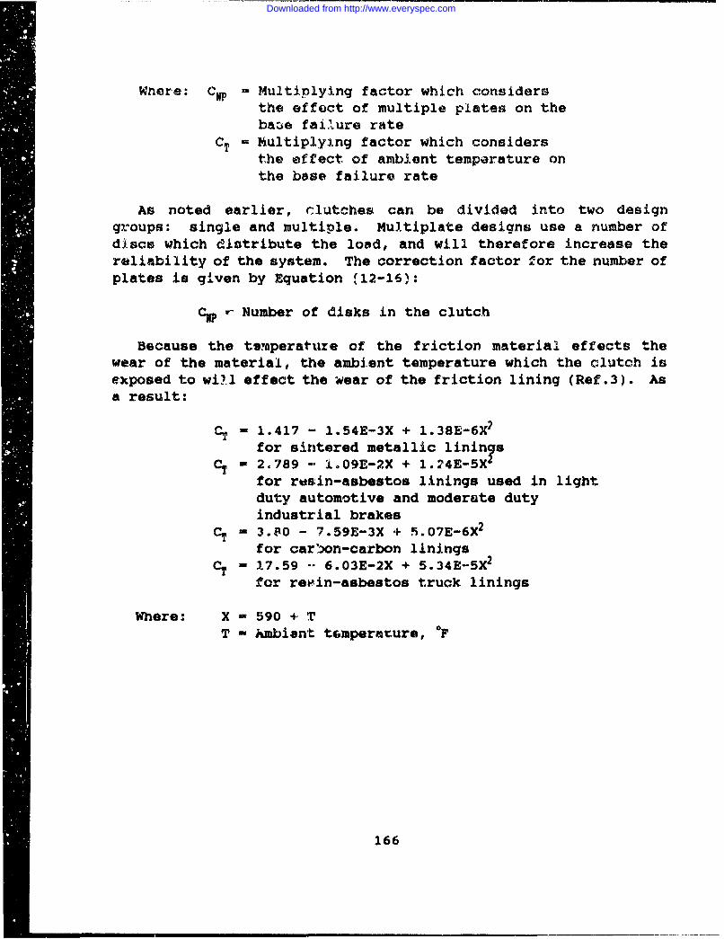
Wnere: CP - Multiplying factor which considersthe effect of multiple plates on thebase failure rate

CT = Multiplying factor which considersthe effect of ambient temperature onthe base failure rate

As noted earlier, clutches can be divided into two designgroups: single and multiple. Multiplate designs use a number ofdiscs which distribute the load, and will therefore increase thereliability of the system. The correction factor for the number ofplates is given by Equation .12-16):

C• - Number of disks in the clutch

Because the temperature of the friction material effects thewear of the material, the ambient temperature which the clutch isekposed to will effect the wear of the friction lining (Ref.3). Asa result:

S- 1.417 - 1.54E-3X + 1.38E-6X2

for sintered metallic lininsCT - 2.789 -- 1.09E-2X + 1.24E-5X

for rusin-asbestos linings used in lightduty automotive and moderate dutyindustrial brakes

CT - 3.80 - 7.59E-3X + 5.07E-6X2

for carbon-carbon liningsCT - 17.59 -- 6.03E-2X + 5.34E-5X2

for revin-asbestos truck linings

Where: X - 590 + TT - Ambiant t~mperarure, *F

166


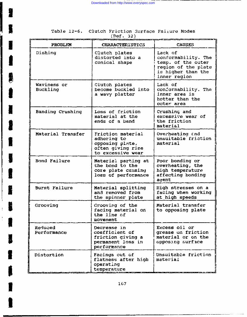
i I Table 12-6. Clutch Friction Surface Faij.u1e Modes(Ref. 32)

i_ PROBLKM CHARACTERXSTICS CAUSES

Dishing Clutch plates Lack ofdistorted into a conformability. Theconical shape temp. of the outer

Sregion of the plateis higher than theinner region

Waviness or Clutch plates Lack ofBuckling become buckled into conformability. The

a wavy platter inner area ishotter than the

outer area

Banding Crushing Loss of friction Crushing andmaterial at the excessive wear ofends of a band the friction

material

Material Transfer Friction material Overheating c.nd3 adhering to unsuitable frictionopposing plite, materialoften giving riseto excessive wear

Bond Failure Material parting at Poor bonding orthe bond to the overheating, thecore plate causing high temperatureloss of performance affecting bonding

agent

Burst Failure Material splitting High stresses on aand removed from facing when workinqthe spinner plate at high speeds

Grooving Grooving of the Material transferfacing material on to opposing platethe line cfI�-movement

Reduced Decrease in Excess oil orPerformance coefficient of grease on friction

friction giving a material or on thepermanent loss in opposing surfaceperformance

3 Distortion Facings out of Unsuitable frictionflatness after high materialoperatingtemperature

3 167

I



168


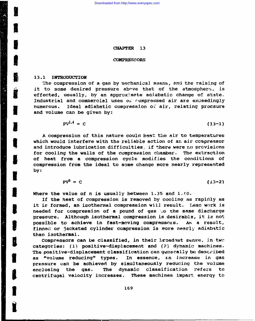
StCHAPTER 13

3 COMPRESSORS

I 13.1 INTRODUCTIONThe compression of a gas by mechanical means, and the raising of

it to some desired pressure abr've that of the atmosphere, iseffected, usually, by an approxAimate adiabatic change of state.Industrial and comnercial uses o. r•ompressed air are exceedinglynumerous. Ideal adiabatic compression oi air, relating proesureand volume can be given by:

1 PV1'4 = C (13-1)

A compression of this nature could heat the air to temperatures3 which would interfere with the reliable action of an air compressorand introduce lubrication difficulties, if there were no provisionsfor cooling the walls of the compression chamber. The extractionof heat from a compression cycle modifies the conditions ofcompression from the ideal to some change more nearly representedSI by:

PV1 = C (13-2)

I Where the value of n is usually between 1.35 and .lO.If the heat of compression is removed by cooling as rapidly as

it is formed, an isothermal compression will result. Less work isI needed for compression of a pound of gas %o the same dischargepressure. Although isothermal compression is desirable, it is notpossible to achieve in fast-moving compressors. As a result,finned or jacketed cylinder compression is more nearly adiabaticthan isothermal.

Compressors can be classified, in their broadast sense, in twc'categories: (1) positive-displacement and (2) dynamic machines.The positive-displacement classification can generallyy be describedas "volume reducing" types. In essence, am increase in gaspressure can be achieved by simultaneously reducing the volumeenclosing the gas. The dynamic classification refers tocentrifugal velocity increases. These machines impart energy to

3169


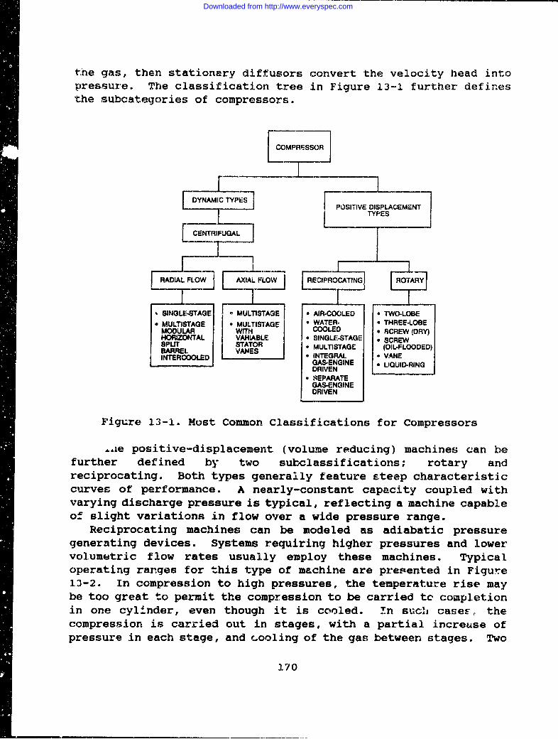
the gas, then stationary diffusors convert the velocity head intopressure. The classification tree in Figure 13-1 further definesthe subcategories of compressors.

LCOMPRESSOR

[DYNAMIC TYPE~S FPOSITVE DISPLACEMENT7

I TYPESCENTRIFUGAL

RADIAL FLOW AXIAL FLOW REROTARY

SINGLE-STAGE e MULTISTAGE a AIR-COOLED * TWO-LOBEMULTISTAGE * MULTISTAGE * WATER- * THREE-LOBEMODULAR WITH COOLED e SCREW (DRY)HORIZONTALI VARIABLE * SINGLE-STAGE * SCREWSPLU STATOR * MULTISTAGE (OIL-FLOODED)BARREL VANESINTERCOOLED a INTEGRAL - VANE

GAS-ENGINE - UQUID-RINGDRIVEN

* SEPARATEGAS-ENGINEDRIVEN

Figure 13-1. Most Common Classifications for Compressors

,ae positive-displacement (volume reducing) machines can befurther defined by two subclassifications; rotary andreciprocating. Both types generally feature steep characteristiccurves of performance. A nearly-constant capacity coupled withvarying discharge pressure is typical, reflecting a machine capableof slight variations in flow over a wide pressure range.

Reciprocating machines can be modeled as adiabatic pressuregenerating devices. Systems requiring higher pressures and lowervolumetric flow rates usually employ these machines. Typicaloperating rarges for this type of machine are presented in Figure13-2. In compression to high pressures, the temperature rise maybe too great to permit the compression to be carried tc completionin one cylinder, even though it is cooled. in such case,, thecompression is carried out in stages, with a partial increase ofpressure in each stage, and cooling of the gas between stages. Two

170


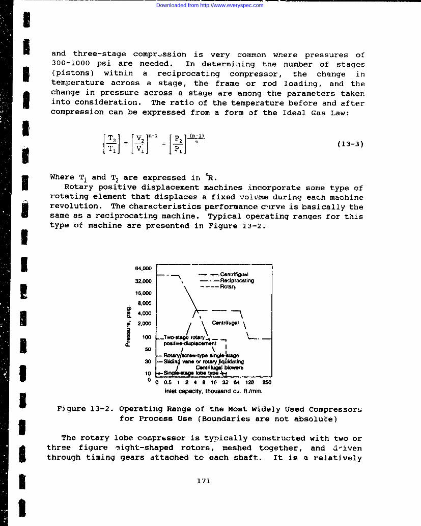
SI and three-stage compr.ession is very common where pressures of300-1000 psi are needed. In determining the number of stages

SI (pistons) within a reciprocating compressor, the change intemperature across a stage, the frame or rod loading, and theE• change in pressure across a stage are among the parameters takeninto consideration. The ratio of the temperature before and aftercompression can be expressed from a form of the Ideal Gas Law:

S[V L (13-3)-VWhere T1 and T2 are expressed in 0R.

Rotary positive displacement machines incorporate some type ofrotating element that displaces a fixed volume during each machine

i revolution. The characteristics performance curve is basically thesame as a reciprocating machine. Typical operating ranges for thistype of machine are presented in Figure 13-2.

*- 8 4,000

64. 0-. Centtifigtial

32,000 _ - - -Reciprocatingo .... Rotar)I 15,000

8,000

4,000 -

S2.000 / \Centrfugl100 -Two-tago rotary,. -

(. powtive-displ-acment

-Fotq/screwtype snQi8QS30 -lidig va* orrotary )qcli~datng

Ce' cntrifugal blowers10 ,- SIN$.tage lobe type - .0 0 0.5 1 2 4 8 18 32 64 128 250

Inlet capacity, thousand cu. ft./min.

S Figure 13-2. Operating Range of the Most Widely Used Compressorsifor Process Use (Boundaries are not absolute)

The rotary lobe cozprussor is typically constructed with two orI three figure .ight-shaped rotors, meshed together, and 4-iventhrough timing gears attached to each shaft. It is a relatively

3 I171


low pressure machine (5 to 7 psig, and up to 25 psig for specialtypes) and is well suited for applications with vacuum pressures.Its performance is notable for a greater throughput capability,with little or no flow pulsation.

The rotary screw compressor yields considerably higher pressuresand speed. Again, its performance is characteristic of a greaterthroughput capability with little or no pulsation.

The sliding vane rotary compressor has a rotor constructionwhich is offset, containing slots for vanes to slide in and outduring each revolution. These vanes gradually reduce the volume ofa trapped gas, raising its pressure. This machine is used forrelatively low pressure operations (up to 50 psig per stage).

A liquid ring (or piston) rotary is constructed of circularvanes, turning inside a casing sealed with a liquid. Centrifugalforces cause the liquid to form a ring around the periphery of thecasing interior, while forcing the gas inward toward the center ofthe vaned rotor. The gradual decrease in volume increases thepressure of the gas. Any liquid entrained in the gas is separatedout. This type of machine is characteristically used in lowpressure and vacuum applications.

Centrifugal compressors can be divided into two subcategoriesbased on the direction of flow of the product gas: radial flow andaxial flow machines. The characteristic curves of these machinesoffer a wide range in flow with a corresponding small change inhead. Flow is smooth and pulsation-free beyond the surga point onth3 performance curve. The lack of rubbing parts in the compressedgas stream is a particularly desirable feature of these machinesfrom a designer's standpoint.

In radial compressors, velocity is imparted to a gas streamthrough centrifugal forces acting in a radial direction to theshaft. The simplest style of radial centrifugal compressor is thesingle-stage overhung design. The conventional closed or shroudedimpeller is used for adiabatic heads to about 12,000 tt-lb/lb. Theopen, radial-bladed impeller develops more head for the samediameter and speed.

In axial flow machines, the gas flow remains parallel to theshaft, without a direction change. These machines are typicallyused for higher capacities than radial flow machines, but generatemuch lower head per stage. As a result, these machines are usuallybuilt with many stages. The characteristic performance curve issteeper then the radial flow machines, with a more narrow stabilityrange.

172


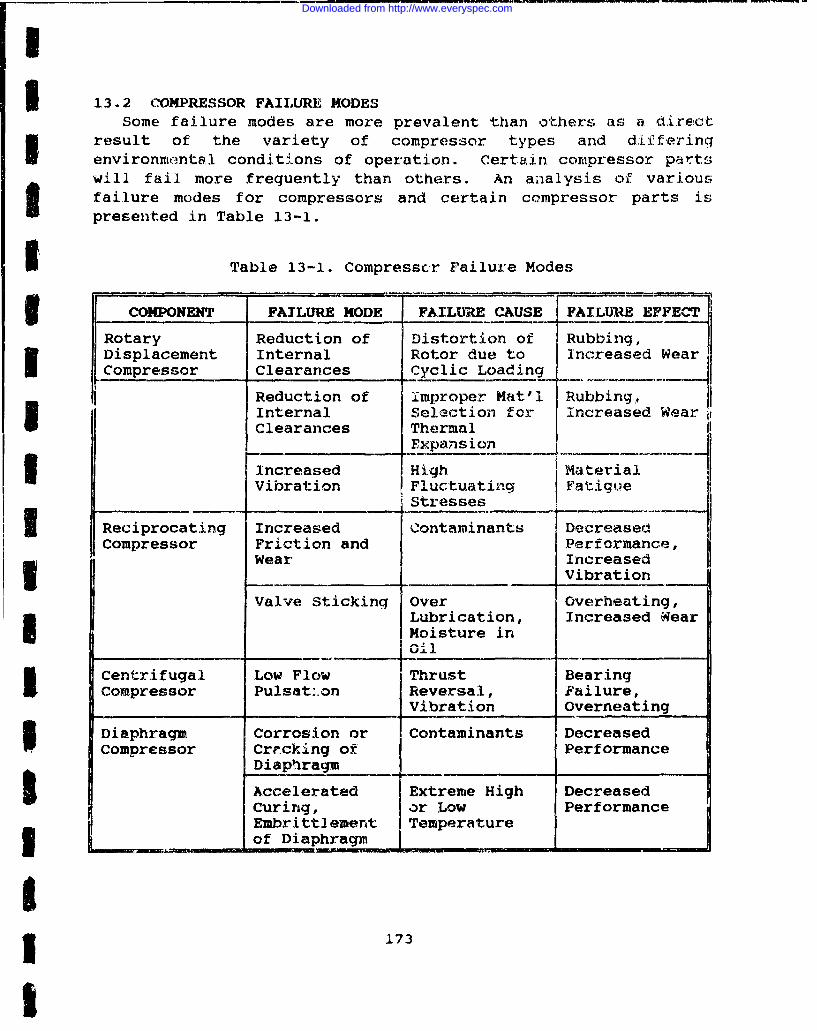
13.2 COMPRESSOR FAILURE MODESSome failure modes are more prevalent than others as a (irect

result of the variety of compressor types and dixfferingenvironmental conditions of operation. Certain compressor partswill fail, more frequently than others. An analysis of variousfailure modes for compressors and certain compressor parts ispresented in Table 13-1.

SI Table 13-1. Compresscr Failure Modes

COMPONENT FAILURE MODE FAILURE CAUSE FAILUREEFFECT

Rotary Reduction of Distortion of Rubbing,Displacement Internal Rotor due to Increased WearCompressor Clearances Cyclic Loading

Reduction of improper Mat'l Rubbing,Internal Selection for Increased WearClearances Thermal

ExpansionIncreased High MaterialVibration Fluctuating Fatigue

Stresses

I Reciprocating Increased Contaminants DecreasedCompressor Friction and Performance,

Wear IncreasedVibration

Valve Sticking Over Overheating,Lubrication, Increased WearMoisture in

______ ~Oil _ _ _ _

* Centrifugal Low Flow Thrust BearingCompressor Pulsati..on Reversal, Failure,

Vibration Overneating

Diaphragm Corrosion or Contaminants DecreasedCompressor Crocking of Performance

Diaphragm

Accelerated Extreme High DecreasedCuring, or Low PerformanceEmbrittlement Temperatureof Diaphragm

3 173

I


.13.3 MODEL DEVEIlDPHiINT

Any compressor, taken as a complete operating system, can bereduced to the following series of models of each of itssubcomponent parts. Each of these parts will sum to the totalcompressor failtire rate:

1 1A SH + 3! + ACA + AVA + ISE + AD (13-4)

W1here: Ac Total failure rate of compressor,

failures/million cyclesTotal failure rate for the compressorshaft(s), failures/million cycles,see Chapter 10

XBE = Total failure rate for all compressorbearings, failures/million cycles,see Chapter 7

I = Total failure rate for the compressorcasing, failures/million cycles,see Section 13-4

AVA = Total failure rate for any valve assembly,failures/million cycles, see Chapter 6

ISE = Total failure rate for all compressor seals,failures/million cycles, see Chapter 3

-k• = Total failure rate due to designconfiguration, failures/million cycles,see Section 13-5

The failure rate, A, for each part listed above must be known orcalculated before the entire system failure rate, XC, can bedetermined. Values of each part A will incorporate expectedoperational and environmental factors that exist during normalcompressor operation.

13.4 FAILURE RATE MODEL FOR Q12SINGThe compressor casing, normally a very reliable component, can

have a large effect on the life of other components in thecompressor assembly (especially seals and bearings). The value ofreliability of compressor casings, through the experience of manydifferent manufacturers, can generally be equated to as high avalue as 10-4 failures/million cycles.

174


I

3 13.5 FAILURE RATE MODEL FOR COMPRESSOR DESIGN CONFIGURATIONVarious reliabilities are inherent in specific designs (types)

of compressors. For example, it is expected that reliability dueto weir will be different in a rotary screw compressor compared toa centrifugal compressor due to the nature of metal-to-metalcontact and rotor speeds.

In its broadest sense, the parameter AD, can be approximated bydata presented in Table 10-3 for various types of fluid drivers,developed from information collected by the U.S. Navy. This datawill suffice in the absence of a complete development of eachspecific type of compressor presented in Figure 13-1. As new, morespecific models are added A can be replaced with the individualmodel. For Example:

5• = )'DI

Where: A = Total failure rate of the configurationdiaphragm compressor

U 13-6 FAILURE RATE MODEL FOR COMPRESSOR DIAPHRAGMSThe configuration diaphragm compressor failure rate model can be

described by:

ADI AB Cp CAC LC CSF CT (13-5)

SWhere: ABFD Compressor diaphragm base failure rate,0.40 to 0.75 failures/million hrs.

CP = Factor for effects of load variation(performance), see Set;'ion 13.6.1CAC = Factor for effects of atmospheric

contaminants, see Section 13.6.2C = Factor for effects of liquid

contaminants, see Section 13.6.3CSF = Factor effects of surface finish

or coatings, see Section 13.6.4C= Factor for effects of temperature,

S see Section 13.6.5

Diaphragms, in general, are round flexible plates which undergo3 an elastic deflection when subjected to an axial loading. In theapplication of compressors, this axial loading and elasticdeflection creates a reduction in volume of the space adjacent tothe diaphragm. The gas is compressed and a pressure builds. The

3 175

I


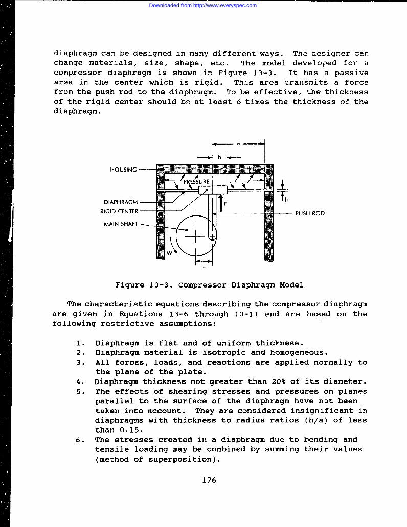
diaphragm can be designed in many different ways. The designer canchange materials, size, shape, etc. The model developed for acompressor diaphragm is shown in Figure 13-3. It has a passivearea in the center which is rigid. This area transmits a forcefrom the push rod to the diaphragm. To be effective, the thicknessof the rigid center should beý at least 6 times the thickness of thediaphragm.

a-

HOUSING SPRESSURE'

DIAPHRAGM F Ih

RIGID CENTER PUSH ROD

MAIN SHAI ..-.-T

Figure 13-3. Compressor Diaphragm Model

The characteristic equations describing the compressor diaphragmare given in Equations 13-6 through 13-11 and are based on thefollowing restrictive assumptions:

1. Diaphragm is flat and of uniform thickness.2. Diaphragm material is isotropic and homogeneous.3. All forces, loads, and reactions are applied normally to

the plane of the plate.4. Diaphragm thickness not greater than 20% of its diameter.5. The effects of shearing stresses and pressures on planes

parallel to the surface of the diaphragm have nDt beentaken into account. They are considered insignificant indiaphragms with thickness to radius ratios (h/a) of lessthan 0.15.

6. The stresses created in a diaphragm due to bending andtensile loading may be combined by summing their values(method of superposition).

176


I

5 The characteristic equation of a rigid center diaphragm loadedby a force for any magnitude of deflection is given by EquationE (13-6). It is applicable for (b/e) ratios greater than 0.05°

I. F- E [hya2 ÷hyo3Bj (1--6)

Where: F = Force applied to rigid disk ofdiaphragin, lbs.

E = Modulus of elasticity, psia = Radius of diaphragm, inh = Diaphragm thickness, in

YI = Vertical deflection at center ofdiaphragm, in

KF = Modified Stiffness Coefficient based ondiaphragm bending loads,

=3 (1 - g2) c L l{ 1.3-7)4c 2 c 2 - 1

3 B = Stiffness coefficient based on diaphragritensile loading, as follows:

7 - I ' +b2 -b+ + [(3-1)2J b 2

3 \ a_ _a_ _ ' [1 + 1!1 a 2

3 (1-0) L-

p = Poisson~s ratioc = Ratio of radii (diaphragm-to-disk),

a/b, in/in5 b = Radius of rigid center plate of diaphragm, in

The maximum radial stress for a f o.-ce- loaded diaphragm withI rigid center occurs at the inner perimeter of the diaphragm (b).

a h2xoU (13-S,KFBF

3 177

I


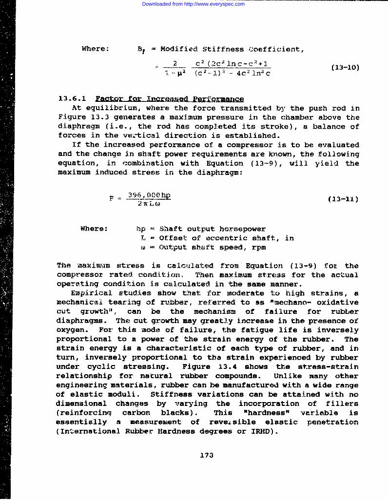
Where: BF Modified Stiffness Coefficient,

2 c 2 (2c 2 Inc-c+3. (13-10)

. -. p2 (C 2_ )2 - 4c2In 2 c

13.6.1 Fact msieQnrI oaVmnAt equilibrium, where the force transmitted by the push rod in

Figure 13.3 generates a maximum pressure in the chamber above thediaphragm (i.e., the rod has completed its stroke), a balance offorces in the ve.tical direction is established.

If the increased performance of a compressor is to be evaluatedand the change in shaft power requirements are known, the followingequation, in combination with Equation (13-9), will yield themaximum induced stress in the diaphragm:

F =3 ,ooh0p (2.3-li)2 w Lcto

Where: hp Shaft output horsepowerSL Offset of eccentric shaft, inw Output shaft speed, rpm

The maximum stress is calculated from Equation (13-9) for thecompressor rated condition. Then maximum stress for the actualoperating condition is calculated in the same manner.

Empirical studies show that for moderate to high strains, amechanical tearzing of rubber, referred to as "mechano- oxidativecut growth•,' can be the mechanism of failure for rubberdiaphragms. The cut growth may greatly increase in the presence ofoxygen. For this mode of failure, the fatigue life is inverselyproportional to a power of the strain energy of the rubber. Thestrain energy is a characteristic of each type of rubber, and inturn, inversely proportional to the strain experienced by rubberunder cyclic stressing. Figure 13.4 shows the stress-strainrelationship for natural rubber compounds. Unlike many otherengineering materials, rubber can be manufactured with a wide rangeof elastic moduli. Stiffness variations can be attained with nodimensional changes by varying the incorporation of fillers(reinforcinq carbon blacks). This "hardness" variable isessentially a measurement of reveisible elastic penetration(International Rubber Hardness degrees or IRHD).

173


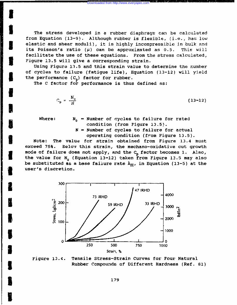
I

i The stress developed in a rubber diaphragq carl be calculatedfrom Equation (13-9). Although rubber is flexible, (i.e., has lowI elastic and shear moduli), it is highly incompressible. in bulk andits Poisson's ratio (p) can be approximated as 0.5. This willfacilitate the use of these equations. From the stress calculated,3 Figure 13.5 will give a corresponding strain.

Using Figure 13.5 and this strain value to determine the numiberI of cycles to failure (fatigue life), Equation (13-12) will yieldthe performance (CP) factor for rubber.

The C factor for performance is thus defined as:

IC N-N (13-12)INWhere: No = Number of cycles to failure for rated

I condition (from Figure 13.5).N = Number of cycles to failure for actual

operating condition (from Figure 13.5).U Note: The value for strain obtained from Figure 13.4 mustexceed 75%. Below this strain, the mechano-oxidative cut growthmode of failure does not apply, and the C factor becomes 1. Also,the value for No (Equation 13-12) taken from Figure 13.5 may alsobe substituted as a base failure rate ADI, in Equation (13-5) at the

SI user's discretion.

I ~3000 147 IRHD

73 IRHD 400N ~E 200 " 3I-

U 59 IRHD 33IRHD

2000 --

VI 1V -0 000

250 500 750 1000Strain, %

Figure 13.4. Tensile Stress-Strain Curves for Four Natural3 Rubber Compounds of Different Hardness (Ref. 81)

5 179

I


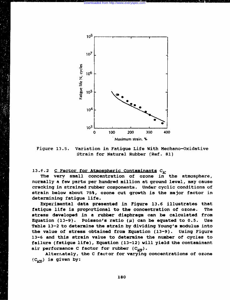
108

1 07

ii S~106

.29 105 \ _

U... --104.-io

0 100 200 300 400

Maximum strain, %

Figure 13.5. Variation in Fatigue Life With Mechano-Oxidative-Strain for Natural Rubber (Ref. 81)

13.6.2 C Factor for Atmospheric Contaminants CACThe very small concentration of ozone in the atmosphere,

normally a few parts per hundred million at ground level, may causecracking in strained rubber components. Under cyclic conditions ofstrain below about 75%, ozone cut growth is the major factor indetermining fatigue life.

Experimental data presented in Figure 13.6 illustrates thatfatigue life is proportional to the concentration of ozone. Thestress developed in a rubber diaphragm can be calculated fromEquation (13-9). Poisson's ratio (p) can be equated to 0.5. UseTable 13-2 to determine the strain by dividing Young's modulus intothe value of stress obtained from Equation (13-9). Using Figure13-6 and this strain value to determine the number of cycles tofailure (fatigue life), Equation (13-12) will yield the contaminantair performance C factor for rubber (CAI).

Alterrately, the C factor for varying concentrations of ozone(CIO) is given by:

180


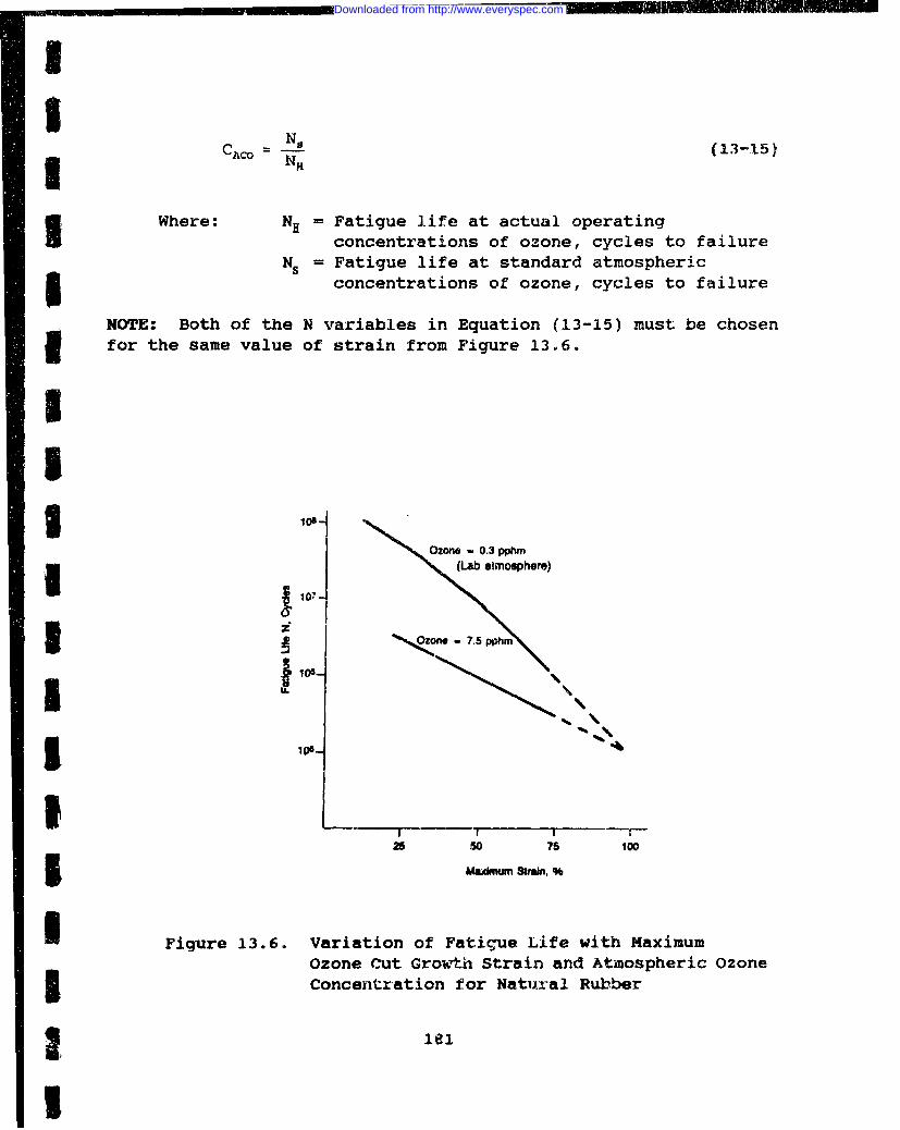
.I'

CAO-No (13-15)

Where: Na = Fatigue life at actual operatingconcentrations of ozone, cycles to failure

Ns = Fatigue life at standard atmospheric5concentrations of ozone, cycles to failure

I] NOTE: Both of the N variables in Equation (13-15) must be chosenfor the same value of strain from Figure 13.6.

II

Ozone - 0.3 ppem

I (Lab atmosphere)

Sne - 7.5 m'h

[] I U-

i 10-

2I so 75 17

5 Maamum Strain. %

U Figure 13.6. Variation of Fatigue Life with MaximumOzone Cut Growtih Strain and Atmospheric OzoneConcentration for Natural Rubber

181

I


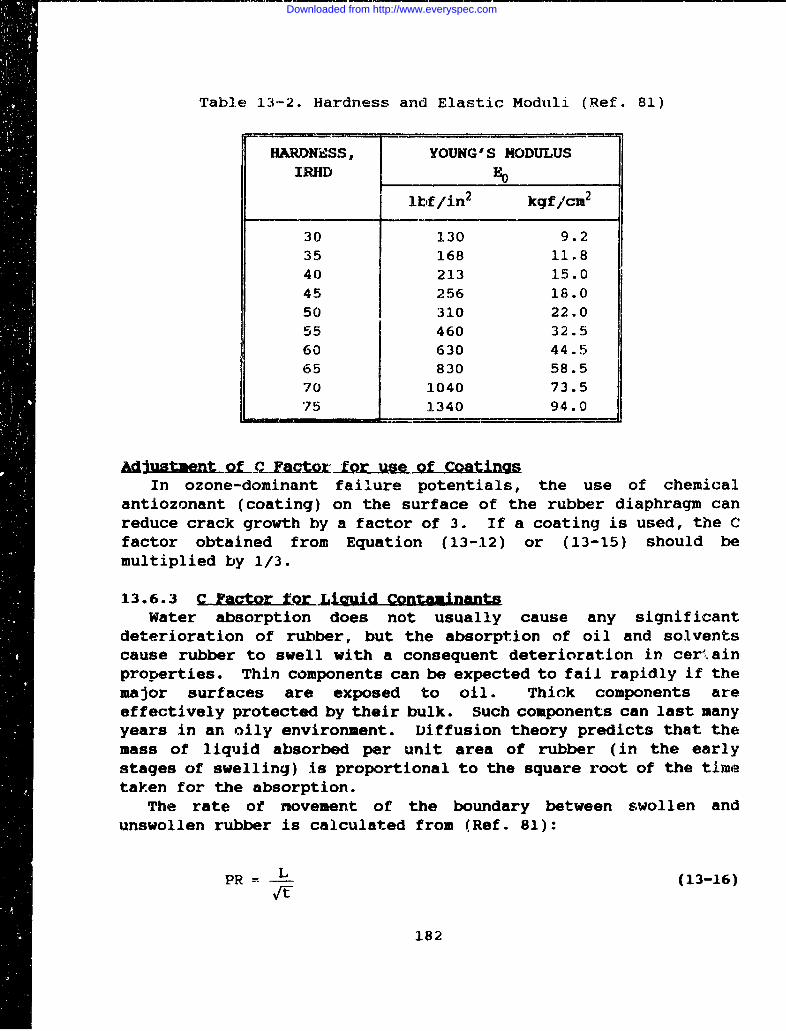
Table 13-2. Hardness and Elastic Moduli (Ref. 81)

HARDNESS, YOUNG'S MODULUSIRHD F- _

lbf/in2 kgf/cm2

30 130 9.235 168 11.840 213 15.045 256 18.050 310 22.055 460 32.560 630 44.565 830 58.570 1040 73.5'75 1340 94.0

A~djustsent of C at••oxugof Coatings

In ozone-dominant failure potentials, the use of chemicalantiozonant (coating) on the surface of the rubber diaphragm canreduce crack growth by a factor of 3. If a coating is used, the Cfactor obtained from Equation (13-12) or (13-15) should bemultiplied by 1/3.

13.6.3 C Factor fQr .Liquid ContaxinantsWater absorption does not usually cause any significant

deterioration of rubber, but the absorption of oil and solventscause rubber to swell with a consequent deterioration in cer",ainproperties. Thin components can be expected to fail rapidly if themajor surfaces are exposed to oil. Thick components areeffectively protected by their bulk. Such components can last manyyears in an oily environment. Diffusion theory predicts that themass of liquid absorbed per unit area of rubber (in the earlystages of swelling) is proportional to the square root of the timetaken for the absorption.

The rate of movement of the boundary between swollen andunswollen rubber is calculated from (Ref. 81):

PR L (13-16)

182


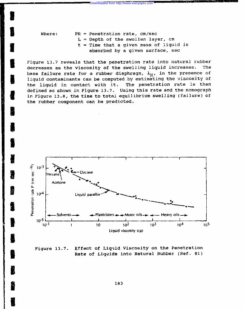
I Where: PR = Penetration rate, cm/secL = Depth of the swollen layer, cmt = Time that a given mass of liquid is

absorbed by a given surface, sec

I Figure 13.7 reveals that the penetration rate into natural rubberdecreases as the viscosity of the swelling liquid increases. Thebase failure rate for a rubber diaphragm, AD1 , in the presence ofliquid contaminants can be computed by estimating the viscosity ofthe liquid in contact with it. The penetration rate is then

I defined as shown in Figure 13.7. Using this rate and the nomographin Figure 13.8, the time to total equilibrium swelling (failure) ofthe rubber component can be predicted.

II

10i-3 Decane *!E

Acetorne *

S104 - Liquid paraffin -- Ir

.,---Solvents-.- .-*-Plasticizers --. *-Motor oils* ... ---- Heavy oils-i.

1(- L -- I-. I ________I

1 1 10 102 103 104 105

Liquid viscosity (cp)IFigure 13.7. Effect of Liquid Viscosity on the Penetration3 Rate of Liquids into Natural Rubber (Ref. 81)

I


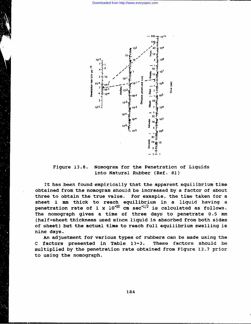
.- 300 .1)10

102 r 30 109

10•1

103- 10 , 3 10

/ I 107

-- • ~2-10 lo 1•1 • _-

I- O4 (r2 10.1 - 1 1067 2, 11 30

;72 110 3 ,

10- -- 1.

10-51 to-2

104

30Sl0-4 10 103

10- '

3-1()-5 102

30

i10 10~3•

Figure 13.8. Nomogram for the Penetration of Liquidsinto Natural Rubber (Ref. 81)

It has been found empirically that the apparent equilibrium timeobtained from the nomogram should be increased by a factor of aboutthree to obtain the true value. For example, the time taken for asheet 1 mm thick to reach equilibrium in a liquid having apenetration rate of I x l0"10 cm sec"1 /2 is calculated as follows.The nomograph gives a time of three days to penetrate 0.5 mm(half-sheet thickness used since liquid is absorbed from both sidesof sheet) but the actual time to reach full equilibrium swelling isnine days.

An adjustment for various types of rubbers can be made using theC factors presented in Table 13-3. These factors should bemultiplied by the penetration rate obtained from Figure 13.7 priorto using the nomograph.

184


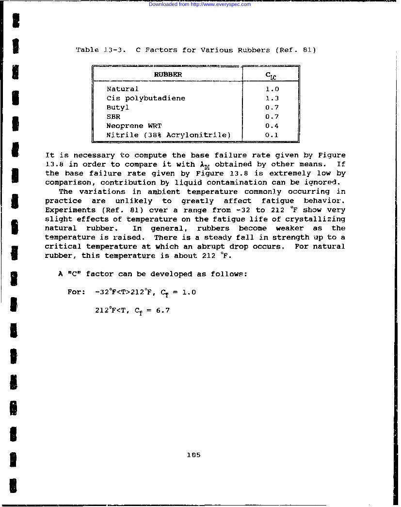
UTable 13-3. C Factors for Various Rubbers (Ref. 8.1.)

RUBBER CLC

Natural 1.0Cis polybutadiene 1.3Butyl 0.7SBR 0.7Neoprene WRT 0.4Nitrile (38% Acrylonitrile) 0.1

It is necessary to compute the base failure rate given by Figure1.3.8 in order to compare it with ADI obtained by other means. IfU the base failure rate given by Figure 13.8 is extremely low bycomparison, contribution by liquid contamination can be ignored.

The variations in ambient temperature commonly occurring inpractice are unlikely to greatly affect fatigue behavior.Experiments (Ref. 81) cver a range from -32 to 212 OF show veryslight effects of temperature on the fatigue life of crystallizingnatural rubber. In general, rubbers become weaker as thetemperature is raised. There is a steady fall in strength up to a

critical temperature at which an abrupt drop occurs. For naturalrubber, this temperature is about 212 OF.

3 A "C" factor can be developed as follows:

For: -32°F<T>212 0 F, CT = 1.0

I 212 0F<T, CT = 6.7

1II

3 185

I



186


I

I ICHAPTER 14

ELECTRIC MOTORSI14.1 INTRODUCTION

Electric motors play a very important part in supplying powerfor all types of domestic and industrial applications. Theirversatility, dependability, and economy of operation cannot beequaled by any other type ou a power unit. It is estimated thatover 90 percent of industrial motive power applications utilizeelectric motors (Ref. 80). Many types are available, thereforemotors are classified in various ways. There are general purpose,special purpose, and definite purpose types of motors. They are

I also classified according to the type of electricity they require;a motor may operate on direct current (DC) or alternating current(AC). If AC, it may be single or polyphase.

This section contains failure rate models that apply to allelectric motors which can be used to support the development ofmechanical equipment and provide a reliability estimate for a new

I design, proposed design modification, or application other thanverified specification parameters. The models are intended tofocus attention on further design analysis which should be

I accomplished to assure the allocated reliability of the motor inits intended operational environment.

I 14.2 CHARACTERISTICS OF ELECTRICAL MOTORS

14.2.1 Ty•sQof._W .otor.DC motors are classified as either series-wound, shunt-wound, or

compound-wound. In the series-wound motor, fie1i( windings whici,are fixed to the stator frame, and the armature windings which areplaced around the rotor, are connected in series so that allcurrent that passes through the field windings also passes throughthe armature windings. In the shunt-wound motor, the armature andfield are both connected across the main power supply (in parallel)so that the armature and field currents are separate. Thecompound-wound motor has both the series and shunt field windings.These may be connected so that the currents are flowing the samedirection in both windings, called "cumulative compounding", or sothat the currents are flowing in opposite directions, called

3 187

I


"differential compounding".

14.2.2 Iypys of Polba se AC MotoraThe most extensively used polyphase motors are the induction

type. The "squirrel cage" induction motor has a wound statorconnected to an external source of AC power and a laminated steelcore rotor with heavy aluminum or copper conductors set into thecore around its periphery while being parallel to its axis. Theseconductors are connected together at each end of the rotor by aheavy ring, providing closed paths for currents induced in therotor to circulate. The rotor windings are not connected to thepower supply.

The wound-rotor type of induction motor has a squirrel cage anda series of coils set into the rotor which are connected throughslip-rings to external variable resistors. By varying theresistance of the wound-rotor circuits, the amount of currentflowing in the circuits, and therefore the speed of the motor, canbe controlled. Induction motors are manufactured with a wide rangeof speed and torque characteristics.

The synchronous motor is the other type of polyphase AC motor.Unlike the induction motor, the rotor of the synchronous motor isconnected to a DC supply which provides a field that rotates instep with the AC field in the stator. The synchronous motoroperates at a constant speed throughout its entire load range,after having been brought up to this synchronous speed. This speedis governed by the frequency of the power supply and the number ofpoles in the rotor.

14.2.3 TyMes of Single-Phase AC MotorsMost of the single-phase AC motors are induction motors

distinguished by different arrangements for starting. Single-phasemotors are used in sizes up to about 7 1/2 horsepower for heavystarting duty chiefly in home and commercial appliances for whichpolyphase power is not available.

The series wound single-phase motor has a rotor winding inseries with the stator winding as in the series-wound DC motor.Since this motor may also be operated on direct-current, it iscalled a "universal motor". The series wound motor has a highstarting torque and is used in vacuum cleaners, sewing machines,and portable tools. In the capacitor- start single-phase rotor, anauxiliary winding in the stator is connected in series with acapacitor and a centrifugal switch. During the starting andaccelerating period the motor operates as a two-phase induction

188


I

SI motor. At about two- thirds full-load speed, the auxiliary circuitis disconnected by the switch and the motor then runs as a singlephase induction motor. In the capacitor-start, capacitor-runI motor, the auxiliary circuit is arranged to provide high effectivecapacity for high starting torque and to remain connected to the3 Iline, but with reduced capacity during the running period. In thesingle-value capacitor or capacitor split-phase motor, a relativelysmall continuously-rated capacitor is permanently connected in oneof the two stator windings and the motor both starts and runs likea two-phase motor.

In the repulsion-start single-phase motor, a drum-wound rotorI circuit is connected to a commutator with a pair of short-circuitedbrushes set so that the magnetic axis of the rotor winding isI inclined to the magnetic axis of the stator winding. The currentflowing in this rotor circuit reacts with the field to produce astarting and accelerating torque. At about two-thirds full loadspeed the brushes are lifted, the commutator is short circuited andI the motor runs as a single-phase squirrel-cage motor. Therepulsion motor employs a repulsion winding on the rotor for bothstarting and running. The repulsion-induction motor has an outerwinding on the rotor acting as a repulsion winding and an innersquirrel cage winding. As the motor comes up to speed, the inducedrotor current partially shifts from the repulsion winding to thesquirrel cage winding and the motor runs partly as an inductionmotor.3 mIn the split-phase motor, an auxiliary winding in the stator isused for starting with either a resistance connected in series withthe auxiliary winding (resistance-start) or a reactor in serieswith the main winding (reactor-start). The split-phase motor isused in refrigerators, air conditioners, freezers, and other5 compressors involving high starting load.

1.4.3 FAILURE MODESFailure rate models included in this section are based upon

identified failure modes of the individual parts. Typical failuremodes and their failure causes and effects are listed in Table 14-£ 1. Failure rate models or estimates for the following componentparts are discussed or referenced in this section:

I. Bearings2. Windings3. Brushes4. Armature (shaft)5. Stator Housing (casing)

3 189

I


Table 1i4-1. Electric Motor Failure Modes

ELECTRIC MOTOR FAILURE MODES

COMPONENT FAILURE MODE FAILURE CAUSE FAILURE EFFECT

BALL OR ROLLER WORN OUT POOR NOISY; HEATBEARING a) SPALLING LUBRICATION; BUILD-UP;

b) CREEPING OR CONTAMINATION; ARMATURESPIN OVERLOADING; RUBBING

OR HIGH STATOR;TEMPERATURE SEIZED

ELECTRICAL a) OPEN EXCESSIVE HIGH MOTOR WON'TWINDINGS b) SHORT TEMPERATURE RUN(ROTOR ORSTATOR) SPARKING AT

BRUSHES

HOUSING a) CRACKED FATIGUE; LEAKAGE OREXTERNAL DUST INTOSHOCK; MOTOR; SHORTEDVIBRATION OR SEIZED

ARMATURE a) SHEARED FATIGUE; SEIZED;SHAFT MISALIGNMENT; ARMATURE

b) CRACKED OR BEARING RUBBING STATORROTOR FAILURELAMINATIONS

BRUSHES WORN OUT IMPROPER EXCESSIVEMAINTENANCE; SPARKING;CONTAMINATION; CHATTER ORHITH HISSING NOISE;TEMPERATURE; MOTOR RUNS TnOLOW FAST OR TOOATMOSPHERIC SLOW UNDERHUMIDITY; LOADIMPROPERCONTACTPRESSURE

SLEEVE BEARING WORN OUT EXCESSIVE LOAD SEIZED; NOISY;(BELT HEAT BUILD-UP;TENSION); TOO ARMATUREFREQUENT RUBBING STATORSTAR13 AkNDSTOPS UNDERHEAVY LOADS;POORLUBRICATION

190


I

A I The models developed in this chapter will be based on an ACfractional horsepower (FHP) type motor, although it will fe generalenough to be applied to most motors. Therefore, a specifi(. motorbeing analyzed may not need to include all' the failure vates due I.-,its lack of certain parts (e.g., brushes).

14.4 MODEL DEVELOPMENTThe model developed is based on a fractional or integral3 horsepower AC type motor, although it will be qeneral enough to be

applied to most motors.The reliability of an electric motor is dependent upon the

- reliability of its parts, which may include: bearings, electricalwindings, armature/shaft, housing, and brushes. Failure mechanismsresulting in part degradation and failure rate distribution (as aI function of time) are considered to be independent in each failurerate model. The total motor system failure rate is the sum of the5 failure rates of each of the parts in the system:

Ax = IBE + IWI + BS + A + AST + IGE (14-1)

I Where: N= Total failure rate for the motor system,failures/million hours

IBE = Total failure rate for bearings,failures/million hours

AW1 Total failure rate for electric motorI windings, failures/million hoursXBS = Total failure rate for brushes,

failures/million hoursIA = Total failure for the armatur'e shaft,failures/million hours

IST = Total failure for the stator housing,'I failures/million hoursAGE = Total failure for gears, failures/million

3 hours

The failure rates for all the parts in the motor system must besummed before the system failure rate can be found. Failure ratemodels for shafts, housing (casings), gears, and bearings can befound in Chapters 10, 8, and 7, respectively. A failure rate model3 for brushes is under development.

13 191

I


14.5 FAILURE RATE MODELS FOR MOTOR WINDINGSThe electric motor windings failure rate, AIW, is derived by

Equation (14-2):

SAWl = WI,B CT * Cv • Cf • Calt (14-2)

Where:XWI,B = Base failure rate of the electric motor

windings, failures/million hoursCT = Multiplying factor which considers the

effects of ambient temperature on the basefailure rate

Cv= Multiplying factor which considers theeffects of electrical source voltagevariations

Cf= Multiplying factor which considers theeffects of electrical source frequencyvariations

Calt = Multiplying factor which considers theeffects of operation at extreme elevationss

kWI,B is the base failure rate of the specific motor as suppliedby the motor manufacturer. For fractional horsepower motors, itcan be estimated from Equation (14-9). The C factors are describedin the following paragraphs.

14.5.1 TemperatureHeat is the primary limiting factor of motor windings. Heat

causes the windings to age and deteriorate, so after time theybreak down and lose their insulation quality. When this happensthe related electrical components "short" and the motor burns outor blows a fuse.

Under normal operating conditions, the insulation material usedin the windings of electric motors is generally reliable, therebymaking the windings themselves a reliable component.

The life of any given insulation material depends on the degreeof heat to which it is exposed. Equations (14-3) through (14-6)reflect the temperature C factors for four insulation classes, itshould be noted that the insulation life increases beyon! normallife expectancy as temperature is dropped below the ratedtemperature. Also, these factors were developed from NEMA standardsfor drip-proof and totally enclosed fan-cooled, integral horsepowermotors with 1.0 Service Factor.

192


-I Cla,:in A normlizecd at 1.05 0C

SI • (5 2 X "o.5) e°0 3('r*6s) (14-3)

S• .a B Insulation, normalized at 130 "C

CT = (1.4 X ;0-5) eo'°A6(T÷9•) (14-4)

SClass F Insulation, normalized at 155 OC

--I CT= (1.5 X I0-1 eo°'s 9 (tS) (14-5)

3I , Class 11 Insulation, normalized at 180 "C

CT = (9.8 X IC"-5) e °1.01(T-1 4 0) (14-6)

Where: T = Ambient temperature during full loadoperation, OC

rhe winding temperature is determined by measuring both theambient and the hot temperature resistances of the windings. Theresistance measurement gives an average temperature which is morerepresentative than spot measurements with a thermometer. Thismethod has become standard because of the dimensional restrictionsof so many motor designs, which prevent the use of thermometers.5 Since variation in ambient temperatures during operation is mo-econvenient to estimate, Equations (14-3) through (14-6) above havebeen adjusted for the maximun allowable temperature rise byresistance and windinas "hot spot" temperature for each insulationclass. The equations emphasize tho importance of avoiding motoroverloads in order to maximize insulation life. However, shortpeak IGads involvs such & short time that their effect oniinsulation life is iegligible.

The correction factor for the wirnings of a fract. onalhcr~e.ower motor for virying ambient temperatures is given by:

3 193

-I


S= 10O•' - (14-7)CT 101F7To + 1273 -T ÷2731 147

Where: T = Ambient temperature during operation, °CTo = Ambient temperature rating of windings, OC

14.5.2 Temperature Cyclin*In many instances, a motor is not run in a steady state

temperature environment. Many MIL-STD testing pi.ocedures specifycyclic ambient temperature profiles (i.e., MIL-STD-810D). One suchexample of an elevated ambient cyclic temperature profile is shownin Figure 14.1. A "C" factor for the windings of a fractionalhorsepower motor, given a temperature profile, can be developed bycomputing an "equivalent" winding characteristic life, then"comparing this value to the value normalized at the windings ratedtemperature.

1T T.-273 l l L L--' L3 L..

CT =t + ...+ t+ (14-8)

Where: To = Ambient temperature rating of windings, °Ctj = Time at each temperature interval, i,

representing the number of intervals, hours(See Figure 14-1 for example)

Li = Characteristic winding life at eachtemperature interval, as represented byEquation 14-9 (i representing the number ofintervals), hours

The winding Weibull Characteristic Life for cyclictemperatures can be computed from:

__3 57 1

1 = O Tjt273 (4--9)

Where: Ti - Temperature at each cyclic interval, i,representing the number of intervals, °C(See Figure 14.1 for example)

194


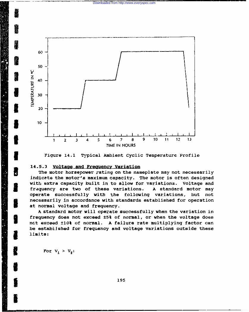
50 -

YuZL 40-

S30"

* 20

.110'. I ii I I • , i , I i.I , .- 1..- -

1 2 3 4 5 6 7 8 9 10 11 12 13

TIME IN HOURS

Figure 14.1 Trpical Ambient Cyclic Temperature Profile

14.5.3 yQ .jg • Frequency VariationThe motor horsepower rating on the nameplate may not necessarily

indiceate the motor's maximum capacity. The motor is often designedI with extra capacity built in to allow for variations. Voltage and

fraquency are two of these variations. A standard motor mayoperate successfully with the following variations, but not

I necessarily in accordance with standards established for operationat normal voltage and frequency.

A standard motor will operate successfully when the variation inU Q frequency does not exceed ±5% of normal, or when the voltage doesnct exceed ±10% of normal. A failure rate multiplying factor canbe established for frequency and voltage variations outside theseI i limits:

For V, >

£ 195

I|


V A __ oio x 100Cv = 0. 01 100 - VR 21-0

Where: VR = Rated VoltageVA = Actual Voltage

For VA < VR:

VR VA 10Cv = 0.01 00 + R (14-11)

For FA > FR:

Cv = 0.01 100 - FR _ (14-12)

Where: FR = Rated FrequencyFA = Actual Frequency

For FA < FR:

FR -F 0Cv = 0.01 (00 + ) (14-13)

14.5.4 AJtiM1fThe influence of altitude on the life of a fan-cooled motor may

be tabulated based on a 50% reduction in life for every 100Cincrease in temperature. Table 14.-2 is a tabulation of failurerate multipliers for altitude/temperature conditions applicable tofan-cooled motors which are not enclosed. For totally encloseamotors, altitudes to 60,000 feet will not influence life as

196


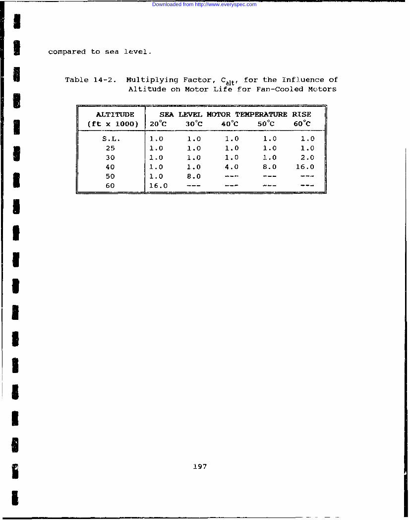
I compared to sea level.

I Table 14-2. Multiplying Factor, Cal, for the Influence ofAltitude on Motor Life for Fan-Cooled Motors

ALTITUDE SEA LEVEL MOTOR TFE4PERATURE RISE3 (ft x 1000) 20-C 30 0C 40 0C 50 0C 60'C

S.L. 1.0 1.0 1.0 1.0 1.025 1.0 1.0 1.0 1.0 1.030 1.0 1.0 1.0 1.0 2.040 1.0 1.0 4.0 8.0 16.050 1.0 8.0 ---.. ..

60 16.0 ---

1I

IUIIIII

5 197

I


THSPU NETONLYLF LN

IIIIiI

19I


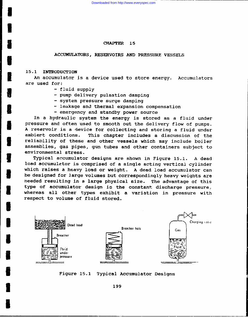
I

ACCUMULATORS, RESERVOIRS AND PRESSURE VESSELS

15.1 INTRODUCTIONAn accumulator is a device used to store energy. Accumulators

are used for:- fluid supply- pump delivery pulsation damping- system pressure surge damping- leakage and thermal expansion compensation- emergency and standby power source

In a hydraulic system the energy is stored as a fluid underpressure and often used to smooth out the delivery flow of pumps.A reservoir is a device for collecting and storing a fluid underambiert conditions. This chapter includes a discussion of theI reliability of these and other vessels which may include boilerassemblies, gas pipes, gun tubes and other containers subject toenvironmental stress.

Typical accumulator designs are shown in Figure 15.1. A deadload accumulator is comprised of a single acting vertical cylinderI which raises a heavy load or weight. A dead load accumulator canbe designed for large volumes but correspondingly heavy weights areneeded resulting in a large physical size. The advantage of thistype of accumulator design is the constant discharge pressure.whereas all other types exhibit a variation in pressure withrespect to volume of fluid stored.I

Charr~ing 'alhDead load B

BrcaBhar ho le

Is

Fluid"--

I Figure 15.1 Typical Accumulator Designs

3 199

I


A spring loaded accumulator contains a spring whi.ch moves withina cylinder. As the volume of fluid in the accumulator isincreased, the spring is compressed and the spring force isincreased. The minimum pressure in the accumulator depends on thedesigned spring preload. The advantage of this design is itssimplicity. The piston stroke and, therefore, the volume of fluidwhich can be stored is limited by the physical characteristics ofthe spring.

A gas loaded accumulator is designed to utilize a compressed gassuch as nitrogen or air to pressurize the stored fluid. A pistonor bag is tised to separate the fluid and gas. Gas loadedaccumulators can be very large. As discussed in the next section,accumulators are usually designed to be operated in the verticalposition. The fluid pressure as a function of fluid volume in agas loaded accumulator depends upon many factors such as the gasbeing used, the temperature of the gas and its pressure - volumecharacteristics.

15.2 FAILURE MODESIn any type of accumulator utilizing a piston the cylinder bore

has to be machined, and wear will occur between the piston andcylinder body. Seals are built into the piston and these aresubject to wear and leakage. Depending on the accumulatorapplication, response time may be a factor. The response of thedead load accumulator will be somewhat slow due to the high inertiaof the load and piston. The response of spring loaded accumulatorswill depend on the age of the spring and its modulus of rigidity.A response of a piston type accumulator will be adversely affectedby the inertia of the piston and the effect of seal stiction.

Although a piston type accumulator can be used inclined to thevertical, the rate of wear will be increased due to the additionalside load. Failure of a piston type accumulator tends to begradual caused by deterioration of piston seals and wear in thecylinder bore. Failure of a bag type gas loaded accumulator willbe more sudden caused by the rupturing of the bag or diaphragm.The failure rate of a bag type accumulator may also depend on itsphysical characteristics, a tall narrow unit subject to suddendischarge could cause the poppet valve to lock closed a partiallydischarged unit.

A spring loaded accumulator must be evaluated closely forreliability to verify compatibility between the spring material andthe surrounding medium. Any leakage past the seal could have adeteriorating effect on the spring material and its compression

200


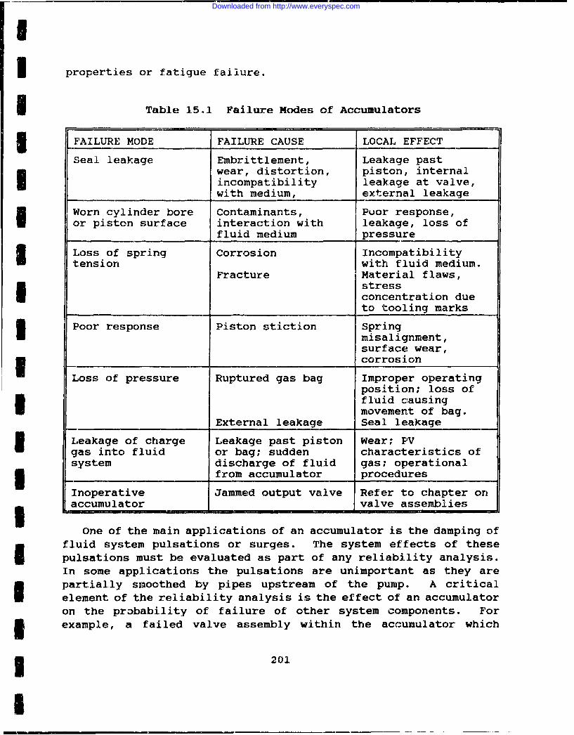
I

3 properties or fatigue failure.

SI Table 15.1 Failure modes of Accumulators

3 FAILURE MODE FAILURE CAUSE LOCAL EFFECT

Seal leakage Embrittlement, Leakage pastwear, distortion, piston, internalincompatibility leakage at valve,with medium, external leakage

Worn cylinder bore Contaminants, Puor response,or piston surface interaction with leakage, loss of

fluid medium pressure

Loss of spring Corrosion Incompatibilitytension with fluid medium.

Fracture Material flaws,stressconcentration dueto tooling marks

Poor response Piston stiction Springmisalignment,surface wear,corrosion

Loss of pressure Ruptured gas bag Improper operatingposition; loss offluid causingmovement of bag.

External leakage Seal leakage

S Leakage of charge Leakage past piston Wear; PV

gas into fluid or bag; sudden characteristics ofsystem discharge of fluid gas; operational3 from accumulator procedures

Inoperative Jammed output valve Refer to chapter onaccumulator valve assemblies

One of the main applications of an accumulator is the damping offluid system pulsations or surges. The system effects of thesepulsations must be evaluated as part of any reliability analysis.In some applications the pulsations are unimportant as they are

I partially smoothed by pipes upstream of the pump. A criticalelement of the reliability analysis is the effect of an accumulatoron the probability of failure of other system components. For3 example, a failed valve assembly within the accumulator which

3 201

I


prevents fluid discharge may not be immediately detected and damageto other components may occur due to pressure transients. Shockwaves produced as a result of the sudden closing of a downstreamvalve, for example, travels through the system fluid to the far endUof the system and a decompression wave is formed which travels backto the valve. These waves travel back and forth until the energyis expended. The more rapid the valve closure, the more severe thepressure transient generated. Without detection of an accumulatorfailure, severe degradation and damage to system components couldbe occurring without operator or maintainer knowledge.

15.3 FAILURE RATE CONSIDERATIONS

15.3.1 9elSpecific failure modes of seals and procedures to determine

their failure rates under different operating environments arediscussed in Chapter 3. Of particular interest in the designevaluation of accumulators and other pressure vessels is the Icompatibility of the fluid medium and the seal material. Theposition of the accumulator in the fluid system must also be knownto determine the side load on the piston and corresponding stresson the seal.

15.3.2 S• ig

Specific failure modes of springs and procedures to determinetheir failure rates under different operating environments are 5discussed in Chapter 3. For most accumulators the failure rateequations for static springs can be assumed. The reliability of aspring is very sensitive to corrosion and the compatibility of the 3fluid and spring material must be considered.

15.3.3 FistQnDCylinder iThe wear rate of the piston surface and cylinder bore will be

sensitive to the position of the accumulator in its operatingenvironment. Tilting of the accumulator from its vertical position Iwill alter the side load of the piston. This parameter and otherseffecting the reliability of the piston/cylinder are included inthe reliability equations contained in Chapter 9.

15.3.4 yals 3The reliability of valve assumblies which may be contained

within the accumulator is determined using the equations containedin Chapter 6. One particular failure mode to be considered in the m

202 3

I


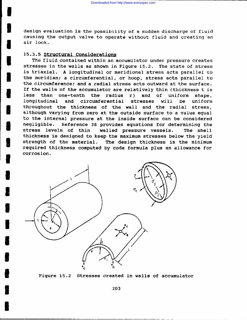
I

SI design evaluation is the possibility of a sudden discharge of fluidcausing the output valve to operate without fluid and creating an

I air lock.

15.3.5 StutrlCnieain3 The fluid contained within an accumulator under pressure createsstresses in the walls as shown in Figure 15.2. The state of stressis triaxial. A longitudinal or meridional stress acts parallel tothe meridian; a circumferential, or hoop, stress acts parallel tothe circumference; and a radial stress acts outward at the surface.E If the walls of the accumulator are relatively thin (thickness t isless than one-tenth the radius r) and of uniform shape,longitudinal and circumferential stresses will be uniformI throughout the thickness of the wall and the radial stress,although varying from zero at the outside surface to a value equalto the internal pressure at the inside surface can be consideredI negligible. Reference 38 provides equations for determining thestress levels of thin walled pressure vessels. The shellthickness is designed to keep the maximum stresses below the yieldU strength of the material. The design thickness is the minimumrequired thickness computed by code formula plus an allowance forI corrosion.I

, L

* CT

SFigure 15.2 Stresses created in walls of accumulator

3 :203

l


The bursting effect of internal fluid pressure creates acircumferential pressure in the wall of the accumulator. Totalforce acting on a half cylinder as shown in Figure 1.5.1 is:

FC = 2PriL (15..-i)

Where: P = Internal pressureri = Internal radius

L = Cylinder length

The resistive force due to ciroumferential stress, ac acting onthe cylinder wall to achieve equilibrium must equal force F.

Fc = 2atL.

Substituting Fc in equation 15-1 for equation 15-2 provides thefollowing relation:

cc = Pri/t (15-3)

This equation provides the maximum circumferential stress in thevessel wall on the assumption that end closures provide no support,such as is the case for long cylinders or tubes. The equilibriumof forces in the longitudinal direction gives:

F1 = wPr 2 (15-4)

and the corresponding longitudinal stress is:

al = Pr 1 /2t (15-5)

The effects of end plates and joints on the accumulator is areduction in strength of the accumulator due to riveted joints,welding and other fabrication techniques. This reduction isaccounted for by including a joint efficiency parameter, n, in thecircumferential stress equation and qC in the equation forlongitudinal stress.

minimum strength of jointstrength of solid material

This addition provides the following equations:

204


I

ac = Pri/til, (15-6)

U and:aI - Pri/2tqc (15-7)

U The relative strength (efficiency) of a joint depends upon itsdesign and type of joint. Table 15-2 provides efficiencies that

* may be expected in the various types of joints if they are welldesigned.

I TABLE 1M-2 APPROXIMATE EFFICIENCIES OF JOINTS(References 57 and 58)

TYPE OF JOIWT DESIGN INSPECTION EFrICIENCy

Single Sample-Full 50 - 60%Riveted Lap Joint Double 60 - 70%

Triple 70 - 80%

Riveted Butt Joint Single Sample-Full 6' - 70%Double 75 - 83%Triple 80 - 89%3 Quadruple 85 - 94%

Welded Butt Joint Single Not radio- 65 - 90%graphed to

Double Fully 70 - 100%I radiographedI

I The actual value for the efficiency parameter from Table 15-2 willdepend on the confidence level in manufacturing techniques andquality control.

The ends of the accumulator are often hemispheres. The internalpressure in a thin spherical shell will create two mutuallyperpendicular circumferential stresses of equal magnitude and aradial stress. Again a thickness/radius ratio of less than 1/10provides a minimal value of radial stress. The force on thehemisphere due to internal pressure P is:

Fc- wrP2 (15-8)

I and the resistive force due to circumferential stress is:

Fc W 2wrtac (15-9)

3 205

I


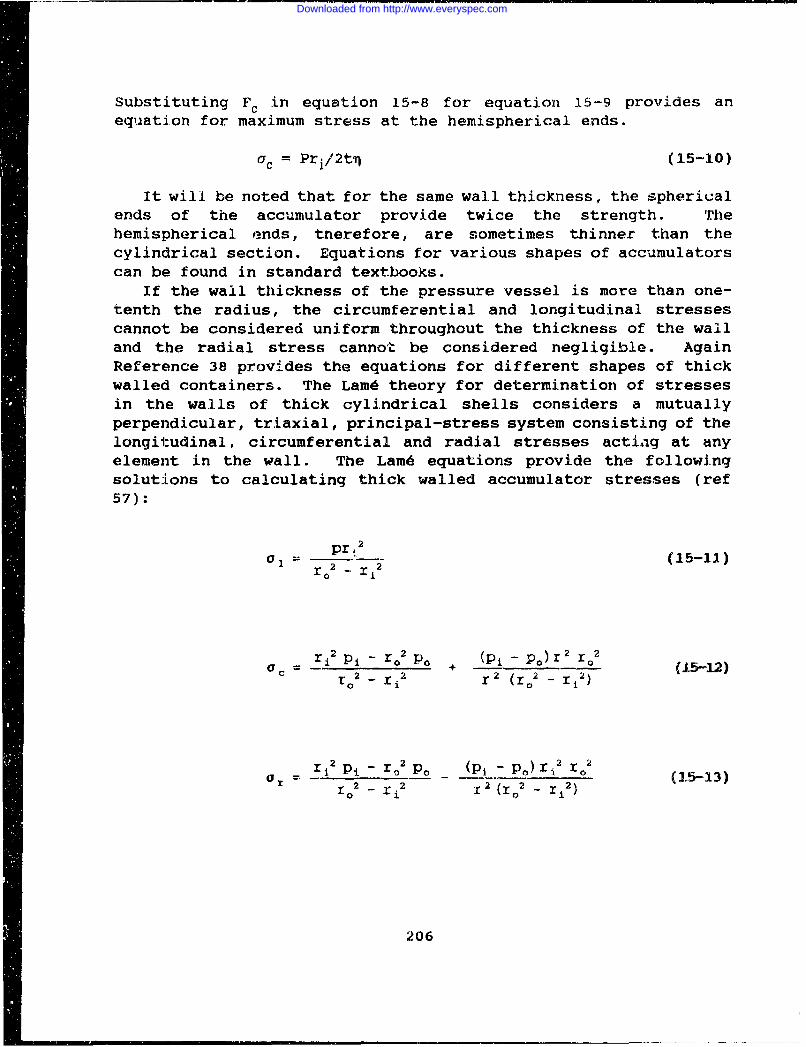
Substituting Fc in equation 15-8 for equation 15-9 provides anequation for maximum stress at the hemispherical ends.

cc = Pri/2tq (15-10)

It will be noted that for the same wall thickness, the sphericalends of the accumulator provide twice the strength. Thehemispherical ends, tnerefore, are sometimes thinner than thecylindrical section. Equations for various shapes of accumulatorscan be found in standard textbooks.

If the wall thickness of the pressure vessel is more than one-tenth the radius, the circumferential and longitudinal stressescannot be considered uniform throughout the thickness of the walland the radial stress cannot be considered negligible. AgainReference 38 provides the equations for different shapes of thickwalled containers. The Lam6 theory for determination of stressesin the walls of thick cylindrical shells considers a mutuallyperpendicular, triaxial, principal-stress system consisting of thelongitudinal, circumferential and radial stresses acting at anyelement in the wall. The Lam6 equations provide the followingsolutions to calculating thick walled accumulator stresses (ref57):

m 2pr1- (15-1i1)

0 2 __- r 2

= r1 2 Pi 1 r 2 PO (p - p) r 2 (15-12)ro 2

-ri o2r 0

2 - I2)

or = -2 o22O• p= - -P Pj P r 2 r (15-13)1o 2 - I2 2 (io2 - 112)

206


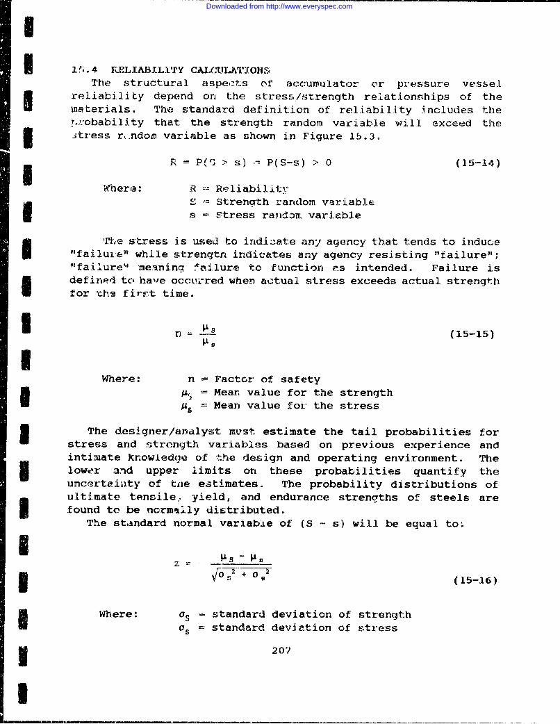
I

I 1 5.4 ]RELIABILITY CAL(ChIA' rONSThe structural aspects of accumulator or pressure vessel

reliability depend on the stress/strength relationships of thematerials. The standard definitoion of reliability fincludes ther,,2.obability that the strength random variable will exceed theAtress r,..ndom variable as shown in Figure 15.3.

R = P(13 > s) - P(S-S) 0 (15-14)

Where: R ReliabilitvS Strencgth random variables Stress randon. variable

The stress is used to indizate any agency that tends to induce"failuile"11 while strength indicates any agency resisting "failure";"failure' meaning failure to function as intended. Failure isdefined to havre occurred when actual stress exceeds actual strengthfor tJhe firrt time.

n IS (15-15)

Where: n = Factor of safety• = Mean value for the strengthAS = Mean value for the stress

The designer/analyst must estimate the tail probabilities forstress and strength variables based on previous experience andintimate knowledge of the design and operating environment. The

S lower and upper limits on these probabilities quantify theuncertainty of tne estimates. The probability distributions ofultimate tensile, yield, and endurance strengths of steels arefound to be ncrmaily distributed.

The standard normal variabie of (S - s) will be equal to,

VS +Go(15-16)

Where: aS standard deviation of strengthas= standard deviation of stress

I207


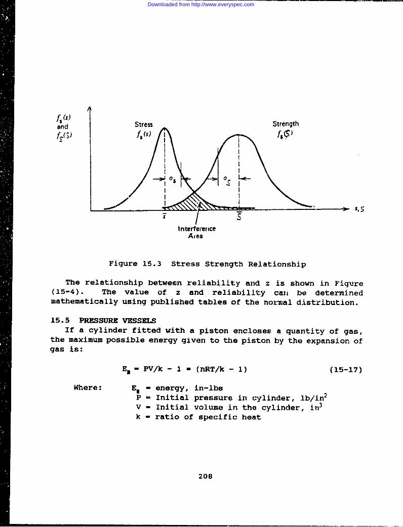
fs (S)and Stress Strength

f) f(s) I

~- 311 as as-< II

InterferenceArea

Figure 15.3 Stress Strength Relationship

The relationship between reliability and z is shown in Figure(15-4). The value of z and reliability can be determinedmathematically using published tables of the normal distribution.

15.5 PRESSURE VESSELSIf a cylinder fitted with a piston encloses a quantity of gas,

the maximum possible energy given to the piston by the expansion ofgas is:

El - PV/k - 1 - (nRT/k - 1) (15-17)

Where: E - energy, in-lbsP Initial pressure in cylinder, lb/in2V - Initial volume in the cylinder, in 3

k = ratio of specific heat

208


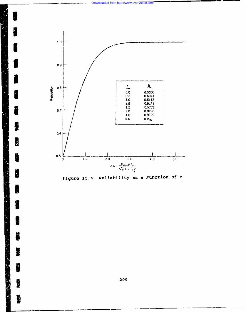
II ~~ ~ ~~1.0 ________

I 0.9

0.0 0.5000U.5 0.6914.r .0 0.8413

1.5 0.9W3 12., 0. 772

0.7 30 0,99864.0 0,99999--- 5.0 0.9161

0.5

0 ,.' 2.0 3.0 4.0 5.0

Figure 15.4 Reliability as a Function of z

UJI'

I

IU

5 209


II

!I

THISPAG INTNTINALY LET. LAN

21I

Im


II

CHAPrER 16

THREADED FASTENERS

1.6.1 INTRODUCTIONMethods of fastening or joining components include threaded

fasteners, welding, brazing, soldering, and various adhesivebonding systems. One advantage of threaded fasteners is that theypermit disassembly of the equipment for maintenance and repair.Threaded fasteners also allow the use of automated as well asstandard manual tools for assembly and installation procedures evenunder restricted conditions. And significantly, the multitude ofavailable sizes, materials, finishes, and strength levels ofmechanical fasteners provides a strong design support system foroptimum structural compatibility, even under wide environmentalextremes. The reliability of threaded fasteners in a givenoperating environment depends on the strength of materials, methodsof fabrication and assembly, and the stress levels created byfatigue loads and environmental conditions. This chapter considersE the reliability performance of externally and internally threadedfasteners.

I 16.1.1 Externally MThread% FatenersBolts and screws are fasteners with a formed head on one end and

an external thread on the other end. Studs are fasteners thatincorporate external threads at each end. Structural bolts andscrews are installed through prepared holes in the material, to bejoined. Various lengths of bolts and screws are produced toaccommodate the thickness of the material to be fastened and theadditional length of thread needed for proper engagement with thenut or with the internal tapped thread. These fasteners aresubjected to tensile, shear, bending, and fatigue loads sensed bythe joint. They also respond to the environment imposed on thejoint, which may include temperature extremes or exposure tovarious corrosive conditions.

Studs represent a special class of externally threadedfasteners, and a number of configurations have found wide use indesign. Double-end studs are threaded at both ends; they can bemated with two nuts, or one end of the stud can be installed in atapped hole and a nut employed on the other end to tighten or

3 211

I


secure the joint. Another configuration is the continuous-threadedstud, which has been utilized both in general-purpose joining andin special classes for high-temperature and/or high-pressurebolting.

16.1.2 Intn•h•f b atd _ erdiSpecific fastening devices which incorporate internal (female)

threads include nuts and inserts. They are intended to engage withthe external threads of bolts, screws, and studs, and should becompatible to develop the full rated strength of the externalthread.

One aspect of threaded fastener performance that is of concernis the fastener's susceptibility to loosening as a result of severevibration or dynamic loadings acting on the joint. Since vibratorystresses cannot be totally eliminated, several methods have beendeveloped which have proven effective in maintaining fastenerintegrity.

Self-locking nuts are integral fasteners which incorporatein the nut element a controlled high-torque feature which isdesigned to prevent rotation off the external threads, even if theinitial tightening torque is completely relaxed. The sameprinciple of an inherent self-locking feature is often extended toscrews used in tapped holes.

. Chemical thread-locking systems include anaerobic and epoxyadhesives which are applied to the fastener threads beforeinstallation, and which cure and effect a permanent bond afterassembly.

Cotter pins are a supplemental locking device used with aslotted or castellated nut. They are installed through a drilledhole in the bolt threads to prevent rotation or movement of the nutafter installation.

Safety lock wiring is also a supplemental locking system.Usually two or more fasteners in series must be wired to preventrotation in the "off" direction. The nut end can be wired usingslotted or castellated nuts and bolts with drilled holes. However,the predominant use of safety wiring is to secure screw heads whichhave been drilled to accommodate the wire where the screws havebeen installed in tapped or blind holes.

Lockwashers are used to resist the loosening effects ofvibration, and come in a wide variety of designs tor variousapplications. Conical spring washers are typically made ofhardened and tempered steel that is slightly concaved. Thesewashers deform when the bolt is tightened, acting as a spring that

212


I

I compensates for small losses in bolt tension due to thermalexpansion or compression set of the gaskets. Helical springwashers employ a single-coil helical spring that flattens under

I load. The spring action assists in maintaining the bolt load,while the split edges provide a locking action by biting into thebearing surfaces. Toothed lockwashers provide a gripping actionresulting from the teeth biting into the material of the bolt heador nut, and being deformed axially, with the application of tension

I from bolt torquing.All locking systems should be compatible, For example, using an

elastic stop nut (a nut with a deformable plastic insert) on a malethread drilled for use with a cotter pin, may destroy the holdingcapability of the nut because of damage to the insert.

I 16.1.3 Thre.dfInch-series thread forms were developed and used by countries

employing the English system of measurement. In the United States,standards have been predicated on a 600 screw thread angle,originally standardized as the American National thread. Since1948, the accepted standard has been the Unified thread form, whichalso specifies a 600 angle.

The relationship between nominal diameter and the number of3 threads par inch is referred to as the "diameter-pitchcombination." There are several prominent thread forms which coverthe majority of standards intended for general engineering use.

Coarse-thread series. This is perhaps the most widely usedseries of commercial and industrial fasteners. The thread fonm isparticularly advantageous for applications requiring rapid assemblyor disassembly, or for threading into lower-strength materials,such as castings, soft metals, and plastics.

0 Fine-thread series. For the same nominal diameter, thisseries incorporates more threads per inch. The result is a largertensile stress area than that of the same size coarse thread,

I contributing to the greater strength capability of fine-threadfasteners. These fasteners are normally used where the ler~gth ofthread engagement is short, or where a snaller lead angle isdesired. Fine-thread-series fasteners are used extensively inaerospace and in applications where coarse threads would not besuitable.

*Other series include the extra-fine-thread, 8-thread, 12-thread, and 16-thread series.

In addition to establishing diameter-pitch combinations, theUnified screw-thread system also defines the distinct profile and

213

I


identification requirements for several screw-thread forms. Thebasic thread for the bulk of commercial and industrial fasteners isthe Unified form, identified as "UNC" for the coarse-thread seriesand "UNF' for the fine-thread series.

16.2 FAILURE NODES

16.*2.1 J~~rýnJb~J e~nThe phenomenon of hydrogen embrittlement in threaded fasteners

has been mostly associated with high-strength (over 160 ksi) steelparts which have been furnished with either zinc or cadmiumelectroplating. During the plating process, atomic hydrogen can betrapped in or under the plating. Other sources of hydrogen can betraced to material pickling or alkaline or acid cleaning. Unlessthe free hydrogen is removed, when the fastener is used andstressed, as in a structural application, the hydrogen can attackthe grain boundaries. The result is rapid crack propagation andoften catastrophic failure of the steel fastener.

Two major ways to avoid the problems of hydrogen embrittlementare to (1) bake the fasteners in a subsequent operation afterplating to remove the excess hydrogen and (2) use mechanicalplating processes in lieu of electroplating. Mechanical plating isthe process of using glass beads to cold-weld a ductile metal(e.g., cadmium, zinc, etc.) onto a metal substrate by mechanicalenergy. Coating thicknesses are more uniform than when the 'hotdip' process iE used. However, hot-dip fasteners have morecorrosion protection built-in, due to the greater coatingthickness. Usually, it is necessary 'to chase the hot--dip coatedthreads with a die, since the coating is not uniform.

16.,2.2 fLguM

The importance of fatigue strength properties is associated withthe fact that when failure is encountered, it is invariablycatastrophic in nature, arid often occurs without warning. Researchhas established that rolled threads exhibit higher fatigue lifethan machined or ground threads. Further, threads rolled afterheat treatment show better fatigue performance than comparablethreads rolled before heat treatment. In addition, factors such asproper b3olt head design, cold work of the head-to-shank fillet,quality control of the basic material used, and minimization ofpossible metallurgical defects all contribute significantly toimproved fatigue life.

With respect to fatigue performance, it has been observed that

214


I

I failures normally develop at stress levels well below the staticstrength of the fastener. The two main types of joint fatigueloading are shear fatigue and tension fatigue. For shear-loadedjoints, fatigue failure normally occurs in the plate or sheetmaterial. The applied fatigue or dynamic stresses, holepreparation, hole clearance, amount of induced bending, andfastener preload are some of the factors which influence shear

I joint fatigue life.

16.2.3 Tggp~eratizeBoth high-temperature and low-temperature (cryogenic) service

exposures are experienced in practice in nuclear systems,aerospace, electronics, transportation, energy systems,construction, and similar applications.

Characteristically, materials used at cryogenic temperatureswill show an increase in tensile strength, but may sacrificeductility. Conversely, at elevated temperatures, tensile strengthproperties are usually reduced, and above critical servicetemperature limits they may drop off dramatically.

I 16.2.4 Lgad and TorqueFor every fastener system, there is an optimum torque range to

develop the design clamp load. This is normally referred to as t~ie"torque-tension relationship". Over torquing can result inexcessive bolt yielding and possible subsequent relaxation, or eventhread stripping and failure on installation. Too low an initialtorque can contribute to potential fatigue and/or joint looseningwith extended service life.

There are a number of factors which affect and influence thenominal torque-tension relationship, including condition of thethreads, condition and squareness of the joint, method andequipment for torquing, installation from the nut or bolt head end,and lubrication. Possibly the most influential factor is the

I lubrication (plating and/or supplemental lubricant) on the fastenersystem, since the effective coefficient of friction can alter theinstallation torque requirements by as much as 50 to 100 percent.

I 16.2.5 Bolt and Nut CogDatibilityParticularly where high-strength bolts are used, critical

attention must be given to specifying the correct mating nut.Inadvertent specification of a lower-strength (grade) nut invitesthe possibility of nut thread stripping under high tensile loading.But more significantly, a weaker nut will not adequately develop

3 215

I


the full clamp load capability of a high-strength bolt whensubjected to the necessary installation torque.

As a rule of thumb, the thickness (height) of a nut shouldapproximate the diameter of the equivalent mating bolt to developthe full tensile strength properties of the bolt, f the bolt andnut materials have the same strength.

16.2.6 YibrAtinWhereas fatigue loading is presumed to be relatively high with

respect to the strength of the threaded fastener or the joint,vibration loads are relatively low, but may be associated withvarious ranges of cyclic frequencies. Critical combinations offrequency, loading, and amplitude can force a structure intoresonance, often with catastrophic results. While the overwhelmingmajority of operating structures are not subjected to conditions ofresonance, the vibration forces present (including random andsteady-state vibration, shock, and impact) are sometimes seriousenough to drastically affect the threaded fastener system.

Under repeated or extensive vibration, there is a tendency forthe nut to rotate or loosen of f the bolt threads. Continuedvibration can actually result in the nut completely disengagingfrom the bolt, with subsequent loss of the bolt from the joint.Not as severe, but just as important, vibration loosening canreduce or completely relax the original preload in the bolt,causing the bolt to sense increased fatigue loads with continuedexposure. What may have first started as vibration loosening mayactually end as a fatigue failure because of the complex stressmechanisms involved.

16.3 STRESS-STRENGTH MODEL DEVELOPMENT

16.3.1 Static PreloadThe most important factor that determines the preload induced in

a bolt is the torque applied to tighten the bolt. There areseveral methods commonly used to apply a predetermined torque. Thetorque may be applied manually by means of a wrench which has adial attachment that indicates the magnitude of torque beingapplied. Pneumatic air wrenches are also widely used. Anothermethod is to tighten the nut by hand and then use a wrench to givethe nut a predetermined number of turns.

An empirical equation can be used to show the relationshipbetween induced preload and applied torque:

216


I

I T = dFic (16-1)

Where: T = Applied torque, in.-lbd = Nominal bolt diameter, in.

Fj = Initial preload, lbc = Torque coefficient, and is given by the

relationship (Ref. 62):

Uc dm ;AI, sec 40 + tan 4 ) + J(i d (16-2)2d 1 - (p, seci tan*) 2d

Whc:e: d. = Mean thread diameter, in.d = Nominal bolt diameter, in.

dc = Mean bearing face or collar diameter, in.I • = Bolt thread coefficient of frictionIC = Coefficient of friction at bearing

face of bolt or nutI = Thread half angle, degrees* = Thread helix angle, degrees

For most applications, the value for the torque coefficient canbe approximated by the values listed in Table 16-3. The valuespresented are 'typical' because of the wide range of valuesreported from coating manufacturers. The user is cautioned toconsult the noted reference in critical applications.

A simple bolted joint can also be dangerous unless it isproperly designed for the loading and assembled by a trainedmechanic. In any fastening situation, the basic aim is todetermine as accurately as possible the least expensive fastenerthat, when properly tightened, will secure a joint during productlife. Properly applied assembly torque produces the wedging actionI of the fastener threads that elongate the bolt to produce tension.

Tension (or preload) induced in a fastener at assembly shouldalways be greater than any external load the joint will experiencein service. A preload ensures optimum performance if it preventsthe clamped parts from separating in service. Thus a preloadshould always exceed any external load or payload. The fastener3 generally remains unchanged until the external load exceeds thepreload. Therefore, the higher the preload, the greater potentialthere is for withstanding larger external loads. This isapplicable to perfectly rigid joints, which solid, metal-to-metal

3 217

I


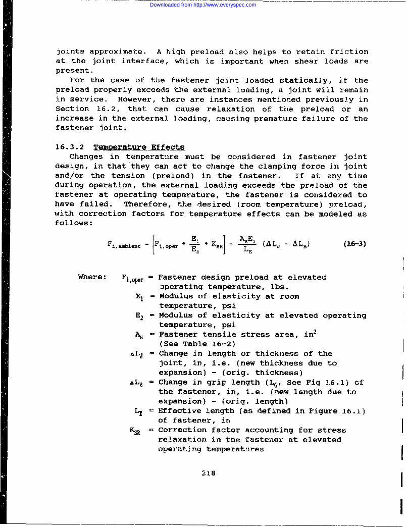
joints approximate. A high preload also helps to retain frictionat the joint interface, which is important when shear loads arepresent.

For the case of the fastener joint loaded statically, if thepreload properly exceeds the external loading, a joint will remainin service. However, there are instances mentioned previously inSection 16.2, that can cause relaxation of the preload or anincrease in the external loading, causing premature failure of thefastener joint.

16.3.2 TN=tre VZtaChanges in temperature must be considered in fastener joint

design, in that they can act to change the clamping force in jointand/or the tension (preload) in the fastener. If at any timeduring operation, the external loading exceeds the preload of thefastener at operating temperature, the fastener is conisidered tohave failed. Therefore, the desired (room temperature) preload,with correction factors for temperature effects can be modeled asfollows:

[E2 LEFiamint= t°Pr -•*Ksaj L (AL 0 - ALB) (16-3)

Where: Fi,or = Fastener design preload at elevatedoperating temperature, lbs.

El = Modulus of elasticity at roomtemperature, psi

E2= Modulus of elasticity at elevated operatingtemperature, psi

A= Fastener tensile stress area, in 2

(See Table 16-2)AU Change in length or thickness of the

joint, in, i.e. (new thickness due toexpansion) - (orig. thickness)

A LO= Change in grip length (LG, See Fig 3.6.1) ofthe fastener, in, i.e. (new length due toexpansion) - (orig. length)

LE =Effective length (as defined in Figure 16.1)of fastener, in

KSR Correction factor accounting for stressrelaxation in the fastener at elevatedoperating temperatures

218


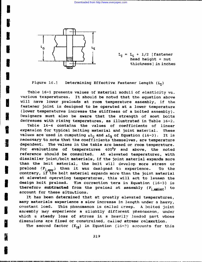
III

L LL = LG + 1/2 (fastener

head height + nutthickness ] in inches

IFigure 16.1 Determining Effective Fastener Length (LE)

I Table 16-i presents values of material moduli of elasticity vs.various temperatures. It should be noted that the equation aboveI will have lower preloads at room temperature assembly, if thefastener joint is designed to be operated at a lower temperature(lower temperatures increase the stiffness of a bolted assembly).Designers must also be aware that the strength of most boltsdecreases with rising temperatures, as illustrated in Table 16-2.

Table 16-4 contains the values of coefficients of linearexpansion for typical bolting material and joint material. Thesevalues are used in computing ALj and ALB of Equation (16-3). It isI necessary to note that the coefficients themselves, are temperaturedependent. The values in the table are based or room temperature.For evaluations of temperatures 400°F and above, the notedI reference should be consulted. At elevated temperatures, withdissimilar joint/bolt materials, if the joint material expands morethan the bolt material, the bolt will develop more stress or

I preload (Fi, 0X) than it was designed to experience. To thecontrary, if the bolt material expands more than the joint materialat elevated operating temperatures, this will act to lessen theU design bolt preload. The correction ter:m in Equation (.16-3) istherefore sudbtracted from the preload at assembly (Fil Wet) toaccount for these situations.

It has been determined that at greatly elevated temperatures,many materials experience a slow increase in length under a heavy,

I constant load. This phenomenon is called creep. A bolted jointas&.embly may experience a slightly different phenomceron, underwhich a steady loss of stress in a heavily i oia.ed part Vhhose

* dimensions are fixed or constrained,, called stress relaxiation.The second factor (K1u) in Equation (16-1) accounts for this

219

U


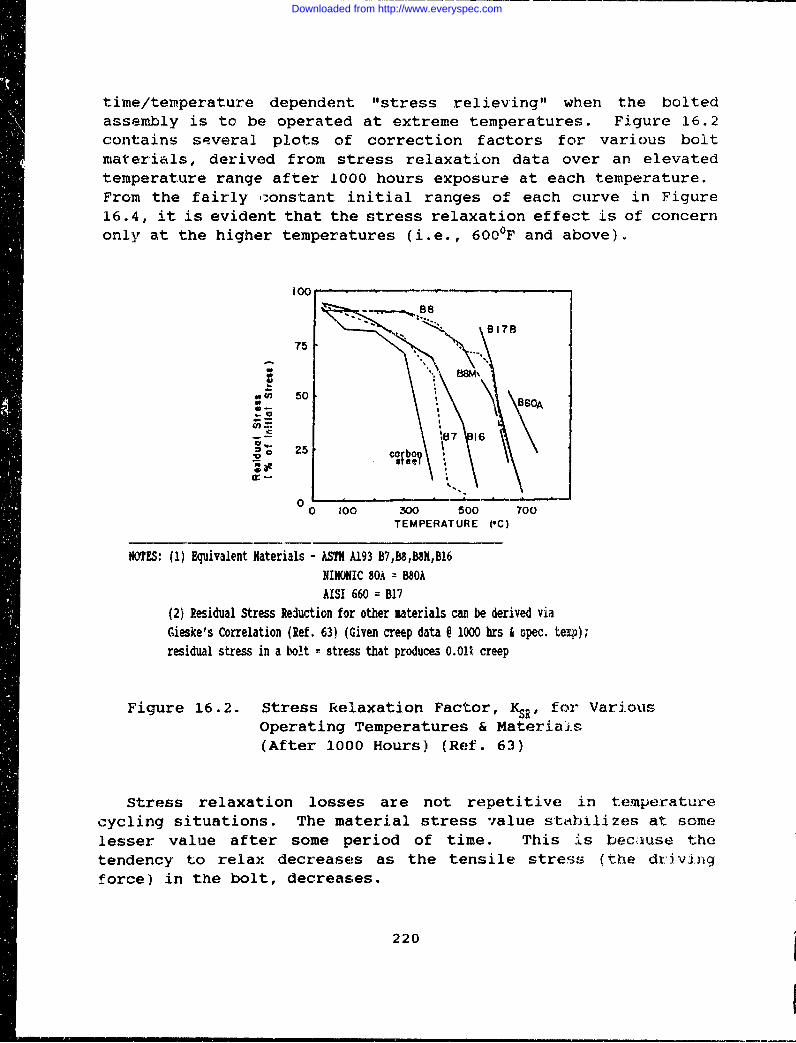
time/temperature dependent "stress relieving" when the boltedassembly is to be operated at extreme temperatures. Figure 16.2contains several plots of correction factors for various boltmaterials, derived from stress relaxation data over an elevatedtemperature range after 1000 hours exposure at each temperature.From the fairly .onstant initial ranges of each curve in Figure16.4, it is evident that the stress relaxation effect is of concernonly at the higher temperatures (i.e., 600OF and above).

100 SeBe

75 B

E18l

U) 50 880

-87 16_ 25 c 0rbo,

00 100 -00 500 700

TEMPERATURE ('C)

NOTES: (1) Equivalent Materials - ASTN A193 B7,B8,B8X,BI6NIMONIC 80A = B80AAISI 660 = B17

(2) Residual Stress Reduction for other aterials can be derived viaGieske's Correlation (Ref. 63) (Given creep data @ 1000 hrs & spec. temp);residual stress in a bolt = stress that produces 0.01T, creep

Figure 16.2. Stress Relaxation Factor, KSR' for VariousOperating Temperatures & Materials(After 1000 Hours) (Ref. 63)

Stress relaxation losses are not repetitive in temperaturecycling situations. The material stress value stabllizes at somelesser value after some period of time. This is because thetendency to relax decreases as the tensile stress (the drivingforce) in the bolt, decreases.

220


oo16.3.3 p eaCorrosion is a problem often faced when dealing with bolted

assemblies. Excessive corrosion can eventually lead to a reductionin preload, or to the total loss of clamping force throughdestruction of material. Several methods (Ref. 63) used to combatthe onset of corrosion are as follows:

1. Select materials in the joint assembly (bolts, nuts,structure) that are identical, or as close together as possible inthe galvanic series, minimiLing electrical potential differences.

"2. It is desirable, in a situation of dissimilar metals, to havethe larger amount of material present to act as an anode, while thesmaller amount of material behaves as the cathode.

3. Introduce a 'sacrificial' anode, that can be replaced fromI time to time. This can be a block of material placed in thevicinity of the bolted joint, where material is sacrificed in agalvanic reaction.

4. Minimize stresses and/or stress concentrations in fastenersand joints by providing generous fillets, polishing surtaces,preloading bolts uniformly, etc. Stress tends to mak.a a materialmore anodic. Therefore, stress concentrations at the root of acrack will make that portion of the bolt body more anodic, withrespect to the adjacunt portion; this aids in the growth of fatigue

f cracks.5. Various coatings can resist corrosion by -

(a) providing a barrier by isolating the bolt from thecorrosive environment,, Cadmium is a common coating,which provides barrier protection.

(b) inhibiting the process of corrosion.(c) prcvide galvanic/sacrificial protection of the anodic

material. Z inc-coated, or 'galvanized' fasteners providesacrificial protection,• along with some barrierprotection.

6. Periodic replacement of the xixlts, prior to failure, can bea practical solution. This approach intensif.ies the eed tbeable to accurat;elyy predict the amount of life remaining in afastener, so that the bolIted asslemblies are not distmantled5 prematurely.

Stress corrosion cracking is one of the more serious problems5 for bolting engineers. This if relatively common in many bolts,and may oltimately ead to sudden and unexpected failure (SeeFigure 16-3). Althoug.h every metal.ic. boltting material issusceptible to stress co G ci oir rackr i ng under certain conditions,

I ~2,21

I


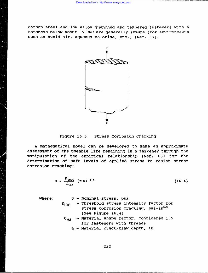
carbon steel and low alloy quenched and tempered fasteners with ahardness below about 35 HRC are generally immune (for environmentssuch as humid air, aqueous chloride, etc.) (Ref. 63).

F

Figure 16.3 Stress Corrosion Cracking

A mathematical model can be developed to make an approximateassessment of the useable life remaining in a fastener through themanipulation of the empirical relationship (Ref. 63) for thedetermination of safe levels of applied stress to resist stresscorrosion cracking:

a K15 cc (n a)o*- (16-4)

Where: a - Nominal stress, psiKI0 = Threshold stress intensity factor for

stress corrosion cracking, psi-inO. 5

(See Figure 16.4)CUW = Material shape factor, considered 1.5

for fasteners with thireadsa - Material crack/flaw depth, in

222


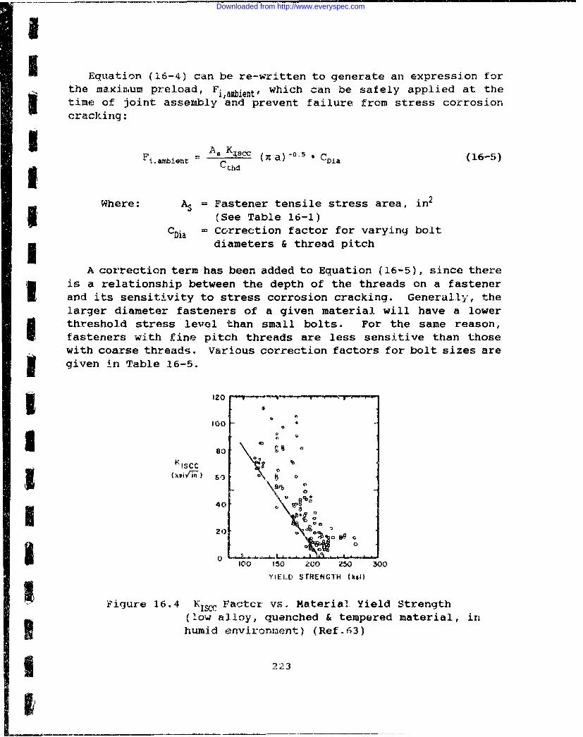
I

Equation (16-4) can be re-written to generate an expression fori the maximium preload, Fi,aabient, which can be safely applied at the

time of joint assembly and prevent failure from stress corrosioncracking:

F As 0iA8c Kscc (- a]- ia (16-5)

Cthd

Where: AS = Fastener tensile stress area, in 2

i (See Table 16-1)CDia = Correction factor for varying bolt

* diameters & thread pitch

A correction term has been added to Equation (16-5), since thereis a relationship between the depth of the threads on a fastenerand its sensitivity to stress corrosion cracking. Generally, thelarger diameter fasteners of a given material will have a lowerI threshold stress level than small bolts. For the same reason,fasteners with fine pitch threads are less sensitive than thosewith coarse threads. Various correction factors for bolt sizes areB I given in Table 16-5.

S~~~~~~~120O"r""

II

so 9

KISCC ,° %

40

20 to

5 °IOO 150 ZOO 250 300

YIELD STRENGTH (kWl)

Figure 16.4 KISCr Facter vs. Material Yield Strength(low alloy, quenched & tempered material, inhumid environnent) (Ref .3)

223I "2


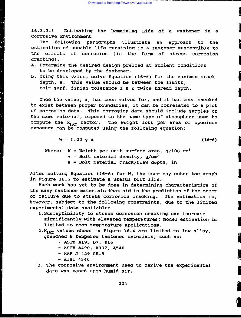
16.3.3.1 Estimating the Remaining Life of a Fastener in aCorrosive Environment

The following paragraphs illustrate an approach to theestimation of useable life remaining in a fastener susceptible tothe effects of corrosion (in the form of stress corrosioncracking).A. Determine the desired design preload at ambient conditions

to be developed by the fastener.B. Using this value, solve Equation (16-5) for the maximum crack

depth, a. This value should be between the limits,bolt surf. finish tolerance : a Ž twice thread depth.

Once the value, a, has been solved for, and it has been checkedto exist between proper boundaries, it can be correlated to a plotof corrosion data. This corrosion data should include samples ofthe same material, exposed to the same type of atmosphere used tocompute the KISCC factor. The weight loss per area of specimenexposure can be computed using the following equation:

W = 0.03 y a (16-6)

Where: W = Weight per unit surface area, g/100 cm2

y = Bolt material density, g/cm3

a = Bolt material crack/flaw depth, in

After solving Equation (16-6) for W, the user may enter the graphin Figure 16.5 to estimate a useful bolt life.

Much work has yet to be done in determining characteristics ofthe many fastener materials that aid in the prediction of the onsetof failure due to stress corrosion cracking. The estimation is,however, subject to the following constraints, due to the limitedexperimental data available:

l.Susceptibility to stress corrosion cracking can increasesignificantly with elevated temperatures; model estimation islimited to room temperature applications.

2.K,,, values shown in Figure 16.4 are limited to low alloy,quenched & tempered fastener materials, such as:

- ASTM A193 B7, B16- ASTM A490, A307, A540- SAE J 429 GR.8- AISI 4340

3. The corrosive environment used to derive the experimentaldata was based upon humid air.

224


I£12 7

)0 10

I II

tpI

3o -3 4 5 - 6

Time, yearsI Figure 16.5 Typical Coupon Corrosion PenetrationTest Results, (Low alloy steel in humid

6 air) (Ref. 64)

416.3.4 Dyn7/ic Loading

I Machinery in operation is a dynamic situation. For the mostpart then, fasteners used in many applications have a small dynamic

I load superimposed on a much larger static prelcad. These dynamicor 'fluctuating" loads are augmented by stress concentrations andbending.I 16.3.5 Determination of Base Failure Rate

Data available from fastener manufacturers that have performed

I extensive testing, can be used to determine the base failure rate,MacHowever, since this data is somewhat specific to the

S conditions or environment of the test, it is often difficult tolocate data that will yieldhthe base failure rate of a specific

type of fastener, under a particular set of loading conditions.i This necessitates the development of a procedure to estimate the

base failure rate of a generic fastener, with variouscharacteristics and loading conditions.

Fatigue, as discussed in Section 16.2, can limit the useable

life of a fastener in a dynamic loading condition. Fatigue limit

testing can be valuable in developing a model for fastener failureI rates. A large number of tests are necessary to establish the

fatigue strength of a material due to the statistical nature of

3 225

I


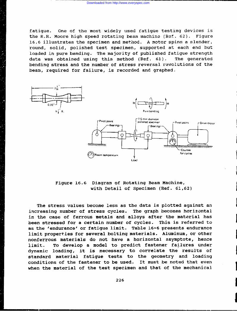
fatigue. One of the most widely used fatigue testing devices isthe R.R. Moore high speed rotating beam machine (Ref. 62). Figure16.6 illustrates the specimen and method. A motor spins a slender,round, solid, polished test specimen, supported at each end butloaded in pure bending. The majority of published fatigue strengthdata was obtained using this method (Ref. 61). The generatedbending stress and the number of stress reversal revolutions of thebeam, required for failure, is recorded and graphed.

16 3

9' R. Pure bending

7.5 mm diameterPivot point polished specimen Pivot point Drive motor

Bearings -Bearongs

Room temperature. for cycles

Load

Figure 16.6 Diagram of Rotating Beam Machine,with Detail of Specimen (Ref. 61,62)

The stress values become less as the data is plotted against anincreasing number of stress cycles. The graph becomes horizontalin the case of ferrous metals and alloys after the material hasbeen stressed for a certain number of cycles. This is referred toas the 'endurance' or fatigue limit. Table 16-6 presents endurancelimit properties for several bolting materials. Aluminum, or othernonferrous materials do not have a horizontal asymptote, hencelimit. To develop a model to predict fastener failures underdynamic loading, it is necessary to correlate the results ofstandard material fatigue tests to the geometry and loadingconditions of the fastener to be used. It must be noted that evenwhen the material of the test specimen and that of the mechanical

226


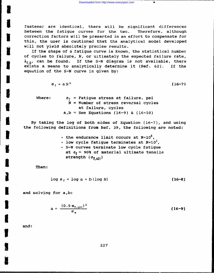
I fastener are identical, there will be significant differencesbetween the fatigue curves for the two. Therefore, althoughcorrection factors will be presented in an effort to compensate forthis, the user is cautioned that the analytical model developedwill not yield absolutely precise results.

If the shape of a fatigue curve is known, the statistical numberof cycles to failure, N, or ultimately the expected failure rate,

IF,B, Ican be found. If the S-N diagram is not available, thereexists a means to analytically determine it (Ref. 62). If theequation of the S-N curve is given by:

U of = aNb (16-7)

I Where: of = Fatigue stress at failure, psiN = Number of stress reversal cycles

at failure, cyclesa,b = See Equations (16-9) & (16-10)

£ By taking the log of both sides of Equation (16-7), and usingthe following definitions from Ref. 39, the following are noted:

I • the endurance limit cccurs at N=10 6,• low cycle fatigue terminates at N=10 3,

• S-N curves terminate low cycle fatigueat of = 90% of material ultimate tensilestrength (OT,ult)

Then:

I log of = log a + b(log N) (16-8)

ft and solving for a,b:

a (0.9 =TUlt (16-9)aeI

and:

23 227

1


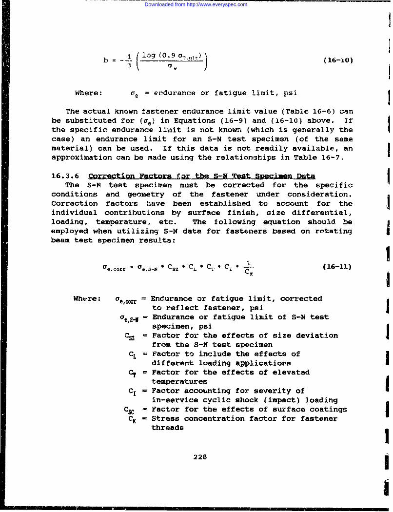
b 1(log (0.9)0"'tb (16-10)

Where: ce = endurance or fatigue limit, psi

The actual known fastener endurance limit value (Table 16-6) canbe substituted for (ae) in Equations (16-9) and (16-10) above. Ifthe specific endurance limnit is not known (which is generally thecase) an endurance limit for an S-N test specimen (of the samematerial) can be used. If this data is not readily available, anapproximation can be made using the relationships in Table 16-7.

16.*3.*6 Corretion Factors iar Ih S-Nes SW ce .Datm IThe S-N test specimen must be corrected for the specific

conditions and geometry of the fastener under consideration.Correction factors have been established to account for theindividual contributions by surface finish, size differential,loading, temperature, etc. The following equation should beemployed when utilizing S-N data for fasteners based on rotatingbeam test specimen results:

aelcozz = O,_ * Csz * CL 0 CT 1 Cz * (16-11) 1cxI

Where: =e,cor= Endurance or fatigue limit, correctedto reflect fastener, psi

Ge,S.= Endurance or fatigue limit of S-N testspecimen, psi

CSZ= Factor for the effects of size deviationfrom the S-N test specimen

CL Factor to include the effects ofdifferent loading applications

C= Factor for the effects of elevatedtemperatures

C1 = Factor accounting for severity ofin-service cyclic shock (impact) loading

Cs = Factor for the effects of surface coatingsCK= Stress concentration factor for fastener

threads

228


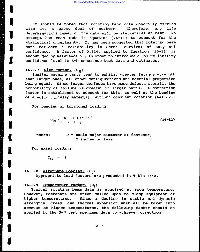
SI It should be noted that rotating beam data generally carrieswith it, a great deal of scatter. Therefore, any life

I determinations based on the data will be statistical at best. Noattempt has been made in Equation (16-11) to account for thestatistical uncertainty. It has been suggested that rotating beamdata reflects a reliability in actual survival of only 50%confidence. A factor of 0.814, applied to Equation (16-12) isencouraged by Reference 61, in order to introduce a 99% reliabilityconfidence level in S-'N endurance test data and estimates.

16.3.7 SiZVe Fact, (Csz)I Smaller machine parts tend to exhibit greater fatigue strengththan larger ones, all other configurations and material propertiesbeing equal. Since larger surfaces have more defects overall, theprobability of failure is greater in larger parts. A correctionfactor is established to account for this, as well as the bendingof a solid circular material, without constant rotation (Ref 62):

For bending or torsional loading:

0= -0 (16-13)

Where: D - Basic major diameter of fastener,I 2 inches or less

3 IFor axial loading:

C = 1

16.3.8 Alternate ding,- (CL)Appropriate load factors are presented in Table 16-8.

16.3.9 Texperature Factor. (CT)i Typical rotating beam data is acquired at room temperature.However, fasteners are often called upon to clamp equipment athigher temperatures. Since a decline in static and dynamicU strengths, creep, and thermal expansion must all be taken intoaccount at higher temperatures, the following factor should beapplied to the S-N test specimen data to achieve correction:

3 229


For s operating above 160°F:

CT 620 (16-14)(460 + Tope)

Where: 10m = operating temperature of fastener, F

16.3.10 Cyclic Shock/Ipmact Loading. (Cl)A correction factor must be applied when shock loads are

present. In general, cyclic loads are less severe than appliedshock loading. The factors are presented in Table 16-9.

16.3.11 Surface CoatingS. (Cx)Surface treatments such as electroplating and spraying act to

reduce the endurance limit. If any of these operations are to beused, Table 16-10 provides the correction factors.

16.3.12 Thread Correction Faor,.-. (CK)

Observations of typical bolt failure pattern data from Ref. 62have revealed that only about 15% of failures occur under the head,due to the stress riser caused by the fillet. The risers found inthe thread area accounted for the other 85%. Therefore, Table 16-11 presents the correction factor for stress risers caused by theintroduction of threads. The effects of notch sensitivity andsurface finish have been incorporated.

230


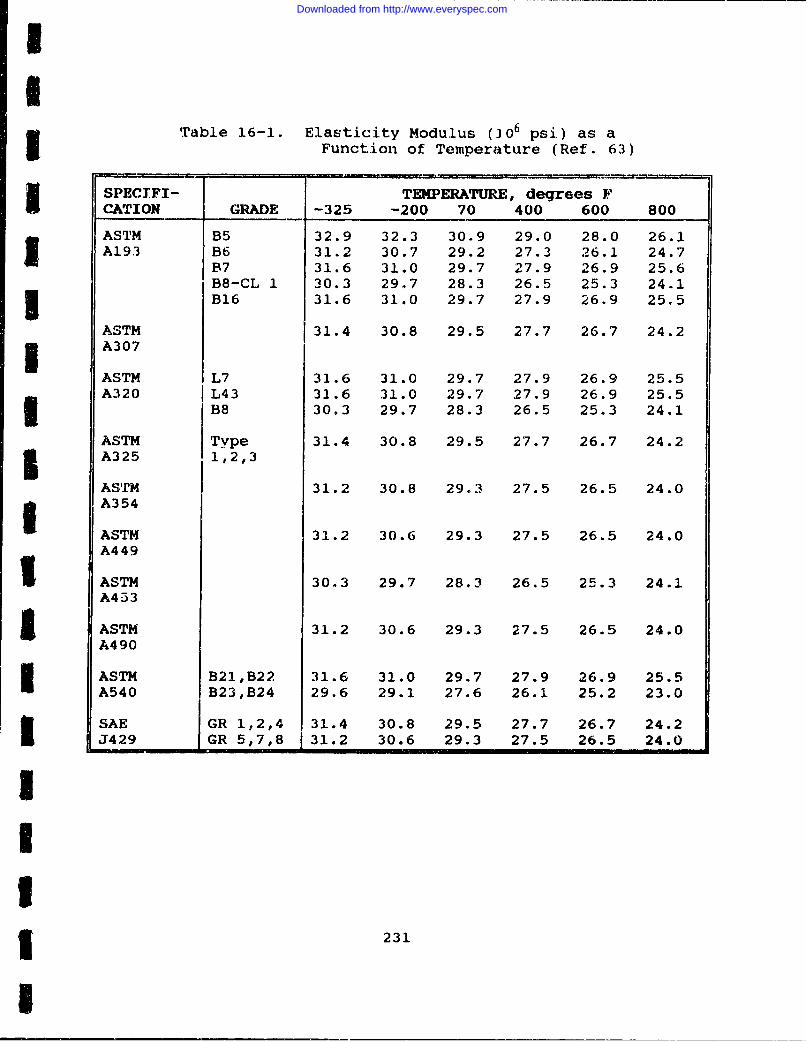
3I

Table 16-1. Elasticity Modulus (306 psi) as aFunction of Temperature (Ref. 63)

SPECIFI- TEMPERATURE, degrees FCATION GRADE -325 -200 70 400 600 800

ASTM B5 32.9 32.3 30.9 29.0 28.0 26.1A193 B6 31.2 30.7 29.2 27.3 26.1 24.7

B7 31.6 31.0 29.7 27.9 26.9 25.6B8-CL 1 30.3 29.7 28.3 26.5 25.3 24.1B16 31.6 31.0 29.7 27.9 26.9 25.5

ASTM 31.4 30.8 29.5 27.7 26.7 24.23 A307

ASTM L7 31.6 31.0 29.7 27.9 26.9 25.5A320 L43 31.6 31.0 29.7 27.9 26.9 25.5

B8 30.3 29.7 28.3 26.5 25.3 24.1

ASTM Type 31.4 30.8 29.5 27.7 26.7 24.2I A325 1,2,3

ASTM 31.2 30.8 29.3 27.5 26.5 24.0A354

ASTM 31.2 30.6 29.3 27.5 26.5 24.0A4 49

A4ASTM 30.3 29.7 28.3 26.5 25.3 24.1A453

I ASTM 31.2 30.6 29.3 27.5 26.5 24.0A490

ASTM B21,B22 31.6 31.0 29.7 27.9 26.9 25.5A540 B23,B24 29.6 29.1 27.6 26.1 25.2 23.0

SAE GR 1.,2,4 31.4 30.8 29.5 27.7 26.7 24.2J429 GR 5,7,8 31.2 30.6 29.3 27.5 26.5 24.0

231II

3 231

1


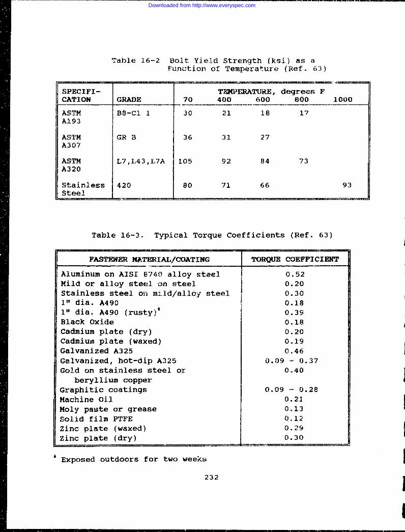
Table 16-2 Bolt Yield Strength (ksi) as aFunction of Temperature (Ref. 63)

SPECIFI- TWPEFRATU"i., degrees FCATION GRADE 70 400 600 800 1000

ASTM B8-C1 1. 30 21 18 17A193

ASTM GR B 36 31 27A307

ASTM L7,L43,L7A 105 92 84 73A320

Stainless 420 80 71 66 93Steel

Table 16-3. Typical Torque Coefficients (Ref. 63)

FASTENER MATERIAL/COATING TORQUE COEFFICIENT

Aluminum on AISI 8740 alloy steel 0.52Mild or alloy steel on steel 0.20Stainless steel on mild/alloy steel 0.301" dia. A490 0.181" dia. A490 (rusty)* 0.39Black Oxide 0.18Cadmium plate (dry) 0.20Cadmium plate (waxed) 0.19Galvanized A325 0.46Galvanized, hot-dip A325 0.09 - 0.37Gold on stainless steel or 0.40

beryllium copperGraphitic coatings 0.09 - 0.28Machine Oil 0.21Moly paste or grease 0.13Solid film PTFE 0.12Zinc plate (waxed) 0.29Zinc plate (dry) 0.30

Exposed outdoors for two weeks

232


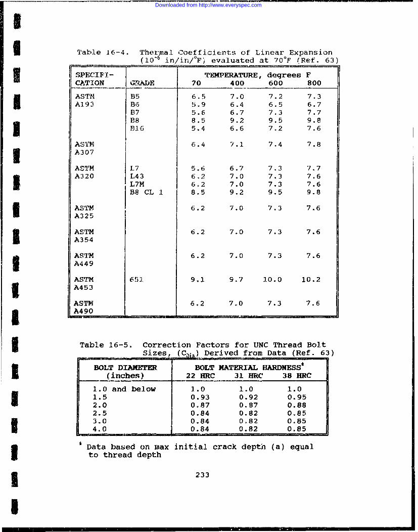
I

Table 16-4. Thermal Coefficients of Linear Expansion(10-6 in/in/F:i evaluated at 70 0 F (Ref. 63)

3 ECIF1.- ITEMPERATURE, degrees FCATION GPhDE 70 400 600 800

ASTM B5 6.5 7.0 7.2 7.3A193 B6 5.9 6.4 6.5 6.7

B7 5.6 6.7 7.3 7.7B8 8.5 9.2 9.5 9.8B16 5.4 6.6 7.2 7.6

ASTM 6.4 7.1 7.4 7.83 A307

ASTM L7 5.6 6.7 7.3 7.7A320 L43 6.2 7.0 7.3 7.6

I L7M 6.2 7.0 7.3 7.6B8 CL 1 8.5 9.2 9.5 9.8

ASTM 6.2 7.0 7.3 7.6A325

ASTM 6.2 7.0 7.3 7.6A354

ASTM 6.2 7.0 7.3 7.6A449

ASTM 651 9.1 9.7 10.0 10.2A453

ASTM 6.2 7.0 7.3 7.6SA490 1 1

Table 16-5. Correction Factors for UNC Thread Bolt

Sizes, (Ci) Derived from Data (Ref. 63)

BOLT DIAMETER BOLT MATERIAL HARDNESS'(inches) 22 HRC 31 HRC 38 HRC

1.0 and below 1.0 1.0 1.01.5 0.93 0.92 0.952.0 0.87 0.87 0.882.5 0.84 0.82 0.853.0 0.84 0.82 0.854.0 0.84 0.82 0.85

* Data based on imax initial crack depth (a) equalto thread depth

3 233

I


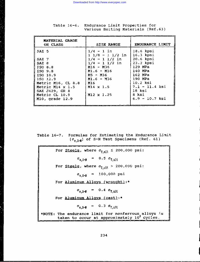
Table J.6-6. Endurance Limit Properties forVarious Bolting Materials (Ref.63)

MATERIAL GRADEOR CLASS SIZE RANGE ENDURANCE LIMIT

SAE 5 1/4 - 1 in 18.6 kpsi1 1/8 - 1 1/2 in 16.3 kpsi

SAE 7 1/4 - 1 1/2 in 20.6 kpsiSAE 8 1/4 - 1 1/2 in 23.2 kpsiISO 8.8 M16 - M36 129 MPaISO 9.8 M1.6 - M16 140 MPaISO 10.9 M5 - M36 162 MPaISo 12.9 M1.6 - M36 190 MPaMetric M16, CL 8.8 M16 10.2 ksiMetric M14 x 1.5 M14 x 1.5 7.1 - 11.4 ksiSAE J429, GR 8 18 ksiMetric CL 10.9 M12 x 1.25 8 ksiM10, grade 12.9 6.9 - 10.7 ksi

Table 16-7. Formulas for Estimating the Endurance Limit(Oe,SN) of S-N Test Specimens (Ref. 61)

For S , where aT,at : 200,000 psi:

e,S.N 0.5 OTult

For ateelj;, where aT,ult > 200,000 psi:

oes.N= 0,0•000 psi

For A•luminum Alloywnt~il:*

ae,S.-= 0.4 aT,ult

For Aluminum Alloys (-jAS•a:*

ae,S.N - 0.3 cT,ult

*NOTE: The endurance limit for nonferrous alloys istaken to occur at approximately 108 cycles

234


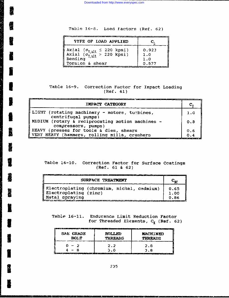
Table 16-83. Load Factors (Ref. 62)

3 -TYPE OF L)AD APPLIED CL

Axial (aT,ut 220 kpsi) 0.923Axial (aT ult > 220 kpsi) 1.0

SBending 1.0Torsion & shear 0.577

3 Table 16-9. Correction Factor for Impact Loading(Ref. 61)

IMPACT CATEGORY C1

LIGHT (rotating machinerj - motors, turbines, 1.0I centrifugal pumps)MEDIUM (rotary & reciprocating motion machines - 0.8

compressors, pumps)z HEAVY (presses for tools & dies, shears 0.6

VERY HEAVY (hammers, rolling mills, crushers 0.4

II Table 16-10. Correction Factor for Surface Coatings

(Ref. 61 & 62)

ISURFACE TREATMENTCCElectroplating (chromium, nickel, cadmium) 0.65

w Electroplating (zinc) 1.00Metal spraying ___"0.86

ITable 3.6-i.1. Endurance Limit Reduction Factor3 for Threaded Elements, C, (Ref. 62)

SAE G'RADE ROLLED MACH.INED0 - 2 2.2 2.8~4 -8 3.0 3.8

1 2 25

I



236


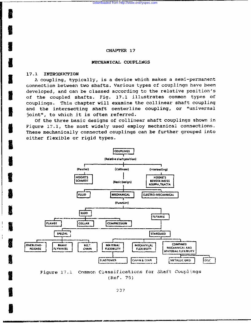
II

I CHAPTER 17

j MECHANICAL COUPLINGS

I 17.1 INTRODUCTIONA coupling, typically, is a device which makes a semi-permanent

connection between two shafts. Various types of couplings have beendeveloped, and can be classed according to the relative position'sof the coupled shafts. Fig. 17.1 illustrates common types ofcouplings. This chapter will examine the collinear shaft couplingI and the intersecting shaft centerline coupling, or "universaljoint", to which it is often referred.

Of the three basic designs of collinear shaft couplings shown inI Figure 17.1, the most widely used employ mechanical connections.

These mechanically connected couplings can be further grouped intoeither flexible or rigid types.

I ~NGS

(Relative s•aft position)

(Parellel) (Collinear) (Intersecting)

HOOKE'S IHOOKE'SSCHIDT(Basic Design) IENOIX-WEISS

ffI #HAIL ELCTOMECNICAL(Function)

C7[OLLLAR COMRESSION]

OVROD-U~iAJK 1 ] E MAT~RA MECHIANICAL r COMnUNFDRELEASE FYWHEEL I CHAIN I FLEXJIIY rLEX181urT MECHANICAL AND

[ELASTOMER J~ CaWL kTrLL ~

Figure 1`7.1 Common ClassiAItcatioxt for 3haft, Coup.1;,ngs

(Ref. 75)

i 2373|?3


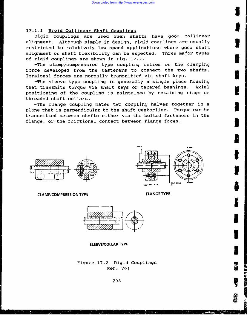
U

17.1.1 agid Collinear Shaft CouplingsRigid couplings are used when shafts have good collinear

alignment. Although simple in design, rigid couplings are usuallyrestricted to relatively low speed applications where good shaftalignment or shaft flexibility can be expected. Three major typesof rigid couplings are shown in Fig. 17.2. 5

-The clamp/compression type coupling relies on the clampingforce developed from the fasteners to connect the two shafts.Torsional forces are normally transmitted via shaft keys. I

-The sleeve type coupling is generally a single piece housingthat transmits torque via shaft keys or tapered bushings. Axialpositioning of the coupling is maintained by retaining rings or Ithreaded shaft collars.

-The flange coupling mates two coupling halves together in aplane that is perpendicular to the shaft centerline. Torque can be Itransmitted between shafts either via the bolted fasteners in theflange, or the frictional contact between flange faces. i

I

SECTIO A-A PAA

CLAMP/COMPRESSION TYPE FLANGE TYPE

SLEEVE/COLLAR TYPE

Figure 17.2 Rigid CouplingsRef. 76)

238 +;1


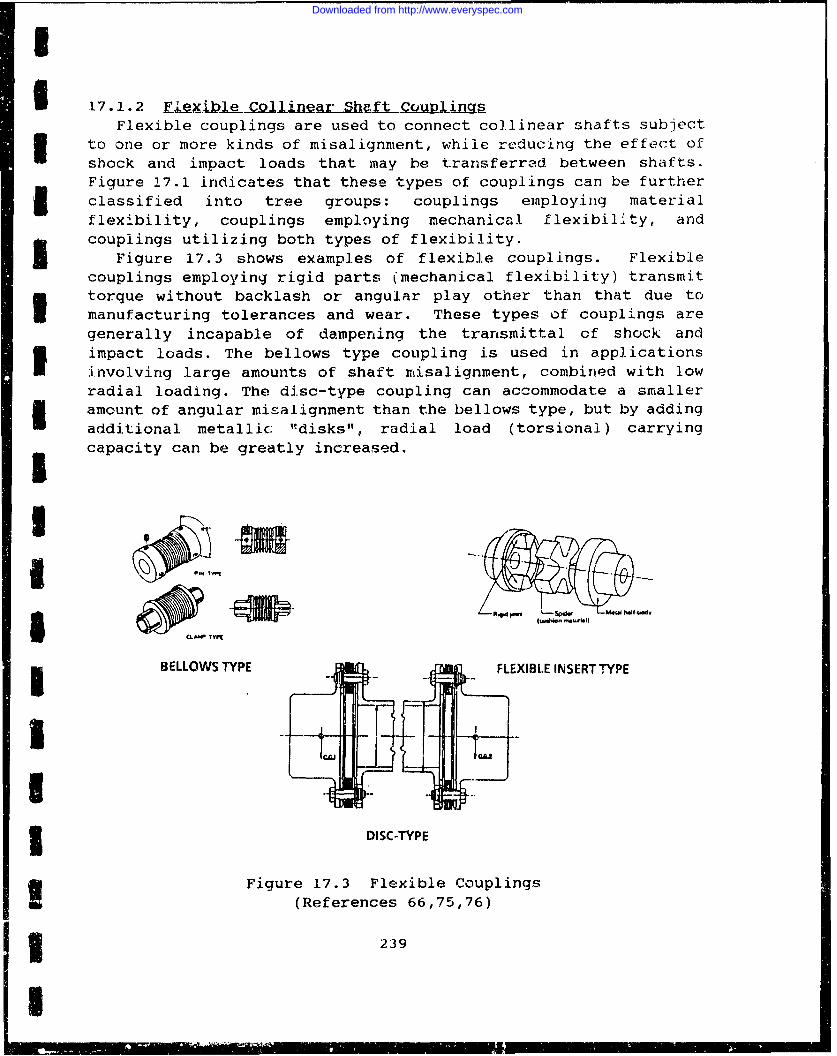
I

Flexible couplings are used to connect collinear shafts subjectI to one or more kinds of misalignment, while reducing the effect of

shock and impact loads that may be transferred. between shafts.Figure 17.1 indicates that these types of couplings can be furtherclassified into tree groups: couplings employing materialflexibility, couplings employing mechanical flexibility, andcouplings utilizing both types of flexibility.

Figure 17.3 shows examples of flexible couplings. Flexiblecouplings employing rigid parts (mechanical flexibility) transmit

I torque without backlash or angular play other than that due tomanufacturing tolerances and wear. These types of couplings aregenerally incapable of dampening the transmittal of shock and

I impact loads. The bellows type coupling is used in applicationsinvolving large amounts of shaft misalignment, combined with lowradial loading. The disc-type coupling can accommodate a smallerI amount of angular misalignment than the bellows type, but by addingadditional metallic. "disks", radial load (torsional) carryingcapacity can be greatly increased.

I£,,T"M h--+o

BELLOWS TYPE FLEXIBLE INSERTTYPE

I

3 DISC-TYPE

Figure 17.3 Flexible Couplings(References 66,75,76)

1 239

I


Flexible couplings containing resilient components (material

flexibility) can accommodate shaft misalignment, as well as dampen

shock and impact loads. This type of coupling possesses torsional

flexibility, often acting as "detuning" devices by altering thevibration properties of the connected system. The flexible inserttype coupling shown in Figure 17.3 transmits torque through an oil jresistant rubber spider assembled between two pairs of axiallyoverlapping rigid jaws.

Examples of the third type of flexible coupling type (materialand mechanical flexibility) are the metallic grid and the diaphragmcoupling. The metallic grid coupling consists of two metal half-bodies with slots cut into the peripheries to seat a serpent like Ispring steel alloy grid. The deflection of the springs under loadhelp to reduce shock loading, thereby utilizing the bestcharacteristics of material and mecharnical coupling flexibilities. I

Table 17-1 indicates the range of performance characteristicspossible with flexible couplings. Due to the varying ranges ofperformance, it is easy to see why some caution must be taken inselecting the correct coupling for the operating conditions to beencountered. Diaphragm couplings are rated for high speedoperation, but accept only a small amount of misalignment.Although elastomeric and gear type couplings can accommodate a fairamount of angular misalignment, in general, the gear coupling israted to accept heavier duty (horsepower). Again, a tradeoff mustmade, since gear couplings require periodic maintenance in thereplenishment of lubrication and seals.

A representative graphic comparison of flexible coupling typesis sr..wn in Figure 17.4. Figure 17.4(a) shows the clearsuperiority of an elastomeric material flexible coupling over theother two types when angular and parallel shaft misalignments areexcessive. However, the mechanical flexibility of the disk-type ormetallic grid can carry a much greater load at smaller degrees ofshaft misalignment. This is illustrated in Figure 17.4(b).

17.2 FAILURE MODES OF FLEXIBLE COUPLINGSTable 17.2 lists various failure modes encountered when using

flexible couplings. Many of these failures can be avoided byproperly selecting the correct type, size and rating for theintended operational environment.

Coupling reliability is affected by the method used to mount thecoupling hub on the shafts of connected qquipment. The preferredprocedure is to use an interference fit between hub and shaft ofapproximately 0.005 inches per inch of shaft diameter. Although

240

S• • 'I! •q' r•!" P' P•' '• ,• I " ,• ,•- • w l l~ 1, • ' ,i ii


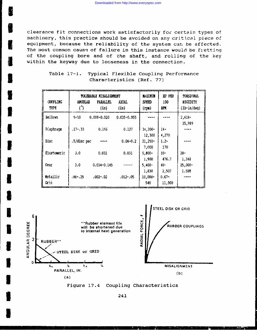
I

I clearance fit connections work satisfactorily for certain types otmachinery, this practice should be avoided on any critical piece ofequipment, because the reliability of the system car, be affected.The most common cause of failure in this instance would be frettingof the coupling bore and of the shaft, and rolling of the keywithin the keyway due to looseness in the connection.

Table 17-1. Typical Flexible Coupling PerformanceCharacteristics (Ref. 77)

TOLERABLE NISALIGNIENT NAXIIUN HP PER TRSI)NAL(XOPLING ANGULAR PARALLEL AXIAL SPEED 100 RIGIDITY3 TYPE (C) (in) (in) (rpm) RPPM (Ib-in/deg)

Bellows 5-10 0.008-0.010 0.035-0.055 ---- 2,618-

35,989Diaphrdqam .17-.33 0.166 0.127 34,300- 14- ----

12,300 4,270Disc .5/disc pac ---- 0.06-0.2 21,250- 1.2-

7,000 170Elastomeric 3.0 0.031 0M031 5,800- 10- 28-

I 1,900 476.7 1,348Gear 3.0 0.034-0,145 5,400- 40- 25,000-

1,830 2,507 1.58MMetallic .06-.25 .002-.02 .012-.05 10,000- 0.67-Grid 540 11,900

ISTEEL DISK OR GRID

16 U""Rubber element llfe Q"f will be shortened due Oto internal heat generation u.

'- RUBBER**

z .-STEEL DISK or GRIDz

4. Y/, 6 V. MISALIGNMENTPARALLEL, IN.(b)

i ~(a)()

Figure 17.4 Coupling Characteristics

3 241

U


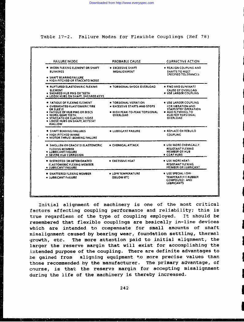
Table 17-2. Failure Modes for Flexible Couplings (Ref 78)

FAILURE MODE PROBABLE CAUSE CORRECrIVE ACTION

l WORN FLEXING ELEMENT OR SHAFT 0 EXCESSIVE SHAFT * REALIGN COUPLING ANDBUSHINGS MISALIGNMENT SHAFTS TO MEET

SPECIFIED TOLERANCES• SHAFT BEARING FAILURE* HIGH-PITCHED OR STACCATO NOISE

• RUPTURED ELASTOMERIC FLEXING 0 TORSIONAL SHOCK OVERLOAD 9 FIND AND ELIMINATFELEMENT CAUSE OF OVEIRLGAD

* SHEARED HUB PINS OR TEETH * USE LARGER COUPLING* LOOSE HUBS ON SHAFT, SHEARED KEYS

0 FATIGUE OF FLEXING ELEMENT e TORSIONAL VIBRATION a USE LARGER COUPLING"• OVERHEATED ELASTOMERIC TIRE v EXCESSIVE STARTS AND STOPS ICR VIBRATION AND

OR SLEEVE START/STOP OPERATION"* FATIGUE OF HUB PINS OR DISCS a HIGH PEAK-TO-PEAKTORSIONAL * ADDFLYWHEELTO"* WORK, GEAR TEETH OVERLOAD HUB FOR TORSIONAL"* STACCATO OR CLACKINC NOISE OVERLOAD"* LOOSE HUBS ON SHAFT, KEYSEAT

WALLOW

* SHAFT BEARING FAILURES • LUBRICANT FAILURE * REPLACE OR REBUILD* HIGH-PITCHED WHINE COUPLINGa MOTOR THRUS) BEARING FAILURE

* SWOLLEN OR CRACK!D ELASTOM:RIC • CHEMICALATTACK 0 USE MORE CHEMICALLY

FLEXING MI-MBER RESISTANT FLEXING• LUBRICANT FAILURE MEMBER OR HUB* SEVERE HUE CORROSION o COAT HUBS

* DISTROTED OR DETERIORATED * EXCESSIVE HEAT o USE MORE HEAT-ELASTOMERIC FLEXING MEMBER RESISTANT FLEXING

* LUBRICANT FAILURE MEMBER OR LUBRICANT

* SHATTERED FLEXING MEMBER e LOW TEMPERATURE * USE SPECIAL LOW-

* LUBRICANT FAILURE (BELOW OF) TEMPERATUI E RUBBERCOMPOUND'S., ANDLUBRICANTS

Initial alignment of machinery is one of the most criticalfactors affecting coupling performance and reliability; this istrue regardless of the type of coupling employed. It should beremembered that flexible couplings are basically in-line deviceswhich are intended to compensate for small amounts of shaftmisalignment caused by bearing wear, foundation settling, thermalgrowth, etc. The more attention paid to initial alignment, thelarger the reserve margin that will exist for accomplishing theintended purpose of the coupling. There are definite advantages tobe gained from aligning equipment to more precise values thanthose recommended by the manufacturer. The primary advantage, ofcourse, is that the reserv3 margin for accepting misalignmentduring the life of the machinery is thereby increased.

242

"': ]' • '! s" "!•' I I I ' I • = i n •1 r ] I :I


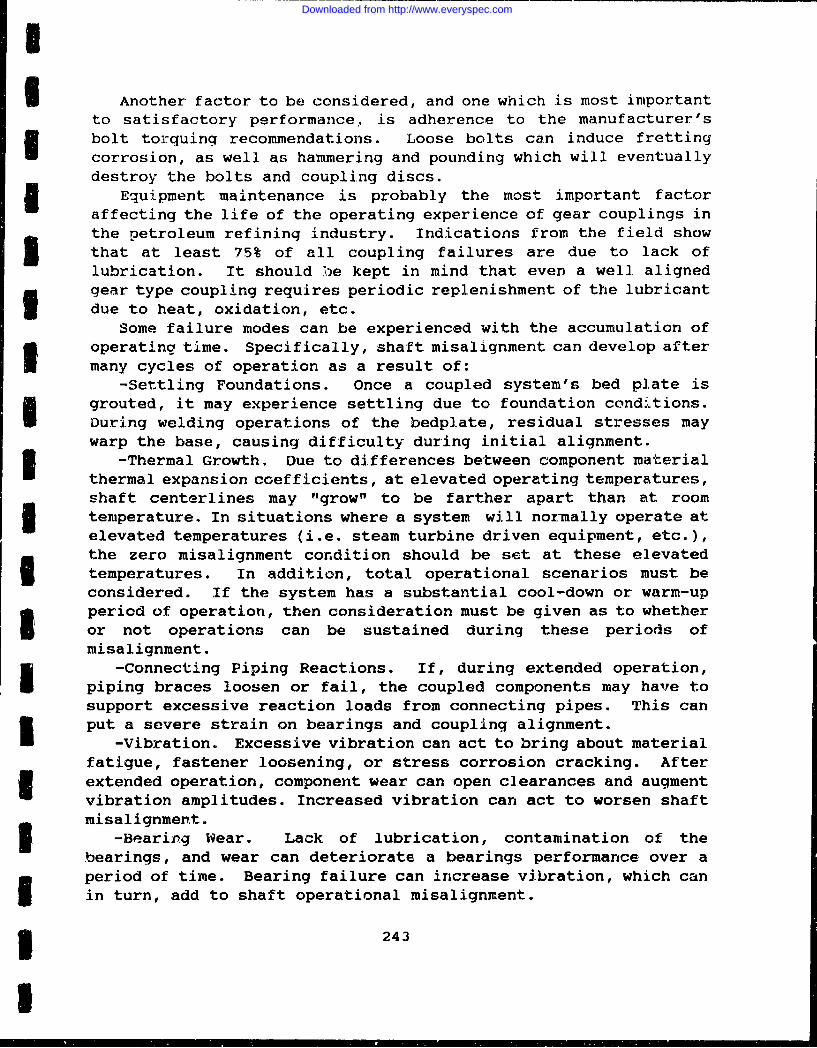
I Another factor to be considered, and one which is most importantto satisfactory performance, is adherence to the manufacturer'sbolt torquing recommendations. Loose bolts can induce frettingcorrosion, as well as hammering and pounding which will eventuallydestroy the bolts and coupling discs.

Equipment maintenance is probably the most important factoraffecting the life of the operating experience of gear couplings inthe petroleum refining industry. Indications from the field showthat at least 75% of all coupling failures are due to lack oflubrication. It should be kept in mind that even a well alignedgear type coupling requires periodic replenishment of the lubricantdue to heat, oxidation, etc.

Some failure modes can be experienced with the accumulation ofI operatinq time. Specifically, shaft misalignment can develop after

many cycles of operation as a result of:-Settling Foundations. Once a coupled system's bed plate is

grouted, it may experience settling due to foundation conditions.During welding operations of the bedplate, residual stresses maywarp the base, causing difficulty during initial alignment.

-Thermal Growth. Due to differences between component materialthermal expansion coefficients, at elevated operating temperatures,shaft centerlines may "grow" to be farther apart than at room

S temperature. In situations where a system will normally operate atelevated temperatures (i.e. steam turbine driven equipment, etc.),the zero misalignment condition should be set at these elevatedtemperatures. In addition, total operational scenarios must beconsidered. If the system has a substantial cool-down or warm-upperiod of operation, then consideration must be given as to whetheror not operations can be sustained during these periods ofmisalignment.

-Connecting Piping Reactions. If, during extended operation,piping braces loosen or fail, the coupled components may have tosupport excessive reaction loads from connecting pipes. This canput a severe strain on bearings and coupling alignment.

-Vibration. Excessive vibration can act to bring about materialfatigue, fastener loosening, or stress corrosion cracking. Afterextended operation, component wear can open clearances and augmentvibration amplitudes. Increased vibration can act to worsen shaftmisalignment.3 -Bearing Wear. Lack of lubrication, contamination of thebearings, and wear can deteriorate a bearings performance over aperiod of time. Bearing failure can increase vibration, which canin turn, add to shaft operational misalignment.

3 243

I


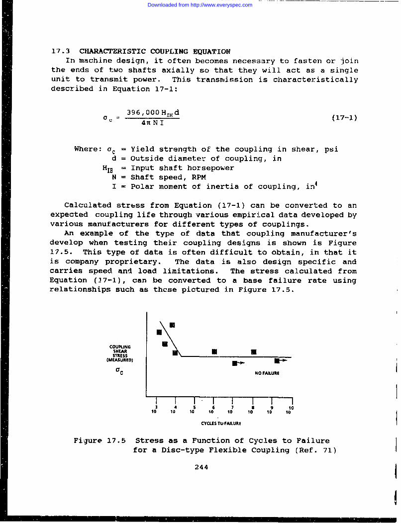
17.3 CHARACTERISTIC COUPLING EQUATIONIn machine design, it often becomes necessary to fasten or join

the ends of two shafts axially so that they will act as a singleunit to transmit power. This transmission is characteristicallydescribed in Equation 17-1:

396,000 HIH d (17-1)47t N I

Where: c= Yield strength of the coupling in shear, psid = Outside diameter of coupling, in

HIH = Input shaft horsepowerN = Shaft speed, RPMI = Polar moment of inertia of coupling, in4

Calculated strbss from Equation (17-1) can be converted to anexpected coupling life through various empirical data developed byvarious manufacturers for different types of couplings.

An example of the type of data that coupling manufacturer'sdevelop when testing their coupling designs is shown is Figure17.5. This type of data is often difficult to obtain, in that itis company proprietary. The data is also design specific andcarries speed and load limitations. The stress calculated fromEquation (27-1), can be converted to a base failure rate usingrelationships such as thcse pictured in Figure 17.5.

COUPLNG

SHEARSTRESS(MEASURED) Ii'

aC NO FAILURE

I I 1_- ! i I I 13 4 5 6 7 8 9 11

10 10 10 10 10 10 10 10

CCLES TU FAILURE

Figure 17.5 Stress as a Function of Cycles to Failurefor a Disc-type Flexible Coupling (Ref. 71)

244


I

I 17.4 FAILURE RATE MODEL FOR COUPLINGIn the event that manufacturer's data is not readily available,

a base failure rate for a coupling can sometimes be derived fromthe sum of its component parts. In the case of a gear coupling, thebase failure rate is given by:

AGE + XSE + 'H(17-2)

iWhere: p= Failure rate of coupling,failures/million cycles

AGE = Failure rate of gears,I failures/million cyclesASE = Failure rate of seals,

failures/million cyclesIfl Failure rate of coupling housingincluding hubs, failures/million cycles

IUGEARS

3 SEAL

3 HOUSING

Figure 17.6 Gear Coupling (Ref. 65)

Each of the failure rate terms contained on the right side ofEquation (17-2) have been developed under different chapterscontained within this handbook. The user is referred to them fora complete evaluation.

I 17.5 UNIVERSAL JOINT (INTERSECTING SHAFT CENTERLINE COUPLING)The universal joint, also known as the Cardan or Hooke Coupling

I consist of two yokes, connected by a cross through four bearings.The universal joint can be used in place of couplings where the

3 245

I


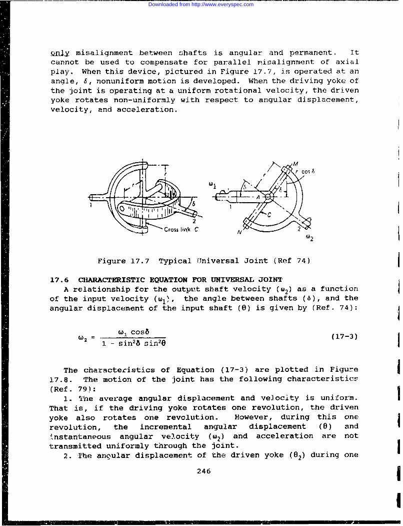
.Q11y misalignment between shafts is angular and permanent. Itcannot be used to compensate for parallel misa].ignment of axialplay. When this device, pictured in Figure 17.7, is operated at anangle, 6, nonuniform motion is developed. When the driving yoke ofthe joint is operating at a uniform rotational velocity, the drivenyoke rotates non-uniformly with respect to angular displacement,velocity, and acceleration.

2S"•_• Cross linik C w 2

Figure 17.7 Typical universal Joint (Ref 74)

17.6 CLARACTERISTIC EQUATION FOR UNIVERSAL JOINTA relationship for the output shaft velocity (W2) as a function

of the input velocity (wi), the angle between shafts (6), and theangular displacement of the input shaft (0) is given by (Ref. 74):

W2 Ca Cosa (17-3)1 - sin2 8 sin20

The characteristics of Equation (17-3) are plotted in Figure17.8. The motion of the joint has the following characteristics(Ref. 79):

1. The average angular displacement and velocity is uniform.That is, if the driving yoke rotates one revolution, the drivenyoke also rotates one revolution. However, during this onerevolution, the incremental angular displacement (0) andi.nstantaneous angular velocity (w2) and acceleration are nottransmitted uniformly through the joint.

2. The angular displacement of the driven yoke (02) during one 1246


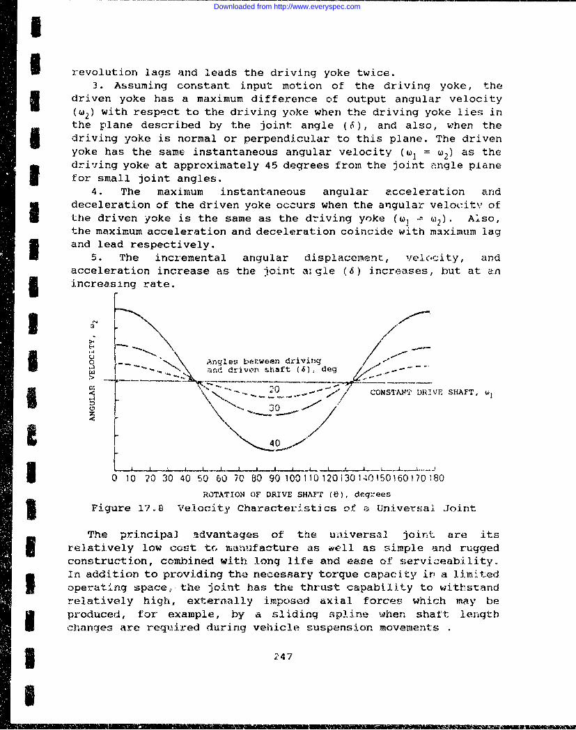
I i revolution lags and leads the driving yoke twice.3. Assuming constant input motion of the driving yoke, the

driven yoke has a maximum difference of output angular velocity

(w2) with respect to the driving yoke when the driving yoke lies inthe plane described by the joint angle (6), and also, when the3I driving yoke is normal or perpendicular to this plane. The drivenyoke has the same instantaneous angular velocity (wI = W2) as theI m driving yoke at approximately 45 degrees from the joint angle planefor small joint angles.

4. The maximum instantaneous angular acceleration anddeceleration of the driven yoke occurs when the angular velocity ofU the driven yoke is the same as the driving yoke (ý '= ()2). Also,the maximum acceleration and deceleration coincide with maximum lag

I and lead respectively.5. The incremental angular displacement, vel.ocity, and

acceleration increase as the joint aigle (6) increases, but at an3 increasing rate.

3 /

O ,N-N Angles btween driving

a nd driven~ Lhaft (6), deg

0-n CONSTANT DRIVE SHAFT, i

A ',

0 10 20 30 40 50 60 70 80 90 100110120i30140150160170180

ROTATION OF DRIVE SHAFT (6), degrees

Figure 17.8 Velocity Characteristics of a Universal Joint

The principal advantages of the universal joint are its3 relatively low cost tc, manufacture as well as simple and ruggedconstruction, combined with long life and ease of serviceability.In addition to providing the necessary torque capacity in a limitedoperating space, the joint has the thrust capability to withstandrelatively high, externally imposed axial forces which may beproduced, for example, by a sliding npline when shaft lengthchanges are required during vehicle suspension movements

3 I247

I


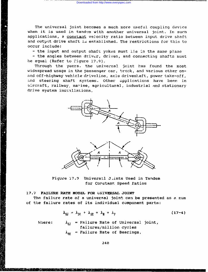
The universal joint becomes a much more useful coupling devicewhen it is used in tand,.m with another universal joint. In suchapplications, a constaat velocity ratio between input drive shaftand output. drive shaft iz established. The restrictions for this tooccur include:

- the input and output shaft yokes must lie in the same plane- the angles between driver, dr~i.ven, and connecting shafts must

be equal (Refer to rigure 17.9).Through the years. the universal joint has found the most

widespread usage in the passenger car, truck, and various other on-Sand off-highway vehicle driveline, axle drivesLaft, power take-off,.:,nd steering shaft systems. Other applications have been inaircraft, railway, marine, agricultural, industrial And stationarydrive system instollat.ions.

Figure 17.9 Universal Ji.nts Used in Tandemfor Corstant Speed Ratios

17.7 FAILUYRE RATE MODEL FOR UI1IVERSAL JOINTThe failure rate of a universal joint can be presented as a sum

of the failure rates of its individual component parts:

•UJ = XIB ÷ ASE + AH + )F (17-4)

Mhere: AUJ = Failure Rate of Universal joint,failures/million cycles

)BE = Failure Rate of Bearings,

248


failures/million cycles_sr. l Failure Rare of Seals,3 failures/million cyclesIl = Failure Rate of Structural Components,

failures/million cyclesF = Failure Rate of Coupling Fasteners,

failures/million cycles

3 The life expectancy of a joint is a function of the applicationrequirements such as torque, speed, and joint angle, as well asother factors. T7herefore, the basic load--speed--life-stressrelationships applicable to rolling element bearings are useful inlife computations for universal joints employing similar rollingelrnment'; These relationshi.ps have been established in the Bearingchapter of this Handbook. Although the contribution from termsother than in Equation (17-4) must be examined, in many cases ABEcan d; ive the relationship. For speed and load variation, basefailure rate is proportional to:

3 (LA ) Y,L!I

and:

NA

CN NA (17-6)

Where: LA = Actual radial loadLS = Specification radial load

Y = 3.33 for roller bearings3 Y = 3.00 for -iall bearingsNA = Actual speedN, = Specification speed

For more detailed component failure rate development, the userI is referred to the individual part chapters in this Handbook.

I3 249

I


THIS PACE INTENTIONALLY LEFTL BLANK

250


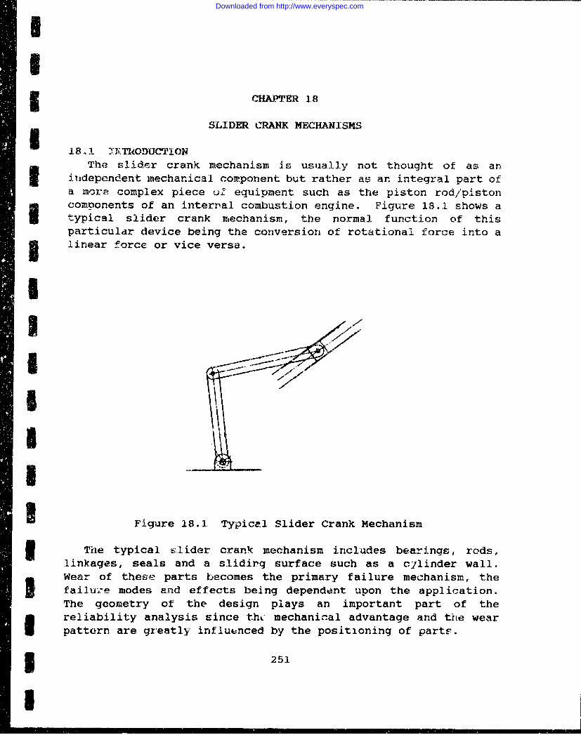
CHAPTER 1.8

SLIDER CRANK MECHANISMS

18 .1 XJ"NkODUCTIONThe slider crank mechanism is usually not thought of as an3 independent mechanical component but rather as an integral part of

a more complex piece uZ equipment such as the piston rod/pistong• components of an interral combustion engine. Figure 18.1 shows atypical slider crank mechanism, the normal function of thisparticular device being the conversion of rotational force into a3 I linear force or vice versa.

I

I| A

Figure 18.1 Typical Slider Crank Mechanism

3 The typical slider crank mechanism includes bearings, rods,linkages, seals and a slidirg surface such as a cjlinder wall.

Si Wear of these parts becomes the primary failure mechanism, thefailure modes and effects being dependent upon the application.The geometry of the design plays an important part of theI reliability analysis since tht: mechanical advantage and the wearpattern are greatlyj influenced by the positioning of parts.

3 251

-I


18.2 FAILURE MODES OF SLIDER CRANK MECHANISMSThe more predominant failure modes of a slider crank mechanism

can be readily identified with frictional actior on like ordissimilar materials. The component parts of a slider crankmechanism are subject to wear in varying degrees and the normalappro"Jh to reliability analysis is to escablish the expected lifeof the individual parts in the projected operating environment.

Bearing wear will usually be influenced by the lubrication filmthickness maintained, the side load on the bearing, thecontamination level, and corrosion. Chapter 7 presents an approachto evaluating bearing lite for theses ccnsiderations.

Slider crank wear will manifest itself in several ways to causethe degradation of the slider crank to the point of failure. Thisthreshold of failure must be defined in terms of jamming friction,side movement, limit of travel, alignment of parts, etc. Some ofthe failure modes to be considered are included in the followingtable.

TABLE 18-1

TYPICAL FAILURE MODES OF SLIDER CRANK MECAMNISMS

FAI UA= FAILURE CAUSELinkage does not move Bearing parts separatein intended direction causing jam

Restricted travel limited Excess load combined withof linkage loss of bearing material

Broken linkage Fatigue of linkage member

Linkage alignment out of Bearing deformedtolerance

The function of a mechanical seal is to provide a barrierbetween the moving or rotating surfaces and prevent the trapped

fluid from migrating into undesired areas. For example, in thecase of an engiae cylinder the rings on the piston prevent thecombustion gases from going into a lubricant and also prevent lossof energy due to combustion gas by-pass. The 0-ring and fiat sealsare designed to prevent the lubricant from contaminating other part

252


I areas and also, the loss of the lubriýcant. Seals and gaskets aredescribed in Chapter 3 and the models contained therein should be

* used for the analysis of seal and gasket reliability.Rods and linkages within the slider crank mechanism are subject

to fatigue and may crack although this failure mode is rare.

18.3 MODEL DLEVELOPMENTThe failure rate model for the sli". er crank mechanism can be3 eexpressed by the following equation:

Ssc = ABE +)R ASE + AI + A• (18-1)

Where: A• = Total failure rate for slider crank,failures/million operations

ABE = Failure rate for bearings, failures/millionoperations

SRD = Failure rate for rods/shafts, failures/millionoperations

ASE = Failure rate for seals/gaskets, failures/millionoperations

RI Failure rate for rings/dynamic seals,failures/million operations

A = Failure rate for sliding surface areas,failures/million operations

3 Reliability models can be developed for each specific part orparts and the combination of failure rates in accordance with the

I slider crank reliability model will provide the projected designlife.

U 18.3.1 BEARINGSOne of the predominant failure modes of a slider crank mechanism

is caused by a malfunctioning bearing surface. Both roller andU sliding bearings can be included in a slider crank design. Failurerate equations for roller/ball bearings are included in Chapter 7.

Typical sliding bearings are shown in Figure 18.2. The slidingbearing is usually comprised of three elements including the innersurface member, the outer surface member, and the lubricant filmseparating the inner and outer members. The sliding bearing ischaracterized as a shaft rotating within a sleeve. Slidingbearings can be classified by material, load direction, lubricationmethod, and configuration. Sliding bearings are well suited forlarge loads encountered in slider crank mechanisms. Although

3 253

I


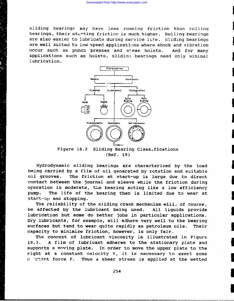
sliding bearings may have less running friction than rollingbearings, their strutting friction is much higher. Rolling bearingsare also easier to lubricate during service life. Sliding bearingsare well suited to low speed applicatir)ns where shock and vibrationoccur such as punch presses and steam hoists. And for manyapplications such as hoists, slidinc,, bearings need only minimallubrication.

LZFE]

Matallic Nonmgtallic

i I]I

(Loaing) ( Lu~eation) (Configuration)

so_ i t

Hydrodynamic Hydrostatic Slf.lubrication

Figure 18.2 Sliding Bearing Classifications(Ref. 19)

Hydrodynamic sliding bearings are characterized by the loadbeing carried by a film of oil generated by rotation and suitableoil grooves. The friction at start-up is large due to directcontact between the journal and sleeve while the friction duringoperation is moderate, the bearing acting like a low efficiencypump. The life of the bearing then is limited due to wear atstart-'up and stopping.

The reliability of the sliding crank mechanism will, of course,be affected by the lubricant being used. All liquids providelubrication but some do better jobs in particular applications.Dry lubricants, for example, will adhere very well to the bearingsurfaces but tend to wear quite rapidly as petroleum oils. Theircapacity to minimize friction, however, is only fair.

The concept of lubricant viscosity is illustrated in Figure18.3. A film of lubricant adheres to the stationary plate andsupports a moving plate. In order to move the upper plate to theright at a constant velocity V, it is necessary to exert somec otnnt force F. Thus a shear stress is applied at the wetted

254


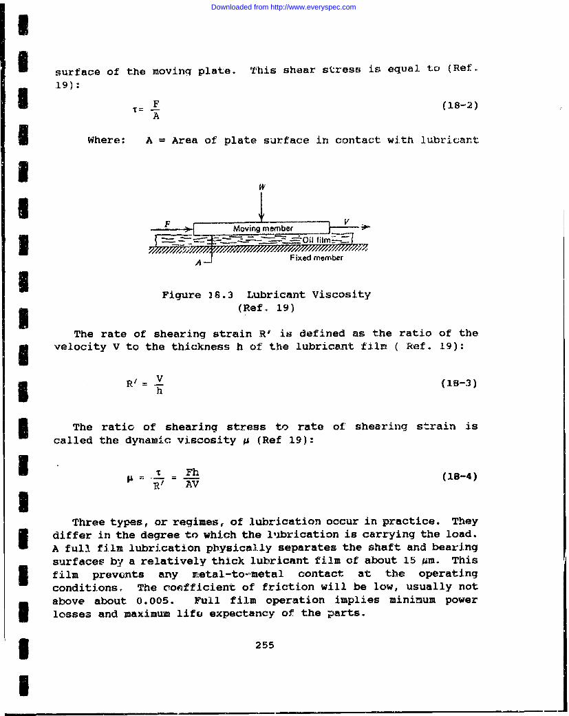
,I

I surface of the movinq plate. This shear stress is equal to (Ref.

19): F (18-2)

A

I Where: A = Area of plate surface in contact with lubricant

3Wa~wF.. Moving memer--

A- Fixed member

Figure 18.3 Lubricant Viscosity3 (Ref., 19)

The rate of shearing strain R' is defined as the ratio of theI velocity V to the thickness h of the lubricant filn( Ref. 19):

1R/ = (10-3)h

5 The ratio of shearing stress to rate of shearing strain iscalled the dynamic viscosity p (Ref 19):

I _ Fh (18-4)-Rt AV (84

Three types, or regimes, of lubrication occur in practice. TheyI differ in the degree to which the lubrication is carrying the load.

A full film lubrication physically separates the shaft and bearingsurfaces by a relatively thick lubricant film of about 15 gm. Thisfilm prevonts any metal-to--metal contact at the operatingconditions. The coefficient of friction will be low, usually notabove about 0.005. Full film operation implies minimum powerlosses and maximum lifo expectancy of the parts.

5 255

I


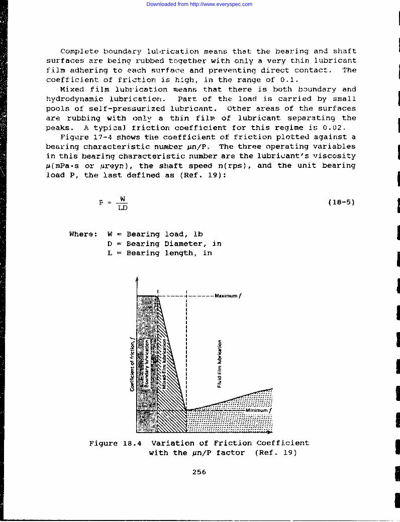
Complete b.,oundary lubricati-on means that the bearing and shaftsurf aces are being ruibbed together with only a very t~hin lubricantfilm adhering to ech surfnooce and preventing direct Contact'. Thecoefficient of fric~tion is high, in the range of 0 .1.

MixedJ film lubrication means that there is both boundary andhydrodynamic lubrication. Part of the load i~s carried by smallpools of self -pre. sur:Lzed lubricant. Other areas of the surfacesare rubbing with oni",u a thin filp. of lubricant separating the

peaks. A typicaJ triction coefficient for this regime is 0.02.Figure 17-4 shows the coefficient of friction plotted against a

bearing characteristic number sin/P, The three operating variables

in this bearing characteristic number are the lubricant's viscosityp(xnPa-s or /hreyn), the shaft speed n(rps), and the unit bearingload P, the last defined as (Ref. 19):I

P = -W(18-5)1

Where: W = Bearing load, lbjD =Bearing Diameter, inL Bearing length, in

-4

I eI

with the Mn/P factor (Ref. 19)

2561


I

I This bearing characteristic number provides a method ofdetermining any potential problem with lubricant film. Any low

I viscosity, low shaft speed, or high unit bearing load implies a lowvalue for gn/P. Conversely, the higher gn/P, the easier it is toestablish a full-load-supporting film.

For the largest values of pn/P, there is full-fluid-film, orhydrodynamic, lubrication. In this regime of operation thecoefficient of friction attains a minimum of about 0.001. A3 greater gn/P value will assure an adequately thick film and amargin of safety with a somewhat greater power loss.

The lowest values of Mn/P correspond to the regime of completeboundary lubrication. The friction coefficient remains constantthroughout this regime; its actual value depends on the characterof the surfaces and the lubricant.

The midregime is that of mixed-film lubrication. In this regimea decrease in pn/P is accompanied by a sharp increase in friction

I coefficient.Most of the bearings utilized in mechanical devices are

considered light service and operate in the mixed-film or boundaryI lubrication regimes. Typical office equipment and appliances withlatching mechanisms contain bearings with little or even nolubrication and without the proper operating conditions to developa full-lubricant film. Yet they survive and they provide a low-cost solution to the problem of supporting and controlling machinemembers in relative motion.

Manufacturers of bearings for light service usually base bearingselection on the PV factor, the product of unit bearing load P andrubbing velocity V. This factor indicates what bearing temperaturewill be reached and what rate of wear can be expected. Temperaturerise and wear rate are maintained within reasonable limits by

I controlling the PV factor.The unit bearing load P, already defined by Equation (18-5) is

the ratio of the bearing's load to its projected area. The zubbingI velocity V must be calculated differently for oscillating shaft

motion than for continuous rotation. For continuous rotation therubbing speed is (Ref. 19),I

V ý 5nDn (18-6)IWhere: V = rubbing veloci ty, fpm

D = bearing diameter, inn = shaft speed; rps

3 257

I


However, if the shaft is oscillating relative to the bearing,the design value for V is based on the average rubbing speed (Ref19).

V 7D~ f (18-7) D72

Where: 0 = Total angle traveled per cycle, degf = Frequency of oscillation, cps

The use of sleeve or journal bearings in severe service requiresa full bearing or a thick lubrication film to support the load.While an external pump may be used to supply a lubricant underpressure to the bearing's feed hole, within the bearing itself itis the shaft that acts as a pump and pumps the oil adhering to itinto the wedge-shaped oil film that supports the load. With theshaft stationary, the shaft simply rests on the bottom of thebearing. But at start-up the shaft begins to roll up the bearingwall. As it climbs, it also begins to pump oil between itself andthe bearing. As this oil is pumped, the shaft lifts off thebearing surface and moves in the direction of rotation. Atoperating speed, the shaft has developed a wedge-shaped filmbetween itself and the bearing that supports the shaft and itsload. The radial displacement of the shaft's center from thebearing's center is the eccentricity, e. The pressure distributionin the oil film achieved depends on factors such as shaft speed,load, lubricant viscosity, bearing clearance, and length-to-diameter ratio.

18.3.2 Re.!ShaftaThe reliability of the rod or shaft is generally very high when

compared to tho components in the sliding-action system. Generally,the life expectancy will be at least three times that of thebearing. The possibility that the rod or shaft will fracture canbest be determined using finite element techniques. The effects ofthe rod or shaft breakage on adjacent components is of greaterimportance than the reliability of the rod or shaft itself. FromChapter 10 the following equation for rod or shaft failure rate isderived:I

A: S = S,B * CP • CF CSE COO (18-8)

Where: ASA,B Rod or shaft base failure rate

258


CASF ' Surface finish factorCDF ' Material temperature fectnrCSE Material endurance factorCON =Contamination factor

Procedures for determining the base failure rate and themultiplying factors can be found in Chapter 10.

I 18.3.3 Seals/Gaskets

The failure rate of a seal or gasket is determined by ability ofthe seal to restrict the flow of fluid frow one region to anotherfor the intended life is prescribed operating environment. FromSection 3.2 of Chapter 3 the followinq equation is d3rLved for

* determining the failure rate.

XSE = I SE,B CP CQ 9 CDL o CH e Cf • CU • Ct . CY (18-9)

Where: ISE, = Base failure rate of seal,0.85 failures/million operations

C = Multiplying factor which considers theeffect of fluid pressure on ASEB

CQ = Multiplying factor which considers theI effect of allowable leakage on ASE,

DL= Multiplying factor which considers theeffect of seal size on ASE,B

C = Multiplying factor which considers theeffect of seal hardness and tightnesson ASE,BSf = Multiplying factcr which considers theeffect of seat smoothness on ASE,B

SCv Multiplying factor which considers theeffect of fluid viscosity on ASEB

Ct= Multiplying factor which considers theeffect of temperature on ASE,B

C, Multiplying factor which considers theeffect of contaminants on ASEB

The procedures contained in Chapter 3 can be used to determineI the base failure rate and multiplying factors.

18.2.4 D•M1 ic SealsThe sealing surface of rings and other dynamic seals are

perpendicular to the shaft with contact between primary and

3 259

I


rings to achieve a dynamic seal at various speeds, pressuý -- andtemperatures. From section 3.3 of Chapter 3 the following equacionis derived for determining the failure rate of a dynamic seal.

)SE = ISE,B * CQ * CH • Cf • Cy * Ct • CN . CPV (18-1 )

Where: C• = Multiplying factor which considerE theeffect of the seal PV value on ISF,B

The procedures contained in Chapter 3 can be used to determinethe base failure rate and multiplying section for rings.

18.3.5 = Suf--. AreaThe wear life of the sliding surface area depends on the

correlation of wear of the two surfaces involved with the materialstrength and the stress imposed on the sliding action mechanism.From a time vtandpoint, wear of the two surfaces will occur in twophases. The first or constant wear phase is characterized by theshearing of asperities due to sliding action. During this periodthe wear rate is practically linear as a function of the numnber ofmechanical cycles and the wear depth at the end of the constantwear phase is one half the original surface finish. During thesecond or severe wear phase, wear debris becomes trapped betweenthe two sliding surfaces and gouging of the surfaces takes place.The wear rate begins to increase very rapidly and failure of thesliding action mechanism is imminent. From Chapter 9, Section9.3.1:

AAC = XAC.B CCp D CT (18-11)

Where: AC = Failure rate of actuator, failures/millioncycles

CCP =Contaminant particle coefficientCT= Temperature factor

Section 9.3.1 of Chapter 9 describes a procedure to determinethe number of cycles in Phase 1 wear and the number of cycles inPhase 2 wear at which point the slider crank mechanism isdetermined to have tailed.

260


CHAPTER 19

REFE ES,

1. Aoadzheva, R.N. et al., "Effects of Brake Fluid Components orRubber," Khimiya i Tekhnologiya Topliv i Masel, No. 8, pp. 18-u 19 (Aug 1982).

2. AILker, I.G et al., "rrocedure for Calculating theWorking Characteristics o' Clutcher for Motor Cars,Tractors, and Other Macnines During the Design Stacle,"Vestnik Mashinostroonlya, Vol. 63, Yo. 3 (1982).

3. Anderson, A.E., "Wear of Brake !Vaterials," in: Wear ControlHandbook, M.B. Peterson and W.O. Winer, Eds., pp. 843-857, An.3 Soc. Mech. Eng., New York (1900).,

4. Armstrong, E.L., V.R. Murphy and P.S. Wooding,"Evaluation of Water Accelerat3d Bearing Fatigue in Oil-Lubricated Ball Bearings," Lubricatin Enginoerin, Vol.34, No. i, pp. 15-21 (1 Nov 1977).

5. Bauer, P., M. Glickmon, and F. Iwatsuki, "Analyticalh for the Design of Seals for JleinRkocke

2.rQRulsion Systems," Volume 1, ITT Research Institute,Technical Report AFRPL-TR-65-61 (May 1965).

3 6. Bayer R.G., A.T. Shalhey and A.R. Watson, "Designing for ZeroWear," Mj~ neD_•1gZj (9 January 1970).

I 7. Bishop, F.E. and William M. Needleman, "The Effects of FluidContamination on Component Wear," Pall Corporation.

I S. Block, H. and D. Johnson, "Downtiue Prompts Upgrading ofCentrifugal Pumps," 9j i1 Engineering Njagzine, pp. 35-733 (25 Nov 1985).

9. Boone, Tony D., "Reliability Prediction Analysis forSMechanical Brake Systems," NAVAIR-SYSCOM Report (Aug 1981),

10. "Boston Gear Catalog" Catalog 100, INCOM Internatioiial Inc.,I Quincy, Massachusetts 021.71.

3 261

I


ii. Canterbury, Jack, and James D. Lowther, "dApplication ofDimensional Analysis to the Prediction of MechanicalReliability," Haval Weapons Support Activity, Washington NavyYard, Wash., D.C., Report ADAD35295 (September 1976).

12. Carson, Harold, 5__e oi&jtya"., Marcel Dekker, Inc., New York. (1983).

13. Cormier, K.R., "Helicopter Drive System R&M Design Guide,"Division of United Technologies Corp., Stanford, CT 06602,Report ADAD69835 (April 1979).

14. "Engineering Guide to Spring Design" Associated Spring, BarnesGroup INc., Form No. 515 (1981).

15. "Fabrication and Testing of Lightweight Hydraulic SystemSimulator Hardware - Phase II," Report NADC-79024-60, preparedby Rockwell International, Columbus, Ohio, for Naval AirSystems Command, Washington, D.C.

16. Ferodo Limited, Friction Materials for Engineers, Stockport,England (1969).

17. Field, G.J., "Seals That Survive Heat," XjfljgDe (1 May1975).

18. Hauser, D.L. el: al., "Hardness Tester for Polyur," liALAbhbif, Vol. 11, No. 6, p. 57 (1987).

19. Hindhede et al., Machine Design Fundamentals (1983).

20. Ho, T.L., F.E. Kennedy and M.B. Peterson, "Evaluation ofMaterials and Design Modifications for Aircraft Brakes," NASARepQr. CR134896 (Jan 1975).

21. Houston, John, "Getting to Grips with Clutches and Brakes,"in: Engineering Materials and Design, Vol. 26, No. 4 (April19821).

22. Howell, Glen W. and Terry M. Weathers, Aerospace FluidCcmponent t igDl J nm- Q, Volumes I and I!, TRW SystemsGroup, Redondo Beach, CA prepared for Air Force RocketPropulsion Laboratory, Edwards, CA, Report AD 874 542 and I

262

I


I Report AD 874 543 (February 1970).

23. Hubert, Christopher J., John W. Beck and John H. Johnson, "AI Model and the Methodology for Determining Wear ParticleGeneration Rate and Filte: Efficiency in a Diesel Engine UsingFerrography," Society of Automotive Engineers Paper No. 821195(1982).

I 24. Hudgens, R.D. and L.B. Feldhaus, "Diesel Engine Lube FilterLife Related to Oil Chemistry," Society of Automotive1Er'gineers Paper No. 780974 (1978).

25. Juhnson, R.L. and K. Schoenherr, "Seal Wear," in: iegarrC ontrol HAnbQp, M.R. Peterson and W.O. Winer, Eds., Sect. 5,pp 727-754, American Society of Mechanical Engineers, NewYork, (1980).

1 26. Krutzsch, W.C., Pum HadbQoK, McGraw-Hill Book Company, newYork (1968).

27. May, K.D., "Advanced Valve Technology," National Aeronauticsand Space Administration, NASA Report SP-5019 (February 1965).

28. MIL-HDBK-21'vD, "Reliability Prediction of ElectronicEquip1tent" (Jaruary 1982).

29. Minegisbi, H. et al., "Prediction of Brake Pad Wear/Life byMeans of Brake Severity Factor as Measured on a Data LoggingSystem," SAE Paper 840358 (1984).

30. Mordkowitz, A., "Predicting Service Life for Zero Wear,"Kjn.LQign (10 January 1974).

I 31. Nagel, W.B., "Designing wi-h Rubber," Machine Design (June 23,July 7, July 21, Aug 1, 1977).

32. Neale, M.J., Tribology Handbook, Butterworths, London.

33 Needleman, William K., "Filtration for Wear Control," in-r a M.B. Peterson and W.O. Winer, Eds.,

Sect. 4, pp 507-582, Americna Society of Mechanical Engineers,iNew York, (1980).

3 263

I


34. Newcomb, T.P., "Thermal Aspects of Vehicle Braking,"Automobile Engineering (Aug 1960).

35. "Optimum Design of Helical Springs," Machine Design, (6November 1980).

36. Orthwein, William C., Clutches and Brakes: Design andSelection, Marcel Dekker, Inc., New York (1986).

37. Rhee, S.K. and P.A. Thesier, "Effects of Surface Roughness ofBrake Drums on Coefficient of Friction and Lining Wear," SAEPaper 720449 (1972).

38. Roack and Young, £ l __f_ an_2_rp- McGraw-HillBook Company, New York (1975).

39. Shigley, Joseph E., JcI __gnej•rtg1gaign, McGraw-Hill, Inc., New York, NY (1977).

40. Spokas, R.B., "Clutch Friction Material EvaluationProcedures," SAE Paper 841066 (1984).

41. "Standard Product Catalog," Catalog SPC 82, The FalkCorporation, Milwaukee, Wisconsin.

42. Weintraub, M.H. et al., "Wear of Resin Asbestos FrictionMaterials," in: Advances in Polymer Friction and Wear, pp.623-647.

43. Wilhelm, James P. and Andrew V. Loouis, "Brake FrictionMaterials: A Market Survey," NASA Report (Aug 1975),

44. Sibley, L.B., "Rolling Bearings," in: Wear Control Handbook,M.B, Peterson and W.O. Winer, Eds., Sect. 5, pp 699-726,American Society of Mechanical Engineers, New York (1980).

45. Barron, Randall V., Reyiaion ogfWear Model for Stock

AgQrfl -i1f ng ModelJ•f fQr Mechanical Wear (July 1987).

46. Fox, R.W., and A.T. McDonald, Introduction to Fluid Mechanics,John Wiley and Sons, New York (1978).

264


I

IJ 47. Machine Design, 1985 Fluid Power Reference Issue, Penton/IPC,Inc., (Sept. 19, 1985).

I . Bayer, R.G., A.T. Shalkey, and A.R. Watson, "Designing forZero Wear," H eDs , Vol. 41, pp. 142-151 (1969).

I 49. Kragelsky, I.V. arid V.V. Alisin, Frigtion. Wear. andI L~k io~i~n, Vol. 2, pg. 30, Pergamon Press, London (1981).

50. Kuhlmann-Wildorf, D., "Parametric Theory of Adhesive Wear inUni-Directional Sliding," Wear Qf Itria, pp. 402-413,American Society of Mechanical Eigineers, New York (1983).

51. Bentley, R.M. and D.J. Duquette, "Environmental Considerationsin Wear Processes," EUndadmentIs of Friction and Wear 3fMaterial, pp. 291-329, American Society For Metals, Metals5 Park, Ohio (1981).

52. Sarkar, A.D., Wear of Metala, pp. 62-68, Pergamon Press,3 London (1976).

53. Lundberg, G. and A. Palmgren, "Dynamic Capacity of RollingBearings," Acta Poleftechnica, No. 7 (1974).

54. Rumbarger, John H., "A Fatigue Life and Reliability Model forGears," American Gear Manufacturers Association Report 229.16(January 1972).

I 55. AGMA Standard for Surface Durability Formulas for Spiral BevelGear Teeth, American Gear Manufacturers Association Report216.01 (January 1964).

56. AGMA Standard Nomenclature of Gear Tooth Failure Modes,American Gear Manufacturers Association Report 110.04 (August1980).

I 57. Haviland, G.S., "Designing with Threeded Fasteners",MECHANICAL ENGINEERING, Vol 105, No. 10, Oct 83.

3 58. Deutschman, A.D., et al, Machine Design; Theory and Practice,MacMillan Publishing Co, NY, 1975

I3 265

I


59. Parmley, R.O., Mechanical Components Handbook, McGraw-Hil.,Book Co., NY, 1985.

60. Handbook H28, Nat'l Bureau of Stds, Govt Printing Office,Washington, DC, 1957.

61. Hindhede, U., et al, Machine Design Fundamentals, John Wiley& Sons, NY, 1983.

62. Shigley, J.E., Mischke, C.R., Mechanical Engineering Design,McGraw-Hill Book Co., NV, 1989.

63. Bickford, J.H., An Introduction to the Design and Behavior ofBolted Joints, Marcel Dekker, Inc., NY, 1990.

64. Handbook of Corrosion Data, ASM International, Metals Park,OH, 1990

65. Baumeister, T, et al, Mark's Standard Handbook for ehanicalginiratur

66. Thomas Couplings Applications Manual

67. Bolam, J.R., "Coupling Alignment: The Reverse IndicatorMethod Simplified", P/PM Technology, July/Aug 90

68. Deutschman, A.D., et al, Machine Design; Theory & Practice,Aacmillan Publishing Co,Inc. NY,NY.

69. Parmley, R.O., IN2chanicai Components Handbook, McGraw-HillBook Co. NY,NY, 1985.

70. Dvorak, P., "Sorting Out Flexible Couplings", Machine Design,11 Aug 88

71. Robertson, R., and Smith, B., "Why Flexible Couplings Fail",PlantmaiF n ring and Maintenance, Jun 89

72. Universal Joint & Driveshaft Design hanual, Series No. 7,Society of Automotive Engineers, Inc, Warrendale, Pa.

73. Anderson, Edwin P., Electric Motors Handbook, Bobbs-MerrillCo., Inc., NY, NY 1983

266


SI INITIAL DISTRI•,•LXON

I Copies

2 ONT3 ONT 226 CDR D. Bennett

I6 NAVAIR4 AIR-5115 R. Trakas1 AIR-411 D. Stacey1 AIR-411 J. McKendrew

5 Robins AFB5 WR-ALC/LVRS C. Perrazola

5 Picatinny Arsenal5 SMCAR-QAH-P S. HarkowitL

2 NAVSEA1 SEA-04 C. Geiger1 SEA-5121 M. Buckberg

2 NAVSUP1 SUP-642C J. mays1 SUP-4233 R. Whitfield

2 Belvoir RD&E Center1 SRRBE-TQR C, NeeseI STRBE-TQR L. Jackson

5 2 OP-4031 OP-403R CDR R. Thomas1 OP-403R K. Stabenau

1 Wright-Patterson AFB1 AFHRL/LRL W. Cambell

1 Rome Air Development Center1 RL/ERSR M. McCallum

26 CARDERrCKDIV, NSWC1 Code 03 CAPT D. Kruse1 Code 0i R. Metry1 Code 01. H. Chaplin5 Code 0116 R. Brengs1 Code 1.2 G. KerrI Cde 1.25 R. Schaffran1 Code 129 R. Plc.10 Code 1290 J. Chesley5 Code 2J432 Reports Control

I!


Handbook of Reliability Prediction Procedures for Mechanical ...

Documents