
Welcome message from author
This document is posted to help you gain knowledge. Please leave a comment to let me know what you think about it! Share it to your friends and learn new things together.
Transcript

/

Handbook of Geotechnical Investigation and Design Tables

B A L K E M A - Proceedings and M onographs in Engineering, Water and Earth Sciences
Handbook of Geotechnical Investigation and Design Tables
Burt G. LookConsulting Geotechnical Engineer
Taylor & FrancisTaylor &. Francis GroupLONDON / LEIDEN / NEW YORK / PHILADELPHIA / SINGAPORE
30 f i09
Taylor & Francis is an imprint o f the Taylor <&' Francis G roup , an informa business
© 2 0 0 7 Taylor & Francis Group, London, UK
Typeset by Charon Tec Ltd (A Macmillan Company), Chennai, India Printed and hound in Great Britain by TJ International Ltd, Padstow, Cornwall
All rights reserved. No part of this publication or the information contained herein may be reproduced, stored in a retrieval system, or transmitted in any form or by any means, electronic, mechanical, by photocopying, recording or otherwise, without written prior permission from the publishers.
Although all care is taken to ensure integrity and the quality of this publication and the information herein, no responsibility is assumed by the publishers nor the author for any damage to the property or persons as a result of operation or use of this publication and/or the information contained herein.
Published by: Taylor & Francis/BalkemaP.O. Box 4 4 7 , 2 3 0 0 AK Leiden, The Netherlands e-mail: Pub.NL@tandf .co.ukwww.balkema.nl ,www.taylorandfrancis .co.uk,www.crcpress.com
Library o f Congress Cataloging-in-Publication Data Look, Burt.
Handbook of geotechnical investigation and design tables / Burt G. Look, p. cm.
ISBN 9 7 8 - 0 - 4 1 5 - 4 3 0 3 8 -8 (hardcover: alk. paper) 1. Engineering geology— Handbooks, manuals, etc. 2. Earthwork. I. Title.
TA70.5.L66 2 0 0 76 2 4 . 1 ' 5 1 — dc22 2 0 0 6 1 0 2 4 7 4
ISBN 13: 9 7 8 - 0 - 4 1 5 - 4 3 0 3 8 -8 (hardback)ISBN 13: 9 7 8 - 0 - 2 0 3 - 9 4 6 6 0 - 2 (e-book)
Table of Contents
Preface
I Site investigation
1.1 G eotechnical involvement 1
1.2 G eotechnical requirements for the different project phases 2
1.3 Relevance o f scale 3
1.4 Planning o f site investigation 3
1.5 Planning o f groundwater investigation 4
1.6 Level o f investigation 4
1.7 Planning prior to ground truthing 4
1.8 Extent o f investigation 6
1.9 Volume sam pled 9
1.10 Relative risk ranking o f developm ents 9
1.11 Sample amount 9
1.12 Sample disturbance 11
1.13 Sample size 1 2
1.14 Quality o f site investigation 12
1.15 Costing o f investigation 13
1.16 Site investigation costs 14
1.17 The business o f site investigation 15
Soil classification 17
2.1 Soil borehole record 17
2.2 Borehole record in the field 18
2.3 Drilling information 19
2.4 Water level 19
2.5 Soil type 19
2.6 Sedimentation test 20
2.7 Unified soil classification 20
2.8 Particle description 22
vi Table of Contents
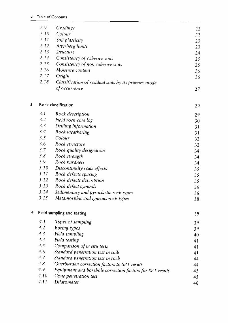
2 .9 C /’ railings 222.10 Colour 222.11 Soil plasticity 232.12 At ter berg limits 232.13 Structure 242.14 Consistency o f cohesive soils 252.15 Consistency o f non cohesive soils 252 .1 6 M oisture content 262 . 1 7 Origin 262.18 Classification o f residual soils by its primary m ode
o f occurrence 27
3 Rock classification 29
3.1 Roc£ description 293.2 Field rock core log 303.3 Drilling inform ation 313.4 R ock weathering 313 .5 C olour 323 .6 structure 323 . 7 R ock quality designation 343.# strength 343 .9 hardness 343 . 2 0 Discontinuity scale effects 353 . /I R ock defects spacing 353.12 Rock defects description 353.13 Rock defect sym bols 363.14 Sedimentary and pyroclastic rock types 363.15 M etam orphic and igneous rock types 38
4 Field sampling and testing 39
4.1 Types o f sampling 394.2 Boring types 394.3 Field sam pling 404.4 Field testing 414.5 C om parison o f in situ tests 414 .6 Standard penetration test in soils 414.7 Standard penetration test in rock 444.8 O verburden correction factors to SPT result 444 .9 Equipm ent and borehole correction factors for SPT result 454 . 10 Cone penetration test 454.11 D ilatom eter 46
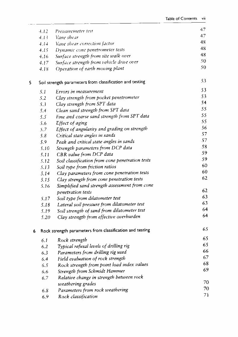
Table of Contents vii
4.12 Pressuremeter test 47
4 .1 i Vane shear 47
4.14 Vane shear correction factor 48
4.15 Dynamic cone penetrom eter tests 48
4 .16 Surface strength from site walk over 48
4.17 Surface strength from vehicle drive over 50
4.18 O peration o f earth moving plant 50
5 Soil strength parameters from classification and testing
5.1 Errors in measurement 53
5.2 Clay strength from pocket penetrom eter 53
5.3 Clay strength from SPT data 54
5.4 Clean sand strength from SPT data 55
5.5 Fine and coarse sand strength from SPT data 55
5.6 Effect o f aging 55
5.7 Effect o f angularity and grading on strength 56
5.8 Critical state angles in sands 57
5.9 Peak and critical state angles in sands 57
5.10 Strength parameters from DCP data 58
5.11 CBR value from DCP data 59
5.12 Soil classification from cone penetration tests 59
5.13 Soil type from friction ratios 60
5.14 Clay param eters from cone penetration tests 60
5.15 Clay strength from cone penetration tests 62
5.16 Sim plified sand strength assessment from conepenetration tests 62
5.17 Soil type from dilatom eter test 63
5.18 Lateral soil pressure from dilatom eter test 63
5.19 Soil strength o f sand from dilatom eter test 64
5.20 Clay strength from effective overburden 64
6 Rock strength parameters from classification and testing 65
6.1 R ock strength 65
6.2 Typical refusal levels o f drilling rig 65
6.3 Parameters from drilling rig used 66
6.4 Field evaluation o f rock strength 67
6.5 R ock strength from point load index values 68
6.6 Strength from Schmidt Hammer 69
6.7 Relative change in strength between rockw eathering grades 70
6.8 Param eters from rock weathering 70
6.9 R ock classification 71
viii Table of Contents
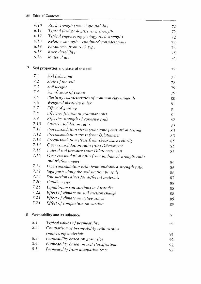
6.10 R ock strength from slope stability 726.11 Typical field geologists rock strength 726.12 Typical engineering geology rock strengths 726.1 3 Relative strength - com bin ed considerations 736 .14 Parameters from rock type 746.1 S R ock durability 756.16 Material use 76
Soil properties and state of the soil 77
7.1 Soil behaviour 777.2 State o f the soil 787.3 Soil weight 797.4 Significance o f colour 797.S Plasticity characteristics o f com m on clay minerals 807.6 Weighted plasticity index 817 7/. / Effect o f grading 817.8 Effective friction o f granular soils 817.9 Effective strength o f cohesive soils 827 AO O verconsolidation ratio 837.11 Preconsolidation stress from cone penetration testing 837.12 Preconsolidation stress from Dilatometer 837 .1] Preconsolidation stress from shear wave velocity 857.14 O ver consolidation ratio from Dilatometer 857.1 S Lateral soil pressure from D ilatom eter test 857.16 O ver consolidation ratio from undrained strength ratio
and friction angles 867.17 O verconsolidation ratio from undrained strength ratio 867.18 Sign posts along the soil suction pE scale 867.19 Soil suction values fo r different materials 877.20 Capillary rise 887.21 Equilibrium so il suctions in Australia 887.22 Effect o f climate on soil suction change 887.23 Effect o f clim ate on active zones 897.24 Effect o f com paction on suction 89
Permeability and its influence 91
8.1 Typical values o f perm eability 918.2 Com parison o f perm eability with various
engineering materials 918.3 Permeability based on grain size 928.4 Permeability based on soil classification 928.S Permeability from dissipation tests 93
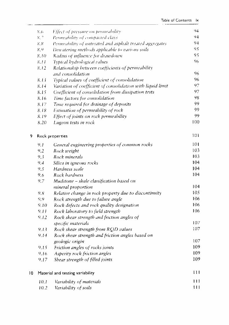
Table of Contents ix
■S’. 6 1 ffect o f pressure on perm eability 94
8 .7 Permeability o f com pacted clays 94
s. 8 Permeability o f untreated and asphalt treated aggregates 94(S’. 9 Dewatering m ethods applicable to various soils 95
8.10 Radius o f influence for draw dow n 95
8. 11 Typical hydrological values 96
8. 12 Relationship betw een coefficients o f perm eabilityand consolidation 96
8.11 Typical values o f coefficient o f consolidation 96
8.14 Variation o f coefficient o f consolidation with liquid limit 97
8.15 C oefficient o f consolidation from dissipation tests 97
8 .16 Time factors fo r consolidation 98
8.17 Time required fo r drainage o f deposits 99
8.18 Estimation o f permeability o f rock 99
8.19 Effect o f joints on rock perm eability 99
8.20 Luge on tests in rock 100
Rock properties 101
9./ General engineering properties o f com m on rocks 101
9.2 Rock weight 1039 J Rock minerals 1039.4 Silica in igneous rocks 104
9.5 Elardness scale 104
9.6 Rock hardness 104
9.7 M udstone - shale classification based onmineral proportion 104
9.(S} Relative change in rock property due to discontinuity 1059.9 R ock strength due to failure angle 1069. / 0 Rock defects and rock quality designation 1069./ / Rock laboratory to field strength 106
9.12 Rock shear strength and friction angles o fspecific m aterials 107
9 .M R ock shear strength from RQ D values 107
9./4 R ock shear strength and friction angles based ongeologic origin 107
9 .75 Eriction angles o f rocks joints 109
9. / 6 Asperity rock friction angles 109
9 .17 Shear strength o f filled joints 109
Material and testing variability 1 1 1
10.1 Variability o f materials 11 1
10.2 Variability o f soils 1 11
x Table of Contents
10.3 Variability o f in-situ tests10.4 Soil variability from laboratory testing10.5 Guidelines fo r inherent soil variability10.6 Com paction testing10.7 Guidelines fo r com paction control testing10.8 Subgrade and road material variability10.9 Distribution functions10.10 Effect o f distribution functions on rock strength10.11 Variability in design and construction process10.12 Prediction variability for experts com pared with
industry practice10.13 Tolerable risk for new and existing slopes10.14 Probability o f failures o f rock slopes10.15 Acceptable probability o f slope failures10.16 Probabilities o f failure based on
lognorm al distribution10.17 Project reliability10.18 R oad reliability values
I I Deformation parameters
11.1 Modulus definitions11.2 Small strain shear modulus11.3 Com parison o f small to large strain modulus11.4 Strain levels fo r various applications11.5 Modulus applications11.6 Typical values fo r elastic parameters11.7 Elastic param eters o f various soils11.8 Typical values for coefficient o f
volume compressibility11.9 Coefficient o f volume compressibility derived
from SPT11.10 D eform ation parameters from CPT results11.11 Drained soil modulus from cone penetration tests11.12 Soil modulus in clays from SPT values11.13 Drained modulus o f clays based on
strength and plasticity11.14 Undrained modulus o f clays for varying over
consolidation ratios11.15 Soil modulus from SPT values and plasticity index11.16 Short and long term modulus11.17 Poisson ratio in soils11.18 Typical rock deform ation parameters
112113114 114 114 1 14 1 15 116 117
117118118119
119120 120
121121123123123125126 126
128
128129129130
130
130131 131131132
Table of Contents xi
11.19 Rock deform ation parameters 132
11.20 Rock mass modulus derived from the intact rock modulus 133
11.21 Modulus ratio based on open and closed joints 133
11.22 Rock modulus from rock mass ratings 133
11.23 Poisson ratio in rock 134
11.24 Significance o f modulus 135
2 Earthworks 137
12.1 Earthw orks issues 137
12.2 Excavatability 137
12.3 Excavation requirements 137
12.4 Excavation characteristics 139
12.5 Excavatability assessment 139
12.6 Diggability index 139
12.7 Diggability classification 140
12.8 Excavations in rock 140
12.9 Rippability rating chart 141
12.10 Bulking factors 142
12.11 Practical maximum layer thickness 143
12.12 Rolling resistance o f w heeled plant 143
12.13 C om paction requirements for various applications 144
12.14 Required com paction 145
12.15 Com parison o f relative com paction andrelative density 146
12.16 Field characteristics o f materials used in earthw orks 146
12.17 Typical com paction characteristics o f materials usedin earthw orks 146
12.IS Suitability o f com paction plant 146
12.19 Typical lift thickness 149
12.20 Maximum size o f equipm ent based on permissiblevibration level 150
12.21 Com paction required fo r different height o f fill 150
12.22 Typical com paction test results 150
12.23 Field com paction testing 150
12.24 Standard versus m odified com paction 152
12.25 Flffect o f excess stones 152
13 Subgrades and pavements 153
13.1 Types o f sub grades 153
13.2 Subgrade strength classification 154
13.3 Damage from volumetrically active clays 154
xii Table of Contents
13.4 Subgrade volume change classification 15413.5 Minimising subgrade volume change 15513.6 Subgrade moisture content 15613.7 Subgrade strength correction factors to soaked CBR 15713.8 Approxim ate CBR o f clay subgrade 15713.9 Typical values o f subgrade CBR 15713.10 Properties o f mechanically stable gradings 15813.11 Soil stabilisation with additives 15913.12 Soil stabilisation with cement 15913.13 Effect o f cement soil stabilisation 16013.14 Soil stabilisation with lime 16013.15 Soil stabilisation with bitumen 1 6 113.16 Pavement strength for gravels 16113.17 CBR values for pavements 16213.18 CBR swell in pavements 16213.19 Plasticity index properties o f pavement materials 16213.20 Typical CBR values o f pavement materials 16313.21 Typical values o f pavement modulus 16313.22 Typical values o f existing pavement modulus 1 6413.23 Equivalent modulus o f sub bases for
norm al base material 16413.24 Equivalent modulus o f sub bases fo r high standard
base material 16513.25 Typical relationship o f modulus with subgrade CBR 16613.26 Typical relationship o f modulus with base course CBR 16613.27 Elastic modulus o f asphalt 16713.28 Poisson ratio 16 7
14 Slopes 169
14.1 Slope measurement 169I 4.2 Factors causing slope movements 1 7014.3 Causes o f s lope failure 17114.4 Factors o f safety fo r slopes 1 7214. 5 Factors o f safety fo r new slopes 1 7214.6 Factors o f safety fo r existing slopes 1 7314.7 Risk to life 17314.8 Econom ic and environmental risk 17414.9 Cut slopes 17414.10 Fill slopes 17514.11 Factors o f safety fo r dam walls 1 7514.12 Typical slopes fo r low height dam walls 1 7614.13 Effect o f height on slopes for low height dam walls 1 76
Table of Contents xiii
14.14 Design elements o f a dam walls 177
14. IS Stable slopes o f levees and canals 177
14.16 Slopes fo r revetments 178
14.17 ( '.rest levels based on revetment type 179
14. IS (.rest levels based on revetment slope 179
14. IV Stable slopes underwater 179
14.20 Side slopes for canals in different materials 180
14.21 Seismic slope stability 180
14.22 Stable topsoil slopes 181
14.23 Design o f slopes in rock cuttings and embankm ents 182
14.24 Factors affecting the stability o f rock slopes 182
14.2S R ock falls 183
14.26 Coefficient o f restitution 184
14.27 R ock cut stabilization measures 184
14.2S R ock trap ditch 185
14.2V Trenching 185
15 Terrain assessment, drainage and erosion 187
IS. 1 Te rra in eva lu at ion 187
IS .2 Scale effects in interpretation o f aerial photos 188
IS .3 D eve I op m en t grades 188
ISA Equivalent gradients for construction equipment 189
IS.S D eve lop ment pro cedures 189
IS .6 Terrain categories 190
IS .7 1 Mndslide classification 190
IS.S Landslide velocity scales 190
IS. 9 Slope erodibility 190
IS. 10 Typical erosion velocities based on material 192
IS. 11 Typical erosion velocities based on depth o f flow 192
IS. 12 Erosion control 192
IS. 13 Benching o f slopes 193
IS. 14 Subsurface drain designs 194
I S. I S Subsurface drains based on soil types 195
IS. 16 Open channel seepages 195
IS .17 Com parison between open channel flow s andseepages through soils 196
IS .18 Drainage measures factors o f safety 197
IS .19 Aggregate drains 197
IS .20 Aggregate drainage 197
IS .21 Discharge capacity o f stone filled drains 198
IS .22 Slopes fo r chimney drains 198
IS .23 Drainage blankets 198
xiv Table of Contents
15.24 Resist a n ce to p i p ing 1 9 915.25 Soil filters 19915.26 Seepage loss through earth dams 20015.27 Clay blanket thicknesses 200
16 Geosynthetics 203
16.1 Type o f geosynthetics 20316.2 Geosynthetic properties 20316.3 Geosynthetic functions 20416.4 Static puncture resistance o f geotextiles 20516.5 Robustness classification using the G-rating 20516.6 G eotextile durability fo r filters, drains and seals 20516.7 G eotextile durability fo r ground conditions and
construction equipment 20616.8 G eotextile durability fo r cover material and
construction equipm ent 2 0 716.9 Pavement reduction with geotextiles 20816.10 Bearing capacity factors using geotextiles 20816.11 Geotextiles fo r separation and reinforcement 20816.12 G eotextiles as a soil filter 20916.13 G eotextile strength fo r silt fences 20916.14 Typical geotextile strengths 2 1 016.15 G eotextile overlap 2 10
17 Fill specifications 213
17.1 Specification developm ent 21317.2 Pavement m aterial aggregate quality requirements 1 1417.3 Backfill requirements 21417.4 Typical grading o f granular drainage m aterial 2 15/ 7.5 Pipe bedding materials 21517.6 C om pacted earth linings 2 1 617.7 Constructing layers on a slope 21617.8 Dams specifications 2 1 717.9 Frequency o f testing 21 817.10 R ock revetments 21917.11 Durability 21917.12 Durability o f pavements 21917.13 Durability o f breakw ater 22017.14 Com paction requirements 22017.15 Earthworks control 22017.16 Typical com paction requirements 22 I
Table of Contents xv
17.17 C om paction layer thickness H I
17. IS Achiei'able com paction H I
Rock mass classification systems 225
18.1 The rock mass rating systems 2 2 5
IS .2 Rock mass rating system - RMR 2 2 6
18.3 RMR system - strength and RQD 2 2 6
18.4 RMR system - discontinuities 2 2 6
18.5 RMR - groundwater 2 2 7
18.6 RMR - adjustment fo r discontinuity orientations 2 2 7
18.7 RMR - application 2 2 8
18.8 RMR - excavation and support o f tunnels 2 2 8
18.9 Norwegian Q system 2 2 9
18.10 Relative block size 2 3 0
18.11 RQD from volumetric joint count 2 3 0
18.12 Relative frictional strength 231
18.13 Active stress - relative effects o f water, faulting ,strength/stress ratio 2 3 2
18.14 Stress reduction factor 2 3 2
18.15 Selecting safety level using the Q system 2 3 4
18.16 Support requirements using the Q system 2 3 4
18.17 Prediction o f support requirements using Q values 2 3 4
18.18 Prediction o f bolt and concrete supportusing Q values 235
18.19 Prediction o f velocity using Q values 2 3 6
18.20 Prediction o f lugeon using Q values 2 3 7
18.21 Prediction o f advancem ent o f tunnel usingQ values 2 3 7
18.22 Relative cost for tunnelling using Q values 2 38
18.23 Prediction o f cohesive and f rictional strengthusing Q values 238
18.24 Prediction o f strength and m aterial parametersusing Q Values 2 3 9
18.25 Prediction o f deform ation and closure using Q values 23 9
18.26 Prediction o f support pressure and unsupported spanusing Q values 2 4 0
Earth pressures 241
19.1 Earth pressures 241
19.2 Earth pressure distributions 2 4 2
\ 9.3 Coefficients o f earth pressure at rest
xviii Table of Contents
22 .7 Rock bearing capacity factors 28622.8 Com pression capacity o f rock fo r splitting failure 2872 2 .9 Rock bearing capacity factor fo r
discontinuity spacing 28722.10 Com pression capacity o f rock fo r flexure and
punching failure m odes 2 8 722.11 Factors o f safety for design o f deep foundations 28822.12 Control factors 28822.13 Ultimate com pression capacity o f rock fo r
driven piles 28922.14 Shaft capacity fo r bored piles 28922.15 Shaft resistance roughness 29022.16 Shaft resistance based on roughness class 2 9 022.17 Design shaft resistance in rock 2912 2 . 18 L oad settlement o f piles 29122.19 Pile refusal 29222.20 Limiting penetration rates 292
23 Movements 293
2 3 A Types o f movements 29323.2 Foundation movem ents 29323.3 Im m ediate to total settlements 29423.4 Consolidation settlements 29423.5 Typical s e lf weight settlements 29523.6 Limiting movem ents fo r structures 29623 .7 Limiting angular distortion 29723.8 Relationship o f dam age to angular distortion and
horizontal strain 2 9 723.9 M ovements at soil nail walls 29823 .10 Tolerable strains for reinforced slopes and
em bankm ents 29823.11 M ovements in inclinometers 29923.12 A cceptable movem ent in highway bridges 29923.13 A cceptable angular distortion fo r highw ay bridges 29923.14 Tolerable displacem ent for slopes and walls 30023.15 O bserved settlements behind excavations 30023.16 Settlements adjacent to open cuts fo r various
support systems 30123 .17 Tolerable displacement in seismic slope stability
analysis 30123.18 Rock displacem ent 30123.19 A llow able rut depths 302
Table of Contents xix
23.20 Levels o f rutting fo r various road functions .30221.21 t ree surface m ovem ents fo r light buildings 30223.22 Free surface m ovem ents fo r road pavements 30323.23 A llow able strains fo r roadw ays 303
24 Appendix - loading 305
24.1 Characteristic values o f bulk solids 30524.2 Surcharge pressures 30524.3 Construction loads 30624.4 G round bearing pressure o f construction equipm ent 30624.5 Vertical stress changes 306
25 References 309
25.1 General - m ost used 30925.2 G eotechnical investigations and assessment 30925.3 G eotechnical analysis and design 314
Index 321

Preface
This is intended to be a reference manual for Geotechnical Engineers. It is principally a data book for the practicing Geotechnical Engineer and Engineering Geologist, which covers:
• The planning of the site investigation.• The classification of soil and rock.• Common testing, and the associated variability.• The strength and deformation properties associated with the test results.• The engineering assessment of these geotechnical parameters for both soil and
rock.• The application in geotechnical design for:
- Terrain assessment and slopes- Earthworks and its specifications- Subgrades and pavements- Drainage and erosion- Geotextiles- Retention systems- Soil and rock foundations- Tunnels
Movements
This data is presented by a series of tables and correlations to be used by experienced geotechnical professionals. These tables are supplemented by dot points (notes style) explanations. The reader must consult the references provided for the full explanations of applicability and to derive a better understanding of the concepts. The complexities of the ground cannot be over-simplified, and while this data book is intended to be a reference to obtain and interpret essential geotechnical data and design, it should not be used without an understanding of the fundamental concepts. This book does not provide details on fundamental soil mechanics as this information can be sourced from elsewhere.
The geotechnical engineer provides predictions, often based on limited data. By cross checking with different methods, the engineer can then bracket the results as often different prediction models produces different results. Typical values are provided for various situations and types of data to enable the engineer to proceed with the
xxii Preface
site investigation, its interpretation and related design implications. This bracketing o f results by different methods provides a validity check as a geotechnical report or design can often have different interpretations simply because of the method used. Even in some sections of this book a different answer can be produced (for similar data) based on the various references, and illustrates the point on variations based on different methods. While an attempt has been made herein to rationalise some of these inconsistencies between various texts and papers, there are still many unresolved issues. This book does not attempt to avoid such inconsistencies.
In the majority of cases the preliminary assessments made in the field are used for the final design, without further investigation or sometimes, even laboratory testing. This results in a conservative and non-optimal design at best, but also can lead to under-design. Examples of these include:
• Preliminary boreholes used in the final design without added geotechnical investigation.
• Field SPT values being used directly without the necessary correction factors, which can change the soil parameters adopted.
• Preliminary bearing capacities given in the geotechnical report. These allowable bearing capacities are usually based on the soil conditions only for a “typical” surface footing only, while the detailed design parameter requires a consideration of the depth of embedment, size and type of footing, location, etc.
Additionally there seems to be a significant chasm in the interfaces in geotechnical engineering. These are:
• The collection of geotechnical data and the application of such data. For example, Geologists can take an enormous time providing detailed rock descriptions on rock joints, spacing, infills, etc. Yet its relevance is often unknown by many, except to say that it is good practice to have detailed rock core logging. This book should assist to bridge that data-application interface, in showing the relevance of such data to design.
• Analysis and detailed design. The analysis is a framework to rationalise the intent of the design. However after that analysis and reporting, this intent must be transferred to a working drawing. There are many detailing design issues that the analysis does not cover, yet has to be included in design drawings for construction purposes. These are many rules of thumbs, and this book provides some of these design details, as this is seldom found in a standard soil mechanics text.
Geotechnical concepts are usually presented in a sequential fashion for learning. This book adopts a more random approach by assuming that the reader has a grasp of fundamentals o f engineering geology, soil and rock mechanics. The cross-correlations can then occur with only a minor introduction to the terminology.
Some of the data tables have been extracted from spreadsheets using known formulae, while some date tables are from existing graphs. This does mean that many users who have a preference for reading of the values in such graphs will find themselves in an uncomfortable non visual environment where that graph has been “tabulated” in keeping with the philosophy of the book title.
Preface xxii i
Many of the design inputs here have been derived from experience, and extrapolation from the literature. There would be many variations to these suggested values, and 1 look forward to comments to refine such inputs and provide the inevitable exceptions, that occur. Only common geotechnical issues are covered and more specialist areas have been excluded.
Again it cannot be overstated, recommendations and data tables presented herein, including slope batters, material specifications, etc are given as a guide only on the key issues to be considered, and must be factored for local conditions and specific projects for final design purposes. The range of applications and ground conditions are too varied to compress soil and rock mechanics into a cook-book approach.
These tabulated correlations, investigation and design rules of thumbs should act as a guideline, and is not a substitute for a project specific assessment. Many of these guidelines evolved over many years, as notes to myself. In so doing if any table inadvertently has an unacknowledged source then this is not intentional, but a blur between experience and extrapolation/application of an original reference.
AcknowledgementsI acknowledge the many engineers and work colleagues who constantly challenge for an answer, as many of these notes evolved from such working discussions. In the busy times we live, there are many good intentions, but not enough time to fulfil those intentions. Several very competent colleagues were asked to help review this manual, had such good intentions, but the constraints of ongoing work commitments, and balancing family life is understood. Those who did find some time are mentioned below.
Dr. Graham Rose provided review comments to the initial chapters on planning and investigation and Dr. Mogana Sundaram Narayanasamy provided review comments to the full text o f the manual. Alex Lee drew the diagrams. Julianne Ryan provided the document typing format review.
I apologise to my family, who found the time commitments required for this project to be unacceptable in the latter months of its compilation. I can only hope it was worth the sacrifice.
B.G.L. October 2 0 0 6

Chapter I
Site investigation
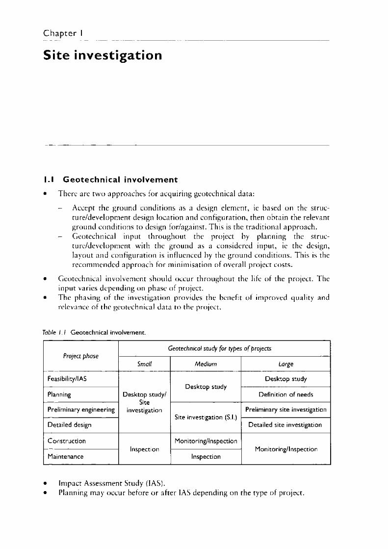
1.1 Geotechn ica l involvement• There are two approaches for acquiring geotechnical data:
Accept the ground conditions as a design element, ie based on the structure/development design location and configuration, then obtain the relevant ground conditions to design for/against. This is the traditional approach.
- Geotechnical input throughout the project by planning the structure/development with the ground as a considered input, ie the design,layout and configuration is influenced by the ground conditions. This is the recommended approach for minimisation of overall project costs.
• Geotechnical involvement should occur throughout the life of the project. The input varies depending on phase of project.
• The phasing of the investigation provides the benefit of improved quality andrelevance of the geotechnical data to the project.
Table 1.1 Geotechnical involvement.
Project phaseGeotechnical study for types o f projects
Small Medium Large
Feasibility/IAS
Desktop study/ Site
investigation
Desktop studyDesktop study
Planning Definition of needs
Preliminary engineeringSite investigation (S.l.)
Preliminary site investigation
Detailed design Detailed site investigation
ConstructionInspection
Monitoring/InspectionMonitoring/Inspection
Maintenance Inspection
• Impact Assessment Study (IAS).• Planning may occur before or after IAS depending on the type of project.
2 S ite invest igat io n
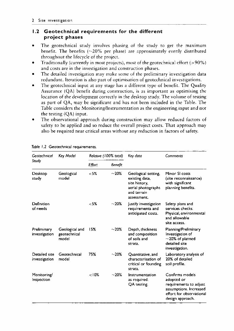
1.2 G eotechn ica l requ irem ents for the different pro ject phases
• The geotechnical study involves phasing of the study to get the maximum benefit. The benefits ( ^ 2 0 % per phase) are approximately evenly distributed throughout the lifecycle of the project.
• Traditionally (currently in most projects), most of the geotechnical effort ( > 9 0 % ) and costs are in the investigation and construction phases.
• The detailed investigation may make some of the preliminary investigation data redundant. Iteration is also part of optimisation of geotechnical investigations.
• The geotechnical input at any stage has a different type of benefit. The Quality Assurance (QA) benefit during construction, is as important as optimising the location of the development correctly in the desktop study. The volume of testing as part of QA, may be significant and has not been included in the Table. The Table considers the Monitoring/Instrumentation as the engineering input and not the testing (QA) input.
• The observational approach during construction may allow reduced factors of safety to be applied and so reduce the overall project costs. T hat approach may also be required near critical areas without any reduction in factors of safety.
Table 1.2 Geotechnical requirements.
GeotechnicalStudy
Key Model Relative (100% total)
Effort Benefit
Key data Comments
Desktopstudy
Geologicalmodel
<5% -20% Geological setting, existing data, site history, aerial photographs and terrain assessment.
Minor SI costs (site reconnaissance) with significant planning benefits.
Definition of needs
<5% -20% Justify investigation requirements and anticipated costs.
Safety plans and services checks. Physical, environmental and allowable site access.
Preliminaryinvestigation
Geological andgeotechnicalmodel
15% -20% Depth, thickness and composition of soils and strata.
Planning/Preliminary Investigation of —20% of planned detailed site investigation.
Detailed site investigation
Geotechnicalmodel
75% -20% Quantitative, and characterisation of critical or founding strata.
Laboratory analysis of 20% of detailed soil profile.
Monitoring/Inspection
<10% -20% Instrumentation as required.Q A testing.
Confirms models adopted orrequirements to adjust assumptions. Increased effort for observational design approach.
Site invest ig a t io n 3
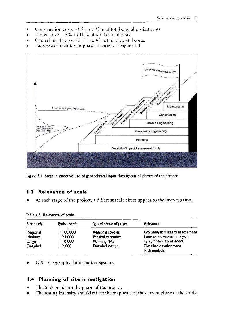
• Construction costs — 8 5 % to 9.5% of total capital project costs.• Design costs 5 % to 10% of total capital costs.• Geotechnical costs M) . I % to 4 % of total capital costs.• Kach peaks at different phase as shown in Figure 1.1.
[ 1
Figure 1.1 Steps in effective use of geotechnical input throughout all phases of the project.
1.3 Re levance of scale• At each stage of the project, a different scale effect applies to the investigation.
Table 1.3 Relevance of scale.
Size study Typical scale Typical phase o f project Relevance
Regional 1: 100,000 Regional studies GIS analysis/Hazard assessmentMedium 1:25,000 Feasibility studies Land units/Hazard analysisLarge 1: 10,000 Planning /IAS Terrain/Risk assessmentDetailed 1: 2,000 Detailed design Detailed development.
Risk analysis
• GIS - Geographic Information Systems
1.4 Planning of site investigation• The SI depends on the phase of the project.• The testing intensity should reflect the map scale of the current phase of the study.
4 S ite invest igat ion
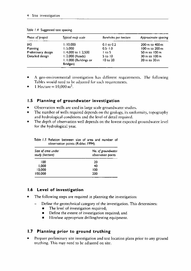
Table 1.4 Suggested test spacing.
Phase o f project Typical map scale Boreholes per hectare Approximate spacing
IAS 1: 10,000 0.1 to 0.2 200 m to 400 mPlanning 1:5,000 0.5-1.0 100 m to 200 mPreliminary design 1:4,000 to 1: 2,500 1 to 5 50 m to 100 mDetailed design 1:2,000 (Roads) 5 to 10 30 m to 100 m
1: 1,000 (Buildings or Bridges)
10 to 20 20 m to 30 m
• A geo-environmental investigation has different requirements. The following Tables would need to be adjusted for such requirements.
• 1 Hectare = 10 ,000 m2.
1.5 Planning of groundwater investigation• Observation wells are used in large scale groundwater studies.• The number of wells required depends on the geology, its uniformity, topography
and hydrological conditions and the level of detail required.• The depth of observation well depends on the lowest expected groundwater level
for the hydrological year.
Table 1.5 Relation between size of area and number of observation points (Ridder, 1994).
Size o f area under study (hectare)
No. o f groundwater observation points
100 201,000 40
10,000 100100,000 200
1.6 Level of investigation• The following steps are required in planning the investigation:
- Define the geotechnical category of the investigation. This determines:■ The level of investigation required;■ Define the extent of investigation required; and■ Hire/use appropriate drilling/testing equipment.
1.7 Planning prior to ground truthing• Prepare preliminary site investigation and test location plans prior to any ground
truthing. This may need to be adjusted on site.
Site in vest ig a t io n 5
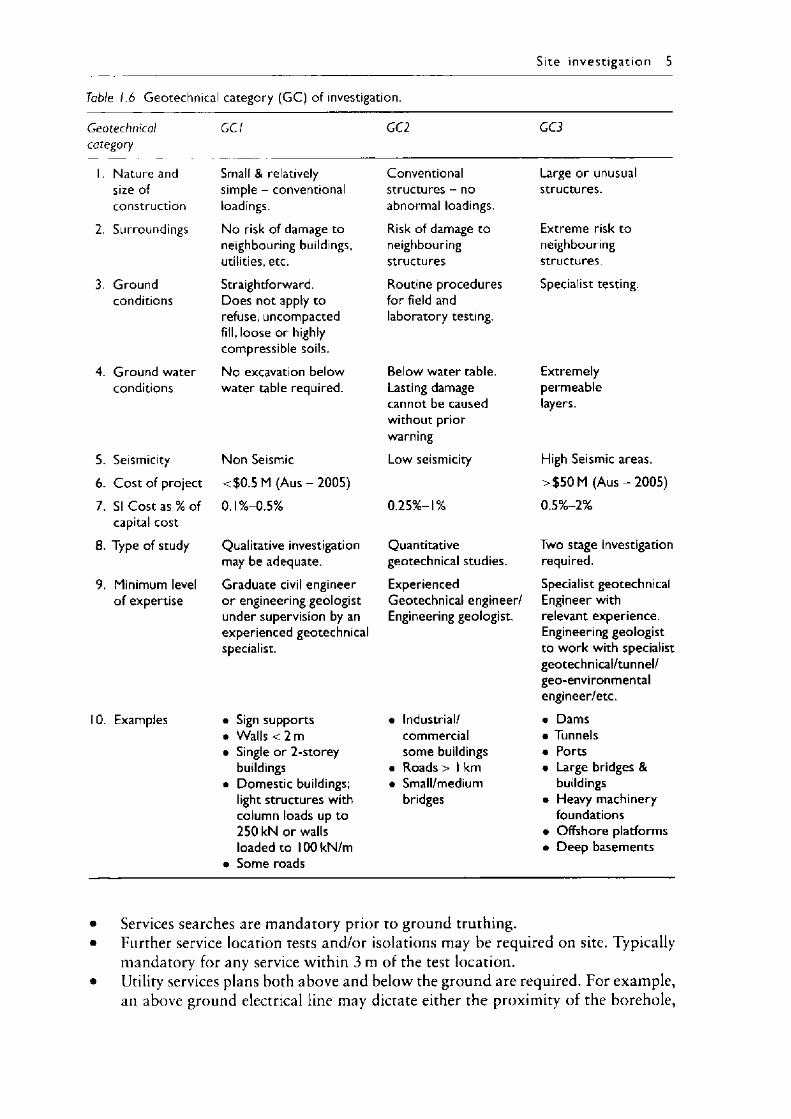
Table 1.6 Geotechnical category (G C) of investigation.
Geotechnicalcategory
C C I C C I CC3
1. Nature and Small & relatively Conventional Large or unusualsize of simple - conventional structures - no structures.construction loadings. abnormal loadings.
2. Surroundings No risk of damage to Risk of damage to Extreme risk toneighbouring buildings, neighbouring neighbouringutilities, etc. structures structures.
3. Ground Straightforward. Routine procedures Specialist testing.conditions Does not apply to
refuse, uncompacted fill, loose or highly compressible soils.
for field and laboratory testing.
4. Ground water No excavation below Below water table. Extremelyconditions water table required. Lasting damage
cannot be caused without prior warning
permeablelayers.
5. Seismicity Non Seismic Low seismicity High Seismic areas.6. Cost of project < $0.5 M (A u s- 2005) >$50 M (A u s- 2005)
7. SI Cost as % of capital cost
0.1 %—0.5% 0.25%-1% 0.5%-2%
8. Type of study Qualitative investigation Quantitative Two stage investigationmay be adequate. geotechnical studies. required.
9. Minimum level Graduate civil engineer Experienced Specialist geotechnicalof expertise or engineering geologist Geotechnical engineer/ Engineer with
under supervision by an experienced geotechnical specialist.
Engineering geologist. relevant experience. Engineering geologist to work with specialist geotechnical/tunnel/ geo-environmental engineer/etc.
10. Examples • Sign supports • Industrial/ • Dams• Walls < 2 m commercial • Tunnels• Single or 2-storey some buildings • Ports
buildings • Roads > 1 km • Large bridges &• Domestic buildings; • Small/medium buildings
light structures with column loads up to 250 kN or walls loaded to 100 kN/m
• Some roads
bridges • Heavy machinery foundations
• Offshore platforms• Deep basements
• Services searches are mandatory prior to ground truthing.• Further service location tests and/or isolations may be required on site. Typically
mandatory for any service within 3 m of the test location.• Utility services plans both above and below the ground are required. For example,
an above ground electrical line may dictate either the proximity of the borehole,
6 S ite investigat ion
or a drilling rig with a certain mast height and permission from the electrical safety authority before proceeding.The planning should allow for any physical obstructions such as coring of a concrete slab, and its subsequent repair after coring.
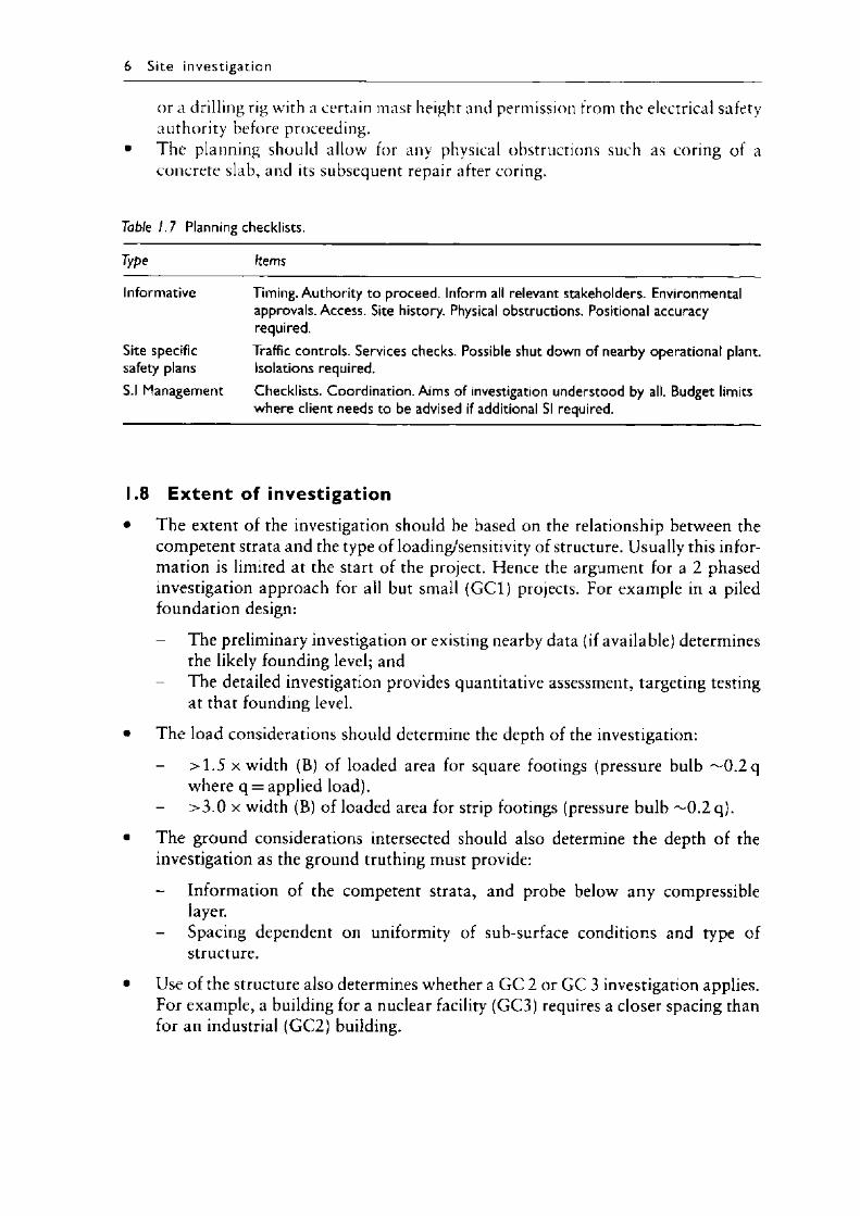
Table 1.7 Planning checklists.
Type Items
Informative Timing. Authority to proceed. Inform all relevant stakeholders. Environmentalapprovals. Access. Site history. Physical obstructions. Positional accuracy required.
Site specific Traffic controls. Services checks. Possible shut down of nearby operational plant.safety plans Isolations required.S.I Management Checklists. Coordination. Aims of investigation understood by all. Budget limits
where client needs to be advised if additional SI required.
1.8 E x ten t of investigation• The extent of the investigation should be based on the relationship between the
competent strata and the type of loading/sensitivity of structure. Usually this information is limited at the start of the project. Hence the argument for a 2 phased investigation approach for all but small (GC1) projects. For example in a piled foundation design:
- The preliminary investigation or existing nearby data (if available) determines the likely founding level; and
- The detailed investigation provides quantitative assessment, targeting testing at that founding level.
• The load considerations should determine the depth of the investigation:
- > 1 . 5 x width (B) of loaded area for square footings (pressure bulb ~ 0 . 2 q where q = applied load).
- > 3 . 0 x width (B) of loaded area for strip footings (pressure bulb ~ 0 . 2 q ) .
• The ground considerations intersected should also determine the depth of the investigation as the ground truthing must provide:
- Information of the competent strata, and probe below any compressible layer.
- Spacing dependent on uniformity of sub-surface conditions and type of structure.
• Use of the structure also determines whether a GC 2 or GC 3 investigation applies. For example, a building for a nuclear facility (GC3) requires a closer spacing than for an industrial (GC2) building.
Site invest ig a t io n 7
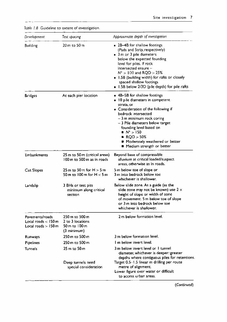
Table 1.8 Guideline to extent of investigation.
Development Test spacing Approximate depth o f investigation
Building 20 m to 50 m • 2B-4B for shallow footings (Pads and Strip, respectively)
• 3 m or 3 pile diameters below the expected founding level for piles. If rock intersected ensure -N* > 100 and R Q D > 25%
• I.5B (building width) for rafts or closely spaced shallow footings
• 1.5B below 2/3D (pile depth) for pile rafts
Bridges At each pier location • 4B-5B for shallow footings• 10 pile diameters in competent
strata, or• Consideration of the following if
bedrock intersected- 3 m minimum rock coring - 3 Pile diameters below target
founding level based on■ N* > 150■ R Q D >50%■ Moderately weathered or better■ Medium strength or better
Embankments 25 m to 50 m (critical areas) 100 m to 500 m as in roads
Beyond base of compressiblealluvium at critical loaded/suspect areas, otherwise as in roads.
Cut Slopes 25 m to 50 m for H > 5 m 50 m to 100 m for H < 5 m
5 m below toe of slope or 3 m into bedrock below toe
whichever is shallower.Landslip 3 BHs or test pits
minimum along critical section
Below slide zone. As a guide (as the slide zone may not be known) use 2 x height of slope or width of zone of movement. 5 m below toe of slope or 3 m into bedrock below toe whichever is shallower.
Pavements/roads Local roads < 150 m Local roads > 150 m
RunwaysPipelinesTunnels
250 m to 500 m 2 to 3 locations 50 m to 100 m (3 minimum)250 m to 500 m250 m to 500 m25 m to 50 m
Deep tunnels need special consideration
2 m below formation level.
3 m below formation level.I m below invert level.3 m below invert level or I tunnel
diameter, whichever is deeper: greater depths where contiguous piles for retentions.
Target 0 .5 -1.5 linear m drilling per route metre of alignment.
Lower figure over water or difficult to access urban areas.
(Continued)
8 S ite invest igat io n
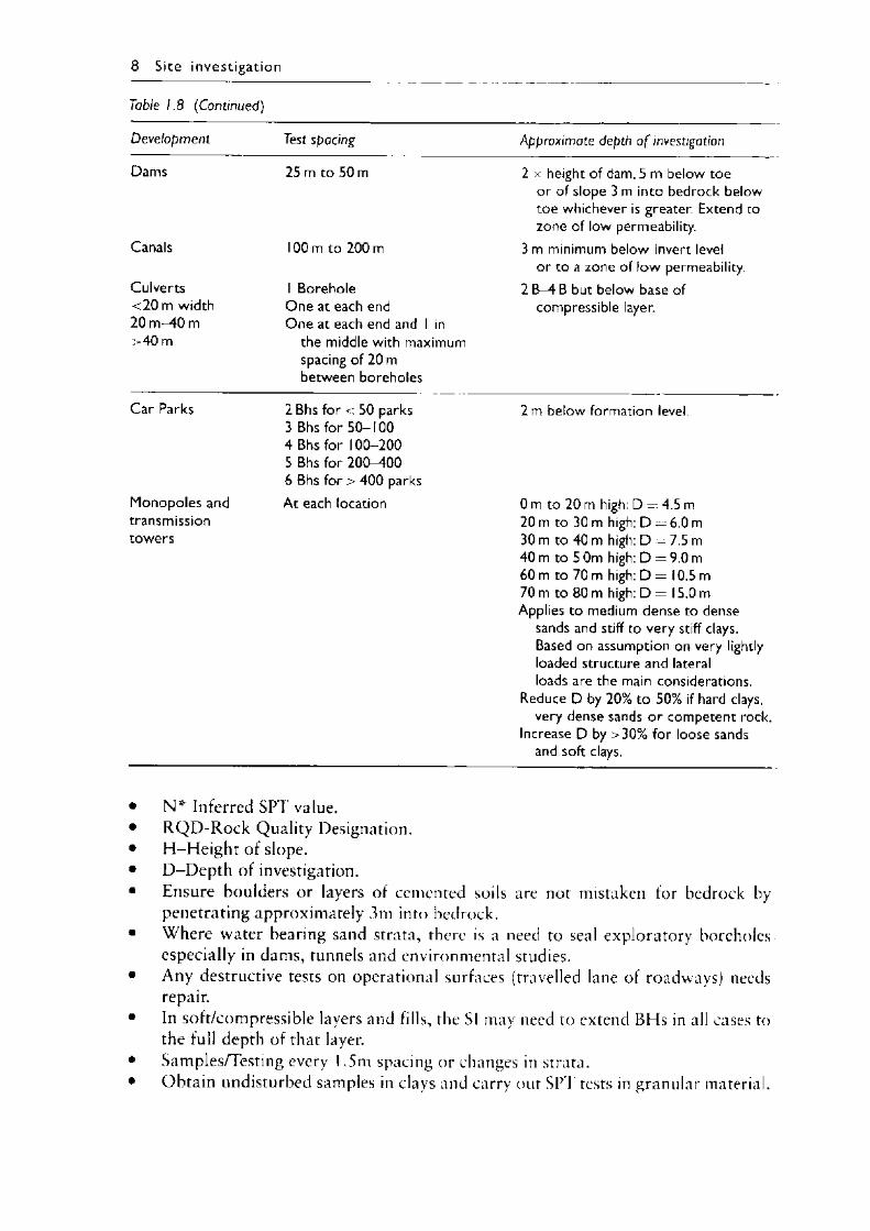
Table 1.8 (Continued)
Development Test spacing Approximate depth o f investigation
Dams 25 m to 50 m 2 x height of dam, 5 m below toe or of slope 3 m into bedrock below toe whichever is greater. Extend to zone of low permeability.
Canals 100 m to 200 m 3 m minimum below invert level or to a zone of low permeability.
Culverts 1 Borehole 2 B-4 B but below base of< 2 0 m width One at each end compressible layer.20 m -40 m One at each end and 1 in>40 m the middle with maximum
spacing of 20 m between boreholes
Car Parks 2 Bhs for < 50 parks3 Bhs for 50-1004 Bhs for 100-2005 Bhs for 200-4006 Bhs for > 400 parks
2 m below formation level.
Monopoles and At each location 0 m to 20 m high: D = 4.5 mtransmission 20 m to 30 m high: D — 6.0 mtowers 30 m to 40 m high: D — 7.5 m
40 m to 5 0m high: D = 9.0 m 60 m to 70 m high: D = 10.5 m 70 m to 80 m high: D = 1 5.0 m Applies to medium dense to dense
sands and stiff to very stiff clays. Based on assumption on very lightly loaded structure and lateral loads are the main considerations.
Reduce D by 20% to 50% if hard clays, very dense sands or competent rock.
Increase D by >30% for loose sands and soft clays.
• N * Inferred SPT value.• R Q D - R o c k Quality Designation.• H-H eig ht of slope.• D -D e p th of investigation.• Ensure boulders or layers of cemented soils are not mistaken for bedrock by
penetrating approximately 3m into bedrock.• Where water bearing sand strata, there is a need to seal exploratory boreholes
especially in dams, tunnels and environmental studies.• Any destructive tests on operational surfaces (travelled lane of roadways) needs
repair.• In soft/compressible layers and fills, the SI may need to extend BHs in all cases to
the full depth of that layer.• Samples/Testing every 1.5m spacing or changes in strata.• Obtain undisturbed samples in clays and carry out SPT tests in granular material.
Site in ves t ig a t io n 9
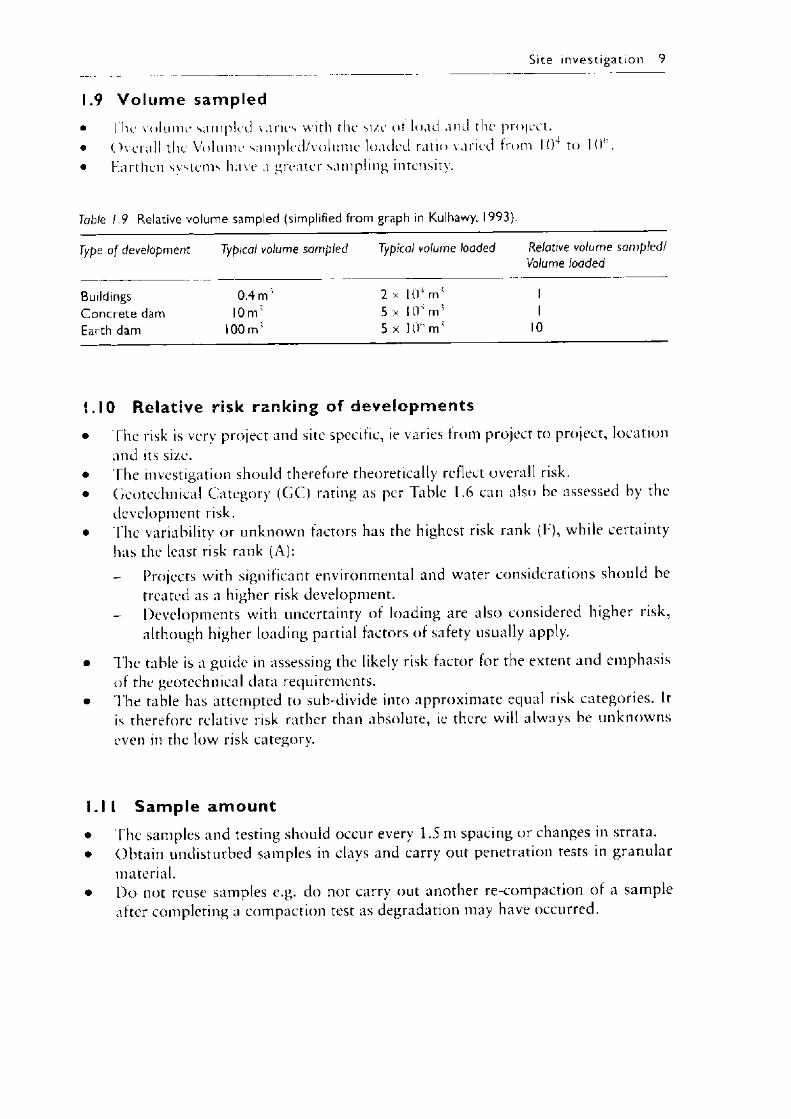
1.9 V o l u m e sampled• Ihe volume sampled vanes with the si/e of load and the project.• Overall the Volume sampled/volume loaded ratio varied from 104 to 10* .• Harthen systems have a greater sampling intensity.
Table 1.9 Relative volume sampled (simplified from graph in Kulhawy, 1993).
Type o f development Typical volume sampled Typical volume loaded Relative volume sampled/ Volume loaded
Buildings 0.4 m ' 2 x I0 4 m' 1Concrete dam 10 m 1 5 x 1 0 'm ’ 1Earth dam 100 m ' 5 x 10 h m 1 10
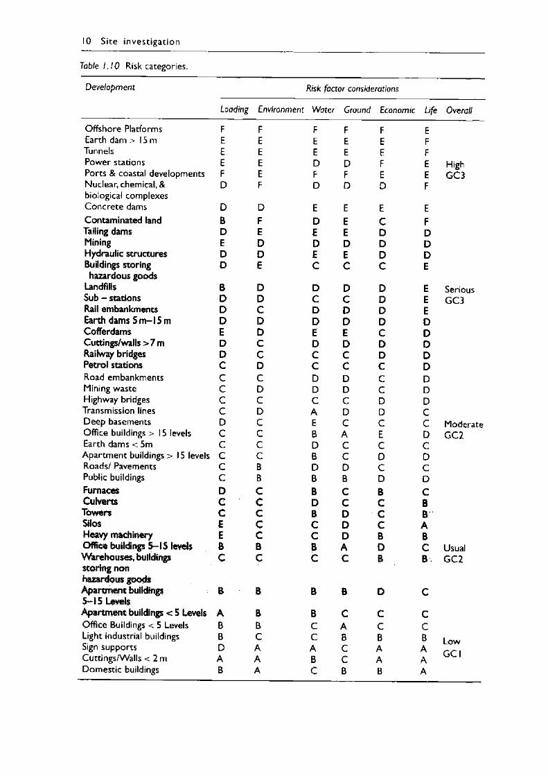
1.10 Relative risk ranking of developments• The risk is very project and site specific, ie varies from project to project, location
and its size.• The investigation should therefore theoretically reflect overall risk.• Geotechnical Category (GC) rating as per Table 1.6 can also be assessed by the
development risk.• The variability or unknown factors has the highest risk rank (F), while certainty
has the least risk rank (A):
- Projects with significant environmental and water considerations should be treated as a higher risk development.
- Developments with uncertainty of loading are also considered higher risk, although higher loading partial factors of safety usually apply.
• The table is a guide in assessing the likely risk factor for the extent and emphasis of the geotechnical data requirements.
• The table has attempted to sub-divide into approximate equal risk categories. It is therefore relative risk rather than absolute, ie there will always be unknowns even in the low risk category.
1.1 I Sample amount• The samples and testing should occur every 1.5 m spacing or changes in strata.• Obtain undisturbed samples in clays and carry out penetration tests in granular
material.• Do not reuse samples e.g. do not carry out another re-compaction of a sample
after completing a compaction test as degradation may have occurred.
10 S ite invest igat ion
Tab let. 10 Risk categories.
Development Risk factor considerations
Loading Environment Water Ground Economic Life Overall
Offshore Platforms F F F F F EEarth dam > 15 m E E E E E FTunnels E E E E E FPower stations E E D D F E HighPorts & coastal developments F E F F E E G C3Nuclear, chemical, & biological complexes
D F D D D F
Concrete dams D D E E E EContaminated land B F D E C FTailing dams D E E E D DMining E D D D D DHydraulic structures D D E E D DBuildings storing hazardous goods
D E C C C E
Landfills B D D D D E SeriousSub - stations D D C C D E G C3Rail embankments D C D D D EEarth dams 5m -l5m D D D D D DCofferdams E D E E C DCuttings/walls >7 m D C D D D DRailway bridges D C C C D DPetrol stations C D C C C DRoad embankments C C D D C DMining waste C D D D c DHighway bridges c C C C D DTransmission lines c D A D D CDeep basements D C E C C C ModerateOffice buildings > 15 levels C C B A E D G C 2Earth dams < 5m C C D C C CApartment buildings > 15 levels C C B C D DRoads/ Pavements C B D D C CPublic buildings C B B B D DFurnaces D C B C B CCulverts C C D C C BTowers C C B D C BSilos E c C D C AHeavy machinery E c C D B BOffice buildings 5-15 levels B B B A D C UsualWarehouses, buildings storing non hazardous goods
C c C C B B G C 2
Apartment buildings 5-15 Levels
B B B B D C
Apartment buildings < 5 Levels A B B C C COffice Buildings < 5 Levels B B C A C CLight industrial buildings B C c B B B LowSign supports D A A C A A G C ICuttings/Walls < 2 m A A B C A ADomestic buildings B A C B B A
Site invest iga t ion I I
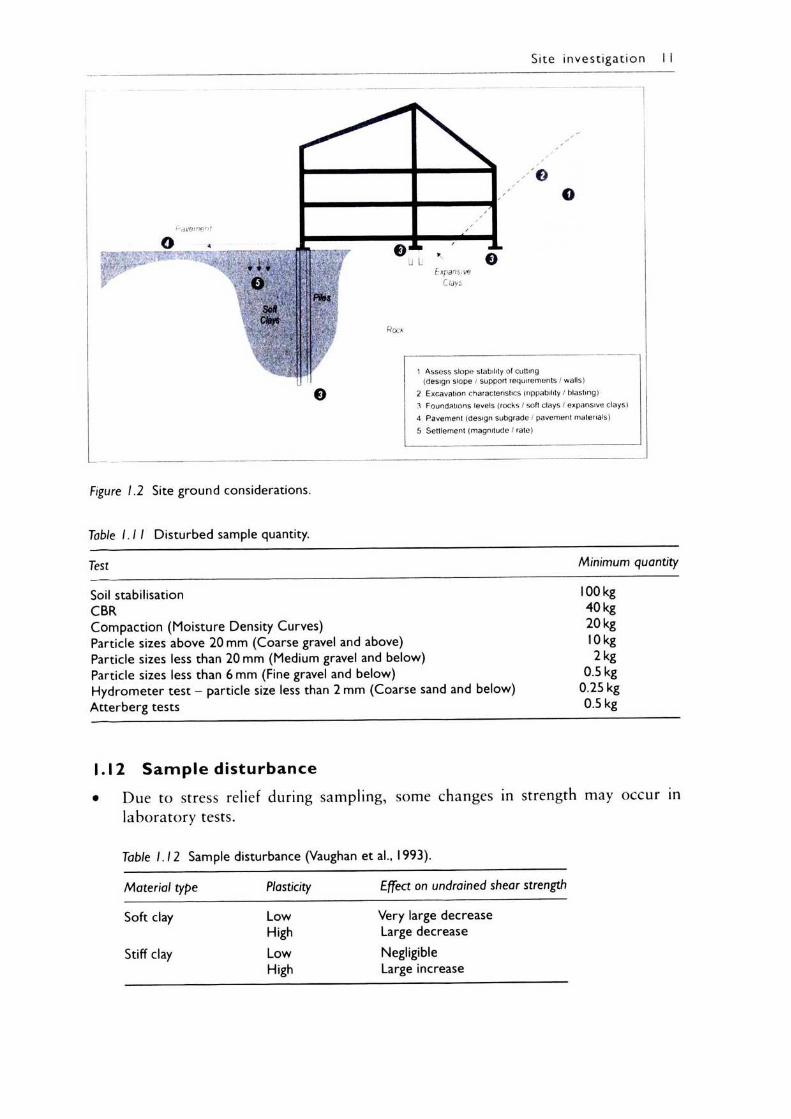
F&E&.
1 Assess slope stability of cutting(design slope / support requirements / walls)
2 Excavation characteristics (rippability / blasting)3 Foundations levels (rocks / soft clays / expansive clays)4 Pavement (design subgrade / pavement materials)5 Settlement (magnitude / rate)
Figure 1.2 Site ground considerations.
Table 1.11 Disturbed sample quantity.
Test Minimum quantity
Soil stabilisation 100 kgCBR 40 kgCompaction (Moisture Density Curves) 20 kgParticle sizes above 20 mm (Coarse gravel and above) 10 kgParticle sizes less than 20 mm (Medium gravel and below) 2 kgParticle sizes less than 6 mm (Fine gravel and below) 0.5 kgHydrometer test - particle size less than 2 mm (Coarse sand and below) 0.25 kgAtterberg tests 0.5 kg
1.12 Sam p le disturbance• Due to stress relief during sampling, some changes in strength may occur in
laboratory tests.
Table 1.12 Sample disturbance (Vaughan et al., 1993).
Material type Plasticity Effect on undrained shear strength
Soft clay Low Very large decreaseHigh Large decrease
Stiff clay Low NegligibleHigh Large increase
12 S ite investigat ion
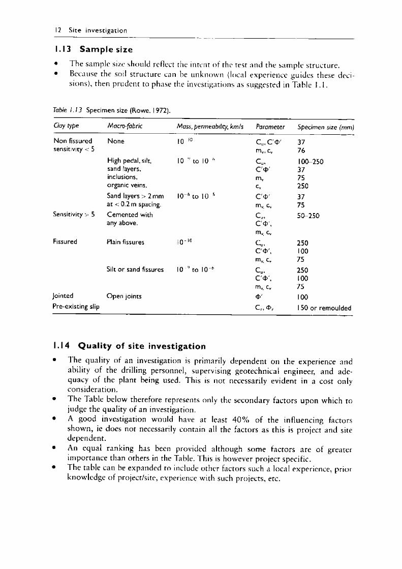
1.13 Sam ple size• The sample size should reflect the intent of the test and the sample structure.• Because the soil structure can be unknown (local experience guides these deci
sions), then prudent to phase the investigations as suggested in Table 1.1.
Table 1.13 Specimen size (Rowe, 1972).
Clay type Macro-fabric Moss, permeability, km/s Parameter Specimen size (mm)
Non fissured None 10 10 C u, C'<t>' 37sensitivity < 5 mv, cv 76
High pedal, silt, 10 'to 10 6 C ut 100-250sand layers. C4>' 37inclusions. mv 75organic veins. cv 250Sand layers > 2 mm 10 6 to 10 5 C O ' 37at < 0.2 m spacing. mv. cv 75
Sensitivity > 5 Cemented with Q , 50-250any above. C'<D\
mv cvFissured Plain fissures 10 10 C u, 250
c o \ 100mv cv 75
Silt or sand fissures 10 9 to 10 6 Cu. 250C O , 100mv. cv 75
Jointed Open joints O' 100Pre-existing slip c r, o r 1 50 or remoulded
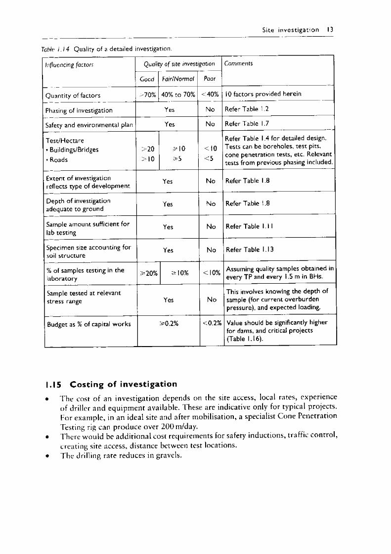
1.14 Qua l ity of site investigation• The quality of an investigation is primarily dependent on the experience and
ability of the drilling personnel, supervising geotechnical engineer, and adequacy of the plant being used. This is not necessarily evident in a cost only consideration.
• The Table below therefore represents only the secondary factors upon which to judge the quality of an investigation.
• A good investigation would have at least 4 0 % of the influencing factors shown, ie does not necessarily contain all the factors as this is project and site dependent.
• An equal ranking has been provided although some factors are of greater importance than others in the Table. This is however project specific.
• The table can be expanded to include other factors such a local experience, prior knowledge of project/site, experience with such projects, etc.
Site invest ig a t io n 13
Table 1.14 Quality of a detailed investigation.
Influencing factors Qualit
Good
y o f site invest
Fair/Normal
gation
Poor
Comments
Quantity of factors >70% 40% to 70% <40% 10 factors provided herein
Phasing of investigation Yes No Refer Table 1.2
Safety and environmental plan Yes No Refer Table 1.7
Test/Hectare• Buildings/Bridges• Roads
>20>10
5=10^5
<10<5
Refer Table 1.4 for detailed design. Tests can be boreholes, test pits, cone penetration tests, etc. Relevant tests from previous phasing included.
Extent of investigation reflects type of development Yes No Refer Table 1.8
Depth of investigation adequate to ground
Yes No Refer Table 1.8
Sample amount sufficient for lab testing
Yes No Refer Table 1.1 1
Specimen size accounting for soil structure
Yes No Refer Table 1.13
% of samples testing in the laboratory
^20% 5=10% <10% Assuming quality samples obtained in every TP and every 1.5 m in BHs.
Sample tested at relevant stress range Yes No
This involves knowing the depth of sample (for current overburden pressure), and expected loading.
Budget as % of capital works ^0.2% <0.2% Value should be significantly higher for dams, and critical projects (Table 1.16).
1.15 Cost ing of investigation• The cost of an investigation depends on the site access, local rates, experience
of driller and equipment available. These are indicative only for typical projects. For example, in an ideal site and after mobilisation, a specialist Cone Penetration Testing rig can produce over 2 0 0 m/day.
• There would be additional cost requirements for safety inductions, traffic control, creating site access, distance between test locations.
• The drilling rate reduces in gravels.
14 S ite invest igat ion
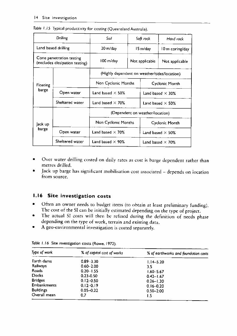
Table 1.15 Typical productivity for costing (Queensland Australia).
Drilling Soil Soft rock Hard rock
Land based drilling 20 m/da/ 15 m/day 10 m coring/day
Cone penetration testing (excludes dissipation testing) 100 m/day Not applicable Not applicable
Floatingbarge
(Highly dependent on weather/tides/location)
Non Cyclonic Months Cyclonic Month
Open water Land based X 50% Land based X 30%
Sheltered water Land based X 70% Land based X 50%
Jack up barge
(Dependent on weather/location)
Non Cyclonic Months Cyclonic Month
Open water Land based X 70% Land based X 50%
Sheltered water Land based X 90% Land based X 70%
• Over water drilling costed on daily rates as cost is barge dependent rather than metres drilled.
• Jack up barge has significant mobilisation cost associated - depends on location from source.
1.16 S ite investigation costs• Often an owner needs to budget items (to obtain at least preliminary funding).
The cost of the SI can be initially estimated depending on the type of project.• The actual SI costs will then be refined during the definition of needs phase
depending on the type of work, terrain and existing data.• A geo-environmental investigation is costed separately.
Table 1.16 Site investigation costs (Rowe, 1972).
Type o f work % o f capital cost o f works % o f earthworks and foundation costs
Earth dams 0.89-3.30 1.14-5.20Railways 0.60-2.00 3.5Roads 0.20-1.55 1.60-5.67Docks 0.23-0.50 0.42-1.67Bridges 0.12-0.50 0.26-1.30Embankments 0.12-0.19 0.16-0.20Buildings 0.05-0.22 0.50-2.00Overall mean 0.7 1.5
• Overall the % values for buildings seem low and assume some prior knowledge of the site.
• A value of 0 . 2 % of capital works should be the minimum budgeted for sufficient information.
• The laboratory testing for a site investigation is typically 10% to 2 0 % of the testing costs, while the field investigation is the remaining 8 0 % to 9 0 % , but this varies depending on site access. This excludes the professional services of supervision and reporting. There is an unfortunate trend to reduce the laboratory testing, with inferred properties from the visual classification and/or field testing only.
1.17 T he business of site investigation• The geotechnical business can be divided into 3 parts (professional, field and
laboratory).• Each business can be combined, ie consultancy with laboratory, or exploratory
with laboratory testing:
There is an unfortunate current trend to reduce the laboratory testing, and base the recommended design parameters on typical values based on field soil classifications. This is a commercial/ competitive bidding decision rather than the best for project/optimal geotechnical data. It also takes away the field/laboratory check essential for calibration of the field assessment and for the development and training of geotechnical engineers.
Site invest ig a t io n 15
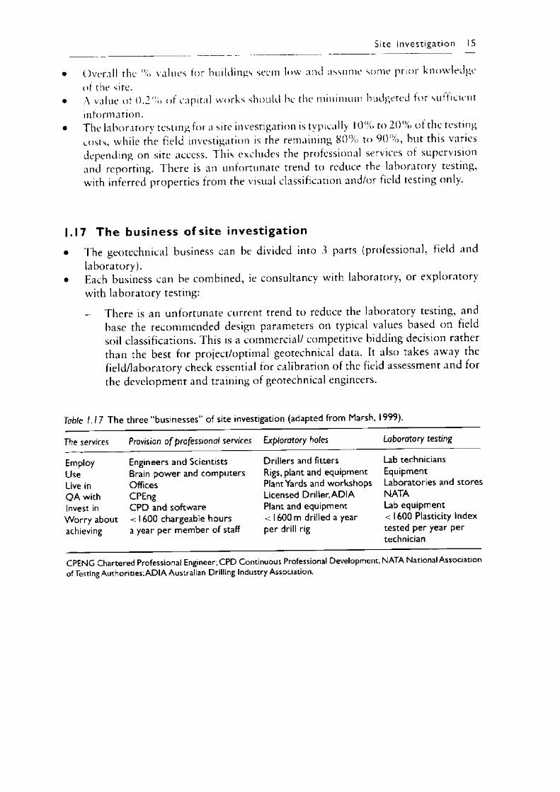
Table 1.17 The three “businesses” of site investigation (adapted from Marsh, 1999).
The services Provision o f professional services Exploratory holes Laboratory testing
Employ Use Live in Q A with Invest in W orry about achieving
Engineers and Scientists Brain power and computers Offices CPEngCPD and software < 1600 chargeable hours a year per member of staff
Drillers and fitters Rigs, plant and equipment Plant Yards and workshops Licensed Driller,ADIA Plant and equipment < 1600 m drilled a year per drill rig
Lab technicians EquipmentLaboratories and stores NATALab equipment < 1600 Plasticity Index tested per year per technician
C P E N G Ch artered Professional Engineer; C P D Continuous Professional Developm ent; N A TA National Association of Testing Authorities; A D IA Australian Drilling Industry Association.

Chapter 2
Soil classification
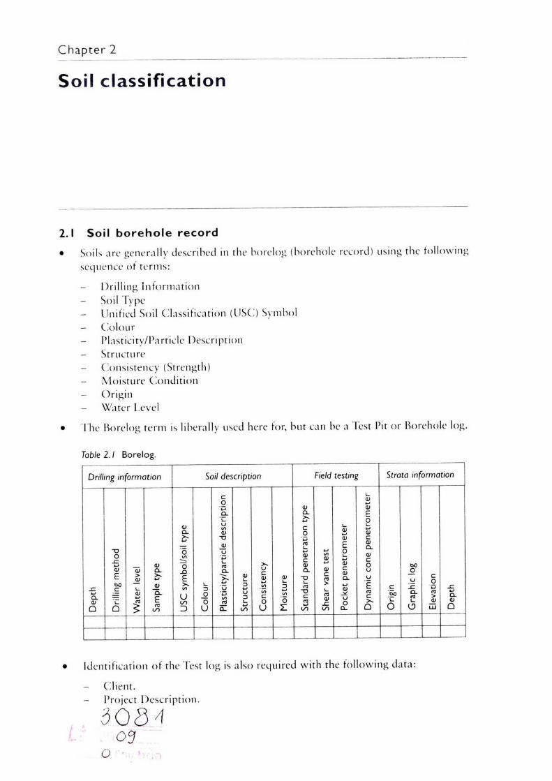
2.1 Soil borehole record• Soils arc generally described in the borelog (borehole record) using the following
sequence of terms:
- Drilling Information- Soil Type
Unified Soil Classification (USC) Symbol- Colour- Plasticity/Particle Description- Structure
Consistency (Strength)Moisture Condition
- Origin- Water Level
• The Borelog term is liberally used here for, but can be a Test Pit or Borehole log.
Table 2 .1 Borelog.
Drilling information Soil description Field testing Strata information
Dept
h
Drilli
ng
met
hod
Wat
er
level
Samp
le typ
e J
USC
sym
bol/s
oil
type
Colo
ur
Plas
ticity
/par
ticle
desc
riptio
n
Stru
ctur
e
Cons
isten
cy
Moi
stur
e
Stand
ard
pene
tratio
n ty
pe
Shea
r van
e te
st
Pock
et p
enet
rom
eter
Dyna
mic
cone
pe
netro
met
er
Orig
in
Grap
hic
log
Eleva
tion
Dept
h
• Identification of the Test log is also required with the following data:
Client.Project Description.
3 0 3 ^ 1
o
18 So il c la ss i f ica t ion
- Project Location.Project Number.Sheet No. - ofReference: Easting, Northing, Elevation, Inclination.
- Date started and completed.- Geomechanical details only. Environmental details not covered.
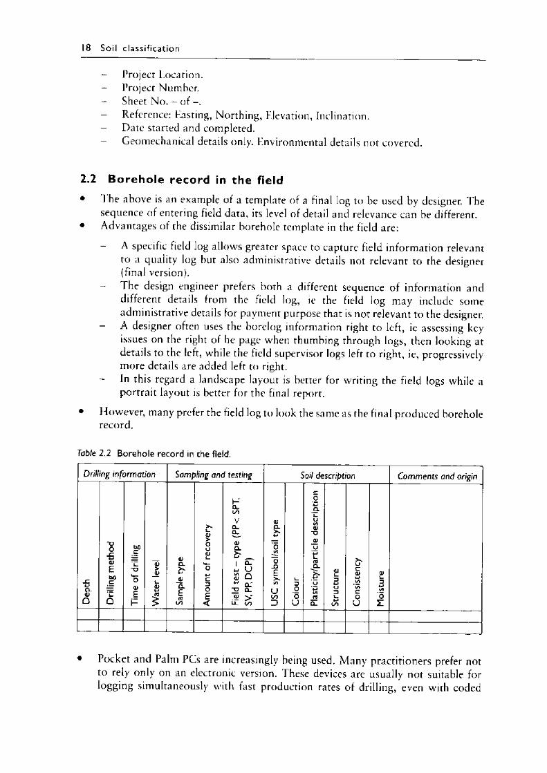
2.2 Borehole record in the field• The above is an example of a template of a final log to be used by designer. The
sequence of entering field data, its level of detail and relevance can be different.• Advantages of the dissimilar borehole template in the field are:
- A specific field log allows greater space to capture field information relevant to a quality log but also administrative details not relevant to the designer (final version).
- The design engineer prefers both a different sequence of information and different details from the field log, ie the field log may include some administrative details for payment purpose that is not relevant to the designer.
- A designer often uses the borelog information right to left, ie assessing key issues on the right of he page when thumbing through logs, then looking at details to the left, while the field supervisor logs left to right, ie, progressively more details are added left to right.
- In this regard a landscape layout is better for writing the field logs while a portrait layout is better for the final report.
• However, many prefer the field log to look the same as the final produced borehole record.
Table 2.2 Borehole record in the field.
Drilling information Sampling and testing Soil description Comments and origin
Dept
h
Drilli
ng
met
hod
Time
of dr
illing
Wat
er l
evel
Samp
ie ty
pe
Amou
nt o
f re
cove
ry
Field
test
- typ
e (PP
< SP
T, SV
, PP.
DCP)
USC
sym
bol/s
oil t
ype
Colo
ur
Plas
ticity
/par
ticle
desc
riptio
n
Stru
ctur
e
Cons
isten
cy
Moi
stur
e
• Pocket and Palm PCs are increasingly being used. Many practitioners prefer not to rely only on an electronic version. These devices are usually not suitable for logging simultaneously with fast production rates of drilling, even with coded
Soil c la ss i f ica t io n 19
entries. These devices are useful in mapping cuttings and for relatively slow rock coring on site, or for cores already drilled.
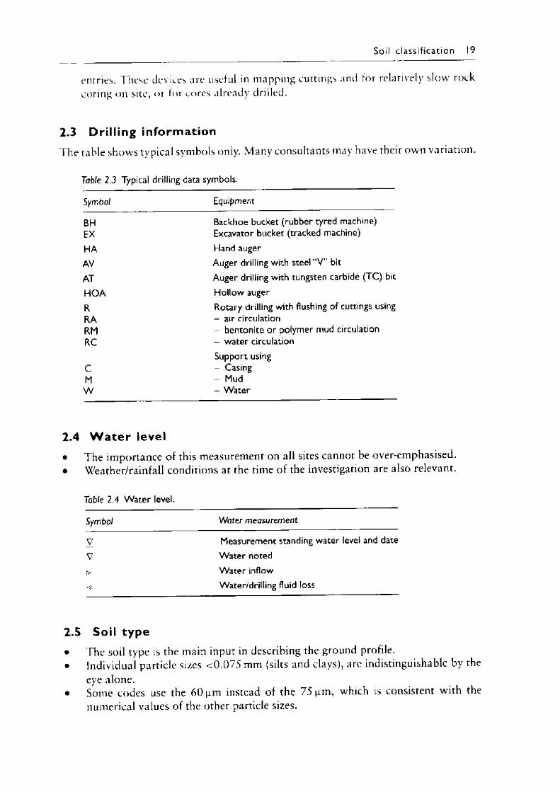
2.3 Dri l ling informationThe table shows t y p i c a l symbols only. Many consultants may have their own variation.
Table 2.3 Typical drilling data symbols.
Symbol Equipment
BH Backhoe bucket (rubber tyred machine)EX Excavator bucket (tracked machine)HA Hand augerAV Auger drilling with steel “V” bitAT Auger drilling with tungsten carbide (TC) bitH O A Hollow augerR Rotary drilling with flushing of cuttings usingRA - air circulationRM - bentonite or polymer mud circulationRC - water circulation
Support usingC - CasingM - MudW - Water
2.4 W a t e r level• The importance of this measurement on all sites cannot be over-emphasised.• Weather/rainfall conditions at the time of the investigation are also relevant.
Table 2.4 W ater level.
Symbol Water measurement
V Measurement standing water level and dateV W ater noted> W ater inflow<1 Water/drilling fluid loss
2.5 Soil type• The soil type is the main input in describing the ground profile.• Individual particle sizes < 0 .0 7 5 mm (silts and clays), are indistinguishable by the
eye alone.• Some codes use the 6 0 urn instead of the 75 nm, which is consistent with the
numerical values of the other particle sizes.
20 So il c la ss i f ica t io n
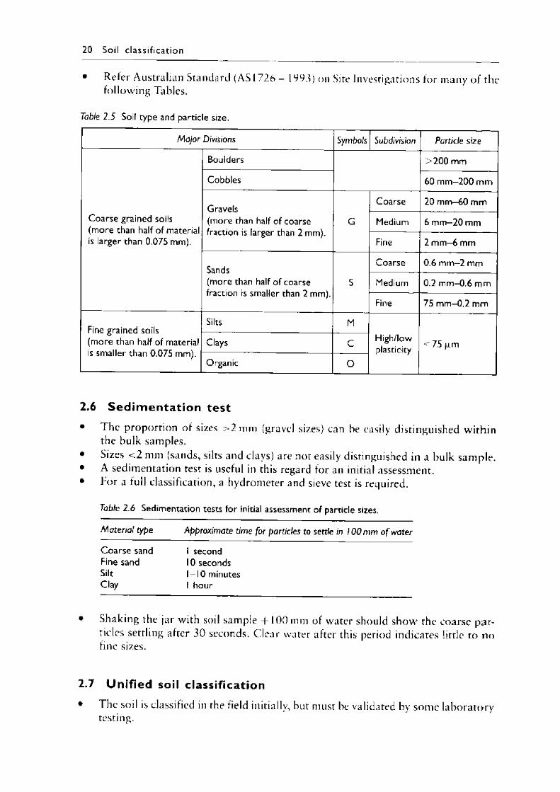
• Refer Australian Standard (AS I 26 - 1993) on Site Investigations for many of the following Tables.
Table 2.5 Soil type and particle size.
Major Divisions Symbols Subdivision Particle size
Boulders >200 mm
Cobbles 60 mm-200 mm
GravelsCoarse 20 mm—60 mm
Coarse grained soils (more than half of material is larger than 0.075 mm).
(more than half of coarse fraction is larger than 2 mm).
G Medium 6 mm-20 mm
Fine 2 mm-6 mm
SandsCoarse 0.6 mm-2 mm
(more than half of coarse fraction is smaller than 2 mm).
S Medium 0.2 mm-0.6 mm
Fine 75 mm—0.2 mm
Fine grained soils (more than half of material is smaller than 0.075 mm).
Silts M
Clays C High/lowplasticity <75 |im
Organic O
2.6 Sed im entat ion test• I he proportion of sizes > 2 mm (gravel sizes) can be easily distinguished within
the bulk samples.• Sizes < 2 mm (sands, silts and clays) are not easily distinguished in a bulk sample.• A sedimentation test is useful in this regard for an initial assessment.• For a full classification, a hydrometer and sieve test is required.
Table 2.6 Sedimentation tests for initial assessment of particle sizes.
Material type Approximate time for particles to settle in 100 mm o f water
Coarse sand 1 secondFine sand 10 secondsSilt 1 —10 minutesClay 1 hour
• Shaking the jar with soil sample + 1 0 0 mm of water should show the coarse particles settling after 30 seconds. Clear water after this period indicates little to no fine sizes.
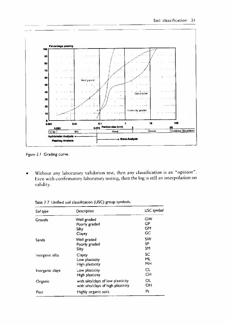
2.7 Unified soil classification• The soil is classified in the field initially, but must be validated by some laboratory
testing.
Soil c la s s i f ic a t io n 21
Percentage passing
90
80
70
60
50
40
30
20
10
100
0 0.001
0.002Clay
0.01
SiltHydrometer Analysis
Plasticty Analysis
j
- / ......... ■ - y * ....... /
s \ - ........../
Well gradedAy .........
/ / y
//y
■ Y .........
— j - b V j l / 'Gap graded
y )
L j T r Uniformly gradedp n 7i
0.1 1
0 075 Particie size (mm)
10
Sand Graval
Sieve Analysis
10060
Cobbles Boulders
Figure 2 .1 Grading curve.
Without any laboratory validation test, then any classification is an “opinion”. Even with confirmatory laboratory testing, then the log is still an interpolation on validity.
Table 2.7 Unified soil classification (USC) group symbols.
Soil type Description USC symbol
Gravels Well graded G WPoorly graded GPSilty GMClayey G C
Sands Well graded SWPoorly graded SPSilty SM
Inorganic silts Clayey SCLow plasticity MLHigh plasticity MH
Inorganic clays Low plasticity C LHigh plasticity CH
Organic with silts/clays of low plasticity O Lwith silts/clays of high plasticity OH
Peat Highly organic soils Pt
22 So il c la s s i f ic a t io n
• Laboratory testing is essential in borderline cases, eg silty sand vs sandy silt.
- Once classified many inferences on the behaviour and use of the soil is made.- Medium Plasticity uses symbols mixed or intermediate symbols eg CL/CH or
Cl (Intermediate).
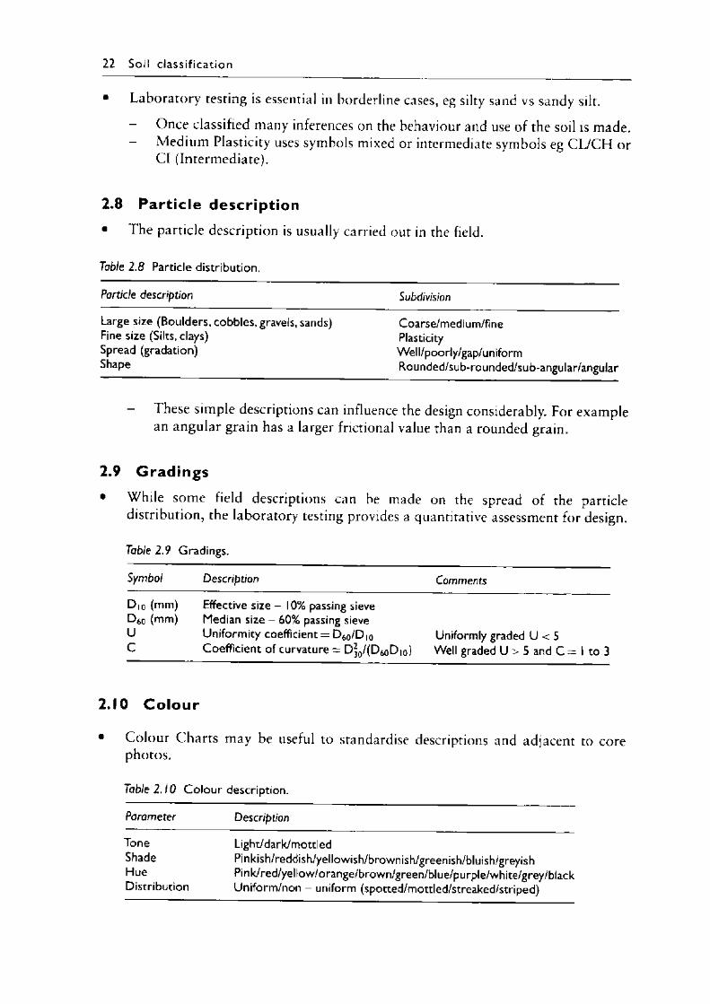
2.8 Part ic le descr iption• The particle description is usually carried out in the field.
Table 2.8 Particle distribution.
Particle description Subdivision
Large size (Boulders, cobbles, gravels, sands) Coarse/medium/fineFine size (Silts, clays) PlasticitySpread (gradation) Well/poorly/gap/uniformShape Rounded/sub-rounded/sub-angular/angular
- These simple descriptions can influence the design considerably. For example an angular grain has a larger frictional value than a rounded grain.
2.9 Gradings• While some field descriptions can be made on the spread of the particle
distribution, the laboratory testing provides a quantitative assessment for design.
Table 2.9 Gradings.
Symbol Description Comments
D |0 (mm) Effective size - 10% passing sieveD 60 (mm) Median size - 60% passing sieveU Uniformity coefficient = D 60/D,0 Uniformly graded U < 5C Coefficient of curvature = D 30/(D60D |0) Well graded U > 5 and C = 1 to 3
2.10 C o lo u r
• Colour Charts may be useful to standardise descriptions and adjacent to core photos.
Table 2.10 Co lour description.
Parameter Description
Tone Light/dark/mottledShade Pinkish/reddish/yellowish/brownish/greenish/bluish/greyishHue Pink/red/yellow/orange/brown/green/blue/purple/white/grey/blackDistribution Uniform/non - uniform (spotted/mottled/streaked/striped)
So il c la s s i f ic a t io n 23
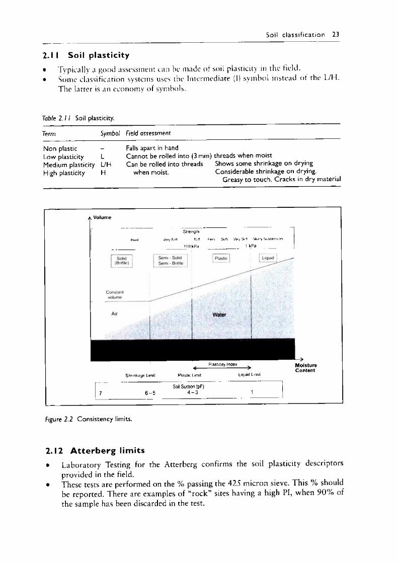
2 .1 I Soil plasticity• Typically a good assessment can he made of soil plasticity in the field.• Some classification systems uses the Intermediate (I) symbol instead of the I./H.
The latter is an economy of symbols.
Table 2 . 11 Soil plasticity.
Term Symbol Field assessment
Non plastic -Low plasticity LMedium plasticity L/H High plasticity H
Falls apart in handCannot be rolled into (3 mm) threads when moist Can be rolled into threads Shows some shrinkage on drying
when moist. Considerable shrinkage on drying.Greasy to touch. Cracks in dry material
Volum e
StrengthVery Sliff Stiff Firm Soft Very Soft Slurry Su spen sio n
110 kPa 1 kPa
Plasticity Index M oistureCo ntent
Shrinkage Limit Plastic Limit Liquid Limit
Soil Suction (pF)7 6 - 5 4 - 3 1
Figure 2.2 Consistency limits.
2.12 A tte rb e rg limits• Laboratory Testing for the Atterberg confirms the soil plasticity descriptors
provided in the field.• These tests are performed on the % passing the 4 2 5 micron sieve. This % should
be reported. There are examples of “ rock” sites having a high PI, when 9 0 % of the sample has been discarded in the test.
24 Soil c la ss i f ica t ion
Table 2.12 Atterberg limits.
Symbol Description Comments
LL Liquid limit - minimum moisture content at which a soil will flow under its own weight.
C on e penetrometer test or casagrande apparatus.
PL Plastic limit - Minimum moisture content at which a 3 mm thread of soil can be rolled with the hand without breaking up.
Test
SL Shrinkage limit - Maximum moisture content at which a further decrease of moisture content does not cause a decrease in volume of the soils.
Test.
PI Plasticity Index = LL-PL Derived from other tests.LS Linear shrinkage is the minimum moisture content for
soil to be mouldable.Test. Used where difficult
to establish PL and LL. PI = 2.13 LS.
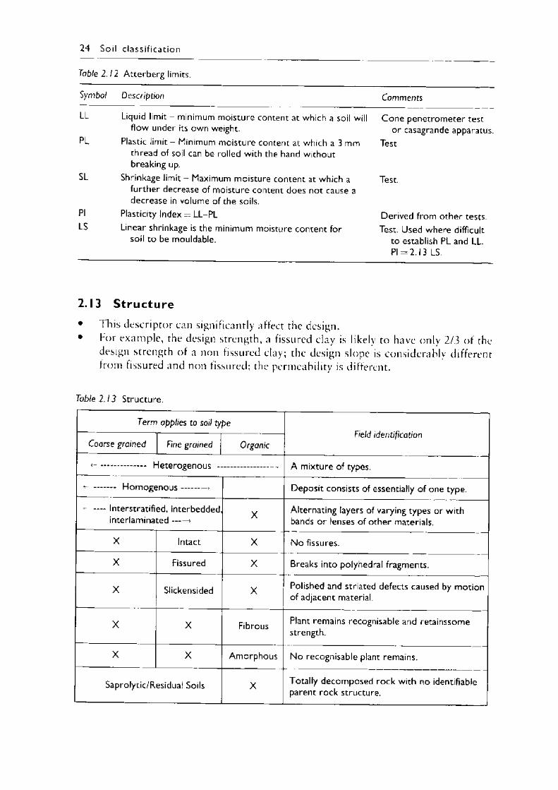
2.13 S tructure• I his descriptor can significantly affect the design.• For example, the design strength, a fissured clay is likely to have only 2/3 of the
design strength of a non fissured clay; the design slope is considerably different from fissured and non fissured; the permeability is different.
Table 2.13 Structure.
Term applies to soil typeField identification
Coarse grained Fine grained Organic
<—.................... Heterogenous ....................... —> A mixture of types.
.......... Homogenous........ —► Deposit consists of essentially of one type.
*------ Interstratified, interbeddedinterlaminated-----» X Alternating layers of varying types or with
bands or lenses of other materials.
X Intact X No fissures.
X Fissured X Breaks into polyhedral fragments.
X Slickensided X Polished and striated defects caused by motion of adjacent material.
X X Fibrous Plant remains recognisable and retainssome strength.
X X Amorphous No recognisable plant remains.
Saprolytic/Residual Soils X Totally decomposed rock with no identifiable parent rock structure.
Soil c la ss i f ica t io n 25
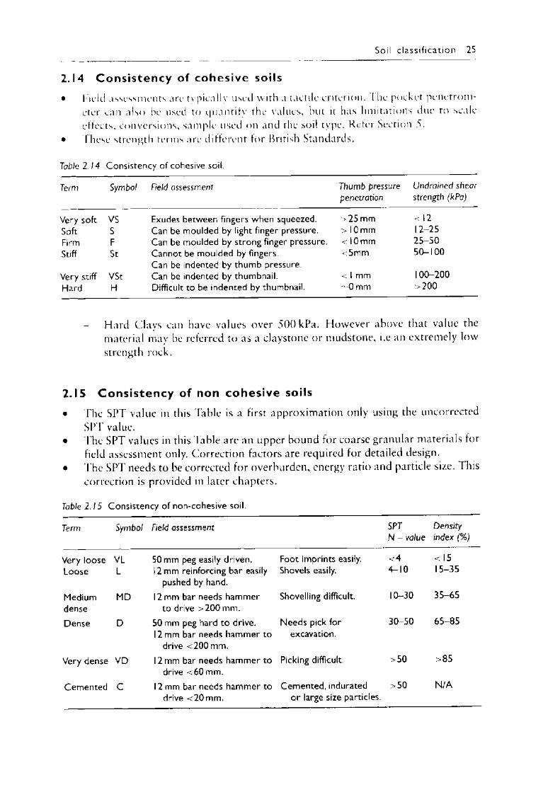
2.14 C o n s i s t e n c y of cohes ive soils• Held assessments are tvpicallv used with a tactile criterion. I he pocket penetrom
eter can also he used to quantify the values, but it has limitations due to scale effects, conversions, sample used on and the soil type. Refer Section 5.
• These strength terms arc different tor British Standards.
Table 2 .14 Consistency of cohesive soil.
Term Symbol Field assessment Thumb pressure Undrained shearpenetration strength (kPa)
Very soft VS Exudes between fingers when squeezed. >25 mm <12Soft S Can be moulded by light finger pressure. > 10 mm 12-25Firm F Can be moulded by strong finger pressure. < 10 mm 25-50Stiff St Cannot be moulded by fingers. <5 mm 50-100
Can be indented by thumb pressureVery stiff VSt Can be indented by thumbnail. < 1 mm 100-200Hard H Difficult to be indented by thumbnail. ~0 mm >200
— Hard Clays can have values over 500 kPa. However above that value the material may be referred to as a claystone or mudstone, i.e an extremely low strength rock.
2.15 C ons istency of non cohesive soils• The SPT value in this Table is a first approximation only using the uncorrected
SPT value.• The SPT values in this Table are an upper bound for coarse granular materials for
field assessment only. Correction factors are required for detailed design.• The SPT needs to be corrected for overburden, energy ratio and particle size. This
correction is provided in later chapters.
Table 2.15 Consistency of non-cohesive soil.
Term Symbol Field assessment SPTN - value
Density index (%)
Very loose VL 50 mm peg easily driven. Foot imprints easily. <4 <15Loose L 12 mm reinforcing bar easily
pushed by hand.Shovels easily. 4-10 15-35
Mediumdense
MD 12 mm bar needs hammer to drive >200 mm.
Shovelling difficult. 10-30 35-65
Dense D 50 mm peg hard to drive.12 mm bar needs hammer to
drive <200 mm.
Needs pick for 30-50 excavation.
65-85
Very dense VD 12 mm bar needs hammer to drive < 6 0 mm.
Picking difficult. >50 >85
Cemented C 12 mm bar needs hammer to drive <20 mm.
Cemented, indurated >50 or large size particles.
N/A
26 Soil c la ss i f ic a t ion
- Cemented is shown in the Table, as an extension to what is shown in most references.
- N - Values > 5 0 often considered as rock.Table applies to medium grain size sand. Material finer or coarser may have a different value. Correction factors also need to be applied. Refer Tables 5.4 and 5.5.
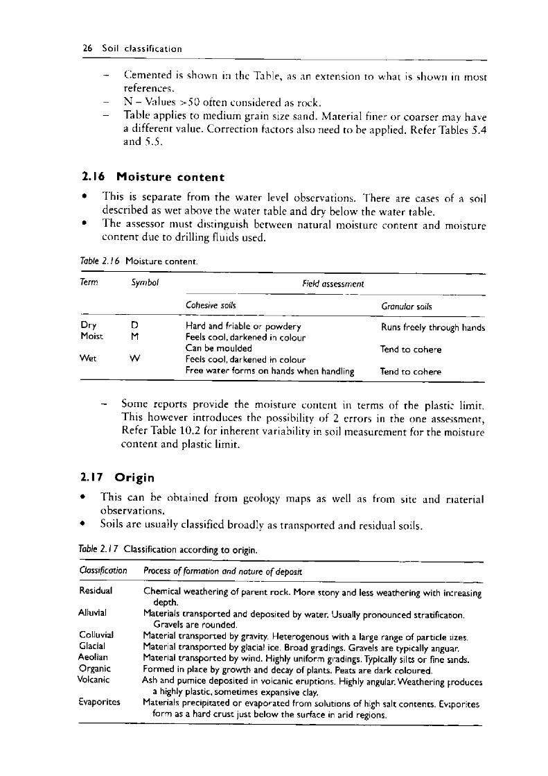
2.16 Moisture content• This is separate from the water level observations. There are cases of a soil
described as wet above the water table and dry below' the water table.• The assessor must distinguish between natural moisture content and moisture
content due to drilling fluids used.
Table 2.16 Moisture content.
Term Symbol Field assessment
Cohesive soils Granular soils
Dry D Hard and friable or powdery Runs freely through handsMoist M Feels cool, darkened in colour
Can be moulded Tend to cohereWet W Feels cool, darkened in colour
Free water forms on hands when handling Tend to cohere
Some reports provide the moisture content in terms of the plastic limit. This however introduces the possibility of 2 errors in the one assessment, Refer Table 10.2 for inherent variability in soil measurement for the moisture content and plastic limit.
2.17 Orig in• This can be obtained from geology maps as well as from site and material
observations.• Soils are usually classified broadly as transported and residual soils.
Table 2 . 1 7 Classification according to origin.
Classification Process o f formation and nature o f deposit
Residual
Alluvial
ColluvialGlacialAeolianOrganicVolcanic
Evaporites
Chemical weathering of parent rock. More stony and less weathering with increasing depth.
Materials transported and deposited by water. Usually pronounced stratification. Gravels are rounded.
Material transported by gravity. Heterogenous with a large range of particle sizes.Material transported by glacial ice. Broad gradings. Gravels are typically anguar.Material transported by wind. Highly uniform gradings. Typically silts or fine smds.Formed in place by growth and decay of plants. Peats are dark coloured.Ash and pumice deposited in volcanic eruptions. Highly angular. Weathering produces
a highly plastic, sometimes expansive clay.Materials precipitated or evaporated from solutions of high salt contents. Eviporites
form as a hard crust just below the surface in arid regions.
Soil c la s s i f ic a t io n 27
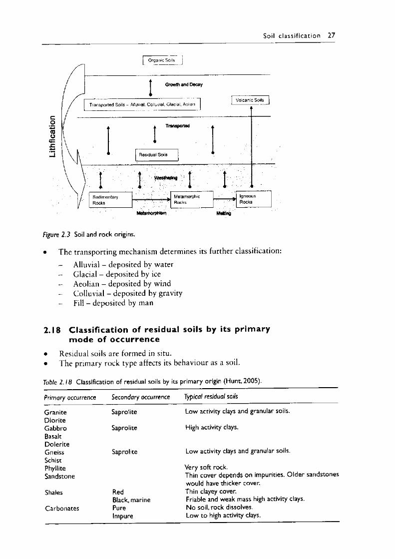
Figure 2.3 Soil and rock origins.
• The transporting mechanism determines its further classification:
Alluvial - deposited by water- Glacial - deposited by ice- Aeolian - deposited by wind
Colluvial - deposited by gravity Fill - deposited by man
2.18 Classif ication of residual soils by its pr im ary mode of occurrence
• Residual soils are formed in situ.• The primary rock type affects its behaviour as a soil.
Table 2.18 Classification of residual soils by its primary origin (Hunt, 2005).
Primary occurrence Secondary occurrence Typical residual soils
Granite Saprolite Low activity clays and granular soils.DioriteGabbro Saprolite High activity clays.BasaltDoleriteGneiss Saprolite Low activity clays and granular soils.SchistPhyllite Very soft rock.Sandstone Thin cover depends on impurities. O lder sandstones
would have thicker cover.Shales Red Thin clayey cover.
Black, marine Friable and weak mass high activity clays.Carbonates Pure No soil, rock dissolves.
Impure Low to high activity clays.
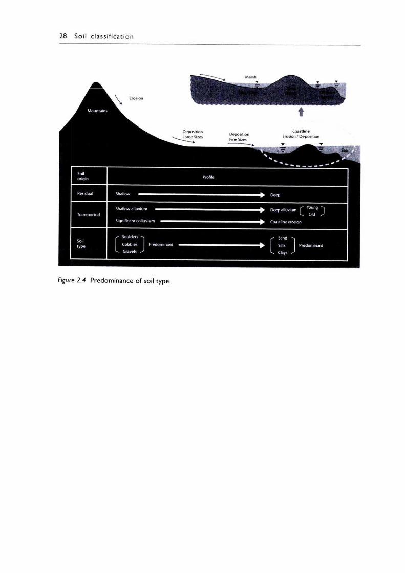
Coastline Erosion / Deposition
Figure 2.4 Predominance of soil type.
Ch apter 3
Rock classification
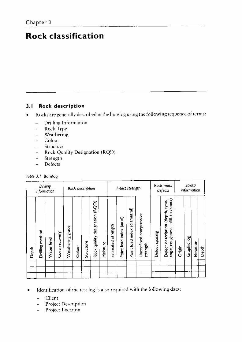
3.1 Rock description• Rocks are generally described in the borelog using the following sequence of terms:
- Drilling Information- Rock Type- Weathering- Colour- Structure
Rock Quality Designation (RQD)- Strength
Defects
Table 3 .1 Borelog.
Drillinginformation
Rock description Intact strength Rock mass defects
Stratainformatio n
Dept
h
Drilli
ng
met
hod
Wat
er l
evel
Core
re
cove
ry
Wea
ther
ing
grad
e
Colo
ur
Stru
ctur
e
Rock
qu
ality
desig
natio
n (R
QD
)
Moi
stur
e
Estim
ated
str
engt
h
Point
load
ind
ex
(axia
l)-
Point
load
ind
ex
(diam
etra
l)
Unco
nfin
ed
com
pres
sive
stren
gth
Defe
ct sp
acin
g
Defe
ct de
scrip
tion
(dep
th,
type
, an
gle,
roug
hnes
s, inf
ill, t
hick
ness
)
Orig
in
Grap
hic
logEle
vatio
nDe
pth
• Identification of the test log is also required with the following data:
Client- Project Description
Project Location
30 R o c k c lass i f ica t ion
- Project Number- Sheet N o . ___ o f ____
Reference: Easting, Northing, Elevation, Inclination- Date started and completed
3.2 Field rock core log• The field core log may be different from the final report log. Refer previous notes
(Section 2.2) on field log versus final log.• The field log variation is based on the strength tests not being completed at the
time of boxing the cores.• Due to the relatively slow rate of obtaining samples (as compared to soil) then
there would be time to make some assessments. However, some supervisors preferto log all samples in the laboratory, as there is a benefit in observing the full core length at one session.
- For example, the rock quality designation (RQD). If individual box cores are used, the assessment is on the core run length. If all boxes for a particular borehole are logged simultaneously, the assessment R Q D is on the domain length (preferable).
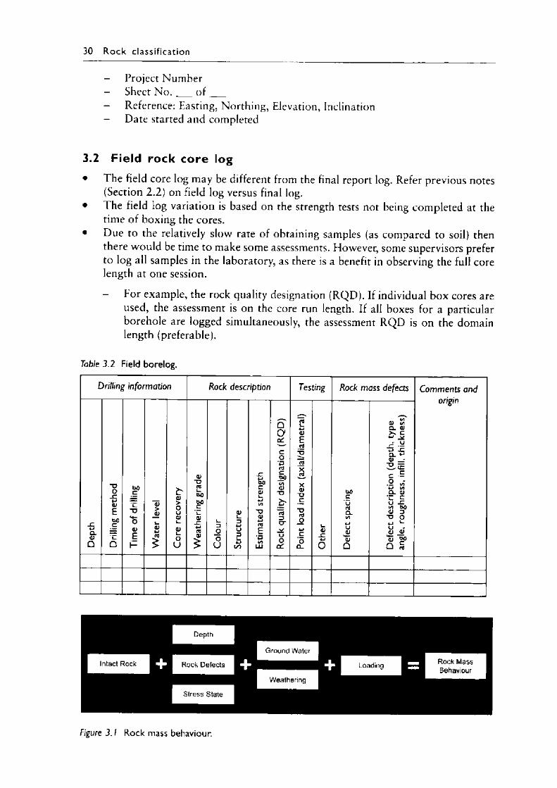
Table 3.2 Field borelog.
Drilling information Rock description Testing Rock mass defects Comments and origin
Dept
h
Drilli
ng
met
hod
Time
of dr
illing
Wat
er l
evel
Core
re
cove
ry
Wea
ther
ing
grad
e
Colo
ur
Stru
ctur
e
Estim
ated
str
engt
h
Rock
qu
ality
desig
natio
n (R
QD
)
Point
load
ind
ex
(axia
l/diam
etra
l)
Oth
er
Defe
ct sp
acin
g
Defe
ct de
scrip
tion
(dep
th,
type
an
gle,
roug
hnes
s, inf
ill, t
hick
ness
)
Depth
Ground Water9 Intact Rock E J j Rock Defects F S Loading ^ Mass 1Behaviour H
Stress StateWeathering
Figure 3 .1 Rock mass behaviour.
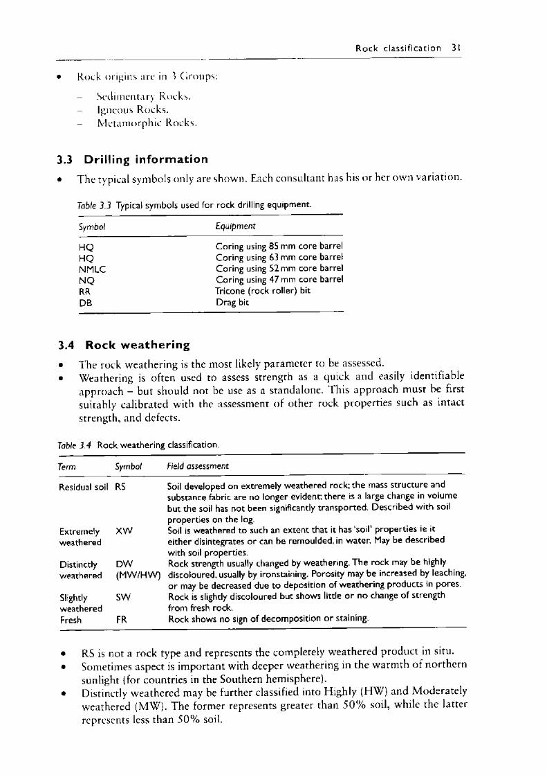
R o c k c la s s i f ic a t io n 31
• Rock origins are in 3 Groups:
Sedimentary Rocks.- Igneous Rocks.- Metamorphic Rocks.
3.3 Drill ing information• The typical symbols only are shown. Each consultant has his or her own variation.
Table 3.3 Typical symbols used for rock drilling equipment.
Symbol Equipment
H Q Coring using 85 mm core barrelH Q Coring using 63 mm core barrelNM LC Coring using 52 mm core barrelN Q Coring using 47 mm core barrelRR Tricone (rock roller) bitDB Drag bit
3.4 Rock weathering• The rock weathering is the most likely parameter to be assessed.• Weathering is often used to assess strength as a quick and easily identifiable
approach - but should not be use as a standalone. This approach must be first suitably calibrated with the assessment of other rock properties such as intact strength, and defects.
Table 3.4 Rock weathering classification.
Term Symbol
Residual soil RS
Extremelyweathered
Distinctlyweathered
SlightlyweatheredFresh
Field assessment
X W
D W(MW/HW)
SW
FR
Soil developed on extremely weathered rock; the mass structure and substance fabric are no longer evident; there is a large change in volume but the soil has not been significantly transported. Described with soil properties on the log.Soil is weathered to such an extent that it has ‘soil’ properties ie it either disintegrates or can be remoulded, in water. May be described with soil properties.Rock strength usually changed by weathering. The rock may be highly discoloured, usually by ironstaining. Porosity may be increased by leaching, or may be decreased due to deposition of weathering products in pores. Rock is slightly discoloured but shows little or no change of strength from fresh rock.Rock shows no sign of decomposition or staining.
• RS is not a rock type and represents the completely weathered product in situ.• Sometimes aspect is important with deeper weathering in the warmth of northern
sunlight (for countries in the Southern hemisphere).• Distinctly weathered may be further classified into Highly (HW) and Moderately
weathered (MW). The former represents greater than 5 0 % soil, while the latter represents less than 5 0 % soil.
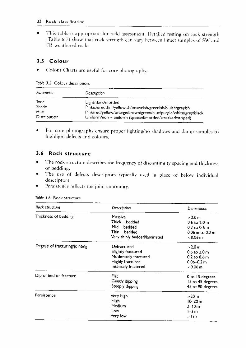
32 R o c k c lass i f ica t ion
• I his table is appropriate for field assessment. Detailed testing on rock strength (Table 6.7) show that rock strength can vary between intact samples of SW and FR weathered rock.
3.5 C o lo u r• Colour (.harts are useful for core photography.
Table 3.5 Colour description.
Parameter Description
Tone Light/dark/mottledShade Pinkish/reddish/yellowish/brownish/greenish/bluish/greyishHue Pink/red/yellow/orange/brown/green/blue/purple/white/grey/blackDistribution Uniform/non - uniform (spotted/mottled/streaked/striped)
• For core photographs ensure proper lighting/no shadows and damp samples to highlight defects and colours.
3.6 Rock structure• The rock structure describes the frequency of discontinuity spacing and thickness
of bedding.• The use of defects descriptors typically used in place of below individual
descriptors.• Persistence reflects the joint continuity.
Table 3.6 Rock structure.
Rock structure Description Dimensions
Thickness of bedding MassiveThick - bedded Mid - bedded Thin - beddedVery thinly bedded/laminated
>2.0 m 0.6 to 2.0 m 0.2 to 0.6 m 0.06 m to 0.2 m <0.06 m
Degree of fracturing/jointing Unfractured >2.0 mSlightly fractured 0.6 to 2.0 mModerately fractured 0.2 to 0.6 mHighly fractured 0.06-0.2 mIntensely fractured <0.06 m
Dip of bed or fracture Flat 0 to 15 degreesGently dipping 15 to 45 degreesSteeply dipping 45 to 90 degrees
Persistence Very high >20 mHigh 10-20 mMedium 3-10 mLow 1-3 mVery low >1 m
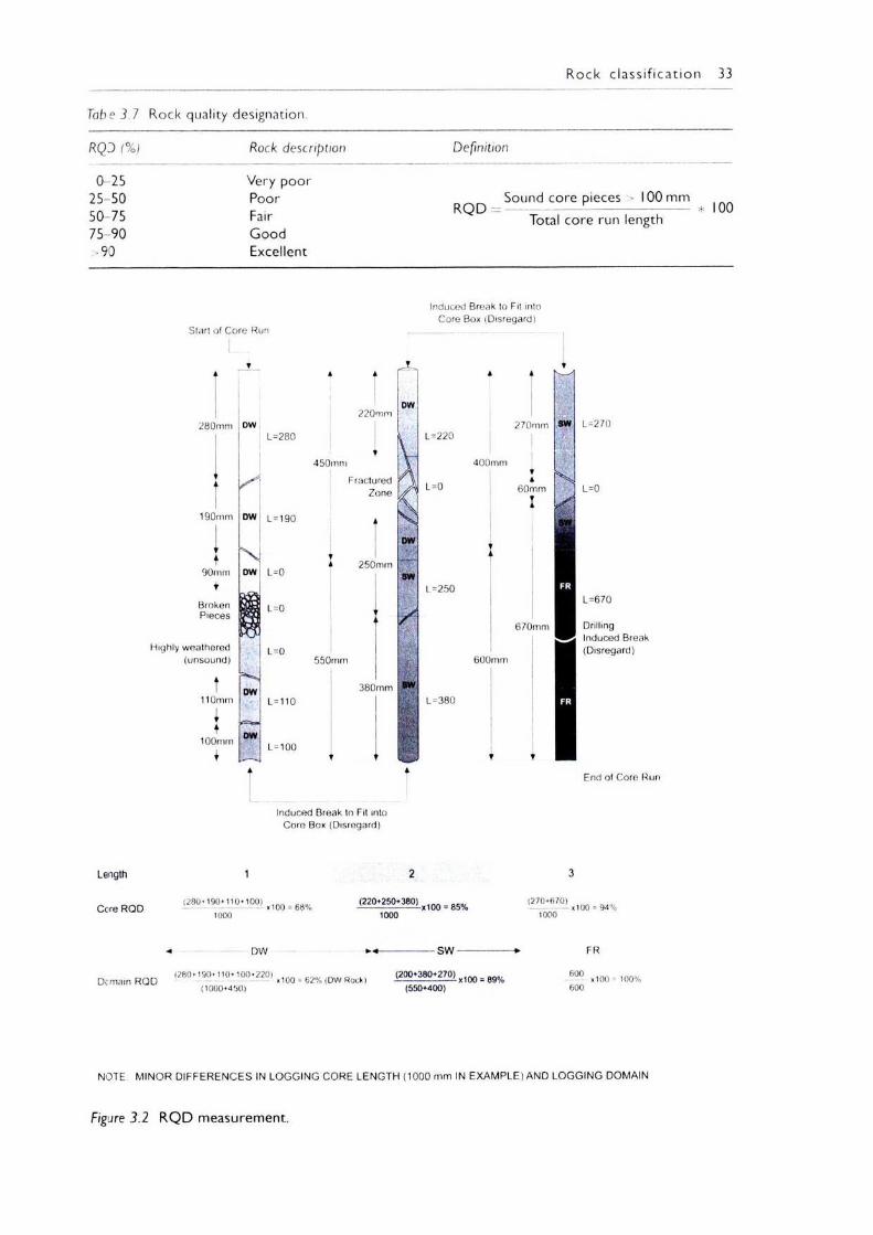
R o ck c la ss i f ica t io n 33
Tabe 3 .7 Rock quality designation.
RQD (%) Rock description Definition
0-2525-5050-7575-90>90
Very poorPoorFairGoodExcellent
Sound core piecesR Q D = - - -
Total core run> 100 mm
* 100length
Induced B reak to Fit into Core Box (D isregard)
Start of C o re Run
280mm DW
190mmI
t90mm
iBrokenPieces
Highly weathered (unsound)
t110mm
it
100mmI
L=280
DW |_=190
NDW | L=0
L=0
L=0
DW
DW
L= 110
L-1 0 0
220mmDW
450mmFractured
Zone
250mm
L-2 2 0
L=0
L=250
550mm
380mmL-3 8 0
400mm
270mm
»A60mm
sw 1=270
L=0
600mm
L=670
670mm DrillingInduced Break (D isregard)
End of Core Run
Induced Break to Fit into Core Box (Disregard)
Length 1 2 3
Cere ROD <280^ 110-1001 >100 = 68% (220*2M .360)t100 = 85% <270.670, ^ __ ^1000 1000 1000
DW ----------------SW ----------------- ► FR
D cm am R Q D Kl00 = 62% (DW Rock, <-2P-9 >3^ 2-™> ,100 = 89% “ L , 100 = 1001(1000+450) (550+400) 600
NOTE MINOR DIFFERENCES IN LOGGING CORE LENGTH (1000 mm IN EXAMPLE) AND LOGGING DOMAIN
Figure 3.2 R Q D measurement.
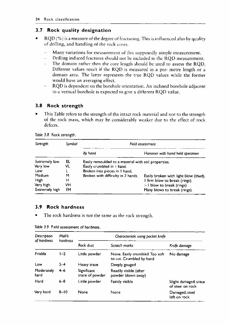
34 R o ck c lass i f ica t ion
3.7 Rock quality designation• R Q D (%) is a measure of the degree of fracturing. This is influenced also by quality
of drilling, and handling of the rock cores.
- Many variations for measurement of this supposedly simple measurement.- Drilling induced fractures should not be included in the R Q D measurement.- The domain rather then the core length should be used to assess the R Q D .
Different values result if the R Q D is measured in a per- metre length or adomain area. The latter represents the true R Q D values while the formerwould have an averaging effect.
- R Q D is dependent on the borehole orientation. An inclined borehole adjacent to a vertical borehole is expected to give a different R Q D value.
3.8 Rock strength• This Table refers to the strength of the intact rock material and not to the strength
of the rock mass, which may be considerably weaker due to the effect of rock defects.
Table 3.8 Rock strength.
Strength Symbol Field assessment
8/ hand Hammer with hand held specimen
Extremely low EL Easily remoulded to a material with soil properties.Very low VL Easily crumbled in 1 hand.Low L Broken into pieces in 1 hand.Medium M Broken with difficulty in 2 hands. Easily broken with light blow (thud).High H 1 firm blow to break (rings).Very high VH > 1 blow to break (rings)Extremely high EH Many blows to break (rings).
3.9 Rock hardness• The rock hardness is not the same as the rock strength.
Table 3.9 Field assessment of hardness.
Description Moll’s Characteristic using pocket knifeo f hardness hardness ---------------- — ----------------------------------------------
Rock dust Scratch marks Knife damage
Friable 1-2 Little powder None. Easily crumbled. Too soft to cut. Crumbled by hand
No damage
Low 2-4 Heavy trace Deeply gougedModeratelyhard
4-6 Significant trace of powder
Readily visible (after powder blown away)
Hard 6-8 Little powder Faintly visible Slight damaged; trace of steel on rock
Very hard 8-10 None None Damaged; steel left on rock
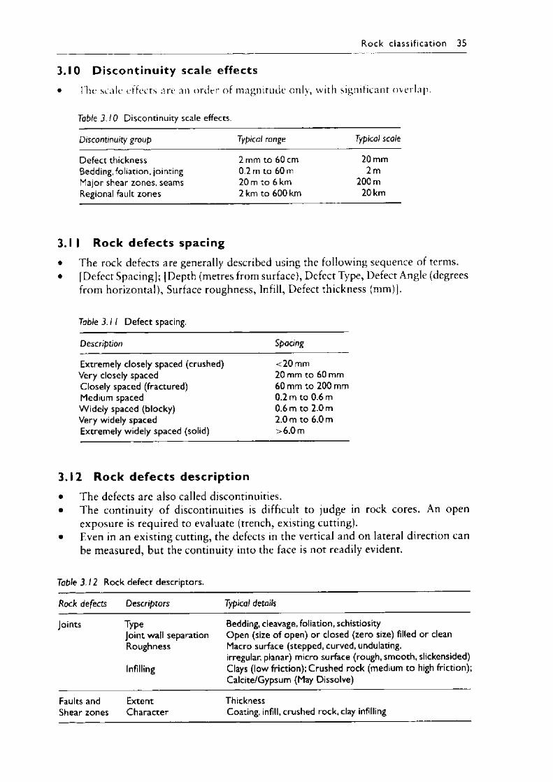
R o ck c lass i f ica t ion 35
3.10 D iscontinuity scale effects• The scale effects are an order of magnitude only, with significant overlap.
Table 3.10 Discontinuity scale effects.
Discontinuity group Typical range Typical scale
Defect thickness 2 mm to 60 cm 20 mmBedding, foliation, jointing 0.2 m to 60 m 2 mMajor shear zones, seams 20 m to 6 km 200 mRegional fault zones 2 km to 600 km 20 km
3.1 I Rock defects spacing• The rock defects are generally described using the following sequence of terms.• [Defect Spacing]; [Depth (metres from surface), Defect Type, Defect Angle (degrees
from horizontal), Surface roughness, Infill, Defect thickness (mm)].
Table 3 .11 Defect spacing.
Description Spacing
Extremely closely spaced (crushed) <20 mmVery closely spaced 20 mm to 60 mmClosely spaced (fractured) 60 mm to 200 mmMedium spaced 0.2 m to 0.6 mWidely spaced (blocky) 0.6 m to 2.0 mVery widely spaced 2.0 m to 6.0 mExtremely widely spaced (solid) >6.0 m
3.12 Rock defects description• The defects are also called discontinuities.• The continuity of discontinuities is difficult to judge in rock cores. An open
exposure is required to evaluate (trench, existing cutting).• Even in an existing cutting, the defects in the vertical and on lateral direction can
be measured, but the continuity into the face is not readily evident.
Table 3.12 Rock defect descriptors.
Rock defects Descriptors Typical details
Joints Type Bedding, cleavage, foliation, schistiosityJoint wall separation Open (size of open) or closed (zero size) filled or clean Roughness Macro surface (stepped, curved, undulating.
irregular, planar) micro surface (rough, smooth, slickensided) Infilling Clays (low friction); Crushed rock (medium to high friction);
Calcite/Gypsum (May Dissolve)
Faults and ExtentShear zones Character
ThicknessCoating, infill, crushed rock, clay infilling
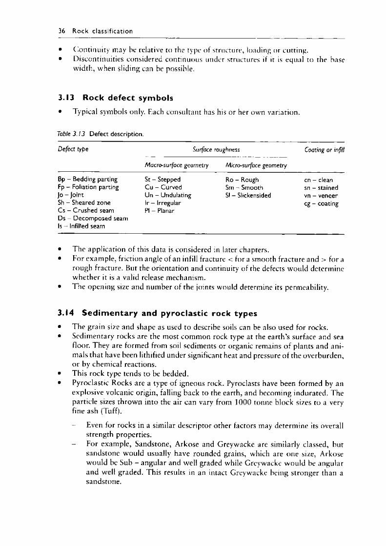
36 R o c k c la ss i f ica t ion
• Continuity may be relative to the type of structure, loading or cutting.• Discontinuities considered continuous under structures if it is equal to the base
width, when sliding can be possible.
3.13 Rock defect symbols• Typical symbols only. Each consultant has his or her own variation.
Table 3 .13 Defect description.
Defect type Surface roughness Coating or infill
Macro-surface geometry Micro-surface geometry
Bp - Bedding parting Fp - Foliation parting Jo - Joint Sh - Sheared zone Cs - Crushed seam Ds - Decomposed seam Is - Infilled seam
St - Stepped Cu - Curved Un - Undulating Ir - Irregular PI - Planar
Ro - Rough Sm - Smooth SI - Slickensided
cn - clean sn - stained vn - veneer eg - coating
• The application of this data is considered in later chapters.• For example, friction angle of an infill fracture < for a smooth fracture and > for a
rough fracture. But the orientation and continuity of the defects would determine whether it is a valid release mechanism.
• The opening size and number of the joints would determine its permeability.
3.14 S ed im entary and pyroclast ic rock types• The grain size and shape as used to describe soils can be also used for rocks.• Sedimentary rocks arc the most common rock type at the earths surface and sea
floor. They are formed from soil sediments or organic remains o f plants and animals that have been lithified under significant heat and pressure o f the overburden, or by chemical reactions.
• This rock type tends to be bedded.• Pyroclastic Rocks are a type of igneous rock. Pyroclasts have been formed by an
explosive volcanic origin, falling back to the earth, and becoming indurated. The particle sizes thrown into the air can vary from 1000 tonne block sizes to a very fine ash (Tuff).
- Even for rocks in a similar descriptor other factors may determine its overall strength properties.
- For example, Sandstone, Arkose and Greywacke are similarly classed, but sandstone would usually have rounded grains, which are one size, Arkose would be Sub - angular and well graded while Greywacke would be angular and well graded. This results in an intact Greywacke being stronger than a sandstone.
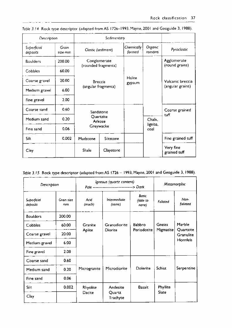
R o ck c la s s i f ic a t io n 37
Table 3 .14 Rock type descriptor* (adapted from AS 17 2 6 -1993, Mayne, 2001 and Geoguide 3, 1988).
Description Sedimentary
Superficialdeposits
Crain size mm Clastic (sediment) Chemically
formedOrganicremains Pyroclastic
Boulders 200.00 Conglomerate (rounded fragments)
Breccia (angular fragments)
Halitegypsum
Agglomerate (round grains)
Volcanic breccia (angular grains)
Cobbles 60.00
Coarse gravel 20.00
Medium gravel 6.00
Fine gravel 2.00
Coarse sand 0.60 SandstoneQuartzite
ArkoseGreywacke
Coarse grained tuff
Medium sand 0.20 Chalk,lignite,coalFine sand 0.06
Silt 0.002 Mudstone Siltstone Fine grained tuff
Clay Shale Claystone Very fine grained tuff
Table 3.15 Rock type descriptor (adapted from AS 1726 - 1993, Mayne, 2001 and Geoguide 3, 1988).
DescriptionIgneous (quartz content)
P a le ........................................... > DarkMetamorphic
Superficialdeposits
Crain size mm
Acid(much)
Intermediate(some)
Basic (little to none)
Foliated Nonfoliated
Boulders 200.00
Cobbles 60.00 GraniteAplite
GranodioriteDiorite
BabbroPeriodotite
GneissMigmatite
MarbleQuartziteGranuliteCoarse gravel 20.00
Medium gravel 6.00Hornfels
Fine gravel 2.00
Coarse sand 0.60
Medium sand 0.20 Microgranite Microdiorite Dolerite Schist Serpentine
Fine sand 0.06
Silt 0.002 RhyoliteDacite
Andesite Quartz T rachyte
Basalt PhylliteSlate
Clay
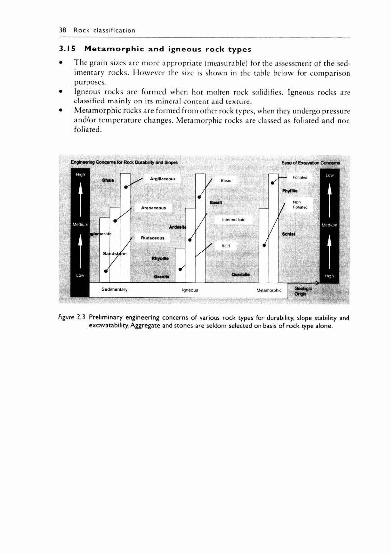
38 R o c k c la s s i f ic a t io n
3.15 M etam orph ic and igneous rock types• The grain sizes are more appropriate (measurable) for the assessment of the sed
imentary rocks. However the size is shown in the table below for comparison purposes.
• Igneous rocks are formed when hot molten rock solidifies. Igneous rocks are classified mainly on its mineral content and texture.
• Metamorphic rocks are formed from other rock types, when they undergo pressure and/or temperature changes. Metamorphic rocks are classed as foliated and non foliated.
Engineering Concerns for Rock Durability and Slopes
Shale
S a n d sldsjm
Argillaceous
Arenaceous
Amfeslfc i
t Rudaceous
RhyoIHe
Granite✓
J
// Basic
Basalt
Intermediate
✓
J
Ease of Excavation Concerns
— Foliated
Phyllits
/NonFoliated
Schist
Sedim entary Igneous Metamorphic GeologicOrigin
Figure 3.3 Preliminary engineering concerns of various rock types for durability, slope stability and excavatability. Aggregate and stones are seldom selected on basis of rock type alone.
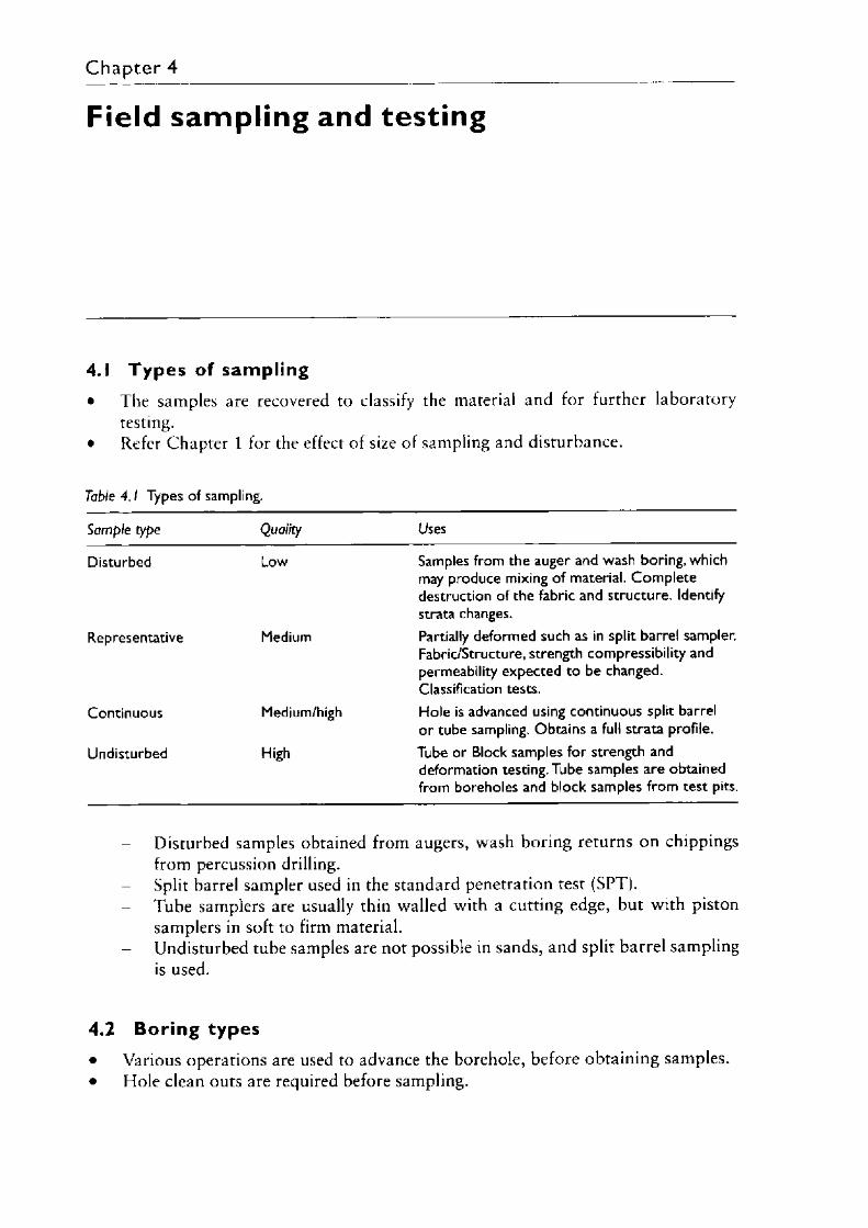
C h a p te r 4
Field sampling and testing
4.1 T ypes of sampling• The samples are recovered to classify the material and for further laboratory
testing.• Refer Chapter 1 for the effect of size of sampling and disturbance.
Table 4 .1 Types of sampling.
Sample type Quality Uses
Disturbed Low Samples from the auger and wash boring, which may produce mixing of material. Complete destruction of the fabric and structure. Identify strata changes.
Representative Medium Partially deformed such as in split barrel sampler. Fabric/Structure, strength compressibility and permeability expected to be changed. Classification tests.
Continuous Medium/high Hole is advanced using continuous split barrel or tube sampling. Obtains a full strata profile.
Undisturbed High Tube or Block samples for strength and deformation testing. Tube samples are obtained from boreholes and block samples from test pits.
- Disturbed samples obtained from augers, wash boring returns on chippings from percussion drilling.
- Split barrel sampler used in the standard penetration test (SPT).- Tube samplers are usually thin walled with a cutting edge, but with piston
samplers in soft to firm material.- Undisturbed tube samples are not possible in sands, and split barrel sampling
is used.
4.2 Boring types• Various operations are used to advance the borehole, before obtaining samples.• Hole clean outs are required before sampling.
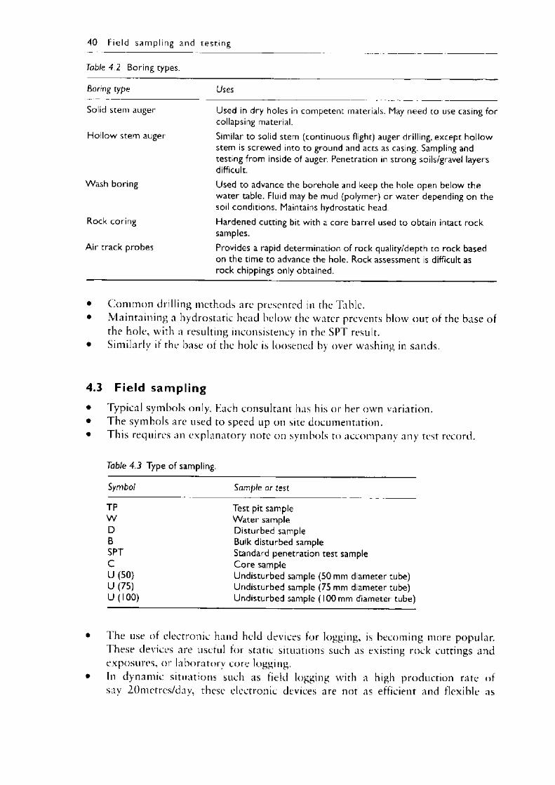
40 F ie ld sampling and testing
Table 4.2 Boring types.
Boring type Uses
Solid stem auger Used in dry holes in competent materials. May need to use casing forcollapsing material.
Hollow stem auger Similar to solid stem (continuous flight) auger drilling, except hollowstem is screwed into to ground and acts as casing. Sampling andtesting from inside of auger. Penetration in strong soils/gravel layersdifficult.
Wash boring Used to advance the borehole and keep the hole open below thewater table. Fluid may be mud (polymer) or water depending on thesoil conditions. Maintains hydrostatic head.
Rock coring Hardened cutting bit with a core barrel used to obtain intact rocksamples.
Air track probes Provides a rapid determination of rock quality/depth to rock basedon the time to advance the hole. Rock assessment is difficult asrock chippings only obtained.
• Com mon drilling methods are presented in the Table.• Maintaining a hydrostatic head below the water prevents blow out of the base of
the hole, with a resulting inconsistency in the SPT result.• Similarly if the base of the hole is loosened by over washing in sands.
4.3 Field sampling• Typical symbols only. Each consultant has his or her own variation.• The symbols are used to speed up on site documentation.• This requires an explanatory note on symbols to accompany any test record.
Table 4.3 Type of sampling.
Symbol Sample or test
TP Test pit sampleW Water sampleD Disturbed sampleB Bulk disturbed sampleSPT Standard penetration test sampleC Core sampleU (50) Undisturbed sample (50 mm diameter tube)U (75) Undisturbed sample (75 mm diameter tube)U (100) Undisturbed sample (100 mm diameter tube)
The use of electronic hand held devices for logging, is becoming more popular. These devices are useful for static situations such as existing rock cuttings and exposures, or laboratory core logging.In dynamic situations such as field logging with a high production rate of say 20metres/day, these electronic devices are not as efficient and flexible as
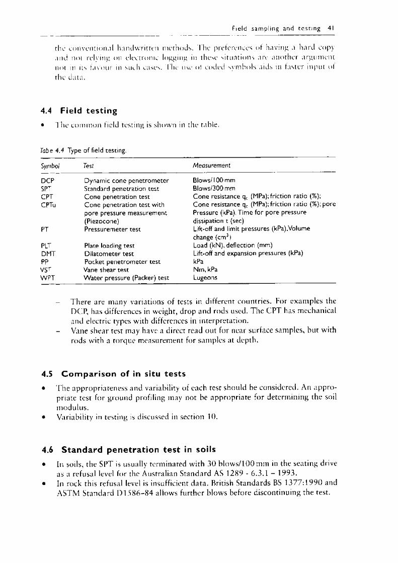
Field sampling and tes t in g 41
the conventional handwritten methods. I he preferences of having a hard copy and not relying on electronic logging in these situations are another argument not in its favour in such cases. 1 he use of coded symbols aids in faster input of the data.
4.4 Field testing• T he common field testing is shown in the table.
Tabe 4.4 Type of field testing.
Symbol Test Measurement
DCP Dynamic cone penetrometer Blows/100 mmSPT Standard penetration test Blows/300 mmCPT Cone penetration test Cone resistance qc (MPa); friction ratio (%);CPTu Cone penetration test with Cone resistance qc (MPa); friction ratio (%); pore
pore pressure measurement Pressure (kPa).Time for pore pressure(Piezocone) dissipation t (sec)
PT Pressuremeter test Lift-off and limit pressures (kPa),Volumechange (cm3)
PLT Plate loading test Load (kN), deflection (mm)DMT Dilatometer test Lift-off and expansion pressures (kPa)PP Pocket penetrometer test kPaVST Vane shear test Nm, kPaW PT W ater pressure (Packer) test Lugeons
- There are many variations of tests in different countries. For examples the DCP, has differences in weight, drop and rods used. The CPT has mechanical and electric types with differences in interpretation.Vane shear test may have a direct read out for near surface samples, but with rods with a torque measurement for samples at depth.
4.5 C o m p a r iso n of in situ tests• T he appropriateness and variability of each test should be considered. An appro
priate test for ground profiling may not be appropriate for determining the soil modulus.
• Variability in testing is discussed in section 10.
4.6 Standard penetration test in soils• In soils, the SPT is usually terminated with 3 0 blows/100 mm in the seating drive
as a refusal level for the Australian Standard AS 1289 - 6.3.1 - 1993.• In rock this refusal level is insufficient data. British Standards BS 1 3 7 7 :1 9 9 0 and
ASTM Standard D 1 5 8 6 - 8 4 allows further blows before discontinuing the test.
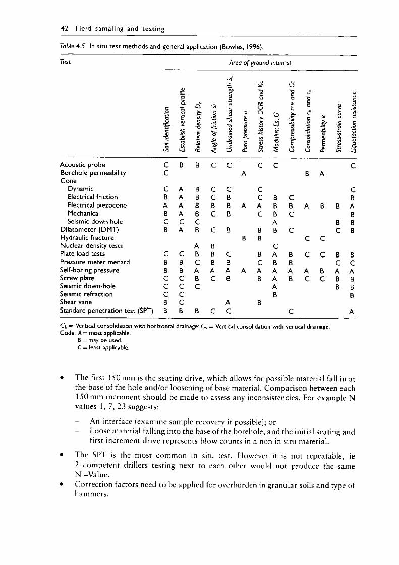
42 F ie ld sampling and test ing
Table 4.5 In situ test methods and general application (Bowles, 1996).
Test Area o f ground interest
c<u
ooo
2-Cl
-oo♦-JiS3
Q.£•00Ca;
<uQC
Otxoc
-ctxoc
~oajc'§c
3<L)3co00
8J■CL
oTDCoa:uObo♦-j-Coo00QJ
o00*
U J
.3*oo
Cj~oco>E
00£■CL£Oo
uco
co♦3OooocoO
-QOai§
co8<vc r
Acoustic probe C B B C C C C CBorehole permeability C A B ACone
Dynamic C A B C C C CElectrical friction B A B C B C B C BElectrical piezocone A A B B B A A B B A B B AMechanical B A B C B C B C BSeismic down hole C C C A B B
Dilatometer (DMT) B A B C B B B C C BHydraulic fracture B B C CNuclear density tests A B CPlate load tests C C B B C B A B C C B BPressure meter menard B B C B B C B B C CSelf-boring pressure B B A A A A A A A A B A AScrew plate C C B C B B A B C C B BSeismic down-hole C C C A B BSeismic refraction C C B BShear vane B C A BStandard penetration test (SPT) B B B C C C A
Q, = Vertical consolidation with horizontal drainage: C v = Vertical consolidation with vertical drainage. Code: A = most applicable.
8 = may be used.C = least applicable.
• The first 150 mm is the seating drive, which allows for possible material fall in at the base of the hole and/or loosening of base material. Comparison between each 150 mm increment should be made to assess any inconsistencies. For example N values 1, 7, 23 suggests:
- An interface (examine sample recovery if possible); orLoose material falling into the base of the borehole, and the initial seating and first increment drive represents blow counts in a non in situ material.
• The SPT is the most common in situ test. However it is not repeatable, ie 2 competent drillers testing next to each other would not produce the same N -Value.
• Correction factors need to be applied for overburden in granular soils and type of hammers.
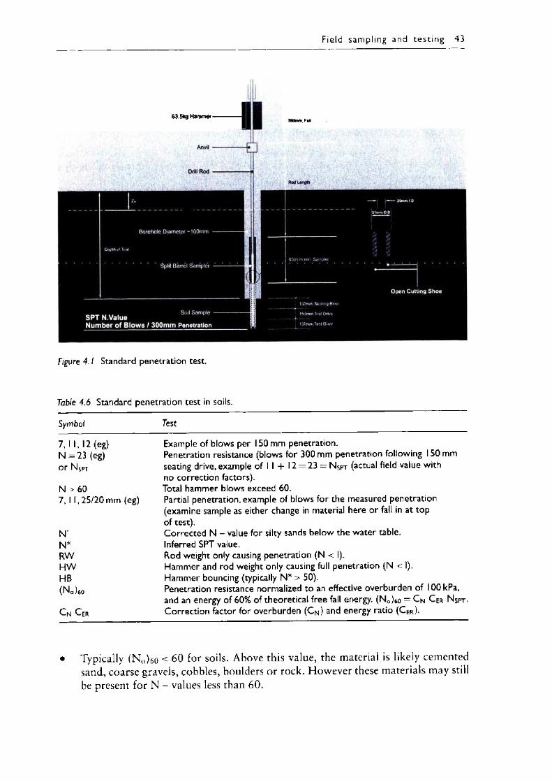
F ie ld sampling and test ing 43
Borehole Diameter -100mm
Split Barrel Sampler
S P T N .ValueN u m b e r of B lo w s / 300m m Penetration
□ p e n C u t t in g S h o e
63.5kg Hammer
Anvil
Drill Rod
760mm Fall
Rod Length
150mm Seating Blow
150mm Tesl Drivo
150mm Test Oiive
Oepift o i Teal
Figure 4 .1 Standard penetration test.
Table 4.6 Standard penetration test in soils.
Symbol Test
7, I 1, 12 (eg) Example of blows per 150 mm penetration.N = 23 (eg) Penetration resistance (blows for 300 mm penetration following 150 mmor N Spt seating drive, example of I I + 12 = 23 = N s p t (actual field value with
no correction factors).N > 60 Total hammer blows exceed 60.7, I 1, 25/20 mm (eg) Partial penetration, example of blows for the measured penetration
(examine sample as either change in material here or fall in at top of test).
N Corrected N - value for silty sands below the water table.N* Inferred SPT value.RW Rod weight only causing penetration (N < I).HW Hammer and rod weight only causing full penetration (N < I).HB Hammer bouncing (typically N* > 50).
Z 0 o Penetration resistance normalized to an effective overburden of lOOkPa,and an energy of 60% of theoretical free fall energy. (N0)6o = C N C Er N Sp t-
C n C er Correction factor for overburden (C N) and energy ratio (C Er ).
• Typically (N())6o < 60 for soils. Above this value, the material is likely cemented sand, coarse gravels, cobbles, boulders or rock. However these materials may still be present for N - values less than 60.
44 F ie ld sampling and testing
• While the SPT N - value is the summation of the 300 mm rest drive, the incremental change should also be noted, as this may signify loose fall in of material (ie incorrect values) or change in strength (or layer) profile over that 4 5 0 mm.
4.7 Standard penetration test in rock• The SPT procedure in rock is similar to that in soils but extending the refusal
blows to refusal. This requires at least 30 blows in less than 100 mm, for both a seating and a test drive before discontinuing the test.
• Tabulate both the seating and the test drive. The driller may complain about damage to the equipment.
• A solid cone (apex angle of 60°) is used for tests in gravelly soils, boulders and soft weathered rock.
• Values o f N > 60 that cannot be extrapolated to a value of 120 or above is of very little quantitative value to the designer or assessing rock strength.
Table 4.7 Standard penetration test in rock.
Symbol Test
N = 23 (eg) Penetration resistance (blows for 300 mm penetration following 150 mm seatingdrive, example of II -h 12 = 23).
— 30/50 mm, Partial penetration, example of blows for the measured penetration, but allowing30/20 mm (eg) for measuring both seating and test drive.N* Inferred SPT Value.
• There is a debate on whether inferred values should be placed on a factual log.However, the debate then extends to how much on the log is factual. For example,is the colour description (person dependent) more factual than N * .
4.8 O verb urd en correct ion factors to SPT result• An overburden correction factor applies for granular materials.• n „ = C n N.
Table 4.8 SPT correction factors to account for overburden pressure (adapted from Skempton, 1986).
Effeaiveoverburden(kPa)
Correction factor, CN
Approximate depth o f soil (metres) to achieve nominated effective overburden pressure for various ground water level (zw)
Finesands
Coarsesands
At surface zw = 0 m
zw = 2 m zw = 5 m z w= 10m
0 2.0 1.5 0.0 m 0.0 m 0.0 m 0.0 m25 1.6 1.3 3.1 m 1.4 m 1.4m 1.4 m50 1.3 1.2 6.2 m 3.7 m 2.8 m 2.8 m
100 1.0 1.0 12.5 m 10.0 m 6.2 m 5.6 m200 0.7 0.8 25.0 m 22.5 m 18.8 m 12.5 m300 0.5 0.6 37.5 m 35.0 m 31.2m 25.0 m400 0.5 0.5 50.0 m 47.5 m 43.7m 37.5 m
• Average saturated unit weight of 18kN/irT used in Table. Unit weight canva ry.
• Borehole water balance is required for tests below the water table to avoid blow out at the base of the hole with loosening of the soil, and a resulting non representative low N - value.
• In very fine or silty sands below the water table, a pore pressure may develop and an additional correction factor applies for N' > 15. N = 15 + I/2 (N' — 15).
4.9 Equ ipm ent and borehole correction factors for SPT result• An equipment correction and borehole size correction factors apply.• The effect of borehole diameter is negligible for cohesive soils, and no correction
factor is required.• The energy ratio is normalized to 6 0 % of total energy.• (N())m) = Cn Chr N.• Q . ; r = C | | C r C s C b .
Table 4.9 Energy ratio correction factors to be applied to SPT value to account for equipment andborehole size (adapted from Skempton, 1986 andTakimatsu and Seed, 1987).
To account for Parameter Correction factor
Field sampling and tes t in g 45
Hammer - release - country
Hammer (C H) • Donut - free fall (Tombi) - Japan 1.3• Donut - rope and pulley-Japan l.l• Safety - rope and pulley - USA 1.0• Donut - free fall (Trip) - Europe, 1.0
China, Australia• Donut - rope and pulley - China 0.8• Donut - rope and pulley - USA 0.75
Rod length (C R) • 10 m 1.0• 10 m to 6 m 0.95• 6 m to 4 m 0.85• 4 m to 3 m 0.75
Sampler (C s) • Standard 1.0• US sampler without liners 1.2
Borehole • 65 mm - 1 15 mm 1.0Diameter (C B) • 150 mm 1.05
• 200 mm 1.15
4.10 C one penetrat ion test• There are several variations of the cone penetration test (CPT). Electric and
mechanical cones should be interpreted differently.• The CPTu data is tabled below. The CPT would not have any of the pore pressure
measurements.• The CPT has a high production rate (typically 100 m/day but varies depending
on number, soil type, distance between tests, accessibility, etc) compared to other profile testing.
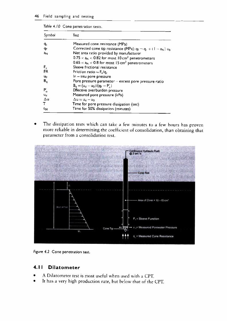
46 F ie ld sampling and testing
Table 4.10 Cone penetration tests.
Symbol Test
qc Measured cone resistance (MPa)9t Corrected cone tip resistance (MPa): qy = qc + (1 - aN) ubaN Net area ratio provided by manufacturer
0.75 < aN < 0.82 for most 10 cm2 penetrometers0.65 < aN < 0.8 for most 15 cm2 penetrometers
Fs Sleeve frictional resistanceFR Friction ratio = Fs/qcuo In - situ pore pressureBq Pore pressure parameter - excess pore pressure ratio
Bq — (ud - u 0)/(qr - PG)Po Effective overburden pressureUd Measured pore pressure (kPa)Au Au = ud - u0T Time for pore pressure dissipation (sec)t50 Time for 50% dissipation (minutes)
The dissipation tests which can take a few minutes to a few hours has proven more reliable in determining the coefficient of consolidation, than obtaining that parameter from a consolidation test.
Figure 4.2 Cone penetration test.
4.11 D i la t o m e t e r• A Dilatometer test is most useful when used with a CPT.• It has a very high production rate, but below that of the CPT.
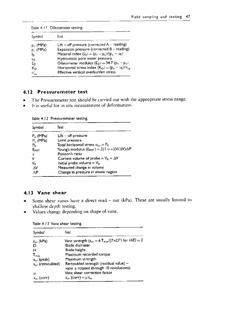
Fie ld sampling and tes t in g 47
Table 4 .1 I Dilatometer testing.
Symbol Test
pD (MPa) Lift - off pressure (corrected A - reading)pi (MPa) Expansion pressure (corrected B - reading)|D Material index (lD) = (pi - p0)/(po - uo)u0 Hydrostatic pore water pressureEd Dilatometer modulus (ED) = 34.7 (pt - pQ)K d Horizontal stress index (KD) = (pQ - uo)/a^Qo' Effective vertical overburden stress
V O
4.12 P r e s s u r e m e t e r test• The Pressuremeter test should be carried out with the appropriate stress range.• It is useful for in situ measurement of deformation.
Table 4 .12 Pressuremeter testing.
Symbol Test
P0 (MPa) Lift - off pressurePL (MPa) Limit pressureP0 Total horizontal stress aho = PoEpmt Youngs modulus (EPMt ) = 2(1 + v)(V/AV)APv Poisson’s ratioV Current volume of probe = V0 + AVV 0 Initial probe volume = V0AV Measured change in volumeA P Change in pressure in elastic region
4.13 V a n e s h e a r• Some shear vanes have a direct read - out (kPa). These are usually limited to
shallow depth testing.• Values change depending on shape of vane.
Table 4.13 Vane shear testing.
Symbol Test
sUv (kPa) Vane strength (suv = 6 T max/(77iD3) for H/D = 2D Blade diameterH Blade heightT max Maximum recorded torquesUv (peak) Maximum strengthsuv (remoulded) Remoulded strength (residual value) -
vane is rotated through 10 revolutions)M- Vane shear correction factorsuv (corr) suv (corr) = |isuv
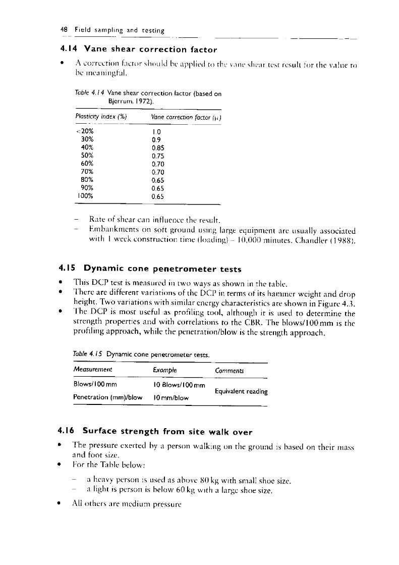
48 F ie ld sampling and testing
4.14 V a n e sh ea r c o r r e c t io n factor• A correction factor should be applied to the vane shear test result for the value to
be meaningful.
Table 4 .14 Vane shear correction factor (based on Bjerrum, 1972).
Plasticity index (%) Vane correction factor (n )
<20% 1.030% 0.940% 0.8550% 0.7560% 0.7070% 0.7080% 0.6590% 0.65
100% 0.65
- Rate of shear can influence the result.Embankments on soft ground using large equipment are usually associated with I week construction time (loading) - 10,000 minutes. Chandler (1988) .
4.15 D y n a m ic co ne p e n e t r o m e t e r tests• This DCP test is measured in two ways as shown in the table.• There are different variations of the DCP in terms of its hammer weight and drop
height. Two variations with similar energy characteristics are shown in Figure 4.3.• I he DCP is most useful as profiling tool, although it is used to determine the
strength properties and with correlations to the CBR. The blows/100 mm is theprofiling approach, while the penetration/blow is the strength approach.
Table 4.15 Dynamic cone penetrometer tests.
Measurement Example Comments
Blows/100 mm 10 Blows/100 mmEquivalent reading
Penetration (mm)/blow 10 mm/blow
4.16 S u r fa c e s t re n g th f rom site walk over• 1 he pressure exerted by a person walking on the ground is based on their mass
and foot size.• For the Table below:
- a heavy person is used as above 80 kg with small shoe size.- a light is person is below 60 kg with a large shoe size.
• All others are medium pressure
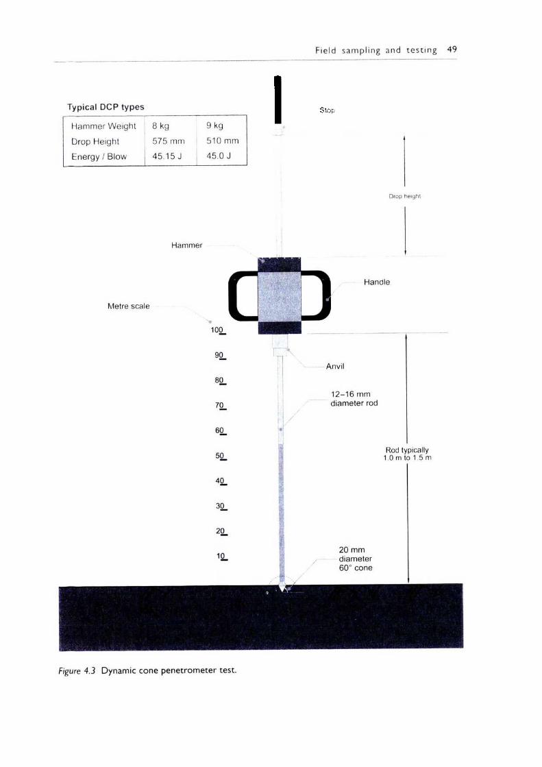
Field sampling and tes t in g 49
Typical DCP types
Hammer Weight 8 kg 9 kgDrop Height 575 mm 510 mmEnergy / Blow 45.15 J 45.0 J
Drop height
Metre scale
Hammer
100_
go.
80_
70-
60.
50_
40,
30.
20,
10
o \
Handle
Anvil
12-16 mmdiameter rod
Rod typically 1.0 m to 1.5 m
20 mm diameter 60° cone
Figure 4.3 Dynamic cone penetrometer test.
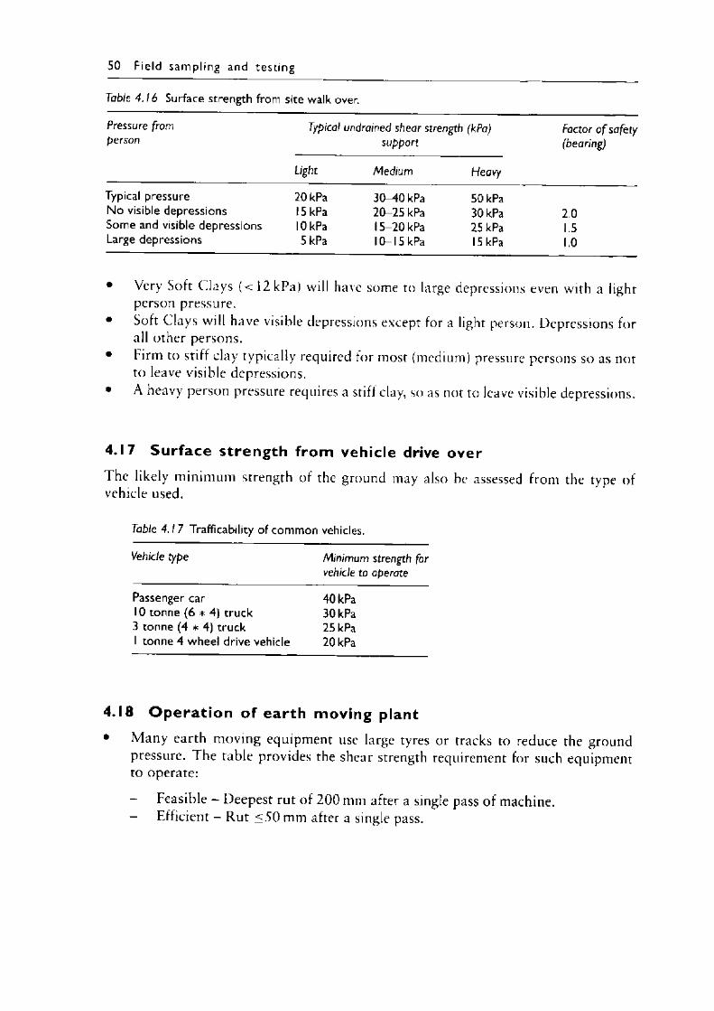
50 F ie ld sam pling and testing
Table 4.16 Surface strength from site walk over.
Pressure from Typical undrained shear strength (kPa) Factor o f safetyperson support (bearing)
Light Medium Heavy
Typical pressure 20 kPa 30-40 kPa 50 kPaNo visible depressions 15 kPa 20-25 kPa 30 kPa 2.0Some and visible depressions lOkPa 15-20 kPa 25 kPa 1.5Large depressions 5 kPa 10-15 kPa 15 kPa 1.0
• Very Soft Clays (< 12 kPa) will have some to large depressions even with a light person pressure.
• Soft Clays will have visible depressions except for a light person. Depressions for all other persons.
• Hrm to stiff clay typically required for most (medium) pressure persons so as not to leave visible depressions.
• A heavy person pressure requires a stiff clay, so as not to leave visible depressions.
4.17 S u r fa c e s t re n g th f rom vehic le drive overThe likely minimum strength of the ground may also be assessed from the type of vehicle used.
Table 4.1 7 Trafficability of common vehicles.
Vehicle type Minimum strength for vehicle to operate
Passenger car 40 kPa10 tonne (6 * 4) truck 30 kPa3 tonne (4 * 4) truck 25 kPa1 tonne 4 wheel drive vehicle 20 kPa
4.18 O p e r a t i o n of e a r th m oving plant• Many earth moving equipment use large tyres or tracks to reduce the ground
pressure. The table provides the shear strength requirement for such equipment to operate:
- Feasible - Deepest rut of 2 0 0 mm after a single pass of machine.- Efficient - Rut < 5 0 mm after a single pass.
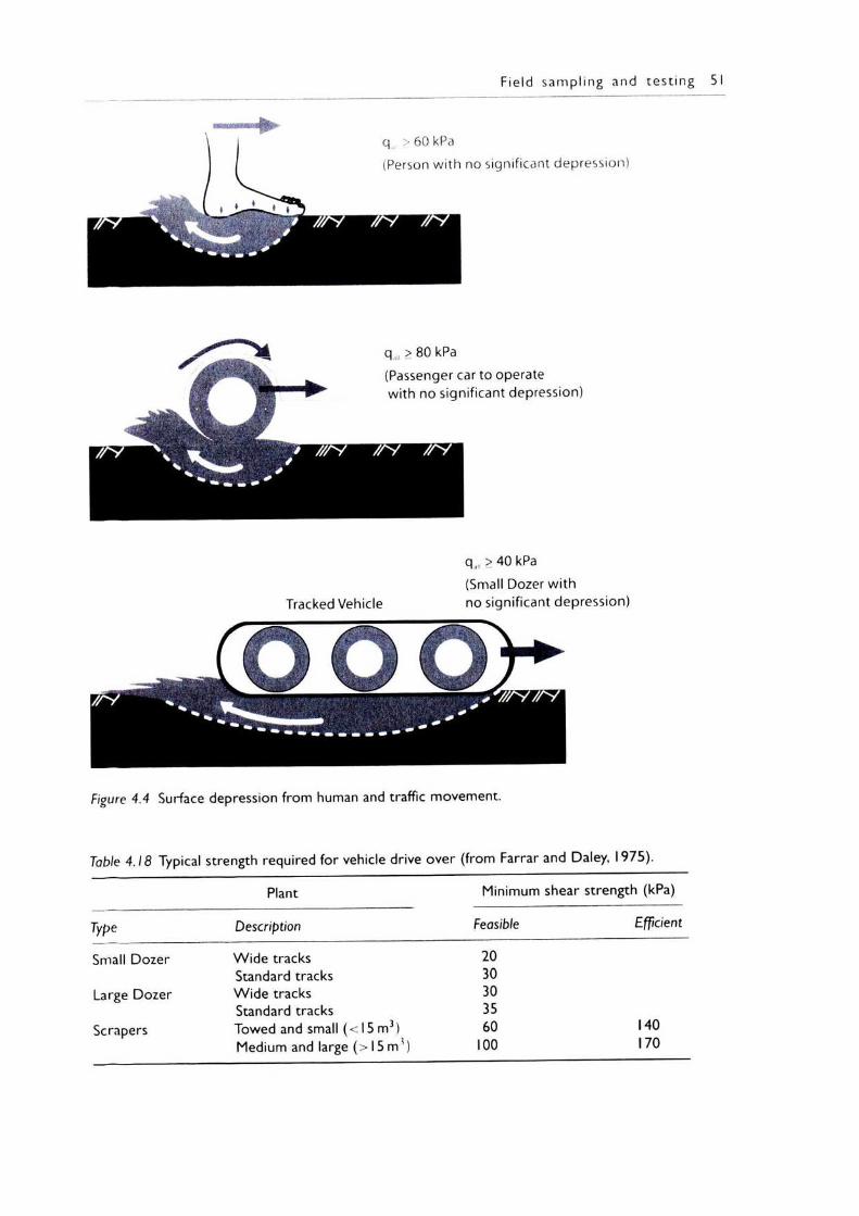
Field sam pling and tes t in g 51
no significant depression)
q il( > 80 kPa(Passenger car to operate with no significant depression)
qall > 40 kPa(Small Dozer with
Tracked Vehicle no significant depression)
Figure 4.4 Surface depression from human and traffic movement.
Table 4.18 Typical strength required for vehicle drive over (from Farrar and Daley, 1975).
Plant Minimum shear strength (kPa)
Type Description Feasible Efficient
Small Dozer
Large Dozer
Scrapers
W ide tracks 20Standard tracks 30W ide tracks 30Standard tracks 35Towed and small (< 15 m3) 60 140Medium and large (> 15 m *) 100 170

Chapter 5
Soil strength param eters from classification and testing
5.1 E r r o r s in m e a s u r e m e n t• The industry trend is to minimise laboratory testing in favour of correlations from
borelogs. This is driven by commercial incentives to reduce the investigation costs and win the project.
• This approach can often lead to conservative, but sometimes incorrect designs.
Table 5 .1 Errors in measurement.
Type o f error
Inherent soil variability Sampling error
Measurement error
Statistical variation
Comment
Sufficient number of tests can minimise this error.Correct size sample/type of sampler to account for soil structure and sensitivity in situ testing for granular material.Not all test results from even accredited laboratories should be used directly. Sufficient number of laboratory tests to show up "outliers”.Understand limitation of the tests.Validate with correlation tests.Appreciate significant variation correlations however.Use results knowing that results do vary (Chapter 10). Use of values appropriate to the risk and confidence of test results.
- Clay strength is typically 5 0 % to 1 0 0 % of value obtained from a 38 mm sample. Larger samples capture the soil structure effect (refer Table 1.13).
5.2 C la y s t re n g th from pocket p e n e t r o m e t e r• The pocket penetrometer (PP) is the simplest quantitative test used as an alternative
to the tactile classification of strength (Table 2.14) .• The approximation of PP value — 2 C L1 is commonly used. C u (kPa) = q u/2.
However this varies for the type of soil as shown in the table.
54 Soil s trength p a ram ete rs f ro m c lass i f ica t ion and testing
Some considerations in using this tool are:
- It does not consider scale effects- Caution on use of results when used in gravelly clays. This is not an
appropriate test in granular materials.- Do not use PP on an SPT sample, which are disturbed from the effects o f
driving (Table 4.1). Soft to firm samples are compressed and often provide stiff to very stiff results and hard samples are shattered and also provide stiff to very stiff results.
Table 5.2 Evaluating strength from PP values (Look, 2004).
Material Unconfined compressive strength qu
In general 0.8 PPFills 1.15 PPFissured clays 0.6 PP
• For Soils: Three Pocket Penetrometer (PP) Readings on Undisturbed tube sample (base of tube): Report the PP value - do not convert to a C\, on the borelog.
• Some field supervisors are known to use the PP on SPT samples - this practice is to be a voided as the PP value is meaningless on a disturbed sample.
5.3 C la y s t reng th from S P T data• As a first approximation C u = 5 SPT is commonly used. However this correlation
is known to vary from 2 to 8.• The overburden correction is not required for SPT values in clays.• Sensitivity of clay affects the results.
Table 5.3 Clay strength from SPT data.
Material Description SPT - N (blows/300 mm) Strength
Clay V. Soft <2 0-12 kPaSoft 2-5 12-25 kPaFirm 5-10 25-50 kPaStiff 10-20 50-100 kPaV Stiff 20-40 100-200 kPaHard >40 >200 kPa
• An indication of the variability of the correlation in the literature is as follows
Sower’s graphs uses C u = 4 N for high plasticity clays and increasing to about 15 N for low plasticity clays.
- Contrast with Stroud and Butler’s (1975) graph which shows Cu = 4.5 N forPI > 3 0 % , and increasing to Cu = 8 N for low plasticity clays (PI = 15%).
• 1 herefore use with caution, and with some local correlations.
Soil s t ren g th p a ra m e te rs f ro m c lass i f ica t ion and testing 55
5.4 C le a n sand strength f ro m S P T data• The values varv from corrected to uncorrected N values and type of sand.• T he SPT - value can he used to determine the degree of compactness of a cohesion-
less soil. However, it is the soil friction angle that is used as the strength parameter.
Table 5.4 Strength from SPT on clean medium size sands only.
Description Relative SPT - N (blows/300 mm) Strengthdensity D r -------------------------------------------------------
Uncorrected field value Corrected value Friction angle
V. Loose < 1 5% N < 4 (No)60< 3 4 x 2 8 °Loose 15-35% N = 4-10 (N0)6n = 3-8 4> = 28-30Med dense 35-65% N = 10-30 (N0)m» = 8-25 (|> = 30-40Dense 65-85% N = 3 0 -5 0 (N0U - 25-42 4> = 40-45V. Dense >85% N > 50 (N0)ft,i > 42 4) = 45°-50
100% (N0)6o = 60 <() = 50
• Reduce by 5° for clayey sand.• Increase <\> by 5° for gravely sand.
5.5 F ine and c o a r se sand s t re n g th f ro m S P T data• Fine sands have reduced values from the table above while coarse sand has an
increased strength value.• The corrected N value is used in the table below.
Table 5.5 Strength from corrected SPT value on clean fine and coarse size sands.
Description Relative Corrected SPT - N (blows/300 mm) Strengthdensity Dr ------------------------------------------------------ - '
Fine sand Medium Coarse sand
V. Loose < 15%
mVIJoz (N o)60 < 3 (No)60<3 cj) < 28
Loose 15-35% (No)60 = 3-7
00imIIovOoz
(N0 >60 = 3-8 cj) = 28-30Med dense 35-65% (N o)60 = 7-23 (N o>60 = 8-25 (No)60 = 8-27 4> = 30-40Dense 65-85% (N 0 )6o = 23—40 (N0 )60 = 25-43 (No)60 = 27—47 4> - 40—45V. Dense >85% ( N J 60> 40 (No)60> 43 (No)60 > 47 4> = 45-50
100% (No)60 — 55 (No)60 = 60 (No)60 = 65 4) = 50
• Above is based on Skempton (1988) :
(N())6o/Dr = 55 f ° r Fine Sands.(N„)60/D* = 60 for Medium Sands.
- (N()) 60/D“ = 65 for Coarse Sands.
5.6 Effect of aging• The SPT in recent fills and natural deposits should be interpreted differently.• Typically the usual correlations and interpretations are for natural materials. Fills
and remoulded samples should be assessed different.
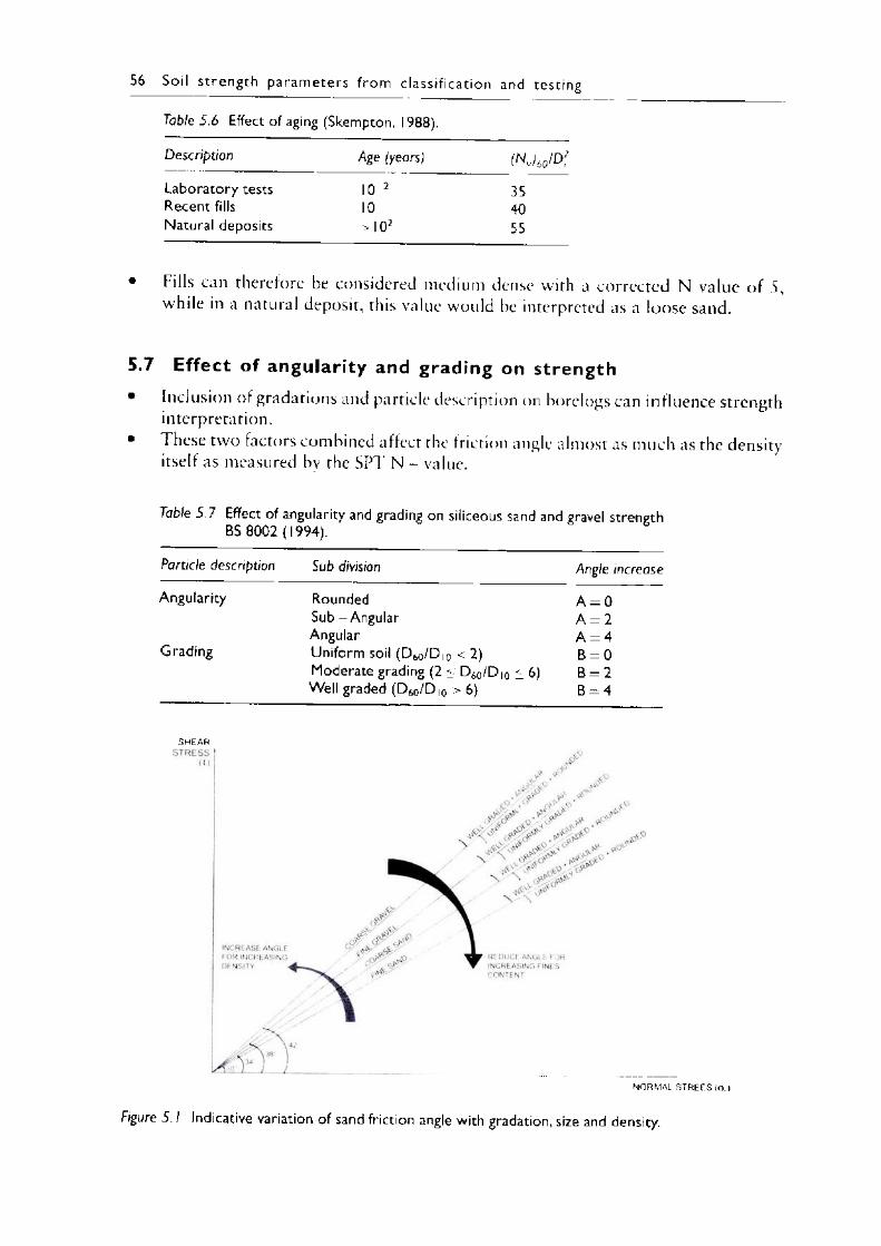
Soil strength param eters from classification and testin
Table 5.6 Effect of aging (Skeimpton, 1988).
Description Age (years) (N o ) J D 2r
Laboratory tests 10 2 35Recent fills 10 40Natural deposits > I0 2 55
• 1 ills can therefore he considered medium dense with a corrected N value o f 5, while in a natural deposit, this value would he interpreted as a loose sand.
5.7 Effect of angularity and grading on strength• Inclusion of gradations and particle description on borelogscan influence strength
interpretation.• These two factors combined affect the friction angle almost as much as the density
itself as measured by the SPT N - value.
Table 5 .7 Effect of angularity and grading on siliceous sand and gravel strength BS 8002 (1994).
Particle description Sub division Angle increase
Angularity Rounded A = 0Sub - Angular A = 2Angular A = 4
Grading Uniform soil (D 60/D|0 < 2) B = 0Moderate grading (2 < D 60/D|0 £ 6) B = 2Well graded (D 60/D,0 > 6) B = 4
SHEAR
NORMAL STREES (O.)
Figure 5 .1 Indicative variation of sand friction angle with gradation, size and density.
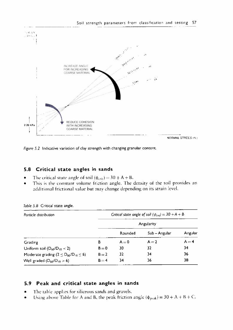
Soil s t reng th p a ram e te rs from c lass i f ica t ion and tes t in g 57
It AR
2-20 kPa
»NORMAL STREES (Cl
Figure 5.2 Indicative variation of clay strength with changing granular content.
5.8 Cr it ica l state angles in sandsThe critical state angle of soil (<t>Cr,t) = 30 + A + B.This is the constant volume friction angle. The density of the soil provides an additional frictional value but may change depending on its strain level.
Table 5.8 Critical state angle.
Particle distribution Critical state angle o f soil ((pcnt) — 30 + A + 8
Angularity
Rounded Sub-Angular Angular
Grading B A = 0 > II ro > II
Uniform soil (D 6o/D|0 < 2) B = 0 30 32 34Moderate grading (2 < D 60/D|0 5 6) B = 2 32 34 36Well graded (D 6q/D io > 6) B = 4 34 36 38
5.9 Peak and crit ical state angles in sands• The table applies for siliceous sands and gravels.• Using above Table for A and B, the peak friction angle (<t>ptak) = 30 + A + B + C.
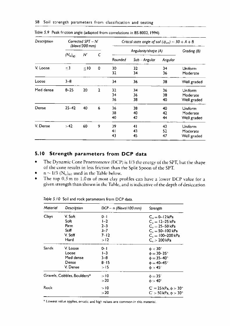
58 So il s t ren g th p a ra m e te rs f ro m c lass i f ica t io n and testing
Table 5 .9 Peak friction angle (adapted from correlations in BS 8002, 1994).
Description Corrected SPT - N' (blows/300 mm)
Critical state angle o f soil ((pcril) — 30 4- A + 8
Angularity/shape (A) Grading (B)(No)(,0 N ’ C
Rounded Sub - Angular Angular
V. Loose <3 <10 0 30 32 34 Uniform32 34 36 Moderate
Loose 3-8 34 36 38 Well graded
Med dense 8-25 20 2 32 34 36 Uniform34 36 38 Moderate36 38 40 Well graded
Dense 25-42 40 6 36 38 40 Uniform38 40 42 Moderate40 42 44 Well graded
V. Dense >42 60 9 39 41 43 Uniform41 43 52 Moderate43 45 47 Well graded
5.10 Strength param eters from D C P data• The Dynamic Cone Penetrometer (DCP) is 1/3 the energy of the SPT, but the shape
of the cone results in less friction than the Split Spoon of the SPT.• n ^ 1/3 (Nn)6o used in the Table below.• The top 0 .5 m to 1.0 m of most clay profiles can have a lower DCP value for a
given strength than shown in the Table, and is indicative of the depth of desiccation
Table 5 .10 Soil and rock parameters from D CP data.
Material Description DCP - n (Blows/100 mm) Strength
Clays V. Soft 0-1 C u = 0-12 kPaSoft 1-2 C u = 12-25 kPaFirm 2-3 C u = 25-50 kPaStiff 3-7 C u = 50-100 kPaV. Stiff 7-12 C u = 100-200 kPaHard >12 C u > 200 kPa
Sands V. Loose 0-1 4> < 30°Loose 1-3 <t> = 30-35Med dense 3-8 <|> = 35-40Dense 8-15 <|> = 40-45°V. Dense >15 cj) > 45°
Gravels, Cobbles, Boulders* >10 c1) = 35°>20 (j) > 40
Rock >10 C = 25 kPa, 4> > 30°>20 C' > 50 kPa, (j> > 30°
* Low est value applies, erratic and high values are common in this material.
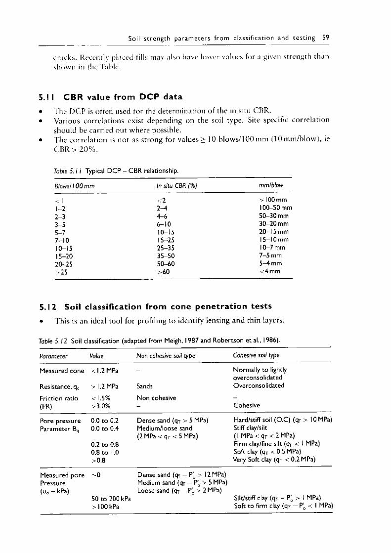
cracks. Recently placed tills may also have lower values for a given strength than shown 111 the l a Me.
Soil s t reng th p a ram e te rs f ro m c lass i f ica t ion and te s t in g 59
5.1 I C B R value from D C P data• The DCP is often used for the determination of the in situ CBR.• Various correlations exist depending on the soil type. Site specific correlation
should be carried out where possible.• The correlation is not as strong for values > 10 blows/100 mm (10 mm/blow), ie
C B R > 2 0 % .
Table 5 .11 Typical D CP - CB R relationship.
Blows/100 mm In situ CBR (%) mm/blow
<1 <2 > 100 mm1-2 2-4 100-50 mm2-3 4-6 50-30 mm3-5 6-10 30-20 mm5-7 10-15 20-15 mm7-10 15-25 15-10 mm10-15 25-35 10-7 mm15-20 35-50 7-5 mm20-25 50-60 5^4 mm>25 >60 <4 mm
5.12 Soil classif ication from cone penetrat ion tests• This is an ideal tool for profiling to identify lensing and thin layers.
Table 5.12 Soil classification (adapted from Meigh, 1987 and Robertson et al., 1986).
Parameter Value Non cohesive soil type Cohesive soil type
Measured cone
Resistance, qcFriction ratio (FR)
<1.2 MPa
>1.2 MPa< 1.5% >3.0%
SandsNon cohesive
Normally to lightlyoverconsolidatedOverconsolidated
Cohesive
Pore pressure Parameter Bq
0.0 to 0.2 0.0 to 0.4
0.2 to 0.8 0.8 to 1.0 >0.8
Dense sand (qT > 5 MPa) Medium/loose sand (2 MPa < qT < 5 MPa)
Hard/stiff soil (O .C) (qy > 10 MPa)Stiff clay/silt(1 MPa < qT < 2 MPa)Firm clay/fine silt (qr < 1 MPa)Soft clay (qr < 0.5 MPa)Very Soft clay (qy < 0.2 MPa)
Measured pore Pressure (ud - kPa)
- 0
50 to 200 kPa >100 kPa
Dense sand (qr — PQ > Medium sand (qr - P Loose sand (qr - PQ >
12 MPa) > 5 MPa) 2 MPa)
Silt/stiff clay (qj - Pq > 1 MPa)Soft to firm clay (qj - P'a < 1 MPa)
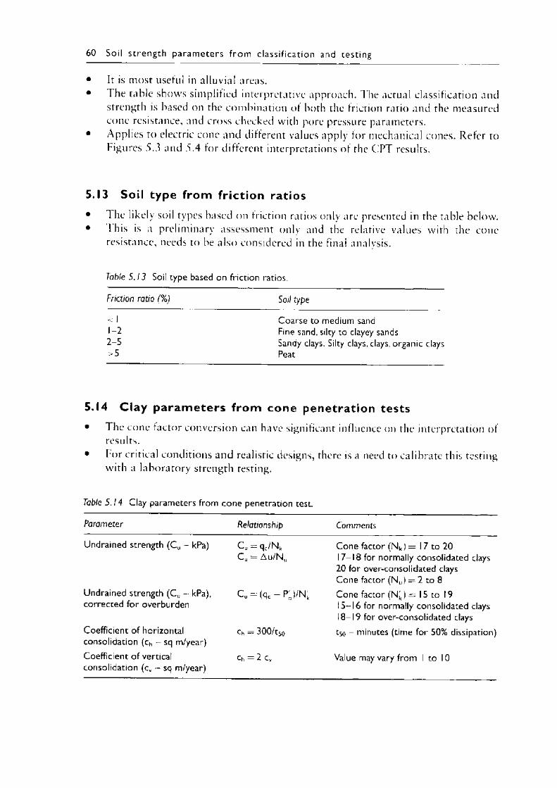
• It is most useful in alluvial areas.• The table shows simplified interpretative approach. The actual classification and
strength is based on the combination of both the friction ratio and the measured cone resistance, and cross checked with pore pressure parameters.
• Applies to electric cone and different values apply for mechanical cones. Refer to Figures 5.3 and 5.4 for different interpretations of the CPT results.
5.13 Soil type from fr iction ratios• 1 he likely soil types based on friction ratios only are presented in the table below.• I his is a preliminary assessment only and the relative values with the cone
resistance, needs to be also considered in the final analysis.
60 So il s t reng th p a ra m e te rs f ro m c lass i f ica t ion and testing
Table 5.13 Soil type based on friction ratios.
Friction ratio (%) Soil type
<1 Coarse to medium sand1-2 Fine sand, silty to clayey sands2-5 Sandy clays. Silty clays, clays, organic clays>5 Peat
5.14 C lay param eters from cone penetration tests• The cone factor conversion can have significant influence on the interpretation of
results.• For critical conditions and realistic designs, there is a need to calibrate this testing
with a laboratory strength testing.
Table 5. 1 4 Clay parameters from cone penetration test.
Parameter Relationship Comments
Undrained strength (C u - kPa) C u = q c/Nk C u = Au/Nu
Cone factor (Nk) = 17 to 20 17-18 for normally consolidated clays 20 for over-consolidated clays Cone factor (Nu) = 2 to 8
Undrained strength (C u - kPa), corrected for overburden
Cu = (qc - P ;) / N ' Cone factor (Nk) = 15 to 19 15-16 for normally consolidated clays 18-19 for over-consolidated clays
Coefficient of horizontal consolidation (ch - sq m/year)
ch — 300/t50 t50 - minutes (time for 50% dissipation)
Coefficient of vertical consolidation (cv - sq m/year)
Ch = 2 cv Value may vary from 1 to 10
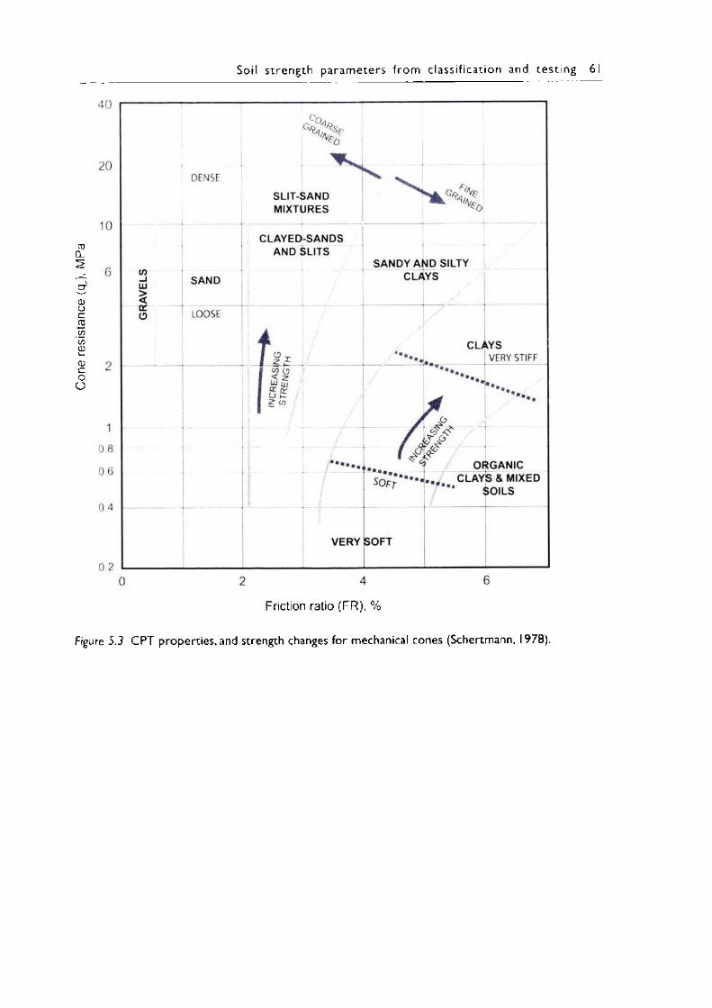
Cone
re
sista
nce
(qj,
MPa
Soil s t reng th p a ra m e te rs from c lass i f ica t io n and tes t in g 61
Friction ratio (F R ), %
Figure 5.3 C P T properties, and strength changes for mechanical cones (Schertmann, 1978).
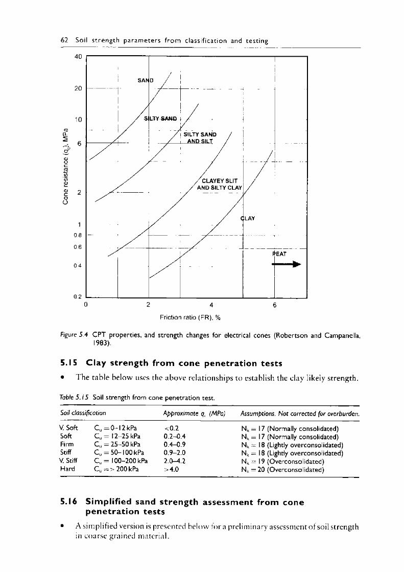
62 So il s t reng th p a ram ete rs f ro m c lass i f ica t ion and testing
Friction ratio (F R ), %
Figure 5.4 C P T properties, and strength changes for electrical cones (Robertson and Campanella, 1983).
5.15 C lay strength from cone penetration tests• The table below uses the above relationships to establish the clay likely strength.
Table 5.15 Soil strength from cone penetration test.
Soil classification Approximate qt (MPa) Assumptions. Not corrected for overburden.
V. Soft C u = 0 - l2 k P a <0.2 Nk — 17 (Normally consolidated)Soft C u = 12-25 kPa 0.2-0.4 Nk = 17 (Normally consolidated)Firm C u = 25-50 kPa 0.4-0.9 Nk = 18 (Lightly overconsolidated)Stiff C y = 50-100 kPa 0.9-2.0 Nk = 18 (Lightly overconsolidated)V. Stiff C u = 100-200 kPa 2.0—4.2 Nk = 19 (Overconsolidated)Hard C u = > 200 kPa >4.0 Nk = 20 (Overconsolidated)
5.16 Simplified sand strength assessment from cone penetrat ion tests
• A simplified version is presented below fora preliminary assessment of soil strength in coarse grained material.
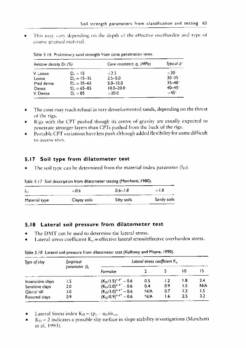
Soil s trength p a ram e te rs f ro m c lass i f ica t io n and tes t in g 63
• This mav vary depending on the depth of the effective overburden and type of coarse grained material.
Table 5 .16 Preliminary sand strength from cone penetration tests.
Relative density Dr (%) Cone resistance, qc (MPa) Typical (p
V. Loose D r < 15 <2.5 <30Loose D r = 15-35 2.5-5.0 30-35Med dense D r = 35-65 5.0-10.0 35-40Dense D r = 65-85 10.0-20.0 40-45V. Dense D r >85 >20.0 >45
• The cone may reach refusal in very dense/cemented sands, depending on the thrust of the rigs.
• Rigs with the CPT pushed though its centre of gravity are usually expected to penetrate stronger layers than CPTs pushed from the back of the rigs.
• Portable C P T variations have less push although added flexibility for some difficult to access sites.
5.17 Soil type from di la tom eter test• T h e soil type ca n be de te rm in ed fr o m the mater ia l in d e x p a r a m e te r ( Id ).
Table 5 .1 7 Soil description from dilatometer testing (Marchetti, 1980).
In < 0.6 0 .6-1 .8 > 1 .8
Material type Clayey soils Silty soils Sandy soils
5.18 Latera l soil pressure from d i la to m eter test• The D M T can be used to determine the lateral stress.• Lateral stress coefficient K() = effective lateral stress/effective overburden stress.
Table 5.18 Lateral soil pressure from dilatometer test (Kulhawy and Mayne, 1990).
Type o f clay Empiricalparameter
Lateral stress coefficient K 0
Formulae 2 5 10 15
Insensitive clays 1.5 (KD/I.5 )°47 - 0 .6 0.5 1.2 1.8 2.4Sensitive clays 2.0 (KD/2.0)°4 - 0 .6 0.4 0.9 1.5 N/AGlacial till 3.0 (Kd/3.0)° 47 - 0.6 N/A 0.7 1.2 1.5Fissured clays 0.9 (Kd/0.9)0 4" - 0.6 N/A 1.6 2.5 3.2
• Lateral Stress index Kp = (p„ - uo)/avo.• K d < 2 indicates a possible slip surface in slope stability investigations (Marchetti
et al, 1993) .
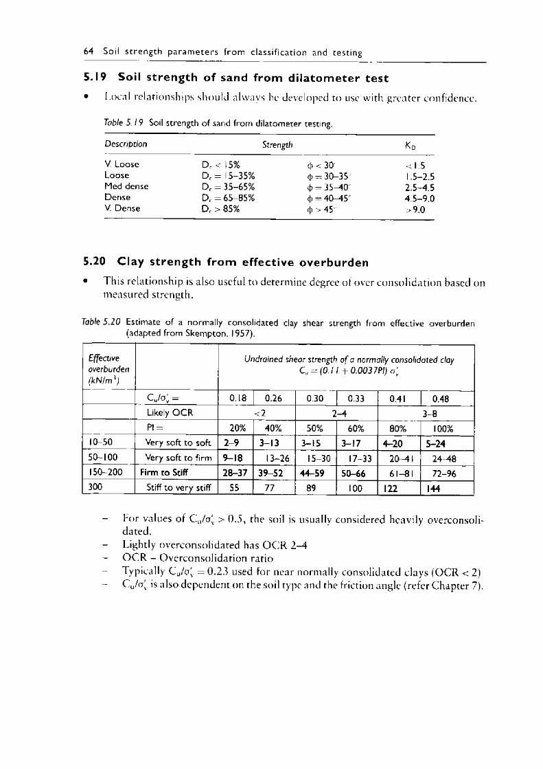
5.19 Soil strength of sand from di latometer test• Local relationships should always he developed to use with greater confidence.
64 Soil s t reng th p a ra m e te rs f ro m c lass i f ica t ion and testing
Table 5 .19 Soil strength of sand from dilatometer testing.
Description Strength K d
V. Loose D r < 15% ((><30 <1.5Loose D r = 15-35% (|> = 30-35 1.5-2.5Med dense D r = 35-65% c|> = 35-^0 2.5-4.5Dense D r = 65-85% <\) = 40—45 4.5-9.0V. Dense D r > 85% 4> > 45 >9.0
5.20 C lay strength from effective overburden• 1 his relationship is also useful to determine degree of over consolidation based on
measured strength.
Table 5 .20 Estimate of a normally consolidated clay shear strength from effective overburden (adapted from Skempton, 1957).
Effectiveoverburden(kN /m ')
Undrained shear strength o f a normally consolidated clay Cu = (0.11 -f- 0.003 7PI)
C u/o'v = 0.18 0.26 0.30 0.33 0.41 0.48Likely O C R <2 2-4 3-8Pl = 20% 40% 50% 60% 80% 100%
10-50 Very soft to soft 2-9 3-13 3-15 3-17 4-20 5-2450-100 Very soft to firm 9-18 13-26 15-30 17-33 20-41 24—48150-200 Firm to Stiff 28-37 39-52 44-59 50-66 61-81 72-96300 Stiff to very stiff 55 77 89 100 122 144
- For values of C Jo[, > 0 .5 , the soil is usually considered heavily overconsolidated.
- Lightly overconsolidated has O C R 2 - 4- O C R - Overconsolidation ratio- Typically C u/a'. = 0 .2 3 used for near normally consolidated clays (OCR < 2)
C Jo[. is also dependent on the soil type and the friction angle (refer Chapter 7).
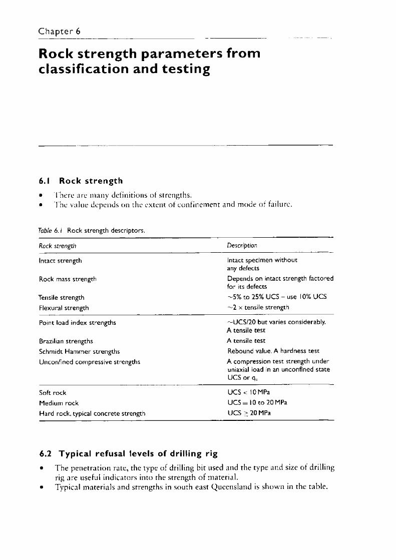
C hapter 6
Rock strength param eters from classification and testing
6.1 Rock strength• There are many definitions of strengths.• The value depends on the extent of confinement and mode of failure.
Table 6. / Rock strength descriptors.
Rock strength Description
Intact strength Intact specimen without any defects
Rock mass strength Depends on intact strength factored for its defects
Tensile strength -5 % to 25% U CS - use 10% U CSFlexural strength ~2 x tensile strength
Point load index strengths ^UCS/20 but varies considerably. A tensile test
Brazilian strengths A tensile testSchmidt Hammer strengths Rebound value. A hardness testUnconfined compressive strengths A compression test strength under
uniaxial load in an unconfined state U CS or qu
Soft rock U C S < 10 MPaMedium rock U CS = 10 to 20 MPaHard rock, typical concrete strength U CS > 20 MPa
6.2 Typ ica l refusal levels of drilling rig• The penetration rate, the type of drilling bit used and the type and size of drilling
rig are useful indicators into the strength of material.• Typical materials and strengths in south east Queensland is shown in the table.
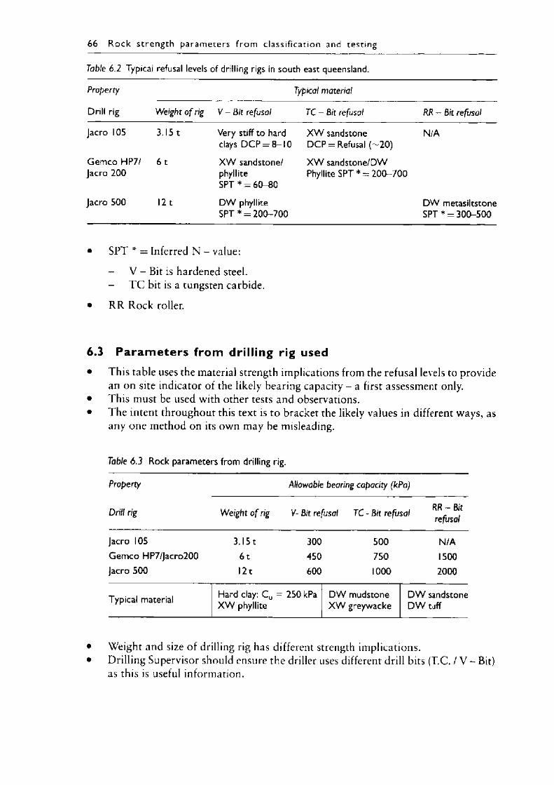
66 R o c k s treng th param ete rs f ro m c lass i f ica t ion and testing
Table 6.2 Typical refusal levels of drilling rigs in south east queensland.
Property Typical material
Drill rig Weight o f rig V - Bit refusal TC - Bit refusal RR - Bit refusal
Jacro 105 3.15 t Very stiff to hard clays D C P = 8-10
X W sandstone D CP = Refusal ( -2 0 )
N/A
Gem co HP7/ Jacro 200
6 t X W sandstone/ phylliteSPT * = 60-80
X W sandstone/DW Phyllite SPT * = 200-700
Jacro 500 12 t DW phyllite SPT * = 200-700
DW metasiltstone SPT * = 300-500
• SPT * = Inferred N - value:
- V - Bit is hardened steel.- T C bit is a tungsten carbide.
• R R Rock roller.
6.3 P a ram eters from drilling rig used• This table uses the material strength implications from the refusal levels to provide
an on site indicator of the likely bearing capacity - a first assessment only.• This must be used with other tests and observations.• The intent throughout this text is to bracket the likely values in different ways, as
any one method on its own may be misleading.
Table 6.3 Rock parameters from drilling rig.
Property Allowable bearing capacity (kPa)
Drill rig Weight o f rig V- Bit refusal TC - Bit refusal RR - Bit refusal
Jacro 105 3.151 300 500 N/AGem co HP7/Jacro200 6 t 450 750 1500Jacro 500 121 600 1000 2000
Typical material Hard clay: C u X W phyllite
= 250 kPa D W mudstone X W greywacke
D W sandstone D W tjff
• Weight and size of drilling rig has different strength implications.• Drilling Supervisor should ensure the driller uses different drill bits (T.C. / V - Bit)
as this is useful information.
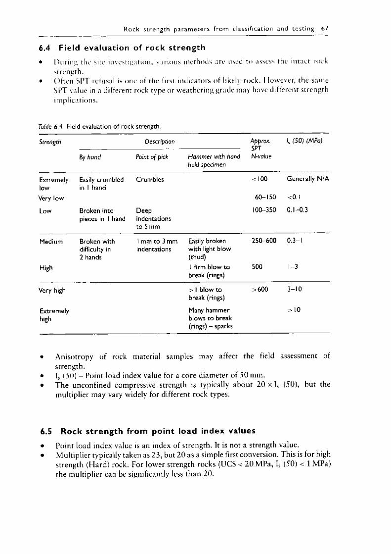
R o ck st reng th p a ra m e te rs f ro m c lass i f ica t ion and test ing 67
6.4 Field evaluation• During the sire investig
strength.• Often SPT refusal is on
SPT value in a different implications.
of rock strengthation, various methods are used to assess the intact rock
e of the first indicators of likely rock. However, the same rock type or weathering grade may have different strength
Table 6.4 Field evaluation of rock strength.
Strength Description Approx.SPTN-value
ls (50) (MPa)
By hand Point o f pick Hammer with hand held specimen
ExtremelylowVery low
Low
Easily crumbled in 1 hand
Broken into pieces in 1 hand
Crumbles
Deepindentations to 5 mm
<100
60-150
100-350
Generally N/A
<0.1
0.1-0.3
Medium
High
Broken with difficulty in 2 hands
1 mm to 3 mm indentations
Easily broken with light blow (thud)1 firm blow to break (rings)
250-600
500
0.3-1
1-3
Very high
Extremelyhigh
> 1 blow to break (rings)
Many hammer blows to break (rings) - sparks
>600 3-10
>10
• Anisotropy of rock material samples may affect the field assessment of strength.
• Is (50) - Point load index value for a core diameter of 50 mm.• The unconfined compressive strength is typically about 2 0 x Is (50), but the
multiplier may vary widely for different rock types.
6.5 Rock strength from point load index values• Point load index value is an index of strength. It is not a strength value.• Multiplier typically taken as 23, but 20 as a simple first conversion. This is for high
strength (Hard) rock. For lower strength rocks (UCS < 2 0 MPa, Is (50) < 1 MPa) the multiplier can be significantly less than 20.
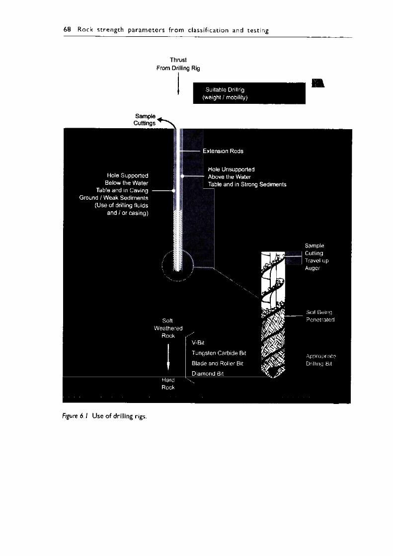
68 R ock s t reng th p a ra m e te rs f ro m c lass i f ica t ion and testing
Thrust From Drilling Rig
Suitable Drillrig (weight / mobility)
Sample ^ Cuttings
Hole Supported Below the Water
Table and in Caving Ground / Weak Sediments
(Use of drilling fluids and / or casing)
SoftWeathered
Rock
Extension Rods
Hole UnsupportedAbove the WaterTable and in Strong Sediments
§
Tungsten Carbide Bit Blade and Roller Bit Diamond Bit
ifll
Sample Cutting Travel up Auger
Figure 6. 1 Use of drilling rigs.
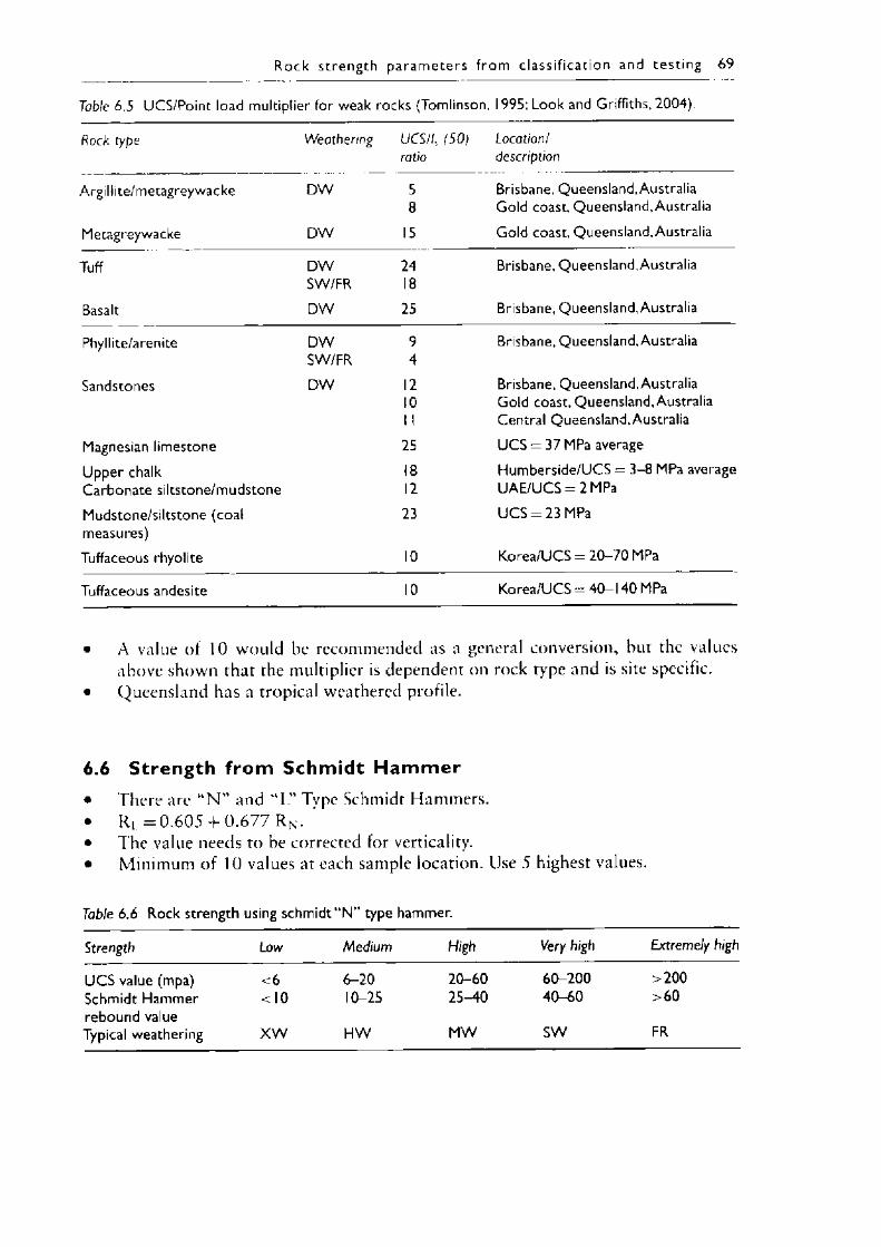
R o ck s trength p a ram ete rs f ro m c lass i f ica t ion and test ing 69
Table 6.5 UCS/Point load multipl ier for weak rocks (Tomlinson, 1995; Look and Griffiths. 2004).
Rock type Weathering UC.SH, (50) Location/ratio description
Argillite/metagreywacke DW 5 Brisbane, Queensland, Australia8 Gold coast, Queensland, Australia
Metagreywacke DW 15 Gold coast, Queensland, Australia
Tuff DW 24 Brisbane, Queensland, AustraliaSW/FR 18
Basalt D W 25 Brisbane, Queensland, Australia
Phyllite/arenite DW 9 Brisbane, Queensland, AustraliaSW/FR 4
Sandstones D W 12 Brisbane, Queensland, Australia10 Gold coast, Queensland, Australia1 1 Central Queensland, Australia
Magnesian limestone 25 U CS = 37 MPa average
Upper chalk 18 Humberside/UCS = 3-8 MPa averageCarbonate siltstone/mudstone 12 UAE/UCS = 2 MPaMudstone/siltstone (coal 23 U CS = 23 MPameasures)Tuffaceous rhyolite 10 Korea/UCS = 20-70 MPa
Tuffaceous andesite 10 Korea/UCS = 40-140 MPa
• A value of 10 would be recommended as a general conversion, but the values above shown that the multiplier is dependent on rock type and is site specific.
• Queensland has a tropical weathered profile.
6.6 Strength from Schm idt H a m m e r• There are “ N ” and “ I.” Type Schmidt Hammers.• R, = 0 . 6 0 5 + 0 . 6 7 7 R N.• The value needs to be corrected for verticality.• Minimum of 10 values at each sample location. Use 5 highest values.
Table 6.6 Rock strength using schmidt “N ” type hammer.
Strength Low Medium High Very high Extremely high
U C S value (mpa) <6 6-20 20-60 60-200 >200Schmidt Hammer <10 10-25 25-40 40-60 >60rebound valueTypical weathering x w H W MW SW FR
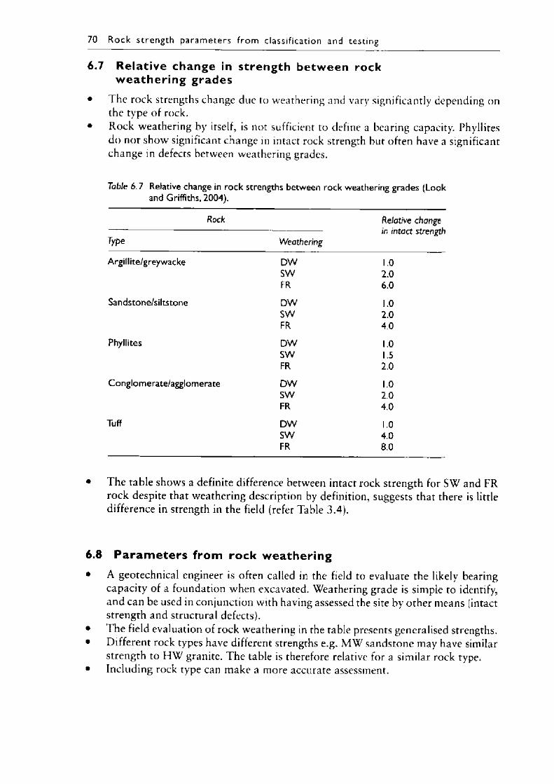
70 R o c k s treng th p a ra m e te rs f ro m c lass i f ica t ion and testing
6.7 Relative change in strength between rock w eather ing grades
• The rock strengths change due to weathering and vary significantly depending on the type of rock.
• Rock weathering by itself, is not sufficient to define a bearing capacity. Phyllites do not show significant change in intact rock strength but often have a significant change in defects between weathering grades.
Table 6.7 Relative change in rock strengths between rock weathering grades (Look and Griffiths, 2004).
Rock Relative change in intact strength
Type Weathering
Argillite/greywacke D W 1.0SW 2.0FR 6.0
Sandstone/siltstone DW 1.0SW 2.0FR 4.0
Phyllites DW 1.0SW 1.5FR 2.0
Conglomerate/agglomerate DW 1.0SW 2.0FR 4.0
Tuff DW 1.0SW 4.0FR 8.0
• The table shows a definite difference between intact rock strength for SW and FR rock despite that weathering description by definition, suggests that there is little difference in strength in the field (refer Table 3.4) .
6.8 P a ra m e te rs from rock weathering• A geotechnical engineer is often called in the field to evaluate the likely bearing
capacity of a foundation when excavated. Weathering grade is simple to identify, and can be used in conjunction with having assessed the site by other means (intact strength and structural defects).
• The field evaluation of rock weathering in the table presents generalised strengths.• Different rock types have different strengths e.g. M W sandstone may have similar
strength to FiW granite. The table is therefore relative for a similar rock type.• Including rock type can make a more accurate assessment.
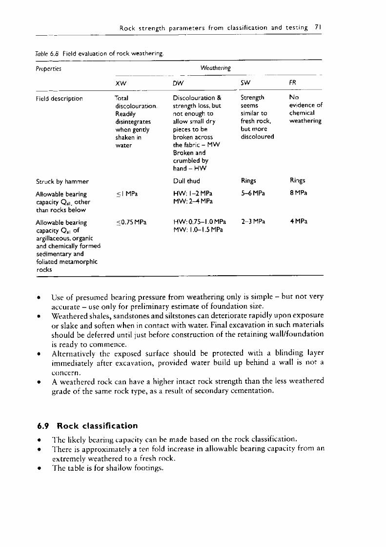
R o ck s treng th p a ram e te rs f ro m c lass i f ica t ion and te s t in g 71
Table 6.8 Field evaluation of rock weathering.
Properties Weathering
XW DW SW FR
Field description Totaldiscolouration. Readily disintegrates when gently shaken in water
Discolouration & strength loss, but not enough to allow small dry pieces to be broken across the fabric - MW Broken and crumbled by hand - H W
Strength seems similar to fresh rock, but more discoloured
N oevidence ofchemicalweathering
Struck by hammer Dull thud Rings Rings
Allowable bearing capacity Q an, other than rocks below
<1 MPa H W : 1-2 MPa MW: 2-4 MPa
5-6 MPa 8 MPa
Allowable bearing capacity Q an of argillaceous, organic and chemically formed sedimentary and foliated metamorphic rocks
<0.75 MPa HW : 0.75-1.0 MPa MW: 1.0-1.5 MPa
2-3 MPa 4 MPa
• Use of presumed bearing pressure from weathering only is simple - but not very accurate - use only for preliminary estimate of foundation size.
• Weathered shales, sandstones and siltstones can deteriorate rapidly upon exposure or slake and soften when in contact with water. Final excavation in such materials should be deferred until just before construction of the retaining wall/foundation is ready to commence.
• Alternatively the exposed surface should be protected with a blinding layer immediately after excavation, provided water build up behind a wall is not a concern.
• A weathered rock can have a higher intact rock strength than the less weathered grade o f the same rock type, as a result of secondary cementation.
6.9 Rock classification• The likely bearing capacity can be made based on the rock classification.• There is approximately a ten fold increase in allowable bearing capacity from an
extremely weathered to a fresh rock.• The table is for shallow footings.
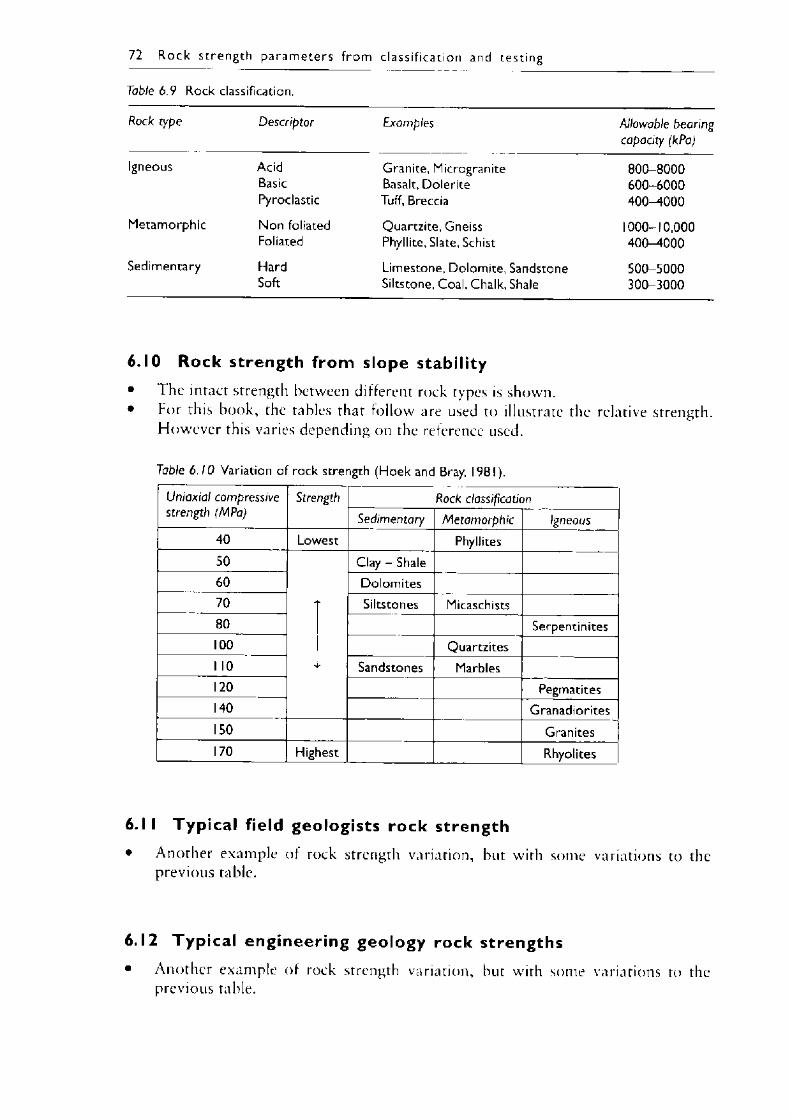
72 R ock strength param eters from classification and testing
Table 6.9 Rock classification.
Rock type Descriptor Examples Allowable bearing capacity (kPa)
Igneous AcidBasicPyroclastic
Granite, Microgranite Basalt, Dolerite Tuff, Breccia
800-8000600-6000400-4000
Metamorphic Non foliated Foliated
Quartzite. Gneiss Phyllite, Slate, Schist
1000-10,000400-4000
Sedimentary HardSoft
Limestone, Dolomite, Sandstone Siltstone, Coal, Chalk, Shale
500-5000300-3000
6.10 Rock strength from slope stability• The intact strength between different rock types is shown.• For this book, the tables that follow are used to illustrate the relative strength.
However this varies depending on the reference used.
Table 6.10 Variation of rock strength (Hoek and Bray, 1981).
Uniaxial compressive Strength Rock classificationstrength (MPa) Sedimentary Metamorphic Igneous
40 Lowest Phyllites50 Clay - Shale60 Dolomites70 - Siltstones Micaschists80 Serpentinites100 Quartzites1 10 J Sandstones Marbles120 Pegmatites140 Granadiorites150 Granites170 Highest Rhyolites
6.11 Typica l field geologists rock strength• Another example of rock strength variation, but with some variations to the
previous table.
6.12 Typica l engineering geology rock strengths• Another example of rock strength variation, but with some variations to the
previous table.
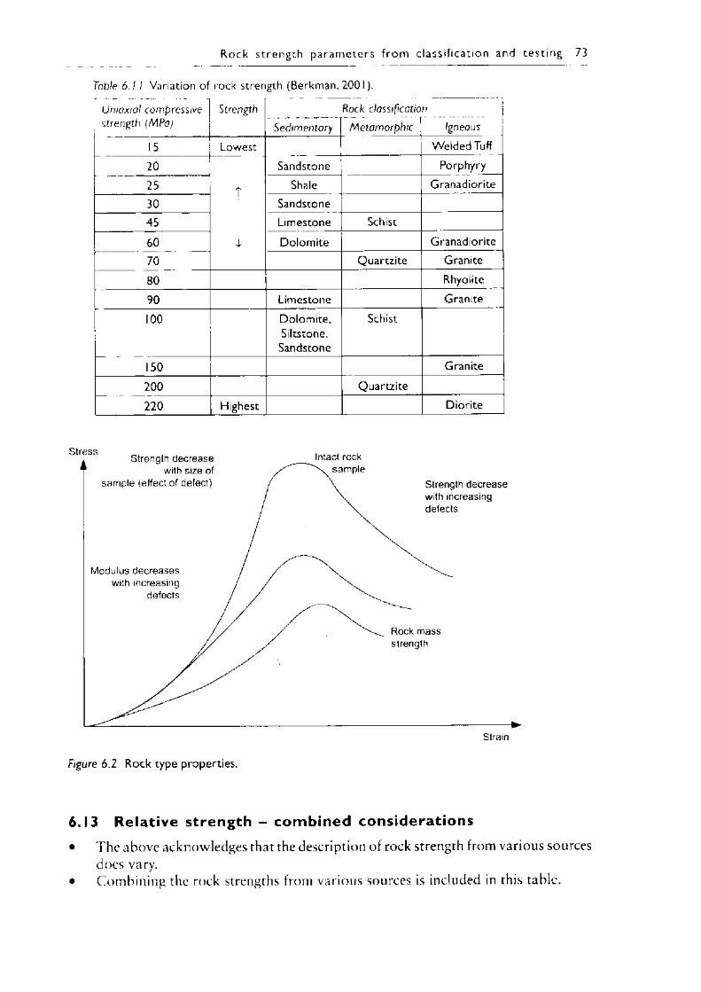
Table 6 .1 I Variation of rock strength (Berkman, 2001).
Uniaxial compressive [ Strength | Rock classification
R o c k s trength p a ra m e te rs f ro m c lass i f ica t io n and test ing 73
strength (MPa) Sedimentary Metamorphic Igneous
15 Lowest Welded Tuff20 Sandstone Porphyry25 Shale Granadiorite30 Sandstone45 Limestone Schist60 - Dolomite Granadiorite70 Quartzite Granite80 Rhyolite90 Limestone Granite100 Dolomite,
Siltstone.Sandstone
Schist
150 Granite200 Quartzite220 Highest Diorite
Figure 6.2 Rock type properties.
6.13 Relative strength - combined considerations• The above acknowledges that the description of rock strength from various sources
does vary.• Combining the rock strengths from various sources is included in this table.
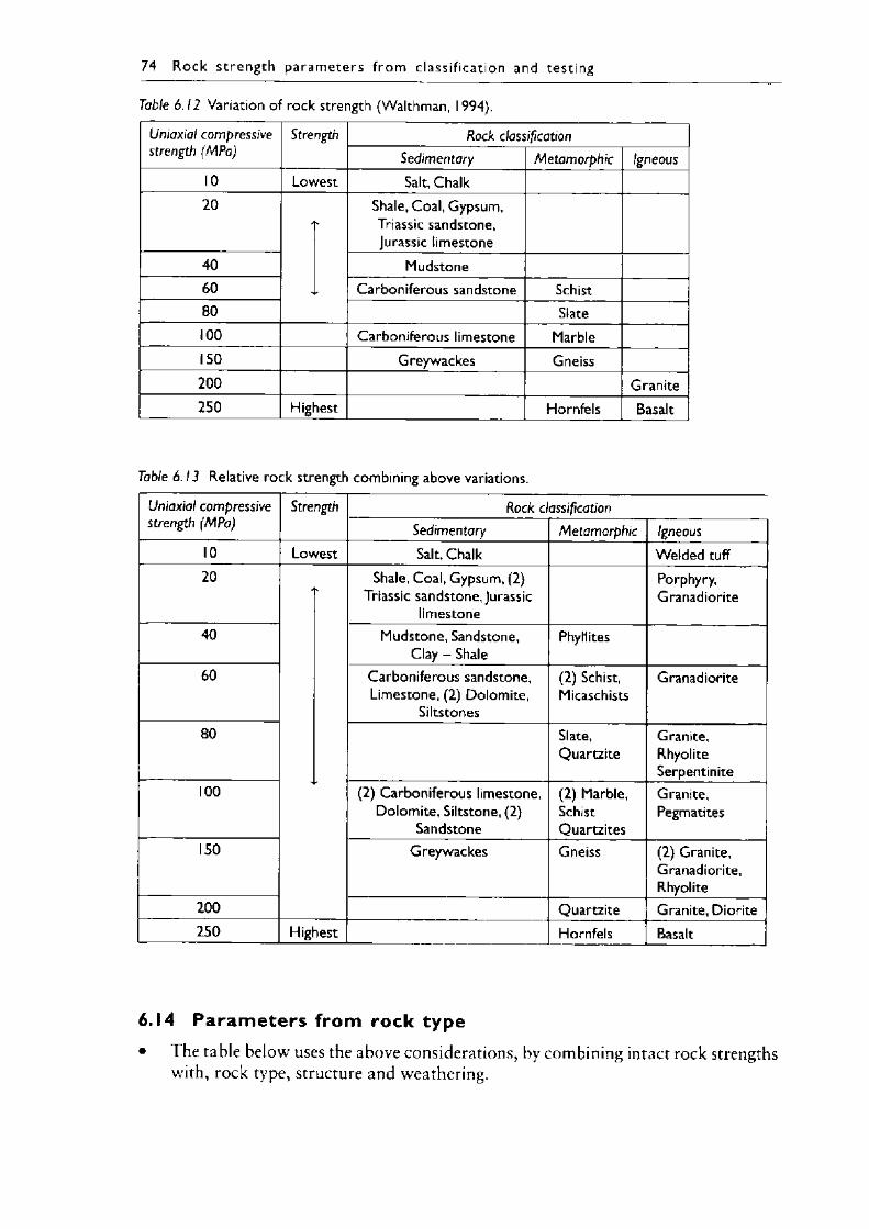
74 R ock s treng th p a ram e te rs f ro m c lass i f ica t ion and testing
Table 6.12 Variation of rock strength (Walthman, 1994).
Uniaxial compressive Strength Rock classificationstrength (MPa) Sedimentary Metamorphic Igneous
10 Lowest Salt, Chalk20 Shale, Coal, Gypsum,
Triassic sandstone, Jurassic limestone
40 Mudstone60 Carboniferous sandstone Schist80 Slate100 Carboniferous limestone Marble150 Greywackes Gneiss200 Granite250 Highest Hornfels Basalt
Table 6.13 Relative rock strength combining above variations.
Uniaxial compressive strength (MPa)
Strength Rock classificationSedimentary Metamorphic Igneous
10 Lowest Salt, Chalk Welded tuff20 Shale, Coal, Gypsum, (2)
Triassic sandstone, Jurassic limestone
Porphyry,Granadiorite
40 Mudstone, Sandstone, Clay - Shale
Phyllites
60 Carboniferous sandstone, Limestone, (2) Dolomite,
Siltstones
(2) Schist, Micaschists
Granadiorite
80 Slate,Quartzite
Granite,RhyoliteSerpentinite
100 (2) Carboniferous limestone, Dolomite, Siltstone, (2)
Sandstone
(2) Marble,SchistQuartzites
Granite,Pegmatites
150 Greywackes Gneiss (2) Granite,Granadiorite,Rhyolite
200 Quartzite Granite, Diorite250 Highest Hornfels Basalt
6.14 Pa ram eters from rock type• The table below uses the above considerations, by combining intact rock strengths
with, rock type, structure and weathering.
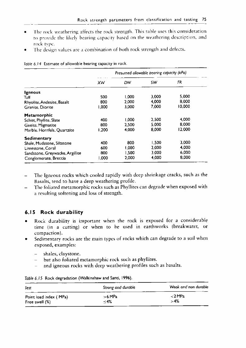
R o c k streng th p a ra m e te rs f ro m c lass i f ica t ion and test ing 75
• The rock weathering affects the rock strength. I his table uses this consideration to provide the likely bearing capacity based on the weathering description, and rock type.
• The design values are a combination of both rock strength and defects.
Table 6.14 Estimate of allowable bearing capacity in rock.
Presumed allowable bearing capacity (kPa)
X W DW S W FR
IgneousTuff 500 1,000 3,000 5,000Rhyolite, Andesite, Basalt 800 2,000 4,000 8,000Granite, Diorite 1,000 3,000 7,000 10,000
M etam orphicSchist, Phyllite, Slate 400 1,000 2,500 4,000Gneiss, Migmatite 800 2,500 5,000 8,000Marble, Hornfels, Quartzite 1,200 4,000 8,000 12,000
Sed im entaryShale, Mudstone, Siltstone 400 800 1,500 3,000Limestone, Coral 600 1,000 2,000 4,000Sandstone, Greywacke, Argillite 800 1,500 3,000 6,000Conglomerate, Breccia 1,000 2,000 4,000 8,000
- The Igneous rocks which cooled rapidly with deep shrinkage cracks, such as the Basalts, tend to have a deep weathering profile.
- The foliated metamorphic rocks such as Phyllites can degrade when exposed with a resulting softening and loss of strength.
6.15 Rock durability• Rock durability is important when the rock is exposed for a considerable
time (in a cutting) or when to be used in earthworks (breakwater, or compaction).
• Sedimentary rocks are the main types of rocks which can degrade to a soil when exposed, examples:
shales, claystone.but also foliated metamorphic rock such as phyllites.
- and igneous rocks with deep weathering profiles such as basalts.
Table 6 .15 Rock degradation (Walkinshaw and Santi, 1996).
Test Strong and durable Weak and non durable
Point load index ( MPa) >6 MPa <2 MPaFree swell (%) <4% >4%
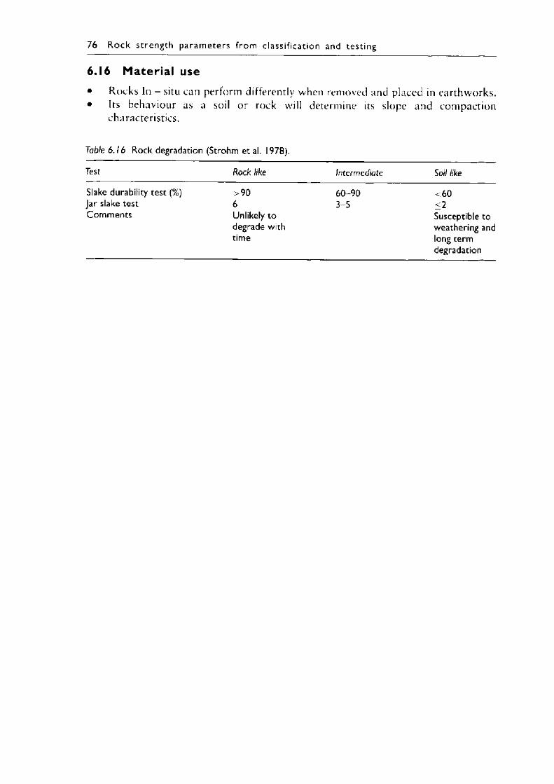
76 R o c k s trength p a ra m e te rs f ro m c lass i f ica t ion and testing
6.16 Material use• Rocks In - situ can perform differently when removed and placed in earthworks.• Its behaviour as a soil or rock will determine its slope and compaction
characteristics.
Table 6 .16 Rock degradation (Strohm et al. 1978).
Test Rock like Intermediate Soil like
Slake durability test (%) >90 60-90 <60Jar slake test 6 3-5 <2Comments Unlikely to
degrade with time
Susceptible to weathering and long term degradation
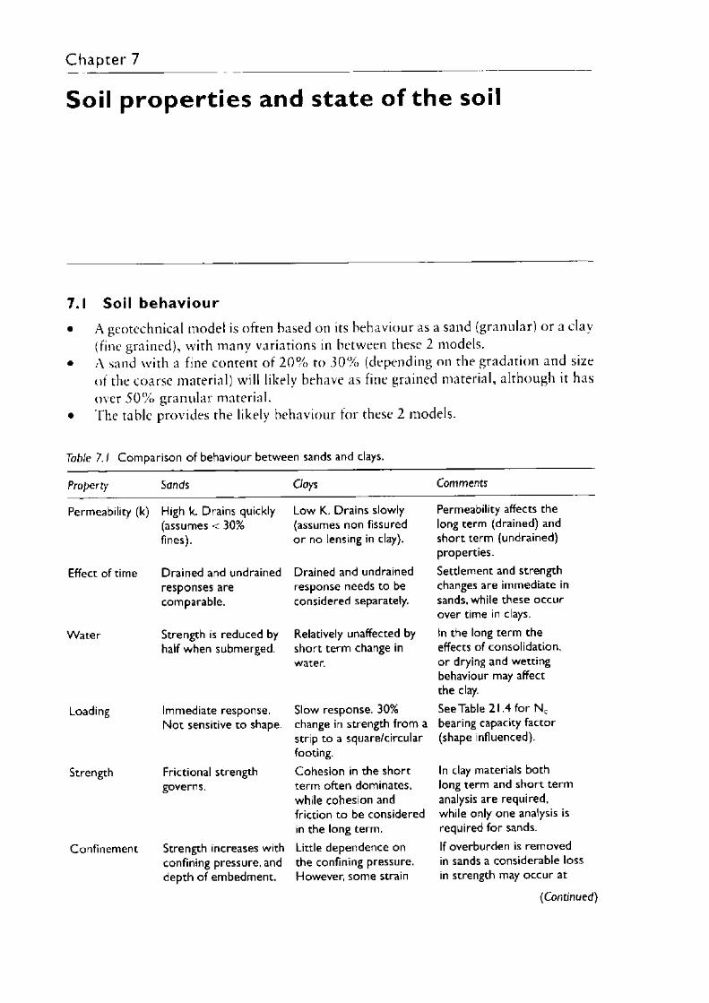
Soil properties and state of the soil
7.1 Soil behaviour• A geotcchnical model is often based on its behaviour as a sand (granular) or a clay
(fine grained), with many variations in between these 2 models.• A sand with a fine content of 2 0 % to 3 0 % (depending on the gradation and size
of the coarse material) will likely behave as fine grained material, although it hasover 5 0 % granular material.
• The table provides the likely behaviour for these 2 models.
Table 7. 1 Comparison of behaviour between sands and clays.
Property Sands Clays Comments
Permeability (k)
Effect of time
W ater
Loading
Strength
Confinement
High k. Drains quickly (assumes < 30% fines).
Drained and undrained responses are comparable.
Strength is reduced by half when submerged.
Immediate response. Not sensitive to shape.
Frictional strength governs.
Strength increases with confining pressure, and depth of embedment.
Low K. Drains slowly (assumes non fissured or no lensing in clay).
Drained and undrained response needs to be considered separately.
Relatively unaffected by short term change in water.
Slow response. 30% change in strength from a strip to a square/circular footing.Cohesion in the short term often dominates, while cohesion and friction to be considered in the long term.Little dependence on the confining pressure. However, some strain
Permeability affects the long term (drained) and short term (undrained) properties.Settlement and strength changes are immediate in sands, while these occur over time in clays.In the long term the effects of consolidation, or drying and wetting behaviour may affect the clay.See Table 2 1.4 for N c bearing capacity factor (shape influenced).
In clay materials both long term and short term analysis are required, while only one analysis is required for sands.If overburden is removed in sands a considerable loss in strength may occur at
(Continued)
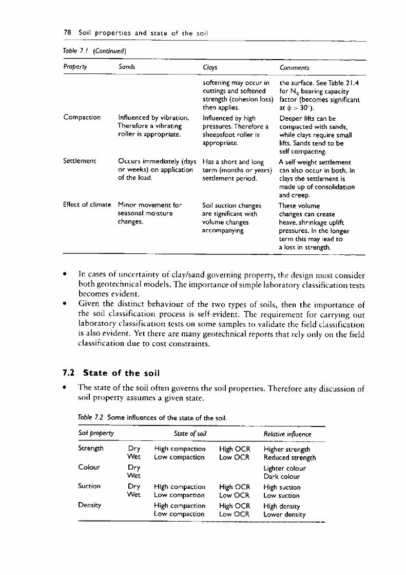
78 So il p ro p e r t ie s and s ta te of the soil
Table 7. 1 (Continued)
Property Sands Clays Comments
softening may occur in cuttings and softened strength (cohesion loss) then applies.
the surface. See Table 21.4 for Nq bearing capacity factor (becomes significantat 4) > 30°).
Compaction Influenced by vibration. Therefore a vibrating roller is appropriate.
Influenced by high pressures. Therefore a sheepsfoot roller is appropriate.
Deeper lifts can be compacted with sands, while clays require small lifts. Sands tend to be self compacting.
Settlement O ccurs immediately (days or weeks) on application of the load.
Has a short and long term (months or years) settlement period.
A self weight settlement can also occur in both. In clays the settlement is made up of consolidation and creep.
Effect of climate Minor movement for seasonal moisture changes.
Soil suction changes are significant with volume changes accompanying.
These volume changes can create heave, shrinkage uplift pressures. In the longer term this may lead to a loss in strength.
• In cases o f uncertainty of clay/sand governing property, the design must consider both geotechnical models. The importance of simple laboratory classification tests becomes evident.
• Given the distinct behaviour of the two types of soils, then the importance of the soil classification process is self-evident. The requirement for carrying out laboratory classification tests on some samples to validate the field classification is also evident. Yet there are many geotechnical reports that rely only on the field classification due to cost constraints.
7.2 State of the soil• The state of the soil often governs the soil properties. Therefore any discussion of
soil property assumes a given state.
Table 7.2 Some influences of the state of the soil.
Soil property State o f soil Relative influence
Strength D ryW et
High compaction Low compaction
High O C R Low O C R
Higher strength Reduced strength
Colour D ryW et
Lighter colour Dark colour
Suction DryW et
High compaction Low compaction
High O C R Low O C R
High suction Low suction
Density High compaction Low compaction
High O C R Low O C R
High density Lower density
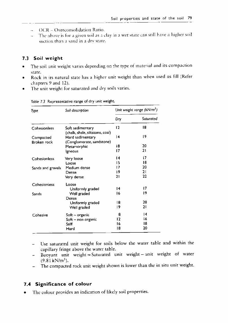
- O C R - Overconsolidation Ratio.- The above is for a given soil as a clay in a wet state can still have a higher soil
suction than a sand in a dry state.
7.3 Soil weight• The soil unit weight varies depending on the type of material and its compaction
state.• Rock in its natural state has a higher unit weight than when used as fill (Refer
chapters 9 and 12).• The unit weight for saturated and dry soils varies.
Soil p ro p e r t ie s and s ta te o f th e so il 79
Table 7.3 Representative range of dry unit weight.
Type Soil description Unit weight range (kN/'m3)
Dry Saturated
Cohesionless Soft sedimentary 12 18
Compacted(chalk, shale, siltstone, coal) Hard sedimentary 14 19
Broken rock (Conglomerate, sandstone) Metamorphic 18 20Igneous 17 21
Cohesionless Very loose 14 17Loose 15 18
Sands and gravels Medium dense 17 20Dense 19 21Very dense 21 22
Cohesionless LooseUniformly graded 14 17
Sands Well graded 16 19Dense
Uniformly graded 18 20Well graded 19 21
Cohesive Soft - organic 8 14Soft - non organic 12 16Stiff 16 18Hard 18 20
- Use saturated unit weight for soils below the water table and within the capillary fringe above the water table.
- Buoyant unit weight = Saturated unit weight — unit weight of water (9.81 kN/m3).
- The compacted rock unit weight shown is lower than the in situ unit weight.
7.4 Signif icance of colour• The colour provides an indication of likely soil properties.
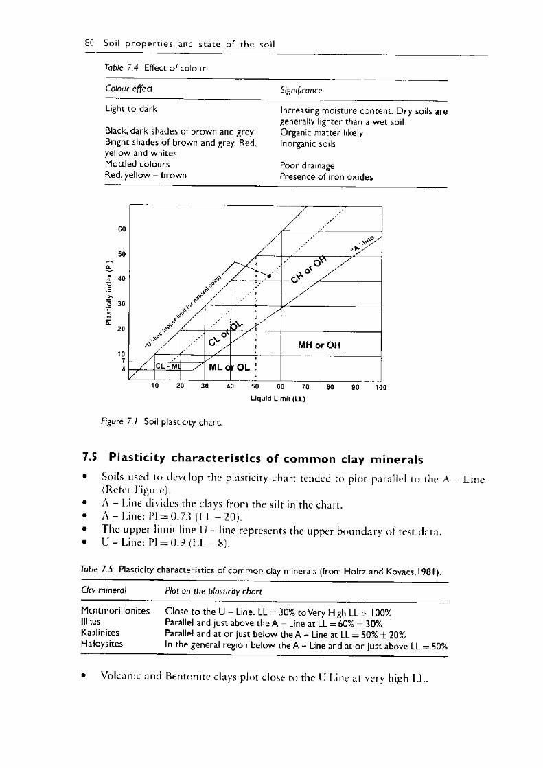
80 So il p ro p e r t ie s and s ta te of the s
Table 7.4 Effect of colour.
Colour effect
Light to dark
Black, dark shades of brown and grey Bright shades of brown and grey. Red, yellow and whites Mottled colours Red, yellow - brown
Significance
Increasing moisture content. Dry soils are generally lighter than a wet soil Organic matter likely Inorganic soils
Poor drainage Presence of iron oxides
Liquid Limit (LL)
Figure 7 .1 Soil plasticity chart.
7.5 Plastic ity character is t ics of common clay m inerals• Soils used to develop the plasticity chart tended to plot parallel to the A - Line
(Refer Figure).• A - Line divides the clays from the silt in the chart.• A - Line: PI = 0 .73 (LL - 2 0 ) .• I he upper limit line U - line represents the upper boundary of test data.• U - Line: PI = 0 .9 (LL - 8).
Tabe 7.5 Plasticity characteristics of common clay minerals (from Holtz and Kovacs, 19 8 1).
Clcv mineral Plot on the plasticity chart
McntmorilloniteslllitesKa^linitesHaloysites
Close to the U - Line. L L = 30% to Very High LL > 100%Parallel and just above the A - Line at LL = 60% ± 30%Parallel and at or just below the A - Line at LL = 50% ± 20%In the general region below the A - Line and at or just above LL = 50%
• Volcanic and Bentonite clays plot close to the U Line at very high LI
7.6 W e i g h t e d p l a s t i c i t y i ndex• The plasticity index bv itself can be misleading, as the test is carried out on the (\>
passing the 425 micron sieve, le any sizes greater than 425 |i m is discarded. I here have been cases when a predominantly “ rocky/granular” site has a high PI test results with over 7 5 % of the material discarded.
• The weighted plasticity index (WPl) considers the % of material used in the test.• WPl = PI x % passing the 425 micron sieve.
Soil p ro p e r t ie s and state o f the so il 81
Table 7.6 Weighted plasticity index classification (Look, 1994).
Volume change classification Weighted plasticity index %
Very low <1200Low 1200-2200Moderate 2200-3200High 3200-5000Very high >5000
7.7 Effect of grading• The grading affects the strength, permeability and density of soils.• Different grading requirements apply to different applications.
Table 7.7 Effect of grading.
Grading Benefits Application Comments
Well graded Low porosity with a Structural concrete, Well graded U > 5 andlow permeability. to minimize cement
contentC = 1 to 3
Uniformly graded Single sized or open - Preferred for Uniform grading U < 2graded aggregate has high porosity with a high permeability.
drainage Moderate grading:2 < U < 5. Open graded identified by their nominal size through which all of nearly all of material ( D 9 0 )
P (%) = (D/Dmax)n x 100 Maximum density Road base/sub - base n = 0.5 (Fullers curves)P - % passing size D (mm)
specification grading D max = maximum particle size
Well graded Increased friction Higher bearing Most commonangle capacity application
• D 90 = 19 mm is often referred to as 20 mm drainage gravel.• D90 = 9.5 mm is often referred to as 10 mm drainage gravel.
7.8 Effective fr ict ion of granular soils• The friction depends on the size and type of material, its degree of compaction
and grading.
82 Soil p ro p e r t ie s and s ta te of the soil
Table 7.8 Typical friction angle of granular soils.
Type Description/state Friction angle (degrees)
Cohesionless Soft sedimentary (chalk, shale, siltstone, coal) 30—40Compacted Hard sedimentary (conglomerate, sandstone) 35-45Broken rock Metamorphic 35-45
Igneous 40-50Cohesionless Very loose/loose 30-34Gravels Medium dense 34-39
Dense 39—44Very dense 44-49
Cohesionless Very loose/loose 27-32Sands Medium dense 32-37
Dense 37—42Very dense 42-47
Cohesionless LooseSands Uniformly graded 27-30
Well graded Dense
30-32
Uniformly graded 37-40Well graded 40—42
• Particle shape (rounded vs angular) also has an effect, and would change the above angles by about 4 degrees.
• When the percentage fines exceed 3 0 % , then the fines govern the strength.• Refer Figure 5.1.
7.9 Effective strength of cohesive soils• The typical peak strength is shown in the table.• Allowance should be made for long term softening of the clay, with loss o f effective
cohesion.• Remoulded strength and residual strength values would have a reduction in both
cohesion and friction.
Table 7.9 Effective strength of cohesive soils
Type Soil description/state Effective cohesion (kPa) Friction angle (degrees)
Cohesive Soft - organic 5-10 10-20Soft - non organic 10-20 15-25Stiff 20-50 20-30Hard 50-100 25-30
• Friction may increase with sand and stone content, and for lower plasticity clays.• When the percentage coarse exceeds 3 0 % , then some frictional strength is present.• In some cases (eg cuttings) the cohesion may not be able to be relied on for the
long term. The softened strength then applies.• Refer Figure 5.2.
Soil p ro p e r t ie s and state of the soil 83
7.10 Overconsolidat ion ratio• The Overconsolidation ratio (OCR) provides an indication of the stress history of
the soil. This is the ratio of its maximum past overburden pressure to its current overburden pressure.
• Material may have experienced higher previous stresses due to water table fluctuations or previous overburden being removed during erosion.
Table 7.10 Overconsolidation ratio.
Overconsolidation ratio (OCR) OCR = r c/ r 0
Preconsolidation pressure = Maximum stress ever placed on soil Present effective overburden Depth of overlying soil Effective unit weight Normally consolidated Lightly overconsolidated Heavily overconsolidated
• For aged glacial clays O C R = 1.5 — 2.0 for PI > 2 0 % (Bjerrum, 1972) .• Normally consolidated soils can strengthen with time when loaded.• Overconsolidated soils can have strength loss with time when unloaded (a cutting
or excavation) or when high strains apply.
7.11 Preconsol idat ion stress from cone penetration testing• The Preconsolidation stress is the maximum stress that has been experienced in
its previous history.• Current strength would have been based on its past and current overburden.
Table 7. / 1 Preconsolidation pressure from net cone tip resistance (from Mayne et al., 2002).
Net cone stress qr - P0 kPa 100 200 500 1000 1500 3000 5000
Preconsolidation pressure P'c kPa 33 67 167 333 500 1000 1667Excess pore water pressure Aui kPa 67 133 333 667 1000 2000 3333
• For intact clays only.• For fissured clays P£ = 2 0 0 0 to 6 0 0 0 with A ui = 6 0 0 to 3 0 0 0 kPa.• The electric piezocone (CPTu) only is accurate for this type of measurement. The
mechanical C P T is inappropriate.
7.12 Preconsol idat ion stress from D i la tom eter• The Dilatometer should theoretically be more accurate than the CPTu in measuring
the stress history. Flowever, currently the CPTu is backed by greater data history with a resulting greater prediction accuracy.
Pc
zy'O C R ~ I but < 1.5 O C R = 1.5-4 O C R > 4
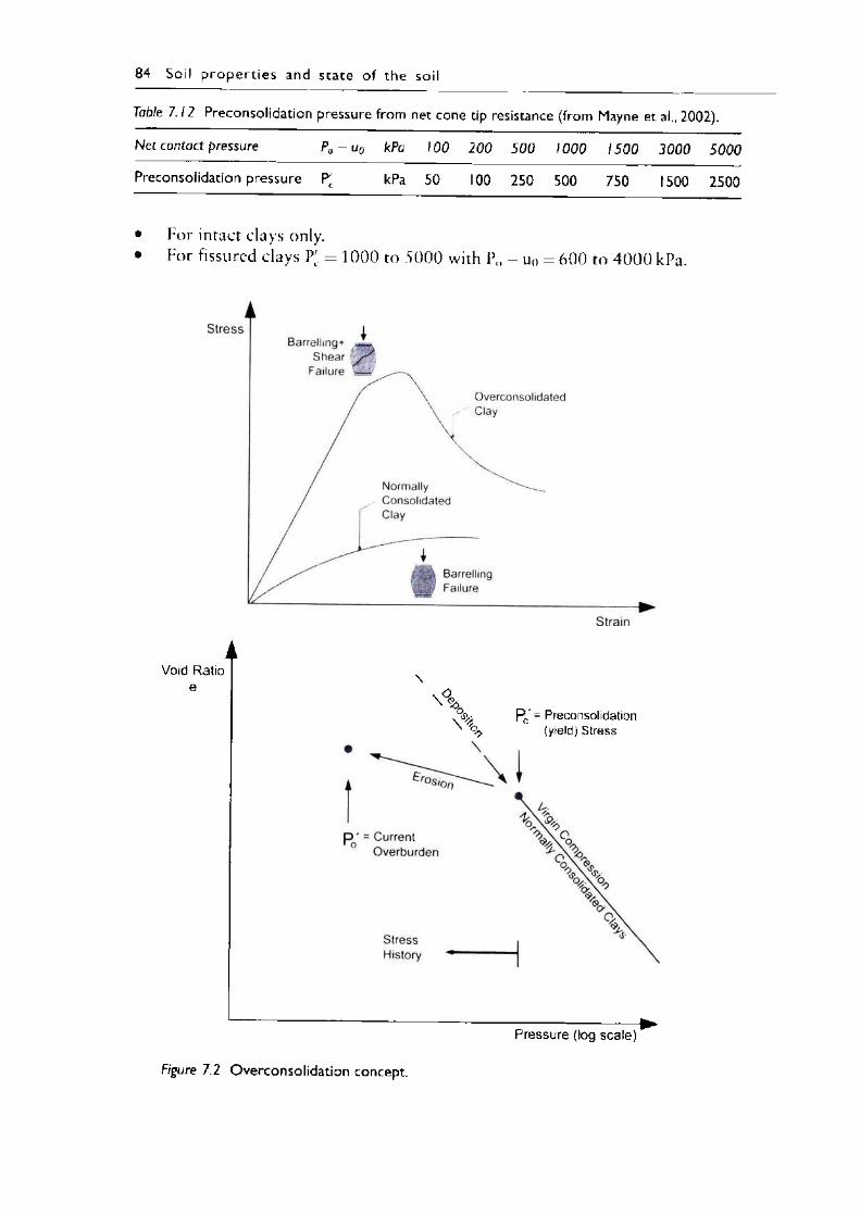
84 So il p ro p e r t ie s and s ta te o f the soil
Table 7.12 Preconsolidation pressure from net cone tip resistance (from Mayne et al„ 2002).
Net contact pressure 1 c o kPa 100 200 500 1000 1500 3000 5000
Preconsolidation pressure K kPa 50 100 250 500 750 1500 2500
For intact clays only.For fissured clays P' = 1000 to 5 0 0 0 with P„ - u(l = 6 0 0 to 4 0 0 0 kPa
Void Ratio e
A x R = Preconsolidation\ 'n c (yield) Stress
Pressure (log scale)
Figure 7.2 Overconsolidation concept.
7.13 Preconsol idat ion stress from shear wave velocity• The shear wave velocity for low preconsolidation pressures would require near
surface (Rayleigh) waves to be used.
Soil p ro p e r t ie s and s ta te o f th e so il 85
Table 7.13 Preconsolidation pressure from shear wave velocity (from Mayne et al., 2002).
Shear wave velocity Vs m/s 20 40 70 100 150 250 500
Preconsolidation pressure P' kPa 9 24 55 92 168 355 984
• For intact clays only• For fissured clays PJ. = 2 0 0 0 to 4 0 0 0 with V s = 150 to 4 0 0 m/s
7.14 O v e r consolidation ratio from D i la tom eter• Many correlation exists for O C R to dilatometer measurement of K n• K[> = 1.5 for a naturally deposited sand (Normally Consolidated)• K d = 2 for a Normally Consolidated clays• O C R = (0.5 Kn) ^ (Kulhawy and Mayne, 1990)• Table is for insensitive clays only
Table 7.14 O ver consolidation from dilatometer testing using the above relationship.
k d = I .5 -3 .0 2.5-6 3-8
oI 8-2 0 12-35 2 0 -5 0
O C R 1 2 3 5 10 20 30
• For intact clays only• For fissured clays O C R = 25 to 80 with K d = 7 to 20.
7.15 Latera l soil pressure from D i la to m eter test• The Dilatometer is useful to determine the stress history and degree of over
consolidation of a soil.
Table 7.15 Lateral soil pressure from Dilatometer test (Kulhawy and Mayne, 1990).
Type o f clay Empirical parameter fi0
Over consolidation ratio (OCR)
Formulae 2 5 10 15
Insensitive clays 0.5 (KD * 0.5)156 1.0 4.2 12 23Sensitive clays 0.35 (K d * 0.35)156 N/A 2.4 7 13Glacial till 0.27 (KD * 0 .2 7 ) '56 N/A 1.6 4.7 9Fissured clays 0.75 (K d * 0.75)156 1.9 7.9 23 44
86 So il p ro p e r t ie s and s ta te o f the soil
• K d — 2 or less then the soil is normally consolidated. A useful indicator in determining the slip zones in clays.
• Parameter pG used in the formulae shown.
7.16 O v e r consolidation ratio from undrained strength ratio and fr ict ion angles
• The friction angle o f the soil influences the O C R of the soil.• Sensitive CH clays are likely to have a lower friction angle.• CL sandy clays are likely to have the 30 degree friction angles.• Clayey sands are likely to have the higher friction angles.
Table 7.16 O ver consolidation from undrained strength ratio (after Mayne et al., 2001).
Culcf'v 0.2 0.22 0.3 0.4 0.5 0.7 1.0 1.25 1.5 2.0
Friction angle Over consolidation ratio
20° 1.5 1.7 2.3 3.1 3.8 5 8 10 1 1 1530° 1.0 1.0 1.4 1.9 2.4 3.3 5 6 7 1040 1.0 1.0 1.0 1.4 1.7 2.4 3.5 4 5 7
• Applies for unstructured and uncemented clays.• Value of 0 . 2 2 highlighted in the table as this is the most common value typically
adopted.
7.17 O verco nso l id a t ion ratio from undrained strength ratio• I he undrained strength ratio is dependent on the degree of over consolidation.
Table 7 .17 Overconsolidation from undrained strength ratio (after Ladd et al., 1977).
Overconsolidationratio
OH Clays CH Clays CL Clays/silts
1 0.25 to 0.35 0.2 to 0.3 0.15 to 0.202 0.45 to 0.55 0.4 to 0.5 0.25 to 0.354 0.8 to 0.9 0.7 to 0.8 0.4 to 0.68 1.2 to 1.5 0.9 to 1.2 0.7 to 1.010 1.5 to 1.7 1.3 to 1.5 0.8 to 1.2
7.18 Sign posts along the soil suction pF scale• Soil suction occurs in the unsaturated state. It represents the state of the soil’s
ability to attract water.• Units are pF or KPa (negative pore pressure). P F = 1 + Log S (kPa).
Soil p ro p e r t ie s and s ta te o f th e so il 87
Table 7.18 Soil suction values (Gay and Lytton, 1972; Hillel, 1971).
Soil suction
pF kPa
State Soil-plant-atmosphere continuum
12
110
Liquid limitSaturation limit of soils in the field 15 kPa for lettuce
3 100 Plastic limit of highly plastic clays Soil/stem4 1,000 Wilting point of vegetation (pF = 4.5) Stem/leaf: 1500 kPa for citrus trees5 10,000 Tensile strength of water Atmosphere; 75% relative
6 100,000 Air dryhumidity (pF = 5.6) 45% Relative humidity
7 1,000,000 Oven dry
• Equilibrium moisture condition is related to equilibrium soil suction. Refer to section 13.
• Soil suction contributes to strength in the soil. However, this strength cannot be relied upon in the long term and is often not directly considered in the analysis.
7.19 Soil suction values for different m ater ia ls• The soil suction depends on the existing moisture content of the soil. This soil—
water retention relationship (soil water characteristic curve) does vary depending on whether a wetting or a drying cycle.
Table 7.19 Typical soil suction values for various soils (Braun and Kruijne, 1994).
Volumetric moisture content (%)
Soil suction (pF)
Sand Clay Peat
0 7.0 7.0 7.010 1.8 6.3 5.720 1.5 5.6 4.630 1.3 4.7 3.640 0.0 3.7 3.250 2.0 2.860 0.0 2.270 0.3
- Volumetric moisture content is the ratio of the volume of water to the total volume.
- Soils in its natural state would not experience the soil suction pF = 0, as this is an oven dried condition. Thus for all practical purpose the effect of soil suction in sands are small.
- Greater soil suction produces greater moisture potential change and possible movement/swell of the soil.
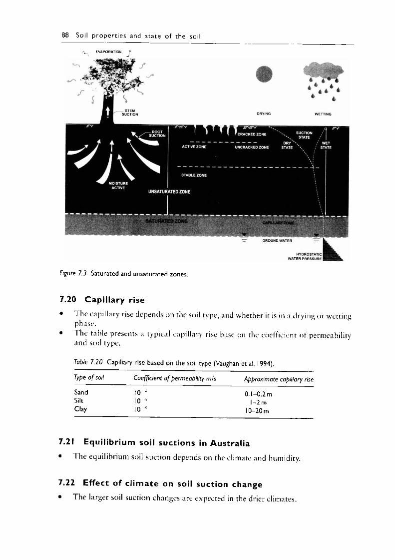
88 So il p ro p e r t ie s and sta te o f the soil
E V A P O R A T IO N
Figure 7.3 Saturated and unsaturated zones.
7.20 Cap i l la ry rise• The capillary rise depends on the soil type, and whether it is in a drying or wetting
phase.• I he table presents a typical capillary rise base on the coefficient of permeability
and soil type.
Table 7.20 Capillary rise based on the soil type (Vaughan et al, 1994).
Type o f soil Coefficient o f permeability m/s Approximate capillary rise
Sand 10 4 0.1-0.2 mSilt 10 6 1-2 mClay 10 « 10-20 m
7.21 Equil ibrium soil suctions in Australia• The equilibrium soil suction depends on the climate and humidity.
7.22 Effect of c l im ate on soil suction change• The larger soil suction changes are expected in the drier climates.
Soil p ro p e r t ie s and state of the so il 89
Tabic 7.21 Equilibrium soil suctions in Australia (N A A SR A , 1972: Australian Bureau of M eteorology).
Location Equilibrium soil suction (pF) Climatic environment Annual average rainfall (mm)
Darwin 2 to 3 Tropical 1666Sydney 3 to 4 Wet Coastal 1220Brisbane 3 to 4 Wet Coastal 1 189Townsville Tropical 1 136Perth 2 to 3 Temperate 869Melbourne 2 to 3 Temperate 661Canberra Temperate 631Adelaide 2 to 3 Temperate 553Hobart 2 to 3 Temperate 624Alice Springs >4.0 Semi - Arid 274
Table 7.22 Soil suction based on climate (AS 2870, 1996).
Climate description Soil suction change (A u , pF) Equilibrium soil suction, pF
Alpine/wet coastal 1.5 3.6Wet temperate 1.5 3.8Temperate 1.2-1.5 4.1Dry temperate 1.2-1.5 4.2Semi arid 1.5-1.8 4.4
7.23 Effect of c l im ate on active zones• The deeper active zones are expected in drier climates.• Thornwaithe Moisture Index (TMI) based on rainfall and evaporation
rates.
Table 7.23 Active zones based on climate (Walsh et al., 1998).
Climate description H $(metres) Thornwaithe moisture index (TM I)
Alpine/west coastal 1.5 >40W et temperate 1.8 10 to 40Temperate 2.3 - 5 to 10Dry temperate 3.0 -2 5 to - 5Semi arid 4.0 < -2 5
7.24 Effect of compaction on suction• The compaction affects the soil suction.• Soils compacted wet of optimum has less suction than those dry of
optimum.• Heavier compaction induces greater soil suction.
90 Soil p ro p e r t ie s and state of the soil
Table 7.24 Effect of compaction and suction (Bishop and Bjerrum, I960; Dineen et al., 1999).
Soil type Compaction Mo/sture content Soil suction
O M C = 9% -l0% MDD = 2.05 Mg/m3 Standard
2% Dry of OM C OM C2% Wet of OM C
150 kPa 30 kPa
< 10 kPaBentonite enriched soil Standard % Dry of OM C
OM C2% Wet of O M C
550 kPa 200 kPa 150 kPa
Modified % Dry of OM C OM C2% W et of OM C
1000 kPa
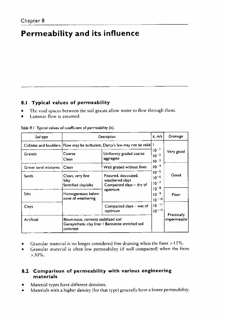
Chapter 8
Perm eability and its influence
8.1 Typica l values of permeabil ity• The void spaces between the soil grains allow water to flow through them.• Laminar flow is assumed.
Table 8 .1 Typical values of coefficient of permeability (k).
Soil type Description k, m/s Drainage
Cobbles and boulders Flow may be turbulent, Darcy’s law may not be valid
oo
oo
oo
oo
oo
oo
i i
i i
i i
i i
i i
i i
ro —
O
Very goodGravels CoarseClean
Uniformly graded coarse aggregate
Gravel sand mixtures Clean W ell graded without fines
GoodSands Clean, very fine SiltyStratified clay/silts
Fissured, desiccated, weathered clays Compacted clays - dry of optimum
Silts Homogeneous below zone of weathering
Poor
Clays Compacted clays - wet of optimum
PracticallyimpermeableArtificial Bituminous, cements stabilized soil
Geosynthetic clay liner / Bentonite enriched soil concrete
• Granular material is no longer considered free draining when the fines > 1 5 % .• Granular material is often low permeability (if well compacted) when the fines
> 3 0 % .
8.2 C o m p ar iso n of permeabil ity with various engineering m ater ia ls
• Material types have different densities.• Materials with a higher density (for that type) generally have a lower permeability.
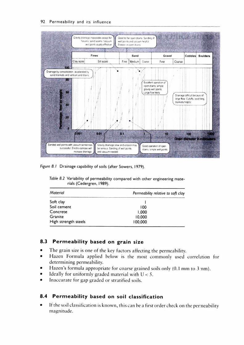
92 P e rm e a b i l i t y and its in f luence
mSm
m m m
__Gravity drainage impossible except for
fissures, sand seams Vacuum well point usually effective
Good to fair open drams Sanding of well points and vacuum helpful Erosion m open drams
>v
______ i_______ I v v
■■s
nFines Sand Gravel Cobbles Boulders
Clay sizes] Silt sizes Fine Medium Coarse Fine Coarse
i f ! 1 : .arge flow likely___
; .)] ,/
1 1 1 1 i f /
j f
Excellent operation of open drams, simple gravity well points
Drainage difficult becaus- of large flow Cutoffs void filing, blankets helpful
T i l ! | ,{•- f l i l
10 100Grain diameter In
v
Sanded well points with vacuum sometimes successful Electro-osmosis will
increase drainage’
Gravity drainage slow and erosion may be serious Sanding of well points and vacuum needed
Figure 8 .1 Drainage capability of soils (after Sowers, 1979).
Table 8.2 Variability of permeability compared with other engineering materials (Cedergren, 1989).
Material Permeability relative to soft clay
Soft clay 1Soil cement 100Concrete 1,000Granite 10,000High strength steels 100,000
8.3 Perm eabil i ty based on grain size• The grain size is one of the key factors affecting the permeability.• Hazen Formula applied below is the most commonly used correlation for
determining permeability.• Hazen’s formula appropriate for coarse grained soils only (0.1 mm to 3 rim).• Ideally for uniformly graded material with U < 5.• Inaccurate for gap graded or stratified soils.
8.4 Permeabil i ty based on soil classification• If the soil classification is known, this can be a first order check on the permeability
magnitude.
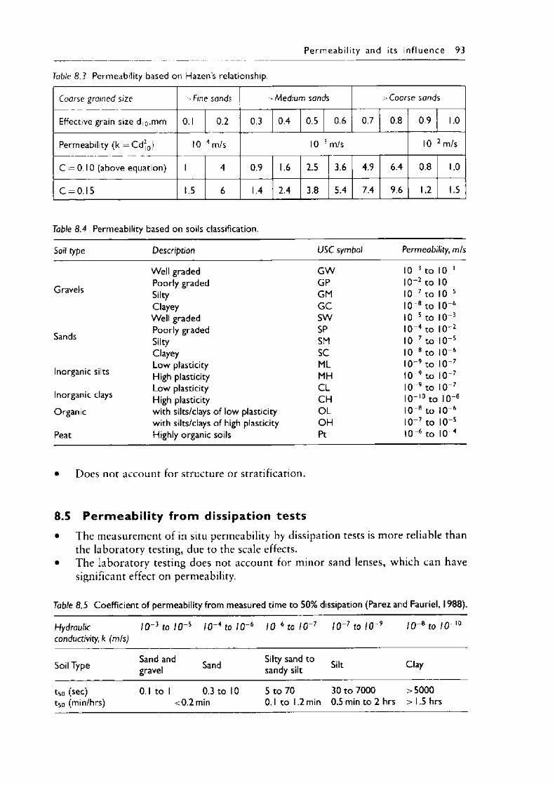
Pe rm eab i l i ty and its in f lu e n c e 93
Table 8.3 Permeability based on Hazen’s relationship.
Coarse grained size -> Fine sands -Medium sands > Coarse sands
Effective grain size d|0,mm 0.1 0.2 0.3 0.4 0.5 0.6 0.7 0.8 0.9 1.0
Permeability (k = Cd}0) 10 4 m/s Eo o ro 3 IS)
C = 0 .I0 (above equation) 1 4 0.9 1.6 2.5 3.6 4.9 6.4 0.8 1.0
C = 0 .I5 1.5 6 1.4 2.4 3.8 5.4 7.4 9.6 1,2 1.5
Table 8.4 Permeability based on soils classification.
Soil type Description USC symbol Permeability, m/s
Well graded G W 10 3 to 10 1
Gravels Poorly graded Silty
GPGM
10 2 to 10 10 7 to 10 5
Clayey G C 10 8 to 10 6Well graded SW 10 5 to 10 3
Sands Poorly graded SP 10 4 to 10 2Silty SM 10 7 to 10 5Clayey SC 10 8 to 10 6
Inorganic silts Low plasticity ML 10 9 to 10 7i / High plasticity MH 10 9 to 10 7
Inorganic clays Low plasticity C L 10 9 to 10 7High plasticity CH 10 10 to 10 8
Organic with silts/clays of low plasticity O L 10 8 to 10 6with silts/clays of high plasticity OH 10 7 to 10 5
Peat Highly organic soils Pt 10 6 to 10 4
• Does not account for structure or stratification.
8.5 Perm eabil i ty from dissipation tests• The measurement of in situ permeability by dissipation tests is more reliable than
the laboratory testing, due to the scale effects.• The laboratory testing does not account for minor sand lenses, which can have
significant effect on permeability.
Table 8.5 Coefficient of permeability from measured time to 50% dissipation (Parez and Fauriel, 1988).
Hydraulicconductivity, k (m/s)
10 3 to 10 5 10 4 to 10 6 10 6 to i O 1 10 7 to 10 9 10 8 to 10 10
Soil Type Sand and gravel Sand Silty sand to
sandy silt Silt Clay
tso (sec) t5o (min/hrs)
0.1 to 1 0.3 to 10 <0.2 min
5 to 70 0.1 to 1.2 min
30 to 7000 0.5 min to 2 hrs
>5000 > 1.5 hrs
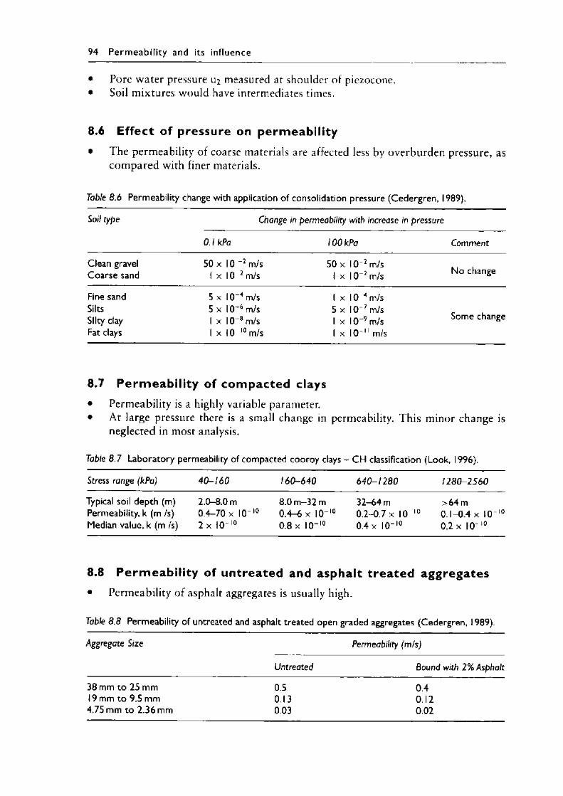
94 P e rm e a b i l i t y and its inf luence
Pore water pressure U2 measured at shoulder of piezocone. Soil mixtures would have intermediates times.
8.6 Effect of pressure on permeabil ity• The permeability of coarse materials are affected less by overburden pressure, as
compared with finer materials.
Table 8.6 Permeability change with application of consolidation pressure (Cedergren, 1989).
Soil type Change in permeability with increase in pressure
0.1 kPa lOOkPa Comment
Clean gravel 50 x 10 2 m/s 50 x 10 2 m/sCoarse sand 1 x 10 2 m/s 1 x 10"2 m/s No change
Fine sand 5 x 10 4 m/s 1 x 10 4 m/sSilts 5 x 10 6 m/s 5 x 10~7 m/sSilty clay 1 x 10 8 m/s 1 x I0 -9 m/s Some changeFat clays 1 x 10 10 m/s 1 x 10 11 m/s
8.7 Perm eab i l i ty of compacted clays• Permeability is a highly variable parameter.• At large pressure there is a small change in permeability. This minor change is
neglected in most analysis.
Table 8 .7 Laboratory permeability of compacted cooroy clays - CH classification (Look, 1996).
Stress range (kPa) 40-160 160-640 640-1280 1280-2560
Typical soil depth (m) 2.0-8.0 m 8.0 m-32 m 32-64 m >64 mPermeability, k (m Is) 0.4-70 x 10 10 0.4-6 x 10 10 0.2-0.7 x 10 10 0.1-0.4 x 10 10Median value, k (m /s) 2 x 10 10 0.8 x 10” 10 0.4 x 10 10 0.2 x 10 10
8.8 Perm eab i l i ty of untreated and asphalt t reated aggregates• Permeability of asphalt aggregates is usually high.
Table 8.8 Permeability of untreated and asphalt treated open graded aggregates (Cedergren, 1989).
Aggregate Size Permeability (m/s)
Untreated Bound with 2% Asphalt
38 mm to 25 mm 0.5 0.419 mm to 9.5 mm 0.13 0.124.75 mm to 2.36 mm 0.03 0.02
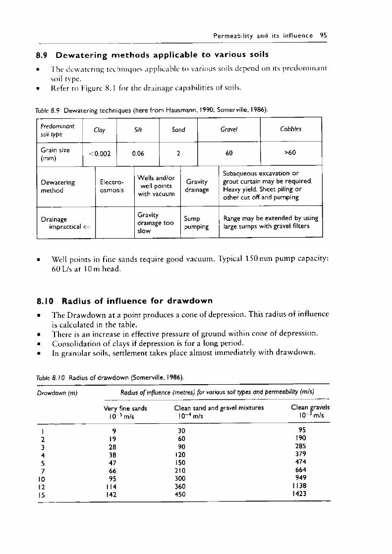
Pe rm eab i l i ty and its in f lu e n c e 95
8.9 D ewater ing methods applicable to various soils• The dewatering techniques applicable to various soils depend on its predominant
soil type.• Refer to Figure 8.1 for the drainage capabilities of soils.
Table 8.9 Dewatering techniques (here from Hausmann, 1990; Somerville, 1986).
Predominant soil type Clay Silt Sand Gravel Cobbles
Grain size (mm) < 0.002 0.06 2 60 >60
Dewateringmethod
Electroosmosis
Wells and/or well points
with vacuum
Gravitydrainage
Subaqueous excavation or grout curtain may be required. Heavy yield. Sheet piling or other cut off and pumping
Drainageimpractical <=
Gravity drainage too slow
Sumppumping
Range may be extended by using large sumps with gravel filters
• Well points in fine sands require good vacuum. Typical 150 mm pump capacity: 6 0 L/s at 10 m head.
8.10 Radius of influence for drawdown• The Drawdown at a point produces a cone of depression. This radius o f influence
is calculated in the table.• There is an increase in effective pressure of ground within cone of depression.• Consolidation o f clays if depression is for a long period.• In granular soils, settlement takes place almost immediately with drawdown.
Table 8 .10 Radius of drawdown (Somerville, 1986).
Drawdown (m) Radius o f influence (metres) for various soil types and permeability (m/s)
Very fine sands 10 5 m/s
Clean sand and gravel mixtures 10 4 m/s
Clean gravels 10 3 m/s
1 9 30 952 19 60 1903 28 90 2854 38 120 3795 47 150 4747 66 210 664
10 95 300 94912 1 14 360 1 13815 142 450 1423
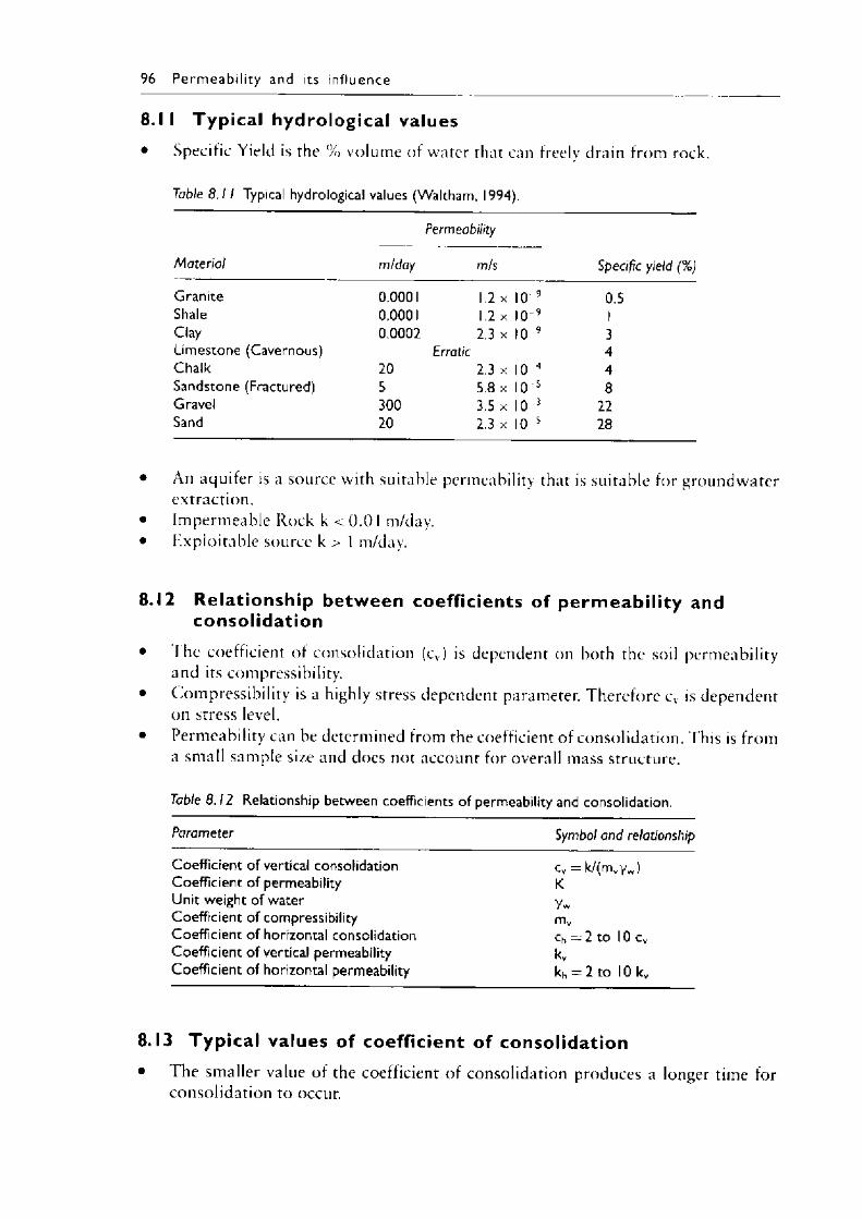
96 Perm eability and its influence
8.11 Typica l hydrological val ues• Specific Yield is the % volume of water that can freely drain from rod
Table 8.11 Typical hydrological values (Waltham, 1994).
Permeability
Material m/day m/s Specific yield (%)
Granite 0.0001 1.2 x 10 9 0.5Shale 0.0001 1.2 x 10 9 1Clay 0.0002 2.3 x 10 9 3Limestone (Cavernous) Erratic 4Chalk 20 2.3 x 10 4 4Sandstone (Fractured) 5 5.8 x 10 5 8Gravel 300 3.5 x 10 3 22Sand 20 2.3 x 10 5 28
• An aquifer is a source with suitable permeability that i:s suitable for grextraction.
• Impermeable Rock k < 0.01 m/day.• Exploitable source k > 1 m/day.
8.12 Relationship between coefficients of permeabil ity and consolidation
• The coefficient of consolidation (cv) is dependent on both the soil permeability and its compressibility.Compressibility is a highly stress dependent parameter. Therefore c v is dependent on stress level.Permeability can be determined from the coefficient of consolidation. This is from a small sample size and does not account for overall mass structure.
Table 8 .12 Relationship between coefficients of permeability and consolidation.
Parameter Symbol and relationship
Coefficient of vertical consolidation cv = k/(mvy jCoefficient of permeability KUnit weight of water YwCoefficient of compressibility mvCoefficient of horizontal consolidation ch — 2 to 10 cvCoefficient of vertical permeability kvCoefficient of horizontal permeability kh = 2 to 10 kv
8.13 Typ ica l values of coefficient of consolidation• The smaller value of the coefficient of consolidation produces a longer time for
consolidation to occur.
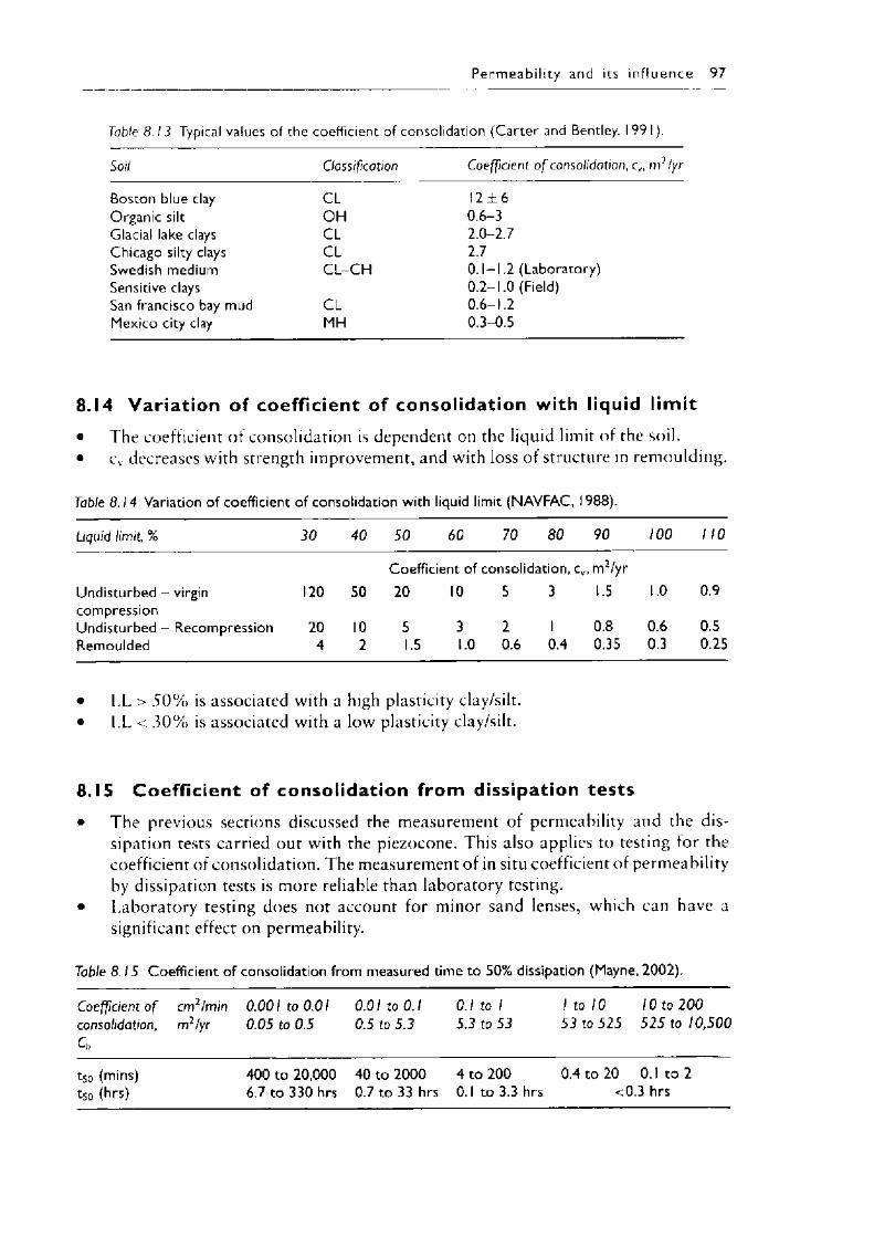
P e rm e a b i l i t y and its in f luence 97
Table 8.13 Typical values of the coefficient of consolidation (C a rte r and Bentley, 1991).
Soil Classification Coefficient o f consolidation, cv, m2/yr
Boston blue clay C L 12 ± 6Organic silt OH 0.6-3Glacial lake clays C L 2.0-2.7Chicago silty clays C L 2.7Swedish medium C L -C H 0.1-1.2 (Laboratory)Sensitive clays 0.2-1.0 (Field)San francisco bay mud CL 0.6-1.2Mexico city clay MH 0.3-0.5
8.14 Var iat ion of coefficient of consolidation with liquid limit• The coefficient o f consolidation is dependent on the liquid limit of the soil.• c v decreases with strength improvement, and with loss o f structure in remoulding.
Table 8.14 Variation of coefficient of consolidation with liquid limit (NAVFAC, 1988).
Liquid limit, % 30 40 50 60 70 80 90 100 110
Coefficient of consolidation, cv, m2/yrUndisturbed - virgin 120 50 20 10 5 3 1.5 1.0 0.9compressionUndisturbed - Recompression Remoulded
204
102
51.5
31.0
20.6
10.4
0.80.35
0.60.3
0.50.25
• LL > 5 0 % is associated with a high plasticity clay/silt.• LL < 3 0 % is associated with a low plasticity clay/silt.
8.15 Coeff ic ient of consolidation from dissipation tests• The previous sections discussed the measurement of permeability and the dis
sipation tests carried out with the piezocone. This also applies to testing for the coefficient of consolidation. The measurement of in situ coefficient of permeability by dissipation tests is more reliable than laboratory testing.
• Laboratory testing does not account for minor sand lenses, which can have a significant effect on permeability.
Table 8.15 Coefficient of consolidation from measured time to 50% dissipation (Mayne, 2002).
Coefficient o f cm2/min 0.001 to 0.01 0.01 to 0.1 0. 1 to 1 1 to 10 10 to 200consolidation, m2/yrch
0.05 to 0.5 0.5 to 5.3 5.3 to 53 53 to 525 525 to 10,500
t50 (mins) 400 to 20,000 40 to 2000 4 to 200 0.4 to 20 0.1 to 2t50 (hrs) 6.7 to 330 hrs 0.7 to 33 hrs 0. 1 to 3.3 hrs < 0.3 hrs
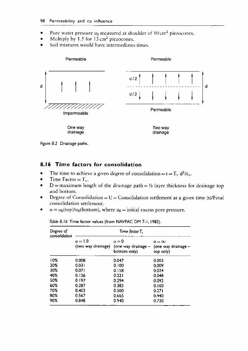
98 P e rm e a b i l i t y and its in f luence
• Pore water pressure 112 measured at shoulder of 1 0c m 2 piezocones.• Multiply by 1.5 for 15 cm2 piezocones.• Soil mixtures would have intermediates times.
Permeable
/ / / / / / / / / / / / / / /Impermeable
One way drainage
Figure 8.2 Drainage paths.
Permeable
d/2
d/2
Permeable
Two way drainage
8.16 T im e factors for consolidation• The time to achieve a given degree of consolidation = t = T v d2/cv.• Time Factor = T v.• D = maximum length of the drainage path = Vi layer thickness for drainage top
and bottom.• Degree of Consolidation = U = Consolidation settlement at a given time (t)/Final
consolidation settlement.• a = u q (top ) / u q ( bottom), where u q = initial excess pore pressure.
Table 8.16 Time factor values (from NAVFAC DM 7-1, 1982).
Degree o f consolidation
Time factor Tv
a = 1.0(two way drainage)
a = 0(one way drainage - bottom only)
a = 00(one way drainage - top only)
10% 0.008 0.047 0.00320% 0.031 0.100 0.00930% 0.071 0.158 0.02440% 0.126 0.221 0.04850% 0.197 0.294 0.09260% 0.287 0.383 0.16070% 0.403 0.500 0.27180% 0.567 0.665 0.44090% 0.848 0.940 0.720
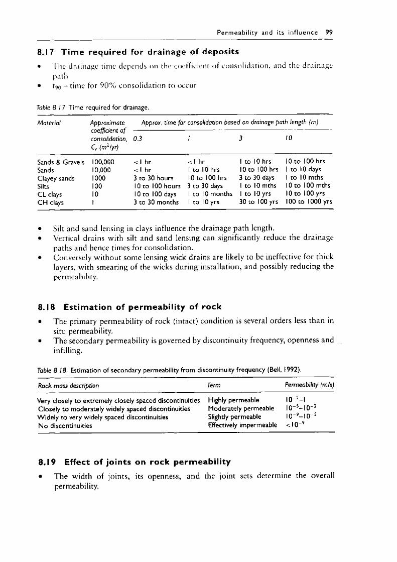
P e rm e a b i l i t y and its in f lu en ce 99
8.17 T im e required for drainage of deposits• The drainage time depends on the coefficient of consolidation, and the drainage
path• t9o - time for 9 0 % consolidation to occur
Table 8 .1 7 Time required for drainage.
Material Approximate Approx. time for consolidation based on drainage path length (m)coefficient o f consolidation, Cv (m2/yr)
0.3 / 3 10
Sands & Gravels 100,000 < 1 hr < 1 hr 1 to 10 hrs 10 to 100 hrsSands 10,000 < 1 hr 1 to 10 hrs 10 to 100 hrs 1 to 10 daysClayey sands 1000 3 to 30 hours 10 to 100 hrs 3 to 30 days 1 to 10 mthsSilts 100 10 to 100 hours 3 to 30 days 1 to 10 mths 10 to 100 mthsC L clays 10 10 to 100 days 1 to 10 months 1 to 10 yrs 10 to 100 yrsCH clays 1 3 to 30 months 1 to 10 yrs 30 to 100 yrs 100 to 1000 yrs
• Silt and sand lensing in clays influence the drainage path length.• Vertical drains with silt and sand lensing can significantly reduce the drainage
paths and hence times for consolidation.• Conversely without some lensing wick drains are likely to be ineffective for thick
layers, with smearing of the wicks during installation, and possibly reducing the permeability.
8.18 Est im ation of permeabil ity of rock• The primary permeability of rock (intact) condition is several orders less than in
situ permeability.• The secondary permeability is governed by discontinuity frequency, openness and
infilling.
Table 8 .18 Estimation of secondary permeability from discontinuity frequency (Bell, 1992).
Rock mass description Term Permeability (m/s)
Very closely to extremely closely spaced discontinuities Closely to moderately widely spaced discontinuities W idely to very widely spaced discontinuities No discontinuities
Highly permeable Moderately permeable Slightly permeable Effectively impermeable
10 2- l I0~5- I 0 2 10 9- IO 5 < I 0 ' 9
8.19 Effect of joints on rock permeabil ity• The width of joints, its openness, and the joint sets determine the overall
permeability.
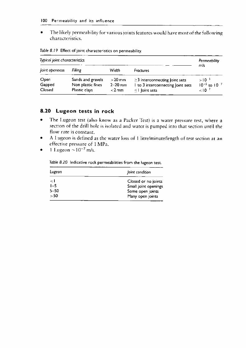
100 P e rm e a b i l i t y and its in f luence
The likely permeability for various joints features would have most of the following characteristics.
Table 8 .19 Effect of joint characteristics on permeability.
Typical joint characteristics Permeabilitym/s
Joint openness Filling Width Fractures
OpenGappedClosed
Sands and gravels Non plastic fines Plastic clays
>20 mm 2-20 mm <2 mm
>3 interconnecting Joint sets 1 to 3 interconnecting Joint sets < 1 Joint sets
>10 510 5 to 10 7 <10 7
8.20 Lugeon tests in rock• The Lugeon test (also know as a Packer Test) is a water pressure test, where a
section of the drill hole is isolated and water is pumped into that section until the flow rate is constant.
• A Lugeon is defined as the water loss of 1 litre/minute/length of test section at an effective pressure of 1 MPa.
• I Lugeon ~10'~7 m/s.
Table 8 .20 Indicative rock permeabilities from the lugeon test.
Lugeon Joint condition
<1 Closed or no joints1-5 Small joint openings5-50 Some open joints>50 Many open joints
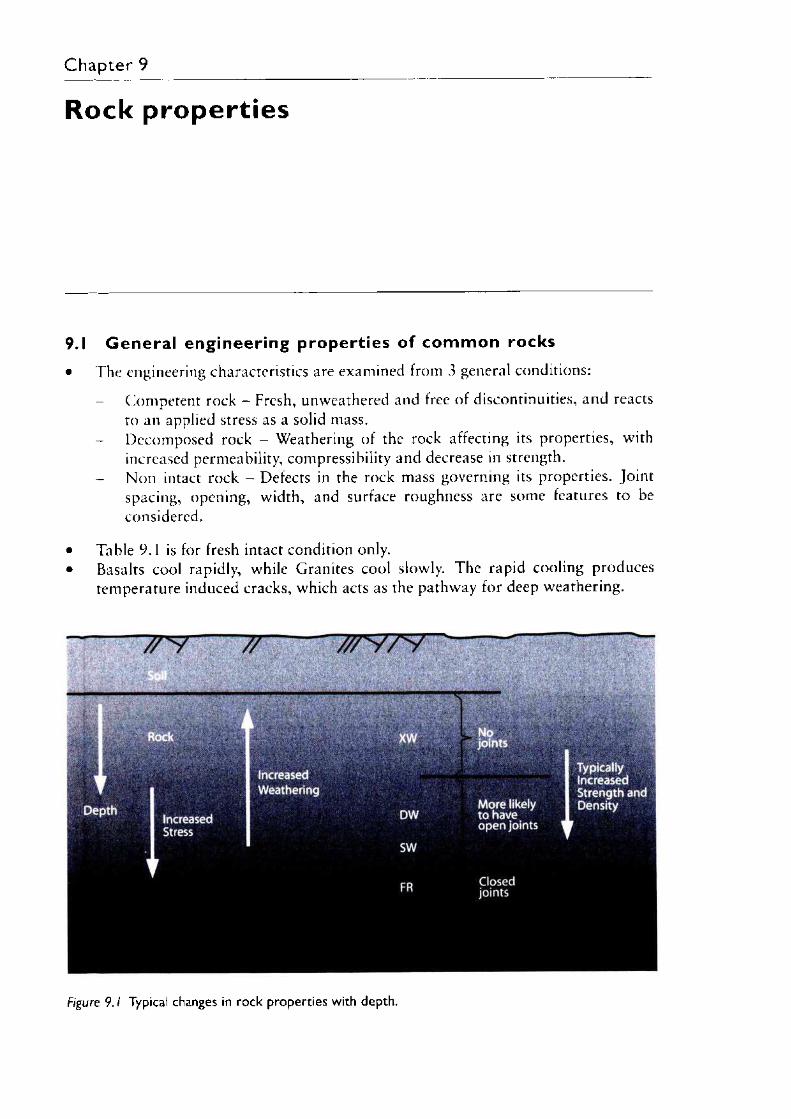
Ch ap ter 9
Rock properties
9.1 G enera l engineering propert ies of com m on rocks• The engineering characteristics are examined from 3 general conditions:
- Competent rock - Fresh, unweathered and free of discontinuities, and reacts to an applied stress as a solid mass.Decomposed rock - Weathering of the rock affecting its properties, with increased permeability, compressibility and decrease in strength.Non intact rock - Defects in the rock mass governing its properties. Joint spacing, opening, width, and surface roughness are some features to be considered.
• Table 9.1 is for fresh intact condition only.• Basalts cool rapidly, while Granites cool slowly. The rapid cooling produces
temperature induced cracks, which acts as the pathway for deep weathering.
Increased
Figure 9. 1 Typical changes in rock properties with depth.
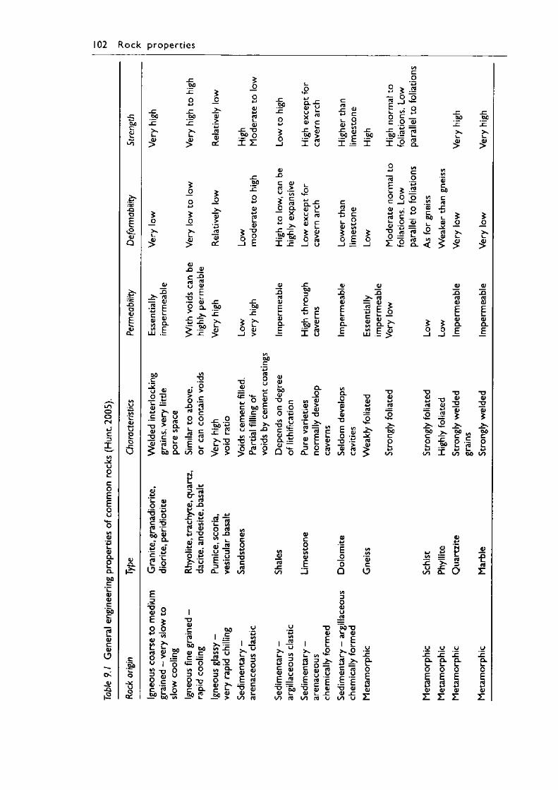
102 R o c k p ro p e r t ie s
-ctxoc<u
DuOJOX
2
J ZbO
In
bo QJ>wJ2qj
QJfOi_QJ-C X Ibp o
I z
bpInO*-**O
S"5 - isQJ c
-C qJ b p >
u
_c *I I
bpI
8 §
I £ Q_
_cbp1cXL_
2
bplcX1-2
-Clo£
qj
Q £
Ox<U >
x j 2QJ ,2> *
.c.bpin
ajX IOE
<D_Qc QJ03O >00> C w> 03 Q_0 CL OJ
X Oo QJ Xw X QJ_Cb o -C
.b p oX ic —J
C£ QJ w C• O qj £* co E
w co
E £ .2O O o c _ |q j on 2 03 C ___
fc s = ° = g 5 " .0 5
QJCboO00
<
-C lO<UE0-QJ
a .
LOo0fN«-Tc3
1
U2COEEou
QJ
tQJCLob ocl_QJQJ£b ocQJ
QJCQJ
( J
CN.QJ-C l
<Utsso
U
QJc l
. c
.So
oo
O'
-Q03= QJ
boc1*u_oL. .OJ•*-*.c
X(Vx
a»I «> C L u> «* C OJ rt
O .E
QJ-O QJc -O03u Q>1/5 EX i_QJ0 CL>
_c_ cbojz
00XOQJ >>
0 c-O03 s
c0 O*-> uL_
J 2c03
Eu1 -
in 0
tfQJ*-»l I QJO w
X03
'w.0C X
c i lbO QJ
C LQJ
QJ' c *-J
l -i - O
X
E3
Xoj
EoQJuis_cdOuoo3OOJc
*Owo>•*
fO ±> 3 rt
T 3QJ -Q a>_c w
y oor t (yb x> - c <u n *->
^ Q> O w u5 rtcL x j
X<U_craL.b O
QJc .
JZbp1cXl_2
<5Cou00
qJuE3
C L
bO
^ - O a;
_ c .x bo £ Z 2
- ? 5? >
X_QJ
OuwC
*->c0bo
QJEOJ .c QJ
E UQJ XU _ _o00 rrJ on
X '♦-» X
o r5 0> Q_ >
_QJ-O(UEl_0)ClE> —
I/)bOc
<u<uL.bOQJXC O O w n3
X ^
£ ^ Q_ •— O) —Q o
oo0)csoo
Xc03
t o
b O
oo »-> 3 U O "Q 0) ~ C Q -bo g
bOI J J r zU) ucd
■bb^ OO Q-o ^
_§ ) «
00 I J2 oX
L_
cQJE
xQi
oo 3oa ; u rt cQJL_
to 03
bO3oL .
- 5 2-C qJ b p >X 03
u
CLO
00 QJQJ >
'*-*QJOJ
Xu03 **""> (T3QJ EL- L .3 0Q_ c
-O03QJEQJCLE
00CL_ oQJ>QJ
X
EoXQJ n to o
_QJ_Q
> v rd
03 c >w t o£ g . ^ •/> “ L .W C QJ
l u .E >
xQJ*->.122X03
I
OJw
E 00I sO cQ O
u X 'b o xQJr~i - QJ
C"oo 0303 . E El
X U 1X
L.£
1 i—o u
L. 00 L. oo L *<— 1 c
53c
3oQJ C
30QJU
X *3c "rt
Q_l_0QJ U QJ U QJ u c
E 03 E rtc E E E
c3X bO X 0J QJ X QJ Q)OJ OJ L. -C QJ -C
t o 03 t o 03 u OO u Z
xQJ03
XbOCO
_QJ_Q
03QJEL.QJCLE
X XQJ T J QJ03 QJ 1 5
* i Q)
_ x . _ > .« ^ «,2 -6 P
_QJ-D03a)EL.QJCLE
oo
XQJ
XQJ*Xb oc0
to
c03«-> L . 4->
t o b o t o
QJw
QJ H « i £
3U -C
t o Q _ L /
_QJJ 3
l_rd
z
y o u IE IE 1cCL CL CL L. L_o o
E E 13 13QJ QJz z
oE13QJ
z
oE3OJ
Z
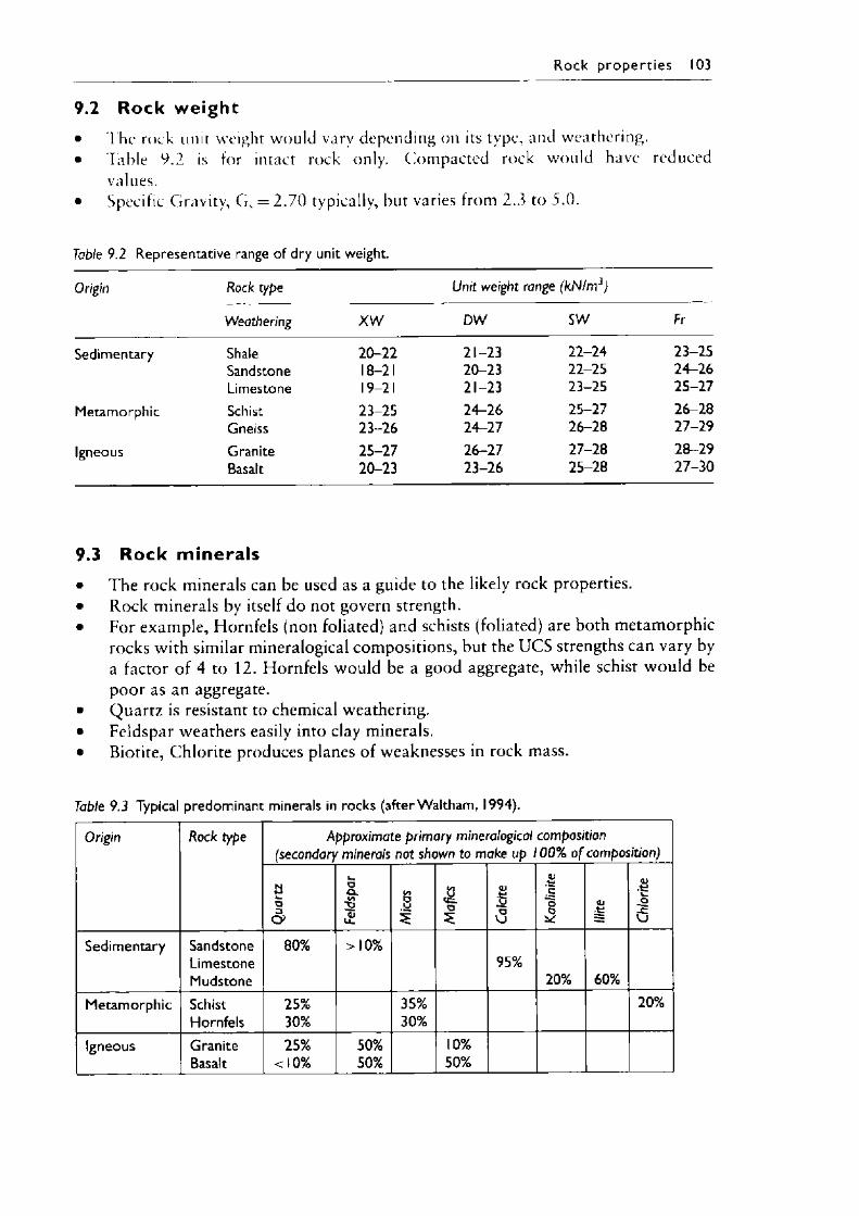
R o ck p ro p e r t ie s 103
9.2 Rock weight• The rock unit weight would vary depending on its type, and weathering.• Table 9.2 is for intact rock only. Compacted rock would have reduced
values.• Specific Gravity, G s = 2 .70 typically, but varies from 2.3 to 5.0.
Table 9.2 Representative range of dry unit weight.
Origin Rock type Unit weight range (kN/m3)
Weathering XW DW SW Fr
Sedimentary Shale 20-22 21-23 22-24 23-25Sandstone 18-21 20-23 22-25 24-26Limestone 19-21 21-23 23-25 25-27
Metamorphic Schist 23-25 24-26 25-27 26-28Gneiss 23-26 24-27 26-28 27-29
Igneous Granite 25-27 26-27 27-28 28-29Basalt 20-23 23-26 25-28 27-30
9.3 Rock minerals• The rock minerals can be used as a guide to the likely rock properties.• Rock minerals by itself do not govern strength.• For example, Hornfels (non foliated) and schists (foliated) are both metamorphic
rocks with similar mineralogical compositions, but the UCS strengths can vary by a factor of 4 to 12. Hornfels would be a good aggregate, while schist would be poor as an aggregate.
• Quartz is resistant to chemical weathering.• Feldspar weathers easily into clay minerals.• Biotite, Chlorite produces planes of weaknesses in rock mass.
Table 9.3 Typical predominant minerals in rocks (after Waltham, 1994).
Origin Rock type Approximate primary mineralogical composition (secondary minerals not shown to make up 100% o f composition)
Qua
rtz
Feld
spar <S)OU
it
toyjo
Calci
te
Kaol
inite
lllite
Chlo
rite
Sedimentary Sandstone 80% >10%Limestone 95%Mudstone 20% 60%
Metamorphic Schist 25% 35% 20%Hornfels 30% 30%
Igneous Granite 25% 50% 10%Basalt <10% 50% 50%
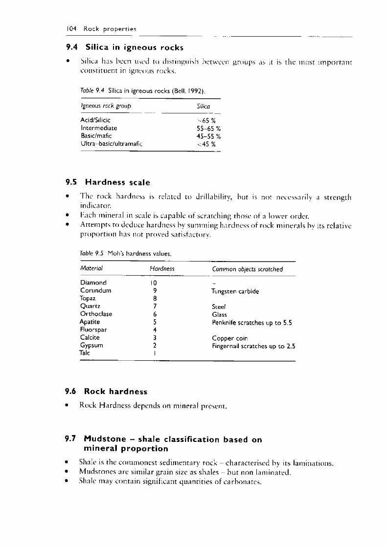
104 R o ck p ro p e r t ie s
9.4 Sil ica in igneous rocks• Silica has been used to distinguish between groups as it is the most important
constituent in igneous rocks.
Table 9.4 Silica in igneous rocks (Bell, 1992).
Igneous rock group Silica
Acid/Silicic >65 %Intermediate 55-65 %Basic/mafic 45-55 %Ultra-basic/ultramafic <45 %
9.5 Hardness scale• I he rock hardness is related to drillability, but is not necessarily a strength
indicator.• hach mineral in scale is capable of scratching those of a lower order.• Attempts to deduce hardness by summing hardness of rock minerals by its relative
proportion has not proved satisfactory.
Table 9.5 Moh’s hardness values.
Material Hardness Common objects scratched
Diamond 10 _Corundum 9 Tungsten carbideTopaz 8Quartz 7 SteelOrthoclase 6 GlassApatite 5 Penknife scratches up to 5.5Fluorspar 4Calcite 3 Copper coinGypsum 2 Fingernail scratches up to 2.5Talc 1
9.6 Rock hardness• Rock Hardness depends on mineral present.
9.7 Mudstone - shale classification based on mineral proportion
• Shale is the commonest sedimentary rock - characterised by its laminations.• Mudstones are similar grain size as shales - but non laminated.• Shale may contain significant quantities of carbonates.
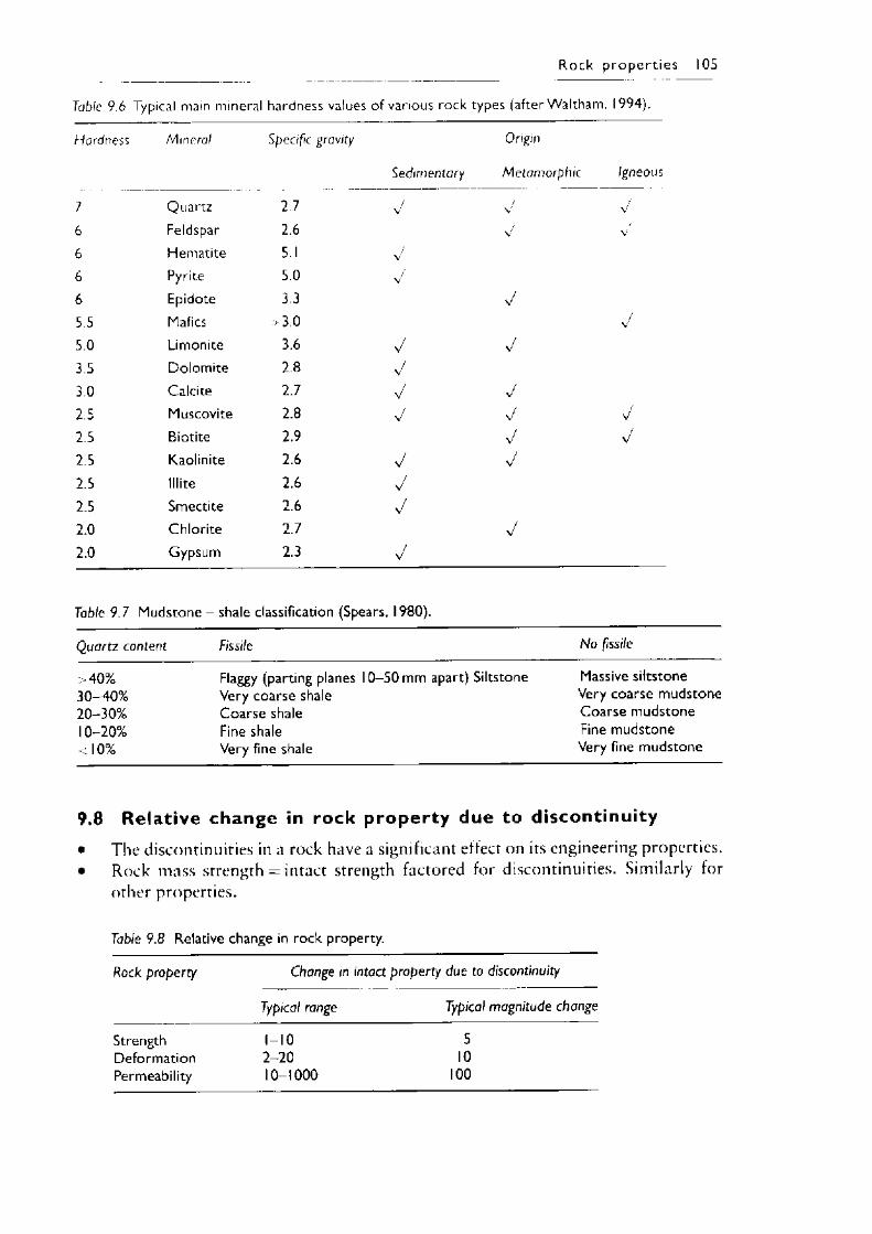
R o ck p ro p e rt ie s 105
Table 9.6 Typical main mineral hardness values of various rock types (after W altham, 1994).
Hardness Mineral Specific gravity Origin
Sedimentary Metamorphic Igneous
1 Quartz 2.7 V V V
6 Feldspar 2.6 V v
6 Hematite 5.1 V
6 Pyrite 5.0 >/6 Epidote 3.3 V5.5 Mafics >3.0 V
5.0 Limonite 3.6 V V3.5 Dolomite 2.8 v /
3.0 Calcite 2.7 V V 72.5 Muscovite 2.8 /V y y2.5 Biotite 2.9 y v2.5 Kaolinite 2.6 y v /
2.5 lllite 2.6 v /
2.5 Smectite 2.6 y2.0 Chlorite 2.7 y/2.0 Gypsum 2.3 y
Table 9.7 Mudstone - shale classification (Spears, 1980).
Quartz content Fissile No fissile
>40% Flaggy (parting planes 10-50 mm apart) Siltstone Massive siltstone30-40% Very coarse shale Very coarse mudstone20-30% Coarse shale Coarse mudstone10-20% Fine shale Fine mudstone<10% Very fine shale Very fine mudstone
9.8 Relative change in rock property due to discontinuity• The discontinuities in a rock have a significant effect on its engineering properties.• Rock mass strength = intact strength factored for discontinuities. Similarly for
other properties.
Table 9.8 Relative change in rock property.
Rock property Change in intact property due to discontinuity
Typical range Typical magnitude change
Strength 1-10 5Deformation 2-20 10Permeability 10-1000 100
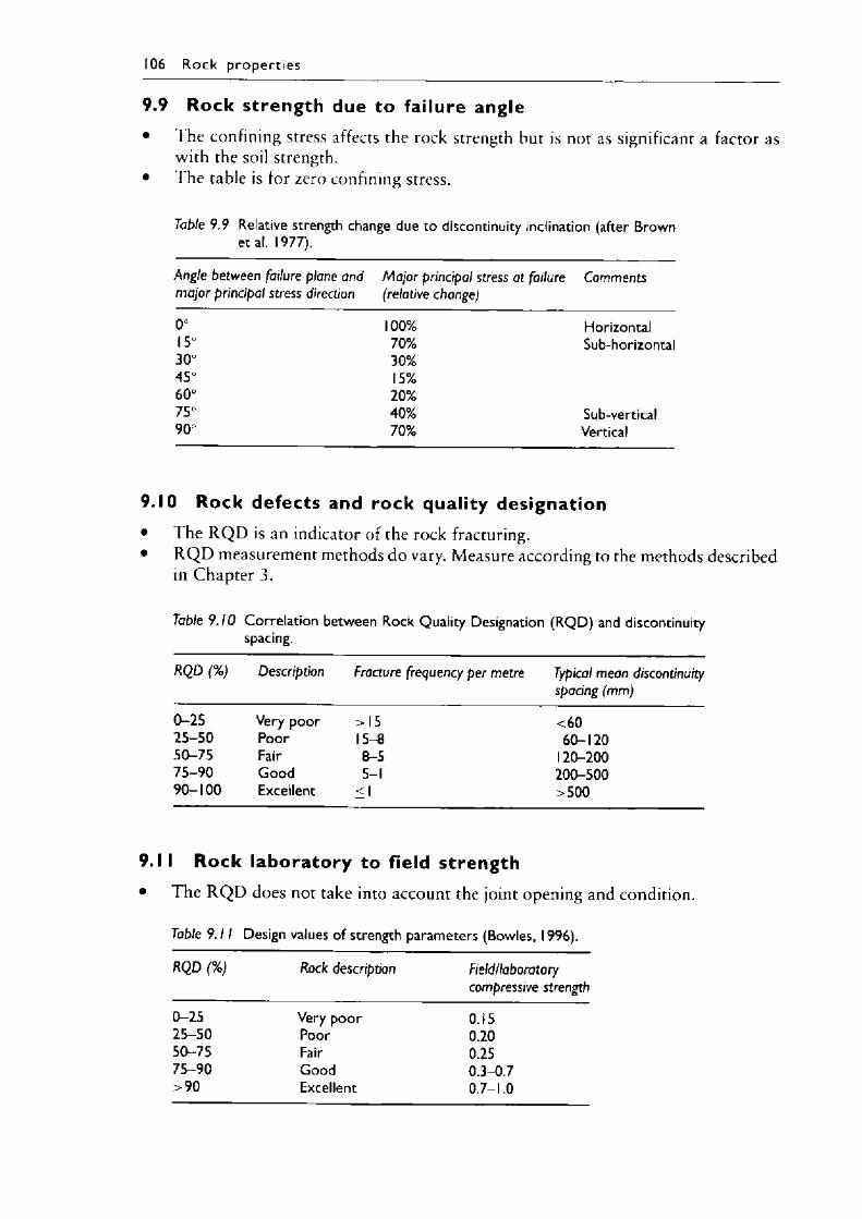
106 R o c k p ro p e r t ie s
9.9 Rock strength due to failure angle• The confining stress affects the rock strength but is not as significant a factor as
with the soil strength.• The table is for zero confining stress.
Table 9.9 Relative strength change due to discontinuity inclination (after Brown etal. 1977).
Angle between failure plane and major principal stress direction
M ajor principal stress at failure (relative change)
Comments
0° 100% Horizontal15° 70% Sub-horizontal30° 30%45° 15%60° 20%75° 40% Sub-vertical90 70% Vertical
9.10 Rock defects and rock quality designation• The R Q D is an indicator of the rock fracturing.• R Q D measurement methods do vary. Measure according to the methods described
in Chapter 3.
Table 9.10 Correlation between Rock Quality Designation (RQ D) and discontinuity spacing.
RQD (%) Description Fracture frequency per metre Typical mean discontinuity spacing (mm)
0-25 Very poor >15 <6025-50 Poor 15-8 60-12050-75 Fair 8-5 120-20075-90 Good 5-1 200-50090-100 Excellent <1 >500
9.11 Rock laboratory to field strength• The R Q D does not take into account the joint opening and condition.
Table 9 .11 Design values of strength parameters (Bowles, 1996).
RQD (%) Rock description Field/laboratory compressive strength
0-25 Very poor 0.1525-50 Poor 0.2050-75 Fair 0.2575-90 Good 0.3-0.7>90 Excellent 0.7-1.0
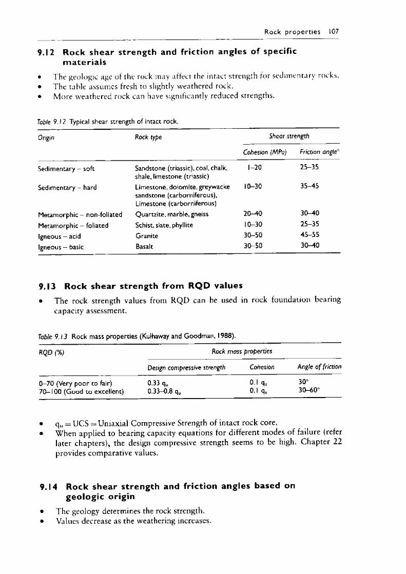
9.12 Rock shear strength and friction angles of specific m ater ia ls
• The geologic age of the rock may affect the intact strength for sedimentary rocks.• The table assumes fresh to slightly weathered rock.• More weathered rock can have significantly reduced strengths.
R o c k p ro p e r t ie s 107
Table 9.12 Typical shear strength of intact rock.
Origin Rock type Shear strength
Cohesion (MPa) Friction angle0
Sedimentary - soft Sandstone (triassic), coal, chalk, shale, limestone (triassic)
1-20 25-35
Sedimentary - hard Limestone, dolomite, greywacke sandstone (carborniferous), Limestone (carborniferous)
10-30 35-45
Metamorphic - non-foliated Quartzite, marble, gneiss 20—40 30-40Metamorphic - foliated Schist, slate, phyllite 10-30 25-35Igneous - acid Granite 30-50 45-55Igneous - basic Basalt 30-50 30-40
9.13 Rock shear strength from R Q D values• The rock strength values from R Q D can be used in rock foundation bearing
capacity assessment.
Table 9.13 Rock mass properties (Kulhaway and Goodman, 1988).
RQD (%) Rock mass properties
Design compressive strength Cohesion Angle o f friction
0-70 (Very poor to fair) 0.33 qu 0.1 qu 70-100 (Good to excellent) 0.33-0.8 qu 0.1 qy
30°30-60°
• q u = UCS = Uniaxial Compressive Strength of intact rock core.• When applied to bearing capacity equations for different modes of failure (refer
later chapters), the design compressive strength seems to be high. Chapter 22 provides comparative values.
9.14 Rock shear strength and friction angles based on geologic origin
• The geology determines the rock strength.• Values decrease as the weathering increases.
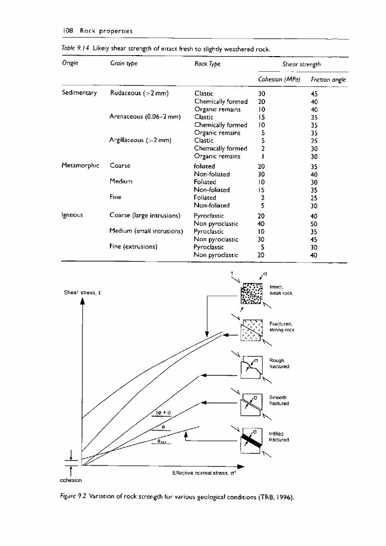
108 R ock p ro p e r t ie s
Table 9. 1 4 Likely shear strength of intact fresh to slightly weathered rock.
Origin Crain type Rock Type Shear strength
Cohesion (MPa) Friction angle
Igneous
Rudaceous (>2m m ) Clastic 30 45Chemically formed 20 40Organic remains 10 40
Arenaceous (0.06-2 mm) Clastic 15 35Chemically formed 10 35Organic remains 5 35
Argillaceous (>2m m ) Clastic 5 25Chemically formed 2 30Organic remains 1 30
Coarse foliated 20 35Non-foliated 30 40
Medium Foliated 10 30Non-foliated 15 35
Fine Foliated 2 25Non-foliated 5 30
Coarse (large intrusions) Pyroclastic 20 40Non pyroclastic 40 50
Medium (small intrusions) Pyroclastic 10 35Non pyroclastic 30 45
Fine (extrusions) Pyroclastic 5 30Non pyroclastic 20 40
Figure 9.2 Variation of rock strength for various geological conditions (TRB, 1996).
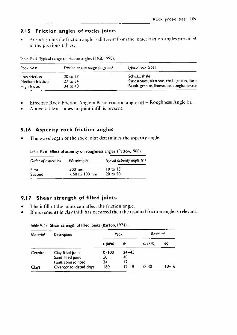
9.15 F r ic t io n angles of ro ck s joints• At rock joints the friction angle is different from the intact friction angles provided
in the previous tables.
R o c k p ro p e r t ie s 109
Table 9.15 Typical range of friction angles (TRB, 1990).
Rock class Friction angles range (degrees) Typical rock types
Low friction 20 to 27 Schists, shaleMedium friction 27 to 34 Sandstones, siltstone, chalk, gneiss, slateHigh friction 34 to 40 Basalt, granite, limestone, conglomerate
• Effective Rock Friction Angle = Basic Friction angle (<t>) + Roughness Angle (i).• Above table assumes no joint infill is present.
9.16 A s p e r i t y ro ck fr ic t ion angles• The wavelength of the rock joint determines the asperity angle.
Table 9 .16 Effect of asperity on roughness angles, (Patton, 1966).
Order o f asperities Wavelength Typical asperity angle (i°)
First 500 mm 10 to 15Second <50 to 100 mm 20 to 30
9.17 S h e a r strength of filled jo ints• The infill of the joints can affect the friction angle.• If movements in clay infill has occurred then the residual friction angle is relevant.
Table 9. 1 7 Shear strength of filled joints (Barton, 1974).
Material Description Peak Residual
c (kPa) <P° c r (kPa) <P°r
Granite Clay filled joint 0-100 24-45Sand-filled joint 50 40Fault zone jointed 24 42
Clays Overconsolidated clays 180 12-18 0-30 10-16
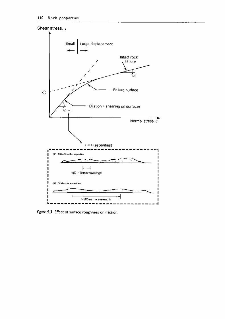
I 10 R o c k p ro p e r t ie s
Shear stress, x
(a ) Second-order asperities
<50-100 mm wavelength
(a ) First-order asperities
>500 mm wavelength
Figure 9.3 Effect of surface roughness on friction.
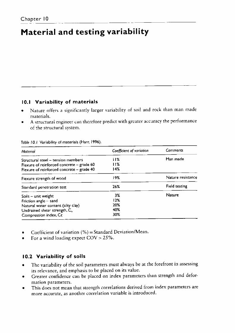
Ch apter 10
Material and testing variability
10.1 Variabi l i ty of m ater ia ls• Nature offers a significantly larger variability of soil and rock than man made
materials.• A structural engineer can therefore predict with greater accuracy the performance
of the structural system.
Table 1 0 .1 Variability of materials (Harr, 1996).
Material Coefficient o f variation Comments
Structural steel - tension members 1 1% Man madeFlexure of reinforced concrete - grade 60 1 1%Flexure of reinforced concrete - grade 40 14%
Flexure strength of wood 19% Nature resistance
Standard penetration test 26% Field testing
Soils - unit weight 3% NatureFriction angle - sand 12%Natural water content (silty clay) 20%Undrained shear strength, C u 40%Compression index, Cc 30%
• Coefficient of variation (% ) = Standard Deviation/Mean.• For a wind loading expect C O V > 2 5 % .
10.2 Var iab i l i ty of soils• The variability of the soil parameters must always be at the forefront in assessing
its relevance, and emphasis to be placed on its value.• Greater confidence can be placed on index parameters than strength and defor
mation parameters.• This does not mean that strength correlations derived from index parameters are
more accurate, as another correlation variable is introduced.
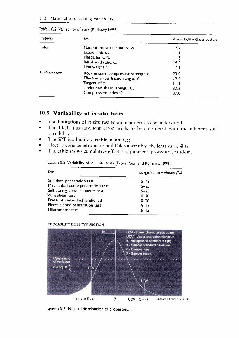
112 M a te r ia l and testing va r ia b i l i t y
Table 10.2 Variability of soils (Kulhawy, 1 992).
Property Test Mean COV without outliers
Index Natural moisture content, wn 17.7Liquid limit, LL 1 l.lPlastic limit, PL 1 1.3Initial void ratio, eQ 19.8Unit weight, y 7.1
Performance Rock uniaxial compressive strength, qu 23.0Effective stress friction angle, cf>' 12.6Tangent of ((>' 1 1.3Undrained shear strength C u 33.8Compression index C c 37.0
10.3 Var iabi l i ty of in-situ tests• The limitations of in-situ test equipment needs to be understood.• I he likely measurement error needs to be considered with the inherent soil
variability.• I he SPT is a highly variable in-situ test.• Electric cone penetrometer and Dilatometer has the least variability.• 1 he table shows cumulative effect of equipment, procedure, random.
Table 10.3 Variability of in - situ tests (From Poon and Kulhawy, 1999).
Test Coefficient o f variation (%)
Standard penetration test 15-45Mechanical come penetration test 15-25Self boring pressure meter test 15-25Vane shear test 10-20Pressure meter test, prebored 10-20Electric cone penetration test 5-15Dilatometer test 5-15
PROBABILITY DENSITY FUNCTION
LC V = X - kS X UCV = X + kS m e a s u re d p r o p e r t y v a lu e
Figure 10 .1 Normal distribution of properties.
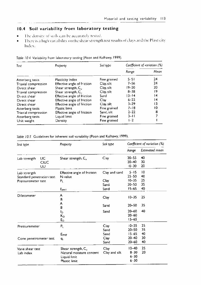
M ateria l and testing va r ia b i l i t y 113
10.4 Soi l v a r i a b i l i t y f r o m l a b o r a t o r y t es t i ng• The density of soils can he accurately tested.• There is a high variability on the shear strength test results of clays and the Plasticity
Index.
Table 10.4 Variability from laboratory testing (Poon and Kulhawy, 1999).
Test Property Soil type Coefficient o f variation (%)
Range Mean
Atterberg tests Plasticity index Fine grained 5-51 24Triaxial compression Effective angle of friction Clay, silt 7-56 24Direct shear Shear strength, C u Clay, silt 19-20 20Triaxial compression Shear strength, C u Clay, silt 8-38 19Dir ect shear Effective angle of friction Sand 13-14 14Direct shear Effective angle of friction Clay 6-22 14Direct shear Effective angle of friction Clay, silt 3-29 13Atterberg tests Plastic limit Fine grained 7-18 10Triaxial compression Effective angle of friction Sand, silt 2-22 8Atterberg tests Liquid limit Fine grained 3-1 1 7Unit weight Density Fine grained 1-2 1
Table 10.5 Guidelines for inherent soil variability (Poon and Kulhawy, 1999).
Test type Property Soil type Coefficient o f variation (%)
Range Estimated mean
Lab strength U C Shear strength, C u Clay 20-55 40C IU C 20—40 30UU 10-30 20
Lab strength Effective angle of friction Clay and sand 5-15 10Standard penetration test N-value 25-50 40Pressuremeter test P l Clay 10-35 25
Sand 20-50 35EpMT Sand 15-65 40
Dilatometer AB Clay 10-35 25
AB Sand 20-50 35
Id Sand 20-60 40K d 20-60E d 15-65
Pressuremeter P l Clay 10-35 25Sand 20-50 35
EpMT Sand 15-65 40Cone penetrometer test qc Clay 20—40 30
Sand 20-60 40
Vane shear test Lab index
Shear strength, C u Natural moisture content Liquid limit Plastic limit
ClayClay and silt
10-408-306-306-30
2520
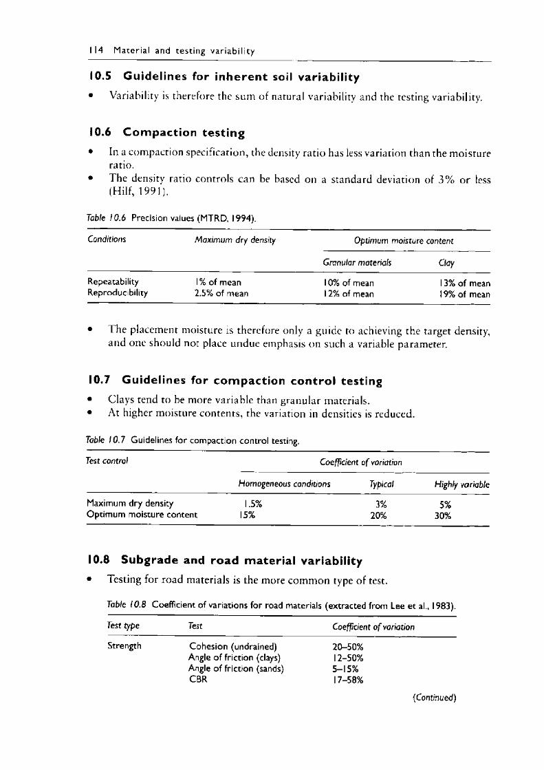
I 14 M ater ia l and testing va r ia b i l i t y
10.5 Guidelines for inherent soil variabil ity• Variability is therefore the sum of natural variability and the testing variability.
10.6 Com paction testing• In a compaction specification, the density ratio has less variation than the moisture
ratio.• The density ratio controls can be based on a standard deviation of 3 % or less
(Hilf, 1991).
Table 10.6 Precision values (MTRD, 1994).
Conditions Maximum dry density Optimum moisture content
Granular materials Clay
Repeatability 1% of mean 10% of mean 13% of meanReproducibility 2.5% of mean 12% of mean 19% of mean
• The placement moisture is therefore only a guide to achieving the target density, and one should not place undue emphasis on such a variable parameter.
10.7 Guidelines for compaction contro l testing• Clays tend to be more variable than granular materials.• At higher moisture contents, the variation in densities is reduced.
Table 10.7 Guidelines for compaction control testing.
Test control Coefficient o f variation
Homogeneous conditions Typical Highly variable
Maximum dry density 1.5% 3% 5%Optimum moisture content 15% 20% 30%
10.8 Subgrade and road material variabil ity• Testing for road materials is the more common type of test.
Table 10.8 Coefficient of variations for road materials (extracted from Lee et al., 1983).
Test type Test Coefficient o f variation
Strength Cohesion (undrained) 20-50%Angle of friction (clays) 12-50%Angle of friction (sands) 5-15%CBR 17-58%
(Continued)
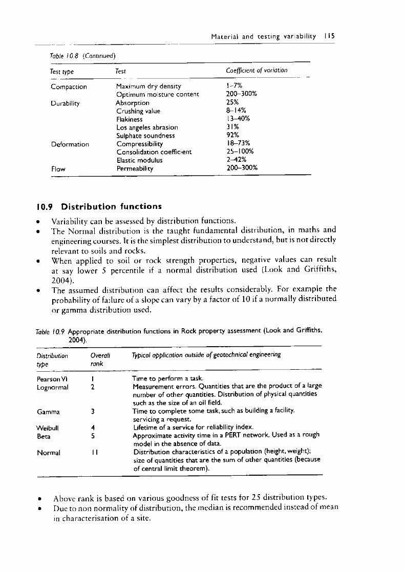
M ateria l and testing va r ia b i l i ty 115
Table 10.8 (Continued)
Test type Test Coefficient o f variation
Compaction Maximum dry density 1-7%Optimum moisture content 200-300%
Durability Absorption 25%Crushing value 8-14%Flakiness 13—40%Los angeles abrasion 31%Sulphate soundness 92%
Deformation Compressibility 18-73%Consolidation coefficient 25-100%Elastic modulus 2-42%
Flow Permeability 200-300%
10.9 Distribution functions• Variability can be assessed by distribution functions.• The Normal distribution is the taught fundamental distribution, in maths and
engineering courses. It is the simplest distribution to understand, but is not directly relevant to soils and rocks.
• When applied to soil or rock strength properties, negative values can result at say lower 5 percentile if a normal distribution used (Look and Griffiths, 2004) .
• The assumed distribution can affect the results considerably. For example the probability of failure of a slope can vary by a factor of 10 if a normally distributed or gamma distribution used.
Table 10.9 Appropriate distribution functions in Rock property assessment (Look and Griffiths, 2004).
Distribution Overall Typical application outside o f geotechnical engineeringtype rank
Pearson VI 1 Time to perform a task.Lognormal 2 Measurement errors. Quantities that are the product of a large
number of other quantities. Distribution of physical quantities such as the size of an oil field.
Gamma 3 Time to complete some task, such as building a facility, servicing a request.
Weibull 4 Lifetime of a service for reliability index.Beta 5 Approximate activity time in a PERT network. Used as a rough
model in the absence of data.Normal 11 Distribution characteristics of a population (height, weight);
size of quantities that are the sum of other quantities (because of central limit theorem).
• Above rank is based on various goodness of fit tests for 25 distribution types.• Due to non normality of distribution, the median is recommended instead of mean
in characterisation of a site.
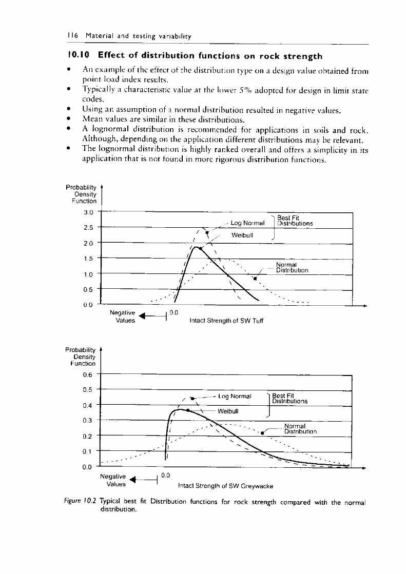
116 M ate r ia l and test ing va r iab i l i ty
10.10 Effect of distribution functions on rock strength• An example of the effect of the distribution type on a design value obtained from
point load index results.• Typically a characteristic value at the lower 5 % adopted for design in limit state
codes.• Using an assumption of a normal distribution resulted in negative values.• Mean values are similar in these distributions.• A lognormal distribution is recommended for applications in soils and rock.
Although, depending on the application different distributions may be relevant.• The lognormal distribution is highly ranked overall and offers a simplicity in its
application that is not found in more rigorous distribution functions.
Negative ^ ________ i 0 0Values Intact Strength of SW Greywacke
Figure 10.2 Typical best fit Distribution functions for rock strength compared with the normal distribution.
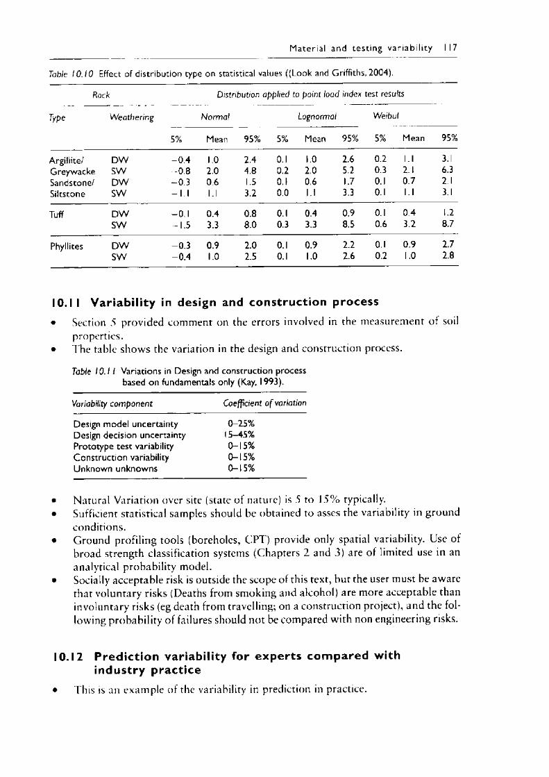
M ateria l and testing v a r ia b i l i t y 117
Table 10.10 Effect of distribution type on statistical values ((Look and Griffiths, 2004).
Rock Distribution applied to point load index test results
Type Weathering Normal Lognormal Weibul
5% Mean 95% 5% Mean 95% 5% Mean 95%
Argillite/ D W 0.4 1.0 2.4 0.1 1.0 2.6 0.2 l.l 3.1Greywacke SW 0.8 2.0 4.8 0.2 2.0 5.2 0.3 2.1 6.3Sandstone/ D W -0 .3 0.6 1.5 0.1 0.6 1.7 0.1 0.7 2.1Siltstone SW - l . l l.l 3.2 0.0 l.l 3.3 0.1 l.l 3.1
Tuff D W -0.1 0.4 0.8 0.1 0.4 0.9 0.1 0.4 1.2SW -1 .5 3.3 8.0 0.3 3.3 8.5 0.6 3.2 8.7
Phyllites D W -0 .3 0.9 2.0 0.1 0.9 2.2 0.1 0.9 2.7SW -0 .4 1.0 2.5 0.1 1.0 2.6 0.2 1.0 2.8
10.11 Var iabi l i ty in design and construction process• Section 5 provided comment on the errors involved in the measurement o f soil
properties.• The table shows the variation in the design and construction process.
Table 10.1 I Variations in Design and construction process based on fundamentals only (Kay, 1993).
Variability component Coefficient o f variation
Design model uncertainty 0-25%Design decision uncertainty 15—45%Prototype test variability 0-15%Construction variability 0-15%Unknown unknowns 0-15%
• Natural Variation over site (state of nature) is 5 to 1 5 % typically.• Sufficient statistical samples should be obtained to asses the variability in ground
conditions.• Ground profiling tools (boreholes, CPT) provide only spatial variability. Use of
broad strength classification systems (Chapters 2 and 3) are of limited use in an analytical probability model.
• Socially acceptable risk is outside the scope of this text, but the user must be aware that voluntary risks (Deaths from smoking and alcohol) are more acceptable than involuntary risks (eg death from travelling; on a construction project), and the following probability of failures should not be compared with non engineering risks.
10.12 Predict ion variabil ity for experts com pared with industry practice
• This is an example of the variability in prediction in practice.
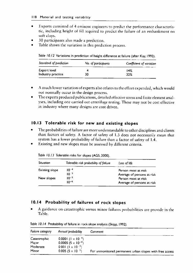
I 18 M ate r ia l and test ing va r iab i l i ty
• Experts consisted of 4 eminent engineers to predict the performance characteristic, including height of fill required to predict the failure o f an embankment on soft clays.
• 3 0 participants also made a prediction.• Table shows the variation in this prediction process.
Table 10.12 Variations in prediction of height difference at failure (after Kay, 1993).
Standard o f prediction No. o f participants Coefficient o f variation
Expert level 4 14%Industry practice 30 32%
• A much lower variation of experts also relates to the effort expended, which would not normally occur in the design process.
• The experts produced publications, detailed effective stress and finite element analyses, including one carried out centrifuge testing. These may not be cost effective in industry where many designs are cost driven.
10.13 T o le rab le risk for new and existing slopes• 1 he probabilities of failure are more understandable to other disciplines and clients
than factors of safety. A factor of safety of 1.3 does not necessarily mean thatsystem has a lower probability of failure than a factor of safety of 1.4.
• Existing and new slopes must be assessed by different criteria.
Table 10.13 Tolerable risks for slopes (AGS, 2000).
Situation Tolerable risk probability o f failure Loss o f life
Existing slope 10 4 Person most at risk10 5 Average of persons at risk
New slopes 10 5 Person most at risk10 6 Average of persons at risk
10.14 Probabil ity of failures of rock slopes• A guidance on catastrophic v<?rsus minor failures probabilities are provide in the
Table.
Table 10.14 Probability of failure in rock slope analysis (Skipp, 1992).
Failure category Annual probability Comment
Catastrophic 0.0001 (1 x 10 4)Major 0.0005 (5 x 10 4)Moderate 0001 (1 x 10 3)Minor 0.005 (5 x 10 3) For unmonitored permanent urban slopes with free access
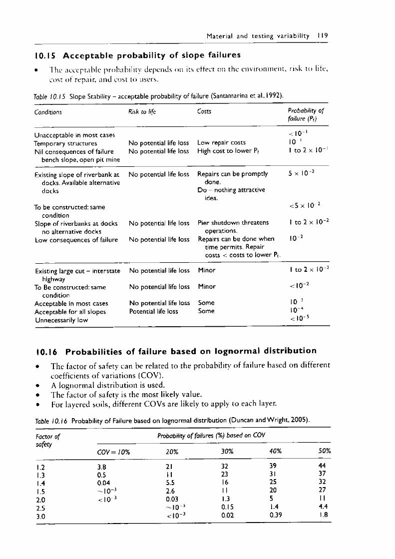
M ateria l and testing v a r ia b i l i t y 119
10.15 A ccep tab le probability of slope failures• The acceptable probability depends on its effect on the environment, risk to life,
cost of repair, and cost to users.
Table 10.15 Slope Stability - acceptable probability of failure (Santamarina et al., 1992).
Conditions Risk to life Costs Probability o f failure ( Pf )
Unacceptable in most cases < 10“ 'Temporary structures No potential life loss Low repair costs 10 1Nil consequences of failure No potential life loss High cost to lower Pf 1 to 2 X 10 1
bench slope, open pit mine
Existing slope of riverbank at docks. Available alternative docks
To be constructed: same
No potential life loss Repairs can be promptly done.
Do - nothing attractive idea.
5 x 10 2
<5 x 10 2condition
Slope of riverbanks at docks no alternative docks
No potential life loss Pier shutdown threatens operations.
1 to 2 x 10 z
Low consequences of failure No potential life loss Repairs can be done when time permits. Repair costs < costs to lower Pf.
10 2
Existing large cut - interstate No potential life loss Minor 1 to 2 x 10 2highway
To Be constructed: same No potential life loss Minor <10 zcondition
Acceptable in most cases No potential life loss Some 10 jAcceptable for all slopes Unnecessarily low
Potential life loss Some 10 4 <10 5
10.16 Probabil it ies of failure based on lognormal distr ibution• The factor of safety can be related to the probability of failure based on different
coefficients of variations (COV).• A lognormal distribution is used.• The factor o f safety is the most likely value.• For layered soils, different C O Vs are likely to apply to each layer.
Table 10.16 Probability of Failure based on lognormal distribution (Duncan and Wright, 2005).
Factor o f Probability o f failures (%) based on COVsafety —----------------------------------------
COV = 1 0 % 20% 30% 40% 50%
1.2 3.8 21 32 39 441.3 0.5 1 1 23 31 371.4 0.04 5.5 16 25 321.5 - 1 0 3 2.6 1 1 20 272.0 <10 3 0.03 1.3 5 1 12.5 - 1 0 3 0.15 1.4 4.43.0 <10 3 0.02 0.39 1.8
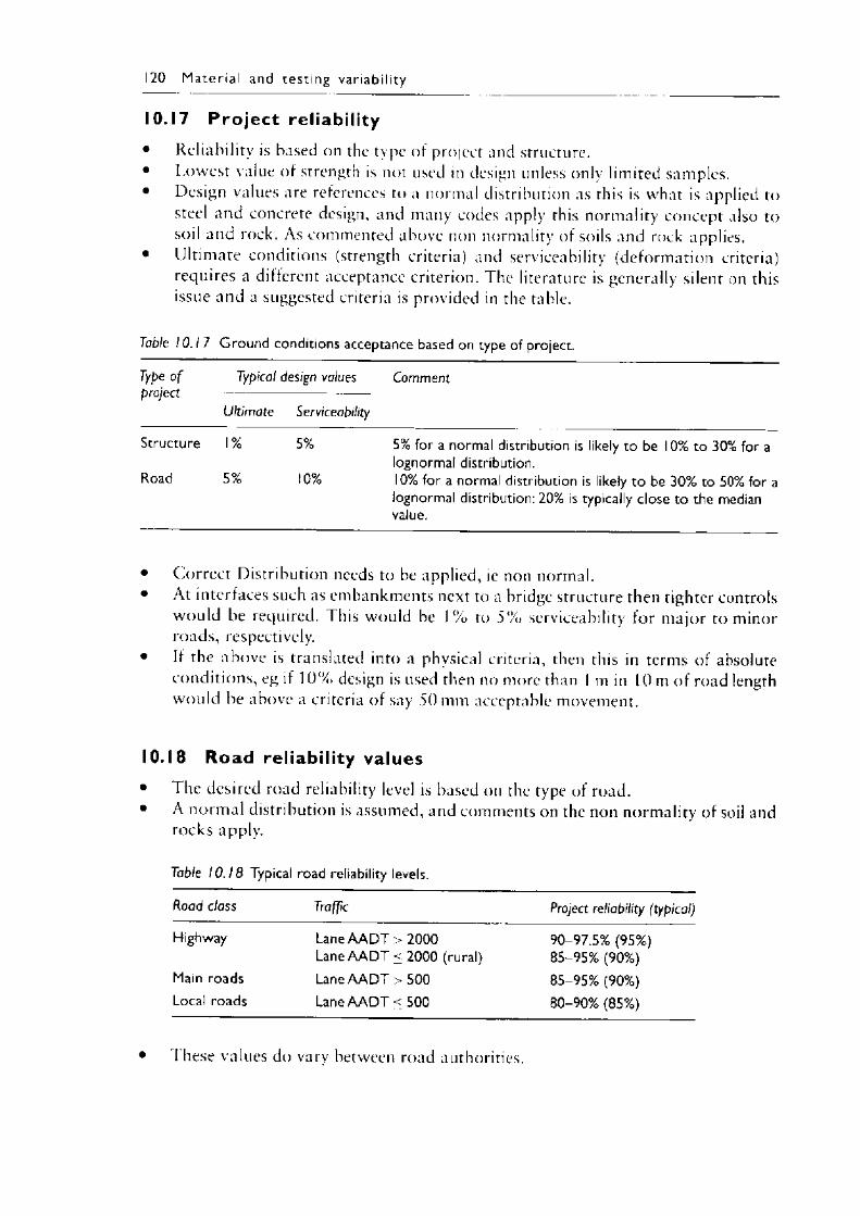
10.17 Pro ject reliability• Reliability is based on the type of project and structure.• Lowest value of strength is not used in design unless only limited samples.• Design values are references to a normal distribution as this is what is applied to
steel and concrete design, and many codes apply this normality concept also tosoil and rock. As commented above non normality of soils and rock applies.
• Ultimate conditions (strength criteria) and serviceability (deformation criteria) requires a different acceptance criterion. The literature is generally silent on this issue and a suggested criteria is provided in the table.
120 M ate r ia l and test ing va r iab i l i ty
Table 10.1 7 Ground conditions acceptance based on type of project.
Type o f project
Typical design values
Ultimate Serviceability
Comment
Structure 1 % 5% 5% for a normal distribution is likely to be 10% to 30% for a lognormal distribution.
Road 5% 10% 10% for a normal distribution is likely to be 30% to 50% for a lognormal distribution: 20% is typically close to the median value.
• Correct Distribution needs to be applied, ie non normal.• At interfaces such as embankments next to a bridge structure then tighter controls
would be required. I his would be 1% to 5 % serviceability for major to minor roads, respectively.
• If the above is translated into a physical criteria, then this in terms of absolute conditions, eg if 1 0 % design is used then no more than I m in 1 0 m of road length would be above a criteria of say 50 mm acceptable movement.
10.18 Road reliabil ity values• The desired road reliability level is based on the type of road.• A normal distribution is assumed, and comments on the non normality of soil and
rocks apply.
Table 10.18 Typical road reliability levels.
Road class Traffic Project reliability (typical)
Highway LaneA A D T > 2000 90-97.5% (95%)Lane A A D T < 2000 (rural) 85-95% (90%)
Main roads LaneA AD T > 500 85-95% (90%)Local roads Lane A A D T < 500 80-90% (85%)
These values do vary between road authorities.
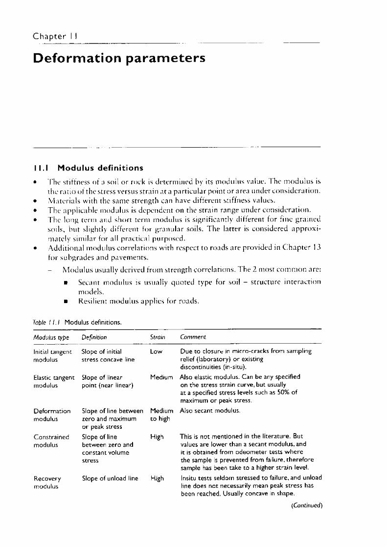
Chapter i I
Deform ation param eters
I 1.1 Modulus definitions• The stiffness of a soil or rock is determined by its modulus value. 1 he modulus is
the ratio of the stress versus strain at a particular point or area under consideration.• Materials with the same strength can have different stiffness values.• The applicable modulus is dependent on the strain range under consideration.• The long term and short term modulus is significantly different for fine grained
soils, but slightly different for granular soils. The latter is considered approximately similar tor all practical purposed.
• Additional modulus correlations with respect to roads are provided in Chapter 13 for subgrades and pavements.
Modulus usually derived from strength correlations. The 2 most common are:
■ Secant modulus is usually quoted type for soil - structure interaction models.
■ Resilient modulus applies for roads.
Table 11.1 Modulus definitions.
Modulus type Definition Strain Comment
Initial tangent modulus
Elastic tangent modulus
Deformationmodulus
Constrainedmodulus
Recoverymodulus
Slope of initial Lowstress concave line
Slope of linear Mediumpoint (near linear)
Slope of line between Mediumzero and maximum to highor peak stressSlope of line Highbetween zero and constant volume stress
Slope of unload line High
Due to closure in micro-cracks from sampling relief (laboratory) or existing discontinuities (in-situ).Also elastic modulus. Can be any specified on the stress strain curve, but usually at a specified stress levels such as 50% of maximum or peak stress.Also secant modulus.
This is not mentioned in the literature. But values are lower than a secant modulus, and it is obtained from odeometer tests where the sample is prevented from failure, therefore sample has been take to a higher strain level.Insitu tests seldom stressed to failure, and unload line does not necessarily mean peak stress has been reached. Usually concave in shape.
(Continued)
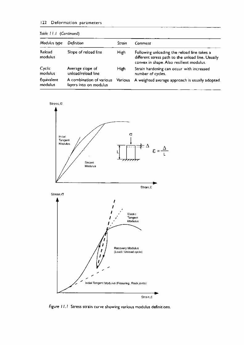
122 D e fo rm a t io n p aram ete rs
Table I 1.1 (Continued)
Modulus type Definition Strain Comment
Reloadmodulus
Slope of reload line High Following unloading the reload line takes a different stress path to the unload line. Usually convex in shape. Also resilient modulus.
Cyclicmodulus
Average slope of unload/reload line
High Strain hardening can occur with increased number of cycles.
Equivalentmodulus
A combination of various layers into on modulus
Various A weighted average approach is usually adopted.
Stress. (T
S tress.a
Figure 11.1 Stress strain curve showing various modulus definitions.
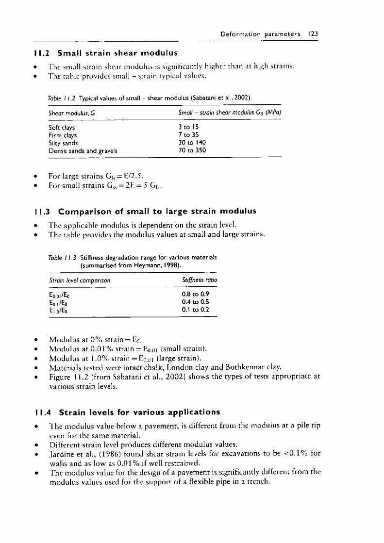
D e fo rm a t io n p a ra m e te rs 123
11.2 Small strain shear modulus• The small strain shear modulus is significantly higher than at high strains.• The table provides small - strain typical values.
Table 11.2 Typical values of small - shear modulus (Sabatani et al., 2002).
Shear modulus, G Small - strain shear modulus G0 (MPa)
Soft clays 3 to 15Firm clays 7 to 35Silty sands 30 to 140Dense sands and gravels 70 to 350
• For large strains Gjs = E/2.5.• For small strains G ss = 2E = 5 G|s.
I 1.3 C o m p ar iso n of small to large strain modulus• The applicable modulus is dependent on the strain level.• The table provides the modulus values at small and large strains.
Table 11.3 Stiffness degradation range for various materials (summarised from Heymann, 1998).
Strain level comparison Stiffness ratio
Eooi/Eq 0.8 to 0.9
oLUoLU 0.4 to 0.5
oLUoLU 0.1 to 0.2
• Modulus at 0 % strain = Eo.• Modulus at 0.01 % strain = Eo.oi (small strain).• Modulus at 1 .0 % strain = Eo.oi (large strain).• Materials tested were intact chalk, London clay and Bothkennar clay.• Figure 11.2 (from Sabatani et al., 2 0 0 2 ) shows the types of tests appropriate at
various strain levels.
11.4 Stra in levels for various applications• The modulus value below a pavement, is different from the modulus at a pile tip
even for the same material.• Different strain level produces different modulus values.• Jardine et al., (1986) found shear strain levels for excavations to be < 0 . 1 % for
walls and as low as 0.01 % if well restrained.• The modulus value for the design of a pavement is significantly different from the
modulus values used for the support o f a flexible pipe in a trench.
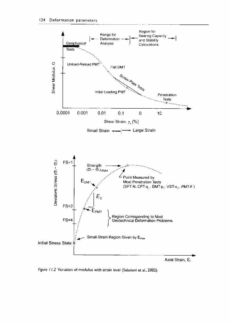
124 D e fo rm a t io n param ete rs
Shear Strain, v s (% )
Small Strain — I— — Large Strain
b
c/5</)Q)t _
COoo•
>0)o
FS=1
FS=2
FS=4
Initial Stress State
Strength —( Oi - Oi)m ax
■DMT
7Point Measured byMost Penetration Tests(SPT-N, CPT-qc , DMT-p,, VST-suv, PMT-F )
•PMT
Region Corresponding to Most Geotechnical Deformation Problems
Small-Strain Region Given by E r
Axial Strain, £
Figure 11.2 Variation of modulus with strain level (Sabatani et al.,2002).
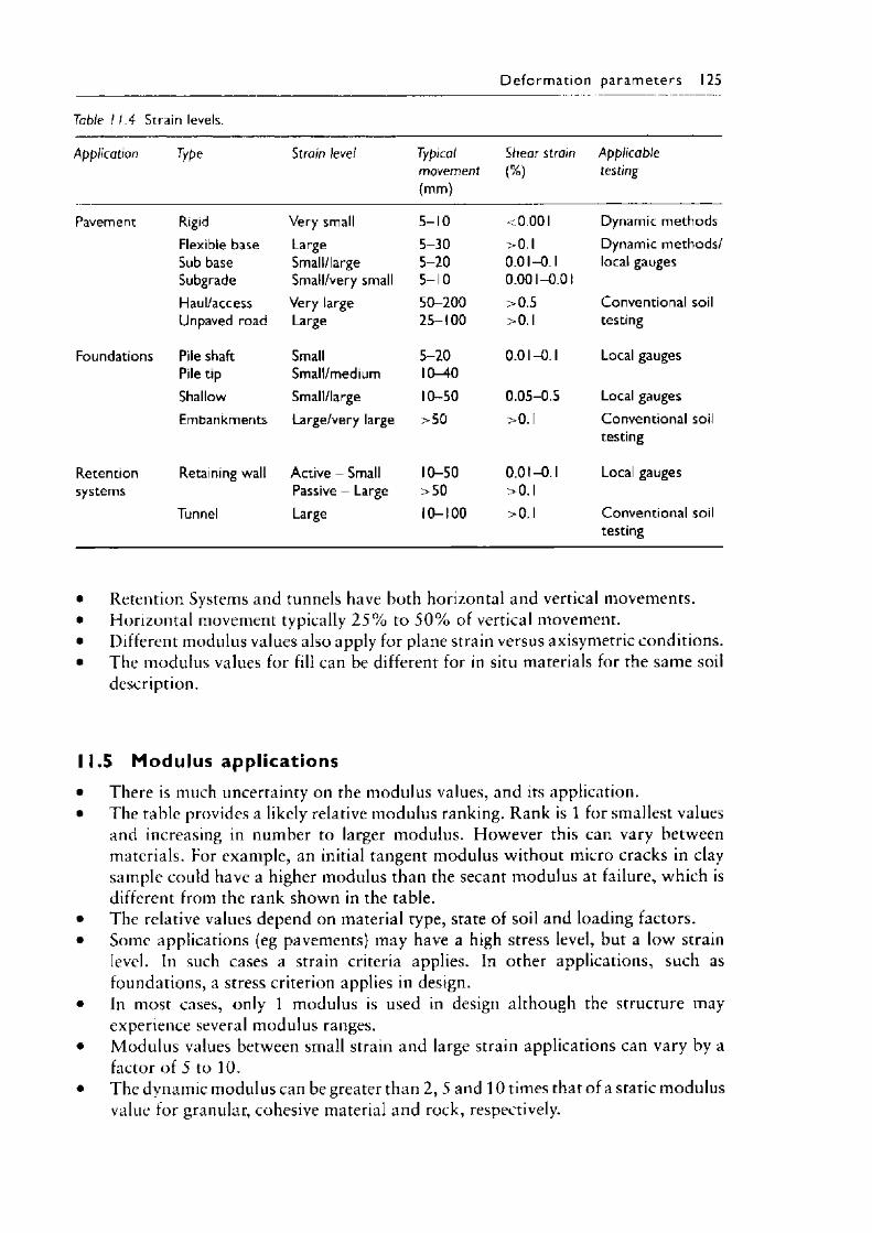
D e fo rm a t io n p a ra m e te rs 125
Table I 1.4 Strain levels.
Application Type Strain level Typicalmovement(mm)
Shear strain (%)
Applicabletesting
Pavement Rigid Very small 5-10 <0.001 Dynamic methodsFlexible base Large 5-30 >0.1 Dynamic methods/Sub base Small/large 5-20 0.01-0.1 local gaugesSubgrade Small/very small 5-10 0.001-0.01Haul/access Very large 50-200 >0.5 Conventional soilUnpaved road Large 25-100 >0.1 testing
Foundations Pile shaft Small 5-20 0.01-0.1 Local gaugesPile tip Small/medium 10-40Shallow Small/large 10-50 0.05-0.5 Local gaugesEmbankments Large/very large >50 >0.1 Conventional soil
testing
Retention Retaining wall Active - Small 10-50 0.01-0.1 Local gaugessystems Passive - Large >50 >0.1
Tunnel Large 10-100 >0.1 Conventional soiltesting
• Retention Systems and tunnels have both horizontal and vertical movements.• Horizontal movement typically 2 5 % to 5 0 % of vertical movement.• Different modulus values also apply for plane strain versus axisymetric conditions.• The modulus values for fill can be different for in situ materials for the same soil
description.
I 1.5 Modulus applications• There is much uncertainty on the modulus values, and its application.• The table provides a likely relative modulus ranking. Rank is 1 for smallest values
and increasing in number to larger modulus. However this can vary between materials. For example, an initial tangent modulus without micro cracks in clay sample could have a higher modulus than the secant modulus at failure, which is different from the rank shown in the table.
• The relative values depend on material type, state of soil and loading factors.• Some applications (eg pavements) may have a high stress level, but a low strain
level. In such cases a strain criteria applies. In other applications, such as foundations, a stress criterion applies in design.
• In most cases, only 1 modulus is used in design although the structure may experience several modulus ranges.
• Modulus values between small strain and large strain applications can vary by a factor of 5 to 10.
• The dynamic modulus can be greater than 2, 5 and 10 times that of a static modulus value for granular, cohesive material and rock, respectively.
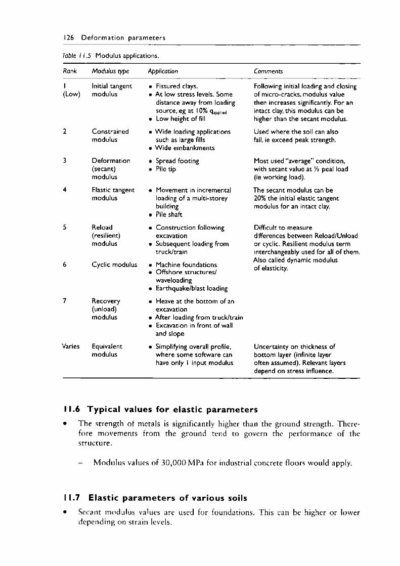
126 D e fo rm a t io n p a ra m e te rs
Table 11.5 Modulus applications.
Rank Modulus type Application Comments
1 Initial tangent • Fissured clays. Following initial loading and closing(Low) modulus • At low stress levels. Some
distance away from loading source, eg at 10% qappi(ed
• Low height of fill
of micro-cracks, modulus value then increases significantly. For an intact clay, this modulus can be higher than the secant modulus.
2 Constrained • W ide loading applications Used where the soil can alsomodulus such as large fills
• W ide embankmentsfail, ie exceed peak strength.
3 Deformation • Spread footing Most used “average” condition,(secant)modulus
• Pile tip with secant value at Vi peal load (ie working load).
4 Elastic tangent • Movement in incremental The secant modulus can bemodulus loading of a multi-storey
building • Pile shaft
20% the initial elastic tangent modulus for an intact clay.
5 Reload • Construction following Difficult to measure(resilient) excavation differences between Reload/Unloadmodulus • Subsequent loading from
truck/trainor cyclic. Resilient modulus term interchangeably used for all of them. Also called dynamic modulus6 Cyclic modulus • Machine foundations
• Offshore structures/ waveloading
• Earthquake/blast loading
of elasticity.
7 Recovery(unload)modulus
• Heave at the bottom of an excavation
• After loading from truck/train• Excavation in front of wall
and slope
Varies Equivalent • Simplifying overall profile, Uncertainty on thickness ofmodulus where some software can
have only 1 input modulusbottom layer (infinite layer often assumed). Relevant layers depend on stress influence.
11.6 Typ ica l values for elastic param eters• The strength of metals is significantly higher than the ground strength. There
fore movements from the ground tend to govern the performance of the structure.
- Modulus values of 3 0 , 0 0 0 MPa for industrial concrete floors would apply.
11.7 E last ic p ara m e te rs of various soils• Secant modulus values are used for foundations. This can be higher or lower
depending on strain levels.
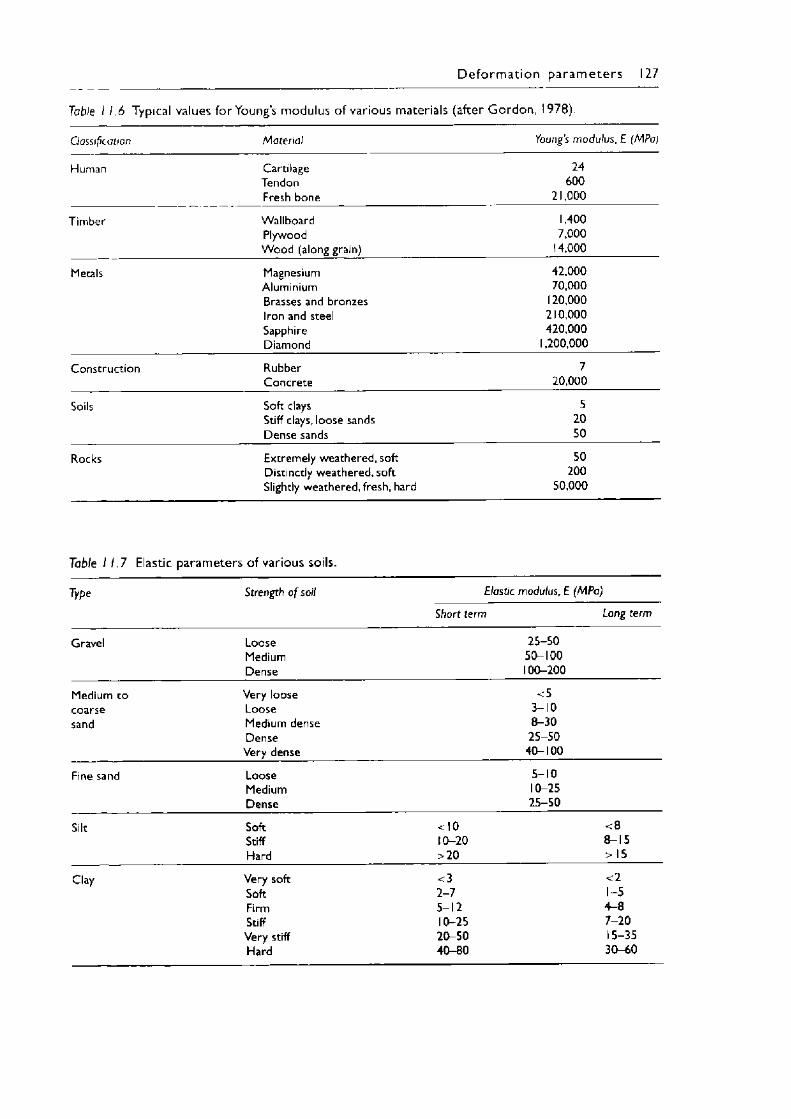
D e fo rm a t io n p a ra m e te r s 127
Table 1 1.6 Typical vallues for Young’s modulus of various materials (after Gordon, 1978).
Classification Material Young's modulus, E (MPa)
Human Cartilage 24Tendon 600Fresh bone 21,000
Timber Wallboard 1,400Plywood 7,000Wood (along grain) 14,000
Metals Magnesium 42,000Aluminium 70,000Brasses and bronzes 120,000Iron and steel 210,000Sapphire 420,000Diamond 1,200,000
Construction Rubber 7Concrete 20,000
Soils Soft clays 5Stiff clays, loose sands 20Dense sands 50
Rocks Extremely weathered, soft 50Distinctly weathered, soft 200Slightly weathered, fresh, hard 50,000
Table 1 1.7 Elastic parameters of various soils.
Type Strength of soil Elastic modulus, E (MPa)
Short term Long term
Gravel Loose 25-50Medium 50-100Dense 100-200
Medium to Very loose <5coarse Loose 3-10sand Medium dense 8-30
Dense 25-50Very dense 40-100
Fine sand Loose 5-10Medium 10-25Dense 25-50
Silt Soft <10 <8Stiff 10-20 8-15Hard >20 >15
Clay Very soft <3 <2Soft 2-7 1-5Firm 5-12 4-8Stiff 10-25 7-20Very stiff 20-50 15-35Hard 40-80 30-60
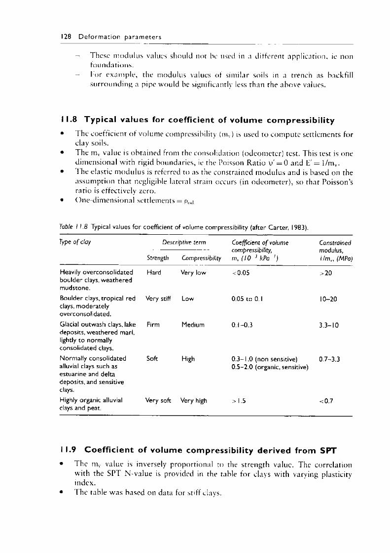
128 D e fo rm a t io n p a ra m e te rs
I hesc modulus values should not he used in a different application, ie non foundations.
- For example, the modulus values of similar soils in a trench as backfill surrounding a pipe would be significantly less than the above values.
I 1.8 Typ ica l values for coefficient of vo lume compress ib i l i ty• I he coefficient o f volume compressibility (mv) is used to compute settlements for
clay soils.• The m v value is obtained from the consolidation (odeometer) test. This test is one
dimensional with rigid boundaries, ie the Poisson Ratio v' = 0 and E' = l/mv.• The elastic modulus is referred to as the constrained modulus and is based on the
assumption that negligible lateral strain occurs (in odeometer), so that Poisson’s ratio is effectively zero.
• One-dimensional settlements = p()(j
Table 11.8 Typical values for coefficient of volume compressibility (after Carter, 1983).
Type o f clay Descriptive term
Strength Compressibility
Coefficient o f volume compressibility, mv (10 3 kPa ')
Constrained modulus, l/m v, (MPa)
Heavily overconsolidated boulder clays, weathered mudstone.
Hard Very low <0.05 >20
Boulder clays, tropical red clays, moderately overconsolidated.
Very stiff Low 0.05 to 0.1 10-20
Glacial outwash clays, lake deposits, weathered marl, lightly to normally consolidated clays.
Firm Medium p p OJ 3.3-10
Normally consolidated alluvial clays such as estuarine and delta deposits, and sensitive clays.
Soft High 0.3-1.0 (non sensitive)0.5-2.0 (organic, sensitive)
0.7-3.3
Highly organic alluvial clays and peat.
Very soft Very high >1.5 <0.7
11.9 Coeff ic ien t of volume compressib i l i ty derived from SPT• The mv value is inversely proportional to the strength value. The correlation
with the SP1 N-value is provided in the table for clays with varying plasticity index.
• The table was based on data for stiff clays.
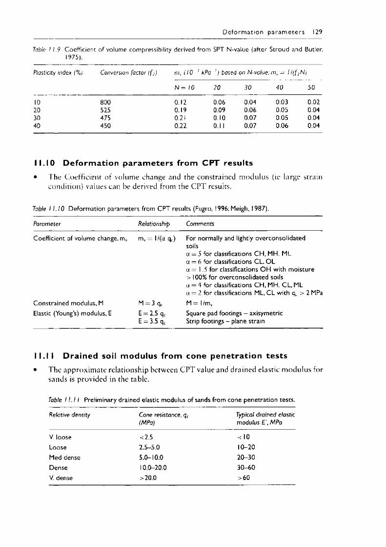
D e fo rm a t io n p a r a m e te r s 129
Table I 1.9 Coefficient of volume compressibility derived from SPT N-value (after Stroud and Butler, 1975).
Plasticity index (%) Conversion factor ( f2) mv (10 ? kPa 1) based on N-value: mv = l/ ( f2N)
N = 10 20 30 40 50
10 800 0.12 0.06 0.04 0.03 0.0220 525 0.19 0.09 0.06 0.05 0.0430 475 0.21 0.10 0.07 0.05 0.0440 450 0.22 0.1 1 0.07 0.06 0.04
11.10 Deform ation p aram eters from C P T results• The Coefficient of volume change and the constrained modulus (ie large strain
condition) values can be derived from the CPT results.
Table 11.10 Deformation parameters from C P T results (Fugro, l996;Meigh, 1987).
Parameter Relationship Comments
Coefficient of volume change, mv mv = l/(a qc) For normally and lightly overconsolidated soilsoi = 5 for classifications C H , MH. MLa = 6 for classifications C L , O La = 1.5 for classifications O H with moisture> 100% for overconsolidated soilsa = 4 for classifications C H , MH. C L , MLa = 2 for classifications ML, C L with qc > 2 MPa
Constrained modulus, M M = 3 q c M = l/mvElastic (Young’s) modulus, E E = 2.5 qc
E = 3.5 qcSquare pad footings - axisymetric Strip footings - plane strain
11.11 Dra ined soil modulus from cone penetrat ion tests• The approximate relationship between C P T value and drained elastic modulus for
sands is provided in the table.
Table 11.11 Preliminary drained elastic modulus of sands from cone penetration tests.
Relative density Cone resistance, qc (MPa)
Typical drained elastic modulus £', MPa
V. loose <2.5 <10Loose 2.5-5.0 10-20Med dense 5.0-10.0 20-30Dense 10.0-20.0 30-60V. dense >20.0 >60
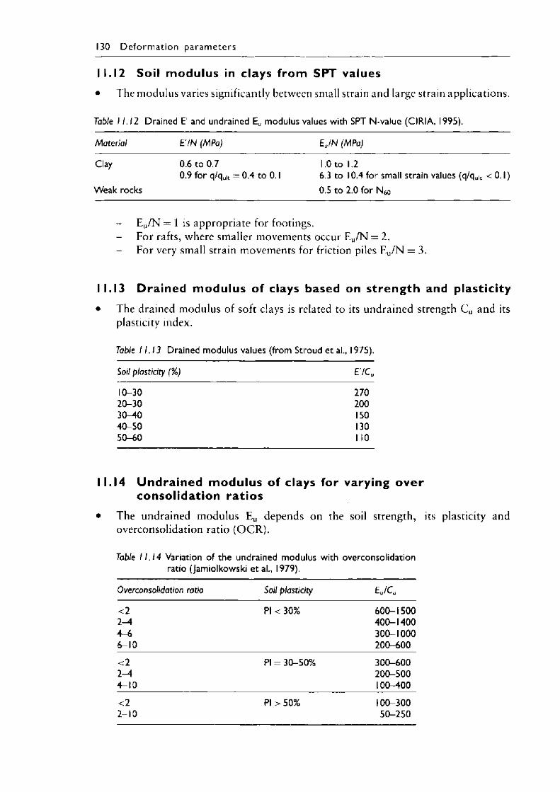
130 D e fo rm a t io n p a ram e te rs
11.12 Soil modulus in clays from SPT values• The modulus varies significantly between small strain and large strain applications.
Table 11.12 Drained E' and undrained E„ modulus values with SPT N-value (CIRIA, 1995).
Material E'/N (MPa) E J N (MPa)
Clay 0.6 to 0.7 1.0 to 1.20.9 for q/qu|t = 0.4 to 0.1 6.3 to 10.4 for small strain values (q/quit < 0.1)
Weak rocks 0.5 to 2.0 for N 6o
Eu/N = 1 is appropriate for footings.- For rafts, where smaller movements occur Eu/N = 2.- For very small strain movements for friction piles Eu/N = 3.
11.13 Drained modulus of clays based on strength and plasticity• The drained modulus of soft clays is related to its undrained strength C u and its
plasticity index.
Table 11.13 Drained modulus values (from Stroud et al., 1975).
Soil plasticity (%) E'/Cu
10-30 27020-30 20030—40 15040-50 13050-60 1 10
11.14 Undrained modulus of clays for varying over consolidation ratios
• The undrained modulus E u depends on the soil strength, its plasticity and overconsolidation ratio (OCR) .
Table 11.14 Variation of the undrained modulus with overconsolidation ratio (jamiolkowski et al., 1979).
Overconsolidation ratio Soil plasticity E J C U
<2 PI < 30% 600-15002—4 400-14004-6 300-10006-10 200-600
<2 PI = 30-50% 300-6002—4 200-5004-10 100-400
<2 PI > 50% 100-3002-10 50-250
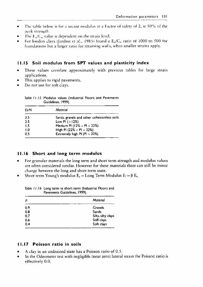
D e fo rm a t io n p a ra m e te rs 131
• The table below is for a secant modulus at a Factor of safety of 2, ie 5 0 % of the peak strength.
• The Eu/Q, value is dependent on the strain level.• For london clays (Jardine et al., 1985) found a Eu/Cu ratio of 1000 to 5 0 0 for
foundations but a larger ratio for retaining walls, when smaller strains apply.
11.15 Soil modulus from SPT values and plasticity index• These values correlate approximately with previous tables for large strain
applications.• This applies to rigid pavements.• Do not use for soft clays.
Table 11.15 Modulus values (Industrial Floors and Pavements Guidelines, 1999).
Es/N Material
3.5 Sands, gravels and other cohesionless soils2.5 Low PI (< 12%)1.5 Medium PI (12% < PI < 22%)1.0 High PI (22% < PI < 32%)0.5 Extremely high PI (PI > 32%)
11.16 Short and long te rm modulus• For granular materials the long term and short term strength and modulus values
are often considered similar. However for these materials there can still be minor change between the long and short term state.
• Short term Young’s modulus Es = Long Term Modulus E| = P Es
Table 11.16 Long term vs short term (Industrial Floors and Pavements Guidelines, 1999).
P Material
0.9 Gravels0.8 Sands0.7 Silts, silty clays0.6 Stiff clays0.4 Soft clays
11.17 Poisson ratio in soils• A clay in an undrained state has a Poisson ratio of 0.5.• In the Odeometer test with negligible (near zero) lateral strain the Poisson ratio is
effectively 0.0.
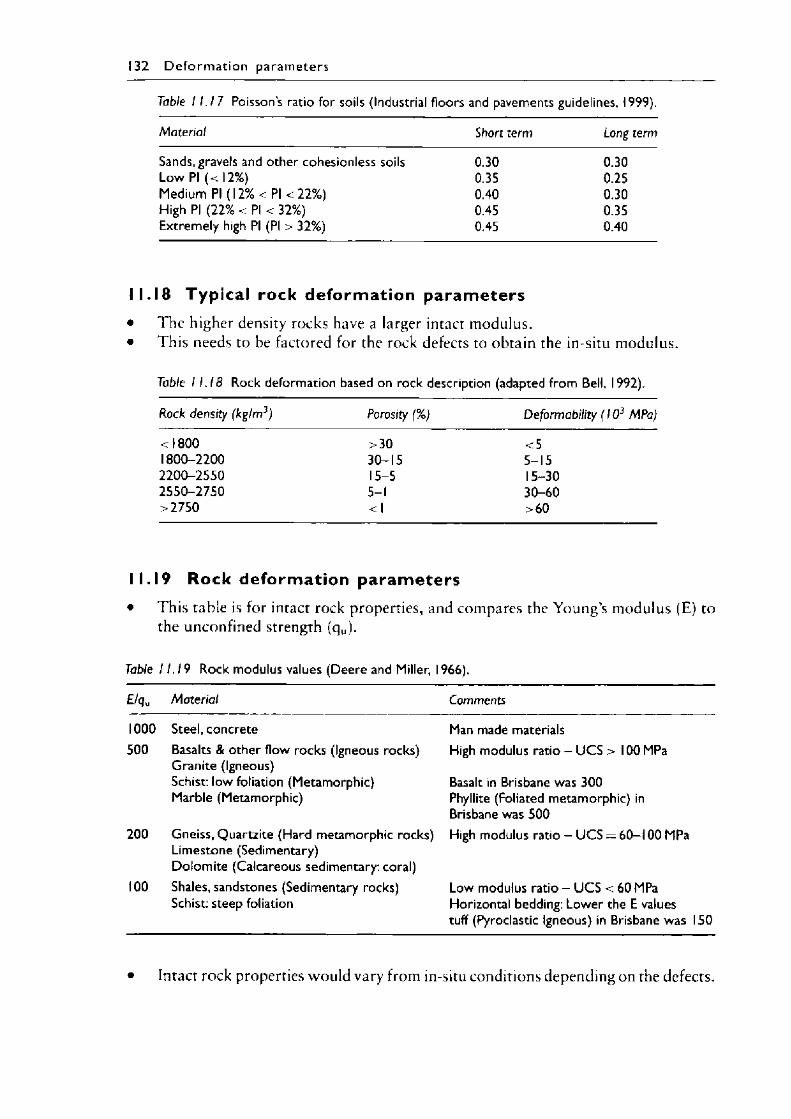
132 D e fo rm a t io n p a ra m e te rs
Table 11.17 Poisson’s ratio for soils (Industrial floors and pavements guidelines, 1999).
Material Short term Long term
Sands, gravels and other cohesionless soils 0.30 0.30Low PI (< 12%) 0.35 0.25Medium PI (12% < PI < 22%) 0.40 0.30High PI (22% < PI < 32%) 0.45 0.35Extremely high PI (PI > 32%) 0.45 0.40
11.18 Typica l rock deformation param eters• The higher density rocks have a larger intact modulus.• This needs to be factored for the rock defects to obtain the in-situ modulus.
Table 11.18 Rock deformation based on rock description (adapted from Bell, 1992).
Rock density (kg/m3) Porosity (%) Deformability (103 MPa)
<1800 >30 <51800-2200 30-15 5-152200-2550 15-5 15-302550-2750 5-1 30-60>2750 <1 >60
11.19 Rock deformation param eters• This table is for intact rock properties, and compares the Young’s modulus (E) to
the unconfined strength (qu).
Table 11.19 Rock modulus values (Deere and Miller, 1966).
E/qu Material Comments
1000 Steel, concrete Man made materials500 Basalts & other flow rocks (Igneous rocks)
Granite (Igneous)High modulus ratio - U C S > 100 MPa
Schist: low foliation (Metamorphic) Basalt in Brisbane was 300Marble (Metamorphic) Phyllite (Foliated metamorphic) in
Brisbane was 500200 Gneiss, Quartzite (Hard metamorphic rocks)
Limestone (Sedimentary)Dolomite (Calcareous sedimentary: coral)
High modulus ratio - U C S — 60-100 MPa
100 Shales, sandstones (Sedimentary rocks) Low modulus ratio - U CS < 60 MPaSchist: steep foliation Horizontal bedding: Lower the E values
tuff (Pyroclastic Igneous) in Brisbane was 150
• Intact rock properties would vary from in-situ conditions depending on the defects.
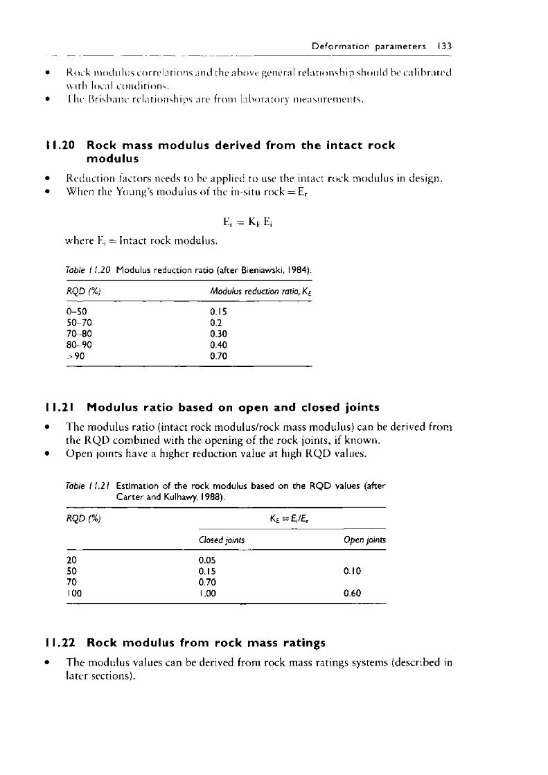
D e fo rm a t io n p a ra m e te rs 133
Rock modulus correlations and the above general relationship should be calibrated with local conditions.I he Brisbane relationships are from laboratory measurements.
11.20 Rock mass modulus derived from the intact rock modulus
• Reduction factors needs to be applied to use the intact rock modulus in design.• When the Young’s modulus of the in-situ rock = Er
Er = Kf Ej
where E, = Intact rock modulus.
Table 11.20 Modulus reduction ratio (after Bieniawski, 1984).
RQD (%) Modulus reduction ratio, Kg
0-50 0.1550-70 0.270-80 0.3080-90 0.40>90 0.70
11.21 Modulus ratio based on open and closed joints• The modulus ratio (intact rock modulus/rock mass modulus) can be derived from
the R Q D combined with the opening of the rock joints, if known.• Open joints have a higher reduction value at high R Q D values.
Table 1 1.21 Estimation of the rock modulus based on the R Q D values (after Carter and Kulhawy, 1988).
RQD (%) K e = E ,IE r
Closed joints Open joints
20 0.0550 0.15 0.1070 0.70100 1.00 0.60
I 1.22 Rock modulus from rock mass ratings• The modulus values can be derived from rock mass ratings systems (described in
later sections).
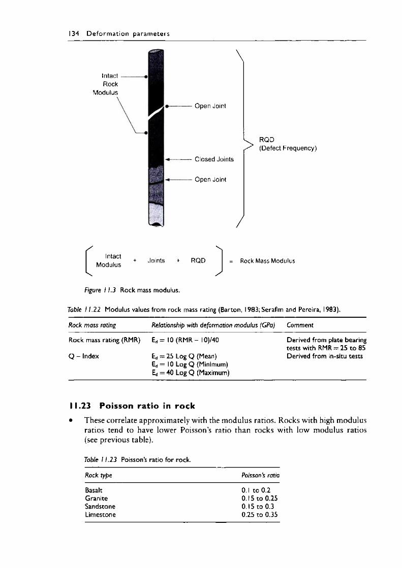
134 D e fo rm a t io n p a ram ete rs
IntactRock
ModulusOpen Joint
>---- Closed Joints
Open Joint
RQD(Defect Frequency)
IntactModulus Joints + RQD Rock Mass Modulus
Figure 1 1.3 Rock mass modulus.
Table 11.22 Modulus values from rock mass rating (Barton, 1983; Serafim and Pereira, 1983).
Rock mass rating Relationship with deformation modulus (GPa) Comment
Rock mass rating (RMR) Ed= 10 (RMR - l0)/40 Derived from plate bearing tests with RMR = 25 to 85
Q - Index Ed = 25 Log Q (Mean)Ed = 10 Log Q (Minimum) Ed = 4 0 Log Q (Maximum)
Derived from in-situ tests
11.23 Poisson ratio in rock• These correlate approximately with the modulus ratios. Rocks with high modulus
ratios tend to have lower Poisson’s ratio than rocks with low modulus ratios (see previous table).
Table 1 1.23 Poisson’s ratio for rock.
Rock type Poisson’s ratio
Basalt 0.1 to 0.2Granite 0.15 to 0.25Sandstone 0.15 to 0.3Limestone 0.25 to 0.35
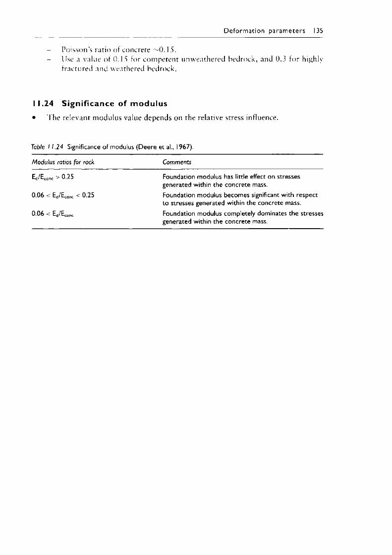
D e fo rm a t io n p a ra m e te rs 135
- Poisson’s ratio of concrete M). 15.- Use a value of 0 .15 for competent unweathered bedrock, and 0.3 for highly
fractured and weathered bedrock.
11.24 Significance of modulus• The relevant modulus value depends on the relative stress influence.
Table 11.24 Significance of modulus (Deere et al., 1967).
Modulus ratios for rock Comments
Ed/Econc > 0.25 Foundation modulus has little effect on stresses generated within the concrete mass.
0.06 < Ed/Econc < 0.25 Foundation modulus becomes significant with respect to stresses generated within the concrete mass.
0.06 < Ed/Econc Foundation modulus completely dominates the stresses generated within the concrete mass.

Earthworks
12.1 Ea rth w o rks issues• The designs construction issues are covered in the table below.• Issues related to pavements are discussed in the next chapter.• Related issues on silopes and retaining walls are covered in later chapters.
Table 12. / Earthworks issues.
Earthwork Issues Comments
Excavatability Covered in this chapter. The material parameter is only 1 indicator ofexcavatability. Type of excavation and plant data also required.
Compaction characteristics Covered in this chapter. Depends on material, type ofexcavation/operating space and plant.
Bulk up Covered in this chapter. Depends on material.Pavements Refer chapter 1 3Slopes Refer chapter 14Retaining walls Refer chapter 20Drainage and erosion Refer chapter 15Geosynthetics Refer chapter 16
12.2 Excavatabil ity• The excavatability depends on the method used as well as the material properties.• Some of these are not mutually exclusive, ie strength may be affected by degree of
weathering, and run direction is relevant mainly for large open excavations, and when dip direction is an issue.
• Geological definition of rock is different form the contractual definition, where production rates are important.
12.3 Excavat ion requ irem ents• The strength of the material is one of the key indicators in assessing the excavation
requirements.• The table provides a preliminary assessment of the likely excavation requirements.
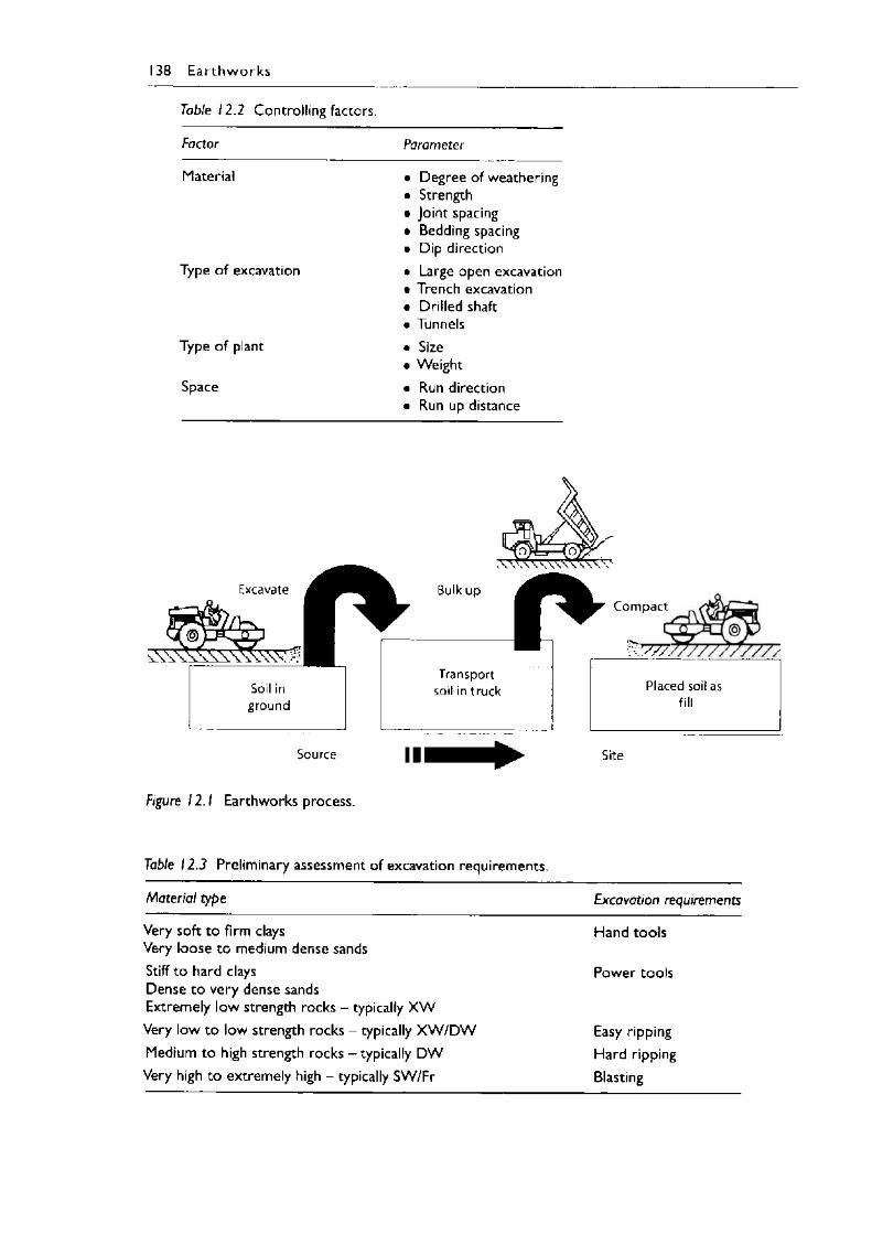
138 E a r th w o r k s
Table 12.2 Controlling factors.
Factor Parameter
Material • Degree of weathering• Strength• Joint spacing• Bedding spacing• Dip direction
Type of excavation • Large open excavation• Trench excavation• Drilled shaft• Tunnels
Type of plant
Space
• Size• Weight• Run direction• Run up distance
Aoyjy
Bulk up
f * Compact
Transport soil in truck
::C777
Placed soil as fill
Source 1 1 Site
Figure 12 .1 Earthworks process.
Table 12.3 Preliminary assessment of excavation requirements.
Material type Excavation requirements
Very soft to firm claysVery loose to medium dense sands
Hand tools
Stiff to hard claysDense to very dense sandsExtremely low strength rocks - typically X W
Power tools
Very low to low strength rocks - typically X W /D W Easy rippingMedium to high strength rocks - typically DW Hard rippingVery high to extremely high - typically SW/Fr Blasting
• The blasting term as used here refers to the difficulty level and can include rock breakers, or expanding grouts.
12.4 Excavat ion character ist ics• The excavatability characteristics based on rock hardness and strength.• The above is combined with its bulk properties (seismic velocity) and joint spacing.
E a r t h w o r k s 139
Table 12.4 Excavation characteristics (Bell, 1992).
Rock hardness description
Unconfined compressive strength (MPa)
Seismic wave velocity (m/s)
Spacing o f joints (mm)
Excavationcharacteristics
Very soft 1.7-3.0 450-1200 <50 Easy rippingSoft 3.0-10 1200-1500 50-300 Hard rippingHard 10-20 1500-1850 300-1000 Very hard rippingVery hard 20-70 1850-2150 1000-3000 Extremely hard
Ripping or blastingExtremely hard >70 >2150 >3000 Blasting
• Table below combines both factors of strength and fractures into one assessment.
12.5 Excavatab i l i ty assessm ent• The excavatability data shown are extracted from charts. It is therefore approxi
mate values only.• Higher strengths combined with closer discontinuity spacing shifts the excavata
bility rating.
Table 12.5 Excavatability assessment (Franklin et al. 1971 with updates from Walton and Wong, 1993).
Parameter Easy digging Marginal digging without blasting
Blast to loosen Blast to fracture
Strength, ls (50) (MPa) <0.1 <0.3 >0.3 >0.3Discontinuity spacing (m) <0.02 <0.2 0.2 to 0.6 >0.6R Q D (%) <10% <90% >90% >90%
• Blast to loosen can be equated to using a rock breaker.• Ripping involves using a tine attached to the rear of the bulldozer.
12.6 Diggabil ity index• The rock weathering term is another term incorporated in this table as well as the
type of equipment (backhoe or excavator).• This table classifies the diggability only. The following table provides the
implication for the type of equipment.
140 E a r th w o rk s
Table 12.6 Diggability index rating (adapted from, Scoble and Muftuoglu, 1984).
Parameter Symbol RankingWeathering W
RatingComplete
0High
5Moderately
15Slight
20Fresh
25
Strength (MPa): UCS Is (50)
S
Rating
<20<0.5
0
20-50 0.5-1.5
5
40-60 1.5-2.0
15
60-1002-3.5
20
>100>3.5
25
Joint spacing (m) jRating
<0.35
0.3-0.615
0.6-1.530
1.5-245
>250
Bedding spacing (m) BRating
<0.10
0.1-0.35
0.3-0.610
0.6-1.520
>1.530
12.7 Diggability classification• The Diggability in terms of the type of plant required uses the Index obtained
from the previous table.
Table 12.7 Diggability classification for excavators (adapted from, Scoble and Muftuoglu, 1984).
Class Ease o f digging
Index(W + S + J + B)
Typical plant which may be used without blasting
Type Example
1 Very Easy <40 Hydraulic backhoe <3 m3 C A T 235DII Easy 40-50 Hydraulic shovel or backhoe <3 m3 C A T 235FS, 235 MEIII Moderately 50-60 Hydraulic shovel or backhoe >3 m3 C A T 245FS, 245 MEIV Difficult 60-70 Hydraulic shovel or backhoe >3 m3:
Short boom of a backhoeC A T 245, O&K RH 40
V Very difficult 70-95 Hydraulic shovel or backhoe >4 m3 Hitachi EX 100VI Extremely
difficult95-100 Hydraulic shovel or backhoe >7 m3 Hitachi EX 1800,
O&K RH 75
12.8 Excavat ions in rock• The assessment of open excavations is different from excavations in limited space,
such as trenches or drilled shafts.• Seismic Wave Velocity - SWV• Unconfined Compressive Strength - UCS• For drilled shafts:
- Limit of earth auger is 15cm penetration in a 5 - minute period —> Replace with Rock Auger.
- Rock Auger to Down-the-hole hammers (Break).
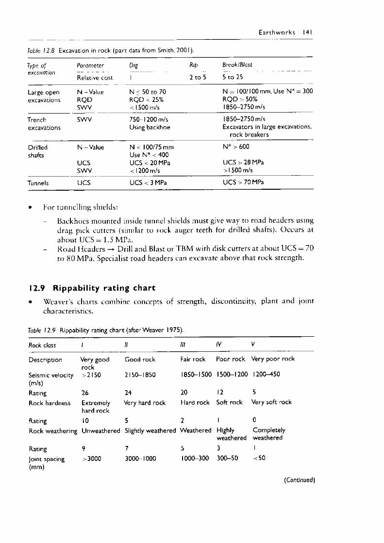
E a r th w o r k s 141
Table 12.8 Excavation in rock (part data from Smith, 2001).
Type o f Parameter Dig Rip Break/Blastexcavation
Relative cost 1 2 to 5 5 to 25
Large open excavations
N -ValueR Q DSW V
N < 50 to 70 RQ D < 25% < 1500 m/s
N = 100/100 mm, Use N* = 300 R Q D > 50%1850-2750 m/s
Trenchexcavations
SW V 750-1200 m/s Using backhoe
1850-2750 m/sExcavators in large excavations,
rock breakers
Drilledshafts
N -Value
U CSSW V
N < 100/75 mm Use N* < 400 UCS < 20 MPa < 1200 m/s
N* > 600
U C S > 28 MPa > 1500 m/s
Tunnels U CS U CS < 3 MPa U CS > 70 MPa
• For tunnelling shields:
- Backhoes mounted inside tunnel shields must give way to road headers usingdrag pick cutters (similar to rock auger teeth for drilled shafts). Occurs at about U C S = 1.5 MPa.Road Headers -> Drill and Blast or T B M with disk cutters at about UCS = 70 to 80 MPa. Specialist road headers can excavate above that rock strength.
12.9 Rippability rating chartWeaver's charts combine concepts of strength, discontinuity, plant and jointcharacteristics
Table 12.9 Rippability rating chart (after Weaver 1975).
Rock class I II III IV
Description Very good Good rock Fair rock Poor rock Very poor rockrock
Seismic velocity >2150 2150—1850 1850—1500 1500—1200 1200—450(m/s)Rating 26 24 20 12 5Rock hardness Extremely Very hard rock Hard rock Soft rock Very soft rock
hard rockRating 10 5 2 I 0Rock weathering Unweathered Slightly weathered Weathered Highly Completely
weathered weatheredRating 9 7 5 3 1Joint spacing >3000 3000-1000 1000—300 300—50 <50(mm)
(Continued)
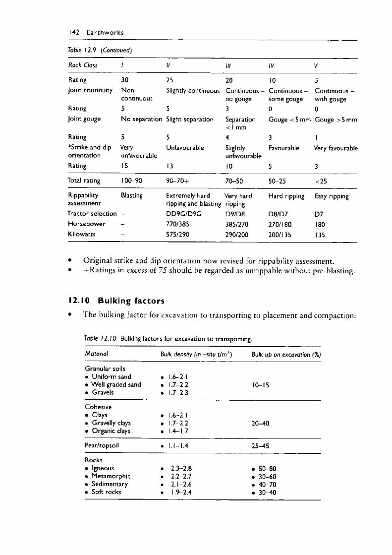
142 E a r th w o rk s
Table 12.9 (Continued)
Rock Class / II III IV V
Rating 30 25 20 10 5Joint continuity Non- Slightly continuous Continuous - Continuous - Continuous -
continuous no gouge some gouge with gougeRating 5 5 3 0 0Joint gouge No separation Slight separation Separation Gouge <5 mm Gouge >5 mm
< 1 mmRating 5 5 4 3 1*Strike and dip Very Unfavourable Slightly Favourable Very favourableorientation unfavourable unfavourableRating 15 13 10 5 3
Total rating 100-90 90-70+ 70-50 50-25 <25
Rippability Blasting Extremely hard Very hard Hard ripping Easy rippingassessment ripping and blasting rippingTractor selection - DD 9G/D9G D9/D8 D8/D7 D7Horsepower - 770/385 385/270 270/180 180Kilowatts - 575/290 290/200 200/135 135
• Original strike and dip orientation now revised for rippability assessment.• +Ratings in excess of 75 should be regarded as unrippable without pre-blasting.
12.10 Bulking factors• The bulking factor for excavation to transporting to placement and compaction:
Table 12.10 Bulking factors for excavation to transporting.
Material Bulk density (in -situ t/m ') Bulk up on excavation (%)
Granular soils• Uniform sand • 1.6-2.1• Well graded sand • 1.7-2.2 10-15• Gravels • 1.7-2.3
Cohesive• Clays • 1.6-2.1• Gravelly clays • 1.7-2.2 20-40• Organic clays • 1.4-1.7
Peat/topsoil • 1.1-1.4 25—45
Rocks• Igneous • 2.3-2.8 • 50-80• Metamorphic • 2.2-2.7 • 30-60• Sedimentary • 2.1-2.6 • 40-70• Soft rocks • 1.9-2.4 • 30—40
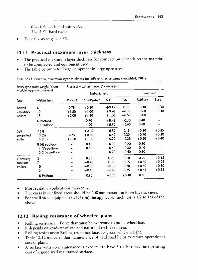
E a r th w o r k s 143
0 % — 10% soils and soft rocks.5 % - 2 0 % hard rocks.
• Typically wastage is ~ 5 % .
12.11 Practica l m ax im um layer thickness• The practical maximum layer thickness for compaction depends on the material
to be compacted and equipment used.• The table below is for large equipment in large open areas.
Table 12.11 Practical maximum layer thickness for different roller types (Forssblad, 1981).
Roller type static weight (drum Practical maximum layer thickness (m) module weight in brackets)
Embankment Pavement.
Type Weight (ton) Rock fill Sand/gravel Silt Clay Subbase Base
Towed 6 0.75 +0.60 +0.45 0.25 -0 .40 +0.30vibratory 10 + 1.50 + 1.00 +0.70 -0 .35 -0 .60 +0.40rollers 15 +2.00 + 1.50 + 1.00 -0 .50 -0 .80 —
6 Padfoot - 0.60 +0.45 +0.30 0.40 -10 Padfoot - 1.00 +0.70 +0.40 0.60 —
Self 7(3) _ +0.40 +0.30 0.15 +0.30 +0.25propelled 10(5) 0.75 +0.50 +0.40 0.20 +0.40 +0.30roller 15(10) + 1.50 + 1.00 +0.70 +0.35 +0.60 +0.40
8 (4) padfoot - 0.40 +0.30 +0.20 0.30 -1 1 (7) padfoot - 0.60 +0.40 +0.30 0.40 —15 (10) padfoot - 1.00 +0.70 +0.40 0.60 —
Vibratory 2 — 0.30 0.20 0.10 0.20 +0.15tandem 7 - +0.40 0.30 0.15 +0.30 +0.25rollers 10 — +0.50 +0.35 0.20 +0.40 +0.30
13 - +0.60 +0.45 0.25 +0.45 +0.3518 Padfoot - 0.90 +0.70 +0.40 0.60 -
• Most suitable applications marked + .• Thickness in confined areas should be 2 0 0 mm maximum loose lift thickness.• For small sized equipment ( < 1 .5 ton) the applicable thickness is 1/2 to 1/3 of the
above.
12.12 Rolling resistance of wheeled plant• Rolling resistance = Force that must be overcome to pull a wheel load.• It depends on gradient of site and nature of trafficked area.• Rolling resistance = Rolling resistance factor x gross vehicle weight.• Table 12 .12 indicates that maintenance of haul road helps to reduce operational
cost of plant.• A surface with no maintenance is expected to have 5 to 10 times the operating
cost of a good well maintained surface.
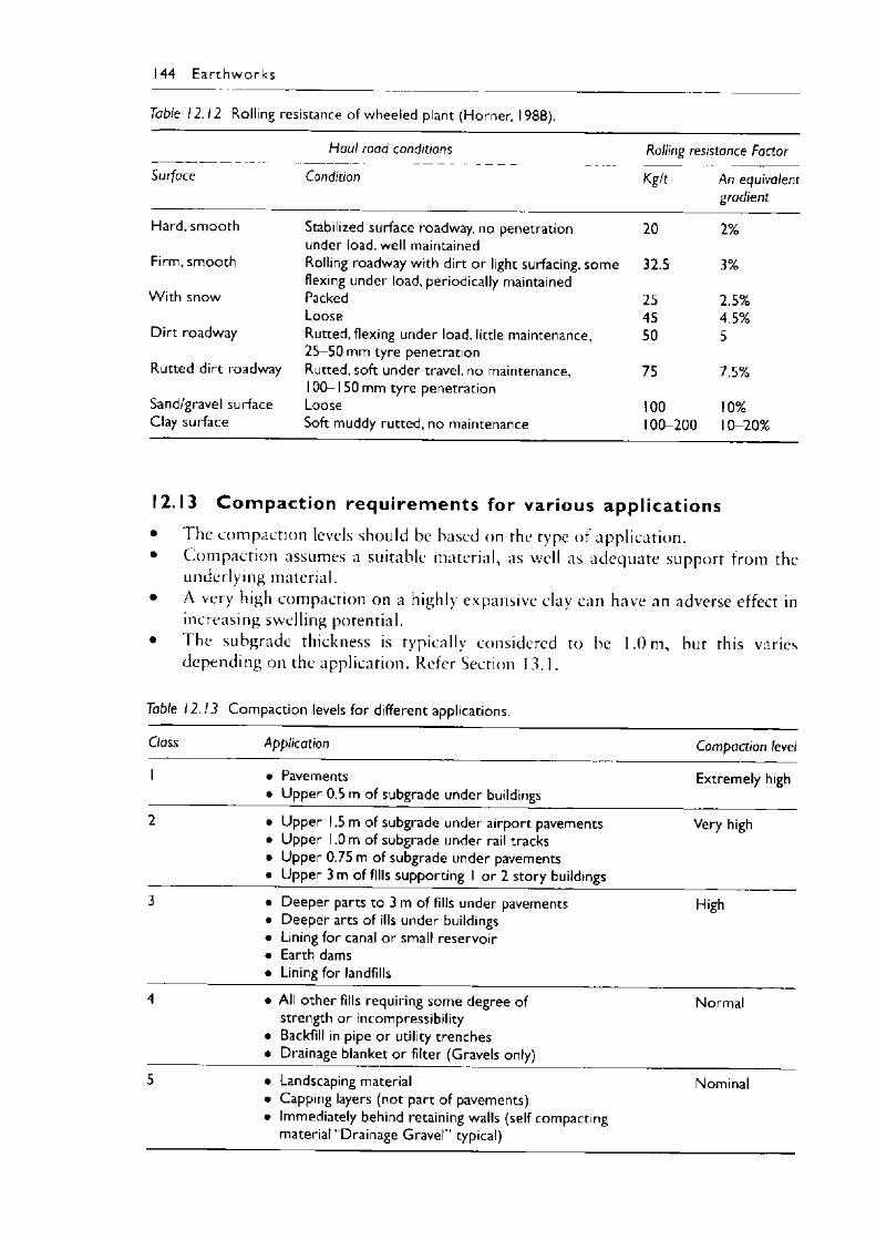
144 E a r th w o r k s
Table 12.12 Rolling resistance of wheeled plant (Horner, 1988).
Haul road conditions Rolling resistance Factor
Surface Condition Kg/t An equivalent gradient
Hard, smooth Stabilized surface roadway, no penetration under load, well maintained
Firm, smooth Rolling roadway with dirt or light surfacing, some flexing under load, periodically maintained
With snow Packed Loose
Dirt roadway Rutted, flexing under load, little maintenance, 25-50 mm tyre penetration
Rutted dirt roadway Rutted, soft under travel, no maintenance,100-150 mm tyre penetration
Sand/gravel surface LooseClay surface Soft muddy rutted, no maintenance
20 2%
32.5 3%
25 2.5%45 4.5%50 5
75 7.5%
100 10% 100-200 10-20%
12.13 Com pact ion requ irem ents for various applications• 1 he compaction levels should be based on the type of application.• Compaction assumes a suitable material, as well as adequate support from the
underlying material.• A very high compaction on a highly expansive clay can have an adverse effect in
increasing swelling potential.• I he subgrade thickness is typically considered to be 1.0 m, but this varies
depending on the application. Refer Section 13.1.
Table 12.13 Compaction levels for different applications.
Class Application Compaction level
1 • Pavements• Upper 0.5 m of subgrade under buildings
Extremely high
2 • Upper 1.5 m of subgrade under airport pavements• Upper 1.0 m of subgrade under rail tracks• Upper 0.75 m of subgrade under pavements• Upper 3 m of fills supporting 1 or 2 story buildings
Very high
3 • Deeper parts to 3 m of fills under pavements• Deeper arts of ills under buildings• Lining for canal or small reservoir• Earth dams• Lining for landfills
High
4 • All other fills requiring some degree of strength or incompressibility
• Backfill in pipe or utility trenches• Drainage blanket or filter (Gravels only)
Normal
5 • Landscaping material• Capping layers (not part of pavements)• Immediately behind retaining walls (self compacting
material “Drainage Gravel" typical)
Nominal
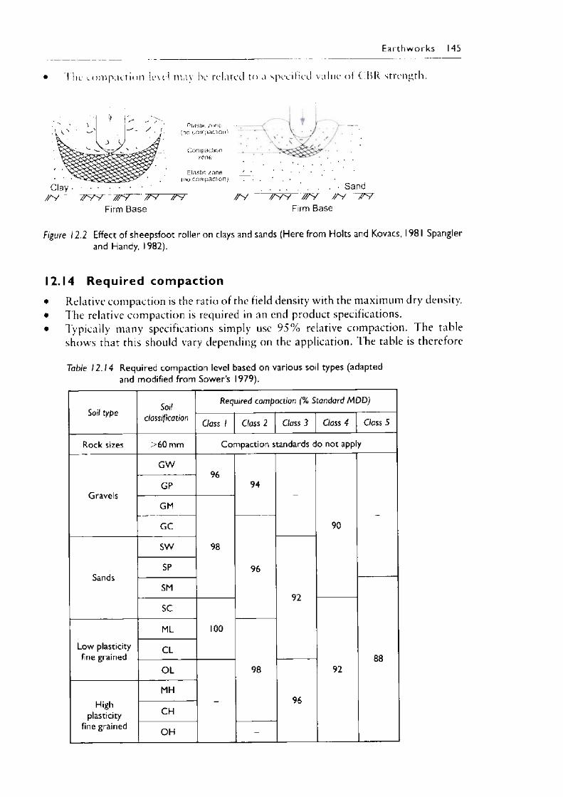
E a r th w o r k s 145
• The compaction level may he related to a specified value of C.BR strength.
Plastic /one (no compaction)
Compaction/one
Elastic zone (no compaction)
2*7 TFW"' JF? 7F7~Firm B ase
~7FT. . • • Sand
/ V ’ / / W //FV /F/ TV Firm Base
Figure 12.2 Effect of sheepsfoot roller on clays and sands (Here from Holts and Kovacs, 19 8 1 Spangler and Handy, 1982).
12.14 Required compaction• Relative compaction is the ratio of the field density with the maximum dry density.• The relative compaction is required in an end product specifications.• Typically many specifications simply use 9 5 % relative compaction. The table
shows that this should vary depending on the application. The table is therefore
Table 12.14 Required compaction level based on various soil types (adapted and modified from Sower’s 1979).
Soil type SoilRequired compaction (% Standard MDD)
classification Class 1 Class 2 Class 3 Class 4 Class 5
Rock sizes >60 mm Compaction standards do not appiy
GW96
GravelsGP 94
GM
GC 90
SW 98
SandsSP 96
SM92
SC
ML 100
Low plasticity fine grained CL
88OL 98 92
MH96High
plasticity CHfine grained OH -
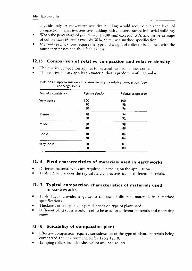
146 E a r th w o rk s
a guide only. A movement sensitive building would require a higher level of compaction, than a less sensitive building such as a steel framed industrial building.
• When the percentage of gravel sizes (> 2 0 0 mm) exceeds 1 5 % , and the percentage of cobble sizes (60 mm) exceeds 3 0 % , then use a method specification.
• Method specifications require the type and weight of roller to be defined with thenumber of passes and the lift thickness.
12.15 Com par ison of relat ive compaction and relative density• The relative compaction applies to material with some fines content.• The relative density applies to material that is predominantly granular.
Table 12.15 Approximation of relative density to relative compaction (Lee and Singh, 19 7 1).
Granular consistency Relative density Relative compaction
Very dense 100 10090 9880 96
Dense 70 9460 92
Medium 50 9840 88
Loose 30 8620 84
Very loose 10 820 80
12.16 Field character ist ics of materia ls used in earthworks• Different material types are required depending on the application.• Table 12.16 provides the typical field characteristics for different materials.
12.17 Typical compaction character ist ics of mater ia ls used in earthworks
• Table 12.17 provides a guide to the use of different materials in a method specifications.
• Thickness of compacted layers depends on type of plant used.• Different plant types would need to be used for different materials and operating
room.
12.18 Suitabil ity of com pact ion plant• Effective compaction requires consideration of the type of plant, materials being
compacted and environment. Refer Table 12.18.• Tamping rollers includes sheepsfoot and pad rollers.
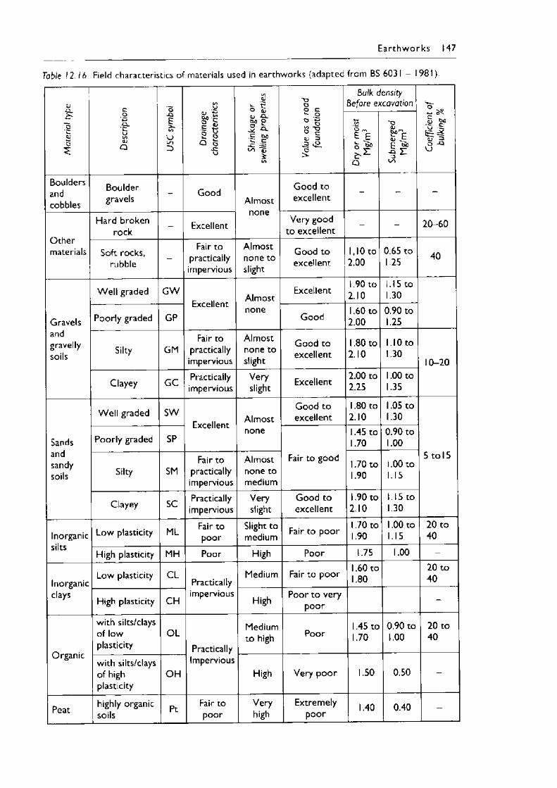
E a r th w o rk s 147
Table 12.16 Field characteristics of materials used in earthworks (adapted from BS 6031 - 1981).M
ater
ial
type
Desc
riptio
n
USC
sym
bol
Drai
nage
char
acte
ristic
s
Shrin
kage
or
sw
elling
pr
oper
ties
oo cBulk density
Before excavation
Coef
ficien
t of
bu
lking
%*“* °
° o 8 -g <u =3 -2
<y)
I ' e
Q
<uSTc<UP w> -Q Z3uo
Bouldersandcobbles
Bouldergravels - Good
Almostnone
Good to excellent - - -
Othermaterials
Hard broken rock - Excellent Very good
to excellent - - 20-60
Soft rocks, rubble -
Fair to practically impervious
Almost none to slight
Good to excellent
1,10 to 2.00
0.65 to 1 25 40
Gravelsandgravellysoils
W ell graded G WExcellent Almost
none
Excellent 1.90 to 2.10
1.15 to 1.30
Poorly graded GP Good 1.60 to 2.00
0.90 to 1.25
Silty GMFair to
practically impervious
Almost none to slight
Good to excellent
1.80 to 2.10
1.10 to 1.30
10-20
Clayey G C Practicallyimpervious
Veryslight Excellent 2.00 to
2.251.00 to 1.35
Sandsandsandysoils
W ell graded SWExcellent Almost
none
Good to excellent
1.80 to 2.10
1.05 to 1.30
5 to 15Poorly graded SP
Fair to good
1.45 to 1.70
0.90 to 1.00
Silty SMFair to
practically impervious
Almost none to medium
1.70 to 1.90
1.00 to 1.15
Clayey SC Practicallyimpervious
Veryslight
Good to excellent
1.90 to 2.10
1.15 to 1.30
Inorganicsilts
Low plasticity ML Fair to poor
Slight to medium Fair to poor 1.70 to
1.901.00 to 1.15
20 to 40
High plasticity MH Poor High Poor 1.75 1.00 -
Inorganicclays
Low plasticity C LPractically
impervious
Medium Fair to poor 1.60 to 1.80
20 to 40
High plasticity CH High Poor to very poor -
Organic
with silts/clays of low plasticity
O LPractically
Medium to high Poor
1.45 to 1.70
0.90 to 1.00
20 to 40
with silts/clays of high plasticity
O HImpervious
High Very poor 1.50 0.50 -
Peat highly organic soils Pt Fair to
poorVeryhigh
Extremelypoor 1.40 0.40 -
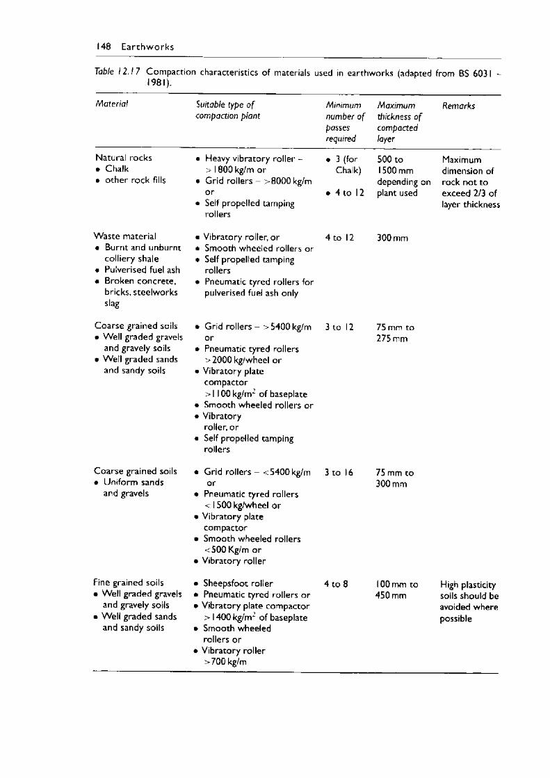
148 E a r t h w o r k s
Table 12.1 7 Compaction characteristics of materials used in earthworks (adapted from BS 603 1 - 1981).
Material Suitable type o f compaction plant
Minimum number o f passes required
Maximum thickness o f compacted layer
Remarks
Natural rocks• Chalk• other rock fills
• Heavy vibratory roller - > 1800 kg/m or
• Grid rollers - >8000 kg/m or
• Self propelled tamping rollers
• 3 (for Chalk)
• 4 to 12
500 to 1500 mm depending on plant used
Maximum dimension of rock not to exceed 2/3 of layer thickness
Waste material• Burnt and unburnt
colliery shale• Pulverised fuel ash• Broken concrete,
bricks, steelworks slag
• Vibratory roller, or• Smooth wheeled rollers or• Self propelled tamping
rollers• Pneumatic tyred rollers for
pulverised fuel ash only
4 to 12 300 mm
Coarse grained soils• Well graded gravels
and gravely soils• Well graded sands
and sandy soils
• Grid rollers - >5400 kg/m or
• Pneumatic tyred rollers >2000 kg/wheel or
• Vibratory plate compactor> 1 100 kg/m2 of baseplate
• Smooth wheeled rollers or• Vibratory
roller, or• Self propelled tamping
rollers
3 to 12 75 mm to 275 mm
Coarse grained soils • Uniform sands
and gravels
• Grid rollers - <5400 kg/m or
• Pneumatic tyred rollers < 1500 kg/wheel or
• Vibratory plate compactor
• Smooth wheeled rollers <500 Kg/m or
• Vibratory roller
3 to 16 75 mm to 300 mm
Fine grained soils• Well graded gravels
and gravely soils• Well graded sands
and sandy soils
• Sheepsfoot roller• Pneumatic tyred rollers or• Vibratory plate compactor
> 1400 kg/m2 of baseplate• Smooth wheeled
rollers or• Vibratory roller
>700 kg/m
4 to 8 100 mm to 450 mm
High plasticity soils should be avoided where possible
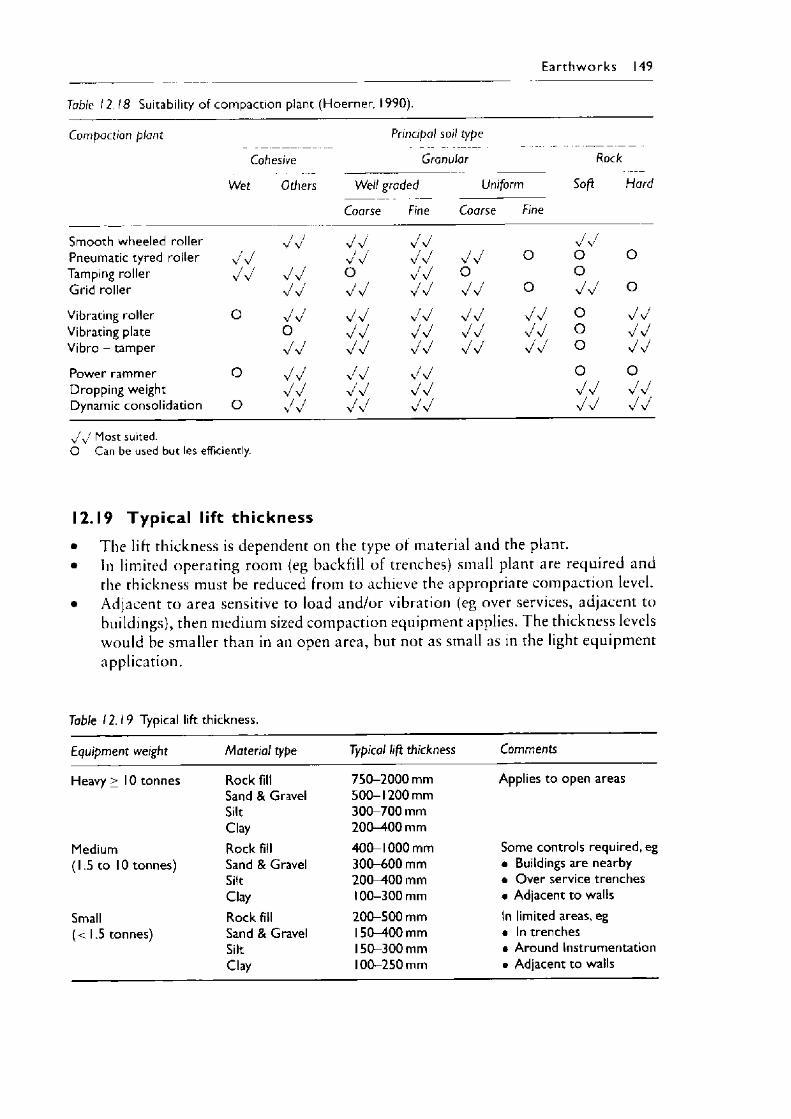
E a r t h w o r k s 149
Table 12.18 Suitability of compaction plant (Hoerner, 1990).
Compaction plant Principal soil type
Cohesive Granular Rock
Wet Others Well graded Uniform Soft Hard
Coarse Fine Coarse Fine
Smooth wheeled roller VV vv VV VVPneumatic tyred roller VV V V VV VV O o OTamping roller VV v v o V V o oGrid roller yy V V V V VV O VV O
Vibrating roller o V V V V vv VV yy o VVVibrating plate o V V V V VV v V o V VVibro - tamper V V V V vv VV y/y/ o VVPower rammer o vv V V V V o oDropping weight v v v v V V VV v/VDynamic consolidation o V V V V V V VV nVJ y / Most suited.O Can be used but les efficiently.
12.19 Typica l lift thickness• The lift thickness is dependent on the type of material and the plant.• In limited operating room (eg backfill of trenches) small plant are required and
the thickness must be reduced from to achieve the appropriate compaction level.• Adjacent to area sensitive to load and/or vibration (eg over services, adjacent to
buildings), then medium sized compaction equipment applies. The thickness levels would be smaller than in an open area, but not as small as in the light equipment application.
Table 12.19 Typical lift thickness.
Equipment weight Material type Typical lift thickness Comments
Heavy > 10 tonnes Rock fill Sand & Gravel Silt Clay
750-2000 mm 500-1200 mm 300-700 mm 200-400 mm
Applies to open areas
Medium Rock fill 400-1000 mm Some controls required, eg(1.5 to 10 tonnes) Sand & Gravel 300-600 mm • Buildings are nearby
Silt 200-400 mm • O ver service trenchesClay 100-300 mm • Adjacent to walls
Small Rock fill 200-500 mm In limited areas, eg(< 1.5 tonnes) Sand & Gravel 150-400 mm • In trenches
Silt 150-300 mm • Around InstrumentationClay 100-250 mm • Adjacent to walls
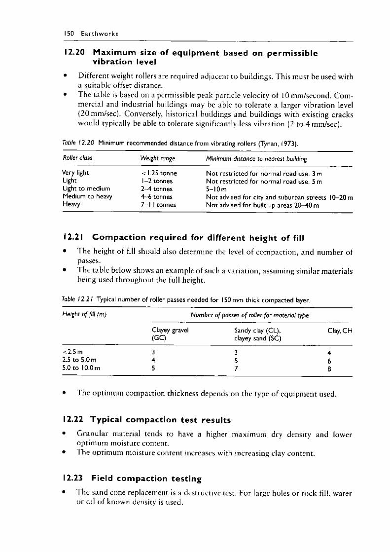
150 E a r th w o r k s
12.20 Maximum size of equipment based on permiss ib le vibration level
• Different weight rollers are required adjacent to buildings. This must be used with a suitable offset distance.
• The table is based on a permissible peak particle velocity of 10 mm/second. C o m mercial and industrial buildings may be able to tolerate a larger vibration level (20 mm/sec). Conversely, historical buildings and buildings with existing cracks would typically be able to tolerate significantly less vibration (2 to 4 mm/sec).
Table 12.20 Minimum recommended distance from vibrating rollers (Tynan, 1973).
Roller class Weight range Minimum distance to nearest building
Very light < 1.25 tonne Not restricted for normal road use. 3 mLight 1-2 tonnes Not restricted for normal road use. 5 mLight to medium 2-4 tonnes 5-10 mMedium to heavy 4-6 tonnes Not advised for city and suburban streets l0 -20mHeavy 7-1 1 tonnes Not advised for built up areas 20—40 m
12.21 C om pact ion required for different height of fill• 1 he height of fill should also determine the level of compaction, and number of
passes.• The table below shows an example of such a variation, assuming similar materials
being used throughout the full height.
Table 12 .2 1 Typical number of roller passes needed for 150 mm thick compacted layer.
Height o f fill (m) Number o f passes o f roller for material type
Clayey gravel (GC)
Sandy clay (CL), clayey sand (SC)
Clay, CH
<2.5 m 3 3 42.5 to 5.0 m 4 5 65.0 to 10.0 m 5 7 8
• The optimum compaction thickness depends on the type o f equipment used.
12.22 Typica l compaction test results• Granular material tends to have a higher maximum dry density and lower
optimum moisture content.• The optimum moisture content increases with increasing clay content.
12.23 Field compaction testing• The sand cone replacement is a destructive test. For large holes or rock fill, water
or oil of known density is used.
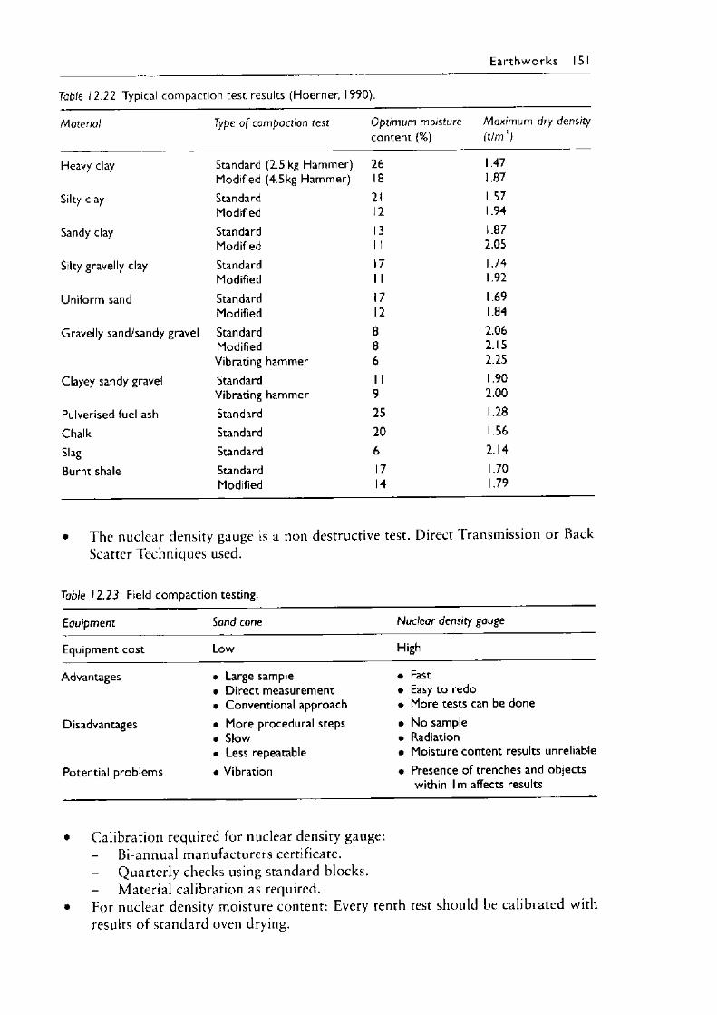
E a r t h w o r k s 151
Table 12.22 Typical compaction test results (Hoerner, 1990).
Material Type o f compaction test Optimum moisture Maximum dry densitycontent (%) (t/m ')
Heavy clay Standard (2.5 kg Hammer) 26 1.47Modified (4.5kg Hammer) 18 1.87
Silty clay Standard 21 1.57Modified 12 1.94
Sandy clay Standard 13 1.87Modified 1 1 2.05
Silty gravelly clay Standard 17 1.74Modified 1 1 1.92
Uniform sand Standard 17 1.69Modified 12 1.84
Gravelly sand/sandy gravel Standard 8 2.06Modified 8 2.15Vibrating hammer 6 2.25
Clayey sandy gravel Standard 1 1 1.90Vibrating hammer 9 2.00
Pulverised fuel ash Standard 25 1.28Chalk Standard 20 1.56Slag Standard 6 2.14Burnt shale Standard 17 1.70
Modified 14 1.79
• The nuclear density gauge is a non destructive test. Direct Transmission or Back Scatter Techniques used.
Table 12.23 Field compaction testing.
Equipment Sand cone Nuclear density gauge
Equipment cost Low High
Advantages
Disadvantages
Potential problems
• Large sample• Direct measurement• Conventional approach• More procedural steps• Slow• Less repeatable• Vibration
• Fast• Easy to redo• More tests can be done• No sample• Radiation• Moisture content results unreliable• Presence of trenches and objects
within 1 m affects results
• Calibration required for nuclear density gauge:- Bi-annual manufacturers certificate.- Quarterly checks using standard blocks.
Material calibration as required.• For nuclear density moisture content: Every tenth test should be calibrated with
results of standard oven drying.
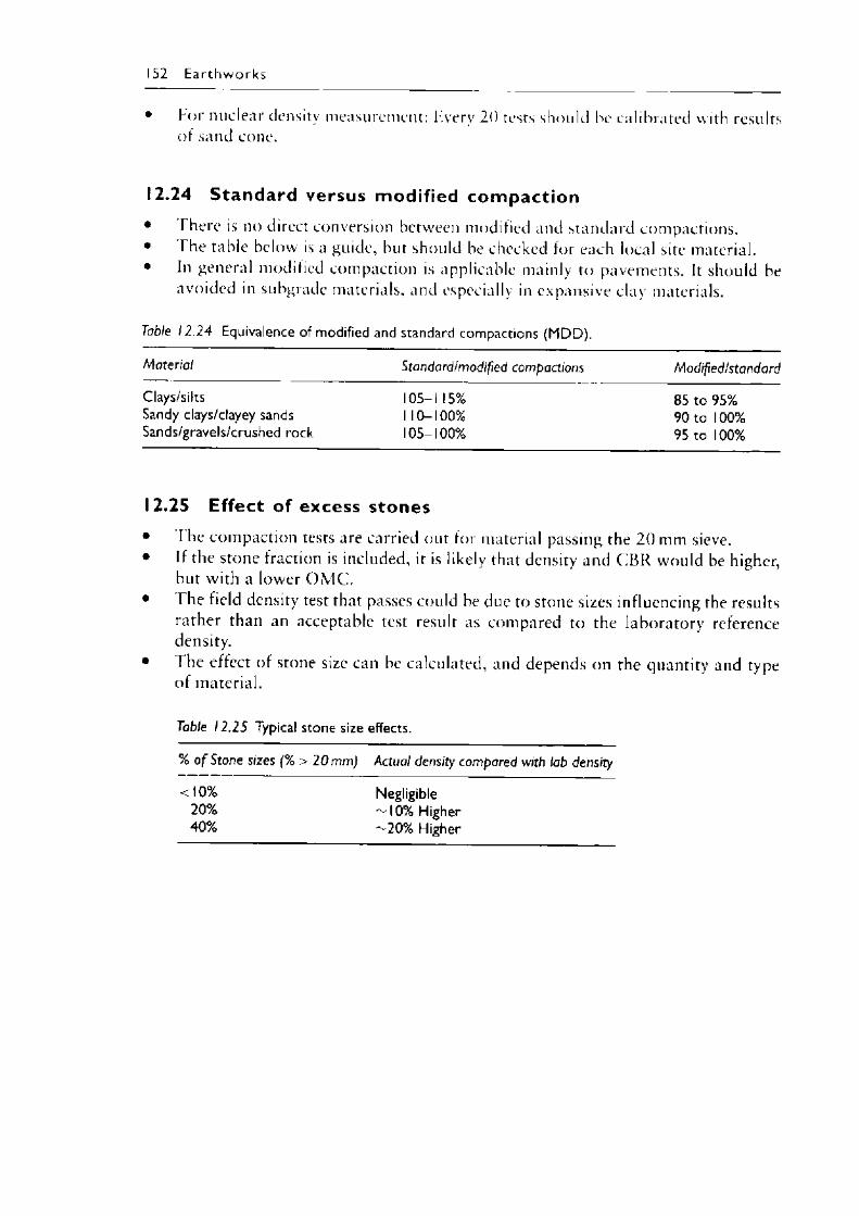
152 E a r t h w o r k s
• For nuclear density measurement: F.verv 20 tests should he calibrated with results of sand cone.
12.24 Standard versus modified compaction• There is no direct conversion between modified and standard compactions.• The table below is a guide, but should be checked for each local site material.• In general modified compaction is applicable mainly to pavements. It should be
avoided in subgrade materials, and especially in expansive clay materials.
Table 12 .24 Equivalence of modified and standard compactions (MDD).
Material Standard/modified compactions Modified/standard
Clays/silts 105-115% 85 to 95%Sandy clays/clayey sands 110-100% 90 to 100%Sands/gravels/crushed rock 105-100% 95 to 100%
12.25 Effect of excess stones• I he compaction tests are carried out for material passing the 2 0 mm sieve.• If the stone fraction is included, it is likely that density and C B R would be higher,
but with a lower O M C .• The field density test that passes could be due to stone sizes influencing the results
rather than an acceptable test result as compared to the laboratory reference density.
• The effect of stone size can be calculated, and depends on the quantity and type of material.
Table 12.25 Typical stone size effects.
% o f Stone sizes (% > 20 mm) Actual density compared with lab density
<10% Negligible20% ~ I0% Higher40% ~20% Higher
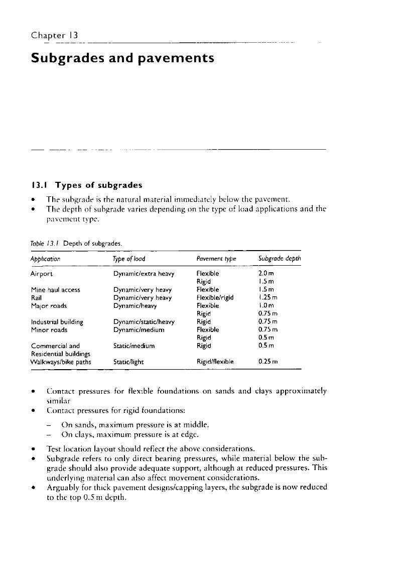
Chapter I 3
Subgrades and pavements
13.1 T yp es of subgrades• The subgrade is the natural material immediately below the pavement.• The depth of subgrade varies depending on the type of load applications and the
pavement type.
Table 13 .1 Depth of subgrades.
Application Type o f load Pavement type Subgrade depth
Airport Dynamic/extra heavy Flexible 2.0 mRigid 1.5 m
Mine haul access Dynamic/very heavy Flexible 1.5 mRail Dynamic/very heavy Flexible/rigid 1.25 mMajor roads Dynamic/heavy Flexible 1.0 m
Rigid 0.75 mIndustrial building Dynamic/static/heavy Rigid 0.75 mMinor roads Dynamic/medium Flexible 0.75 m
Rigid 0.5 mCommercial and Static/medium Rigid 0.5 mResidential buildingsWalkways/bike paths Static/light Rigid/flexible 0.25 m
• Contact pressures for flexible foundations on sands and clays approximately similar
• Contact pressures for rigid foundations:
- On sands, maximum pressure is at middle.On clays, maximum pressure is at edge.
• Test location layout should reflect the above considerations.• Subgrade refers to only direct bearing pressures, while material below the sub
grade should also provide adequate support, although at reduced pressures. This underlying material can also affect movement considerations.
• Arguably for thick pavement designs/capping layers, the subgrade is now reduced to the top 0.5 m depth.
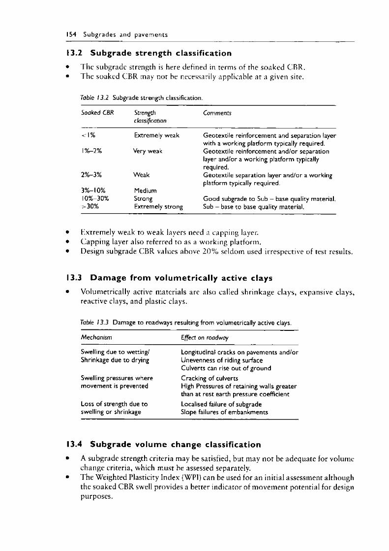
154 Subgrades and pavem ents
13.2 Subgrade strength classification• The suhgrade strength is here defined in terms of the soaked CBR.• The soaked CBR may not be necessarily applicable at a given site.
Table 13.2 Subgrade strength classification.
Soaked CBR Strengthclassification
Comments
<1% Extremely weak Geotextile reinforcement and separation layer with a working platform typically required.
l%-2% Very weak Geotextile reinforcement and/or separation layer and/or a working platform typically required.
2%-3% Weak Geotextile separation layer and/or a working platform typically required.
3 % - 10% Mediuml0%-30% Strong Good subgrade to Sub - base quality material.>30% Extremely strong Sub - base to base quality material.
• Kxtremely weak to weak layers need a capping layer.• Capping layer also referred to as a working platform.• Design subgrade CBR values above 2 0 % seldom used irrespective of test results.
13.3 D am age from volumetr ica l ly active clays• Volumetrically active materials are also called shrinkage clays, expansive clays,
reactive clays, and plastic clays.
Table 13.3 Damage to roadways resulting from volumetrically active clays.
Mechanism Effect on roadway
Swelling due to wetting/ Longitudinal cracks on pavements and/orShrinkage due to drying Unevenness of riding surface
Culverts can rise out of groundSwelling pressures where Cracking of culvertsmovement is prevented High Pressures of retaining walls greater
than at rest earth pressure coefficientLoss of strength due to Localised failure of subgradeswelling or shrinkage Slope failures of embankments
13.4 Subgrade volume change classification• A subgrade strength criteria may be satisfied, but may not be adequate for volume
change criteria, which must be assessed separately.• The Weighted Plasticity Index (WPI) can be used for an initial assessment although
the soaked CBR swell provides a better indicator of movement potential for design purposes.
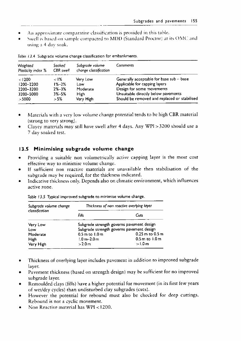
Subgrades and p avem ents 155
• An approximate comparative classification is provided in this table.• Swell is based on sample compacted to M D D (Standard Proctor) at its OMC. and
using a 4 day soak.
Table 13.4 Subgrade volume change classification for embankments.
Weighted Soaked Subgrade volume CommentsPlasticity index % CBR swell change classification
<1200 <1% Very Low Generally acceptable for base sub - base1200-2200 \%-2% Low Applicable for capping layers2200-3200 2%-3% Moderate Design for some movements3200-5000 3%-5% High Unsuitable directly below pavements>5000 >5% Very High Should be removed and replaced or stabilised
• Materials with a very low volume change potential tends to be high CBR material (strong to very strong).
• Clayey materials may still have swell after 4 days. Any WPI > 3 2 0 0 should use a 7 day soaked test.
13.5 Minimising subgrade volume change• Providing a suitable non volumetrically active capping layer is the most cost
effective way to minimise volume change.• If sufficient non reactive materials are unavailable then stabilisation of the
subgrade may be required, for the thickness indicated.• Indicative thickness only. Depends also on climatic environment, which influences
active zone.
Table 13.5 Typical improved subgrade to minimise volume change.
Subgrade volume change Thickness o f non reactive overlying layerclassification ------------------------------------------------------
Fills Cuts
Very Low Subgrade strength governs pavement designLow Subgrade strength governs pavement designModerate 0.5 m to 1.0 m 0.25 m to 0.5 mHigh 1.0 m-2.0 m 0.5 m to 1.0 mVery High >2.0 m > 1.0 m
• Thickness of overlying layer includes pavement in addition to improved subgrade layer.
• Pavement thickness (based on strength design) may be sufficient for no improved subgrade layer.
• Remoulded clays (fills) have a higher potential for movement (in its first few years of wet/dry cycles) than undisturbed clay subgrades (cuts).
• However the potential for rebound must also be checked for deep cuttings. Rebound is not a cyclic movement.
• Non Reactive material has WPI < 1 2 0 0 .
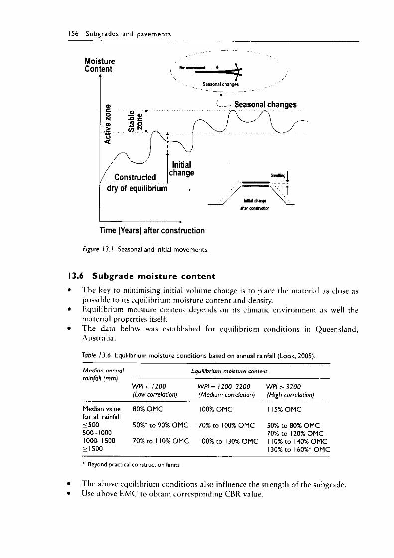
156 Subgrades and pavem ents
Figure 13.1 Seasonal and initial movements.
13.6 Subgrade moisture content• T he key to minimising initial volume change is to place the material as close as
possible to its equilibrium moisture content and density.• Equilibrium moisture content depends on its climatic environment as well the
material properties itself.• The data below was established for equilibrium conditions in Queensland,
Australia.
Table 13.6 Equilibrium moisture conditions based on annual rainfall (Look, 2005).
Median annual rainfall (mm)
Equilibrium moisture content
WP/< 1200 (Low correlation)
W P I= 1200-3200 (Medium correlation)
WPI > 3200 (High correlation)
Median valuefor all rainfall<500500-10001000-1500>1500
80% O M C
50%* to 90% O M C
70% to 1 10% O M C
100% OM C
70% to 100% O M C
100% to 130% O M C
1 15% O M C
50% to 80% OM C 70% to 120% O M C 1 10% to 140% O M C 130% to 160%* O M C
* Beyond practical construction limits
• 1 he above equilibrium conditions also influence the strength of the subgrade.• Use above E M C to obtain corresponding CBR value.
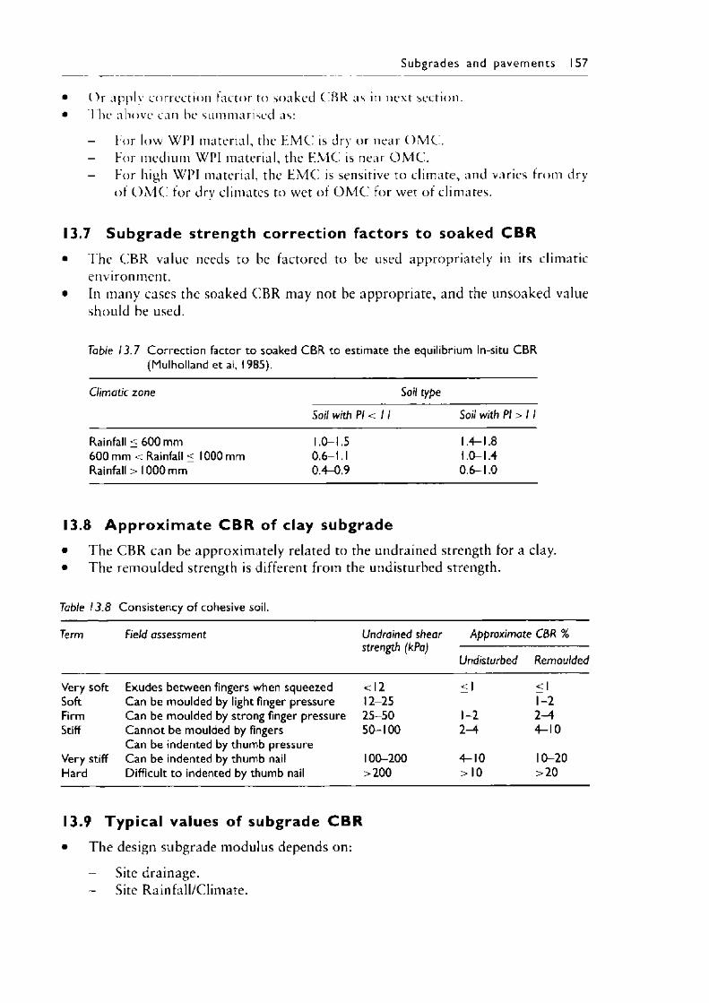
Subgrades and pavem en ts 157
• Or apply correction factor to soaked CBR as in next section.• I lie above can be summarised as:
l o r low WPI material, the E M C is dry or near O M C .For medium WPI material, the E M C is near O M C .For high WPI material, the E M C is sensitive to climate, and varies from dryof O M C for dry climates to wet of OMC' for wet of climates.
13.7 Subgrade strength correct ion factors to soaked C B R• The C B R value needs to be factored to be used appropriately in its climatic
environment.• In many cases the soaked CBR may not be appropriate, and the unsoaked value
should be used.
Table 13.7 Correction factor to soaked CBR to estimate the equilibrium In-situ CBR (Mulholland et al, 1985).
Climatic zone Soil type
Soil with PI < 11 Soil with PI > 11
Rainfall < 600 mm 1.0-1.5 1.4-1.8600 mm < Rainfall < 1000 mm 0.6-1.1 1.0-1.4Rainfall > 1000 mm 0.4—0.9 pTsOO
13.8 A p p ro x im a te C B R of clay subgrade• The C BR can be approximately related to the undrained strength for a clay.• The remoulded strength is different from the undisturbed strength.
Table 13.8 Consistency of cohesive soil.
Term Field assessment Undrained shear strength (kPa)
Approximate CBR %
Undisturbed Remoulded
Very soft Exudes between fingers when squeezed <12 <1 <1Soft Can be moulded by light finger pressure 12-25 1-2Firm Can be moulded by strong finger pressure 25-50 1-2 2-AStiff Cannot be moulded by fingers
Can be indented by thumb pressure50-100 2-4 4-10
Very stiff Can be indented by thumb nail 100-200 4-10 10-20Hard Difficult to indented by thumb nail >200 >10 >20
13.9 Typ ica l values of subgrade C B R• The design subgrade modulus depends on:
Site drainage.Site Rainfall/Climate.
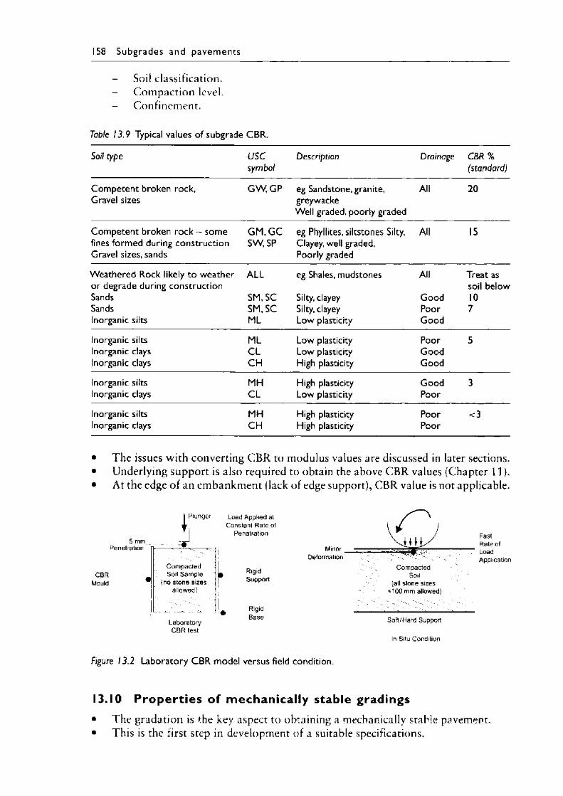
158 Subgrades and pavem ents
- Soil classification.- Compaction level.- Confinement.
Table 13.9 Typical values of subgrade CBR .
Soil type USCsymbol
Description Drainage CBR % (standard)
Competent broken rock, Gravel sizes
GW , GP eg Sandstone, granite, greywackeWell graded, poorly graded
All 20
Competent broken rock - some fines formed during construction Gravel sizes, sands
GM, G C SW ,SP
eg Phyllites, siltstones Silty, Clayey, well graded,Poorly graded
All 15
Weathered Rock likely to weather or degrade during construction Sands SandsInorganic silts
A LL
SM, SC SM .SC ML
eg Shales, mudstones
Silty, clayey Silty, clayey Low plasticity
All
GoodPoorGood
Treat as soil below 10 7
Inorganic silts Inorganic clays Inorganic clays
MLC LC H
Low plasticity Low plasticity High plasticity
PoorGoodGood
5
Inorganic silts Inorganic clays
MHC L
High plasticity Low plasticity
GoodPoor
3
Inorganic silts Inorganic clays
MHCH
High plasticity High plasticity
PoorPoor
<3
• The issues with converting C B R to modulus values are discussed in later sections.• Underlying support is also required to obtain the above C B R values (Chapter 11).• At the edge o f an embankment (lack of edge support), CBR value is not applicable.
C B RMould
Laboratory C B R test
Load Applied at Constant R ate of
Penatration
RigidSupport
RigidB a se
Com pactedSoil
(all stone s izes : 100 mm allowed)
Soft/Hard Support
In Situ Condition
Figure 13.2 Laboratory CBR model versus field condition.
I3.I0 P ro p ert ie s of m echanica l ly stable gradings• The gradation is the key aspect to obtaining a mechanically stable pavement.• This is the first step in development of a suitable specifications.
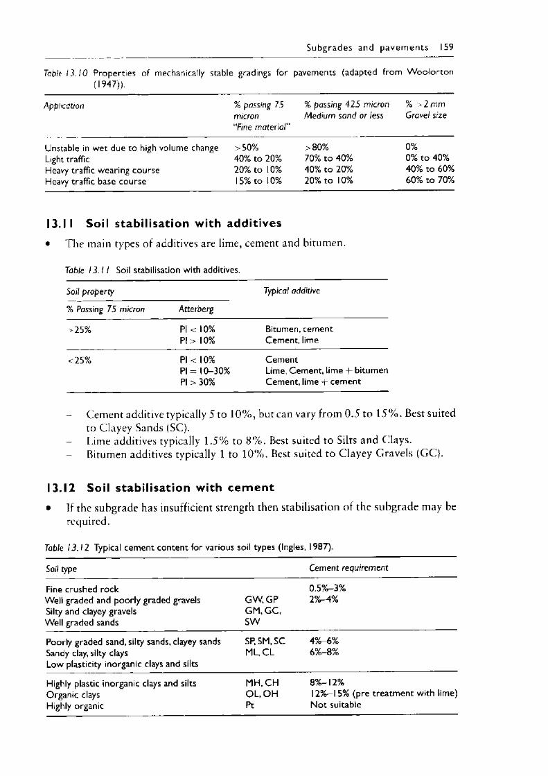
Subg rades and p a v e m e n ts 159
Table 13.10 Properties of mechanically stable gradings for pavements (adapted from Woolorton (1947)).
Application % passing 75 micron‘Tine material”
% passing 425 micron Medium sand or less
% >2 mm Gravel size
Unstable in wet due to high volume change >50% >80% 0%Light traffic 40% to 20% 70% to 40% 0% to 40%Heavy traffic wearing course 20% to 10% 40% to 20% 40% to 60%Heavy traffic base course 15% to 10% 20% to 10% 60% to 70%
I 3 J I Soil stabil isation with additives• The main types of additives are lime, cement and bitumen.
Table 13 .11 Soil stabilisation with additives.
Soil property Typical additive
% Passing 75 micron Atterberg
>25% PI < 10% Bitumen, cementPI > 10% Cement, lime
<25% PI < 10% CementP l= 10-30% Lime, Cement, lime -1- bitumenPI > 30% Cement, lime + cement
- Cement additive typically 5 to 1 0 % , but can vary from 0.5 to 1 5 % . Best suited to Clayey Sands (SC).Lime additives typically 1 .5% to 8 % . Best suited to Silts and Clays.
- Bitumen additives typically 1 to 1 0 % . Best suited to Clayey Gravels (GC).
13.12 Soil stabil isation with cem en t• If the subgrade has insufficient strength then stabilisation of the subgrade may be
required.
Table 13.12 Typical cement content for various soil types (Ingles, 1987).
Soil type Cement requirement
Fine crushed rock 0.5%-3%Well graded and poorly graded gravels G W ,G P 2%-4%Silty and clayey gravels GM, G C ,Well graded sands SW
Poorly graded sand, silty sands, clayey sands SP,SM,SC 4%-6%Sandy clay, silty clays ML, C L 6%-8%Low plasticity inorganic clays and silts
Highly plastic inorganic clays and silts MH, CH 8 % -12%Organic clays O L, OH 12%— 15% (pre treatment with lime)Highly organic Pt Not suitable
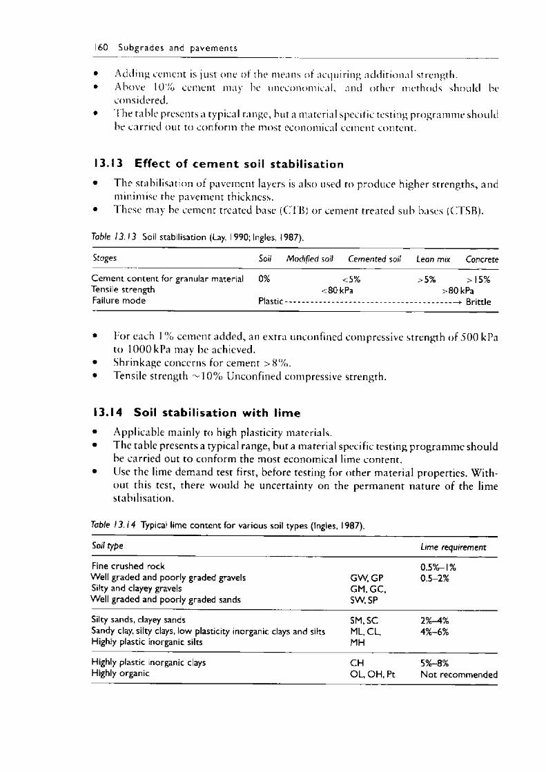
• Adding cement is just one of the means of acquiring additional strength.• Above 10% cement may be uneconomical, and other methods should be
considered.• 1 he table presents a typical range, but a material specific testing programme should
be carried out to conform the most economical cement content.
13.13 Effect of cem ent soil stabilisation• The stabilisation of pavement layers is also used to produce higher strengths, and
minimise the pavement thickness.• These may be cement treated base (CTB) or cement treated sub bases (CTSB).
160 Subgrades and pavem ents
Table 13.13 Soil stabilisation (Lay, I 990; Ingles, 1987).
Stages Soil Modified soil Cemented soil Lean mix Concrete
Cem ent content for granular material 0% <5% >5% >15%Tensile strength <80 kPa >80 kPaFailure mode ...................—» Brittle
• For each 1% cement added, an extra unconfined compressive strength of 5 0 0 kPa to lOOOkPa may be achieved.
• Shrinkage concerns for cement > 8 % .• Tensile strength ~ 1 0 % Unconfined compressive strength.
13.14 Soil stabil isation with lime• Applicable mainly to high plasticity materials.• The table presents a typical range, but a material specific testing programme should
be carried out to conform the most economical lime content.• Use the lime demand test first, before testing for other material properties. With
out this test, there would be uncertainty on the permanent nature of the lime stabilisation.
Table 13.14 Typical lime content for various soil types (Ingles, 1987).
Soil type Lime requirement
Fine crushed rock 0.5%-1%Well graded and poorly graded gravels G W .G P 0.5-2%Silty and clayey gravels G M .G C ,Well graded and poorly graded sands SW ,SP
Silty sands, clayey sands SM, SC 2%-4%Sandy clay, silty clays, low plasticity inorganic clays and silts ML, CL, 4%-6%Highly plastic inorganic silts MH
Highly plastic inorganic clays Highly organic
CHO L, OH, Pt
5%-8%Not recommended
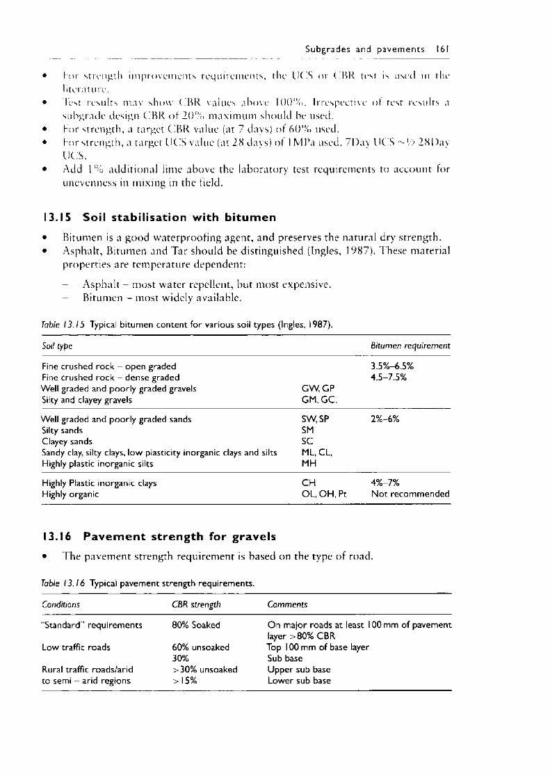
Subgrades and p avem ents 161
• l o r strength improvements requirements, the IK 'S or CBR test is used in the literature.
• Test results may show CBR values above 100%. Irrespective of test results a subgrade design C BR of 2 0 % maximum should be used.
• l o r strength, a target CBR value (at 7 days) of 6 0 % used.• lo r strength, a target UC'S value (at 28 days) of I MPa used. 7l)ay UCS Vi 28I)ay
IJCS.• Add 1% additional lime above the laboratory test requirements to account for
unevenness in mixing in the field.
13.15 Soil stabil isation with bitumen• Bitumen is a good waterproofing agent, and preserves the natural dry strength.• Asphalt, Bitumen and Tar should be distinguished (Ingles, 1987). These material
properties are temperature dependent:
Asphalt - most water repellent, but most expensive.- Bitumen - most widely available.
Table 13.15 Typical bitumen content for various soil types (Ingles, 1987).
Soil type Bitumen requirement
Fine crushed rock - open graded Fine crushed rock - dense graded Well graded and poorly graded gravels Silty and clayey gravels
G W ,G P GM, G C ,
3.5%—6.5% 4.5-7.5%
Well graded and poorly graded sands Silty sands Clayey sandsSandy clay, silty clays, low plasticity inorganic clays and silts Highly plastic inorganic silts
SW,SPSMSCML. CL, MH
2%-6%
Highly Plastic inorganic clays CH 4%-7%Highly organic O L, O H , Pt Not recommended
13.16 P avem en t strength for gravels• The pavement strength requirement is based on the type of road.
Table 13.16 Typical pavement strength requirements.
Conditions CBR strength Comments
“Standard” requirements 80% Soaked On major roads at least 100 mm of pavement layer >80% CBR
Low traffic roads 60% unsoaked Top 100 mm of base layer30% Sub base
Rural traffic roads/arid >30% unsoaked Upper sub baseto semi - arid regions > 15% Lower sub base
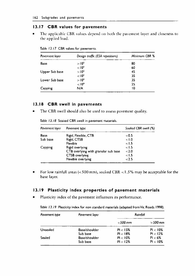
162 Subgrades and pavem ents
13.17 C B R values for pavem ents• The applicable CBR values depend on both the pavement layer and closeness to
the applied load.
Table 13 .17 CBR values for pavements.
Pavement layer Design traffic (ESA repetitions) Minimum CBR %
Base > I0 6 80< I0 6 60
Upper Sub base > I0 6 45< I0 6 35
Lower Sub base >10" 35< I0 6 25
Capping N/A 10
13.18 C B R swell in pavem ents• The C BR swell should also be used to assess pavement quality.
Table 13.18 Soaked CBR swell in pavement materials.
Pavement layer Pavement type Soaked CBR swell (%)
Base Rigid, Flexible, C T B <0.5Sub base Rigid, CTSB <1.0
Flexible <1.5Capping Rigid overlying <1.5
C TB overlying with granular sub base <2.0CTSB overlying <1.5Flexible overlying <2.5
• For low rainfall areas ( < 5 0 0 mm), soaked C BR < 1 . 5 % may be acceptable for the base layer.
13.19 Plastic ity index propert ies of pavem ent m ater ia ls• Plasticity index of the pavement influences its performance.
Table 13.19 Plasticity index for non standard materials (adapted from Vic Roads 1998).
Pavement type Pavement layer Rainfall
< 500 mm > 5 00 mm
Unsealed Base/shoulder PI < 1 5% PI < 10%Sub base PI < 18% PI < 12%
Sealed Base/shoulder PI < 10% PI < 6%Sub base PI < 12% PI < 10%
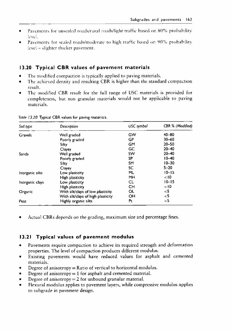
Subgrades and p avem ents 163
• Pavements for unsealed roads/rural roads/light traffic based on 8 0 % probability level.
• Pavements for sealed roads/moderate to high traffic based on 9 0 % probability level - slighter thicker pavement.
13.20 Typica l C B R values of pavement materia ls• The modified compaction is typically applied to paving materials.• The achieved density and resulting CBR is higher than the standard compaction
result.• The modified C BR result for the full range of USC materials is provided for
completeness, but non granular materials would not be applicable to paving materials.
Table 13 .20 Typical CBR values for paving materials.
Soil type Description USC symbol CBR % (Modified)
Gravels Well graded G W 40-80Poorly graded GP 30-60Silty GM 20-50Clayey G C 20-40
Sands Well graded SW 20—40Poorly graded SP 10-40Silty SM 10-30Clayey SC 5-20
Inorganic silts Low plasticity ML 10-15High plasticity MH <10
Inorganic clays Low plasticity C L 10-15High plasticity CH <10
Organic W ith silt/clays of low plasticity O L <5W ith silt/clays of high plasticity O H <5
Peat Highly organic silts Pt <5
• Actual C BR s depends on the grading, maximum size and percentage fines.
13.21 Typica l values of pavem ent modulus• Pavements require compaction to achieve its required strength and deformation
properties. The level of compaction produces different modulus.• Existing pavements would have reduced values for asphalt and cemented
materials.• Degree of anisotropy = Ratio of vertical to horizontal modulus.• Degree of anisotropy = 1 for asphalt and cemented material.• Degree o f anisotropy = 2 for unbound granular material.• Flexural modulus applies to pavement layers, while compressive modulus applies
to subgrade in pavement design.
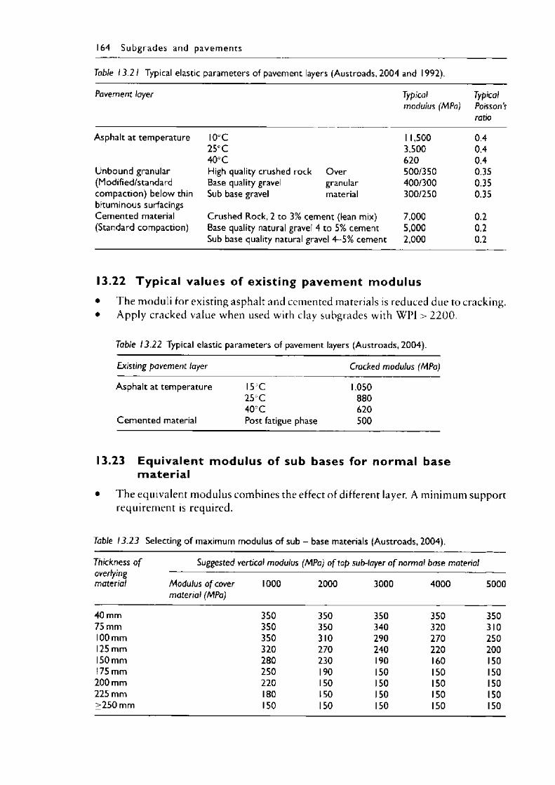
164 Subg rades and pavem ents
Table 13 .2 1 Typical elastic parameters of pavement layers (Austroads, 2004 and 1992).
Pavement layer Typicalmodulus (MPa)
TypicalPoissonsratio
Asphalt at temperature IO C 1 1,500 0.425 C 3,500 0.440 C 620 0.4
Unbound granular High quality crushed rock Over 500/350 0.35(Modified/standard Base quality gravel granular 400/300 0.35compaction) below thin Sub base gravel material 300/250 0.35bituminous surfacingsCemented material Crushed Rock, 2 to 3% cement (lean mix) 7,000 0.2(Standard compaction) Base quality natural gravel 4 to 5% cement 5,000 0.2
Sub base quality natural gravel 4-5% cement 2,000 0.2
13.22 Typica l values of existing pavement modulus• The moduli for existing asphalt and cemented materials is reduced due to cracking.• Apply cracked value when used with clay subgrades with WPI > 2200 .
Table 13 .22 Typical elastic parameters of pavement layers (Austroads, 2004).
Existing pavement layer Cracked modulus (MPa)
Asphalt at temperature 15 C 1,05025 C 88040 C 620
Cemented material Post fatigue phase 500
13.23 Equivalent modulus of sub bases for normal base materia l
• The equivalent modulus combines the effect of different layer. A minimum support requirement is required.
Table 13.23 Selecting of maximum modulus of sub - base materials (Austroads, 2004).
Thickness o f Suggested vertical modulus (MPa) o f top sub-layer o f normal base materialoverlying ~-----------------------------------------------------------------------------------------material Modu/us o f cover
material (MPa)1000 2000 3000 4000 5000
40 mm 350 350 350 350 35075 mm 350 350 340 320 310100 mm 350 310 290 270 250125 mm 320 270 240 220 200150 mm 280 230 190 160 150175 mm 250 190 150 150 150200 mm 220 150 150 150 150225 mm 180 150 150 150 150>250 mm 150 150 150 150 150
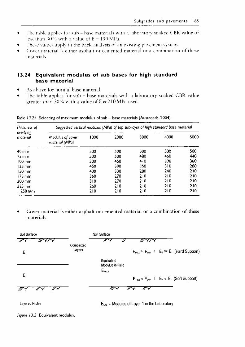
Subgrades and p avem ents 165
• The table applies for sub - base materials with a laboratory soaked CBR value of less than 3 0 % with a value of K — 150 MPa.
• These values apply in the back-analysis of an existing pavement system.• Cover material is either asphalt or cemented material or a combination of these
materials.
13.24 Equivalent modulus of sub bases for high standard base materia l
• As above for normal base material.• The table applies for sub - base materials with a laboratory soaked C B R value
greater than 3 0 % with a value of E = 2 1 0 MPa used.
Table 13.24 Selecting of maximum modulus of sub - base materials (Austroads, 2004).
Thickness o foverlyingmaterial
Suggested vertical modulus (MPa) o f top sub-layer o f high standard base material
Modulus o f cover material (MPa)
1000 2000 3000 4000 5000
40 mm 500 500 500 500 50075 mm 500 500 480 460 440100 mm 500 450 410 390 360125 mm 450 390 350 310 280150 mm 400 330 280 240 210175 mm 360 270 210 210 210200 mm 310 270 210 210 210225 mm 260 210 210 210 210>250 mm 210 210 210 210 210
Cover material is either asphalt or cemented material or a combination of these materials.
Soil Surface Soil SurfaceT 9— //v /v ------- ---------------------------------^9 7 # y /v
CompactedE , Layers E f,eld> E * . if E ; » E , (Hard Support)
Equivalent Modulus in FieldE fiELD
EfiEID< ElAB if E2 < E, (Soft Support)
7T7---- 7 7— ^ 7--- --------- -------- ^ 7— 7*7
Layered Profile E LAb = Modulus of Layer 1 in the Laboratory
Figure 13.3 Equivalent modulus.
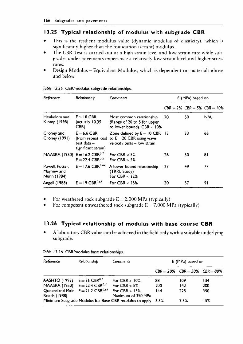
166 Subgrades and pavem ents
13.25 Typ ica l re la t ionsh ip of m odulus with su b g ra d e C B R• This is the resilient modulus value (dynamic modulus of elasticity), which is
significantly higher than the foundation (secant) modulus.• The CBR Test is carried out at a high strain level and low strain rate while sub-
grades under pavements experience a relatively low strain level and higher stress rates.
• Design Modulus = Equivalent Modulus, which is dependent on materials above and below.
Table 13.25 CBR/modulus subgrade relationships.
Reference Relationship Comments
CBR
E (MPa) based
= 2% CBR = 5%
on
CBR= 10%
Heukelom and Klomp (1998)
E ~ 10 CBR (actually 10.35 CBR)
Most common relationship (Range of 20 to 5 for upper to lower bound). CBR < 10%
20 50 N/A
Croney and Croney (1991)
E = 6.6 CBR (from repeat load test data - significant strain)
Zone defined by E = 10 CBR to E = 20 CBR using wave velocity tests - low strain
13 33 66
N AASRA (1950) E = 16.2 C B R 0 7 E = 22.4 C B R 0 s
For CBR < 5% For CBR > 5%
26 50 81
Powell, Potter, Mayhew and Nunn (1984)
E = 17.6 CB R 0 64 A lower bound relationship (TRRL Study)For CBR < 12%
27 49 77
Angell (1988) E = 19 CB R 0 68 For CB R < 15% 30 57 91
• For weathered rock subgrade E = 2 ,0 0 0 MPa (typically)• For competent unweathered rock subgrade E = 7 ,0 0 0 MPa (typically)
13.26 Typical relationship of modulus with base course C B R• A laboratory CBR value can be achieved in the field only with a suitable underlying
subgrade.
Table 13.26 CBR/modulus base relationships.
Reference Relationship Comments E (MPa) based on
CBR = 20% C B R = 50% C BR= 80%
AASH TO (1993) E = 36 C B R 0 5 For CBR > 10% 88 109 134N AASRA (1950) E = 22.4 C B R 0-5 For CBR > 5% 100 142 200Queensland Main E = 21.2 C B R 0 64 For CBR > 15% 144 225 350Roads (1988) Maximum of 350 MPaMinimum Subgrade Modulus for Base CBR modulus to apply 3.5% 7.5% 15%
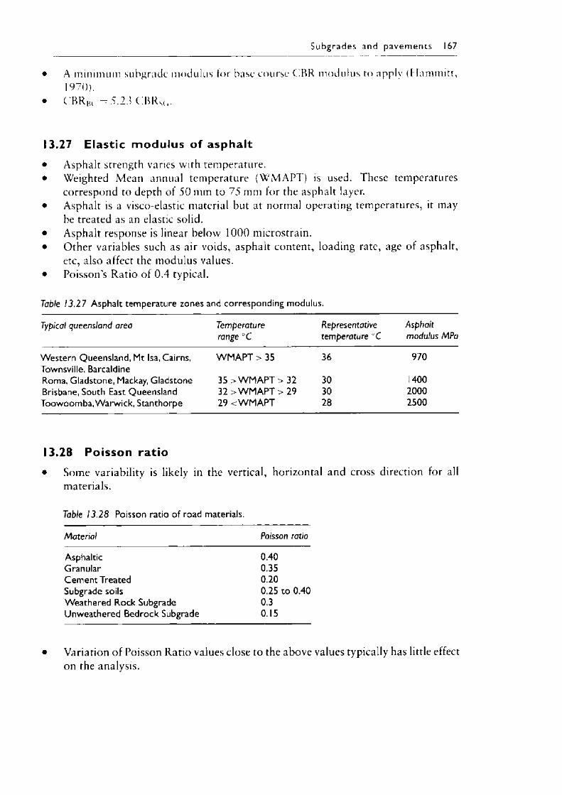
Subgrades and pavem ents 167
• A minimum subgrade modulus for base course CBR modulus to apply (Hammitt, 1970).
• CBR|« = 5 . 2 3 C B R S(l.
13.27 Elast ic modulus of asphalt• Asphalt strength varies with temperature.• Weighted Mean annual temperature (WMAPT) is used. These temperatures
correspond to depth of 50 mm to 75 mm for the asphalt layer.• Asphalt is a visco-elastic material but at normal operating temperatures, it may
be treated as an elastic solid.• Asphalt response is linear below 1000 microstrain.• Other variables such as air voids, asphalt content, loading rate, age of asphalt,
etc, also affect the modulus values.• Poisson’s Ratio of 0.4 typical.
Table 13 .27 Asphalt temperature zones and corresponding modulus.
Typical queensland area Temperature range °C
Representative temperature °C
Asphalt modulus MPa
Western Queensland, Mt Isa, Cairns, Townsville, Barcaldine
W M APT > 35 36 970
Roma, Gladstone, Mackay, Gladstone 35 > W M APT > 32 30 1400Brisbane, South East Queensland 32 > W M APT > 29 30 2000Toowoomba, Warwick, Stanthorpe 29 < W M APT 28 2500
13.28 Poisson rat io• Some variability is likely in the vertical, horizontal and cross direction for all
materials.
Table 13.28 Poisson ratio of road materials.
Material Poisson ratio
Asphaltic 0.40Granular 0.35Cement Treated 0.20Subgrade soils 0.25 to 0.40Weathered Rock Subgrade 0.3Unweathered Bedrock Subgrade 0.15
• Variation of Poisson Ratio values dose to the above values typically has little effect on the analysis.

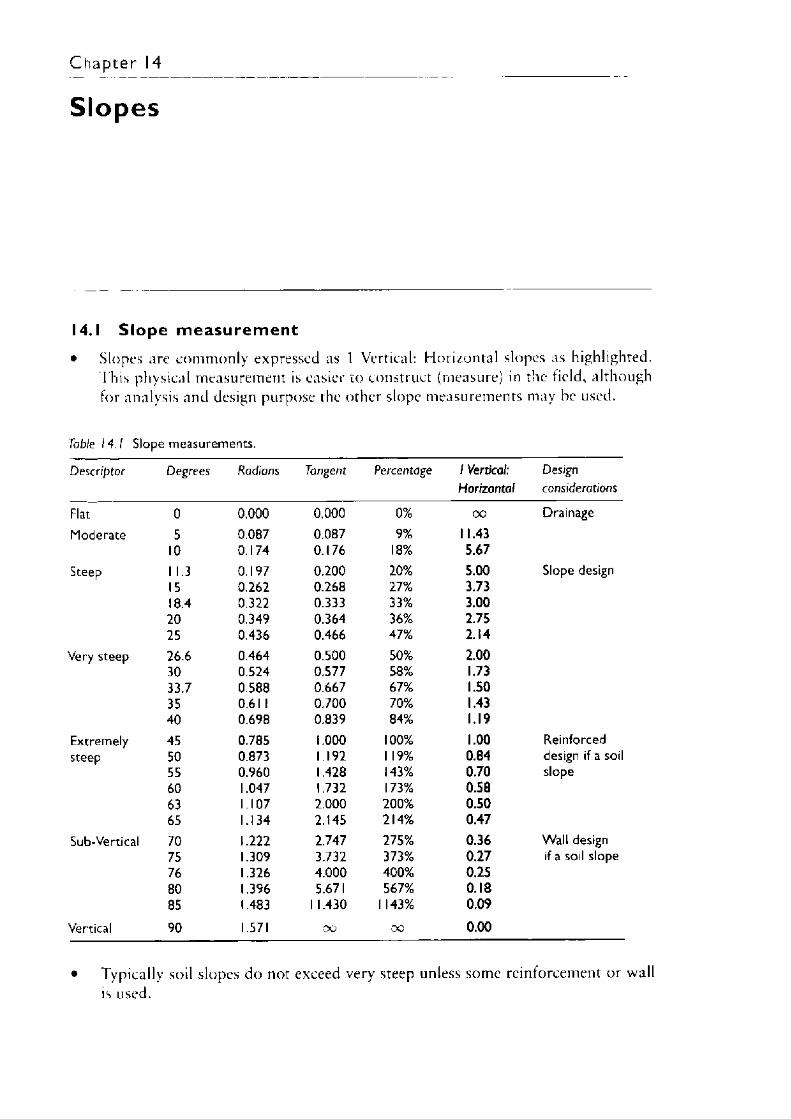
Chapter 14
Slopes
14.1 S lop e m e a s u re m e n t• Slopes are commonly expressed as 1 Vertical: Horizontal slopes as highlighted.
This physical measurement is easier to construct (measure) in the field, although for analysis and design purpose the other slope measurements may he used.
Table 14.1 Slope measurements.
Descriptor Degrees Radians Tangent Percentage 1 Vertical: Horizontal
Designconsiderations
Flat 0 0.000 0.000 0% 00 DrainageModerate 5 0.087 0.087 9% 11.43
10 0.174 0.176 18% 5.67Steep 1 1.3 0.197 0.200 20% 5.00 Slope design
15 0.262 0.268 27% 3.7318.4 0.322 0.333 33% 3.0020 0.349 0.364 36% 2.7525 0.436 0.466 47% 2.14
Very steep 26.6 0.464 0.500 50% 2.0030 0.524 0.577 58% 1.7333.7 0.588 0.667 67% 1.5035 0.61 1 0.700 70% 1.4340 0.698 0.839 84% 1.19
Extremely 45 0.785 1.000 100% 1.00 Reinforcedsteep 50 0.873 1.192 1 19% 0.84 design if a soil
55 0.960 1.428 143% 0.70 slope60 1.047 1.732 173% 0.5863 1.107 2.000 200% 0.5065 1.134 2.145 214% 0.47
Sub-Vertical 70 1.222 2.747 275% 0.36 Wall design75 1.309 3.732 373% 0.27 if a soil slope76 1.326 4.000 400% 0.2580 1.396 5.671 567% 0.1885 1.483 1 1.430 1 143% 0.09
Vertical 90 1.571 00 oo 0.00
• Typically soil slopes do not exceed very steep unless some reinforcement or wall is used.
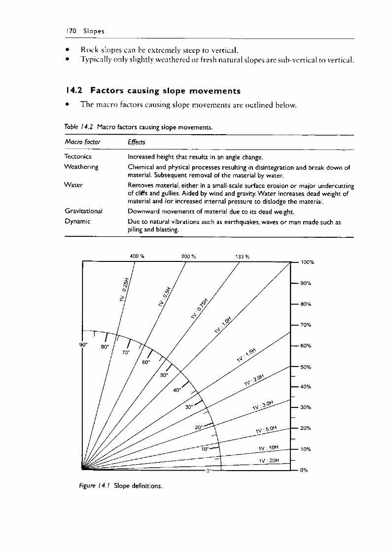
170 S lo pes
• Rock slopes can be extremely steep to vertical.• Typically only slightly weathered or fresh natural slopes are sub-vertical to vertical.
14.2 Fac to rs causing slope m ovem ents• The macro factors causing slope movements are outlined below.
Table 14.2 Macro factors causing slope movements.
Macro factor Effects
Tectonics Increased height that results in an angle change.Weathering Chemical and physical processes resulting in disintegration and break down of
material. Subsequent removal of the material by water.W ater Removes material, either in a small-scale surface erosion or major undercutting
of cliffs and gullies. Aided by wind and gravity. W ater Increases dead weight of material and /or increased internal pressure to dislodge the material.
Gravitational Downward movements of material due to its dead weight.Dynamic Due to natural vibrations such as earthquakes, waves or man made such as
piling and blasting.
400 % 200 % 133 %
Figure 14.1 Slope definitions.
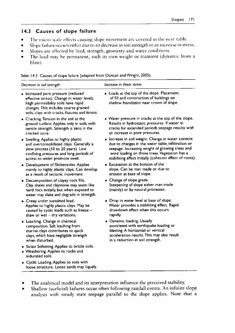
S lo p es 171
14.3 Causes of slope failure• The micro scale effects causing slope movement are covered in the next table.• Slope failure occurs either due to an decrease in soil strength or an increase in stress.• Slopes are affected by load, strength, geometry and water conditions.• The load may be permanent, such its own weight or transient (dynamic from a
blast).
Table 14.3 Causes of slope failure (adapted from Duncan and Wright, 2005).
Decrease in soil strength Increase in shear stress
• Increased pore pressure (reduced effective stress). Change in water levels. High permeability soils have rapid changes. This includes coarse grained soils, clays with cracks, fissures and lenses.
• Cracking. Tension in the soil at the ground surface. Applies only in soils with tensile strength. Strength is zero in the cracked zone.
• Swelling. Applies to highly plasticand overconsolidated clays. Generally a slow process (10 to 20 years). Low confining pressures and long periods of access to water promote swell.
• Development of Slickensides. Applies mainly to highly plastic clays. Can develop as a result of tectonic movement.
• Decomposition of clayey rock fills.Clay shales and claystone may seem like hard rock initially, but when exposed to water may slake and degrade in strength.
• Creep under sustained load.Applies to highly plastic clays. May be caused by cyclic loads such as freeze - thaw or wet - dry variations.
• Leaching. Change in chemical composition. Salt leaching from marine clays contributes to quick clays, which have negligible strength when disturbed.
• Strain Softening. Applies to brittle soils.• Weathering. Applies to rocks and
indurated soils.• Cyclic Loading. Applies to soils with
loose structure. Loose sands may liquefy.
Loads at the top of the slope. Placement of fill and construction of buildings on
shallow foundation near crown of slope.
• W ater pressure in cracks at the top of the slope. Results in hydrostatic pressures. If water in cracks for extended periods seepage results with an increase in pore pressures.
• Increase in soil weight. Change in water content due to changes in the water table, infiltration or seepage. Increasing weight of growing trees and wind loading on those trees. Vegetation has a
stabilising effect initially (cohesion effect of roots).• Excavation at the bottom of the
slope. Can be man made or due to erosion at base of slope.
• Change of slope grade.Steepening of slope either man made (mainly) or by natural processes.
• Drop in water level at base of slope.Water provides a stabilising effect. Rapid drawdown effect when this occurs rapidly.
• Dynamic loading. Usually associated with earthquake loading or blasting. A horizontal or vertical acceleration results. This may also result in a reduction in soil strength.
• The analytical model and its interpretation influence the perceived stability.• Shallow (surficial) failures occur often following rainfall events. An infinite slope
analysis with steady state seepage parallel to the slope applies. Note that a
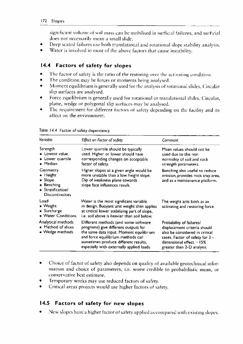
172 S lopes
significant volume of soil mass can he mobilised in surficial failures, and surficial does not necessarily mean a small slide.
• Deep seated failures use both translational and rotational slope stability analysis.• Water is involved in most of the above factors that cause instability.
14.4 Factors of safety for slopes• The factor of safety is the ratio of the restoring over the activating condition.• The condition may be forces or moments being analysed.• Mom ent equilibrium is generally used for the analysis of rotational slides. Circular
slip surfaces are analysed.• Force equilibrium is generally used for rotational or translational slides. Circular,
plane, wedge or polygonal slip surfaces may be analysed.• The requirement for different factors of safety depending on the facility and its
affect on the environment.
Table 14.4 Factor of safety dependency.
Variable Effect on Factor o f safety Comment
Strength• Lowest value• Lower quartile• MedianGeometry• Height• Slope• Benching• Stratification/
DiscontinuitiesLoad• Weight• Surcharge• W ater ConditionsAnalytical methods• Method of slices• Wedge methods
Lower quartile should be typically used. Higher or lower should have corresponding changes on acceptable factor of safety.Higher slopes at a given angle would be more unstable than a low height slope. Dip of weakness plane towards slope face influences result.
Water is the most significant variable in design. Buoyant unit weight then applies at critical lower stabilizing part of slope, i.e. soil above is heavier than soil below.Different methods (and some software programs) give different outputs for the same data input. Moment equilibrium and force equilibrium methods can sometimes produce different results, especially with externally applied loads.
Mean values should not be used due to the non normality of soil and rock strength parameters.Benching also useful to reduce erosion, provides rock trap area, and as a maintenance platform.
The weight acts both as an activating and restoring force.
Probability of failures/ displacement criteria should also be considered in critical cases. Factor of safety for 3 - dimensional effect ~ I5% greater than 2-D analysis.
• Choice of factor of safety also depends on quality of available geotechnical information and choice of parameters, i.e. worst credible to probabilistic mean, or conservative best estimate.
• Temporary works may use reduced factors of safety.• Critical areas projects would use higher factors of safety.
14.5 Fac to rs of safety for new slopes• New slopes have a higher factor of safety applied as compared with existing slopes.
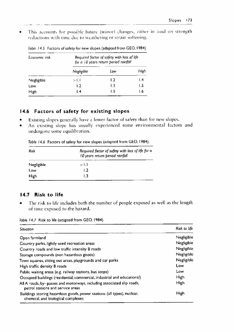
S lopes 173
• This accounts for possible future (minor) changes, either in load on strength reductions with time due to weathering or strain softening.
Table 14.5 Factors of safety for new slopes (adapted from G EO , 1984).
Economic risk Required factor o f safety with loss o f life for a 10 years return period rainfall
Negligible Low High
Negligible >1.1 1.2 1.4Low 1.2 1.3 1.5High 1.4 1.5 1.6
14.6 Factors of safety for existing slopes• Existing slopes generally have a lower factor of safety than for new slopes.• An existing slope has usually experienced some environmental factors and
undergone some equilibration.
Table 14.6 Factors of safety for new slopes (adapted from GEO, 1984).
Risk Required factor o f safety with loss o f life for a 10 years return period rainfall
Negligible >1.1Low 1.2High 1.3
14.7 Risk to life• The risk to life includes both the number of people exposed as well as the length
of time exposed to the hazard.
Table 14.7 Risk to life (adapted from GEO, 1984).
Situation Risk to life
Open farmland NegligibleCountry parks, lightly used recreation areas NegligibleCountry roads and low traffic intensity B roads NegligibleStorage compounds (non hazardous goods) NegligibleTown squares, sitting out areas, playgrounds and car parks NegligibleHigh traffic density B roads LowPublic waiting areas (e.g. railway stations, bus stops) LowOccupied buildings (residential, commercial, industrial and educational) HighAll A roads, by- passes and motorways, including associated slip roads,
petrol stations and service areasHigh
Buildings storing hazardous goods, power stations (all types), nuclear, Highchemical, and biological complexes
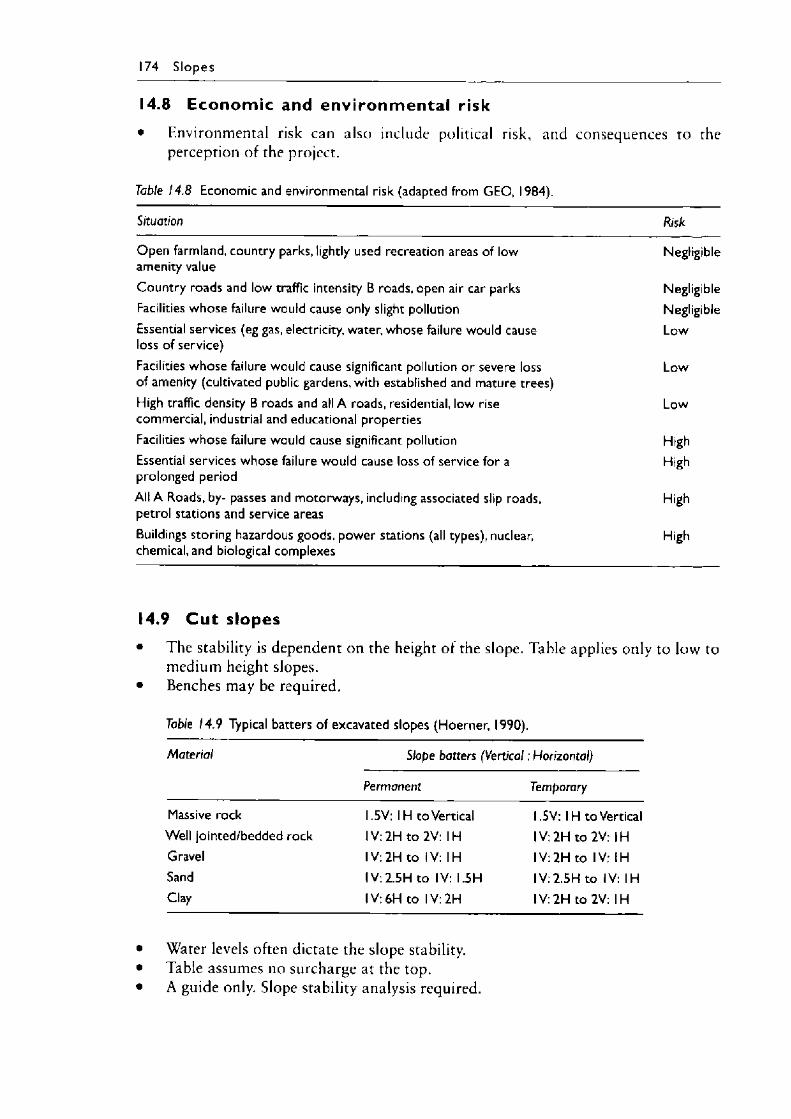
174 S lopes
14.8 Econ om ic and environmental risk• Environmental risk can also include political risk, and
perception of the project.
Table 14.8 Economic and environmental risk (adapted from GEO, 1984).
consequences to the
Situation Risk
Open farmland, country parks, lightly used recreation areas of low amenity value
Negligible
Country roads and low traffic intensity B roads, open air car parks NegligibleFacilities whose failure would cause only slight pollution NegligibleEssential services (eg gas, electricity, water, whose failure would cause loss of service)
Low
Facilities whose failure would cause significant pollution or severe loss of amenity (cultivated public gardens, with established and mature trees)
Low
High traffic density B roads and all A roads, residential, low rise commercial, industrial and educational properties
Low
Facilities whose failure would cause significant pollution HighEssential services whose failure would cause loss of service for a prolonged period
High
All A Roads, by- passes and motorways, including associated slip roads, petrol stations and service areas
High
Buildings storing hazardous goods, power stations (all types), nuclear, chemical, and biological complexes
High
14.9 C u t slopes• The stability is dependent on the height of the slope. Table applies only to low to
medium height slopes.• Benches may be required.
Table 14.9 Typical batters of excavated slopes (Hoerner, 1990).
Material Slope batters (Vertical: Horizontal)
Permanent Temporary
Massive rock 1.5V: 1H to Vertical 1.5V: 1H to VerticalWell jointed/bedded rock IV: 2H to 2V: IH IV: 2H to 2V: IHGravel IV: 2H to IV: IH IV: 2H to IV: IHSand IV:2.5H to IV: I.5H IV:2.5H to IV: IHClay IV: 6H to IV: 2H IV :2H to 2V: IH
• Water levels often dictate the slope stability.• Table assumes no surcharge at the top.• A guide only. Slope stability analysis required.
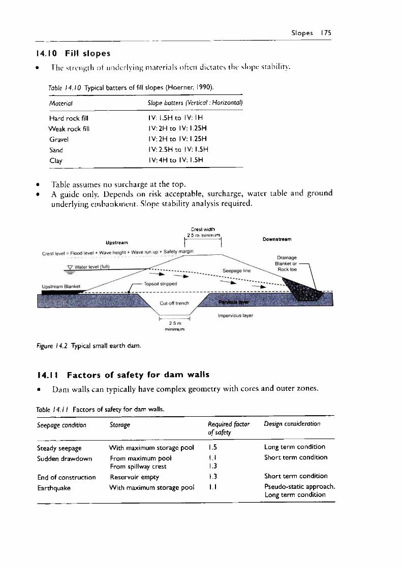
I 4 .1 0 Fill slopes• The strength of underlying materials often dictates the slope stability.
Slopes 175
Table 14.10 Typical batters of fill slopes (Hoerner, 1990).
Material Slope batters (Vertical: Horizontal)
Hard rock fill IV: I.5H to IV: IHWeak rock fill IV: 2H to IV: I.25HGravel IV: 2H to IV: I.25HSand 1V: 2.5H to IV: I.5HClay IV :4H to IV: I.5H
• Table assumes no surcharge at the top.• A guide only. Depends on risk acceptable, surcharge, water table and ground
underlying embankment. Slope stability analysis required.
Crest width 2 5 m minimum
------------------------—H D ow nstreamU pstream
minimum
Figure 14.2 Typical small earth dam.
14.1 I Factors of safety for dam walls• Dam walls can typically have complex geometry with cores and outer zones.
Table 14.11 Factors of safety for dam walls.
Seepage condition Storage Required factor o f safety
Design consideration
Steady seepage W ith maximum storage pool 1.5 Long term conditionSudden drawdown From maximum pool
From spillway crestl.l1.3
Short term condition
End of construction Reservoir empty 1.3 Short term conditionEarthquake With maximum storage pool l.l Pseudo-static approach.
Long term condition
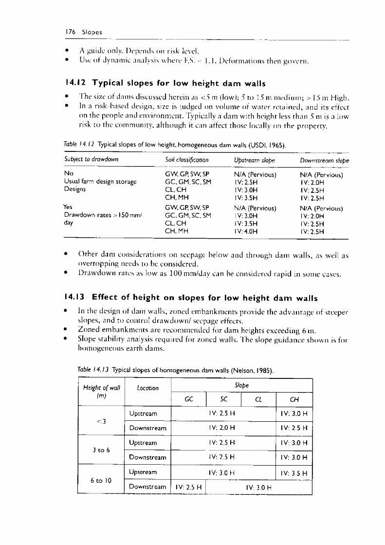
• A guide only. Depends on risk level.• Use of dynamic analysis where I .S. < 1.1. Deformations then govern.
14.12 Typical slopes for low height dam walls• I he size of dams discussed herein as <5 m (low); 5 to 1 5 m medium; > 1 5 m High.• In a risk-based design, size is judged on volume of water retained, and its effect
on the people and environment. Typically a dam with height less than 5 m is a low risk to the community, although it can affect those locally on the property.
Table 14.12 Typical slopes of low height, homogeneous dam walls (USDI, 1965).
176 Slopes
Subject to drawdown Soil classification Upstream slope Downstream slope
No G W .G P.SW .SP N/A (Pervious) N/A (Pervious)Usual farm design storage G C , GM, SC, SM IV: 2.5H 1V: 2.OHDesigns CL, CH IV: 3.OH 1V: 2.5H
C H , MH IV: 3.5H 1V: 2.5HYes GW , GP, SW, SP N/A (Pervious) N/A (Pervious)Drawdown rates > 150 mm/ G C , GM, SC, SM IV: 3.OH IV: 2.OHday C L , CH 1V: 3.5H IV: 2.5H
C H , MH 1V: 4.OH IV: 2.5H
• Other dam considerations on seepage below and through dam walls, as well as overtopping needs to be considered.
• Drawdown rates as low as 100 mm/day can be considered rapid in some cases.
14.13 Effect of height on slopes for low height dam walls• In the design of dam walls, zoned embankments provide the advantage of steeper
slopes, and to control drawdown/ seepage effects.• Zoned embankments are recommended for dam heights exceeding 6 m.• Slope stability analysis required for zoned walls. I he slope guidance shown is for
homogeneous earth dams.
Table 14.13 Typical slopes of homogeneous dam walls (Nelson, 1985).
Height o f wall (m)
Location Slope
GC SC CL CH
<3Upstream IV: 2.5 H IV: 3.0 H
Downstream IV: 2.0 H IV: 2.5 H
3 to 6Upstream IV: 2.5 H IV: 3.0 H
Downstream IV: 2.5 H IV: 3.0 H
6 to 10__
Upstream IV: 3.0 H IV: 3.5 H
Downstream IV: 2.5 H IV: 3.0 H
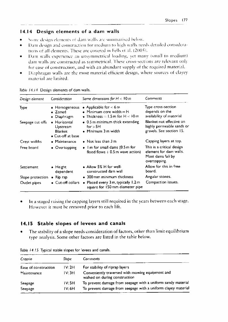
• Some design elements of dam walls are summarised below.• Dam design and construction for medium to high walls needs detailed considera
tions of all elements. These are covered in Fells et al. (2005).• Dam walls experience an unsymmetrical loading, yet many (small to medium)
dam walls are constructed as symmetrical. These cross-sections are relevant onlyfor ease of construction, and with an abundant supply of the required material.
• Diaphragm walls are the most material efficient design, where sources of clayey material are limited.
Slopes 177
14.14 Design e l em en ts of a dam walls
Table 14.14 Design elements of dam walls.
Design element Consideration Some dimensions for H < 10 m Comments
Type 9 Homogeneous • Applicable for < 6 m Type cross-section• Zoned • Minimum core width = H depends on the• Diaphragm 9 Thickness - 1.5 m for H < 10 m availability of material.
Seepage cut offs • Horizontal • 0.5 m minimum thick extending Blanket not effective onUpstream for >5H highly permeable sands orBlanket • Minimum 3 m width gravels. See section 15.
• Cut-off at baseCrest widths • Maintenance • Not less than 3 m Capping layers at top.Free board • Overtopping • 1 m for small dams (0.5 m for
flood flows -f 0.5 m wave action)This is a critical design element for dam walls. Most dams fail by overtopping.
Settlement • Height • Allow 5% H for well- Allow for this in freedependent constructed dam wall board.
Slope protection • Rip rap • 300 mm minimum thickness Angular stones.Outlet pipes • Cut-off collars • Placed every 3 m, typically 1.2 m
square for 150 mm diameter pipeCompaction issues.
• In a staged raising the capping layers still required in the years between each stage. However it must be removed prior to each lift.
14.15 Stable slopes of levees and canals• The stability of a slope needs consideration of factors, other than limit equilibrium
type analysis. Some other factors are listed in the table below.
Table 14.15 Typical stable slopes for levees and canals.
Criteria Slope Comments
Ease of construction IV: 2H For stability of riprap layersMaintenance IV: 3H Conveniently traversed with mowing equipment and
walked on during constructionSeepage IV: 5H To prevent damage from seepage with a uniform sandy materialSeepage IV: 6H To prevent damage from seepage with a uniform clayey material
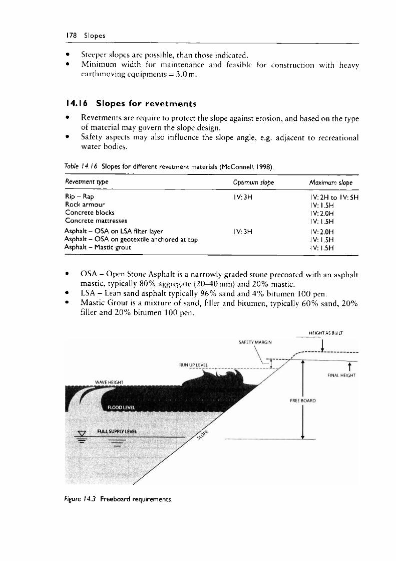
178 S lopes
• Steeper slopes are possible, than those indicated.• Minimum width for maintenance and feasible for construction with heavy
earthmoving equipments = 3 .0 m.
14.16 Slopes for revetm ents• Revetments are require to protect the slope against erosion, and based on the type
of material may govern the slope design.• Safety aspects may also influence the slope angle, e.g. adjacent to recreational
water bodies.
Table 14.16 Slopes for different revetment materials (McConnell, 1998).
Revetment type Optimum slope Maximum slope
Rip - Rap IV: 3H IV 2H to IV: 5HRock armour IV I.5HConcrete blocks IV 2.OHConcrete mattresses IV I.5HAsphalt - O SA on LSA filter layer IV: 3H IV 2.OHAsphalt - O SA on geotextile anchored at top IV I.5HAsphalt - Mastic grout IV I.5H
• OSA - Open Stone Asphalt is a narrowly graded stone precoated with an asphaltmastic, typically 8 0 % aggregate ( 2 0 - 4 0 mm) and 2 0 % mastic.
• LSA - Lean sand asphalt typically 9 6 % sand and 4 % bitumen 100 pen.• Mastic Grout is a mixture of sand, filler and bitumen, typically 6 0 % sand, 2 0 %
filler and 2 0 % bitumen 100 pen.
HEIGHT AS BUILT
Figure 14.3 Freeboard requirements.
S lo p es 179
14.17 C r e s t levels based on revetm ent type• T he crest levels are based principally on design wave heights (based on fetch, wind
and water depths).• Significant water depth = H s.• Other controlling factors are slope and revetment type.• The required freeboard is then based on consideration of all of the above factors.• Design wave height factored according to the next 2 tables.
Table 14.17 Design wave height, HD (McConnell, 1998).
Revetment type Crest configuration Design wave height, Ho
Concrete/Masonry 0.75 HsRockfill Surfaced road 1.0 HsEarthfill with reinforced downstream face Surfaced road l.l HsEarthfill with grass downstream face Surfaced road 1.2 Hs
Grass crest 1.3 HsAll embankment types - no still water or 1.67 Hs
wave surcharge carryover permitted
14.18 C r e s t levels based on revetm ent slope• The design wave height is factored according to the run-up factor x H D• The run-up factor is based on the dam slope provided in table below.
Table 14.18 Run-up factor based on slope (adapted from McConnell, 1998).
Dam slope Run-up factor
Maximum Intermediate Minimum(smooth slope) (rough stone or shallow rubble) (thick permeable rip-rap)
IV: 5H 1.0 0.85 0.65IV: 4H 1.25 1.05 0.8IV: 3H 1.7 1.35 1.05IV: 2.5H 1.95 1.55 1.2IV: 2H 2.2 1.75 1.35
• Different overtopping limit apply based on the access requirements, type ofstructure and land use immediately behind.
14.19 Stable slopes underwater• Slope stability analysis alone does not capture the stability of slope under water.• Slopes fully underwater tend to be stable at much flatter angles than indicated
by slope stability analysis.• This is due to the activity of the water and continuous erosion effects under water.
180 Slopes
Table 14.19 Typical slopes underwater (ICE, 1995).
Type o f material Description Slopes in still water Slopes in active water
Rock Nearly vertical Nearly vertical
Clay Stiff 45° IV: IH 45 IV IHFirm 35 IV: I.4H 30 IV I.7HSandy 25 IV: 2 .IH 15 IV 3.7 H
Sand Coarse 20 IV: 2.7H 10° IV 5.7HFine 15° IV: 3.7H 5° IV 1 I.4H
Silt Mud 10-1° IV: 5.7H to 57H <5 IV 1 1.4 H or less
14.20 Side slopes for canals in different materia ls• The side slopes in canals depends on the type of natural materials, and the canal
depth.• A canal that is 1.0 m in depth may have material that can have a 1V: 1 .OH slopes,
while at 2 .0 m depth a slope of IV: 2 .OH may be required.• The flow velocity in the canal may require revetment protection, and that may
govern the slope.
Table 14.20 Typical slopes for earthen canals in different soil materials.
Group symbol Material type Minimum side slope Comments
Rock IV: 0.25 H Extent of weathering and joints may affect slope design
Boulders, cobbles IV: 1,5H Good erosion resistance Seepage loss
G W .G P Gravels, well or poorly graded IV: 2.5H Good erosion resistanceSW.SP Sands, well or poorly graded Seepage lossSC Clayey sands IV: 2.5H Fine sands have poor erosionSM Silty sands resistanceGM Silty gravels IV: I.5H Medium erosion resistanceG C Clayey gravels Medium seepage lossML Inorganic low plasticity silts IV: I.5H Poor erosion resistance for lowC L Inorganic low plasticity clays Plasticity indexOH Organic low plasticity clays Low seepage lossMHCHO H
Inorganic high plasticity silts Inorganic high plasticity clays Organic high plasticity clays
IV: 3.OH Low seepage loss
14.21 Seismic slope stability• Pseudo-static analysis is performed by applying an acceleration coefficient in the
analysis.• The long term parameters are considered appropriate, however both types of
analysis are presented in the table below. There seems to be a divided opinion in the literature in using long term or short-term analysis.
• Horizontal seismic coefficient (kh) = amax/g.
Slopes 181
Table 14.21 Seismic slope stability.
Consideration Long term seismic Short term seismic
Reasons for The soil has reached its long-term strength parameters, when the seismic event is likely to occur. Short-term (undrained) parameters are appropriate only during construction
Seismic load, therefore soils (except for some coarse gravels and cobbles) will not drain properly during seismic shaking. The event is short term
Method • Use effective stress parameters. Softened (Constant volume) values
• Apply a horizontal seismic coefficient
• Use undrained shear strength, that has reached its equilibrium, i.e. due to swelling/consolidation
• Apply a shear strength reduction factor of 0.8
• Apply a horizontal seismic coefficientFactor of safety Liquefiable zoneComments
>1.15 (OBE)>1.0 (MCE)Use c' = 0, (p' = 0 for a layer that is liquefiable, i.e. no strength
>1.0 (OBE)
Due to the rapid rate of loading (period of 1 sec), conventional strength tests (with time to failure of 10 minutes) may not be appropriate. Typically this rate of loading effect can increase the soil strength by 15% to 20% (Duncan and Wright, 2005). This offsets the above strength reduction factor
• Peak Ground acceleration (amax) is derived from the Operational Basis Earthquake (OBE) or Maximum Credible Event (MCE).
• OBE derived from probability of occurrence, and usually provided in local codes. However those codes may be 1 in 50 year occurrence and for buildings, which may not be appropriate for some structures e.g. dams.
• M C E derived from consideration of all available fault lengths, near sites, and attenuated acceleration to the site.
14.22 Stable topsoil slopes• This is a surficial failure common during construction and following rainfall
events, when the vegetation has not been established to stabilise the slopes.
Table 14.22 Topsoil placement considerations.
Consideration Slope requirements Comments
Placing by machine Adhering to slope Grassing and Planting
Thickness
Slopes >1 in 5 (19 degrees) required Slopes > 1 in 3.5 (27 degrees) required Slopes > 1 V in 2H
Slopes < 1V in 2H: Use 200 mm maximum Slopes 1V in 2H to 1V in 3H: Use 300 mm maximumSlopes > 1V in 3H: Use 400 mm maximum
Lesser slopes has increasing difficulty to plant and adherence of topsoil Greater thickness may be used with geocell or geo mats.
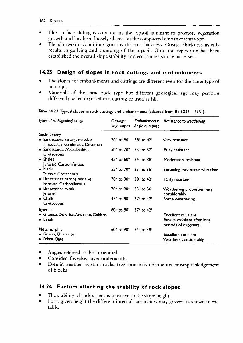
182 Slopes
• This surface sliding is common as the topsoil is meant to promote vegetationgrowth and has been loosely placed on the compacted embankment/slope.
• The short-term conditions governs the soil thickness. Greater thickness usuallyresults in gullying and slumping of the topsoil. Once the vegetation has been established the overall slope stability and erosion resistance increases.
14.23 Design of slopes in rock cuttings and em b ankm en ts• The slopes for embankments and cuttings are different even for the same type of
material.• Materials of the same rock type but different geological age may perform
differently when exposed in a cutting or used as fill.
Table 14.23 Typical slopes in rock cuttings and embankments (adapted from BS 6031 - 1981).
Types o f rock/geological age Cuttings: Safe slopes
Embankments: Angle o f repose
Resistance to weathering
Sedimentary• Sandstones: strong, massive
Triassic; Carboniferous; Devonian70" to 90° 38° to 42° Very resistant
• Sandstones;Weak, bedded Cretaceous
50° to 70° 33 to 37° Fairy resistant
• Shales Jurassic; Carboniferous
45° to 60° 3 4 °to 38 Moderately resistant
• Marls Triassic; Cretaceous
55 to 70° 33° to 36° Softening may occur with time
• Limestones; strong massive Permian; Carboniferous
70° to 90° 38° to 42° Fairly resistant
• Limestones; weak Jurassic
70° to 90° 33° to 36° Weathering properties vary considerably
• Chalk Cretaceous
45° to 80 37° to 42° Some weathering
Igneous• Granite, Dolerite, Andesite, Gabbro• Basalt
80° to 90 37° to 42°Excellent resistant.Basalts exfoliate after long periods of exposure
Metamorphic• Gneiss, Quartzite,• Schist, Slate
60° to 90° 34° to 38°Excellent resistant Weathers considerably
• Angles referred to the horizontal.• Consider if weaker layer underneath.• Even in weather resistant rocks, tree roots may open joints causing dislodgement
of blocks.
14.24 Factors affecting the stabil ity of rock slopes• The stability of rock slopes is sensitive to the slope height.• For a given height the different internal parameters may govern as shown in the
table.
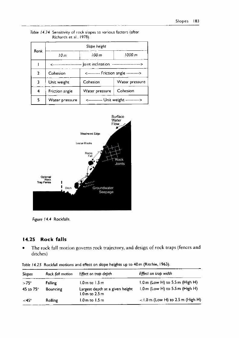
Slopes 183
Table 14.24 Sensitivity of rock slopes to various factors (after Richards et al., 1978).
RankSlope height
10 m 100m 1000 m
1 <.......................... - Joint inclination -..............................>
2 Cohesion <.............Friction angle...............>
3 Unit weight Cohesion W ater pressure
4 Friction angle W ater pressure Cohesion
5 W ater pressure <.............. Unit w eight................>
Optional Rock
Trap Fence
Surface Water > Flow
Weathered Edge
Loose Blocks
Figure 14.4 Rockfalls.
14.25 Rock falls• The rock fall motion governs rock trajectory, and design of rock traps (fences and
ditches)
Table 14.25 Rockfall motions and effect on slope heights up to 40 m (Ritchie, 1963).
Slopes Rock fall motion Effect on trap depth Effect on trap width
>75° Falling 1.0 m to 1.5 m 1.0 m (Low H) to 5.5 m (High H)45 to 75° Bouncing Largest depth at a given height
1.0 m to 2.5 m1.0 m (Low H) to 5.5 m (High H)
<45° Rolling 1.0 m to 1.5 m < 1.0 m (Low H) to 2.5 m (High H)
184 Slopes
• Computing the rock fall motion and remedial measures allows greater flexibilities, in terms of rock sizes, probabilities, varying slope changes, benching, etc. The coefficient of restitution is required in such analysis.
14.26 Coeffic ient of restitution• There are some inconsistencies in various quoted values in referenced paper from
various sources.
Table 14.26 Coefficient of restitution (Richards, 1991).
Type o f material on slope surface Coefficient o f restitution
r Normal rn Tangential rt
Impact between competent materials (Rock-rock) 0.75-0.80Impact between competent rock and soil scree
material0.20-0.35
Solid rock 0.9-0.8 0.75-0.65Detrital material mixed with large rock boulders 0.8-0.5 0.65-0.45Compact detrital material mixed with small boulders 0.5-0.4 0.45-0.35Grass covered slopes or meadows 0.4-0.2 0.3-0.2
14.27 Rock cut stabil ization m easures• Rock slopes that are considered unstable need stabilization or protective measures
needs to be considered.
Table 14.27 Rock slope stabilization considerations.
Consideration Solution Methods Comment
EliminateProblem
Rock Removal • Relocate structure/service/road/rail• Resloping• Trimming and scaling
Relocation is often not possible. Resloping requires additional land
Stabilization Reinforcement • Drainage• Berms• Rock Bolting and Dowels• Tied Back walls• Shotcrete facings
Often expensive solutions
Reduce Hazard ProtectionMeasures
• Mesh over slope• Rock Trap ditches• Fences• Berms• Barriers and impact walls• False Tunnels
Controls the rock falls. Usually cheapest solution. Requires some maintenance e.g. clearing rock behind mesh
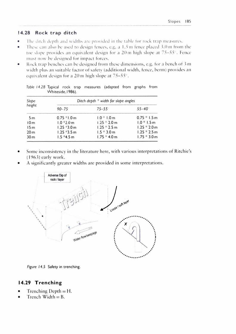
Slopes 185
I 4.28 R o c k t r a p d itch• I he ditch depth and widths are provided in the table for rock trap measures.• T h e s e can also be used to design fences, e.g. a 1.5 m fence placed 3.0 m from the
toe slope provides an equivalent design tor a 20 m high slope at 7 5 - 5 5 . Fence must now be designed for impact forces.
• Rock trap benches can be designed from these dimensions, e.g. for a bench of 3 m width plus an suitable factor of safety (additional width, fence, berm) provides an equivalent design for a 20 m high slope at 7 5 - 5 5 ° .
Table 14.28 Typical rock trap measures (adapted from graphs from Whiteside, 1986).
Slopeheight
Ditch depth * width for slope angles
90-75 75-55 55-4 0
5 m 0.75 *1.0 m 1.0 * 1.0 m 0.75 * 1.5 m10 m 1.0 *2.0 m i .25 * 2.0 m 1.0* 1.5 m15 m 1.25 *3.0 m 1.25 * 2.5 m 1.25 * 2.0 m20 m 1.25 *3.5 m 1.5 * 3.0 m 1.25 * 2.5 m30 m 1.5 *4.5 m 1.75 * 4.0 m 1.75 * 3.0 m
Some inconsistency in the literature here, with various interpretations of Ritchie’s (1963) early work.A significantly greater widths are provided in some interpretations.
Adverse Dip of rock I layer
% c
Figure 14.5 Safety in trenching.
14.29 Trench ing• Trenching Depth = FI.• Trench Width = B.
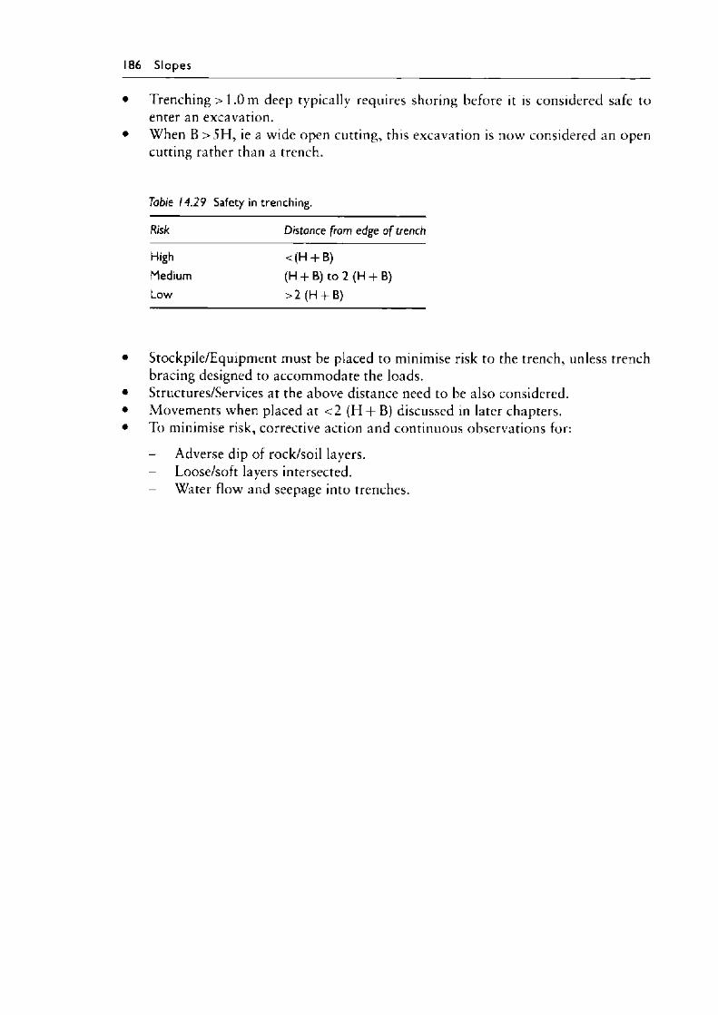
186 Slopes
• Trenching > 1.0 m deep typically requires shoring before it is considered safe to enter an excavation.
• When B > 5 H , ie a wide open cutting, this excavation is now considered an open cutting rather than a trench.
Table 14.29 Safety in trenching.
Risk Distance from edge o f trench
High <(H + B)Medium (H + B) to 2 (H + B)Low >2 (H + B)
• Stockpile/Equipment must be placed to minimise risk to the trench, unless trench bracing designed to accommodate the loads.
• Structures/Services at the above distance need to be also considered.• Movements when placed at < 2 (H + B) discussed in later chapters.• To minimise risk, corrective action and continuous observations for:
- Adverse dip of rock/soil layers.- Loose/soft layers intersected.
Water flow and seepage into trenches.
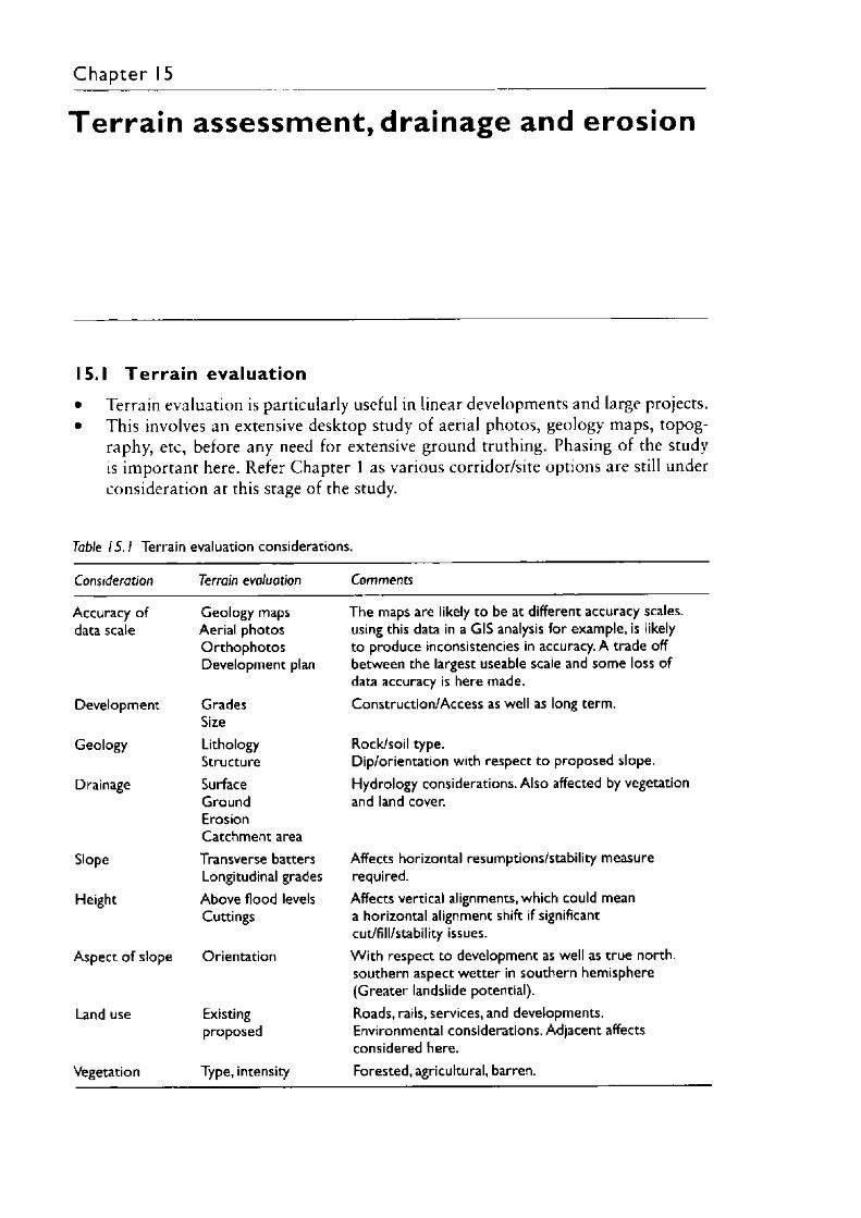
Chapter 15
T e rra in assessm ent, drainage and erosion
15.1 T e r ra in evaluation• Terrain evaluation is particularly useful in linear developments and large projects.• This involves an extensive desktop study of aerial photos, geology maps, topog
raphy, etc, before any need for extensive ground truthing. Phasing of rhe study is important here. Refer Chapter 1 as various corridor/site options are still under consideration at this stage of the study.
Table 15.1 Terrain evaluation considerations.
Consideration Terrain evaluation Comments
Accuracy of Geology maps The maps are likely to be at different accuracy scales.data scale Aerial photos
Orthophotos Development plan
using this data in a GIS analysis for example, is likely to produce inconsistencies in accuracy. A trade off between the largest useable scale and some loss of data accuracy is here made.
Development GradesSize
Construction/Access as well as long term.
Geology LithologyStructure
Rock/soil type.Dip/orientation with respect to proposed slope.
Drainage SurfaceGroundErosionCatchment area
Hydrology considerations. Also affected by vegetation and land cover.
Slope Transverse batters Longitudinal grades
Affects horizontal resumptions/stability measure required.
Height Above flood levels Cuttings
Affects vertical alignments, which could mean a horizontal alignment shift if significant cut/fill/stability issues.
Aspect of slope Orientation W ith respect to development as well as true north, southern aspect wetter in southern hemisphere (Greater landslide potential).
Land use Existingproposed
Roads, rails, services, and developments. Environmental considerations. Adjacent affects considered here.
Vegetation Type, intensity Forested, agricultural, barren.
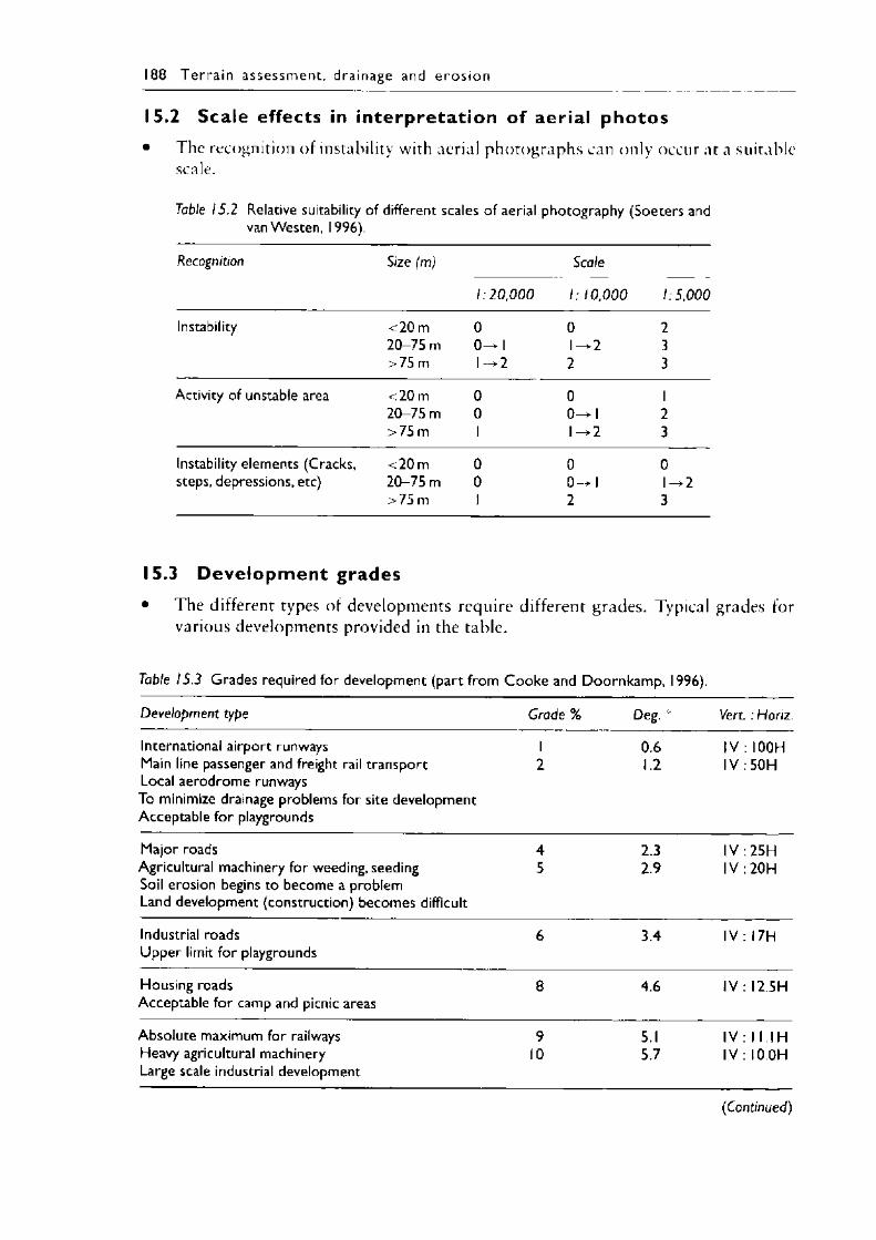
188 T e r ra in a ssessm ent , drainage and e ro s io n
15.2 Scale effects in in terpretat ion of aer ia l photos• The recognition of instability with aerial photographs can only occur at a suitable
scale.
Table 15.2 Relative suitability of different scales of aerial photography (Soeters and vanWesten, 1996).
Recognition Size (m)
1 :20 ,000
Scale
1: 10,000 1 :5,000
Instability <20 m 0 0 220-75 m 0-> 1 1 —>2 3>75 m l-> 2 2 3
Activity of unstable area <20 m 0 0 12 0 -7 5 m 0 0 ^ 1 2>75 m 1 1 - * 2 3
Instability elements (Cracks, <20 m 0 0 0steps, depressions, etc) 20-75 m 0 0-> l 1 —>2
>75 m 1 2 3
15.3 Development grades• The different types of developments require different grades. Typical grades for
various developments provided in the table.
Table 15.3 Grades required for development (part from Cooke and Doornkamp, 1996).
Development type Grade % Deg. 0 Vert. : Horiz.
International airport runwaysMain line passenger and freight rail transportLocal aerodrome runwaysTo minimize drainage problems for site development Acceptable for playgrounds
12
0.61.2
IV : I00H IV :50H
Major roads 4 2.3 IV :25HAgricultural machinery for weeding, seedingSoil erosion begins to become a problemLand development (construction) becomes difficult
5 2.9 IV :20H
Industrial roadsUpper limit for playgrounds
6 3.4 IV : I7H
Housing roadsAcceptable for camp and picnic areas
8 4.6 IV : I2.5H
Absolute maximum for railways 9 5.1 IV : 1 I .IHHeavy agricultural machinery Large scale industrial development
10 5.7 IV : I0.0H
(Continued)
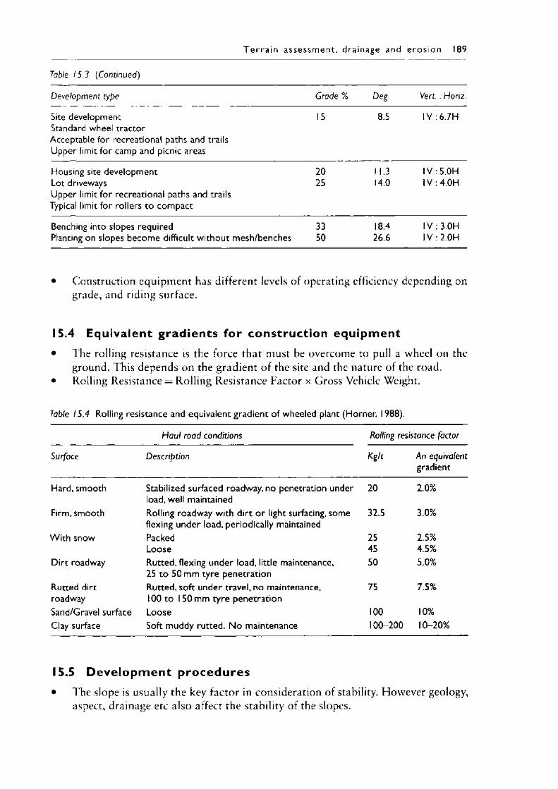
T e r r a in asse ssm en t , drainage and e ro s io n 189
Table 15.3 (Continued)
Development type Grade % Deg. 5 X o N
Site developmentStandard wheel tractorAcceptable for recreational paths and trailsUpper limit for camp and picnic areas
15 8.5 IV :6.7H
Housing site development 20 1 1.3 IV :5.0HLot drivewaysUpper limit for recreational paths and trails Typical limit for rollers to compact
25 14.0 1V : 4.OH
Benching into slopes required 33 18.4 IV : 3.OHPlanting on slopes become difficult without mesh/benches 50 26.6 IV : 2.OH
• Construction equipment has different levels of operating efficiency depending ongrade, and riding surface.
15.4 Equ ivalent gradients for construct ion equipment• The rolling resistance is the force that must he overcome to pull a wheel on the
ground. This depends on the gradient of the site and the nature of the road.• Rolling Resistance = Rolling Resistance Factor x Gross Vehicle Weight.
Table 15.4 Rolling resistance and equivalent gradient of wheeled plant (Horner, 1988).
Haul road conditions Rolling resistance factor
Surface Description Kg/t An equivalentgradient
Hard, smooth Stabilized surfaced roadway, no penetration under load, well maintained
20 2.0%
Firm, smooth Rolling roadway with dirt or light surfacing, some flexing under load, periodically maintained
32.5 3.0%
W ith snow Packed 25 2.5%Loose 45 4.5%
Dirt roadway Rutted, flexing under load, little maintenance, 25 to 50 mm tyre penetration
50 5.0%
Rutted dirt Rutted, soft under travel, no maintenance, 75 7.5%roadway 100 to 150 mm tyre penetrationSand/Gravel surface Loose 100 10%Clay surface Soft muddy rutted. No maintenance 100-200 10-20%
15.5 D eve lo p m ent p ro cedu res• The slope is usually the key factor in consideration of stability. Flowever geology,
aspect, drainage etc also affect the stability of the slopes.
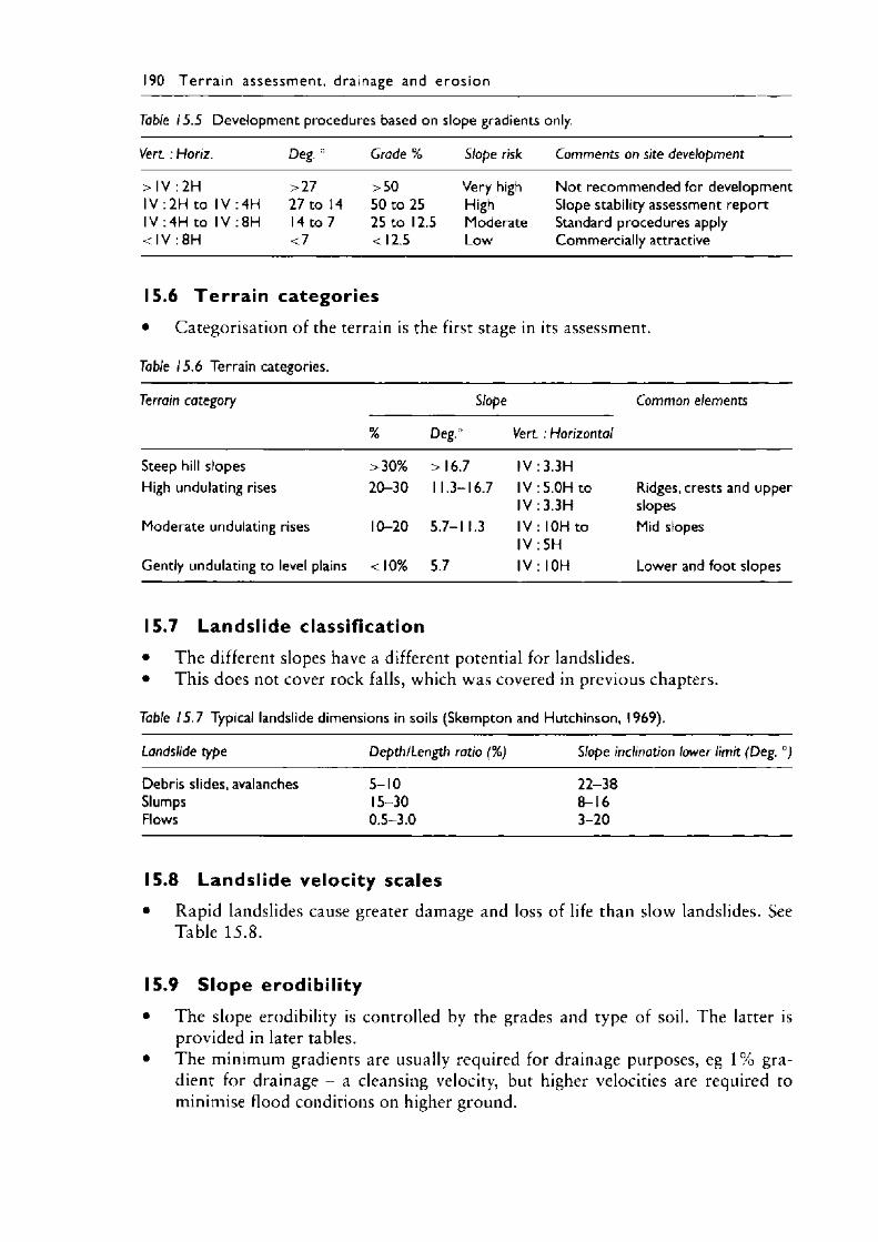
190 T e r r a in assessm ent , drainage and e ro s io n
Table 15.5 Development procedures based on slope gradients only.
Vert. : Horiz. Deg. ° Grade % Slope risk Comments on site development
IrN>A >27 >50 Very high Not recommended for developmentIV :2H to IV :4H 27 to 14 50 to 25 High Slope stability assessment reportIV :4H to IV :8H 14 to 7 25 to 12.5 Moderate Standard procedures applyI00>V <7 <12.5 Low Commercially attractive
15.6 T e r ra in categories• Categorisation of the terrain is the first stage in its assessment.
Table 15.6 Terrain categories.
Terrain category
%
Slope
Deg.° Vert : Horizontal
Common elements
Steep hill slopes >30% >16.7 IV :3.3HHigh undulating rises 20-30 1 1.3-16.7 IV :5.0H to Ridges, crests and upper
IV : 3.3H slopesModerate undulating rises 10-20 5.7-1 1.3 IV : I0H to Mid slopes
IV :5HGently undulating to level plains <10% 5.7 IV : I0H Lower and foot slopes
15.7 Landslide classification• The different slopes have a different potential for landslides.• This does not cover rock falls, which was covered in previous chapters.
Table 15.7 Typical landslide dimensions in soils (Skempton and Hutchinson, 1969).
Landslide type Depth/Length ratio (%) Slope inclination lower limit (Deg. °)
Debris slides, avalanches 5-10 22-38Slumps 15-30 8-16Flows 0.5-3.0 3-20
15.8 Landslide velocity scales• Rapid landslides cause greater damage and loss of life than slow landslides. See
Table 15.8.
15.9 Slope erodibil ity• The slope erodibility is controlled by the grades and type of soil. The latter is
provided in later tables.• The minimum gradients are usually required for drainage purposes, eg 1% gra
dient for drainage - a cleansing velocity, but higher velocities are required to minimise flood conditions on higher ground.
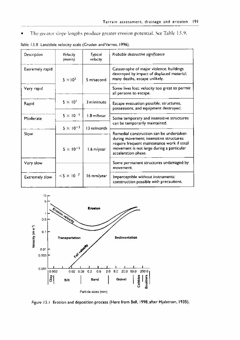
T e r ra in asse ssm en t , drainage and e ro s io n 191
• The greater slope lengths produce greater erosion potential. See Table 15.9.
Table 15.8 Landslide velocity scale (Cruden andVarnes, 1996).
Description Velocity(mm/s)
Typicalvelocity
Probable destructive significance
Extremely rapid
5 x I0 3 5 m/second
Catastrophe of major violence; buildings destroyed by impact of displaced material; many deaths, escape unlikely.
Very rapid Some lives lost; velocity too great to permit all persons to escape.
5 x 10' 3 m/minuteRapid Escape evacuation possible; structures, possessions, and equipment destroyed.
5 x 10 1 1.8 m/hourModerate Some temporary and insensitive structures can be temporarily maintained.
5 x 10 3 13 m/monthSlow Remedial construction can be undertaken
during movement; insensitive structures require frequent maintenance work if total movement is not large during a particular acceleration phase.
5 x 10 5 1.6 m/year
Very slow Some permanent structures undamaged by movement.
< 5 X 1 0 7 16 mm/yearExtremely slow Imperceptible without instruments; construction possible with precautions.
Figure 15.1 Erosion and deposition process (Here from Bell, 1998, after Hjulstrom, 1935).
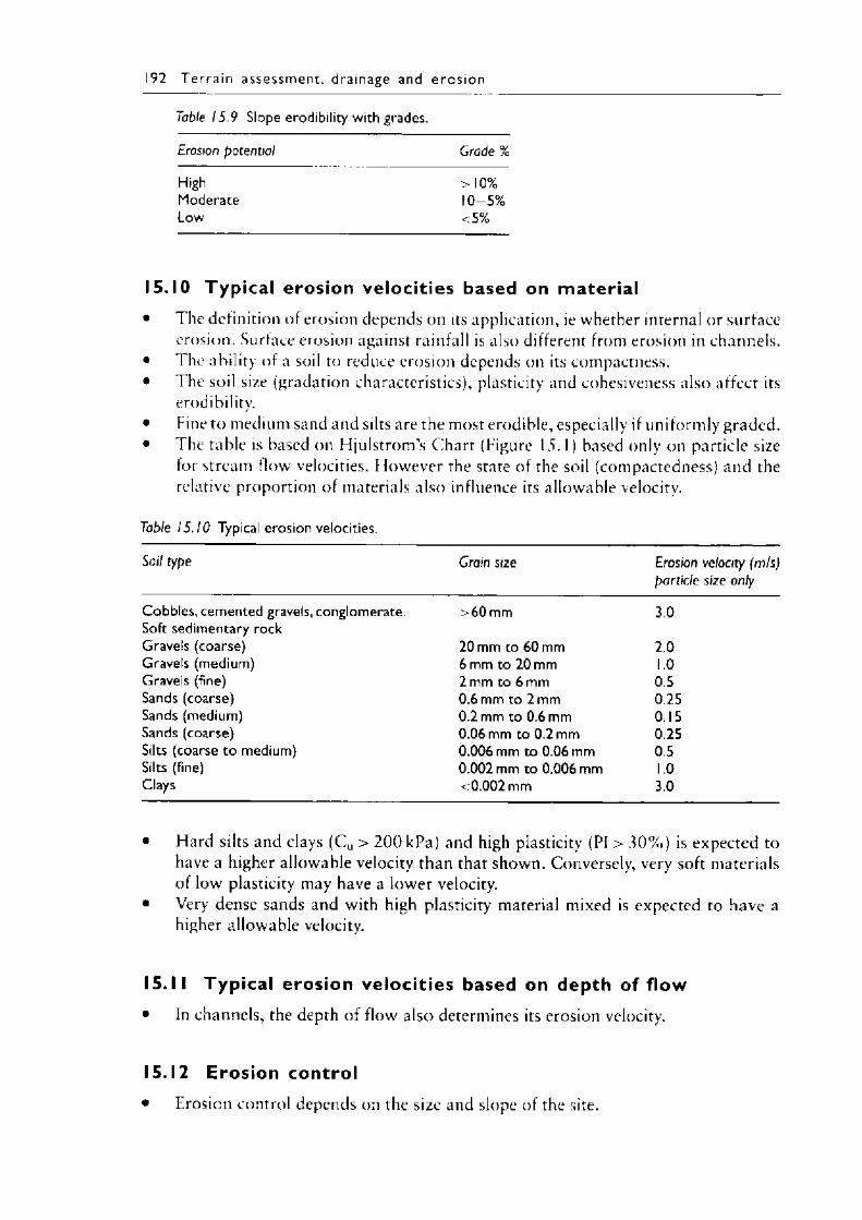
192 T e r r a in a ssessm ent , drainage and e ro s io n
Table 15.9 Slope erodibility with grades.
Erosion potential Grade %
High > 10%Moderate 10-5%Low <5%
15.10 Typical erosion velocities based on material• 1 he definition of erosion depends on its application, ie whether internal or surface
erosion. Surface erosion against rainfall is also different from erosion in channels.• The ability of a soil to reduce erosion depends on its compactness.• The soil size (gradation characteristics), plasticity and cohesiveness also affect its
erodibility.• Fine to medium sand and silts are the most erodible, especially if uniformly graded.• The table is based on Hjulstrom s Chart (Figure 15.1) based only on particle size
for stream flow velocities. However the state of the soil (compactedness) and the relative proportion of materials also influence its allowable velocity.
Table 15.10 Typical erosion velocities.
Soil type Grain size Erosion velocity (m/s) particle size only
Cobbles, cemented gravels, conglomerate. >60 mm 3.0Soft sedimentary rockGravels (coarse) 20 mm to 60 mm 2.0Gravels (medium) 6 mm to 20 mm 1.0Gravels (fine) 2 mm to 6 mm 0.5Sands (coarse) 0.6 mm to 2 mm 0.25Sands (medium) 0.2 mm to 0.6 mm 0.15Sands (coarse) 0.06 mm to 0.2 mm 0.25Silts (coarse to medium) 0.006 mm to 0.06 mm 0.5Silts (fine) 0.002 mm to 0.006 mm 1.0Clays <0.002 mm 3.0
• Hard silts and clays (Cu > 2 0 0 kPa) and high plasticity (PI > 3 0 % ) is expected to have a higher allowable velocity than that shown. Conversely, very soft materials of low plasticity may have a lower velocity.
• Very dense sands and with high plasticity material mixed is expected to have a higher allowable velocity.
15.11 Typical erosion velocit ies based on depth of flow• In channels, the depth of flow also determines its erosion velocity.
15.12 Erosion control• Erosion control depends on the size and slope of the site.
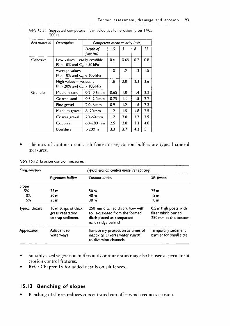
T e r ra in a ssessm ent , drainage and e ro s io n 193
Table 15 .11 Suggested competent mean velocities for erosion (after TAC, 2004).
Bed material Description Competent mean velocity (m/s)Depth o f flow (m)
1.5 3 6 15
Cohesive Low values - easily erodible Pl< 10% and C u < 50 kPa
0.6 0.65 0.7 0.8
Average valuesPl> 10% and C u < lOOkPa
1.0 1.2 1.3 1.5
High values - resistant PI >20% and C u > lOOkPa
1.8 2.0 2.3 2.6
Granular Medium sand 0.2-0.6 mm 0.65 1.0 1.4 2.2Coarse sand 0.6-2.0 mm 0.75 l.l 1.5 2.2Fine gravel 2.0-6 mm 0.9 1.2 1.6 2.3Medium gravel 6-20 mm 1.2 1.5 1.8 2.5Coarse gravel 20-60 mm 1.7 2.0 2.2 2.9Cobbles 60-200 mm 2.5 2.8 3.3 4.0Boulders >200 m 3.3 3.7 4.2 5
• The uses of contour drains, silt fences or vegetation buffers arc typical control measures.
Table 15.12 Erosion control measures.
Consideration Typical erosion control measures spacing
Vegetation buffers Contour drains Silt fences
Slope5% 75 m 50 m 25 m10% 50 m 40 m 15 m15% 25 m 30 m 10 m
Typical details 10 m strips of thick grass vegetation to trap sediment
250 mm ditch to divert flow with soil excavated from the formed ditch placed as compacted earth ridge behind
0.5 m high posts with filter fabric buried 250 mm at the bottom
Application Adjacent to waterways
Temporary protection at times of inactivity. Diverts water runoff to diversion channels
Temporary sediment barrier for small sites
• Suitably sized vegetation buffers and contour drains may also be used as permanent erosion control features.
• Refer Chapter 16 for added details on silt fences.
15.13 Benching of slopes• Benching of slopes reduces concentrated run off - which reduces erosion.
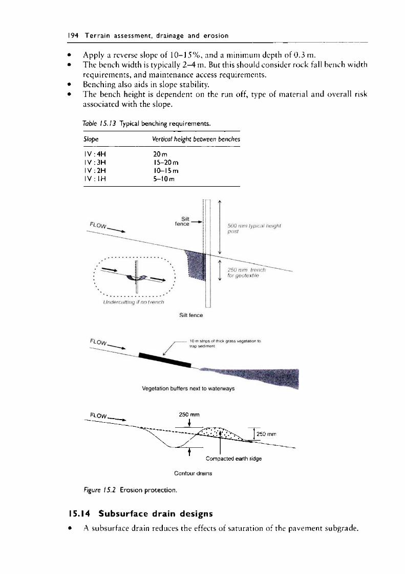
194 T e r r a in a s sessm ent , drainage and e ro s io n
• Apply a reverse slope of 1 0 - 1 5 % , and a minimum depth of 0 .3 m.• The bench width is typically 2 - 4 m. But this should consider rock fall bench width
requirements, and maintenance access requirements.• Benching also aids in slope stability.• The bench height is dependent on the run off, type of material and overall risk
associated with the slope.
Table 15.13 Typical benching requirements.
Slope Vertical height between benches
IV :4H 20 m1V : 3H 15-20 mIV :2H 10-15 mIV : IH 5-10 m
Contour drains
Figure 15.2 Erosion protection.
15.14 Subsurface drain designs• A subsurface drain reduces the effects of saturation of the pavement subgrade.
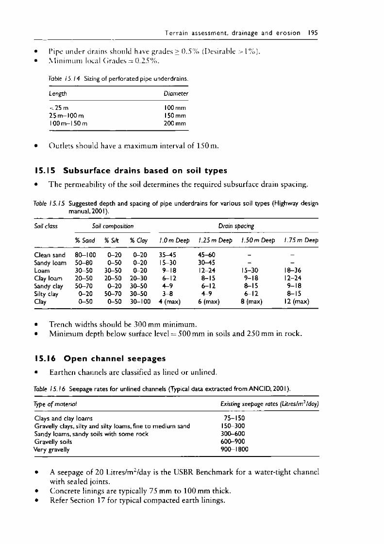
T e r ra in a s sessm ent , drainage and e ro s io n 195
Pipe under drains should have grades > 0 . 5 % (Desirable > 1% Minimum local Grades = 0 .2 5 % .
Table 15 .14 Sizing of perforated pipe underdrains.
Length Diameter
<25 m 100 mm25 m-100 m 150 mm1 00 m - 1 50 m 200 mm
• Outlets should have a maximum interval of 150 m.
15.15 Subsurface drains based on soil types• The permeability of the soil determines the required subsurface drain spacing.
Table 15.15 Suggested depth and spacing of pipe underdrains for various soil types (Highway design manual, 2001).
Soil class Soil composition Drain spacing
% Sand % Silt % Clay 1.0 m Deep 1.25 m Deep 1.50 m Deep 1.75 m Deef.
Clean sand 80-100 0-20 0-20 35—45 45-60 — —
Sandy loam 50-80 0-50 0-20 15-30 30-45 - -
Loam 30-50 30-50 0-20 9-18 12-24 15-30 18-36Clay loam 20-50 20-50 20-30 6-12 8-15 9-18 12-24Sandy clay 50-70 0-20 30-50 4-9 6-12 8-15 9-18Silty clay 0-20 50-70 30-50 3-8 4-9 6-12 8-15Clay 0-50 0-50 30-100 4 (max) 6 (max) 8 (max) 12 (max)
• Trench widths should be 300 mm minimum.• Minimum depth below surface level = 5 0 0 mm in soils and 2 5 0 mm in rock.
15.16 O p en channel seepages• Earthen channels are classified as lined or unlined.
Table 15.16 Seepage rates for unlined channels (Typical data extracted from A N CID , 2001).
Type o f material Existing seepage rates (Litres/m2/day)
Clays and clay loamsGravelly clays, silty and silty loams, fine to medium sand Sandy loams, sandy soils with some rock Gravelly soils Very gravelly
75-150 150-300 300-600 600-900 900-1800
• A seepage of 2 0 Litres/m2/day is the USBR Benchmark for a water-tight channel with sealed joints.
• Concrete linings are typically 75 mm to 100 mm thick.• Refer Section 17 for typical compacted earth linings.
196 T e r r a in a s sessm ent , dra inage and e ro s io n
• Compacted Clay linings at the bottom of a channel typically 0 .5 m thick can reduce the seepage by 8 0 % to 5 0 % for very gravelly soils to fine sand materials, respectively.
• Geosynthetic Clay Liners (GCLs) and Geomembranes can also be used with 2 5 0 mm minimum soil cover.
Width of canal, B .
A ssess
Figure 15.3 Canal issues to be assessed during investigation.
15.17 C om par ison between open channel flows and seepages through soils
• Hydraulic Gradient of 0.01 in all cases.
Table 15.17 Comparisons between flows in open channels and pipes and seepage through soils and aggregates, Cedergren ( 1989).
Flow medium Effective channel diameter
Flow (m3/s) Area (m 2) for discharge o f 50 mm pipe
Smooth channel 24 m = 2R 12,000Smooth pipe 2.4m = d 20
0.30 m = d 0.150 mm = d 4 x 10 4 5 0 mm pipe (0 .2m2)
25 mm to 40 mm gravel 5 mm # 4 x 10 4 0.112 mm to 25 mm gravel 2.5 mm # 1 x 10 4 0.35 mm to 10 mm gravel 0.75 mm # 2 x 10 5 2.0Coarse sand 0.25 mm # 3 x 10 6 17Fine sand, or graded filter aggregate 0.05 mm # 3 x 10 8 1.7 x I0 3Silt 0.006 mm # 3 x 10 11 1.7 x I06Fat clay 0.001 mm # 3 x 10 13 1.8 x I08
• # Per 0 .93 x 10 square metre area.
Borehole/test to appropriate depth
T e r r a in a ssessm ent , drainage and e ro s io n 197
15.18 Drainage measures factors of safety• l arge factors of safety are applied in drainage situations due to the greater
uncertainties with ground water associated issues.
Table 15.18 Factors of safety for drainage measures.
Drainage element Factor o f safety
Comments
Pipes 2 To avoid internal piezometric pressures.Granular material 10 To avoid permeability reduction due to fines or turbulent
flows.Geotextiles 10 To account for distortion and clogging.Blanket drain on flat slope 10 To avoid permeability reduction due to fines or turbulent
flows.Blanket drain on steep slope 5 eg chimney drains, which uses graded filter or geotextile.Geocomposite 4 To account for crushing.
15.19 Aggregate drains• Aggregate drains are often used for internal drainage of the soil.
Table 15.19 Aggregate drains.
Aggregate type Advantages Disadvantages
Open graded gravels - french drain Good flow capacity Clogging by piping from surrounding soils
Well graded sands - filter sands Resists piping. Useful in reduction in pore water pressures
Low flow capacity
Open graded gravels wrapped in Resists piping. Reasonable flow Depth limitationgeotextile capacity
15.20 Aggregate drainage• Aggregate drains are sometimes used with or in place of agricultural perforated
pipes. The pipes channel the already collected water while the aggregate drains the surrounding soils.
• The equivalent permeability for various size aggregate is provided in the table.• There is a significant advantage of using large size aggregate in terms of increased
permeability (flows) and reduced size.• No factors of safety apply.• 1 = 1 % to minimise turbulent effects in the aggregate.
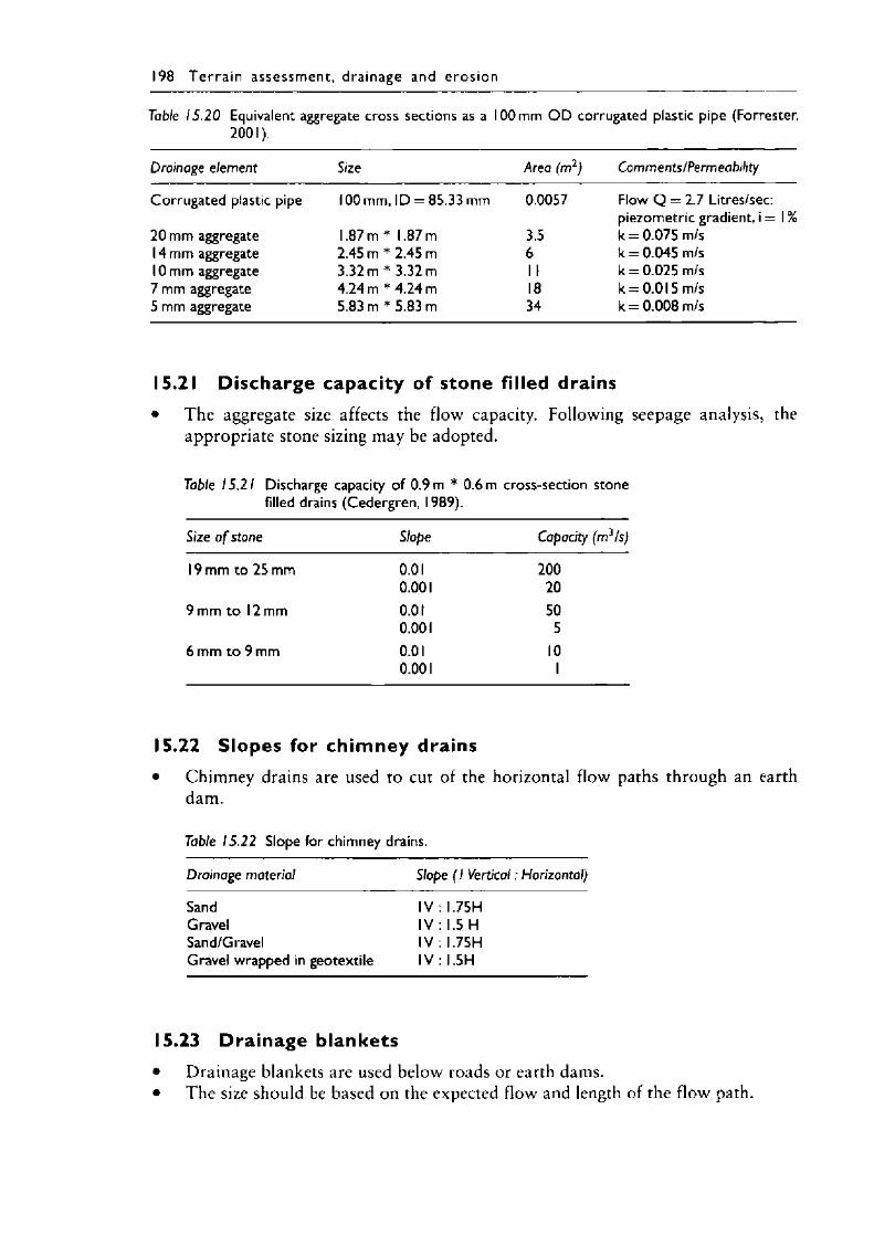
198 T e r r a in asse ssm en t , dra inage and e ro s io n
Table 15.20 Equivalent aggregate cross sections as a 100 mm O D corrugated plastic pipe (Forrester, 2001 ).
Drainage element Size Area (m2) Comments/Permeability
Corrugated plastic pipe 100 mm, ID = 85.33 mm 0.0057 Flow Q = 2.7 Litres/sec:piezometric gradient, i = 1%
20 mm aggregate 1.87m * 1.87m 3.5 k = 0.075 m/s14 mm aggregate 2.45 m * 2.45 m 6 k = 0.045 m/s10 mm aggregate 3.32 m * 3.32 m 1 1 k = 0.025 m/s7 mm aggregate 4.24 m * 4.24 m 18 k = 0.015 m/s5 mm aggregate 5.83 m * 5.83 m 34 k = 0.008 m/s
15.21 Discharge capacity of stone filled drains• The aggregate size affects the flow capacity. Following seepage analysis, the
appropriate stone sizing may be adopted.
Table 15.21 Discharge capacity of 0.9 m * 0.6 m cross-section stone filled drains (Cedergren, 1989).
Size o f stone Slope Capacity (m3/s)
19 mm to 25 mm 0.01 2000.001 20
9 mm to 12 mm 0.01 500.001 5
6 mm to 9 mm 0.01 100.001 1
15.22 Slopes for ch im ney drains• Chimney drains are used to cut of the horizontal flow paths through an earth
dam.
Table 15.22 Slope for chimney drains.
Drainage material Slope (1 Vertical: Horizontal)
Sand IV I.75HGravel IV 1.5 HSand/Gravel IV I.75HGravel wrapped in geotextile IV I.5H
15.23 Drainage blankets• Drainage blankets are used below roads or earth dams.• The size should be based on the expected flow and length of the flow path.
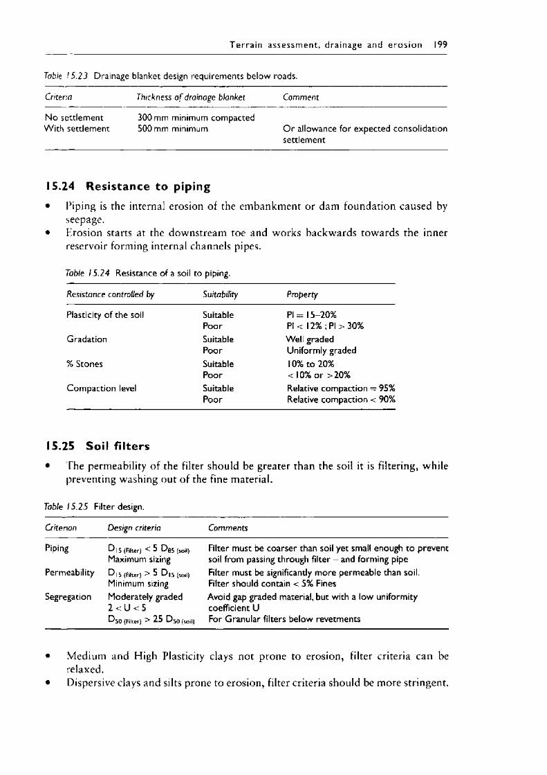
T e r ra in a ssessm ent , drainage and e ro s io n 199
Table 15.23 Drainage blanket design requirements below roads.
Criteria Thickness o f drainage blanket Comment
No settlement 300 mm minimum compactedWith settlement 500 mm minimum O r allowance for expected consolidation
settlement
15.24 Resistance to piping• Piping is the internal erosion of the embankment or dam foundation caused by
seepage.• Erosion starts at the downstream toe and works backwards towards the inner
reservoir forming internal channels pipes.
Table 15.24 Resistance of a soil to piping.
Resistance controlled by Suitability Property
Plasticity of the soil Suitable P l= 15-20%Poor P l< 12%; PI >30%
Gradation Suitable Well gradedPoor Uniformly graded
% Stones Suitable 10% to 20%Poor <10% or >20%
Compaction level Suitable Relative compaction = 95%Poor Relative compaction < 90%
15.25 Soil filters• The permeability of the filter should be greater than the soil it is filtering, while
preventing washing out of the fine material.
Table 15.25 Filter design.
Criterion Design criteria Comments
Piping D 15 (Filter) < 5 Das (soil)
Maximum sizingFilter must be coarser than soil yet small enough to prevent soil from passing through filter - and forming pipe
Permeability D 15 (Filter) > 5 D 15 (soi|)
Minimum sizingFilter must be significantly more permeable than soil. Filter should contain < 5% Fines
Segregation Moderately graded 2 < U < 5
Avoid gap graded material, but with a low uniformity coefficient U
D50 (Filter) > 25 D50 (soil) For Granular filters below revetments
• Medium and High Plasticity clays not prone to erosion, filter criteria can be relaxed.
• Dispersive clays and silts prone to erosion, filter criteria should be more stringent.
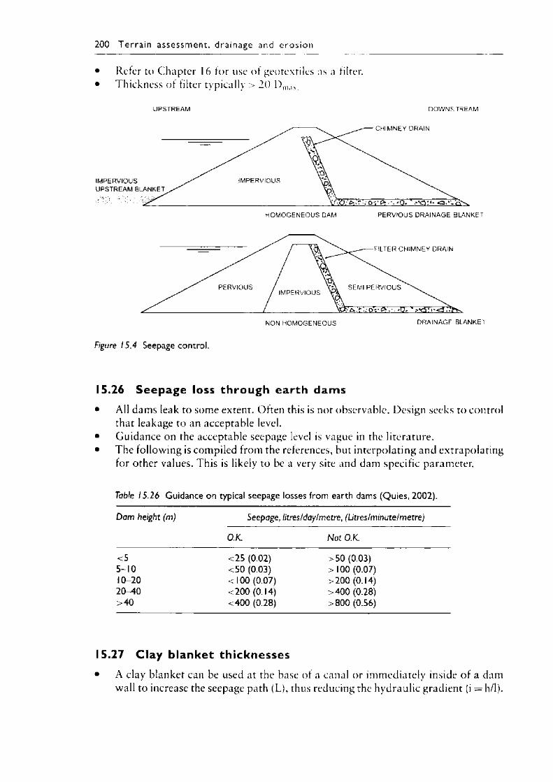
200 T e r r a in a ssessm ent , dra inage and e ro s io n
• Refer to Chapter 16 for use of geotextiles as a filter.• Thickness of filter typically > 20 Dm<lv
UPSTREAM DOWNS.TREAM
Figure 15.4 Seepage control.
15.26 Seepage loss through earth dams• All dams leak to some extent. Often this is not observable. Design seeks to control
that leakage to an acceptable level.• Guidance on the acceptable seepage level is vague in the literature.• The following is compiled from the references, but interpolating and extrapolating
for other values. This is likely to be a very site and dam specific parameter.
Table 15.26 Guidance on typical seepage losses from earth dams (Quies, 2002).
Dam height (m) Seepage, litres/day/metre, (Litres/minute/metre)
O.K. Not O.K.
<5 <25 (0.02) >50 (0.03)5-10 <50 (0.03) >100 (0.07)10-20 <100 (0.07) >200 (0.14)20—40 <200 (0.14) >400 (0.28)>40 <400 (0.28) >800 (0.56)
15.27 C lay blanket thicknesses• A clay blanket can be used at the base of a canal or immediately inside of a dam
wall to increase the seepage path (L), thus reducing the hydraulic gradient (i = h/1).
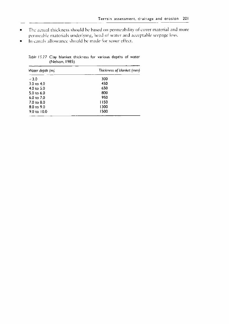
T e r r a in a ssessm ent , drainage and e ro s io n 201
• The actual thickness should he based on permeability of cover material and morepermeable materials underlying, head of water and acceptable seepage loss.
• In canals allowance should be made for scour effect.
Table 15.27 Clay blanket thickness for various depths of water (Nelson, 1985).
Water depth (m) Thickness o f blanket (mm)
<3.0 3003.0 to 4.0 4504.0 to 5.0 6505.0 to 6.0 8006.0 to 7.0 9507.0 to 8.0 1 1508.0 to 9.0 13009.0 to 10.0 1500

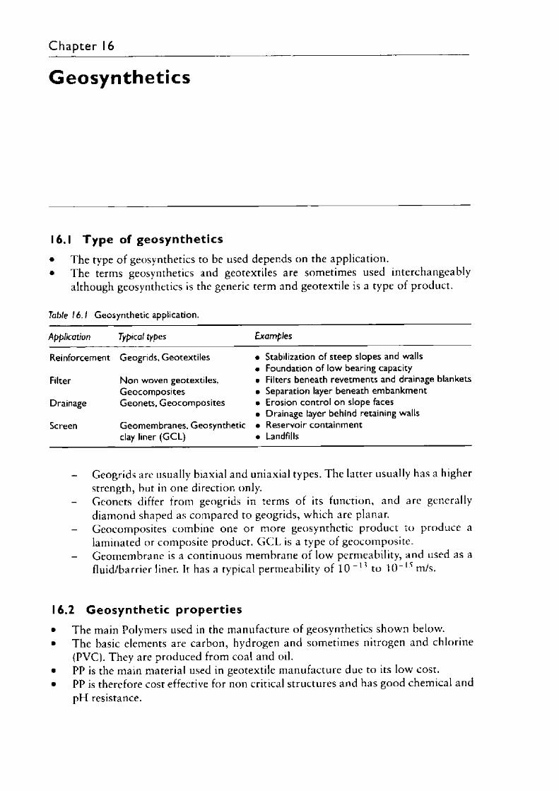
Chapter 16
G eosynthetics
16.1 Type of geosynthetics• The type of geosynthetics to be used depends on the application.• The terms geosynthetics and geotextiles are sometimes used interchangeably
although geosynthetics is the generic term and geotextile is a type of product.
Table 16.1 Geosynthetic application.
Application Typical types Examples
Reinforcement Geogrids, Geotextiles
Filter Non woven geotextiles.Geocomposites
Drainage Geonets, Geocomposites
Screen Geomembranes, Geosyntheticclay liner (G C L)
Stabilization of steep slopes and walls Foundation of low bearing capacity Filters beneath revetments and drainage blankets Separation layer beneath embankment Erosion control on slope faces Drainage layer behind retaining walls Reservoir containment Landfills
Geogrids are usually biaxial and uniaxial types. The latter usually has a higher strength, but in one direction only.Geonets differ from geogrids in terms o f its function, and are generally diamond shaped as compared to geogrids, which are planar.Geocomposites combine one or more geosynthetic product to produce a laminated or composite product. G C L is a type of geocomposite. Geomembrane is a continuous membrane of low permeability, and used as a fluid/barrier liner. It has a typical permeability of 1 0 - n to 10 m/s.
16.2 G eo synthet ic propert ies• The main Polymers used in the manufacture o f geosynthetics shown below.• The basic elements are carbon, hydrogen and sometimes nitrogen and chlorine
(PVC). They are produced from coal and oil.• PP is the main material used in geotextile manufacture due to its low cost.• PP is therefore cost effective for non critical structures and has good chemical and
pH resistance.
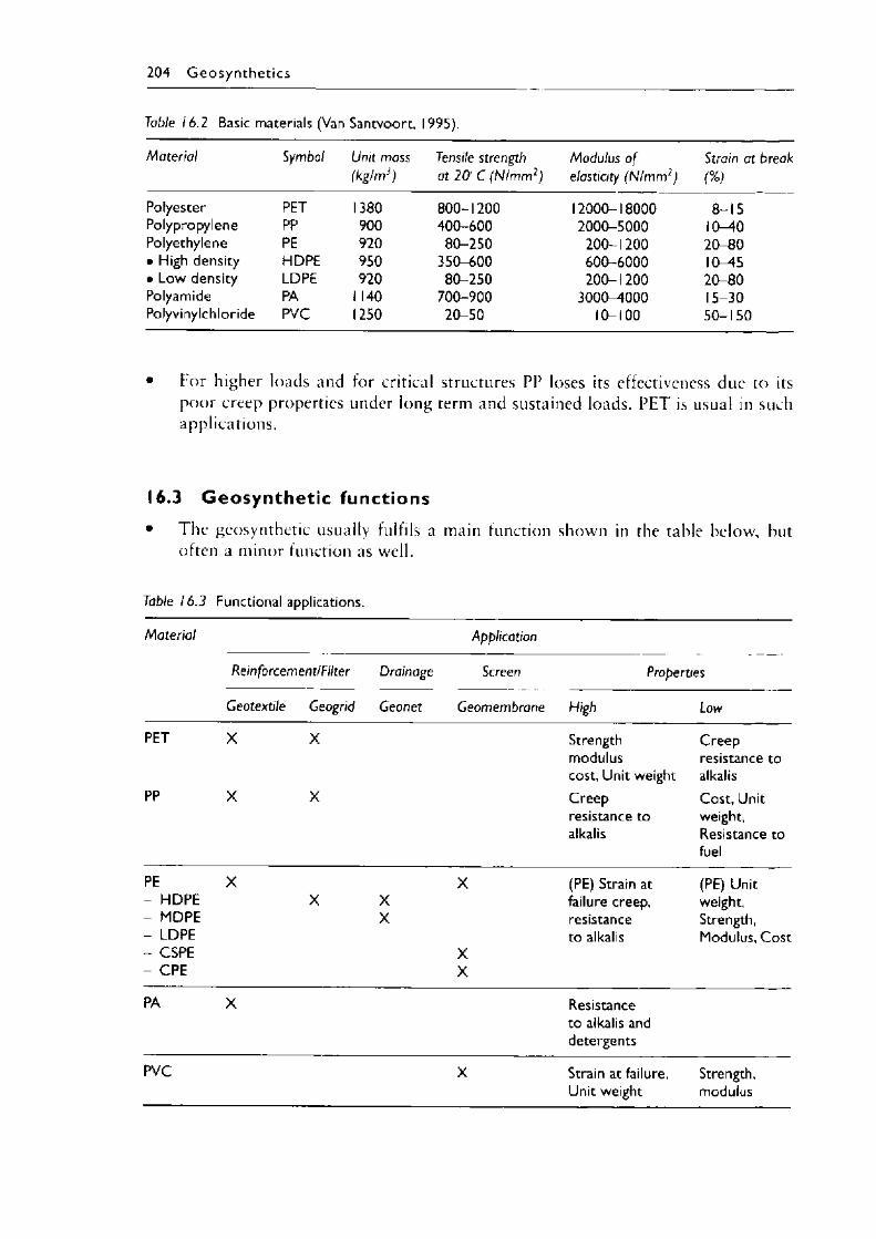
204 G e o s y n th e t ic s
Table 16.2 Basic materials (Van Santvoort, 1995).
Material Symbol Unit mass (kg/m3)
Tensile strength at 20 C (N/mm2)
Modulus o f elasticity (N/mm2)
Strain at break<%)
Polyester PET 1380 800-1200 12000-18000 8-15Polypropylene PP 900 400-600 2000-5000 10-40Polyethylene PE 920 80-250 200-1200 20-80• High density HDPE 950 350-600 600-6000 10—45• Low density LDPE 920 80-250 200-1200 20-80Polyamide PA 1 140 700-900 3000-4000 15-30Polyvinylchloride PVC 1250 20-50 10-100 50-150
For higher loads and for critical structures PP loses its effectiveness due to its poor creep properties under long term and sustained loads. PET is usual in such applications.
16.3 G eosynthet ic functions• The geosynthetic usually fulfils a
often a minor function as well.
Table 16.3 Functional applications.
main function shown in the ta hie he low, but
Material Application
Reinforcement/Filter Drainage Screen Properties
Geotextile Geogrid Geonet Geomembrane High Low
PET X X Strength Creepmodulus resistance tocost, Unit weight alkalis
PP X X Creep Cost, Unitresistance to weight,alkalis Resistance to
fuel
PE X X (PE) Strain at (PE) Unit- HDPE X X failure creep, weight,- MDPE X resistance Strength,- LDPE to alkalis Modulus, Cost- CSPE X- CPE X
PA X Resistanceto alkalis anddetergents
PVC X Strain at failure, Strength,Unit weight modulus
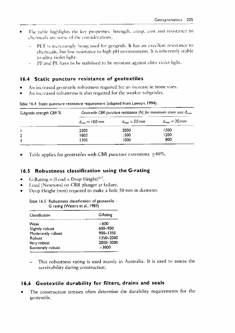
• The table highlights the key properties. Strength, creep, cost and resistance to chemicals are some of the considerations.
- PET is increasingly being used for geogrids. It has an excellent resistance to chemicals, but low resistance to high pH environments. It is inherently stable to ultra violet light.PP and PE have to be stabilised to be resistant against ultra violet light.
16.4 Stat ic puncture resistance of geotextiles• An increased geotextile robustness required for an increase in stone sizes.• An increased robustness is also required for the weaker subgrades.
Table 16.4 Static puncture resistance requirement (adapted from Lawson, 1994).
Subgrade strength CBR % Geotextile CBR puncture resistance (N) for maximum stone size dmax
dmax = 100 mm dmax = 50 mm dmax = 30 mm
1 2500 2000 15002 1800 1500 12003 1200 1000 800
G e o s y n th e t ic s 205
• Table applies for geotextiles with CBR puncture extensions > 4 0 % .
16.5 Robustness classification using the G-rating• G-Rating = (Load x Drop Height)0 \• Load (Newtons) on C BR plunger at failure.• Drop Height (mm) required to make a hole 50 mm in diameter.
Table 16.5 Robustness classification of geotextile - G rating (Waters et al., 1983)
Classification G-Rating
Weak <600Slightly robust 600-900Moderately robust 900-1350Robust 1350-2000Very robust 2000-3000Extremely robust >3000
- This robustness rating is used mainly in Australia. It is used to assess the survivability during construction.
16.6 G eotext i le durabil ity for filters, drains and seals• The construction stresses often determine the durability requirements for the
geotextile.
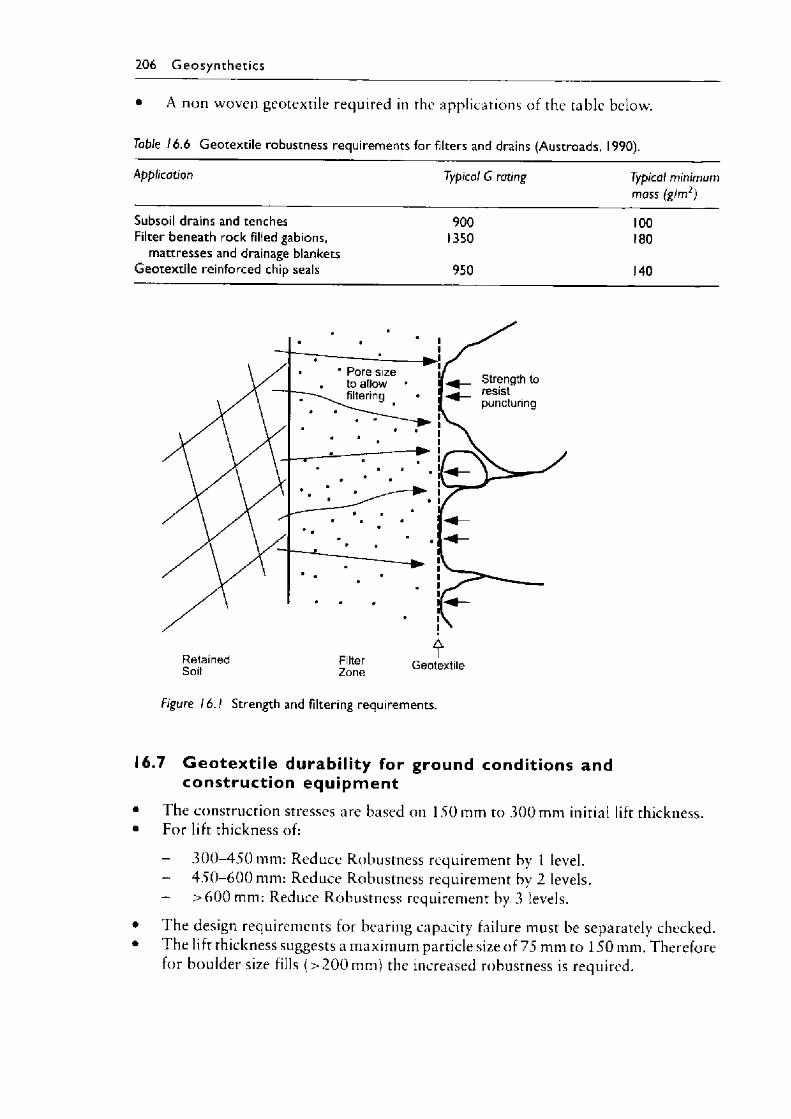
206 G e o s y n th e t ic s
A non woven geotextile required in the applications of the table below.
Table 16.6 Geotextile robustness requirements for filters and drains (Austroads, 1990).
Application Typical G rating Typical minimum mass (g/m2)
Subsoil drains and tenches 900 100Filter beneath rock filled gabions, 1350 180
mattresses and drainage blanketsGeotextile reinforced chip seals 950 140
Figure 16.1 Strength and filtering requirements.
16.7 G eotext i le durability for ground conditions and construction equipment
• The construction stresses are based on 150 mm to 300 mm initial lift thickness.• For lift thickness of:
- 3 0 0 - 4 5 0 mm: Reduce Robustness requirement by I level.- 4 5 0 - 6 0 0 mm: Reduce Robustness requirement by 2 levels.- > 6 0 0 mm: Reduce Robustness requirement by 3 levels.
• The design requirements for bearing capacity failure must be separately checked.• The lift thickness suggests a maximum particle size of 75 mm to 150 mm. Therefore
for boulder size fills ( > 2 0 0 mm) the increased robustness is required.
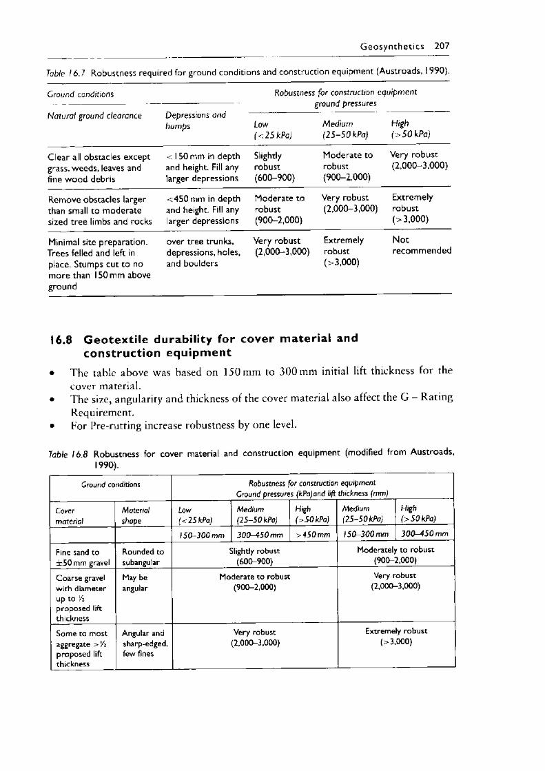
G e o s y n th e t ic s 207
Table 16 .7 Robustness required for ground conditions and construction equipment (Austroads, 1990).
Ground conditions Robustness for construction equipmentground pressures
Natural ground clearance Depressions and humps Low
(< 25 kPa)Medium (25-50 kPa)
High(> 5 0 kPa)
Clear all obstacles except grass, weeds, leaves and fine wood debris
< 150 mm in depth and height. Fill any larger depressions
Slightlyrobust(600-900)
Moderate torobust(900-2,000)
Very robust (2,000-3,000)
Remove obstacles larger than small to moderate sized tree limbs and rocks
<450 mm in depth and height. Fill any larger depressions
Moderate torobust(900-2,000)
Very robust (2,000-3,000)
Extremelyrobust(>3,000)
Minimal site preparation. Trees felled and left in place. Stumps cut to no more than 150 mm above ground
over tree trunks, depressions, holes, and boulders
Very robust (2,000-3,000)
Extremelyrobust(>3,000)
Notrecommended
16.8 Geotext i le durabil ity for cover materia l and construction equipment
• The table above was based on 150 mm to 300 mm initial lift thickness for the cover material.
• The size, angularity and thickness of the cover material also affect the G - Rating Requirement.
• For Pre-rutting increase robustness by one level.
Table 16.8 Robustness for cover material and construction equipment (modified from Austroads,1990).
Ground conditions Robustness for construction equipment Ground pressures (kPa)and lift thickness (mm)
Covermaterial
Materialshape
Low(<25kPa)
Medium (25-50 kPa)
High(>50kPa)
Medium (25-50 kPa)
High(>50 kPa)
150-300 mm 300-450 mm >450 mm 150-300 mm 300—450 mm
Fine sand to ± 5 0 mm gravel
Rounded to subangular
Slightly robust (600-900)
Moderately to robust (900-2,000)
C o a rse gravel w ith diameter up to Zt proposed lift thickness
May be angular
M oderate to robust (900-2,000)
Very robust (2,000-3,000)
Som e to m ost aggregate >'A proposed lift thickness
Angular and sharp-edged, few fines
Very robust (2,000-3,000)
Extrem ely robust (> 3,000)
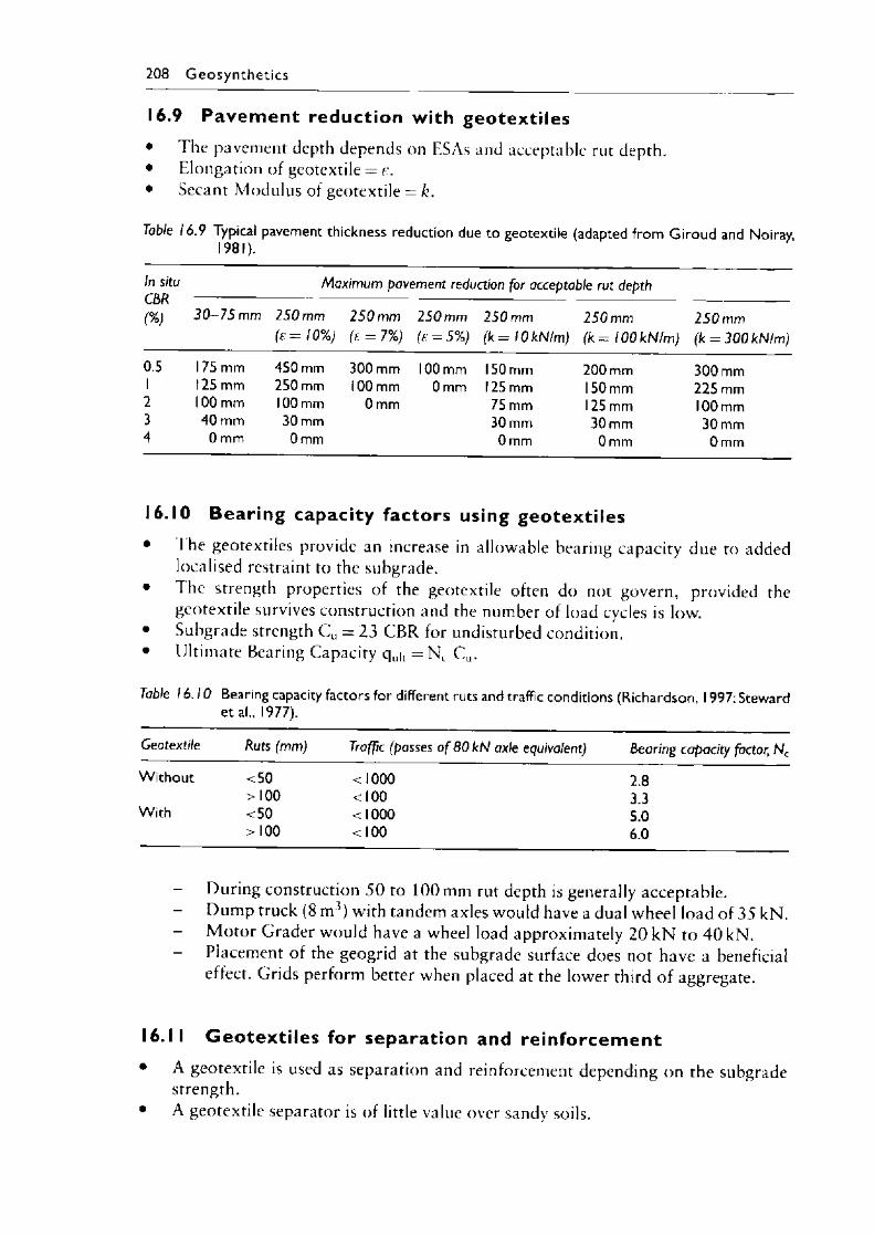
208 G e o s y n th e t ic s
16.9 Pavem ent reduction with geotextiles• The pavement depth depends on ESAs and acceptable rut depth.• Elongation of geotextile = e .• Secant Modulus of geotextile = k.
Table 16.9 Typical pavement thickness reduction due to geotextile (adapted from Giroud and Noiray, 1981).
In situ CBR(%)
Maximum pavement reduction for acceptable rut depth
3 0 -7 5 mm 250 mm (£ = 10%)
250 mm(s = 7%)
250 mm(e = 5%)
250 mm (k = lOkNIm )
250 mm ( k = lOOkN/m)
250 mm (k = 300kN/m )
0.5 175 mm 450 mm 300 mm 100 mm 150 mm 200 mm 300 mm1 125 mm 250 mm 100 mm 0 mm 125 mm 150 mm 225 mm2 100 mm 100 mm 0 mm 75 mm 125 mm 100 mm3 40 mm 30 mm 30 mm 30 mm 30 mm4 0 mm 0 mm 0 mm 0 mm 0 mm
16.10 Bearing capacity factors using geotextiles• The geotextiles provide an increase in allowable bearing capacity due to added
localised restraint to the subgrade.• I he strength properties of the geotextile often do not govern, provided the
geotextile survives construction and the number of load cycles is low.• Subgrade strength C u = 23 C BR for undisturbed condition.• Ultimate Bearing Capacity q u|t = Nc C u.
Table 16.10 Bearing capacity factors for different ruts and traffic conditions (Richardson, I 997: Steward et al„ 1977).
Geotextile Ruts (mm) Traffic (passes o f 80 kN axle equivalent) Bearing capacity factor, Nc
W ithout <50 <1000 2.8>100 <100 3.3
With <50 <1000 5.0>100 <100 6.0
- During construction 5 0 to 100 mm rut depth is generally acceptable.Dump truck ( 8 m ] ) with tandem axles would have a dual wheel load of 35 kN.
- M otor Grader would have a wheel load approximately 20 kN to 4 0 kN.- Placement of the geogrid at the subgrade surface does not have a beneficial
effect. Grids perform better when placed at the lower third of aggregate.
16.11 G eotext i les for separation and re inforcement• A geotextile is used as separation and reinforcement depending on the subgrade
strength.• A geotextile separator is of little value over sandy soils.
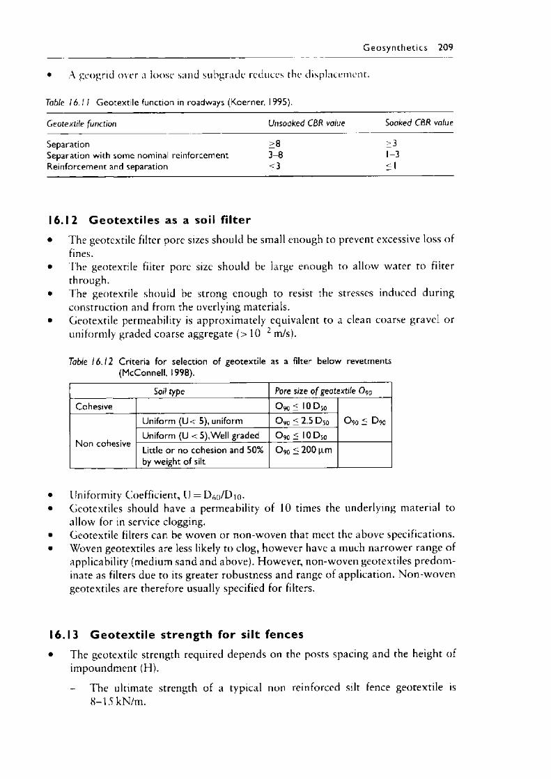
G eo syn th etics 209
• A geogrid over a loose sand subgrade redi
Table 16.11 Geotextile function in roadways (Koerner,
nces the displacement.
1995).
Geotextile function Unsoaked CBR value Soaked CBR value
Separation >8 >3Separation with some nominal reinforcement 3-8 1-3Reinforcement and separation <3 <1
16.12 Geotexti les as a soil filter• The geotextile filter pore sizes should be small enough to prevent excessive loss of
fines.• The geotextile filter pore size should be large enough to allow water to filter
through.• The geotextile should be strong enough to resist the stresses induced during
construction and from the overlying materials.• Geotextile permeability is approximately equivalent to a clean coarse gravel or
uniformly graded coarse aggregate ( > 1 0 2 m/s).
Table 16.12 Criteria for selection of geotextile as a filter below revetments (McConnell, 1998).
Soil type Pore size o f geotextile O90
Cohesive O 90 < 10 D 50
O 90 < D 90
Non cohesive
Uniform (U< 5), uniform O 90 5: 2.5 D 50
Uniform (U < 5),Well graded O 90 5: 10 D 50
Little or no cohesion and 50% by weight of silt
O 90 < 200 [im
• Uniformity Coefficient, U = D^/Dio*• Geotextiles should have a permeability of 10 times the underlying material to
allow for in service clogging.• Geotextile filters can be woven or non-woven that meet the above specifications.• Woven geotextiles are less likely to clog, however have a much narrower range of
applicability (medium sand and above). However, non-woven geotextiles predominate as filters due to its greater robustness and range of application. Non-woven geotextiles are therefore usually specified for filters.
16.13 Geotexti le strength for silt fences• The geotextile strength required depends on the posts spacing and the height of
impoundment (H).
The ultimate strength of a typical non reinforced silt fence geotextile is 8 - 1 5 kN/m.
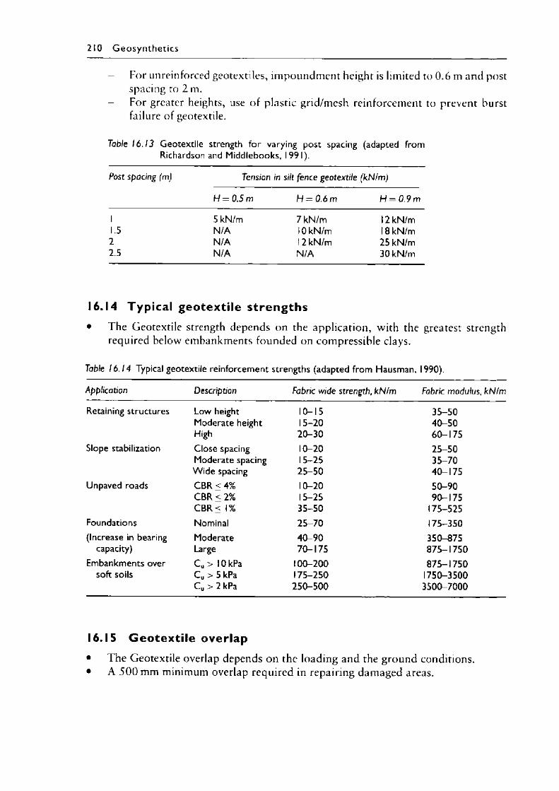
210 G e o s y n th e t ic s
For unreinforced geotextiles, impoundment height is limited to 0 .6 m and post spacing to 2 m. For greater heights, use of plastic grid/mesh reinforcement to prevent burst failure of geotextile.
Table 16.13 Geotextile strength for varying post spacing (adapted from Richardson and Middlebooks, 1991).
Post spacing (m) Tension in silt fence geotextile (kN/m)
H = 0.5 m H = 0.6 m H = 0 .9 m
1 5 kN/m 7 kN/m 12 kN/m1.5 N/A 10 kN/m 18 kN/m2 N/A 12 kN/m 25 kN/m2.5 N/A N/A 30 kN/m
16.14 Typical geotextile strengths• The Geotextile strength depends on the application, with the greatest strength
required below embankments founded on compressible clays.
Table 16.14 Typical geotextile reinforcement strengths (adapted from Hausman, 1990).
Application Description Fabric wide strength, kN/m Fabric modulus, kN/m
Retaining structures Low height 10-15 35-50Moderate height 15-20 40-50High 20-30 60-175
Slope stabilization Close spacing 10-20 25-50Moderate spacing 15-25 35-70Wide spacing 25-50 40-175
Unpaved roads CBR < 4% 10-20 50-90CBR < 2% 15-25 90-175CBR < 1% 35-50 175-525
Foundations Nominal 25-70 175-350(Increase in bearing Moderate 40-90 350-875
capacity) Large 70-175 875-1750Embankments over C u > 10 kPa 100-200 875-1750
soft soils Cu > 5 kPa 175-250 1750-3500C u > 2 kPa 250-500 3500-7000
16.15 G eotext i le overlap• The Geotextile overlap depends on the loading and the ground conditions.• A 5 0 0 mm minimum overlap required in repairing damaged areas.
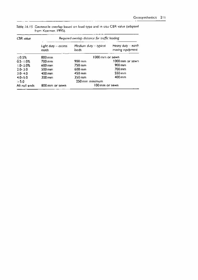
G e o s y n th e t ic s 2 1 I
Table 16.15 Geotextile overlap based on load type and in situ CBR value (adapted from Koerner, 1995).
CBR value Required overlap distance for traffic loading
Light duty - access roads
Medium duty loads
- typical Heavy duty - earth moving equipment
<0.5% 800 mm 1000 mm o r sewn0.5-1.0% 700 mm 900 mm 1000 mm or sewn1.0-2.0% 600 mm 750 mm 900 mm2.0-3.0 500 mm 600 mm 700 mm3.0—4.0 400 mm 450 mm 550 mm4.0-5.0 300 mm 350 mm 400 mm>5.0 250 mm minimumAll roll ends 800 mm or sewn 100 mm or sewn

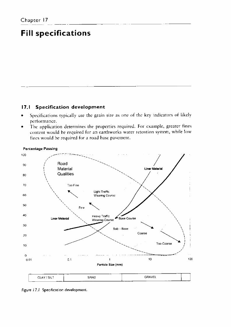
Chapter 17
Fill specifications
17.1 Specification development• Specifications typically use the grain size as one of the key indicators of likely
performance.• The application determines the properties required. For example, greater fines
content would be required for an earthworks water retention system, while low fines would be required for a road base pavement.
Percentage Passing
Particle S ize (mm)
CLAY / SILT SAND GRAVEL
Figure I 7. 1 Specification development.
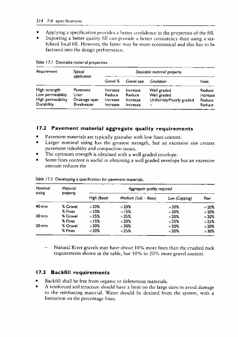
214 Fill spec if ica t io n s
• Applying a specification provides a better confidence in the properties of the fill.• Importing a better quality fill can provide a better consistency than using a sta
bilised local fill. However, the latter may be more economical and this has to be factored into the design performance.
Table 17.1 Desirable material properties.
Requirement Typicalapplication
Desirable material property
Gravel % Gravel size Gradation Fines
High strength Low permeability High permeability Durability
PavementLinerDrainage layer Breakwater
IncreaseReduceIncreaseIncrease
IncreaseReduceIncreaseIncrease
Well graded Well gradedUniformly/Poorly graded
ReduceIncreaseReduceReduce
17.2 Pavem ent m ateria l aggregate quality req u irem ents• Pavement materials are typically granular with low fines content.• Larger nominal sizing has the greatest strength, but an excessive size creates
pavement rideabilty and compaction issues.• The optimum strength is obtained with a well graded envelope.• Some fines content is useful in obtaining a well graded envelope but an excessive
amount reduces the
Table I 7.2 Developing a specification for pavement materials.
Nominal Material Aggregate quality requiredsizing property
High (Base) Medium (Sub - Base) Low (Capping) Poor
40 mm % Gravel >20% >20% >20% <20%% Fines <10% <15% <20% >20%
30 mm % Gravel >25% >25% >20% <20%% Fines <15% <20% <25% >25%
20 mm % Gravel >30% >30% >20% <20%% Fines <20% <25% <30% >30%
- Natural River gravels may have about 1 0 % more fines than the crushed rock requirements shown in the table, but 1 0 % to 2 0 % more gravel content.
17.3 Backfi ll requ irem ents• Backfill shall be free from organic or deleterious materials.• A reinforced soil structure should have a limit on the large sizes to avoid damage
to the reinforcing material. Water should be drained from the system, with a limitation on the percentage fines.
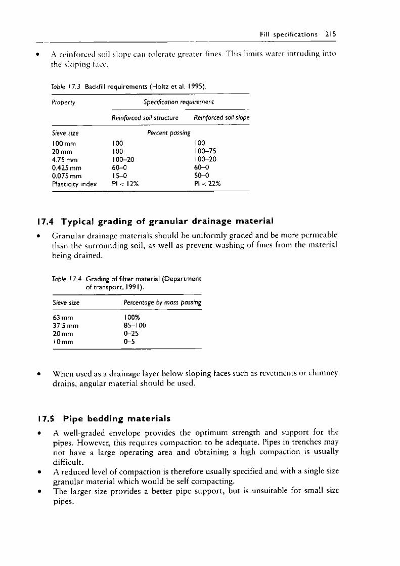
Fill sp ec if ica t io n s 215
• A r e i n f o r c e d soil s l o p e c a n t o l e r a te g r e a t e r fines. T h is l imits w a te r intrudi ng into
the s l o p i n g face.
Table 17.3 Backfill requirements (Holtz et al. 1995).
Property Specification requirement
Reinforced soil structure Reinforced soil slope
S/eve size Percent passing100 mm 100 10020 mm 100 100-754.75 mm 100-20 100-200.425 mm 60-0 60-00.075 mm 15-0 50-0Plasticity index PI < 12% PI < 22%
17.4 Typ ica l grading of g ranu lar drainage material• Granular drainage materials should be uniformly graded and be more permeable
than the surrounding soil, as well as prevent washing of fines from the material being drained.
Table I 7.4 Grading of filter material (Department of transport, 1991).
Sieve size Percentage by mass passing
63 mm 100%37.5 mm 85-10020 mm 0-2510 mm 0-5
• When used as a drainage layer below sloping faces such as revetments or chimney drains, angular material should be used.
17.5 Pipe bedding m ater ia ls• A well-graded envelope provides the optimum strength and support for the
pipes. However, this requires compaction to be adequate. Pipes in trenches may not have a large operating area and obtaining a high compaction is usually difficult.
• A reduced level of compaction is therefore usually specified and with a single size granular material which would be self compacting.
• The larger size provides a better pipe support, but is unsuitable for small size pipes.
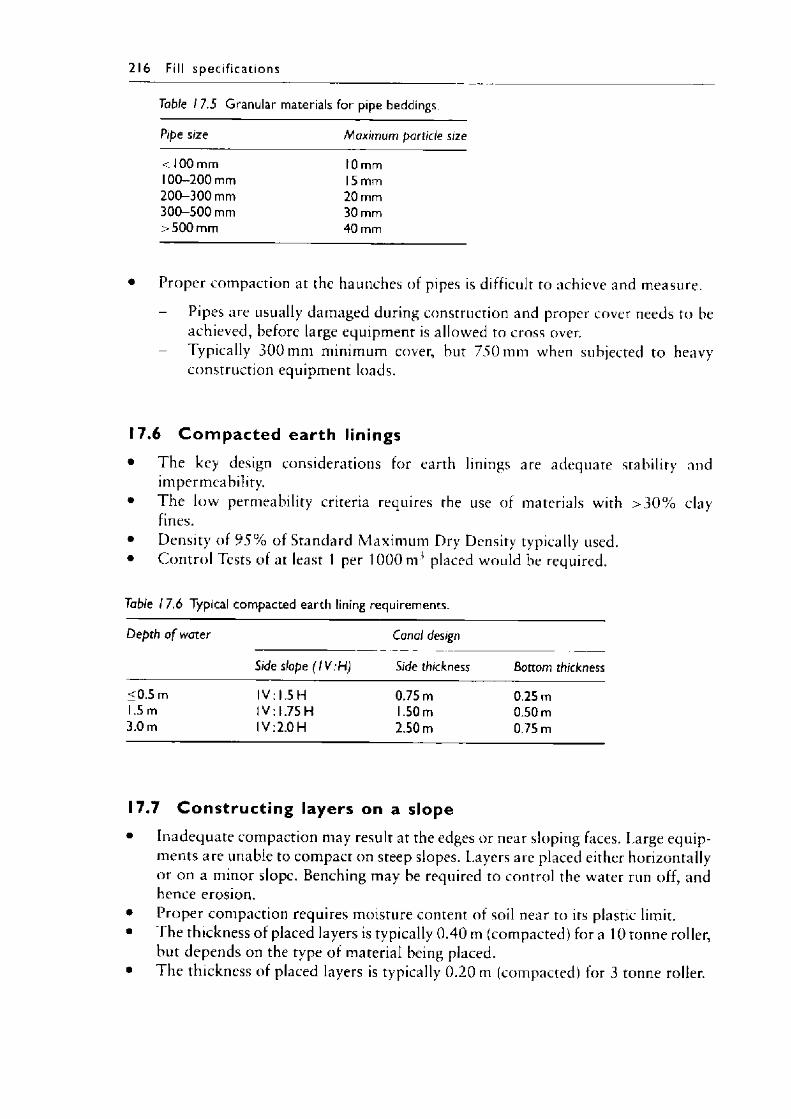
216 Fill sp ec if ica t io n s
Table I 7.5 Granular materials for pipe beddings.
Pipe size Maximum particle size
< 100 mm 10 mm100-200 mm 15 mm200-300 mm 20 mm300-500 mm 30 mm>500 mm 40 mm
Proper compaction at the haunches of pipes is difficult to achieve and measure.
- Pipes are usually damaged during construction and proper cover needs to be achieved, before large equipment is allowed to cross over.
- Typically 3 0 0 mm minimum cover, but 750 mm when subjected to heavy construction equipment loads.
17.6 C om p a cte d earth linings• The key design considerations for earth linings are adequate stability and
impermeability.• The low permeability criteria requires the use of materials with > 3 0 % clay
fines.• Density of 9 5 % of Standard Maximum Dry Density typically used.• Control Tests of at least 1 per 1000 nr' placed would be required.
Table I 7.6 Typical compacted earth lining requirements.
Depth o f water Canal design
Side slope ( I V : H ) Side thickness Bottom thickness
<0.5 m 1V : 1.5 H 0.75 m 0.25 m1.5 m 1V : 1.75 H 1.50 m 0.50 m3.0 m 1V :2.0 H 2.50 m 0.75 m
17.7 Constru ct ing layers on a slope• Inadequate compaction may result at the edges or near sloping faces. Large equip
ments are unable to compact on steep slopes. Layers arc placed either horizontally or on a minor slope. Benching may be required to control the water run off, and hence erosion.
• Proper compaction requires moisture content of soil near to its plastic limit.• The thickness of placed layers is typically 0 .4 0 m (compacted) for a 10 tonne roller,
but depends on the type of material being placed.• The thickness of placed layers is typically 0 .2 0 m (compacted) for 3 tonne roller.
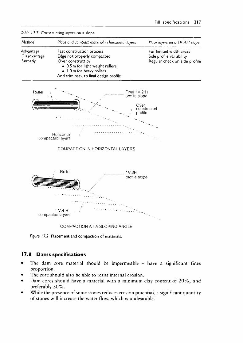
Fill sp ec if ica t io n s 217
Table I 7.7 Constructing layers on a slope.
Method Place and compact material in horizontal layers Place layers on a IV :4 H slope
AdvantageDisadvantageRemedy
Fast construction process Edge not properly compacted O ver construct by
• 0.5 m for light weight rollers• 1.0 m for heavy rollers
And trim back to final design profile
For limited width areas Side profile variability Regular check on side profile
Roller \ x ____ Final 1V:2 H/ profile slope
Overs x t— constructed
' • / profile. ^ ^
____ , ______________ .
Horizontal ____/compacted layers
C O M PA C TIO N IN H O R IZO N TA L L A Y E R S
j Roller _____________1V:2Hprofile slope
1 V :4 H J ..................... — ^compacted layers
C O M PA C TIO N A T A S LO P IN G A N G LE
Figure I 7.2 Placement and compaction of materials.
I 7.8 Dams specifications• The dam core material should be impermeable - have a significant fines
proportion.• The core should also be able to resist internal erosion.• Dam cores should have a material with a minimum clay content of 2 0 % , and
preferably 3 0 % .• While the presence of some stones reduces erosion potential, a significant quantity
of stones will increase the water flow, which is undesirable.
218 Fill spec if ica t ion s
Table I 7.8 Dam core material classification to minimise internal erosion.
Consideration Reduce erosion Erosion resistance
Criteria Rate of erosion Higher compacted Addition or inclusion Maximum stonedecreases with density reduces of stone chips size to allowincreasing plasticity Index (PI)
rate of erosion improves erosion resistance
compaction
Measure ideal PI = 15% to 20% D ry Density (DD) >98% (Standard proctor)
Stones = 10% to 20% Stone size = 2 mm to 60 mm
Fair PI > 12% D D > 95% Stones > 5% Stones < 25%
Stones < 100 mm
Poor PI < 12% D D < 95% Stones < 5% Stones > 100 mmVery poor PI < 10% D D < 90% Stones > 25% Stones > 120 mm
17.9 F requency of testing• T he frequency of testing is based on the size of the area and project, uniformity
o f material and overall importance of the layer being tested.
Table I 7.9 Guidelines to frequency of testing.
Test Field density Grading and plasticity index
Frequency for large scale operations
For selected material imported to site - Not less thana) 1 test per 1000m3, andb) 4 tests per visitc) 1 test per 250 mm layer per
material type per 4000 m2
For on site material imported - Not less thana) 1 test per 500 m \ andb) 3 tests per visitc) 1 test per 250 mm layer per
material type per 2000 m2
1 test per 2000 m’ at selected source before transporting to site.1 test per 1000 m3 for using locally available material on site
Frequency for medium scale operations eg residential lots
Not less thana) 1 test per 250 m \ andb) 2 tests per visit, andc) 1 test per 250 mm layer per
material type per 1000 m2
1 test per 500 m3 at selected source before transporting to site1 test per 250 m* for using locally available material on site
Frequency for small scale operations using small or hand operated equipment eg backfilling, confined operations, trenches
Not less thana) 1 test per 2 layers per 50 m2, andb) 1 test per 2 layers per 50 linear m
1 test per 100 m \ a t selected source before transporting to site1 test per 50 m3, for using locally available material on site
Fill sp e c if ica t io n s 219
17.10 Rock revetm ents• R o c k re vetm ents c a n be selected rock arm ou r, rip rap or s t one pi tching.
Table 17.10 Rock revetments (McConnell, 1998).
Revetment type Specification Porosity Thickness
Rip - Rap Rock armour
C W D 15 ^ 2 to 2.5 D 85/D ,5 - 1.25 to 1.75
35 to 40% 30 to 35%
2 to 3 stones/rock sizes thick 2 rock sizes thick
17.1 I Durabil ity• The degradable materials decompose when exposed to air, as they take on water.• Sedimentary rocks are the most common rock types, which degrade rapidly, such
as shales and mudstones.• Foliated Metamorphic rocks such as slate and phyllites are also degradable.
Table 17.11 Indicators of rock durability.
Test Strong and durable Weak and non durable - Soil like
Rock like behaviour in long term Soil like behaviour in the long term
Point load index >2 MPa <1 MPaFree swell <3% >5%Slake durability test >90 <60Jar slake test > 6 < 2Los angeles abrasion <25% >40%Weathering Fresh to slightly weathered Extremely weatheredR Q D >50% <25%
• Several o f the above indicators should be in place before classed as a likely non durable material.
17.12 Durabil ity of pavements• The pavement material is usually obtained from crushed aggregate.• The wearing and base courses would have a higher durability requirements than
the sub base.
Table I 7.12 Durability requirements for a pavement.
Parameter Wearingcourse
Basecourse
Sub base
Upper Lower
W ater absorption < 2 % <3% < 4% <5%Aggregate crushing value <25% <30% <35% <40%Los angeles abrasion <30% <35% <40% <45%Sodium sulphate soundness < 10% <15% < 20% <25% LossFlakiness index <35 <40 <40 <45Ten percent fines (Wet) >150 kN > 100 kN >75 kN >50 kNW et/Dry strength variation <30% <40% <50% <50%
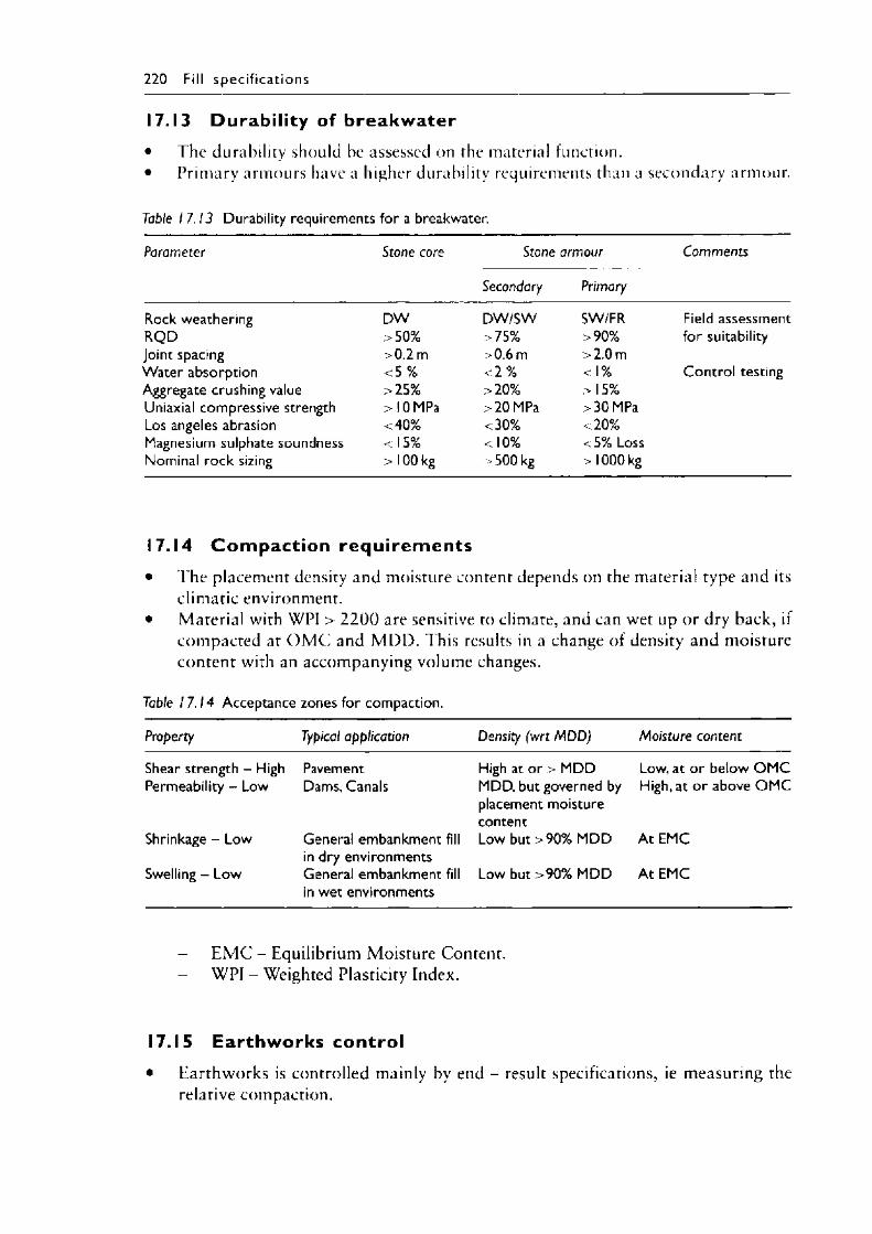
220 Fill spec if ica t ion s
17.13 Durabil ity of b reakw ater• The durability should be assessed on the material function.• Primary armours have a higher durability requirements than a secondary armour.
Table I 7.13 Durability requirements for a breakwater.
Parameter Stone core Stone armour
Secondary Primary
Comments
Rock weathering D W DW /SW SW/FR Field assessmentRQ D >50% >75% >90% for suitabilityJoint spacing > 0.2 m >0.6 m > 2.0 mWater absorption <5 % < 2 % < 1% Control testingAggregate crushing value >25% > 20% > 15%Uniaxial compressive strength > 10 MPa >20 MPa >30 MPaLos angeles abrasion <40% <30% < 20%Magnesium sulphate soundness < 15% < 10% <5% LossNominal rock sizing > 100 kg > 500 kg >10 0 0 kg
17.14 Com pact ion requ irem ents• The placement density and moisture content depends on the material type and its
climatic environment.• Material with WPI > 2 2 0 0 are sensitive to climate, and can wet up or dry back, if
compacted at O M C and M D D . This results in a change of density and moisture content with an accompanying volume changes.
Table 17.14 Acceptance zones for compaction.
Property Typical application Density (wrt MDD) Moisture content
Shear strength - High Permeability - Low
Shrinkage - Low
Swelling - Low
Pavement Dams, Canals
General embankment fill in dry environments General embankment fill in wet environments
High at or > MDD MDD, but governed by placement moisture contentLow but >90% MDD
Low but >90% MDD
Low, at or below O M C High, at or above O M C
At EM C
At EM C
- E M C - Equilibrium Moisture Content.- WPI - Weighted Plasticity Index.
17.15 Earthw orks control• Earthworks is controlled mainly by end - result specifications, ie measuring the
relative compaction.
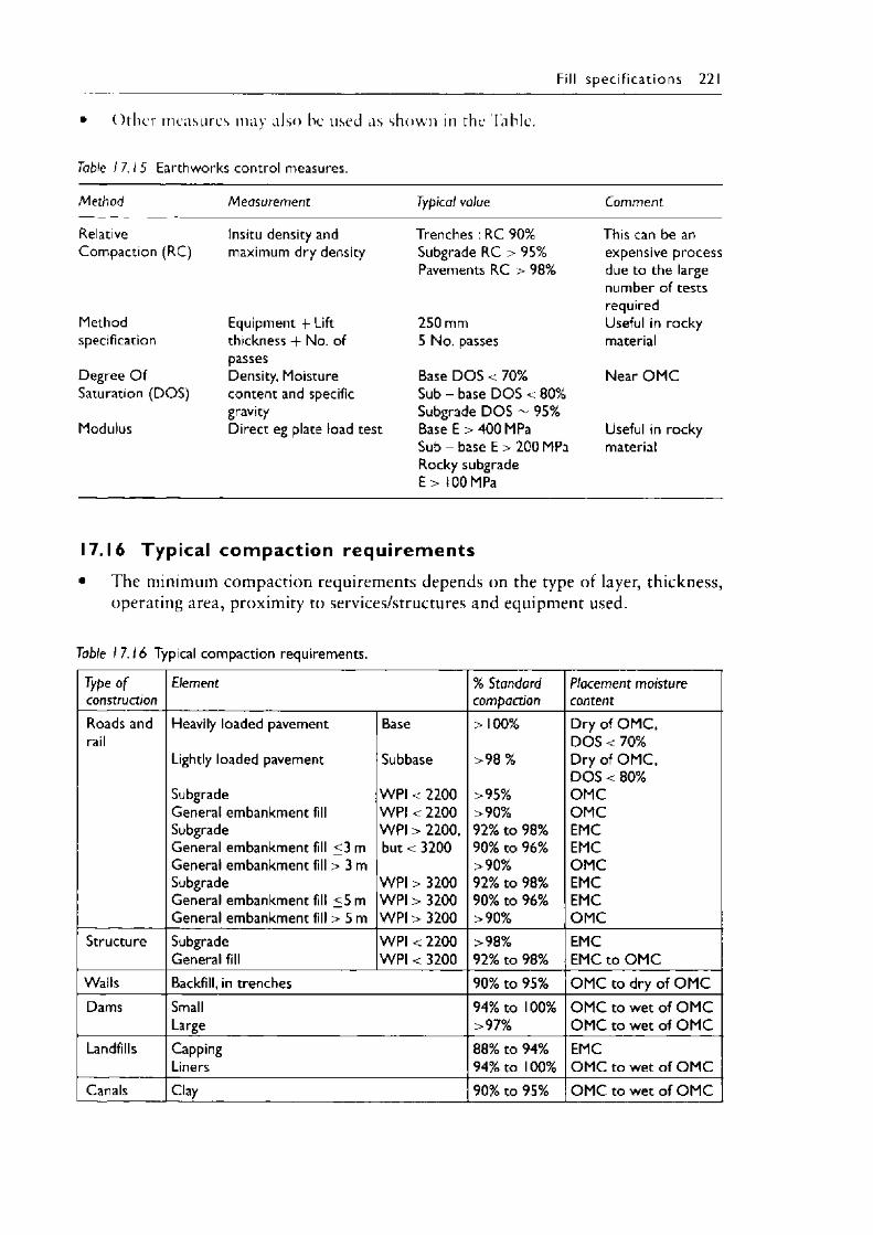
Fill sp ec if ic a t io n s 221
O t h e r measures may also he used as sh ow n in the Table .
Table 17.15 Earthworks control measures.
Method Measurement Typical value Comment
Relative Insitu density and Trenches : RC 90% This can be anCompaction (RC) maximum dry density Subgrade RC > 95%
Pavements RC > 98%expensive process due to the large number of tests required
Method Equipment -f Lift 250 mm Useful in rockyspecification thickness + No. of
passes5 No. passes material
Degree O f Saturation (DOS)
Density, Moisture content and specific gravity
Base D O S < 70%Sub - base D O S < 80% Subgrade D O S - 95%
Near O M C
Modulus Direct eg plate load test Base E > 400 MPa Sub - base E > 200 MPa Rocky subgrade E > 100 MPa
Useful in rocky material
17.16 Typical compaction requ irem ents• The minimum compaction requirements depends on the type of layer, thickness,
operating area, proximity to services/structures and equipment used.
Table I 7 .16 Typical compaction requirements.
Type o f Element % Standard Placement moistureconstruction compaction contentRoads and Heavily loaded pavement Base > 100% Dry of O M C,rail D O S < 70%
Lightly loaded pavement Subbase > 98% Dry of O M C,D O S < 80%
Subgrade W Pl < 2200 >95% O M CGeneral embankment fill W Pl < 2200 >90% O M CSubgrade W Pl > 2200, 92% to 98% EMCGeneral embankment fill <3m but < 3200 90% to 96% EMCGeneral embankment fill > 3 m >90% O M CSubgrade W Pl > 3200 92% to 98% EMCGeneral embankment fill <5m W Pl > 3200 90% to 96% EMCGeneral embankment fill > 5 m W Pl > 3200 >90% O M C
Structure Subgrade W Pl < 2200 >98% EMCGeneral fill W Pl < 3200 92% to 98% EMC to O M C
Walls Backfill, in trenches 90% to 95% O M C to dry of O M CDams Small 94% to 100% O M C to wet of O M C
Large >97% O M C to wet of O M CLandfills Capping 88% to 94% EMC
Liners 94% to 100% O M C to wet of O M CCanals Clay 90% to 95% O M C to wet of O M C
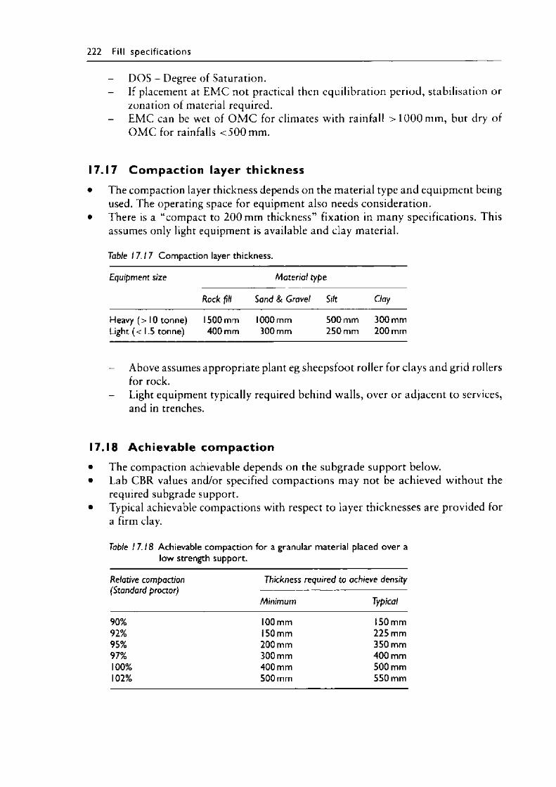
222 Fill spec if ica t ions
DOS - Degree of Saturation.- If placement at EM C not practical then equilibration period, stabilisation or
zonation of material required.- EM C can be wet of O M C for climates with rainfall > 1 0 0 0 mm, but dry of
O M C for rainfalls < 5 0 0 mm.
17.17 Com paction layer thickness• The compaction layer thickness depends on the material type and equipment being
used. The operating space for equipment also needs consideration.• There is a “compact to 2 0 0 mm thickness” fixation in many specifications. This
assumes only light equipment is available and clay material.
Table I 7.17 Compaction layer thickness.
Equipment size Material type
Rock fill Sand & Gravel Silt Clay
Heavy (> 10 tonne) 1500 mm 1000 mm 500 mm 300 mmLight (< 1.5 tonne) 400 mm 300 mm 250 mm 200 mm
Above assumes appropriate plant eg sheepsfoot roller for clays and grid rollers for rock.
- Light equipment typically required behind walls, over or adjacent to services, and in trenches.
17.18 Achievable compaction• The compaction achievable depends on the subgrade support below.• Lab CBR values and/or specified compactions may not be achieved without the
required subgrade support.• Typical achievable compactions with respect to layer thicknesses are provided for
a firm clay.
Table 17.18 Achievable compaction for a granular material placed over a low strength support.
Relative compaction (Standard proctor)
Thickness required to achieve density
Minimum Typical
90% 100 mm 150 mm92% 150 mm 225 mm95% 200 mm 350 mm97% 300 mm 400 mm100% 400 mm 500 mm102% 500 mm 550 mm

Fill spec if ica t ion s 223
• Lower strength subgrade materials would require an increased thickness specified.
The significant depths of material for the support can only apply to granular and rocky material with a suitable compaction equipment.
- Reduced thickness would require the use of a geotextile and/or capping layer to prevent punching and loss o f the material being compacted into the soft support.

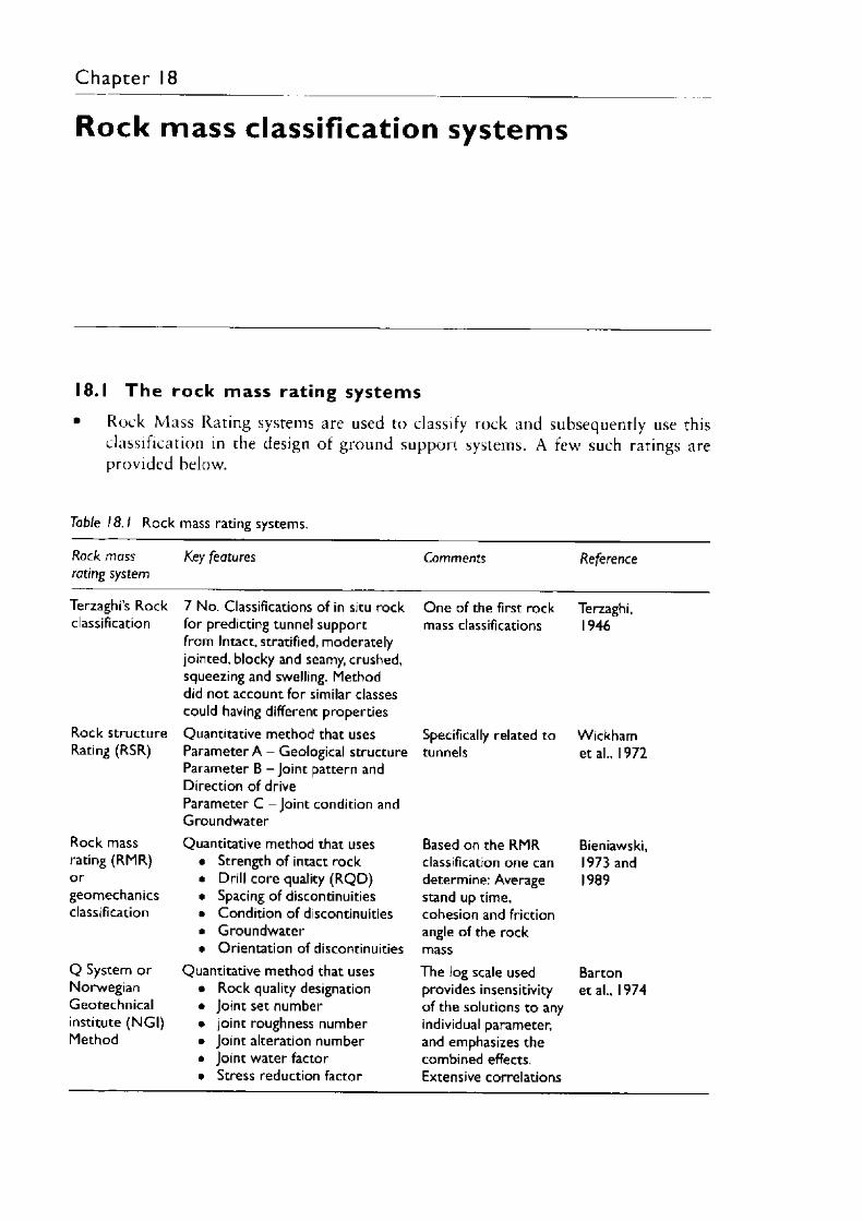
Ch ap ter 18
Rock mass classification systems
18.1 T h e rock mass rating systems• Rock M ass Rating systems are used to classify rock and subsequently use this
classification in the design of ground support systems. A few such ratings are provided below.
Table 18.1 Rock mass rating systems.
Rock mass Key features Comments Referencerating system
Terzaghi’s Rock 7 No. Classifications of in situ rock One of the first rock Terzaghi,classification for predicting tunnel support
from Intact, stratified, moderately jointed, blocky and seamy, crushed, squeezing and swelling. Method did not account for similar classes could having different properties
mass classifications 1946
Rock structure Quantitative method that uses Specifically related to WickhamRating (RSR) Parameter A - Geological structure
Parameter B - Joint pattern andDirection of driveParameter C - Joint condition andGroundwater
tunnels et al., 1972
Rock mass Quantitative method that uses Based on the RMR Bieniawski,rating (RMR) • Strength of intact rock classification one can 1973 andor • Drill core quality (RQ D) determine: Average 1989geomechanics • Spacing of discontinuities stand up time,classification • Condition of discontinuities
• Groundwater• Orientation of discontinuities
cohesion and friction angle of the rock mass
Q System or Quantitative method that uses The log scale used BartonNorwegian • Rock quality designation provides insensitivity et al., 1974Geotechnical • Joint set number of the solutions to anyinstitute (N GI) • joint roughness number individual parameter,Method • Joint alteration number
• Joint water factor• Stress reduction factor
and emphasizes the combined effects. Extensive correlations
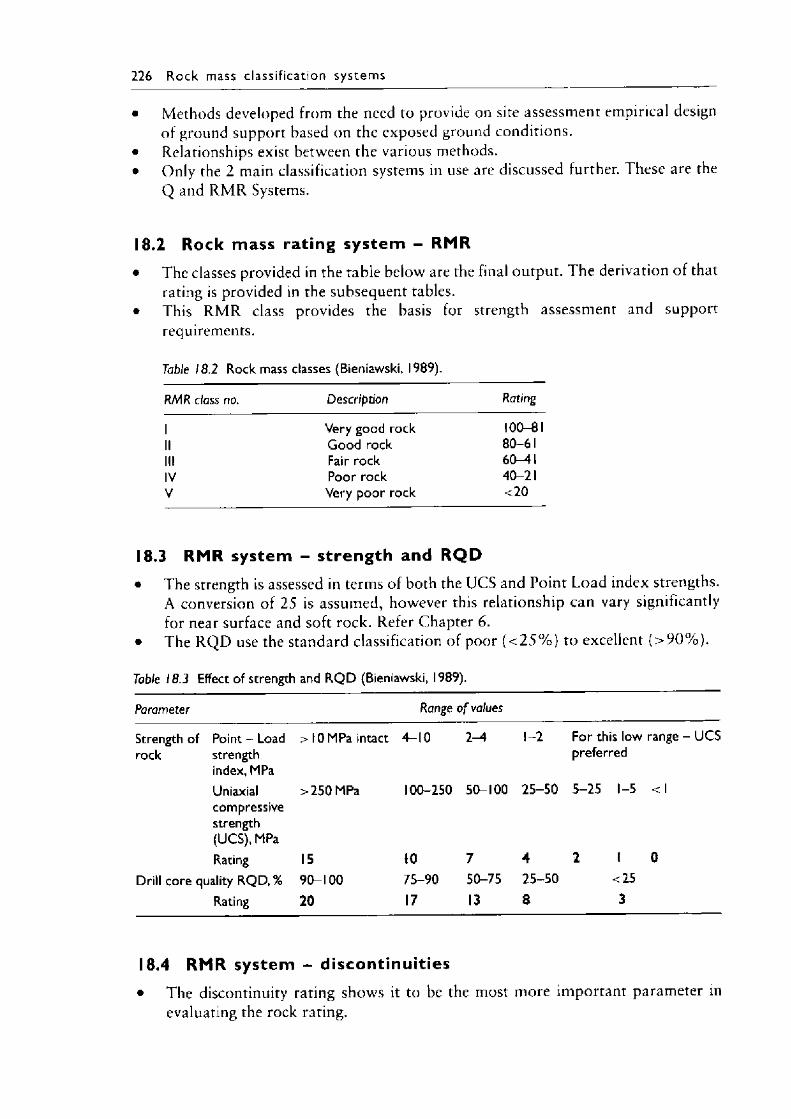
226 R o ck mass c lass i f ica t ion sy s te m s
• Methods developed from the need to provide on site assessment empirical designof ground support based on the exposed ground conditions.
• Relationships exist between the various methods.• Only the 2 main classification systems in use are discussed further. These are the
Q and R M R Systems.
18.2 Rock mass rating system - RMR• The classes provided in the table below are the final output. 1 he derivation of that
rating is provided in the subsequent tables.• This R M R class provides the basis for strength assessment and support
requirements.
Table 18.2 Rock mass classes (Bieniawski, 1989).
RMR class no. Description Rating
1 Very good rock 100-81II Good rock 80-61III Fair rock 60—41IV Poor rock 40-21V Very poor rock <20
18.3 RMR system - strength and R Q D• The strength is assessed in terms of both the UCS and Point Load index strengths.
A conversion of 25 is assumed, however this relationship can vary significantly for near surface and soft rock. Refer Chapter 6.
• The RQ D use the standard classification of poor ( < 2 5 % ) to excellent ( > 9 0 % ) .
Table 18.3 Effect of strength and R Q D (Bieniawski, 1989).
Parameter Range o f values
Strength of Point - Load rock strength
index, MPa
> 10 MPa intact 4-10 2-4 1 -2 For this low range - U CS preferred
Uniaxial >250 MPa 100-250 50-100 25-50 5-25 1-5 <1compressive strength (UCS), MPaRating 15 10 7 4 2 1 0
Drill core quality RQD, % 90-100 75-90 50-75 25-50 <25Rating 20 17 13 8 3
18.4 RMR system - discontinuities• The discontinuity rating shows it to be the most more important parameter in
evaluating the rock rating.
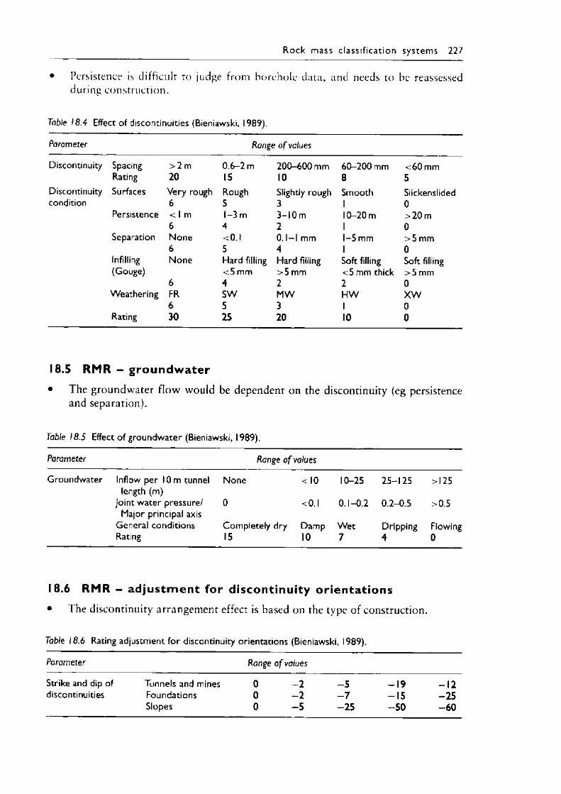
R o ck mass c la ss i f ica t ion sys tem s 227
• Persistence is difficult to judge from borehole data, and needs to be reassessed during construction.
Table 18.4 Effect of discontinuities (Bieniawski, 1989).
Parameter Range o f values
Discontinuity Spacing > 2m 0.6-2 m 200-600 mm 60-200 mm <60 mmRating 20 15 10 8 5
Discontinuity Surfaces Very rough Rough Slightly rough Smooth Slickenslidedcondition 6 5 3 I 0
Persistence < I m I-3 m 3-10 m 10-20 m >20m6 4 2 I 0
Separation None <0.1 0 .1 -lm m 1-5 mm >5 mm6 5 4 I 0
Infilling None Hard filling Hard filling Soft filling Soft filling(Gouge) <5 mm >5 mm <5 mm thick >5 mm
6 4 2 2 0Weathering FR SW MW H W X W
6 5 3 I 0Rating 30 25 20 10 0
18.5 RMR - groundwater• The groundwater flow would be dependent on the discontinuity (eg persistence
and separation).
Table 18.5 Effect of groundwater (Bieniawski, 1989).
Parameter Range o f values
Groundwater Inflow per 10 m tunnel None < 10 10-25 25-125 >125length (m)
Joint water pressure/ 0 <0.1 0. 1- 0.2 0.2- 0 .5 >0.5Major principal axis
General conditions Completely dry Damp Wet Dripping FlowingRating 15 10 7 4 0
18.6 RMR - ad justm ent for discontinuity orientations• The discontinuity arrangement effect is based on the type of construction.
Table 18.6 Rating adjustment for discontinuity orientations (Bieniawski, 1989).
Parameter Range o f values
Strike and dip of Tunnels and mines 0 - 2 - 5 - 1 9 - 1 2discontinuities Foundations 0 - 2 - 7 -1 5 -2 5
Slopes 0 - 5 - 2 5 - 5 0 - 6 0
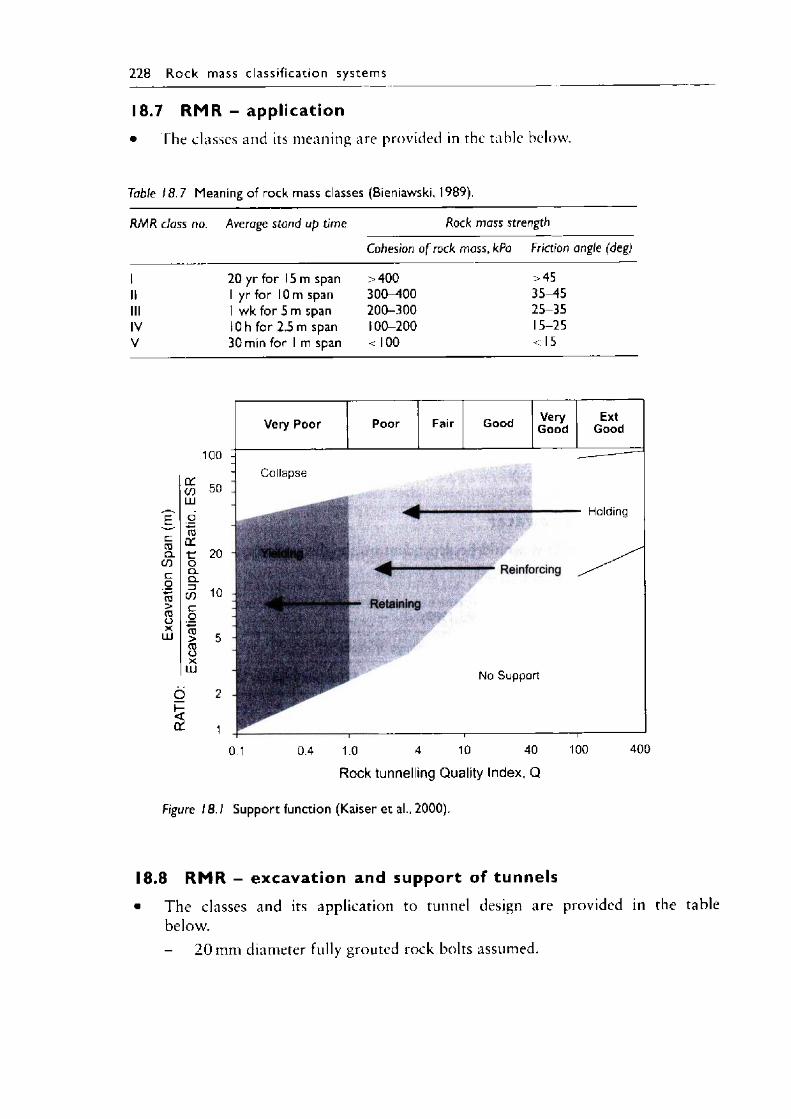
228 R o c k mass c la ss i f ica t io n sys tem s
18.7 RMR - application• The classes and its meaning are provided in the table below.
Table 18 .7 Meaning of rock mass classes (Bieniawski, 1989).
RMR class no. Average stand up time Rock mass strength
Cohesion o f rock mass, kPa Friction angle (deg)
1 20 yr for 15m span >400 >45II 1 yr for 10 m span 300—400 35—45III 1 wk for 5 m span 200-300 25-35IV 10 h for 2.5 m span 100-200 15-25V 30 min for 1 m span <100 <15
100
c03CLCOco■4—'03>03OX
LU
CO 50
03trtroQ.Q.DCOco03>03OX
LU
20
10
O
Very Poor Poor Good VeryGood
ExtGood
Collapse
No Support
Holding
Rock tunnelling Quality Index, Q
Figure 1 8 .1 Support function (Kaiser et al., 2000).
18.8 RMR - excavation and support of tunnels• The classes and its application to tunnel design are provided in the table
below.
- 2 0 mm diameter fully grouted rock bolts assumed.
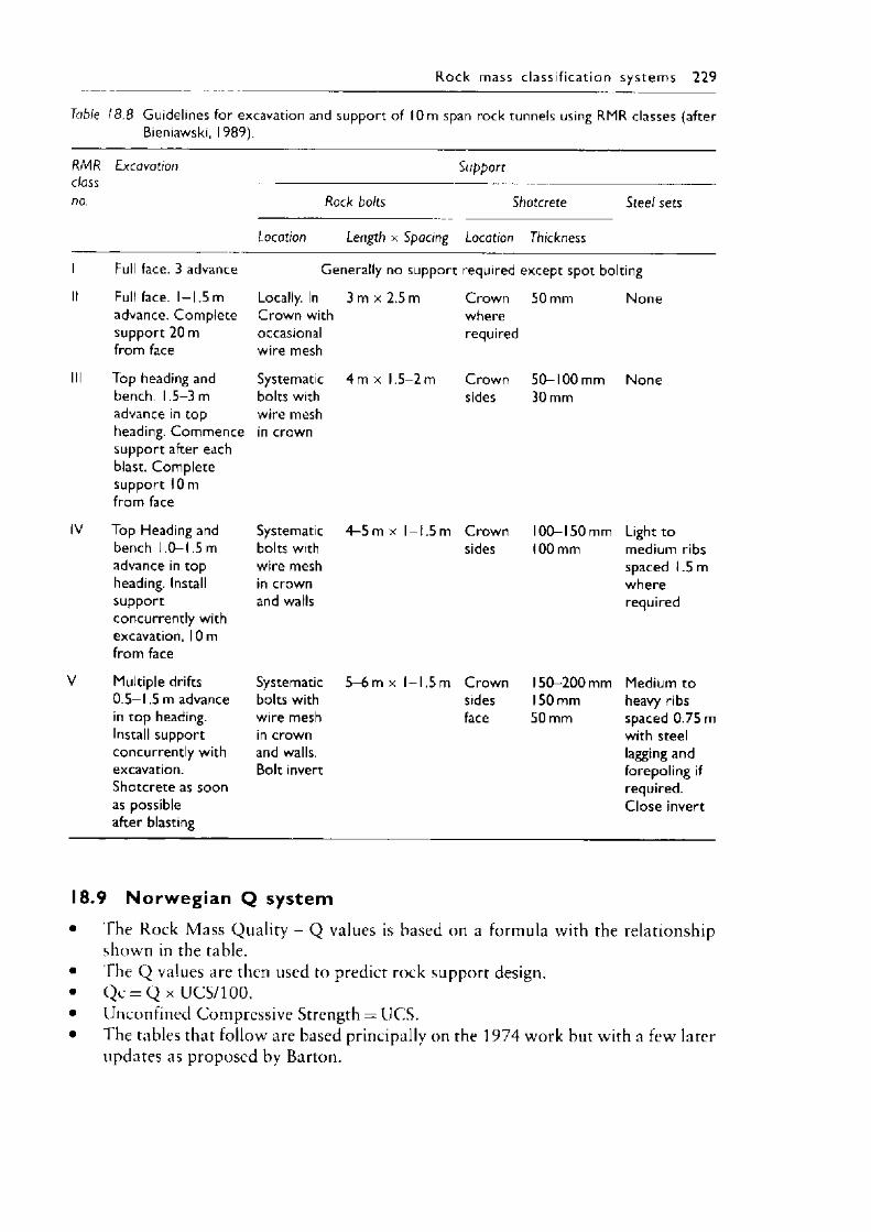
R ock mass c lass i f ica t ion sys tem s 229
Table 18.8 Guidelines for excavation and support of 10 m span rock tunnels using RMR classes (after Bieniawski, 1989).
RMR Excavationclassno.
Support
Rock bolts Shotcrete Steel sets
Location Length x Spacing Location Thickness
IV
Full face. 3 advance Generally no support required except spot bolting
Full face. 1-1.5 m Locally. Inadvance. Complete Crown witsupport 20 m occasionalfrom face wire mesh
Top heading and Systematicbench. 1.5-3 m bolts withadvance in top wire meshheading. Commence in crownsupport after eachblast. Completesupport 10 mfrom face
Top Heading and Systematicbench 1.0-1.5 m bolts withadvance in top wire meshheading. Install in crownsupport and wallsconcurrently withexcavation, 10 mfrom face
Multiple drifts Systematic0.5-1.5 m advance bolts within top heading. wire meshInstall support in crownconcurrently with and walls.excavation. Bolt invertShotcrete as soonas possibleafter blasting
3 m x 2.5 m
4 m x 1.5-2 m
Crownwhererequired
Crownsides
4-5 m x l - l .5 m Crownsides
5-6 m x I - 1.5 m Crownsidesface
50 mm
50-100 mm 30 mm
None
None
10 0 - 150 mm 100 mm
Light to medium ribs spaced 1.5 m where required
50-200 mm Medium to150 mm 50 mm
heavy ribs spaced 0.75 m with steel lagging and forepoling if required. Close invert
18.9 N o rw e g ia n Q sys tem• I he R o c k M a s s Q ua l i ty - Q values is based on a fo rm ula with the r e l a t i o n sh ip
s h o w n in the table.• T h e Q values are then used to predict ro ck s u pp or t design.• Q c = Q x U C S / 1 0 0 .• U n c o n f i n e d C o m p r e s s iv e Strength = U C S .• T h e tabl es th at fo l lo w are based pr incipally on the 1 9 7 4 w o r k but with a few later
u pd ate s as p ro p o se d by B art on .
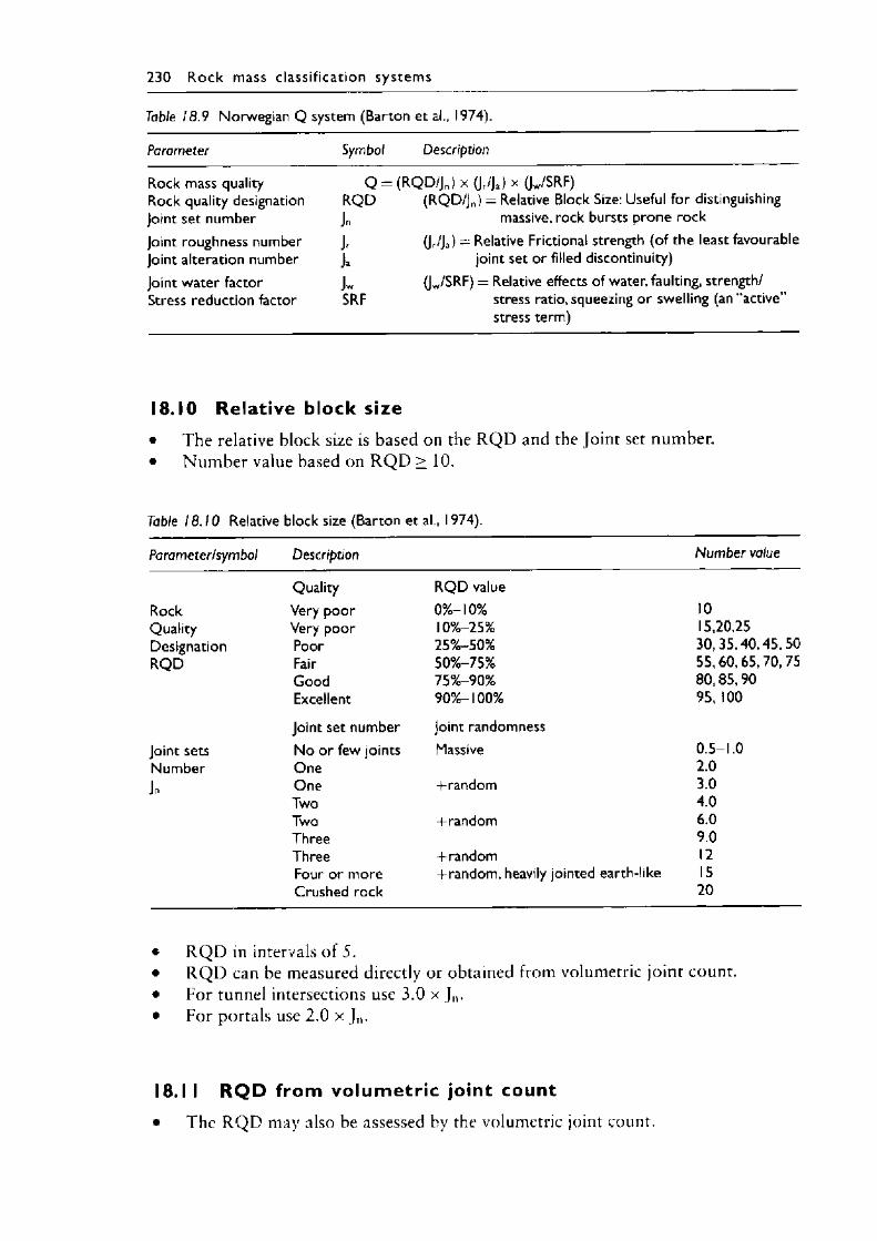
230 R o c k mass c lass i f ica t ion sys tem s
Table 18.9 Norwegian Q system (Barton et al., 1974).
Parameter Symbol Description
Rock mass quality Q = (RQ D /JJ x (Jr/Ja) x (JW/SRF)Rock quality designation RQ D (RQ D /JJ = Relative Block Size: Useful for distinguishingJoint set number Jn massive, rock bursts prone rockJoint roughness number Jr (Jr/Ja) = Relative Frictional strength (of the least favourableJoint alteration number Ja joint set or filled discontinuity)Joint water factor Jw (JW/SRF) = Relative effects of water, faulting, strength/Stress reduction factor SRF stress ratio, squeezing or swelling (an “active”
stress term)
18.10 R e la t ive block s ize• T h e relative b lock size is ba sed on the R Q D and the J o i n t set n um b e r .• N u m b e r value based on R Q D > 10.
Table 18.10 Relative block size (Barton et al., 1974).
Parameter/symbol Description Number value
Quality R Q D valueRock Very poor 0°/o-l0°/o 10Quality Very poor IO°/o-25% 15,20,25Designation Poor 25%-50°/o 30,35,40,45,50R Q D Fair 50%-75% 55,60,65,70, 75
Good 75°/o-90% 80,85,90Excellent 90%-100% 95, 100
Joint set number Joint randomnessJoint sets No or few joints Massive 0.5-1.0Number One 2.0Jn One + random 3.0
Two 4.0Two + random 6.0Three 9.0Three + random 12Four or more -f-random, heavily jointed earth-like 15Crushed rock 20
• R Q D in intervals o f 5.• R Q D ca n be measured direct ly or o b ta in e d fr o m volu m etr ic j o i n t c o u n t .• F o r tunn el intersect ions use 3 . 0 x J n.• F o r po rta l s use 2 . 0 x J n.
18.1 I R Q D from v o lu m e t r i c jo int count• T h e R Q D m a y also be assessed by the v o lu m et r i c jo int c o u n t .
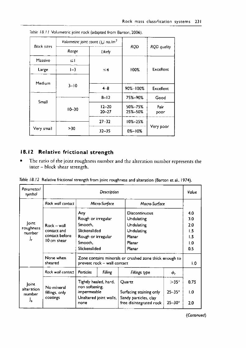
R o ck mass c lass i f ica t ion sy s te m s 231
Table 18 .11 Volumetric joint rock (adapted from Barton, 2006).
Block sizesVolumetric joint count (Jv) no./m3
RQD RQD qualityRange Likely
Massive <1
Large 1-3 <4 100% Excellent
Medium 3-10 4-8 90%-100% Excellent
8-12 75%-90% GoodSmall
10-30 12-2020-27
50%-75%25%-50%
Fairpoor
27-32 10%-25%Very poorVery small >30 32-35 0 % -10%
18.12 Re lat ive fr ict ional s trength• T h e ra t io o f the jo in t ro ugh ness n u m b e r and the a l te rat ion n u m b e r represents the
inter - b lo ck shear s trength.
Table 18 .12 Relative frictional strength from joint roughness and alteration (Barton et al., 1974).
Parameter/ symbol Description Value
Jointroughness
numberlr
Rock wall contact Micro-Surface Macro-Surface
4.03.02.01.51.5 1.0 0.5
Rock - wall contact and contact before 10 cm shear
AnyRough or irregularSmooth,SlickenslidedRough or irregularSmooth,Slickenslided
DiscontinuousUndulatingUndulatingUndulatingPlanarPlanarPlanar
None when sheared
Zone contains minerals or crushed zone thick enough to prevent rock - wall contact 1.0
Jointalterationnumber
Ja
Rock wall contact Particles Filling Fillings type 4>r
0.75
1.0
2.0
No mineral fillings, only coatings
Tightly healed, hard, non softening, impermeable Unaltered joint walls, none
Quartz
Surfacing staining only Sandy particles, clay free disintegrated rock
> 35°
25-35°
25-30°
(Continued)
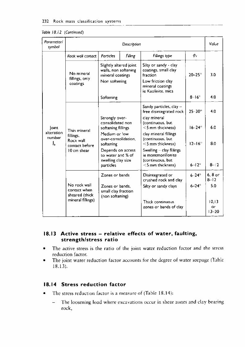
232 R o c k mass c lass i f ica t ion sys tem s
Table 18.12 (Continued)
Parameter/symbol
Description Value
Rock wall contact Particles Filling Fillings type <Pr
No mineral fillings, only coatings
Slightly altered joint walls, non softening mineral coatings Non softening
Softening
Silty or sandy - clay coatings, small clay fractionLow friction clay mineral coatings ie Kaolinite, mica
20-25°
8-16°
3.0
4.0
Jointalterationnumber
k
Thin mineral fillings.Rock wall contact before 10 cm shear
Strongly overconsolidated non softening fillings Medium or low over-consolidation, softeningDepends on access to water and % of swelling clay size particles
Sandy particles, clay - free disintegrated rockclay mineral (continuous, but <5 mm thickness) clay mineral fillings (continuous, but <5 mm thickness)Swelling - clay fillings ie montmorillonite (continuous, but <5 mm thickness)
25-30°
16-24°
12-16°
6-12°
4.0
6.0
8.0
8-12
No rock wall contact when sheared (thick mineral fillings)
Zones or bands
Zones or bands, small clay fraction (non softening)
Disintegrated or crushed rock and clay Silty or sandy clays
Thick continuous zones or bands of clay
6-24°
6-24°
6, 8 or 8-12
5.0
10,13or
13-20
18.13 Act ive stress - relative effects of water , faulting, strength/stress ratio
• The active stress is the ratio of the joint water reduction factor and the stress reduction factor.
• The joint water reduction factor accounts for the degree of water seepage (Table 18.13).
18.14 Stress reduction factor• The stress reduction factor is a measure of (Table 1 8.14):
The loosening load where excavations occur in shear zones and clay bearing rock,
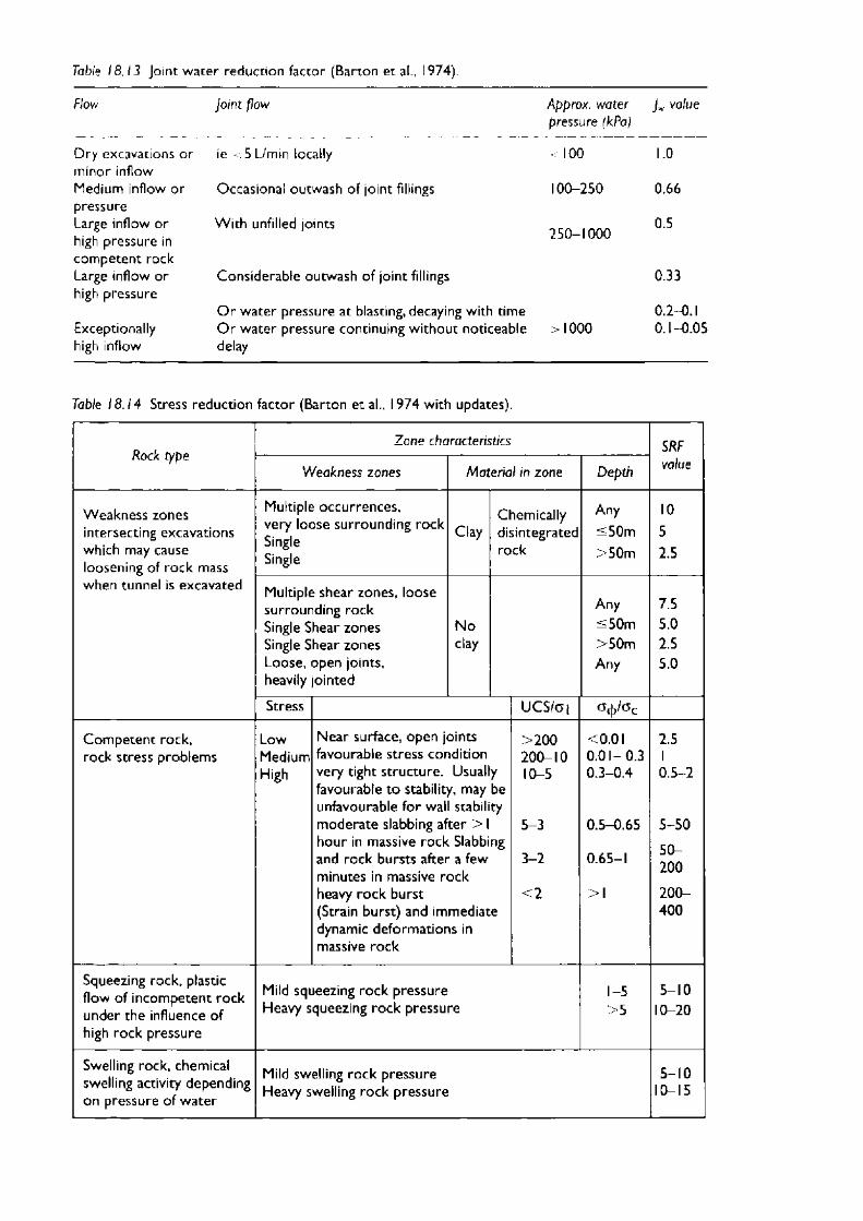
Table 18.13 Joint water reduction factor (Barton et al., 1974).
Flovv Joint flow
Dry excavations or ie 5 L/min locally minor inflow Medium inflow or pressure Large inflow or high pressure in competent rock Large inflow or high pressure
Exceptionally high inflow
Occasional outwash of joint fillings
With unfilled joints
Considerable outwash of joint fillings
Approx. water Jw value pressure (kPa)
100
100-250
250-1000
O r water pressure at blasting, decaying with timeO r water pressure continuing without noticeable > 1000delay
1.0
0.66
0.5
0.33
0 . 2- 0 . 1 0.1-0.05
Table 18.14 Stress reduction factor (Barton et al., 1974 with updates).
Rock typeZone characteristics SRF
valueWeakness zones Material in zone Depth
Weakness zones intersecting excavations which may cause loosening of rock mass when tunnel is excavated
Multiple occurrences,very loose surrounding rockSingleSingle
ClayChemicallydisintegratedrock
Any<50m>50m
1052.5
Multiple shear zones, loose surrounding rock Single Shear zones Single Shear zones Loose, open joints, heavily jointed
Noclay
Any<50m>50mAny
7.55.02.55.0
Stress UCS/C7| °c|A*C
Competent rock, rock stress problems
LowMediumHigh
Near surface, open joints favourable stress condition very tight structure. Usually favourable to stability, may be unfavourable for wall stability moderate slabbing after > 1 hour in massive rock Slabbing and rock bursts after a few minutes in massive rock heavy rock burst (Strain burst) and immediate dynamic deformations in massive rock
>200200-1010-5
5-3
3-2
< 2
<0.01 0.01-0.3 0.3-0.4
0.5-0.65
0.65-1
>1
2.510.5-2
5-5050-200200-400
Squeezing rock, plastic flow of incompetent rock under the influence of high rock pressure
Mild squeezing rock pressure Heavy squeezing rock pressure
1-5>5
5-1010-20
Swelling rock, chemical swelling activity depending on pressure of water
Mild swelling rock pressure Heavy swelling rock pressure
5-1010-15
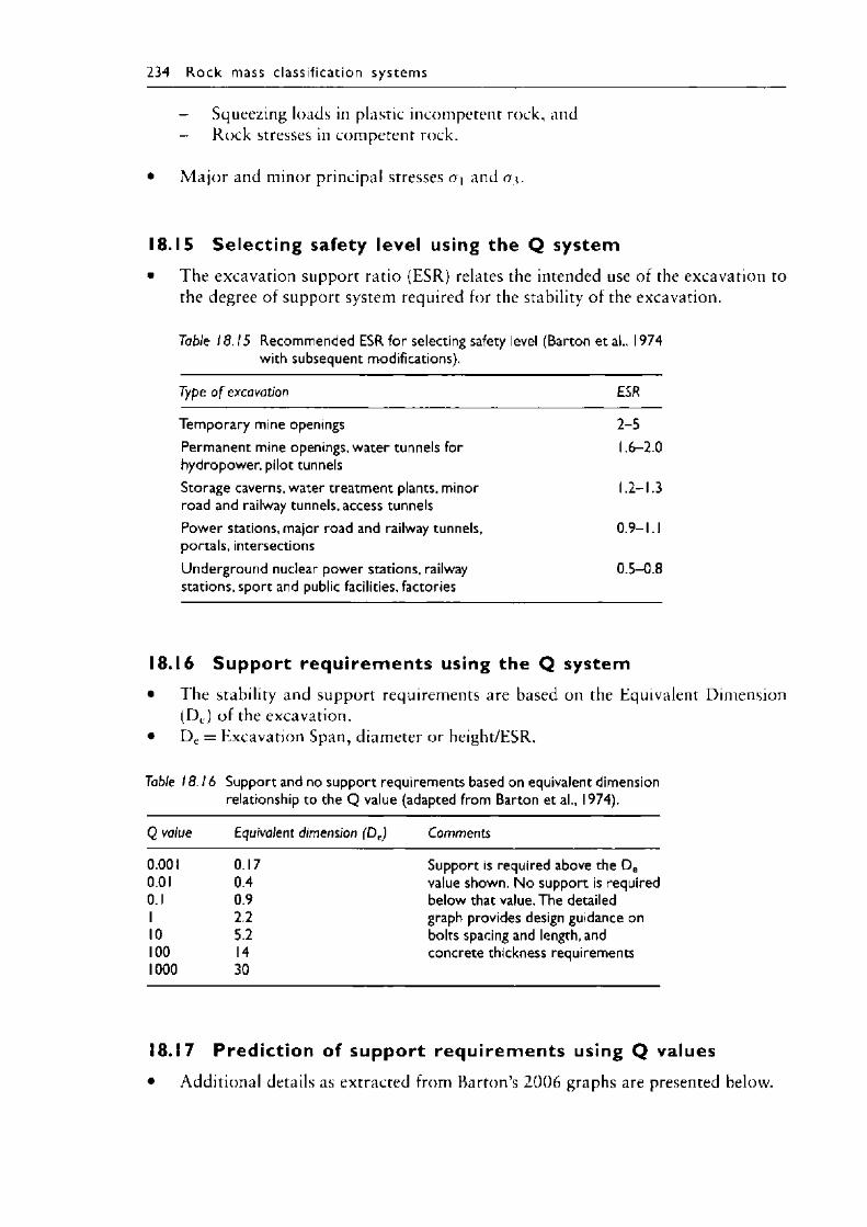
234 R o c k mass c lass i f ica t ion sys tem s
- Squeezing loads in plastic incompetent rock, and- Rock stresses in competent rock.
• M ajor and minor principal stresses a\ and a *.
18.15 Selecting safety level using the Q system• The excavation support ratio (ESR) relates the intended use of the excavation to
the degree of support system required for the stability of the excavation.
Table 18.15 Recommended ESR for selecting safety level (Barton et al., 1974 with subsequent modifications).
Type o f excavation ESR
Temporary mine openings 2-5Permanent mine openings, water tunnels for hydropower, pilot tunnels
1.6-2.0
Storage caverns, water treatment plants, minor road and railway tunnels, access tunnels
1.2-1.3
Power stations, major road and railway tunnels, portals, intersections
0 .9 - l.l
Underground nuclear power stations, railway stations, sport and public facilities, factories
0.5-0.8
18.16 Support requ irem ents using the Q system• T he stability and support requirements are based on the Equivalent Dimension
(D c) o f the excavation.• De = Excavation Span, diameter or height/ESR.
Table 18 .16 Support and no support requirements based on equivalent dimension relationship to the Q value (adapted from Barton et al., 1974).
Q value Equivalent dimension (De) Comments
0.001 0.17 Support is required above the D e0.01 0.4 value shown. No support is required0.1 0.9 below that value. The detailed1 2.2 graph provides design guidance on10 5.2 bolts spacing and length, and100 14 concrete thickness requirements1000 30
18.17 Predict ion of support requ irem ents using Q values• Additional details as extracted from Barton’s 2 0 0 6 graphs are presented below.
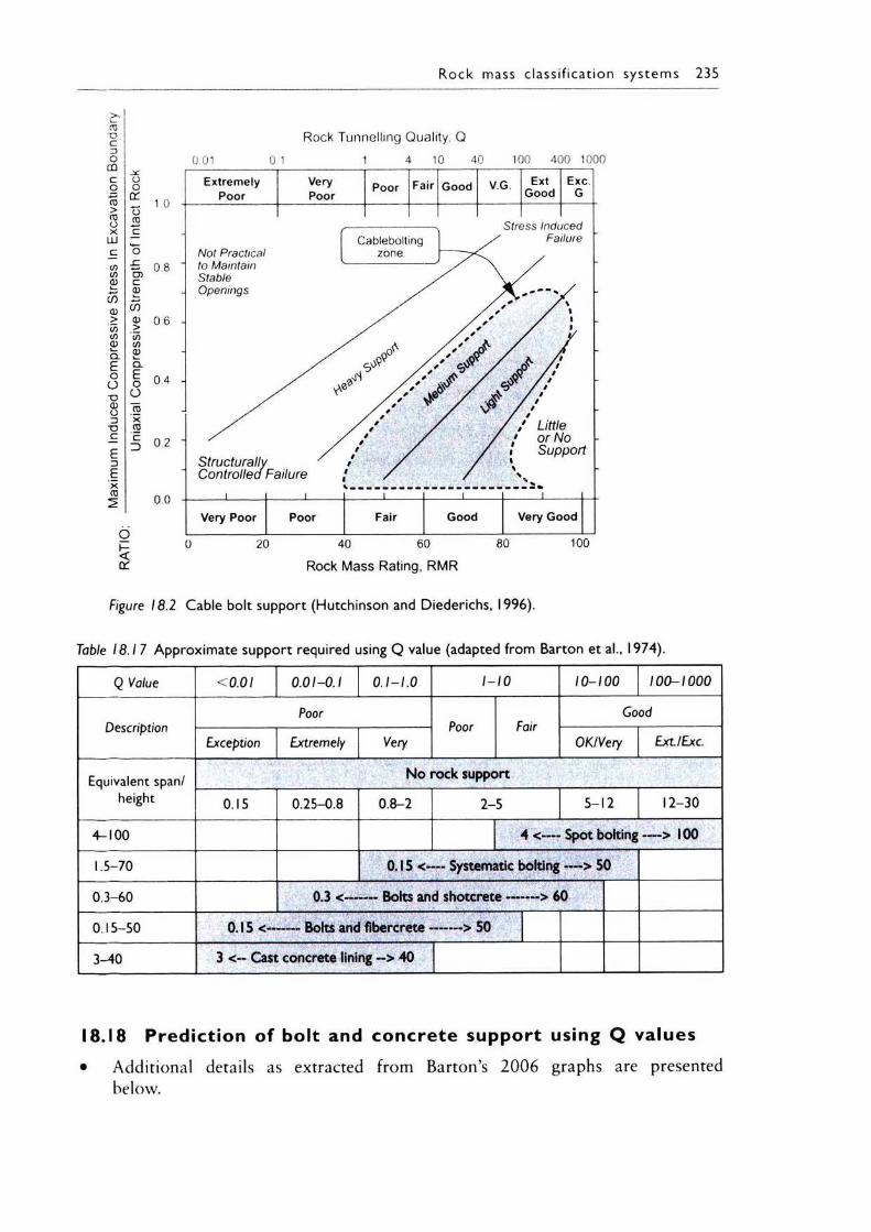
R o ck mass c la ss i f ica t ion sy s te m s 235
(f)<D>to(/)Q)Q.EoO
0.01
Rock Tunnelling Quality, Q0 1 1 4 10 40 100 400 1000
oo 1.0oegc
^ 0 U)cCD
0.6
0.4
0.2
0.0
Figure 18.2 Cable bolt support (Hutchinson and Diederichs, 1996).
Table 18.17 Approximate support required using Q value (adapted from Barton et al., 1974).
Q Value < 0.01 0.01-0.1 O.I-I.O 1-10 10-100 100-1000
DescriptionPoor
Poor FairGood
Exception Extremely Very OKIVery ExtlExc.
Equivalent span/ height
No rock support
0.15 0.25-0.8 0.8-2 2-5 5-12 12-30
4 - 100 4 <— Spot bolting — > 100
1.5-70 0.15 <— Systematic bolting — > 50
0.3-60 0.3 <------Bolts and shotcrete-------> 60
0 .15-50 0.15 <------Bolts and flbercrete-------> 50
3-40 3 <~ Cast concrete lining ~> 40
18.18 Predict ion of bolt and concrete support using Q values• Additional details as extracted from Barton’s 2 0 0 6 graphs are presented
below.
E x tre m e lyP o o r
VeryPo o r
P o o r G o o d ExtG o o d
0 20 40 60 80 100Rock Mass Rating, RMR
Cableboltingzone
Structurally Controlled Failure
Little or NoSupport
V e ry P o o r Po o r G o o d V e ry G o o d
Not Practical to Maintain Stable Openings
Stress Induced Failure
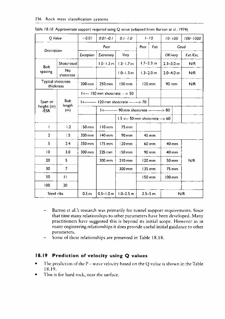
236 R o c k mass c lass i f ica t ion sys tem s
Table 18.18 Approximate support required using Q value (adapted from Barton at al., 1974).
Q Value <0.01 0 .01-0 .1 O .I- I .O 1-10 10-100 100-1000
DescriptionPoor Poor Fair Good
Exception Extremely Very OK/very Ext. 1 Ex c.
Boltspacing
Shotcreted 1.0-1.3 m 1.3-1.7 m 1.7-2.3 m 2.3-3.0m N/RNo
shotcrete 1.0-1.3 m 1.3-2.0 m 2.0—4.0 m N/R
Typical shotcrete thickness 300 mm 250 mm 150 mm 120 mm 90 mm N/R
Span or height (m)
/ESR
Boltlength
(m)
1 <— 150 mm shotcrete — > 50
1 <............. 120 mm shotcrete -.........> 70
1 <.............. 90 mm sh o tcrete ................ > 80
1.5 <— 50 mm shotcrete —> 60
1 1.2 150 mm 1 10 mm 75 mm
2 1.5 200 mm 140 mm 90 mm 45 mm
5 2.4 250 mm 175 mm 120 mm 60 mm 40 mm
N/R
10 3.0 300 mm 225 mm 150 mm 90 mm 40 mm
20 5 300 mm 210 mm 120 mm 50 mm
30 7 300 mm 135 mm 75 mm
50 1 1 150 mm 100 mm
100 20
Steel ribs 0.5 m 0.5-1.0 m 1.0-2.5 m 2.5-5 m N/R
- Barton et al.’s rcscarch was primarily for tunnel support requirements. Since that time many relationships to other parameters have been developed. Many practitioners have suggested this is beyond its initial scope. However as in many engineering relationships it does provide useful initial guidance to other parameters.
- Some of these relationships are presented in Table 18 .18 .
18.19 Predict ion of velocity using Q values• The prediction of the P - wave velocity based on the Q value is shown in the Table
18.19.• This is for hard rock, near the surface.
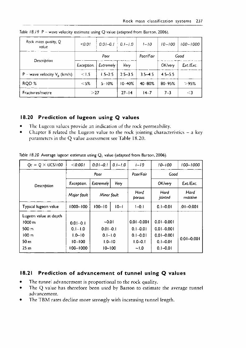
R o ck mass c lass i f ica t ion sys tem s 237
Table 18.19 P - wave velocity estimate using Q value (adapted from Barton, 2006).
Rock mass quality, Q value <0.01 0.01-0.1 O .I- I .O 1-10 10-100 1 0 0 -1 0 0 0
DescriptionPoor Poor/Fair Good
Exception. Extremely Very OK/very ExtJExc .
P - wave velocity Vp (km/s) <1.5 1.5-2.5 2.5-3.5 3.5—4.5 4.5-5.5
RQ D % <5% 5-10% 10-40% 40-80% 80-95% >95%
Fractures/metre >27 27-14 14-7 7-3 <3
18.20 Prediction of lugeon using Q values• The Lugeon values provide an indication of the rock permeability.• Chapter 8 related the Lugeon value to the rock jointing characteristics - a key
parameters in the Q value assessment see Table 18.20.
Table 18.20 Average lugeon estimate using Q c value (adapted from Barton, 2006).
Qc = Q x UCS/100 < 0.001 0 .01-0 .1 O .I- I .O 1-10 10-100 100-1000
Description
Poor Poor/Fair Good
Exception. Extremely Very OK/very Ext/Exc .
M ajor fault Minor fault Hardporous
Hardjointed
Hardmassive
Typical lugeon value 1000-100 100-10 10-1 1-0. 0.1-0.01 .01-0.001
Lugeon value at depth1000 m500 m100 m50 m25 m
0.01-0.1 O .I-I.O 1.0-10 10-100
100-1000
-0.01 0.01 -0.1 O.I-I.O 1.0-10 10-100
0.01-0.001 0.1-0.01 0.1-0.01 1.0-0.1 -1 .0
0.01-0.001 0.01-0.001 0.01-0.001
0.1-0.01 0.1-0.01
0.01-0.001
18.21 Predict ion of a d van cem en t of tunnel using Q values• The tunnel advancement is proportional to the rock quality.• The Q value has therefore been used by Barton to estimate the average tunnel
advancement.• The T B M rates decline more strongly with increasing tunnel length.
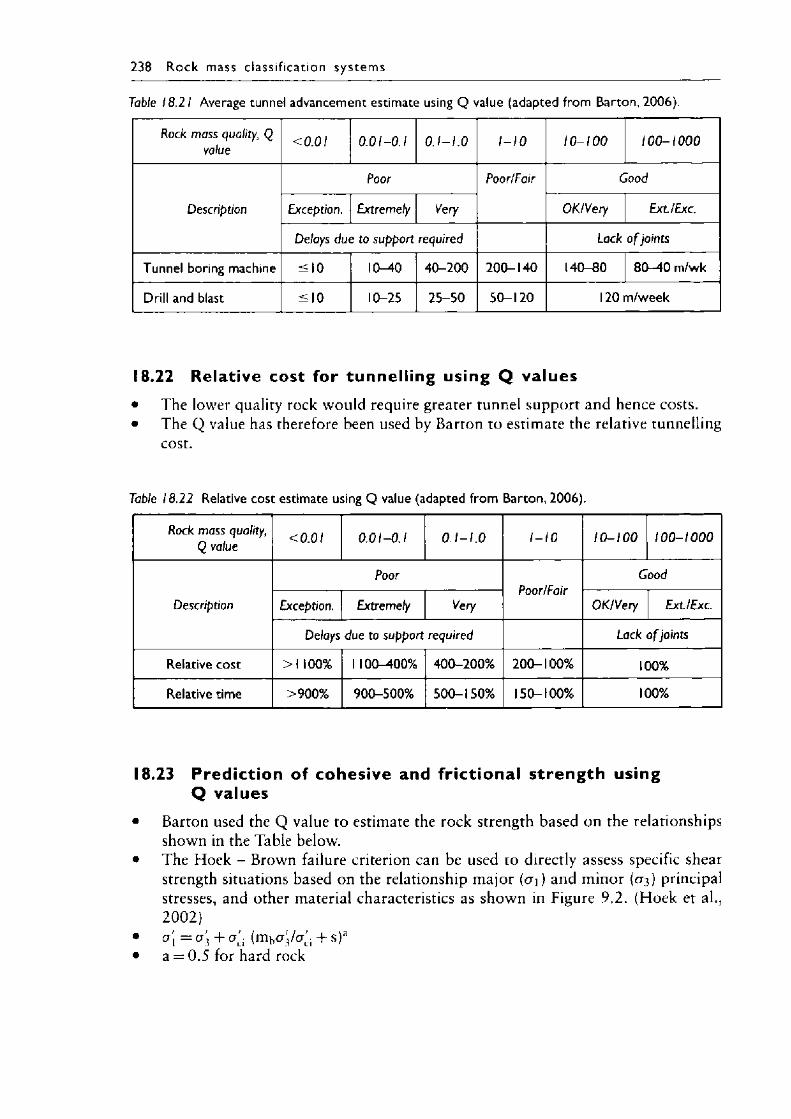
238 R o c k mass c la ss i f ica t ion sy s te m s
Table 18.2 I Average tunnel advancement estimate using Q value (adapted from Barton, 2006).
Rock mass quality, Q value < 0.01 0 .01-0.1 O .I- I .O 1-10 10-100 100-1000
Description
Poor Poor/Fair Good
Exception. Extremely Very OK/Very Ext/Exc.
Delays due to support required Lack o f joints
Tunnel boring machine <10 10-40 40-200 200-140 140-80 80—40 m/wk
Drill and blast <10 10-25 25-50 50-120 120 m/week
18.22 Relative cost for tunnelling using Q values• The lower quality rock would require greater tunnel support and hence costs.• The Q value has therefore been used by Barton to estimate the relative tunnelling
cost.
Table 18.22 Relative cost estimate using Q value (adapted from Barton, 2006).
Rock mass quality, Q value < 0.01 0 .01-0.1 O .I- I .O 1-10 10-100 100-1000
Description
PoorPoor/Fair
Good
Exception. Extremely Very OK/Very Ext/Exc .
Delays due to support required Lack o f joints
Relative cost >1 100% 1 100-^00% 400-200% 200-100% 100%
Relative time >900% 900-500% 500-150% 150-100% 100%
18.23 Prediction of cohesive and fr ict ional strength using Q values
• Barton used the Q value to estimate the rock strength based on the relationships shown in the Table below.
• The Hoek - Brown failure criterion can be used to directly assess specific shear strength situations based on the relationship m ajor (a i) and minor (a^) principal stresses, and other material characteristics as shown in Figure 9 .2 . (Hoek et al., 2002)
• o\ = a ' + a'j (mbcr;/(j' + s)a• a = 0 .5 for hard rock
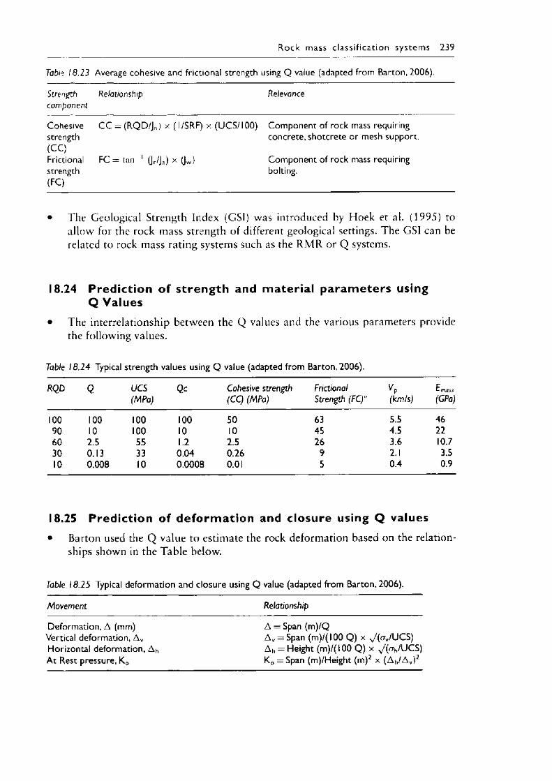
R o ck mass c la ss i f ica t ion sys tem s 239
Table 18.23 Average cohesive and frictional strength using Q value (adapted from Barton, 2006).
Strength Relationship Relevancecomponent
Cohesive C C — (RQD/Jn) x ( l/SRF) x (U C S/100) Component of rock mass requiringstrength concrete, shotcrete or mesh support.(CC)Frictional *XIIULL Component of rock mass requiringstrength bolting.(FC)
• The Geological Strength Index (GSI) was introduced by Hoek et al. (1995) to allow for the rock mass strength of different geological settings. The GSI can be related to rock mass rating systems such as the R M R or Q systems.
18.24 Predict ion of strength and material p aram eters using Q Values
• The interrelationship between the Q values and the various parameters provide the following values.
Table 18.24 Typical strength values using Q value (adapted from Barton, 2006).
RQD Q UCS(MPa)
Qc Cohesive strength (CC) (MPa)
Frictional Strength (FC)°
Vp(km/s)
E-mass(GPa)
100 100 100 100 50 63 5.5 4690 10 100 10 10 45 4.5 2260 2.5 55 1.2 2.5 26 3.6 10.730 0.13 33 0.04 0.26 9 2.1 3.510 0.008 10 0.0008 0.01 5 0.4 0.9
18.25 Predict ion of deform ation and closure using Q values• Barton used the Q value to estimate the rock deformation based on the relation
ships shown in the Table below.
Table 18.25 Typical deformation and closure using Q value (adapted from Barton, 2006).
Movement Relationship
Deformation, A (mm) A = Span (m)/QVertical deformation, A v A v = Span (m)/( 100 Q ) x ^ /(a JU C S )Horizontal deformation, A h A h = Height (m)/( 100 Q ) x ^ (a h/UCS)At Rest pressure, K0 K0 = Span (m)/Height (m)2 x (A h/A v)2
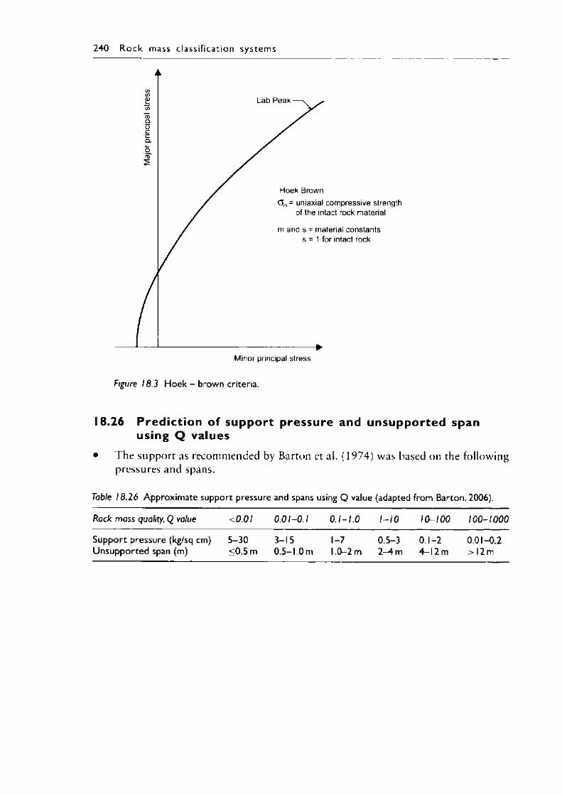
240 R o c k mass c lass i f ica t ion sys tem s
Figure 18.3 Hoek - brown criteria.
18.26 Predict ion of support pressure and unsupported span using Q values
• T he support as recommended by Barton et al. (1974) was based on the following pressures and spans.
Table 18.26 Approximate support pressure and spans using Q value (adapted from Barton, 2006).
Rock mass quality, Q value < 0.01 0.01-0.1 O .I- I .O 1-10 10-100 100-1000
Support pressure (kg/sq cm) Unsupported span (m)
5-30 <0.5 m
3-150.5-1.0 m
1-71.0-2 m
0.5-3 2—4 m
0.1-2 4—12 m
0.01-0.2 > 12 m
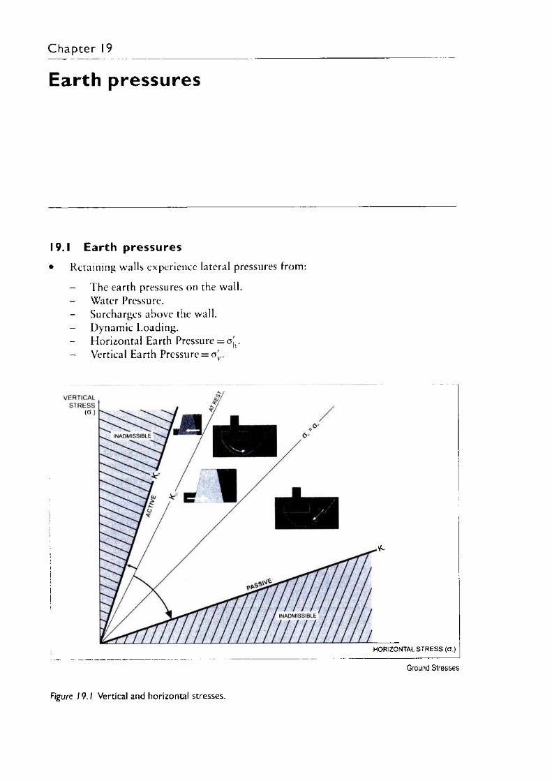
Chapter 19
Earth pressures
19.1 Earth pressures• Retaining walls experience lateral pressures from:
The earth pressures on the wall.- Water Pressure.- Surcharges above the wall.- Dynamic Loading.
Horizontal Earth Pressure = a ! .Vertical Earth Pressure = o'v.
HO RIZO N TAL S T R E S S (a ,)
Ground Stresses
Figure 19 .1 Vertical and horizontal stresses.
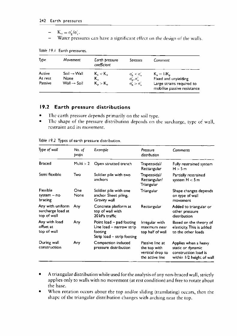
242 E a r th p re ssu re s
- K0 =a'/a;.- Water pressures can have a significant effect on the design of the walls.
Table 19. / Earth pressures.
Type Movement Earth pressure coefficient
Stresses Comment
Active Soil —> Wall Ka < K 0 a h < a v Ka = l/ K pAt rest None Ko a h ’ a v Fixed and unyieldingPassive Wall — Soil Kp > K0 ° h > a v Large strains required to
mobilise passive resistance
19.2 Earth pressure distr ibutions• The earth pressure depends primarily on the soil type.• The shape of the pressure distribution depends on the surcharge, type of wall,
restraint and its movement.
Table 19.2 Types of earth pressure distribution.
Type o f wall No. o f props
Example Pressuredistribution
Comments
Braced Multi > 2 Open strutted trench Trapezoidal/Rectangular
Fully restrained system H > 5 m
Semi flexible Two Soldier pile with two anchors
Trapezoidal/Rectangular/Triangular
Partially restrained system H < 5 m
Flexible system - no bracing
OneNone
Soldier pile with one anchor Sheet piling, Gravity wall
Triangular Shape changes depends on type of wall movement
Any with uniform surcharge load at top of wall
Any Concrete platform at top of wall with 20 kPa traffic
Rectangular Added to triangular or other pressure distribution
Any with load offset at top of wall
Any Point load - pad footing Line load - narrow strip footingStrip load - strip footing
Irregular with maximum near top half of wall
Based on the theory of elasticity. This is added to the other loads
During wall construction
Any Compaction induced pressure distribution
Passive line at the top with vertical drop to the active line
Applies when a heavy static or dynamic construction load is within 1/2 height of wall
• A triangular distribution while used for the analysis of any non-braced wall, strictly applies only to walls with no movement (at rest condition) and free to rotate about the base.
• When rotation occurs about the top and/or sliding (translating) occurs, then the shape of the triangular distribution changes with arching near the top.
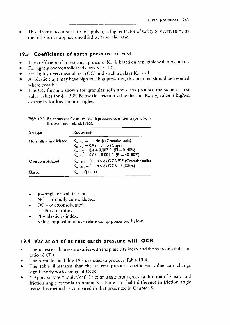
Earth p re s s u re s 243
• This effect is accounted for by applying a higher factor of safety to overturning as the force is not applied one-third up from the base.
19.3 Coeffic ients of earth pressure at rest• The coefficient of at rest earth pressure (K0) is based on negligible wall movement.• For lightly overconsolidated clays K() ~ 1.0.• For highly overconsolidated (OC) and swelling clays K() » 1.• As plastic clays may have high swelling pressures, this material should be avoided
where possible.• The O C formula shown for granular soils and clays produce the same at rest
value values for cj> = 30°. Below this friction value the clay K0 (oc) value is higher,especially for low friction angles.
Tabie 19.3 Relationships for at rest earth pressure coefficients (part from Brooker and Ireland, 1965).
Soil type Relationship
Normally consolidated K0 (NC) = 1 - sin (\> (Granular soils)K0 (N C ) = 0.95 - sin <|> (Clays)K0 (N C) = 0.4 - f 0.007 PI (PI = 0-40%)K0 (n o = 0.64 + 0.001 PI (PI = 40-80%)
Overconsolidated K 0 (O C ) = (1 - sin <|>) O C R sm * (Granular soils) K0 (O C ) = (1 — sin cj)> O C R 1/2 (Clays)
Elastic K„ = v/( 1 - v)
(J) - angle of wall friction.- NC - normally consolidated.- O C - overconsolidated,
v - Poisson ratio.- PI - plasticity index.
Values applied in above relationship presented below.
19.4 Variat ion of at rest earth pressure with O C R• The at-rest earth pressure varies with the plasticity index and the overconsolidation
ratio (OCR).• The formulae in Table 19.3 are used to produce Table 19.4.• The table illustrates that the at rest pressure coefficient value can change
significantly with change of O C R .• * Approximate “ Equivalent” Friction angle from cross calibration of elastic and
friction angle formula to obtain K(). Note the slight difference in friction angle using this method as compared to that presented in Chapter 5.
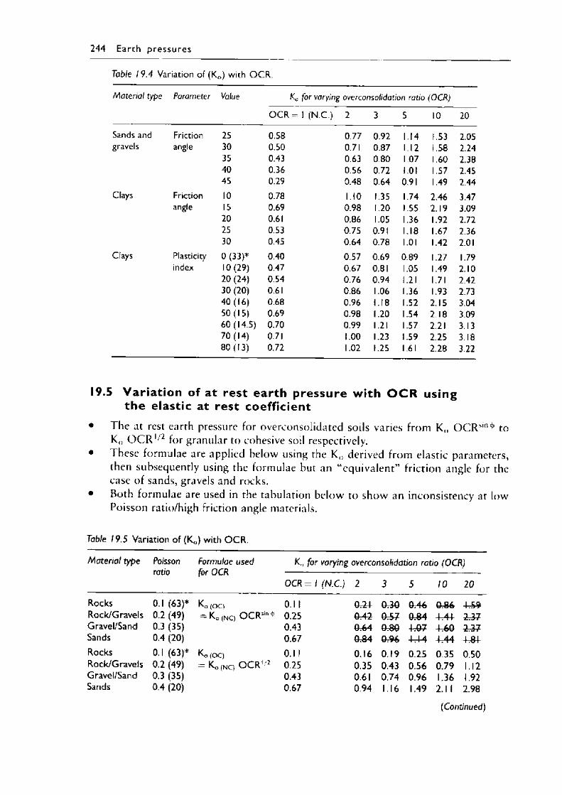
244 E a r th p re ssu re s
Table 19.4 Variation of (K0) with O C R .
Material type Parameter Value K0 for varying overconsolidation ratio (OCR)
O C R = 1 (N.C.) 2 3 5 10 20
Sands and Friction 25 0.58 0.77 0.92 1.14 1.53 2.05gravels angle 30 0.50 0.71 0.87 1.12 1.58 2.24
35 0.43 0.63 0.80 1.07 1.60 2.3840 0.36 0.56 0.72 1.01 1.57 2.4545 0.29 0.48 0.64 0.91 1.49 2.44
Clays Friction 10 0.78 1.10 1.35 1.74 2.46 3.47angle 15 0.69 0.98 1.20 1.55 2.19 3.09
20 0.61 0.86 1.05 1.36 1.92 2.7225 0.53 0.75 0.91 1.18 1.67 2.3630 0.45 0.64 0.78 1.01 1.42 2.01
Clays Plasticity 0(33)* 0.40 0.57 0.69 0.89 1.27 1.79index 10(29) 0.47 0.67 0.81 1.05 1.49 2.10
20 (24) 0.54 0.76 0.94 1.21 1.71 2.4230 (20) 0.61 0.86 1.06 1.36 1.93 2.7340 (16) 0.68 0.96 1.18 1.52 2.15 3.0450(15) 0.69 0.98 1.20 1.54 2.18 3.0960 (14.5) 0.70 0.99 1.21 1.57 2.21 3.1370 (14) 0.71 1.00 1.23 1.59 2.25 3.1880 (13) 0.72 1.02 1.25 1.61 2.28 3.22
19.5 Var iat ion of at rest earth pressure with O C R using the elastic at rest coefficient
• The at rest earth pressure for overconsolidated soils varies from K„ O C R sm<1, to K() O C R 1/2 for granular to cohesive soil respectively.
• These formulae are applied below using the K„ derived from elastic parameters, then subsequently using the formulae but an “equivalent” friction angle for the case o f sands, gravels and rocks.
• Both formulae are used in the tabulation below to show an inconsistency at low Poisson ratio/high friction angle materials.
Table 19.5 Variation of (K0) with O C R .
Material type Poisson Formulae used K,, for varying overconsolidation ratio (OCR)IUUU j u i wv-rv
O C R = 1 ( N . C . ) 2 3 5 10 20
Rocks 0.1 (63)* Ko (O O 0.1 1 054 n inv. Jv &46 o Q£v.OwRock/Gravels 0.2 (49) = K0(NQ O C R sin* 0.25 QA2 0^ 7 n 04V.O T -W 4 2^7Gravel/Sand 0.3 (35) 0.43 Q CAV.V T & WSands 0.4 (20) 0.67 0 QAv.U I 0^ 6 4^14 4r44Rocks 0.1 (63)* Ko (oc) 0.1 1 0.16 0.19 0.25 0.35 0.50Rock/Gravels 0.2 (49) = K0 (NC) O C R 1 2 0.25 0.35 0.43 0.56 0.79 1.12Gravel/Sand 0.3 (35) 0.43 0.61 0.74 0.96 1.36 1.92Sands 0.4 (20) 0.67 0.94 1.16 1.49 2.1 1 2.98
(Continued)
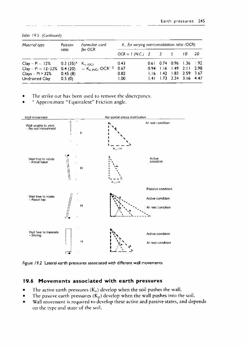
Earth p re s s u re s 245
Table 19.5 (Continued)
Material type Poisson Formulae used K,, for varying overconsolidation ratio (OCR)ratio for u l a
OCR = 1 (N.C.) 2 3 5 10 20
Clay - PI < 12% 0.3 (35)* K 0 (OC) 0.43 0.61 0.74 0.96 1.36 1.92Clay - PI = 12-22% 0.4 (20) = K0 (NC) O C R 1 2 0.67 0.94 1.16 1.49 2.1 1 2.98Clays - PI > 32% 0.45 (8) 0.82 1.16 1.42 1.83 2.59 3.67Undrained Clay 0.5 (0) 1.00 1.41 1.73 2.24 3.16 4.47
• The strike out has been used to remove the discrepancy.• * Approximate ‘■‘Equivalent” Friction angle.
Wall movement Horizontal stress distribution
Wall unable to yield - No wall movement
K: s <
: \I \I ____________ >
K „ y H
At rest condition
Wall free to rotate - About base
Wall free to rotate - About top
» \• > i \ a i \ i \ i ' i '•______:
K , y H
Activecondition
\ I \/\ V ' ‘ v
Passive condition
Active condition
At rest condition
Wall free to translate - Sliding
kActive condition
\ NH y > At rest condition
/ ' s____I ' N
Figure 19.2 Lateral earth pressures associated with different wall movements.
19.6 Movements assoc iated with earth pressures• The active earth pressures (Ka) develop when the soil pushes the wall.• The passive earth pressures (Kp) develop when the wall pushes into the soil.• Wall movement is required to develop these active and passive states, and depends
on the type and state o f the soil.
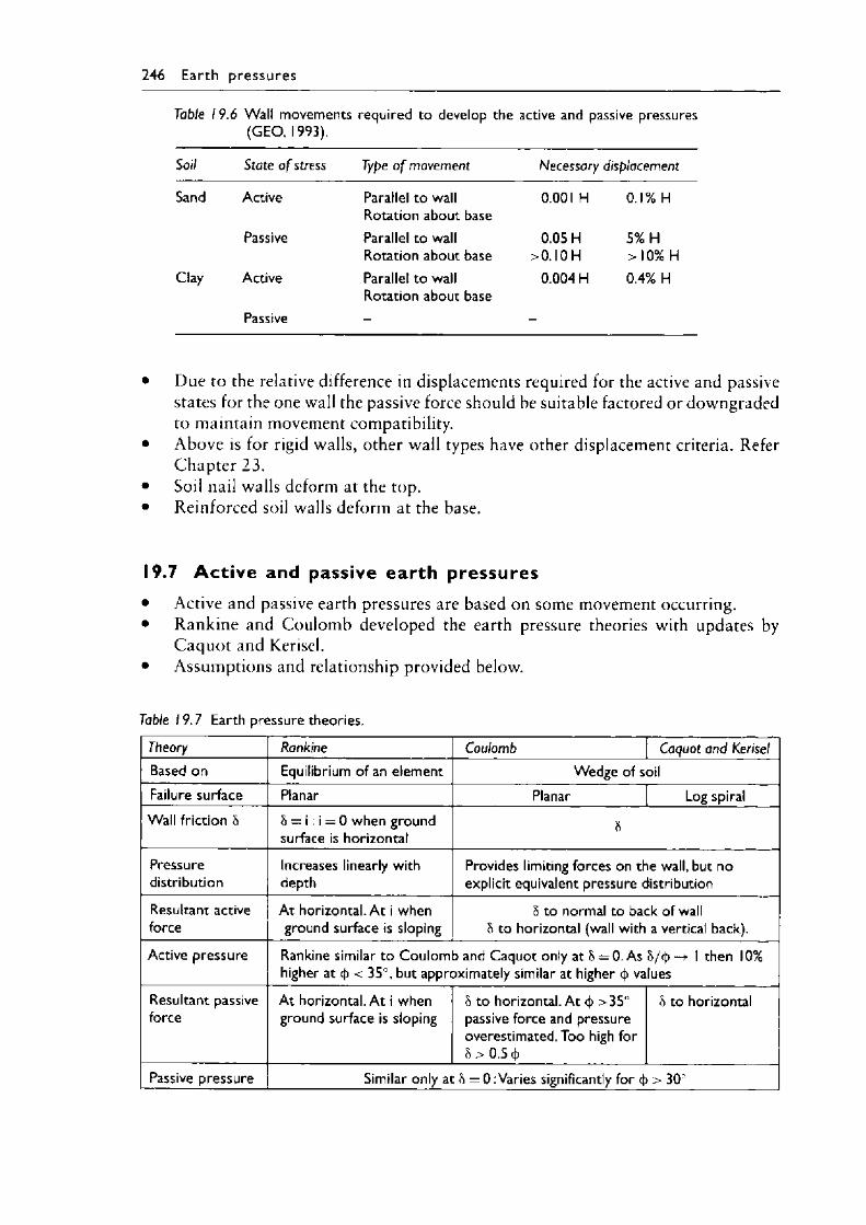
246 E a r th p re ssu re s
Table 19.6 Wall movements required to develop the active and passive pressures (GEO, 1993).
Soil State o f stress Type o f movement Necessary displacement
Sand Active Parallel to wall Rotation about base
0.001 H 0.1% H
Passive Parallel to wall Rotation about base
0.05 H >0.10 H
5% H >10% H
Clay Active Parallel to wall Rotation about base
0.004 H 0.4% H
Passive - -
• Due to the relative difference in displacements required for the active and passive states for the one wall the passive force should he suitable factored or downgraded to maintain movement compatibility.
• Above is for rigid walls, other wall types have other displacement criteria. Refer Chapter 23.
• Soil nail walls deform at the top.• Reinforced soil walls deform at the base.
19.7 A ct ive and passive earth pressures• Active and passive earth pressures are based on some movement occurring.• Rankine and Coulomb developed the earth pressure theories with updates by
Caquot and Kerisel.• Assumptions and relationship provided below.
Table 19.7 Earth pressure theories.
Theory Rankine Coulomb Caquot and KeriselBased on Equilibrium of an element Wedge of soilFailure surface Planar Planar Log spiralWall friction 8 & = j : i = 0 when ground
surface is horizontal8
Pressuredistribution
Increases linearly with depth
Provides limiting forces on the wall, but no explicit equivalent pressure distribution
Resultant active force
At horizontal. At i when ground surface is sloping
h to normal to back of wall h to horizontal (wall with a vertical back).
Active pressure Rankine similar to Coulomb and Caquot only at h = 0. As &/<j) —> 1 then 10% higher at < 35°, but approximately similar at higher (j) values
Resultant passive force
At horizontal. At i when ground surface is sloping
h to horizontal. At 4> >35° passive force and pressure overestimated. Too high for8 > 0.5 cj>
5 to horizontal
Passive pressure Similar only at h = 0 :Varies significantly for 4> > 30
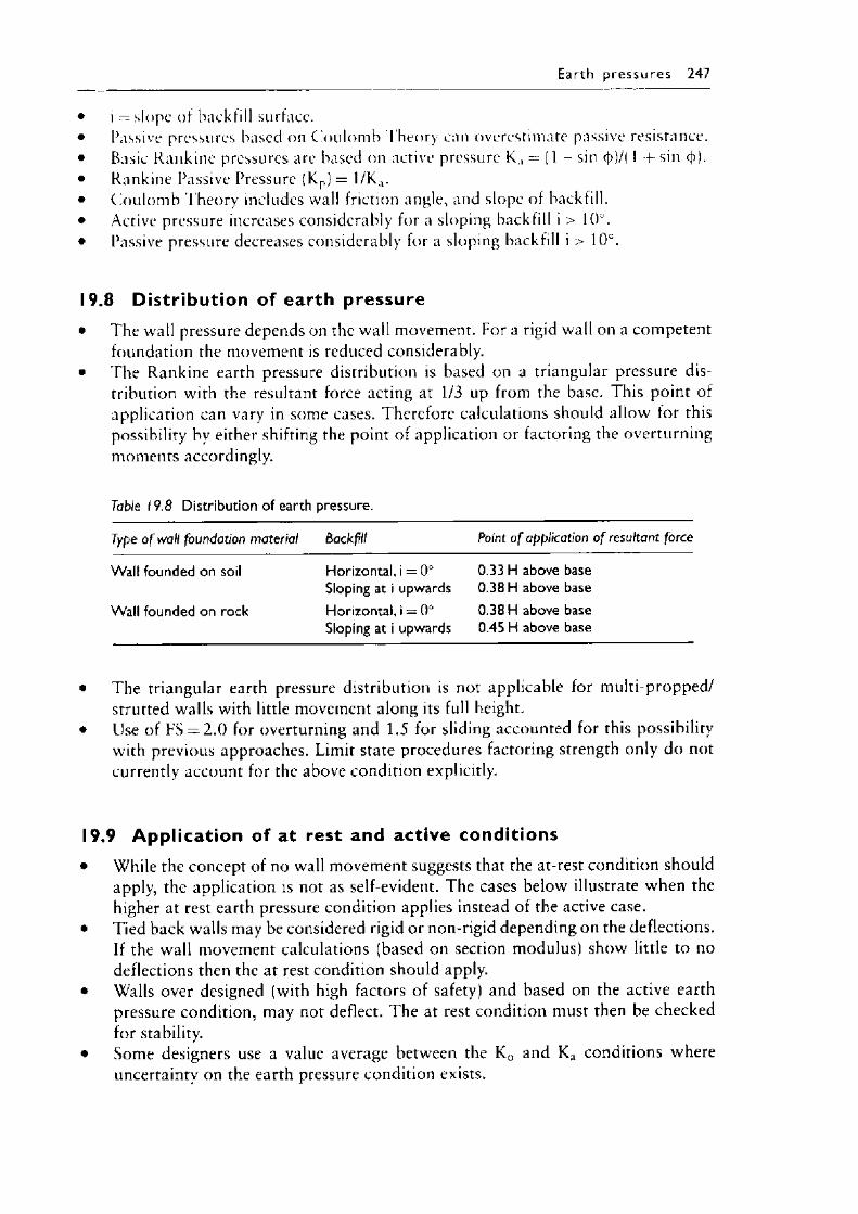
Ear th p re s s u re s 247
• i = slope of backfill surface.• Passive pressures based on Coulomb Theory can overestimate passive resistance.• Basic Rankine pressures arc based on active pressure K., = (1 - sin ()>)/( 1 sin <)>).• Rankine Passive Pressure (Kp) = 1/Kn.• (Coulomb Theory includes wall friction angle, and slope of backfill.• Active pressure increases considerably for a sloping backfill i > 10°.• Passive pressure decreases considerably for a sloping backfill i > 10°.
19.8 Distribution of earth pressure• The wall pressure depends on the wall movement. For a rigid wall on a competent
foundation the movement is reduced considerably.• The Rankine earth pressure distribution is based on a triangular pressure dis
tribution with the resultant force acting at 1/3 up from the base. This point of application can vary in some cases. Therefore calculations should allow for this possibility by either shifting the point of application or factoring the overturning moments accordingly.
Table 19.8 Distribution of earth pressure.
Type o f wall foundation material Backfill Point o f application o f resultant force
Wall founded on soil Horizontal, i = 0° 0.33 H above baseSloping at i upwards 0.38 H above base
Wall founded on rock Horizontal, i = 0° 0.38 H above baseSloping at i upwards 0.45 H above base
• The triangular earth pressure distribution is not applicable for multi-propped/ strutted walls with little movement along its full height.
• Use of FS = 2 .0 for overturning and 1.5 for sliding accounted for this possibility with previous approaches. Limit state procedures factoring strength only do not currently account for the above condition explicitly.
19.9 Application of at rest and active conditions• While the concept of no wall movement suggests that the at-rest condition should
apply, the application is not as self-evident. The cases below illustrate when the higher at rest earth pressure condition applies instead of the active case.
• Tied back walls may be considered rigid or non-rigid depending on the deflections. If the wall movement calculations (based on section modulus) show little to no deflections then the at rest condition should apply.
• Walls over designed (with high factors of safety) and based on the active earth pressure condition, may not deflect. The at rest condition must then be checked for stability.
• Some designers use a value average between the K() and Ka conditions where uncertainty on the earth pressure condition exists.
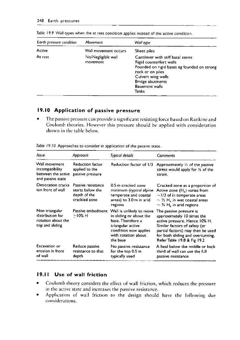
248 Earth p re ssu res
Table 19.9 Wall types when the at rest condition applies instead of the active condition.
Earth pressure condition Movement Wall type
Active Wall movement occurs Sheet pilesAt rest No/Negligible wall Cantilever with stiff basal stems
movement Rigid counterfort wallsFounded on rigid bases eg founded on strongrock or on pilesCulvert wing wallsBridge abutmentsBasement wallsTanks
19.10 Application of passive p ressure• The passive pressure can provide a significant resisting force based on Rankine and
Coulomb theories. However this pressure should be applied with consideration shown in the table below.
Table 19.10 Approaches to consider in application of the passive state.
Issue Approach Typical details Comments
Wall movement Reduction factor Reduction factor of 1 /3 Approximately Vi of the passiveincompatibility applied to the stress would apply for 'A of thebetween the active passive pressure strain.and passive stateDesiccation cracks Passive resistance 0.5 m cracked zone Cracked zone as a proportion ofion front of wall starts below the minimum (typical alpine Active zone (Ha) varies from
depth of the temperate and coastal ~ l/3 of in temperate areascrackled zone areas) to 3.0 m in arid ~ Zi Ha in wet coastal areas
regions ~ 3A Ha in arid regionsNon triangular Passive embedment Wall is unlikely to move The passive pressure isdistribution for >10% H in sliding or about the approximately 10 times therotation about the base. Therefore a active pressure. Hence 10% H.top and sliding triangular active Similar factors of safety (or
condition now applies partial factors) may then be usedwith rotation about for both sliding and overturning.the base Refer Table 19.8 & Fig 19.2
Excavation or Reduce passive No passive resistance A heel below the middle or backerosion in front resistance to that for the top 0.5 m third of wall can use the fullof wall depth typically used passive resistance
19.11 U se of wall fr iction• Coulomb theory considers the effect o f wall friction, which reduces the pressure
in the active state and increases the passive resistance.• Application of wall friction to the design should have the following due
considerations.
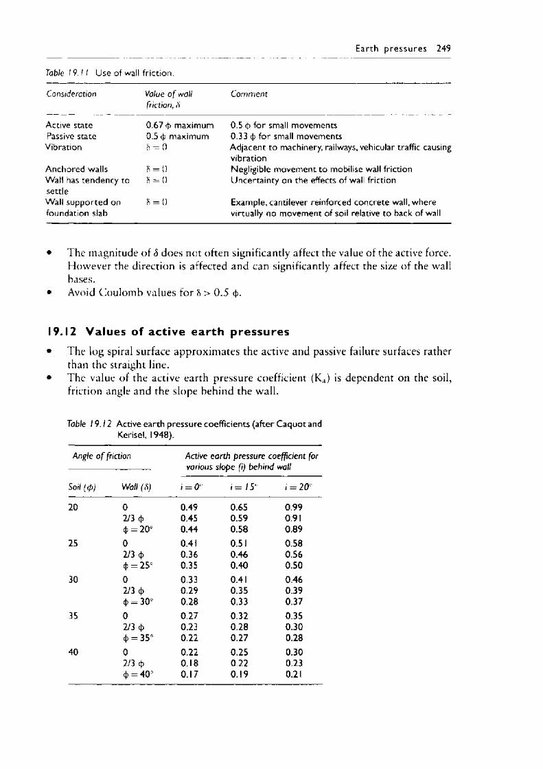
E ar th p re ssu re s 249
Table 19.11 Use of wall friction.
Consideration Value o f wall friction, 6
Comment
Active state 0.67 4> maximum 0.5 cj> for small movementsPassive state 0.5 (J) maximum 0.33 (}) for small movementsVibration 8 = 0 Adjacent to machinery, railways, vehicular traffic causing
vibrationAnchored walls 8 = 0 Negligible movement to mobilise wall frictionWall has tendency to settle
8 = 0 Uncertainty on the effects of wall friction
Wall supported on foundation slab
8 = 0 Example, cantilever reinforced concrete wall, where virtually no movement of soil relative to back of wall
• The magnitude of S does not often significantly affect the value of the active force. However the direction is affected and can significantly affect the size of the wallbases.
• Avoid Coulomb values for 8 > 0 .5 4>-
19.12 Values of act ive earth pressures• The log spiral surface approxim ates the active and passive failure surfaces rather
than the straight line.• The value of the active earth pressure coefficient (Ka) is dependent on the soil,
friction angle and the slope behind the wall.
Table 19.12 Active earth pressure coefficients (after Caquot and Kerisel, 1948).
Angle o f friction Active earth pressure coefficient for various slope (i) behind wall
Soil ( (f)) Wall (S) i = 0 i = 15° / = 20
20 0 0.49 0.65 0.992/3 4> 0.45 0.59 0.91(j) = 20‘ 0.44 0.58 0.89
25 0 0.41 0.51 0.582/3 4> 0.36 0.46 0.564> = 25 0.35 0.40 0.50
30 0 0.33 0.41 0.462/3 4> 0.29 0.35 0.394) = 30° 0.28 0.33 0.37
35 0 0.27 0.32 0.352/3 4> 0.23 0.28 0.304> = 35° 0.22 0.27 0.28
40 0 0.22 0.25 0.302/3 4> 0.18 0.22 0.234> = 40 0.17 0.19 0.21
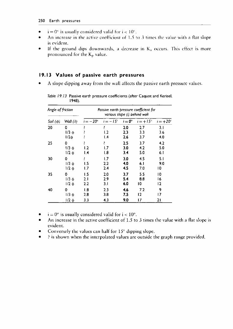
250 Earth p ressures
• i = 0° is usually considered valid for i < 10°.• An increase in the active coefficient of 1.5 to 3 times the value with a flat slope
is evident.• If the ground dips downwards, a decrease in K;1 occurs. This effect is more
pronounced for the Kp value.
19.13 Values of passive earth pressures• A slope dipping away from the wall affects the passive earth pressure values.
Table 19.13 Passive earth pressure coefficients (after Caquot and Kerisel, 1948).
Angle o f friction Passive earth pressure coefficient for various slope (i) behind wall
Soil ((p) Wall (8) i = —20° i = —15° i = 0° j = + / 5° i = +2020 0 ? ? 2.0 2.7 3.1
1/3 4) ? 1.2 2.3 3.3 3.6l/2(}) ? 1.4 2.6 3.7 4.0
25 0 ? ? 2.5 3.7 4.21/3 4> 1.2 1.7 3.0 4.2 5.01/2 (J) 1.4 1.8 3.4 5.0 6.1
30 0 ? 1.7 3.0 4.5 5.11/3 4> 1.5 2.2 4.0 6.1 9.01/2 4) 1.7 2.4 4.5 7.0 10
35 0 1.5 2.0 3.7 5.5 101/3 4> 2.1 2.9 5.4 8.8 161/2 4) 2.2 3.1 6.0 10 12
40 0 1.8 2.3 4.6 7.2 91/3 4) 2.8 3.8 7.5 12 171/2 4) 3.3 4.3 9.0 17 21
• i = 0° is usually considered valid for i < 10°.• An increase in the active coefficient of 1.5 to 3 times the value with a flat slope is
evident.• Conversely the values can half for 15° dipping slope.• ? is shown when the interpolated values are outside the graph range provided.
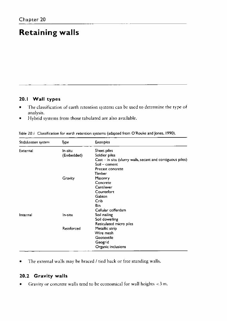
Chapter 20
Retaining walls
20.1 W al l types• The classification of earth retention systems can be used to determine the type of
analysis.• Hybrid systems from those tabulated are also available.
Table 20.1 Classification for earth retention systems (adapted from O ’Rouke and Jones, 1990).
Stabilization system Type Examples
External In-situ Sheet piles(Embedded) Soldier piles
Cast - in situ (slurry walls, secant and contiguous piles)Soil - cementPrecast concreteTimber
Gravity MasonryConcreteCantileverCountefortGabionCribBinCellular cofferdam
Internal In-situ Soil nailingSoil dowellingReticulated micro piles
Reinforced Metallic stripW ire meshGeotextileGeogridOrganic inclusions
• The external walls may be braced / tied back or free standing walls.
20.2 G rav ity walls• Gravity or concrete walls tend to be economical for wall heights < 3 m.
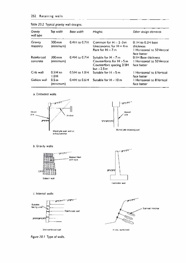
252 Reta in ing walls
Table 20.2 Typical gravity wall designs.
Gravity wall type
Top width Base width Heights Other design elements
Gravity 300 mm 0.4 H to 0.7 H Common for H = 2-3 m 0.IH to 0.2H basemasonry (minimum) Uneconomic for H = 4 m thickness
Rare for H = 7m 1 Horizontal to 50 Verticalface batter
Reinforced 300 mm 0.4 H to 0.7 H Suitable for H <7 m 0.1 H Base thicknessconcrete (minimum) Counterforts for H >5 m 1 Horizontal to 50 Vertical
Counterfort spacing 2/3H face batterbut >2.5 m
Crib wall 0.5 H to 0.5 H to 1.0 H Suitable for H <5 m 1 Horizontal to 6 Vertical1.0 H face batter
Gabion wall 0.5 m 0.4 H to 0.6 H Suitable for H < 10 m 1 Horizontal to 8 Vertical(minimum) face batter
a. Embeded walls
Bored pile retaining wall
b. Gravity walls
Gabion wall
B asket filled with rock
c. Internal walls
Suitable facing units'
7 7 V F 7 7 7
Reinforced soil
Soil reinforced wall
Figure 2 0 .1 Type of walls.
Soil nail / Anchof
In-situ reinforced
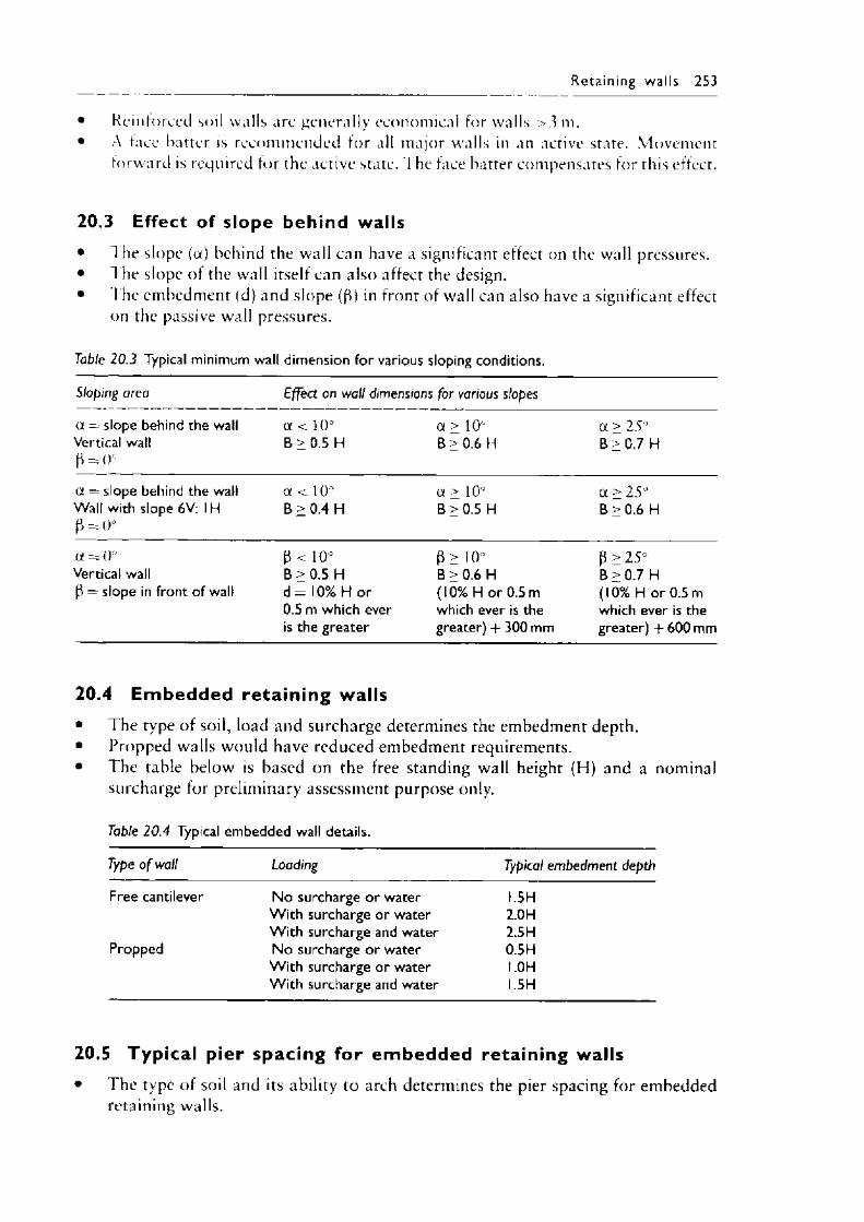
Reta in ing walls 253
• Reinforced soil walls are generally economical for walls >3 m.• A face barter is recommended for all major walls in an active state. Movement
forward is required tor the active state. The face batter compensates for this effect.
20.3 Effect of slope behind walls• I he slope (a) behind the wall can have a significant effect on the wall pressures.• I he slope of the wall itself can also affect the design.• 1 he embedment (d) and slope (P) in front of wall can also have a significant effect
on the passive wall pressures.
Table 20.3 Typical minimum wall dimension for various sloping conditions.
Sloping area Effect on wall dimensions for various slopes
a = slope behind the wall Vertical wall( j= o °
a < 10° B > 0.5 H
a > 10°B > 0.6 H
a > 25°B > 0.7 H
a = slope behind the wall a < 10° a > 10° a > 25°Wall with slope 6V: IH B > 0.4 H B > 0.5 H B > 0.6 HP = 0°
a = 0° p < 10° p> 10° P > 25°Vertical wall B > 0.5 H B > 0.6 H B > 0.7 HP = slope in front of wall d = 10% H or (10% H or 0.5 m (10% H or 0.5 m
0.5 m which ever which ever is the which ever is theis the greater greater) -f 300 mm greater) + 600 mm
20.4 Em bedded retaining walls• The type of soil, load and surcharge determines the embedment depth.• Propped walls would have reduced embedment requirements.• The table below is based on the free standing wall height (H) and a nominal
surcharge for preliminary assessment purpose only.
Table 20.4 Typical embedded wall details.
Type o f wall Loading Typical embedment depth
Free cantilever No surcharge or water I.5HW ith surcharge or water 2.0HW ith surcharge and water 2.5H
Propped No surcharge or water 0.5HW ith surcharge or water 1 .OHW ith surcharge and water I.5H
20.5 Typical pier spacing for embedded retaining walls• The type of soil and its ability to arch determines the pier spacing for embedded
retaining walls.
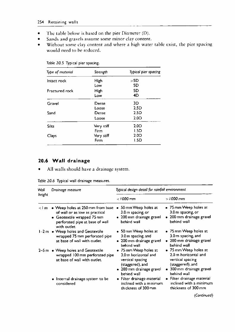
254 R e ta in in g w a l ls
• The table below is based on the pier Diameter (D).• Sands and gravels assume some minor clay content.• W ithout some clay content and where a high water table exist, the pier spacing
would need to be reduced.
Table 20.5 Typical pier spacing.
Type o f material Strength Typical pier spacing
Intact rock High >5DLow 5D
Fractured rock High 5DLow 4D
Gravel Dense 3DLoose 2.5D
Sand Dense 2.5DLoose 2.0D
Silts Very stiff 2.0DFirm I.5D
Clays Very stiff 2.0DFirm I.5D
20.6 W a l l drainage• All walls should have a drainage system.
Table 20.6 Typical wall drainage measures.
Wall Drainage measure height
Typical design detail for rainfall environment
1000 mm 1000 mm
< I m • Weep holes at 250 mm from base of wall or as low as practical
• Geotextile wrapped 75 mm perforated pipe at base of wall with outlet.
1-2 m • Weep holes and Geotextilewrapped 75 mm perforated pipe at base of wall with outlet.
2-5 m • Weep holes and Geotextilewrapped 100 mm perforated pipe at base of wall with outlet.
• Internal drainage system to be considered
50 mm Weep holes at3.0 m spacing, or200 mm drainage gravel behind wall
50 mm Weep holes at3.0 m spacing, and200 mm drainage gravelbehind wall75 mm Weep holes at3.0 m horizontal and vertical spacing (staggered), and200 mm drainage gravel behind wallFilter drainage material inclined with a minimum thickness of 300 mm
75 mm Weep holes at3.0 m spacing, or200 mm drainage gravel behind wall
75 mm Weep holes at3.0 m spacing, and200 mm drainage gravelbehind wall75 mm Weep holes at2.0 m horizontal and vertical spacing (staggered), and300 mm drainage gravel behind wallFilter drainage material inclined with a minimum thickness of 300 mm
(Continued)
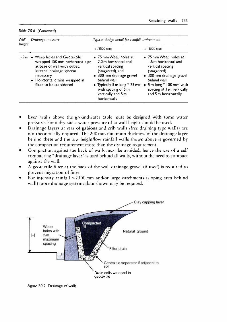
Reta in ing w a l ls 255
Table 20.6 (Continued)
Wallheight
Drainage measure Typical design detail for rainfall environment
< / 000 mm > 1000 mm
>5 m • Weep holes and Geotextile • 75 mm Weep holes at • 75 mm Weep holes atwrapped 150 mm perforated pipe 2.0 m horizontal and 1.5 m horizontal andat base of wall with outlet. vertical spacing vertical spacingInternal drainage system (staggered), and (staggered)necessary • 300 mm drainage gravel • 300 mm drainage gravel
• Horizontal drains wrapped in behind wall behind wallfilter to be considered • Typically 5 m long * 75 mm • 5m long * 100 mm with
with spacing of 5 m spacing of 3 m verticallyvertically and 5 m and 5 m horizontallyhorizontally
• Even walls above the groundwater table must be designed with some water pressure. For a dry site a water pressure of !4 wall height should be used.
• Drainage layers at rear of gabions and crib walls (free draining type walls) are not theoretically required. The 2 0 0 mm minimum thickness of the drainage layer behind these and the low height/low rainfall walls shown above is governed by the compaction requirement more than the drainage requirement.
• Com paction against the back of walls must be avoided, hence the use of a self compacting “drainage layer'’ is used behind all walls, without the need to com pact against the wall.
• A geotextile filter at the back of the wall drainage gravel (if used) is required to prevent migration o f fines.
• For intensity rainfall > 2 5 0 0 mm and/or large catchments (sloping area behind wall) more drainage systems than shown may be required.
Drain coils wrapped in geotextile
Figure 20.2 Drainage of walls.
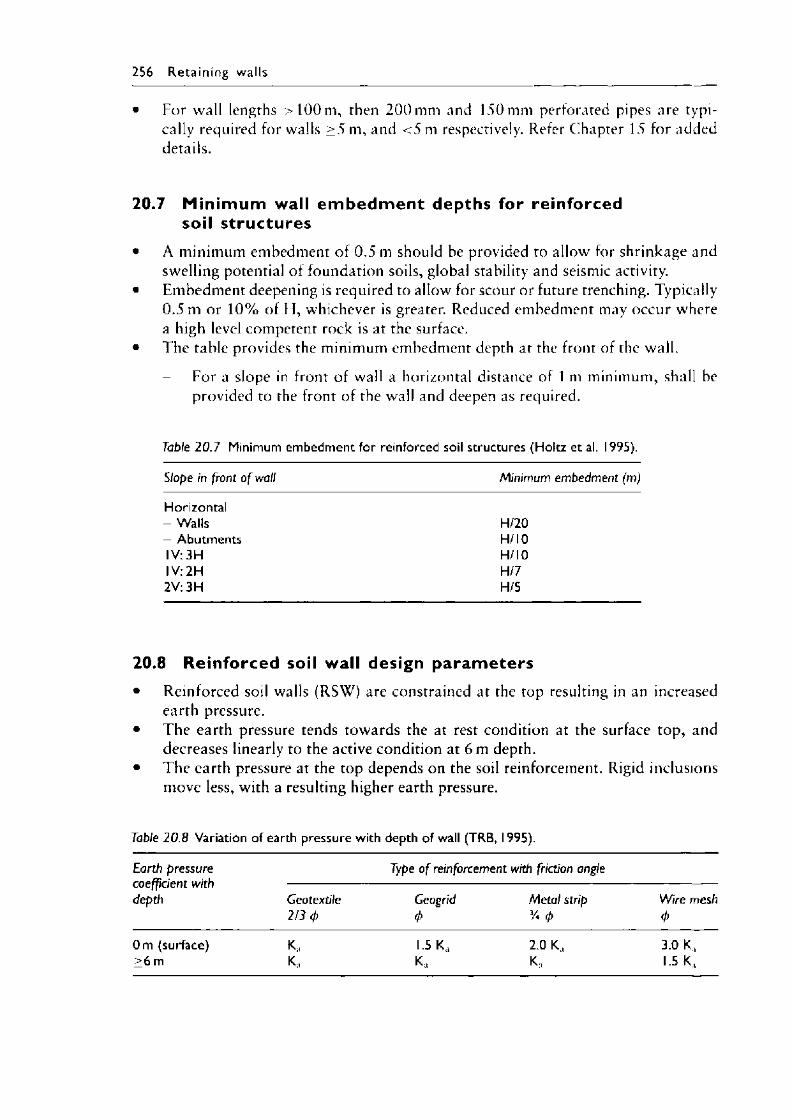
256 R e ta in ing walls
• For wall lengths > 1 0 0 m , then 2 0 0 mm and 150 mm perforated pipes are typically required for walls > 5 m, and < 5 m respectively. Refer Chapter 15 for added details.
20.7 Minimum wall em b ed m ent depths for reinforced soil structures
• A minimum embedment o f 0 .5 m should be provided to allow for shrinkage and swelling potential o f foundation soils, global stability and seismic activity.
• F'mbedment deepening is required to allow for scour or future trenching. Typically 0 .5 m or 1 0 % of H, whichever is greater. Reduced embedment may occur where a high level competent rock is at the surface.
• The table provides the minimum embedment depth at the front of the wall.
- For a slope in front o f wall a horizontal distance of 1 m minimum, shall be provided to the front o f the wall and deepen as required.
Table 20.7 Minimum embedment for reinforced soil structures (Holtz et al. 1995).
Slope in front o f wall Minimum embedment (m)
Horizontal- Walls H/20- Abutments H/10IV: 3H H/10IV: 2H H/72V:3H H/5
20.8 Reinforced soil wall design param eters• Reinforced soil walls (RSW ) are constrained at the top resulting in an increased
earth pressure.• The earth pressure tends towards the at rest condition at the surface top, and
decreases linearly to the active condition at 6 m depth.• The earth pressure at the top depends on the soil reinforcement. Rigid inclusions
move less, with a resulting higher earth pressure.
Table 20.8 Variation of earth pressure with depth of wall (TRB, 1995).
Earth pressure coefficient with depth
Type o f reinforcement with friction angle
Ceotextile213 (p
Geogrid0
Metal strip3/< (p
W ire mesh<t>
0 m (surface) K a 1.5 K, 2.0 K, 3.0 K,> 6 m K , Ka Ka 1.5 K,
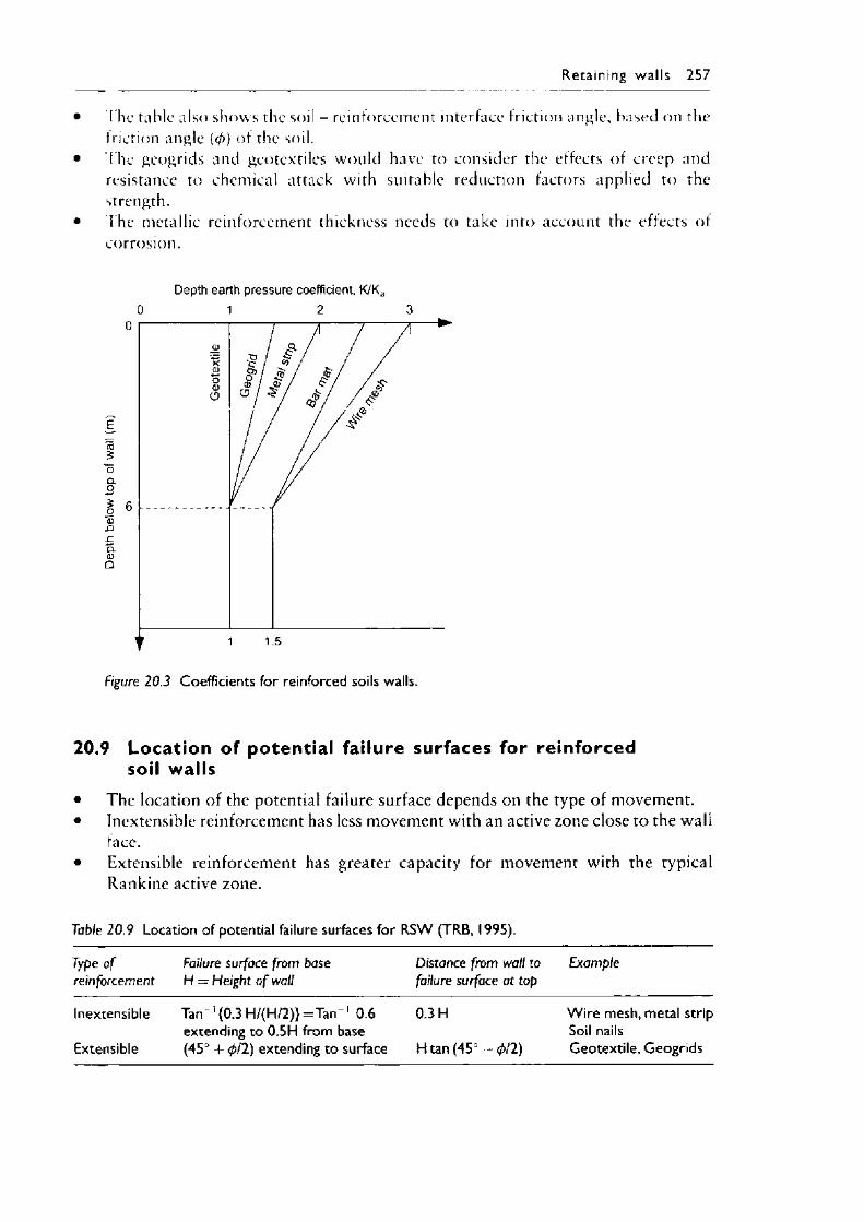
Reta in ing w a l ls 257
• I lie table also shows the soil - reinforcement interface friction angle, based on the friction angle (0) of the soil.
• The geogrids and geotextiles would have to consider the effects of creep and resistance to chemical attack with suitable reduction factors applied to the strength.
• The metallic reinforcement thickness needs to take into account the effects of corrosion.
Depth earth pressure coefficient, K/Ka
Figure 20.3 Coefficients for reinforced soils walls.
20.9 Location of potential failure surfaces for reinforced soil walls
• The location of the potential failure surface depends on the type of movement.• Inextensible reinforcement has less movement with an active zone close to the wall
face.• Extensible reinforcement has greater capacity for movement with the typical
Rankine active zone.
Table 20.9 Location of potential failure surfaces for RSW (TRB, 1995).
Type o f Failure surface from base Distance from wall to Examplereinforcement H = Height o f wall failure surface at top
Inextensible Tan 1 {0.3 H/(H/2)} =Tan 1 0.6 0.3 H W ire mesh, metal stripextending to 0.5H from base Soil nails
Extensible (45° + 0/2) extending to surface H tan (45° — (p/2) Geotextile, Geogrids
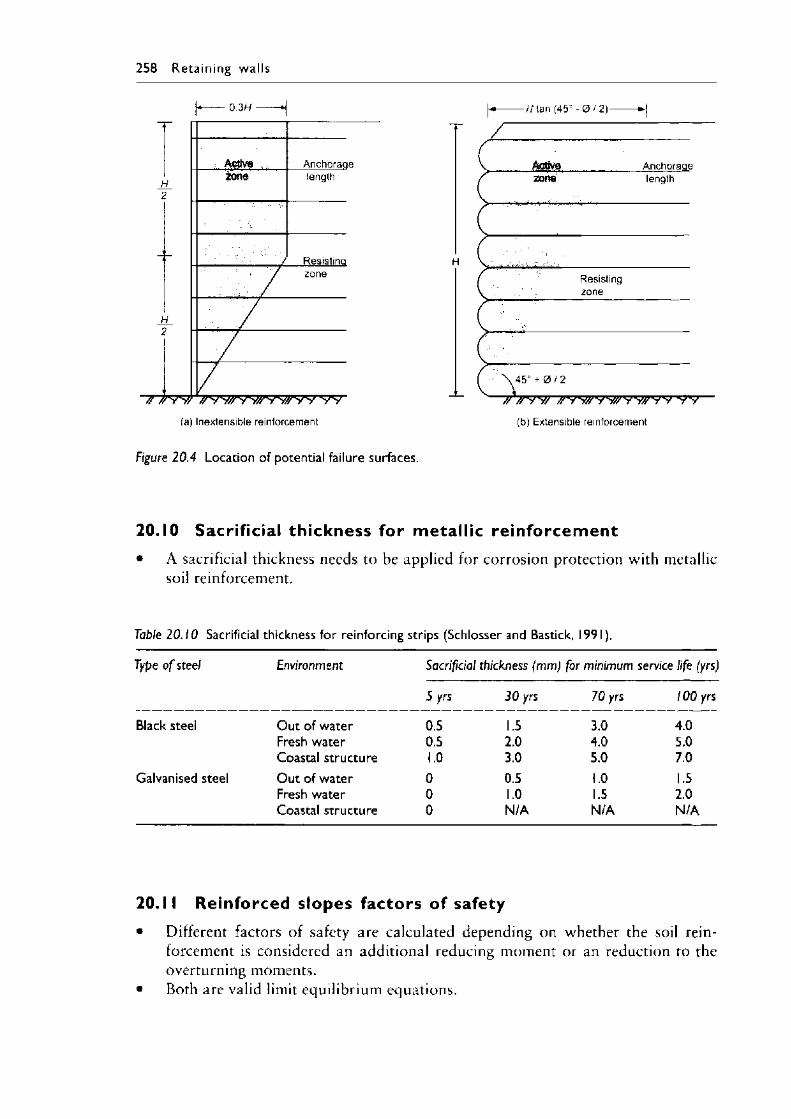
258 Reta in ing w a l ls
0.3H ------ *| -//tan (45° - 0 / 2 )
Figure 20.4 Location of potential failure surfaces.
20.10 Sacrif icial thickness for metallic reinforcement• A sacrificial thickness needs to be applied for corrosion protection with metallic
soil reinforcement.
Table 20.10 Sacrificial thickness for reinforcing strips (Schlosser and Bastick, 1991).
Type o f steel Environment Sacrificial thickness (mm) for minimum service life (yrs)
5 yrs 30 yrs 10 yrs 100 yrs
Black steel Out of water 0.5 1.5 3.0 4.0Fresh water 0.5 2.0 4.0 5.0Coastal structure 1.0 3.0 5.0 7.0
Galvanised steel Out of water 0 0.5 1.0 1.5Fresh water 0 1.0 1.5 2.0Coastal structure 0 N/A N/A N/A
20.11 Reinforced slopes factors of safety• Different factors o f safety are calculated depending on whether the soil rein
forcement is considered an additional reducing moment or an reduction to the overturning moments.
• Both are valid limit equilibrium equations.
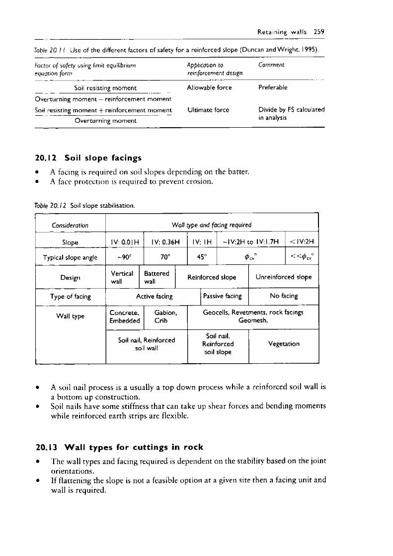
Reta in ing w a l ls 259
Table 2 0 .1 I Use of the different factors of safety for a reinforced slope (Duncan and Wright, 1995).
Factor o f safety using limit equilibrium Application to Commentequation form reinforcement design
Soil resisting moment Allowable force PreferableOverturning moment - reinforcement momentSoil resisting moment 4- reinforcement moment Ultimate force Divide by FS calculated
Overturning moment 'n anatys‘s
20.12 Soil slope facings• A facing is required on soil slopes depending on the batter.• A face protection is required to prevent erosion.
Table 20.12 Soil slope stabilisation.
Consideration Wall type and facing required
Slope IV: 0.01 H IV: 0.36H IV: IH ~IV:2H to IV: 1 7H < 1 V:2H
Typical slope angle -90° 70° 45° 0 C V ° « 0 c v °
Design Verticalwall
Batteredwall Reinforced slope Unreinforced slope
Type of facing Active facing Passive facing No facing
Wall type Concrete,Embedded
Gabion,Crib
Geocells, Revetments, rock facings Geomesh,
Soil nail, Reinforced soil wall
Soil nail, Reinforced soil slope
Vegetation
• A soil nail process is a usually a top down process while a reinforced soil wall is a bottom up construction.
• Soil nails have some stiffness that can take up shear forces and bending moments while reinforced earth strips are flexible.
20.13 W a l l types for cuttings in rock• The wall types and facing required is dependent on the stability based on the joint
orientations.• If flattening the slope is not a feasible option at a given site then a facing unit and
wall is required.
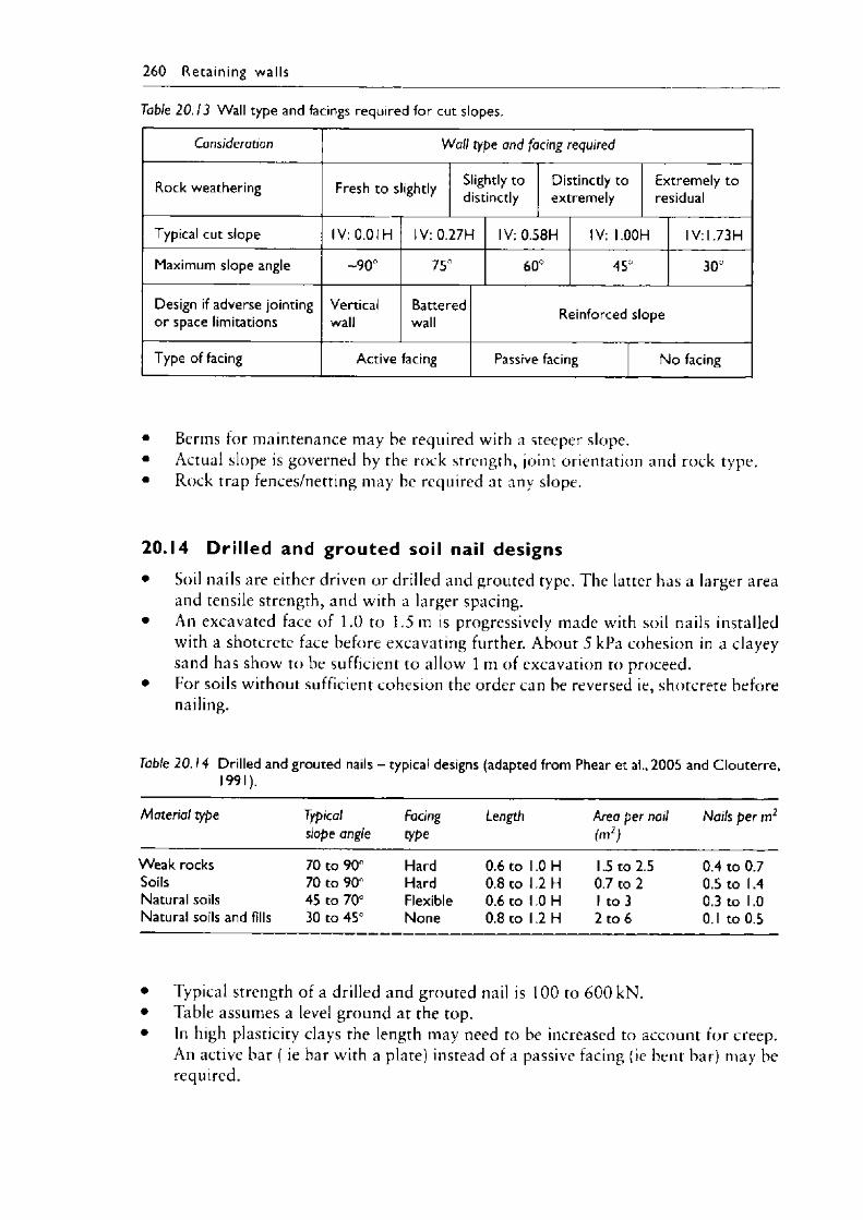
260 Reta in ing walls
Table 20.13 Wall type and facings required for cut slopes.
Consideration Wall type and facing required
Rock weathering Fresh to slightly Slightly to distinctly
Distinctly to extremely
Extremely to residual
Typical cut slope IV: 0.01 H IV: 0.27H IV: 0.58H IV: I.00H IV: 1.73H
Maximum slope angle -90° 75° 60° 45° 30°
Design if adverse jointing or space limitations
Verticalwall
Batteredwall Reinforced slope
Type of facing Active facing Passive facing No facing
• Berms for maintenance may he required with a steeper slope.• Actual slope is governed by the rock strength, joint orientation and rock type.• Rock trap fences/netting may be required at any slope.
20.14 Dril led and grouted soil nail designs• Soil nails are either driven or drilled and grouted type. The latter has a larger area
and tensile strength, and with a larger spacing.• An excavated face of 1.0 to 1.5 m is progressively made w'ith soil nails installed
with a shotcrete face before excavating further. About 5 kPa cohesion in a clayeysand has show to be sufficient to allow 1 m of excavation to proceed.
• For soils without sufficient cohesion the order can be reversed ie, shotcrete before nailing.
Table 2 0 .14 Drilled and grouted nails - typical designs (adapted from Phear et a!., 2005 and Clouterre, 1991).
Material type Typical slope angle
Facingtype
Length Area per nail(m2)
Nails per m2
Weak rocks 70 to 90 Hard 0.6 to 1.0 H 1.5 to 2.5 0.4 to 0.7Soils 70 to 90 Hard 0.8 to 1.2 H 0.7 to 2 0.5 to 1.4Natural soils 45 to 70° Flexible 0.6 to 1.0 H 1 to 3 0.3 to 1.0Natural soils and fills 30 to 45° None 0.8 to 1.2 H 2 to 6 0.1 to 0.5
• Typical strength of a drilled and grouted nail is 100 to 6 0 0 kN.• Table assumes a level ground at the top.• In high plasticity clays the length may need to be increased to account for creep.
An active bar ( ie bar with a plate) instead of a passive facing (ie bent bar) may berequired.
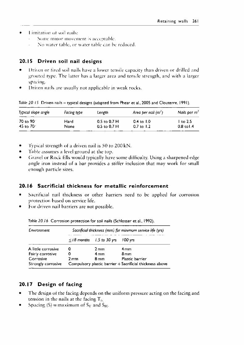
Reta in ing w a l ls 261
• I imitation of soil nails:Some minor movement is acceptable.No water table, or water table can be reduced.
20.15 Driven soil nail designs• Driven or fired soil nails have a lower tensile capacity than driven or drilled and
grouted type. The latter has a larger area and tensile strength, and with a larger spacing.
• Driven nails are usually not applicable in weak rocks.
Table 20.15 Driven nails - typical designs (adapted from Phear et al., 2005 and Clouterre, 1991).
Typical slope angle Facing type Length Area per nail (m2) Nails per m2
70 to 90 Hard 0.5 to 0.7 H 0.4 to 1.0 1 to 2.545 to 70 None 0.5 to 0.7 H 0.7 to 1.2 0.8 to 1.4
• Typical strength of a driven nail is 5 0 to 200 kN.• Table assumes a level ground at the top.• Gravel or Rock fills would typically have some difficulty. Using a sharpened edge
angle iron instead of a bar provides a stiffer inclusion that may work for small enough particle sizes.
20.16 Sacrif ic ial thickness for metallic re inforcement• Sacrificial nail thickness or other barriers need to be applied for corrosion
protection based on service life.• For driven nail barriers are not possible.
Table 20.16 Corrosion protection for soil nails (Schlosser et al., 1992).
Environment Sacrificial thickness (mm) for minimum service life (yrs)
< 18 months 1.5 to 30 yrs 100 yrs
A little corrosive 0 2 mm 4 mmFairly corrosive 0 4 mm 8 mmCorrosive 2 mm 8 mm Plastic barrierStrongly corrosive Compulsory plastic barrier + Sacrificial thickness above
20.17 Design of facing• T he design of the facing depends on the uniform pressure acting on the facing and
tension in the nails at the facing T„• Spacing (S) = maximum of Sy and S h -
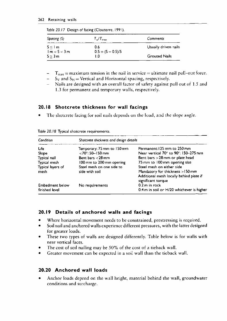
262 Reta in ing walls
Table 2 0 .1 7 Design of facing (Clouterre, 19 9 1).
Spacing (S) Tm ax Comments
S < 1 m 0.6 Usually driven nails1 m < S < 3 m 0.5 + (S - 0.5J/5S > 3 m 1.0 Grouted Nails
- T max = maximum tension in the nail in service = ultimate nail pull-out force.- Sy and Sh = Vertical and Horizontal spacing, respectively.- Nails are designed with an overall factor o f safety against pull out of 1.5 and
1.3 for permanent and temporary walls, respectively.
20.18 Shotcrete thickness for wall facings• The shotcrete facing for soil nails depends on the load, and the slope angle.
Table 20.18 Typical shotcrete requirements.
Condition Shotcrete thickness and design details
Life Slope Typical nail Typical mesh Typical layers of mesh
Embedment below finished level
Temporary: 75 mm to 150 mm <70°: 50-150 mm Bent bars <28 mm 100 mm to 200 mm opening Steel mesh on one side to side with soil
No requirements
Permanent: 125 mm to 250 mm N ear vertical 70° to 90°: 150-275 mm Bent bars >28 mm or plate head 75 mm to 100 mm opening size Steel mesh on either side Mandatory for thickness > 150 mm Additional mesh locally behind plate if significant torque 0.2 m in rock0.4 m in soil or H/20 whichever is higher
20.19 Details of anchored walls and facings• Where horizontal movement needs to be constrained, prestressing is required.• Soil nail and anchored walls experience different pressures, w'ith the latter designed
for greater loads.• These two types of walls are designed differently. Table below is for walls with
near vertical faces.• The cost of soil nailing may be 5 0 % of the cost of a tieback wall.• Greater movement can be expected in a soil wall than the tieback wall.
20.20 Anchored wall loads• Anchor loads depend on the wall height, material behind the wall, groundwater
conditions and surcharge.
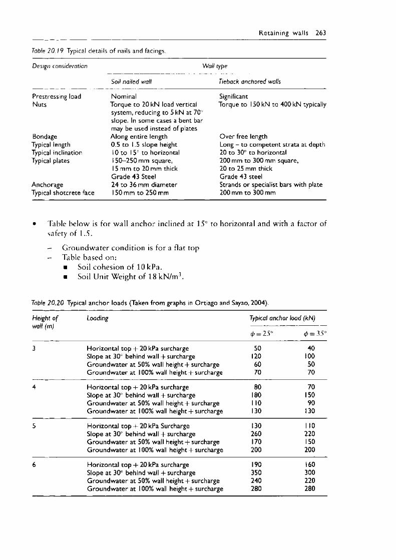
Reta in ing w a l ls 263
Table 20.19 Typical details of nails and facings.
Design consideration Wall type
Soil nailed wall Tieback anchored walls
Prestressing load Nominal SignificantNuts Torque to 20 kN load vertical
system, reducing to 5 kN at 70 slope. In some cases a bent bar may be used instead of plates
Torque to 150 kN to 400 kN typically
Bondage Along entire length Over free lengthTypical length 0.5 to 1.5 slope height Long - to competent strata at depthTypical inclination 10 to 15° to horizontal 20 to 30° to horizontalTypical plates 150-250 mm square, 200 mm to 300 mm square,
1 5 mm to 20 mm thick 20 to 25 mm thickGrade 43 Steel Grade 43 steel
Anchorage 24 to 36 mm diameter Strands or specialist bars with plateTypical shotcrete face 150 mm to 250 mm 200 mm to 300 mm
• Table below is for wall anchor inclined at 15° to horizontal and with a factor of safety of 1.5.
- Groundwater condition is for a flat top- Table based on:
■ Soil cohesion of 10 kPa.■ Soil Unit Weight o f 18 kN/m3.
Table 20.20 Typical anchor loads (Taken from graphs in Ortiago and Sayao, 2004).
Height o f Loading Typical anchor load (kN)wall (m)
0 = 25° -S- II o
3 Horizontal top + 20 kPa surcharge 50 40Slope at 30 behind wall + surcharge 120 100Groundwater at 50% wall height + surcharge 60 50Groundwater at 100% wall height 4- surcharge 70 70
4 Horizontal top + 20 kPa surcharge 80 70Slope at 30° behind wall + surcharge 180 150Groundwater at 50% wall height + surcharge 1 10 90Groundwater at 100% wall height -I- surcharge 130 130
5 Horizontal top + 20 kPa Surcharge 130 1 10Slope at 30° behind wall + surcharge 260 220Groundwater at 50% wall height-f surcharge 170 150Groundwater at 100% wall height + surcharge 200 200
6 Horizontal top + 20 kPa surcharge 190 160Slope at 30° behind wall + surcharge 350 300Groundwater at 50% wall height + surcharge 240 220Groundwater at 100% wall height + surcharge 280 280

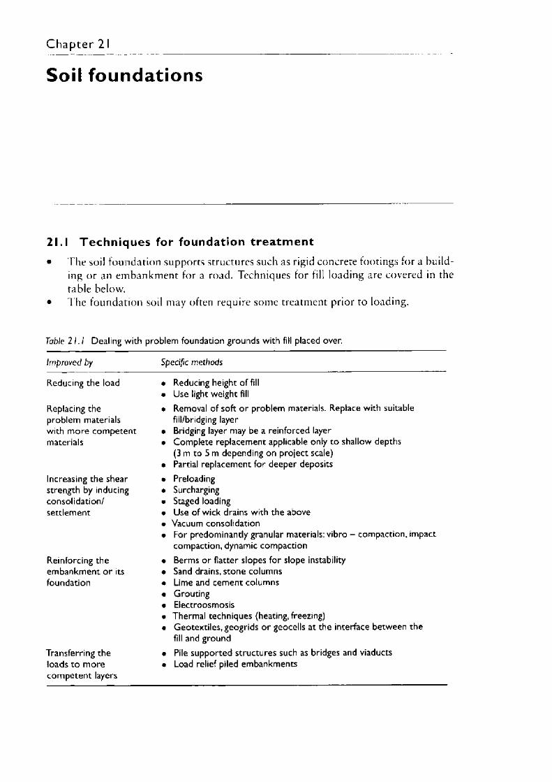
Chapter 2 1
Soil foundations
21.1 Techn iques for foundation t reatm ent• The soil foundation supports structures such as rigid concrete footings for a build
ing or an embankment for a road. Techniques for fill loading are covered in thetable below.
• The foundation soil may often require some treatment prior to loading.
Table 21.1 Dealing with problem foundation grounds with fill placed over.
Improved by Specific methods
Reducing the load • Reducing height of fill• Use light weight fill
Replacing the • Removal of soft or problem materials. Replace with suitableproblem materials fill/bridging layerwith more competent • Bridging layer may be a reinforced layermaterials • Complete replacement applicable only to shallow depths
(3 m to 5 m depending on project scale)• Partial replacement for deeper deposits
Increasing the shear • Preloadingstrength by inducing • Surchargingconsolidation/ • Staged loadingsettlement • Use of wick drains with the above
• Vacuum consolidation• For predominantly granular materials: vibro - compaction, impact
compaction, dynamic compactionReinforcing the • Berms or flatter slopes for slope instabilityembankment or its • Sand drains, stone columnsfoundation • Lime and cement columns
• Grouting• Electroosmosis• Thermal techniques (heating, freezing)• Geotextiles, geogrids or geocells at the interface between the
fill and groundTransferring the • Pile supported structures such as bridges and viaductsloads to more • Load relief piled embankmentscompetent layers
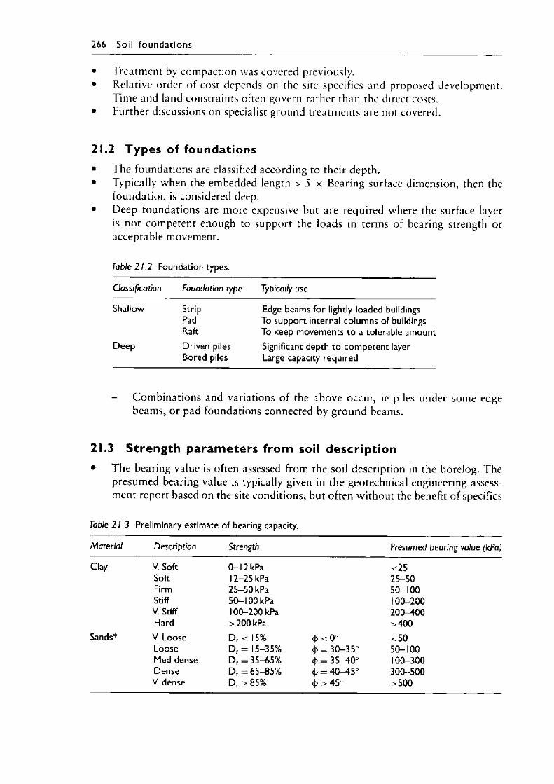
266 So il fo unda tions
• Treatment by compaction was covered previously.• Relative order of cost depends on the site specifics and proposed development.
Time and land constraints often govern rather than the direct costs.• Further discussions on specialist ground treatments are not covered.
21.2 Types of foundations• The foundations are classified according to their depth.• Typically when the embedded length > 5 x Bearing surface dimension, then the
foundation is considered deep.• Deep foundations are more expensive but are required where the surface layer
is not competent enough to support the loads in terms of bearing strength or acceptable movement.
Table 21.2 Foundation types.
Classification Foundation type Typically use
Shallow Strip Edge beams for lightly loaded buildingsPad To support internal columns of buildingsRaft To keep movements to a tolerable amount
Deep Driven piles Significant depth to competent layerBored piles Large capacity required
Combinations and variations o f the above occur, ie piles under some edge beams, or pad foundations connected by ground beams.
21.3 Strength p aram eters from soil description• The bearing value is often assessed from the soil description in the borelog. The
presumed bearing value is typically given in the geotechnical engineering assessment report based on the site conditions, but often without the benefit of specifics
Table 21.3 Preliminary estimate of bearing capacity.
Material Description Strength Presumed bearing value (kPa)
Clay V. Soft 0 -l2 k P a <25Soft 12-25 kPa 25-50Firm 25-50 kPa 50-100Stiff 50-100 kPa 100-200V. Stiff 100-200 kPa 200-400Hard >200kPa >400
Sands* V. Loose D r < 15% < 0° <50Loose D r = 15-35% 4> = 30-35° 5 0 - 100Med dense D r = 35-65% 4> = 35-40° 100-300Dense D r = 65-85% <(, = 40-45° 300-500V. dense D r > 85% 4> > 45° > 500
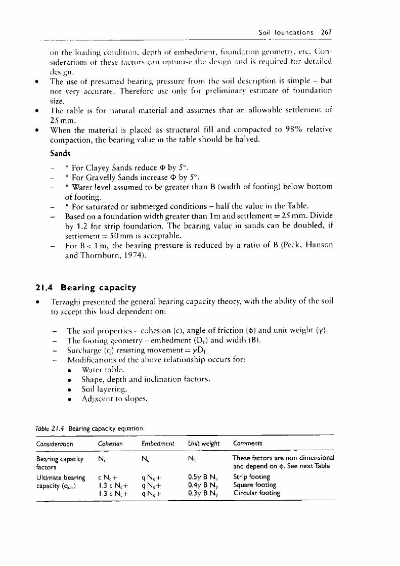
Soil fo u n d a t ion s 267
on the loading condition, depth of embedment, foundation geometry, etc. C o n siderations of these factors can optimise the design and is required for detailed design.
• The use of presumed bearing pressure from the soil description is simple - but not very accurate. Therefore use only for preliminary estimate of foundation size.
• The table is for natural material and assumes that an allowable settlement of 25 mm.
• When the material is placed as structural fill and compacted to 9 8 % relative compaction, the bearing value in the table should be halved.
Sands
- * For Clayey Sands reduce by 5°.• For Gravelly Sands increase <t> by 5°.• Water level assumed to be greater than B (width of footing) below bottom of footing.
- * For saturated or submerged conditions - half the value in the Table.Based on a foundation width greater than 1 m and settlement = 25 mm. Divide by 1.2 for strip foundation. The bearing value in sands can be doubled, if settlement = 50 mm is acceptable.
- For B < 1 m, the bearing pressure is reduced by a ratio of B (Peck, Hanson and Thornburn, 1974).
21.4 Bearing capacity• Terzaghi presented the general bearing capacity theory, with the ability o f the soil
to accept this load dependent on:
The soil properties - cohesion (c), angle o f friction (())) and unit weight (y).- The footing geometry - embedment (Df) and width (B).
Surcharge (q ) resisting movement = y D f Modifications of the above relationship occurs for:• Water table.• Shape, depth and inclination factors.• Soil layering.• Adjacent to slopes.
Table 21.4 Bearing capacity equation.
Consideration Cohesion Embedment Unit weight Comments
Bearing capacity factors
N c Nq N y These factors are non dimensional and depend on cj). See next Table
Ultimate bearing c N c + q N q+ 0.5y B N y Strip footingcapacity (quk) 1.3 c Nc + q N ,+ 0.4y B N y Square footing
1.3 c Nc + q N q + 0.3y B N y Circular footing
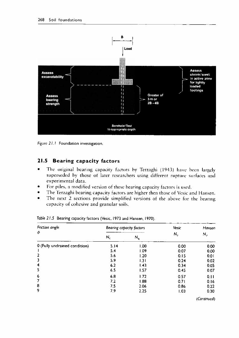
268 So il fo u n d a t io n s
B
Load
Assess shrink/swell in active zone for lightly loaded
footingsGreater of 3 m or 2 B -4 B
B orehole/Test to appropriate depth
Figure 21.1 Foundation investigation.
21.5 Bearing capac ity factors• The original bearing capacity factors by Terzaghi (1943) have been largely
superseded by those o f later researchers using different rupture surfaces and experimental data.
• For piles, a modified version of these bearing capacity factors is used.• The Terzaghi bearing capacity factors are higher then those of Vesic and Hansen.• The next 2 sections provide simplified versions of the above for the bearing
capacity o f cohesive and granular soils.
Table 21.5 Bearing capacity factors (Vesic, 1973 and Hansen, 1970).
Friction angle Bearing capacity factors Vesic Hansen<P Ny Ny
Nc Nq Y Y
0 (Fully undrained condition) 5.14 1.00 0.00 0.001 5.4 1.09 0.07 0.002 5.6 1.20 0.15 0.013 5.9 1.31 0.24 0.024 6.2 1.43 0.34 0.055 6.5 1.57 0.45 0.076 6.8 1.72 0.57 0.117 7.2 1.88 0.71 0.168 7.5 2.06 0.86 0.229 7.9 2.25 1.03 0.30
(Continued)
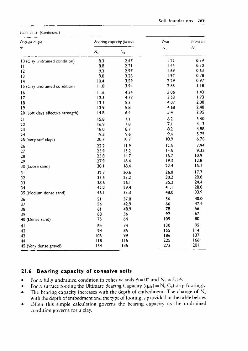
Soil fo u n d a t io n s 269
Table 2 1.5 (Continued)
Friction angle<!>
Bearing capacity factors
Nc Nq
VesicN
HansenN
10 (Clay undrained condition) 8.3 2.47 1.22 0.391 1 8.8 2.71 1.44 0.5012 9.3 2.97 1.69 0.6313 9.8 3.26 1.97 0.7814 10.4 3.59 2.29 0.9715 (Clay undrained condition) 1 1.0 3.94 2.65 1.1816 1 1.6 4.34 3.06 1.4317 12.3 4.77 3.53 1.7318 13.1 5.3 4.07 2.0819 13.9 5.8 4.68 2.4820 (Soft clays effective strength) 14.8 6.4 5.4 2.9521 15.8 7.1 6.2 3.5022 16.9 7.8 7.1 4.1323 18.0 8.7 8.2 4.8824 19.3 9.6 9.4 5.7525 (Very stiff clays) 20.7 10.7 10.9 6.7626 22.2 1 1.9 12.5 7.9427 23.9 13.2 14.5 9.3228 25.8 14.7 16.7 10.929 27.9 16.4 19.3 12.830 (Loose sand) 30.1 18.4 22.4 15.131 32.7 20.6 26.0 17.732 35.5 23.2 30.2 20.833 38.6 26.1 35.2 24.434 42.2 29.4 41.1 28.835 (Medium dense sand) 46.1 33.3 48.0 33.936 51 37.8 56 40.037 56 42.9 66 47.438 61 48.9 78 5639 68 56 92 6740 (Dense sand) 75 64 109 8041 84 74 130 9542 94 85 155 1 1443 105 99 186 13744 1 18 1 15 225 16645 (Very dense gravel) 134 135 272 201
21.6 Bearing capacity of cohesive soils• For a fully undrained condition in cohesive soils 0 = 0° and Nc = 5 .14 .• For a surface footing the Ultimate Bearing Capacity (quit) — N c C u(strip footing).• The bearing capacity increases with the depth of embedment. The change of Nc
with the depth of embedment and the type of footing is provided in the table below.• Often this simple calculation governs the bearing capacity as the undrained
condition governs for a clay.
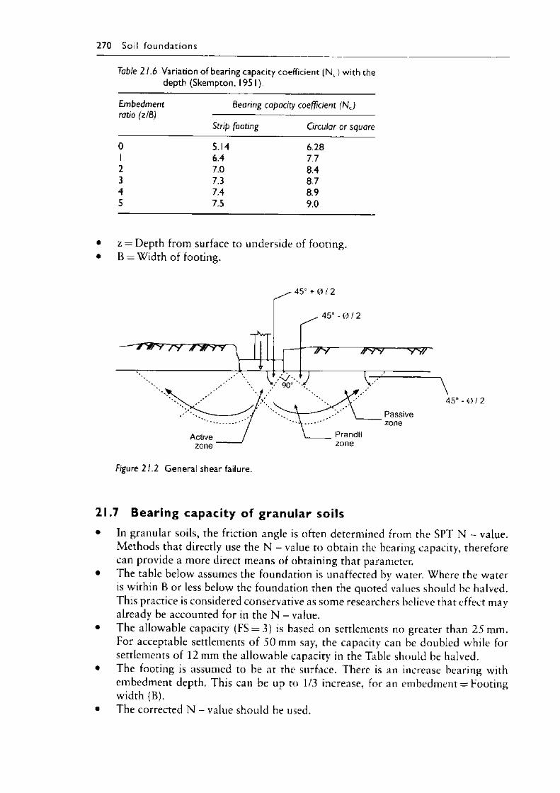
270 Soil fo undations
Table 21.6 Variation of bearing capacity coefficient ( N ,) with the depth (Skempton, 1951).
Embedment ratio (z/B)
Bearing capacity coefficient (Nc)
Strip footing Circular or square
0 5.14 6.281 6.4 7.72 7.0 8.43 7.3 8.74 7.4 8.95 7.5 9.0
• z = Depth from surface to underside of footing.• B = Width of footing.
Figure 21.2 General shear failure.
21.7 Bearing capacity of granular soils• In granular soils, the friction angle is often determined from the SPT N - value.
Methods that directly use the N - value to obtain the bearing capacity, therefore can provide a more direct means of obtaining that parameter.
• The table below assumes the foundation is unaffected by water. Where the water is within B or less below the foundation then the quoted values should be halved. This practice is considered conservative as some researchers believe that effect may already be accounted for in the N - value.
• The allowable capacity (FS = 3) is based on settlements no greater than 2 5 mm. For acceptable settlements o f 50 mm say, the capacity can be doubled while for settlements of 12 mm the allowable capacity in the Table should be halved.
• The footing is assumed to be at the surface. There is an increase bearing with embedment depth. This can be up to 1/3 increase, for an embedment = Footing width (B).
• The corrected N - value should be used.
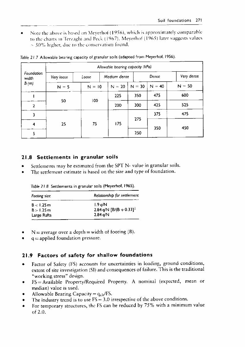
Soil fo u n d a t io n s 271
• Note the above is based on Meyerhof (1 956) , which is approximately comparable ro the charts in Ter/.aghi and Peck (1967). Meyerhof (1965) later suggests values— 5 0 % higher, due to the conservatism found.
Table 21.7 Allowable bearing capacity of granular soils (adapted from Meyerhof, 1956).
FoundationwidthB (m)
Allowable bearing capacity (kPa)
Very loose Loose Medium dense Dense Very dense
N = 5 N = 10 N = 20 N = 30oIIZ N = 50
150 100
225 350 475 600
2 200 300 425 525
3
25 75 175275
375 475
4350 450
5 250
21.8 Sett lem ents in granular soils• Settlements may be estimated from the SPT N- value in granular soils.• The settlement estimate is based on the size and type of foundation.
Table 21.8 Settlements in granular soils (Meyerhof, 1965).
Footing size Relationship for settlement
B < 1.25 m 1.9 q/NB> 1.25 m 2.84 q/N [B/(B + 0.33]2Large Rafts 2.84 q/N
• N = average over a depth = width of footing (B).• q = applied foundation pressure.
21.9 Factors of safety for shallow foundations• Factor of Safety (FS) accounts for uncertainties in loading, ground conditions,
extent o f site investigation (SI) and consequences of failure. This is the traditional“working stress” design.
• FS = Available Property/Required Property. A nominal (expected, mean or median) value is used.
• Allowable Bearing Capacity = quit/FS.• The industry trend is to use FS = 3 .0 irrespective of the above conditions.• For temporary structures, the FS can be reduced by 7 5 % with a minimum value
of 2 .0 .
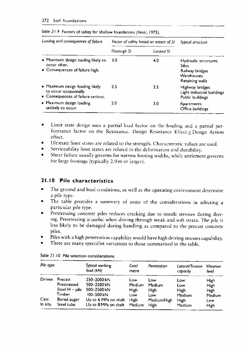
272 Soil foundations
Table 21.9 Factors of safety for shallow foundations (Vesic, 1975).
Loading and consequences o f failure Factor o f safety based
Thorough SI
on extent o f SI
Limited SI
Typical structure
• Maximum design loading likely to occur often.
• Consequences of failure high.
3.0 4.0 Hydraulic structures SilosRailway bridges Warehouses Retaining walls
• Maximum design loading likely to occur occasionally.
• Consequences of failure serious.
2.5 3.5 Highway bridges Light industrial buildings Public buildings
• Maximum design loading unlikely to occur.
2.0 3.0 Apartments Office buildings
• Limit state design uses a partial load factor on the loading and a partial performance factor on the Resistance. Design Resistance Effect > Design Action effect.
• Ultimate limit states are related to the strength. Characteristic values are used.• Serviceability limit states are related to the deformation and durability.• Shear failure usually governs for narrow footing widths, while settlement governs
for large footings (typically 2 .0 m or larger).
21.10 Pile character ist ics• The ground and load conditions, as well as the operating environment determine
a pile type.• The table provides a summary of some of the considerations in selecting a
particular pile type.• Prestressing concrete piles reduces cracking due to tensile stresses during driv
ing. Prestressing is useful when driving through weak and soft strata. The pile is less likely to be damaged during handling as compared to the precast concrete piles.
• Piles with a high penetration capability would have high driving stresses capability.• There are many specialist variations to those summarised in the table.
Table 21.10 Pile selection considerations.
Pile type Typical working load (kN)
Cost/metre
Penetration Lateral/Tensioncapacity
Vibrationlevel
Driven Precast 250-2000 kN Low Low Low HighPrestressed 500-2500 kN Medium Medium Low HighSteel H - pile 500-2500 kN High High High HighTimber 100-500 kN Low Low Medium Medium
Cast Bored auger Up to 6 MPa on shaft High Medium/High High LowIn situ Steel tube Up to 8 MPa on shaft Medium High Medium High
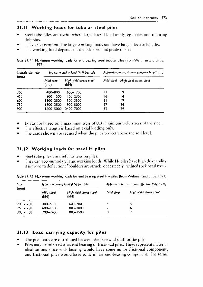
Soil founda tions 273
21.11 W o rk in g loads for tubular steel piles• Steel tube piles arc useful where large lateral load apply, eg jetties and mooring
dolphins.• They can accomm odate large working loads and have large effective lengths.• The working load depends on the pile size, and grade of steel.
Table 21.11 Maximum working loads for end bearing steel tubular piles (from Weltman and Little, 1977).
Outside diameter Typical working load (kN) per pile Approximate maximum effective length (m)
M ild steel (kN)
High yield stress steel (kN)
Mild steel High yield stress steel
300 400-800 600-1200 1 1 9450 800-1500 1100-2300 16 14600 1100-2500 1500-3500 21 19750 1300-3500 i 900-5000 27 24900 1600-5000 2400-7000 32 29
• Loads are based on a maximum tress of 0..3 x minium yield stress of the steel.• The effective length is based on axial loading only.• The loads shown are reduced when the piles project above the soil level.
21.12 W o rk in g loads for steel H piles• Steel tube piles are useful as tension piles.• They can accom m odate large working loads. While H- piles have high driveability,
it is prone to deflection if boulders are struck, or at steeply inclined rock head levels.
Table 21.12 Maximum working loads for end bearing steel H - piles (from Weltman and Little, 1977).
Size(mm)
Typical working load (kN) per pile Approximate maximum effective length (m)
Mild steel (kN)
High yield stress steel (kN)
Mild steel High yield stress steel
200 x 200 400-500 600-700 5 4250 x 250 600-1500 800-2000 7 6300 x 300 700-2400 1000-3500 8 7
21.13 Load carry ing capacity for piles• The pile loads are distributed between the base and shaft of the pile.• Piles may be referred to as end bearing or frictional piles. These represent material
idealisations since end- bearing would have some minor frictional component, and frictional piles would have some minor end-bearing component. The terms
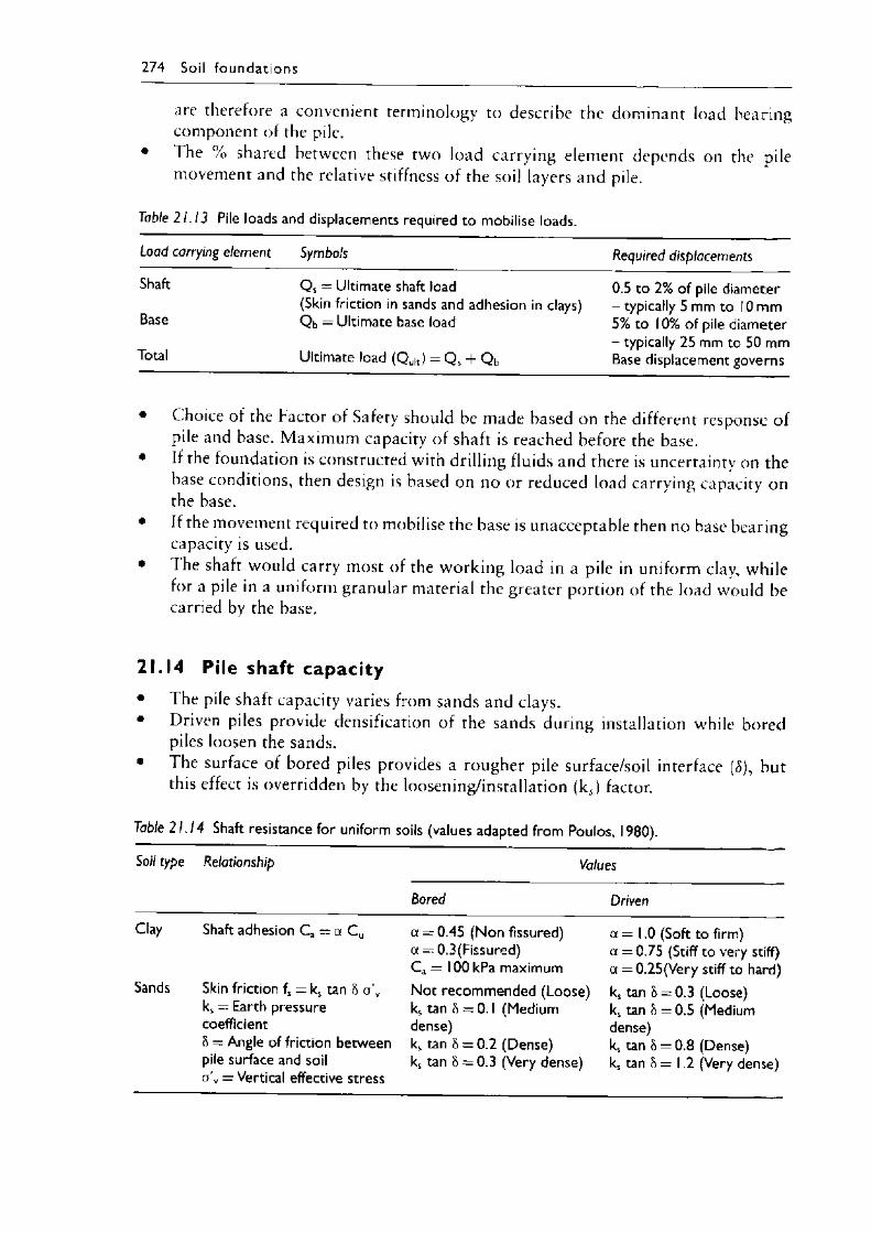
274 Soil founda t ions
arc therefore a convenient terminology to describe the dominant load bearing component of the pile.
• The % shared between these two load carrying element depends on the pile movement and the relative stiffness of the soil layers and pile.
Table 21.13 Pile loads and displacements required to mobilise loads.
Load carrying element Symbols Required displacements
Shaft Q s = Ultimate shaft load 0.5 to 2% of pile diameter(Skin friction in sands and adhesion in clays) - typically 5 mm to 10 mm
Base Q b = Ultimate base load 5% to 10% of pile diameter- typically 25 mm to 50 mm
Total Ultimate load (Q uk) = Q s + Q b Base displacement governs
• Choice of the Factor o f Safety should be made based on the different response o f pile and base. Maximum capacity o f shaft is reached before the base.
• If the foundation is constructed with drilling fluids and there is uncertainty on the base conditions, then design is based on no or reduced load carrying capacity on the base.
• If the movement required to mobilise the base is unacceptable then no base bearing capacity is used.
• The shaft would carry most of the working load in a pile in uniform clay, while for a pile in a uniform granular material the greater portion of the load would be carried by the base.
21.14 Pile shaft capacity• The pile shaft capacity varies from sands and clays.• Driven piles provide densification o f the sands during installation while bored
piles loosen the sands.• The surface of bored piles provides a rougher pile surface/soil interface (<$), but
this effect is overridden by the loosening/installation (ks) factor.
Table 21.14 Shaft resistance for uniform soils (values adapted from Poulos, 1980).
Soil type Relationship Values
Bored Driven
Clay Shaft adhesion C a = a C u a = 0.45 (Non fissured) a — 0.3(Fissured)C a = 100 kPa maximum
a = 1.0 (Soft to firm) a = 0.75 (Stiff to very stiff) a = 0.25(Very stiff to hard)
Sands Skin friction f5 = ks tan 8 o 'v ks = Earth pressure coefficient& = Angle of friction betweenpile surface and soila'v = Vertical effective stress
Not recommended (Loose) ks tan 8 = 0.1 (Medium dense)ks tan 8 = 0.2 (Dense) ks tan 8 = 0.3 (Very dense)
ks tan 8 = 0.3 (Loose) ks tan 8 = 0.5 (Medium dense)ks tan 8 = 0.8 (Dense) ks tan 8 = 1 .2 (Very dense)
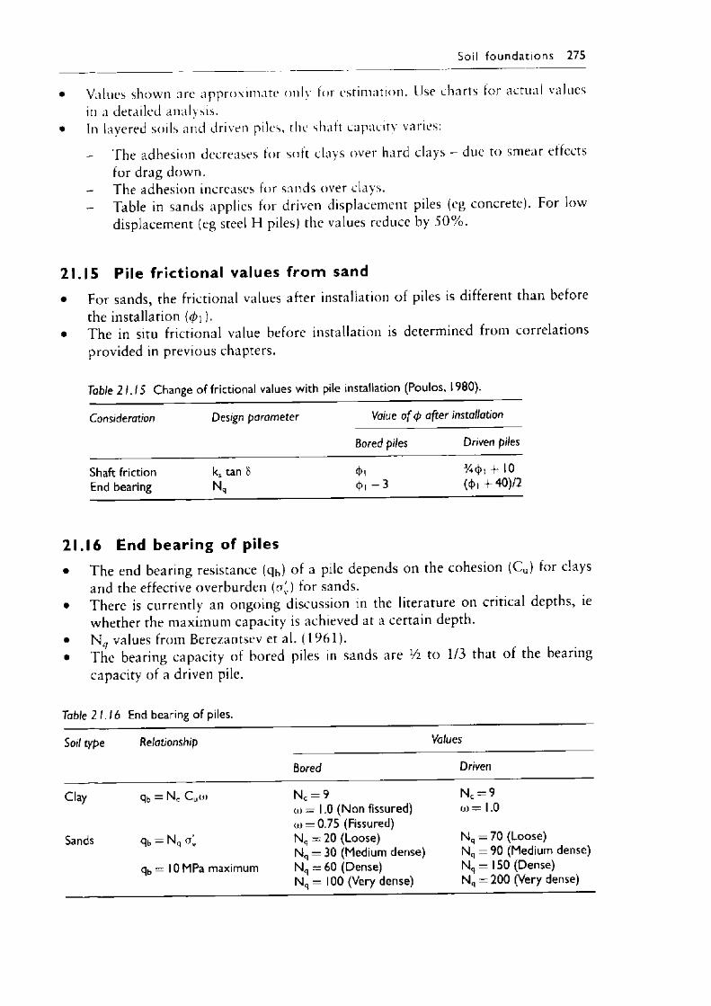
Soil fo u n d a t io n s 275
• Values shown are approximate only for estimation. Use charts for actual values in a detailed analysis.
• In layered soils and driven piles, the shaft capacity varies:
- The adhesion decreases for soft clays over hard clays — due to smear effectsfor drag down.
- The adhesion increases for sands over clays.- Table in sands applies for driven displacement piles (eg concrete). For low
displacement (eg steel FI piles) the values reduce by 5 0 % .
21.15 Pile fr ictional values from sand• For sands, the frictional values after installation of piles is different than before
the installation (</>i ).• The in situ frictional value before installation is determined from correlations
provided in previous chapters.
Table 21.15 Change of frictional values with pile installation (Poulos, 1980).
Consideration Design parameter Value o f (p after installation
Bored piles Driven piles
Shaft friction ks tan h <t>i 3/4<l>| + 10End bearing N„ <t>i - 3 (<t>i + 40)/2
21.16 End bearing of piles• The end bearing resistance (cjh) of a P^e depends on the cohesion (C u) for clays
and the effective overburden (ex') for sands.• There is currently an ongoing discussion in the literature on critical depths, ie
whether the maximum capacity is achieved at a certain depth.• N4/ values from Berezantsev et al. (1961).• The bearing capacity of bored piles in sands are Vi to 1/3 that of the bearing
capacity of a driven pile.
Table 21.16 End bearing of piles.
Soil type Relationship Values
Bored Driven
Clay
Sands
qb = N c C uo>
qb = N q a ;
qb = 10 MPa maximum
N c = 9o )= 1.0 (Non fissured)03 = 0.75 (Fissured)N q = 20 (Loose)N q = 30 (Medium dense) N q = 60 (Dense)N q — 100 (Very dense)
N c = 9oo= 1.0
N q = 70 (Loose)N q = 90 (Medium dense) N q = 150 (Dense)N q = 200 (Very dense)
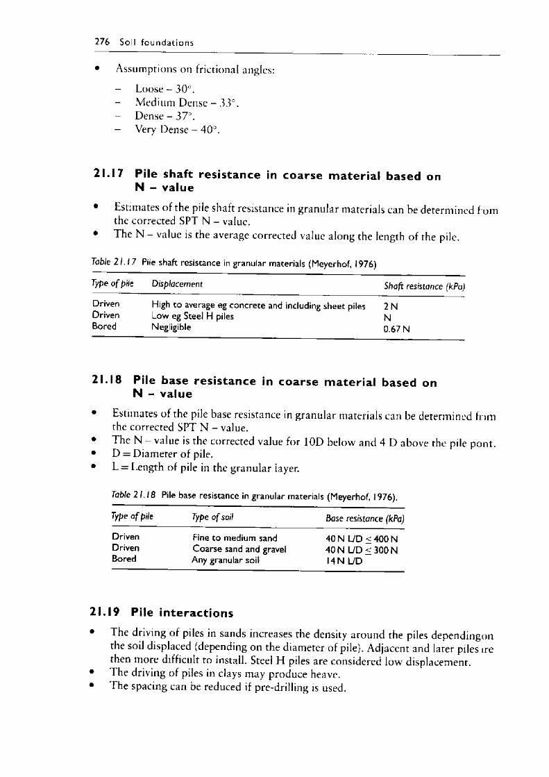
276 Soil founda tions
• Assumptions on frictional angles:
- Loose - 30°.Medium Dense - 33°.Dense - 37°.Very Dense - 40°.
21.17 Pile shaft resistance in coarse materia l based on N - value
• Estimates o f the pile shaft resistance in granular materials can be determined f om the corrected SPT N - value.
• The N - value is the average corrected value along the length of the pile.
Table 21.17 Pile shaft resistance in granular materials (Meyerhof, 1976)
Type o f pile Displacement Shaft resistance (kPa)
Driven High to average eg concrete and including sheet piles 2NDriven Low eg Steel H piles NBored Negligible 0.67 N
21.18 Pile base resistance in coarse m ateria l based on N - value
• Estimates o f the pile base resistance in granular materials can be determined fnm the corrected SPT N - value.
• The N - value is the corrected value for 10D below and 4 D above the pile pont.• D = Diameter o f pile.• L = Length o f pile in the granular layer.
Table 21.18 Pile base resistance in granular materials (Meyerhof, 1976).
Type o f pile Type o f soil Base resistance (kPa)
Driven Fine to medium sand 40 N L/D < 400 NDriven Coarse sand and gravel 40 N L/D < 300 NBored Any granular soil 14 N L/D
21.19 Pile interactions• The driving o f piles in sands increases the density around the piles dependingon
the soil displaced (depending on the diameter of pile). Adjacent and later piles irethen more difficult to install. Steel H piles are considered low displacement.
• The driving o f piles in clays may produce heave.• The spacing can be reduced if pre-drilling is used.
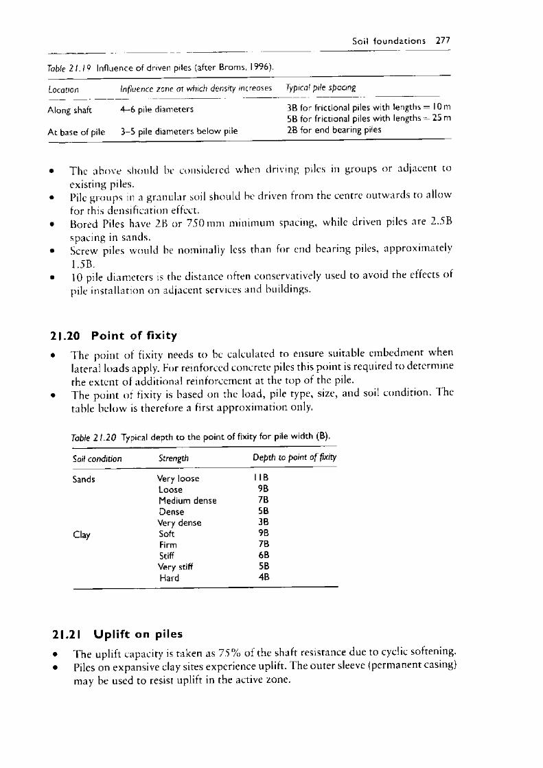
Soil fou n d a t ion s 277
Table 21.19 Influence of driven piles (after Broms, 1996).
Location Influence zone at which density increases Typical pile spacing
Along shaft
At base of pile
4-6 pile diameters
3-5 pile diameters below pile
3B for frictional piles with lengths = 10 m 5B for frictional piles with lengths = 25 m 2B for end bearing piles
• The above should he considered when driving piles in groups or adjacent to existing piles.
• Pile groups in a granular soil should be driven from the centre outwards to allow for this densification effect.
• Bored Piles have 2B or 7 5 0 mm minimum spacing, while driven piles are 2.5Bspacing in sands.
• Screw piles would he nominally less than for end hearing piles, approximately 1.5B.
• 10 pile diameters is the distance often conservatively used to avoid the effects of pile installation on adjacent services and buildings.
21.20 Point of fixity• The point of fixity needs to be calculated to ensure suitable embedment when
lateral loads apply. For reinforced concrete piles this point is required to determine the extent of additional reinforcement at the top of the pile.
• The point of fixity is based on the load, pile type, size, and soil condition. The table below is therefore a first approximation only.
Table 21 .20 Typical depth to the point of fixity for pile width (B).
Soil condition Strength Depth to point o f fixity
Sands Very loose 1 IBLoose 9BMedium dense 7BDense 5BVery dense 3B
Clay Soft 9BFirm 7BStiff 6BVery stiff 5BHard 4B
21.21 Uplift on piles• The uplift capacity is taken as 7 5 % of the shaft resistance due to cyclic softening.• Piles on expansive clay sites experience uplift. The outer sleeve (permanent casing)
may be used to resist uplift in the active zone.
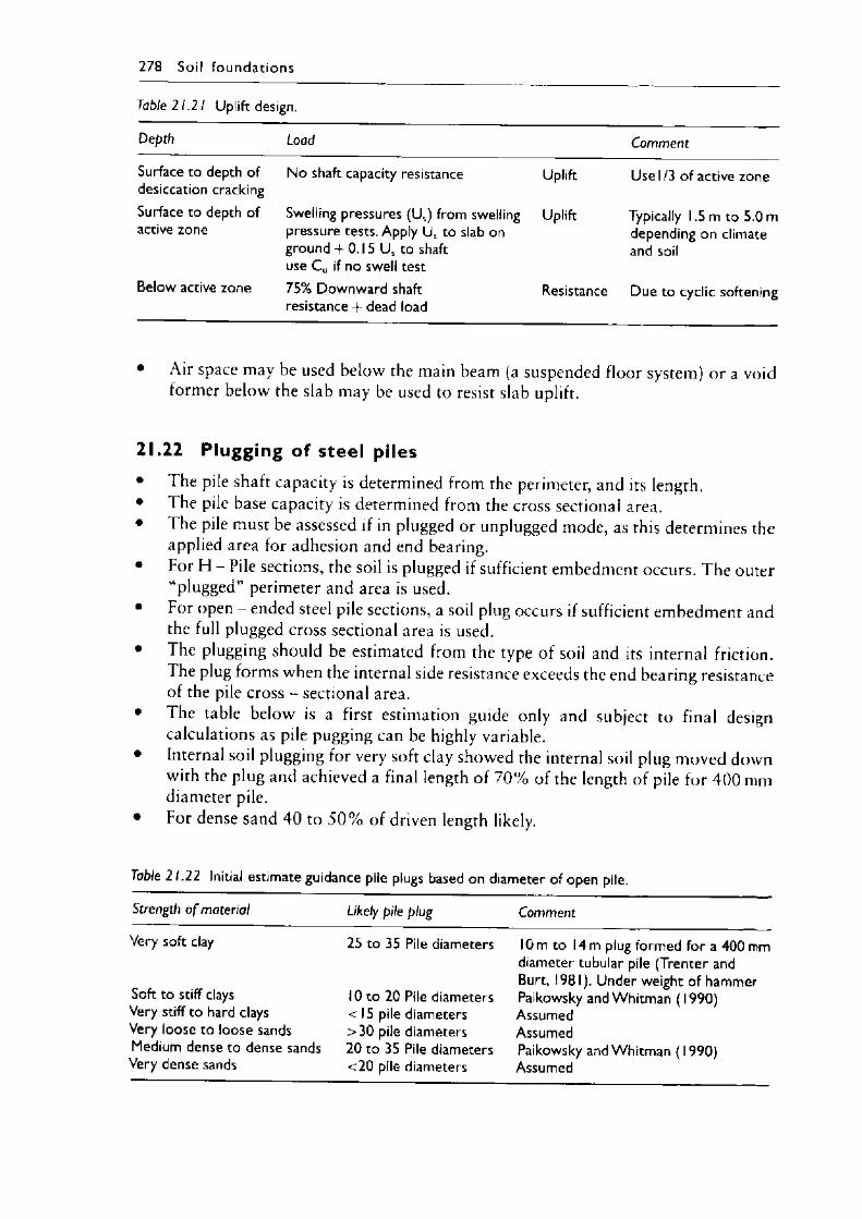
278 Soil foundat ions
Table 21.21 Uplift design.
Depth Load Comment
Surface to depth of desiccation cracking
No shaft capacity resistance Uplift Use 1/3 of active zone
Surface to depth of active zone
Swelling pressures (Us) from swelling pressure tests. Apply U s to slab on ground + 0.15 U s to shaft use C u if no swell test
Uplift Typically 1.5 m to 5.0 m depending on climate and soil
Below active zone 75% Downward shaft resistance + dead load
Resistance Due to cyclic softening
• Air space may be used below the main beam (a suspended floor system) or a void former below the slab may be used to resist slab uplift.
21.22 Plugging of steel piles• The pile shaft capacity is determined from the perimeter, and its length.• The pile base capacity is determined from the cross sectional area.• The pile must be assessed if in plugged or unplugged mode, as this determines the
applied area for adhesion and end bearing.• For H - Pile sections, the soil is plugged if sufficient embedment occurs. The outer
“ plugged” perimeter and area is used.• For open - ended steel pile sections, a soil plug occurs if sufficient embedment and
the full plugged cross sectional area is used.• The plugging should be estimated from the type of soil and its internal friction.
The plug forms when the internal side resistance exceeds the end bearing resistance of the pile cross - sectional area.
• The table below is a first estimation guide only and subject to final designcalculations as pile pugging can be highly variable.
• Internal soil plugging for very soft clay showed the internal soil plug moved down with the plug and achieved a final length of 7 0 % of the length of pile for 4 0 0 mm diameter pile.
• For dense sand 4 0 to 5 0 % of driven length likely.
Table 21.22 Initial estimate guidance pile plugs based on diameter of open pile.
Strength o f material Likely pile plug Comment
Very soft clay
Soft to stiff clays Very stiff to hard clays Very loose to loose sands Medium dense to dense sands
Very dense sands
25 to 35 Pile diameters
10 to 20 Pile diameters < 15 pile diameters >30 pile diameters 20 to 35 Pile diameters <20 pile diameters
10 m to 14m plug formed for a 400 mm diameter tubular pile (Trenter and Burt, 1981). Under weight of hammer Paikowsky and Whitman (1990) Assumed AssumedPaikowsky and Whitman (1990) Assumed
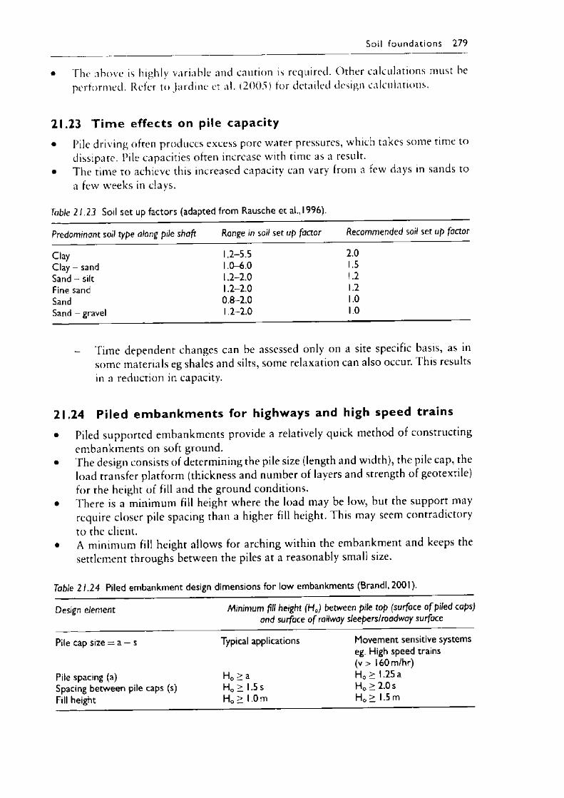
Soil founda tions 279
• The above is highly variable and caution is required. Other calculations must beperformed. Refer to Jardine et al. (2005) for detailed design calculations.
21.23 T im e effects on pile capacity• Pile driving often produces excess pore water pressures, which takes some time to
dissipate. Pile capacities often increase with time as a result.• The time to achieve this increased capacity can vary from a few days in sands to
a few weeks in clays.
Table 21.23 Soil set up factors (adapted from Rausche et al., 1996).
Predominant soil type along pile shaft Range in soil set up factor Recommended soil set up factor
Clay 1.2-5.5 2.0Clay - sand 1.0-6.0 1.5Sand - silt 1.2-2.0 1.2Fine sand 1.2-2.0 1.2Sand 0.8-2.0 1.0Sand - gravel 1.2-2.0 1.0
- Time dependent changes can be assessed only on a site specific basis, as in some materials eg shales and silts, some relaxation can also occur. This results in a reduction in capacity.
21.24 Piled em bankm ents for highways and high speed trains• Piled supported embankments provide a relatively quick method of constructing
embankments on soft ground.• The design consists of determining the pile size (length and width), the pile cap, the
load transfer platform (thickness and number of layers and strength of geotextile) for the height of fill and the ground conditions.
• There is a minimum fill height where the load may be low, but the support may require closer pile spacing than a higher fill height. This may seem contradictory to the client.
• A minimum fill height allows for arching within the embankment and keeps the settlement throughs between the piles at a reasonably small size.
Table 21.24 Piled embankment design dimensions for low embankments (Brandi, 2001).
Design element Minimum fill height (H 0) between pile top (surface o f piled caps)and surface o f railway sleepers/roadway surface
Pile cap size = a - s
Pile spacing (a)Spacing between pile caps (s)Fill height
Typical applications Movement sensitive systemseg. High speed trains (v > 160 m/hr)
H0 > a H0 >1.25 aH0 > 1.5 s H0 > 2.0 sHq > 1.0 m H0 > 1.5 m
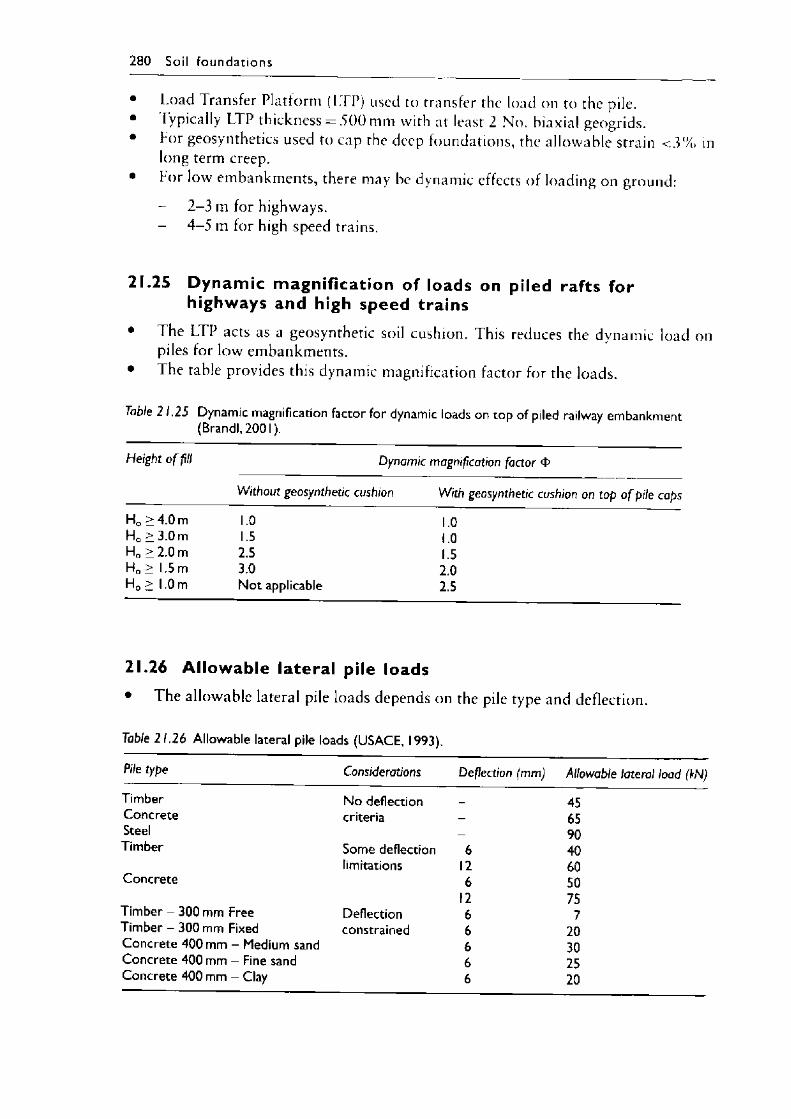
280 Soil founda t ions
• Load Transfer Platform (LTP) used to transfer the load on to the pile.• Typically LTP thickness = 5 0 0 mm with at least 2 No. biaxial geogrids.• For geosynthetics used to cap the deep foundations, the allowable strain < 3 % in
long term creep.• For low embankments, there may be dynamic effects of loading on ground:
- 2 - 3 m for highways.4 - 5 m for high speed trains.
21.25 Dynam ic magnif ication of loads on piled rafts for highways and high speed trains
• The LTP acts as a geosynthetic soil cushion. This reduces the dynamic load on piles for low embankments.
• The table provides this dynamic magnification factor for the loads.
Table 21.25 Dynamic magnification factor for dynamic loads on top of piled railway embankment (Brandi, 2001).
Height o f fill Dynamic magnification factor
Without geosynthetic cushion With geosynthetic cushion on top o f pile caps
H0 > 4.0 m 1.0 1.0H0 > 3.0 m 1.5 1.0H0 > 2.0 m 2.5 1.5H0 > 1.5 m 3.0 2.0H0 > 1.0 m Not applicable 2.5
21.26 Allowable lateral pile loads• The allowable lateral pile loads depends on the pile type and deflection.
Table 21.26 Allowable lateral pile loads (USACE, 1993).
Pile type Considerations Deflection (mm) Allowable lateral load (l>N)
Timber No deflection 45Concrete criteria — 65Steel — 90Timber Some deflection 6 40
limitations 12 60Concrete 6 50
12 75Timber - 300 mm Free Deflection 6 7Timber - 300 mm Fixed constrained 6 20Concrete 400 mm - Medium sand 6 30Concrete 400 mm - Fine sand 6 25Concrete 400 mm - Clay 6 20
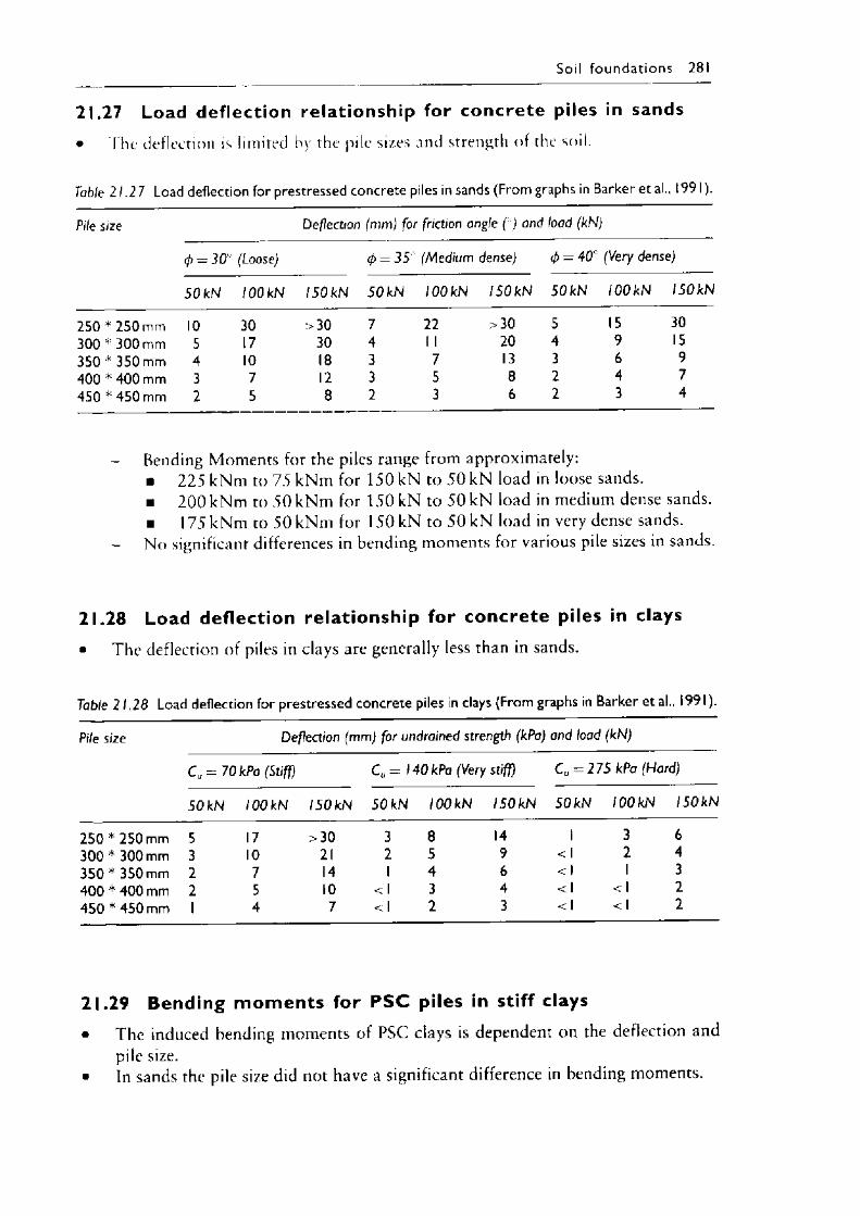
Soil fo u n d a t io n s 28
21.27 Load deflection relationship for concrete piles in sands• The deflection is limited by the pile sizes and strength of the soil.
Table 21.27 Load deflection for prestressed concrete piles in sands (From graphs in Barker et al., 19 9 1).
Pile size Deflection (mm) for friction angle ( ) and load (kN)
(f) = 30 (Loose) -e- II Uj On (Medium dense) (p == 40° (Very dense)
5 0 kN 100kN 1 50 kN 50 kN lOOkN l5 0 k N 5 0 kN lOOkN l5 0 k N
250 * 250 mm 10 30 >30 7 22 >30 5 15 30300 * 300 mm 5 17 30 4 1 1 20 4 9 15350 * 350 mm 4 10 18 3 7 13 3 6 9400 * 400 mm 3 7 12 3 5 8 2 4 7450 * 450 mm 2 5 8 2 3 6 2 3 4
Rending Moments for the piles range from approximately:■ 225 kNm to 75 kNm for 150 kN to 50 kN load in loose sands.■ 2 0 0 kNm to 50 kNm for 150 kN to 50 kN load in medium dense sands.■ 175 kNm to 50 kNm for 1 5 0 k N to 50 kN load in very dense sands.No significant differences in bending moments for various pile sizes in sands.
21.28 Load deflection relationship for concrete piles in clays• The deflection of piles in clays are generally less than in sands.
Table 2 1.28 Load deflection for prestressed concrete piles in clays (From graphs in Barker et al., 19 9 1).
Pile size Deflection (mm) for undrained strength (kPa) and load (kN)
Cu = 70kPa (Stiff) Cu = 140 kPa (Very stiff) Cu = 275 kPa (Hard)
50 kN 100 kN 150 kN 5 0 kN lOOkN l5 0 k N 5 0 kN 100kN l5 0 k N
250 * 250 mm 5 17 >30 3 8 14 1 3 6300 * 300 mm 3 10 21 2 5 9 <1 2 4350 * 350 mm 2 7 14 1 4 6 <1 1 3400 * 400 mm 2 5 10 <1 3 4 <1 <1 2450 * 450 mm 1 4 7 <1 2 3 <1 <1 2
21.29 Bending m om ents for P S C piles in stiff clays• The induced bending moments of PSC clays is dependent on the deflection and
pile size.• In sands the pile size did not have a significant difference in bending moments.
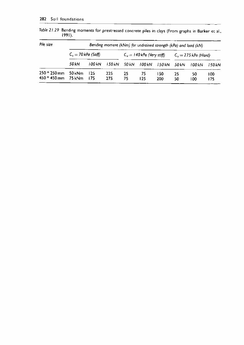
282 Soil foundations
Table 21.29 Bending moments for prestressed concrete piles in clays (From graphs in Barker et al., 1991).
Pile size Bending moment (kNm) for undrained strength (kPa) and load (kN)
Cu = 70 kPa (Stiff) Cu = 140 kPa (Very stiff) Cu = 275 kPa (Hard)
50 kN lOOkN l5 0 k N 5 0 kN lOOkN l5 0 k N 5 0 k N lOOkN l5 0 k N
250 * 250 mm 50 kNm 450 *4 5 0 mm 75 kNm
125175
225 25 75 150 25 50 100 275 75 125 200 50 100 175
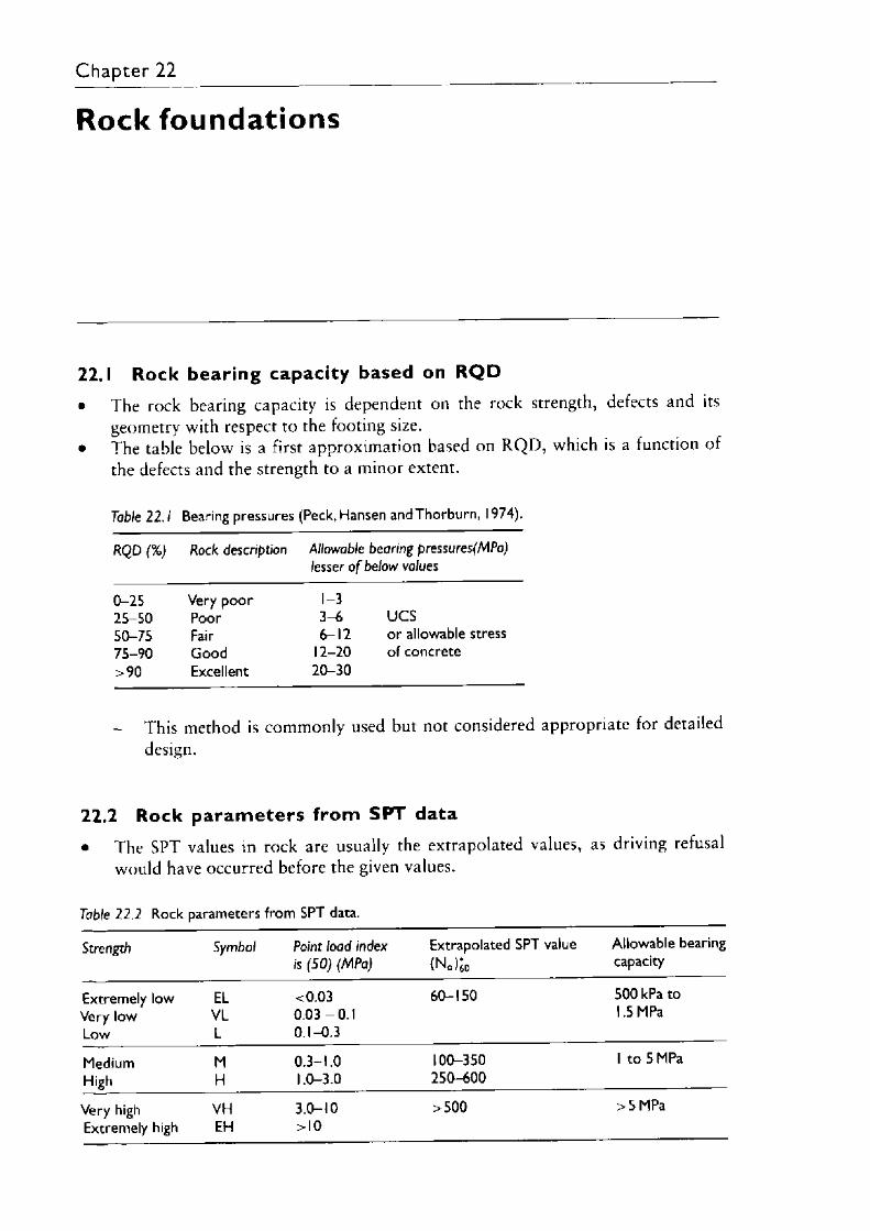
Rock foundations
22.1 Rock bearing capacity based on R Q D• The rock bearing capacity is dependent on the rock strength, defects and its
geometry with respect to the footing size.• The table below is a first approximation based on R Q D , which is a function of
the defects and the strength to a minor extent.
Table 22 .1 Bearing pressures (Peck, Hansen andThorburn, 1974).
RQD (%) Rock description Allowable bearing pressures(MPa) lesser o f below values
0-25 Very poor 1-325-50 Poor 3-6 UCS50-75 Fair 6-12 or allowable stress75-90 Good 12-20 of concrete>90 Excellent 20-30
- This method is commonly used but not considered appropriate for detailed design.
22.2 Rock p aram eters from SPT data• The SPT values in rock are usually the extrapolated values, as driving refusal
would have occurred before the given values.
Table 22.2 Rock parameters from SPT data.
Strength Symbol Point load index is (SO) (MPa)
Extrapolated SPT value(No >60
Allowable bearing capacity
Extremely low EL <0.03 60-150 500 kPa toVery low VL 0 .0 3 -0 .1 1.5 MPaLow L 0.1-0.3
Medium M 0.3-1.0 100-350 1 to 5 MPaHigh H 1.0-3.0 250-600
Very high VH 3.0-10 >500 >5 MPaExtremely high EH >10
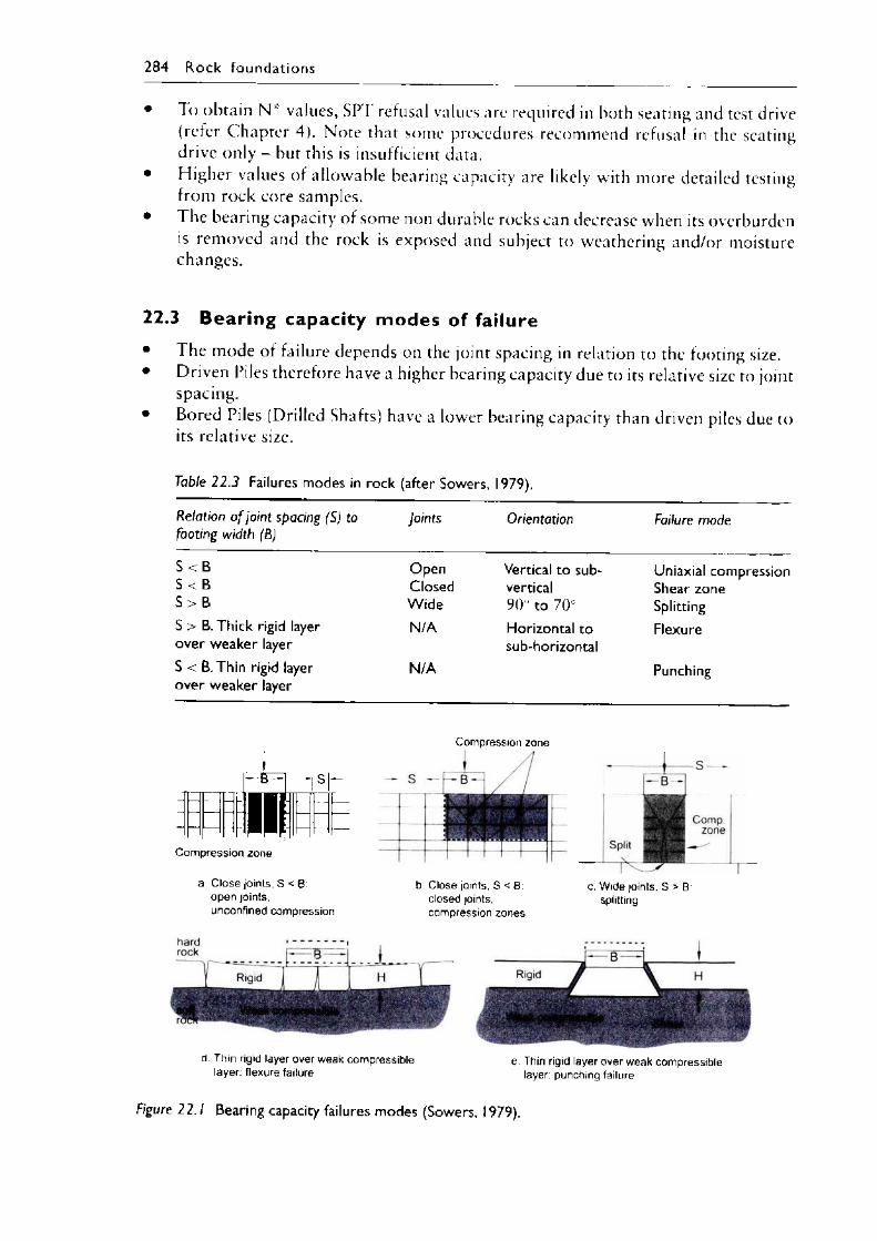
284 R o c k fo und a tio ns
• Io obtain N" values, SPT refusal values are required in both seating and test drive (refer Chapter 4). Note that some procedures recommend refusal in the seating drive only - but this is insufficient data.
• Higher values of allowable bearing capacity are likely with more detailed testing from rock core samples.
• The bearing capacity of some non durable rocks can decrease when its overburden is removed and the rock is exposed and subject to weathering and/or moisture changes.
22.3 Bearing capacity modes of failure• The mode of failure depends on the joint spacing in relation to the footing size.• Driven Piles therefore have a higher bearing capacity due to its relative size to joint
spacing.• Bored Piles (Drilled Shafts) have a lower bearing capacity than driven piles due to
its relative size.
Table 22.3 Failures modes in rock (after Sowers, 1979).
Relation o f joint spacing (S) to footing width (B)
Joints Orientation Failure mode
S < B Open Vertical to sub Uniaxial compressionS < B Closed vertical Shear zoneS > B Wide 90° to 70° SplittingS > B. Thick rigid layer over weaker layer
N/A Horizontal to sub-horizontal
Flexure
S < B. Thin rigid layer over weaker layer
N/A Punching
F T F ^ l S
Compression zone
a Close joints, S < B open joints,unconfined compression
b Close joints. S < B closed joints, compression zones
c Wide joints. S > B splitting
Compression zone
d Thin rigid layer over weak compressible layer, flexure failure
e Thin rigid layer over weak compressible layer: punching failure
Figure 2 2 .1 Bearing capacity failures modes (Sowers, 1979).
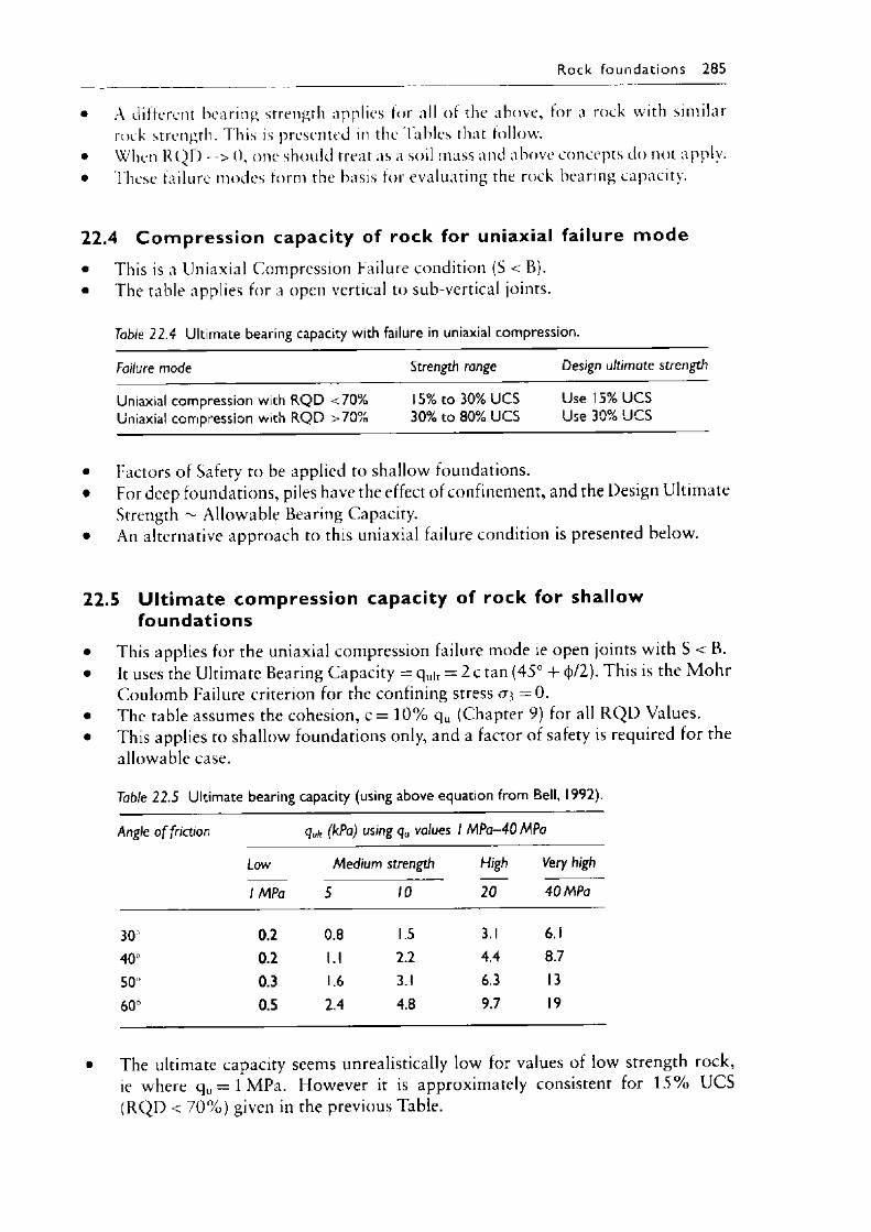
• A different hearing strength applies for all of the above, for a rock with similar rock strength. This is presented in the Tables that follow.
• When R Q D --> 0, one should treat as a soil mass and above concepts do not apply.• These failure modes form the basis for evaluating the rock bearing capacity.
22.4 C om press io n capacity of rock for uniaxial failure mode• This is a Uniaxial Compression Failure condition (S < B).• The table applies for a open vertical to sub-vertical joints.
R o c k fo u n d a t io n s 285
Table 22.4 Ultimate bearing capacity with failure in uniaxial compression.
Failure mode Strength range Design ultimate strength
Uniaxial compression with R Q D <70% Uniaxial compression with R Q D >70%
15% to 30% UCS 30% to 80% UCS
Use 15% U CS Use 30% U CS
• Factors of Safety to be applied to shallow foundations.• For deep foundations, piles have the effect of confinement, and the Design Ultimate
Strength ~ Allowable Bearing Capacity.• An alternative approach to this uniaxial failure condition is presented below.
22.5 U lt im ate com press ion capacity of rock for shallow foundations
• This applies for the uniaxial compression failure mode ie open joints with S < B.• It uses the Ultimate Bearing Capacity = q u|r — 2 c tan (45° + 4>/2). This is the M oh r
Coulomb Failure criterion for the confining stress <7* = 0.• The table assumes the cohesion, c = 1 0 % q L1 (Chapter 9) for all R Q D Values.• This applies to shallow foundations only, and a factor of safety is required for the
allowable case.
Table 22.5 Ultimate bearing capacity (using above equation from Bell, 1992).
Angle o f friction qull (kPa) using qu values I M Pa-40 MPa
Low Medium strength High Very high
1 MPa 5 10 20 40 MPa
30 0.2 0.8 1.5 3.1 6.140 0.2 l.l 2.2 4.4 8.750 0.3 1.6 3.1 6.3 1360 0.5 2.4 4.8 9.7 19
• The ultimate capacity seems unrealistically low for values of low strength rock, ie where q u = 1 MPa. However it is approximately consistent for 1 5 % UCS (RQ D < 7 0 % ) given in the previous Table.
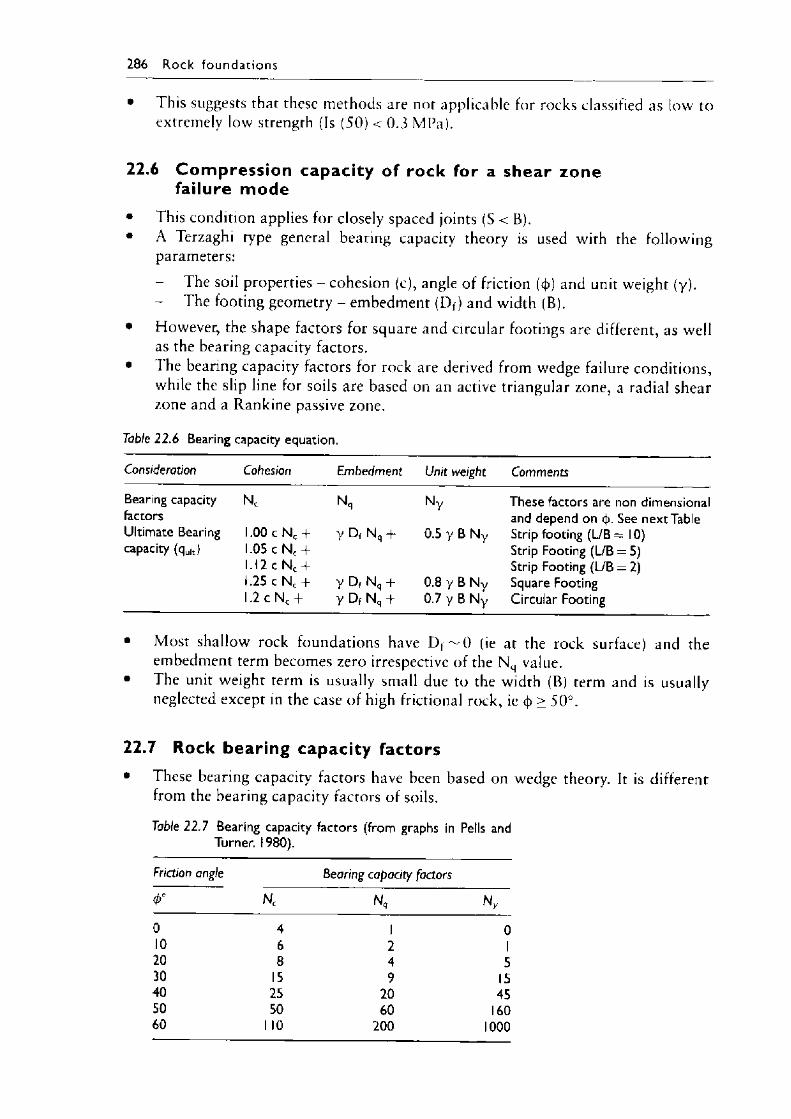
286 R o ck founda tions
• This suggests that these methods are not applicable for rocks classified as low to extremely low strength (Is (50) < 0.3 MPa).
22.6 C om press ion capacity of rock for a shear zone failure mode
• This condition applies for closely spaced joints (S < B).• A Terzaghi type general bearing capacity theory is used with the following
parameters:
- The soil properties - cohesion (c), angle of friction (<\>) and unit weight (y).- The footing geometry - embedment ( D f ) and width ( B ) .
• However, the shape factors for square and circular footings are different, as well as the bearing capacity factors.
• The bearing capacity factors for rock are derived from wedge failure conditions, while the slip line for soils are based on an active triangular zone, a radial shear zone and a Rankine passive zone.
Table 22.6 Bearing capacity equation.
Consideration Cohesion Embedment Unit weight Comments
Bearing capacity N c N q Ny These factors are non dimensionalfactors and depend on (J). See next TableUltimate Bearing 1.00 c N c + y D, Nq + 0.5 y B Ny Strip footing (L/B = 10)capacity (qult) 1.05 c N c + Strip Footing (L/B = 5)
1.12 c N c + Strip Footing (L/B = 2)1.25 c Nc + y D f N q + 0.8 y B Ny Square Footing1.2 c N c + y Df N q + 0.7 y B Ny Circular Footing
• Most shallow rock foundations have Df ^ 0 (ie at the rock surface) and the embedment term becomes zero irrespective of the Nq value.
• The unit weight term is usually small due to the width (B) term and is usually neglected except in the case of high frictional rock, ie <J) > 50°.
22.7 Rock bearing capacity factors• These bearing capacity factors have been based on wedge theory. It is different
from the bearing capacity factors of soils.
Table 22.1 Bearing capacity factors (from graphs in Pells and Turner. 1980).
Friction angle Bearing capacity factors
<P° Nc Nq Ny
0 4 1 010 6 2 120 8 4 530 15 9 1540 25 20 4550 50 60 16060 1 10 200 1000
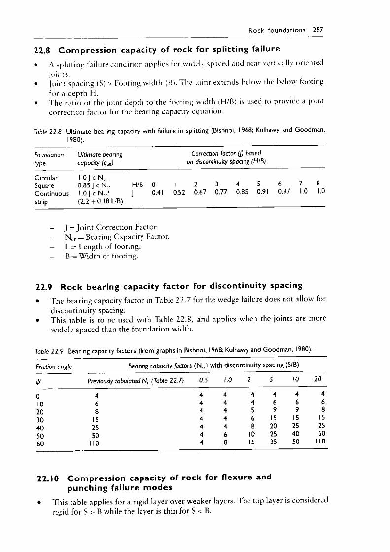
R o c k fo u n d a t ion s 287
22.8 C o m p ress io n capacity of rock for splitting failure• A splitting failure condition applies for widely spaced and near vertically oriented
joints.• Joint spacing (S) > Footing width (B). The joint extends below the below footing
for a depth H.• The ratio of the joint depth to the footing width (H/B) is used to provide a joint
correction factor for the bearing capacity equation.
Table 22.8 Ultimate bearing capacity with failure in splitting (Bishnoi, 1968; Kulhawy and Goodman,1980).
Foundationtype
Ultimate bearing capacity (qu,t)
Correction factor (J) based on discontinuity spacing (HIB)
CircularSquareContinuousstrip
1 0 J c N cr0.85 J c Ncr H/B 0 1.0 J c N cr/ J 0.41 (2.2 + 0.18 L/B)
1 2 3 4 5 6 7 8 0.52 0.67 0.77 0.85 0.91 0.97 1.0 1.0
- J = Jo in t Correction Factor.- Ncr = Bearing Capacity Factor.- L = Length of footing.
B = Width of footing.
22.9 R o ck bearing capacity factor for discontinuity spacing• The bearing capacity factor in Table 2 2 .7 for the wedge failure does not allow for
discontinuity spacing.• This table is to be used with Table 2 2 .8 , and applies when the joints are more
widely spaced than the foundation width.
Table 22.9 Bearing capacity factors (from graphs in Bishnoi, 1968; Kulhawy and Goodman, 1980).
Friction angle Bearing capacity factors (Ncr) with discontinuity spacing (S/B)
<P Previously tabulated Nc (Table 22.1) 0.5 1.0 2 5 10 20
0 4 4 4 4 4 4 410 6 4 4 4 6 6 620 8 4 4 5 9 9 830 15 4 4 6 15 15 1540 25 4 4 8 20 25 2550 50 4 6 10 25 40 5060 1 10 4 8 15 35 50 1 10
22.10 C o m p ress io n capacity of rock for flexure and punching failure modes
• This table applies for a rigid layer over weaker layers. The top layer is considered rigid for S > B while the layer is thin for S < B.
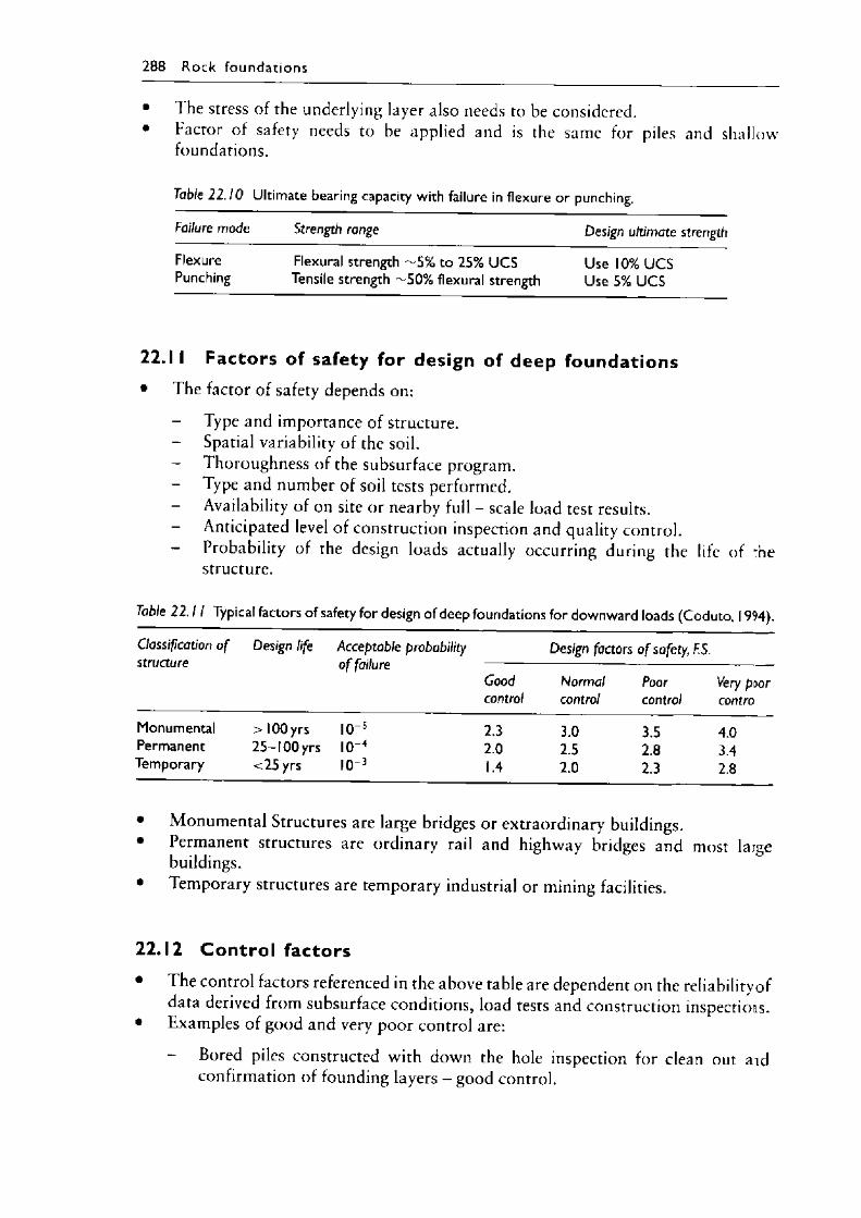
288 R o c k fo und a tio ns
• The stress of the underlying layer also needs to be considered.• Factor o f safety needs to be applied and is the same for piles and shallow
foundations.
Table 22.10 Ultimate bearing capacity with failure in flexure or punching.
Failure mode Strength range Design ultimate strength
Flexure Flexural strength ~5% to 25% UCS Use 10% UCSPunching Tensile strength ^50% flexural strength Use 5% U CS
22.1 I Factors of safety for design of deep foundations• The factor of safety depends on:
Type and importance of structure.- Spatial variability of the soil.- Thoroughness of the subsurface program.
Type and number of soil tests performed.- Availability of on site or nearby full - scale load test results.
Anticipated level of construction inspection and quality control.- Probability of the design loads actually occurring during the life of *he
structure.
Table 2 2 .1 1 Typical factors of safety for design of deep foundations for downward loads (Coduto, 1994).
Classification o f structure
Design life Acceptable probability o f failure
Design factors o f safety\ F.S.
Goodcontrol
Normalcontrol
Poorcontrol
Very poor contro
Monumental > 100 yrs 10 5 2.3 3.0 3.5 4.0Permanent 25-100 yrs 10 4 2.0 2.5 2.8 3.4Temporary <25 yrs 10 3 1.4 2.0 2.3 2.8
• Monumental Structures are large bridges or extraordinary buildings.• Permanent structures are ordinary rail and highway bridges and most large
buildings.• Temporary structures are temporary industrial or mining facilities.
22.12 C ontro l factors• The control factors referenced in the above table are dependent on the reliability of
data derived from subsurface conditions, load tests and construction inspections.• Examples of good and very poor control are:
- Bored piles constructed with down the hole inspection for clean out aid confirmation of founding layers - good control.
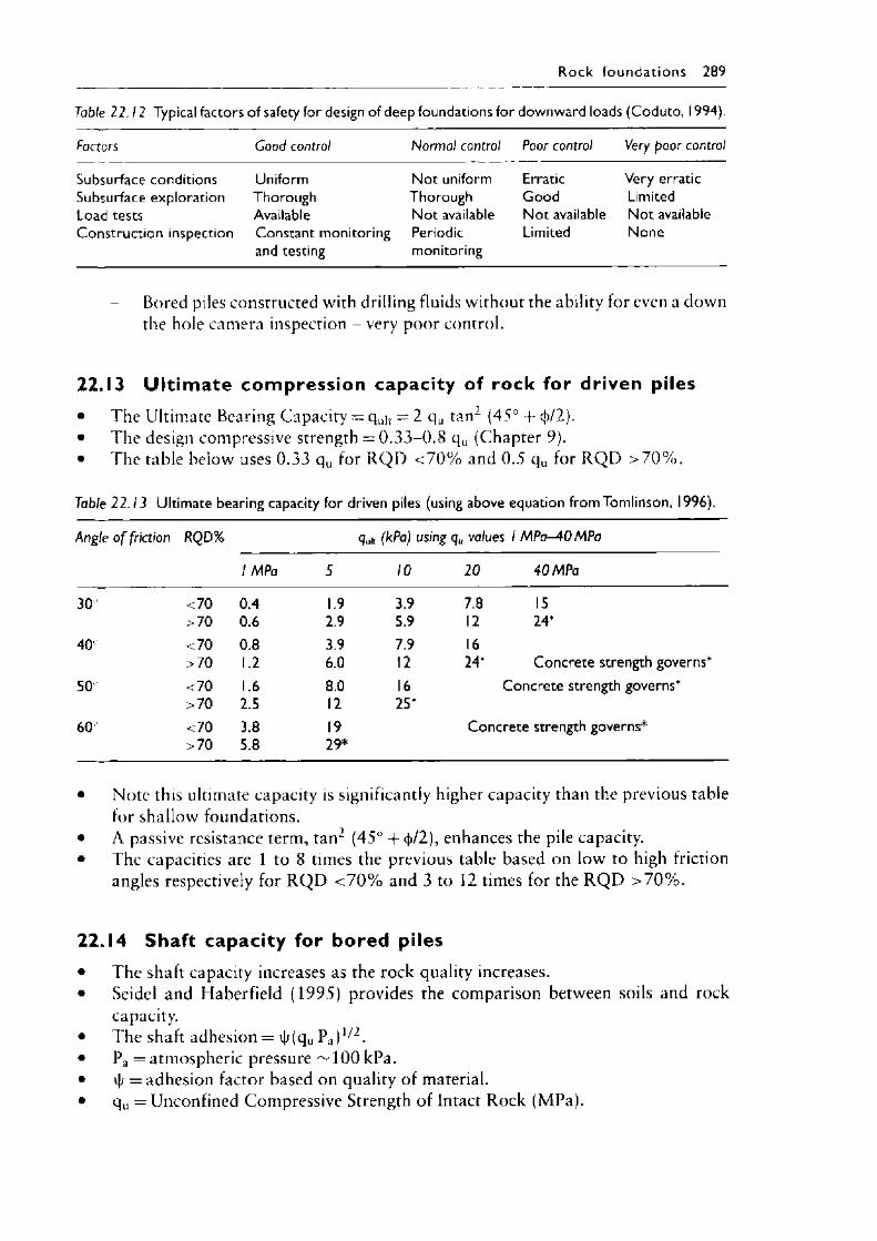
R o c k fo und a t io ns 289
Table 2 2 .12 Typical factors of safety for design of deep foundations for downward loads (Coduto, 1994).
Factors Good control Normal control Poor control Very poor control
Subsurface conditions Uniform Not uniform Erratic Very erraticSubsurface exploration Thorough Thorough Good LimitedLoad tests Available Not available Not available Not availableConstruction inspection Constant monitoring Periodic Limited None
and testing monitoring
- Bored piles constructed with drilling fluids without the ability for even a down the hole camera inspection - very poor control.
22.13 U lt im ate com press ion capacity of rock for driven piles• The Ultimate Bearing Capacity = q u|t = 2 qu tan2 (45° + cj>/2).• The design compressive strength = 0 . 3 3 - 0 . 8 qu (Chapter 9).• The table below uses 0 .33 qu for R Q D < 7 0 % and 0.5 qu for R Q D > 7 0 % .
Table 22.13 Ultimate bearing capacity for driven piles (using above equation from Tomlinson, 1996).
Angle o f friction RQD% quit (kPa) using qu values I M Pa-40 MPa
1 MPa 5 10 20 40 MPa
30 <70 0.4 1.9 3.9 7.8 15>70 0.6 2.9 5.9 12 24*
40 <70 0.8 3.9 7.9 16>70 1.2 6.0 12 24* Concrete strength governs*
50 <70 1.6 8.0 16 Concrete strength governs*>70 2.5 12 25*
60 <70 3.8 19 Concrete strength governs*>70 5.8 29*
• Note this ultimate capacity is significantly higher capacity than the previous table for shallow foundations.
• A passive resistance term, tan2 (45° + <j>/2), enhances the pile capacity.• The capacities are 1 to 8 times the previous table based on low to high friction
angles respectively for R Q D < 7 0 % and 3 to 12 times for the R Q D > 7 0 % .
22.14 Shaft capacity for bored piles• The shaft capacity increases as the rock quality increases.• Seidel and Haberfield (1995) provides the comparison between soils and rock
capacity.• The shaft adhesion = \J/(qu Pa)1/2.• pa = atmospheric pressure ^ 1 0 0 kPa.• v|/ = adhesion factor based on quality of material.• qu = Unconfined Compressive Strength of Intact Rock (MPa).
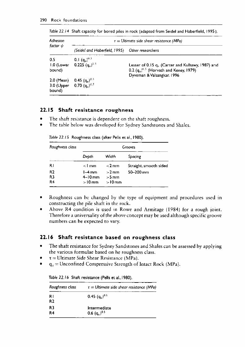
290 R o c k founda t ions
Table 22.14 Shaft capacity for bored piles in rock (adapted from Seidel and Haberfield, 1995 ).
Adhesion r = Ultimate side shear resistance (MPa)factor xjz ------------------------------------------------------------------------------
(Seidel and Haberfield, 1995) Other researchers
0.5 0.1 (qu)°51.0 (Lower 0.225 (qu)1'■' Lesser of 0.15 q„ (Carter and Kulhawy, 1 987) andbound) 0.2 (qu) ° 5 (Horvath and Keney, 1979)
Dyveman &Valsangkar, 19962.0 (Mean) 0.45 (qu) ° '3.0 (Upper 0.70 (qu)° 5bound)
22.15 Shaft res istance roughness• The shaft resistance is dependent on the shaft roughness.• The table below was developed for Sydney Sandstones and Shales.
Table 22.15 Roughness class (after Pells et al., 1980).
Roughness class Grooves
Depth Width Spacing
Rl < 1 mm <2 mm Straight, smooth sidedR2 1-4 mm >2 mm 50-200 mmR3 4-10 mm >5 mmR4 > 10 mm > 10 mm
• Roughness can be changed by the type of equipment and procedures used in constructing the pile shaft in the rock.
• Above R 4 condition is used in Rowe and Armitage (1984) for a rough joint. Therefore a universality of the above concept may be used although specific groove numbers can be expected to vary.
22.16 Shaft res istance based on roughness class• The shaft resistance for Sydney Sandstones and Shales can be assessed by applying
the various formulae based on he roughness class.• t = Ultimate Side Shear Resistance (MPa).• qu = Unconfined Compressive Strength of Intact Rock (MPa).
Table 22.16 Shaft resistance (Pells et al., 1980).
Roughness class r = Ultimate side shear resistance (MPa)
Rl 045 (qu)°5R2R3 IntermediateR4 0.6 (qu)05
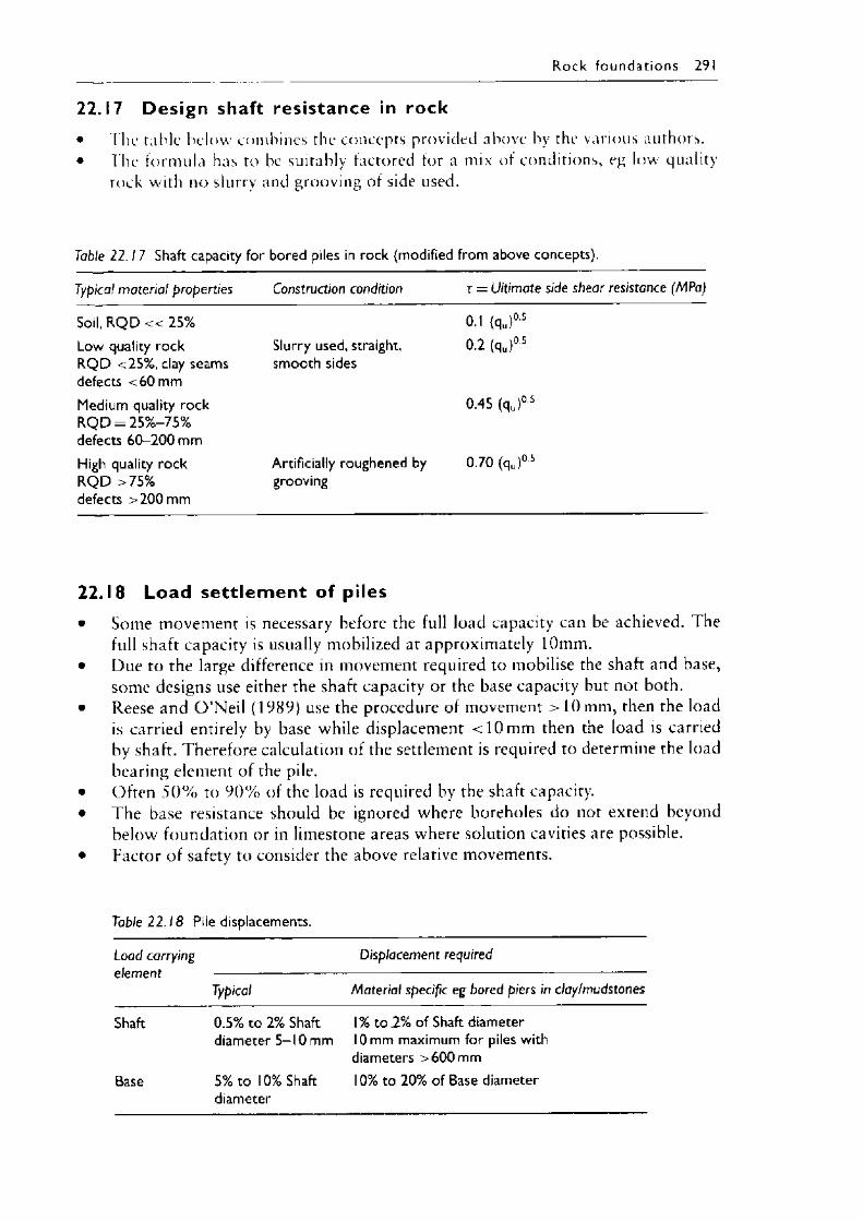
R o c k fo und a tions 291
22.17 Design shaft resistance in rock• The table below combines the concepts provided above by the various authors.• T he formula has to be suitably factored for a mix of conditions, eg low quality
rock with no slurry and grooving of side used.
Table 22.1 7 Shaft capacity for bored piles in rock (modified from above concepts).
Typical material properties Construction condition r = Ultimate side shear resistance (MPa)
Soil, R Q D « 25% 0.1 (qu)°5Low quality rock R Q D <25%, clay seams defects <60 mm
Slurry used, straight, smooth sides
0.2 (qu)°5
Medium quality rock R Q D = 25%-75% defects 60-200 mm
0.45 (qu)°5
High quality rock R Q D >75% defects >200 mm
Artificially roughened by grooving
0.70 ( q j05
22.18 Load sett lem ent of piles• Some movement is necessary before the full load capacity can be achieved. The
full shaft capacity is usually mobilized at approximately 10mm.• Due to the large difference in movement required to mobilise the shaft and base,
some designs use either the shaft capacity or the base capacity but not both.• Reese and O ’Neil (1989) use the procedure of movement > 10 mm, then the load
is carried entirely by base while displacement < 1 0 mm then the load is carried by shaft. Therefore calculation of the settlement is required to determine the load bearing element of the pile.
• Often 5 0 % to 9 0 % of the load is required by the shaft capacity.• The base resistance should be ignored where boreholes do not extend beyond
below foundation or in limestone areas where solution cavities are possible.F a c t o r o f sa fety to co n s id e r the ab o ve re lative m o vem en ts.
Table 22 .18 Pile displacements.
Load carrying element
Displacement required
Typical Material specific eg bored piers in clay/mudstones
Shaft 0.5% to 2% Shaft diameter 5-10 mm
1% to 2% of Shaft diameter 10 mm maximum for piles with diameters >600 mm
Base 5% to 10% Shaft diameter
10% to 20% of Base diameter
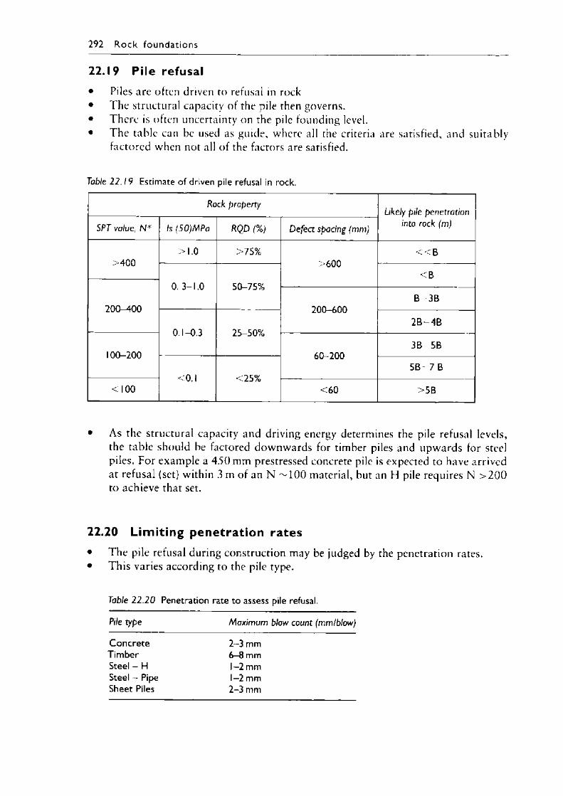
292 R o c k fo und a t io ns
22.19 Pile refusal• Piles are often driven to refusal in rock• The structural capacity of the pile then governs.• There is often uncertainty on the pile founding level.• The table can be used as guide, where all the criteria are satisfied, and suitably
factored when not all of the factors are satisfied.
Table 2 2 .19 Estimate of driven pile refusal in rock.
Rock propertyLikely pile penetration
into rock (m)SPT value, N * Is (SO)tAPa RQD (%) Defect spacing (mm)
>400
200-400
>1.0 >75%>600
< < B
0. 3-1.0 50-75%< B
200-600B - 3 B
0.1-0.3 25-50%2B 4B
100-200 60-2003B 5B
<0.1 <25%5B 7 B
<100 <60 >5B
As the structural capacity and driving energy determines the pile refusal levels, the table should be factored downwards for timber piles and upwards for steel piles. For example a 4 5 0 mm prestressed concrete pile is expected to have arrived at refusal (set) within 3 m of an N -TOO material, but an FJ pile requires N > 2 0 0 to achieve that set.
22.20 L im it ing penetrat ion rates• The pile refusal during construction may be judged by the penetration rates.• This varies according to the pile type.
Table 22 .20 Penetration rate to assess pile refusal.
Pile type Maximum blow count (mm/blow)
Concrete 2-3 mmTimber 6-8 mmSteel - H 1-2 mmSteel - Pipe 1-2 mmSheet Piles 2-3 mm
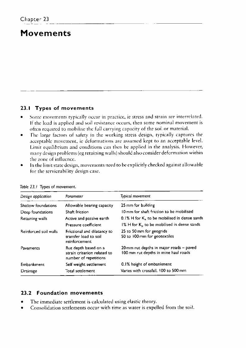
MovementsChapter 23
23.1 Types of m ovem ents• Some movements typically occur in practice, ie stress and strain are interrelated.
If the load is applied and soil resistance occurs, then some nominal movement is often required to mobilise the full carrying capacity of the soil or material.
• The large factors of safety in the working stress design, typically captures the acceptable movement, ie deformations are assumed kept to an acceptable level. Limit equilibrium and conditions can then be applied in the analysis. However, many design problems (eg retaining walls) should also consider deformation within the zone of influence.
• In the limit state design, movements need to be explicitly checked against allowable for the serviceability design case.
Table 2 3 .1 Types of movement.
Design application Parameter Typical movement
Shallow foundations Deep foundations Retaining walls
Reinforced soil walls
Pavements
EmbankmentDrainage
Allowable bearing capacityShaft frictionActive and passive earthPressure coefficientFrictional and dilatancy to transfer load to soil reinforcementRut depth based on a strain criterion related to number of repetitionsSelf weight settlementTotal settlement
25 mm for buildingI Omm for shaft friction to be mobilised0.1% H for Ka to be mobilised in dense sands1% H for Kp to be mobilised in dense sands25 to 50 mm for geogrids 50 to 100 mm for geotextiles
20 mm rut depths in major roads - paved 100 mm rut depths in mine haul roads
0 .1 % height of embankment Varies with crossfall. 100 to 500 mm
23.2 Foundation m ovem ents• The immediate settlement is calculated using elastic theory.• Consolidation settlements occur with time as water is expelled from the soil.
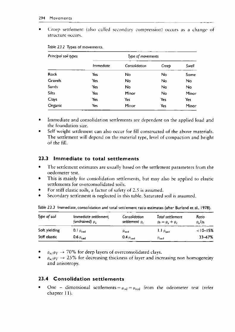
294 M o vem en ts
Creep settlement (also called secondary compression) occurs as a change of structure occurs.
Table 23.2 Types of movements.
Principal soil types Type o f movements
Immediate Consolidation Creep Swell
Rock Yes No No SomeGravels Yes No No NoSands Yes No No NoSilts Yes Minor No MinorClays Yes Yes Yes YesOrganic Yes Minor Yes Minor
• Immediate and consolidation settlements are dependent on the applied load and the foundation size.
• Self weight settlement can also occur for fill constructed of the above materials.The settlement will depend on the material type, level of compaction and heighto f the fill.
23.3 Im m ediate to total sett lem ents• The settlement estimates are usually based on the settlement parameters from the
oedometer test.• This is mainly for consolidation settlements, but may also be applied to elastic
settlements for overconsolidated soils.• For stiff elastic soils, a factor of safety of 2.5 is assumed.• Secondary settlement is neglected in this table. Saturated soil is assumed.
Table 23.3 Immediate, consolidation and total settlement ratio estimates (after Burland et al., 1978).
Type o f soil Immediate settlement, Consolidation Total settlement Ratio(undrained) pu settlement pc Pr = Pu + Pc pjpr
Soft yielding °- 1 Poed Poed 1 •1 Poed <10-15%Stiff elastic 0-6 Poed 0-4 Poed Poed 33-67%
• Ph/Pt * 7 0 % for deep layers of overconsolidated clays.• P«/P7 ~> 2 5 % for decreasing thickness of iayer and increasing non homogeneity
and anisotropy.
23.4 Consolidation sett lem ents• One - dimensional settlements = potj = poetj from the odeometer test (refer
chapter 11).
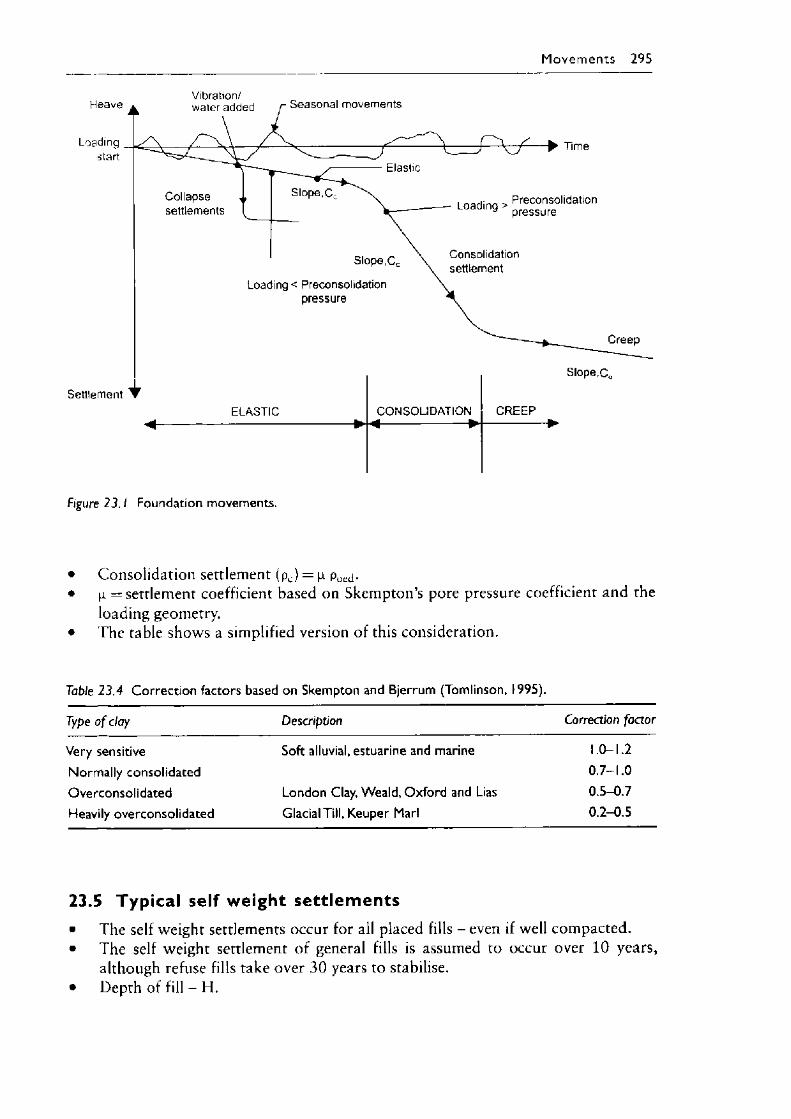
M ovem en ts 295
Vibration/
Figure 2 3 .1 Foundation movements.
• Consolidation settlement (pc ) = \i poe£j .• \x = settlement coefficient based on Skempton’s pore pressure coefficient and the
loading geometry.• The table shows a simplified version of this consideration.
Table 23.4 Correction factors based on Skempton and Bjerrum (Tomlinson, 1995).
Type o f clay Description Correction factor
Very sensitive Soft alluvial, estuarine and marine 1.0-1.2Normally consolidated 0.7-1.0Overconsolidated London Clay, Weald, Oxford and Lias 0.5-0.7Heavily overconsolidated Glacial Till, Keuper Marl 0.2-0.5
23.5 T y p ic a l se lf w e igh t s e t t l e m e n t s• The self weight settlements occur for all placed fills - even if well compacted.• The self weight settlement of general fills is assumed to occur over 10 years,
although refuse fills take over 30 years to stabilise.• Depth of fill - H.
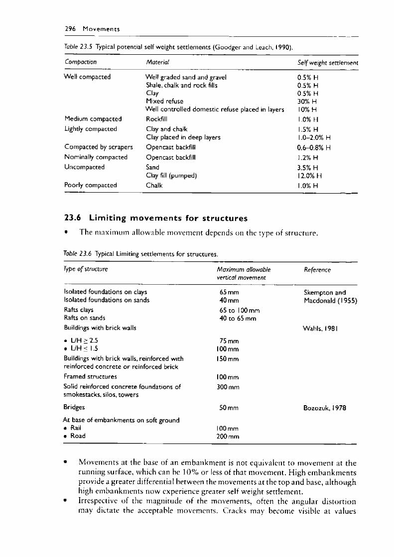
296 M ovem ents
Table 23.5 Typical potential self weight settlements (Goodger and Leach, 1990).
Compaction Material Se lf weight settlement
Well compacted Well graded sand and gravel 0.5% HShale, chalk and rock fills 0.5% HClay 0.5% HMixed refuse 30% HWell controlled domestic refuse placed in layers 10% H
Medium compacted Rockfill 1.0% HLightly compacted Clay and chalk 1.5% H
Clay placed in deep layers 1.0-2.0% HCompacted by scrapers Opencast backfill 0.6-0.8% HNominally compacted Opencast backfill 1.2% HUncompacted Sand 3.5% H
Clay fill (pumped) 12.0% HPoorly compacted Chalk 1.0% H
23.6 L im it in g m o v e m e n t s for s t ru c tu re s• The maximum allowable movement depends on the type of structure.
Table 23.6 Typical Limiting settlements for structures.
Type o f structure Maximum allowable vertical movement
Reference
Isolated foundations on clays Isolated foundations on sands
65 mm 40 mm
Skempton and Macdonald (1955)
Rafts clays Rafts on sands
65 to 100 mm 40 to 65 mm
Buildings with brick walls Wahls, 1981• U H > 2.5• UH < 1.5
75 mm 100 mm
Buildings with brick walls, reinforced with reinforced concrete or reinforced brick
150 mm
Framed structures 100 mmSolid reinforced concrete foundations of smokestacks, silos, towers
300 mm
Bridges 50 mm Bozozuk, 1978At base of embankments on soft ground• Rail• Road
100 mm 200 mm
Movements at the base of an embankment is not equivalent to movement at the running surface, which can be 1 0 % or less of that movement. High embankments provide a greater differential between the movements at the top and base, although high embankments now experience greater self weight settlement.Irrespective of the magnitude of the movements, often the angular distortion may dictate the acceptable movements. Cracks may become visible at values
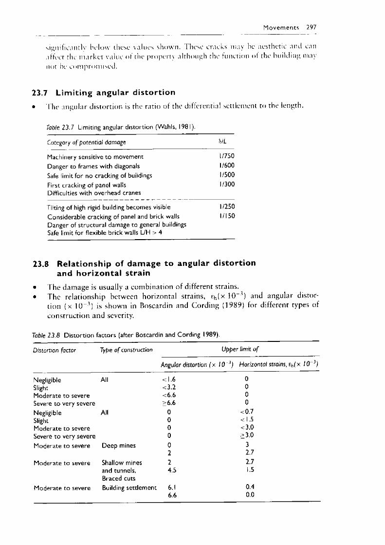
significantly below these values shown. These cracks may be aesthetic and can affect the market value of the property although the function of the building may not be compromised.
23.7 L im it in g ang u la r d is tort ion• The angular distortion is the ratio of the differential settlement to the length.
M ovem ents 297
Table 23.7 Limiting angular distortion (Wahls, 1981).
Category o f potential damage h/L
Machinery sensitive to movement 1/750Danger to frames with diagonals 1/600Safe limit for no cracking of buildings 1/500First cracking of panel walls Difficulties with overhead cranes
1/300
Tilting of high rigid building becomes visible 1/250Considerable cracking of panel and brick walls Danger of structural damage to general buildings Safe limit for flexible brick walls L/H > 4
1/150
23.8 R e la t io n sh ip of d a m a g e to angular d istort ion and h o r iz o n ta l stra in
• The damage is usually a combination of different strains.• The relationship between horizontal strains, 1 0 ^ ) and angular distor
tion (x 10~3) is shown in Boscardin and Cording (1989) for different types of construction and severity.
Table 23.8 Distortion factors (after Boscardin and Cording 1989).
Distortion factor Type o f construction Upper limit o f
Angular distortion ( x 10 3) Horizontal strains, eh( x 10 3)
Negligible All < 1.6 0Slight <3.2 0Moderate to severe <6.6 0Severe to very severe >6.6 0Negligible All 0 <0.7Slight 0 <1.5Moderate to severe 0 <3.0Severe to very severe 0 >3.0Moderate to severe Deep mines 0 3
2 2.7Moderate to severe Shallow mines 2 2.7
and tunnels, 4.5 1.5Braced cuts
Moderate to severe Building settlement 6.1 0.46.6 0.0
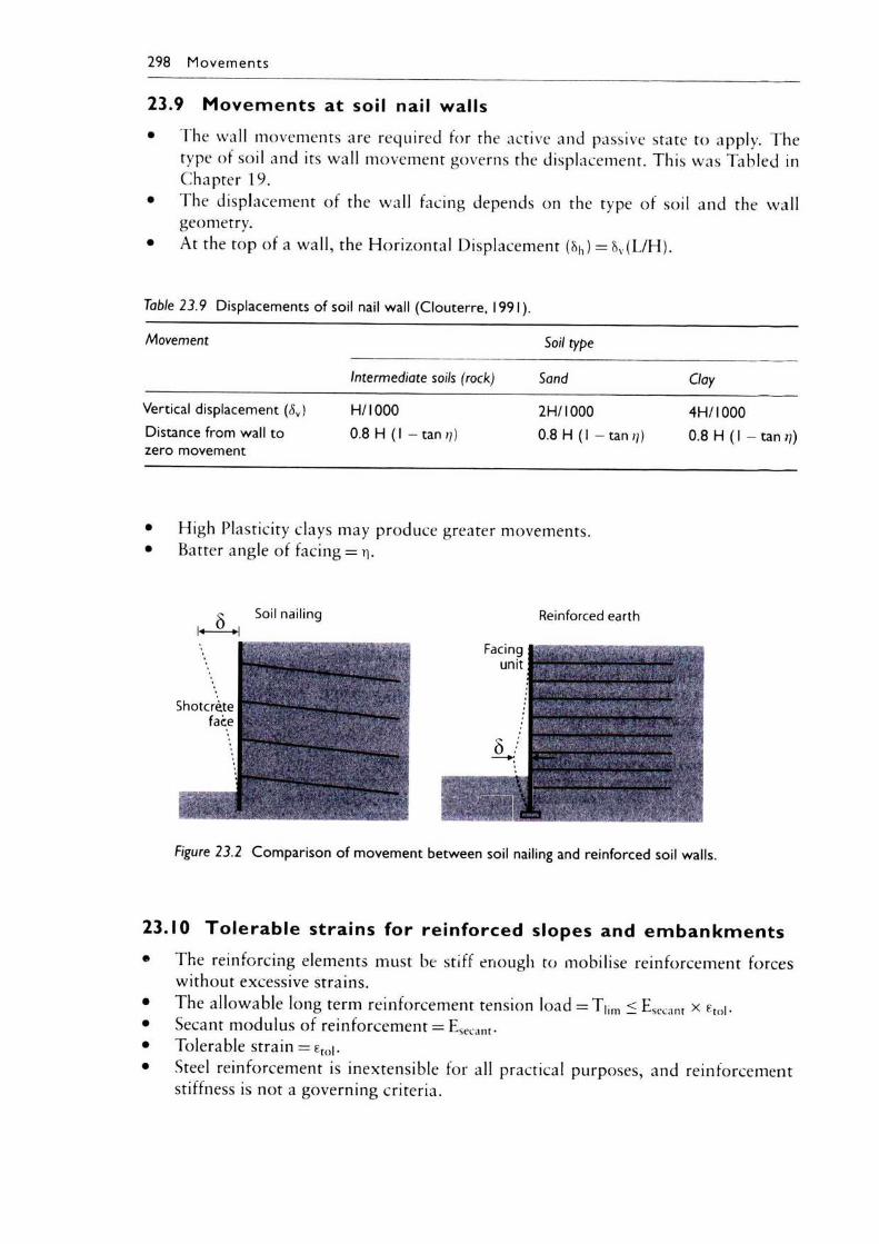
298 M ovem ents
23.9 M o v e m e n ts at soil nail walls• The wall movements are required for the active and passive state to apply. The
type of soil and its wall movement governs the displacement. This was Tabled in Chapter 19.
• The displacement of the wall facing depends on the type of soil and the wall geometry.
• At the top of a wall, the Horizontal Displacement (&h) = 8V(L/H).
Table 23.9 Displacements of soil nail wall (Clouterre, 1991).
Movement Soil type
Intermediate soils (rock) Sand Clay
Vertical displacement (5V) H/1000 2H/I000 4H/I000Distance from wall to 0.8 H ( 1 — tan rj) 0.8 H (1 — tan //) 0.8 H (1 — tan rj)zero movement
• High Plasticity clays may produce greater movements.• Batter angle of facing = r\.
Soil nailing Reinforced earth
Facingunit
p a ? ........... ;.p *
Figure 23.2 Comparison of movement between soil nailing and reinforced soil walls.
23.10 T o le r a b le s t ra in s for re in forced slopes and e m b a n k m e n t s• The reinforcing elements must be stiff enough to mobilise reinforcement forces
without excessive strains.• The allowable long term reinforcement tension load = T|im < EseCant x etoi-• Secant modulus of reinforcement = Esecanf• Tolerable strain = 8to|.• Steel reinforcement is inextensible for all practical purposes, and reinforcement
stiffness is not a governing criteria.
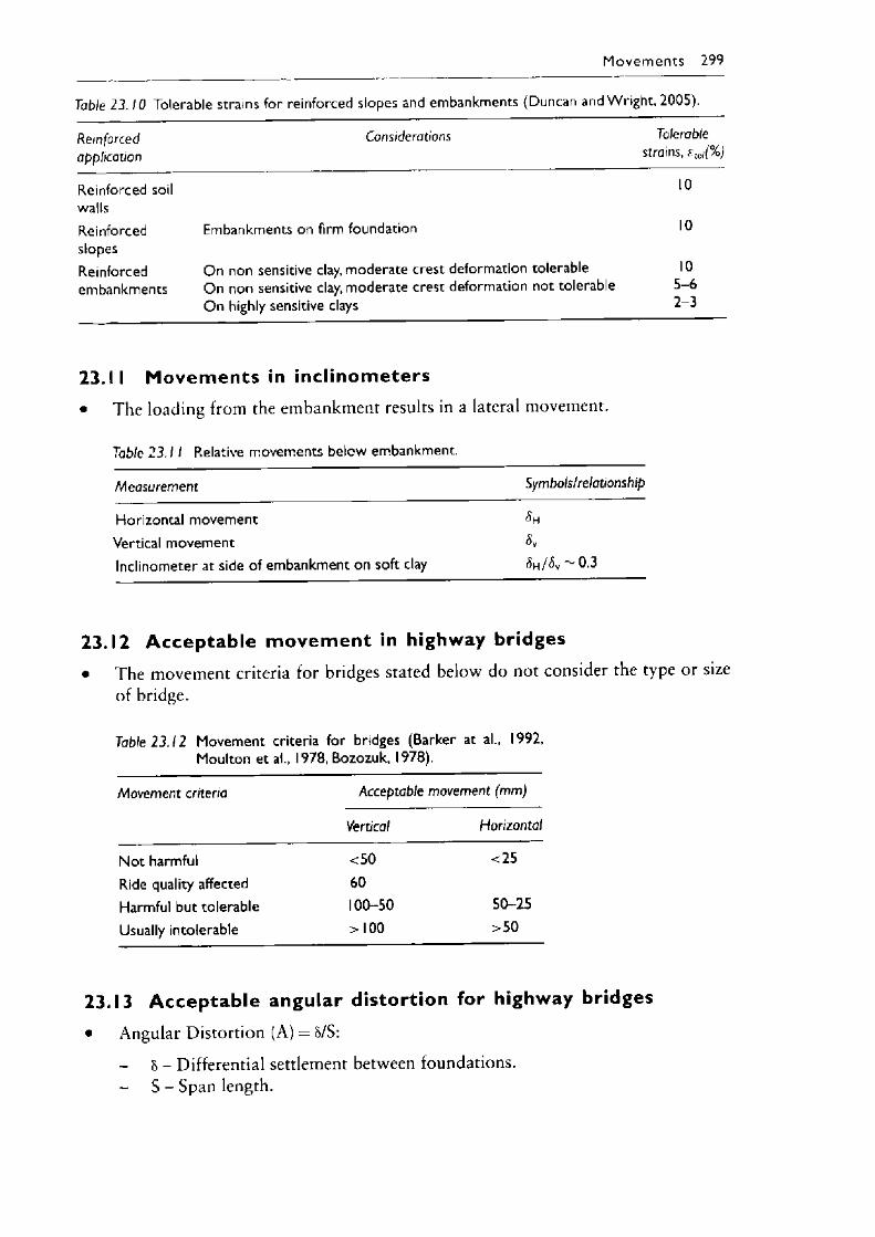
M ovem en ts 299
Table 23.10 Tolerable strains for reinforced slopes and embankments (Duncan and Wright, 2005).
Reinforcedapplication
Considerations Tolerable strains, f toi(%)
Reinforced soil 10wallsReinforced Embankments on firm foundation 10slopesReinforced On non sensitive clay, moderate crest deformation tolerable 10embankments On non sensitive clay, moderate crest deformation not tolerable 5-6
On highly sensitive clays 2-3
23.11 M o v e m e n ts in in c l in o m e te r s• The loading from the embankment results in a lateral movement.
Tabic 23.11 Relative movements below embankment.
Measurement Symbols! relationship
Horizontal movement 5h
Vertical movement SvInclinometer at side of embankment on soft clay W<$v~0.3
23.12 A c c e p t a b le m o v e m e n t in h ighway br idges• The movement criteria for bridges stated below do not consider the type or size
of bridge.
Table 2 3 .12 Movement criteria for bridges (Barker at al., 1992, Moulton et al., 1978, Bozozuk, 1978).
Movement criteria Acceptable movement (mm)
Vertical Horizontal
Not harmful <50 <25Ride quality affected 60Harmful but tolerable 100-50 50-25Usually intolerable >100 >50
23.13 A c c e p t a b le ang u la r d is to rt io n for h ighway bridges• Angular Distortion (A) = 8/S:
h - Differential settlement between foundations.S - Span length.
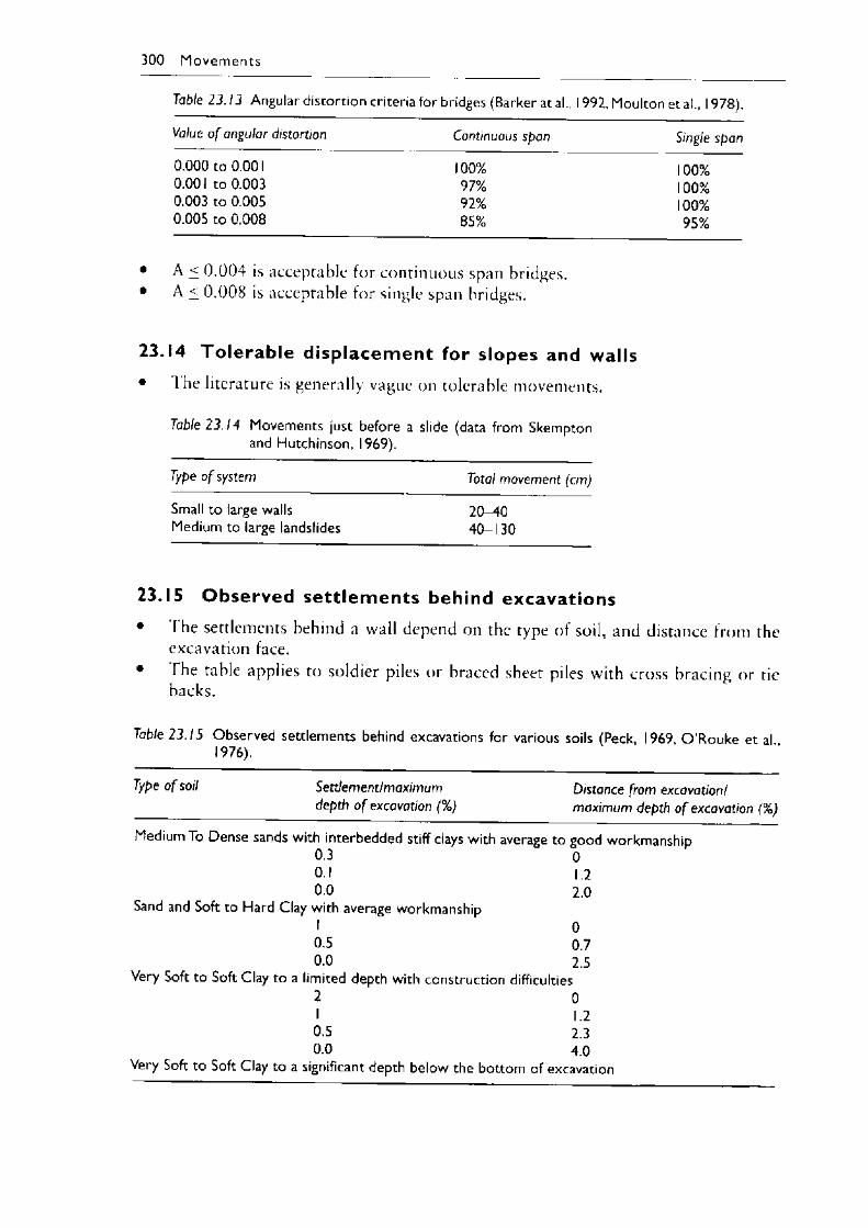
300 M ovem ents
Table 23.13 Angular distortion criteria for bridges (Barker at al., 1992, Moulton et al., 1978).
Value o f angular distortion Continuous span Single span
0.000 to 0.001 100% 100%0.001 to 0.003 97% 100%0.003 to 0.005 92% 100%0.005 to 0.008 85% 95%
• A < 0 .004 is acceptable for continuous span bridges.• A < 0 .008 is acceptable for single span bridges.
23.14 T o le ra b le d i s p la c e m e n t for s lopes and walls• The literature is generally vague on tolerable movements.
Table 2 3 .14 Movements just before a slide (data from Skempton and Hutchinson, 1969).
Type o f system Total movement (cm)
Small to large walls 20-^0Medium to large landslides 40-130
23.15 O b s e r v e d s e t t l e m e n t s behind ex cav at io n s• The settlements behind a wall depend on the type of soil, and distance from the
excavation face.• The table applies to soldier piles or braced sheet piles with cross bracing or tie
backs.
Table 23.15 Observed settlements behind excavations for various soils (Peck, 1969, O ’Rouke et al 1976).
Type o f soil Settlement/maximum Distance from excavation/depth o f excavation (%) maximum depth o f excavation (%)
Medium To Dense sands with interbedded stiff clays with average to good workmanship0.3 00.1 1.20.0 2.0
Sand and Soft to Hard Clay with average workmanship1 00.5 0.70.0 2.5
Very Soft to Soft Clay to a limited depth with construction difficulties2 0I 1.20.5 2.30.0 4.0
Very Soft to Soft Clay to a significant depth below the bottom of excavation
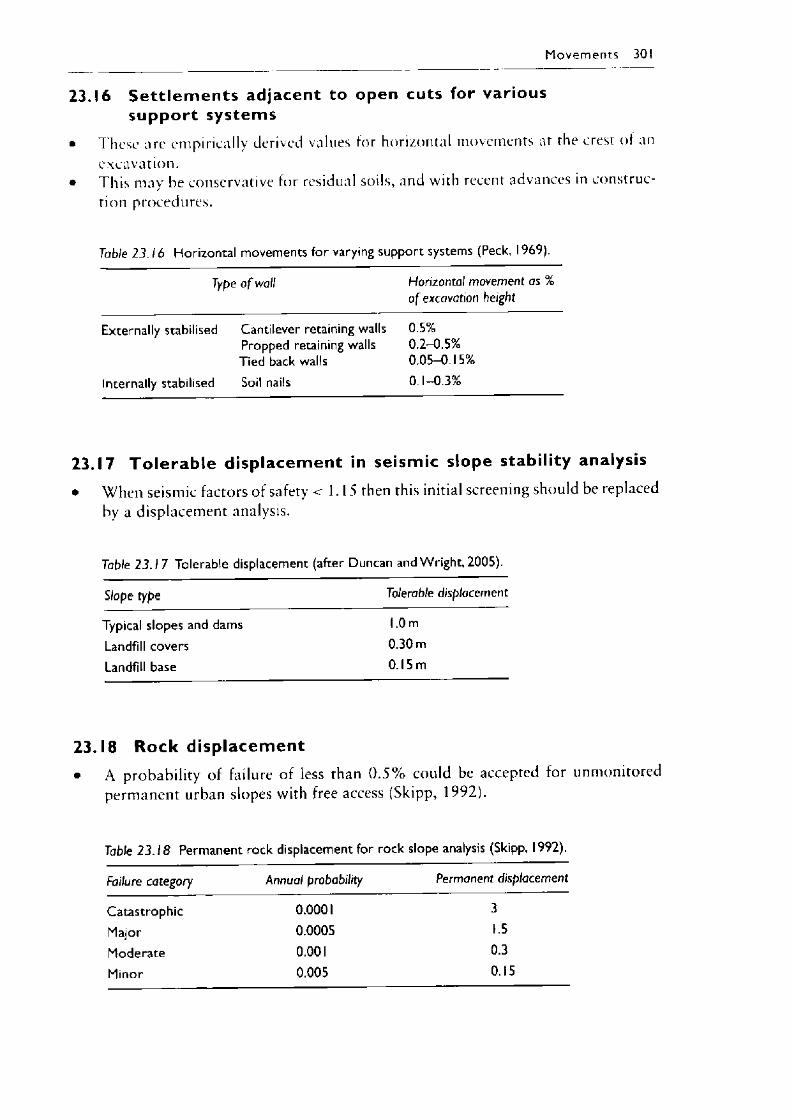
23.16 S e t t lem en ts adjacent to open cuts for various support systems
• These are empirically derived values for horizontal movements at the crest of an excavation.
• This may be conservative for residual soils, and with recent advances in construction procedures.
M ovem ents 301
Table 23.16 Horizontal movements for varying support systems (Peck, 1969).
Type o f wall Horizontal movement as %o f excavation height
Externally stabilised Cantilever retaining walls 0.5%Propped retaining walls 0.2-0.5%Tied back walls 0.05-0.15%
Internally stabilised Soil nails 0.1-0.3%
23.17 T o le rab le d isp lacement in se ismic slope stability analysis• When seismic factors of safety < 1.15 then this initial screening should be replaced
by a displacement analysis.
Table 23.1 7 Tolerable displacement (after Duncan and Wright, 2005).
Slope type Tolerable displacement
Typical slopes and dams 1.0 mLandfill covers 0.30 mLandfill base 0.15m
23.18 Ro ck d isp lacement• A probability of failure of less than 0 . 5 % could be accepted for unmonitored
permanent urban slopes with free access (Skipp, 1992).
Table 23 .18 Permanent rock displacement for rock slope analysis (Skipp, 1992).
Failure category Annual probability Permanent displacement
Catastrophic 0.0001 3Major 0.0005 1.5Moderate 0.001 0.3Minor 0.005 0.15
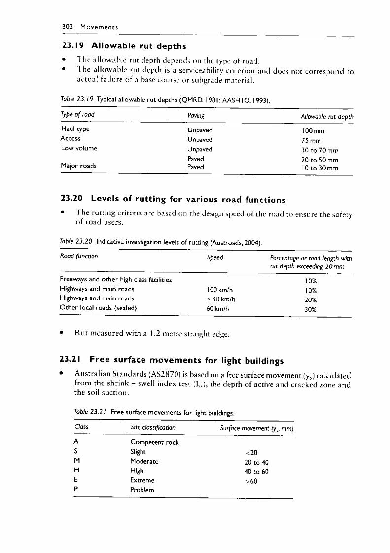
23.19 A l low ab le rut depths• 1 he allowable rut depth depends on the type of road.• The allowable rut depth is a serviceability criterion and does not correspond to
actual failure of a base course or subgrade material.
Table 23 .19 Typical allowable rut depths (QMRD, 1981: AASHTO, 1993).
Type o f road Paving Allowable rut depth
302 M o v e m e n ts
Haul type Unpaved 100 mmAccess Un paved 75 mmLow volume Unpaved 30 to 70 mm
Paved 20 to 50 mmMajor roads Paved 10 to 30 mm
23.20 Leve ls of rutting for various road functions• 1 he rutting criteria are based on the design speed of the road to ensure the safety
o f road users.
Table 23 .20 Indicative investigation levels of rutting (Austroads, 2004).
Road function Speed Percentage or road length withrut depth exceeding 20 mm
Freeways and other high class facilities Highways and main roads 100 km/h Highways and main roads <80 km/h O ther local roads (sealed) 60 km/h
10%10%20%30%
• Rut measured with a 1.2 metre straight edge.
23.21 F re e surface m ovem en ts for light buildings• Australian Standards (AS2870) is based on a free surface movement (ys) calculated
from the shrink - swell index test (Iss), the depth of active and cracked zone and the soil suction.
Table 23.21 Free surface movements for light buildings.
Class Site classification Surface movement (ys, mm)
A Competent rockS Slight <20M Moderate 20 to 40H High 40 to 60E Extreme >60P Problem
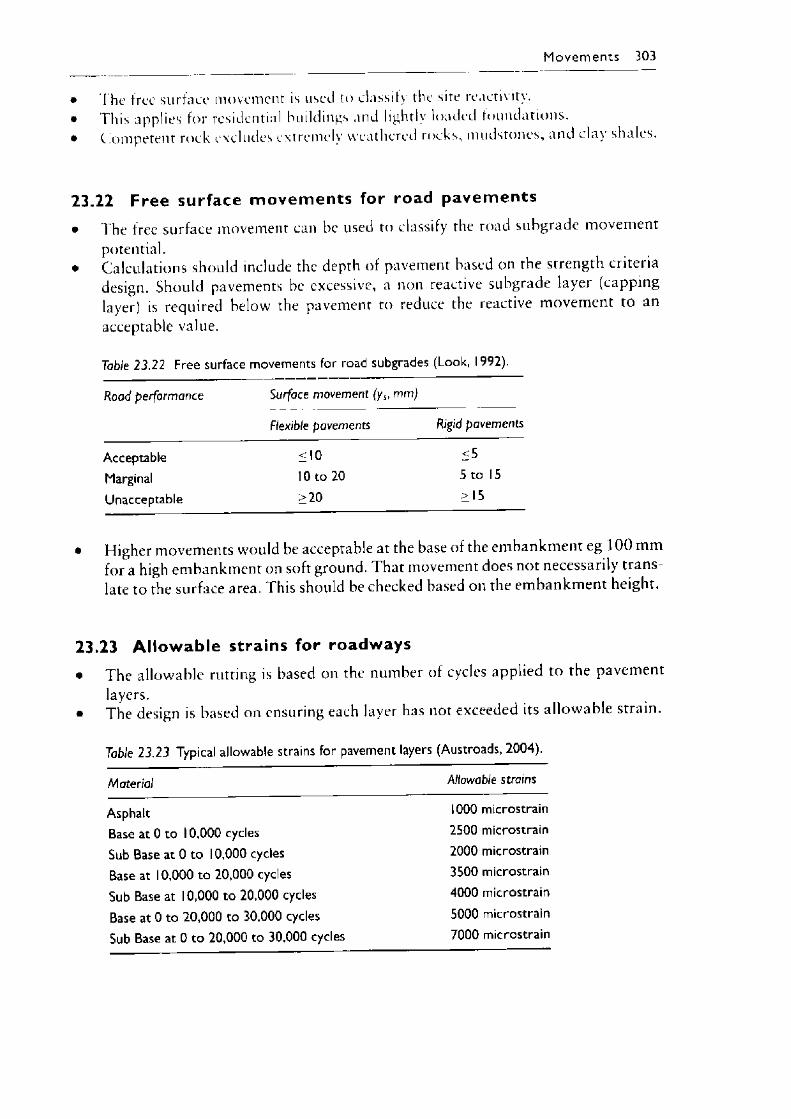
M o v e m e n ts 303
• The free surface movement is used to classify the site reactivity.• This applies for residential buildings and lightly loaded foundations.• Competent rock excludes extremely weathered rocks, mudstones, and clay shales.
23.22 Free surface m ovem ents for road pavements• The free surface movement can be used to classify the road subgrade movement
potential.• Calculations should include the depth of pavement based on the strength criteria
design. Should pavements be excessive, a non reactive subgrade layer (capping layer) is required below the pavement to reduce the reactive movement to an acceptable value.
Table 23.22 Free surface movements for road subgrades (Look, 1992).
Road performance Surface movement (ys, mm)
Flexible pavements Rigid pavements
Acceptable <10 <5
Marginal 10 to 20 5 to 15
Unacceptable >20 >15
• Higher movements would be acceptable at the base of the embankment eg 100 mm for a high embankment on soft ground. That movement does not necessarily translate to the surface area. This should be checked based on the embankment height.
23.23 A llowable strains for roadways• The allowable rutting is based on the number of cycles applied to the pavement
layers.• The design is based on ensuring each layer has not exceeded its allowable strain.
Table 23.23 Typical allowable strains for pavement layers (Austroads, 2004).
Material Allowable strains
Asphalt 1000 microstrainBase at 0 to 10,000 cycles 2500 microstrainSub Base at 0 to 10,000 cycles 2000 microstrainBase at 10,000 to 20,000 cycles 3500 microstrain
Sub Base at 10,000 to 20,000 cycles 4000 microstrain
Base at 0 to 20,000 to 30,000 cycles 5000 microstrainSub Base at 0 to 20,000 to 30,000 cycles 7000 microstrain

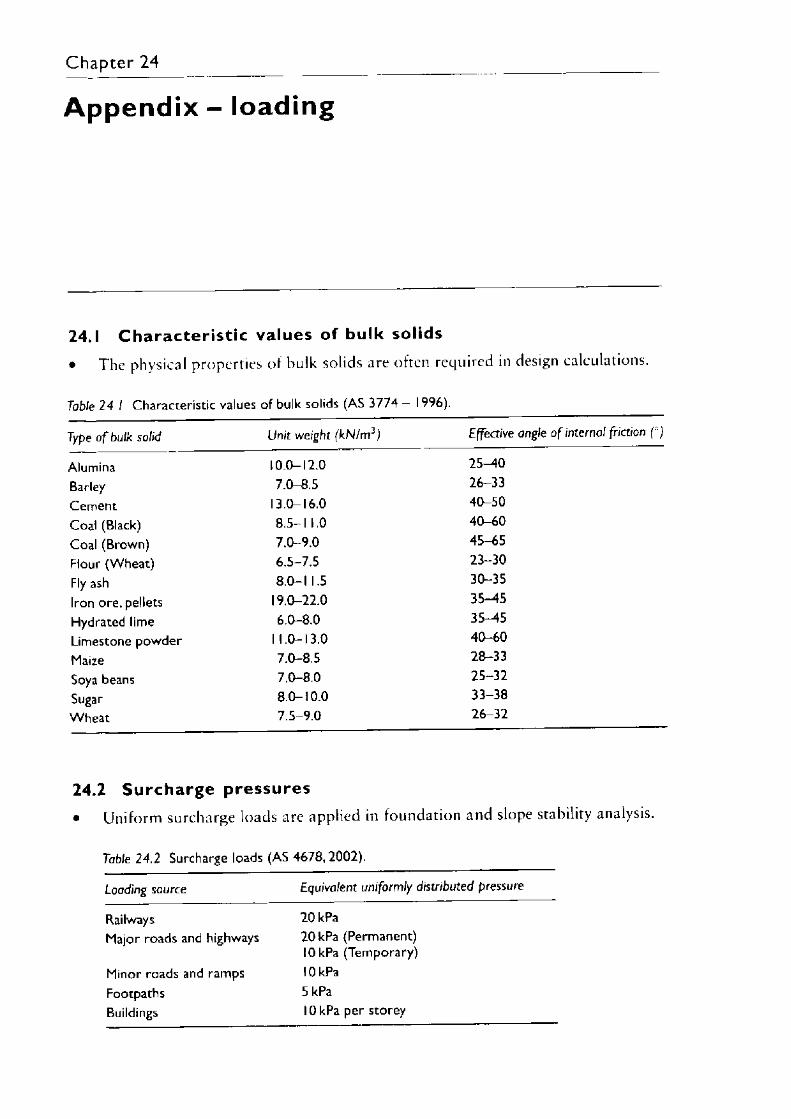
Chapter 24
Appendix - loading
24.1 C h a ra c t e r i s t i c values of bulk solids• The physical properties of hulk solids are often required in design calculations.
Table 24 I Characteristic values of bulk solids (AS 3774 - 1996).
Type o f bulk solid Unit weight (kN/m3) Effective angle o f internal friction (°)
Alumina 10.0-12.0 25-40Barley 7.0-8.5 26-33Cement 13.0-16.0 40-50Coal (Black) 8.5-1 1.0 40-60Coal (Brown) 7.0-9.0 45-65Flour (Wheat) 6.5-7.5 23-30Fly ash 8.0-1 1.5 30-35Iron ore, pellets 19.0-22.0 35-45Hydrated lime 6.0-8.0 35—45Limestone powder 1 1.0-13.0 40-60Maize 7.0-8.5 28-33Soya beans 7.0-8.0 25-32Sugar 8.0-10.0 33-38W heat 7.5-9.0 26-32
24.2 S u rcharg e pressures• Uniform surcharge loads are applied in foundation and slope stability analysis.
Table 24.2 Surcharge loads (AS 4678, 2002).
Loading source Equivalent uniformly distributed pressure
Railways 20 kPaMajor roads and highways 20 kPa (Permanent)
10 kPa (Temporary)Minor roads and ramps lOkPaFootpaths 5 kPaBuildings 10 kPa per storey
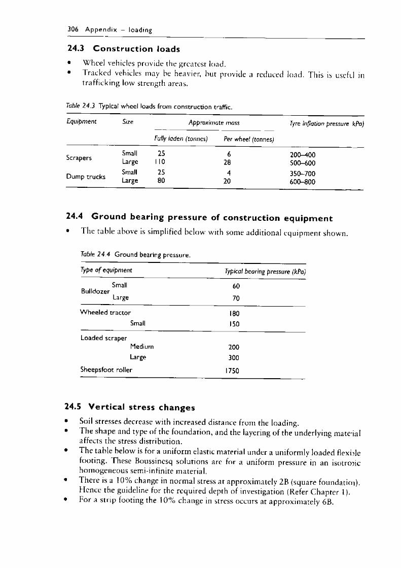
306 A p p e n d ix — loading
24.3 C onstru ct io n loads• Wheel vehicles provide the greatest load.• Tracked vehicles may be heavier, but provide a reduced
trafficking low strength areas.load. This is usefil in
Table 24.3 Typical wheel loads from construction traffic.
Equipment Size Approximate mass Tyre inflation pressure kPa)
Fully laden (tonnes) Per wheel (tonnes)
_ Small Scrapers ,r Largep. . Small Dump trucks Large
25 6 1 10 2825 4 80 20
200-400500-600350-700600-800
24.4 G ro un d bearing pressure of construction equipment• The table above is simplified below with some additional equipment shown.
Table 24 .4 Ground bearing pressure.
Type o f equipment Typical bearing pressure (kPa)
Small 60Bulldozer
Large 70
W heeled tractor 180Small 150
Loaded scraperMedium 200Large 300
Sheepsfoot roller 1750
24.5 V e rt ica l stress changes• Soil stresses decrease with increased distance from the loading.• The shape and type of the foundation, and the layering of the underlying mate’ial
affects the stress distribution.• The table below is for a uniform elastic material under a uniformly loaded flexible
footing. These Boussinesq solutions are for a uniform pressure in an isotropic homogeneous semi-infinite material.
• There is a 10% change in normal stress at approximately 2B (square foundatioi). Hence the guideline for the required depth of investigation (Refer Chapter 1).
• For a strip footing the 1 0 % change in stress occurs at approximately 6B.
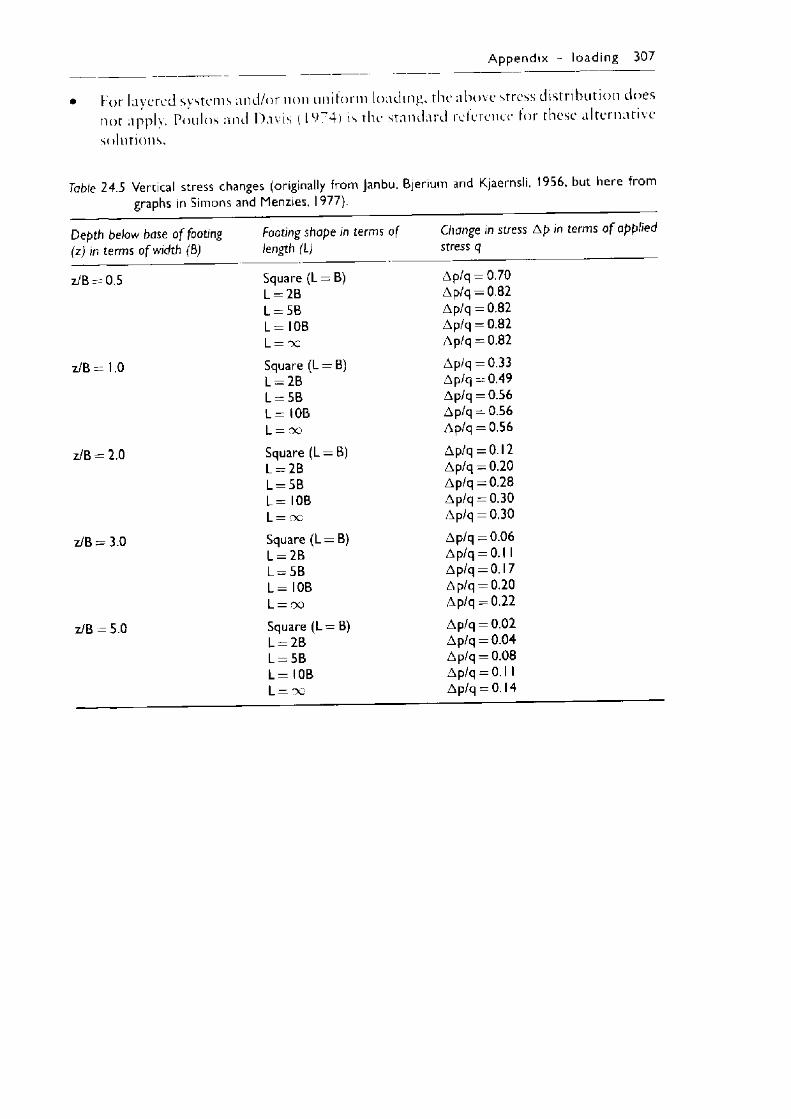
A ppen d ix - loading 307
• For layered systems and/or non uniform loading, the above stress distribution does not apply. Poulos and Davis (1974) is the standard reference for these alternative solutions.
Table 24.5 Vertical stress changes (originally from Janbu, Bjerium and Kjaernsli, 1956, but here from
Depth below base o f footing (z j in terms o f width (B)
Footing shape in terms o f length (L)
Change in stress A p in terms o f applied stress q
z/B = 0.5 Square (L = B) Ap/q = 0.70L = 2B Ap/q = 0.82L = 5B Ap/q = 0.82L = I0B Ap/q = 0.82L = oc Ap/q = 0.82
z/B = 1.0 Square (L = B) Ap/q = 0.33L = 2B Ap/q — 0.49L = 5B Ap/q = 0.56L = I0B Ap/q = 0.56L = oo Ap/q = 0.56
z/B = 2.0 Square (L = B) Ap/q = 0.12L = 2B Ap/q = 0.20L = 5B Ap/q = 0.28L = I0B Ap/q = 0.30L = oo Ap/q = 0.30
z/B = 3.0 Square (L = B) Ap/q = 0.06L = 2B Ap/q = 0.1 1L = 5 B Ap/q = 0.17L = I0B Ap/q = 0.20L = oo Ap/q = 0.22
z/B = 5.0 Square (L = B) Ap/q = 0.02L = 2B Ap/q = 0.04L = 5B Ap/q = 0.08L = I0B Ap/q = 0.11L = oo Ap/q = 0.14

Chapter 25
References
• References have been tabulated as essential background (General) to understanding the background of the data tables provided.
• References specific to whether investigations and assessment, or analysis anddesign. The references in the latter may not be repeated if already in investigations and assessments
25.1 G en e ra l - m o st used• Barnes G.E. ( 2 0 0 0 ) “ Soil Mechanics - Principles and Practice” 2nd Edition
Macmillan Press.• Barker R .M . , Duncan J . M . , Roj iani K.N., Ooi P.S.K., Tan C.K. and Kim S.G.
(1991 ) , “ Manuals for the design o f bridge foundations” National Cooperative Highway Research Program Report No 3 4 3 , Transportation Research Board, Washington.
• Bowles J .E . (1996 ) , “ Foundation Analysis and Design” 5th Edition M c g ra w -H i l l .• Carter M. (1 9 8 3 ) , “ Geotechnical Engineering Handbook” Pentech Press.• Das B.M. (1 9 9 9 ) , “ Principles of Foundation Engineering” 4th Edition,
Brooks/Cole Publishing Company.• Hausmann M .R . (1 9 9 0 ) , “ Engineering Principles of Ground Modification”
M cGraw - Hill Publishers.• Mayne P., Christopher B. and Defomg J . (2001) , “ Manual on subsurface Investiga
tions” National Highway Institute, Publication No. FHWA N H 1-01 -031 , Federal Highway Administration, Washington, DC.
• Sowers G.F. ( 1979 ) “ Introductory Soil Mechanics and Foundations” 4th Edition, Macmillan Publishing C o Inc., New York.
• Tomlinson M.J . ( 1995 ) “ Foundation Design and Construction” 6th Edition, Longman.
• Waltham A.C. (1 9 9 4 ) , “ Foundations of Engineering Geology” Blackie Academic & Professional.
25.2 G e o te c h n ica l invest igat ions and assessm ent• A A SH TO (1 9 9 3 ) , “ Guide for the Design of Pavement Structures” American
Association of State and Highway Officials.
310 R e fe re n c e s
• ACiS Anon (2000) , “ New focus on landslide risk management” The earthmover &C Civil Contractor, December feature article, pp 5 3 - 5 4 .
• ASCE (1993) . “ Bearing Capacity of Soils" Technical Engineering and Design Guides. US Corps of Engineers No. 7.
• Australian Standard (AS 1 7 2 6 - 1 9 9 3 ) , “ Geotechnical Site Investigations” Standards Australia.
• Austroads (1992) “Section 3: Foundations'1 Bridge Design Code• Austroads (2004) , “ Pavement Design - A guide to the structural design of road
pavements” Australian Road Research Board.• Austroads (2004) , “ Pavement Rehabil itat ion M an u al” Australian Road Research
Board.• Barton N. (1983) , “Application of Q - System and index test to estimate
Shear Strength and Deformability of Rock Masses” , Proceedings International Symposium of Engineering Geology and Underground Construction, Portugal.
• Bell F.G. (1992) , “ Description and Classification of rock masses” Chapter 3 in Engineering in Rock Masses edited by EG Bell, Butterworth Heinemann.
• Bell E.G. (1992) , “ Propertie and Behaviour of rocks and rock masses” Chapter 1 in Engineering in Rock Masses edited by EG Bell, Butterworth Heinemann.
• Berkman D.A. (2001) , “ Field Geologists’ M an u al” 4th Edition, Monograph No. 9, The Australasian Institute of Mining and Metallurgy, Victoria.
• Bienawski Z.T. (1984) , “ Rock Mechanics Design in mining and tunnelling” A.A. Balkema, Rotterdam.
• Bishop A.W. and Bjerrum L. ( I 9 6 0 ) , “The relevance o f the triaxial test to the solution of stability problems” ASCP' Conference on Shear Strength of Cohesive Soils, Boulder pp 4 3 - 5 0 1 .
• Bjerrum L. (1972) , “ Embankments on soft ground” Proceedings of ASCE Speciality Conference on Performance of Earth and Earth Supported Structure, Purdue University, pp 1-54.
• Braun H .M .M . and Kruijne R. (1 9 9 4 ) , “ Soil Conditions” Drainage Principles and Applications (Ed., H.P, Ritzema), International Institute for Land Reclamation and Management Publication, T he Netherlands, 2nd Edition.
• Brown E.T., Richards L.R. and Barr R.V. (1 9 7 7 ) , “Shear strength characteristics of the Delabole Slates”, Proceedings of the Conference in Rock Engineering, Newcastle University, Volume 1, pp 3 3 - 5 1 .
• British Standards 8 0 0 2 (1994) , “ Code of Practice for Earth Retaining Structures” British Standards Institution.
• Carter M. and Bentley S.P. (1991) , “ Correlation of Soil Properties” Pentech Press.• Cedergren H.R. (1989) , “ Seepage, Drainage and flow nets” 3rd Edition, John
Wiley & sons.• Chandler R.J. (1988) , “The in-situ measurement of the undrained shear strength
o f clays using the filed vane” Vane Shear Strength testing in soils: Field and Laboratory studies, ASTM STP 1 0 154 , American Society o f Testing and Methods.
• Clayton C.R.I . (1995) . “The Standard Penetration Test (SPT): Methods and Use” CIRIA Report 143.
• Concrete Institute (1999) , “ Industrial Floors and Pavements Guidelines”.• Croney D. and Croney P. (1991) , “T he design and performance of road pave
ments” 2nd Edition Mcgraw Hill.
R e fe re n c e s 3 I I
• Deere D.U., Hendron A.)., Patton 1.1). and Cording F.J. (1967) , “ Design of Surface and Near Surface Construction in R o c k ”, Proceedings Sth U.S. Symposium in Rock Mechanics on Failure and Breakage of Rock (Fd. C. Fairhurst), New York, pp 2 3 7 - 3 0 2 .
• Deere D.U. and Miller R.P. (1966 ) , “ Engineering Classification and Index Properties for Intact R o c k ” Technical Report A F W I . - T R - 6 5 - 1 15, Air Force Weapons Laboratory, New Mexico.
• Duncan J .M . and Wright S.C.. ( 2 0 0 5 ) , “ Soil Strength and slope Stability” WileyPublishers.
• Farrar D. M. and Daley P. (1 975 ) , “The operation of earth moving plant on wet fill” Transport and Road Research Laboratory Report 688 .
• Fugro Ltd (1996) , “ Cone Penetration Test: Simplified Description of the Use and Design Methods for CPTs in Ground Engineering”.
• Gay D.A. and Lytton R.L. (1 9 9 2 ) , “ FI Paso moisture barrier study” Texas A & M University Report for the Texas Department of Transport.
• Geotechnical Engineering Office (1987 ) , “ Geoguide 2: Guide to Site Investigation” Hong Kong.
• Geotechnical Engineering Office (1988 ) , “ Geoguide 3 - Guide to rock and soil descriptions”, Hong Kong Government.
• Gordon J .E. (1 979 ) , “ Structures or why things don’t fall down” Penguin Books.• Harr M.E. (1 9 9 6 ) , “ Reliability Based Design in Civil Engineering” Dover
publications. New York.• Heymann G. (1988 ) , “The stiffness of soils and weak rocks at very small strains”
PhD Thesis, Department of Civil Engineering, University of Surrey.• Hilf J.W. (1991 ) , “ Compacted Fill” Foundation Engineering Handbook, 2nd
edition, Edited by Hsai - Yang Fang, Chapman and Hall, pp 2 4 9 - 3 1 6 .• Hillel D. (1972) , “Soil and Water: Physical Principles and Processes” Academic
Press.• Hoek E. and Bray J .W. (1 9 8 1 ) , “ Rock Slope Engineering” 3rd Edition, Institution
of Mining and Metallurgy, London.• Holtz R.D. and Kovacs W.D. (1981 ) , “ An introduction to geotechnical engineer
ing” Prentice Hall.• Hunt R.F. (2 0 0 5 ) , “ Geotechnical Engineering Investigation H andbook” 2nd
edition, Taylor and Francis.• Jaimolkowski M., Lancellotta R. , Pasqualini E., Marchetti S. and Nova R.
(1979) , “ Design Parameters for soft clays” General Report, Proceedings 7th European Conference on Soil Mechanics and Foundation Engineering, No. 5, pp 2 7 - 5 7 .
• Kay J .N. (1993) , “ Probabil istic Design of Foundations and Earth Structures” Probabilistic Methods in Geotechnical Engineering, Li & I.o (eds), Balkema,
P 4 9 - 6 2 .• Kulhawy F.H. (1 9 9 2 ) , “ O n the evaluation of static soil properties”, Proceedings
of a Speciality ASCE Conference on Stability and Performance of Slopes and Embankments - II, Volume 1, Berkley, California, pp 9 5 - 1 1 5 .
• Kulhawy F.H. and G oodm an R.E. (1987 ) , “ Foundations in R ock” Ground Engineering Reference Book (Ed EG . Bell), Butterworths, London, pp 55/1-13.
312 R e fe re n ce s
• Kulhawy RH. and Mayne P.W. (1990) , “ Manual on estimating soil properties for foundation design’ Report hi. - 6 8 0 0 , Electric Power Research Institute, California.
• I add C.C., Foote R., Ishihara K., Schlosser F. and Poulos H.Ci. (1977 ) , “ Stress - deformation and strength characteristics”, State of the art report, Proceedings of the 9th International Conference on Soil Mechanics and Foundation Engineering, Volume 2, pp 4 2 1 - 4 9 4 .
• Lee I.K., White W. and Ingles O.G . (1983) , “Geotechnical Engineering” Pitman Publishers.
• Look B.G. (1997) . “The Standard Penetration Test Procedure in R o c k ” Australian Geomechanics Journal. No. 3 2 , December pp 6 6 - 6 8 .
• Look B.G. (2004) , “Effect o f Variability and Disturbance in the measurement of Undrained Shear Strength” 9th Australia New Zealand Conference in Geomechanics, Auckland, New Zealand, Vol. 1, pp 3 0 2 - 3 0 8 .
• Look B.G. and Griffiths S.G. (2004) , “Characterization of rock strengths in south east Queensland’ 9th Australia New Zealand conference in Geomechanics, Auckland, New Zealand, pp 1 8 7 - 1 9 4 .
• Look B.G. and Griffiths S.G. (2004) , “ Rock strength properties in south east Queensland” 9th Australia New Zealand conference in Geomechanics, Auckland, New Zealand, pp 1 9 6 - 2 0 3 .
• Look B.G. (2005) , “ Equilibrium Moisture Content of volumetrically active clay earthworks in Queensland” Australian Geomechanics Journal, Vol. 4 0 , No. 3, pp 5 5 - 6 6
• Marchetti S. (1980) , “ In situ tests by the flat Dilatometer” Journal of Geotechnical Engineering, ASCE, Vol. 106, G T 3 , pp 2 9 9 - 3 2 1 .
• Marchetti S. (1997) , The Flat Dilatometer: Design Applications” Proceedings of the 3rd International Geotechnical Engineering Conference, Cairo, pp 4 2 1 - 4 4 8 .
• Marsh A.H. (1999) , “ Divided Loyalties” January, Ground Engineering, p 9.• Meigh A.C. (1987) , “Cone Penetration Testing: Methods and Inte rpretation”
CTRIA Ground Engineering Report: In - situ Testing.• M T R D Report No. 2 - 2 (1994 ) , “ Precision of soil compaction tests: Maximum
dry density and optimum moisture content” Department of Road Transport, South Australia.
• NAVhAC (1986) , Soil Mechanics” Design Manual 7 .01, Naval Facilities Engineering Command, Virginia
• NAVFAC (1986) , “Foundations and Earth Structures Design M anual” Design Manual D M 7.02 , Naval Facilities Engineering Command, Virginia.
• I atton ED. (1966) , Multiple Modes of Shear Failure in R o c k ” Proceedings 1st Congress of the International Society for Rock Mechanics, Lisbon, Vol. 1, pp 5 0 9 - 5 1 3 .
• Peck R.B. , Hanson W.E. and Thornburn T.H. (1974) , “Foundation Engineering” 2nd Edition, John Wiley and Sons, New York.
• Phoon K. and Kulhawy F.H. (1 9 9 9 ) , “Characterization of geotechnical variability” Canadian Geotechnical Journal , Volume 36, pp 6 1 2 - 6 2 4 .
• Powell W.D., Potter J.F., Mayhew H.C. and Nunn M.E. (1984) , “The Structural Design of Bituminous Roads Transportation Road Research Laboratory Report RL 1 132, T R L , UK.
R e fe re n ce s 313
• Rid tiler N.A. (1994) , “Groundwater Investigations” Drainage Principles and Applications (Kd., H.l’, Ritzema), International Institute for Land Reclamation and Management Publication, I he Netherlands, 2nd Ldition.
• Rohertson P.K. and Campanella R.G. (198.3), "Interpretation of Clone Penetration Tests”, Canadian Geotechnical Journal, Vol. 31 , No. 3, pp 3 3 5 - 4 3 2 .
• Robertson P.K., ( 'am panel la R.G. , Gillespie D. and Greig J. (1986) , Lise of piezometer cone data: Use of in situ tests in Geotechnical Engineering , ASC.F Geotechnical Special Publication No. 6, pp 1 2 6 3 - 1 2 8 0
• Rowe, P.W. (1972) , “The Relevance of Soil Fabric to Site Investigation Practice” Geotechnique, Vol. 22 , No. 2, pp 195-300 .
• Sabatani P.J., Bachus R.G., Mayne P.W., Schnedier J.A. and Zettler T.E. (2002) , “ Evaluation of Soil and Rock properties Geotechnical Engineering Circular No. 5, Report No. H H W A -IF -02-034”, Federal Highway Administration, Washington.
• Santamarina C., Altschaeffl A.G. and Chameau J .L . (1992) , “ Reliability of Slopes: Incorporating Qualitative Information” Transportation research Record 1343, Rockfall, Prediction, control and landslide case histories, pp 1-5.
• Schmertmann J .H. (1978) , “Guidelines for cone penetration testing - Performance and Design”, U.S. Department of Transportation, Federal Highways Administration, Washington DC.
• Serafim J.L. and Pereira J.P. (1983) , “Considerations of the Geomechanics Classification of Bieniawski” Proceedings of the International Symposium of Engineering Geology and Underground Construction, Lisbon, pp 1 1 3 3 - 1 1 4 4 .
• Skempton A.W. (1957) , “ Discussion on the design and planning of Hong Kong Airport” Proceedings of the Institution of Civil Engineers, Vol. 7.
• Skempton A.C. (1986) , “Standard Penetration Test Procedures and the effects in sands of overburden pressure, relative density, particles size aging and overconsolidation” Geotechnique 36 , No. 3, pp 4 2 5 - 4 4 7 .
• Skipp B.O. (1992) , “Seismic Movements and rock masses” Chapter 14 in Engineering in Rock Masses edited by FC, Bell, Butterworth Heinemann.
• Spears (1980) , “Towards a classification of shales” Journal of The Geological Society, No. 137, pp 12 5 -1 3 0 .
• Somerville S.H. (1986) , “Control of Groundwater for temporary works” CIRIA Report 113.
• Strohm WE Jr, Bragg GH J R and Zeigler T H (1978) , “ Design and construction of Compacted Clay Shale Embankments” Technical Guidelines Report F H W A - R D - 7 8 - 141, Vol. 4.
• Stroud M.A. and Butler EG. (1975) , “The standard penetration test and the engineering properties of glacial materials” Proceedings of the symposium on Engineering Properties of glacial materials, Midlands, U.K.
• Stroud M.A. (1974) , “The Standard Penetration Test: Introduction Part 2 ” Penetration Testing in the U.K., Thomas Telford , L.ondon, pp 2 9 - 5 0 .
• Takimatsu K. and Seed H.B. (1984) , “ Evaluation of settlements in sands due to earthquake shaking” Journal of Geotechnical Engineering, Vol. 113, pp 8 6 1 - 8 7 8 .
• Walsh P., Fityus S. and Kleeman P. (1998) , “ A note on the Depth of Design Suction Changes in South Western Australia and South Eastern Australia” Australian Geomechanics Journal, No. 3, Part 3, pp 3 7 —40.
314 R e fe re n c e s
• Vaughan P.R., Chandler R.J. , Apted J.P., Maguire W.M. and Sandroni S.S. (1993) , “ Sampling Disturbance - with particular reference to its effect on stiff clays” In Predictive Soil Mechanics, Ed. G.T. Houlsby and A.N. Schofield, Thomas Telford Publ ishers London, pp 6 8 5 —708.
• Vaughan PR. (1994) , “ Assumption, Prediction and reality in Geotechnical Engineering” Geotechnique Vol. 44 , No. 4, pp 5 7 3 - 6 0 9 .
• Walkinshaw J .L. and Santi P.M. (1996) , “Shales and Other Degradable M ate r ials” Transportation Research Board, Landslides: Investigations and Mitigation, Special Report 2 4 7 , National Academy Press, Washington, pp 5 5 5 - 5 7 6 .
25.3 Geotechn ica l analysis and design• Angel I D.J. (1988) , “Technical Basis for the Pavement Design M anual” Queens
land Main Roads, Pavements Branch, Report RP165.• Australian Standard (AS 2 8 7 0 - 1988) , “ Residential Slabs and Footings Part 1:
Construction” Standards Australia.• Australian Standard (AS 2 8 7 0 - 1990) , “ Residential Slabs and Footings Part 2:
Guide to design by engineering principles” Standards Australia.• Australian Standard (AS3774 - 1996) , “ Loads on bulk solids containers”
Standards Australia.• Australian Standard (AS4678 - 2 002 ) , “ Earth Retaining Structures” Standards
Australia.• A U ST R O A D S (2004) , “ Pavement Rehabilitation - a guide to the design of
rehabilitation treatments for road pavements” Standards Australia.• Austroads (1990) , “Guide To Geotextiles” Technical Report.• Australian National Committee of Irrigation and Drainage (2001) , “Open Chan
nel Seepage and Control” Volume 2.1: Literature Review of earthen channel seepage.
• Barton N., Lien R. and LundeJ. (1974) , “ Engineering Classification of rock masses for design of tunnel support” Rock Mechanics, No. 6, pp 1 8 9 - 2 3 9 , Norwegian Geotechnical Institute Publishers.
• Barton N. (2006) , “Lecture Series on Rock Mechanics and Tunnelling” School of Engineering, Griffith University, Gold Coast Campus.
• Bell F.G. (1992) , “Open excavation in rock masses” Chapter 21 in Engineering in Rock Masses edited by FG Bell, Butterworth Heinemann.
• Bell F.G. (1998) , “Environmental Geology - Principles and Practice” Blackwell Science.
• Boscardin M.G. and Cording E.J. (1989) , “ Building response to excavation induced settlement”, Journal of Geotechnical engineering, ASCE, Vol. 124, No.5, pp 4 6 3 - 4 6 5 .
• Bishnoi B.L. (1968) , “ Bearing Capacity of a closely Jointed R o c k ” PhD Dissertation, Georgia Institute of Technology, Atlanta.
• Bozo zukM . (1978) , “ Bridge Foundations M ove” Transportation Research Record 6 7 8 , Transportation Research Board, Washington, pp 17-21 .
R e fe re n c e s 315
• Brandt I H. (2001) , “ Low Embankments on soft soil for highways and high - speed trains" Geotechnics for Roads, Rail tracks and Earth structures, Ed. A Gomes Correia and H. Brandtl, Balkema Publishers.
• British Standards BS6031 (1991) , “Code of Practice for Earthworks” British Standards Institution.
• Broms B.B. (198 I ), “ Precast Piling Practice” Thomas Telford Ltd, London.• Brooker E.W. and Ireland H.O. (1965) , “ Earth Pressures at rest related to stress
history” Canadian Geotechnical Journal, Volume 2, No. 1 pp 1-15.• Burland J .B . , Broms B.B. and De Mello V.E.B. (1978) , “ Behaviour of Foundations
and Structures” Proceedings 9th International Conference on Soil Mechanics and Foundation Engineering, Tokyo, pp 4 9 5 - 5 4 6 .
• Carter J.P. and Kulhawy EH. (1988) , “Analysis and design of drilled shaft foundations socketed into rock” Final Report Project 1 4 9 3 - 4 , EPRI E L - 5 9 1 8 , CornellUniversity, Ithaca, New York.
• Cedergren H.R. (1989) , “ Seepage, Drainage and flow nets” 3rd Edition, JohnWiley & sons.
• Clouterre (1991) , “Soil Nailing Recommendations — For Designing calculating, constructing and inspection Earth Support Systems using soil nailing” French National Research, English Translation from the Federal Highway Administration, FHWA-SA—9 3 —0 2 6 , Washington, USA.
• Coduto I).P. (1994) , “Foundation Design, Principles and Practices” Prentice Hall.• C ooke R.U. and Doornkamp J .C . (1990) , “Geomorphology in Environmental
Management” 2nd Edition, Oxford University Press, Oxford.• Cruden D .M . and Varnes D.J. (1996) , “ Landslides Types and Processes” Land
slides Investigations and Mitigations, Ed. Turner and Schuster, Special Report 2 4 7 , Transportation Research Board, pp 3 6 - 7 5 .
• Department of Transport (1991) “Specification for highway works”, H M S O London, UK.
• Del pa k R. , Omer J .R . and Robinson R.B. (2000) “ Load/settlement prediction for large diameter bored piles in Mercia Mudstone” Geotechnical Engineering, Proceedings Institution of Engineers, 143, pp 2 0 1 - 2 2 4 .
• Duncan J .M . and Wright S.G. (2005) , “Soil Strength and slope Stability” WileyPublishers.
• Dykeman P. and Valsangkar A.J. (1996) , “ Model Studies of Socketed Caissons in Soft R o c k ” Canadian Geotechnical Journal Volume 33, pp 3 4 7 - 3 7 5 .
• Duncan J . M . and Wright S.G. (2005) , “Soil Strength and slope Stability” Wiley Publishers.
• Fell R., MacGregor P., Stapledon D. and Bell G. (2005) , “ Geotechnical Engineering of Dams” AA Balkema Publishers.
• Fleming W.G., Weltman A.J. , Randolph M.F. and Elson W.K. (1992) “ Piling Engineering” 2nd Edition, Blackie Academic and Professional Service.
• Forrester K. (2001) , “ Subsurface drainage for slope stabilization” American Society of Civil Engineers Publishers.
• Forssblad L. (1981) , “Vibratory soil and rock fill compaction” Robert Olsson Tryckeri Publishers, Sweden
• Geotechnology of waste management, p 354.
316 R e fe re n ce s
• Ciiroud J.P. and Noirway L. (1981) , “Design of geotextilc reinforced unpaved roads" Journal O f Geotechnical Engineering, ASCE Journal, Volume 107, No. G T 9 , pp 1 2 3 3 - 1 2 5 4 .
• Goodger H.K. and Leach B.A. (1990) , “ Building on derelict land” Construction Industry Research and Information Association, London.
• Hannigan P.J., Goble G.G. , Thendean G., Likins G.E. and Rausche E (1 9 9 8 ) , “Design and Construction o f piled Foundations - Volumes 1 and 2 ”, Federal Highway Administration Report No. F H W A - H I -9 7 - 0 13, Washington, DC.
• Hansen J .B. (1970) , “A revised and extended formula for bearing capacity” Danish Geotechnical Institute Bulletin, No. 28.
• Highway design Manual 840-3 (2001) .• Hoek E., Kaiser P.K. and Bawden W.F. (1997) , “ Support of Underground
Excavations in Hard R o c k ” A.A. Balkema, Rotterdam.• Horner P.C. (1988) “ Earthworks” ICE Construction Guides, Thom as Telford
London 2nd Edition.• Holtz R., Barry P. and Berg R. (1995) , “ Geosynthetic design and onstruction
guidelines” National Technical Information.• Holtz R.D. , Christopher B.R. and Berg R.R. (1995) , “Geosynthetic design and
construction guidelines” Federal Highway Administration, Virginia.• Holtz R., Barry P. and Berg R. (1995) , “Geosynthetic design and construction
guidelines” National Technical Information Service.• Horner P.C. (1988) , “ Earthworks” ICE Works Construction Guides, 2nd edition,
Thomas Telford, London.• Hutchinson D.J. and Dideerichs M.S. (1996) , “ Cablebolting in Underground
Mines” Bi-Tech Publishers, Richmond, Canada.• Jardine R., Chow F., Overy R. and Standing J . (2005) , “ 1CP Design methods for
driven piles in sands and clays” Thomas Telford Publishing.• Jardine R., Fourie A., Maswose J . and Burland J .B. (1985) , “ Field and Laboratory
measurements of soil stiffness” Proceedings of the 11th International Conference on Soil Mechanics and Foundation Engineering, San Francisco, Volume 2, pp 5 1 1 - 5 1 4 .
• Jardine R.J. , Potts D .M . , Fourie D.M. and Burland J .B. (1986) , “Studies of the influence of non linear stress strain characteristics in soil structure interaction” Geotechnique, Volume 36 , No. 3, pp 3 7 7 - 3 9 6 .
• Ingles O.G. (1987) , “ Soil Stabilization” Ground Engineer’s Reference Book, Ed. F.G. Bell, Butterworths Heinemann Publishers.
• Kaiser P.K., Diederichs M.S. , Martin C.D. , Sharp J. and Steiner W. (2000) , “Underground works in hard rock Tunnelling and Mining”, GeoEng 2 0 0 0 Melbourne, Vol. 1, Technomic Publishing Co. , pp 8 4 1 - 9 2 6 .
• Koerner R. (1998) , “ Designing with Geosynthetics” (4th Edition) Prentice Hall Publishers.
• Kimmerling R. (2002) , “ Shallow Foundations” Geotechnical Engineering Circular No. 6, Federal Highway Administration Report No. F H W A - S A - 0 2 - 0 5 4 , Washington.
• Kulhawy EH. and Goodman R.E. (1980) , “ Design of Foundations on discontinuous rock”, Proceedings of the International Conference on Structural Foundations on Rock, International Society for Rock Mechanics, Vol. 1, Sydney, pp 2 0 9 - 2 2 0 .
R e fe re n ce s 317
• Kulhawy F.H. and Carter J.P. (1980) , "Settlement and Bearing Capacity of F oundations on Rock Masses" Engineering in Rock Masses (Edited by FG Bell), Butterworth Heinemann, pp 2 3 1 - 2 4 5 .
• Lawson C.R. (1994) , “Subgrade Stabilisation with geosynthetics” Ground Modification Seminar, University of Technology, Sydney.
• la y M.G. (1990) , “ Handbook of Road Technology, Volume 1: Planning and Pavements” Gordon and Breach Science Publishers, 2nd Edition.
• Lee K.L. and Singh A. (1971) , “ Relative Density ad Relative Compaction of Soils” Bulletin No. 272 , Highway Research Board, National Academy of Science, Washington.
• Look B.C. , Wijeyakuiasuriya V.C. and Reeves I.N. (1992) , “A method of risk assessment for roadway embankments utilising expansive materials” 6th Australia - New Zealand Conference on Geomechanics, New Zealand, February, pp 9 6 - 1 0 5 .
• Look B.G. , Reeves I.N. and Williams D.J. (1994) , “ Development of a specification for expansive clay road embankments” 17th Australian Road Research Board Conference, August, Part 2, pp 2 4 9 - 2 6 4 .
• Look B.G. (2004) , “ Rock Strength at the coring interface” Australian Geomechanics Journal, Vol. 39, No. 2, pp 1 0 5 -1 1 0 .
• Mayne P.W. and Kulhawy F.H. (1982) , “Ko - O C R Relationships in soil” ASCE Journal of the Geotechnical Engineering Division, Vol. 108, G T 6 , pp 8 5 1 - 8 7 2 .
• McConnell K. (1998) , “ Revetment systems against wave attack - a design manual” Thomas Telford Publishing.
• Meyerhof G.G. (1956) , “ Penetration Test and bearing capacity of cohesion-less soils” Journal of the Soil Mechanics and Foundations Division, ASCE, Vol. 19, No. S M 2 , pp 1-19 .
• Meyerhof G.G. (1965) , “ Shallow Foundations” Journal of the Soil Mechanics and Foundations Division, ASCE, Vol. 91, No. SM2, pp 2 1 - 3 1 .
• Meyerhof G.G. (1976) , “ Bearing Capacity and settlement of pile foundations” Journal of the Soil Mechanics and Foundations Division, ASCE, Vol. 102, No. G T 3 , pp 1 9 7 - 2 2 8 .
• Moulton L.K., Gangarao H.V.S. and Halvorsen G.T. (1985) , “Tolerable movement criteria for highway bridges” Report No. FHRA/RD-85/107, Federal Highway Administration, Washington.
• Mulholland P.J., Schofield G.S. and Armstrong P. (1986) , “ Structural design criteria for residential street pavements: interim report based on Stage 1 of A R R B project 3 9 2 ”, Australian Road Research Board.
• NAVFAC (1986) “ Foundations and Earth Structures” Design Manual 7.02 .• Nelson K.D. (1985) , “ Design and Construction o f small earth dams” Inkata Press,
Melbourne.• O ’Rouke T.D. (1975) , “The ground movements relate to braced excavation and
their influence on adjacent buildings”, US Department of Transport D O T - T S T 7 6 , T-23.
• Ortiago JA R , and Sayao ASFJ, (2004) , “Handbook of Slope Stabilisation” Springer Publishers.
318 R e fe re n c e s
• Paikowsky S.G. and Whitman R.V. (1990) , “The effects of plugging on pile performance and design” Canadian Geotechnical Journal, Volume 27, No. 4, pp 4 2 9 - 4 4 0 .
• Peck R.B. (1969) , “ Deep excavations and tunnelling in soft ground”, Proceedings of the 7th International Conference I Soil Mechanics and Foundation engineering, Mexico , State of the Art Volume, pp 2 2 5 - 2 9 0 .
• Phear A., Dew C., Ozsoy B., Wharmby N.J. , Judge J. and Barley A.D. (2005 ) , ‘"Soil Nailing - best practice Guidance” CIRIA Publication C 6 3 7 , London.
• Poulos H.G. and Davis E.H. (1980) , “ Pile F undation Analysis and Design” John Wiley and Sons, New York.
• Poulos H.G. and Davis E.H. (1974) , “ Elastic Solutions for Soil and Rock Mechanics” John Wiley and Sons, New York.
• Queensland Main Roads (1990) , “ Pavement Design Manual” 2nd Edition with amendments to 2 0 0 5 .
• Quies J . (2002) , “ A Dam for a dam” Civil Engineering (February).• Rausche F., Thendean G. , Abou-matar H., Likins G. and Goble G. (1996) , “Deter
mination of pile driveability and capacity from penetration tests” Federal Highway Administration Report, No. D T F H 6 1-91 -C -00047 , Washington.
• Reese L.C. and O ’ Neil M.W. (1989) , “ Drilled shafts: Construction and Design, FHWA Publication No. HI-88-042 .
• Richards L.R. , Whittle R.A. and Ley G .M .M . (1978) , “ Appraisal of stability conditions in rock slopes”, Foundation Engineering in Difficult Ground (Ed. Bell F.G.), Butterworth, London, pp 19 2 -2 2 8 .
• Richards L. (1992) , “ Slope Stability and rockfall problems in rock masses” Chapter 1 1 in Engineering in Rock Masses edited by EG Bell, Butterworth Heinemann.
• Richardson G.R. and Middlebrooks P. (1991) , “ A simplified Design Method for silt fences” Geosynthetics Conference, St Paul, M N , pp 8 7 9 - 8 8 5 .
• Ritchie A.M. (1963 ) , “ Evaluation of rockfall and its control” Highway Research Board record, No. 17, Washington pp 13-28 .
• Schlosser F. and Bastick M . (1991) , “ Reinforced Earth” F mdation Engineering Handbook, 2nd Edition (Ed. Hsai-Yang Fang) Chapman and Hall Publishers, pp 7 7 8 - 7 9 5 .
• Selby M.J . “Hill Slope Materials and Processes” 2nd Edition, Oxford University Press, Oxford.
• Singer M.J . and Munns D.N. (1999) , “Soils : An Introduction” 4th Edition, Prentice - Hall.
• Simons N.E. and Menzies B.K. (1977) , “A short Course in Foundation Engineering” Butterworth &c Co. Publishers.
• Singh B. and Varshney R.S. (1995) , “ Engineering for Embankment dams” AA Balkema Publishers, Rotterdam.
• Skempton A.W. (1 9 5 1 ) , “The bearing capacity of clays” Building Research Congress.
• Skempton A.W. and Bjerrum L. (1957) , “A contribution to the settlement analysis of foundations on clay” Geotechnique, No. 7 pp 1 6 8 - 1 7 8 .
• Skempton A.W. and Hutchnison J .N. (1969) , “Stability of natural slopes and embankment foundations” Proceedings of the 7th International Conference of
R e fe re n c e s 319
Soil Mechanics and Foundation Engineering, Mexico, State of the Art Volume, pp 291 -340.
• Skempton A.W. and Macdonald (1956) , “The allowable settlement of buildings” Proceedings of the I.C.L., Vol. 5, No. 3, Pt 3, pp 7 3 7 - 7 8 4 .
• Skipp B.C. (1992) , “Seismic Movements and rock masses” Chapter 14 in Engineering in Rock Masses edited by FG Bell, Butterworth Heinemann.
• Smith R. (2001) “ Excavations in the Atlantic Piedmont Foundations and Ground Improvement, ASCE Geotechnical Special Publication No. 113, Virginia.
• Soeters R. and van Westen C.J. (1996) “Slope instability: recognition, analysis and zonation” Landslides Investigations and Mitigations, Ed. Turner and Schuster, Special Report 247 , Transportation Research Board, National Academy Press, Washington, pp 1 2 9 - 1 7 7 .
• Steward J . , Williamson R. and Mahoney J. (1977) , “Guidelines for use of F ab rics in construction and maintenance of low volume roads” USDA Forest Service Portland Oregon and FHWA Report # T S -7 8 - 2 0 5 .
• Terzaghi K. and Peck R.B. (1967) , “ Soil Mechanics in Engineering Practice” 2nd Edition, John Wiley and sons, New York.
• The Institution of Civil Engineers (1995) , “ Dredging: ICE design and practice guide” Thomas Telford Publishing.
• Thompson C.D. and Thompson D.E. (1985) , “ Real and Apparent relaxation of driven piles” American Society of Civil Engineers, Journal of Geotechnical Engineering, Vol. 11, No. 2, pp 2 2 5 - 2 3 7 .
• Transportation Association of Canada (2004) , “Guide to Bridge Hydraulics Thomas Telford Publishing, London, 2nd F’dition.
• Transportation Research Board (1996) , “ Landslides: Investigations and Mitigat ion” Special Report 2 4 7 , National Academy Press, Washington.
• Trenter N.A. and Burt N.J. (1981) “ Steel pipe piles in silty clay soils at Belawan, Indonesia” Tenth International Conference on Soil Mechanics and Foundation Engineering, Volume 2, pp 8 7 3 - 8 8 0 .
• Tynan A.E. (1973) “Ground Vibrations: Damaging effects to Buildings” Australian Road Research Board.
• US Army Corps of Engineers (1993) , “ Bearing Capacity of Soils” Technical Engineering and Design Guides, No. 7, ASGE Press.
• United States Department of the Interior (1965) , “ Design of Small Dams Bureau of Reclamation.
• Van Santvoort G. (1995) , “Geosynthetics in Civil Engineering” Centre for Civil engineering Research and Codes Report 151, Balkema Publishers.
• Vesic A.S. (1973) , “ Analysis of ultimate loads of shallow foundations” Journal of Soil Mechanics and Foundation Division”, American Society of Civil Engineers, Vol. 99, No. S M I , pp 4 5 - 7 3 .
• Vesic A.S. (1975) , “ Bearing Capacity of Shallow Foundations” Chapter 3, Foundation Engineering Handbook, 1st Edition, Editors H F Winterkorn and H Y Fang, Van Nostrand Reinhold Company Publishers.
• Waters T., Robertson N. and Carter (1983) , “Evaluation of Geotextiles” Main Roads Department, Queensland, Internal report R 1 3 2 4 .
320 R e fe re n c e s
• Weltman A.J. and Little J .A. (1977) , “ A review of bearing pile types” D O E andC IR IA Piling Development Group Report PG1, Construction Industry Researchand Information Association (CIRIA), London.
• Whiteside PGD ( 1986 ) , “ Discussion on rockfall protection measures” Proceedings Conference of Rock engineering and Excavation in an Urban Environment, Institution of Mining and Metallurgy, Hong Kong, pp 4 9 0 - 4 9 2 .
• Woolorton F.L.D. (1947) , “Relation between the plasticity index, and the percentage of fines in granular soil stabilization” Proceedings of the 27th H R B Annual Meeting, pp 4 7 9 - 4 9 0 Highway Research Records, Washington D.C.
• Wyllie D.C. and Norrish N.I. (1996) , “ Rock Strength Properties and their Measurements” Landslides Investigations and Mitigations, Ed. Turner and Schuster, Special Report 2 4 7 , Transportation Research Board, National Academy Press, Washington, pp 3 7 2 - 3 9 0 .
• Wyllie D.C. (1999) , “ Foundations on R o c k ” Routledge, New York.
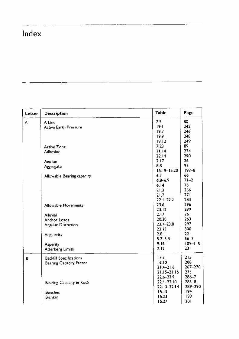
Index
Letter Description Table Page
A A-Line 7.5 80Active Earth Pressure 19.1 242
19.7 24619.9 24819.12 249
Active Zone 7.23 89Adhesion 21.14 274
22.14 290Aeolian 2.17 26Aggregate 8.8 95
15.19-15.20 197-8Allowable Bearing capacity 6.3 66
6.8-6.9 71-26.14 7521.3 26621.7 27122.1-22.2 283
Allowable Movements 23.6 29623.12 299
Alluvial 2.17 26Anchor Loads 20.20 263Angular Distortion 23.7-23.8 297
23.13 300Angularity 2.8 22
5.7-5.8 56-7Asperity 9.16 109-110Atterberg Limits 2.12 23
B Backfill Specifications 17.3 215Bearing Capacity Factor 16.10 208
21.4-21.6 267-27021.15-21.16 27522.6-22.9 286-7
Bearing Capacity in Rock 22.1-22.10 283-822.13-22.14 289-290
Benches 15.13 194Blanket 15.23 199
15.27 201
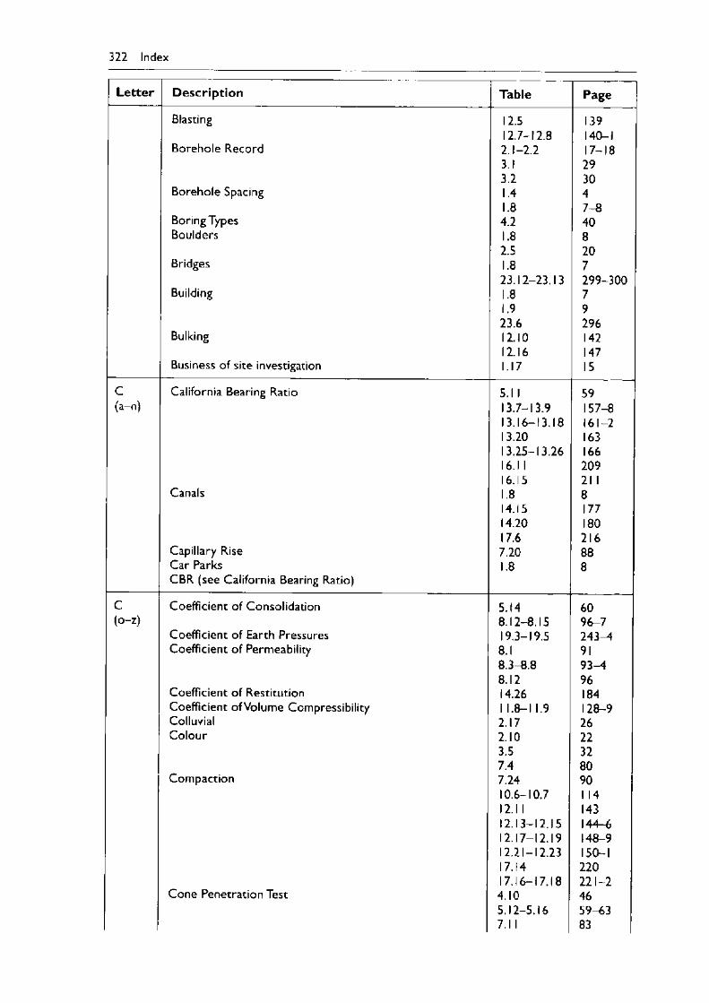
322 Index
Letter D escription Table Page
Blasting 12.5 13912.7-12.8 140-1
Borehole Record 2.1-2.2 17-183.1 293.2 30
Borehole Spacing 1.4 41.8 7-8
Boring Types 4.2 40Boulders 1.8 8
2.5 20Bridges 1.8 7
23.12-23.13 299-300Building 1.8 7
1.9 923.6 296
Bulking 12.10 14212.16 147
Business of site investigation 1.17 15
C California Bearing Ratio 5.1 1 59(a-n) 13.7-13.9 157-8
13.16-13.18 161-213.20 16313.25-13.26 16616.1 1 20916.15 21 1
Canals 1.8 814.15 17714.20 18017.6 216
Capillary Rise 7.20 88Car Parks 1.8 8CBR (see California Bearing Ratio)
C Coefficient of Consolidation 5.14 60(o-z) 8.12-8.15 96-7
Coefficient of Earth Pressures 19.3-19.5 243—4Coefficient of Permeability 8.1 91
8.3-8.8 93-18.12 96
Coefficient of Restitution 14.26 184Coefficient ofVolume Compressibility i 1.8-1 1.9 128-9Colluvial 2.17 26Colour 2.10 22
3.5 327.4 80
Compaction 7.24 9010.6-10.7 1 1412.1 1 14312.13-12.15 144-612.17-12.19 148-912.21-12.23 150-117.14 22017.16-17.18 221-2
Cone Penetration Test 4.10 465.12-5.16 59-637.1 1 83
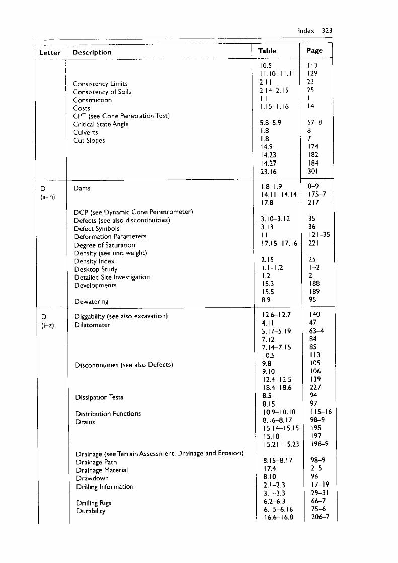
Index 323
L e tte r D escrip tion Tab le Page
Consistency Limits Consistency of Soils Construction CostsC PT (see Cone Penetration Test) Critical State Angle Culverts Cut Slopes
10.5 1 1.10-1 1.11 2.1 12.14-2.15 l.l1.15-1.16
5.8-5.9 1.8 1.8 14.9 14.23 14.27 23.16
1 13 129 23 25 114
57-887174182184301
D Dams 1.8-1.9 8-9(a-h) 14.1 1-14.14 175-7
17.8 217D CP (see Dynamic Cone Penetrometer)Defects (see also discontinuities) 3.10-3.12 35Defect Symbols 3.13 36Deformation Parameters 1 1 121-35Degree of Saturation 17.15-17.16 221Density (see unit weight)Density Index 2.15 25Desktop Study 1.1-1.2 1-2Detailed Site Investigation 1.2 2Developments 15.3 188
15.5 189Dewatering 8.9 95
D Diggability (see also excavation) 12.6-12.7 140(i-z) Dilatometer 4.1 1 47
5.17-5.19 63—47.12 847.14-7.15 8510.5 113
Discontinuities (see also Defects) 9.8 1059.10 10612.4-12.5 13918.4-18.6 227
Dissipation Tests 8.5 948.15 97
Distribution Functions 10.9-10.10 115-16Drains 8.16-8.17 98-9
15.14-15.15 19515.18 19715.21-15.23 198-9
Drainage (see Terrain Assessment, Drainage and Erosion)Drainage Path 8.15-8.17 98-9Drainage Material 17.4 215Drawdown 8.10 96Drilling Information 2.1-2.3 17-19
3.1-3.3 29-31Drilling Rigs 6.2-6.3 66-7Durability 6.15-6.16 75-6
| 16.6-16.8 206-7
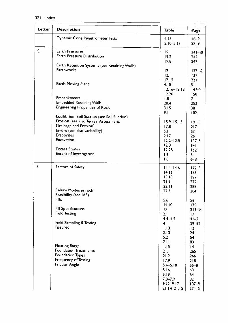
324 Index
L ette r D escrip tion Table Page
Dynamic Cone Penetrometer Tests 4.15 48-95.10-5.1 1 58-9
E Earth Pressures 19 241 —SOEarth Pressure Distribution 19.2 242
19.8 247Earth Retention Systems (see Retaining Walls)Earthworks 12 137-32
12.1 13717.15 221
Earth Moving Plant 4.18 5112.16-12.18 147—c12.20 150
Embankments 1.8 7Embedded Retaining Walls 20.4 253Engineering Properties of Rock 3.15 38
9.1 102Equilibrium Soil Suction (see Soil Suction)Erosion (see also Terrain Assessment, 15.9-15.12 I9 I- :Drainage and Erosion) 17.8 217Errors (see also variability) 5.1 53Evaporites 2.17 26Excavation 12.2-12.5 I3 7 -C
12.8 141Excess Stones 12.25 152Extent of Investigation 1.6 5
1.8 6-8
F Factors of Safety 14.4-14.6 I72-:14.1 1 17515.18 19721.9 27222.1 1 288
Failure Modes in rock 22.3 284Feasibility (see IAS)Fills 5.6 56
14.10 175Fill Specifications 17 213-/4Field Testing 2.1 17
4.4-4.5 41-2Field Sampling & Testing 4 39-52Fissured 1.13 12
2.13 245.2 54 j7.1 1 83
Floating Barge 1.15 14Foundation Treatments 21.1 265Foundation Types 21.2 266Frequency ofTesting 17.9 218Friction Angle 5.4-5.10 55-8
5.16 635.19 647.8-7.9 829.12-9.17 107-921.14-21.15 274-5
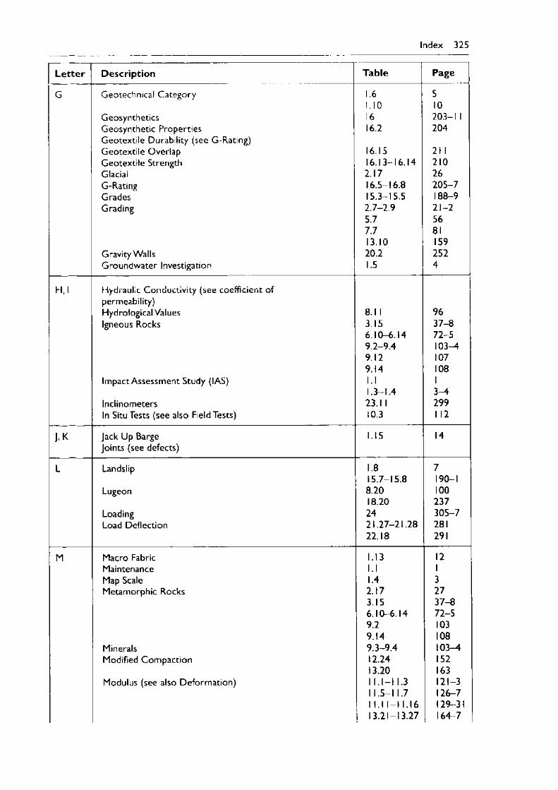
Index 325
L ette r Description Table Page
G Geotechnical Category
GeosyntheticsGeosynthetic PropertiesGeotextile Durability (see G-Rating)Geotextile OverlapGeotextile StrengthGlacialG-RatingGradesGrading
Gravity WallsGroundwater Investigation
1.61.101616.2
16.1516.13-16.142.1716.5-16.8 15.3-15.5 2.7-2.95.77.7 13.10 20.2 1.5
510203-11 204
21 1 210 26205-7188-921-256811592524
H .l Hydraulic Conductivity (see coefficient ofpermeability)Hydrological Values 8.1 1 96Igneous Rocks 3.15 37-8
6.10-6.14 72-59 2 -9 .4 103—49.12 1079.14 108
Impact Assessment Study (IAS) 1.1 11.3-1.4 3-4
Inclinometers 23.1 1 299In Situ Tests (see also Field Tests) 10.3 1 12
J.K Jack Up Barge 1.15 14Joints (see defects)
L Landslip 1.8 715.7-15.8 190-1
Lugeon 8.20 10018.20 237
Loading 24 305-7Load Deflection 21.27-21.28 281
22.18 291
M Macro Fabric 1.13 12Maintenance l.l 1Map Scale 1.4 3Metamorphic Rocks 2.17 27
3.15 37-86.10-6.14 72-59.2 1039.14 108
Minerals 9.3-9.4 103—4Modified Compaction 12.24 152
13.20 163Modulus (see also Deformation) 1 l . l - l 1.3 121-3
1 1.5-1 1.7 126-71 l. l l - l 1.16 129-3113.21-13.27 164-7
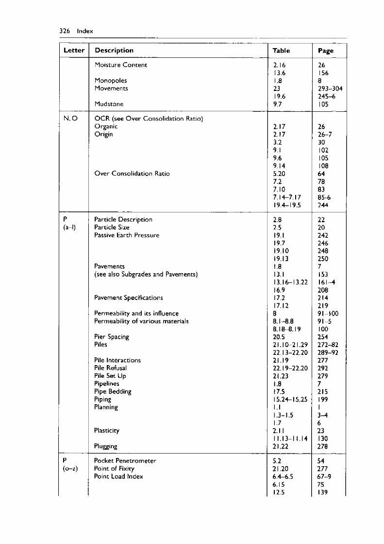
326 Index
L e tte r D escription Table Page
Moisture Content 2.16 2613.6 156
Monopoles 1.8 8Movements 23 293-304
19.6 245-6Mudstone 9.7 105
N, O O C R (see O ver Consolidation Ratio)Organic 2.17 26Origin 2.17 26-7
3.2 309.1 1029.6 1059.14 108
O ver Consolidation Ratio 5.20 647.2 787.10 837.14-7.17 85-619.4-19.5 244
P Particle Description 2.8 22(a-l) Particle Size 2.5 20
Passive Earth Pressure 19.1 24219.7 24619.10 24819.13 250
Pavements 1.8 7(see also Subgrades and Pavements) 13.1 153
13.16-13.22 161-416.9 208
Pavement Specifications 17.2 21417.12 219
Permeability and its influence 8 91-100Permeability of various materials 8.1-8.8 91-5
8.18-8.19 100Pier Spacing 20.5 254Piles 21.10-21.29 272-82
22.13-22.20 289-92Pile Interactions 21.19 277Pile Refusal 22.19-22.20 292Pile Set Up 21.23 279Pipelines 1.8 7Pipe Bedding 17.5 215Piping 15.24-15.25 199Planning l.l 1
1.3-1.5 3-11.7 6
Plasticity 2.1 1 231 1.13-1 1.14 130
Plugging 21.22 278
P Pocket Penetrometer 5.2 54(o-z) Point of Fixity 21.20 277
Point Load Index 6.4-6.5 67-96.15 7512.5 139
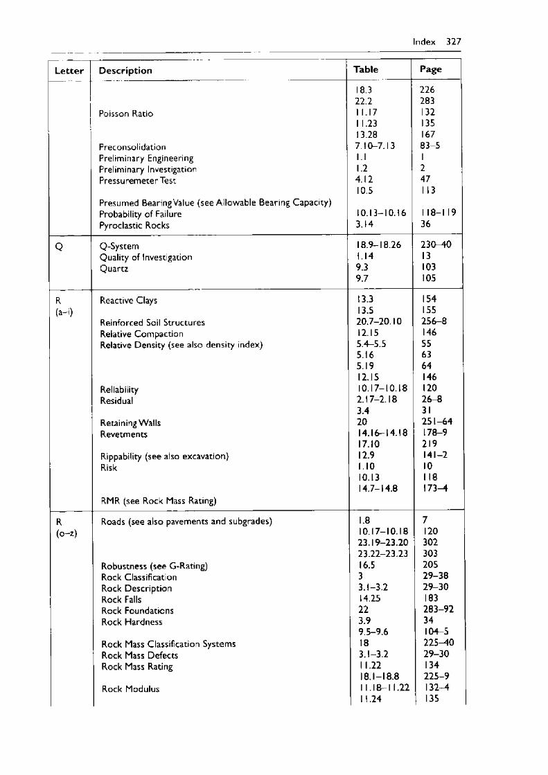
Index 327
Letter Description Table Page
Poisson Ratio
Preconsolidation Preliminary Engineering Preliminary Investigation Pressuremeter Test
Presumed Bearing Value (see Allowable Bearing Capacity) Probability of Failure Pyroclastic Rocks
18.3 22.2 1 1.17 1 1.23 13.28 7.10-7.13 l.l 1.2 4.12 10.5
10.13-10.163.14
22628313213516783-51247113
118-119 36
Q Q-System 18.9-18.26 230-40Quality of Investigation 1.14 13Quartz 9.3 103
9.7 105
R Reactive Clays 13.3 154(a-i) 13.5 155
Reinforced Soil Structures 20.7-20.10 256-8Relative Compaction 12.15 146Relative Density (see also density index) 5.4-5.5 55
5.16 635.19 6412.15 146
Reliability 10.17-10.18 120Residual 2.17-2.18 26-8
3.4 31Retaining Walls 20 251-64Revetments 14.16-14.18 178-9
17.10 219Rippability (see also excavation) 12.9 141-2Risk 1.10 10
10.13 1 1814.7-14.8 173—4
RMR (see Rock Mass Rating)
R Roads (see also pavements and subgrades) 1.8 7(o-z) 10.17-10.18 120
23.19-23.20 30223.22-23.23 303
Robustness (see G-Rating) 16.5 205Rock Classification 3 29-38Rock Description 3.1-3.2 29-30Rock Falls 14.25 183Rock Foundations 22 283-92Rock Hardness 3.9 34
9.5-9.6 104-5Rock Mass Classification Systems 18 225—40Rock Mass Defects 3.1-3.2 29-30Rock Mass Rating 1 1.22 134
18.1-18.8 225-9Rock Modulus 1 1.18-1 1.22 132—4
1 1.24 135
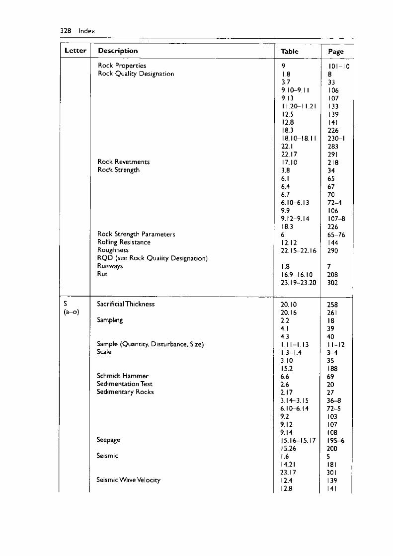
328 Index
L e tte r D escription Table Page
Rock Properties 9 101-10Rock Quality Designation 1.8 8
3.7 339.10-9.1 1 1069.13 1071 1.20-1 1.21 13312.5 13912.8 14118.3 22618.10-18.1 1 230-122.1 28322.17 291
Rock Revetments 17.10 218Rock Strength 3.8 34
6.1 656.4 676.7 706.10-6.13 72-49.9 1069.12-9.14 107-818.3 226
Rock Strength Parameters 6 65-76Rolling Resistance 12.12 144Roughness 22.15-22.16 290R Q D (see Rock Quality Designation)Runways 1.8 7Rut 16.9-16.10 208
23.19-23.20 302
S Sacrificial Thickness 20.10 258(a—o) 20.16 261
Sampling 2.2 184.1 394.3 40
Sample (Quantity, Disturbance, Size) l.l 1-1.13 1 1-12Scale 1.3-1.4 3-4
3.10 3515.2 188
Schmidt Hammer 6.6 69Sedimentation Test 2.6 20Sedimentary Rocks 2.17 27
3.14-3.15 36-86.10-6.14 72-59.2 1039.12 1079.14 108
Seepage 15.16-15.17 195-615.26 200
Seismic 1.6 514.21 18123.17 301
Seismic Wave Velocity 12.4 13912.8 141
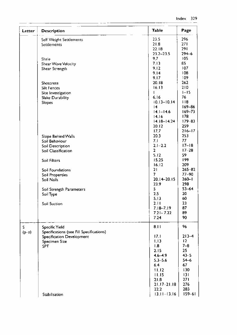
Index 329
Letter Description Table Page
Self Weight Settlements 23.5 296Settlements 21.8 271
22.18 29123.2-23.5 294—6
Shale 9.7 105Shear Wave Velocity 7.13 85Shear Strength 9.12 107
9.14 1089.17 109
Shotcrete 20.18 262Silt Fences 16.13 210Site Investigation 1 1-15Slake Durability 6.16 76Slopes 10.13-10.14 1 18
14 169-8614.1-14.6 169-7314.16 17814.18-14.24 179-8320.12 25917.7 216-17
Slope Behind Walls 20.3 253Soil Behaviour 7.1 77Soil Description 2.1-2.2 17-18Soil Classification 2 17-28
5.12 59Soil Filters 15.25 199
16.12 209Soil Foundations 21 265-82Soil Properties 7 77-90Soil Nails 20.14-20.15 260-1
23.9 298Soil Strength Parameters 5 53-64Soil Type 2.5 20
5.13 60Soil Suction 2.1 1 23
7.18-7.19 877.21- 7.22 897.24 90
S Specific Yield 8.1 1 96(p-z) Specifications (see Fill Specifications)
Specification Development 17.1 213-4Specimen Size 1.13 12SPT 1.8 7-8
2.15 254.6—4.9 43-55.3-5.6 54-66.4 6711.12 13011.15 13121.8 27121.17-21.18 27622.2 283
Stabilisation 13.1 1-13.16 159-61
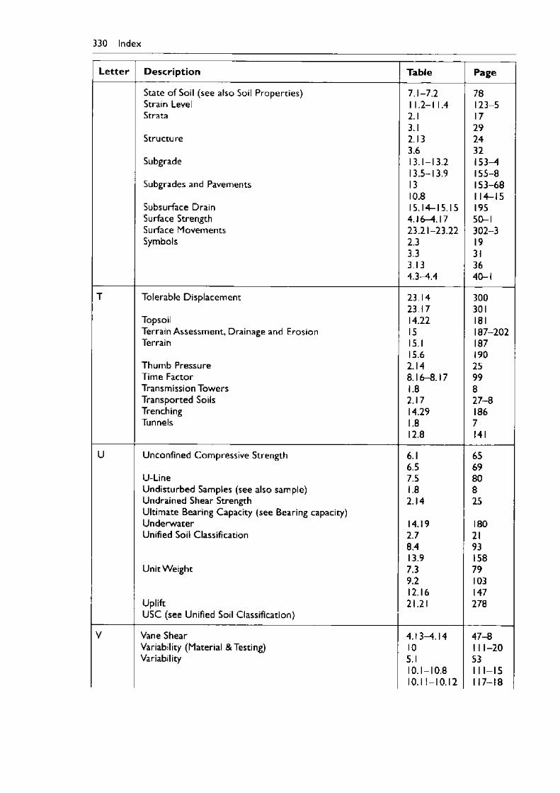
330 Index
Lette r D escription Table Page
State of Soil (see also Soil Properties) 7.1-7.2 78Strain Level 1 1.2-1 1.4 123-5Strata 2.1 17
3.1 29Structure 2.13 24
3.6 32Subgrade 13.1-13.2 153—4
13.5-13.9 155-8Subgrades and Pavements 13 153-68
10.8 114-15Subsurface Drain 15.14-15.15 195Surface Strength 4.16-4.17 50-1Surface Movements 23.21-23.22 302-3Symbols 2.3 19
3.3 313.13 364.3—4.4 40-1
T Tolerable Displacement 23.14 30023.17 301
Topsoil 14.22 181Terrain Assessment, Drainage and Erosion 15 187-202Terrain 15.1 187
15.6 190Thumb Pressure 2.14 25Time Factor 8.16-8.17 99Transmission Towers 1.8 8Transported Soils 2.17 27-8Trenching 14.29 186Tunnels 1.8 7
12.8 141
U Unconfined Compressive Strength 6.1 656.5 69
U-Line 7.5 80Undisturbed Samples (see also sample) 1.8 8Undrained Shear Strength 2.14 25Ultimate Bearing Capacity (see Bearing capacity)Underwater 14.19 180Unified Soil Classification 2.7 21
8.4 9313.9 158
Unit Weight 7.3 799.2 10312.16 147
Uplift 21.21 278U SC (see Unified Soil Classification)
V Vane Shear 4.13-4.14 47-8Variability (Material & Testing) 10 111-20Variability 5.1 53
10.1-10.8 111-1510.1 1-10.12 117-18
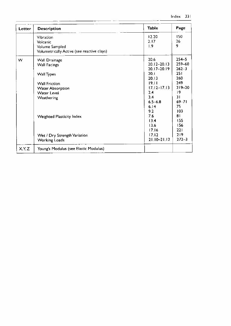
Index 331
Letter D escrip tion Table Page
VibrationVolcanicVolume SampledVolumetrically Active (see reactive clays)
12.202.171.9
150269
W Wall Drainage 20.6 254-5Wall Facings 20.12-20.13 259-60
20.17-20.19 262-3Wall Types 20.1 251
20.13 260Wall Friction 19.1 1 249W ater Absorption 17.12-17.13 219-20W ater Level 2.4 19Weathering 3.4 31
6.5-6.8 69-716.14 759.2 103
Weighted Plasticity Index 7.6 8113.4 15513.6 15617.16 221
W et / D ry Strength Variation 17.12 219Working Loads 21.10-21.12 272-3
X .Y .Z Young’s Modulus (see Elastic Modulus)


Related Documents


