Hammerstein uniform cubic spline adaptive filters: Learning and convergence properties

Contents lists available at ScienceDirect

Signal Processing

Signal Processing 100 (2014) 112–123

0165-16http://d

n CorrE-m

danilo.craffaeleaurelio.

journal homepage: www.elsevier.com/locate/sigpro

Hammerstein uniform cubic spline adaptive filters: Learningand convergence properties

Michele Scarpiniti n, Danilo Comminiello, Raffaele Parisi, Aurelio UnciniDepartment of Information Engineering, Electronics and Telecommunications (DIET),“Sapienza” University of Rome, Via Eudossiana 18,00184 Rome, Italy

a r t i c l e i n f o

Article history:Received 25 July 2013Received in revised form13 January 2014Accepted 20 January 2014Available online 28 January 2014

Keywords:Spline adaptive filterNonlinear adaptive filterLeast mean squareHammerstein system identificationExcess mean square error

84/$ - see front matter & 2014 Elsevier B.V.x.doi.org/10.1016/j.sigpro.2014.01.019

esponding author. Tel.: þ39 06 44585869; faail addresses: [email protected]@uniroma1.it (D. Comminiello),[email protected] (R. Parisi),[email protected] (A. Uncini).

a b s t r a c t

In this paper a novel class of nonlinear Hammerstein adaptive filters, consisting of aflexible memory-less function followed by a linear combiner, is presented. The nonlinearfunction involved in the adaptation process is based on a uniform cubic spline functionthat can be properly modified during learning. The spline control points are adaptivelychanged by using gradient-based techniques. This new kind of adaptive function is thenapplied to the input of a linear adaptive filter and it is used for the identification ofHammerstein-type nonlinear systems. In addition, we derive a simple form of theadaptation algorithm, an upper bound on the choice of the step-size and a lower boundon the excess mean square error in a theoretical manner. Some experimental results arealso presented to demonstrate the effectiveness of the proposed method in theidentification of high-order nonlinear systems.

& 2014 Elsevier B.V. All rights reserved.

1. Introduction

Many efforts have been done by the research commu-nity in the fields of modeling and identification of non-linear systems. While a well established theory is availablein literature for linear filters [1–3], in the nonlinear caseonly approximate models that are acceptable only inproximity of a specific operating point exist and a generaltheoretic framework is not available [1,4].

In order to model nonlinear systems, truncated Volterraseries were introduced [5,6]. Volterra series, one of themost used black-box models, are a generalization of theTaylor series expansion based on convolutive kernel func-tionals. Due to the large number of free parametersrequired, the truncated Volterra Adaptive Filter (VAF)is generally used only in situations of mild nonlinearity

All rights reserved.

x: þ39 06 4873300.(M. Scarpiniti),

[7–10]. Other approaches, simpler than VAF, are based onan a priori fixed nonlinear expansion of the input data intoa higher-dimensional space, where the identification pro-blem can be solved in a linear manner. Examples of thiskind of approaches are represented by Functional LinkAdaptive Filters (FLAFs) [11,12] or Kernel Adaptive Filters(KAFs) [13].

In practice, in nonlinear filtering one of the most usedstructures is the so-called block-oriented representation, inwhich linear time invariant (LTI) models are connectedwith memoryless nonlinear functions [14]. The basicclasses of block-oriented nonlinear systems are repre-sented by the Wiener and Hammerstein models [4] andby those system architectures originated by the connec-tion of these two classes according to different topologies(i.e. parallel, cascade, and feedback) [15]. More specifically,the Wiener model consists of a cascade of a linear LTI filterfollowed by a static nonlinear function and sometimes isknown as linear–nonlinear (LN) model [16–18]. The Ham-merstein model, which consists of a cascade connection ofa static nonlinear function followed by a LTI filter [19,20],is sometimes indicated as nonlinear–linear (NL) model.

M. Scarpiniti et al. / Signal Processing 100 (2014) 112–123 113

In addition, sandwich models, such as the linear–non-linear–linear (LNL) or the nonlinear–linear–nonlinear (NLN)models, were also introduced [1,21]. Of particular interestit has been the estimation of the specialized classes ofHammerstein systems. In fact, Hammerstein architecturescan be successfully used in several applications in all fieldsof engineering, from signal processing [22–24], to biome-dical data analysis [25,26] or other applications, likehydraulics [27] or chemistry processes [28].

Actually, many existing methods for Hammersteinsystem identification are not adaptive [19,29]. On the otherhand, adaptive methods, both parametric and non-para-metric, are usually based on the use of some particular andfixed nonlinearities [22,30–32].

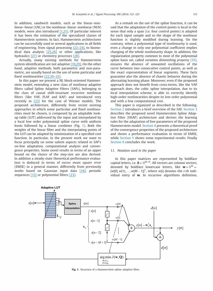
In this paper we present a NL block-oriented Hammer-stein model, extending a new class of nonlinear adaptivefilters called Spline Adaptive Filters (SAFs), belonging tothe class of causal shift-invariant recursive nonlinearfilters (like VAF, FLAF and KAF) and introduced veryrecently in [33] for the case of Wiener models. Theproposed architecture, differently from recent existingapproaches in which some particular and fixed nonlinea-rities must be chosen, is composed by an adaptable look-up table (LUT) addressed by the input and interpolated bya local low order polynomial spline curve with uniformknots followed by a linear combiner (Fig. 1). Both theweights of the linear filter and the interpolating points ofthe LUT can be adapted by minimization of a specified costfunction. In particular, in the present work we want tofocus principally on some salient aspects related to SAF'son-line adaptation, computational analysis and conver-gence properties. Some novel results in terms of an upperbound on the choice of the step-size are also derived.In addition a steady-state theoretical performance evalua-tion is deduced in terms of excess mean square error(EMSE) in a general manner, differently from previouslyworks based on Gaussian input data [34], periodicsequences [12] or polynomial filters [23].

[ ]s n

[ 1]s n

[ 2]s n

[ 1]s n M

ns

1z

1z

argminQ

wQ

w

QL

Adaptive LUT

Spline

interpolation

[ ]x n [ ]s n

_

_

_

_

_ +

∈Ω∈Ω

Fig. 1. Structure of a Hammerst

As a remark on the use of the spline function, it can besaid that the adaptation of the control points is local in thesense that only a span (i.e. four control points) is adaptedfor each input sample and so the shape of the nonlinearfunction is slightly modified during learning. On thecontrary, when a polynomial type of nonlinearity is used,even a change in only one polynomial coefficient implieschanging of the whole nonlinearity shape. In addition, theregularization property common to most of the polynomialspline basis set, called variation diminishing property [35],ensures the absence of unwanted oscillations of thecurve between two consecutive control points, as well asthe exact representation of linear segments. These factsguarantee also the absence of chaotic behavior during thealternating learning phase. Moreover, even if the proposedapproach does not benefit from cross-terms, like the VAFapproach does, the cubic spline interpolation, due to itslocal interpolation scheme, is able to correctly identifyhigh-order nonlinearities despite its low order polynomialand with a low computational cost.

This paper is organized as described in the following.Section 2 introduces a brief overview of the SAF. Section 3describes the proposed novel Hammerstein Spline Adap-tive Filter (HSAF) architecture and derives the learningrules for the adaptation of free parameters of the proposedHammerstein model. Section 4 presents a theoretical proofof the convergence properties of the proposed architectureand shows a performance evaluation in terms of EMSE,while Section 5 shows some experimental results. FinallySection 6 concludes the work.

1.1. Notation used in the paper

In this paper matrices are represented by boldfacecapital letters, i.e. AARM�N . All vectors are column vectors,denoted by boldface lowercase letters, like wARM ¼½w½0�;w½1�;…;w½M�1��T , where w½i� denotes the i-th indi-vidual entry of w. In recursive algorithms definition,

[0]w

[ ] Tn ny n w s

[ ]d n

[ ]y n

[ ]e n

( , )J w Q

[ 1]w M

[1]w

_

_=

ein spline adaptive filter.

1 In this work we consider only real-valued variables.

M. Scarpiniti et al. / Signal Processing 100 (2014) 112–123114

discrete-time subscript index n is added. For example, theweight vector, calculated according to some law, can bewritten as wnþ1 ¼wnþΔwn. In the case of signal regres-sion, vectors are indicated as snARM ¼ ½s½n�; s½n�1�;…; s½n�Mþ1��T , or sn�1ARM ¼ ½s½n�1�; s½n�2�;…;

s½n�M��T . Note that in the absence of temporal indexs� sn by default.

2. Brief review on SAF

For a complete introduction on spline adaptive filteringand spline interpolation, we refer to our recent paper [33].

In summary, with reference to Fig. 1, in order tocompute the linear filter input s½n� ¼ φðx½n�Þ, that is auniform spline interpolation of some adaptive controlpoints contained in a LUT, we have to determine theexplicit dependence between the input signal x½n� ands½n�. This can be easily done by considering that s½n� is afunction of two local parameters un and i which depend onx½n�. In the simple case of uniform spacing of knots and athird-order curve interpolation adopted in this work, thecomputation procedure for the determination of the spanindex i and the local parameters un can be expressed bythe following equations [36]:

un ¼x½n�Δx

� x½n�Δx

� �;

i¼ x½n�Δx

� �þ Q�1

2; ð1Þ

where Δx is the uniform space between knots, ⌊�c is thefloor operator and Q is the total number of control points.The second term in the second equation is an offset valueneeded to force i to be always nonnegative. Note that theindex i is really depending from time n, i.e. in; forsimplicity of notation we adopt the convention in � i.

Referring to the top of Fig. 2 and to [33], the output ofthe nonlinearity can be evaluated as

s½n� ¼ φiðunÞ ¼ uTnCqi;n ð2Þ

where, considering a third-order spline basis, the matrixCAR4�4 is a pre-computed matrix, usually called splinebasis matrix, the vector un is defined as unAR4�1 ¼½u3

n u2n un 1�T , and the vector qi;n contains the control

points at instant n and is defined by qi;nAR4�1 ¼½qi qiþ1 qiþ2 qiþ3�T , where qk is the k-th entry in the LUT.We call the two blocks expressed by (1) and (2) as S1 andS2, respectively (see Fig. 2).

It could be very important to evaluate the derivative of(2) with respect to its input. It is easily evaluated in

φ0iðunÞ ¼ _uT

nCqi;n; ð3Þ

where _unAR4�1 ¼ ½3u2n 2un 1 0�T .

3. Hammerstein spline adaptive filter

There exist several ways to approach the Hammersteinidentification problem [37]. In this paper we use thestandard stochastic gradient method. With reference toFigs. 1 and 2, let us pose e½n� the output error that is

defined as

e½n� ¼ d½n��y½n� ¼ d½n��wTn � sn; ð4Þ

where snARM�1 ¼ ½s½n�; s½n�1�;…; s½n�Mþ1��T and eachsample s½n�k� is evaluated by using (2).

The on-line learning algorithm can be derived byconsidering the cost function1 (CF) Jðwn;qi;nÞ ¼ Efe2½n�g.As usual, this CF is approximated by considering only theinstantaneous error

Jðwn;qi;nÞ ¼ e2½n�: ð5Þ

For the minimization of (5), we proceed by applying thestochastic gradient adaptation. At the time-index n we canwrite

∂Jðwn;qi;nÞ∂wn

¼ �2e n½ � ∂y½n�∂wn

; ð6Þ

where y½n� ¼wTnsn. Hence (6) becomes

∂Jðwn;qi;nÞ∂wn

¼ �2e n½ �sn: ð7Þ

For the derivative computation of (5) with respect to thecontrol points qi;n, we apply the chain rule

∂Jðwn;qi;nÞ∂qi;n

¼ 2e n½ � ∂ðd½n��y½n�Þ∂qi;n

¼ �2e n½ � ∂y½n�∂sn

∂sTn∂qi;n

; ð8Þ

From (2), we have that ∂sTn=∂qi;n ¼ CTUi;n, where Ui;nAR4�M ¼ ½ui;n;ui;n�1;…;ui;n�Mþ1� is a matrix which collectsM past vectors ui;n�k, each one assuming the value ofun�k if it was evaluated in the same span i of the currentsample input x½n� or in an overlapped span, otherwise it isa zero vector. So we can write

∂Jðwn;qi;nÞ∂qi;n

¼ �2e n½ �CTUi;nwn: ð9Þ

Note that, in (9) the update at time-index n is dependingon past samples of the spline local parameter un. The Ui;n

matrix, not so easy to be calculated, is essential to correctlyevaluate the derivative ∂sTn=∂qi;n. This is similar to the back-propagation through time algorithm for neural networks[38]. This behavior is different from the Wiener case [33]where the derivative of the cost function with respect thespline control points is depending on the current inputsample alone.

Finally, indicating explicitly the time index n, the LMSiterative learning algorithm can be written as

wnþ1 ¼wnþμw½n�e½n�sn; ð10Þ

qi;nþ1 ¼ qi;nþμq½n�e½n�CTUi;nwn; ð11Þ

where the parameters μw½n� and μq½n�, represent thelearning rates for the weights and for the control pointsat time instant n respectively and, for simplicity, incorpo-rate the others constant values. In the next section ananalytical derivation of a bound for these learning rates ispresented.

It can be noted that at each iteration all the weights arechanged, whereas only the four control points of the

S1 S2[ ]x n

[ ]s n

u

i

u x

x

iq 1iq 2iq 3iq

iq

i

, nx q [ 1]s n

[ 1]s n M

1z

1z[ ]y n

ns

[0]w

[1]w

[ 1]w M

+ + +

∆

∆

)(φ

_

_

_

_

_

+

Fig. 2. Schematic structure of the proposed Hammerstein SAF. Block S1 computes the local parameters u and i by (1), while S2 computes the spline outputby (2). qi denotes the vector collecting the local control points, while Δx is the uniform space between two consecutive control points. For simplicity ofnotation we use qi;n � qi , un � u and in � i.

M. Scarpiniti et al. / Signal Processing 100 (2014) 112–123 115

involved curve span are updated. This is a consequence ofthe locality of the spline interpolation scheme.

A summary of the proposed LMS algorithm for thenonlinear Hammerstein architecture can be found inAlgorithm 1.

Algorithm 1. Summary of the Hammerstein SAF-LMSalgorithm.

1: for n¼ 0;1;… do2: un ¼ x½n�=Δx�⌊x½n�=Δxc3: i¼ ⌊x½n�=ΔxcþðQ�1Þ=24: s½n� ¼ uT

nCqi;n

5: y½n� ¼wTnsn

6: e½n� ¼ d½n��y½n�7: wnþ1 ¼wnþμw½n�e½n�sn8: Ui;n ¼ ½ui;n;ui;n�1 ;…;ui;n�Mþ1�9: qi;nþ1 ¼ qi;nþμq ½n�e½n�CTUi;nwn

10: end for

The learning expressions (10) and (11) can be simplygeneralized to second order learning rules like quasi-Newton(QN) [39], Recursive Least Squares (RLS) [40], Affine Projec-tion Algorithm (APA) [41] or other variants [2].

3.1. Computational analysis

For the computational cost analysis we refer to ourprevious work [33], where a comprehensive analysis isperformed.

In summary, for each iteration only the i-th span of thecurve is modified by calculating the quantities un, i and the

expressions uTnCqi;n and CTUi;n appearing respectively in

the 4-th and 8-th lines in Algorithm 1. However, most ofthe computations can be done through the re-use of pastcalculations. The cost for the spline output computationand its adaptation is 4KM multiplication, plus 4KA addi-tions, where KM and KA are constants (less than 16),depending of the implementation structure (see for exam-ple [36]). In any case, for high deep memory SAF, wherethe filter length is Mb4, the computational overhead, forthe nonlinear function computation and its adaptation,can be neglected with respect to a simple linear filter.

4. Convergence properties

In order to achieve optimal performance, it is crucialthat the learning rate, used in gradient-based adaptation,is able to adjust in accordance with the dynamics of theinput signal x½n� and the nonlinearity φiðunÞ [42]. For thispurpose, it is useful to adopt an adaptive learning rate thatminimizes the instantaneous output error of the filter [43].

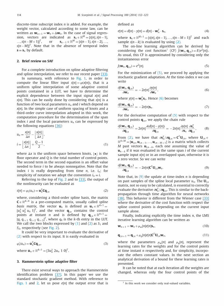
Fig. 3 shows the model to be identified (denoted withsubscript 0), and the adaptive architecture adopted. Theconvergence properties can be achieved by performing aTaylor expansion of the output error e½n�, that is a nonlinearfunction of the filter input x½n�. The method determines theoptimal learning rate in order to assure the convergence.

The cost function (5) depends on two variables. In thissense it is easy to verify that it cannot admit a uniquesolution so that limn-1 Efwng ¼w0 and limn-1 Efqng ¼q0, because the variables w and q are not independent.However, the adaptation can be performed in two separatephases. For example, the filter weights coefficients w can

Fig. 3. Adaptive identification scheme used for statistical performance evaluation.

M. Scarpiniti et al. / Signal Processing 100 (2014) 112–123116

be preemptively adapted in the first phase of learning. Inthis way, the hypothesis that the change in weights can beminimal during the last phase of adaptation can beconsidered true.

4.1. Stability

The convergence property of the (10) can be derivedfrom the Taylor series expansion of the error e½nþ1�around the instant n, stopped at the first order [44,45]

e nþ1½ � ¼ e n½ �þ ∂e½n�∂wT

nΔwnþh:o:t:; ð12Þ

where h.o.t. means high order terms. Now, using (4) and(10), we derive

∂e½n�∂wT

n¼ �sTn; ð13Þ

Δwn ¼ μw½n�e½n�sn: ð14ÞSubstituting (13) and (14) in (12), we can obtain aftersimple manipulations

e½nþ1� ¼ ð1�μw½n�:sn:2Þe½n�: ð15Þ

In order to ensure the convergence of the algorithm, wedesire that 9e½nþ1�9o9e½n�9. This aim is reached if thefollowing relation holds

91�μw½n�:sn:29o1; ð16Þ

that implies the following bound on the choice of thelearning rate μw½n�

0oμw n½ �o 2

:sn:2 : ð17Þ

Note that in (17) all quantities are positive, thus no posi-tivity constrains are needed. Now it is s½n� ¼ φðx½n�;qi;nÞ,hence expanding the function φð�Þ in Taylor series, weobtain

s½n� ¼ φðx½n�;qi;nÞ ¼ φiðunÞ � φið0Þþunφ0ið0Þ: ð18Þ

Now using the expressions (2) and (3), it is possible toderive

φið0Þ ¼ c4qi;n; ð19Þ

φ0ið0Þ ¼ c3qi;n; ð20Þ

where ckAR1�4 is the k-th row of the C matrix.Hence, let us pose unARM�1 ¼ ½un;un�1;…;un�Mþ1�T

the vector that collects the variable un at temporal instantsn;n�1;…;n�Mþ1 and Q i;n the 4�M matrix collectingthe qi;n vectors at temporal instants n;n�1;…;n�Mþ1,it is possible to write (18) in a vectorial form as

sn �Q Ti;nc

T4þun Q T

i;ncT3; ð21Þ

where is the element-wise product. Thus Eq. (17) bec-omes

0oμw n½ �r 2

:Q Ti;ncT4þun Q T

i;ncT3:2 : ð22Þ

Constraint (22) shows that the convergence propertiesdepend on the particular basis of spline function, due tothe terms c3 and c4 and the spacing between knots, sincethe terms un are depending from Δx.

In order to stabilize the expression in (17) due tounsatisfactory statistics for nonlinear and nonstationaryinput signals, an adaptable regularizing term δw½n� can beadded. So the learning rate is chosen as

μw n½ � ¼ 2

:sn:2þδw½n�

: ð23Þ

The regularizing term δw½n� can be adapted by using agradient descent approach [45,46]:

δw½nþ1� ¼ δw½n��ηw∇δw Jðwn;qi;nÞ; ð24Þ

where ηw is the learning rate. For the evaluation of thegradient in (24), we use the chain rule

∇δw J wn;qi;n

� �¼ ∂Jðwn;qi;nÞ∂δw½n�

¼ ∂Jðwn;qi;nÞ∂e½n�

∂e½n�∂y½n� �

∂y½n�∂wT

n

∂wn

∂μw½n�∂μw½n�∂δw½n�

¼ 4e½n�e½n�1�sTnsn�1

ð:sn:2þδw½n�1�Þ2: ð25Þ

Hence, we derive

δw nþ1½ � ¼ δw n½ ��ηwe½n�e½n�1�sTnsn�1

ð:sn:2þδw½n�1�Þ2: ð26Þ

M. Scarpiniti et al. / Signal Processing 100 (2014) 112–123 117

Note that in (26) the terms sn and sn�1 depend on thevalue of the nonlinear adaptive function and its derivativein the origin φið0Þ and φ0

ið0Þ, using (18) or (21).In a similar way, we can derive a bound on μq½n�. From

the Taylor series expansion of the error e½nþ1� around theinstant n, stopped at the first order, we obtain

e nþ1½ � ¼ e n½ �þ ∂e½n�∂qT

i;n

Δqi;nþh:o:t; ð27Þ

and, from (4) and (11), the equations

∂e½n�∂qT

i;n

¼ �CTUi;nwn; ð28Þ

Δqi;n ¼ μq½n�e½n�CTUi;nwn: ð29ÞHence we derive, after simple manipulations

e½nþ1� ¼ ½1�μq½n�:CTUi;nwn:2�e½n�: ð30Þ

In order to ensure the convergence of the algorithm,imposing the uniform convergence of (30) as done in (16),we obtain

91�μq½n�:CTUi;nwn:29o1; ð31Þ

that implies the following bound on the choice of thelearning rate μq½n�

0oμq n½ �o 2

:CTUi;nwn:2 : ð32Þ

Eqs. (17) and (32) impose on the learning rates simpleconstraints. A more restrictive constraint must be satisfiedby μw½n� and μq½n� simultaneously. In order to obtain such acondition, rewrite the output error expansion as

e nþ1½ � ¼ e n½ �þ∂e½n�∂wT

n

����qn ¼ const

Δwnþ∂e½n�∂qT

n

����wn ¼ const

Δqn:

ð33ÞUsing (13), (14), (28) and (29), Eq. (33) can be rewritten as

e½nþ1� ¼ e½n�½1�μw½n�:sn:2�μq½n�:CTUi;nwn:2�: ð34Þ

Imposing once again the condition 9e½nþ1�9o9e½n�9, wefinally obtain the constraint

0oμw½n�:sn:2þμq½n�:CTUi;nwn:2o2: ð35Þ

4.2. Mean square performance

The aim of this paragraph is to study the mean squareperformance of the proposed architecture at steady-state.In particular we are interested in the derivation of theexcess mean square error (EMSE) of the nonlinear adaptivefilter [2]. Even in this case the analysis is performed in aseparate manner, considering first the case of the linearfilter and then the nonlinear spline function. Note that forEMSE evaluation we are interested in steady-state, so thefixed sub-system can be considered adapted. In the follow-ing we denote with ɛ½n� the a priori error of the wholesystem in Fig. 3, with ɛw½n� the a priori error when only thelinear filter is adapted while the spline control points arefixed and similarly with ɛq½n� the a priori error when only

the control points are adapted while the linear filter isfixed. In order to make tractable the mathematical deriva-tion, some assumption must be introduced:

A1. The noise sequence v½n� is i.i.d. with variance sv2

and zero mean.A2. The noise sequence v½n� is independent of xn, sn,

ɛ½n�, ɛw½n� and ɛq½n�.

Let us define the weight error vector as vðwÞn ¼w0�wn.

From (10) we can write

vðwÞnþ1 ¼ vðwÞ

n �μw½n�e½n�sn: ð36Þ

Now let us evaluate the a priori error ɛw½n� ¼ d½n��y½n�when only the linear filter with parameters wn is adapted.We obtain

ɛw½n� ¼wT0rn�wT

nsn � ðw0�wnÞTsn ¼ vðwÞTn sn; ð37Þ

where rn ¼ ½r½n�; r½n�1�;…; r½n�Mþ1��T and r½n� ¼ φðx½n�;q0Þ is the output of the reference nonlinearity. In (37) we usethe approximation rn � sn, and hence qn � q0, that can beconsidered a reasonable assumption at steady-state.

Now evaluating the energies of both sides of (36), weobtain

:vðwÞnþ1:

2 ¼ :vðwÞn :2�2μw½n�e½n�ɛw½n�þμ2w½n�e2½n�:sn:

2: ð38Þ

Taking the expectation of both sides of (38) and notingthat, at steady-state for n-1, is Ef:vðwÞ

nþ1:2g ¼ Ef:vðwÞ

n :2g,it can be obtained

2Efe½n�ɛw½n�g ¼ μw½n�Efe2½n�:sn:2g: ð39Þ

Remembering that e½n� ¼ ɛw½n�þv½n�, where v½n� is anadditive noise on reference signal (see Fig. 3) that isuncorrelated with the a priori error for assumption A2[47], we can easily derive

Efe½n�ɛw½n�g ¼ Efðɛw½n�þv½n�Þɛw½n�g ¼ Efɛ2w½n�g: ð40ÞSince :sn:

2 is the steady-state L2 norm, and justified fromthe fact that at steady-state the error is very small, wehave

Efe2½n�:sn:2g ¼ Efðɛw½n�þv½n�Þ2:sn:2g¼ :sn:

2½Efɛ2w½n�gþs2v �; ð41Þ

where s2v is the variance of the noise v½n� (assumption A1).Inserting (40) and (41) in (39), it is possible to derive

2Efɛ2w½n�g ¼ μw½n�½Efɛ2w½n�gþs2v �:sn:2: ð42Þ

Denoting with ζw ¼ limn-1 Efɛ2w½n�g the EMSE on thelinear filter, from (42) we finally obtain

ζw ¼ μw½n�s2v:sn:2

2�μw½n�:sn:2: ð43Þ

For the consistency of ζw in (43), it is necessary that theEMSE is a positive value. For this purpose, we impose thepositivity of the denominator of (43). This easily leads toEq. (17).

If the learning rate μw½n� is very small, the second termin the denominator of (43) can be neglected, so the

2 Some Matlab source codes, implementing the experimental results,are available at the following web page: http://ispac.ing.uniroma1.it/HSAF.html.

M. Scarpiniti et al. / Signal Processing 100 (2014) 112–123118

expression of EMSE reduces to

ζw ¼ μw½n�2

s2v:sn:2: ð44Þ

It is interesting to note that the derivatives of Eqs. (43) and(44) with respect to the learning rate μw½n� are alwayspositive, hence the EMSE has not a minimum value and anoptimum value for μw½n� is not existing.

With a similar reasoning, starting from the definition ofcontrol-point error vector vðqÞn ¼ q0�qn and (11), we obtain

vðqÞnþ1 ¼ vðqÞn �μq½n�e½n�CTUi;nwn: ð45ÞEvaluating now the a priori error ɛq½n�, we obtain

ɛq½n� ¼wT0rn�wT

nsn �wTn � ðrn�snÞ

¼wTn � UT

i;nC � ðq0�qnÞ ¼wTnU

Ti;nCv

ðqÞn ; ð46Þ

in which we use the approximation w0 �wn, that can beconsidered a reasonable assumption at steady-state. Eval-uating now the energies of both sides of (45) we obtain

:vðqÞnþ1:2 ¼ :vðqÞn :2�2μq½n�e½n�ɛq½n�

þμ2q ½n�e2½n�:CTUi;nwn:2: ð47Þ

Taking the expectation and remembering that, for n-1, isEf:vðqÞnþ1:

2g ¼ Ef:vðqÞn :2g, it can be obtained

2Efe½n�ɛq½n�g ¼ μq½n�Efe2½n�:CTUi;nwn:2g: ð48Þ

For assumption A2, it is possible to derive

Efe½n�ɛq½n�g ¼ Efðɛq½n�þv½n�Þɛq½n�g ¼ Efɛ2q ½n�g: ð49Þ

Since :CTUi;nwn:2 is the steady-state L2 norm, and justified

from the fact that at steady-state the error is very small,we have

Efe2½n�:CTUi;nwn:2g ¼ Efðɛq½n�þv½n�Þ2:CTUi;nwn:

2g¼ :CTUi;nwn:

2½Efɛ2q ½n�gþs2v �; ð50Þ

where s2v is the variance of the noise v½n� (assumption A1).Hence, we can derive

2Efɛ2q ½n�g ¼ μq½n�½Efɛ2q ½n�gþs2v �:CTUi;nwn:2: ð51Þ

Denoting with ζq ¼ limn-1 Efɛ2q ½n�g the EMSE concerningthe spline control points q, from (42) we finally obtain

ζq ¼μq½n�s2v:CTUi;nwn:

2

2�μq½n�:CTUi;nwn:2 : ð52Þ

For the consistency of ζq in (52), we impose the positivityof the denominator of (52). This easily leads to (32). If thelearning rate μq½n� is very small, (52) reduces to

ζq ¼μq½n�2

s2v:CTUi;nwn:

2: ð53Þ

A similar conclusion on the nonexistence of an optimumvalue for μq½n� can be done.

Now it can be considered that the a priori error ɛ½n� ofthe whole system is due to the error ɛw½n� due to the filtertaps and the error ɛq½n� due to the control points. In fact,using (37) and (46), we obtain

ɛ½n� ¼ d½n��y½n� ¼wT0rn�wT

nsn¼ ðwT

0rn�wT0snÞþðwT

0sn�wTnsnÞ

¼wT0U

Ti;nCðq0�qnÞþðw0�wnÞTsn

�wTnU

Ti;nCv

ðqÞn þvðwÞT

n sn ¼ ɛw½n�þɛq½n�: ð54Þ

Hence

ζ¼ limn-1

Efɛ2½n�g ¼ limn-1

Efðɛw½n�þɛq½n�Þ2g

¼ limn-1

Efɛ2w½n�gþ limn-1

Efɛ2q ½n�gþ2 limn-1

Efɛw½n�ɛq½n�g¼ ζwþζqþ2ζwqZζwþζq; ð55Þ

where ζwq ¼ limn-1 Efɛw½n�ɛq½n�g denotes the cross-EMSE.When errors ɛw½n� and ɛq½n� could be considered statisti-cally independent and zero mean then ζwq ¼ 0, and theEMSE is the lower possible. Eq. (55) justifies the following

Property 1. The EMSE ζ of a Hammerstein spline adaptivefilter verifies the condition

ζZζwþζq: ð56Þ

From experimental tests we have seen that the simu-lated EMSE is very close to the summation on the rightside of (56) (see Experiment 2), so the errors ɛw½n� andɛq½n� are close to be uncorrelated.

5. Experimental results

In order to validate the proposed nonlinear adaptivefiltering solution, several experiments were performed.Experimental tests address high-order nonlinear systemidentification problem. Uniform cubic spline nonlinearitieshave been used, as they represent a good compromisebetween flexibility and approximation behavior. Compar-isons with two different approaches, in which the non-linearity is implemented by a polynomial function, werealso performed. The first of these approaches is theHammerstein architecture proposed by Stenger and Keller-man in [48], where the linear filter coefficients and thepolynomial coefficients are alternatively adapted by usingan LMS algorithm. The second one is the particularapproach proposed by Jeraj and Mathews in [30] in whicha partial orthogonalization of the inputs signal is performedand the free parameters are adapted all together. Since thelatter approach considers an IIR linear filter, in order toperform a substantial comparison between all architec-tures, only the MA part of the linear filter is considered.

During the validation phase of our work, we performedmany experimental tests, but for paper length optimization,and in order to focus on the simplicity of the proposedapproach, we have decided to present only six experiments.2

Due to the local scheme of spline interpolation, the possi-bility of chaotic behavior, as underlined in Section 1, couldbe excluded: in fact we never observed such a chaoticbehavior in experimental sessions, and always a good resultis obtained if the learning rates are adequately chosen.

As explained in Section 4, although the cost functionmay not admit a unique minimum value and thus the

Table 2Mean values and variance of spline control points in experiment 1averaged over 100 trials, for CR-spline and B-spline respectively.

i q0 CR-spline B-spline

Mean Variance �10�5 Mean Variance �10�5

7 �1.00 �0.996 11.961 �0.995 14.7928 �0.80 �0.796 8.413 �0.797 3.2989 �0.91 �0.906 10.280 �0.906 10.597

10 �0.40 �0.398 1.683 �0.398 0.93711 �0.20 �0.199 0.476 �0.199 0.60412 0.05 0.049 9.059�10�8 0.049 1.451�10�7

13 0.00 �0.000 6.177�10�9 �0.000 3.315�10�7

14 �0.40 �0.398 2.294 �0.372 1.75515 0.58 0.577 3.834 0.539 4.79316 1.00 0.995 12.571 0.952 7.590

−10

0Hammerstein SAF convergence test

q))

MSE a=0.1MSE a=0.95NoiseLevel

M. Scarpiniti et al. / Signal Processing 100 (2014) 112–123 119

convergence toward the optimum cannot be guaranteed,no particular attention should be posed on the choice ofthe initial conditions for the filter weights and splinecontrol points. Without any specific a priori knowledge, areasonable choice of initial conditions that have alwaysguaranteed excellent results is w�1 ¼ αδ for filter weightswith 0oαr1 and δARM�1 ¼ ½1;0;…;0�T , while splinecontrol points q�1 are initialized as a straight line with aunitary slope, i.e. we begin to adapt a linear filter. We haveto emphasize that such a choice, with a positive slope ofthe nonlinearity, avoids the convergence toward �w0 and�q0, preventing a sign ambiguity.

5.1. Experiment 1

A first experiment is performed in order to showthe convergence behavior of the SAF illustrated inSection 4. The experiment consists in the identificationof an unknown Hammerstein system composed by alinear component w0 ¼ ½0:6; �0:4;0:25; �0:15;0:1; �0:05;0:001�T and a nonlinear memoryless target function imple-mented by a 23-points length LUT q0 and interpolated by auniform third degree spline with an interval samplingΔx¼ 0:2 defined as

q0 ¼ f�2:2; �2:0; �1:8;…; �1:0; �0:8; �0:91; �0:40;

�0:20;0:05;0:0; �0:40;0:58;1:0;1:0;1:2;1:4;…;2:2g:The input signal x½n� consists in 30,000 samples of thesignal generated by the following relationship:

x½n� ¼ ax½n�1�þffiffiffiffiffiffiffiffiffiffiffiffiffi1�a2

pξ½n�; ð57Þ

where ξ½n� is a zero mean white Gaussian noise withunitary variance and 0rao1 is a parameter that deter-mines the level of correlation between adjacent samples.Experiments were conducted with a set to 0.1 and 0.95.In addition it is considered as an additive white noise v½n�such that the signal to noise ratio is SNR¼60 dB, whereSNR¼ 10 log10½Efd

2½n�g=Efv2½n�g� (see Fig. 3 for symbolsdefinition). The learning rates are set to μw ¼ μq ¼ 0:1.The filter weights are initialized using α¼0.1.

Results, averaged over 100 trials, are summarized inTable 1, that shows mean values and variances of eachfilter tap, while Table 2 shows mean values and variancesof the most important spline control points. Differentchoices for the C matrix are possible: the most suitable

Table 1Mean values and variance of filter taps in experiment 1 averaged over 100trials, for CR-spline and B-spline respectively.

i w0 CR-spline B-spline

Mean Variance �10�5 Mean Variance �10�5

1 0.60 0.602 4.560 0.602 4.2182 �0.40 �0.401 2.155 �0.402 1.4863 0.25 0.251 0.883 0.251 0.5204 �0.15 �0.150 0.274 �0.151 0.1665 0.10 0.101 0.081 0.101 0.1086 �0.05 �0.050 0.027 �0.051 0.0377 0.001 0.001 1.643�10�8 0.001 7.306�10�8

for this kind of applications are the so-called B-spline andCatmull–Rom spline (or simply CR-spline), introduced in[33] and reported below

CB ¼16

�1 3 �3 13 �6 3 0�3 0 3 01 4 1 0

26664

37775; CCR ¼

12

�1 3 �3 12 �5 4 �1�1 0 1 00 2 0 0

26664

37775:

Both B-spline and CR-spline basis are used in the experi-ment, obtaining similar results.

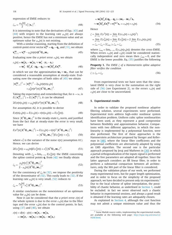
In addition Fig. 4 shows a comparison of the MSEfor the proposed experimental test with the two differentchoices of the parameter a. It is simple to note that,at steady state, the performance of the HSAF algorithmreaches the value of the noise power. Fig. 5 shows acomparison of the profile of the nonlinearity used in themodel (the red dashed line) and the profile of the adaptednonlinearity obtained by spline interpolation in HSAF(the solid black line) when CR-spline is used and a¼0.95.Note that the adapted nonlinearity is well overlapping themodel one, as it is also evident from Table 2.

0 0.5 1 1.5 2 2.5 3

x 104

−70

−60

−50

−40

−30

−20

Samples

MSE

[dB

] 1

0log

(J(w

,

a=0.1

a=0.95

Fig. 4. Comparison of MSE for experiment 1 using model (57) with a¼0.1and 0.95 respectively.

0 0.02 0.04 0.06 0.08 0.1 0.12 0.14 0.16−85

−80

−75

−70

−65

−60

−55

μ

EMSE

[dB

]

Simulated vs. theoretical EMSE

Theoretical EMSESimulated EMSE

Fig. 6. Comparison of theoretical EMSE vs. simulated EMSE.

0 0.5 1 1.5 2 2.5 3 3.5 4 4.5 5

x 104

−30

−25

−20

−15

−10

−5

0

5

10Polynomial filter vs HSAF

Samples

MSE

[dB

] 1

0log

(J(w

,Q))

Fig. 7. Comparison MSE for the different Hammerstein systems inexperiment 3.

−1.5 −1 −0.5 0 0.5 1 1.5

−1.5

−1

−0.5

0

0.5

1

1.5

Profile of spline nonlinearity after learning

Nonlinearity input x[n]

Non

linea

rity

outp

ut s

[n]

TargetSpline

Fig. 5. Comparison of the model and adapted nonlinearity for experi-ment 1 using model (57) with CR-spline basis and a¼0.95. (For interpre-tation of the references to color in this figure caption, the reader isreferred to the web version of this article.)

M. Scarpiniti et al. / Signal Processing 100 (2014) 112–123120

5.2. Experiment 2

In this experiment we prove the validity of (56) inProperty 1. The test consists in the identification of thesame system of the previous experimental test. The inputsignal is (57) with a¼0.1. For simplicity we use μw½n� ¼μq½n� ¼ μ, chosen as the following 12 values:

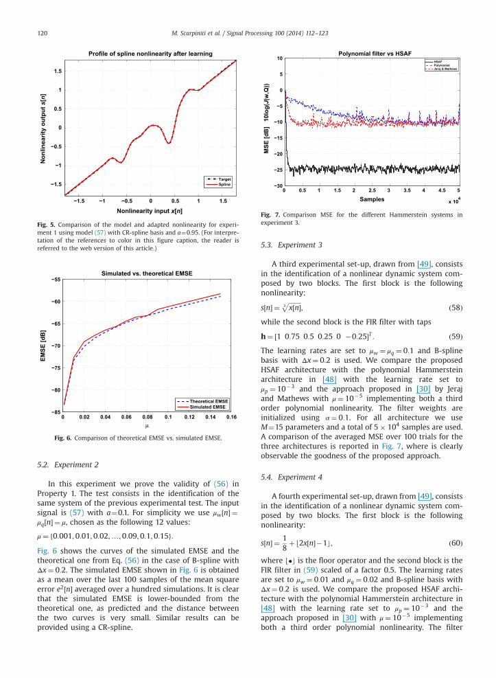
μ¼ f0:001;0:01;0:02;…;0:09;0:1;0:15g:Fig. 6 shows the curves of the simulated EMSE and thetheoretical one from Eq. (56) in the case of B-spline withΔx¼ 0:2. The simulated EMSE shown in Fig. 6 is obtainedas a mean over the last 100 samples of the mean squareerror e2½n� averaged over a hundred simulations. It is clearthat the simulated EMSE is lower-bounded from thetheoretical one, as predicted and the distance betweenthe two curves is very small. Similar results can beprovided using a CR-spline.

5.3. Experiment 3

A third experimental set-up, drawn from [49], consistsin the identification of a nonlinear dynamic system com-posed by two blocks. The first block is the followingnonlinearity:

s½n� ¼ffiffiffiffiffiffiffiffix½n�3

p; ð58Þ

while the second block is the FIR filter with taps

h¼ ½1 0:75 0:5 0:25 0 �0:25�T : ð59ÞThe learning rates are set to μw ¼ μq ¼ 0:1 and B-splinebasis with Δx¼ 0:2 is used. We compare the proposedHSAF architecture with the polynomial Hammersteinarchitecture in [48] with the learning rate set toμp ¼ 10�3 and the approach proposed in [30] by Jerajand Mathews with μ¼ 10�5 implementing both a thirdorder polynomial nonlinearity. The filter weights areinitialized using α¼ 0:1. For all architecture we useM¼15 parameters and a total of 5� 104 samples are used.A comparison of the averaged MSE over 100 trials for thethree architectures is reported in Fig. 7, where is clearlyobservable the goodness of the proposed approach.

5.4. Experiment 4

A fourth experimental set-up, drawn from [49], consistsin the identification of a nonlinear dynamic system com-posed by two blocks. The first block is the followingnonlinearity:

s n½ � ¼ 18þ⌊2x n½ ��1c; ð60Þ

where ⌊�c is the floor operator and the second block is theFIR filter in (59) scaled of a factor 0.5. The learning ratesare set to μw ¼ 0:01 and μq ¼ 0:02 and B-spline basis withΔx¼ 0:2 is used. We compare the proposed HSAF archi-tecture with the polynomial Hammerstein architecture in[48] with the learning rate set to μp ¼ 10�3 and theapproach proposed in [30] with μ¼ 10�5 implementingboth a third order polynomial nonlinearity. The filter

0 0.5 1 1.5 2 2.5 3 3.5 4 4.5 5

x 104

−25

−20

−15

−10

−5

0

5

10Polynomial filter vs HSAF

Samples

MSE

[dB

] 1

0log

(J(w

,Q))

HSAFPolynomialJeraj & Mathews

Fig. 8. MSE of the proposed approach compared different approaches inexperiment 4.

0 0.5 1 1.5 2 2.5 3 3.5 4 4.5 5

x 104

−25

−20

−15

−10

−5

0

5

10Polynomial filter vs HSAF

Samples

MSE

[dB

] 1

0log

(J(w

,Q))

HSAFPolynomialJeraj & Mathews

Fig. 9. Comparison MSE for the different Hammerstein SAF inexperiment 5.

Table 3Comparison MSE for the three different approaches in experiment 6averaged over 100 trials.

Order MSE [dB]

HSAF Polynomial Jeraj and Mathews

3 �49.685 �49.872 �49.9995 �49.192 �49.223 �49.2587 �49.618 �46.563 �46.650

10 �49.791 �40.791 �40.72312 �49.426 �37.418 �37.40615 �49.348 �28.069 �28.037

M. Scarpiniti et al. / Signal Processing 100 (2014) 112–123 121

weights are initialized using α¼ 0:1. For all architecture weuse M¼15 parameters and a total of 5�104 samples areused. A comparison of the averaged MSE over 100 trials forthe two architectures is reported in Fig. 8.

5.5. Experiment 5

A fifth experimental set-up is drawn from [20] andconsists in the identification of the following nonlinearity:

s½n� ¼ x½n��0:3x2½n�þ0:2x3½n� ð61Þfollowed by the 8-th order IIR filter

H zð Þ ¼ 1�1:8000z�1þ1:6200z�2�1:4500z�3þ0:6561z�4

1�0:2314z�1þ0:4318z�2�0:3404z�3þ0:5184z�4

ð62ÞThe learning rates are set to μw ¼ 0:01 and μq ¼ 0:02 andB-spline basis with Δx¼ 0:2 is used. We compare theproposed HSAF architecture with the polynomial Hammer-stein architecture in [48] with the learning rate set toμp ¼ 0:01 and the approach proposed in [30] with μ¼ 10�4

implementing both a third order polynomial nonlinearity.The filter weights are initialized using α¼ 0:1. For allarchitecture we use M¼15 parameters and a total of5�104 samples are used. A comparison of the averagedMSE over 100 trials is reported in Fig. 9, where it can beseen that all three approaches perform in the samemanner. This particular behavior is due to the simplenonlinearity chosen as a third order polynomial, sincethe number of free parameter is the same in all methodsand it is very small.

5.6. Experiment 6

In order to verify that the robustness of the proposedapproach with respect to the increasing of the nonlinearorder, a last experiment is performed. The experimentconsists of a comparison of the HSAF structure, withrespect to the pure polynomial method [48] and theone proposed in [30], in the case of identification of

a polynomial nonlinearity of various order P in theform φðxÞ ¼∑P

k ¼ 1bkxk and a FIR filter with taps w0 ¼

½1; �0:4; 0:25; �0:15; 0:1; �0:05; 0:001�T (the readercan also do other random choice). The input signal is awhite Gaussian noise with zero mean and unitary var-iance; a total of 5�104 samples are used. In addition it isconsidered an additive white noise v½n� such as the SNR is50 dB. Six different polynomials (from 3-rd to 15-th order)are used. In the adaptive algorithms we used a number oflinear coefficients M¼15, and the order of the polynomialnonlinearity is set exactly equal to the one of the model,while a B-spline basis is used. The learning rates are set toμw ¼ 0:01 and μq ¼ 0:02 for HSAF, μw ¼ μp ¼ 0:01 for thepolynomial architecture and μ¼ 10�4 for the Jeraj andMathews algorithm. The filter weights are initialized usingα¼ 0:1 and 100 trials of the algorithms are performed.Comparisons of steady-state MSE, evaluated as a mean ofthe last 100 mean square errors, are shown in Table 3.

This table demonstrates that the proposed approachcan take some advantages in the case of high-ordernonlinearities, since the performances in terms of MSEare quite stable with respect to an increase in the non-linear order, while the performances of the otherapproaches decrease consequently. This result can beexplained by considering the spline's self-regularizationcapabilities related to (1) the local adaptation and (2) the

M. Scarpiniti et al. / Signal Processing 100 (2014) 112–123122

principle of minimal disturbance since a new input datadoes not modify the whole nonlinear shape but only awell-defined portion [50,51]. On the contrary in using apolynomial type of nonlinearity, the adaptation concernsall coefficients that have imply changing of the wholenonlinearity shape.

6. Conclusion

This paper introduces a novel nonlinear Hammersteinadaptive filtering model, where the nonlinearity is imple-mented using spline functions. Splines are flexible non-linear functions, whose shape can be modified during thesimple learning process using gradient-based techniques.A uniform knots spacing is used.

The adaptation of the proposed nonlinear spline adap-tive filter is based on the LMS algorithm. In addition aconstraint on the choice of the learning rate, in order toassure the algorithm convergence, and a lower bound onthe architectural EMSE are also theoretically derived.

Several experimental tests have demonstrated theeffectiveness of the proposed approach. In particular HSAFcan reach good performance with low computational costalso in the case of high-order nonlinearities, against otherexisting approaches.

Acknowledgments

The authors would like to thank all anonymousreviewers for their precious and helpful comments andsuggestions.

References

[1] L. Ljung, System Identification—Theory for the User, 2nd edition,Prentice Hall, Upper Saddle River, N.J., 1999.

[2] A.H. Sayed, Fundamentals of Adaptive Filtering, John Wiley & Sons,Hoboken, New Jersey, 2003.

[3] A. Uncini, Fundamentals of Adaptive Signal Processing, Springer-Verlag, Berlin, 2014.

[4] N. Wiener, Nonlinear Problems in Random Theory, John Wiley &Sons, MIT Press, Cambridge, MA, USA, 1958.

[5] V. Volterra, Sopra le Funzioni che Dipendono da Altre Funzioni,Rendiconti della Reale Accademia Nazionale dei Lincei 3 (1887)97–105. 141–146, 153–158.

[6] V. Volterra, Theory of Functionals and of Integral, and Integral-Differential Equations, Blackie & Son Limited, London and Glasgow,1930.

[7] M. Schetzen, Nonlinear system modeling based on the Wienertheory, Proc. IEEE 69 (12) (1981) 1557–1573.

[8] M. Schetzen, The Volterra and Wiener Theories of NonlinearSystems, John Wiley & Sons, New York, 1980.

[9] V.J. Mathews, G.L. Sicuranza, Polynomial Signal Processing, JohnWiley & Sons, Hoboken, New Jersey, 2000.

[10] J.-M. Le Caillec, Spectral inversion of second order Volterra modelsbased on the blind identification of Wiener models, Signal Process.91 (11) (2011) 2541–2555.

[11] D. Comminiello, M. Scarpiniti, L.A. Azpicueta-Ruiz, J. Arenas-Garcìa,A. Uncini, Functional link adaptive filters for nonlinear acoustic echocancellation, IEEE Trans. Audio Speech Lang. Process. 21 (7) (2013)1502–1512.

[12] A. Carini, G.L. Sicuranza, V.J. Mathews, Efficient adaptive identifica-tion of linear-in-the-parameters nonlinear filters using periodicinput sequences, Signal Process. 93 (5) (2013) 1210–1220.

[13] W. Liu, J.C. Principe, S. Haykin, Kernel Adaptive Filtering: A Com-prehensive Introduction, Wiley, Hoboken, New Jersey, 2010.

[14] F. Giri, E.-W. Bai (Eds.), Block-Oriented Nonlinear System Identifica-tion, Springer-Verlag, Berlin, 2010.

[15] R. Haber, H. Unbehauen, Structure identification of nonlineardynamic systems – a survey on input/output approaches, Automa-tica 26 (4) (1990) 651–677.

[16] E.W. Bai, Frequency domain identification of Wiener models, Auto-matica 39 (2003) 1521–1530.

[17] M. Korenberg, I. Hunter, Two methods for identifying Wienercascades having noninvertible static nonlinearities, Ann. Biomed.Eng. 27 (6) (1999) 793–804.

[18] D. Westwick, M. Verhaegen, Identifying MIMO Wiener systemsusing subspace model identification methods, Signal Process. 52(2) (1996) 235–258.

[19] E.W. Bai, Frequency domain identification of Hammerstein models,IEEE Trans. Autom. Control 48 (2003) 530–542.

[20] I.J. Umoh, T. Ogunfunmi, An affine projection-based algorithm foridentification of nonlinear Hammerstein systems, Signal Process. 90(6) (2010) 2020–2030.

[21] L. Ljung, Identification of nonlinear systems, in: 9th InternationalConference on Control, Automation, Robotics and Vision (ICARCV2006), Singapore, 2006, pp. 1–9.

[22] E.W. Bai, A blind approach to Hammerstein model identification,IEEE Trans. Signal Process. 50 (2002) 1610–1619.

[23] J. Jeraj, V.J. Mathews, Stochastic mean-square performance analysisof an adaptive Hammerstein filter, IEEE Trans. Signal Process. 54 (6)(2006) 2168–2177.

[24] M. Scarpiniti, D. Comminiello, R. Parisi, A. Uncini, Comparison ofHammerstein and Wiener systems for nonlinear acoustic echocancelers in reverberant environments, in: Proceedings of 17thInternational Conference on Digital Signal Processing (DSP2011),Corfu, Greece, 2011, pp. 1–6.

[25] K.J. Hunt, M. Munih, N.N. Donaldson, F.M.D. Barr, Investigation of theHammerstein hypothesis in the modeling of electrically stimulatedmuscle, IEEE Trans. Biomed. Eng. 45 (8) (1998) 99–1009.

[26] S.W. Su, L. Wang, B.G. Celler, A.V. Savkin, Y. Guo, Identification andcontrol of heart rate regulation during treadmill exercise, IEEE Trans.Biomed. Eng. 54 (7) (2007) 1238–1246.

[27] B. Kwak, A.E. Yagle, J.A. Levitt, Nonlinear system identification ofhydraulic actuator friction dynamics using a Hammerstein model,in: Proceedings of the IEEE ASSP'98, vol. 4, Seattle, WA, 1998,pp. 1933–1936.

[28] J.-C. Jeng, L. M.-W., H.-P. Huang, Identification of block-orientednonlinear processes using designed relay feedback tests, Ind. Eng.Chem. Res. 44 (7) (2005) 2145–2155.

[29] Y. Liu, E.W. Bai, Iterative identification of Hammerstein systems,Automatica 43 (2007) 346–354.

[30] J. Jeraj, V.J. Mathews, A stable adaptive Hammerstein filter employ-ing partial orthogonalization of the input signals, IEEE Trans. SignalProcess. 54 (4) (2006) 1412–1420.

[31] Z.Q. Lang, A nonparametric polynomial identification algorithm forthe Hammerstein system, IEEE Trans. Autom. Control 42 (10) (1997)1435–1441.

[32] Q. Shen, F. Ding, Iterative estimation methods for Hammersteincontrolled autoregressive moving average systems based on thekey-term separation principle, Nonlinear Dyn. 75 (2014) 1–8, http://dx.doi.org/10.1007/s11071-013-1097-z.

[33] M. Scarpiniti, D. Comminiello, R. Parisi, A. Uncini, Nonlinear splineadaptive filtering, Signal Process. 93 (4) (2013) 772–783.

[34] N.J. Bershad, P. Celka, J.-M. Vesin, Stochastic analysis of gradientadaptive identification of nonlinear systems with memory forGaussian data and noisy input and output measurements, IEEETrans. Signal Process. 47 (3) (1999) 675–689.

[35] C. de Boor, A Practical Guide to Splines, Revised Edition, Springer-Verlag, Berlin, 2001.

[36] S. Guarnieri, F. Piazza, A. Uncini, Multilayer feedforward networkswith adaptive spline activation function, IEEE Trans. Neural Netw. 10(3) (1999) 672–683.

[37] F. Ding, X.P. Liu, G. Liu, Identification methods for Hammersteinnonlinear systems, Digit. Signal Process. 21 (2) (2011) 215–238.

[38] P. Campolucci, A. Uncini, F. Piazza, B.D. Rao, On-line learningalgorithms for locally recurrent neural networks, IEEE Trans. NeuralNetw. 10 (2) (1999) 253–271.

[39] D.F. Marshall, W.K. Jenkins, A fast quasi-Newton adaptive filteringalgorithm, IEEE Trans. Signal Process. 40 (7) (1992) 1652–1662.

[40] J.M. Cioffi, T. Kailath, Fast recursive least-squares transversal filtersfor adaptive filtering, IEEE Trans. Acoust. Speech Signal Process. 32(2) (1984) 304–337.

M. Scarpiniti et al. / Signal Processing 100 (2014) 112–123 123

[41] K. Ozeki, T. Umeda, An adaptive filtering algorithm using anorthogonal projection to an affine subspace and its properties,Electron. Commun. Jpn. 67-A (5) (1984) 19–27.

[42] S. Kalluri, G.R. Arce, General class of nonlinear normalized adaptivefiltering algorithms, IEEE Trans. Signal Process. 47 (8) (1999)2262–2272.

[43] V.J. Mathews, X. Zhenhua, A stochastic gradient adaptive filter withgradient adaptive step size, IEEE Trans. Signal Process. 41 (6) (1993)2075–2087.

[44] D.P. Mandic, J.A. Chambers, Recurrent Neural Networks for Predic-tion, John Wiley & Sons, Baffins Lane, England, 2001.

[45] D.P. Mandic, A.I. Hanna, M. Razaz, A normalized gradient descentalgorithm for nonlinear adaptive filters using a gradient adaptivestep size, IEEE Signal Process. Lett. 8 (11) (2001) 295–297.

[46] D.P. Mandic, A generalized normalized gradient descent algorithm,IEEE Signal Process. Lett. 11 (2) (2004) 115–118.

[47] N.R. Yousef, A.H. Sayed, A unified approach to the steady-state andtracking analyses of adaptive filters, IEEE Trans. Signal Process. 49(2) (2001) 314–324.

[48] A. Stenger, W. Kellerman, Adaptation of a memoryless preprocessorfor nonlinear acoustic echo cancelling, Signal Process. 80 (9) (2000)1747–1760.

[49] Z. Hasiewicz, M. Pawlak, P. Sliwinski, Nonparametric identificationof nonlinearities in block-oriented systems by orthogonal waveletswith compact support, IEEE Trans. Circuits Syst.—I: Regul. Pap. 52 (2)(2005) 427–442.

[50] L. Vecci, F. Piazza, A. Uncini, Learning and approximation capabilitiesof adaptive spline activation function neural networks, Neural Netw.11 (2) (1998) 259–270.

[51] M. Solazzi, A. Uncini, Regularizing neural networks using flexiblemultivariate activation function, Neural Netw. 17 (2004) 247–260.