Hamilton’s Principle in Continuum Mechanics A. Bedford University of Texas at Austin

Welcome message from author
This document is posted to help you gain knowledge. Please leave a comment to let me know what you think about it! Share it to your friends and learn new things together.
Transcript

Hamilton’s Principlein Continuum Mechanics
A. BedfordUniversity of Texas at Austin

This document contains the complete text of the monograph published in 1985by Pitman Publishing, Ltd. Copyright by A. Bedford.
1
Contents
Preface 4
1 Mechanics of Systems of Particles 81.1 The First Problem of the Calculus of Variations . . . . . . . . . . 81.2 Conservative Systems . . . . . . . . . . . . . . . . . . . . . . . . 12
1.2.1 Hamilton’s principle . . . . . . . . . . . . . . . . . . . . . 121.2.2 Constraints . . . . . . . . . . . . . . . . . . . . . . . . . . 15
1.3 Nonconservative Systems . . . . . . . . . . . . . . . . . . . . . . 17
2 Foundations of Continuum Mechanics 202.1 Mathematical Preliminaries . . . . . . . . . . . . . . . . . . . . . 20
2.1.1 Inner Product Spaces . . . . . . . . . . . . . . . . . . . . 202.1.2 Linear Transformations . . . . . . . . . . . . . . . . . . . 222.1.3 Functions, Continuity, and Differentiability . . . . . . . . 242.1.4 Fields and the Divergence Theorem . . . . . . . . . . . . 25
2.2 Motion and Deformation . . . . . . . . . . . . . . . . . . . . . . . 272.3 The Comparison Motion . . . . . . . . . . . . . . . . . . . . . . . 322.4 The Fundamental Lemmas . . . . . . . . . . . . . . . . . . . . . . 36
3 Mechanics of Continuous Media 393.1 The Classical Theories . . . . . . . . . . . . . . . . . . . . . . . . 40
3.1.1 Ideal Fluids . . . . . . . . . . . . . . . . . . . . . . . . . . 403.1.2 Elastic Solids . . . . . . . . . . . . . . . . . . . . . . . . . 463.1.3 Inelastic Materials . . . . . . . . . . . . . . . . . . . . . . 50
3.2 Theories with Microstructure . . . . . . . . . . . . . . . . . . . . 543.2.1 Granular Solids . . . . . . . . . . . . . . . . . . . . . . . . 543.2.2 Elastic Solids with Microstructure . . . . . . . . . . . . . 59
2

4 Mechanics of Mixtures 654.1 Motions and Comparison Motions of a Mixture . . . . . . . . . . 66
4.1.1 Motions . . . . . . . . . . . . . . . . . . . . . . . . . . . . 664.1.2 Comparison Fields . . . . . . . . . . . . . . . . . . . . . . 68
4.2 Mixtures of Ideal Fluids . . . . . . . . . . . . . . . . . . . . . . . 714.2.1 Compressible Fluids . . . . . . . . . . . . . . . . . . . . . 714.2.2 Incompressible Fluids . . . . . . . . . . . . . . . . . . . . 734.2.3 Fluids with Microinertia . . . . . . . . . . . . . . . . . . . 75
4.3 Mixture of an Ideal Fluid and an Elastic Solid . . . . . . . . . . . 834.4 A Theory of Mixtures with Microstructure . . . . . . . . . . . . . 86
5 Discontinuous Fields 915.1 Singular Surfaces . . . . . . . . . . . . . . . . . . . . . . . . . . . 915.2 An Ideal Fluid Containing a Singular Surface . . . . . . . . . . . 98
Acknowledgments 101
Bibliography 102
3

Preface
The good of Hamilton is not in what he has done but in the work (notnearly half done) which he makes other people do. But to understandhim you should look him up, and go through all kinds of sciences,then you go back to him, and he tells you a wrinkle.
James Clerk Maxwell
In 1808, when he was two years old, William Rowan Hamilton was sent to livewith an aunt and uncle, Elizabeth and James Hamilton, in Trim, County Meath.James Hamilton was a classics scholar and graduate of Trinity College Dublin,and was headmaster of a diocesan school for boys. He soon recognized thathis nephew showed extraordinary promise, and gave him intensive training inlanguages and the classics.
While he prepared for entrance to Trinity College, Hamilton became inter-ested in mathematics, particularly analytic geometry. At the age of seventeenhe was reading Theorie des Fonctions Analytiques and Mecanique Analytiqueby Lagrange in addition to the books prescribed for the undergraduate sciencecourse at Trinity.
At Trinity College, Hamilton pursued a dual course in science and theclassics—although he found it increasingly difficult to maintain his interest inthe latter—and also began independent research on geometric optics as a naturalextension of his interest in analytic geometry. His work led to a paper, “Theoryof Systems of Rays” [37], which he presented to the Royal Irish Academy inApril, 1827. Primarily on the basis of his original researches in optics, he waselected to the position of Andrews Professor of Astronomy at Trinity College inJune, 1827.
Hamilton’s theory of ray optics was a variational theory. It was based on theprinciple, due to Fermat, that a light ray traveling between two points will followthe path that requires the least time. In the course of his work on optics, healso began to consider the possibility of developing an analogous theory for the
4

dynamics of systems of particles. This resulted, in 1834–1835, in two papers,“On a General Method in Dynamics” [38] and “Second Essay on a GeneralMethod in Dynamics” [39]. In the second paper he presented the result that isknown today as Hamilton’s principle.
Hamilton’s general and elegant work on dynamics was widely quoted but notextensively applied during the remainder of the nineteenth century. However,when quantum mechanics was developed, it was realized that Hamilton’s workwas the most natural setting for its formulation. In fact, in retrospect Hamilton’sformal analogy between optics and classical mechanics was seen as a precursorof wave mechanics.
A somewhat similar historical development has occurred in the field of con-tinuum mechanics. Although formulations of Hamilton’s principle for continuabegan to appear as early as 1839, with the exception of applications to struc-tural analysis variational methods in continuum mechanics were regarded asacademic, because the same results could be obtained using more direct meth-ods. Some modern treatises on continuum mechanics do not mention variationalmethods. In recent years, however, interest in variational methods has increasedmarkedly. They have been used to obtain approximate solutions, as in the finiteelement method, and to study the stability of solutions to problems in fluidand solid mechanics. Variational formulations have also been used to developgeneralizations of the classical theories of fluid and solid mechanics.
The objective of this monograph is to give a comprehensive account of theuse of Hamilton’s principle to derive the equations that govern the mechanicalbehavior of continuous media. The classical theories of fluid and solid mechanicsare discussed as well as two generalizations of those theories for which Hamilton’sprinciple is particularly suited—materials with microstructure and mixtures.
These topics are brought together for the first time to acquaint readers whoare new to this subject with an interesting and powerful alternative approachto the formulation of continuum theories. Persons interested in fluid and solidmechanics will gain a broadened perspective on those subjects as well as learnthe fundamental background required to read the large literature on variationalmethods in continuum mechanics. For readers who are familiar with thesemethods, a number of recent results are presented on applications of Hamilton’sprinciple to generalized continua and materials containing singular surfaces.These results are presented in a setting that could encourage generalizationsand extensions.
Hamilton’s principle was originally expressed in terms of the classical me-chanics of systems of particles. The concepts and the terminology involved in
5

applying Hamilton’s principle to continuum mechanics are quite similar, andsome familiarity with the applications to systems of particles is very helpfulin understanding the extension to the case of a continuum. The applicationof Hamilton’s principle to systems of particles is therefore briefly discussed inChapter 1. This subject provides a simple context in which to introduce thevariational ideas underlying Hamilton’s principle as well as the method of La-grange multipliers and the concept of virtual work.
Chapter 2 provides a brief survey of the mathematics and elements of con-tinuum mechanics that are required in the subsequent chapters. Most of thischapter can be skipped by persons familiar with modern continuum mechanics;however, even those who are acquainted with variational methods in continuummechanics should briefly examine Section 2.3 before proceeding to the followingchapters.
Applications of Hamilton’s principle to a continuous medium are described inChapter 3. Ideal fluids and elastic solids are treated in Sections 3.1.1 and 3.1.2.The general case of a continuum that does not exhibit microstructural effectsis presented in Section 3.1.3. Section 3.2 presents applications of Hamilton’sprinciple to two particular theories of materials with microstructure. Theseapplications illustrate the use of Hamilton’s principle to generalize the ordinarytheories of fluid and solid mechanics. Persons who are new to this subject maychoose to omit this section and the following chapter in a first reading.
As another example of the use of Hamilton’s principle to develop generalizedcontinuum theories, applications to mixtures are described in Chapter 4. Thefact that the sum of the volume fractions of the constituents of a mixture mustequal one at each point can be introduced into Hamilton’s principle using themethod of Lagrange multipliers. As a result of “wrinkles” such as this, Hamil-ton’s principle provides a simple and elegant way to derive continuum theoriesof mixtures. A mixture of ideal fluids is discussed in Section 4.2. The case of aliquid containing a distribution of gas bubbles is treated as an example, includ-ing the microkinetic energy associated with bubble oscillations. In Section 4.3,a mixture of an ideal fluid and an elastic material is considered, and it is shownthat the equations obtained through Hamilton’s principle are equivalent to theBiot equations. A theory of mixtures of materials with microstructure in whichthe constituents need not be ideal or elastic is presented in Section 4.4.
In Chapter 5 a discussion is given of the application of Hamilton’s princi-ple to a continuous medium containing a surface across which the fields thatcharacterize the medium, or their derivatives, suffer jump discontinuities. Thefundamental results required to include a singular surface in a statement of
6

Hamilton’s principle are presented in Section 5.1. An elastic fluid is treated asan example in Section 5.2, and it is shown that Hamilton’s principle yields thejump conditions of momentum and energy across the surface.
The results presented in this monograph are expressed in a modern frame-work. Persons wishing to gain an impression of Hamilton’s research in its origi-nal form should consult his collected works [40], [41]. The definitive references onHamilton’s life are Graves [32] and Hankins [42]. In Chapters 1-3, the sourcesthat have been used are cited, but no attempt is made to give complete ororiginal references except for results that are relatively recent. In Chapters 2and 3, particular reference is made to works by M. E. Gurtin. The responsibil-ity for errors or misinterpretations of course rests with the author. Chapters 4and 5 are based in large part on work done by the author in collaboration withD. S. Drumheller and G. Batra during the last ten years. One motivation forwriting this monograph was to present these results in their classical context,together with a complete discussion of the foundations.
Hamilton’s research anticipated modern trends in mechanics in two respects.He approached problems primarily from the perspective of a mathematician,and he consistently sought the greatest possible generality in his results. It is ameasure of his success that, one hundred and fifty years after the publication ofhis two great works on mechanics, his results continue to find new and fruitfulapplications.
7

Chapter 1
Mechanics of Systems ofParticles
1.1 The First Problem of the Calculus of Vari-ations
Before Hamilton’s principle is introduced, some preliminary comments on thecalculus of variations are necessary. Hamilton’s principle is closely related towhat is called the first problem of the calculus of variations, which can be in-troduced by a simple example.
Let x be a real variable, and let the closed interval x1 ≤ x ≤ x2 be denotedby [x1, x2]. A function y(x) is said to be CN on [x1, x2] if the N th derivative ofy(x) exists and is continuous on [x1, x2]. The value of a derivative at an endpointis defined to be the limit of the derivative as the endpoint is approached fromwithin the interval.
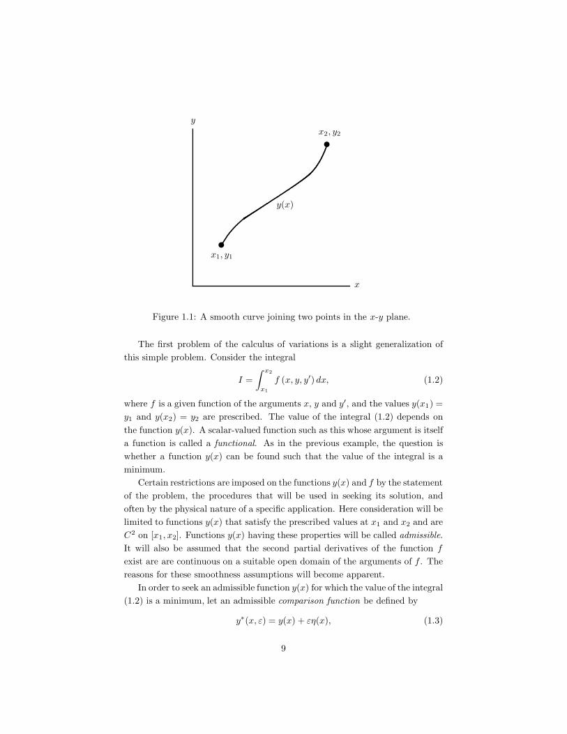
Let x1, y1 and x2, y2 be two fixed points in the x-y plane, with x1 < x2, andlet y(x) be a C1 function on [x1, x2] such that y(x1) = y1 and y(x2) = y2. Thusy(x) describes a smooth curve that joins the two points, as shown in Figure 1.1.
The length of the curve joining the two points is
L =∫ x2
x1
√1 + (y′)2 dx, (1.1)
where y′ = dy/dx. Consider the following question: Can a smooth curve joiningthe two points be found such that its length is a minimum in comparison withother such curves? That is, among functions y(x) that are C1 on [x1, x2] andsatisfy the conditions y(x1) = y1 and y(x2) = y2, can one be found for whichthe value of the integral (1.1) is a minimum?
8
u
u
x
y
y(x)
x1, y1
x2, y2
Figure 1.1: A smooth curve joining two points in the x-y plane.
The first problem of the calculus of variations is a slight generalization ofthis simple problem. Consider the integral
I =∫ x2
x1
f (x, y, y′) dx, (1.2)
where f is a given function of the arguments x, y and y′, and the values y(x1) =y1 and y(x2) = y2 are prescribed. The value of the integral (1.2) depends onthe function y(x). A scalar-valued function such as this whose argument is itselfa function is called a functional. As in the previous example, the question iswhether a function y(x) can be found such that the value of the integral is aminimum.
Certain restrictions are imposed on the functions y(x) and f by the statementof the problem, the procedures that will be used in seeking its solution, andoften by the physical nature of a specific application. Here consideration will belimited to functions y(x) that satisfy the prescribed values at x1 and x2 and areC2 on [x1, x2]. Functions y(x) having these properties will be called admissible.It will also be assumed that the second partial derivatives of the function f
exist are are continuous on a suitable open domain of the arguments of f . Thereasons for these smoothness assumptions will become apparent.
In order to seek an admissible function y(x) for which the value of the integral(1.2) is a minimum, let an admissible comparison function be defined by
y∗(x, ε) = y(x) + εη(x), (1.3)
9

where ε is a parameter and η(x) is an arbitrary C2 function on [x1, x2] subjectto the requirements that η(x1) = 0 and η(x2) = 0 (see Figure 1.2). If thecomparison function (1.3) is substituted into the integral (1.2) in place of thefunction y(x), the integral becomes
I∗(ε) =∫ x2
x1
f(x, y∗, y∗′
)dx, (1.4)
where it is indicated that the value of the integral is a function of the parame-ter ε.
u
u
x
y
y(x)
y∗(x, ε)
x1, y1
x2, y2
Figure 1.2: The function y(x) and the comparison function y∗(x, ε).
Now let it be assumed that the value of the integral (1.4) is a minimumwhen the comparison function y∗(x, ε) = y(x). That is, the function I∗(ε) is aminimum when the parameter ε = 0, which implies the necessary condition
[dI∗(ε)dε
]
ε=0
= 0. (1.5)
The derivative of (1.4) with respect to ε is
dI∗(ε)dε
=∫ x2
x1
(∂f∗
∂y∗∂y∗
∂ε+∂f∗
∂y∗′∂y∗′
∂ε
)dx
=∫ x2
x1
(∂f∗
∂y∗η +
∂f∗
∂y∗′η′)dx (1.6)
where f∗ = f(x, y∗, y∗′
)and η′ = dη/dx. Therefore the condition (1.5) states
10
that ∫ x2
x1
(∂f
∂yη +
∂f
∂y′η′)dx = 0. (1.7)
The second term in this expression can be integrated by parts to obtain∫ x2
x1
∂f
∂y′η′ dx =
[∂f
∂y′η
]x2
x1
−∫ x2
x1
d
dx
(∂f
∂y′
)η dx. (1.8)
Using this result and recalling that η(x) vanishes at x1 and x2, (1.7) can bewritten ∫ x2
x1
[∂f
∂y− d
dx
(∂f
∂y′
)]η dx = 0. (1.9)
Because the function η(x) is arbitrary subject to the conditions that it be C2
on [x1, x2] and that it vanish at x1 and x2, the expression that multiplies η(x)in the integrand of (1.9) must vanish on [x1, x2]. If this were not the case, afunction η(x) could be chosen so that (1.9) would be violated.
The formal statement of this result is called the fundamental lemma of thecalculus of variations (see e.g. Bolza [12], p. 20):
Suppose that a function ψ(x) is C0 on [x1, x2]. If the equation∫ x2
x1
ψ(x)η(x) dx = 0 (1.10)
holds for every C∞ function η(x) on [x1, x2] that satisfies the condi-tions η(x1) = 0 and η(x2) = 0, then ψ(x) must vanish on [x1, x2].1
Observe that in order to apply this lemma to (1.9), the functions y(x) and fmust be smooth enough so that the expression multiplying η(x) is continuouson [x1, x2]. This is the reason for the differentiability requirements that wereimposed on these functions. Note that
d
dx
(∂f
∂y′
)=
∂2f
∂x∂y′+
∂2f
∂y∂y′y′ +
∂2f
∂y′∂y′y′′, (1.11)
where y′′ = d2y/dx2. Therefore the second derivative of y(x) and the secondpartial derivatives of f must exist and be continuous on [x1, x2].
On the basis of the fundamental lemma, (1.9) implies that
∂f
∂y− d
dx
(∂f
∂y′
)= 0 on [x1, x2] . (1.12)
1A proof of a more general form of this lemma is presented in Section 2.4.
11

This is called the Euler-Lagrange equation. It provides a differential equationwith which to determine the function y(x). In the case of the simple example(1.1), (1.12) yields the equation
y′ = constant, (1.13)
which does describe the curve joining the two points that is of minimum length.The condition (1.5) is obviously only a necessary condition, not a sufficient
condition, for the value of the integral (1.4) to be a minimum when ε = 0.This condition is also satisfied if the value of the integral is a maximum or hasan inflection point of zero slope at ε = 0. Thus the condition (1.5) and thedetermined solution y(x) are necessary conditions given that the value of theintegral is stationary in comparison with neighboring admissible functions.
The open domain on which the second partial derivatives of the function f
must be assumed to exist and be continuous can be defined in retrospect. Itmust encompass the values of the arguments of f associated with the solutiony(x) and with comparison functions (1.3) in a neighborhood of the solution.2
Recommended references on the calculus of variations include Akhiezer [1],Bliss [11], Bolza [12], Courant and Hilbert [15], Finlayson [28], Gelfand andFomin [29], Pars [61], Washizu [73], and Weinstock [74].
1.2 Conservative Systems
1.2.1 Hamilton’s principle
Consider a system of particles whose position, or configuration, can be describedby a set of independent generalized coordinates qk, k = 1, 2, . . . ,K. Let t1 and t2be fixed times, with t1 < t2, and suppose that the configurations of the systemat times t1 and t2 are prescribed. An admissible motion of the system willbe defined to be a set of functions qk(t), k = 1, 2, . . .,K, which satisfy theprescribed values at t1 and t2 and are C2 on [t1, t2].
Let it be assumed that the kinetic energy of the system, T , can be expressedas a function of the generalized coordinates and their time derivatives, T =T (qk, qk). This expression indicates that T may be a function of qk and qk foreach value of k from 1 to K. It will also be assumed that the system is subjectonly to conservative forces and that the potential energy of the system, U , canbe expressed as a function of the generalized coordinates, U = U (qk). Each of
2Henceforth, when a function is said to be continuous with no additional provisos, it willbe understood to be continuous on a suitable open domain of its arguments.
12

the second partial derivatives of T and each of the first partial derivatives of Uwill be assumed to exist and to be continuous.3
What will be called the first form of Hamilton’s principle for a conservativesystem of particles states:
Among admissible motions, the actual motion of a conservative sys-tem is such that the value of the integral
I =∫ t2
t1
(T − U ) dt (1.14)
is stationary in comparison with neighboring admissible motions.
Suppose that the functions qk(t) describe the actual motion of the system.In analogy with (1.3), an admissible comparison motion of the system will bedefined by
qk∗(t, ε) = qk(t) + εηk(t), (1.15)
k = 1, 2, . . .,K, where the ηk(t) are arbitrary C2 functions on [t1, t2] subject tothe requirements that ηk(t1) = 0 and ηk(t2) = 0. Upon substituting (1.15) into(1.14) in place of the functions qk(t), one obtains the integral
I∗(ε) =∫ t2
t1
(T ∗ − U∗) dt, (1.16)
where T ∗ = T (q∗k, q∗k) and U∗ = U (q∗k). Hamilton’s principle states that the
value of this integral is stationary when q∗k(t, ε) = qk(t), which implies that[dI∗(ε)dε
]
ε=0
= 0. (1.17)
The derivative of (1.16) with respect to ε is
dI∗(ε)dε
=∫ t2
t1
(∂T ∗
∂q∗k
∂q∗k∂ε
+∂T ∗
∂q∗k
∂q∗k∂ε
− ∂U∗
∂q∗k
∂q∗k∂ε
)dt
=∫ t2
t1
(∂T ∗
∂q∗kηk +
∂T ∗
∂q∗kηk − ∂U∗
∂q∗kηk
)dt. (1.18)
In this equation, use is made of the summation convention: Whenever an indexappears twice in a single expression, the expression is assumed to be summed
3In the simplest example, the “system” is a single particle. If there are no geometricconstraints on its motion, the generalized coordinates are the three position coordinates ofthe particle relative to a suitable reference frame. The kinetic energy is T = 1
2v · v, where m
is the mass of the particle and v is its velocity vector. The potential energy U is defined suchthat dU = −F · v dt, where F is the force vector acting on the particle. If such a function Uexists, F is said to be conservative.
13

over the range of the index. For example,
∂T ∗
∂q∗k
∂q∗k∂ε
=∂T ∗
∂q∗1
∂q∗1∂ε
+∂T ∗
∂q∗2
∂q∗2∂ε
+ · · ·+ ∂T ∗
∂q∗K
∂q∗K∂ε
. (1.19)
This useful convention will be used throughout this work.From (1.18), the condition (1.17) is
∫ t2
t1
(∂T
∂qkηk +
∂T
∂qkηk − ∂U
∂qkηk
)dt = 0. (1.20)
When the second term is integrated by parts, this equation can be written∫ t2
t1
[∂L
∂qk− d
dt
(∂L
∂qk
)]ηk dt = 0, (1.21)
where L = T − U is the Lagrangian of the system. Because the functions ηk(t)are arbitrary subject to the requirements stated above, they can be assumed tobe nonzero on [t1, t2] for k = 1 only. Equation (1.21) is then of the form (1.10),and the fundamental lemma applies. Repeating this process for each value of kresults in the differential equations
∂L
∂qk− d
dt
(∂L
∂qk
)= 0 on [t1, t2] (1.22)
for each value of k from 1 to K. These are Lagrange’s equations of motion forthe system of particles (see e.g. Goldstein, et al. [30], Chapter 2).
Hamilton’s principle is a postulate regarding the motion of the system. Itembodies the physics of the problem. The mathematical task is to deduce theequations of motion, which are obtained as necessary conditions implied bythe postulate. The number of equations of motion is equal to the number ofindependent generalized coordinates.
As an illustration, consider the motion of a single particle in the x-y plane.Suppose that the particle is subject only to its own weight and let the y axis bedirected upward. The kinetic energy is
T = 12m(x2 + y2
), (1.23)
where m is the mass of the particle, and the potential energy is
U = mgy, (1.24)
where g is the acceleration due to gravity (assumed constant). Equation (1.22)yields the equations of motion
x = 0,y = −g. (1.25)
14

Expressions that depend on the parameter ε have been denoted by an as-terisk. In applications of variational methods, derivatives of such expressionswith respect to ε, evaluated at ε = 0, appear frequently. This can be seen, forexample, in obtaining (1.20) from (1.16) and (1.17). It is therefore convenientto introduce the notation4
δ(·) ≡[∂
∂ε(·)∗]
ε=0
. (1.26)
The symbol δ(·) is called the variation of the expression (·). Observe from (1.15)that
δqk = ηk. (1.27)
Also, From (1.16), the necessary condition (1.17) can be written
∫ t2
t1
δ(T − U ) dt = 0. (1.28)
Stating that this equation holds for admissible comparison functions (1.15) isclearly equivalent to the first form of Hamilton’s principle for a conservativesystem of particles. Therefore, what will be called the second form of Hamilton’sprinciple for such a system states:
Among admissible motions, the actual motion of a conservative sys-tem is such that (1.28) holds.
This is the form in which the principle was stated in Hamilton’s original work[39].
1.2.2 Constraints
Thus far it has been assumed that the generalized coordinates qk are indepen-dent. Suppose instead that they are required to satisfy prescribed equations
αp (qk) = 0, (1.29)
where p = 1, 2, . . . , P , P < K. The first partial derivatives of the functions αp
with respect to each of the qk will be assumed to exist and be continuous.4This notation, which is very common in the literatureon variationalmethods, has acquired
a bad reputation in some circles due to a history of vague definitions and a tendency to useit in performing complicated operations that are bewildering to the uninitiated. After initialattempts to write this monograph without using it, the author decided that it is too usefulto discard. Throughout this work, this notation should be interpreted only as a symbolrepresenting the operation (1.26).
15
Hamilton’s principle can be stated so that it embodies the constraints (1.29)by using the method of Lagrange multipliers (see e.g. Pars [61], Chapter VIII).Let πp(t), p = 1, 2, ..., P , denote a set of functions of time, the Lagrange multi-pliers, that are assumed to be C0 on [t1, t2], and define
C = πpαp. (1.30)
Then the first form of Hamilton’s principle states:
Among admissible motions, the actual motion of a conservative sys-tem subject to the constraints (1.29) is such that the value of theintegral
I =∫ t2
t1
(T − U + C)dt (1.31)
is stationary in comparison with neighboring admissible motions.
In determining the equations of motion, the generalized coordinates qk can betreated as if they are independent ; the constraints (1.29) are accounted for byintroducing them into (1.31) together with the Lagrange multipliers.
Substituting the comparison motions (1.15) into (1.31) in place of the func-tions qk(t) yields the integral
I∗(ε) =∫ t2
t1
(T ∗ − U∗ + C∗) dt, (1.32)
where C∗ = πp(t)αp(q∗k). In this case the condition (1.17) is
∫ t2
t1
[∂L
∂qk− d
dt
(∂L
∂qk
)+ πp
∂αp
∂qk
]ηk dt = 0, (1.33)
and the same argument used to obtain (1.22) results in the differential equationsof motion
∂L
∂qk− d
dt
(∂L
∂qk
)+ πp
∂αp
∂qk= 0 on [t1, t2] (1.34)
for each value of k from 1 to K. Equations (1.29) and (1.34) provide K + P
equations with which to determine the generalized coordinates qk(t) and theLagrange multipliers πp(t).
Returning to the example of the motion of a single particle subject to itsown weight, suppose that the particle slides without friction along a wire thatconstrains its motion to the path y = x2. Then there is a single constraintequation
α(x, y) = y − x2 = 0, (1.35)
16

and the equations of motion obtained from (1.34) are
mx = −2xπ,my = π −mg.
(1.36)
Lagrange multipliers introduced into Hamilton’s principle can be interpretedas generalized forces that cause the corresponding constraints to be satisfied.In this example, it is easy to see from the second equation of motion that theLagrange multiplier π is the vertical component of the force exerted on theparticle by the wire.
By substituting (1.32) into the condition (1.17), the second form of Hamil-ton’s principle for a conservative system of particles with constraints is obtained:
Among admissible motions, the actual motion of a conservative sys-tem subject to the constraints (1.29) is such that
∫ t2
t1
[δ(T − U ) + δC] dt = 0. (1.37)
1.3 Nonconservative Systems
It is a common misconception that variational methods such as Hamilton’s prin-ciple are only applicable to conservative systems. Because so many interestingproblems, including many problems involving continuous media, involve non-conservative forces, this would make the range of applications of Hamilton’sprinciple very limited indeed. One objective of this monograph is to help dispelthis myth.
Let the generalized forces Qk be defined by
Qk = − ∂U
∂qk. (1.38)
Noting that∂U∗
∂ε=∂U∗
∂qk
∂qk
∂ε=∂U∗
∂qkηk (1.39)
and using (1.26), (1.27), and (1.38), one obtains
δU = −Qkδqk. (1.40)
Using this expression, (1.28) assumes the form
∫ t2
t1
(δT + Qkδqk) dt = 0. (1.41)
17

Of course, the system being dealt with is still a conservative one. The only thingthat has been done is to introduce the notation (1.38). However, if Hamilton’sprinciple is postulated in terms of (1.41), it is not necessary to assume that thegeneralized forces Qk are conservative. Thus the form of (1.41) is suggested byHamilton’s principle for a conservative system, but a new postulate is introducedin the case of a nonconservative system. The term
δW = Qkδqk (1.42)
is called the virtual work.5 Hamilton’s principle for a nonconservative, uncon-strained system of particles states:
Among admissible motions, the actual motion of a system is suchthat ∫ t2
t1
(δT + δW ) dt = 0. (1.43)
Clearly, if the system is conservative this postulate is identical to the statementof the second form of Hamilton’s principle on page 15. In that case, the general-ized forces are derivable from the potential energy through (1.38). If the systemis not conservative, the generalized forces must be prescribed. Two cases occurfrequently:
1. The generalized forces are prescribed explicitly as functions of time.
2. The generalized forces are prescribed implicitly through constitutive equa-tions in terms of the generalized coordinates and their derivatives.
Both of these cases will arise in applications of Hamilton’s principle tocontinuous media.
A system may be subjected to both conservative and nonconservative forces,and it is often convenient to introduce the potential energy associated with theconservative forces. In that case, (1.43) is written
∫ t2
t1
[δ(T − U ) + δW ] dt = 0. (1.44)
By using the definition (1.26), it is easy to show that
δT =∂T
∂qkδqk +
∂T
∂qkδqk, δU =
∂U
∂qkδqk, (1.45)
5This notation for the virtual work is entrenched in the literature, although it violates ourpromise that the symbol δ would only denote the operation (1.26). This inconsistency can beavoided by regarding the notation δW as a single symbol denoting the virtual work.
18

so that (1.44) can be written∫ t2
t1
(∂T
∂qkδqk +
∂T
∂qkδqk − ∂U
∂qkδqk + Qkδqk
)dt = 0. (1.46)
Integrating the second term by parts and using the fundamental lemma yieldsthe differential equations of motion
d
dt
(∂L
∂qk
)− ∂L
∂qk= Qk on [t1, t2] (1.47)
for each value of k from 1 to K. These are Lagrange’s equations of motion fora system that involves both conservative and nonconservative forces (see e.g.Goldstein, et al. [30], Chapter 2).
The problems addressed in this monograph will involve both nonconservativeforces and constraints, and some of them will involve conservative forces as well.This chapter will close with a statement of Hamilton’s principle for a system ofparticles that exhibits each of these characteristics:
Among admissible motions, the actual motion of a system is suchthat ∫ t2
t1
[δ(T − U ) + δW + δC]dt = 0. (1.48)
The application of Hamilton’s principle to systems of particles and rigidbodies is discussed by Goldstein, et al. [30], Hamilton [39],[41], Lanczos [50],Torby [68], Weinstock [74], and Whittaker [76].
19

Chapter 2
Foundations of ContinuumMechanics
2.1 Mathematical Preliminaries
2.1.1 Inner Product Spaces
Many of the variables used in continuum mechanics obey the axioms of a finite-dimensional linear vector space with an inner product, which is simply called aninner product space (IPS). A result that is stated in terms of an arbitrary IPS canbe applied in many contexts, achieving both generality and economy of presen-tation. The axioms are usually familiar to persons with technical backgroundsbecause they arise in the study of ordinary vector analysis. The following state-ment of them is paraphrased from Halmos ([36], pp. 3-14, 118-122). For thepurposes of this work, scalars can be assumed to be real numbers.
A linear vector space W is a set of elements called vectors. An operationcalled addition is defined that associates with each pair of vectors x and y in Wa vector x + y in W such that1
x + y = y + x, (2.1)
and for any three vectors x,y, z in W,
x + (y + z) = (x + y) + z. (2.2)
There is a unique vector o in W such that, for each vector x in W,
x + o = x. (2.3)1Linear vector spaces will be denoted by script capital letters. Vectors will be denoted by
bold-face letters, usually lower case, although there will be exceptions that will be definedindividually.
20

For each vector x in W, there is a unique vector −x such that
x + (−x) = o. (2.4)
An operation called scalar multiplication is defined which associates with eachscalar α and each vector x in W a vector αx in W such that, for any scalarsα, β and vectors x,y in W,
α(βx) = (αβ)x, (2.5)
1x = x, (2.6)
α(x + y) = αx + αy, (2.7)
(α+ β)x = αx + βx. (2.8)
A finite set of vectors xk = x1,x2, . . . ,xN in W is called linearly indepen-dent if the equation
α1x1 + α2x2 + · · ·+ αNxN = αkxk = o (2.9)
holds only when αk = 0 for each value of k from 1 to N . If such a set of vectorsexists for which each vector x in W can be written in the form
x = βkxk, (2.10)
then W is said to be of dimension N , and xk is called a basis for W.The axioms and definitions stated thus far characterize a finite-dimensional
linear vector space. An IPS is obtained by appending an operation called theinner product that associates with each pair of vectors x and y in W a scalardenoted by x · y such that, for any scalars α, β and vectors x,y, z in W,
x · y = y · x, (2.11)
x · x ≥ 0, (2.12)
where x · x = 0 if and only if x = o, and
(αx + βy) · z = α(x · z) + β(y · z). (2.13)
The magnitude, or norm, of a vector x in an IPS is defined to be the scalar
|x| =√
x · x. (2.14)
The real numbers are an IPS if the inner product is defined to be the usualproduct of two numbers. It is one dimensional, and any number other than zerois a basis. As a second example, the three-dimensional vectors of ordinary vectoranalysis constitute an IPS, with the usual definition of the inner (dot) product.The symbol V will be reserved for this particular IPS. A third example of anIPS that is particularly important in continuum mechanics is the set of lineartransformations of V into V, which will be discussed in the next subsection.
21

2.1.2 Linear Transformations
Let U and W be inner product spaces. A linear transformation2 of U into W,denoted by L : U → W, associates with each vector u in U a vector Lu in Wsuch that, for any scalars α, β and vectors u,v in U ,
L(αu + βv) = αLu + βLv. (2.15)
The sum of two linear transformations and the product of a scalar and a lineartransformation are defined such that, for each scalar α and vector u in U ,
(L1 + L2)u = L1u + L2u, (2.16)
(αL)u = L(αu). (2.17)
Recall that V denotes the IPS of ordinary three-dimensional vector analysis,and consider linear transformations of V into itself. The rest of this subsectionwill be concerned with linear transformations of this kind, which are calledsecond-order tensors. Three simple examples are the zero tensor 0, the identitytensor 1, and the tensor product u ⊗ v, which are defined such that, for anyvectors u,v,w in V,
0v = o, (2.18)
1v = v, (2.19)
(u⊗ v)w = u(v ·w). (2.20)
Let ek = e1, e2, e3 be an orthonormal basis for V. Then each vector vin V can be written as the linear combination
v = vkek, (2.21)
where the coefficients vk are called the components of v with respect to ek.If T is a linear tranformation, the equation
Tu = v (2.22)
can be writtenTukek = vkek. (2.23)
Taking the inner product of this equation with em results in the equation
Tmkuk = vm, (2.24)2Linear transformations will be denoted by bold capital letters, with exceptions that will
be defined individually.
22

where the scalarsTmk = (T)mk = em ·Tek (2.25)
are called the components of T with respect to ek. For example, the compo-nents of the linear transformations u⊗ v and 1 with respect to ek are easilyshown to be
(u⊗ v)mk = umvk, (1)mk = δmk, (2.26)
where the Kronecker delta δmk is defined by
δmk =
1 if m = k,0 if m 6= k.
(2.27)
The transpose of a linear transformation T is defined to be the linear trans-formation Tt such that, for any vectors u,v in V,
u ·Tv = Ttu · v. (2.28)
The components of Tt areT t
km = Tmk. (2.29)
The composition or product of two linear transformations S and T, denotedby ST, is defined to be the linear transformation
STv = S(Tv). (2.30)
The components of ST are easily shown to be
(ST)km = SkjTjm. (2.31)
The determinant of a linear transformation T, denoted by det T, is definedsuch that
detT = det [Tkm] , (2.32)
where [Tkm] denotes the matrix of the components of T. Two results concerningdeterminants that will be useful are
∂(det T)∂Tkm
= cof Tkm, δkm detT = Tkj cof Tmj , (2.33)
where cof Tkm is the cofactor of the element Tkm of [Tkm].The inverse of a linear transformation T is the linear transformation T−1
such thatTT−1 = T−1T = 1. (2.34)
The components of T−1 are
T−1km = cof Tmk/ detT. (2.35)
23
The trace of a linear transformation T is defined by3
tr T = Tkk, (2.36)
and the inner product of two linear transformations T and S is defined by
S ·T = tr(StT
)= SkmTkm. (2.37)
It can be shown that the set of all linear transformations T : V → V withthe inner product (2.37) is an inner product space.
2.1.3 Functions, Continuity, and Differentiability
Let U and W be inner product spaces, and let U be a subset of U . A functionf : U → W associates with each vector u in U a vector f (u) in W. The conceptof the magnitude of a vector in an IPS, defined by (2.14), makes it possible todefine the limit, continuity, and differentiability of the function f (u) in a mannerentirely analogous to ordinary calculus.
A vector w in W is said to be the limit of f (u) at a vector u0 in U if, for anypositive scalar α, there is a positive scalar β such that |f (u)− w| < α for eachvector u in U that satisfies the relation 0 < |u− u0| < β. The function f (u) issaid to be continuous at a vector u0 in U if the limit w exists and f (u0) = w,and it is said to be continuous in U if it is continuous at each vector in U .
The set U is called an open subset of U if, for each vector u0 in U , there isa positive scalar α such that the vector u0 + u is in U for each vector u in U
that satisfies the relation |u| < α.Let U be an open subset of U . A function f : U → W is said to be dif-
ferentiable at a vector u0 in U if there is a linear transformation, denoted bydf/du : U → W such that
f (u0) − f (u) =dfdu
(u0 − u) + o (|u0 − u|) . (2.38)
The notation o(α) means that |o(α)/α| → 0 as α→ 0. The linear transformationdf/du is called the derivative4 of f (u) at u0. The function f (u) is said tobe differentiable in U if it is differentiable at each vector in U and df/du iscontinuous in U .
3The determinant and trace of a linear transformation can be defined in a way that isindependent of any basis (see e.g. Bowen and Wang [14], Section 40. The definitions givenhere are adequate for the purposes of this monograph.
4A variety of notations are used for this linear transformation, including ∆f and Df(u).The notation used here was chosen so that it would look familiar to persons used to ordi-nary derivatives, and also because it makes expressions in which the chain rule is used moreintelligible.
24

2.1.4 Fields and the Divergence Theorem
In continuum mechanics the properties of materials are described in terms ofpiecewise continuous functions called fields. Hamilton’s principle for a con-tinuous medium will be stated in terms of a prescribed volume of material.Definitions and terminology associated with fields and volumes are introducedin this subsection.
Let a reference point O and an orthonormal basis ek define an inertialreference frame in three-dimensional Euclidean space E , and let the vector Xin V denote the position vector of a point in E relative to O. Consider a closedsurface ∂B in E . Let B be the interior of the surface ∂B, and let the interiortogether with its surface (called the closure) be denoted by B.
It will be assumed that B is a bounded regular region, and that the surface∂B may consist of complementary regular subsurfaces ∂B1 and ∂B2. Precisedefinitions of bounded regular regions and regular subsurfaces (which insure, forexample, that the divergence theorem can be applied) are given by Gurtin ([34],pp. 12-14). A volume that is bounded by a single closed surface consisting ofa finite number of smooth subsurfaces, each of which is bounded by a piecewisesmooth curve, is a bounded regular region. If the surface of such a volume isdivided into two parts by a single piecewise smooth closed curve, the resultingcomplementary subsurfaces are regular subsurfaces.
Let W be an inner product space. A field f : B → W is a function thatassociates with each point in B (identified with its position vector X) a vectorf (X) in W. In the cases in which the elements of W are scalars, vectors, orsecond-order tensors, f (X) is called a scalar, vector, or tensor field.
As an example, consider a scalar field φ(X), and let Z be any vector in V.If φ(X) is differentiable at a point X in B, then
dφ
dXZ = GRAD φ ·Z, (2.39)
where GRAD φ is the familiar gradient
GRAD φ =∂φ
∂Xkek. (2.40)
In the case of a vector field v(X) that is differentiable at a point X in B,the derivative dv/dX is called the gradient of the vector field. In terms ofcomponents, (
dvdX
)
km
=∂vk
∂Xm. (2.41)
25

Note that the divergence of the vector field v(X) is
DIV v = trdvdX
=∂vk
∂Xk. (2.42)
The divergence of a tensor field T(X) that is differentiable at a point X in Bis defined to be the vector DIV T with the property that, for each vector Z in V,
(DIV T) · Z = DIV(TtZ
). (2.43)
The components of DIV T are
(DIV T)k =∂Tkm
∂Xm. (2.44)
Let f (X) be a field that is continuous in B, and let X0 be a point of thesurface ∂B. If the limit of f (X) as X → X0 exists at each point of ∂B and iscontinuous on ∂B, then the field f (X) is said to have a continuous extension tothe closure B if its value at each point X0 of ∂B is defined to be the value ofits limit at that point.
The fields considered in this work will usually be functions of both positionand time. A time-dependent field f : B × (t1, t2) → W is a function thatassociates with each point in B and each time in the open interval t1 < t < t2
a vector f (X, t) in W.A vector w in W is said to be the limit of f (X, t) at the position and time
X0, t0 in B× (t1, t2) if, for any positive scalar α, there is a positive scalar β suchthat
|f (X, t)− w| < α (2.45)
for each X, t in B × (t1, t2) that satisfy the relation
0 <√
|X−X0|2 + (t− t0)2 < β. (2.46)
The field f (X, t) is said to be continuous at X0, t0 if the limit w exists andf (X0, t0) = w, and it is said to be continuous in B × (t1, t2) if it is continuousat each X0, t0 in B × (t1, t2).
Let ∂nf/∂Xn denote the nth derivative of f (X, t) holding t fixed. Thenf (X, t) is said to be CN in B × (t1, t2) if it is continuous in B × (t1, t2) and thederivatives
∂m
∂tm
(∂nf∂Xn
), 0 ≤ m ≤ N, 0 ≤ n ≤ N, m + n ≤ N (2.47)
exist and are continuous in B × (t1, t2). Such a field is then said to be CN onB × (t1, t2) if these derivatives have continuous extensions to B × (t1, t2).
26

Let ∂Bα be a complementary regular subsurface of B, and let the vectorfunction N(X) defined on ∂Bα be the outward-directed unit vector normal to∂Bα at each point X of ∂Bα. A point X at which N(X) is continuous is calleda regular point of ∂Bα.
A function f (X) defined on ∂Bα is called piecewise regular if it is piecewisecontinuous on ∂Bα and is continuous at each regular point of ∂Bα. A time-dependent function f (X, t) defined on ∂Bα × (t1, t2) is called piecewise regularif it is piecewise continuous on ∂Bα× (t1, t2) and f (X, t0) is piecewise regular on∂Bα for each fixed time t0 in [t1, t2]. A function f (X, t) defined on ∂Bα×(t1, t2)is said to be continuous in time if, for each fixed point X of ∂Bα, it is acontinuous function of time in [t1, t2].
Two functions f1(X, t) and f2(X, t) defined on ∂Bα × (t1, t2) are defined tobe equal if, for each time tin [t1, t2], they are equal at each regular point of ∂Bα.
The divergence theorem will be used frequently in applying Hamilton’s prin-ciple to continuous media. The following statement is paraphrased from Gurtin([34], p. 16): Let φ(X), v(X), and T(X) be scalar, vector, and tensor fieldsthat are continuous on B and differentiable in B. Then
∫
∂B
φN dS =∫
B
GRAD φdV , (2.48)∫
∂B
v ·N dS =∫
B
DIV v dV , (2.49)∫
∂B
TN dS =∫
B
DIV T dV (2.50)
when the integrands on the right are piecewise continuous on B. Recall that Nis the outward-directed unit vector that is normal to ∂B.
Suggested references on the mathematical foundations of continuum mechan-ics include Bowen and Wang [14], Ericksen [25], Gurtin [35], Halmos [36], Leigh[52], Truesdell and Noll [70], and Truesdell and Toupin [71].
2.2 Motion and Deformation
A motion of a material that is modeled as a continuous medium is described bya time-dependent vector field
x = χ(X, t), (2.51)
where x is the position vector at time t of the material point identified with itsposition vector X in a reference state, or reference configuration. As a simpleexample, consider a quantity of some malleable material, such as dough, which
27

is at rest. This rest state can be used as the reference configuration. Imaginethat a point on the surface or within the material is marked with a pen. Letits position vector be X0. Then if the material is picked up and deformed, and(2.51) describes its motion, the trajectory in space of the marked point is givenby
x = χ(X0, t). (2.52)
Thus (2.51) describes the motion of each point of the material.In general, it is not necessary that the reference configuration be one which
the material has actually assumed at any time. However, this distinction is notneeded for any of the applications to be considered in this monograph. Thereference configuration will be assumed to be the configuration of the materialat time t1. That is,
X = χ(X, t1). (2.53)
Suppose that in its reference configuration, the material occupies a boundedregular region B with surface ∂B. The motion (2.51) maps the material ontoa volume Bt with surface ∂Bt at time t (Figure 2.1). In keeping with theinterpretation of (2.51) as the motion of a material, the mapping of the materialpoints from B to Bt will be assumed to be one-one. That is, if X1 and X2 aredistinct points of B, then x1 = χ(X1, t) and x2 = χ(X2, t) are distinct pointsof Bt, and for each point x of Bt, there is a point X of B such that x = χ(X, t).This requirement insures that the inverse motion
X = χ−1(x, t), (2.54)
which maps the material points from Bt onto B at time t, exists and is one-one.Suppose that the field (2.51) is CN on B× [t1, t2] , N ≤ 1. The deformation
gradient F is the tensor field5
F =∂χ
∂X, Fkm =
∂χk
∂Xm. (2.55)
The Jacobian of the motion is defined by
J = detF. (2.56)
A necessary condition for (2.51) to describe the motion of a material is thatJ > 0 in B. It will be seen that this condition insures that the volume of everyelement of the material remains positive. Given that it is satisfied, it can be
5Some expressions will be presented both in direct notation and in terms of componentsfor the sake of clarity.
28

Referenceconfiguration
Configurationat time t
?
Path of a material point
u u
CCCCCCCCO
>
O
X x
B
∂B
Bt
∂Bt
Figure 2.1: Motion of a material.
shown (see e.g. Gurtin [35], pp. 60, 65-66) that the inverse motion (2.54) is CN
on Bt × [t1, t2].The interpretation of the motion (2.51) as describing the trajectory of a
material point in space motivates the definitions of the velocity
v =∂
∂tχ(X, t) (2.57)
and the acceleration
a =∂2
∂t2χ(X, t). (2.58)
The inverse motion (2.54) can be used to express the velocity and accel-eration as functions of x, t. When the functional dependence of a field is notobvious from the context, a caret (·) will be used to indicate that it is expressedin terms of X, t. The caret will not be used when the functional dependence isshown explicitly. For example,
v(X, t) = v(χ−1(x, t), t) = v(x, t), (2.59)
a =∂
∂tv =
∂
∂tv + Lv, (2.60)
where the linear transformation L is the velocity gradient
L =∂v∂x
, Lkm =∂vk
∂xm. (2.61)
29

The material derivative of a field f (X, t) is defined by
f =∂
∂tf . (2.62)
Thus, the material derivative is the time rate of change of a field holding thematerial point fixed. For example, notice that the acceleration a = v. In thecase of a scalar field φ(X, t),
φ =∂
∂tφ =
∂
∂tφ+ v · grad φ, (2.63)
where grad φ = (∂φ/∂xk)ek.The motion (2.51) maps a volume element dV of B onto a volume element
dVt of Bt at time t. It can be shown (see e.g. Truesdell and Toupin [71], pp.247-249) that
dVt = J dV. (2.64)
The density ρ is a scalar field defined such that the mass of each volume elementdVt of Bt is ρ dVt. Let the value of ρ at time t1 be denoted by ρR. That is, ρR
is the density of the reference configuration. Then one form of the equation ofconservation of mass is
ρ dVt = ρR dV. (2.65)
Using (2.64), this equation can be expressed in the form
J =ρR
ρ. (2.66)
The material derivative of the Jacobian is
J =∂(det F)∂Fkm
∂Fkm
∂t. (2.67)
From (2.55),∂Fkm
∂t=
∂2χk
∂t∂Xm=∂vk
∂xp
∂xp
∂Xm= LkpFpm. (2.68)
Substituting this result into (2.67) and using (2.33) yields the relation
J = J tr L = J div v, (2.69)
where div v = ∂vk/xk. Taking the material derivative of (2.66) and using (2.69)results in the equation of conservation of mass in its more familiar form
ρ + ρ div v = 0. (2.70)
30

The motion (2.51) maps a surface element dS of ∂B onto a surface elementdSt of ∂Bt at time t. Let the function n(x, t) defined on ∂Bt denote the outward-directed unit vector that is normal to ∂Bt, and let N(X) = n(X, t1). That is,N is the outward-directed unit vector normal to ∂B. It can be shown (see e.g.Truesdell and Toupin [71], pp. 247-249) that
n dSt = J F−tN dS, (2.71)
where F−t =(F−1
)t.By means of the relations (2.65) and (2.71), integrals on B and ∂B can
be expressed as integrals on Bt and ∂Bt, and vice versa. If a field f (X, t) iscontinuous on B × [t1, t2], then6
∫
Bt
f dVt =∫
B
fJ dV . (2.72)
Similarly, if a scalar function φ(X, t) defined on ∂B is piecewise regular, then∫
∂Bt
φndSt =∫
∂B
φJ F−tN dS. (2.73)
Consider two neighboring material points in B having position vectors Xand X + dX. The square of the distance separating them is
dS2 = dX · dX. (2.74)
At time t, the same two material points are separated by the vector
dx = χk (Xm + dXm, t) ek − χk (Xm, t) ek
=dχk
dXmdXmek
= F dX, (2.75)
so that the square of the distance separating the points at time t is
ds2 = dx · dx = dX ·FtF dX. (2.76)
Thereforeds2 − dS2 = dX · (C − 1) dX, (2.77)
whereC = FtF (2.78)
6In (2.72) the functional dependence of the field f is indicated by the context. It must beexpressed in terms of x, t in the left integral and in terms of X, t in the right integral.
31

is called the right Cauchy-Green strain tensor. Because (2.77) determines thechange in the distance between any two neighboring points at time t, the defor-mation gradient F, or deformation measures that are expressed in terms of Fsuch as the Cauchy-Green strain tensor, determines the deformation of the ma-terial in the neighborhood of a material point.
The displacement is the vector field
u = χ(X, t) − X. (2.79)
It is the displacement vector of a material point relative to its position in thereference configuration. The displacement gradient is the tensor field
∂u∂X
= F− 1,∂uk
∂Xm= Fkm − δkm. (2.80)
In terms of the displacement gradient, the Cauchy-Green strain tensor is
C = 1 + 2E +(∂u∂X
)t∂u∂X
, (2.81)
where E is the linear strain tensor
E =12
[∂u∂X
+(∂u∂X
)t], Ekm =
12
(∂uk
∂Xm+∂um
∂Xk
). (2.82)
Recommended references on the motion and deformation of a continuousmedium include Eringen [27], Gurtin [35], Leigh [52], Truesdell and Noll [70],and Truesdell and Toupin [71].
2.3 The Comparison Motion
In applying Hamilton’s principle to a system of particles, the equations of mo-tion were obtained by introducing a comparison motion (1.15). An identicalapproach is taken in applying variational methods to a continuous medium.
A motion (2.51) from the reference configuration at time t1 to a specifiedconfiguration at time t2 will be called admissible if it is C2 on B × [t1, t2]and satisfies prescribed boundary conditions on ∂B. An admissible comparisonmotion will be defined by
x∗ = χ(X, t) + εη(X, t). (2.83)
Here ε is a parameter and η(X, t) is an arbitrary C2 vector field on B × [t1, t2]subject to the requirements that η(X, t1) = o and η(X, t2) = o. The vector field
32
Referenceconfiguration
u uu
CCCCCCCCO
>
1
O
X x
x∗
B
∂B
Bt
B∗t
∂Bt
∂B∗t
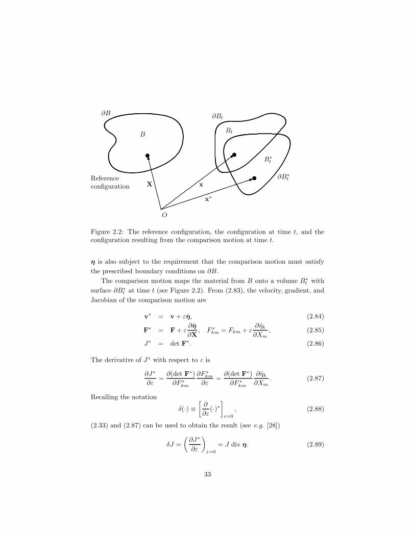
Figure 2.2: The reference configuration, the configuration at time t, and theconfiguration resulting from the comparison motion at time t.
η is also subject to the requirement that the comparison motion must satisfythe prescribed boundary conditions on ∂B.
The comparison motion maps the material from B onto a volume B∗t with
surface ∂B∗t at time t (see Figure 2.2). From (2.83), the velocity, gradient, and
Jacobian of the comparison motion are
v∗ = v + εη, (2.84)
F∗ = F + ε∂η
∂X, F ∗
km = Fkm + ε∂ηk
∂Xm, (2.85)
J∗ = det F∗. (2.86)
The derivative of J∗ with respect to ε is
∂J∗
∂ε=∂(det F∗)∂F ∗
km
∂F ∗km
∂ε=∂(det F∗)∂F ∗
km
∂ηk
∂Xm. (2.87)
Recalling the notation
δ(·) ≡[∂
∂ε(·)∗]
ε=0
, (2.88)
(2.33) and (2.87) can be used to obtain the result (see e.g. [28])
δJ =(∂J∗
∂ε
)
ε=0
= J div η. (2.89)
33

Therefore, J∗ can be written
J∗ = J(1 + ε div η) +O(ε2), (2.90)
where the notation O(ε2) means that |O(ε2)/ε| → 0 as ε → 0.The density of the comparison motion can be determined from the equation
of conservation of mass (2.66):
ρ∗ =ρR
J∗ . (2.91)
Substituting (2.90) into this equation results in the expression
ρ∗ = ρ(1 − ε div η) + O(ε2). (2.92)
In applications of Hamilton’s principle to a continuous medium, it is often con-venient to introduce a comparison field for the density in the form
ρ∗ = ρ(X, t) + εr(X, t). (2.93)
The preceding two equations show that, as a consequence of the equation ofconservation of mass, the scalar field r = −ρ div η+O(ε). However, the fields ηand r can be regarded as independent if the equation of conservation of massis introduced into Hamilton’s principle as a constraint (see the discussion ofconstraints in Section 1.2.2). In such cases, it will be assumed that r(X, t) is anarbitrary C1 scalar field on B × [t1, t2] such that r(X, t1) = 0 and r(X, t2) = 0.
The comparison motion maps a volume element dV of B onto a volumeelement dV ∗
t of B∗t at time t. Similarly, it maps a surface element dS of ∂B
onto a surface element dS∗t of ∂B∗
t at time t. The relations between these volumeand surface elements can be obtained from (2.64) and (2.71):
dV ∗t = J∗ dV, (2.94)
n∗dS∗t = J∗ (F∗)−t N dS. (2.95)
Here n∗ is the outward directed unit vector that is normal to ∂B∗t .
As described in Chapter 1, Hamilton’s principle is a postulate concerningthe mechanical behavior of a system. The equations of motion are derived fromthe postulate as necessary conditions. Two examples of the types of analysisinvolved in obtaining equations of motion from statements of Hamilton’s princi-ple for a continuous medium will be presented in the remainder of this section.The methods used are quite similar to those that were used in the case of asystem of particles.
34

In analogy with the kinetic energy of a particle, the kinetic energy of thematerial in an element of volume dVt of Bt is 1
2ρv · v dVt. Therefore the totalkinetic energy of the material occupying the volume Bt is
T =∫
Bt
12ρv · v dVt =
∫
B
12ρRv · v dV . (2.96)
Consider the integral of T with respect to time from t1 to t2:
I =∫ t2
t1
T dt =∫ t2
t1
∫
B
12ρRv · v dV dt. (2.97)
When it is expressed in terms of the comparison motion (2.83), this integralbecomes
I∗(ε) =∫ t2
t1
∫
B
12ρRv∗ · v∗ dV dt. (2.98)
Taking the derivative of this equation with respect to ε,
dI∗(ε)dε
=∫ t2
t1
∫
B
ρRv∗ · η dV dt, (2.99)
and setting ε = 0 yields[dI∗(ε)dε
]
ε=0
=∫ t2
t1
∫
B
ρRv · η dV dt. (2.100)
Integrating the expression on the right by parts with respect to time gives
∫ t2
t1
ρRv · η dt =[ρRv · η
]t2
t1
−∫ t2
t1
ρRa · η dt. (2.101)
Using this result and recalling that η vanishes at t1 and t2, (2.100) becomes[dI∗(ε)dε
]
ε=0
= −∫ t2
t1
∫
B
ρRa · η dV dt = −∫ t2
t1
∫
Bt
ρa · η dVt dt, (2.102)
so thatδT = −
∫
B
ρRa · δx dV = −∫
Bt
ρa · δx dVt, (2.103)
whereδx = η. (2.104)
Note from (2.83) that this definition of δx is consistent with the notation (2.88).As a second example, consider the integral
C =∫
B
π
(J − ρR
ρ
)dV =
∫
Bt
π
(1 − ρR
ρJ
)dVt. (2.105)
35
This expression is the form in which the equation of conservation of mass willbe introduced as a constraint in Hamilton’s principle for a continuous medium.The scalar field π(X, t), which is assumed to be C1 on B × [t1, t2], is a La-grange multiplier. Expressed in terms of the comparison motion (2.83) and thecomparison field (2.93), this integral becomes
C∗(ε) =∫
B
π
(J∗ − ρR
ρ∗
)dV . (2.106)
Taking the derivative of this equation with respect to ε, setting ε = 0, and using(2.89) to evaluate the derivative of the Jacobian yields
δC =∫
B
πJ
(div η +
r
ρ
)dV . (2.107)
By using the divergence theorem, this result can be written
δC =∫
∂Bt
πn · δx dSt +∫
Bt
(−grad π · δx +
π
ρδρ
)dVt, (2.108)
where δρ = r.
2.4 The Fundamental Lemmas
The fundamental lemma of the calculus of variations (see Section 1.1) is theresult required to obtain differential equations that apply locally (that is, at apoint) from a global (that is, expressed in terms of an integral over a volume)variational statement. In this section, extensions of the fundamental lemmaare presented that are appropriate for applications of Hamilton’s principle to acontinuous medium (see Gurtin [34], pp. 20, 244).
Lemma 1 Let W be an inner product space, and consider a C0 fieldf : B × [t1, t2] → W. If the equation
∫ t2
t1
∫
B
f ·w dV dt = 0 (2.109)
holds for every C∞ field w : B × [t1, t2] → W that vanishes at timet1, at time t2, and on ∂B, then f = o on B × [t1, t2].
Lemma 2 Suppose that ∂B consists of complementary regular sub-surfaces ∂B1 and ∂B2. Let W be an inner product space, and con-sider a function f : ∂B2 × [t1, t2] → W that is piecewise regular andcontinuous in time. If the equation
∫ t2
t1
∫
∂B2
f ·w dS dt = 0 (2.110)
36

holds for every C∞ field w : B × [t1, t2] → W that vanishes at timet1, at time t2, and on ∂B1, then f = o on ∂B2 × [t1, t2].
These lemmas are important not only because they are used in obtainingthe local forms of the equations of motion from Hamilton’s principle, but alsobecause they impose smoothness requirements on the fields describing the ma-terial. Both of these aspects were illustrated in the case of a system of particlesin Chapter 1.
Because these lemmas are so important, a proof of Lemma 1 given by Gurtin([34], p. 224) will be presented. The proof proceeds by assuming that the fieldf does not vanish at some point X0, t0 in B × (t1, t2), and then constructing asuitable field w such that (2.109) is violated.
Let ek be an orthonormal basis for W, so that f can be written f =fkek. Assume that fk(X0, t0) > 0 for some value of k and some point X0, t0
in B × (t1, t2). Let α be a positive scalar. Denote the open interval of time(t0 − α, t0 + α) by Tα, and denote the open region of space |X0 − X| < α byΩα. Because of the continuity of f , there is a value of α such that fk(X, t) > 0in Ωα × Tα. Define β(t) to be a scalar function on [t1, t2] that is C∞ and hasthe property that β(t) > 0 if t is in Tα and β(t) = 0 otherwise. Define γ(X) tobe a scalar field on B that is C∞ and has the property that γ(X) > 0 if X isin Ωα and γ(X) = 0 otherwise.7 Then define
w = β(t)γ(X)ek . (2.111)
The vector field w is C∞ on B× [t1, t2] and vanishes at time t1, at time t2, andon ∂B. It has been constructed so that
∫ t2
t1
∫
B
f ·w dV dt =∫
Tα
∫
Ωα
fkβ(t)γ(X) dV dt > 0, (2.112)
which violates (2.109). Therefore f must vanish in B × (t1, t2). Because thefield f is continuous on B × [t1, t2], it must vanish on B × [t1, t2].
Two minor variations of Lemmas 1 and 2 will also be used:
Lemma 3 Let the motion (2.51) be C2 on B × [t1, t2]. Let W be anIPS, and consider a C0 field f : B × [t1, t2] → W. If the equation
∫ t2
t1
∫
Bt
f ·w dVt dt = 0 (2.113)
holds for every C∞ field w : B × [t1, t2] → W that vanishes at timet1, at time t2, and on ∂B, then f (x, t) = o on B × [t1, t2].
7The existence of functions β(t) and γ(X) having these properties can be demonstrated(Gurtin [34], p. 19).
37
To prove this result, (2.113) can be written∫ t2
t1
∫
B
Jf ·w dV dt = 0. (2.114)
Because Jf is continuous on B × [t1, t2], Lemma 1 requires that Jf = o onB× [t1, t2]. Because J > 0, the function f (X, t) = o on B× [t1, t2], so f (x, t) = oon B × [t1, t2].
Lemma 4 The complementary regular subsurfaces ∂B1 and ∂B2 willbe mapped onto surfaces ∂Bt1 and ∂Bt2 by the motion (2.51). Let themotion (2.51) be C2 on B × [t1, t2]. Let φ(X, t) be a scalar functiondefined on ∂B2 × [t1, t2] that is piecewise regular and continuous intime. If the equation
∫ t2
t1
∫
∂Bt2
φn ·w dSt dt = 0 (2.115)
holds for every vector field w that is C∞ on B× [t1, t2] and vanishesat time t1, at time t2, and on ∂B1, then φ = 0 on ∂Bt2 × [t1, t2].
The proof is similar to that of Lemma 3. Equation (2.115) can be written
∫ t2
t1
∫
∂B2
φJF−tN ·w dS dt = 0. (2.116)
Because φJF−t is continuous on B × [t1, t2], φJF−tN is piecewise regularand continuous in time on ∂B2 × [t1, t2]. Therefore, Lemma 2 requires thatφJF−tN = o on ∂B2 × [t1, t2]. From (2.71), this implies that φ = 0 on∂B2 × [t1, t2].
38

Chapter 3
Mechanics of ContinuousMedia
Applications of Hamilton’s principle to deformable continuous media are dis-cussed in this chapter. Statements of the principle for continuous media areformally very similar to those for systems of particles, and certainly were mo-tivated by them. However, it should be emphasized that the statements forcontinuous media stand as independent postulates; they are not derived fromHamilton’s principle for a system of particles. It will be shown that the lo-cal forms of the equations of motion for continuous media and their associatedboundary conditions are obtained as necessary conditions implied by Hamilton’sprinciple. The classical theories of fluid and solid mechanics will be described,and also two recent theories of materials with microstructure. It will be shownthat postulates of Hamilton’s principle that have been introduced to obtainmore general theories are natural and well motivated extensions of the classicaltheories.
Problems in the mechanics of continuous media usually involve nonconserva-tive forces, and it is frequently convenient to include constraints in statementsof Hamilton’s principle. Therefore, the postulates that will be introduced inthis work will be expressed in the same form as the second form of Hamilton’sprinciple for a system of particles stated on page 19. They will be developedby the heuristic approach of identifying terms associated with the mechanics ofcontinuous media that are analogous to the terms that appear in (1.48). In oneexample that does not involve nonconservative forces, Hamilton’s principle willbe expressed in the first form stated on page 13.
39

3.1 The Classical Theories
In this section theories are discussed in which the mechanical behavior of amaterial is completely described by its motion
x = χ(X, t). (3.1)
Hamilton’s principle will be postulated for a finite amount of material thatoccupies a bounded regular region B in a prescribed reference configuration attime t1. As the material undergoes a motion (3.1), it will occupy a volume Bt
at each time t. Therefore Bt is called a material volume; it contains the samematerial at each time t.
Throughout this section an admissible motion will refer to a motion (3.1)of the material, from the prescribed reference configuration at time t1 to a pre-scribed configuration at time t2, that is C2 on B×[t1, t2] and satisfies prescribedboundary conditions on ∂B. A comparison motion will refer to an admissiblemotion
x∗ = χ(X, t) + εη(X, t), (3.2)
where η(X, t) is an arbitrary C2 vector field on B × [t1, t2] subject to the re-quirements that η(X, t1) = o and η(X, t2) = o.
3.1.1 Ideal Fluids
The terms ideal or inviscid fluid refer to a model of fluid behavior in which theeffects of viscosity are neglected. This is the simplest model for a continuousmedium. Two cases, compressible and incompressible fluids, will be treated.
Consider how one might postulate Hamilton’s principle for an ideal fluid ina form analogous to the first form for a system of particles stated on page 19.An admissible motion and comparison motion of the fluid are given by (3.1) and(3.2). It will be assumed that there is no geometrical constraint on the motionof the fluid on ∂B.
The density ρ(X, t) of the fluid will be assumed to be a C1 scalar field onB × [t1, t2]. In Section 2.3, an admissible comparison density field was definedby
ρ∗ = ρ(X, t) + εr(X, t), (3.3)
where r(X, t) is an arbitrary C1 scalar field on B × [t1, t2] subject to the re-quirements that r(X, t1) = 0 and r(X, t2) = 0.
Consider the individual terms in (1.48):
• The potential energy U If the fluid is compressible, it can store potentialenergy in the form of energy of deformation (in the same way energy is stored
40

in a deformed spring). The deformation of a fluid is expressed in terms of itschange in density from a reference state. Therefore, let it be assumed that thereis a scalar function of the density e(ρ), the internal energy, that is defined suchthat the potential energy of each element dVt of the fluid contained in Bt isρe(ρ) dVt. It will be assumed that the second derivative of the function e(ρ) ex-ists and is continuous. In modern terminology, the assumption that the internalenergy depends only on the density of the fluid is a constitutive assumption thatcharacterizes an elastic fluid. The total potential energy of the fluid containedin Bt is
U =∫
Bt
ρe(ρ) dVt. (3.4)
• The virtual work δW External forces acting on the fluid will be introducedby means of virtual work terms. Let there be a prescribed vector field b(X, t),the body force, that is C0 on B× [t1, t2] and defined such that the external forceexerted on a volume element dVt of the fluid contained in Bt is ρb dVt. Thisfield represents any external forces that are distributed over the volume of thefluid, such as its weight. The virtual work done by this force will be expressedin the form ρb dVt · δx, which is clearly analogous to (1.42). The virtual workdone on the fluid contained in Bt is
∫
Bt
ρb · δx dVt. (3.5)
It will also be assumed that there is a prescribed scalar field p0(X, t), the externalpressure, that is continuous in time and piecewise regular on ∂B × [t1, t2] anddefined such that the external force exerted on an area element dSt of ∂Bt is−p0n dSt. The resulting virtual work will be written −p0n dSt·δx, so the virtualwork on the fluid contained in Bt is
−∫
∂Bt
p0n · δx dSt. (3.6)
Therefore, the virtual work done on the fluid by external forces is postulated tobe of the form
δW =∫
Bt
ρb · δx dVt −∫
∂Bt
p0n · δx dSt. (3.7)
• The constraint C The motion of the fluid and its density field are relatedthrough the equation of conservation of mass. The comparison motion (3.2)and the comparison density field (3.3) can be regarded as independent if theequation of conservation of mass (2.66) is introduced into Hamilton’s principleas a constraint. The constraint will be written in the form
C =∫
Bt
π
(1 − ρR
ρJ
)dVt, (3.8)
41

where the unknown field π(X, t), which is assumed to be C1 on B × [t1, t2], isa Lagrange multiplier.• The kinetic energy T The kinetic energy of the fluid is
T =∫
Bt
12ρv · v dVt. (3.9)
Using these definitions, we can state Hamilton’s principle for an ideal fluid:
Among comparison motions (3.2) and comparison density fields (3.3),the actual motion and field are such that
∫ t2
t1
[δ(T − U ) + δW + δC]dt = 0. (3.10)
It was shown in Section 2.3 [Equations (2.103) and (2.108)] that the termsδT and δC can be written
δT = −∫
Bt
ρa · δx dVt, (3.11)
δC =∫
∂Bt
πn · δx dSt +∫
Bt
(−grad π · δx +
π
ρδρ
)dVt. (3.12)
The potential energy is
U =∫
Bt
ρe(ρ) dVt =∫
B
ρRe(ρ) dV . (3.13)
In terms of the comparison density field (3.3), this is
U∗ =∫
B
ρRe∗ dV , (3.14)
where e∗ = e(ρ∗). The derivative of this expression with respect to ε is
dU∗
dε=∫
B
ρRde∗
dρ∗∂ρ∗
∂εdV =
∫
B
ρRde∗
dρ∗r dV , (3.15)
so that the variation of the potential energy is
δU =∫
B
ρRde
dρδρ dV =
∫
Bt
ρde
dρδρ dVt. (3.16)
Upon substituting (3.7), (3.11), (3.12), and (3.16) into Equation (3.10), itcan be written
∫ t2
t1
[∫
Bt
(−ρa − grad π + ρb) · δx dVt +∫
Bt
(π
ρ− ρ
de
dρ
)δρ dVt
+∫
∂Bt
(π − p0)n · δx dSt
]dt = 0.
(3.17)
42
The equation of motion and boundary condition for the fluid can be deducedfrom this equation by applying Lemmas 3 and 4 of Section 2.4. Because thefields η = δx and r = δρ are arbitrary, it can be assumed that δρ = 0 onB × [t1, t2] and that δx = o on ∂B × [t1, t2]. As a result, the second and thirdintegrals in (3.17) vanish. Then applying Lemma 3 to the remaining integralyields the equation
ρa = −grad π + ρb on Bt × [t1, t2] . (3.18)
This is called the equation of balance of linear momentum. Next, assuming thatδx = o on B × [t1, t2] and applying Lemma 3 to (3.17) yields the equation
π = ρ2 de
dρon Bt × [t1, t2] . (3.19)
This equation determines the Lagrange multiplier π as a function of the den-sity of the fluid. Finally, applying Lemma 4 to (3.17) provides the boundarycondition
π = p0 on ∂Bt × [t1, t2] . (3.20)
A physical interpretation of the Lagrange multiplier π can be gained bywriting (3.17) in terms of a material volume of fluid B′
t that is contained withinBt (Figure 3.1):
∫ t2
t1
[ ∫
B′t
(−ρa − grad π + ρb) · δx dVt +∫
B′t
(π
ρ− ρ
de
dρ
)δρ dVt
+∫
∂B′t
(π − p)n · δx dSt
]dt = 0.
(3.21)
Here the term −pn is the normal traction exerted on the fluid within B′t by
the fluid exterior to B′t; that is, p is the pressure of the fluid. The function p
is not prescribed, but is a constitutive function that is assumed to be C1 onB × [t1, t2]. By the same procedure that was applied to (3.17), (3.21) impliesEquations (3.18) and (3.19) on B′
t × [t1, t2] and the boundary condition
π = p on ∂B′t × [t1, t2] . (3.22)
Thus the Lagrange multiplier π is the pressure of the fluid. Furthermore, observefrom (3.19) that Hamilton’s principle yields the constitutive equation for thepressure of the fluid in terms of the internal energy.
At this point, the usual method of determining the equation of motion foran ideal fluid will be sketched for the purpose of comparison with Hamilton’sprinciple. The approach used is to write a postulate for an arbitrary material
43

B′
∂B
∂B′B′
t
∂Bt
∂B′t
Figure 3.1: A volume of fluid B′ that is contained within B and the correspond-ing volume B′
t that is contained within Bt at time t.
volume of the fluid that is analogous to Newton’s second law for a system ofparticles (see e.g. Gurtin [35], pp. 105-110).
Let B′t be an arbitrary volume contained within Bt (Figure 3.1). The linear
momentum of an element dVt of B′t is the product of its mass and velocity,
ρv dVt. It is postulated that, at an arbitrary instant in time, the rate of changeof the total linear momentum of the fluid contained within B′
t is equal to thetotal external force exerted on the fluid:
d
dt
∫
B′t
ρv dVt =∫
B′t
ρb dVt −∫
∂B′t
pn dSt. (3.23)
As a consequence of the equation of conservation of mass and Reynolds’ trans-port theorem (see e.g. Gurtin [35], pp. 78-79),
d
dt
∫
B′t
ρv dVt =∫
B′t
ρa dVt. (3.24)
Using this result and the divergence theorem, (3.23) can be written∫
B′t
(ρa + grad p − ρb)dVt = 0. (3.25)
Because the volume B′t is arbitrary, this equation implies that
ρa = −grad p+ ρb on B × [t1, t2] . (3.26)
It is clear from this derivation why this equation is referred to as the balance oflinear momentum.
This direct method of obtaining the equation of balance of linear momen-tum is simpler than Hamilton’s principle, although if the derivation of Reynolds’transport theorem is regarded as an integral part of the process, the differenceis not so pronounced. Nevertheless, their relative complexity is a criticism thathas been made of variational methods in continuum mechanics. Note, however,
44

that the direct method does not yield (3.19). Other advantages of Hamilton’sprinciple, particularly in connection with its ability to incorporate constraints,will be illustrated in subsequent examples. The author regards direct and varia-tional methods as complementary, not competitive. In some cases one method ismore advantageous and in some the other, and often both methods lend insightto a given problem.
If the constitutive relation for the internal energy as a function of the densityis known, (2.70), (3.18), and (3.19) provide a system of equations with which todetermine the density field ρ, velocity field v, and pressure field π = p. Althoughthis is a simple theory, it is the one used in the study of aerodynamics to analyzehigh-speed flows except in regions (such as boundary layers and wakes) wherethe effects of viscosity cannot be neglected. In this application, (3.19) is usuallyassumed to be the isentropic relation
p
ργ= constant, (3.27)
where γ, the ratio of specific heats, is assumed to be constant. When it islinearized in terms of small perturbations, this theory is also used in the studyof the propagation of acoustic waves. Let
v = v, (3.28)
ρ = ρR + ρ, (3.29)
where v and ρ are small perturbations and the reference density ρR is assumedto be homogeneous. Using (3.27), (2.70) and (3.18) can be written (in theabsense of the body force)
∂ρ
∂t+ ρR div v = 0, (3.30)
ρR∂v∂t
+γpR
ρRgrad ρ = 0. (3.31)
Eliminating v from these two equations yields the linear wave equation
∂2ρ
∂t2= α2 52 ρ, (3.32)
where α =√γpR/ρR is the sound speed.
Thus far, the theory of a compressible ideal fluid has been discussed. If thefluid is assumed to be incompressible, ρ = ρR = constant. In this case, thereis no energy of deformation, so the potential energy U = 0. The equation ofconservation of mass (2.66) becomes J = 1, so the constraint (3.8) reduces to
C =∫
Bt
π
(1 − 1
J
)dVt. (3.33)
45

The other terms in (3.10) are unchanged. By using the same procedure as inthe case of a compressible fluid, (3.10) leads to the equation of balance of linearmomentum
ρa = −grad π + ρb on Bt × [t1, t2] (3.34)
and the boundary condition
π = p0 on ∂Bt × [t1, t2] . (3.35)
This equation of balance of linear momentum and boundary condition are iden-tical to those obtained in the case of a compressible fluid, but there is no equiv-alent to (3.19). The pressure π is not a constitutive function of the density. Foran incompressible fluid, the equation of conservation of mass (2.70) reduces to
div v = 0. (3.36)
Equations (3.34) and (3.36) provide two equations with which to determine thevelocity field v and pressure field π. The theory of incompressible ideal fluids isused in the study of hydraulics and in aerodynamics for the analysis of low-speedflows in regions where viscosity is not important.
Applications of Hamilton’s principle to ideal fluids are discussed by Eckart[24], Herivel [43], Lanczos [50], Leech [51], Serrin [65], and Taub [67].
3.1.2 Elastic Solids
An elastic solid can be characterized by the assumption that the internal energyis a function of the deformation gradient F, so that the potential energy of thematerial contained in Bt is
U =∫
Bt
ρe(F) dVt =∫
B
ρRe(F) dV . (3.37)
It will be assumed that the function e(F) is differentiable on a suitable opendomain of its argument and that DIV (∂e/∂F) is continuous on B × [t1, t2].
Suppose that the surface ∂B consists of complementary regular subsurfaces∂B1 and ∂B2, and that the motion of the material is prescribed on ∂B1. Letthere be no constraint on the motion of the material on ∂B2.
Let there be a prescribed vector field t0(x, t), the external traction, that isdefined on ∂Bt2 × [t1, t2] such that the external force exerted on an element dSt
of ∂Bt2 is t0 dSt. Then define a vector field s0(X, t) by s0 dS = t0 dSt, and lets0 be assumed to be continuous in time and piecewise regular on ∂B2 × [t1, t2].The virtual work done by the external traction is t0 dSt · δx = s0 dS · δx, and
46
the total virtual work done by external forces on the material contained in Bt
isδW =
∫
B
ρRb · δx dV +∫
∂B2
s0 · δx dS, (3.38)
where the body force b is defined as in the preceding subsection. Note that δxmust vanish on ∂B1 because the comparison motion (3.2) must satisfy the pre-scribed boundary conditions on ∂B.
The kinetic energy of the material contained in Bt is
T =∫
B
12ρRv · v dV . (3.39)
Hamilton’s principle for an elastic material states:
Among admissible comparison motions (3.2), the actual motion ofthe material is such that
∫ t2
t1
[δ(T − U ) + δW ] dt = 0. (3.40)
To determine the variation of the internal energy, it is first expressed in termsof the comparison motion:
U∗ =∫
B
ρRe(F∗) dV . (3.41)
The derivative of this expression with respect to ε is
∂U∗
∂ε=∫
B
ρRde∗
dF∗ · ∂F∗
∂εdV =
∫
B
ρRde∗
dF∗ · ∂η∂X
dV , (3.42)
where e∗ = e(F∗). In terms of components, this equation is
∂U∗
∂ε=∫
B
ρR∂e∗
∂F ∗km
∂F ∗km
∂εdV =
∫
B
ρR∂e∗
∂F ∗km
∂ηk
∂XmdV . (3.43)
Therefore, the variation of the potential energy is
δU =[∂U∗
∂ε
]
ε=0
=∫
B
S ·∂η
∂XdV , (3.44)
whereS = ρR
de
dF, Skm = ρR
∂e
∂Fkm. (3.45)
The linear transformation S is called the first Piola-Kirchoff stress. By meansof the divergence theorem, (3.44) can be written
δU =∫
∂B2
SN · δx dS −∫
B
DIV S · δx dV . (3.46)
47

Substituting this expression, (2.103), and (3.38) into Equation (3.40), it assumesthe form ∫ t2
t1
[∫
B
(−ρRa + DIV S + ρRb) · δx dV
+∫
∂B2
(s0 − SN) · δx dS]dt = 0.
(3.47)
Invoking Lemmas 1 and 2 of Section 2.4, this equation yields the equation ofbalance of linear momentum
ρRa = DIV S + ρRb on B × [t1, t2] (3.48)
and the boundary condition
SN = s0 on ∂B2 × [t1, t2] . (3.49)
When the constitutive relation e(F) is specified, (3.45) and (3.48) can beused to determine the displacement field u and the Piola-Kirchhoff stress S.The constitutive relations for elastic materials are discussed by Gurtin([34],Chapter C, [35], Chapters IX and X), Truesdell and Noll ([70], Chapters Cand D), and Truesdell and Toupin ([71], pp. 723-727). The linear theory ofelasticity is obtained by assuming that e is a quadratic form in the linear straintensor E,
ρRe = 12AijkmEijEkm, (3.50)
where the coefficients Aijkm are constants. If the material is isotropic, it can beshown that
Aijkm = λδijδkm + µ(δikδjm + δimδjk), (3.51)
where λ and µ are the Lame constants. In that case the constitutive equationfor the Piola-Kirchhoff stress is
S = λ(tr E)1 + 2µE, Skm = λEjjδkm + 2µEkm. (3.52)
By expressing the variation of the potential energy (3.44) as an integralover Bt, it can be written
δU =∫
Bt
T · ∂η∂x
dVt, (3.53)
where the Cauchy stress T is defined by
T =1J
SFt, Tkm =1JSkj
∂χm
∂Xj. (3.54)
48

By using the expression (3.53) for δU , (3.47) can be written∫ t2
t1
[∫
Bt
(−ρa + div T + ρb) · δx dVt
+∫
∂Bt2
(t0 −Tn) · δx dSt
]dt = 0,
(3.55)
which yields the equation of balance of linear momentum
ρa = div T + ρb on Bt × [t1, t2] (3.56)
and the boundary condition
Tn = t0 on ∂Bt2 × [t1, t2] . (3.57)
There are some elastic materials, of which rubber is the best known example,for which the assumption that the material is incompressible can be a useful ap-proximation. The equations governing an incompressible elastic material can beobtained by introducing the constraint (3.33) into Hamilton’s principle. Whenthe variation of (3.33) is included in (3.55), the resulting equation of balance oflinear momentum is
ρa = div (−π1 + T) + ρb on Bt × [t1, t2] (3.58)
and the boundary condition is
(−π1 + T)n = t0 on ∂Bt2 × [t1, t2] . (3.59)
In this case there is an additional governing equation, the constraint
J = 1, (3.60)
and an additional unknown field, the pressure π.If the external forces acting on an elastic material are conservative, Hamil-
ton’s principle can be stated in a manner analogous to the first form for a systemof particles on page 13 (see e.g. Washizu [73]). Suppose that there exist scalarfields ψb(x, t) and ψb(x, t) such that
b = −grad ψb, s0 = −grad ψs. (3.61)
Then Hamilton’s principle for an elastic material can be stated:
Among admissible motions, the actual motion of the material is suchthat the integral
I =∫ t2
t1
(T − U − Ue) dt (3.62)
is stationary in comparison with neighboring admissible motions.
49
The term Ue is defined by
Ue =∫
B
ρRψb dV +∫
∂B
ψs dS. (3.63)
In terms of the comparison motion, the integral (3.62) is
I∗(ε) =∫ t2
t1
(T ∗ − U∗ − U∗e ) dt, (3.64)
whereU∗
e =∫
B
ρRψ∗b dV +
∫
∂B
ψ∗s dS, (3.65)
ψ∗b = ψb(x∗, t), and ψ∗
s = ψs(x∗, t). The derivative of this expression withrespect to ε is
∂U∗e
∂ε=
∫
B
ρR∂ψ∗
b
∂x∗ · ∂x∗
∂εdV +
∫
∂B
∂ψ∗s
∂x∗ · ∂x∗
∂εdS
=∫
B
ρR∂ψ∗
b
∂x∗ · η dV +∫
∂B2
∂ψ∗s
∂x∗ · η dS,(3.66)
and, using (3.61), the value of this derivative when ε = 0 is[∂U∗
e
∂ε
]
ε=0
= −∫
B
ρRb · η dV −∫
∂B2
s0 · η dS. (3.67)
Therefore the first form of Hamilton’s principle for an elastic material impliesthat
[dI∗(ε)dε
]
ε=0
=∫ t2
t1
[−∫
B
ρRa · η dV +∫
B
DIV S · η dV
−∫
∂B2
SN · η dS +∫
B
ρRb · η dV
+∫
∂B2
s0 · η dS]dt = 0,
(3.68)
which is identical to (3.47).The application of Hamilton’s principle to elastic materials is discussed by
Gurtin ([34], pp. 223-226), Love ([53], Chapter VII), Washizu [73], and Wein-stock [74].
3.1.3 Inelastic Materials
The theories discussed in the preceding two subsections are very special due tothe assumptions that were made concerning the functional form of the internalenergy. Those assumptions restrict the application of the resulting equations,
50

a priori, to elastic materials. For dissipative media, such as viscous fluids,viscoelastic materials, or thermoelastic materials, a more general approach isnecessary.
Hamilton’s principle can be stated for an arbitrary continuous medium, re-stricted only by the assumption that it does not exhibit microstructural effects.In place of the variation of the internal energy, a virtual work term of the form
−∫
B
S · δF dV (3.69)
is introduced, where the linear tranformation S is a constitutive variable subjectonly to the requirement that S and DIV S be continuous on B × [t1, t2]. Noassumption is made concerning the dependence of S on the motion or deforma-tion of the material. It is only assumed that work is done when the deformationgradient of the material changes, and S is the associated generalized force. Anunderstanding of this point is essential to an appreciation of the applicability ofHamilton’s principle to continuum mechanics.
Let the virtual work done on the material contained in Bt be written
δW = −∫
B
S · δF dV +∫
B
ρRb · δx dV +∫
∂B
s0 · δx dS, (3.70)
where the fields b and s0 are defined as in the preceding two subsections. Itwill be assumed that there are no geometric constraints on the motion of thematerial on ∂Bt.
The kinetic energy of the material contained in Bt is
T =∫
B
12ρRv · v dV . (3.71)
Hamilton’s principle for an arbitrary continuous medium that does not ex-hibit microstructural effects states:
Among comparison motions (3.2), the actual motion of the materialis such that ∫ t2
t1
(δT + δW ) dt = 0. (3.72)
In terms of the comparison motion (3.2), the deformation gradient is
F∗ = F + ε∂η
∂X, (3.73)
so the variation of F is
δF =[∂F∗
∂ε
]
ε=0
=∂η
∂X. (3.74)
51

Using this expression and the divergence theorem, the virtual work (3.69) canbe written
−∫
B
S · δF dV = −∫
∂B
SN · δx dS +∫
B
DIV S · δx dV . (3.75)
Therefore, using the expressions (3.70), (3.71), and (3.75), Equation (3.72) canbe written in the form
∫ t2
t1
[∫
B
(−ρRa + DIV S + ρRb) · δx dV
+∫
∂B
(s0 − SN) · δx dS]dt = 0.
(3.76)
This equation is identical to Equation (3.47) for an elastic solid. It thereforeleads to the same equation of balance of linear momentum
ρRa = DIV S + ρRb on B × [t1, t2] (3.77)
and boundary condition
SN = s0 on ∂B × [t1, t2] . (3.78)
Alternatively, by using the definition of the Cauchy stress (3.54), (3.72) can bewritten ∫ t2
t1
[∫
Bt
(−ρa + div T + ρb) · δx dVt
+∫
∂Bt
(t0 − Tn) · δx dSt
]dt = 0,
(3.79)
which is identical to Equation (3.55) for an elastic solid and leads to the sameequation of balance of linear momentum
ρa = div T + ρb on Bt × [t1, t2] (3.80)
and boundary condition
Tn = t0 on ∂Bt × [t1, t2] . (3.81)
Although this statement of Hamilton’s principle leads to equations of balanceof linear momentum and boundary conditions that are formally identical tothose that were obtained in the case of an elastic solid, the crucial difference isthat in this case the linear transformations S and T are constitutive variables.Equations (3.77)–(3.81) apply to an arbitrary continuous medium, subject onlyto the restriction that the work done by internal forces as the result of a motion
52

of the material is of the form (3.69).1 However, S and T are no longer derivablefrom a potential energy, but must be prescribed through constitutive relations.2
Consider an arbitrary volume of materialB′ contained withinB (Figure 3.1).Let the heat flux q be a constitutive vector field that is C1 on B × [t1, t2] anddefined such that the rate at which heat is lost from the material within B′
t byconduction is ∫
∂B′t
q · n dSt. (3.82)
Let the external heat supply s be a prescribed scalar field that is C0 on B×[t1, t2]and defined such that the rate at which heat is added to the material within B′
t
by external sources (such as radiation) is∫
B′t
ρs dVt. (3.83)
The postulate of balance of energy for the material contained within B′t can be
written in the form (see e.g. Leigh [52])
d
dt
∫
B′t
ρe dVt =∫
B′t
T · L dVt −∫
∂B′t
q ·n dSt +∫
B′t
ρs dVt, (3.84)
where e is the internal energy and L = ∂v/∂x is the velocity gradient. Becausethe volume B′
t is arbitrary, this equation implies the differential equation
ρe = T · L− div q + ρs on ∂B × [t1, t2] , (3.85)
which is called the equation of balance of energy.It is easy to show that
∫
B′t
T ·L dVt =∫
B′S · F dV. (3.86)
This term of the energy balance postulate is called the mechanical workingterm. Observe the correspondence between the form of this term and that ofthe virtual work (3.69). It will be shown that this correspondence can be usedto motivate postulates of balance of energy when Hamilton’s principle is usedto derive more general theories of continua. Briefly, the mechanical workingterms in the balance of energy postulates are deduced from the forms of thevirtual work terms in Hamilton’s principle.3 This approach insures that the
1Theories in which this restriction is relaxed will be described in the next section.2Notice that, because S and DIV S must be continuous, the form of the constitutive
equation for S or T may impose a more stringent smoothness requirement on the motion ofthe material.
3See Drumheller and Bedford [22]. Similar procedures have been suggested by Ericksen [26]and Serrin ([65], p. 148).
53

forms of the equations of balance of linear momentum and balance of energyare mutually consistent.
Thermoelasticity is an example of a theory in which the equation of balanceof energy (3.85) is required (see e.g. Nowinski [55]). Let the absolute temperatureθ(X, t) be defined to be a non-negative scalar field that is C2 on stint. Athermoelastic material can be characterized by the constitutive relations ([55],Chapter 4)
T = T(F, θ, grad θ),e = e(F, θ, grad θ),q = q(F, θ, grad θ).
(3.87)
These constitutive relations together with (2.70), (3.80), and (3.85) provide asystem of equations with which to determine the density ρ, displacement u,temperature θ, Cauchy stress T, internal energy e, and heat flux q.
3.2 Theories with Microstructure
In the classical theories of fluid and solid mechanics, the mechanical behavior of amaterial is completely described by its motion (3.1). In a continuum theory withmicrostructure, new fields are introduced that are independent of the motionand describe mechanical properties of the material that the classical theories areunable to express. Hamilton’s principle is a useful technique for obtaining theequations that govern the new fields. In this work, two examples of theories ofthis type will be described, a theory of granular solids developed by Goodmanand Cowin [31] and a general theory of elastic solids with microstructure due toMindlin [54].
When postulates of Hamilton’s principle were first formulated for the clas-sical theories of fluid and solid mechanics, the results being sought were wellknown. The two examples presented in this section, and the material on mix-tures in the following chapter, show how natural extensions of those originalpostulates can be used to obtain new theories.
3.2.1 Granular Solids
The work of Goodman and Cowin provides an interesting and informative ex-ample of the use of Hamilton’s principle to derive a relatively simple model of amaterial with microstructure. Although they did not use Hamilton’s principlein developing their theory, it provides a natural and advantageous approach totheories of this type.
54

They proposed a continuum theory for application to materials consisting ofsolid grains with interstitial voids. They introduced a field φ(X, t), the volumefraction of the material, that is a measure of the volume occupied by the grainsper unit volume of the material. The volume fraction can vary independentlyof the motion (3.1) as a result of deformations and reorientations of the grains.Let it be assumed that the motion (3.1) and comparison motion (3.2) are C3
and that the volume fraction φ(X, t) is C2 on B× [t1, t2]. A comparison volumefraction will be defined by
φ∗ = φ(X, t) + εf(X, t), (3.88)
where f(X, t) is an arbitrary C2 scalar field on B × [t1, t2] that satisfies theconditions f(X, t1) = 0 and f(X, t2) = 0.
The virtual work done on the material by internal forces is postulated to be∫
B
[−S · δF + ρRg δφ− c · δ(GRAD φ)]dV . (3.89)
Comparing this expression to (3.69), the virtual work associated with an ordi-nary continuous medium is supplemented by two new terms which state thatwork is done when change occurs in the volume fraction and in the gradient ofthe volume fraction of the material. It will be assumed that the Piola-Kirchhoffstress S and DIV S are continuous on B × [t1, t2]. The scalar field g is a consti-tutive function that is assumed to be C0 on B× [t1, t2] and is called the intrinsicequilibrated body force. The vector field c is also a constitutive function and isassumed to be C1 on B × [t1, t2].
The virtual work done by external forces that are distributed over the volumeBt is assumed to be of the form
∫
Bt
(ρb · δx + ρl δφ) dVt. (3.90)
The prescribed body force b and the scalar field l are assumed to be continuouson B× [t1, t2]. The field l is a prescribed function called the external equilibratedbody force.
Suppose that the surface ∂B consists of complementary regular subsurfaces∂B1 and ∂B2, and that the motion of the material and the volume fraction areprescribed on the surface ∂B1. (See Section 2.4.) The virtual work done byforces distributed on ∂B2 is postulated in the form
∫
∂Bt2
(t0 · δx +H0δφ) dS. (3.91)
55
The prescribed external traction t0 and the prescribed scalar function H0 areassumed to be continuous in time and piecewise regular on ∂Bt2 × [t1, t2].
The total virtual work done on the material contained in Bt is therefore
δW =∫
B
[−S · δF + ρRg δφ− c · δ(GRAD φ)]dV
+∫
Bt
(ρb · δx + ρl δφ)dVt +∫
∂Bt2
(t0 · δx +H0δφ) dS.(3.92)
The kinetic energy of the material is written in the form
T =∫
Bt
(12ρv · v + 1
2ρkφ2
)dVt. (3.93)
In comparison to an ordinary continuous medium, an additional kinetic energyexpression is introduced which contains the square of the material derivative ofthe new independent field, the volume fraction. This term is the kinetic energyassociated with the local expansion and contraction of the grains, which canoccur independently of the motion (3.1). In general, the coefficient k must betreated as a constitutive function.4 For simplicity in this discussion, k will beassumed to be a constant.
Observe that the virtual work and kinetic energy expressions that have beendefined follow in a natural and systematic way once the new independent field,the volume fraction, was introduced. In addition to the usual kinetic energydue to the translational motion of the material, a new kinetic energy expressedin terms of the rate of change of the volume fraction was included. Similarly,it was assumed that work is done when the volume fraction and its gradientundergo changes.
Hamilton’s principle for a Goodman-Cowin material states:
Among comparison motions (3.1) and comparison volume fractionfields (3.88), the actual motion and volume fraction are such that
∫ t2
t1
(δT + δW ) dt = 0. (3.94)
Notice from (3.88) that
GRAD φ∗ =∂φ
∂X+ ε
∂f
∂X, (3.95)
so thatδ(GRAD φ) =
∂f
∂X. (3.96)
4See the related discussion in Section 4.4.
56

Therefore the third term in the first integral of the virtual work expression (3.92)can be written
∫
B
c · δ(GRAD φ) dV =∫
B
c · ∂f∂X
dV =∫
Bt
h · ∂F∂x
dVt, (3.97)
where the vector fieldh =
1J
Fc (3.98)
is called the equilibrated stress vector. By applying the divergence theorem,(3.97) can be expressed as
∫
B
c · δ(GRAD φ) dV =∫
∂B2
h · n δφ dS −∫
Bt
divh δφdVt, (3.99)
where δφ = f .The integral with respect to time of the second term in the kinetic energy
expression (3.93) is
T2 =∫ t2
t1
∫
Bt
12ρkφ
2 dVt dt =∫ t2
t1
∫
B
12ρRkφ
2 dV dt. (3.100)
In terms of the comparison volume fraction field (3.88), this is
T ∗2 =
∫ t2
t1
∫
B
12ρRk(φ∗)2 dV dt. (3.101)
The derivative of this expression with respect to ε is
dT ∗2
dε=∫ t2
t1
∫
B
ρRkφ∗ ∂φ
∗
∂εdV dt =
∫ t2
t1
∫
B
ρRkφ∗f dV dt. (3.102)
Integrating this equation by parts with respect to time and evaluating the resultwhen ε = 0 yields
δT2 = −∫ t2
t1
∫
B
ρRkφ δφ dV dt = −∫ t2
t1
∫
Bt
ρkφ δφ dVt dt. (3.103)
Using (3.99) and (3.103), and expressing the Piola-Kirchhoff stress S in termsof the Cauchy stress T through (3.54), (3.94) can be written
∫ t2
t1
∫
Bt
[(−ρa + div T + ρb) · δx
+(−ρkφ + div h + ρl + ρg)δφ]dVt
+∫
∂Bt2
[(t0 − Tn) · δx + (H0 − h · n)δφ
]dSt
dt = 0.
(3.104)
57

Due to the independence of the fields δx and δφ, Lemmas 3 and 4 of Section 2.4can be applied to (3.104) to obtain the differential equations
ρa = div T + ρb
ρkφ = div h + ρl + ρg
on Bt × [t1, t2] (3.105)
and the boundary conditions
Tn = t0
h · n = H0
on ∂Bt2 × [t1, t2] . (3.106)
When constitutive relations are specified for the Cauchy stress T, the equili-brated stress vector h, and the intrinsic equilibrated body force g, (2.70) and(3.105) can be used to determine the density ρ, velocity v, and volume fractionφ.
Equations (3.105) are identical, with minor changes in notation, to the equa-tions obtained by Goodman and Cowin ([31], Equations (4.7) and (4.10)). Al-though they did not use Hamilton’s principle to obtain these equations, theydid use a variational analysis of the static case [17] to motivate them.
This theory has been used to analyze flows of granular materials by Cowin [16],Nunziato et al. [57], and Passman et al. [63], and has been applied to the propa-gation of waves in granular materials by Cowin and Nunziato [18] and Nunziatoand Walsh [58].
Two general observations are illustrated by this example. First, Hamilton’sprinciple yields an equation for each independent field required to describe themechanical state of a material. The independent fields in this example arethe motion and the volume fraction. This characteristic of Hamilton’s principlemakes it particularly advantageous for application to materials with microstruc-ture. Second, the generalized forces that are introduced into Hamilton’s principleas virtual work terms must either be prescribed or must be specified through con-stitutive relations. In this example, b, l, t, and H0are prescribed, while T, g,and h are constitutive variables.
The approach described at the end of Section 3.1.3 can be used to postulatethe equation of balance of energy for a Goodman-Cowin material. Recall thecorrespondence between the virtual work (3.69) containing the Piola-Kirchhoffstress and the mechanical working term (3.86) that appears in the balance ofenergy postulate for an ordinary continuous medium. The virtual work done byinternal forces in this example is (3.89). The corresponding mechanical workingterm for an arbitrary volume B′ of Goodman-Cowin material is
∫
B′
(S · F− ρRg φ+ c · GRAD φ
)dV. (3.107)
58

Equating this expression to the rate of change of the internal energy e of thematerial within B′ and introducing the heat conduction terms (3.82) and (3.83),a postulate of balance of energy for a Goodman-Cowin material is
d
dt
∫
B′ρRe dV =
∫
B′S · F dV −
∫
B′t
ρgφ dVt
+∫
B′c · GRAD φ dV −
∫
∂B′q · n dSt
+∫
B′t
ρs dVt.
(3.108)
The resulting local form of the equation of balance of energy is
ρe = T · L− ρgφ + h · grad φ− div q + ρs. (3.109)
This result is identical to the equation obtained by Goodman and Cowin ([31],Equation (4.11)).
3.2.2 Elastic Solids with Microstructure
In the theory described in the previous subsection, a new independent scalarfield, the volume fraction, was introduced which provides limited informationon the local state of deformation and orientation of the grains in a granularmedium. Mindlin [54] used Hamilton’s principle to obtain a theory of linearelastic materials with microstructure that contains more extensive informationconcerning the local state of deformation and orientation of the material. Histheory provides a clear illustration of the potential of Hamilton’s principle forgenerating new theories of continuous media.
Mindlin associates with each point of the material a microelement. In thecase of a granular medium, a microelement could represent a typical grain of thematerial. The position vector X of a material point in the reference configurationis assumed to be the position of the center of mass of a microelement in thereference configuration. As the result of a motion (3.1) of the material, theposition of the center of mass of the microelement at time t is x. Let theposition vector of a material point of the microelement relative to its center ofmass in the reference configuration be Ξ. The position vector of this materialpoint relative to the center of mass at time t is denoted by ξ (Figure 3.2). Themicrodisplacement of the material point of the microelement is defined by
u = ξ − Ξ. (3.110)
It is then assumed that for each material point of the microelement,
u = ψtξ, (3.111)
59

where the linear transformation ψ(X, t) is called the microdeformation. Themicrodeformation is the new independent field of the theory. It describes thestate of strain of the microelement associated with each material point. Letψ(X, t) be C2 on B× [t1, t2], and define the microdeformation comparison fieldby
ψ∗ = ψ(X, t) + εR(X, t), (3.112)
where the linear transformation R is an arbitrary C2 field on B× [t1, t2] subjectto the conditions that R(X, t1) = 0 and R(X, t2) = 0.
Microelement
Referenceconfiguration
Configurationat time t
AA
AA
AA
AA
AAAK:
7CCCO
XXXXXXz
O
Ξ
X
ξ
x
Figure 3.2: A microelement in the reference configuration and at time t.
The strain measures of the theory are the usual linear strain E, the relativedeformation
γ =(∂u∂X
)t
−ψ, γkm =∂um
∂Xk− ψkm, (3.113)
where u is the usual displacement, and the microdeformation gradient
κ =∂ψ
∂X, κkmn =
∂ψkm
∂Xn. (3.114)
Mindlin developed a theory for an elastic material with microstructure byintroducing an internal energy e that is a function of the strain measures E, γ,and κ. The total potential energy of the material contained in Bt is written
U =∫
B
ρRe(E,γ,κ) dV . (3.115)
60

It will be assumed that the terms
τ = ρR∂e
∂E, τkm = ρR
∂e
∂Ekm,
σ = ρR∂e
∂γ, σkm = ρR
∂e
∂γkm,
µ = ρR∂e
∂κ, µkmn = ρR
∂e
∂κkmn,
(3.116)
exist and are continuous on suitable open domains of their arguments, and thatthe fields DIV τ , DIV σ, and DIV µ, where
(DIV µ)km =∂µkmn
∂Xn, (3.117)
are continuous on B × [t1, t2].It will be assumed that on the surface ∂B there are no geometrical constraints
on the motion of the material or on the value of the microdeformation ψ. Thevirtual work done by external forces is postulated in the form
δW =∫
B
ρR(b · δx + D · δψ) dV +∫
∂B
(s0 · δx + M0 · δψ) dS. (3.118)
The body force b and the linear transformation D are assumed to be prescribedand continuous on B × [t1, t2]. The field D is called the double force per unitmass. The surface traction s0 and the linear transformation M0 are also pre-scribed and are assumed to be continuous in time and piecewise regular on∂B × [t1, t2]. The field M0 is called the double force per unit area. Compare(3.118) to the virtual work expressions (3.89) and (3.91) used in the theory ofgranular materials due to Goodman and Cowin. In the latter theory, the sup-plementary independent field was a scalar, the volume fraction. In the presenttheory, the supplementary independent field is a linear transformation, the mi-crodeformation. Thus the present theory contains much more information aboutthe local motion and deformation of the microelements.
The kinetic energy of the material is postulated in the form
T =∫
B
(12ρRv · v + 1
6ρ′Rψ ·Qψ) dV , (3.119)
whereψ ·Qψ = Qijkmψijψkm. (3.120)
The scalar ρ′R and linear transformation Q are constants which are determinedby the distribution of mass within the microelement in the reference configu-ration. The second term in (3.119) is the kinetic energy associated with the
61

rotation and rate of deformation of the microelement. Compare (3.119) withthe expression (3.93) for a Goodman-Cowin material, in which the additionalkinetic energy term was due to the dilatational motion of the microelement.
Hamilton’s principle for a Mindlin material states:
Among comparison motions (3.2) and microdeformation comparisonfields (3.112), the actual fields are such that
∫ t2
t1
[δ(T − U ) + δW ] dt = 0. (3.121)
In terms of the comparison motion and the comparison microdeformation field,the potential energy (3.115) is
U =∫
B
ρRe(E∗,γ∗,κ∗) dV . (3.122)
The derivative of this expression with respect to ε is
∂U∗
∂ε=∫
B
(τ∗ · ∂E
∗
∂ε+ σ∗ · ∂γ
∗
∂ε+ µ∗ · ∂κ
∗
∂ε
)dV , (3.123)
whereµ∗ · ∂κ
∗
∂ε= µ∗
kmn
∂κ∗kmn
∂ε. (3.124)
The second term in (3.123) can be written∫
B
σ∗ · ∂γ∗
∂εdV =
∫
B
[(σt)∗ · ∂η
∂X− σ∗ ·R
]dV
=∫
∂B
(σt)∗N · η dS −∫
B
DIV (σt)∗ · η dV
−∫
B
σ∗ ·RdV .
(3.125)
By performing similar manipulations on the other terms in (3.123), the variationof the potential energy can be expressed as
δU =∫
∂B
τn · δx dS −∫
B
DIV τ · δx dV
+∫
∂B
σtN · δx dS −∫
B
DIV σt · δx dV
−∫
B
σ · δψ dV +∫
∂B
µN · δψ dS
−∫
B
DIV µ · δψ dV ,
(3.126)
62

where δψ = R and(µN)km = µkmnNn. (3.127)
The integral from t1 to t2 of the second term in the kinetic energy (3.119) is
I =∫ t2
t1
∫
B
16ρ
′Rψ ·Qψ dV dt. (3.128)
Expressing this equation in terms of the comparison microdeformation field andtaking the derivative with respect to ε yields
dI∗
dε=∫ t2
t1
∫
B
13ρ′RQψ
∗ · R dV dt. (3.129)
This equation can be integrated by parts to obtain
δI = −∫ t2
t1
∫
B
13ρ
′RQψ ·RdV dt. (3.130)
Using this equation together with the expressions (3.118) and (3.126), (3.121)can be written
∫ t2
t1
∫
B
[−ρRa + DIV(τ + σt) + ρRb] · δx dV
+∫
B
(−13ρ
′RQψ + σ + DIV µ + ρRD) · δψ dV
+∫
∂B
[s0 − (τ + σt)N] · δx dS
+∫
∂B
(M0 + µN) · δψ dSdt = 0.
(3.131)
Due to the independence of the fields δx and δψ, this equation yields the dif-ferential equations
ρRa = DIV(τ + σt) + ρRb13ρ
′RQψ = σ + DIV µ + ρRD
on B × [t1, t2] , (3.132)
and the boundary conditions
(τ + σt)N = s0
µN = M0
on ∂B × [t1, t2] . (3.133)
Thus, in addition to the equation of balance of linear momentum, Hamilton’sprinciple leads to an equation of motion for the microdeformation ψ. Noticethat the two equations of motion are coupled through the term σ. The fact that
63

this coupling is derived explicitly is one of the strengths of Hamilton’s principle.It would be difficult to simply postulate the equations (3.132).
When the consitutive equation for the internal energy e is specified, (3.116)and (3.132) can be used to determine the fields τ , σ, and µ, the displacementfield u, and the microdeformation field ψ. Mindlin [54] obtained a linear theoryby expressing the internal energy as a second order expansion in it argumentsand used the theory to analyze the propagation of harmonic waves.
64

Chapter 4
Mechanics of Mixtures
Blood is a mixture of a liquid, called the plasma, and particles, primarily ery-throcytes, or red cells. In an erythrocyte sedimentation test, a vertical tube ofanticoagulated blood is allowed to stand at rest. The cells, being slightly denserthan the plasma, settle to the bottom of the tube. The rate at which the uppercell boundary falls is a standard clinical test for disease. When a leak occursin the cooling system of a nuclear reactor (known as a loss of coolant accident,or LOCA), vapor bubbles appear in the suddenly depressurized coolant fluid,and the bubbly liquid flows rapidly toward the leak. It was the study of thesetwo very disparate phenomena that resulted in the applications of Hamilton’sprinciple to the continuum theory of mixtures described in this chapter.
When the volume fraction of one constituent of a binary mixture (i.e. the vol-ume occupied by that constituent per unit volume of the mixture) changes, thevolume fraction of the other constituent must adjust accordingly. This volumefraction constraint can be introduced into a postulate of Hamilton’s principlefor the mixture by the method of Lagrange multipliers. When a bubble of gasin a liquid expands or contracts, it induces a radial motion in the surroundingfluid. The inertia associated with this radial motion can be introduced intoHamilton’s principle by including, in addition to the kinetic energy of trans-lational motion of the constituents, a kinetic energy expressed in terms of therate of change of the density of the gas. These ideas suggested that Hamilton’sprinciple could be a useful method for deriving theories of mixtures.
65

4.1 Motions and Comparison Motions of a Mix-ture
4.1.1 Motions
Consider a mixture of two constituents (a binary mixture), such as a fluid con-taining a distribution of particles or bubbles, or a porous solid saturated bya fluid. In general, the two constituents of the mixture can flow relative toone another. Their individual motions can be described by modeling the con-stituents as two superimposed continuous media. Let the symbol Cξ denote theξth constituent. A motion of Cξ is the vector field
x = χξ(Xξ, t), (4.1)
where x is the position vector at time t of the material point of Cξ whose positionvector is Xξ in a prescribed reference configuration.1 The inverse motion of Cξ
isXξ = χ−1
ξ (x, t). (4.2)
Consider a finite amount of the mixture that occupies a bounded regularregion B in a prescribed reference configuration at time t1. In general, theindividual motions (4.1) would cause the constituents to occupy different regionsat time t. To prevent the constituents from moving apart during the timeinterval [t1, t2], it will be assumed that the displacement of each constituentvanishes on ∂B, or, in the case of an ideal fluid constituent, it will be assumedthat the normal component of the velocity vanishes on ∂B. This is equivalentto assuming that the mixture is bounded by a rigid wall.2 As a result, bothconstituents occupy a single volume Bt = B with a single surface ∂Bt = ∂B
at each time t. This assumption is not merely a theoretical convenience. At afree surface of the mixture, the constituents could actually separate as shown inFigure 4.1. Then two types of surface result, a free surface of a single constituent,and a surface that is a boundary of one constituent but not of the other. Asystematic study of boundary conditions at the latter type of surface would bepossible using the methods to be described in Chapter 5.
Throughout this chapter the motions 4.1 will be assumed to be C3 onB × [t1, t2]. The description of the kinematics and deformation of Cξ in terms
1See the discussion of the motion of a continuous medium in Section 2.2.2An alternative approach would be to express Hamilton’s principle in terms of a fixed
spatial volume through which the constituents are allowed to diffuse. However, Leech [51]observes that “Many investigators.. . have tried to derive by applicationof Hamilton’s principlethe momentum equation using the so-called Eulerian coordinate system. They have appliedthe principle using a fixed (control) volume. This is not Hamilton’s principle, which for acontinuum must be associated with a fixed aggregate or control mass.”
66

Figure 4.1: Two constituents diffusing relative to one another at the boundaries.
of its motion is identical to that for a single continuous medium presented inSection 2.2. The velocity, acceleration, deformation gradient, Jacobian, dis-placement, and linear strain of Cξ are defined by
vξ =∂
∂tχξ(Xξ , t),
aξ =∂2
∂t2χξ(Xξ, t),
Fξ =∂
∂Xξχξ(Xξ, t),
Jξ = det Fξ,
uξ = χξ(Xξ, t) − Xξ,
Eξ =12
[∂uξ
∂Xξ+(∂uξ
∂Xξ
)t].
(4.3)
The material derivative of a field fξ(Xξ , t) is defined by
fξ =∂
∂tfξ(Xξ, t) =
∂
∂tfξ. (4.4)
67

The inverse motion (4.2) maps an element dVt ofBt at time t onto an elementdVξ in the reference configuration. These volume elements are related by (see(2.64))
dVt = JξdVξ. (4.5)
Let the part of dVt occupied by the constituent Cξ be dVξt, and let the mass of Cξ
contained in dVξt be dmξ. The partial density of Cξ is defined by ρξ = dmξ/dVt.The material density of Cξ is defined by ρξ = dmξ/dVξt, and the volume fractionof Cξ is defined by φξ = dVξt/dVt. Therefore
ρξ = φξρξ. (4.6)
The partial density ρξ is the mass of Cξ per unit volume of the mixture at time t.The material density ρξ is the mass of Cξ per unit volume of Cξ at time t, andthe volume fraction φξ is the volume of Cξ per unit volume of the mixture attime t. The fields ρξ(Xξ , t), ρξ(Xξ, t), and φξ(Xξ , t) will be assumed to be C2
on B × [t1, t2].One form of the equation of conservation of mass for Cξ is
Jξ =ρξR
ρξ=φξRρξR
φξρξ, (4.7)
where ρξR = ρξ(Xξ, t1), φξR = φξ(Xξ, t1), and ρξR = ρξ(Xξ, t1) are the valuesof the partial density, volume fraction, and material density in the referenceconfiguration. The equation of conservation of mass for Cξ can also be expressedin the form
ρξ + ρξ div vξ = 0. (4.8)
In this work, consideration will be limited to mixtures for which∑
ξ
φξ(x, t) = 1, (4.9)
where the notation∑
ξ
denotes summation over the constituents of the mixture.
That is, it will be assumed that the constituents of the mixture occupy all ofthe volume Bt at eact time t; there are no voids. Equation (4.9) is called thevolume fraction constraint. It plays a central role in the theories to be discussedin this chapter.
4.1.2 Comparison Fields
A motion (4.1) of Cξ will be called admissible if it is C3 on B × [t1, t2] and itsatisfies the prescribed boundary condition on ∂B. An admissible comparison
68

motion of Cξ is defined in analogy with (2.83),
x∗ξ = χξ(Xξ, t) + εηξ(Xξ, t)
= Kξ(Xξ , t, ε),(4.10)
where ε is a parameter and ηξ(Xξ , t) is an arbitrary C3 vector field on B×[t1, t2]subject to the conditions that ηξ(Xξ, t1) = o, ηξ(Xξ, t2) = o, and (4.10) satisfiesthe prescribed boundary condition on ∂B. The inverse of the comparison motionis
Xξ = K−1ξ (x∗
ξ , t, ε). (4.11)
The inverse motion gives the position vector in the reference configuration ofthe material point of Cξ whose position is x∗
ξ at time t.In addition to the comparison motion, comparison material density and com-
parison volume fraction fields are defined by
ρ∗ξ = ρξ(Xξ , t) + εrξ(Xξ , t),
φ∗ξ = φξ(Xξ , t) + εfξ(Xξ, t),
(4.12)
where rξ(Xξ, t) and fξ(Xξ, t) are arbitrary fields subject to the conditions thatthey are C2 on B × [t1, t2] and vanish at times t1 and t2.
Let the volume fraction of Cξ by expressed as a function of Xξ , t:
φξ = φξ(Xξ , t). (4.13)
Using this expression and the inverse motion (4.2), the volume fraction con-straint (4.9) can be written
∑
ξ
φξ(χ−1ξ (x, t), t) = 1. (4.14)
This equation can be written in terms of the inverse of the comparison motion(4.11) and the comparison volume fraction field (4.12)1 to obtain the relation
∑
ξ
φ∗ξ(K
−1ξ (x, t, ε), t, ε) = 1. (4.15)
The derivative of this equation with respect to ε is
∑
ξ
(∂φ∗
ξ
∂K−1ξ
·∂K−1
ξ
∂ε+∂φ∗
ξ
∂ε
)= 0. (4.16)
To evaluate the partial derivative of K−1ξ with respect to ε that appears in this
expression, the differential of (4.11) can be taken while holding Xξ and t fixedto obtain
o =∂K−1
ξ
∂x∗ξ
dx∗ξ +
∂K−1ξ
∂εdε. (4.17)
69

Therefore∂K−1
ξ
∂ε= −
∂K−1ξ
∂x∗ξ
[dx∗
ξ
dε
]
Xξ,t
= −∂K−1
ξ
∂x∗ξ
ηξ. (4.18)
Substituting this result into (4.16) and evaluating the resulting equation whenε = 0, one obtains [5]
∑
ξ
(grad φξ · δxξ − δφξ) = 0, (4.19)
where δxξ = ηξ and δφξ = fξ . Equation (4.19) is a constraint imposed on thevariations δxξ and δφξ by the volume fraction constraint. It will be introducedinto statements of Hamilton’s principle for mixtures in the form
∫
Bt
λ∑
ξ
(grad φξ · δxξ − δφξ) dVt = 0, (4.20)
where the scalar field λ(x, t) is a Lagrange multiplier that is assumed to be C1
on Bt × [t1, t2].The equations of conservation of mass of the constituents (4.7) will also be
introduced as constraints into statements of Hamilton’s principle for mixtures,in the same form as in the case of a single continuous medium (see (2.105)):
∑
ξ
∫
Bt
πξ
(1 − φξRρξR
φξρξJξ
)dVt
=∑
ξ
∫
B
πξ
(Jξ −
φξRρξR
φξρξ
)dV ,
(4.21)
where the scalar fields πξ(Xξ, t) are Lagrange multipliers that are assumed tobe C1 on B × [t1, t2]. To determine the variation of this expression, it can bewritten in terms of the comparison motion (4.10) and the comparison fields(4.12):
∑
ξ
∫
B
πξ
(J∗
ξ − φξRρξR
φ∗ξ ρ
∗ξ
)dV . (4.22)
Taking the derivative with respect to ε and setting ε = 0 yields
∑
ξ
∫
B
πξJξ
(div ηξ +
fξ
φξ+rξ
ρξ
)dV
=∑
ξ
∫
Bt
[−grad πξ · δxξ + πξ
(δφξ
φξ+δρξ
ρξ
)]dVt
(4.23)
where δρξ = rξ.
70

The postulates of Hamilton’s principle for mixtures that will be introducedin the following sections are closely analogous to those for a single material de-scribed in Chapter 3. The volume fraction constraint is a new element, and newdegrees of freedom will be seen to arise in comparison with the theories of sin-gle materials without microstructure. The formulations for mixtures have someelements in common with the theory for granular solids discussed in Section 3.2.
4.2 Mixtures of Ideal Fluids
4.2.1 Compressible Fluids
It will be assumed that each constituent Cξ has an internal energy per unit masseξ(ρξ) that is a function only of the material density of that constituent.3 Thesecond derivatives of these functions are assumed to be continuous. The totalpotential energy of the mixture contained in Bt is assumed to be the sum of thepotential energies of the constituents:
U =∑
ξ
∫
Bt
ρξeξ(ρξ) dVt. (4.24)
The virtual work done on the mixture by external forces is postulated in theform
δW =∑
ξ
∫
Bt
(ρξbξ + dξ) · δx dVt. (4.25)
In this expression the external force on each constituent is decomposed into twoparts. The body force bξ is the force per unit mass exerted on Cξ by externalagencies, such as gravity. It is assumed to be prescribed. The interaction force,or drag dξ is the force per unit volume exerted on Cξ by the other constituentof the mixture.4 The vector fields bξ(Xξ, t) and dξ(Xξ, t) will be assumed tobe C0 on B × [t1, t2]. Recall that the mixture is assumed to be bounded by arigid wall. As a result, no virtual work is done by external forces at the surface∂Bt.
The comparison fields (4.10) and (4.12) are subject to the constraints (4.20)and (4.23) arising from the volume fraction constraint and the equations of
3This assumption, like the assumptions made in Section 3.1 that led to theories of elasticfluids and elastic solids, will obviously result in a very special theory.
4Although the constituents are here being treated as inviscid with regard to their macro-scopic behavior, it is nevertheless assumed that they may exert drag forces on one another.This is a common assumption in mixture theories for processes in which macroscopic viscouseffects may be neglected (see e.g. Bowen [13].
71
conservation of mass. Therefore, the constraint term
δC =∑
ξ
∫
Bt
λ(grad φξ · δxξ − δφξ) dVt
+∑
ξ
∫
Bt
[−grad πξ · δxξ + πξ
(δφξ
φξ+δρξ
ρξ
)]dVt
(4.26)
will be included in Hamilton’s principle.The total kinetic energy of the mixture in Bt will be assumed to be the sum
of the kinetic energies due to the translational motions of the constituents:
T =∑
ξ
∫
Bt
12ρξvξ · vξ dVt. (4.27)
Based on the expressions (4.24)-(4.27), a postulate of Hamilton’s principlefor a mixture of elastic ideal fluids states [5]:
Among comparison motions (4.10) and comparison fields (4.12), theactual fields are such that
∫ t2
t1
[δ(T − U ) + δC + δW ]dt = 0. (4.28)
Substituting (4.24)-(4.27), this equation can be written
∑
ξ
∫ t2
t1
∫
Bt
[(−ρξaξ + ρξbξ + dξ − grad πξ + λ grad φξ) · δx
+(−ρξ
deξ
dρξ+πξ
ρξ
)δρξ +
(πξ
φξ− λ
)δφξ
]dVt dt = 0.
(4.29)
Because of the independence of the fields δxξ, δρξ, and δφξ for each constituent,Lemma 3 of Section 2.4 can be applied to (4.29) to obtain the equations
ρξaξ = ρξbξ + dξ − grad πξ + λ grad φξ,
πξ = φξρ2ξ
deξ
dρξ,
πξ = φξλ
on Bt × [t1, t2] . (4.30)
When constitutive relations are specified for the internal energies eξ(ρξ) and thedrag terms dξ, the three equations (4.30) together with (4.6), (4.8), and (4.9)can be used to determine the fields ρξ , ρξ , φξ, λ, vξ, and πξ.
Notice from (3.19) and the discussion following it that the term ρ2ξdeξ/dρξ
is the pressure of the constituent Cξ. From (4.30),
λ = ρ2ξ
deξ
dρξ. (4.31)
72

Thus a consequence of this postulate of Hamilton’s principle for a mixture is thatthe pressures of the constituents are equal. This condition is often introduced asan assumption in theoretical studies of multiphase flow. Models for mixtures inwhich this condition does not hold will be discussed later in this section. Also,observe that (4.30)1 can be written
ρξaξ = ρξbξ + dξ − φξ grad λ. (4.32)
The form of the last term in this equation has been a subject of some contro-versy among those interested in theoretical models for mixtures. The form thatappears here is a consequence of including the volume fraction constraint inHamilton’s principle.5
4.2.2 Incompressible Fluids
If both constituents of a binary mixture are incompressible (ρξ = ρξR = constant),(4.28) assumes the form
∫ t2
t1
(δT + δC + δW ) dt = 0. (4.33)
Equations (4.25) and (4.27) for δW and T are unchanged. The only change inEquation (4.26) for δC is that δρξ = 0. The equations resulting from Hamilton’sprinciple are
ρξaξ = ρξbξ + dξ − grad πξ + λ grad φξ,
πξ = φξλ
on Bt × [t1, t2] . (4.34)
Eliminating the Lagrange multipliers πξ yields the equations of balance of linearmomentum
ρξaξ = ρξbξ + dξ − φξ grad λ. (4.35)
For incompressible constituents, the equations of conservation of mass (4.8) canbe written
φξ + φξ div vξ = 0. (4.36)
If constitutive relations are specified for the drag terms dξ, the equations (4.9),(4.35), and (4.36) can be used to determine the fields λ, vξ , and φξ. TheLagrange multiplier λ is the pressure of the constituents.
The statement of Hamilton’s principle for a granular solid described in Sec-tion 3.2.1 contained a virtual work term expressed in terms of the variation of
5The comments in this paragraph have been discussed at length by Bedford andDrumheller [7].
73

the volume fraction of the material. Would the physics of the problem justifythe inclusion of such terms in a theory for a mixture of ideal fluids? Supposethat the theory is used to model a fluid containing a distribution of particles. Ifthe particles are sufficiently small, they will undergo mutual impacts as a resultof their Brownian motions. This diffusive effect of particle impacts is analogousto the ordinary pressure which arises in a fluid due to impacts on the molecularscale. The particles can also exert forces on one another through hydrodynamicinteractions when the mixture is in motion. Either of these phenomena willresult in work being done when the volume fraction of the particles changes.
The postulates of Hamilton’s principle that have been stated for a mixtureof ideal fluids can be extended to the case of a mixture of ideal fluids withdiffusivity by adding to (4.25) a virtual work term of the form [47]6
−∑
ξ
∫
Bt
Pξδφξ
φξdVt. (4.37)
In the case of incompressible constituents, the equations resulting from Hamil-ton’s principle are
ρξaξ = ρξbξ + dξ − grad πξ + λ grad φξ,
πξ = φξλ+ Pξ
on Bt × [t1, t2] . (4.38)
Eliminating the Lagrange multipliers λ results in the equations of balance oflinear momentum
ρξaξ = ρξbξ + dξ − φξ grad λ− grad Pξ. (4.39)
In addition to the gradient of the pressure λ appearing in the equations ofmotion, the gradients of the diffusive pressures Pξ also appear.
To apply this theory to the sedimentation of a distribution of rigid particlesin an incompressible fluid, Hill et al. [47] postulated the constitutive relations
dξ = dξ(φξ,vξ − vγ),
Pξ = Pξ(φξ,vξ − vγ),(4.40)
where ξ 6= γ. Notice that because the volume fractions are related through thevolume fraction constraint, it is not necessary to assume that the constitutiverelations are functions of both volume fractions. Hill et al. further assumed
6The generalized force in this expression is written in the form Pξ/φξ because it results insimpler equations. This does not imply an a priori assumption of the functional form of thediffusive force, because the terms Pξ are assumed to be constitutive functions of the volumefractions.
74

that these constitutive relations are isotropic and linear in the relative velocity,which implies that they must be of the forms
dξ = αξ(vξ − vγ),
Pξ = βξ ,(4.41)
where αξ and βξ are scalar functions of φξ.For purposes of comparison with this derivation, equivalent theories have
been derived by two other approaches. Craine [19] used postulated equationsof motion and introduced the volume fraction constraint into the second law ofthermodynamics (the Clausius-Duhem inequality) for the mixture. Drew [20]used an averaging approach.
Equations (4.9), (4.36), (4.39), and (4.41) have been applied to the erythro-cyte sedimentation test described in the introduction to this chapter by Hilland Bedford [46] and Hill et al. [47]. Figures 4.2 and 4.3 compare their numer-ical solutions to experimental measurements made using anticoagulated humanwhole blood by Whelan et al. [75]. In Figure 4.2, the predicted distributionof the cell volume fraction as a function of height in the vertical tube is com-pared to measurements made at several times. An empirical expression for the“drag coefficient” αξ was used, and the constitutive coefficients were chosen toobtain the best agreement with the data at 2 hours. The coefficients were thenheld fixed while the computations were extended to 4 hours and 8.5 hours. InFigure 4.3, the predicted position of the upper cell boundary as a function oftime, which is used as a clinical indicator of disease, is compared to the observedposition.
This theory has also been used to study the stability of steady sedimenta-tion of a uniform distribution of particles in a fluid by Hill [44] and Hill andBedford [45].
4.2.3 Fluids with Microinertia
Suppose that there is a spherical bubble of gas in an unbounded incompressibleliquid. Let the radius of the bubble be R, and let the densities of the gas and theliquid be ρg and ρf . If the bubble expands or contracts, it will induce a radialvelocity distribution in the liquid. The velocity of the liquid at a distance rfrom the center of the bubble is
vf =R2
r2R, (4.42)
75

0 0.2 0.4 0.6 0.8Cell concentration φ
0
4
8
12
16
20
Height (cm)
ue∆
Experiment, 2.0 hrExperiment, 4.0 hrExperiment, 8.5 hrTheory
∆∆
∆∆∆
∆∆∆
∆∆∆∆
eeeeee
eeeeee
ee
uuuuuuuuuuuuuu
uuuu
Figure 4.2: Comparison of the mixture theory with cell concentration profilesmeasured in blood sedimentation.
where the dot denotes the derivative with respect to time. The resulting kineticenergy of the liquid surrounding the bubble is
∫ ∞
R
12ρf 4πr2v2
f dr. (4.43)
Substituting the velocity distribution (4.42), this integral can be evaluated toobtain
2πρfR3R2. (4.44)
Because the mass of the gas within the bubble, (4/3)πR3ρg , is constant, thekinetic energy (4.44) can be expressed in terms of the rate of change of the gasdensity: (
2πρf ρ5/3gR R5
R
9ρ 11/3g
)˙ρ 2g , (4.45)
where ρgR and RR are reference values.
76

0 2 4 6 8 10Time (hr)
0
4
8
12
16
20
Height (cm) e ExperimentTheory
e e e e e e e e
Figure 4.3: Comparison of the mixture theory with the upper cell interfacemeasured in blood sedimentation.
Now consider a liquid containing a dilute distribution of bubbles, and sup-pose that in a prescribed reference configuration the bubbles are uniformly dis-tributed and each has radius RR and density ρgR. In a motion of this bubbleliquid, the bubbles will undergo volumetric oscillations and induce local radialmotions of the liquid. If it is assumed that the kinetic energy of the liquid sur-rounding each bubble can be approximated by the expression (4.45), the kineticenergy per unit volume of the mixture due to radial motions of the bubbles canbe obtained by multiplying (4.45) by the number of bubbles per unit volume.The number of bubbles per unit volume is φg/(4/3)πR3, where φg is the volumefraction of the gas. The product of this expression with (4.45) can be written
ρg
(ρf ρ
2/3gR R2
R
6ρ 11/3g
)˙ρ2g . (4.46)
77

This microkinetic energy due to bubble oscillations can have a dominant effecton the dynamic behavior of bubbly liquids (see van Wijngaarden [72]). Theequations governing the motion of a bubbly liquid can be obtained by introduc-ing the microkinetic energy into Hamilton’s principle [21].
For simplicity in this presentation, the relative motion between the bubblesand the liquid will be neglected. This is an acceptable assumption in manyapplications because of the relatively small mass of the bubbles. Thus themixture will be assumed to have a single motion (3.1). The microkinetic energyof the mixture contained in Bt will be expressed in the form
Tm =∫
Bt
12ρgIg(ργ ) ˙ρ2
g dVt =∫
B
12ρgRIg(ργ) ˙ρ2
g dV (4.47)
The term Ig(ργ ) is a constitutive function that depends on each of the con-stituent densities. This expression for the microkinetic energy is motivated by(4.46) and includes it as a special case. The integral of (4.47) with respect totime from t1 to t2 is
I =∫ t2
t1
Tm dt =∫ t2
t1
∫
B
12ρgRIg(ργ ) ˙ρ2
g dV dt. (4.48)
Proceeding in the now familiar way to determine the variation, this equation iswritten in terms of the comparison material density field (4.12)1 to obtain
I∗(ε) =∫ t2
t1
∫
B
12ρgRIg(ρ∗γ )( ˙ρ∗g)
2 dV dt. (4.49)
The derivative of this equation with respect to ε is
dI∗(ε)dε
=∫ t2
t1
∫
B
[ρgRI
∗g˙ρ∗g ˙rg + 1
2ρgR
(∑
γ
∂I∗g∂ρ∗γ
rγ
)( ˙ρ∗g)
2
]dV dt, (4.50)
where I∗g = Ig(ρ∗γ ). Integrating the first term by parts with respect to time andsetting ε = 0 yields the variation
δTm =∫
Bt
[−ρg
˙Ig ˙ρgδρg + 1
2ρg
(∑
γ
∂Ig∂ργ
δργ
)˙ρ2g
]dVt. (4.51)
The total kinetic energy of the mixture contained in Bt is
T =∫
Bt
[12ρv · v + 1
2ρgIg(ργ ) ˙ρ2g
]dVt, (4.52)
where ρ = ρf + ρg is the density of the mixture.
78

The potential energy of the mixture is postulated to be the total internalenergy for a mixture of two compressible ideal fluids:
U =∑
ξ
∫
Bt
ρξeξ(ρξ) dVt. (4.53)
Because there is not relative motion between the constituents, no work isdone by drag forces and the only virtual word done is that due to the externalbody force:
δW =∫
Bt
ρb · δx dVt. (4.54)
The constraint arising from the equations of balance of mass and the volumefraction constraint, (4.26), is altered only by the fact that there is a singlemotion:
δC =∑
ξ
∫
Bt
λ(grad φξ · δx − δφξ) dVt
+∑
ξ
∫
Bt
[−grad πξ · δx + πξ
(δφξ
φξ+δρξ
ρξ
)]dVt.
(4.55)
Based on (4.52)-(4.55), a statement of Hamilton’s principle for an ideal com-pressible liquid containing a distribution of bubbles of an ideal gas is [23]:
Among comparison motions (3.2) and comparison fields (4.12), theactual fields are such that
[t1, t2] [δ(T − U ) + δC + δW ] = 0. (4.56)
Substituting (4.52)-(4.55) and using the result (4.51), (4.56) can be written
∫ t2
t1
∫
Bt
[−ρa + ρb− grad (πf + πg)] · δx
+(−ρg
˙Ig ˙ρg + 1
2ρg∂Ig∂ρg
˙ρ2g − ρg
deg
dρg+πg
ρg
)δρg
+(
12ρg
∂Ig∂ρf
˙ρ2g − ρf
def
dρf+πf
ρf
)δρf
+(πg
φg− λ
)δφg +
(πf
φf− λ
)δφf
dVt dt = 0,
(4.57)
79

which yields the equations
ρa = ρb− grad (πf + πg),
ρg˙
Ig ˙ρg − 12ρg
∂Ig∂ρg
˙ρ2g = −ρg
deg
dρg+πg
ρg,
−12ρg
∂Ig∂ρf
˙ρ2g = −ρf
def
dρf+πf
ρf,
πg = φgλ,
πf = φfλ
on B × [t1, t2] . (4.58)
The last two equations can be used to eliminate the Lagrange multipliers πf
and πg, resulting in the three equations
ρa = ρb− grad λ,
ρ2g
˙Ig ˙ρg − 1
2ρg
(ρg∂Ig∂ρg
− φg
φfρf∂Ig∂ρf
)˙ρ2g = pf − pg,
λ = pf − 12ρgφf
φfρf∂Ig∂ρf
˙ρ2g,
(4.59)
where the constituent pressures pξ are
pξ = ρ2ξ
deξ
dρξ. (4.60)
When constitutive relations are specified for the internal energies eξ and thecoefficient Ig , the equations of conservation of mass
ρξ + ρξ div v = 0 (4.61)
together with (4.6), (4.9), (4.59), and (4.60) provide a system of equations withwhich to determine the fields φξ, λ, v, ρξ, ρξ, and pξ.
Observe from (4.59)2 that the pressures of the liquid and gas are not generallyequal, which is a consequence of introducing the microkinetic energy. It is thedifference in the liquid and gas pressures that drives the bubble oscillations.The pressures are equal when the mixture is in a state of equilibrium. Also,notice from (4.59)3 that the term λ, whose gradient appears in the equation ofbalance of linear momentum (4.59)1, is not in general equal to the pressure ofthe liquid.
These equations have been compared to experimental data on wave propa-gation in bubbly liquids by Bedford and Stern [8] and Drumheller et al. [23]. Todo so, it was necessary to account for the effects of heat transfer between thegas and liquid in determining the constitutive equation for the pressure of the
80

gas (see e.g. Drumheller and Bedford [21]). The coefficient Ig was evaluatedusing the expression (4.46). This seems contradictory since the liquid is herebeing assumed to be compressible whereas (4.46) was derived under the assump-tion that it is incompressible. In using this procedure, it is being assumed thatthe spatial variation of the density of the liquid is small in the neighborhoodof a bubble. That is, wavelengths must be large in comparison to the bubblediameter.
In Figures 4.4 and 4.5, the predicted phase velocity and attenuation of planeacoustic waves are compared to measurements made by Silberman [66] for airbubbles in water. The gas volume fraction was φgR = 3.77(10−4) and the bubbleradius was 1.01 mm. The peak in the attenuation occured at the resonancefrequency for bubble oscillations.
101 102 103 104 105
Frequency (Hz)
10−1
100
101
102
103
104
Phase velocity(m/s)
eeeeeeeeeee
Figure 4.4: Phase velocity of acoustic waves in water containing air bubbles.
In Figure 4.6, a numerical solution of the gas pressure pg resulting from animpulsively applied pressure is compared to data obtained using a shock tubeby Kuznetsov et al. [49]. The mixture consisted of carbon dioxide bubbles in
81

101 102 103 104 105
Frequency (Hz)
10−1
100
101
102
103
104
Attenuation(dB/m) e
eeeeeeeeeeeeeeeeeeeee
Figure 4.5: Attenuation of acoustic waves in water containing air bubbles.
a water-glycerine solution. The gas volume fraction was φgR = 0.01 and thebubble radius was 0.5 mm. The “ringing” observed in the pressure historyresults from bubble oscillations.
If the liquid is assumed to be incompressible, the coefficient Ig is evaluatedusing (4.46), and (4.59)2 is expressed in terms of the bubble radius R insteadof ρg, Equations (4.59) become
ρa = ρb− grad λ,
RR+ 32
(1 − φg
φf
)R2 =
pg − pf
ρf,
λ = pf − 32
φg
φfρf R
2.
(4.62)
In the limit φg → 0, these equations reduce to
ρa = ρb− grad pf ,
RR+ 32 R
2 =pg − pf
ρf.
(4.63)
82

3 4 5 6 7 8 9
Time after impact (msec)
0.10
0.11
0.12
0.13
0.14
0.15
Pressure(µPa)
TheoryExperiment
Figure 4.6: Transient pressure history in a bubbly liquid compared with shocktube data.
Equation (4.63)2 is the Rayleigh-Plesset equation for the dilatational motionof a single bubble in an unbounded incompressible liquid. It was pointed outby Drumheller et al. [23] and independently by Passman et al. [64] that thisequation arises from a mixture theory of this type. The approach that hastraditionally been used to model the dynamics of bubbly liquids is to adopt(4.63)1, which is simply the equation of balance of linear momentum for an idealfluid, and to assume that (4.63)2 applies (see e.g. van Wijngaarden [72]). Thusthis model is recovered from the equations obtained from Hamilton’s principlein the limit as the bubble volume fraction approaches zero.
Hamilton’s principle has been used to obtain the governing equations for abubbly liquid in which there is relative motion between the liquid and bubblesby Drumheller and Bedford [21].
4.3 Mixture of an Ideal Fluid and an Elastic
Solid
The application of Hamilton’s principle to a binary mixture of an elastic idealfluid and an elastic solid is discussed in this section. Although this case requires
83

only a minor extension of the formulation for mixtures of ideal fluids, it providesan introduction to the more general solution that is discussed in the next section.Another reason this case deserves attention is that it leads to Biot’s theory for afluid saturated porous elastic material, which is one of the most widely acceptedand applied theories of mixtures.
Let the fluid and solid constituents be denoted by subscripts f and s respec-tively. The potential energy of the mixture contained in Bt will be expressed inthe form
U =∫
Bt
[ρf ef (ρf ) + ρses(ρs,Es)] dVt, (4.64)
where Es is the linear strain of the elastic material. The material density ρs
of a porous material can vary independently of Es, and is therefore included asan argument in the internal energy of the material. The derivatives def/dρf ,des/dρs, and ∂es/∂Es will be assumed to exist and be continuous, and thefields grad (def/dρf ), grad (des/dρs), and grad (∂es/∂Es) will be assumed to becontinuous on B × [t1, t2].
To determine the variation of the potential energy, (4.64) must be expressedin terms of the comparison motion (4.10) and the comparison material density(4.12)1. Upon taking the derivative of the result with respect to ε and settingε = 0, the variation is
δU =∫
Bt
[ρfdef
dρfδρf + ρs
∂es
∂ρsδρs − div
(ρs∂es
∂EsFt)· δxs
]dVt. (4.65)
Using this expression together with the same expressions used in the case of amixture of compressible fluids for the virtual work δW (4.25), the constraintterm δC (4.26), and the kinetic energy T (4.27), Hamilton’s principle for amixture of an elastic ideal fluid and an elastic solid states [6]:
Among comparison motions (4.10) and comparison fields (4.12), theactual fields are such that
∫ t2
t1
[δ(T − U ) + δW + δC]dt = 0. (4.66)
In the present case this equation results in an expression that is identical to(4.29) except for the replacement of the expression for the variation of thepotential energy by (4.65). It is therefore easy to show that the equations
84

resulting from Hamilton’s principle in this case are
ρsas = ρsbs + ds − grad πs + λ grad φs + div(ρs∂es
∂EsFt),
ρfaf = ρfbf + df − grad πf + λ grad φf ,
πs = φsρ2s
∂es
∂ρs,
πf = φf ρ2f
∂ef
∂ρf,
πs = φsλ,
πf = φfλ
(4.67)
on B × [t1, t2]. Upon using the last two equations to eliminate πs and πf , theremaining equations can be written
ρsas = ρsbs + ds − φs grad λ+ div(ρs∂es
∂EsFt),
ρfaf = ρfbf + df − φf grad λ,
λ = ρ2s
∂es
∂ρs= ρ2
f
∂ef
∂ρf.
(4.68)
Let the material densities and volume fractions be expressed as sums of theirreference values and small perturbations:
ρξ = ρξR + ˜ρξ,
φξ = φξR + φξ.(4.69)
The resulting linearized forms of the equations of conservation of mass (4.7) are
φξ
φξR+
˜ρξ
ρξR+ tr Eξ = 0, (4.70)
and the linearized form of the volume fraction constraint (4.9) is∑
ξ
φξ = 0. (4.71)
The two volume fractions can be eliminated from the three equations (4.70) and(4.71) to obtain the single equation
φsR
( ˜ρs
ρsR+ tr Es
)+ φfR
( ˜ρf
ρfR+ tr Ef
)= 0. (4.72)
Now let the internal energies of the constituents be expressed as isotropic second-order expansions in their arguments:
ρses = 12 c (tr Es)2 + dEs ·Es + f ˜ρs tr Es + 1
2 g ˜ρ2s,
ρf ef = 12 h ˜ρ2
f ,(4.73)
85

where c, d, f , g, and h are constitutive constants. Using these expressions, thelinearized forms of (4.68) can be written (with external body forces neglected)
ρsRus = ds − φsR grad λ+ (c+ 2d) grad div us
−d curl curl us + f grad ˜ρs,
ρfsRuf = df − φfR grad λ,
λ =ρsR
φsR(f tr Es + g˜ρs),
λ =ρfR
φfRh˜ρf .
(4.74)
If linear constitutive relations are specified for the drag terms dξ, (4.72) and(4.74) provide a system of linear equations with which to determine the fieldsus, uf , ˜ρs, ˜ρf , and λ.
Equation (4.72) and the last two of Equations (4.74) can be solved for thevariables ˜ρs, ˜ρf , and λ in terms of tr Es and tr Ef . When the resulting ex-pressions are substituted into the first two of Equations (4.74), they can bewritten
ρsRus = ds + (P + 2N) grad div us
−N curl curl us + Q grad div uf ,
ρfRuf = df + Q grad div us + R grad div uf ,
(4.75)
where P , Q, R, and N are constants. These two linear equations for the dis-placement fields us and uf are the Biot equations [10].
The application of Hamilton’s principle to a mixture of an elastic ideal fluidand an elastic solid described in this section has been extended to include mi-crokinetic energy of the constituents by Bedford and Drumheller [6]. This ap-proach has been used to develop a theory of a porous elastic material containinga bubbly liquid by Bedford and Stern [8], and it has been used to obtain a the-ory of a saturated porous medium with microstructure and nonlinear materialbehavior by Berryman and Thigpen [9].
4.4 A Theory of Mixtures with Microstructure
The theories discussed in Sections 4.2 and 4.3 are very special for the samereason that the theories of elastic ideal fluids and elastic solids described inSections 3.1.1 and 3.1.2 were special: Internal energies were introduced whichwere assumed to depend only on the states of deformation of the constituents.This restriction can be removed in the case of a mixture by using the sameapproach that was used in Section 3.1.3 for a single material. That is, internal
86

forces can be expressed through virtual work terms rather than by internalenergies. In this section, an illustration will be given of the use of Hamilton’sprinciple to derive a quite general theory of mixtures with microkinetic energyin which the constituents are not constrained to be ideal or elastic [22]. Thetheory will include the results of the preceding two sections as special cases.
Microkinetic Energy Consider a homogeneous sphere of radius R and den-sity ρ. If the sphere expands homogeneously, its kinetic energy relative to thecenter of the sphere is
25πρR
3R2, (4.76)
where the dot denotes the time derivative. Because the radius of the sphere andthe density of the homogeneous material are related by ρR3 = constant, thekinetic energy can be expressed in terms of the density as
2πρ 5/3R R5
R
45ρ 8/3˙ρ2, (4.77)
where ρR and RR are reference values.Suppose that a constituent of a mixture consists of a distribution of such
spheres, and let φ be the volume fraction of the constituent. Multiplying (4.77)by the number of spheres per unit volume φ/(4/3)πR3, the kinetic energy perunit volume due to expansion or contraction of the spheres is
12ρ
(ρ
2/3R R2
R
15ρ 8/3
)˙ρ2, (4.78)
which is of the same functional form as (4.46). Therefore, two examples of mi-crokinetic energy, the energy of the liquid surrounding a distribution of oscillat-ing bubbles, discussed in Section 4.2.3, and the energy due to the homogeneousexpansion and contraction of a distribution of particles, can be included in thepresent model if it is assumed that each constituent Cξ has a microkinetic energyper unit volume of the form
12ρξIξ(ργ ) ˙ρ2
ξ . (4.79)
The terms Iξ(ργ ) are constitutive functions that are assumed to depend on thematerial density of each constituent. Their second partial derivatives will beassumed to exist and be continuous. Therefore, the total kinetic energy of themixture contained in Bt will be expressed in the form
T =∑
ξ
∫
Bt
12ρξ(vξ · vξ + Iξ ˙ρ2
ξ) dVt. (4.80)
87

Virtual Work The virtual work done on the mixture contained in Bt byinternal forces will be assumed to have the form
−∑
ξ
∫
B
Sξ · δFξ dV −∑
ξ
∫
Bt
φξ
ρξpξ δρξ dVt. (4.81)
That is, it is assumed that work is done on Cξ when its deformation gradientchanges and when its material density changes. These two variables can changeindependently of one another if a constituent consists of, for example, a porousmedium or a distribution of particles. The form of (4.81) is motivated by theform of the virtual work done by internal forces in a single elastic material(3.69) and by the independent variables which appear in the internal energyfor a mixture of an ideal fluid and an elastic solid (4.64). The generalizedforces, which are the tensor fields Sξ and the scalar fields pξ, are constitutivevariables. It will be assumed that Sξ, DIV Sξ, pξ, and GRAD pξ are continuouson B × [t1, t2]. Adding to (4.81) the virtual work done by external forces in theform (4.25), the total virtual work on the mixture contained in Bt is
δW = −∑
ξ
∫
B
Sξ · δFξ dV −∑
ξ
∫
Bt
φξ
ρξpξ δρξ dVt
+∑
ξ
∫
Bt
(ρξbξ + dξ) · δxξ dVt.(4.82)
Constraints The motions, volume fractions, and material densities of theconstituents are subject to the constraints (4.20) and (4.23) arising from the vol-ume fraction constraint and the equations of conservation of mass respectively.Therefore, the constraint term (4.26),
δC =∑
ξ
∫
Bt
λ(grad φξ · δxξ − δφξ) dVt
+∑
ξ
∫
Bt
[−grad πξ · δxξ + πξ
(δφξ
φξ+δρξ
ρξ
)]dVt,
(4.83)
will be included in Hamilton’s principle.Hamilton’s principle Based on the expressions (4.80), (4.82), and (4.83),
Hamilton’s principle for a mixture of materials with microkinetic energy states:
Among comparison motions (4.10) and comparison fields (4.12), theactual fields are such that
∫ t2
t1
(δT + δW + δC) dt = 0. (4.84)
88

Substituting (4.80), (4.82), and (4.83), and through the use of steps that arefamiliar from previous sections, (4.84) can be written
∑
ξ
∫ t2
t1
∫
Bt
[(−ρξaξ + div Tξ − grad πξ
+λ grad φξ + ρξbξ + dξ) · δxξ
+(− ρξ
˙Iξ ˙ρξ +
∑
γ
12ργ∂Iγ∂ρξ
˙ρ2γ +
πξ
ρξ− φξ
pξ
ρξ
)δρξ
+(πξ
φξ− λ
)δφξ
]dVt dt = 0,
(4.85)
whereTξ =
1Jξ
SξFtξ (4.86)
is the Cauchy stress of Cξ. Applying the fundamental lemmas to (4.85), theresulting equations are
ρξaξ = div Tξ − grad πξ + λ grad φξ
+ρξbξ + dξ,
ρξ˙
Iξ ˙ρξ −∑
γ
12ργ
∂Iγ∂ρξ
˙ρ2γ =
πξ
ρξ− φξ
pξ
ρξ,
πξ = φξλ
on B × [t1, t2] . (4.87)
Using the last equation to eliminate πξ, these equations reduce to
ρξaξ = div Tξ − φξ grad λ+ ρξbξ + dξ,
ρ2ξ
˙Iξ ˙ρξ −
∑
γ
12ργ
ρξ
φξ
∂Iγ∂ρξ
˙ρ2γ = λ− pξ.
(4.88)
To obtain a complete mechanical theory, constitutive relations must be postu-lated for the generalized forces Tξ , dξ, and pξ and for the microkinetic energycoefficients Iξ . Then (4.6), (4.8), (4.9), and (4.88) provide a system of equationswith which to determine the fields ρξ , ρξ , φξ, λ, and vξ.
Balance of Energy A postulate of the equations of balance of energy for themixture can be motivated using the method described in Section 3.1.3. Consideran arbitrary volume B′
t contained within Bt (Figure 3.1). The part of Cξ that iscontained in B′
t at time t occupies a volume B′ξ in the reference configuration.
Recall the correspondence between the form of the virtual work term (3.69) andthat of the mechanical working term (3.86) that appears in the global form of
89

the equation of balance of energy for an ordinary continuous medium. In thecase of the mixture under consideration, the corresponding virtual work termis (4.81). From the form of this term, it can be deduced that the mechanicalworking term for the part of Cξ contained in B′
t is∫
B′t
Sξ · Fξ dVξ +∫
B′t
φξ
ρξpξ ˙ρξ dVt. (4.89)
Equating this expression to the rate of change of the internal energy of Cξ withinB′
t and introducing heat conduction terms analogous to (3.82) and (3.83), thebalance of energy postulate for Cξ is
d
dt
∫
B′t
ρξeξ dVt =∫
B′t
Tξ · Lξ dVt +∫
B′t
φξ
ρξpξ ˙ρξ dVt
−∫
∂B′t
qξ ·n dSt +∫
B′t
ρξsξ dVt,
(4.90)
where (3.86) has been used. The heat flux qξ is assumed to be C1 and the heatsupply sξ is assumed to be C0 on B× [t1, t2]. Here the heat supply sξ is definedto be the rate at which heat is added to Cξ both by external sources and by theother constituent of the mixture. The local form of the equation of balance ofenergy for Cξ obtained from the postulate (4.90) is
ρξ eξ = Tξ ·Lξ +φξ
ρξpξ ˙ρξ − div qξ + ρξsξ . (4.91)
Let the field θξ(Xξ, t) denote the absolute temperature of Cξ . Then if consti-tutive relations are postulated for Tξ , dξ, pξ, Iξ , eξ, qξ , and sξ , Equations (4.6),(4.8), (4.9), (4.88), and (4.91) can be used to determine the fields ρξ, ρξ , φξ,λ, vξ, and θξ, yielding a thermomechanical theory of mixtures with microkineticenergy.
Nunziato, Passman, and Walsh [59],[62],[64] have developed a theory of mix-tures with microstructure that shares many elements with this one. Their theorywas motivated by the theory of granular solids due to Goodman and Cowin thatis described in Section 3.2.1. They proceeded by adopting (3.105) and (3.109)for each constituent of the mixture. They then introduced appropriate terms toaccount for the interchanges of momentum and energy between constituents.
90

Chapter 5
Discontinuous Fields
5.1 Singular Surfaces
The objective is to apply Hamilton’s principle to a continuous medium contain-ing a surface of discontinuity, such as a boundary or wavefront. How can sucha surface be described? Assume that the motion of a continuous medium
x = χ(X, t) (5.1)
is one-one and C0 on B × [t1, t2].1 Let Σ denote a fixed, plane, open surface inE , and define a function
z = ζ(W, t) (5.2)
that maps Σ onto a surface Σt that intersects Bt at time t (Figure 5.1). Thevector W denotes the position vector of a point of Σ (a surface point). Thevector z is the position vector of the surface point W at time t. The mapping(5.2) will be assumed to be C2 on Σ × [t1, t2].
Let the intersection of Σt with Bt be denoted by St. The surface Σ does notnecessarily represent a physical surface, but simply provides a means to describethe motion of the surface St. The surface St may represent a wave front or othersurface of interest in the material at time t. The surface St divides Bt into twoparts that will be called B+
t and B−t . Let the field n(x, t) defined on St be the
unit vector normal to St that points into B+t (Figure 5.2).
Because the motion of the material is assumed to be one-one and continuouson B×[t1, t2], a unique material point is located at a given point z of St at time t.The position of this material point in the reference configuration, denoted by Z,
1See the discussion of the motion in Section 2.2.
91
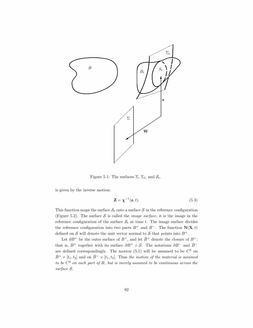
BBt
Σ
Σt
St
W
z
6
+
Figure 5.1: The surfaces Σ, Σt, and St.
is given by the inverse motion:
Z = χ−1(z, t). (5.3)
This function maps the surface St onto a surface S in the reference configuration(Figure 5.2). The surface S is called the image surface; it is the image in thereference configuration of the surface St at time t. The image surface dividesthe reference configuration into two parts B+ and B−. The function N(X, t)defined on S will denote the unit vector normal to S that points into B+.
Let ∂B+ be the outer surface of B+, and let B+ denote the closure of B+;that is, B+ together with its surface ∂B+ + S. The notations ∂B− and B−
are defined correspondingly. The motion (5.1) will be assumed to be C2 onB+ × [t1, t2] and on B− × [t1, t2]. Thus the motion of the material is assumedto be C2 on each part of B, but is merely assumed to be continuous across thesurface S.
92

S St
B−B−
t
B+ B+t
N n
Z z
∂B+
∂B−
6
HHHHHHHHHHHHHHHHY
XXXXz*
Figure 5.2: The surface St and the image surface S.
Consider a field f (X, t), and define f+ by
f+ = limX→Z
f (X, t), (5.4)
where the limit is taken as X approaches Z along a smooth path within B+.The notation f− is defined correspondingly. With some exceptions that will beobvious from their contexts, the superscripts + and − will refer to these limits.The jump of f (X, t) across S is defined by
[[f ]] = f+ − f−. (5.5)
In terms of the mapping (5.2), the velocity of the surface point W is
z =∂
∂tζ(W, t). (5.6)
The normal component z ·n is the speed of the surface St. It is called the speedof displacement ([71], p. 499). From (5.3), the velocity of the surface point W
93

relative to the reference configuration is
Z =∂
∂tχ−1(ζ(W, t), t)
=(∂χ−1
∂x
)+∂ζ
∂t+(∂χ−1
∂t
)+
=(∂χ−1
∂x
)−∂ζ
∂t+(∂χ−1
∂t
)−
.
(5.7)
The chain rules in these expressions can be written in terms of the limits ofthe derivatives at S as a consequence of Hadamard’s lemma ([71], pp. 492-505).Notice that
dX =∂χ−1
∂xdx +
∂χ−1
∂tdt, (5.8)
so the partial derivative of the inverse motion with respect to time holding Xfixed can be written in terms of the inverse of the deformation gradient and thevelocity of the material:
∂χ−1
∂t= −∂χ
−1
∂x
[dxdt
]
X
= −F−1v. (5.9)
Substituting this result into (5.7) yields a relation between the velocity of thematerial point W and the velocity of its image in the reference configuration:
Z = (F−1)+(z− v+)
= (F−1)−(z − v−).(5.10)
The normal component Z · N is the speed of the image surface S relative tothe reference configuration. It is called the speed of propagation ([71], p. 508).Equation (5.10) yields the result
[[F−1(z − v)]] = o. (5.11)
This equation results from the assumed continuity of the motion (5.1) across S.Taking the inner product of (5.11) with N and using (2.66) and (2.71) yieldsthe Stokes-Christoffel condition ([71], p. 522)
[[ρ(z − v) · n]]. (5.12)
This jump condition insures conservation of mass of the material across St.To apply Hamilton’s principle, a comparison motion of the material is defined
by2
x∗ = χ(X, t) + εη(X, t)
= K(X, t, ε).(5.13)
2See the discussion of the comparison motion in Section 2.3.
94

The vector field η(X, t) is arbitrary subject to the conditions that it be C2 onB+ × [t1, t2] and on B− × [t1, t2], that η(X, t1) = o and η(X, t2) = o, and that(5.13) satisfy prescribed boundary conditions on ∂B.3 The field η(X, t) is notassumed to be continuous across S.
A comparison density field is defined by
ρ∗ = ρ(X, t) + εr(X, t), (5.14)
where r(X, t) is an arbitrary scalar field subject to the conditions that it be C1
on B+ × [t1, t2] and on B−× [t1, t2] and that r(X, t1) = 0 and r(X, t2) = 0. Thefield r(X, t) is not assumed to be continuous across S.
In analogy with (5.13), a comparison motion of the surface St is defined by[67]
z∗ = ζ(W, t) + εµ(W, t), (5.15)
where µ(W, t) is an arbitrary C2 function on Σ× [t1, t2] such that µ(W, t1) = oand µ(W, t2) = o.
As a result of the comparison motions (5.13) and (5.15), the position in thereference configuration of the material point that is located at z∗ at time t is(Figure 5.3)
Z∗ = K−1(z∗, t, ε). (5.16)
Expanding this expression with respect to ε yields
Z∗ = Z +
[(∂K−1
∂z∗
)+∂z∗
∂ε+(∂K−1
∂ε
)+]
ε=0
ε+ O(ε2)
= Z + (F−1)+(µ − η+)ε +O(ε2),
(5.17)
where the result (4.18) has been used. This equation also holds when the +superscripts are replaced by −. Introducing the notation (2.88), (5.17) yieldsthe result
δZ = (F−1)+(δz − δx+)
= (F−1)−(δz− δx−),(5.18)
where δz = µ. Therefore,
[[F−1(δz− δx)]] = o. (5.19)
This equation is a constraint imposed on the comparison motions (5.13) and(5.15) by the continuity of the motion of the material at the surface S. CompareEquations (5.18) and (5.19) to Equations (5.10) and (5.11).
3Because the example to be presented is an ideal fluid, and there will be no concern withboundary conditions, it will be assumed henceforth that η · n = 0 on ∂Bt.
95

S
uZ
uZ∗
St
uz
uz∗
Figure 5.3: The points Z∗ and z∗.
Let f (X, t) be a field that is continuous on B+ × [t1, t2] and on B− × [t1, t2],and let f∗(X, t, ε) be its associated comparison field. Consider the integral
I =∫
B±t
ρf dVt =∫
B±ρRf dV , (5.20)
where the notation B±t means the sum of the integrals over B+
t and B−t . The
value of this integral when it is expressed in terms of the comparison fieldf∗(X, t, ε) and the comparison motions (5.13) and (5.15) is (see Figure 5.3)
I∗(ε) =∫
B±ρRf∗ dV −
∫
S[[ρRf [(Z∗ − Z) ·N] ]]dS + O(ε2). (5.21)
The second integral in this expression is due to the displacement of the surface S.Taking the derivative of (5.21) with respect to ε and equating ε to zero, thevariation of the integral is
δI =∫
B±ρR δf dV −
∫
S[[ρRf (δZ ·N)]] dS. (5.22)
By using the results (2.66), (2.71), and (5.18), this variation can be expressedin terms of integrals over Bt and St:
δI =∫
B±t
ρ δf dVt −∫
St
[[ρf (δz− δx) · n]]dSt. (5.23)
96

As an example of the application of these results, consider the kinetic energyof the material contained in Bt
4
T =∫
B±t
12ρv · v dVt =
∫
B±
12ρRv · v dV . (5.24)
The integral of the kinetic energy with respect to time from t1 to t2 is
I =∫ t2
t1
T dt =∫ t2
t1
∫
B±
12ρRv · v dV dt. (5.25)
From (5.22), the variation of this integral is
δI =∫ t2
t1
[∫
B±ρRv · η dV −
∫
S[[12ρR(v · v)(δZ ·N)]]dS
]dt, (5.26)
where η = δx. To integrate the first term in this expression by parts, themotion of the image surface S must be accounted for. This can be done by firstevaluating the derivative
d
dt
∫
B±ρRv · η dV =
∫
B±ρRa · η dV +
∫
B±ρRv · η dV
−∫
S[[ρR(v · η)(Z ·N)]]dS.
(5.27)
Integrating this equation with respect to time from t1 to t2 and noting that ηvanishes at t1 and t2 yields the desired integration by parts:
∫ t2
t1
∫
B±ρRv · η dV dt =
∫ t2
t1
[−∫
B±ρRa · η dV
+∫
S[[ρR(v · η)(Z ·N)]] dS
]dt.
(5.28)
Using this result, the variation of the kinetic energy is
δT = −∫
B±ρRa · δx dV +
∫
S[[(ρRv ⊗ Z)N · δx]] dS
−∫
S[[12ρR(v · v)N · δZ]]dS
= −∫
B±t
ρa · δx dVt +∫
St
[[[ρv⊗ (z− v)]n · δx]]dSt
−∫
St
[[12ρ(v · v)n · (δz − δx)]]dSt,
(5.29)
where the relations (2.71), (5.10), and (5.18) have been used.4See the treatment of this example in Section 2.3.
97

As a second example, consider the constraint term associated with the equa-tion of conservation of mass5
C =∫
B±π
(J − ρR
ρ
)dV =
∫
B±t
π
(1− ρR
ρJ
)dVt. (5.30)
From (5.22), the variation is
δC =∫
B±πJ
(div η +
r
ρ
)dV =
∫
B±t
π
(div η +
r
ρ
)dVt, (5.31)
where r = δρ. To apply the divergence theorem to the first terms in the inte-grands, the presence of the singular surface must be taken into account. Whenthis is done, the variation can be written
δC =∫
B±t
π
(−grad π · δx +
π
ρδρ
)dVt −
∫
St
[[πn · δx]]dSt. (5.32)
The results discussed in this section are quite general and could be appliedto any of the examples in Chapter 3. In the next section their use will beillustrated using the specific case of an elastic ideal fluid.
5.2 An Ideal Fluid Containing a Singular Sur-face
Consider an elastic fluid that occupies a bounded regular region B at time t1.6
Let it be assumed that during the time interval [t1, t2] the volume Bt is dividedinto two parts B+
t and B−t by a singular surface St. Hamilton’s principle states:
Among comparison motions (5.13), comparison density fields (5.14),and comparison motions (5.15) of the singular surface, the actualfields are such that
∫ t2
t1
[δ(T − U ) + δW + δC]dt = 0, (5.33)
where5See the treatment of this example in Section 2.3.6See the discussion of ideal fluids in Section 3.1.1.
98

T =∫
B±t
12ρv · v dVt,
U =∫
B±t
ρe(ρ) dVt,
δW =∫
B±t
ρb · δx dVt,
δC =∫
B±t
(−grad π · δx +
π
ρδρ
)dVt −
∫
St
[[πn · δx]]dSt
+∫
St
ν · [[F−1(δz − δx)]] dSt.
(5.34)
Here the constraint term δC contains both the constraint (5.32) arising fromthe conservation of mass and the constraint (5.19) imposed by the continuityof the motion at St. The vector field ν(z, t) is a Lagrange multiplier that isassumed to be continuous on St × [t1, t2].
By using the result (5.22) and the expression (5.29), (5.33) can be written∫ t2
t1
−∫
B±t
ρa · δx dVt +∫
St
[[[ρv⊗ (z− v)]n · δx]]dSt
−∫
St
[[12ρ(v · v)n · (δz − δx)]] dSt
−∫
B±t
ρde
dρδρ dVt +
∫
St
[[ρe(δz− δx) · n]]dSt
+∫
B±t
ρb · δx dVt +∫
B±t
(−grad π · δx +
π
ρδρ
)dVt
−∫
St
[[πn · δx]]dSt +∫
St
ν · [[F−1(δz − δx)]] dSt
dt = 0.
(5.35)
If it is assumed that δz = o and that the variations δx± vanish on St, (5.35)reduces to the case considered in Section 3.1.1 and yields the equation of balanceof linear momentum (3.18) on B+×[t1, t2] and on B−×[t1, t2]. As a consequence,only the terms involving integrals over St remain in (5.35). Next, let δx± = oin (5.35) while δz is permitted to be arbitrary on St. This results in the jumpcondition
[[−12ρ(v · v)n + ρen + F−1ν]] = o on St × [t1, t2] . (5.36)
Finally, permitting the variations δx+ and δx− to be arbitrary in (5.35) yieldsthe two equations
[ρv ⊗ (z− v)]n + 12ρ(v · v)n− ρen− πn−F−tν± = o. (5.37)
99

Subtracting the − equation from the + equation and adding the result to (5.36)results in the jump condition
[[[ρv⊗ (z − v)]n− πn]] = o on St × [t1, t2] . (5.38)
This is the momentum jump condition. It insures conservation of linear momen-tum of the material across St (see e.g. [27], pp. 104-106).
Eliminating the Lagrange multiplier ν from the two equations (5.37) resultsin the jump condition
[[Ft[ρv ⊗ (z − v)]n + 12ρ(v · v)n− ρen − πn]] = o on St × [t1, t2] . (5.39)
Taking the inner product of this equation with Z, taking the inner product of(5.38) with z, and summing the results leads with some rearrangement to theusual form of the energy jump condition
[[ρ(e+ 12v · v)[(z− v) · n]− π(v · n)]] = 0 on St × [t1, t2] . (5.40)
This equation insures conservation of energy of the material across St (see e.g.[27], pp. 121-123). This derivation of the energy jump condition did not includeterms associated with heat conduction.
Thus Hamilton’s principle yields both the linear momentum and the energyjump conditions for the fluid. This procedure has been extended to mixtures offluids and elastic materials by Batra [3] and Batra, et al. [4]. It could potentiallybe extended to other generalized theories of continuous media.
100

Acknowledgments
This monograph is a result of my fifteen year professional collaboration withDouglas Drumheller of Sandia National Laboratories. Our work on mixturesled us to become interested in Hamilton’s principle, and in addition to his orig-inal contributions to the research, Doug helped me understand many of thesubtleties of variational methods in continuum mechanics. Chapter 4 is basedin large part on our results. Our collaboration took place during periods whenI was a temporary staff member and consultant at Sandia. I am grateful forthe courteous and generous treatment I received from that organization, andparticularly want to thank Jim Asay, Darrel Munson, and Walt Hermann. Ithank the United States Department of Energy for their support of my workthere. Much of the work on which Chapter 5 is based was done in collaborationwith Gautam Batra, and the monograph also benefited from his ideas on nota-tion and the organization of the subject. Part of the manuscript was writtenwhile I was a member of the technical staff at Applied Research Laboratories,University of Texas at Austin. I thank the Office of Naval Research for theirsupport of my work there. Gautam Batra, Ray Bowen, Doug Drumheller, MortGurtin, Steve Passman, Morris Stern, and Tim Trucano read an early draft andgave me many helpful suggestions.
101

Bibliography
[1] Akhiezer, N. I., The Calculus of Variations, CRC Press, Boca Raton,Florida, 1988.
[2] Bateman, H., “Hamilton’s work in dynamics and its influence on modernthought,” A Collection of Papers in Memory of Sir William Rowan Hamil-ton, pp. 51-64, Kessinger Publishing LLC, Whitefish, Montana, 2010.
[3] Batra, G., On the Propagation of One-Dimensional Waves of Discontinuityin Mixtures, Ph.D. Dissertation, The University of Texas at Austin, Austin,Texas, 1984.
[4] Batra, G., Bedford, A., and Drumheller, D. S., “Applications of Hamil-ton’s principle to continua with singular surfaces,” Archive for RationalMechanics and Analysis 93, 223-251, 1986.
[5] Bedford, A., and Drumheller, D. S., “A variational theory of immisciblemixtures,” Archive for Rational Mechanics and Analysis 68, 37-51, 1978.
[6] Bedford, A., and Drumheller, D. S., “A variational theory of porous media,”International Journal of Solids and Structures 15, 967-980, 1979.
[7] Bedford, A., and Drumheller, D. S., “Theories of Immiscible and StructuredMixtures,” International Journal of Engineering Science 21, 863-960, 1983.
[8] Bedford, A., and Stern, M., “A model for wave propagation in gassy sedi-ments,” Journal of the Acoustical Society of America 73, 409-417, 1983.
[9] Berryman, J. G., and Thigpen, L., “Nonlinear and semilinear dynamicporoelasticity with microstructure,” Journal of the Mechanics and Physicsof Solids 33, 97-116, 1985.
[10] Biot, M. A., “Theory of propagation of elastic waves in a fluid-saturatedporous solid—I. Low frequency range,” Journal of the Acoustical Society ofAmerica 28, 168-178, 1956.
102

[11] Bliss, G. A., Lectures on the Calculus of Variations, University of ChicagoPress, Chicago, Illinois, 1961.
[12] Bolza, O., Lectures on the Calculus of Variations, Chelsea Publishing Com-pany, New York, 1960.
[13] Bowen, R. M., “Theory of Mixtures,” Continuum Physics Vol. III, Mixturesand EM Field Theories, pp. 1-127, edited by A. C. Eringen, AcademicPress, New York, 1976.
[14] Bowen, R. M., and Wang, C. -C., Intoduction to Vectors and Tensors,Dover Publications, Mineola, New York, 2009.
[15] Courant, R., and Hilbert, D., Methods of Mathematical Physics Vol. I,Wiley, New York, 1989.
[16] Cowin, S. C., “A theory for the flow of granular materials,” Powder Tech-nology 9, 61-69, 1974.
[17] Cowin, S. C., and Goodman, M. A. “A variational principle for granularmaterials,” ZAMM 56, 281-286, 1976.
[18] Cowin, S. C., and Nunziato, J. W. “Waves of dilantancy in a granularmaterial with incompressible grains,” International Journal of EngineeringScience 19, 993-1008, 1981.
[19] Craine, R. E., “Oscillations of a plate in a binary mixture of incompressibleNewtonian fluids,” International Journal of Engineering Science 9, 1177-1192, 1971.
[20] Drew, D. A., “Two-phase flows: Constitutive equations for lift and Brow-nian motion and some basic flows,” Archive for Rational Mechanics andAnalysis 62, 149-163, 1976.
[21] Drumheller, D. S., and Bedford, A.,“A theory of bubbly liquids,” Journalof the Acoustical Society of America 66, 197-208, 1979.
[22] Drumheller, D. S., and Bedford, A.,“A thermomechanical theory for re-acting immiscible mixtures,” Archive for Rational Mechanics and Analysis73, 257-284, 1980.
[23] Drumheller, D. S., Kipp, M. E., and Bedford, A.,“Transient wave propaga-tion in bubbly liquids,” Journal of Fluid Mechanics 119, 347-365, 1982.
103
[24] Eckart, C.,“Variational principles of hydrodynamics,” Physics of Fluids 3,421-427, 1960.
[25] Ericksen, J. L.,“Tensor fields,” Encyclopedia of Physics Vol. III/1, editedby S. Flugge, pp. 794-858, Springer-Verlag, Berlin-Gottingen-Heidelberg,1960.
[26] Ericksen, J. L.,“Conservation laws for liquid crystals,” Transactions of theSociety of Rheology 5, 23-34, 1961.
[27] Eringen, A. C., Mechanics of Continua, Robert E. Krieger Publishing Co.,Huntington, New York, 1980.
[28] Finlayson, B. A., The Method of Weighted Residuals and Variational Prin-ciples, Society for Industrial and Applied Mathematics, Philadelphia, 2014.
[29] Gelfand, I. M., and Fomin, S. V., Calculus of Variations, Dover Publica-tions Mineola, New York, 2000.
[30] Goldstein, H., Poole, C. P., and Safko, J., Classical Mechanics, PearsonEducation, Upper Saddle River, New Jersey, 2011.
[31] Goodman, M. A., and Cowin, S. C.,“A continuum theory for granularmaterials,” Archive for Rational Mechanics and Analysis 44, 249-266, 1972.
[32] Graves, R. P., Life of Sir William Rowan Hamilton, Ulan Press, 2012.
[33] Gurtin, M. E., “Variational Principles for Linear Elastodynamics,” Archivefor Rational Mechanics and Analysis 16, 34-50, 1964.
[34] Gurtin, M. E.,“The linear theory of elasticity,” Encyclopedia of PhysicsVol. VIa/2, edited by C. Truesdell, pp. 1-295, Springer-Verlag, Berlin-Gottingen-Heidelberg, 1972.
[35] Gurtin, M. E., An Introduction to Continuum Mechanics, Academic Press,New York, 1981.
[36] Halmos, P. R., Finite-Dimensional Vector Spaces, Martino Fine Books,Eastford, Connecticut, 2012.
[37] Hamilton, W. R., “Theory of systems of rays,” Transactions of the RoyalIrish Academy 15, 69-174, 1828.
[38] Hamilton, W. R., “On a general method in dynamics,” Philosophical Trans-actions of the Royal Society of London, Part II, 247-308, 1834.
104

[39] Hamilton, W. R., “Second essay on a general method in dynamics,” Philo-sophical Transactions of the Royal Society of London, Part I, 95-144, 1835.
[40] Hamilton, W. R., The Mathematical Papers of Sir William Rowan Hamil-ton, Vol. I, Geometrical Optics, edited by A. W. Conway and J. L. Synge,Cambridge University Press, London, 1931.
[41] Hamilton, W. R., The Mathematical Papers of Sir William Rowan Hamil-ton, Vol. II, Dynamics, edited by A. W. Conway and A. J. McConnell,Cambridge University Press, London, 1940.
[42] Hankins, T. L., Sir William Rowan Hamilton, Johns Hopkins UniversityPress, Baltimore, Maryland, 1980.
[43] Herivel, J. W., “The derivation of the equations of motion of an idealfluid by Hamilton’s principle,” Proceedings of the Cambridge PhilosophicalSociety 51, 344-349, 1955.
[44] Hill, C. D., “Two-dimensional analysis of the stability of particulate sedi-mentation,” Physics of Fluids 23, 667-668, 1980.
[45] Hill, C. D., and Bedford, A., “Stability of the equations for particulatesedimentation,” Physics of Fluids 22, 1252-1254, 1979.
[46] Hill, C. D., and Bedford, A., “A model for erythrocyte sedimentation,”Biorheology 18, 255-266, 1981.
[47] Hill, C. D., Bedford, A., and Drumheller, D. S., “An application of mixturetheory to particulate sedimentation,” Journal of Applied Mechanics 47,261-265, 1980.
[48] Knowles, J. K., Linear Vector Spaces and Cartesian Tensors, Oxford Uni-versity Press, New York, 1997.
[49] Kuznetsov, V. V., Nakoryakov, V. E., Pokusaev, B. G., and Shreiber, I.R.,“Propagation of perturbations in a gas-liquid mixture,” Journal of FluidMechanics 85, 85-96, 1978.
[50] Lanczos, C., The Variational Principles of Mechanics, Dover Publications,Mineola, New York, 1986.
[51] Leech, C. M.,“Hamilton’s principle applied to fluid mechanics,” QuarterlyJournal of Mechanics and Applied Mathematics 30, 107-130, 1977.
105

[52] Leigh, D. C., Nonlinear Continuum Mechanics, McGraw-Hill, New York,1968.
[53] Love, A. E. H., A Treatise on the Mathematical Theory of Elasticity, Cam-bridge University Press, London, 2013.
[54] Mindlin, R. D., “Micro-structure in linear elasticity,” Archive for RationalMechanics and Analysis 16, 51-78, 1964.
[55] Nowinski, J. L., Theory of Thermoelasticity with Applications, Springer,Berlin, 2011.
[56] Nunziato, J. W., and Passman, S. L.,“A multiphase mixture theory forfluid-saturated granular materials,” Mechanics of Structured Media A,edited by A. P. S. Selvadurai, pp. 243-254, Elsevier, Amsterdam, 1981.
[57] Nunziato, J. W., Passman, S. L., and Thomas, J. P. “Gravitational flowof granular materials with incompressible grains,” Journal of Rheology 24,395-420, 1980.
[58] Nunziato, J. W., and Walsh, E. K., “One-dimensional shock waves in uni-formly distributed granular materials,” International Journal of Solids andStructures 14, 681-689, 1978.
[59] Nunziato, J. W., and Walsh, E. K., “On ideal multiphase mixtures withchemical reactions and diffusion,” Archive for Rational Mechanics andAnalysis 73, 285-311, 1980.
[60] Oden, J. T., and Reddy, J. N., Variational Methods in Theoretical Mechan-ics, Springer-Verlag, Berlin-Gottingen-Heidelberg, 1976.
[61] Pars, L. A., An Introduction to the Calculus of Variations, Dover Publica-tions, Mineola, New York, 2009.
[62] Passman, S. L. “Mixtures of granular materials,” International Journal ofEngineering Science 15, 117-129, 1977.
[63] Passman, S. L. “Shearing flows of granular materials,” Journal of the En-gineering Mechanics Division of the American Society of Civil Engineers106, 773-783, 1980.
[64] Passman, S. L., Nunziato, J. W., and Walsh, E. K., “A theory of multiphasemixtures,” appendix to Rational Thermodynamics by C. Truesdell, pp. 286-325, Springer-Verlag, New York-Berlin-Heidelberg-Tokyo, 1984.
106

[65] Serrin, J.,“Mathematical principles of classical fluid mechanics,” Encyclo-pedia of Physics Vol. VIII/1, edited by S. Flugge and C. Truesdell, pp.125-263, Springer-Verlag, Berlin-Gottingen-Heidelberg, 1959.
[66] Silberman, E.,“Sound velocity and attenuation in bubbly mixtures mea-sured in standing wave tubes,” Journal of the Acoustical Society of America29, 925-933, 1957.
[67] Taub, A. H.,“On Hamilton’s principle for perfect compressible fluids,”Nonlinear Problems in Mechanics of Continua, edited by E. Reissner,W. Prager, and J. J. Stoker, American Mathematical Society, New York,1949.
[68] Torby, B. J., Advanced Dynamics for Engineers, Holt, Rinehart and Win-ston, New York, 1984.
[69] Truesdell, C., and Wang, C. -C., Rational Thermodynamics, Springer-Verlag, New York-Berlin-Heidelberg-Tokyo, 2011.
[70] Truesdell, C., and Noll, W.,“The non-linear field theories of mechanics,”Encyclopedia of Physics Vol. III/3, edited by S. Flugge, Springer-Verlag,Berlin-Heidelberg-New York, 1965.
[71] Truesdell, C., and Toupin, R. A.,“The classical field theories,” Encyclo-pedia of Physics Vol. III/1, edited by S. Flugge, Springer-Verlag, Berlin-Gottingen-Heidelberg, 1960.
[72] van Wijngaarden, L.,“One-dimensional flow of liquids containing small gasbubbles,” Annual Reviews of Fluid Mechanics 4, 369-396, 1972.
[73] Washizu, K., Variational Methods in Elasticity and Plasticity, PergamonPress, New York, 1982.
[74] Weinstock, R., Calculus of Variations, Nabu Press, Charleston, South Car-olina, 2014.
[75] Whelan, J. A., Huang, C. -R., and Copley, A. L.,“Concentration profiles inerythrocyte sedimentation in human whole blood,” Biorheology 7, 205-212,1971.
[76] Whittaker, E. T., A Treatise on the Analytical Dynamics of Particles andRigid Bodies, Cambridge University Press, London, 1989.
107
Related Documents