Fisheries Research 73 (2005) 37–47 Incorporating spatial analysis of habitat into spiny lobster (Panulirus argus) stock assessment at Alacranes reef, Yucatan, M´ exico P. Javier Bello a , L. Veronica Rios b,c,∗ , C.M.A. Liceaga c , M. Carlos Zetina d , C. Kenneth Cervera b , B. Patricia Arceo b , N. Hector Hernandez c a Watershed Ecosystems Graduate Program, Trent University, Peterborough, Ont. , Canada K9J 7B8 b Centro de Investigaci´ on Pesquera Yucalpet´ en, Instituto Nacional de la Pesca, A.P. 73 Progreso, Yucatan, M´ exico c Centro de Investigaci´ on y Estudios Avanzados-Merida, A.P. 73 Cordemex, Merida, Yucatan, M´ exico d Facultad de Ingenier´ ıa Universidad Autonoma de Yucatan, A.P. 150 Cordemex, Merida, Yucatan, M´ exico Received 8 July 2003; received in revised form 24 September 2004; accepted 11 January 2005 Abstract In this paper, spatial analysis of submerged habitats was incorporated into spiny lobster (Panulirus argus) stock assessment at Alacranes reef, Yucatan, M´ exico. Two sources of information were used: a thematic map of submerged habitats obtained using a Landsat TM satellite image and “geo-referenced” field data for lobster catches obtained during July 1998 and February 1999. Geographical information systems (GIS) tools were used as the major basis for displaying, analysing and relating lobster catches data and the thematic map information. Estimations of lobster abundance, density and biomass per habitat class and for the whole reef, at the beginning and end of the fishing season, were obtained. Utilizing Monte Carlo modelling, uncertainty was incorporated to estimations of transects initial and final position, appreciation of area and probability to detect lobsters. Results were compared against commercial catches reported for the previous year. The distribution of fishing effort is also described. © 2005 Elsevier B.V. All rights reserved. Keywords: Landsat TM; GIS; Panulirus argus; Habitat mapping; Stock assessment; Lobster fishery ∗ Corresponding author. Tel.: +52 969 9 35 40 28; fax: +52 969 9 35 40 28. E-mail addresses: [email protected] (P.J. Bello), g [email protected] (L.V. Rios). 1. Introduction To increase the protection of its resources, the Alacranes reef was declared a National Park in 1994 (Ardisson et al., 1996), nevertheless, the reef has a traditional importance for fisheries of species with high 0165-7836/$ – see front matter © 2005 Elsevier B.V. All rights reserved. doi:10.1016/j.fishres.2005.01.013

Welcome message from author
This document is posted to help you gain knowledge. Please leave a comment to let me know what you think about it! Share it to your friends and learn new things together.
Transcript
Fisheries Research 73 (2005) 37–47
Incorporating spatial analysis of habitat into spiny lobster(Panulirus argus) stock assessment at Alacranes reef,
Yucatan, Mexico
P. Javier Belloa, L. Veronica Riosb,c,∗, C.M.A. Liceagac,M. Carlos Zetinad, C. Kenneth Cerverab, B. Patricia Arceob,
N. Hector Hernandezc
a Watershed Ecosystems Graduate Program, Trent University, Peterborough, Ont. , Canada K9J 7B8b Centro de Investigaci´on Pesquera Yucalpet´en, Instituto Nacional de la Pesca, A.P. 73 Progreso, Yucatan, M´exico
c Centro de Investigaci´on y Estudios Avanzados-Merida, A.P. 73 Cordemex, Merida, Yucatan, M´exicod Facultad de Ingenier´ıa Universidad Autonoma de Yucatan, A.P. 150 Cordemex, Merida, Yucatan, M´exico
Received 8 July 2003; received in revised form 24 September 2004; accepted 11 January 2005
Abstract
In this paper, spatial analysis of submerged habitats was incorporated into spiny lobster (Panulirus argus) stock assessmentat Alacranes reef, Yucatan, Mexico. Two sources of information were used: a thematic map of submerged habitats obtained
ebruaryg lobsterclass and
ertaintyobsters.t is also
he94ah
using a Landsat TM satellite image and “geo-referenced” field data for lobster catches obtained during July 1998 and F1999. Geographical information systems (GIS) tools were used as the major basis for displaying, analysing and relatincatches data and the thematic map information. Estimations of lobster abundance, density and biomass per habitatfor the whole reef, at the beginning and end of the fishing season, were obtained. Utilizing Monte Carlo modelling, uncwas incorporated to estimations of transects initial and final position, appreciation of area and probability to detect lResults were compared against commercial catches reported for the previous year. The distribution of fishing effordescribed.© 2005 Elsevier B.V. All rights reserved.
Keywords:Landsat TM; GIS;Panulirus argus; Habitat mapping; Stock assessment; Lobster fishery
∗ Corresponding author. Tel.: +52 969 9 35 40 28;fax: +52 969 9 35 40 28.
E-mail addresses:[email protected] (P.J. Bello),g [email protected] (L.V. Rios).
1. Introduction
To increase the protection of its resources, tAlacranes reef was declared a National Park in 19(Ardisson et al., 1996), nevertheless, the reef hastraditional importance for fisheries of species with hig
0165-7836/$ – see front matter © 2005 Elsevier B.V. All rights reserved.doi:10.1016/j.fishres.2005.01.013
38 P.J. Bello et al. / Fisheries Research 73 (2005) 37–47
commercial value such as lobsters, groupers and snap-pers (Rıos et al., 1998a). More than 15% of the spinylobster (Panulirus argus) total catches for the state ofYucatan are from this area and surroundings (Rıos etal., 1998a). The lobster-fishing season extends fromJuly to February. Four fishermen unions operate in thearea, using a total of 12 vessels, 35–55 ft long. Eachship is used as a tender for five to seven small boatscalled “alijos”. Some alijos are 10 ft long without mo-tor and some are about 16 ft long with 10 HP outboards.Depending on depth, fishermen use snorkel divingor air pumped from a compressor called a “hookah”to search for lobsters. They use a hook called a“bichero”, as the direct catching instrument (Rıos et al.,1998a).
The distribution of fishing effort over the reef has aregular seasonal pattern. At the beginning of the sea-son, fishers go to the central reef flat, where shallowcoral patches are common, an area well known to pro-vide shelter for lobsters. In the last few months of theseason, and once the central area has been harvested,crafts move toward northwest and southeast deeper ar-eas of the reef, where it is more difficult to catch lobsterbecause probable shelters are dispersed, and at greaterdepth (Rıos et al., 1998a).
To achieve the sustainable use and development ofcoral reef resources, it is necessary to incorporate effec-tive planning and management strategies. Such strate-gies should allow for the incorporation of the views,opinions and knowledge of the key stakeholders, alongw theg andm
thel entrei esti-m as-s ents -f inedf ro-g ea re-s
y in-c tiono s,1 nd
extensive studies implying a large sampling effort arerequired (Evans and Evans, 1996).
In recent years, remote sensing technology and geo-graphical information systems (GIS) have proven to bepowerful tools for to the evaluation of coastal and ma-rine habitats (Green et al., 2000) and particularly to cal-culate the extension of preferential habitat for speciesof commercial value (Jones and Stoner, 1997; Green etal., 1996).
Preferential habitats for different stages of lob-ster development have been well documented for theCaribbean area (Davidson et al., 2002; Childress andHerrnkind, 1996; Herrera and Ibarzabal, 1995). Spinylobster uses cryptic habitats (Davidson et al., 2002),showing preference for particular areas where they canfind shelter and food.
In the case of Alacranes reef,Liceaga et al. (1997),made a first attempt to define lobster distribution areasby displaying lobster abundances field data on “unsu-pervised” classified satellite images. They estimatedhigher densities for those classes located toward thecentre of the reef, but they were not able to relate suchinformation with particular habitats.
In this study, we discuss the potential of satelliteimagery analyses and GIS tools for incorporating spa-tial analysis of submerged habitats for the estimationof spiny lobster (P. argus) abundance, density andbiomass at the Alacranes reef, for both the beginningand at the end of the fishing season.
2
2
kmn Yu-c heraI ri-e idtha adeu itsm reefs thel andyi
ith the technical and scientific propositions byroups of scientists, and those of the local usersanagers (Crosby et al., 2002).To provide decision-makers with information on
obster fishery, the Fisheries Research Regional Cn Yucatan has conducted a series of surveys for
ating spiny lobster densities to be used in stockessment and for modelling the population replacemtatus (Rıos et al., 1998b). Until recently, the only inormation available for those estimations was obtarom records of lobster “tails” landed at Puerto Preso, Yucatan (Rıos et al., 1998b), making impossiblny consideration on the spatial distribution of theource at the reef.
Lobster stock assessment can be improved borporating spatial analysis of habitat and informan their likely area of distribution (Evans and Evan996). However, this is very difficult to estimate, a
. Methods
.1. Study area
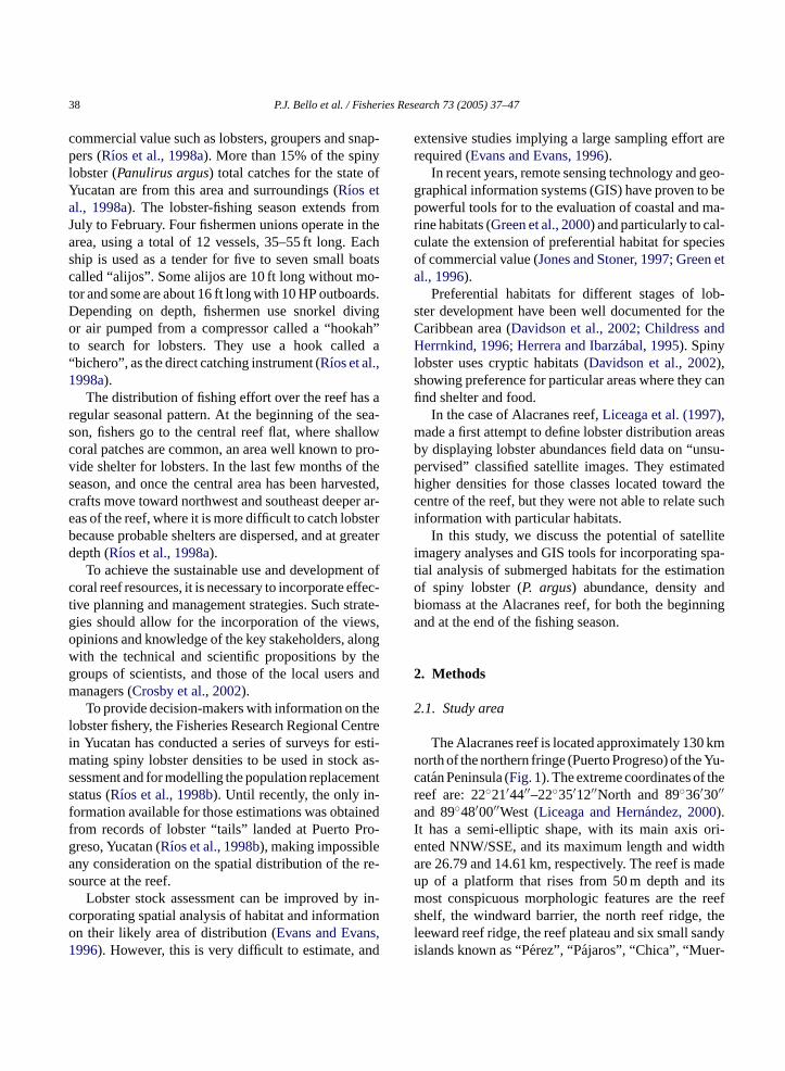
The Alacranes reef is located approximately 130orth of the northern fringe (Puerto Progreso) of theatan Peninsula (Fig. 1). The extreme coordinates of teef are: 22◦21′44′′–22◦35′12′′North and 89◦36′30′′nd 89◦48′00′′West (Liceaga and Hernandez, 2000).
t has a semi-elliptic shape, with its main axis onted NNW/SSE, and its maximum length and wre 26.79 and 14.61 km, respectively. The reef is mp of a platform that rises from 50 m depth andost conspicuous morphologic features are the
helf, the windward barrier, the north reef ridge,eeward reef ridge, the reef plateau and six small sslands known as “Perez”, “Pajaros”, “Chica”, “Muer-
P.J. Bello et al. / Fisheries Research 73 (2005) 37–47 39
Fig. 1. Geographic location of Alacranes reef.
tos”, “Desterrada” and “Desaparecida” (Bonet, 1967;De la Cruz et al., 1993; Ardisson et al., 1996).
2.2. Elaboration of a submerged habitats map
The map of submerged habitats used in this studywas developed from the analysis of a multi-spectralLandsat TM image and field data.
2.2.1. Landsat TM image preprocessingFrom a Landsat TM image obtained in February
1998, a work sub-image (1000 pixels× 1000 pixels)was extracted. Bands 1, 2, 3 and 7 of this sub-imagewere geo-referenced using a first order polynomialtransformation and 10 ground control points verifiedin the field with a global position system (GPS), ob-taining a mean RMS error value of 5.2 m.
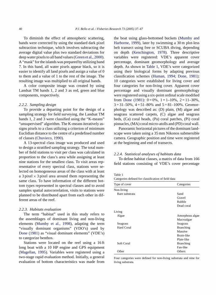
40 P.J. Bello et al. / Fisheries Research 73 (2005) 37–47
To diminish the effect of atmospheric scattering,bands were corrected by using the standard dark pixelsubtraction technique, which involves subtracting theaverage digital value plus two standard deviations fordeep water pixels to all band values (Green et al., 2000).A “mask” for the islands was prepared by utilizing band7. In this band, all water pixels appear black, so it iseasier to identify all land pixels and assign a value of 0to them and a value of 1 to the rest of the image. Theresulting image was multiplied to all original bands.
A color composite image was created by usingLandsat TM bands 1, 2 and 3 as red, green and bluecomponents, respectively.
2.2.2. Sampling designTo provide a departing point for the design of a
sampling strategy for field surveying, the Landsat TMbands 1, 2 and 3 were classified using the “K-means”“unsupervised” algorithm. The K-means iteratively as-signs pixels to a class utilizing a criterion of minimumEuclidian distance to the centre of a predefined numberof classes (Chuvieco, 1990).
A 13-spectral class image was produced and usedto design a stratified sampling strategy. The total num-ber of field stations to visit per class was calculated inproportion to the class’s area while assigning at leastnine stations for the smallest class. To visit areas rep-resentative of every spectral class, stations were se-lected on homogeneous areas of the class with at leasta 3 pixel× 3 pixel area around them representing thes bot-t avoids erep dif-f
2to
t inge“ byD s)t
6 ftl ent( at erale rom
the boat using glass-bottomed buckets (Mumby andHarborne, 1999), later by swimming a 30 m plot-lessbelt transect using free or SCUBA diving, dependingon depth (Kenchington, 1978). Three descriptivevariables were registered: VDE’s apparent coverpercentage, dominant geomorphology and averagedepth. As shown inTable 1, VDE’s were categorizedusing their biological forms by adapting previousclassification schemes (Human, 1994; Done, 1981);10 categories were established for living cover andfour categories for non-living cover. Apparent coverpercentage and visually dominant geomorphologywere registered using a six-point ordinal scale modifiedfrom Done (1981): 0 = 0%, 1 = 1–10%, 2 = 11–30%,3 = 31–50%, 4 = 51–80% and 5 = 81–100%. Geomor-phology was described as: (D) plain, (M) algae andseagrass scattered carpets, (C) algae and seagrassbeds, (Ca) coral heads, (Pa) coral patches, (Pi) coralpinnacles, (MA) coral micro-atolls and (PD) coral wall.
Panoramic horizontal pictures of the dominant land-scape were taken using a 35 mm Nikonos submersiblecamera. Geographic position and time were registeredat the beginning and end of transects.
2.2.4. Statistical analyses of habitats dataTo define habitat classes, a matrix of data from 166
field stations consisting of VDE’s cover percentage
Table 1C
T
N
Le
F e forl
ame class. To have information of the differentom types represented in spectral classes and toamples spatial autocorrelation, visits to stations wlanned to be distributed apart from each other in
erent areas of the reef.
.2.3. Habitats evaluationThe term “habitat” used in this study refers
he assemblages of dominant living and non-livlements (Mumby et al., 1998), adapting the termvisually dominant organisms” (VDO’s) usedone (1981)as “visual dominant elements” (VDE’
o categorize benthos.Stations were located on the reef using a 1
ong boat with a 10 HP engine and GPS equipmMagellan, 1995). Variables were registered usingwo-stage rapid evaluation method. Initially, a genvaluation of bottom characteristics was made f
ategories defined for classification of field data
ype of cover Categories
on-livingBare substrata Sand
GravelRubbleDead coral
ivingAlgae Amorphous alga
MacroalgaeSeagrass SeagrassHard Coral Branching
MassiveBrain-likePlate-like
Soft Coral BranchingFan-like
Other Others
our categories were defined for non-living substrata and niniving substrata.
P.J. Bello et al. / Fisheries Research 73 (2005) 37–47 41
and geomorphology was classified using a hierarchicalcluster analysis, including the Gower similarityindex and the unweighed pair group average (UP-GMA) grouping method (Digby and Kempton, 1987;Legendre and Legendre, 1983). Data were alsoanalysed using the canonical correspondence analysis(CCA) ordination method, utilizing geomorphologyand depth as the ordination variables (ter Braakand Verdonschot, 1995). Stations were assigned to25-habitat classes based on the results of both analysesand considered as the ground truth.
2.2.5. Supervised classification of imageStations were labelled in agreement with their field
class and used to generate 25 “training areas” for theclassification of the Landsat image. Training areas aresets of pixels that exemplify each cover type and areused to “train” the software to recognize and to assignall pixels in an image to their appropriate class. Everytraining area consisted of the pixel corresponding tothe field station coordinates and the 3× 3 neighbourpixels.
We used a standard supervised classification ap-proach to produce a preliminary thematic map of sub-merged habitats for the reef. It consisted in utilizingthe maximum likelihood supervised classification algo-rithm (Microimages, 2001) and the training areas pre-viously defined, to classify the Landsat TM bands 1, 2and 3 (Chuvieco, 1990). It resulted in a 25-class image,which appeared highly heterogeneous. By overlayinga ge,w pedw con-f o,1 hei the“ acyo be-t racyo thatc d si-m theh intob assesa ined.T ents:g acyo e of
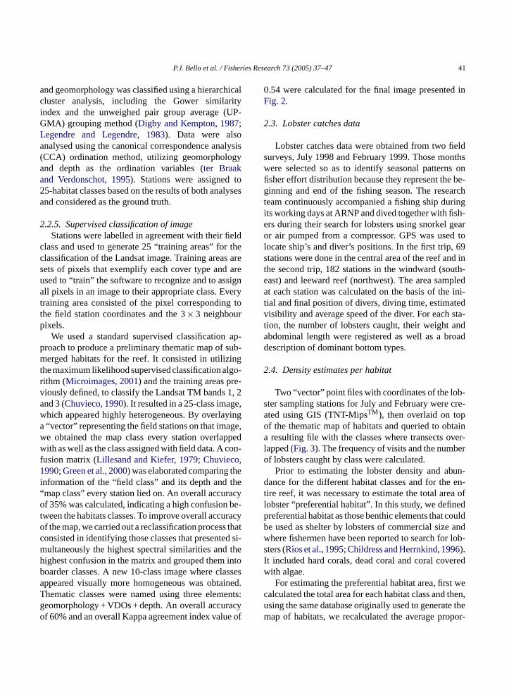
0.54 were calculated for the final image presented inFig. 2.
2.3. Lobster catches data
Lobster catches data were obtained from two fieldsurveys, July 1998 and February 1999. Those monthswere selected so as to identify seasonal patterns onfisher effort distribution because they represent the be-ginning and end of the fishing season. The researchteam continuously accompanied a fishing ship duringits working days at ARNP and dived together with fish-ers during their search for lobsters using snorkel gearor air pumped from a compressor. GPS was used tolocate ship’s and diver’s positions. In the first trip, 69stations were done in the central area of the reef and inthe second trip, 182 stations in the windward (south-east) and leeward reef (northwest). The area sampledat each station was calculated on the basis of the ini-tial and final position of divers, diving time, estimatedvisibility and average speed of the diver. For each sta-tion, the number of lobsters caught, their weight andabdominal length were registered as well as a broaddescription of dominant bottom types.
2.4. Density estimates per habitat
Two “vector” point files with coordinates of the lob-ster sampling stations for July and February were cre-ated using GIS (TNT-MipsTM), then overlaid on topo taina ver-l ero
un-d en-t a ofl edp ouldb andw r lob-s 96I eredw
t wec then,u te them por-
“vector” representing the field stations on that imae obtained the map class every station overlapith as well as the class assigned with field data. A
usion matrix (Lillesand and Kiefer, 1979; Chuviec990; Green et al., 2000) was elaborated comparing t
nformation of the “field class” and its depth andmap class” every station lied on. An overall accurf 35% was calculated, indicating a high confusion
ween the habitats classes. To improve overall accuf the map, we carried out a reclassification processonsisted in identifying those classes that presenteultaneously the highest spectral similarities andighest confusion in the matrix and grouped themoarder classes. A new 10-class image where clppeared visually more homogeneous was obtahematic classes were named using three elemeomorphology + VDOs + depth. An overall accurf 60% and an overall Kappa agreement index valu
f the thematic map of habitats and queried to obresulting file with the classes where transects o
apped (Fig. 3). The frequency of visits and the numbf lobsters caught by class were calculated.
Prior to estimating the lobster density and abance for the different habitat classes and for the
ire reef, it was necessary to estimate the total areobster “preferential habitat”. In this study, we definreferential habitat as those benthic elements that ce used as shelter by lobsters of commercial sizehere fishermen have been reported to search foters (Rıos et al., 1995; Childress and Herrnkind, 19).t included hard corals, dead coral and coral covith algae.For estimating the preferential habitat area, firs
alculated the total area for each habitat class andsing the same database originally used to generaap of habitats, we recalculated the average pro
42 P.J. Bello et al. / Fisheries Research 73 (2005) 37–47
Fig. 2. Thematic map of Alacranes reef submerged habitats.
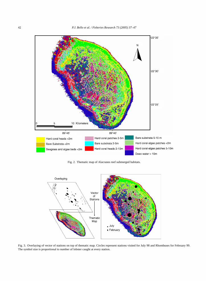
Fig. 3. Overlaying of vector of stations on top of thematic map. Circles represent stations visited for July 98 and Rhombuses for February 99.The symbol size is proportional to number of lobster caught at every station.
P.J. Bello et al. / Fisheries Research 73 (2005) 37–47 43
tion of every class area corresponding to the benthicelements described earlier.
For the estimations of lobster density and abundancewe used an estimator previously tested and reported byRıos et al. (2003), to be appropriate when consideringareas of different size.
The density was calculated using Eq.(1):
R =∑
yi∑zi
(1)
whereR is the estimated mean density,yi the numberof organisms observed andzi is the surveyed area. Thatarea correspond towi × Li × pi. Wherewi is the widthof the transect,Li the length of the transect andpi is theprobability of detecting organisms.
To estimate the total number of organisms in thearea of interest, we used Eq.(2):
ˆY = ˆR × Z (2)
where ˆY is the total number of organisms,ˆR the meandensity of organisms andZ is the area of interest.
Biomass estimates in the area of interest were cal-culated by multiplying the total number of organismsestimated in that area by their average weight for everyfishing trip: July (0.194 kg) and February (0.162 kg),as in Eq.(3):
B = ˆY × mean weight (3)
atedu
V
a ismsi ;S
V
U in-c hicalp ba-b
an-s -i o.).
We used Eq.(6) to estimate length of transect:
Li = Lo + Ep (6)
whereLi is the length of transect,Lo is the length esti-mated using the GPS andEp is the range of error from0 to 50 m for the position of the beginning and end ofthe transects, considering a uniform distribution.
For the estimation of transept width we assignedan appreciation error of 20%, according to empiricalknowledge. We used the following equation:
Wi = wo + Ea (7)
whereWi is transect width,wo is width of transect asappreciated by diver andEa corresponds to the 20%appreciation error, considering a normal distribution.
We assigned different intervals for the probabilityto detect organisms at the beginning and end of season.For July, when there is major abundance of lobsters,we considered an interval of 80–99% and for Febru-ary, when abundance has diminished due to the fishingimpact and it is more difficult to find refugees with lob-sters (Rıos et al., 2003), we considered an interval of30–70%.
Monte Carlo simulation was implemented us-ing Visual-Basic for EXCEL. The model was run10,000 times to calculate the mean density, abundance,biomass and their variances per habitat class and forthe entire reef.
3
ont andt sym-b ghti inge hesf t oft tedh hiled itats.W abi-t y ofv at attm bster
The variance of the mean density was calculsing Eq.(4):
ˆ ( ˆR) =∑
yi∑zi
2
(1 − p
p2
)(4)
nd the variance estimated of the number of organn the area was calculated using Eq.(5) (Krebs, 1989eber, 1982):
ˆ ( ˆY ) = Z × (∑zi − 1
)∑
zi × [(∑zi
) − 1]
(∑yi
2 + ˆR2)
(5)
tilizing Monte Carlo modelling, uncertainty wasorporated into estimations of transects geograposition, length and width of transects and the proility of detecting lobsters.
For the estimation of position and length of trects, we considered a random error of±50 m, accordng to the GPS device used (Magellan Systems C
. Results
Fig. 3gives the distribution of sampling stationshe habitats map; circles represent those for Julyhe rhombuses those for February. The size of theol is proportional to the number of lobsters cau
n each transect. Differences in distribution of fishffort as well as differences in proportions of catc
or February and July are evident; during July moshe effort is concentrated in shallow coral-dominaabitats present at the central part of the reef, wuring February, effort is extended to deeper habhen vectors of stations were placed on top the h
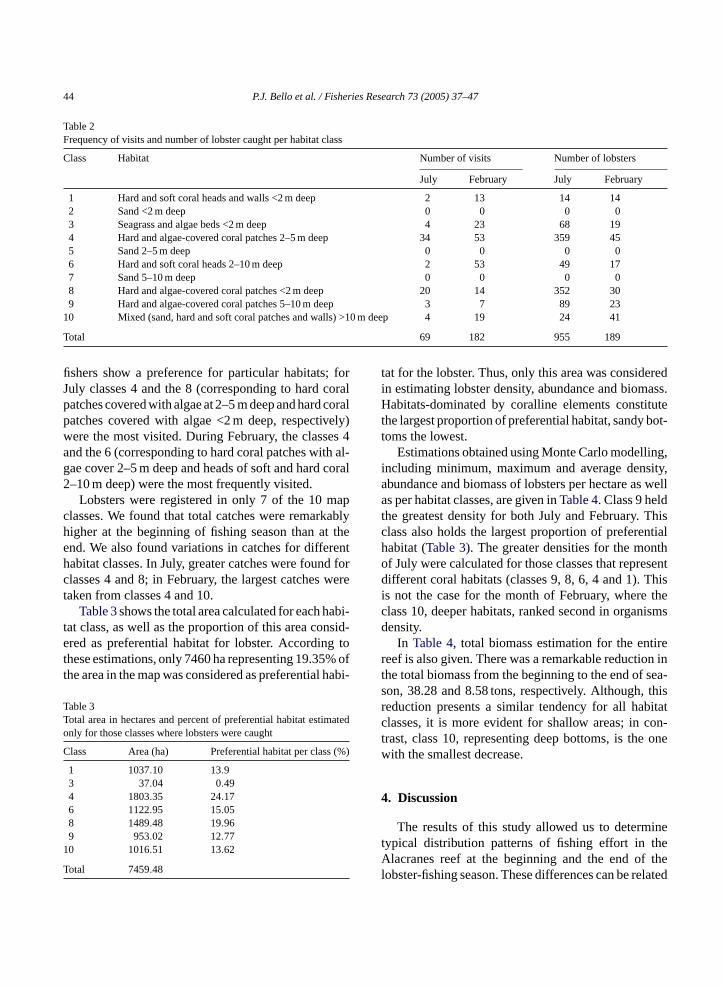
ats map, it was possible to calculate the frequencisits and the number of lobsters caught per habithe beginning and end of fishing season.Table 2sum-arizes those results. It can be observed that lo
44 P.J. Bello et al. / Fisheries Research 73 (2005) 37–47
Table 2Frequency of visits and number of lobster caught per habitat class
Class Habitat Number of visits Number of lobsters
July February July February
1 Hard and soft coral heads and walls <2 m deep 2 13 14 142 Sand <2 m deep 0 0 0 03 Seagrass and algae beds <2 m deep 4 23 68 194 Hard and algae-covered coral patches 2–5 m deep 34 53 359 455 Sand 2–5 m deep 0 0 0 06 Hard and soft coral heads 2–10 m deep 2 53 49 177 Sand 5–10 m deep 0 0 0 08 Hard and algae-covered coral patches <2 m deep 20 14 352 309 Hard and algae-covered coral patches 5–10 m deep 3 7 89 23
10 Mixed (sand, hard and soft coral patches and walls) >10 m deep 4 19 24 41
Total 69 182 955 189
fishers show a preference for particular habitats; forJuly classes 4 and the 8 (corresponding to hard coralpatches covered with algae at 2–5 m deep and hard coralpatches covered with algae <2 m deep, respectively)were the most visited. During February, the classes 4and the 6 (corresponding to hard coral patches with al-gae cover 2–5 m deep and heads of soft and hard coral2–10 m deep) were the most frequently visited.
Lobsters were registered in only 7 of the 10 mapclasses. We found that total catches were remarkablyhigher at the beginning of fishing season than at theend. We also found variations in catches for differenthabitat classes. In July, greater catches were found forclasses 4 and 8; in February, the largest catches weretaken from classes 4 and 10.
Table 3shows the total area calculated for each habi-tat class, as well as the proportion of this area consid-ered as preferential habitat for lobster. According tothese estimations, only 7460 ha representing 19.35% ofthe area in the map was considered as preferential habi-
Table 3Total area in hectares and percent of preferential habitat estimatedonly for those classes where lobsters were caught
Class Area (ha) Preferential habitat per class (%)
1 1037.10 13.93 37.04 0.494 1803.35 24.176 1122.95 15.058 1489.48 19.969 953.02 12.77
1
T
tat for the lobster. Thus, only this area was consideredin estimating lobster density, abundance and biomass.Habitats-dominated by coralline elements constitutethe largest proportion of preferential habitat, sandy bot-toms the lowest.
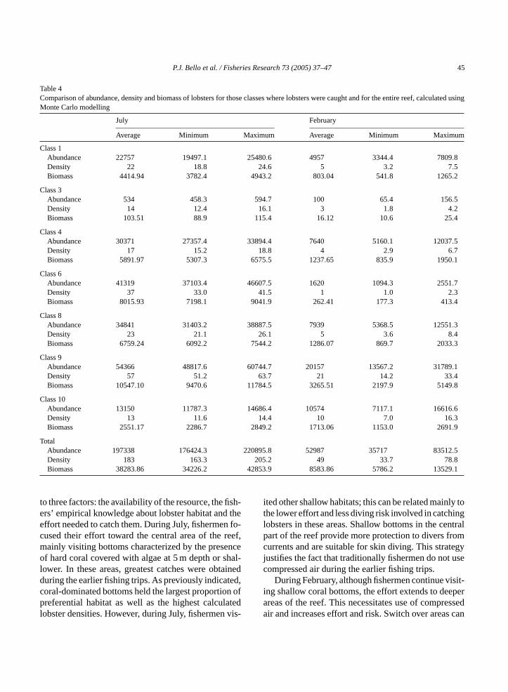
Estimations obtained using Monte Carlo modelling,including minimum, maximum and average density,abundance and biomass of lobsters per hectare as wellas per habitat classes, are given inTable 4. Class 9 heldthe greatest density for both July and February. Thisclass also holds the largest proportion of preferentialhabitat (Table 3). The greater densities for the monthof July were calculated for those classes that representdifferent coral habitats (classes 9, 8, 6, 4 and 1). Thisis not the case for the month of February, where theclass 10, deeper habitats, ranked second in organismsdensity.
In Table 4, total biomass estimation for the entirereef is also given. There was a remarkable reduction inthe total biomass from the beginning to the end of sea-son, 38.28 and 8.58 tons, respectively. Although, thisreduction presents a similar tendency for all habitatclasses, it is more evident for shallow areas; in con-trast, class 10, representing deep bottoms, is the onewith the smallest decrease.
4. Discussion
The results of this study allowed us to determinet heA thel lated
0 1016.51 13.62
otal 7459.48
ypical distribution patterns of fishing effort in tlacranes reef at the beginning and the end of
obster-fishing season. These differences can be re
P.J. Bello et al. / Fisheries Research 73 (2005) 37–47 45
Table 4Comparison of abundance, density and biomass of lobsters for those classes where lobsters were caught and for the entire reef, calculated usingMonte Carlo modelling
July February
Average Minimum Maximum Average Minimum Maximum
Class 1Abundance 22757 19497.1 25480.6 4957 3344.4 7809.8Density 22 18.8 24.6 5 3.2 7.5Biomass 4414.94 3782.4 4943.2 803.04 541.8 1265.2
Class 3Abundance 534 458.3 594.7 100 65.4 156.5Density 14 12.4 16.1 3 1.8 4.2Biomass 103.51 88.9 115.4 16.12 10.6 25.4
Class 4Abundance 30371 27357.4 33894.4 7640 5160.1 12037.5Density 17 15.2 18.8 4 2.9 6.7Biomass 5891.97 5307.3 6575.5 1237.65 835.9 1950.1
Class 6Abundance 41319 37103.4 46607.5 1620 1094.3 2551.7Density 37 33.0 41.5 1 1.0 2.3Biomass 8015.93 7198.1 9041.9 262.41 177.3 413.4
Class 8Abundance 34841 31403.2 38887.5 7939 5368.5 12551.3Density 23 21.1 26.1 5 3.6 8.4Biomass 6759.24 6092.2 7544.2 1286.07 869.7 2033.3
Class 9Abundance 54366 48817.6 60744.7 20157 13567.2 31789.1Density 57 51.2 63.7 21 14.2 33.4Biomass 10547.10 9470.6 11784.5 3265.51 2197.9 5149.8
Class 10Abundance 13150 11787.3 14686.4 10574 7117.1 16616.6Density 13 11.6 14.4 10 7.0 16.3Biomass 2551.17 2286.7 2849.2 1713.06 1153.0 2691.9
TotalAbundance 197338 176424.3 220895.8 52987 35717 83512.5Density 183 163.3 205.2 49 33.7 78.8Biomass 38283.86 34226.2 42853.9 8583.86 5786.2 13529.1
to three factors: the availability of the resource, the fish-ers’ empirical knowledge about lobster habitat and theeffort needed to catch them. During July, fishermen fo-cused their effort toward the central area of the reef,mainly visiting bottoms characterized by the presenceof hard coral covered with algae at 5 m depth or shal-lower. In these areas, greatest catches were obtainedduring the earlier fishing trips. As previously indicated,coral-dominated bottoms held the largest proportion ofpreferential habitat as well as the highest calculatedlobster densities. However, during July, fishermen vis-
ited other shallow habitats; this can be related mainly tothe lower effort and less diving risk involved in catchinglobsters in these areas. Shallow bottoms in the centralpart of the reef provide more protection to divers fromcurrents and are suitable for skin diving. This strategyjustifies the fact that traditionally fishermen do not usecompressed air during the earlier fishing trips.
During February, although fishermen continue visit-ing shallow coral bottoms, the effort extends to deeperareas of the reef. This necessitates use of compressedair and increases effort and risk. Switch over areas can
46 P.J. Bello et al. / Fisheries Research 73 (2005) 37–47
be due to the diminution of the resource in shallow ar-eas. This was evident in the fishing grounds, since inFebruary deep-water habitat classes such as the class9 (less than 5 m of depth) and the class 10 (more than10 m of depth) presented higher densities of lobster.It is important to indicate that because of the diminu-tion of lobster abundance by the end of the season, thelobster catch is not profitable and the effort is turned to-wards catching fish; lobster then becomes an incidentalspecies, constituting only about 5% of the total catch(Rıos et al., 1998b).
To the best of our knowledge, this is one of the firstattempts to incorporate satellite imagery analysis andGIS, for stock assessment of lobster in large area coralreef habitats. Further studies are needed to improve es-timations. Nevertheless, we believe that the potentialof these tools for evaluation of fishing resources wasevident in this study; even considering their use in amoderated way, they allowed us to integrate data ofdifferent sources, and facilitated the display of infor-mation, analysis, calculations and, later, the display ofresults. It also emphasizes the potential implications ofthis approach for management of Alacranes Reef Park.As Green et al. (2000)discussed, correlation betweencoral reef bottoms and the number of lobsters can beused to delineate habitats and improve evaluation ofstock and management of lobster fisheries. We believethat a better understanding of spatial distribution of theresource and fishers effort can facilitate more realis-tic estimations of biological populations and result inb f re-s as af sters stemm bvi-o ta forA n ther catan(
vi-o ssb rent.I otall esv hesf son,e noti size.
Another important point is that if we consider that bythe end of the season, we calculated a total biomass ofonly 8.66 tons, it would be evident that every year mostof available lobster biomass is extracted from the reef,thus, implying that there should be a renewal process ofthe lobster population from February to July. It wouldbe very interesting to continue estimating the biomassfor the following seasons to determine if this is true.
This study was specifically directed to the traditionalfishing areas and some habitats were visited less fre-quently or not visited at all. This might lead to under-estimating an important part of lobster population, andsuggests the need to carry out further studies on lobsterstock assessment considering all habitats, including theless visited fishing areas and also before the fishing sea-son begins. We are aware that the preferential habitatcalculation was a subjective exercise because no formalstudy has been directed specifically for Alacranes reef,but it was supported on habitat characterizations donefor the Caribbean (Childress and Herrnkind, 1996;Herrera and Ibarzabal, 1995; Cruz et al., 1995). It wouldbe of great interest to design studies specifically for thecharacterization of their particular habitats in the reef.
Acknowledgements
We thank the unions of fishermen at Puerto Progresoand J. Carlos Espinoza for their support during field-work, also the anonymous reviewers, who contributedt wl-e udyw xi-c
R
A rama, Yu-
B es,
C l be-hav.
C ,
C rate-coral
etter decisions regarding the management of reeources. In this study, the use of GPS devices wactor key to link data from habitats map and loburveys, bringing them to the same coordinate syade spatial analysis possible. This may sound ous, but in the near past, there were no spatial dalacranes fishing areas and stock assessments o
eef were based on catches landed in Progreso, YuRıos et al., 1998b).
The estimatorR used in this work, was tested preusly byRıos et al. (1995), and was reported to be leiased when the size of the sampled areas was diffe
n our work using this estimator, we calculated a tobster biomass of 38.28 tons for July, which comery close to the 35 tons officially reported as catcor the Alacranes reef during the 1997 fishing seaspecially if we consider that official statistics do
nclude discarded lobsters or lobsters under legal
o improve this paper. P.J. Bello specially acknodges CONACYT for his Ph.D. scholarship. This stas funded by SISIERRA-CONACYT and the Mean National Institute of Fisheries.
eferences
rdisson, H.P., Duncan, J., Aguirre, L., Canela, J., 1996. Progde manejo del Parque Marino Nacional Arrecife Alacranescatan, Mexico, CINVESTAV-IPN, Merida.
onet, F., 1967. Biogeologıa Subsuperficial del arrecife AlacranYucatan. Instituto de Geologıa, UNAM, Boletın 80, 192 pp.
hildress, M.J., Herrnkind, W.F., 1996. The ontogeny of sociahaviour among juvenile Caribbean spiny lobsters. Anim. Be51, 675–687.
huvieco, E., 1990. Fundamentos de teledeteccion espacial. RIALPMadrid, 453 pp.
rosby, M.P., Brighouse, G., Pichon, M., 2002. Priorities and stgies for addressing natural and anthropogenic threats to
P.J. Bello et al. / Fisheries Research 73 (2005) 37–47 47
reefs in Pacific Island Nations. Ocean Coastal Manage. 45,121–137.
Cruz, R., Gonzalez, J., De Leon, M.E., Puga, R., 1995. La pesquerıade langosta espinosa (Panulirus argus) en el Gran Caribe. Eval-uacion y pronostico. Rev. Cub. Inv. Pesq. 19 (2), 63–76.
Davidson, R.J., Villouta, E., Cole, R.G., Barrier, R.G.F., 2002. Ef-fects of marine reserve protection on spiny lobster (Jasus ed-wardsii) abundance and size at Tonga Island Marine Reserve,New Zealand. Aquatic Conserv. Mar. Freshwater Ecosys. 12,213–227.
De la Cruz, G., Martınez, E., Munoz, R., 1993. Propuesta de zonifi-cacion del Arrecife Alacranes, Yucatan, CINVESTAV, Merida.
Digby, P., Kempton, R., 1987. Multivariate Analysis of Communities.Chapman and Hall, London, NewYork.
Done, T., 1981. Rapid, large area, reef resource surveys using amanta board. In: Proceedings of the Fourth International Coralreef Symposium 1, pp. 299–308.
Evans, Ch.R., Evans, A.J., 1996. A practical field technique for theassessment of spiny lobster resources of tropical islands. Fish.Res. 26, 149–169.
Green, E.P., Mumby, P.J., Edwards, A.J., Clark, C.D., 1996. A reviewof remote sensing for assessment and management of tropicalcoastal resources. Coastal Manage. 24, 1–40.
Green, E.P., Mumby, P.J., Edwards, A.J., Clark, C.D. (Eds.), 2000.Coastal Management Sourcebooks 3. UNESCO, Paris, 316 pp.
Herrera, A., Ibarzabal, D., 1995. Aspectos ecologicos de la langostaPanulirus argusen los arrecifes de la plataforma cubana. Rev.Cub. Inv. Pesq. 19 (1), 59–63.
Human, P., 1994. Reef Coral Identification. New World PublicationsInc., Florida, 239 pp.
Jones, R.L., Stoner, A.W., 1997. The integration of GIS and RemoteSensing in an Ecological Study of Queen Conch,Strombus gigas,Nursery Habitats. In: Proceedings of the 49th Gulf and CaribbeanFisheries Institute Congress, pp. 523–530.
Kenchington, R., 1978. Visual surveys of large areas of coral reefs. In:thods.
K ers,
L entso.,
L
Liceaga, C.M.A., Rıos, L.G.V., Zetina, M.C., Hernandez, N.H., 1997.Clasificacion rapida del ambiente arrecifal para la evaluacionde los recursos pesqueros. In: Proceedings of the 50th AnnualGulf and Caribbean Fisheries Institute Congress, pp. 185–189.
Lillesand, T.M., Kiefer, R.W., 1979. Remote Sensing and Image In-terpretation. John Wiley and Sons Ltd., USA, 612 pp.
Magellan Systems Corporation, 1995. Magellan NAV DLX-10 UserGuide. San Dimas, California.
Microimages, 2001. Reference manual for TNT Products V6.8. Lin-coln, NE, USA.
Mumby, P.J., Harborne, A.R., 1999. Development of a systematicclassification scheme of marine habitats to facilitate regionalmanagement and mapping of Caribbean coral reefs. Biol. Con-serv. 88, 155–163.
Mumby, P.J., Green, E.P., Clark, C.D., Edwards, A.J., 1998. Digitalanalysis of multispectral airborne imagery of coral reefs. CoralReefs 17, 59–69.
Rıos, L.G.V., Zetina, M.C., Cervera, C.K., 1995. Evaluacion de “ca-sitas” o refugios artificiales introducidos en la costa oriente delestado de Yucatan para la captura de langosta. Rev. Cub. Inv.Pesq. 19 (2), 50–56.
Rıos, L.G.V., Zetina, M.C., Cervera, C.K., Mena, A.R., Chable, E.F.,1998a. La pesquerıa de langosta espinosaPanulirus argusenla costa de Yucatan. Contribuciones de Investigacion Pesquera.Centro Regional de Investigaciones Pesqueras Yucalpeten. INP.SEMARNAP. Documento Tecnico 6, pp. 1–36.
Rıos, L.G.V., Cervera, C.K., Espinoza, M.J.C., Perez, P.M., Chable,E.F., Zetina, M.C., 1998b. Estimacion de las densidades de lan-gosta espinosa (Panulirus argus) y caracol rosado (Strombus gi-gas) en elarea central del arrecife Alacranes, Yucatan Mexico.In: Proceedings of the 50th Annual Gulf and Caribbean FisheriesInstitute, pp. 104–127.
Rıos, L.G.V., Bello, P.J., Zetina, M.C., Cervera, C.K., Arceo, B.P.,2003. Estimacion de densidad abundancia y biomasa de la
oshe72–
S ward
t spon-ecol-
Stoddart, D., Johannes, R. (Eds.), Coral Reefs Research MeUNESCO, Paris, pp. 149–161.
rebs, C., 1989. Ecological Methodology. Harper Collins PublishUSA.
egendre, L., Legendre, P., 1983. Numerical Ecology. Developmin Environmental Modeling 3. Elsevier Scientific Publishing CNew York.
iceaga, C.M.A., Hernandez, N.H., 2000. Localizacion y dimen-siones del Arrecife Alacranes. Jaina 11, 8–10.
langosta espinosaP. argus en el arrecife Alacranes en lanos 1997–1999 con aplicacion de GIS. In: Proceedings of t54th Annual Gulf and Caribbean Fisheries Institute, pp. 2284.
eber, G.A.F., 1982. The Estimation of Animal Abundance. EdArnold, UK.
er Braak, C.J.F., Verdonschot, P.F.M., 1995. Canonical corredence analysis and related multivariate methods in aquaticogy. Aquatic Sci. 57, 256–286.
Related Documents