Haar waveletsmdav.ece.gatech.edu/ece-6250-fall2017/notes/06-notes-6250-f17.pdf · Haar wavelets The Haar wavelet basis for L2 (R) breaks down a signal by lookingat the di erence between

Haar wavelets

The Haar wavelet basis for L2(R) breaks down a signal by lookingat the difference between piecewise constant approximations at dif-ferent scales. It is the simplest example of a wavelet transform,and is very easy to understand.

Let V0 be the space of signals that are piecewise constant betweenthe integers. Example member:

−2

−1

0

1

2

3

−3 −2 −1 0 1 2 3 4

Set

φ0(t) =

{1 0 ≤ t < 1

0 otherwise−0.5

0

0.5

1

1.5

0 1

It is clear that {φ0(t− n), n ∈ Z} is an orthobasis for V0.

Given an arbitrary x0(t), we can find the best piecewise constant(between the integers) approximation by projecting onto the spanof the {φ0(t− n)}. To keep the notation compact, we use

φ0,n(t) = φ0(t− n),

and then the closest signal in V0 to x(t) is

x̂0(t) =∞∑

n=−∞〈x0,φ0,n〉φ0,n(t).

117

Georgia Tech ECE 6250 Fall 2017; Notes by J. Romberg and M. Davenport. Last updated 1:33, September 25, 2017

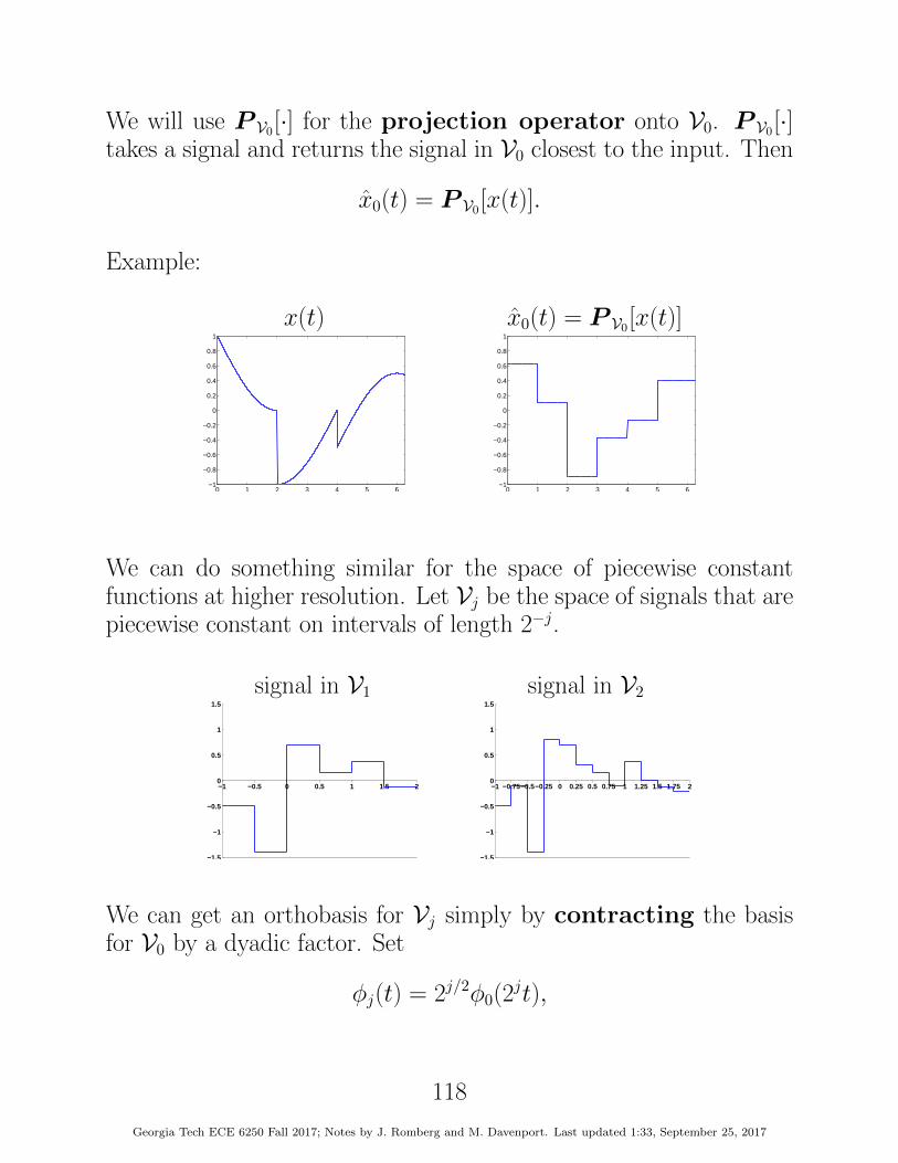
We will use P V0[·] for the projection operator onto V0. P V0[·]takes a signal and returns the signal in V0 closest to the input. Then

x̂0(t) = P V0[x(t)].

Example:

x(t) x̂0(t) = P V0[x(t)]

0 1 2 3 4 5 6−1

−0.8

−0.6

−0.4

−0.2

0

0.2

0.4

0.6

0.8

1

0 1 2 3 4 5 6−1

−0.8

−0.6

−0.4

−0.2

0

0.2

0.4

0.6

0.8

1

We can do something similar for the space of piecewise constantfunctions at higher resolution. Let Vj be the space of signals that arepiecewise constant on intervals of length 2−j.

signal in V1 signal in V2

−1.5

−1

−0.5

0

0.5

1

1.5

−1 −0.5 0 0.5 1 1.5 2

−1.5

−1

−0.5

0

0.5

1

1.5

−1 −0.75−0.5−0.25 0 0.25 0.5 0.75 1 1.25 1.5 1.75 2

We can get an orthobasis for Vj simply by contracting the basisfor V0 by a dyadic factor. Set

φj(t) = 2j/2φ0(2jt),

118


andφj,n(t) = φj(t− 2−jn) = 2j/2φ0(2

jt− n).

Then it is easy to see that

{φj,n(t), n ∈ Z}is an orthobasis for Vj.

Examples:

φ1,−1(t)

φ1,0(t)

φ1,1(t)

φ1,2(t)

−1 −0.5 0 0.5 1 1.5 20

0.51

1.5

−1 −0.5 0 0.5 1 1.5 20

0.51

1.5

−1 −0.5 0 0.5 1 1.5 20

0.51

1.5

−1 −0.5 0 0.5 1 1.5 20

0.51

1.5

−1 −0.5 0 0.5 1 1.5 2012

−1 −0.5 0 0.5 1 1.5 2012

−1 −0.5 0 0.5 1 1.5 2012

−1 −0.5 0 0.5 1 1.5 2012

−1 −0.5 0 0.5 1 1.5 2012

−1 −0.5 0 0.5 1 1.5 2012

−1 −0.5 0 0.5 1 1.5 2012

−1 −0.5 0 0.5 1 1.5 2012

φ2,−2(t)

φ2,−1(t)

φ2,0(t)

φ2,1(t)

φ2,2(t)

φ2,3(t)

φ2,4(t)

φ2,5(t)

The best approximation to an arbitrary signal x(t) ∈ L2(R) is againgiven by

x̂j(t) = P Vj [x(t)] =∞∑

n=−∞〈x,φj,n〉φj,n(t)

As j increases this approximation becomes better and better:

119


x(t) x̂0(t) (in V0)

0 1 2 3 4 5 6−1

−0.8

−0.6

−0.4

−0.2

0

0.2

0.4

0.6

0.8

1

0 1 2 3 4 5 6−1

−0.8

−0.6

−0.4

−0.2

0

0.2

0.4

0.6

0.8

1

x̂1(t) (in V1) x̂2(t) (in V2)

0 1 2 3 4 5 6−1

−0.8

−0.6

−0.4

−0.2

0

0.2

0.4

0.6

0.8

1

0 1 2 3 4 5 6−1

−0.8

−0.6

−0.4

−0.2

0

0.2

0.4

0.6

0.8

1

x̂3(t) (in V3) x̂4(t) (in V4)

0 1 2 3 4 5 6−1

−0.8

−0.6

−0.4

−0.2

0

0.2

0.4

0.6

0.8

1

0 1 2 3 4 5 6−1

−0.8

−0.6

−0.4

−0.2

0

0.2

0.4

0.6

0.8

1

In the end, at “infinitely fine” resolution, we get the original signalback:

limj→∞

x̂j(t) = limj→∞

P Vj [x(t)] = x(t).

The Haar wavelet basis represents the differences between theseapproximations. Set

W0 = V1 V0.This is the space of signals that are in V1 but are orthogonal toeverything in V0. Signals in W0 are piecewise constant between the

120


half integers (just like everything else in V1) but also have zero meanbetween the integers. Example member of W0:

0 1 2 3 4 5 6−1

−0.8

−0.6

−0.4

−0.2

0

0.2

0.4

0.6

0.8

1

Similarly, we can setWj = Vj+1 Vj.

We can generate an orthobasis for the Wj using the following func-

tion: ψ0(t) =

1 0 ≤ t < 1/2

−1 1/2 ≤ t < 1

0 otherwise

.

−1.5

−1

−0.5

0

0.5

1

1.5

0 0.5 1

With

ψj(t) = 2j/2ψ(2jt), ψj,n(t) = ψj(t− 2−jn) = 2j/2ψ0(2jt− n),

then{ψj,n(t), n ∈ Z}

is an orthobasis for Wj.

We now have the following multiscale decomposition for an arbitrary

121


x(t):

x(t) = P V0[x(t)] + PW0[x(t)]︸︷︷︸

=P V1 [x(t)]

+PW1[x(t)]

︸︷︷︸=P V2 [x(t)]

+PW2[x(t)]

︸︷︷︸=P V3 [x(t)]

+ · · ·

The corresponding reproducing formula for the Haar wavelet sys-tem is

x(t) =∞∑

n=−∞〈x,φ0,n〉φ0,n(t)︸︷︷︸=P V0 [x(t)]

+∞∑j=0

∞∑n=−∞〈x,ψj,n〉ψj,n(t)︸︷︷︸=PWj

[x(t)]

Here are plots of the φj,n(t) and ψj,n(t) at the first three scales:

(From Burrus et al, Intro. to Wavelets and Wavelet Transforms)

122


Nomenclature

• We call the Vj the scaling spaces or approximation spaces.

• The {φj,n, n ∈ Z} are an orthobasis for Vj, and are calledscaling functions at scale j.

• The Wj are called wavelet spaces or detail spaces.

• The {ψj,n(t), n ∈ Z} are an orthobasis for Wj, and are calledwavelets at scale j.

• The expansion coefficients that specify the approximation x̂j

in terms of the φj,n are called scaling coefficients: in theexpression

x̂j =∞∑

n=−∞sj,n φj,n(t), sj,n = 〈x,φj,n〉,

the sj,n are scaling coefficients at scale j.

• The expansion coefficients for the projection ontoWj are calledwavelet coefficients wj,n at scale j:

wj,n = 〈x,ψj,n〉,

and

PWj[x(t)] =

∞∑n=−∞

wj,n ψj,n(t).

123


Moving between scales

We have seen that conceptually, the Haar transform analyzes a sig-nal through a series of multiscale approximations onto nestedsubspaces Vj, with

V0 ⊂ V1 ⊂ V2 ⊂ · · · ⊂ L2(R).

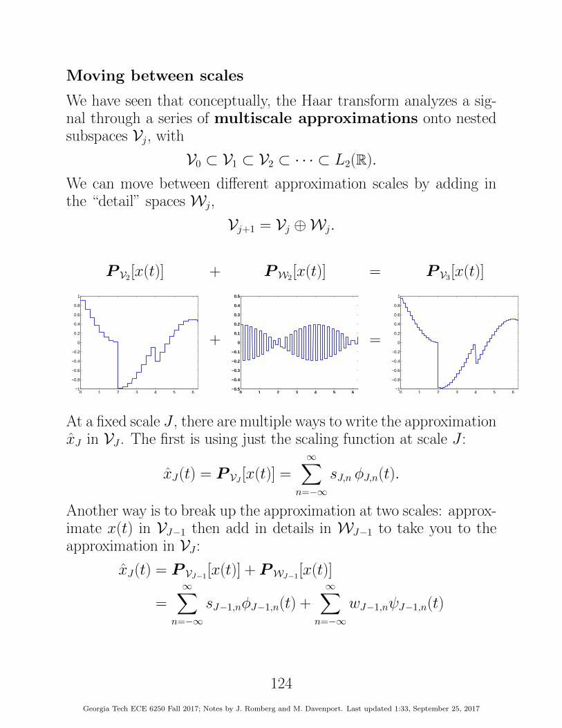
We can move between different approximation scales by adding inthe “detail” spaces Wj,

Vj+1 = Vj ⊕Wj.

P V2[x(t)] + PW2[x(t)] = P V3[x(t)]

0 1 2 3 4 5 6−1

−0.8

−0.6

−0.4

−0.2

0

0.2

0.4

0.6

0.8

1

+

0 1 2 3 4 5 6−0.5

−0.4

−0.3

−0.2

−0.1

0

0.1

0.2

0.3

0.4

0.5

=

0 1 2 3 4 5 6−1

−0.8

−0.6

−0.4

−0.2

0

0.2

0.4

0.6

0.8

1

At a fixed scale J , there are multiple ways to write the approximationx̂J in VJ . The first is using just the scaling function at scale J :

x̂J(t) = P VJ [x(t)] =∞∑

n=−∞sJ,n φJ,n(t).

Another way is to break up the approximation at two scales: approx-imate x(t) in VJ−1 then add in details in WJ−1 to take you to theapproximation in VJ :

x̂J(t) = P VJ−1[x(t)] + PWJ−1[x(t)]

=∞∑

n=−∞sJ−1,nφJ−1,n(t) +

∞∑n=−∞

wJ−1,nψJ−1,n(t)

124


Yet another way is to break up the approximation at three scales:approximate x(t) in VJ−2, then add in the details in WJ−2 to takeyou to the approximation in VJ−1, then add in the details in WJ−1to take you to the approximation in VJ :

x̂J(t) = P VJ−2[x(t)] + PWJ−2[x(t)] + PWJ−1[x(t)].

Of course we could continue this all the way up to scale 0:

x̂J(t) = P V0[x(t)] + PW0[x(t)] + · · · + PWJ−1[x(t)]

=∞∑

n=−∞s0,nφ0,n(t) +

J−1∑j=0

∞∑n=−∞

wj,nψj,n(t).

One of the key properties of the Haar wavelet transform (and allwavelet transforms, as we will see later) is that there is an efficientway to compute the multiscale approximation coefficients{s0,n, w0,n, w1,n, . . . , wJ−1,n} from the single scale approximationcoefficients {sJ,n}.

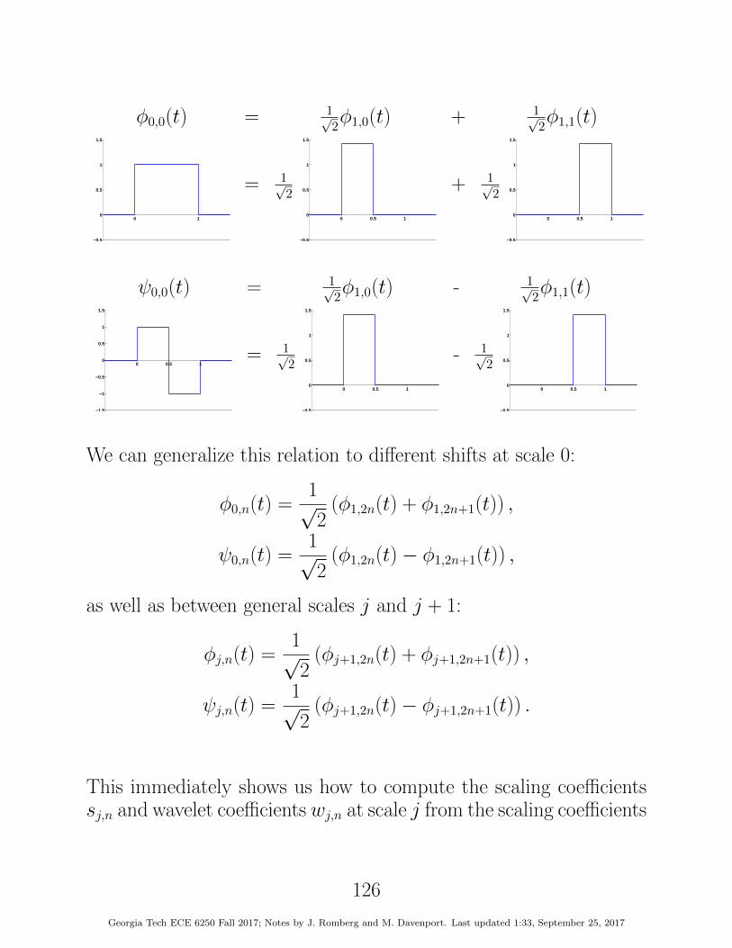
What lets us do this is the simple fact that the scaling functionsφJ−1,n and wavelet functions ψJ−1,n at scale J − 1 both can be builtup out of scaling functions φJ,n at scale J . To start, let us look atscale V1 = V0 ⊕W0. Now, as we illustrate below,

φ0(t) =1√2

(φ1(t) + φ1(t− 1/2)) ,

=1√2

(φ1,0(t) + φ1,1(t)) ,

and

ψ0(t) =1√2

(φ1,0(t)− φ1,1(t)) .

125


φ0,0(t) = 1√2φ1,0(t) + 1√

2φ1,1(t)

−0.5

0

0.5

1

1.5

0 1

= 1√2

−0.5

0

0.5

1

1.5

0 0.5 1

+ 1√2

−0.5

0

0.5

1

1.5

0 0.5 1

ψ0,0(t) = 1√2φ1,0(t) - 1√

2φ1,1(t)

−1.5

−1

−0.5

0

0.5

1

1.5

0 0.5 1= 1√

2

−0.5

0

0.5

1

1.5

0 0.5 1

- 1√2

−0.5

0

0.5

1

1.5

0 0.5 1

We can generalize this relation to different shifts at scale 0:

φ0,n(t) =1√2

(φ1,2n(t) + φ1,2n+1(t)) ,

ψ0,n(t) =1√2

(φ1,2n(t)− φ1,2n+1(t)) ,

as well as between general scales j and j + 1:

φj,n(t) =1√2

(φj+1,2n(t) + φj+1,2n+1(t)) ,

ψj,n(t) =1√2

(φj+1,2n(t)− φj+1,2n+1(t)) .

This immediately shows us how to compute the scaling coefficientssj,n and wavelet coefficientswj,n at scale j from the scaling coefficients

126


sj+1,n at scale j + 1:

sj,n = 〈x,φj,n〉=

1√2〈x,φj+1,2n〉 +

1√2〈x,φj+1,2n+1〉

=1√2sj+1,2n +

1√2sj+1,2n+1,

and

wj,n = 〈x,ψj,n〉=

1√2〈x,φj+1,2n〉 −

1√2〈x,φj+1,2n+1〉

=1√2sj+1,2n −

1√2sj+1,2n+1.

If we think of the scaling/wavelet coefficients at scale j as a discretetime sequence, so sj[n] := sj,n andwj[n] := wj,n, then the expressionsabove suggest that the scaling coefficients at scale j can be brokendown scaling and wavelet coefficients at scale j−1 using the followingarchitecture:

2

2

sj+1[n]

sj [n]

wj [n]

h0[n]

h1[n]

127


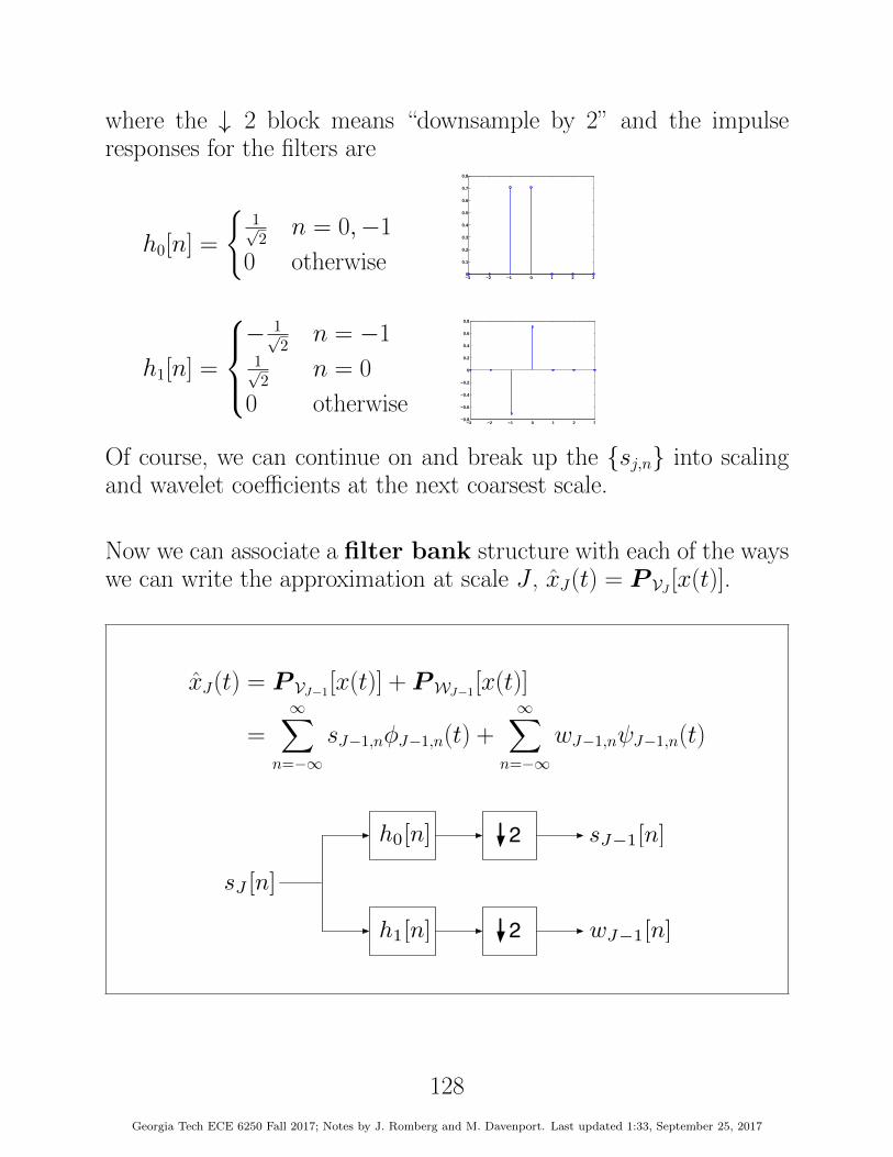
where the ↓ 2 block means “downsample by 2” and the impulseresponses for the filters are

h0[n] =

{1√2

n = 0,−1

0 otherwise

h1[n] =

− 1√

2n = −1

1√2

n = 0

0 otherwise

−3 −2 −1 0 1 2 30

0.1

0.2

0.3

0.4

0.5

0.6

0.7

0.8

−3 −2 −1 0 1 2 3−0.8

−0.6

−0.4

−0.2

0

0.2

0.4

0.6

0.8

Of course, we can continue on and break up the {sj,n} into scalingand wavelet coefficients at the next coarsest scale.

Now we can associate a filter bank structure with each of the wayswe can write the approximation at scale J , x̂J(t) = P VJ [x(t)].

x̂J(t) = P VJ−1[x(t)] + PWJ−1[x(t)]

=∞∑

n=−∞sJ−1,nφJ−1,n(t) +

∞∑n=−∞

wJ−1,nψJ−1,n(t)

2

2

h0[n]

h1[n]

sJ [n]

sJ�1[n]

wJ�1[n]

128


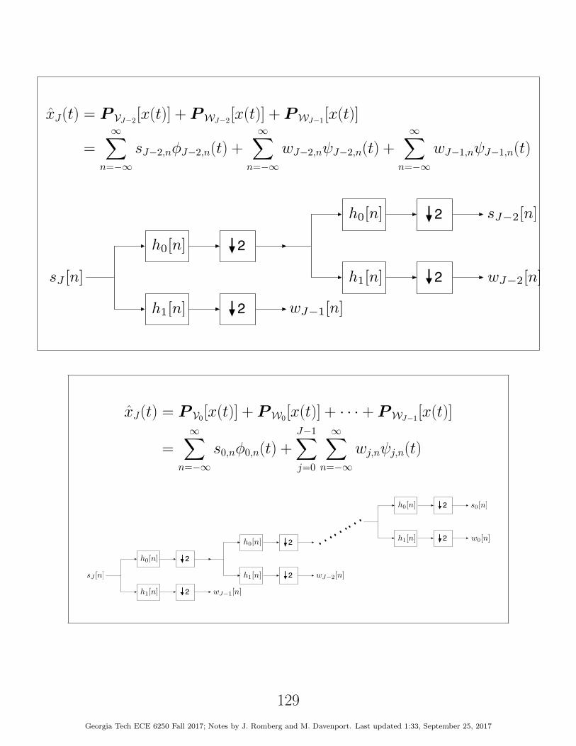
x̂J(t) = P VJ−2[x(t)] + PWJ−2[x(t)] + PWJ−1[x(t)]

=∞∑

n=−∞sJ−2,nφJ−2,n(t) +

∞∑n=−∞

wJ−2,nψJ−2,n(t) +∞∑

n=−∞wJ−1,nψJ−1,n(t)

2

2

h0[n]

h1[n]

sJ [n]

sJ�2[n]2

2

h0[n]

h1[n] wJ�2[n]

wJ�1[n]

x̂J(t) = P V0[x(t)] + PW0[x(t)] + · · · + PWJ−1[x(t)]

=∞∑

n=−∞s0,nφ0,n(t) +

J−1∑j=0

∞∑n=−∞

wj,nψj,n(t)

2

2

h0[n]

h1[n]

sJ [n]

s0[n]

2

2

h0[n]

h1[n]

· · ·2

2

h0[n]

h1[n]· · ·· · · w0[n]

wJ�1[n]

wJ�2[n]

129


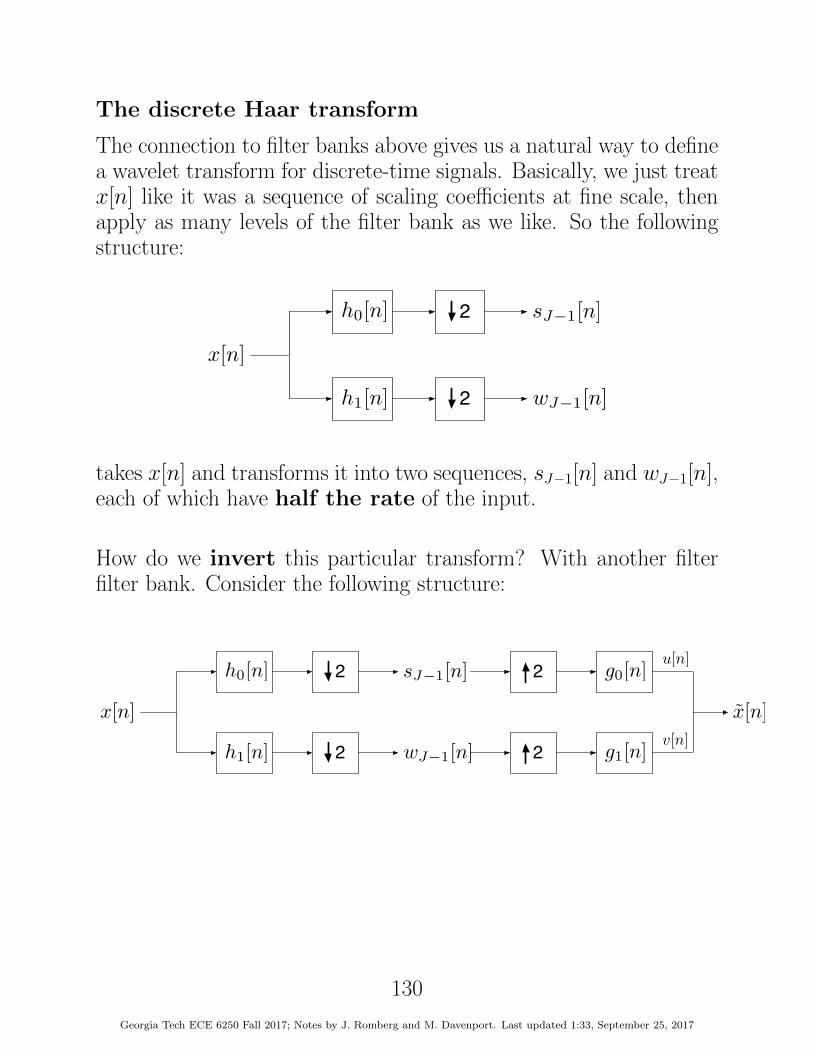
The discrete Haar transform

The connection to filter banks above gives us a natural way to definea wavelet transform for discrete-time signals. Basically, we just treatx[n] like it was a sequence of scaling coefficients at fine scale, thenapply as many levels of the filter bank as we like. So the followingstructure:

2

2

h0[n]

h1[n]

sJ�1[n]

wJ�1[n]

x[n]

takes x[n] and transforms it into two sequences, sJ−1[n] and wJ−1[n],each of which have half the rate of the input.

How do we invert this particular transform? With another filterfilter bank. Consider the following structure:

2

2

h0[n]

h1[n]

sJ�1[n]

wJ�1[n]

x[n]

2

2

x̃[n]

g0[n]

g1[n]

u[n]

v[n]

130


If we take

g0[n] = h0[−n] =

{1√2

n = 0, 1

0 otherwise

g1[n] = h1[−n] =

1√2

n = 0

− 1√2

n = 1

0 otherwise

,

then we will have x̃[n] = x[n]. To see this, recall that

sJ−1[n] =1√2

(x[2n] + x[2n + 1]),

and so

u[n] =

{12

(x[n] + x[n + 1]) n even12

(x[n− 1] + x[n]) n odd,

that is, the values in u[n] appear in pairs,

u[0] = u[1] =1

2(x[0] + x[1]), u[2] = u[3] =

1

2(x[2] + x[3]), etc.

Similarly, since

wJ−1[n] =1√2

(x[2n]− x[2n + 1]) ,

we have

v[n] =

{12

(x[n]− x[n + 1]) n even12

(−x[n− 1] + x[n]) n odd,

that is, the values in v[n] appear in pairs of ± terms,

v[0] = −v[1] =1

2(x[0]− x[1]), v[2] = −v[3] =

1

2(x[2]− x[3]), etc.

131


Now it is easy to see that

x̃[n] = u[n] + v[n] = x[n] for all n ∈ Z.

We can repeat this to as many levels as we desire. For example, thefollowing structure

2

2

h0[n]

h1[n] wJ�1[n]

x[n]

2

2

h0[n]

h1[n] wJ�2[n]

sJ�2[n]

takes x[n] and transforms it into three sequences, one of which is athalf the rate of x[n], and the other two are at a quarter of the rate.To invert it, we simply apply the inverse filter bank twice:

wJ�1[n]

2

2

g0[n]

g1[n]

2

2

g0[n]

g1[n]

sJ�2[n]

wJ�2[n] x[n]

It should be clear how to extend this to an arbitrary number of levels.

132


Haar waveletsmdav.ece.gatech.edu/ece-6250-fall2017/notes/06-notes-6250-f17.pdf · Haar wavelets The Haar wavelet basis for L2 (R) breaks down a signal by lookingat the di erence between

Documents