H L M A 2010 H M A Study of Infectious Diseases Through ...

Hang Lung Mathematics AwardsVol. 4 (2010)

HANG LUNG MATHEMATICS AWARDS 2010

HONORABLE MENTION

A Study of Infectious Diseases Through

Mathematical Modeling

Team Members: On Ping Chung, Winson Che Shing Li, Hon Kei Lai,Wing Yan Shiao, Sung Him Wong

Teacher: Mr. Wing Kwong WongSchool: Hong Kong Chinese Women’s Club College

Hang Lung Mathematics Awards c© 2010, IMS, CUHKVol. 4 (2010), pp. 111–163

A STUDY OF INFECTIOUS DISEASES BY MATHEMATICAL

MODELS

TEAM MEMBERS

On Ping Chung, Winson Che Shing Li, Hon Kei Lai,Wing Yan Shiao, Sung Him Wong

TEACHER

Mr. Wing Kwong Wong

SCHOOL

Hong Kong Chinese Women’s Club College

Abstract. Diseases are devastating. The SARS in 2003 and the swine in-

fluenza in 2009 sparked myriad of questions in our minds. Our major concern

is the spread of germs. Throughout the entire project, we investigate disease-related issues and try to study the impacts of a disease by mathematical mod-

eling.

We first start with the simplest model followed by more complicated ones.We focus on different factors that affect the spread of diseases. Diagrams are

included in each chapter to see how the values of different groups vary. Then

we come up with possible ways to prevent epidemics. Altering the models byadding more conditions, we find one that fits the real life situation - the SEIRS

model. The situation in Hong Kong (Swine Influenza from April 2009 to April2010 in Hong Kong) is simulated by putting the data into the model and ourgoal is fulfilled.

Introduction

Diseases had been bothering us for hundreds and thousands of years. Casualties,social destruction and havoc are the possible consequences. Pandemics were justas devastating as natural disasters, no matter when it occurred. Plague caused thedeath of 25 million people from 541 to 542 while Black Death was estimated to kill75 million people. In the last century, about 50 million people were dead becauseof the Spanish flu. What a shocking number!

The spread of the above pandemics took place centuries ago. Is there any thathappened in recent years? In 2003, there was an outbreak of SARS (Severe acuterespiratory syndrome) all over the world, causing panic among the public. 8273people were infected from November 2002 to July 2003. The mortality rate was

111

112 O.P. CHUNG, WINSON LI, H.K. LAI, W.Y. SHIAO, S.H. WONG

pretty high, reaching 9.6%. Apart from this, there was a widespread of swineinfluenza in 2009. Although the fatality rate was not as high as what we had firstpredicted, this aroused our awareness of public health.

If there is a remedy for all the diseases, then we will no longer be fearful of them.However, there may not be cure for some fatal diseases in reality. The occurrence ofthe above incidents sparked myriad of questions in our minds. We are deeply con-cerned about how a disease spreads. What are the factors influencing the outbreakof diseases? Are there any measures that are essential to prevent the widespread ofdisease? What is the most effective and advisable way to deal with the outbreakof diseases? Intrigued by this topic, we hope we can come up with answers to ourqueries in our project by mathematical means.

Throughout the project, we look into disease-related issues. We try to investigatethe effects of a disease by mathematical modeling. In the meantime, we will find outthe factors affecting the spread of diseases and possible ways to prevent epidemics.Additionally, data will be put in the model to simulate the situation in Hong Kong.Altering the models, we are longing for one that fits well in the real life situation.We hope we will be able to find out the rate of being infected and recovery and thenumber of people to be infected or should be vaccinated, etc. by substituting data.Our ultimate goal is to study how an disease spreads.

In the first chapter, we start with the simplest case – the SI model, with onlysusceptible group and infective model. We find that the results obtained do notcomply with data of our daily lives. This prompts us to modify the model. So theSIS and SIR models are discussed in Chapter 3 and 4. As we know, a daily lifesituation can be very complicated with lots of variables. Apart from the suscep-tible, infective and removed group, other people may play a significant role too.That’s why we introduce other elements in the model — SIVD, SIRS, SISR, TSIR,SEIR and SEIRS. In each section, we will first give a definition of all the variableswe use and a detailed explanation of each model. A diagram will be shown toillustrate the idea lucidly. Then we will set the differential equations derived fromthe model. After that, we analyze the equations and see if we can obtain usefulresults. Substituting suitable values of the variables, we will plot graphs to observethe relationship between them. Finally, we will come up with a conclusion basedon the observation.

Last but not least, we cannot finish the project without the help of our school’steachers, Mr. Wong and Mr. Cheung. They have guided and supervised us. Wewould like to acknowledge for their support.

A STUDY OF INFECTIOUS DISEASES BY MATHEMATICAL MODELS 113

1. Background

In this report, we would like to study how diseases are spread in a region. Throughthe investigation, we want to find out how the germs are spread, so as to find a wayto reduce its damage to the society.

Through using differential equation and numerical simulation, we may figure outhow the diseases are spread in the population. For instance, differential equationsare used in Chapter 2 - The SI model.

Differential Equation:

dS

dt= −βSI, dI

dt= βSI (2.1)

With the initial condition I(0) = 1, we can solve the differential equation (2.1).

I =N

1 + (N − 1)e−βSI, S =

N(N − 1)e−βSI

1 + (N − 1)e−βSI(2.2)

Then, we can plot the graph by using Excel with some t and defined β.

For example, S = 6999999, I = 1, N = 7000000 at time 0, and β = 10−7.

Time S I N0 6999999 1 70000001 6999997.986 2.013752 70000002 6999991.834 4.055198 70000003 6999983.555 8.166162 7000000

...

Numerical simulation:

We consider the same case,

dS

dt= −βSI, dI

dt= βSI (2.1)

We consider the rate of change of S and I and take ∆t = 1 day.

So I(t+ ∆t) = I(t) + βS(t)I(t)∆t

I(t+ 1) = I(t) + βS(t)I(t) (2.3)

Also S(t+ ∆t) = β(t)− βS(t)I(t)∆t

S(t+ 1) = S(t)− βS(t)I(t)

For example, S = 6999999, I = 1, N = 7000000 at time 0, and β = 10−7.


I(0)

= 1 (defined)

I(1)

= I(0 + 1)

= I(0) + (10−7)S(0)I(0)

= 1 + (10−7)(6999999)(1)

= 1.70

I(2)

= I(1 + 1)

= I(1) + (10−7)S(1)I(1)

= 1.70 + (10−7)(6999998.3)(1.70)

= 2.89

I(3)

= I(2 + 1)

= I(2) + (10−7)S(2)I(2)

= 2.89 + (10−7)(6999997.11)(2.89)

= 4.913

S(0)

= 6999999

S(1)

= S(0 + 1)

= S(0)− (10−7)(6999999)(1)

= 6999998.3

S(2)

= S(1 + 1)

= S(1)− (10−7)S(1)I(1)

= 6999998.3− (10−7)(6999998.3)(1.7)

= 6999997.11

S(3)

= S(2 + 1)

= S(2)− (10−7)S(2)I(2)

= 6999997.11− (10−7)(6999997.11)(2.89)

= 6999995.087

Etc.

Then we can draw a table.

Time S I N0 6999999 1 70000001 6999998.3 1.7 70000002 6999997.11 2.89 70000003 6999995.087 4.913 7000000

...

Then we can use these data to plot a graph with Excel.

These two methods have similar results and are used throughout our report fre-quently.


There are some similar projects done by other researchers. For example, DavidSmith and Lang Moore have done a project called “The SIR Model for Spread ofDisease”. [See reviewer’s comment (3)] In this project, they are able to create amodel of how Hong Kong flu is spread in New York City in 1968-1969. The modelthey used is SIR model, which will also be discussed in our project.

Symbols will not be mentioned in this section as they are independent in eachmodel.

2. The SI Model

[See reviewer’s comment (2)]

The SI model is the simplest model of an infectious disease which categorizes peopleas either susceptible (S) or infective (I). A susceptible person can become infectiveby contact with an infective. Let β∆t be the probability of a susceptible personbeing infected by an infectious person in time interval ∆t. So,

dS

dt= −βSI, dI

dt= βSI (2.1)

Since there are βSI∆t people moving out from S in ∆t (S is decreasing), we put a“-” sign before βSI. On the other hand, there are βSI∆t people being infected in

∆t (I is increasing) sodI

dtis positive.

SβSI−−→ I

We defined the arrow (−→) as flow of population from one side to another. Hereit means that there are βSI∆t people moving from S to I in ∆t .

We assume that when t = 0, only 1 people is infective and other people is susceptible(i.e. S = 6999999, I = 1).

By solving (2.1) with initial condition I(0) = 1 [See reviewer’s comment (4)]

I =N

1 + (N − 1)e−βSI, S =

N(N − 1)e−βSI

1 + (N − 1)e−βSI(2.2)

We assumed that the population size (N) are 7, 000, 000. We also define thatS+ I = N , which is a constant, at any time t. These assumptions will also be usedin the following chapters. Assuming that the people are well-mixed, meaning thatthey have an equal probability of meeting every person in the population.

Below are some cases of how S and I behave when time goes on.


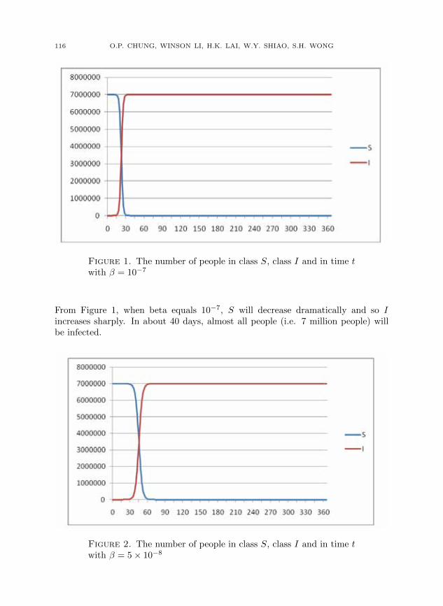
Figure 1. The number of people in class S, class I and in time twith β = 10−7

From Figure 1, when beta equals 10−7, S will decrease dramatically and so Iincreases sharply. In about 40 days, almost all people (i.e. 7 million people) willbe infected.

Figure 2. The number of people in class S, class I and in time twith β = 5× 10−8


From Figure 2, when beta equals 5 × 10−8, S will decrease slightly slower and soI increases in the same rate. In about 90 days, almost all people (i.e. 7 millionpeople) will be infected.

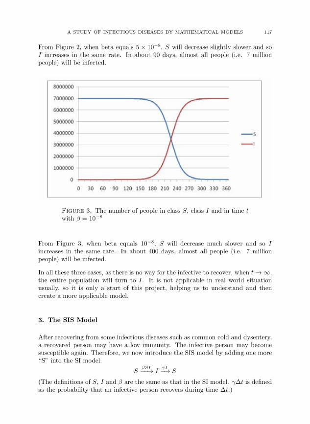
Figure 3. The number of people in class S, class I and in time twith β = 10−8

From Figure 3, when beta equals 10−8, S will decrease much slower and so Iincreases in the same rate. In about 400 days, almost all people (i.e. 7 millionpeople) will be infected.

In all these three cases, as there is no way for the infective to recover, when t→∞,the entire population will turn to I. It is not applicable in real world situationusually, so it is only a start of this project, helping us to understand and thencreate a more applicable model.

3. The SIS Model

After recovering from some infectious diseases such as common cold and dysentery,a recovered person may have a low immunity. The infective person may becomesusceptible again. Therefore, we now introduce the SIS model by adding one more“S” into the SI model.

SβSI−−→ I

γI−→ S

(The definitions of S, I and β are the same as that in the SI model. γ∆t is definedas the probability that an infective person recovers during time ∆t.)


Susceptible people are infected during time ∆t is given by βSI∆t and the infectivepeople who recover during time ∆t is given by γI∆t, i.e.

I(t+ ∆t) = I(t) + βS(t)I(t)∆t− γI(t)∆t

S(t+ ∆t) = S(t)− βS(t)I(t)∆t+ γI(t)∆t

When ∆t→ 0,dI

dt= βSI − γI (3.1)

dS

dt= γI − βSI

Let N be the population size and N = S + I. Define the basic reproductive ratioas

<0 =βN

γ.

We now need to find out the value of I by solving (3.1). Before that we make someassumptions first. We let I0 and S0 be the number of initial infective individualsand initial susceptible individuals respectively. Moreover, we assume I0 = 1. SinceS0 should be much larger than I0, we assume S0 ≈ N . We have the following twocases:

(i) For <0 =βN

γ6= 1,

I =

1

N

(1− 1

<0

) +

1− 1

N

(1− 1

<0

)

e−βN

(1−

1

<0

)t

−1

(3.2)

(ii) For <0 = 1,

I =1

βt+ 1(3.3)

After solving for I, we have to think about whether the disease will spread out at thebeginning and whether the disease will come to an equilibrium position. It is easy

to see that the disease will spread out if I is increasing, i.e.dI

dt> 0. By equation

(3.1) and our assumption S0 ≈ N , the disease will spread out ⇐⇒ <0 > 1.Likewise, the disease will not spread out ⇐⇒ <0 ≤ 1. Therefore, we consider thefollowing two cases:

(i) <0 > 1, the disease will spread out at the beginning.Taking limits on both sides of equation (3.2) as t→∞.

limt→∞

I = N

(1− 1

<0

)


This indicates that when <0 > 1, the disease will spread out and the final

number of infected people will be closed to N

(1− 1

<0

).

(ii) <0 ≤ 1, the disease will not spread out at the beginning.For <0 6= 1, take limits on both sides of equation (3.2) as t→∞.For <0 = 1, take limits on both sides of equation (3.3) as t→∞.Both the above equations show that lim

t→∞I = 0.

This indicates that when <0 ≤ 1, the disease will disappear.

In Hong Kong, the total number of people is around 7 millions. We assume N =7× 106 and β = 10−7. Here, we want to study how the change in γ affects I. Fromthe above results, the disease will spread out when <0 > 1 ⇐⇒ γ < 0.7. On theother hand, the disease will disappear when <0 ≤ 1 ⇐⇒ γ ≥ 0.7. Now we use twographs for illustration.

Figure 4. The number of people in class S, class I in time t withγ = 0.8

Since <0 = 0.875 < 1, the disease will not spread out. The line of I levels off sothe disease will disappear. This is due to the rate of recovery which is greater thanthe rate of being infected.


Figure 5. The number of people in class S, class I in time t withγ = 0.5

Since <0 = 1.4 > 1, the disease will spread out. During 1st to 60th day, I increasesslowly. During 60th to 90th day, I increases dramatically. After 90th day, I becomes

stable and the final number of infected people is around 7×106(

1− 1

1.4

)= 2 mil-

lions. During this period, the rate of recovery equals the rate of being infected.

Conclusion:

If we want the disease to disappear, we have to make <0 less than or equal to 1.Under the condition that β and N are fixed, γ should be maximized. The medicineused to treat the disease can increase the rate of recovery, i.e. increase γ. The SISmodel still has some limitations because the number of infected people will keepconstant (reach the equilibrium position) after some time. This certainly does notmatch with the real situation.

4. The SIR Model

In the SIR model, people are categorized into three groups: the susceptible group,the infective group and the removed group. The people in the susceptible group willbecome infective if they contact people who are infective. Sometimes, the infectivepeople die or are vaccinated. They are not susceptible or infective anymore. In thiscase, we call these group ‘removed’.

SβSI−−→ I

γI−→ R


(The definitions of S, I and β are the same as mentioned in the previous chapters.)

In this chapter, R is the number of people in the removed group and γ is theprobability that one random infective person becomes removed.

We can set three differential equations:

dS

dt= −βSI dI

dt= βSI − γI dR

dt= γI

Now, we define the basic reproductive ratio as

<0 =βN

γ(4.1)

When will an epidemic occur?

For convenience, let S, I and R be the fraction of group S, I and R in the wholepopulation respectively and we take γ−1 as time. [See reviewer’s comment (5)]

S =S

NI =

I

NR =

R

Nt = γt (4.2)

dS

dt= −<0SI

dI

dt= <0SI − I

dR

dt= I

An epidemic will occur if the percentage of infective group is keep on increasing,

i.e.dI

dt= I(<0S − 1), <0S − 1 > 0 with S ≈ S0 (4.3)

By (4.1) and (4.2),

βS0

γ> 1 (4.4)

We can know whether there will be an epidemic by substituting β, γ and S0 into(4.4).

We have another question: What is the least number of people that have to bevaccinated if we want to prevent the epidemics?

Let p be the fraction of people that has to be vaccinated in order to prevent epi-demics. The vaccinated people belong to the removed group.

The fraction of people in the susceptible group is therefore 1− p, i.e. S = 1− p.

By (4.3),<0(1− p) > 1


By calculation,

p < 1− 1

<0(4.5)

An epidemic will occur if p satisfies (4.5).

Therefore, to prevent an epidemic, the least value of p = 1− 1

<0.

In this chapter, we want to study the change in I and R for different values of γ.We take N = 7× 106, β = 10−7. The disease becomes epidemic when

<0 > 1 ⇐⇒ γ < 0.7.

(i)

Figure 6. The number of people in class S, class I and class Rin time t with β = 10−7, γ = 0.01, <0 = 70.

I increases drastically from the 16th to the 38th day. Then, I decreasesfrom the 39th day to the 365th day. R increases sharply at first. As time goeson, the rate of increase of R decreases.


(ii)

Figure 7. The number of people in class S, class I and class Rin time t with β = 10−7, γ = 0.4, <0 = 1.75.

Compared to Figure 6, S drops at a lower rate for a longer period of time.Finally it remains constant at 1873106. On the contrary, there is a significantrise in R, which finally levels off at 5126894. I first goes up and then declines,but over a shorter period of time.

(iii)

Figure 8. The number of people in class S, class I and class Rin time t with β = 10−7, γ = 0.8, <0 = 0.875.

S remains unchanged and levels off and so is R.


From the above graphs, we can conclude that as the value of γ increases,more people will be still susceptible and less will be infected. For a constantvalue of β, γ determines how the disease will spread out. To reduce the numberof class I, we ought to raise the value of γ. For instance, the governmentmay offer vaccines at lower prices and separate the infected people from thesusceptible ones.

5. The SIVD Model

In the SIVD model, people are characterized into four classes: susceptible S, infec-tive I, vaccinated V and death D. Vaccinated and death individuals are no longersusceptible or infective. In the previous SIR model, the infectives move from the Iclass directly into the R class, but now they move into two classes, i.e. class V andD. The model can be diagramed as

We assume that the probability that an infective dies is given by δ, and ν will bethe probability that an infective is vaccinated.

With a constant population size (S + I + V +D = N), we have the correspondingdifferential equations

dS

dt= −βSI, dI

dt= βSI − νI − δI, dV

dt= νI,

dD

dt= δI (5.1)

With reference to the SIR model, the infectives leave the I class with constant rate,so

γ = δ + ν

and the reproductive ratio becomes

<0 =βN

δ + ν(5.2)

In our project, we let β be the probability that a random infective person infects arandom susceptible, with a value of 0.0000001 (i.e. 10−7). Considering Hong Kong,we assume there is only 1 infective among the whole population (N = 7000000)initially, when t = 0.


Figure 9. The number of people in class I for different values ofγ in time t.

Figure 10. The number of people in class S for different valuesof γ in time t.


Figure 11. The number of people in class V for different valuesof γ in time t.

From Figures 9, 10 and 11, altering the value of γ will affect the number and thepeak value of infectives, as well as the time of outbreak of disease. As γ increases,the number of infectives rises to the peak value in a shorter time and with a largervalue. Moveover, the number of people who are susceptible will be bounded belowby a larger value. However, the number of people who are vaccinated has a specialpattern as γ varies.

Figure 12. The number of people in class S, class I, class R andclass D in time t with β = 0.0000001, δ = 0.05, ν = 0.15, γ = 0.20.





6. The SISR Model

We develop the SIR Model in Chapter 3 to a slightly more complicated modelfor infectious diseases, SISR Model, where we assume that the infective peoplemay become susceptible again. People are also characterized into three classes:susceptible S, infective I and removed R. We assume that the return of class Ito class S occurs at a rate proportional to the population of infective people. Themodel may be diagrammed as

SβSI

�µI

IγI−→ R

and the corresponding coupled differential equations are

dS

dt= −βSI + µI,

dI

dt= βSI − µI − γI, dR

dt= γI, (6.1)

with the constant population constraint S + I + R = N . For convenience, wenondimensionalize (2.1) using N for population size and γ−1 for time; that is, let

S =S

N, I =

I

N, R =

R

N, t = γt (6.2)

and define the basic reproductive ratio

<0 =βN

γ(6.3)

The nondimensioal SISR equations are

dS

dt= −<0SI +

µ

γI,

dI

dt= <0SI −

µ

γI − I , dR

dt= I , (6.4)

with nondimensional constraint S + I + R = 1.

An epidemic occurs when a small number of infective is introduced into a susceptiblepopulation results in an increasing number of infective. The linear stability problemmay be solved by considering only the equation for dI/dt in (6.4). At t = 0, I > 0

and S ≈ S0, we have

dI

dt= (<0S0 −

µ

γ− 1)I > 0,

so that an epidemic occurs if <0, S0 −µ

γ− 1 > 0. With the basic reproductive

ratio given by (6.3), and S0 = S0/N , where S0 is the number of initial susceptibleindividuals, an epidemic occurs if

βS0

γ + µ> 1 (6.5)


Figure 15. The fractions of the population that get sick in theSISR model as a function of the basic reproduction ratio <0 withdifferent values of µ.

From Figure 15, we can see that with the increase of the reproduction ratio <0, thefractions of population that get sick increase and with the increase of the rate thatclass I return to class S, µ, the fractions of population that get sick decrease.

As we do not want an epidemic to occur, the value of <0 should decrease or thevalue of µ should increase. As <0 = βN/γ by (6.3), <0 is proportional to β andinversely proportional to γ, we can also decrease the value of β or increase the valueof γ to decrease the value of <0.

If an epidemic occurs, we want to find the fraction of the population gets sick inorder to know how serious the epidemic is. We can use the equations in (6.4) to

calculate the fraction of the population gets sick, R∞. To compute R∞, it is simplerto work with a transformed version of (6.4). By the chain rule,

dS/dt = (dS/dR)/(dR/dt),

so that

dS

dR=

dSdt

dR/dt= −<0S +

µ

γ.

Using the integrating factor, the equation becomes

d

dRe<0RS =

µ

γe<0R.


By integrating the equation,

S =µ

γ<0+ Ce−<0R.

Putting the initial condition, R = 0 and S = 1 into the above equation, we can find

S =µ

γ<0+ (1− µ

γ<0)e−<0R.

We define that when R = R∞, S = 1− R∞ and I = 0,

1− R∞ =µ

γ<0+ (1− µ

γ<0)e−<0R.

Rearrange the equation

1− R∞ −µ

γ<0− (1− µ

γ<0)e−<0R = 0.

We can compute the value of R∞ by putting the values of µ, γ,<0 into (6.6), sowe can know how serious the epidemic is and take immediate action to prevent thedisease from spreading out.

We want to study how S, I,R change with time t by substituting different values ofβ, γ, µ. Here, we assume that the values of γ and µ will not be too small. The valuesof γ and µ cannot be too small, this SISR model will be similar to the SIS model.On the other hand, if the value of µ is too small, this model will be similar to theSIR model. From (6.5), we know that an epidemic occurs if βS0/(γ + µ) > 1. Byputting β = 10−7 and S0 = 7×106, we know an epidemic occurs when γ+µ < 0.7.So we substitute different values of γ and µ where γ + µ < 0.7 to see the changesof the number of people in different groups.


Figure 16. The number of people in class S, class I and class Rin time t with γ = 0.1 and µ = 0.1.




From Figure 16, 17,18, we can see that when the value of γ or µ increases, the rateof change of I will decrease and so there are less people become infective and morepeople remain susceptible.

To prevent infectious diseases from spreading out, the government should providemedicine to the patients, so the recover rate will be higher. The values of γ or µwill then increase, the rate of change of infective people will decrease. Therefore,the diseases will not spread out.

7. The SIRS Model

In this chapter, the SIRS Model we introduced is similar to the SIR Model and theSISR Model. Here, we assume that the recovered people may lose their immunityand become susceptible again. Tuberculosis is one of the diseases of the SIRS model.We define that the return of class R to class S occurs at a rate proportional to thepopulation of recovered people. The model may be diagrammed as

SβSI−−→ I

γI−→ RµγR−−−→ S,


dS

dt= −βSI + µR,

dI

dt= βSI − γI, dR

dt= γt− µR (7.1)


with the constant population constraint S + I + R = N . We define the basicreproductive ratio

<0 =βN

γ(7.2)

The nondimensioal SISR equations are

dS

dt= −<0SI +

µ

γR,

dI

dt= <0SI − I ,

dR

dt= I +

µ

γR (7.3)

with nondimensional constraint S + I + R = 1.

Similarly, an epidemic occurs when a small number of infective introduced into asusceptible population results in an increasing number of infective. This may besolved by considering only the equation for dI/dt in (7.3). At t = 0, I > 0, we have

dI

dt= (<0S0 − 1)I

so that an epidemic occurs if <0S0−1 > 0. With the basic reproductive ratio givenby (7.2), and S0 = S0/N , where S0 is the number of initial susceptible individuals,an epidemic occurs if

βS0

γ> 1 (7.4)

This result is the same as the SIR Model because the rate of change of the infectivegroup is the same. The difference between the two models is the rate of change ofthe susceptible group and recovered group.

Let (S∗, I∗, R∗) be the fixed point of (7.1). The first equilibrium point is at thebeginning, i.e. (N − 1, 1, 0). We found that another equilibrium point when

dS

dt=dI

dt=dR

dt= 0 (7.5)

From the equations in (7.1), we can deduce that this occurs when

βSI = γI = µR (7.6)

By solving (7.6) and S + I +R = N , we can have

(S∗, I∗, R∗) =

γ

β,

µ

(N − γ

β

)

γ + µ,

γ

(N − γ

β

)

γ + µ

(7.7)


We can see that if N <γ

β, the number of people in class I and R will be negative

and this will not be the real case in our life, so we say that this equilibrium point

only exists when N ≥ γ

β. This quantity

γ

βis the threshold level for the disease.

From (7.4), an epidemic occurs if βS0/γ > 1. After substituting S0 = N andrearranging the term, we can have an epidemic occurs if

N ≥ γ

β(7.8)

Therefore, when N <γ

β, an epidemic will not occur and (S∗, I∗, R∗) = (N, 0, 0)

when t→∞.

We found that when it reaches the equilibrium point (7.7) with the constant valuesof β, γ, µ. The number of people will be unchanged as the equilibrium point (7.7)after any time t. It is because the number of people entering and leaving class S, Iand R at a time interval ∆t is the same. When t→∞, this equilibrium point (7.7)will also occur.

Here, we substitute the values of N, β, γ, µ to see the changes among class S, I andR with time. In this model, we also assume N = 7000000 and β = 10−7.



After putting the values of N, β, γ, µ into the equilibrium point in (7.7), we have

(S∗, I∗, R∗) = (1000000, 3600000, 2400000)

It has the same result as Figure 19.

We found that it reaches this equilibrium point after 90 days. [See reviewer’scomment (6)] After 90 days, there are same number of people from class S, I,R goto class I,R, S respectively in each period.

Does it mean the number of susceptible people, infective people, recovered peopleremain steady after a period of time in our daily life? If not, then what is the useof above theory?

Actually, it is impossible to happen in our daily life. As the development of themedical treatments, the value of γ will increase in a short period of time and thereis less people become infective. Also, everyone has different measures to preventbeing infected, so the value of β is not the same in every estate. Therefore the realcase of the infectious disease will absolutely be different from the above model.

However, we can use the number of infective people in the first few days to estimatethe values of β, γ, µ and use the above model to estimate how many people will beaffected by this infectious disease if we do nothing to the disease where the valuesof β, γ, µ remains the same as the beginning. So we can know how serious is thedisease and the authority can take action to prevent the disease from spreadingout.

8. The TSIR Model

In this chapter, the TSIR Model that we are going to introduce is similar to theSIR Model. People are characterized into four classes in this model: tourist T ,susceptible S, infective I and removed R. We assume that there are a fixed numberof tourists coming to Hong Kong per day, which are about 94000 after knowingthat there are about 8.6 million tourists per season. We define that every touristcoming to Hong Kong will either belong to class S or class R since an infectivecan hardly pass the health test before they travel to Hong Kong. We also assumethat the immigration rate ι is inversely proportional to the population of the entireworld and the emigration rate ε is proportional to the population of class S andclass R. And this time, birth rate b and death rate δ are also introduced to themodel. The model can be diagrammed as


We have the corresponding differential equations

dT

dt= εS + εR− 2ιT,

dS

dt= bN + ιT − βSI − δS − εS,

dI

dt= βSI − γI − δI, dR

dt= γI + ιT − δR− εR (8.1)


To make things easy, we assume the population size is constant (S + I + R = N),and birth rate equals to death rate, i.e. b = δ. Therefore T is a constant,

dT

dt= εS + εR− 2ιT = 0,

and the emigration rate ε is given by

ε = 2ιT/(S +R),

and define the basic reproductive ratio

<0 =βN

γ(8.2)


Figure 20. The number of people in class I for different valuesof γ in time t.

Figure 21. The number of people in class S for different valuesof γ in time t.


Figure 22. The number of people in class R for different valuesof γ in time t.

The immigration rate ι is equal to 94000 (number of tourists coming to Hong Kongper day) divided by 1.2× 1010 (the population of the entire world). As it is rathercomplicated for our group to solve the differential equations, MS Excel is employedto find the approximate value of each class.

From the graphs above, as γ increases, the number of infectives rises to the peakvalue in a shorter time and with a larger value. Moveover, the number of peoplewho are susceptible will reach its minimum value in a later time and by a largervalue. The class R will reach its maximum in a later time and by a smaller value.


Figure 23. The number of people in class T , class S, class I andclass R in time t with β = 0.0000001, b = δ = 0.0001, γ = 0.30.




However, there are still rounding-off errors in calculations; making the total popu-lation N not constant but increasing. Hence, class S will increase in long term andclass R will decrease in long term.

If we change the birth rate and death rate, the curves of class S, I and R createspecial patterns.






From Figures 8.7, 8.8 and 8.9, the shapes of the lines representing class S, classI and class R become more complicated when the birth rate and death rate areincreased to 0.01. The lines seem to be showing a particle undergoing dampedsimple harmonic motion. The frequency of oscillations is higher when γ is smaller.

9. The SEIR Model

The SEIR Model is developed from the SIR model and is different from the model inthe above chapter. We add one more type of people in the model, the exposed people(E). These people have been infected by the disease but they are not yet infectious.They may not know that they are affected as they do not have any characteristicsof being sick. We assume that the rate of the exposed people become the infectiouspeople is directly proportional to the number of exposed people. Here, we also donot consider the birth rate and the death rate first. The model may be diagrammedas

SβSI−−→ E

αE−−→ IγI−→ R,


dS

dt= −βSI, dE

dt= βSI + αE,

dI

dt= αE − γI, dR

dt= γI (9.1)



with the constant population constraint S + I +R = N and 0 < α ≤ 1.

We define the basic reproductive ratio

<0 =βN

γ. (9.2)

Now, we consider two cases of this model. The difference between them is the initialconditions.

Case 1: S(0) = 6999999, E(0) = 1, I(0) = 0 and R(0) = 0

This case assumes that there is an exposed person at the beginning as one shouldbe exposed first before being infectious. We consider the initial time at the firstperson who is affected and the one is exposed. This case is more theoretical.

Case 2: S(0) = 6999999, E(0) = 0, I(0) = 1 and R(0) = 0

This case assumes that there is an infectious person at the beginning as we onlyknow one got the disease after getting the characteristics of the disease, otherwisewe do not know one is affected. Here, we consider the initial time at the first personwho is affected and the one is infectious. This case is more like the real case in ourdaily life.

To calculate when an epidemic occurs, we have to use dE/dt + dI/dt > 0 insteadof using dI/dt > 0 because the exposed people are already affected by the diseaseand will become infectious after a short period of time, so they will spread out thedisease. We use the initial conditions of the above cases, we have

E(0) + I(0) = 1. (9.3)

IfdE

dt+dI

dt≤ 0, the number of people in these two group will not increase and we

have

E(t) + I(t) ≤ 1. (9.4)

so the disease will not spread out. The epidemic occurs when

E(t) + I(t) > 0. (9.5)

To solve this inequality, we have to consider the equations in (9.1). We have


dE

dt+dI

dt= (βS − γ)I > 0. (9.6)

so that an epidemic occurs if βS − γ > 0. After rearranging the term,

βS

γ> 1. (9.7)

From (9.2), <0 = βN/γ and S0 ≈ N , so we can say an epidemic occurs when

<0 > 1

If <0 ≤ 1, I(t) ≤ 1 in any time t. As the number of people is not zero at thebeginning, it will still affect some susceptible people theoretically and they willbecome exposed. Therefore lim

t→∞(S(t), E(t), I(t), R(t)) 6= (N − 1, 0, 0, 1). However,

one will become recovered in a very short period of time in our daily life, so thiswill not affect a lot of the susceptible people. We have lim

t→∞(S(t), E(t), I(t), R(t))

when <0 ≤ 1 is (N − n, 0, 0, n) where n is a very small number.

Now we want to see if there are any more differences between the two cases. Weplot the graphs by substitute the same value of β, α, γ where <0 > 1 in both casesto see the changes among class S, I and R with time.

Figure 29. The number of people in class S, class E, class I andclass R in time t with β = 10−7, α = 0.15 and γ = 0.05 whereS(0) = 6999999, E(0) = 1, I(0) = 0 and R(0) = 0.



The shapes of the curves in Figure 29 are very similar to that in Figure 30. Thedifference is that the curve of class E and class I in case 2 (Figure 30) reaches thepeak value a few days earlier than that in case 1 (Figure 29). Both cases go tothe same equilibrium position at the end. So we can see that both cases will givesimilar results while case 2 will go to the peak values a bit faster than case 1.

For convenience, we will use case 2 to study SEIR in our following study anddiscussion, so we do not need to consider two cases in our further study.

Now, we want to study if we increase the value of α, γ where <0 > 1 to see thedifferences between them.



By comparing Figure 31 with the Figure 30, we can see that the number of infectivepeople reaches its peak value earlier and has a higher peak value when the value ofα increases. The number of recovered people at the end between these two figuresis the same. This shows that the changes of α will only affect the time and thepeople of peak value of class I while the number of people in each class after a longperiod of time is the same.



By comparing Figure 32 with Figure 30, we can see that the number of infectivepeople reaches its peak value later and has a lower peak value when the value of γincreases. The number of recovered people at the end is less than that in Figure30. This shows that the change of γ will affect the time and the peak value of classI. Also the number of people in class S and class R are also affected.

Now, we add the birth rate and the death rate into the model. We let b be thebirth rate and d be the death rate. The model may be diagrammed as


dS′

dt= bN − βS′I ′ − dS′, dE

′

dt= βS′I ′ + αE′ − dE′,

dI ′

dt= αE′ − γI ′ − dI ′, dR

′

dt= γI ′ − dR′, (9.8)



with the constant population constraint S′ + E′ + I ′ +R′ = N and 0 < α ≤ 1. Asthe population is constant, we have

dS′

dt+dE′

dt+dI ′

dt+dR′

dt= 0. (9.9)

To solve this equation, we have to consider the equations in (9.8). We will thenhave

b = d. (9.10)


<0 =αβN

(b+ α)(b+ γ). (9.11)

An epidemic occurs when <0 > 1.

From (9.11), if the birth rate or the recovery rate of the infectious people increases,the reproductive ratio will decrease. Therefore the epidemic may not occur or occurin a slower rate. This means less people will be affected.

What is the difference between adding and without adding the birth rate and thedeath into the model?

We consider both cases at a certain time and the values of α, β, γ,N are the same.We can observe that the number of the exposed people, infectious people and therecovered people in the model with the birth rate and the death rate will be lowerthan that without the birth rate and the death rate. It is because some exposedpeople, infectious people and the recovered people died and so the number will belower.

Besides, the rate of the epidemic will be slower than that without the birth rateand the death rate. From (9.1) and (9.8),

dE

dt+dI

dt>dE′

dt+dI ′

dt(9.12)

So the time for the epidemic in the case with the birth rate and the death ratewill last longer. However, the number of susceptible, exposed, infectious, recoveredafter a long period are nearly the same in both cases.


We can calculate the values of the birth rate and the death rate by consideringthe number of births and the number of deaths in Hong Kong. In Hong Kong, thenumber of births and the number of deaths in 2009 is 82100 and 40200 respectively.For simply calculation, we assume the number of births is the same at every day,i.e. approximately 225 births in a day.

As we define the time interval ∆t is one day and the value of N is a constant atevery time t, we have bN = 225

b =225

7× 106=⇒ b ≈ 3.21× 10−5.

Now, we assume b 6= d, the value of N will not be a constant. In this case, we willalso have bN = 225 and dN = 110, but the difference is that the values of b and dwill vary with time t. The values of b and d will be inversely proportional with thenumber of people N .

At t = 0, N = 7× 106, we will have

b(0) ≈ 3.21× 10−5 and d(0) ≈ 1.57× 10−5.

If the values of b and d remain unchanged while the value of N increases, thenumber of N after a year will be more than expected. This will become an error incalculating the number of people in each group, so the results will be less accurate.

10. The SEIRS Model

After studying chapter 7, the SIRS model, and chapter 9, the SEIR model, we mixthese two models and develop a new model, the SEIRS model. Here, we assumethat the recovered people may lose their immunity and become susceptible again.We also assume the return of class R to class S occurs at a rate proportional tothe population of recovered people and the rate of the exposed people become theinfectious people is directly proportional to the number of exposed people. Themodel may be diagrammed as

SβSI−−→ E

αE−−→ IγI−→ R

µI−→ S,


dS

dt= −βSI + µI,

dE

dt= βSI − αE, dI

dt= αE − γI, dR

dt= γI − µI (10.1)

with the constant population constraint S + I +R = N and 0 < α ≤ 1.




<0 =βN

γ. (10.2)

The epidemic occurs when

dE

dt+dI

dt> 0. (10.3)

To solve this equation, we have to consider the equations in (10.1). We have

dE

dt+dI

dt= (βS − γ)I > 0. (10.4)

so that an epidemic occurs if βS − γ > 0. After rearranging the term,

βS

γ> 1. (10.5)

From (10.2), <0 = βN/γ and S0 ≈ N , so we can say an epidemic occurs when

<0 > 1.

This result is the same as the SEIR model because the sum of the rate of changeof the exposed group and infective group is the same. An epidemic will occur withthe same condition as the SEIR model.

Let (S∗, E∗, I∗, R∗) be the fixed point of (10.1). The first equilibrium point is atthe beginning, i.e. (N − 1, 0, 1, 0). We found that another equilibrium point when

dS

dt=dE

dt=dI

dt=dR

dt= 0. (10.6)

From the equations in (6.1), we can deduce that this occurs when

βSI = αE = γI = µR. (10.7)

By solving (6.6) and S + E + I +R = N , we can have

(S∗, E∗, I∗, R∗) =

γ

β,

α(N − γ

β)

1

α+

1

γ+

1

µ

,

γ(N − γ

β)

1

α+

1

γ+

1

µ

,

µ(N − γ

β)

1

α+

1

γ+

1

µ

. (10.8)

After simplifying, we have

(S∗, E∗, I∗, R∗) =

γ

β,

γµ

(N − γ

β

)

αγ + γµ+ µα,

µα

(N − γ

β

)

αγ + γµ+ µα,

αγ

(N − γ

β

)

αγ + γµ+ µα

. (10.9)


We can see that if dsN <γ

β, the number of people in class E, I and R will be

negative and this will not be the real case in our life, so we say that this equilibrium

point only exists when dsN ≥ γ

β.

When N <γ

β, an epidemic will not occur and (S∗, E∗, I∗, R∗) = (N, 0, 0, 0) when

t→∞.

When t→∞., this equilibrium point (10.9) will also occur.

By comparing the point (6.7) with the point (10.9), the value of S is the same in

both cases. It means the number in group S will beγ

βafter a long period of time

for both SIRS model and SEIRS model.

Here, we substitute the values of N, β, α, γ, µ to see the changes among class S,E, Iand R with time and see if there are any difference with the SIRS model and theSEIR model. In this model, we also assume N = 7000000 and β = 10−7.

Figure 33. The number of people in class S, class E, class I andclass R in time t with α = 0.3, γ = 0.1 and µ = 0.05.

We put the values of N, β, α, γ, µ to the equilibrium point in (10.9), we have

(S∗, E∗, I∗, R∗) = (1000000, 600000, 1800000, 3600000).

It also shows the same result as Figure 33, the method of plotting graphs by usingdiscrete data. We can see this is similar as the result in chapter 6.


From the Figure 33, we found that it reaches this equilibrium point after 4 months,i.e. 120 days. There are same number of perople from class S,E, I,R go to classE, I,R, S respectively in each period after it reaches the equilibrium point. So thenumber in each group will be unchanged and remain constant afterward.

11. Further study in The SEIR Model

After studying the models in the previous chapters, we still cannot find a suitablemodel which matches with the real situation in Hong Kong. The number of in-fectious is either too small or too large that means the epidemic either does notoccur or occurs seriously that affect more than hundred thousand people. Here isan example of the real case of epidemic in Hong Kong:

Month Apr 2009 May 2009 Jun 2009 Jul 2009 Aug 2009Number of

0 23 762 2887 8135people affected

Month Sep 2009 Oct 2009 Nov 2009 Dec 2009 Jan 2010Number of

16090 3780 901 1596 1092people affected

Month Feb 2010 Mar 2010 April 2010Number of

469 573 148people affected

Figure 34. The number of people affected by Swine Influenza ineach month

Figure 35. The number of people affected by Swine Influenzafrom April 2009 to April 2010


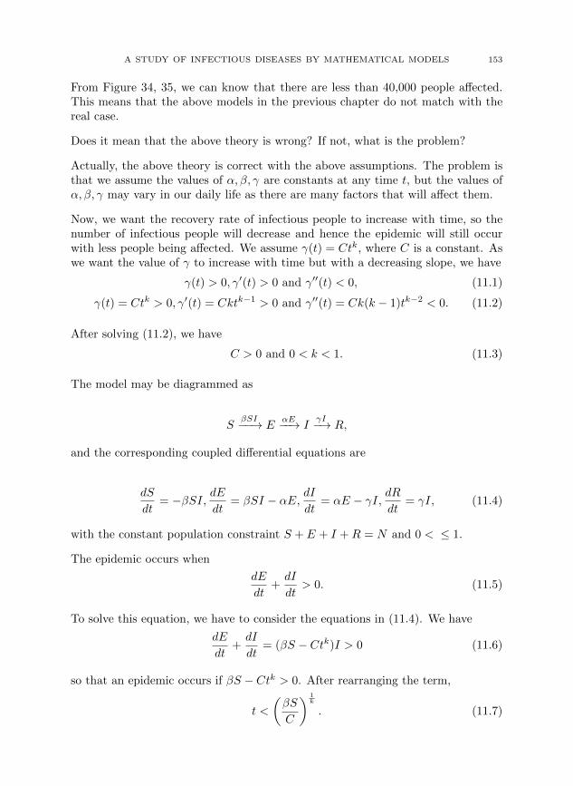
From Figure 34, 35, we can know that there are less than 40,000 people affected.This means that the above models in the previous chapter do not match with thereal case.

Does it mean that the above theory is wrong? If not, what is the problem?

Actually, the above theory is correct with the above assumptions. The problem isthat we assume the values of α, β, γ are constants at any time t, but the values ofα, β, γ may vary in our daily life as there are many factors that will affect them.

Now, we want the recovery rate of infectious people to increase with time, so thenumber of infectious people will decrease and hence the epidemic will still occurwith less people being affected. We assume γ(t) = Ctk, where C is a constant. Aswe want the value of γ to increase with time but with a decreasing slope, we have

γ(t) > 0, γ′(t) > 0 and γ′′(t) < 0, (11.1)

γ(t) = Ctk > 0, γ′(t) = Cktk−1 > 0 and γ′′(t) = Ck(k − 1)tk−2 < 0. (11.2)

After solving (11.2), we have

C > 0 and 0 < k < 1. (11.3)

The model may be diagrammed as

SβSI−−→ E

αE−−→ IγI−→ R,


dS

dt= −βSI, dE

dt= βSI − αE, dI

dt= αE − γI, dR

dt= γI, (11.4)

with the constant population constraint S + E + I +R = N and 0 < ≤ 1.


dE

dt+dI

dt> 0. (11.5)


dE

dt+dI

dt= (βS − Ctk)I > 0 (11.6)

so that an epidemic occurs if βS − Ctk > 0. After rearranging the term,

t <

(βS

C

) 1k

. (11.7)


This shows the disease will not spread out after t =

(βS

C

) 1k

. To shorten the time

of the disease spreading out, C and k should be larger. This means if there is anymedicine which can control the disease as soon as possible, the recovery rate willincrease and so the epidemic will no longer occur.

Now, we plot the graph by using the real data and numerical simulation of our

model to compare if there is any difference between them. We use γ(t) = Ct12 in

the following examples as we find that when k = 0.5, the curve will be more similarto the real case. For further study, we can try different values of k to find a moreaccurate result.

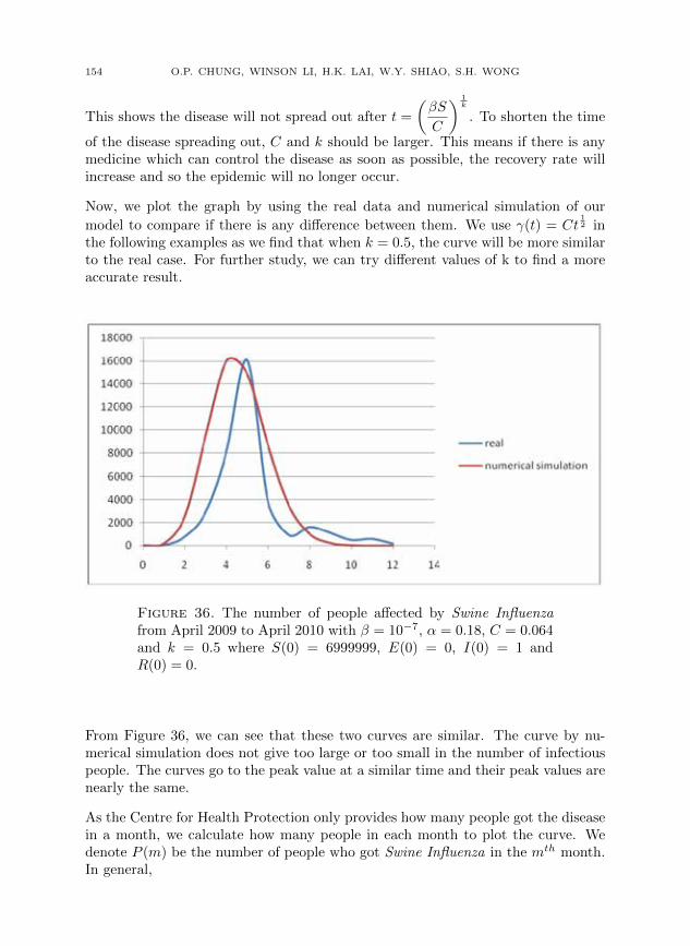
Figure 36. The number of people affected by Swine Influenzafrom April 2009 to April 2010 with β = 10−7, α = 0.18, C = 0.064and k = 0.5 where S(0) = 6999999, E(0) = 0, I(0) = 1 andR(0) = 0.

From Figure 36, we can see that these two curves are similar. The curve by nu-merical simulation does not give too large or too small in the number of infectiouspeople. The curves go to the peak value at a similar time and their peak values arenearly the same.

As the Centre for Health Protection only provides how many people got the diseasein a month, we calculate how many people in each month to plot the curve. Wedenote P (m) be the number of people who got Swine Influenza in the mth month.In general,


P (m) = S(30m− 30) + E(30m− 30)− S(30m)− E(30m) (11.8)

To derive this equation, we use the sum of the differences of the susceptible peopleand the exposed people between the beginning and the end of the month. Forexample, there are S(0) +E(0)− S(30)−E(30) people got Swine Influenza in thefirst month. By putting m = 1 to m = 12, Figure 36 was plotted.

To estimate the values of β, α,C, we can use the time of the occurrence of the secondcase of infection, the total number of people who are infected in the first monthand the time for an infectious person to recover. In the case of Swine Influenza, ittakes about a week for an infectious person to recover. Also, the number of infectedpeople in each month is known. However, we do not know the number of infectedpeople on each day and so the time of the occurrence of the second case of infectionhas to be assumed. The government departments can have a set of more accuratedata to adjust the values of β, α,C. Therefore, they can predict the number ofpeople that will be affected and when the disease is the most serious. This helpsthe government take action for a new disease.

Now, we use the case of Severe Acute Respiratory Syndrome (SARS) to see if thismodel is also similar to the case of other epidemic.

Month 03 Feb 03 Mar 03 Apr 03 May 03 Jun 03 JulNumber of

0 610 979 150 16 0people affected

Figure 37. The number of people affected by SARS in each month.

We plot the graph by using the above data and the numerical simulation to compareif there are any large differences between them and determine whether the modelsuits the real cases or not.


Figure 38. The number of people affected by SARS from Feb-ruary 2003 to July 2003 with β = 10−7, α = 0.18, C = 0.064 andk = 0.5 where S(0) = 6999999, E(0) = 0, I(0) = 1 and R(0) = 0.

From Figure 38, we can see that these two curves are also similar. Their peakvalues are similar and these curves go to the peak value at a similar time. FromFigure 36 and 38, these graphs show this model will give similar result to the realcase.

Now, we want to have some changes on γ(t) to see if there is any difference. We usethe case of Swine Influenza again. We assume γ(t) = C ln t, where C is a positiveconstant as the value of γ increases with time with the decreasing slope.


dE

dt+dI

dt> 0. (11.9)


dE

dt+dI

dt= (βS − C ln t)I > 0 (11.10)

so that an epidemic occurs if βS − C ln t > 0. After rearranging the term,

t < e

βS

C . (11.11)

This shows the disease will not spread out after t = eβSC .


Figure 39. The number of people affected by Swine Influenzafrom April 2009 to April 2010 with β = 10−7, α = 0.18, C = 0.064and k = 0.5 for the numerical simulation (γ(t) = Ctk);β =10−7, α = 0.465 and C = 0.146 for the method (γ(t) = C ln t)where S(0) = 6999999, E(0) = 0, I(0) = 1 and R(0) = 0.

Form Figure 39, we can see the curves plotted by two methods are similar to eachother. These two methods can give similar result to the real case. However, themethod by using the power of time will be better as there is one more constant kthat will affect the result and it will be easier to control the values of β, α,C. Wethink the first method, assuming γ(t) = Ctk, will be more applicable.

12. Summary

• Give an abstract, introduction of why we are studying this topic.• Have some background information about the models. Explain briefly the

modeling steps that lead to these models.• Create the simplest model - SI model, with only two basic components. Sim-

ply describe how models work.• Having the SIS SIR models as the beginning, introducing more concepts of

how we develop the models.• Developing SIVD SISR models by splitting or rearranging the existing com-

ponents.• Having the SIRS TSIR SEIR SEIRS models to show different results under

different conditions. More and more conditions are added in order to be closeto reality. Adding different conditions will change the result sharply.


• A further study in the SEIR model is made with comparison with realdata of Swine Influenza from April 2009 to April 2010 in Hong Kong, resultingin a surprising result. Find out that time is an important factor in the model.• Calculations abridged in earlier chapters are shown in Appendices.

13. Conclusion

First, we create the simplest model, the SI model. Then, by adding different newgroups, we are able to make other different and more complicated models. After aseries of investigation and research on these models, we are able to create a modelwhich gives a similar result as the real data.

Actually, in this project, we are trying to create a model which is applicable in reallife situation, aiming at predicting how the germs are spread. We try to investigatethe spreading of a disease by mathematical modeling. First, we find out the factorsaffecting the spread of diseases and possible ways to prevent epidemics. Moreover,data are put into the model to simulate the situation in Hong Kong. We are ableto find out the rate of being infected and recovery, and so as the number of peopleto be infected.

After making a number of models, and modifying them, we are able to create amodel which fits the case in Hong Kong in 2009 (Swine Influenza). We believe thatmore work can be done on these topics, aiming at the same goal, creating a modelin other situations which helps predict how germs are spread, so as to prevent them.We hope that this project can help to achieve this ultimate goal.

14. Appendices

1. Steps for solving equation (2.1)

dI

dt= βSI

dI

dt= β(N − I)I

dI

(N − I)I= βdt

∫ (1

N − I +1

I

)dI =

∫βdt

ln

∣∣∣∣I

N − I

∣∣∣∣ = Nβt+ C1

I

N − I = C2eNβt

I =NC2

C2 + e−Nβt


Put I = 1, t = 0, we have C2 =1

N − 1. Therefore,

I =N

1 + (N − 1)e−Nβtand S =

N(N − 1)e−Nβt

1 + (N − 1)e−Nβt.

2. Steps for solving equation (3.1)

dI

dt= βSI − γI (3.1)

dI

dt= β(N − I)I − γI

dI

dt+ (γ − βN)I = −βI2

(i) For <0 =βN

γ6= 1, this is in fact a Bernoulli differential equation. The

general solution is

I =

[(1− 2)

∫e(1−2)

∫(γ−βN)dt(−β)dt+ C

e(1−2)∫(γ−βN)dt

] 11−2

I =

[β

βN − γ + Ce(γ−βN)t

]−1

Since I = 1 when t = 0 and <0 =βN

γ, we have

I =

1

N

(1− 1

<0

) +

1

N

(1− 1

<0

)

e−βN

(1−

1

<0

)t

−1

(3.2)

(ii) For <0 =βN

γ= 1,

1

I2dI = −βdt,

1

I2dI = −βdt

∫ −1

I2dI =

∫βdt

1

I= βt+ C

I =1

βt+ C

Since I = 1 when t = 0, C = 1. Hence

I =1

βt+ 1(3.3)


3. Steps for solving equations (4.2)

dS

dt

=dS

dS× dS

dt× dt

dt

=1

N× (βSI)× 1

γ

=−βNγ× S

N× I

N

= −<0SI

dI

dt

=dI

dI× dI

dt× dt

dt

=1

N× (βSI − γI)× 1

γ

=βN

γ× 1

N2× SI − I

N

= <0SI − I

dR

dt

=dR

dR× dR

dt× dt

dt

=1

N× (γI)× 1

γ

= I

4. Steps for solving inequality (4.3)

<0S0 − 1 >0

<0S0 >1

βNS0

γN>1

βS0

γ>1.

5. Steps for getting (4.5)

<0(1− p) > 1

<0 − p<0 > 1

p<0 < <0 − 1

p < 1− 1

<0.

6. In chapter 11, the first case we used, i.e. assume γ(t) = Ctk, we have

S(t+ ∆t) = S(t)− βS(t)I(t)

E(t+ ∆t) = E(t) + βS(t)I(t)− αE(t)

I(t+ ∆t) = I(t) + αE(t)− γ(t)I(t)

R(t+ ∆t) = R(t) + γ(t)I(t) (13.1)

The second method we used, i.e. assume γ(t) = C ln t, we have

S(t+ ∆t) = S(t)− βS(t)I(t)

E(t+ ∆t) = E(t) + βS(t)I(t)− αE(t)

I(t+ ∆t) = I(t) + αE(t)− γ(t+ ∆t)I(t)

R(t+ ∆t) = R(t) + γ(t+ ∆t)I(t) (13.2)


There is a little bit difference between (13.1) and (13.2). It is because ifwe consider γ(0) for γ(t) = C ln t, the value of γ is undefined. So we will useγ(t+ ∆t) instead of γ(t).

REFERENCES

[1] J. R. Chasnov, Mathematical Biology,http://www.math.ust.hk/∼machas/mathematical-biology.pdf

[2] R. L. Devaney, S. Stephen and M. W. Hirsch, Differential Equations, Dynamical Systems &

An Introduction to Chaos, Elsevier Academic Press, 2004[3] H. Gaff, Ordinary Differential equations and Introduction to Dynamical Systems

http://www.tiem.utk.edu/courses/SMB02 course/dynamical.pdf

[4] M. Keeling, The Mathematics of Diseases, http://plus.maths.org/issue14/features/diseases/[5] J. Moehlis, APC/EEB/MOL 514 Tutorial 4: Seasonal Epidemic Models,

http://www.me.ucsb.edu/∼moehlis/APC514/tutorials/tutorial seasonal/tutorial seasonal.html

[6] T. Tassier, Introduction to the Modelling of Epidemics-SIS Models,http://www.facweb.iitkgp.ernet.in/∼niloy/COURSE/Spring2006/CNT/Resource/SI-

SIS.pdf


Reviewer’s Comments

The reviewer has some comments about the presentation of this paper and thetypos.

1. The reviewer has comments on the wordings, which have been amended inthis paper.

2. The reviewer suggests merging Chapter 1 into Chapter 2, because there isno additional background introduction except the formula for SI model andthere is even no definition for each variable.

3. A reference for this project may be needed.4. How about rewriting the solution of SI model as follows:

firstly, adding the two equations implies that S + I must be a constant N ,which is defined to be the population;secondly, with initial condition I(0) = 1 we can solve I and S using themethod for separable ODEs.

5. Does “we take γ−1 as time” mean “we rescale time by γ−1”?6. It may be more mathematically strict to replace “reach” with “almost reach”

or “is sufficient close to”, since the solution can only approach but never touchthe equilibrium due to uniqueness for ODE.

7. It is difficult to understand the TSIR model (8.1), especially the definitionof tourist T . There always exist self-contradictions for the following possiblecases:1) T means the total number of tourists inside Hong Kong at time t, but this

obviously contradicts with the first equation in (8.1):dT

dt= εS + εR− 2ιT ;

2) T means the total number of people who are outside Hong Kong at time tand may enter Hong Kong as tourists at an immigration rate ι, then T shouldbe a very large number, contradicting with Figure ??-??; and also it makesno sense to require S + I +R and T to be constant from the ODE system.

The reviewer suggests that:for the above case 2), set up the correct autonomous ODE system for T, S, I, R,which automatically implies T + S + I +R = constant; or else,only consider S, I,R restricted in Hong Kong but affected by the incomingtourists (at a rate 94000 per day) and outgoing ones (proportional to S+R asin the paper). This seems to better match the author’s motivation for TSIRmodel.

8. The ODE for E should bedE

dt= βSI − αE,

and the following population constraint should be S + E + I +R = N .9. The ODE for E′ should be

dE′

dt= βS′I ′ − αE′ − dE′,

and in the previous diagram, dS, dE, dI, dR should be dS′, dE′, dI ′, dR′.


10. The ODE for S,R should be

dS

dt= −βSI + µR,

dR

dt= γI − µR;

and in the previous diagram, µI from R to S should be µR;and the following population constraint should be S + E + I +R = N .

H L M A 2010 H M A Study of Infectious Diseases Through ...

Documents