gupea_2077_39774_1 copy

Bachelor’s Thesis in Financial Economics

15 ECTS

Evaluating the Efficiency of theSwedish Stock Market:

a Markovian Approach

Authors:Emil GrimsvedJohn Pavia

Supervisor:Mattias Sundén

Spring 2015Department of Economics

Evaluating the Efficiency of the SwedishStock Market: a Markovian Approach

Emil Grimsved and John Pavia∗

Abstract

This paper evaluates weak form efficiency of the Swedish stock market, by testing

whether or not the index OMXSPI follows a random walk. The returns of the index

are mapped onto one of two states, and the resulting data set is treated as a higher-

order Markov chain for the purpose of analysis. The Bayesian information criterion

is used to determine the optimal order of the chain and the null hypothesis that

the chain is of order zero is tested against the alternative that the chain is of the

established optimal order. We find that random walk behaviour cannot be rejected

for the period January 2000 to April 2015.

JEL classification: C60, G14.Keywords: efficient market hypothesis, EMH, random walk hypothesis, RWH, Markovchains, OMXSPI, time dependence, time homogeneity, weak form efficiency, Bayesianinformation criterion.

How do you beat the market? For obvious reasons this is perhaps the single mostimportant question in portfolio management. The question suggests that outperform-

ing the market is possible, which would mean that investors consistently can earn returnsthat are higher than the expected market return.

Advocates of the efficient market hypothesis (EMH) disagree. In fact, EMH directlyimplies that it is impossible to develop a trading strategy that consistently beats the

∗School of Business, Economics and Law, University of Gothenburg. We would like to thank MattiasSundén for his comments, feedback and support, which have been of great value to us. Throughout thisreport MATLAB has been used. The code and the corresponding data can be sent upon request throughmailing to [email protected].

market over time (Malkiel, 2005). This does not mean that investors cannot beat themarket, but that if they do so, it is not due to fact that they have a superior tradingstrategy; they simply owe their success to chance.

The efficient market hypothesis says that capital markets are efficient, which meansthat all available information that is relevant to the pricing of an asset is incorporatedin the price of the same asset (Fama, 1970). The concept of market efficiency is closelyrelated to the idea that the movements of stock prices are indistinguishable from thoseof a random walk. This idea is known as the random walk hypothesis (RWH). The twohypotheses are related in the sense that if stock prices indeed follow a random walk, futurestock prices cannot be predicted, and hence no trading strategy that consistently beatsthe market can be developed (Malkiel, 2005).

The opinions on the degree of efficiency in stock markets differ among financial economists,and many believe that there may be some degree of predictability in stock market returns(cf. Fama & French 1988; Malkiel, 2003; Schiller, 2014). Even so, the question of whetheror not potential patterns in returns can be exploited profitably, as well as market efficiencyas a general concept, are still highly debated topics within the field of financial economics.

Market efficiency is not just of interest as a theoretical concept; it also has implicationsfor the actions of market participants. In an efficient market all available informationabout an asset is reflected in its price, and thus market efficiency is of obvious interestsince it ensures that prices give accurate signals for investment decisions (Fama, 1970).

This paper aims to evaluate the efficiency of the Swedish stock market, by testingwhether or not the price of the index OMXSPI follows a random walk. This means thatour main interest is to test the Swedish stock market for what Fama (1970) refers toas weak form efficiency, which in turn means that the question of interest is whetheror not information about historical prices are incorporated in the current price of theindex. Many such test, for various markets, have been performed (cf. Fama, 1970, 1991,2014), including tests for the Swedish stock market (cf. Frennberg & Hansson, 1993;Shaker, 2013). The methodology has differed between the tests and for the Swedish stockmarket mostly variations of autoregressions have been the models of choice. This paperdevelops a Markovian model inspired by the one used by Fielitz and Bhargava (1973) aswell as the one used by McQueen and Thorley (1991). The model is based on the factthat independent returns is a sufficient condition for a random walk in prices, and hencerandom walk behaviour can be tested by assessing the dependence structure of returns.A data set consisting of indicator variables representing high and low returns respectivelyis constructed and tested for dependence structures by estimating transition probabilitiesunder the assumption that the data set represents a Markov chain of a given order.

The Markovian model has several advantages over an autoregressive one. It is non-parametric, and hence no assumptions about the distribution from which the data issampled have to be made. The model also allows for non-linear dependences (McQueen &Thorley, 1991), as the transition probabilities are allowed to vary depending on previously

2

realised returns. Additionally, since the returns are mapped onto states, the model isinsensitive to outliers, and therefore the whole sample can be used for the purpose ofanalysis. These advantages come at a price, as the Markovian model requires other strongassumptions; the chain representing the returns must be aperiodic, irreducible and timehomogeneous. The first two of these assumptions will be validated in the estimationprocedure, while the last one will be tested explicitly.

This paper offers an extension of previous models used to test random walk behaviourin stock market prices using Markov chains (cf. Fielitz & Bhargava, 1973; McQueen &Thorley, 1991). Instead of fixing an order of the chain, and thereby limiting the analysisto a certain dependence structure, an optimal order is derived. Further, it is shown thatpairwise tests cannot be used to reliably establish the optimal order of the chain, andtherefore an information criterion, namely Bayesian information criterion (BIC), is usedinstead. In addition, the paper contributes with a discussion on the highest testable orderof the Markov chain, and outlines the test for time homogeneity in detail. Finally, inthe test for time homogeneity a correction of the degrees of freedom of the test statisticis presented, as previous papers have either been unclear or fallacious in this particularmatter (cf. Fielitz & Bhargava, 1973; Tan & Yilmaz, 2002).

In terms of delimitations, the state space on which the Markov chain is defined onlyconsists of two states. In addition, the order of the chain is not allowed to vary over thetime period. This is mainly due to time constraints, but also due to the fact that thefocus is devoted to extending the fixed-order Markovian model to improve the reliabilityof the test. Further, only the efficiency of the Swedish stock market, represented by theindex OMXSPI, is evaluated. Data of different frequencies is, however, considered. Daily,weekly as well as monthly price data are analysed as there may be different dependencestructures in the different data sets.

To summarise, the questions this paper attempts to answer are:

• Do the prices of the Swedish stock market during the period January 2000 to April2015 follow a random walk? Equivalently, can the returns during the period bemodelled by a zero-order Markov chain?• Is the assumption of time homogeneity of the Markov chain reasonable?• Based on the results from the test for random walk behaviour, can the Swedish stock

market be considered to be weak form efficient?

The remainder of this paper is structured as follows: section I reviews previous researchon random walks and efficient markets. Section II is devoted to the efficient markethypothesis and the random walk hypothesis. In section III, which is rather technical,the methodology for testing whether or not the index OMXSPI follows a random walk isdeveloped. The data sets of interest are described in section IV. Finally, the results andthe subsequent discussion are given in sections V and VI, respectively.

3

I. A Review of Past Results

Over the last fifty years, many tests for random walks in stock prices and market efficiencyhave been published. This section presents an overview of what has been done within thefield of market efficiency and on random walks in asset prices. The overview is limited tostudies that either have used a Markovian approach or where the market of interest hasbeen the Swedish stock market.

Most studies that have tested for random walks in stock prices using a Markovianmodel have employed it on the US stock markets. For example, Niederhoffer and Osborne(1966) rejected random walk behaviour of a set of stocks traded at the New York StockExchange (NYSE) when considering intraday returns modelled by a second-order Markovchain. These results were confirmed by Fielitz and Bhargava (1973), who used a first-order Markov chain to model returns of a set of stocks. Fielitz and Bhargava includedthree states, which allowed them to model magnitudes. A random walk in stock price wasrejected for the vast majority of the stocks. In a paper from 1975, Fielitz again used aMarkov chain of order one to test for time dependence in returns of individual securitiestraded at the NYSE. For short time periods it was found that there existed a weak pricememory, which means that returns could be predicted for short time periods.

McQueen and Thorley (1991) used a second-order Markov chain to test the randomwalk hypothesis using annual returns from the NYSE. They found that the real pricesof the NYSE showed significant deviations from random walk behaviour. These resultsconfirmed findings by Lo and MacKinlay (1988). McQueen and Thorley did not test theassumption about time homogeneity of the Markov chain.

Tan and Yilmaz (2002) presented criticism against the methods that McQueen andThorley, and Fielitz and Bhargava used. The criticism was based on McQueen and Thor-ley’s failure to test if the assumptions of the model, in particular the assumption abouttime homogeneity, held. In addition, Tan and Yilmaz criticised Fielitz and Bhargava forperforming tests that required the Markov chain to be time homogeneous, even thoughthey had rejected the same assumption.

The research on market efficiency and random walks in Swedish stock prices is limited.No study has used a Markovian model to examine random walk behaviour of the Swedishstock market, but other methods such as autoregressions, variance ratio and serial cor-relation tests have been used (cf. Jennergren & Korsvold, 1974; Frennberg & Hansson,1993; Shaker, 2013).

The Swedish and Norwegian stock markets were tested for random walk behaviour byJennergren and Korsvold (1974). They considered 45 stocks, and rejected a random walkbehaviour for a majority of those. Frennberg and Hansson (1993) tested and rejectedrandom walk behaviour of the Swedish stock market for the time period 1919 to 1990.They confirmed findings from the US stock markets (cf. Lo & MacKinlay, 1988; Poterba& Summers, 1988) where returns over long periods exhibited mean reversion, while short

4

horizon returns showed positive autocorrelation. By using Swedish stock market datafrom the time period 1986 to 2004, Metghalchi, Chang and Marcucci (2008) tested threedifferent trading rules based on a moving average. They found that these trading rulescould outperform a simple buy and hold strategy even if transaction costs were included.Shaker (2013) examined the random walk behaviour of the Swedish stock market usingdaily closing prices of the index OMXS30 during the time period 2003 to 2013. He rejectedboth weak form market efficiency and random walk behaviour of the Swedish stock marketusing variance ratio and serial correlation tests.

II. Efficient Markets and the Random Walk Hypothesis

This section introduces the efficient market hypothesis and the random walk hypothesis.The section starts with a presentation of the efficient market hypothesis and discusseshow market efficiency can be evaluated. An introduction to the random walk hypothesisfollows. The section concludes with a discussion about the relationship between randomwalks in stock prices and the efficient market hypothesis.

A. The Efficient Market Hypothesis

Market efficiency has been a highly debated subject in economic theory ever since EugeneFama presented his doctoral dissertation in the 1960s. A market is said to be efficient ifall information that is available and relevant to the pricing of an asset is incorporated inthe price of the same asset (Fama, 1970, 1991). The efficient market hypothesis (EMH)then simply says that stock markets are efficient in the described sense (Fama, 1970).The term efficiency itself refers to the idea that a market with the described propertygives "accurate signals for resource allocation" (Fama, 1970, pp. 1), thus making capitalmarkets efficient.

A necessary condition for this strong version of EMH is that there are no transactioncosts, nor any expenses related to the acquiring of relevant information. Weaker versionsof the hypothesis, which have the benefit of being more economically reasonable, havebeen suggested. Jensen (1978) introduced a version where a market is efficient if themarginal benefit of acting on information is no higher than the marginal cost of the sameaction. In other words, by this definition, prices only need to reflect information on whichit would otherwise have been profitable to act.

Testing EMH is not possible unless which information set is used is specified (Fama,1970). To make the hypothesis testable Fama introduced three types of tests correspond-ing to three subsets of information (Fama, 1970, 1991): weak form tests, where the in-formation set consists of historical security prices and other market observable variables;semi-strong form tests, where the information set also includes other publicly availableinformation; and strong form tests, where private information is included as well.

5

In 1991, Fama changed these categories into ones that says more about what is actuallytested for. Weak, semi-strong and strong form tests were now introduced as tests for returnpredictability, event studies and tests for private information, respectively.

Tests of market efficiency relates observed prices to equilibrium prices in the sensethat under EMH the observed price should exhibit the properties of the equilibrium price(Fama, 2014). The efficient market hypothesis thus has to be tested jointly with an as-set pricing model, which is used to model equilibrium returns or prices. If the specifiedequilibrium asset pricing model does not hold, efficiency may be rejected because of aninadequate specification of the returns even though relevant information may be incor-porated in prices. In general there is no way of determining if market inefficiency, thepricing model or some combination of the two is the reason for the rejection (Fama, 2014).This difficulty, known as the joint hypothesis problem, makes the choosing of a reasonablepricing model a crucial part of testing EMH.

B. The Random Walk Hypothesis

The theory of random walks in stock prices dates back to 1900 when Louis Bachelierpresented his dissertation The Theory of Speculation. Fama (1965, pp. 56) defines amarket to be a random walk market if "successive price changes in individual securitiesare independent". If price changes are independent, and transaction costs are ignored,complicated trading strategies will not be more successful than a simple buy and holdstrategy, since the price development of securities cannot be predicted.

The notion that price development is unpredictable is consistent with the random walkhypothesis (RWH), which says that the movement of stock prices cannot be distinguishedfrom a those of a random walk (Fama, 1965; Malkiel, 2005). This is the same as to saythat the development of a partial sum of a sequence of independent random numbers isequally unpredictable as the future path of the asset prices. According to Fama (1965),the random walk hypothesis is not an exact description of real asset price behaviour. Evenso, the dependence structure may be weak enough to consider RWH to be a reasonableapproximate description of the movements of stock prices (Fama, 1965).

C. Random Walks and Efficient Markets

If the movements of stock prices are indistinguishable from those of a random walk in-vestors cannot possibly predict returns and hence the efficient market hypothesis is asso-ciated with the idea that stock prices follow a random walk (Malkiel, 2003). It would bemisleading to talk about any strict logical implications. The market could follow a walkbecause investors choose assets at random. While this is not likely, it illustrates that arandom walk in prices is not a sufficient condition for market efficiency. Conversely, in thecontext of this paper, as returns are divided into states one may find that one can predictthe direction of stock price movements, but not the magnitude of a rise or a fall in price.

6

Therefore, a test of RWH may lead to a situation where something can be said aboutthe behaviour of the stock market, but where it is still impossible to beat the marketconsistently.

How the efficient market hypothesis is related to the random walk hypothesis hasbeen a highly debated topic in the field of finance (cf. Lo & MacKinlay, 2002; Malkiel,2003). Lo and MacKinlay (2002) conclude that that the relationship of RWH and EMHcannot be explained in terms of sufficiency and necessity. However, economic literature(cf. Fama, 1991, 2014), suggests that a random walk in stock prices is consistent withthe efficient market hypothesis, and in many studies (cf. Fama & Blume, 1966; Jensen,1978) EMH and random walks in stock prices are evaluated in the same context. In thispaper random walk behaviour in stock prices will be considered to be an indication ofmarket efficiency and, inversely, non-random walk behaviour will be seen as evidence, butnot as proof, of market inefficiency. There will, however, be no deeper evaluation of therelationship between the two.

III. The Markovian Model

This section outlines the procedure to test for random walks in stock prices. First, theconstruction of the Markov chain1 modelled is presented. Thereafter, the Bayesian infor-mation criterion (BIC) is used to determine the order of the constructed Markov chainmodelled. The null hypothesis that the constructed chain is of order zero is then testedagainst the alternative that the chain is of the order established by BIC. This is called atest for time dependence. Finally, as the estimation of the transition probabilities requiresthat the Markov chain is time homogenous, a test for time homogeneity is given.

A. Returns and Benchmark Returns

Let Pt be the price of an asset at time t, t = 0, . . . , T . The return2, denoted rt, t ≥ 1,during the period t− 1 to t is then calculated as:

rt =Pt − Pt−1Pt−1

. (1)

Hence, rt is the percentage change from one time period to the next.The two benchmarks that are used in this paper are the geometric return and the zero

return. The geometric return is calculated as:1An introduction to the Markov theory that is used in this model can be found in appendix A.2It is worth to mention that log-returns are commonly used in empirical financial economics. One

crucial reason for this is that the logarithmic transformation make the data look more normally distributed.As the model presented in this paper does not require any normality assumption, the more direct approachof assessing returns, rather than log-returns, can be taken.

7

r =

(T∏i=1

(1 + ri)

)1/T

− 1, (2)

where T is the number of observations, i.e. the sample size of returns, and ri is calculatedas in (1). When zero is used as the benchmark r is equal to 0. In the construction of thestate space in section III.B the expected return, E[r], is replaced by r which representsthe estimate of E[r].

B. Mapping Returns to States

To model returns by a Markov chain which is discrete in both time and space, the returnshave to be divided into states. This is done by assigning a rule that maps the returns ontothe states on which the Markov chain is defined. In this paper two states are considered.Let {rt, t = 1, . . . , T} be a time series of returns. The returns are classified as "low" and"high" depending on whether or not the return is above the expected return E[r]. Let thestate space, S, consist of the two states L and H which indicate low and high returns,respectively. The returns are then mapped into this state space as follows:

Xt =

{L if rt < E[r]

H if rt ≥ E[r].(3)

Since, E[r] in (3) is unobservable it is replaced by any of the two benchmarks denoted byr.

It would be possible to consider more than two states and have each state representan interval within which the realised returns lie. The main reason for not using more thantwo states in this thesis is the difficulty of finding an unambiguous way of constructingsuch a mapping. This is, to a certain extent, true for two states as well, but at least twostates are needed for the chain to carry any information at all.

C. Estimation of Transition Probabilities

The transition probabilities of a u:th order Markov chain are estimated under the as-sumption that the chain is time homogenous. Considering a time homogenous chain, themaximum likelihood estimates of the transition probabilities are given by3:

pij =nijni.

, ∀i ∈ Su,∀j ∈ S, (4)

3A derivation of the maximum likelihood estimates of the transition probabilities can be found inappendix C.

8

which are obtained by maximising the likelihood function subject to the constraint:∑j pij = 1, i ∈ Su, j ∈ S. The counts nij and ni. denote for the number of transitions

from i ∈ Su to a specific j ∈ S and the number of transitions from i to any state j ∈ S,respectively. The observed counts are displayed in a transition count matrix (TCM). Thetransition probabilities are displayed in a transition probability matrix (TPM), and theestimated transition probabilities are displayed in an estimated TPM. Note that the esti-mation procedure requires that each row in the TCM must sum to a positive value, sinceotherwise the denominator in (4) would be zero and the expression would not even bedefined.

For a Markov chain of order two defined on the state space S = {H,L}, the TCM andthe estimated TPM are displayed in figure 1 below:

Figure 1.An illustration of the TCM and the TPM of a second-order Markov chain.The figure illustrates the transition count matrix and the estimated transition probability

matrix of a second-order Markov chain defined on a state space, S, consisting of two the statesL and H. The entries in the TCM, nLLL, . . . , nHHH are the observed number of transitions forthe second-order Markov chain followed that given path. The numbers pij are the estimated

transition probabilities for the associated sequences.

TCMPrevious Future statestates L H

L L nLLL nLLH

L H nLHL nLHH

H L nHLL nHLH

H H nHHL nHHH

TPMPrevious Future statestates L H

L L pLLL 1− pLLLL H pLHL 1− pLHL

H L pHLL 1− pHLL

H H pHHL 1− pHHL

The TCM and TPM above can be generalised to a u:th order Markov chain definedon a state space with cardinality ns in a straightforward manner.

D. Test for the Order of a Markov Chain

The aim of this section is to determine the order of the Markov chain modelled. Intuitively,multiple pairwise tests may seem appealing, and has previously been suggested by Tanand Yilmaz (2002). They presented the following procedure: the null hypothesis that theMarkov chain is of order zero is tested against the alternative that the Markov chain isof order one. If the null hypothesis is rejected, the procedure is repeated, but this timeorder one is tested against order two. The pairwise tests continue until the null hypothesisthat the Markov chain is of the lower order cannot be rejected, or until a specified highest

9

order, M , is reached. Whenever the test first fails to reject that the chain is of orderu ∈ {0, 1, . . . ,M −1}, when tested against the alternative that the chain is of order u+ 1,the chain is considered to be of order u.

However, it is possible, when testing a chain of order u + 1, that the null hypothesisthat the chain is of order u − 1, cannot be rejected when tested against the alternativethat the chain is of order u (see appendix C for further details). This shows that theprocedure suggested by Tan and Yilmaz is not reliable.

Therefore, a more reasonable approach is to use an information criterion and in thispaper the Bayesian information criterion (BIC) is used. The use of BIC when testingfor the order of the chain can intuitively be motivated by the fact that it penalises forincreasing the order of the chain if the additional information contained in the realisationsof the added periods containing the additional information is insufficient. The main reasonfor choosing BIC4, over e.g. Akaike information criterion (AIC), is that the BIC givesboth an optimal and consistent estimator of the order of the Markov chain. The use ofBIC requires that a maximum allowed order, M , is specified in advance and a method fordoing so is presented in section III.D.1. The procedure to estimate the order using BICis given in section III.D.2.

D.1. Determining the Highest Possible Order

The method used to determine the order of the chain requires that a maximum orderM is specified in advance. As it is possible, for any u ∈ N, to construct a Markov chainthat is of order u, but not of any order v ∈ N such that v < u,5 one cannot determine ahighest order without considering the nature of the data set of interest. In the contextof this paper, this would mean that one would have to present an argument for why itis economically unreasonable for a sequence of returns to be a Markov chain of an orderhigher than M .

There is, however, a technical limitation which must also be taken into consideration.For the test of the order of a chain to be valid it is required that each transition probabilityis strictly positive. This in turn implies that there must be at least one count in eachentry in the corresponding TCM. For a given chain this means that once the order is highenough for the corresponding TCM to have an entry which equals zero, one must assumethat the chain is not of this or any higher order.

In this paper the maximum order,M , will be set to the highest order that correspondsto a TCM whose entries are all non-zero. The motivation for choosing the maximum orderM this way is simple. As it is a stronger assumption that a chain is of order u ∈ N thanthat the chain is of order u+ 1, and hence the largerM is, the weaker the assumption onehas to make about the order of the chain becomes. By choosing M as above it gives the

4The Bayesian information Criterion is also known as Schwartz Bayesian criterion (SBC) since it wasfirst derived by Schwartz (1978) to find the optimal dimension for the model used.

5In appendix C an example of such a construction is shown.

10

largest possible maximum order and hence also the weakest possible assumption aboutthe order of the chain for each data set.

D.2. Test for the Order by Using an Information Criterion

This section describes a method, first presented by Anderson and Goodman in 1957,for deciding whether or not the TPM of a Markov chain of order v < u is statisticallydifferent from the TPM of a chain of order u. The method is required to determine anorder using the Bayesian information criterion (BIC). The order established using BICis optimal, in the specific sense that, under the assumptions that the prior distributionis a non-informative Dirichlet distribution, it minimises the expected loss (Katz, 1981).The established order does not depend on either the prior distribution or the posteriordistribution (Katz, 1981).

The BIC procedure requires that the state space, S, is finite and that the Markovchain is aperiodic and irreducible. Furthermore, as stated above, a maximum order, M ,has to be specified. By determining M as above the assumptions of irreducibility andaperiodicity are fulfilled. Further, the state space S = {L,H} is finite. Hence, theassumptions hold.

As for the testing procedure, which is based on the work of Anderson and Goodman(1957), consider a sequence of data which may be represented by a Markov chain. Theobjective is to test if the Markov chain is of order v against the alternative that the Markovchain is of order u. It can be assumed, without loss of generality, that v < u. In this settingthere are three sequences to consider; u = in−u, . . . , in−1 ∈ Su which carries informationin the Markov chain of order u; v = in−v, . . . , in−1 ∈ Sv, which carries information in theMarkov chain of order v; and d = in−u, . . . , in−(v+1) ∈ Sd = Su−v, which belongs to theset of sequences that separate the sequences in Su from the ones in Sv, it follows thatu = dv. The transition probabilities using this newly introduced notation for the chain oforder u and the chain of order v are defined in equations (5) and (6), respectively:

puj = P(Xn = j|Xn−1 = in−1, . . . , Xn−v = in−v, . . . Xn−u = in−u) = pdvj , (5)

pvj = P(Xn = j|Xn−1 = in−1, . . . , Xn−v = in−v). (6)

Let nuj = ndvj be defined as the number of transitions following the sample pathin−u . . . in−v . . . in−1j for the Markov chain of order u. Analogously nvj is defined asthe number of transitions following the path in−v . . . in−1j for the v:th order chain. De-fine nu. = ndv. and nv. as the total number of transitions following the sample pathsin−u . . . in−v . . . in−1 and in−v . . . in−1 for the Markov chains of order u and v, respectively.

11

Then the maximum likelihood estimates of the transition probabilities are calculated asin (4). However, using the notation introduced above, the transition probability given in(4) is now given by (7) and (8) for the chains of order u and v, respectively:

puj =nujnu.

=ndvjndv.

= pdvj , (7)

pvj =nvjnv.

. (8)

The null hypothesis, H0, and the alternative hypothesis, H1, can be formulated6 asbelow:

H0 : the chain is of the lower order v,H1 : the chain is of the higher order u, but not of the lower order v.

The likelihood ratio statistic Λv for a given sequence, vj, is given below:

Λv =∏v,j

(pvjpdvj

)ndvj

. (9)

There are nu−vs unique sequences in which the sample paths coincide. Therefore, the teststatistic Λ becomes the product of the test statistics Λv. This is to say that:

Λ =∏d

Λv =∏d

∏v,j

(pvjpdvj

)ndvj

=∏d,v,j

(pvjpdvj

)ndvj

. (10)

Taking the transform −2 log(Λ), the limiting result becomes:

− 2 log(Λ) = 2∑d,v,j

ndvj log

(pdvjpvj

)a∼ χ2

df , df = (nus − nvs)(ns − 1). (11)

The test statistic −2 log(Λ) under the null hypothesis is asymptotically Chi-squared dis-tributed with (nus − nvs)(ns − 1) degrees of freedom. Which is a generalisation of the teststatistic derived in Anderson and Goodman (1957).

6The aim is to test whether or not the probability distribution of the u:th and v:th order Markovchains are the same. Mathematically, the null and alternative hypotheses can be stated as:

H0 : ∀u ∈ Su, ∀j ∈ S; puj = pvjH1 : ∃u ∈ Su, ∃j ∈ S; puj 6= pvj .

12

Under the assumptions that the Markov chain is aperiodic, irreducible and defined ona finite state space S, with an upper boundM of the order of the chain, the BIC estimatorfor the order of the chain is defined below.

DEFINITION 1: Let X be a Markov chain of order u < M . Let the likelihood ratio statis-tic, Λ, for testing order u versus order M be denoted by Λu,M , then the BIC estimator,uBIC, for the order of the Markov chain is such that:

f(uBIC) = min0≤u<M

f(u), (12)

where f(u) = −2 log(Λu,M )− (nMs − nus )(ns − 1) log(T ), T is the sample size and(nMs − nus )(ns − 1) is the degrees of freedom for the likelihood ratio statistic Λu,M .

The likelihood ratio test statistic is at least as large when an order higher than u istested against v, as it is when testing u against v. In the same sense as adding explanatoryvariables to a linear regression model never reduces the fit, adding periods that may carryinformation in the Markov chain never reduces the likelihood ratio statistic. Therefore, inthe testing procedure the term (nMs −nus )(ns−1) log(T ) penalises for increasing the order,which can be compared to utilising the adjusted R-squared when additional explanatoryvariables are added to a multiple linear regression.

It should be noted that, when using BIC for estimating the order of a Markov chain,one tests the highest allowed orderM against all lower orders 0, 1, . . . ,M−1 (Katz, 1981).If BIC gives the optimal order 0, then the BIC only says that this order best represents thedata when penalising for the increased order. It does not determine whether or not thereis any dependence structure in the returns. Thus, to be able to perform a significancetest for time dependence, the optimal order, determined using BIC, must be at least1. Therefore, we have chosen to test the maximum order M against the lower ordersu ∈ {1, . . . ,M − 1}.

E. Testing if the Order of the Chain is Different from Zero

Assuming that an optimal order u has been established using BIC, u is the optimal order(or, rather, the optimal order different from zero) of the Markov chain, but BIC saysnothing about whether or not this order results in a plausible model. If every order of thechain results in a bad model, BIC just gives us the least bad of these models. Therefore,a test must performed to determine whether the order established using BIC results in amodel that is significantly better than a Markov chain of order zero.

Under the assumption of time homogeneity, the null and alternative hypotheses can

13

be stated7 as below:

H0 : The chain of the optimal order is also a chain of order 0,H1 : the chain of the optimal order is not a chain order 0.

The point estimate, p.j , of p.j , j ∈ S is under the null hypothesis, given by:

p.j =n.jn.., (13)

where n.j is the sum of transitions to state j for all prior sequences i ∈ Su and n.. is thetotal number of transitions to any state for all prior sequences, which is the same as thesample size.

The test statistic for testing the null hypothesis, H0, against the alternative hypothesis,H1, is given by equation (11) where the v:th order is zero and the u:th order is the optimalorder established using BIC. The test statistic under the null hypothesis is asymptoticallyChi-square distributed with (nus − 1)(ns − 1) degrees of freedom.

F. Testing for Time Homogeneity of a Markov Chain

The transition probabilities of the Markov chain is estimated under the assumption oftime homogeneity. This assumption has to be validated. A quite intuitive procedure,based on the work of Anderson and Goodman (1957), for testing time homogeneity is todivide the time series into N > 1 subintervals of equal length. For time homogeneity to bevalid, the TPM must be the same for each of the N subintervals of time. Let subintervalk be denoted by Ik, k = 1, . . . , N . Given that the Markov chain of order u has taken thepath i ∈ Su in subinterval Ik, the transition probability of moving to j ∈ S is denoted asfollows:

pkij = P(Xn = j|Xn−1 = in−1, . . . , Xn−u = in−u), n ∈ Ik, i ∈ Su, j ∈ S. (14)

The transition probabilities of each subperiod of time are estimated completely analo-gously to the transition probabilities over the whole time period, using (4) for the subpe-riods sample. The aim is to test whether or not the TPM for each subperiod is the same

7The aim is to test whether or not the probability distribution is the same for the optimal order andthe zero-order chains. Let p.j denote the probability of moving to state j ∈ S regardless of the priorsequence. Mathematically, the null and alternative hypotheses can be described as:

H0 : ∀i ∈ Su, ∀j ∈ S; pij = p.jH1 : ∃i ∈ Su, ∃j ∈ S; pij 6= p.j .

14

as the TPM for the whole period. The null and alternative hypotheses can be expressed8

as:

H0 : the Markov chain is time homogenous,H1 : the Markov chain is time heterogeneous.

Under the null hypothesis the likelihood ratio test statistic, Λ, becomes:

Λ =

N∏k=1

∏i∈Su,j∈S

(pij

pkij

)nkij

. (15)

The likelihood ratio test statistic, Λ, is asymptotically equivalent to:

−2 log(Λ) = 2N∑k=1

∑i∈Su,j∈S

nkij log

(pkijpij

). (16)

The test statistic −2 log(Λ), under H0, is asymptotically Chi-squared distributed with(N − 1)nus (ns − 1) degrees of freedom9. Here pkij is the estimate of (14) and pij is theestimate of the transition probability of the u:th order Markov chain over the whole timeperiod, which is given by (4). Since all subintervals are compared to the whole time periodthe problem of multiple comparisons becomes apparent. Bonferroni’s method, by whichthe significance level is adjusted based on the number of comparisons made, is used.

IV. Data

In this section the data used in this paper is presented and described in detail. Ad-ditionally, some summary statistics of the data are given. The data used in this pa-per is the Nasdaq OMXSPI index, also known as the Stockholm all share index. Thisindex represents the value of all shares that are traded at Stockholm stock exchange(http://www.nasdaqomxnordic.com). The price data consists of the closing prices of theindex OMXSPI for days, weeks and months respectively (non-trading days are excluded).10

The index OMSXPI is used as a proxy for the Swedish stock market. The motivation8Let the TPM for the k:th subinterval be denoted by Pk and the TPM for the whole time period be

denoted by P. The objective is to test whether or not the transition probabilities from each subperiod isthe same as the transition probabilities for the whole time period. The null hypothesis and the alternativehypothesis can then mathematically be stated as:

H0 : ∀k ∈ {1, . . . , N};Pk = P

H1 : ∃k ∈ {1, . . . , N};Pk 6= P.

9In appendix C a motivation for this number of degrees of freedom can be found.10The data used has been downloaded 2015-04-25 through the Bloomberg terminal.

15

for using this index over the index OMXS30 is that it includes all traded stocks at theStockholm Stock Exchange while OMXS30 only consists of the 30 most traded stocks.Therefore, the index OMXSPI serves better as a proxy for the Swedish stock market as awhole than OMXS30 does.

The time period used in this study is January 2000 to April 2015. In particular, for thedaily price data, the statistics are based on observations from the time period 2000-01-02to 2015-04-23. The weekly prices come from the period 2000-01-07 to 2015-04-17 and forthe monthly closing prices the period 2000-01-31 to 2015-03-31 has been considered. Thereturns are calculated as in (1). In table I some descriptive statistics of the samples usedthroughout this paper are shown11.

Table IDescriptive Statistics of Prices and Returns.

The table shows some descriptive statistics of daily, weekly and monthly closing prices and thecorresponding returns of the index OMXSPI during the period January 2000 - April 2015. Inthe left part of the table the descriptive statistics of the prices are shown and in the right partthe corresponding descriptive statistics of the returns are shown. The statistics shown are themean, median, standard deviation (Std.), the minimum and maximum value, the inner quantile

range (IQR), the skewness, kurtosis and the number of observations (No. obs.).

Descriptive statistics of prices.The descriptive statistics of closing prices

during the period January 2000 - April 2015.

Daily Weekly Monthly

Mean 302.5067 302.5237 302.6447Median 307.3150 306.8850 308.4100Std. 86.2225 86.3420 86.7245Min 126.4100 134.3700 134.3700Max 560.5500 556.1700 548.6400IQR 129.3800 128.3900 130.4650Skewness 0.1800 0.1721 0.1637Kurtosis 2.6567 2.6238 2.6365No. obs. 3842 798 183

Descriptive statistics of returns.The descriptive statistics of returns during the period

January 2000 - April 2015.

Daily Weekly Monthly

Mean 0.0002 0.0011 0.0043Median 0.0007 0.0040 0.0066Std. 0.0144 0.0298 0.0568Min -0.0775 -0.2059 -0.1789Max 0.0901 0.1161 0.1873IQR 0.0144 0.0315 0.0568Skewness 0.0793 -0.6785 -0.2641Kurtosis 6.5072 7.0059 4.1830No. obs. 3841 797 182

V. Test Results

This section presents the results from the various tests we have performed on the Markovchain constructed from the returns of the index OMXSPI. All of these tests are discussedin greater depth in section III, where the Markovian model used in this paper is presented.

11In appendix B plots of time series of prices and returns for the index OMXSPI during January 2000to April 2015 are given for daily, weekly as well as monthly data.

16

It is found that the optimal order of the Markov chains representing daily, weekly andmonthly returns is 1. This is true both when the benchmark is the geometric return andwhen it is the zero return. Further, it is found that a random walk behaviour of theSwedish stock market cannot be rejected, nor can the assumption of time homogeneity berejected, for any of the benchmarks and for all frequencies of returns.

A. The Optimal Order

The highest order allowed for the chain is determined as described in section III.D.1 foreach of the frequencies. The highest order allowed is denoted by M in table II. Note thatM does not need to be the same for all frequencies of returns. The statistic −2 log(Λu,M )

(see definition 1) is denoted by ηu,M to simplify the notation in table II. Further, f(u)|Mdenotes the BIC statistic, where order u is tested against order M . In table II these twostatistics are displayed for daily, weekly and monthly returns of OMXSPI.

17

Table IITest results for the test of the order.

The table shows the test results for the optimal order of the Markov chains, as determined byBIC, describing daily, weekly and monthly returns of the index OMXSPI during the period

January 2000 - April 2015. In the first part of the table the benchmark return is the geometricreturn and in the second part of the table the benchmark is the zero return. The variable f(u)|Mdenotes the test statistic calculated using the Bayesian information criterion and the variableηu,M is the test statistic calculated in the test of order u against the highest order allowed M .

Geometric return.The benchmark return used to construct the Markov chain is the geometric return.

Daily Weekly Monthly Daily Weekly Monthlyu f(u)|M=7 f(u)|M=5 f(u)|M=3 ηu,M=7 ηu,M=5 ηu,M=3

1 -915.3 -175.7 -18.2 124.4 24.5 13.02 -902.0 -163.2 -9.7 121.2 23.7 11.03 -870.6 -137.4 - 119.6 22.8 -4 -811.1 -94.4 - 113.0 22.8 -5 -692.6 - - 99.5 - -6 -470.9 - - 57.2 - -

Zero return.The benchmark return used to construct the Markov chain is the zero return.

Daily Weekly Monthly Daily Weekly Monthlyu f(u)|M=7 f(u)|M=5 f(u)|M=3 ηu,M=7 ηu,M=5 ηu,M=3

1 -914.5 -175.9 -19.3 125.2 24.3 11.92 -900.4 -163.0 -11.2 122.9 24.0 9.63 -868.8 -137.6 - 121.4 22.6 -4 -807.2 -95.7 - 117.0 11.1 -5 -686.3 - - 105.9 - -6 -470.0 - - 58.2 - -

From table II one can see that the function value f(u)|M is the smallest for u = 1 forall the three frequencies of returns for both the benchmarks. Hence, the optimal order ofthe Markov chain representing daily, weekly and monthly returns is 1. This is true forboth benchmarks used to construct the Markov chain modelled.

B. Time Dependence in Returns

With the optimal order established, the test for time dependence is, as described in sectionIII.E, simply a matter of testing a chain of the established optimal order against a chain of

18

order 0. In this case, the optimal estimate of the order, i.e. the BIC estimate of the order,is 1 for all the three frequencies of returns. This means, for daily, weekly and monthlyreturns, that the null hypothesis that the Markov chain is of order 0 is tested against thealternative hypothesis that it is of order 1, for each of the frequencies of returns and bothbenchmarks.

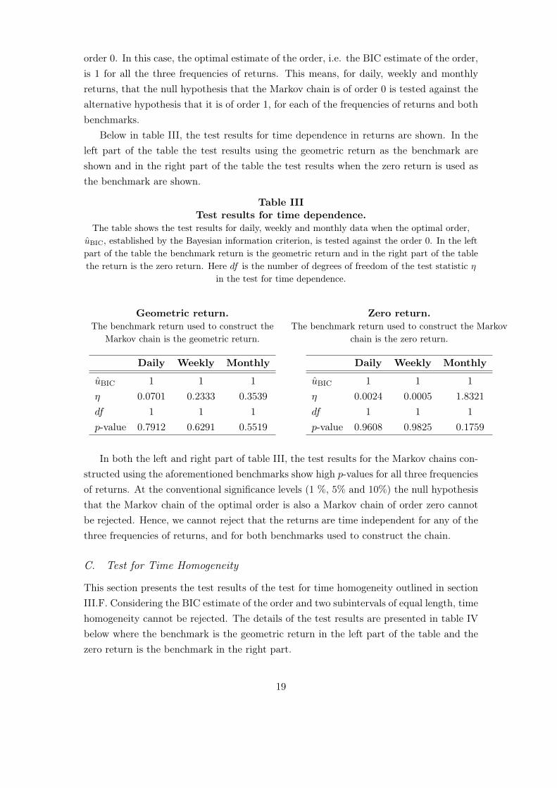
Below in table III, the test results for time dependence in returns are shown. In theleft part of the table the test results using the geometric return as the benchmark areshown and in the right part of the table the test results when the zero return is used asthe benchmark are shown.

Table IIITest results for time dependence.

The table shows the test results for daily, weekly and monthly data when the optimal order,uBIC, established by the Bayesian information criterion, is tested against the order 0. In the leftpart of the table the benchmark return is the geometric return and in the right part of the tablethe return is the zero return. Here df is the number of degrees of freedom of the test statistic η

in the test for time dependence.

Geometric return.The benchmark return used to construct the

Markov chain is the geometric return.

Daily Weekly Monthly

uBIC 1 1 1η 0.0701 0.2333 0.3539df 1 1 1p-value 0.7912 0.6291 0.5519

Zero return.The benchmark return used to construct the Markov

chain is the zero return.

Daily Weekly Monthly

uBIC 1 1 1η 0.0024 0.0005 1.8321df 1 1 1p-value 0.9608 0.9825 0.1759

In both the left and right part of table III, the test results for the Markov chains con-structed using the aforementioned benchmarks show high p-values for all three frequenciesof returns. At the conventional significance levels (1 %, 5% and 10%) the null hypothesisthat the Markov chain of the optimal order is also a Markov chain of order zero cannotbe rejected. Hence, we cannot reject that the returns are time independent for any of thethree frequencies of returns, and for both benchmarks used to construct the chain.

C. Test for Time Homogeneity

This section presents the test results of the test for time homogeneity outlined in sectionIII.F. Considering the BIC estimate of the order and two subintervals of equal length, timehomogeneity cannot be rejected. The details of the test results are presented in table IVbelow where the benchmark is the geometric return in the left part of the table and thezero return is the benchmark in the right part.

19

Table IVTest results for time homogeneity of the chain of the optimal order.

The table shows the test results for time homogeneity of the Markov chains of the optimal order,uBIC, representing daily, weekly and monthly returns of the index OMXSPI during the timeperiod January 2000 - April 2015, when the time series of returns is divided into N = 2

subintervals of equal length. The test statistic of the test for time homogeneity is denoted byηuBIC,N . In the left part of the table the benchmark used to construct the chain is the geometric

return and in the right table the benchmark is the zero return.

Geometric return.The benchmark return used to construct the

Markov chain is the geometric return.

Daily Weekly Monthly

uBIC 1 1 1N 2 2 2ηuBIC,N 3.7140 2.6171 1.3805df 2 2 2p-value 0.1561 0.2702 0.5115

Zero return.The benchmark return used to construct the

Markov chain is the zero return.

Daily Weekly Monthly

uBIC 1 1 1N 2 2 2ηuBIC,N 3.8915 2.0733 1.3455df 2 2 2p-value 0.1429 0.3546 0.5103

Here ηuBIC,N denotes for the test statistic in (16), where uBIC is the optimal orderestablished using BIC and N is the number of subintervals of equal length the data setis divided into to perform the test for time homogeneity. For the estimation procedureoutlined in section III.C to be valid the chain has to be homogenous. The high p-valuesshow that time homogeneity cannot be rejected for the optimal order for any of the chainsrepresenting daily, weekly and monthly returns of OMXSPI if the conventional significancelevels are considered. This is true both when the geometric return and the zero returnare used as benchmarks.

In table V below, the test results for time homogeneity of the Markov chain of order0 are shown. In the left part of the table, the test results when the geometric return isused as the benchmark are shown and the test results when the zero return is used as thebenchmark are shown in the right part.

20

Table VTest results for time homogeneity of the chain of order zero.

The table shows the test results for time homogeneity of the Markov chains of order 0representing daily, weekly and monthly returns of the index OMXSPI during the period January2000 - April 2015 when the time series of returns is divided into N = 2 subintervals of equal

length. The test statistic of the test for time homogeneity is denoted by ηuBIC,N . In the left partof the table the benchmark used to construct the chain is the geometric return and in the right

part of the table the benchmark is the zero return.

Geometric return.The benchmark return used to construct the

Markov chain is the geometric return.

Daily Weekly Monthly

u 0 0 0N 2 2 2η0,N 0.2671 0.3054 0.8571df 1 1 1p-value 0.6053 0.5805 0.3546

Zero return.The benchmark return used to construct the

Markov chain is the zero return.

Daily Weekly Monthly

u 0 0 0N 2 2 2η0,N 0.1388 0.2731 3.6785df 1 1 1p-value 0.7094 0.6013 0.0551

The p-values corresponding to daily, weekly and monthly returns, in table V are wellabove any conventional significance level when the geometric return is used as the bench-mark. Hence, time homogeneity cannot be rejected for the chains representing the afore-mentioned frequencies, when the geometric return is used as benchmark. When the zeroreturn is used as the benchmark, time homogeneity cannot be rejected for the Markovchains of order 0 representing daily and weekly returns. The p-value for the Markov chainrepresenting the monthly returns is slightly above 5 %. However, in this case a significancelevel of 5 % corresponds to an overall significance level of 10 % when Bonferroni’s methodis used, since two comparisons are made when there are two subintervals. This meansthat time homogeneity cannot be rejected at the 10 % significance level for any of thethree frequencies of returns.

VI. Discussion

The research on market efficiency and random walks in stock prices is as various as it isvoluminous. This section aims to place the method developed and the tests performed inthis paper in a larger context. It also discusses the reliability of the model used, as wellas how the joint hypothesis problem appears in this setting.

The section starts with a brief summary of the results and the conclusions that canbe drawn from these, and a validation of the of the assumptions about the Markov chainmodelled follows. Thereafter, the joint hypothesis problem is addressed in conjunction

21

with a discussion on the choosing of benchmarks. The section continues with a comparisonwith previous research in which random walks in asset prices and weak form efficiency ofthe Swedish stock market have been evaluated, and thereafter a comparison with studiesin which a Markovian approach has been used to test for random walk behaviour in stockprices is made. In particular, the difference in methodology is discussed. A discussionabout what this paper brings to the research on market efficiency and random walks instock prices in general, and to research using a Markovian approach in particular, follows.The section ends with possible extensions of the presented model that have not beenimplemented within the frame of this paper, but may be of interest for further research.

A. Summary

We find that the random walk hypothesis cannot be rejected for the index OMXSPI forthe period January 2000 to April 2015, using the Markovian methodology presented anddeveloped in this paper. This holds true for daily, weekly as well as monthly returns.Further, time homogeneity cannot be rejected for any of the data sets of returns. Noevidence that supports that prices can be predicted using historical data is found, whichis consistent with that the Stockholm Stock Exchange is weak form efficient.

B. Validation of the Assumptions

The method presented in section III requires the Markov chain representing the stockreturns to be aperiodic, irreducible and time homogeneous. If the analysis concerningrandom walks and efficient markets is to carry any weight, these assumptions need to bevalidated.

Aperiodicity and irreducibility of the estimated chains are implicitly tested for both inthe use of BIC and in the test for time homogeneity, as computations of the test statisticsrequire that the transition probabilities are strictly positive. This is a sufficient conditionfor aperiodicity and irreducibility of the chain.12

Time homogeneity is explicitly tested for, and cannot be rejected for any of the datasets considered in this paper. This increases the reliability of the results as time homo-geneity is a necessary condition for the estimation of the TPMs to be valid. However, itshould be noted that a failure to reject time homogeneity is not the same as acceptingthat the chain is time homogeneous; it simply means that, when dividing the chain into anumber of subintervals of equal length, the transition probabilities of the subintervals are

12It is easy to see that the chain is aperiodic, since whenever all transition probabilities in the TPMare strictly positive each possible path ij, i ∈ Su, j ∈ S can be taken by the chain. As all entries in theTPM are positive, it is possible to move from any previous path i ∈ Su to any state j ∈ S, this includesany path that ends with j (i.e. the state which the chain moves to). Therefore it is possible to movefrom a given state to the same state in one step; hence the period of every state is one and the chain isaperiodic. Also, as all entries are positive it is possible to move to any state from any other state, whichmeans that the chain is irreducible.

22

not significantly different from the transition probabilities over the whole period. Nev-ertheless, the failure to reject the null hypothesis does support the assumption of timehomogeneity, in the sense that if there would have been a large difference between theTPMs of the different subintervals and the TPM over the entire period, time homogeneitywould have been rejected.

C. The Joint Hypothesis Problem and the Choosing of Benchmarks

The joint hypothesis problem, discussed in further detail in section II.A, states that theefficient market hypothesis must be tested jointly with an equilibrium pricing model.This means that to decide whether or not any excess returns can be made, one mustfirst establish a level of returns which can be considered "normal". In this paper, abenchmark return is used to represent the normal return and the simple mapping rule isthat any return above the benchmark is classified as "high", and any return below thesame benchmark is classified as "low". The benchmarks used to determine in which stateto place the return over one time period is the zero return and the geometric return,respectively.

The use of zero as a benchmark is motivated by the fact that any positive returnincreases the value of a portfolio. Abstracting from reality and considering a risk-freereturn of zero, investors would prefer to keep their money in the market during such aperiod. Inversely, a negative return would mean that investors would prefer to stay outof the market. In this setting, it does not matter whether zero is considered to be high orlow, as if the return is zero over a period, any investor would be indifferent as to wheretheir money is placed.

A return of zero cannot be said to equal the expected return, as empirical evidencesuggests that the expected return of the market should be positive for long time periods.Because the mapping fails to account for magnitudes, it is also impossible to say whichperiods are the most profitable, or even if a period is more profitable than the average one;all that can be concluded is that the return is positive. Because of this, the benchmarkzero is not to be seen as an equilibrium return in an empirical setting, but as a possibleequilibrium return in a theoretical abstraction, which can be used to investigate patternsin historical prices.

The other benchmark return that is used is the geometric return, which can hardly bedescribed as the expected return at any time during the time period. Even if the futurewould be like the past in a probabilistic sense, which would let the geometric return upto a given time point act as a benchmark return for the same point in time, there is noreasonable argument for the opposite. Hence, the geometric return is not to be treatedas an equilibrium return, but rather as a benchmark against which the performance of anindividual stock can be measured. So, while it cannot be said about returns above thegeometric return that they have beaten some kind of expectation, it can be said that they

23

have performed well relatively to an unbiased average.

D. Comparisons With Other Studies

This section compares our results to previous studies, which are divided into two cate-gories. First, our results are compared to other studies that focused either exclusively orpartly on random walk behaviour of the Swedish stock market and Swedish stock mar-ket efficiency. Thereafter, a comparison with other studies which have used a Markovianapproach is made.

D.1. Comparisons With Other Tests for Swedish Stock Market Efficiency

In section I, four studies that tested the Swedish stock market for random walk behaviourin stock prices and weak form efficiency are discussed. Three of these studies concernedrandom walks in stock prices (Jennergren & Korsvold, 1974; Frennberg & Hansson, 1993;Shaker, 2013). The exception is the study by Metghalchi, Chang and Marcucci (2008),which tested for the profitability of three trading rules based on moving averages.

Metghalchi, Chang and Marcucci (2008) found that trading rules based on movingaverages can be profitable even when transaction costs are accounted for, which violatesboth weak form market efficiency and that stock prices follow a random walk. Theseresults stand in contrast to the results obtained using the Markovian approach in ourpaper, which suggest that a random walk behaviour of the Swedish stock market cannotbe rejected. One possible explanation for the difference in results is that the time periodused differs. As mentioned in section I Metghalchi, Chang and Marcucci used data fromthe period 1986 to 2004. As of today, when the computer technology is developed to alarge extent, such profit opportunities are more likely to vanish rapidly, as high-frequencyrobots exploit such opportunities instantly.

In contrast to our results studies by Jennergren and Korsvold (1974) as well asFrennberg and Hansson (1993) reject random walks in stock prices of stocks traded atthe Swedish stock market. The difference in results can be explained by several factors.The time series used is not the same since our sample is from the 21st century while theirsamples are from the 20th century. It is possible that the market was less random prior tothe development of fast computer communications. Furthermore, the methodology usedin this paper differs from the ones used in these two papers. In addition, Jennergren andKorsvold did use individual stocks traded at the Swedish stock exchange while we use anindex as a proxy for the Swedish stock market.

A comparison to Shaker (2013) is especially appealing since Shaker uses the indexOMXS30 from January 2003 to January 2013 which is very similar to OMXSPI for theperiod January 2000 to April 2015, which is used in this paper. Shaker rejected randomwalk behaviour for this time period while we conclude that a random walk in the price ofthe index OMXSPI cannot be rejected. The Markovian model that is used in the context of

24

this paper differs from the linear model Shaker used to test for serial correlation in returns.Since these two indices are very similar and the time period Shaker used is included in oursample’s time period the difference in results is surprising. One possible explanation couldbe that some assumptions in either our Markovian model or in Shakers linear model havebeen violated. However, none of the assumptions made in the Markovian model in thispaper can be rejected. Another possible explanation can be the choosing of benchmarkin the construction of the Markov chain. Other benchmarks, which are not considered inthis paper, might give different results.

D.2. Comparisons With other Markovian Studies

There are other papers that have used Markovian models for testing random walk be-haviour in stock prices, e.g. those presented in section I (cf. Niederhoffer & Osborne,1966; Fielitz & Bhargava, 1973; Fielitz, 1975; McQueen & Thorley, 1991; Tan & Yil-maz, 2002). This section goes through some of the important differences of our paper ascompared to earlier papers that have used Markovian models.

The main difference between the Markovian model in this paper and the Markovianmodels in earlier papers is how the order is established. McQueen and Thorley (1991),Fielitz and Bhargava (1973), and Fielitz (1975) chose a model with a specified order,they did not test if this order was optimal or not. Nevertheless, it should be mentionedthat McQueen and Thorley presented some arguments supporting their choice to use asecond-order markovian model. Our model on the other hand, does not make any a prioriassumption regarding the order of the chain, instead an optimal order is derived. Tan andYilmaz (2002) did address how to determine which order to use. However, the procedurethey suggested for determining the order is incorrect. Since every Markov chain of orderu is a chain of order u+ 1 as well, it is not possible to make the pairwise tests of orders asthey suggested. In our paper BIC is used to get around this problem. Both the consistencyand the optimality of the BIC estimator give additional support for the usage of BIC.

Further, some papers that have used a Markovian model for testing random walkbehaviour in stock prices have made crucial assumptions that were never tested for. Mc-Queen and Thorley (1991) assumed time homogeneity of the Markov chain representingthe returns of the NYSE, without testing for it. Fielitz and Bhargava (1973) on the otherhand were aware of the importance of time homogeneity. They tested for it, rejected it,and still proceeded with the analysis and rejected random walk behaviour of the stocksconsidered. The assumption of time homogeneity is tested and cannot be rejected forthe samples considered in this paper, which is the best possible outcome since the nullhypothesis is must be that the chain is time homogenous.

Tan and Yilmaz (2002) criticised McQueen and Thorley (1991) for not testing theassumption of time homogeneity. According to Tan and Yilmaz the assumption of timehomogeneity would have been rejected for the data set McQueen and Thorley (1991)

25

used. Nonetheless, the null distribution of the test statistic Tan and Yilmaz suggestedhad the wrong degrees of freedom (see appendix C for the correct degrees of freedom).This paper uses an approach first suggested by Anderson and Goodman (1957) for testingthe assumption of time homogeneity, which is similar to the approach used by Fielitzand Bhargava (1973), and Fielitz (1975). However, our results can be reproduced as thenumber of subintervals used is stated explicitly, which is not the case in the papers byFielitz and Bhargava, and Fielitz.

E. Contributions

This paper offers an alternative approach for testing for a random walks in stock pricesusing a Markovian model to capture dependence structures in returns, which may benon-linear. One big advantage of this model compared to others, is that the model isnonparametric, i.e. no assumptions about the distribution of returns have to be made.The main contribution to the field of market efficiency and random walk theory is thedevelopment of an existing method for testing for random walk behaviour of a stockmarket, in the sense that this paper provides a way to optimally determine the order ofthe Markov chain modelled. Furthermore, it does contribute with a crucial correction ofthe asymptotic distribution of the test statistic used in the test for time homogeneity inearlier studies. From an economic point of view, this paper contributes with test resultson random walk behaviour in prices, using a method which, as far we know, never hasbeen applied to the Swedish stock market.

F. Suggestions for Further Studies

One of the restrictions within the scope of this paper is that the state space consists of onlytwo states. Future studies may use the method presented in this paper, but include morestates, which would allow the model to capture not only the directions, but also, to somedegree, the magnitudes of the returns. Another suggestion would be to use two states,one state that represents positive returns and one that represents negative returns, and inaddition to these states include a variable that predicts the magnitude of a return, giventhat it is positive, or negative, and has followed a particular path. Such a model has beenused by Lennartsson, Baxevani and Chen (2008) to capture the amount of precipitationin Sweden.

The model can be extended to a vector process (cf. Fielitz & Bhargava, 1973), whichconsiders all firms traded at the Stockholm Stock Exchange, or another market, simul-taneously. This extension can use BIC for order selection, allowing for different ordersamong the firms used in the vector process. A combination of this procedure and a chainthat allows for more than two states is also a possibility.

26

Appendix A. Markov Theory

Basic theory on Markov chains is presented in this section. It starts with the definitionand some properties of first-order Markov chains (in the first subsection simply referredto as Markov chains), and then extends the definition and properties of first-order Markovchains to higher-order Markov chains.

First-Order Markov Chains

Consider a set of states S = {s1, s2, ...}, henceforth referred to as a state space, and adiscrete time random process {Xn : n ∈ N} that moves, or transitions, from one statein the state space to another. The process is called a Markov chain if the probabilitydistribution of the future state is independent of all previous states except for the currentone. The formal mathematical definition of a Markov chain is given below:

DEFINITION 2: Let S be a countable state space. The process {Xn : n ∈ N} is a Markovchain if it satisfies the Markov property:

P(Xn = j|Xn−1 = in−1, . . . , X0 = i0) = P(Xn = j|Xn−1 = in−1) (A1)

∀n ≥ 1, ∀i0, . . . , in−1, j ∈ S.13

This definition, as well as others presented in this subsection, is based on the notationsand terminology used by Grimmet and Stirzaker (2001).

The transition probabilities and the transition probability matrix (TPM) of the Markovchain {Xn : n ∈ N}, henceforth denoted by X, is defined as:

DEFINITION 3: Let S be a countable state space and X a discrete time Markov chain.The transition probability from state i in step n− 1 to state j in step n is denotedpij(n− 1, n) = P(Xn = j|Xn−1 = i). The transition probability matrixP(n− 1, n) = (pij(n− 1, n)) is the ns × ns matrix of transition probabilities pij(n− 1, n),where ns denotes the cardinality of the state space.14

For the purpose of further reference, an important property of Markov chains is irre-ducibility, which mathematically is defined as:

DEFINITION 4: Let X be a Markov chain defined on state space S. The chain X is saidto be irreducible if:

∀i, j ∈ S, ∃m ∈ Z+,m <∞ : P(Xn+m = j|Xn = i) > 0. (A2)13Every in−k, k = 1, . . . , n equals some state sl ∈ S, l = 1, 2, . . .14The cardinality of a state space S is commonly denoted by |S|. To simplify notation, especially in

the method section, ns will be used throughout this paper.

27

Another important property of Markov chains is aperiodicity, which is related to theperiod of the chain. Both concepts are defined below:

DEFINITION 5: Let X be a Markov chain defined on state space S. The state i is saidto have period di, where di is:

di = gcd{m : P(Xm = i|X0 = i) > 0}, (A3)

where gcd stands for greatest common divisor. A state is said to be aperiodic if di = 1.

If the probability of a transition from state i to j does not depend on when the chainis in state i or j the chain X is called time homogenous. Formally this can be defined as:

DEFINITION 6: The Markov chain X over the state space S is called time homogenousif

pij(n− 1, n) = pij(0, 1) (A4)

∀n ≥ 1,∀, i, j ∈ S.For a time homogenous chain the notation pij is used to denote the probability for each

one-step transition from i to j, thus pij(0, 1) = pij.

Let X be a time homogenous Markov chain defined on a state space S with L states.The transition probability matrix (TPM), here denoted by P,15 can then be stated asfollows:

P = (pij) =

p11 p12 · · · p1L

p21 p22 · · · p2L...

.... . .

...pL1 pL2 · · · pLL

. (A5)

Higher-Order Markov Chains

Higher-order Markov chains can be seen as generalisations of first-order Markov chains.The order refers to the number states prior to the future one that may carry informationabout the future outcome. The definitions given below are straight forward generalisationsfrom the ones concerning first-order Markov chains. Formally, a Markov chain of order uis defined as follows:

DEFINITION 7: Let S = {s1, s2, ...} be an at most countable state space and {Xn, n ∈ N}15In the matrix given in (A5), 1 represents the state s1 ∈ S and 2 represents s2 ∈ S. Analogously each

positive integer k represents sk ∈ S. Note that the state space is finite with cardinality L.

28

be a discrete-time stochastic process. Then {Xn, n ∈ N} is a Markov chain of order u if:

P(Xn = j|Xn−1 = in−1, . . . , X0 = i0) = P(Xn = j|Xn−1 = in−1, . . . , Xn−u = in−u) (A6)

∀n ≥ u,∀j, in−1, . . . , in−u, . . . i0 ∈ S.

By this definition, a first-order Markov chain is also a second-order Markov chain. Infact it follows directly from the definition that a Markov chain of order u is also a Markovchain of order u+ 1.16 In other words it is a sufficient, but not necessary, condition for aMarkov chain of order u+ 1 to be a Markov chain of order u.

REMARK 1: It is consistent with the discussion above to think about a Markov chain oforder zero. As an example consider any sequence of independent random variables, thattakes values in a countable set.17

The definitions of transition probabilities and the transition probability matrix (TPM)as well as concepts such as time homogeneity are defined analogously to those for a Markovchain of order one. For reference purposes these definitions can be found below.

DEFINITION 8: Let S = {s1, s2, ...} be an at most countable state space andSu = {sn1 ...snu : ∀snk

∈ S} be the state space containing all possible sequences of length uconsisting of states sn ∈ S. Consider a u:th order Markov chain X. The transition prob-ability pij(n− u, n) to end up in j ∈ S at time n after having followed the path describedby the sequence i ∈ Su is defined as:

pij(n− u, n) = P(Xn = j|Xn−1 = in−1, . . . , Xn−u = in−u) (A7)

i = in−u . . . in−1 ∈ Su, j ∈ S.The transition probability matrix P(n− u, n) = (pij(n− u, n)) is then the nus × ns matrixof transition probabilities pij(n− u, n).

Note that as a probability is assigned to each combination of previous states, thetransition probability matrix is no longer a square matrix, unless u = 1. As stated indefinition 8, the states in the chain prior to the future one belongs to the state spaceSu which consists of all possible sequences, of length u, of states in S. This means thatfor a second-order chain with only two states, s1 and s2, the state space of interest isS2 = {s1s1, s1s2, s2s1, s2s2}. Note that s1s2 and s2s1 represents different sequences; the

16See appendix C for a motivation.17Assume that X1, X2, . . . are independent variables taking values in some countable set. Then:

P(Xn = xn|Xn−1 = xn−1, . . . , X1 = x1) = P(Xn = xn),

where the equality follows from the independence of the random variables. This is a Markov chain oforder zero.

29

first one represents that the chain moves from s1 to s2 and the second one represents thereversed movement.

For a Markov chain of order u irreducibility and aperiodicity are defined analogouslyto the first-order chains. A chain is irreducible if all states are accessible from each other,i.e the probability of moving from one state i ∈ S to another state j ∈ S is positive inany finite number of transitions. It follows that irreducibility is independent of the order.Furthermore, the period, di, of an u:th order chain is the greatest common divisor of thepossible paths that can be taken from one state sk ∈ S to the same state sk ∈ S. If di = 1

then the u:th order chain is aperiodic. In particular, if pij > 0 for all i ∈ Su, j ∈ S, thenthe chain is aperiodic.

The Markov chain is time homogenous if the transitions following a certain pathdepend only on the sequence of states, and not on when the sequence starts. Formally,this is defined:

DEFINITION 9: The Markov chain X defined on the state space S is called time homoge-nous if

pij(n− u, n) = pij(0, u) (A8)

∀n ≥ u,∀, i ∈ Su, ∀j ∈ S.For a time homogenous chain the notation pij is used to denote the probability for eachtransition following the sequence i to j.

REMARK 2: If the sequence considered in remark 1 is identically distributed the Markovchain is time homogenous 18.

Appendix B. Figures

In the figures below, the prices of the index OMXSPI and the corresponding returns aredisplayed for monthly, weekly and daily data, respectively. The purpose of these figuresis to give a general idea of whether or not the prices follow a random walk.

18If the sequence X1, X2, . . . of random variables considered in remark 1 are identically distributed inaddition to independently distributed. Then: P(Xn = xn) is the same for all n since the probabilitydistribution is identical for all random variables.

30

Figure 2.Plots of monthly prices and returns.

The figure shows plots of the monthly closing prices and the returns of the index OMXSPIduring the period 2000-01-01 to 2015-03-31. In the first plot, the price is displayed at the

vertical axis and the number of the month is displayed at the horizontal axis. In the second plot,the return is displayed at the vertical axis and the number of the month is displayed at the

horizontal axis.

31

Figure 3.Plots of weekly prices and returns.

The figure shows plots of the weekly closing prices and the returns of the index OMXSPI duringthe period 2000-01-01 to 2015-04-17. In the first plot, the price is displayed at the vertical axisand the number of the week is displayed at the horizontal axis. In the second plot, the return isdisplayed at the vertical axis and the number of the week is displayed at the horizontal axis.

32

Figure 4.Plots of daily prices and returns.

The figure shows plots of the daily closing prices and the returns of the index OMXSPI duringthe period 2000-01-01 to 2015-04-23. In the first plot, the price is displayed at the vertical axisand the number of the day is displayed at the horizontal axis. In the second plot, the return isdisplayed at the vertical axis and the number of the day is displayed at the horizontal axis.

Appendix C. Miscellaneous

C1 - Derivation of the MLEs of a Transition Probability

Let X be a time homogenous Markov chain of order u on a state space S. Define Su

as the state space consisting of all possible sequences in u steps on S. Let Y1, . . . YT beindependent random variables such that Yl takes any value corresponding to the possiblesequences, ij, i ∈ Su, j ∈ S, that is the observed value of Yl, yl = ij. Then the probabilityof Yl = yl is:

P(Yl = yl) = pij , i ∈ Su, j ∈ S,

T is the sample size. The likelihood function, L, can then be written as:

33

L = P(Y1 = y1, . . . , YT = yT ) =T∏l=1

P(Yl = yl) =∏

i∈Su,j∈Spnij

ij , (C1)

where pij is the transition probability of a u:th order time homogenous chain from statei ∈ Su to j ∈ S, nij is the number of transitions from i ∈ Su to j ∈ S observed in thetimes series used. Furthermore, define ni. as the total number of times the chain wasobserved in state i ∈ Su. The log-likelihood function, l, is defined as the natural logaritm,log, of L:

l = l(pij , i ∈ Su, j ∈ S) =∑

i∈Su,j∈Snij log(pij). (C2)

The objective is to maximise (C2) subject to the constraints:

∑j∈S

pij = 1, pij ≥ 0,∀i ∈ Su, j ∈ S. (C3)

Let L be the Lagrangian function, then the objective is to find the maximum of theLagrangian:

L =∑

i∈Su,j∈Snij log(pij) + λ

1−∑j∈S

pij

. (C4)

If the cardinality is ns, then there are nus states in Su. Hence, when maximising theLagrangian, there are nus · ns + 1 first order conditions. For all i ∈ Su and all j ∈ S thefollowing condition holds:

∂L∂pij

= 0 =⇒ pij =nijλ, ∀i ∈ Su, j ∈ S. (C5)

By taking the partial derivate w.r.t. the Lagrangian multiplier, λ, the first order conditionbecomes:

∂L∂λ

= 0 =⇒ 1 =∑j∈S

pij , (C6)

by using (C5) in (C6) the equation can be solved for λ:

34

1 =∑j∈S

pij =∑j∈S

nijλ

=ni.λ⇐⇒ λ = ni., (C7)

by substituting (C7) back to (C5) the maximum likelihood estimate, pij of pij becomes:

pij =nijni.

, ∀i ∈ Su, j ∈ S, (C8)

which is the maximum likelihood estimate of the u:th order Markov chain transitionprobability, as given in equation (4) in section III.C.

C2 - A Markov Chain of Order u is a Chain of Every Higher Order

Assume that X is a Markov chain of order u. By the definition of a Markov chain of orderu:

P(Xn = j|Xn−1 = in−1, . . . , X0 = i0) = P(Xn = j|Xn−1 = in−1, . . . , Xn−u = in−u).

Since the random variable Xn−(u+1) does not carry any information according to theMarkov property, it follows that:

P(Xn = j|Xn−1 = in−1, . . . , Xn−(u+1) = in−(u+1)) = P(Xn = j|Xn−1 = in−1, . . . , Xn−u = in−u).

The equalities above yield the following result:

P(Xn = j|Xn−1 = in−1, . . . , X0 = i0) = P(Xn = j|Xn−1 = in−1, . . . , Xn−(u+1) = in−(u+1)).

Which means that X is a Markov chain of order u+ 1. By induction it follows that X isa Markov chain of order u+ v for all v ∈ N: u+ v ≤ n, where n ∈ N.

C3 - Generating a Markov Chain of a Given Order

Consider a Markov chain of order u with the state space S = {s1, s2}, the starting distri-bution π = [12

12 ] and the TPM

35

P =

ps1k1s1 ps1k1s2ps1k2s1 ps1k2s2

......

ps1kns1 ps1kns2ps2k1s1 ps2k1s2

......

ps2kns1 ps2kns2

, (C9)

where kj ∈ Su−1, j = 1, . . . , n. Let ps1kjs1 = p and ps2kjs1 = 1 − p for all j = 1, . . . , n,resulting in the TPM

P =

p 1− pp 1− p...

...p 1− p

1− p p...

...1− p p

, (C10)

where each entry in the matrix above corresponds to the same entry in the previous one.Note that this construction of the TPM results in a chain whose transition probabilitiesdepend only on the realisation of the stochastic variable observed u periods earlier. Toemphasise, the path of the chain does depend on the state the chain was in u periodsearlier but, by assumption, not on any other realisations. Hence the process is a Markovchain of order u.19

Now consider the same process and the construction of the TPM if only u− 1 periodsprior to the current one are considered. The TPM can be written as:

P =

pk1s1 pk1s2pk2s1 pk2s2...

...pkns1 ps1kns2

, (C11)

where kj , j = 1, . . . , n is the same as above. Because of the symmetry of the startingdistribution as well as the the TPM of the chain of order u, each entry in the matrix

19Trivially, the process is also a Markov Chain of any order w such that w > u (see appendix C forfurther details).

36

above equals the avarage of the transition probabilities corresponding to the sequencesps1kjsi = p and ps2kjsi = 1− p, j = 1, . . . , n, i = 1, 2, which equals p+1−p

2 = 12 , resulting

in the TPM

P =

1/2 1/2

1/2 1/2...

...1/2 1/2

, (C12)

in which the probability of a transition to s1 and s2 respectively is obviously 12 regardless

of which path the chain has taken previously. In other words, the chain is independentof every realisation up to u− 1 periods back. As the chain actually does depend onthe realisation u periods back, it is not a Markov chain of order u− 1. It is, however,impossible to determine this from the TPM above. Indeed, every entry of every TPMwhere v, v < u, previous periods are considered will equal 1

2 . This means that if the chainis (incorrectly) assumed to be of order u − 1, the TPM when u− 1 previous periods areconsidered would tell us that the process is a random walk. This is obviously not the case,as the chain is, by construction, a Markov chain of order u.

C4 - Degrees of Freedom in Test for Time Homogeneity

The chi-square distributed test statistic used to determine the reasonableness of the timehomogeneity assumption is calculated by summing the logarithmic differences betweenthe estimated transition probabilities for each subperiod and the corresponding estimatedtransition probabilities for the entire period. The null hypothesis that the Markov chainis time homogenous is then rejected if the probability of finding a test statistic as extremeas the calculated one, given that the null hypothesis is true, is sufficiently small; i.e. wereject the null if the observed p-value is lower than the chosen significance level α. Inthis setting, the previous question translates to whether or not the estimated transitionprobabilities of the subintervals differ enough from the transition probabilities over theentire time period to reject the null hypothesis that the transition probabilities are thesame over the whole time period. In order to determine whether this is the case or not onemust know the distribution of the test statistic. According to Anderson and Goodman(1957) the statistic of interest is chi-squared distributed. To be more precise, it follows adistribution which belongs to the family of chi-squared distributions. Which chi-squareddistribution it follows is determined by the degrees of freedom of the test statistic.

The degrees of freedom, df , of a test statistic is defined as the number of values,observed or estimated, which are used in the calculation of the test statistic and mayvary freely. Let us consider what this means for the test statistic in the test for timehomogeneity. The data is divided into N subintervals, and for each of these a TPM

37

is estimated. The TPM over the entire period is then simply the weighted average ofthe TPMs for each subinterval, which means that once the transition probabilities forthe N − 1 first subintervals have been estimated, the TPM of the N :th subinterval mustbe such that the weighted average of all of them is the TPM for the entire period. Inother words, the TPMs of N − 1 subintervals may vary freely. Each TPM consists of nusrows, where nus is the cardinality of the state space Su; and ns columns, where ns is thecardinality of the state space S. Each row can be seen as representation of a multinomialdistribution with ns outcomes. As the probabilities of each row must sum to one, all butone of the transition probabilities may vary freely. With N − 1 subintervals in which theTPMs may vary freely, and nus (ns − 1) transition probabilities that may vary freely ineach TPM, the definition of degrees of freedom, df , gives:

df = (N − 1)nus (ns − 1), (C13)

degrees of freedom for the test statistic (16) of time homogeneity.

38

REFERENCESAnderson, T. W., & Goodman, L. A. (1957). Statistical Inference About Markov

Chains. The Annals of Mathematical Statistics, 28(1), 89-110.Fama, E. F. (1965). Random Walks in Stock Market Prices. Financial Analysts

Journal, 21(5), 55-59.Fama, E. F. (1970). Efficient Capital Markets: a Review of Theory and Empirical

Work. The Journal of Finance, 25(2), 383- 417.Fama, E. F. (1991). Efficient Capital Markets: II. The Journal of Finance, 46(5),

1575-1617.Fama, E. F. (2014). Two Pillars of Asset Pricing. American Economic Review, 104(6),

1467-1485.Fama, E. F., & Blume, M. E. (1966). Filter Rules and Stock Market trading. Journal

of Business, 39(1), 226-241.Fama, E. F., & French, K. R. (1988). Permanent and Temporary Components of

Stock Prices. Journal of Political Economy, 96(2), 24-73.Fielitz, B. D. (1975). On the Stationarity of Transition Matrices of Common Stocks.

Journal of Financial and Quantitative Analysis, 10(2), 327-339.Fielitz, B. D., & Bhargava, T. N. (1973). The Behavior of Stock-Price Relatives: A

Markovian Analysis. Operations Research, 21(6), 1183-1199.Frennberg, P., & Hansson, B. (1993). Testing the random walk hypothesis on Swedish

stock prices: 1919-1990. Journal of Banking & Finance, 17(1), 175-191.Grimmett, G., & Stirzaker, D. R. (2001). Probability and random processes. (3. ed.)

Oxford: Oxford University Press.Jennergren, P. L., & Korsvold, P. E. (1974). Price Formation in the Norwegian and

Swedish Stock Markets: Some Random Walk Tests. The Swedish Journal of Economics,76(2), 171-185.

Jensen, M. J. (1978). Some anomalous evidence regarding market efficiency. Journalof Financial Economics, 6(2), 95-101.

Katz, R. W. (1981). On Some Criteria for Estimating the Order of a Markov Chain.Technometrics, 23(3), 243-249.

Lennartsson, J., Baxevani, A., & Chen, D. (2008). Modelling precipitation in Swedenusing multiple step markov chains and a composite model. Journal of Hydrology, 363(1-4),42-59.

Lo, A. W., & MacKinlay, A. C. (1988). Stock Market Prices do not Follow RandomWalks: Evidence from a Simple Specification Test. Review of Financial Studies, 1(1),41-66.

Lo, A. W., & MacKinlay, A. C. (2002[1999]). A non-random walk down Wall Street.Princeton, N.J.: Princeton University Press.

Malkiel, B. G. (2003). The efficient market hypothesis and its critics. The Journal ofEconomic Perspective, 17(1), 59-82.

39

Malkiel, B. G. (2005). Reflections on the efficient market hypothesis: 30 years later.The financial review, 40(1), 1-9.

Metghalchi, M., Chang, Y-H., & Marcucci, J. (2008). Is the Swedish stock marketefficient? Evidence from some simple trading rules. International Review of FinancialAnalysis, 17(3), 475-490.

McQueen, G., & Thorley, S. (1991). Are Stock Returns Predictable?: A Test UsingMarkov Chains. The Journal of Finance, 46(1), 239-263.

Niederhoffer, V., & Osborne, M. F. M. (1966). Market making and Reversal on theStock Exchange. Journal of the American Statistical Association, 61(316), 897-916.

Poterba, J. & Summers, L. (1988). Mean Reversion in Stock Prices: Evidence andImplications. Journal of Financial Economics, 22(1), 27-59.

Schiller, R. J. (2014). Speculative Asset Prices. American Economic Review, 104(6),1486-1517.

Schwartz, G. E. (1978). Estimating the Dimension of a Model. Annals of Statistics,6(2), 461-464.

Shaker, A. T. M. (2013). Testing the Weak-Form Efficiency of the Finnish and SwedishStock Markets. European Journal of Business and Social Sciences, 2(9), 176-185.

Tan, B., & Yilmaz, K. (2002). Markov Chain Test for Time Dependence and Ho-mogeneity: An Analytical and Empirical Evaluation. European Journal of OperationalResearch, 137(3), 524-543.

40