Guidance and Search Algorithms for Mobile Robots: Application and Analysis within the Context of Urban Search and Rescue Kevin James Worrall

Welcome message from author
This document is posted to help you gain knowledge. Please leave a comment to let me know what you think about it! Share it to your friends and learn new things together.
Transcript
Guidance and Search Algorithms for Mobile Robots:
Application and Analysis within the Context of
Urban Search and Rescue
Kevin James Worrall
Guidance and Search Algorithms for Mobile Robots:
Application and Analysis within the Context of
Urban Search and Rescue
A thesis submitted for the degree of
Doctor of Philosophy
to the Department of Electronics and Electrical Engineering
of the University of Glasgow
By
Kevin James Worrall
September 2008
© Kevin James Worrall, 2008
i
Abstract
Urban Search and Rescue is a dangerous task for rescue workers and for this reason the use of mobile robots to carry out the search of the environment is becoming common place. These robots are remotely operated and the search is carried out by the robot operator. This work proposes that common search algorithms can be used to guide a single autonomous mobile robot in a search of an environment and locate survivors within the environment. This work then goes on to propose that multiple robots, guided by the same search algorithms, will carry out this task in a quicker time. The work presented is split into three distinct parts. The first is the development of a non-linear mathematical model for a mobile robot. The model developed is validated against a physical system. A suitable navigation and control system is required to direct the robot to a target point within an environment. This is the second part of this work. The final part of this work presents the search algorithms used. The search algorithms generate the target points which allow the robot to search the environment. These algorithms are based on traditional and modern search algorithms that will enable a single mobile robot to search an area autonomously. The best performing algorithms from the single robot case are then adapted to a multi robot case. The mathematical model presented in the thesis describes the dynamics and kinematics of a four wheeled mobile ground based robot. The model is developed to allow the design and testing of control algorithms offline. With the model and accompanying simulation the search algorithms can be quickly and repeatedly tested without practical installation. The mathematical model is used as the basis of design for the manoeuvring control algorithm and the search algorithms. This design process is based on simulation studies. In the first instance the control methods investigated are Proportional-Integral-Derivative, Pole
Placement and Sliding Mode. Each method is compared using the tracking error, the steady state error, the rise time, the charge drawn from the battery and the ability to control the robot through a simple motion. Obstacle avoidance is also covered as part of the manoeuvring control algorithm. The final aspect investigated is the search algorithms. The following search algorithms are investigated, Lawnmower, Random, HillClimbing, Simulated Annealing and Genetic
Algorithms. Variations on these algorithms are also investigated. The variations are based on Tabu Search. Each of the algorithms is investigated in a single robot case with the best performing investigated within a multi robot case. A comparison between the different methods is made based on the percentage of the area covered within the time available, the number of targets located and the time taken to locate targets. It is shown that in the single robot case the best performing algorithms have high random elements and some structure to selecting points. Within the multi robot case it is shown that some algorithms work well and others do not. It is also shown that the useable number of robots is dependent on the size of the environment. This thesis concludes with a discussion on the best control and search algorithms, as indicated by the results, for guiding single and multiple autonomous mobile robots. The advantages of the methods are presented, as are the issues with using the methods stated. Suggestions for further work are also presented.

ii
Acknowledgements
My appreciation and thanks goes to Dr Euan McGookin who has not only guided me, taught me and helped me through these past four years but has also introduced me to the world of control and simulation and aided my understanding on how these concepts can actually fit into my own little world… My thanks also go to Dr Martin Macauley whose advice and comments have been appreciated throughout all my years at university. I would also like to thank the EPSRC for providing funding which allowed me to carry out the work presented in this thesis. I would also like to acknowledge and thank the University of Glasgow’s Chancellor’s Fund for providing funds which have been essential to this work. My appreciation also extends to the Department of Electronics and Electrical Engineering and to the Department of Aerospace Engineering for allowing me to work within them and for providing me with vital resources. To my friends and colleagues, a special thanks for all the distractions and conversations which have not only helped this work but, I hope, have also helped your own work. A special mention should go to Dr Meghan McGookin, who helped me out while I was still a naive first year PhD student, to Jon Trinder for the advice, help and tea breaks and last but not at all least to Chris Watts whose support, advice and fondness of coffee has been invaluable. Finally, this work would not have been completed without the love, patience and support of my parents, my brother nor my wife Margaret, who has tolerated the mistress this research became…
iii
Table of Contents
Abstract.............................................................................................................................. i
Acknowledgements ........................................................................................................... ii
Table of Contents .............................................................................................................. iii
Table of Figures................................................................................................................. xii
Table of Tables .................................................................................................................. xvi
1. Introduction................................................................................................................. 1
1.1. Preface ................................................................................................................... 1
1.2. Robotic Systems and Urban Search and Rescue ................................................... 2
1.3. Aims and Objectives of this work ......................................................................... 3
1.4. Contribution of this work....................................................................................... 3
1.5. Outline of Thesis.................................................................................................... 4
2. Literature Review ....................................................................................................... 6
2.1. Introduction............................................................................................................ 6
2.2. Mobile Robots within Urban Search and Rescue .................................................. 6
2.3. Mathematical Models of Mobile Robots .............................................................. 8
2.4. Control Methodologies .......................................................................................... 9
2.4.1. Proportional-Integral-Derivative................................................................... 9
2.4.2. Pole Placement.............................................................................................. 10
2.4.3. Sliding Mode................................................................................................. 11
2.5. Search Algorithms ................................................................................................. 12
2.5.1. Exhaustive Search......................................................................................... 12
2.5.2. Random......................................................................................................... 12
2.5.3. HillClimbing ................................................................................................. 12
2.5.4. Tabu .............................................................................................................. 13
2.5.5. Simulated Annealing..................................................................................... 13
2.5.6. Genetic Algorithms....................................................................................... 14
2.6. Summary................................................................................................................ 14
3. Mathematical Model of a Suitable Mobile Robot .................................................... 15
3.1. Introduction............................................................................................................ 15
3.2. Description of a Suitable Mobile Robot ................................................................ 16
iv
3.3. Frames of Reference and Model Variables............................................................ 18
3.4. Dynamics ............................................................................................................... 19
3.4.1. Equations of Motion ..................................................................................... 19
3.4.2. Rigid Body Dynamics................................................................................... 20
3.4.3. Dampening Forces ........................................................................................ 21
3.4.3.1. Friction................................................................................................. 22
3.4.3.2. Air Resistance ...................................................................................... 22
3.4.4. Propulsion Forces.......................................................................................... 23
3.4.4.1. Surge .................................................................................................... 23
3.4.4.2. Yaw ...................................................................................................... 24
3.4.5. Unmatched Dynamics .................................................................................. 24
3.4.6. Gravitational Forces and Moments ............................................................... 25
3.5. Kinematics ............................................................................................................. 27
3.5.1. Principal Rotations........................................................................................ 27
3.5.1.1. Rotation about the x-axis ..................................................................... 27
3.5.1.2. Rotation about the y-axis ..................................................................... 28
3.5.1.3. Rotation about the z-axis ..................................................................... 28
3.5.2. Translational Kinematics .............................................................................. 28
3.5.3. Angular Kinematics ...................................................................................... 29
3.5.4. Complete Kinematic Equation...................................................................... 30
3.6. Motor Model .......................................................................................................... 30
3.6.1. Electrical Model............................................................................................ 30
3.6.2. Mechanical Model ........................................................................................ 30
3.6.3. Output of Motor Model................................................................................. 31
3.7. Validation of the Model ......................................................................................... 31
3.7.1. Validation Procedure .................................................................................... 31
3.7.2. Methods of Comparison................................................................................ 32
3.7.2.1. Analogue Matching.............................................................................. 32
3.7.2.2. Integral Least Squares.......................................................................... 32
3.8. Summary ................................................................................................................ 33
4. Navigation and Control Methodologies .................................................................... 34
4.1. Introduction............................................................................................................ 34
4.2. Navigation and Control Systems ........................................................................... 35
4.3. Line of Sight based Navigation System................................................................. 35
v
4.4. Control System ...................................................................................................... 37
4.4.1. Experiments .................................................................................................. 37
4.4.2. Proportional-Integral-Derivative Control ..................................................... 38
4.4.2.1. Theory .................................................................................................. 38
4.4.2.2. Tuning PID Terms ............................................................................... 39
4.4.2.3. Integral Antiwindup ............................................................................. 39
4.4.2.4. Implementation .................................................................................... 40
4.4.2.5. PID Results .......................................................................................... 41
4.4.3. Pole Placement.............................................................................................. 43
4.4.3.1. Theory .................................................................................................. 43
4.4.3.2. Implementation .................................................................................... 44
4.4.3.3. Pole Placement Results ........................................................................ 45
4.4.4. Sliding Mode................................................................................................. 47
4.4.4.1. Theory .................................................................................................. 47
4.4.4.2. Implementation .................................................................................... 50
4.4.4.3. Sliding Mode Control Results.............................................................. 52
4.5. Comparison of Control Methodologies ................................................................. 54
4.5.1. Tracking Error............................................................................................... 54
4.5.2. Steady State Error ......................................................................................... 54
4.5.3. Rise Time ...................................................................................................... 55
4.5.4. Charge ........................................................................................................... 56
4.5.5. Motion Control.............................................................................................. 56
4.5.6. Controller Choice.......................................................................................... 57
4.6. Obstacle Avoidance ............................................................................................... 57
4.6.1. Obstacle Avoidance Method 1...................................................................... 57
4.6.2. Obstacle Avoidance Method 2...................................................................... 58
4.7. Summary................................................................................................................ 59
5. Search Algorithms ...................................................................................................... 60
5.1. Introduction............................................................................................................ 60
5.2. Traditional Search Algorithms .............................................................................. 62
5.2.1. Exhaustive..................................................................................................... 62
5.2.1.1 Lawnmower .......................................................................................... 63
5.2.2. Random......................................................................................................... 64
5.2.3. HillClimbing ................................................................................................. 66
vi
5.3. Modern Search Algorithms.................................................................................... 68
5.3.1. Tabu Search .................................................................................................. 68
5.3.1.1 Tabu List ............................................................................................... 68
5.3.1.2 Aspiration Criteria ................................................................................ 70
5.3.2. Simulated Annealing..................................................................................... 70
5.3.2.1 Perturbation........................................................................................... 70
5.3.2.2 Metropolis Criterion.............................................................................. 71
5.3.2.3 Annealing Schedule .............................................................................. 72
5.3.3. Genetic Algorithm ........................................................................................ 73
5.3.3.1 Selection................................................................................................ 74
5.3.3.2 Crossover .............................................................................................. 75
5.3.3.3 Mutation................................................................................................ 76
5.4. Algorithms and Variants to be Implemented......................................................... 76
5.4.1. Lawnmower .................................................................................................. 76
5.4.2. Random......................................................................................................... 76
5.4.3. HillClimbing ................................................................................................. 77
5.4.4. Simulated Annealing..................................................................................... 77
5.4.5. Genetic Algorithm ........................................................................................ 77
5.5. Implementation ...................................................................................................... 77
5.5.1. Temperature Detection.................................................................................. 78
5.5.2. Constant Search ............................................................................................ 78
5.5.3. Coverage ....................................................................................................... 79
5.5.4. Target Tracking............................................................................................. 79
5.6. Summary................................................................................................................ 80
6. Simulation Results : Single Robot ............................................................................. 81
6.1. Introduction............................................................................................................ 81
6.2. Test Environments ................................................................................................. 81
6.2.1. Simple Environment ..................................................................................... 81
6.2.2. Simple Environment with Obstacles............................................................. 82
6.2.3. Complex Environment with Obstacles ......................................................... 83
6.3. Simple Environment .............................................................................................. 83
6.3.1. Lawnmower .................................................................................................. 83
6.3.2. Random......................................................................................................... 84
6.3.3. HillClimbing ................................................................................................. 85
vii
6.3.4. Random Restart HillClimbing ...................................................................... 85
6.3.5. Tabu Random................................................................................................ 86
6.3.6. Tabu Random Restart HillClimbing ............................................................. 87
6.3.7. Random Restart Simulated Annealing.......................................................... 88
6.3.8. Genetic Algorithm 1 ..................................................................................... 89
6.3.9. Genetic Algorithm 2 ..................................................................................... 90
6.3.10. Genetic Algorithm 3 ................................................................................... 91
6.3.11. Genetic Algorithm 4 ................................................................................... 92
6.3.12. Discussion ................................................................................................... 93
6.4. Simple Environment with Obstacles ..................................................................... 95
6.4.1. Lawnmower .................................................................................................. 95
6.4.2. Random......................................................................................................... 96
6.4.3. Random Restart HillClimbing ...................................................................... 97
6.4.4. Tabu Random................................................................................................ 98
6.4.5. Tabu Random Restart HillClimbing ............................................................. 98
6.4.6. Random Restart Simulated Annealing.......................................................... 99
6.4.7. Genetic Algorithm 1 ..................................................................................... 100
6.4.8. Genetic Algorithm 2 ..................................................................................... 101
6.4.9. Genetic Algorithm 3 ..................................................................................... 101
6.4.10. Genetic Algorithm 4 ................................................................................... 102
6.4.11. Discussion ................................................................................................... 103
6.5. Complex Environment........................................................................................... 104
6.5.1. Lawnmower .................................................................................................. 104
6.5.2. Random......................................................................................................... 105
6.5.3. Random Restart HillClimbing ...................................................................... 105
6.5.4. Tabu Random................................................................................................ 106
6.5.5. Tabu Random Restart HillClimbing ............................................................. 106
6.5.6. Random Restart Simulated Annealing.......................................................... 107
6.5.7. Genetic Algorithm 1 ..................................................................................... 108
6.5.8. Genetic Algorithm 2 ..................................................................................... 109
6.5.9. Genetic Algorithm 3 ..................................................................................... 110
6.5.10. Genetic Algorithm 4 ................................................................................... 111
6.5.11. Discussion ................................................................................................... 112
6.6. Summary................................................................................................................ 113
viii
7. Simulation Results: Multi Robot ............................................................................... 115
7.1. Introduction............................................................................................................ 115
7.2. Implementation ...................................................................................................... 115
7.2.1. Simulation ..................................................................................................... 116
7.2.2. Algorithms .................................................................................................... 116
7.2.2.1. Tabu Random....................................................................................... 116
7.2.2.2. Random Restart Simulated Annealing................................................. 116
7.2.2.3. Genetic Algorithms.............................................................................. 117
7.2.3. Environments ................................................................................................ 117
7.2.4. Additional Points .......................................................................................... 117
7.3. Simple Environment .............................................................................................. 117
7.3.1. Tabu Random................................................................................................ 118
7.3.2. Random Restart Simulated Annealing.......................................................... 118
7.3.3. Genetic Algorithm 2 ..................................................................................... 119
7.3.4. Genetic Algorithm 3 ..................................................................................... 120
7.3.5. Genetic Algorithm 4 ..................................................................................... 121
7.3.6. Discussion ..................................................................................................... 122
7.4. Simple Environment with Obstacles...................................................................... 124
7.4.1. Fan Out.......................................................................................................... 124
7.4.2. Tabu Random................................................................................................ 125
7.4.3. Random Restart Simulated Annealing.......................................................... 125
7.4.4. Genetic Algorithm 2 ..................................................................................... 127
7.4.5. Genetic Algorithm 3 ..................................................................................... 128
7.4.6. Genetic Algorithm 4 ..................................................................................... 129
7.4.7. Discussion ..................................................................................................... 130
7.5. Complex Environment ........................................................................................... 131
7.5.1. Tabu Random................................................................................................ 131
7.5.2. Random Restart Simulated Annealing.......................................................... 132
7.5.3. Genetic Algorithm 2 ..................................................................................... 133
7.5.4. Genetic Algorithm 3 ..................................................................................... 134
7.5.5. Genetic Algorithm 4 ..................................................................................... 135
7.5.6. Discussion ..................................................................................................... 136
7.6. Review of Results .................................................................................................. 138
7.7. Summary ................................................................................................................ 139
ix
8. Conclusions and Further Work................................................................................... 141
8.1. Conclusions............................................................................................................ 141
8.2. Further Work ......................................................................................................... 143
8.2.1. Hybrid Algorithms ........................................................................................ 144
8.2.1.1. Global Tabu with additional algorithm................................................ 144
8.2.1.2. Tabu Random with HillClimbing ........................................................ 144
8.2.2. Improved Robotic Platform .......................................................................... 145
8.2.3. Decentralised Control ................................................................................... 145
8.2.4. Varying the Number of Robots..................................................................... 145
References .......................................................................................................................... 146
Appendix A........................................................................................................................ 155
A1. Validation Procedure ............................................................................................ 155
A2. Validation Results ................................................................................................. 158
A3. Robot Specifications ............................................................................................. 165
A4. Nonlinear model of a Mobile Robot ..................................................................... 166
Appendix B ....................................................................................................................... 167
B1. Full Linear Model ................................................................................................. 167
B2. Derivation of Torque-Voltage Relationship.......................................................... 167
B3. Surge Velocity Linear Model................................................................................ 168
B4. Heading Linear Model .......................................................................................... 168
Appendix C........................................................................................................................ 169
C1. Simple Environment Results................................................................................. 169
C1.1. Lawnmower................................................................................................... 169
C1.2. Random ........................................................................................................ 169
C1.3. HillClimbing.................................................................................................. 170
C1.4. Random Restart HillClimbing....................................................................... 170
C1.5. Tabu Random ................................................................................................ 171
C1.6. Tabu Random Restart HillClimbing ............................................................. 171
C1.7. Random Restart Simulated Annealing .......................................................... 172
C1.8. Genetic Algorithm 1...................................................................................... 172
C1.9. Genetic Algorithm 2...................................................................................... 173
C1.10. Genetic Algorithm 3.................................................................................... 173
C1.11. Genetic Algorithm 4.................................................................................... 174
C2. Simple Environment with Obstacles Results ......................................................... 174
x
C2.1. Lawnmower................................................................................................... 174
C2.2. Random ........................................................................................................ 175
C2.3. Random Restart HillClimbing....................................................................... 175
C2.4. Tabu Random ................................................................................................ 176
C2.5. Tabu Random Restart HillClimbing ............................................................. 176
C2.6. Random Restart Simulated Annealing .......................................................... 177
C2.7. Genetic Algorithm 1...................................................................................... 177
C2.8. Genetic Algorithm 2...................................................................................... 178
C2.9. Genetic Algorithm 3...................................................................................... 178
C2.10. Genetic Algorithm 4.................................................................................... 179
C3. Complex Environment Results............................................................................... 179
C3.1. Lawnmower................................................................................................... 179
C3.2. Random ........................................................................................................ 180
C3.3. Random Restart HillClimbing....................................................................... 180
C3.4. Tabu Random ................................................................................................ 181
C3.5. Tabu Random Restart HillClimbing ............................................................. 181
C3.6. Random Restart Simulated Annealing .......................................................... 182
C3.7. Genetic Algorithm 1...................................................................................... 182
C3.8. Genetic Algorithm 2...................................................................................... 183
C3.9. Genetic Algorithm 3...................................................................................... 183
C3.10. Genetic Algorithm 4.................................................................................... 184
Appendix D........................................................................................................................ 185
D1. Simple Environment Results.................................................................................. 185
D1.1. Tabu Random................................................................................................ 185
D1.2. Random Restart Simulated Annealing.......................................................... 186
D1.3. Genetic Algorithm 2...................................................................................... 186
D1.4. Genetic Algorithm 3...................................................................................... 187
D1.5. Genetic Algorithm 4...................................................................................... 187
D2. Simple Environment with Obstacles Results ......................................................... 188
D1.1. Tabu Random................................................................................................ 188
D1.2. Random Restart Simulated Annealing.......................................................... 188
D1.3. Genetic Algorithm 2...................................................................................... 189
D1.4. Genetic Algorithm 3...................................................................................... 189
D1.5. Genetic Algorithm 4...................................................................................... 190
xi
D3. Complex Environment Results .............................................................................. 190
D1.1. Tabu Random................................................................................................ 190
D1.2. Random Restart Simulated Annealing.......................................................... 191
D1.3. Genetic Algorithm 2...................................................................................... 191
D1.4. Genetic Algorithm 3...................................................................................... 192
D1.5. Genetic Algorithm 4...................................................................................... 192
xii
Table of Figures
Chapter 3
Figure 3.1: Photos of the Robot .............................................................................. 17
Figure 3.2: Frames of Reference............................................................................. 18
Figure 3.3: Force diagram of the dampening forces ............................................... 21
Figure 3.4: Surge Generation.................................................................................. 23
Figure 3.5: Yaw moment generation ...................................................................... 24
Figure 3.6: How gravity affects the robot with respect to the pitch angle.............. 25
Figure 3.7: How gravity affects the robot with respect to the roll angle ................ 26
Figure 3.8: A rotation of angle φ about the x-axis .................................................. 27
Figure 3.9: Linear Displacements with regards to Experiment Three .................... 32
Chapter 4
Figure 4.1: Block Diagram of the Navigation and Control System........................ 35
Figure 4.2: A robot navigating a series of Waypoints ............................................ 36
Figure 4.3: Block Diagram of a PID controller ...................................................... 38
Figure 4.4: Complete control structure for the PID controllers .............................. 41
Figure 4.5: PID Control Experiment Results.......................................................... 42
Figure 4.6: Standard Implementation of the Pole Placement controller ................. 43
Figure 4.7: Implementation of the Pole Placement controller ................................ 45
Figure 4.8: PP Control Experiment Results............................................................ 46
Figure 4.9: Implementation of the Sliding Mode controller ................................... 52
Figure 4.10: SM Control Experiment Results......................................................... 53
Figure 4.11: Figure of 8 Motion Experiment Results ............................................. 57
Figure 4.12: Obstacle Avoidance Method 1 Working ............................................ 58
Figure 4.13: Obstacle Avoidance Comparison ....................................................... 59
Chapter 5
Figure 5.1: Block Diagram of Complete System.................................................... 60
Figure 5.2: Cost Values over a Range of Temperatures ......................................... 61
Figure 5.3: Example Paths from Exhaustive Searches ........................................... 62
Figure 5.4: Lawnmower Search within a Search Space with High Resolution ...... 63
Figure 5.5: Flowchart Representing the Lawnmower Algorithm........................... 64
xiii
Figure 5.6: An Example of a Robots Path while Running the
Lawnmower Algorithm .................................................................. 64
Figure 5.7: Flowchart Representing the Random Algorithm.................................. 65
Figure 5.8: An Example of a Robots Path while Running the
Random Algorithm ........................................................................ 66
Figure 5.9: HillClimbing flowchart ....................................................................... 67
Figure 5.10: A Cutaway view of an Evaluation Landscape with the various
Conditions Shown........................................................................... 68
Figure 5.11: Flowchart representing the operation of the Tabu List ...................... 69
Figure 5.12: Simulated Annealing Flowchart ......................................................... 71
Figure 5.13: Annealing Schedule............................................................................ 72
Figure 5.14: Genetic Algorithm Flowchart............................................................. 73
Figure 5.15: Encoding of a Chromosome ............................................................... 74
Figure 5.16: Two-point Crossover .......................................................................... 75
Figure 5.17: Temperature Map of an Example Environment ................................. 78
Figure 5.18: Example Target .................................................................................. 79
Chapter 6
Figure 6.1: Map of Environment 1 ......................................................................... 82
Figure 6.2: Map of Environment 2 ......................................................................... 82
Figure 6.3: Map of Environment 3 ......................................................................... 83
Figure 6.4: Map from a Lawnmower algorithm run within Environment 1 ........... 84
Figure 6.5: Map from a Random algorithm run within Environment 1.................. 85
Figure 6.6: Map from a HillClimbing algorithm run within Environment 1.......... 86
Figure 6.7: Map from a RR HillClimbing algorithm run within Environment 1 ... 86
Figure 6.8: Map from a Tabu Random algorithm run within Environment 1 ........ 87
Figure 6.9: Map from a Tabu RR HillClimbing algorithm run
within Environment 1 ..................................................................... 88
Figure 6.10: Map from a RR Simulated Annealing algorithm run within
Environment 1................................................................................. 89
Figure 6.11: Map from a Genetic Algorithm 1 run within Environment 1............. 90
Figure 6.12: Map from a Genetic Algorithm 2 run within Environment 1............. 91
Figure 6.13: Map from a Genetic Algorithm 3 run within Environment 1............. 92
Figure 6.14: Map from a Genetic Algorithm 4 run within Environment 1............. 93
xiv
Figure 6.15: Map from a Lawnmower run within Environment 2 ......................... 95
Figure 6.16: Map from a Random algorithm run within Environment 2................ 96
Figure 6.17: Map from a RR HillClimbing algorithm run within Environment 2 . 97
Figure 6.18: Map from a Tabu Random algorithm run within Environment 2 ...... 98
Figure 6.19: Map from a Tabu RR HillClimbing algorithm run
Environment 2................................................................................. 99
Figure 6.20: Map from a RR Simulated Annealing algorithm run within
Environment 2................................................................................. 100
Figure 6.21: Path taken by a robot under direction from the GA1 within
Environment 2................................................................................. 100
Figure 6.22: Map from a GA2 within run Environment 2...................................... 101
Figure 6.23: Map from a GA3 run within Environment 2 ..................................... 102
Figure 6.24: Map from a GA4 run within Environment 2...................................... 102
Figure 6.25: Map from a Lawnmower algorithm run within Environment 3......... 104
Figure 6.26: Map from a Random algorithm run within Environment 3................ 105
Figure 6.27: Map from a RR HillClimbing algorithm run within
Environment 3................................................................................. 106
Figure 6.28: Map from a Tabu Random algorithm run within Environment 3 ...... 107
Figure 6.29: Map from a Tabu RR HillClimbing algorithm run within
Environment 3................................................................................. 107
Figure 6.30: Map from a RR Simulated Annealing algorithm run within
Environment 3................................................................................. 108
Figure 6.31: Map from a GA1 within run Environment 3...................................... 109
Figure 6.32: Map from a GA2 within run Environment 3...................................... 110
Figure 6.33: Map from a GA3 run within Environment 3...................................... 111
Figure 6.34: Map from a GA4 run within Environment 3...................................... 112
Chapter 7
Figure 7.1: Map from a Tabu Random algorithm run within
Environment 1................................................................................. 118
Figure 7.2: Map from RR Simulated Annealing algorithm run within
Environment 1................................................................................. 119
Figure 7.3: Map from a GA2 run in Environment 1 ............................................... 120
Figure 7.4: Run ten from GA3................................................................................ 121
xv
Figure 7.5: Map from a GA3 run in Environment 1 ............................................... 121
Figure 7.6: Map from a GA4 run in Environment 1 ............................................... 122
Figure 7.7: Fan Out Points ..................................................................................... 124
Figure 7.8: Map from a Tabu Random algorithm run in
Environment 2................................................................................. 125
Figure 7.9: Map from a RR Simulated Annealing algorithm run in
Environment 2................................................................................. 126
Figure 7.10: Run 9 from the RR Simulated Annealing Algorithm......................... 126
Figure 7.11: Map from a GA2 run in Environment 2 ............................................. 128
Figure 7.12: Map from a GA3 run in Environment 2 ............................................. 128
Figure 7.13: Map from a GA4 run in Environment 2 ............................................. 129
Figure 7.14: Map from a Tabu Random algorithm within
Environment 3................................................................................ 132
Figure 7.15: Map from a RR Simulated Annealing algorithm run within
Environment 3................................................................................. 132
Figure 7.16: Map from a GA2 run within Environment 3...................................... 134
Figure 7.17: Map from a GA3 run within Environment 3...................................... 135
Figure 7.18: Map from a GA4 run within Environment 3...................................... 136
Appendix A
Figure A.1: Experiment 1 Validation Results......................................................... 158
Figure A.2: Experiment 2 Validation Results......................................................... 159
Figure A.3: Experiment 3 Validation Results......................................................... 160
Figure A.4: Experiment 4 Validation Results......................................................... 161
Figure A.5: Experiment 5 Validation Results......................................................... 162
Figure A.6: Experiment 6 Validation Results......................................................... 163
Figure A.7: Experiment 7 Validation Results......................................................... 164
Figure A.8: Specifications of Robot ....................................................................... 165
xvi
Table of Tables
Chapter 1
Table 1.1: Trapped Victim Survival Rate ............................................................... 1
Chapter 3
Table 3.1: Model Variables..................................................................................... 19
Chapter 4
Table 4.1: Gains for the surge velocity PID controller ........................................... 41
Table 4.2: Gains for the heading PID controller..................................................... 41
Table 4.3: PP Controller Parameters....................................................................... 45
Table 4.4: SM Controller Parameters ..................................................................... 51
Table 4.5: Tracking Error ....................................................................................... 54
Table 4.6: Steady State Error .................................................................................. 55
Table 4.7: Rise Time............................................................................................... 55
Table 4.8: Q, As-1 .................................................................................................... 56
Chapter 5
Table 5.1: GAs to be implemented ......................................................................... 77
Chapter 6
Table 6.1: Experiment 1 – Single Robot Results .................................................... 94
Table 6.2: Experiment 2 – Single Robot Results .................................................... 103
Table 6.3: Experiment 3 – Single Robot Results .................................................... 112
Chapter 7
Table 7.1: Experiment 1 – Multi Robot Results ..................................................... 123
Table 7.2: Experiment 1 – Single Robot Results .................................................... 123
Table 7.3: Experiment 2 – Multi Robot Results ..................................................... 130
Table 7.4: Experiment 2 – Single Robot Results .................................................... 130
Table 7.5: Experiment 3 – Multi Robot Results ..................................................... 136
Table 7.6: Experiment 3 – Single Robot Results .................................................... 136
Table 7.7: Comparison of Tabu Random results .................................................... 139
xvii
Table 7.8: Comparison of Simulated Annealing results.......................................... 139
Appendix A
Table A.1: ILS values for the Validation Experiments........................................... 165
Appendix C
Table C1.1: Lawnmower Results............................................................................ 169
Table C1.2: Random Results .................................................................................. 169
Table C1.3: HillClimbing Results........................................................................... 170
Table C1.4: Random Restart HillClimbing Results................................................ 170
Table C1.5: Tabu Random Results ......................................................................... 171
Table C1.6: Tabu Random Restart HillClimbing Results ...................................... 171
Table C1.7: Random Restart Simulated Annealing Results ................................... 172
Table C1.8: Genetic Algorithm 1 Results............................................................... 172
Table C1.9: Genetic Algorithm 2 Results............................................................... 173
Table C1.10: Genetic Algorithm 3 Results............................................................. 173
Table C1.11: Genetic Algorithm 4 Results............................................................. 174
Table C2.1: Lawnmower Results............................................................................ 174
Table C2.2: Random Results .................................................................................. 175
Table C2.3: Random Restart HillClimbing Results................................................ 175
Table C2.4: Tabu Random Results ......................................................................... 176
Table C2.5: Tabu Random Restart HillClimbing Results ...................................... 176
Table C2.6: Random Restart Simulated Annealing Results ................................... 177
Table C2.7: Genetic Algorithm 1 Results............................................................... 177
Table C2.8: Genetic Algorithm 2 Results............................................................... 178
Table C2.9: Genetic Algorithm 3 Results............................................................... 178
Table C2.10: Genetic Algorithm 4 Results............................................................. 179
Table C3.1: Lawnmower Results............................................................................ 179
Table C3.2: Random Results .................................................................................. 180
Table C3.3: Random Restart HillClimbing Results................................................ 180
Table C3.4: Tabu Random Results ......................................................................... 181
Table C3.5: Tabu Random Restart HillClimbing Results ...................................... 181
Table C3.6: Random Restart Simulated Annealing Results ................................... 182
Table C3.7: Genetic Algorithm 1 Results............................................................... 182
Table C3.8: Genetic Algorithm 2 Results............................................................... 183
xviii
Table C3.9: Genetic Algorithm 3 Results............................................................... 183
Table C3.10: Genetic Algorithm 4 Results............................................................. 184
Appendix D
Table D1.1: Tabu Random Results ......................................................................... 185
Table D1.2: Random Restart Simulated Annealing Results ................................... 186
Table D1.3: Genetic Algorithm 2 Results............................................................... 186
Table D1.4: Genetic Algorithm 3 Results............................................................... 187
Table D1.5: Genetic Algorithm 4 Results............................................................... 187
Table D2.1: Tabu Random Result .......................................................................... 188
Table D2.2: Random Restart Simulated Annealing Results ................................... 188
Table D2.3: Genetic Algorithm 2 Results............................................................... 189
Table D2.4: Genetic Algorithm 3 Results............................................................... 189
Table D2.5: Genetic Algorithm 4 Results............................................................... 190
Table D3.1: Tabu Random Results ......................................................................... 190
Table D3.2: Random Restart Simulated Annealing Results ................................... 191
Table D3.3: Genetic Algorithm 2 Results............................................................... 191
Table D3.4: Genetic Algorithm 3 Results............................................................... 192
Table D3.5: Genetic Algorithm 4 Results............................................................... 192
1
Chapter 1
Introduction
1.1 Preface
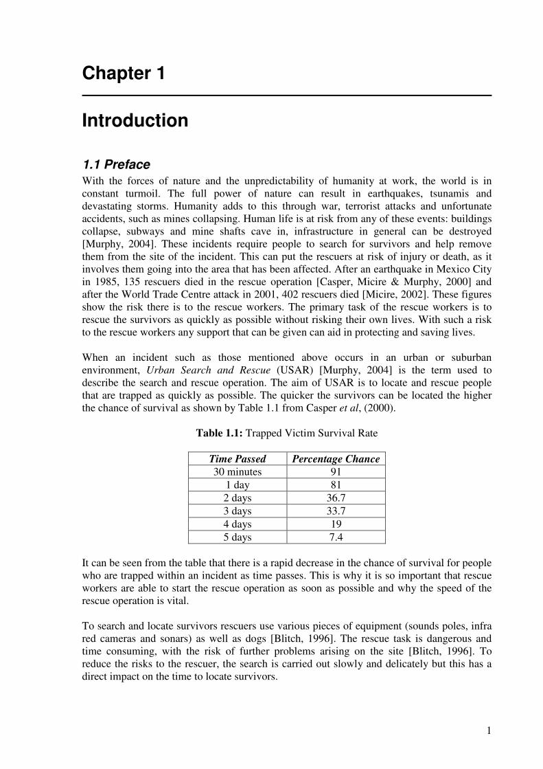
With the forces of nature and the unpredictability of humanity at work, the world is in constant turmoil. The full power of nature can result in earthquakes, tsunamis and devastating storms. Humanity adds to this through war, terrorist attacks and unfortunate accidents, such as mines collapsing. Human life is at risk from any of these events: buildings collapse, subways and mine shafts cave in, infrastructure in general can be destroyed [Murphy, 2004]. These incidents require people to search for survivors and help remove them from the site of the incident. This can put the rescuers at risk of injury or death, as it involves them going into the area that has been affected. After an earthquake in Mexico City in 1985, 135 rescuers died in the rescue operation [Casper, Micire & Murphy, 2000] and after the World Trade Centre attack in 2001, 402 rescuers died [Micire, 2002]. These figures show the risk there is to the rescue workers. The primary task of the rescue workers is to rescue the survivors as quickly as possible without risking their own lives. With such a risk to the rescue workers any support that can be given can aid in protecting and saving lives. When an incident such as those mentioned above occurs in an urban or suburban environment, Urban Search and Rescue (USAR) [Murphy, 2004] is the term used to describe the search and rescue operation. The aim of USAR is to locate and rescue people that are trapped as quickly as possible. The quicker the survivors can be located the higher the chance of survival as shown by Table 1.1 from Casper et al, (2000).
Table 1.1: Trapped Victim Survival Rate
Time Passed Percentage Chance
30 minutes 91 1 day 81 2 days 36.7 3 days 33.7 4 days 19 5 days 7.4
It can be seen from the table that there is a rapid decrease in the chance of survival for people who are trapped within an incident as time passes. This is why it is so important that rescue workers are able to start the rescue operation as soon as possible and why the speed of the rescue operation is vital. To search and locate survivors rescuers use various pieces of equipment (sounds poles, infra red cameras and sonars) as well as dogs [Blitch, 1996]. The rescue task is dangerous and time consuming, with the risk of further problems arising on the site [Blitch, 1996]. To reduce the risks to the rescuer, the search is carried out slowly and delicately but this has a direct impact on the time to locate survivors.
2
From the first time the word robot was used, in 1920 by Karel Čapek in Rossum’s Universal Robots [Čapek, 1920], the idea of the robot has been to act for humans in a whole range of tasks and environments. This concept of the use of a robot to act for humans naturally lends itself to the area of searching hazardous or large environments in place of or supporting human searchers. This is the underlying concept of this work: the use of a robot or a group of robots to search a hazardous environment.
1.2 Robotic Systems and Urban Search and Rescue
Since robots are able to act for humans in many tasks this leads to the argument that while robots are not yet advanced enough to recover survivors, they can be used as a tool to help locate the survivors [Blitch, 1996; Murphy, 2004]. The most obvious benefit of replacing rescue workers with robots is the decreased risk to the rescue workers, as they will then spend less time within the affected area. However there is a range of other benefits that are just as important [Blitch, 1996; Murphy, 2004]:
• Increased chance of locating survivors
Robots are able to enter smaller areas than humans and dogs [Blitch, 1996; Murphy, 2004; Birk & Carpin, 2006], and can operate without breaks. They do not suffer from fatigue, other than power running low. This increases the chance of locating survivors as the robots can operate for long periods in harsher conditions, but only if they are designed to do so.
• Less damage to affected area
If light robots are used on the affected area there will be less movement of rubble or other materials as there would be with humans and dogs [Murphy, 2004]. This movement can cause further damage to the site and increase the risk to survivors and rescue workers [Blitch, 1996].
• More information can be gained
While the robots are moving through the site, sensors on board can record a variety of information. This information can range from environmental readings to readings allowing the creation of maps of the site [Murphy, 2004; Murphy, Casper, Hyams, Micire and Minten, 2000b; Birk & Carpin, 2006]. This is desirable as any information can aid in the coordination of the rescue effort, decrease the risk to rescue workers and increase the speed of the search.
• The robot can go on the affected area instantly
Before rescue workers can go on site, an overall evaluation of the site needs to take place. Although this reduces slightly the chances of the survivors, it is designed to protect the rescue workers and aid in the overall rescue effort [Blitch, 1996; Murphy, 2004; Birk & Carpin, 2006]. Because robots are expendable they are able to go on to the site instantly, locating survivors from the start and hence guide the rescue operation at an earlier stage.
Consequently rescue robots can play an important role in rescue operations and as robots designs improve they are becoming a necessary tool for USAR [Murphy, 2004; Birk & Carpin, 2006].
3
1.3 Aims and Objectives of this work
The aim of this work is to establish if search algorithms can be used to generate points to allow a robot to search an environment for desired targets in a controlled manner. This work also aims to investigate whether using multiple robots, again under the direction of search algorithms, will impact on the time taken to search an environment and locate targets. The aim of this work can be summarised as:
• To establish if common search algorithms can be applied to generate points which enable a single robot or multiple robots to search an environment
• To present the algorithms which carry out this task well with supporting evidence
• To investigate if a better performance is achieved when the search algorithms are
extended to guide a group of robots To achieve the aim certain objectives need to be fulfilled. The first objective is the creation of a mathematical model of a mobile robot that will be used in an appropriate simulation to test the various search algorithms. This will provide the evidence needed to establish that the aim has been achieved. The second objective is to establish a suitable method of navigating and controlling the mobile robot. With suitable navigation and control the robot can respond correctly to the direction of the search algorithm used. With these objectives achieved the search algorithms that have been selected for study can be implemented in simulation in a single robot case and a multi robot case. A further addition of this work is the desire that the work is implemented on a real system. For this reason many design choices are constrained to ensure that the design can be implemented on a simple real system.
1.4 Contribution of this work
The work presented in this thesis is designed to contribute to the area of robotic search. The approach taken in this work is to establish if search algorithms can be used to generate points, allowing a robot to search an environment in a structured and controlled way. Currently there is no indication that this approach has been studied before and as such the application of search algorithms as a method of searching environments in this way is unique. However, this work takes this concept further by not only investigating if searches can be carried out but by also investigating if a search can be carried out using a group of robots and what benefits, if any, this brings to the search. The contributions of this work can be summarised as:
• Determination of whether common search algorithms can be used to guide a robot in a search of an environment
• The algorithms which perform this task efficiently and with the best results
• Whether the algorithms can be extended to provide guidance over multiple robots
An additional contribution of this work is the mathematical model that has been developed. Though mathematical models of mobile robots have been developed before, none offer six degrees of freedom, nor have any complete models been shown to have been validated.
4
To date the publications that have resulted from this work are as follows: Worrall, K.J. and McGookin, E.W., (2006), “A Mathematical Model of a Lego Differential Drive Robot “, 6th
UKACC Control Conference, Glasgow, UK The following papers are currently in preparation: Worrall, K.J., McGookin, E.W. and Macauley, M., “Mathematical model of a four wheeled mobile robot with Validation“ Worrall, K.J., McGookin, E.W. and Macauley, M., “Comparison of Control Methodologies on a small low speed four wheeled mobile robot“ Worrall, K.J., McGookin, E.W. and Macauley, M., “Using Tabu Random as a method of guiding mobile robots with regards to a search task “ Worrall, K.J., McGookin, E.W. and Macauley, M., “Comparison of Tabu Random and Simulated Annealing as a method of guiding a robot with regards to a search task“ Watts, C., Worrall, K.J., McGookin, E.W. and Macauley, M., “Low Cost IMU design “ These publications present the contributions of this work to the wider robotics community, allowing the work carried out to assist and inspire those working in similar areas.
1.5 Outline of thesis
This work proposes the use of robots to search environments under the control of search algorithms. The reasoning behind this approach is that that search algorithms are used in multiple fields of research and in industry to locate optimal points within a search space. In this application the optimal point will be the human survivors and the search space will be the USAR environment. The research carried out during the process of investigating this proposal is presented in this thesis using the structure described below. Chapter 2 introduces the major fields that this work is involved in: mobile robots within Urban Search and Rescue, mathematical models of mobile robots, control methodologies, and search algorithms. An overview of the work that is currently being done in these areas with respect to the work presented here is discussed. The first step in this work is to develop a mathematical model of a mobile robot which will allow a simulation to be created that can be used to test the search algorithms. The model is presented in Chapter 3. The model presented is a six degree of freedom model which includes the actuators. This model is also validated. With a suitable model developed the next stage is to develop a means of making the robot navigate and to select a suitable control methodology to allow the robot to be navigated accurately. Chapter 4 introduces the Line of Sight Autopilot technique of navigation and presents three control methodologies that could provide accurate control of the mobile robots forward velocity and heading: Proportional-Integral-Derivative, Pole Placement and Sliding
Mode. The obstacle avoidance method implemented is also discussed in Chapter 4.
5
The next step is to introduce the search algorithms that will be used to generate the coordinate points that the robot will be required to travel to. Chapter 5 introduces the Exhaustive, Random and HillCimbing searches, along with Simulated Annealing and Genetic
Algorithms. The use of Tabu search is also discussed and variations of the methods listed are introduced based on the Tabu search. This chapter presents the advantages of each algorithm and how each operates. Other matters concerning the way the robot searches an environment are also discussed, namely the ability of the robot to scan the temperature of the environment. The start of the simulation results that will support the conclusions of this work is presented in Chapter 6. This chapter discusses the simulation environments used in this work and how each method is implemented. The results from single agent cases of the search algorithms discussed in Chapter 5 are then presented and discussed. Chapter 7 presents the simulation results from the multi robot searches of the environments. The performances of the multi robot searches are discussed and the results from each search algorithms are presented along with suitable analysis. Chapter 8 concludes the thesis by stating the conclusions that can be drawn from the work carried out and reviewing the aims and objectives to show if the aim has been achieved and whether the objectives have been realised. Chapter 8 also discusses further work that can be done as a result of the work presented in this thesis.
6
Chapter 2
Literature Review
2.1 Introduction
The research carried out during the course of this work covered many different fields of research. This is the nature of robotic research, as robotics is a truly multi disciplinary field. One major research field that has been covered in this work is the application of robotic systems within Urban Search and Rescue (USAR). This is a relatively young area of research but in recent years this field has drawn more attention. The next area of research this work is concerned with is the modelling and simulation of dynamic systems with an emphasis on the development of models for mobile robots and the subsequent use of the modelled robot within suitable simulations. As such, a review of the mathematical models of mobile robots similar to that used in this work is presented in this chapter. As mentioned, a means of controlling the robot is required to allow it to travel to a requested point in a controlled manner. Control methodologies are another area of research this work covers. A review of the control methodologies that are investigated in this work is presented here, as this is the basis of how the robot is to move and hence achieve the task of locating targets within a given environment. The last research area this work covers is the field of optimisation. Though this has not yet been mentioned directly, the search algorithms studied in this work would be considered as optimisation methods. A general review of the search algorithms that are to be implemented is presented in this chapter. The chapter continues as follows: Section 2.2 presents an overview of mobile robot research with regards to USAR. Research literature which is concerned with mathematical models of mobile robots is presented in Section 2.3. This is followed by an overview of the research of control methodologies in Section 2.4. The chapter continues with Section 2.5 which presents work on the search algorithms presented in this thesis. Section 2.6 provides a brief summary of the chapter.
2.2 Mobile Robots within Urban Search and Rescue
The use of mobile robots within USAR would seem logical as robots can be used in areas where humans would be at risk. However it was only after the September 11th attacks on the World Trade Centre (WTC) in 2001 that research in this area started to gain momentum [Murphy, 2004; Ichbiah, 2005; Micire, 2002]. The reason for this is that the first deployment of robots within a USAR situation was at this event [Murphy, 2004; Ichbiah, 2005; Micire, 2002], though Blitch (1996) deployed robots at the Oklahoma City Bombing but this was only in the latter victim recovery operations. Since the deployment of robots at the WTC was deemed successful [Murphy, 2004; Micire, 2002] and the use of robots was accepted [Murphy, 2004], interest has increased in this field. It has been recognised that the development of robots for USAR poses many different challenges for research groups working in this area [Birk & Carpin, 2006] such as perception [Birk & Carpin, 2006], sensing [Murphy, 2004; Murphy et al, 2000b], world modelling [Birk & Carpin, 2006], locomotion [Murphy, 2004; Murphy, 2000a; Voyles & Larson, 2005; Murphy et al, 2000b;
7
Carlson & Murphy, 2005; Birk, Pathak, Schwertfeger and Chonnaparamutt, 2006], mapping [Birk & Carpin, 2006] and cooperation [Birk & Carpin, 2006; Jennings, Whelan and Evans, 1997; Dollarhide & Agah, 2003; Murphy, Lisetti, Tardif, Irish and Gage, 2002] to name but a few. This increased research also led to the creation of RoboCup Rescue [Kitano, Tadokaro, Noda, Matsubara, Takahashi, Shinjou and Shimada, 1999] as a sister competition to Robocup [Kitano, Asada, Kuniyoshi, Noda, Osawa and Matsubara, 1997] with the aim to help facilitate the application of laboratory research to the real world, to improve upon aspects of the RoboCup competition and to test real time teamwork in multi agent systems [Kitano et al, 1999]. The National Institute of Standards and Technology (NIST) also created a test bed to aid research within USAR [Murphy, Casper, Micire and Hyams, 2000c; Nourbakhsh, Sycara, Koes, Yong, Lewis and Burion, 2005]. This test bed offers three zones to test mobile robots with varying degrees of difficulty [Murphy et al, 2000c] with the zones simulating an office environment through to an area consisting of rubble. Further information on the NIST test bed can be found in Nourbakhsh et al (2005) and Murphy et al (2000). To further aid research of robotics within the USAR domain two major groups, Center for Robot Assisted Search and Rescue (CRASAR) at the University of South Florida [CRASAR, 2008] and the International Rescue System Institute in Japan [IRSI, 2008], have been set up with the purpose of researching robotic systems for USAR alongside other relevant research, such as Human-Robot Interaction [Murphy, 2004; Nourbakhsh et al, 2005]. Some believe that although autonomy is the “Holy Grail” [Birk & Carpin, 2006] for mobile robots, the use of fully autonomous systems is seen as “unrealistic…and undesirable” [Murphy, 2004]. This is because the demands on the robot are too great and rescue workers do not fully trust autonomous systems [Murphy, 2004]. Some believe that work within this field should concentrate on providing better systems and sensors for current mobile robots [Micire, 2002; Birk & Carpin, 2006]. It is generally accepted that a greater degree of autonomy with improved sensors and operator training will greatly enhance the use of robotic systems within USAR [Murphy, 2004; Birk & Carpin, 2006]. To overcome the issue of trust in using mobile robots within USAR, further successful deployments and awareness training [Murphy, 2004] will increase the desire for robots, as will describing the robots as tools that are to be used to assist the rescue effort [Blitch, 1996; Birk & Carpin, 2006]. With regards to a suitable mobile robot for USAR there exists a consensus amongst the available literature. A suitable robot should be:
• Small
The robot should be small in dimension and mass [Birk & Carpin, 2006; Murphy, 2004; Blitch, 1996]. A small robot will be able to enter areas of a search environment which will be inaccessible to humans or dogs [Murphy, 2004; Blitch, 1996]. A small, light robot can also be carried by a single person, making deployment easier [Birk & Carpin, 2006; Murphy, 2004; Blitch, 1996] .
• Expendable
As robots become more common within USAR the loss rate will increase due to the various challenges facing the robots within the working environment [Birk & Carpin, 2006]. Since losses are expected the current specialised systems used will be costly to replace, hence cheap expendable robots are required [Birk & Carpin, 2006].
8
• Useable
During the WTC USAR effort it was found that some of the robots donated to aid in the rescue could not be used due to either lack of training or lack of proper equipment for operating the robots [Micire, 2002; Murphy, 2004]. The robots used at the WTC USAR effort were all teleoperated and required operators that could use them [Micire, 2002; Murphy, 2004].
• Protection against Hazards
Within the working environment the robots will encounter various hazards: water, dust, fire, and blood are some examples [Murphy, 2004]. The robots are required to be protected in some way from these hazards as the operation of the robot could be adversely affected [Blitch, 1996; Murphy, 2004].
Many robots designed for the purpose of USAR are small light robots with either wheels or tracks providing locomotion, though there are many biologically inspired robots in existence, such as TerminatorBot [Voyles & Larson, 2005], which is able to crawl over obstacles, snake and serpentine robots [Murphy, 2000a; Murphy, 2000b; Ichbiah, 2005; Granosik & Borenstein, 2005; Tanev, Ray & Buller, 2005; Mori & Hirose, 2002]. This coincides with the list of desirable features stated above. However a further area of work within the field of mobile robots for USAR looks at the development of the mechanical aspects of the mobile robot. This has led to a number of different concepts. Since the environment the robot will be working in will be highly cluttered with a large number of different types of obstacles [Blitch, 1996], marsupial (where a ‘mother’ robot carries a smaller ‘child’ robot for deployment in areas where the mother can not go) and shape shifting robots [Murphy, 2000b] are being investigated for use within USAR. The research field of mobile robots within USAR is large, with many different research areas open for investigation. Even though so many different areas exist the conclusion reached in the majority of the work in this area is that mobile robots are an essential tool within USAR and their utilisation will increase considerably in the future [Birk & Carpin, 2006; Micire, 2002; Murphy, 2004; Blitch, 1996].
2.3 Mathematical Models of Mobile Robots
Mathematical modelling of systems has been commonplace since the first differential equations of the governors were developed in the early 19th Century [Bennet, 1996]. Since then mechanical, electrical and thermal systems, economics and biological systems have all been modelled [Ogata, 2002; Murray-Smith, 1995]. Larger complete systems have also been modelled, from marine vessels [Fossen, 1994; Alfaro-Cid, 2003; Perez, 2005] to aircraft [Cook, 1997] and satellites [Franklin, Powell & Emami-Naeini; 1991]. With a model of a system, tests and experiments can be carried out without any interaction with a real system. This is beneficial when the system under consideration is to be used, for example, in an aircraft. To test a system in a real aircraft would be expensive, time consuming and dangerous. Whereas a system tested on a mathematical representation of an aircraft will give similar results but without the cost, the length of time or the danger. This work will only consider more recent research concerned with mathematical models of mobile robots. Mathematical models of mobile robots can be divided into two major groups: Kinematic and Dynamic [Ge & Lewis, 2006; Hong, Ge, Lewis & Lee, 2006; Wang, Su & Ge, 2006]. A kinematic model is based only on the position and velocities of the robot, with the velocities
9
of the wheels acting as inputs [Ge & Lewis, 2006; Hong et al, 2006], whereas dynamic models describe the forces and moments acting on and generated by the robot. Kinematic models are the most popular, as indicated by the extensive literature that exists with kinematic models of mobile robots. Siegwart & Nourbakhsh (2004), Thurn, Burgard & Fox (2005), Astolfi (2006), Bruke & Durrant-Whyte (1993) and Minor, Albiston & Schwensen (2006) are some examples of work that develop kinematic based models of mobile robots. Dynamic models of mobile robots are popular but are often confined to papers. The reason for this could be the ease in which kinematic models can be created and manipulated and have variables which are readily understood, such as velocities. Dynamic models describe mobile robots with regards to the forces and moments acting on and being created by the robot and, therefore can be more difficult to use and interpret. Examples of dynamic mobile robot models can be found in Utkin, Guldner & Shi (1999), Hong et al (2006), Wang et al (2006), Worrall & McGookin (2006), Williams, Carter, Gallina & Rosati (2002), Albagul & Wahudi (2004) and Balakrishna & Ghosal (1995). Texts of interest within the area of mobile modelling are Ge & Lewis (2006), Williams et al (2002) and Balakrishma & Ghosal (1995). The advantages of developing mathematical models for robots include the design of subsystems (e.g. controllers) [Nehmzow, 2003; Lune, Spiess, & Röfer, 2005; Michel, 2004] and the ability to test repeatedly without the difficulty of a practical installation [Worrall & McGookin, 2006]. A common use of mathematical models is the design and evaluation of control systems for robot motion.
2.4 Control Methodologies
Control can be simply described as the process required to maintain a variable at a required value in the presence of disturbances and uncertainties [Ogata, 2002]. From James Watt’s steam engine governor, seen as the first step in control theory [Ogata, 2002; Bennet, 1996], a wide range of work has been published with regards to control theory, with many different control methodologies considered. For a historic overview of control consult Bennet (1996). The work presented here is concerned with three established control methodologies: Proportional-Integral-Derivative (PID) [Åström & Hägglund, 1995; Ogata, 2002; Cetinkunt, 2007; Franklin et al, 1991]; Pole Placement [Ogata, 2002; Philips & Harbor, 1996; Franklin et al, 1991] and Sliding Mode [Utkin et al, 1999; Edwards & Spurgeon, 1998; Young, Utkin & Özgüner, 1999; DeCarlo, Zak & Matthews 1988]. These methods were chosen due to the popularity of each of them, as indicated by the extensive literature available on each method.
2.4.1 Proportional-Integral-Derivative
PID control, also known as Classical Control or Three Term Control Controller, [Åström & Hägglund, 1995; Ogata, 2002; Cetinkunt, 2007; Franklin et al, 1991] is by far the best known and popular of the control methods that have been developed to date, as shown by the large number of publications associated with PID control. During the nineties Åström & Hägglund (1995) stated that more than 95% of process controls were PID and Cetinkunt (2007) states that 90% of controllers used are PID. These figures show that despite the variety of control methodologies available, PID controllers are still popular [Cetinkunt, 2007]. The reason for this popularity is the ease in which a basic PID controller can be implemented and the ability of the PID controller to generate an output which takes into consideration the past, current and future error [Cetinkunt, 2007]. Although a large range of literature is available on PID control, there is little difference between the basic PID presented in each. The literature is normally concerned with an application of the PID controller or a method of extending the PID controller to improve the
10
performance. A third topic that is covered in literature is methods of tuning PID controllers. The tuning of a PID controller is concerned with finding suitable controller values for the application that the controller is to be used in [Ogata, 2002]. PID controllers can be hand tuned [Ogata, 2002; Alfaro-Cid, 2003; Åström & Hägglund, 1995] where the controller values are achieved through a trial and error procedure. However there are tuning methods which are available to manually tune these values, the most popular of which is the Ziegler-Nichols method [Ziegler & Nichols, 1942; Åström & Hägglund, 1995; Ogata, 2002; Philips & Harbor, 1996; Dutton, Thompson & Barraclough, 1997; Dorf & Bishop, 2005; Franklin et
al, 1991]. The popularity of this method is shown by the literature that presents this method of tuning. It is acknowledged that though the Ziegler-Nichols method is effective, the values that it returns often require fine tuning [Ogata, 2002]. It is for this reason that other tuning methods are developed. An addition to this is the application of automatic tuning methods [Åström & Hägglund, 1995] which allow on demand tuning of controller values [Åström & Hägglund, 1995]. This has also led to adaptive PID controllers [Åström & Hägglund, 1995]. PID control is used in many different areas and a search for PID control on any of the major journals reveals hundreds of papers proposing applications of the PID controller or improvements to the PID controller. Further information on PID controllers can be found in a wide variety of literature, along with many examples of the use of PID controllers. One dedicated text is Åström & Hägglund (1995). Other texts include Ogata (2002), Cetinkunt (2007), Dutton et al (1997) and Dorf & Bishop (2005).
2.4.2 Pole Placement
Pole Placement [Ogata, 2002; Philips & Harbor, 1996; Dutton et al, 1997; Dorf & Bishop, 2005; White, 1995; Franklin et al, 1991] is the common name for State Variable Feedback
and Eigenstructure Assignment. The reason for this could be that State Variable
Feedback/Eigenstructure Assignment controllers are typically designed using the pole placement method. The use of Pole Placement creates a state feedback gain matrix [Ogata, 2002; Phillips & Harbor, 1996; Dorf & Bishop, 2005] that is used to feedback desirable current system states [Ogata, 2002; Dorf & Bishop, 2005]. By feeding back the states of the system through a gain matrix and comparing these to the desired states control inputs are created [Ogata, 2002]. The popularity of Pole Placement has led to the creation of various algorithms which calculate the state feedback gain matrix when given the system equations and desired poles. Two such algorithms are Ackermanns Formula [Dorf & Bishop, 2005; Philips & Harbor, 1996; Ogata, 2002], which is designed for single input systems [Ogata, 2002], and an algorithm developed by Kautsky, Nichols & Van Dooren (1985), both of which appear as commands within the MATLAB package [Ogata, 2002]. The algorithm developed by Kautsky et al (1985) can be used for both single input and multi input systems [Ogata, 2002]. The algorithm is designed to provide a robust solution to the pole placement problem, [Kautsky et al, 1985] giving a solution which is insensitive to perturbations [Kautsky et al, 1985]. One disadvantage of using the Pole Placement method to design a controller for a nonlinear system is that the algorithms presented above, which calculate the feedback matrix, require a linear model of the system to operate on [Ogata, 2002; Dutton et al 1997]. This involves the linearisation of the nonlinear model about a set point [Dutton et al, 1997]. As with PID control, Pole Placement is covered in a wide range of literature. Pole Placement control also returns hundreds of results when a search is carried out on the multitude of
11
journals available. The literature is wide ranging, from applications of a Pole Placement controller, such as vibration control [Sethi & Song, 2006], marine vessel control [Alfaro-Cid, McGookin & Murray-Smith, 2006; Alfaro-Cid, 2003], power circuit control [Kelly & Rinnie, 2005; Chow & Sanchez-Gasca, 1989], to improvements that can be made to controllers based on the Pole Placement principal. An overview of the field can be found in White (1995). A number of textbooks also cover simple controller design using Pole Placement: Dutton et al (1997), Ogata (2002), Philips & Harbor (1996) and Dorf & Bishop (2005).
2.4.3 Sliding Mode
Sliding Mode control [Utkin et al, 1999; Edwards & Spurgeon, 1998; Young et al, 1999; DeCarlo et al, 1988] is part of the Variable Structure Control work that came out from Russia during the 1970s [Young et al, 1999; Edwards & Spurgeon, 1998]. Sliding Mode controllers switch between two control laws [Young et al, 1999; Edwards & Spurgeon, 1998] during the operation of the controller. The main benefit of Sliding Mode control is its ability to handle variations in parameters and reject disturbances that may be introduced within the system from model uncertainties [DeCarlo et al, 1988; McGookin & Murray-Smith, 2006; Young et al, 1999]. However, a much cited disadvantage is the Chattering phenomenon [Young et al, 1999]. Chattering is the high frequency switching of the switching term about the sliding manifold [Young, et al 1999; Edwards & Spurgeon, 1998; Utkin et al, 1999]. The term chattering originates from the audible noise that sliding mode controllers exhibited in early implementations [Utkin et al, 1999]. Chattering is undesirable as it can cause unnecessary wear on actuators and power converters [Edwards & Spurgeon, 1998; McGookin, 1997]. Utkin et al (1999) suggest that the two main causes for chattering are fast dynamics that are unmodelled and the discretisation of signals within microcontrollers. Young et al (1999) suggest that chattering remains a major obstacle for a wider take-up of Sliding Mode control. Though acknowledged as an issue for Sliding Mode control, chattering can be reduced dramatically if handed correctly. The most common method used to reduce chattering is to smooth the switching that occurs within a boundary layer [Young et al, 1999] using soft
switching [Healey & Leinard, 1993; Alfaro-Cid, 2003; McGookin, 1997]. One method of soft switching is to replace the hard switching signum function [Edwards & Spurgeon, 1998; McGookin, 1997] with a hyperbolic tangent function [Alfaro-Cid 2003; Healey & Leinard, 1993; McGookin & Murray-Smith, 2006; McGookin, 1997]. In doing this the effect of chattering is reduced. Sliding Mode control can be found in a wide variety of fields: Marine Vessel control [McGookin & Murray-Smith, 2006; Alfaro-Cid, 2003; McGookin, Murray-Smith, Li & Fossen, 2000; McGookin, 1997], Electric drives [Utkin et al, 1999], Power Converters [Utkin et al, 1999], Robotics [Utkin et al, 1999], the control of swarms of robots [Gazi, 2005], formation control [Fahimi, 2007] and pneumatic system control [Nguyen, Leavitt, Jabbari & Bobrow, 2007]. As with the other controllers introduced within this section Sliding Mode has much literature associated with it. Dedicated texts are Edwards & Spurgeon (1998) and Utkin et al (1999). A tutorial for control engineers can be found in DeCarlo et al (1988).
12
2.5 Search Algorithms
The algorithms described as search algorithms in this work are also referred to as optimising
techniques or heuristic methods. The reason for the name search algorithms is related to the task that this work uses the algorithms for: that of locating a target within an environment with relation to the real world. A brief overview of the literature associated with each of the algorithms used in this work is given next.
2.5.1 Exhaustive Search
An Exhaustive Search, which can also be known as Brute Force [Johnson & Picton, 1995], is a very simple concept where every possible solution to a given problem is evaluated. This algorithm is seen as the most basic search algorithm and should only ever be used when only a small number of solutions exist for a problem, as a search through all possibilities would not be done in a reasonable time [Johnson & Picton, 1995]. Because of the impractical nature of exhaustive search there exists little literature concerning it. However, as a starting point for showing the advantages of other algorithms it is included here.
2.5.2 Random
As with the Exhaustive Search there exists little theoretical work on Random search algorithms. Random search algorithms are just as simple as the Exhaustive algorithm. The Random algorithm simply chooses solutions at random and tests those [Johnson & Picton, 1995]. This continues until such time as a stop condition is met. A close relative of the Random Algorithm would be the popular Monte Carlo Methods [Tarantola, 2005]. These methods are based on random numbers. However, the results of multiple random numbers are used to calculate a result with regards to Monte Carlo
Methods, [Tarantola, 2005] whereas a basic random algorithm does not consider other results. Research with regards to Random algorithms, within the robotics domain, includes path planning [Suzuki & Żyliński, 2008] and robot search [Cheng & Leng, 2004; Healey & Kim, 2000].
2.5.3 HillClimbing
The HillClimbing algorithm [Johnson & Picton, 1995; Russell & Norvig, 1995; Reeves, 1996] follows in a similar vein from the first two algorithms described. It is a very simple algorithm, however one that has attracted attention. The HillClimbing algorithm is also known as Gradient Ascent or Descent [Johnson & Picton, 1995; Russell & Norvig, 1995], Steepest Ascent [Johnson & Picton, 1995] or Neighbourhood Search [Reeves, 1996]. The problems associated with simple HillClimbing algorithms are widely reported with the most serious problem being that of the algorithm returning a local optima [Johnson & Picton, 1995; Russell & Norvig, 1995; Reeves, 1996]. Russell & Norvig (1995) suggest that the standard HillClimbing algorithm be altered to randomly select another solution when a near optimal solution of any kind is detected. This method would increase the chance of finding the global optimal region. Other work, for example Reeves (1996), suggests the use of other algorithms to overcome the HillClimbing algorithms failings. Some interesting application areas of the HillClimbing algorithm include search algorithms for Unmanned Air Vehicles (UAVs) [Zengin & Dogan, 2005], in the organisation of sporting tournaments [Lim, Rodrigues & Zhang, 2006] and image processing [Rambabu, Rathore & Chakrabarti, 2005].
13
2.5.4 Tabu
The Tabu algorithm [Glover, 1986; Glover, 1989; Reeves, 1996; Gendreau, 2003] was first proposed by Glover (1986). The Tabu algorithm is described as a metaheuristic [Glover, 1986; Glover, 1989; Reeves, 1996; Gendreau, 2003] as it is designed to run in support of another algorithm and direct its search. The main component of the Tabu algorithms is the Tabu List which is designed to maintain a list of solutions that have already been evaluated, hence stopping the primary algorithm from using those solutions again [Glover, 1986; Glover, 1989; Reeves, 1996; Gendreau, 2003]. Though the use of the Tabu algorithm to partner a primary algorithm takes up memory to allow the Tabu list, an advantage of its use is an ability to overcome the local optima convergence problem [Glover, 1989]. Tabu search also enables a more diverse search [Reeves, 1996] and enables better solutions to the problem to be located [Glover, 1989; Gendreau, 2003]. Tabu Search has been used in a wide range of areas: Integer Programming, computer scheduling, space planning, vehicle routing and traffic management systems [Glover, 1989; Gendreau, 2003]. Another area is within robot motion planning [Masehian & Amni-Naseri, 2008]. The primary references with regards to Tabu search are Glover (1986) and Glover (1989). Gendreau (2003) provides a good introduction of the Tabu Search.
2.5.5 Simulated Annealing
Simulated Annealing [Kirkpatrick, 1984; Bohachevsky, Johnson & Stein, 1986; Kirkpatrick, Gelatt & Vecchi, 1983; Johnson & Picton, 1995; Russell & Norvig, 1995; Reeves, 1996] is an algorithm which mimics the process of annealing [Bohachevsky et al, 1986; Kirkpatrick, 1984; Kirkpatrick et al, 1983; Johnson & Picton, 1995; Russell & Norvig, 1995; Reeves, 1996], a process in which a liquid is cooled until it becomes stable in a solid form [Bohachevsky et al, 1986; Kirkpatrick, 1984; Kirkpatrick et al, 1983; Johnson & Picton, 1995; Russell & Norvig, 1995; Reeves, 1996]. The original concept of the Simulated Annealing algorithm is credited to Metropolis, Rosenbluth, Rosenbluth and Teller (1953) [Bohachevsky et al, 1986; Reeves, 1996; McGookin, 1997]. The Simulated Annealing algorithm is loosely related to the HillClimbing algorithm as it carries out a local search [Bohachevsky et al, 1986; Russell & Norvig, 1995]. However, there are two major differences: the Annealing Schedule, also known as the cooling schedule
[Reeves, 1996; Johnson & Picton, 1995; McGookin, 1997; Bohachevsky et al, 1986], which varies the perturbations made by the algorithm [McGookin, 1997], and the Metropolis
Criterion [Metropolis et al, 1953; Bohachevsky et al, 1986; McGookin, 1997], which allows the algorithm to escape from local minima [McGookin, 1997]. The Annealing Schedule varies the perturbations made by the algorithm by reducing the size of the local neighbourhood. The Metropolis Criterion allows the algorithm to escape local optima by allowing poorer solutions to the current problem to be accepted [McGookin, 1997]. The Simulated Annealing algorithm has been used to optimise controllers for marine vessels [McGookin & Murray-Smith, 2006; McGookin, Murray-Smith, Li & Fossen, 2000; McGookin, 1997], to solve standard optimising problems such as the travelling salesman problem [Kirkpatrick et al, 1983; Bohachevsky et al, 1986], to aid in minimising power consumption in wireless communication [Montemanni, Gambardella & Das, 2005] and in the organisation of sporting tournaments [Lim et al, 2006; Anagnostopoulos, Van Hentenryck & Vergados, 2006]
14
Major texts for Simulated Annealing are Bohachevsky et al (1986), Kirkpatrick (1984), Kirkpatrick et al (1983) and Metropolis et al (1953).
2.5.6 Genetic Algorithms
Genetic Algorithms [Goldberg, 1989; Holland, 1992; Schmitt, 2004; Ellis, 1993; Mitchell, 1996; Reeves, 1996; Johnson & Picton, 1995] are based on Charles Darwin’s Theory of Evolution [Ellis, 1993; McGookin, 1997]. The creation of Genetic Algorithms is attributed to John Holland in the 1960’s [Mitchell, 1996]. The basic concept of Genetic Algorithms is that they mimic natural evolution. To do this Genetic Algorithms have a range of natural inspired operators (selection, crossover and mutation) [Holland, 1992; Schmitt, 2004; Ellis, 1993; Mitchell, 1996; Reeves, 1996]. Since the introduction of Genetic Algorithms there has been much research into various aspects of the Genetic Algorithm, as indicted by the vast number of papers, texts and conferences regarding Genetic Algorithms [Alfaro-Cid, 2003]. The methods used by each operator is one area were much research has been carried out. Some common operator methods are, for selection: Roulette wheel [Goldberg, 1989; Mitchell, 1996; Ellis, 1993; Reeves, 1996; Johnson & Picton, 1995; McGookin, 1997;], Tournament [Alfaro-Cid, 2003; McGookin, 1997;], Ranking [Mitchell, 1996; Alfaro-Cid, 2003] and Elitist [Mitchell, 1996; Alfaro-Cid, 2003; McGookin, 1997] and for crossover: uniform, one point, two point and multi point [Schmitt, 2004; Ellis, 1993; Mitchell, 1996; Reeves, 1996; Johnson & Picton, 1995; Alfaro-Cid, 2003; McGookin, 1997]. The methods noted here, as mentioned, are the more common methods but each year brings more diverse methods. Some examples are McDonald (2003) who proposed a new selection method called Genetic Farming; Hong, Wang & Chen (2000) studied applying multiple mutation rates; Hatta, Wakabayashi & Koide (2001) and Mušnjak & Golub (2004) investigated the use of elite individuals within a population. However the standard arrangement of the Genetic Algorithm remains common in much of the literature. Another common theme in Genetic Algorithm literature is the underlying theory. A good review of the theory behind Genetic Algorithms can be found in Mitchell (1996) with Schmitt (2003) also providing some theoretical background. Some texts which provide further details on Genetic Algorithms include Goldberg (1989), Mitchell (1996) and Ellis (1993).
2.6 Summary
This chapter has reviewed some of the relevant literature concerned with the major topics dealt with in this work. The major topics are defined as mobile robots within USAR, the development of mathematical models of mobile robots, control methodologies, namely PID, Pole Placement and Sliding Mode, and search algorithms. The search algorithms discussed were Exhaustive, Random, HillClimbing, Tabu, SA and GAs. This chapter directed the reader to literature that either originally created the concepts discussed or that provide a standard text within the field which will allow an interested party to become more familiar with the topic. Some recent work being done in each of the fields was also presented, along with applications of the topics discussed.
15
Chapter 3
Mathematical Model of a Suitable Mobile Robot
3.1 Introduction
The use of simulations in both academia and industry is common place with much of the research and initial experiments carried out first within simulation [Frankin et al, 1991; Murray-Smith, 1995; Nehmzow, 2003; Ogata, 2002]. Simulations allow the testing of theories, controllers and algorithms within controlled and repeatable circumstances [Murray-Smith, 1995]. This occurs as users can control aspects of the simulation allowing the simulation to remain constant between different runs or make changes to the simulation to test different aspects of what is being tested. Within robotics it is widely recognised that simulations of robots can be used to develop the design of subsystems (e.g. controllers) [Nehmzow, 2003; Lune, et al., 2005; Michel, 2004] quickly and test prototypes repeatedly without the difficulty of a practical installation [Worrall & McGookin, 2006] e.g. avoiding the complexities of altering code within the robotic platform at every iteration, or the time taken to develop a Hardware-in-the-Loop simulator. In addition to the robot itself, environmental aspects also influence experiments, e.g. ambient light and temperature levels. Sensors that are sensitive to light and temperature will behave differently if ambient levels have changed. The test environment may have also been altered with the addition or removal of obstacles. These aspects can all remain constant within a simulated environment resulting in a managed environment for experimental use. The robotic platform can also be guaranteed to remain constant within a simulation. The physical robotic platform will be subject to changes in the battery level as it is being used. Wear and tear may also be an issue and if a robotic platform is being used by a group of people, alterations may be made to the platform that may be unknown to the current user affecting the experiments. The constant nature of the simulation allows repeatable testing of code and setup and will allow comparisons to be made between different runs with different code or setup. This only allows a comparison with near ideal or ideal conditions. There are circumstances, such as the testing of sensors, where only testing on a physical system will provide true results. This shows that though simulation will allow extensive testing and provide a degree of confidence in any code written, simulation testing should be carried out in parallel with practical tests. Another advantage of the use of a simulation is that a group of robots can be simulated. This is advantageous when the research involves multi robot systems, as the robots need not exist, thus saving time and money. A simulation requires a mathematical model of the robot, which is a set of equations that describe the behaviour of the robot. Having the mathematical model is only the first step. Confidence in the accuracy of the results generated by the model is required. To achieve this, the model has to be validated against physical data from the actual vehicle being modelled. The model presented here is validated with results presented in Appendix A2. Having a validated model means that the user of the simulation can be confident that the results obtained from the simulated experiment are similar to those obtained from the physical robot [Murray-Smith, 1995]. The robotic system considered in this study is a four wheel mobile robot. The mathematical model used to describe the motion of such a robot contains two distinct aspects: the
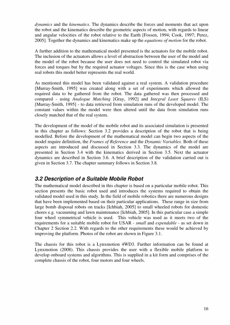
16
dynamics and the kinematics. The dynamics describe the forces and moments that act upon the robot and the kinematics describe the geometric aspects of motion, with regards to linear and angular velocities of the robot relative to the Earth [Fossen, 1994; Cook, 1997; Perez, 2005]. Together the dynamics and kinematics make up the equations of motion for the robot. A further addition to the mathematical model presented is the actuators for the mobile robot. The inclusion of the actuators allows a level of abstraction between the user of the model and the model of the robot because the user does not need to control the simulated robot via forces and torques but by the required actuator voltages. Since this is the case when using real robots this model better represents the real world. As mentioned this model has been validated against a real system. A validation procedure [Murray-Smith, 1995] was created along with a set of experiments which allowed the required data to be gathered from the robot. The data gathered was then processed and compared - using Analogue Matching [Gray, 1992] and Integral Least Squares (ILS) [Murray-Smith, 1995] - to data retrieved from simulation runs of the developed model. The constant values within the model were then altered until the data from simulation runs closely matched that of the real system. The development of the model of the mobile robot and its associated simulation is presented in this chapter as follows: Section 3.2 provides a description of the robot that is being modelled. Before the development of the mathematical model can begin two aspects of the model require definition, the Frames of Reference and the Dynamic Variables. Both of these aspects are introduced and discussed in Section 3.3. The dynamics of the model are presented in Section 3.4 with the kinematics derived in Section 3.5. Next the actuator dynamics are described in Section 3.6. A brief description of the validation carried out is given in Section 3.7. The chapter summary follows in Section 3.8.
3.2 Description of a Suitable Mobile Robot
The mathematical model described in this chapter is based on a particular mobile robot. This section presents the basic robot used and introduces the systems required to obtain the validated model used in this study. In the field of mobile robotics there are numerous designs that have been implemented based on their particular applications. These range in size from large bomb disposal robots on tracks [Ichbiah, 2005] to small wheeled robots for domestic chores e.g. vacuuming and lawn maintenance [Ichbiah, 2005]. In this particular case a simple four wheel symmetrical vehicle is used. This vehicle was used as it meets two of the requirements for a suitable mobile robot for USAR - small and expendable - as set down in Chapter 2 Section 2.2. With regards to the other requirements these would be achieved by improving the platform. Photos of the robot are shown in Figure 3.1. The chassis for this robot is a Lynxmotion 4WD3. Further information can be found at Lynxmotion (2008). This chassis provides the user with a flexible mobile platform to develop onboard systems and algorithms. This is supplied in a kit form and comprises of the complete chassis of the robot, four motors and four wheels.
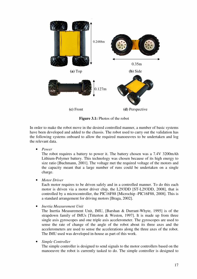
17
(a) Top (b) Side
(c) Front (d) Perspective
Figure 3.1: Photos of the robot In order to make the robot move in the desired controlled manner, a number of basic systems have been developed and added to the chassis. The robot used to carry out the validation has the following systems onboard to allow the required manoeuvres to be undertaken and log the relevant data.
• Power
The robot requires a battery to power it. The battery chosen was a 7.4V 3200mAh Lithium-Polymer battery. This technology was chosen because of its high energy to size ratio [Buchmann, 2001]. The voltage met the required voltage of the motors and the capacity meant that a large number of runs could be undertaken on a single charge.
• Motor Driver
Each motor requires to be driven safely and in a controlled manner. To do this each motor is driven via a motor driver chip, the L293DD [ST-L293DD, 2008], that is controlled by a microcontroller, the PIC16F88 [Microchip -PIC16F88, 2008]. This is a standard arrangement for driving motors [Braga, 2002].
• Inertia Measurement Unit
The Inertia Measurement Unit, IMU, [Barshan & Durrant-Whyte, 1995] is of the strapdown family of IMUs [Titterton & Weston, 1997]. It is made up from three single axis gyroscopes and one triple axis accelerometer. The gyroscopes are used to sense the rate of change of the angle of the robot about its three axes and the accelerometers are used to sense the accelerations along the three axes of the robot. The IMU used was developed in-house as part of this work.
• Simple Controller
The simple controller is designed to send signals to the motor controllers based on the manoeuvre the robot is currently tasked to do. The simple controller is designed to
0.35m
0.127m
0.2488m
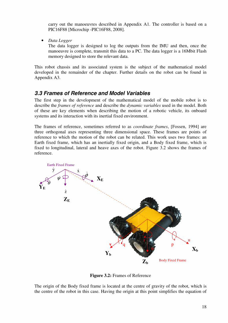
18
carry out the manoeuvres described in Appendix A1. The controller is based on a PIC16F88 [Microchip -PIC16F88, 2008].
• Data Logger
The data logger is designed to log the outputs from the IMU and then, once the manoeuvre is complete, transmit this data to a PC. The data logger is a 16Mbit Flash memory designed to store the relevant data.
This robot chassis and its associated system is the subject of the mathematical model developed in the remainder of the chapter. Further details on the robot can be found in Appendix A3.
3.3 Frames of Reference and Model Variables
The first step in the development of the mathematical model of the mobile robot is to describe the frames of reference and describe the dynamic variables used in the model. Both of these are key elements when describing the motion of a robotic vehicle, its onboard systems and its interaction with its inertial fixed environment. The frames of reference, sometimes referred to as coordinate frames, [Fossen, 1994] are three orthogonal axes representing three dimensional space. These frames are points of reference to which the motion of the robot can be related. This work uses two frames: an Earth fixed frame, which has an inertially fixed origin, and a Body fixed frame, which is fixed to longitudinal, lateral and heave axes of the robot. Figure 3.2 shows the frames of reference.
Figure 3.2: Frames of Reference
The origin of the Body fixed frame is located at the centre of gravity of the robot, which is the centre of the robot in this case. Having the origin at this point simplifies the equation of
Xb Yb
Zb
XE
ZE
YE
u v
w p q
r
x& y&
z&
φ& ψ&
θ&
Body Fixed Frame
Earth Fixed Frame
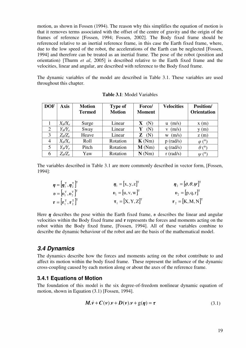
19
motion, as shown in Fossen (1994). The reason why this simplifies the equation of motion is that it removes terms associated with the offset of the centre of gravity and the origin of the frames of reference [Fossen, 1994; Fossen, 2002]. The Body fixed frame should be referenced relative to an inertial reference frame, in this case the Earth fixed frame, where, due to the low speed of the robot, the accelerations of the Earth can be neglected [Fossen, 1994] and therefore can be treated as an inertial frame. The pose of the robot (position and orientation) [Thurm et al, 2005] is described relative to the Earth fixed frame and the velocities, linear and angular, are described with reference to the Body fixed frame. The dynamic variables of the model are described in Table 3.1. These variables are used throughout this chapter.
Table 3.1: Model Variables
DOF Axis Motion
Termed
Type of
Motion
Force/
Moment
Velocities Position/
Orientation
1 Xb/Xe Surge Linear X (N) u (m/s) x (m) 2 Yb/Ye Sway Linear Y (N) v (m/s) y (m) 3 Zb/Ze Heave Linear Z (N) w (m/s) z (m) 4 Xb/Xe Roll Rotation K (Nm) p (rad/s) φ (°) 5 Yb/Ye Pitch Rotation M (Nm) q (rad/s) θ (°) 6 Zb/Ze Yaw Rotation N (Nm) r (rad/s) ψ (°)
The variables described in Table 3.1 are more commonly described in vector form, [Fossen, 1994]:
[ ]TT2
T1 ,ηηη = [ ]T
1 z,y,x=η [ ]T2 ,, ψθφ=η
[ ]TT2
T1 ,υυυ = [ ]T
1 w,v,u=υ [ ]T2 r,q,p=υ
[ ]TT2
T1 ,τττ = [ ]T
1 Z,Y,X=τ [ ]T2 N,M,K=τ
Here η describes the pose within the Earth fixed frame, υ describes the linear and angular velocities within the Body fixed frame and τ represents the forces and moments acting on the robot within the Body fixed frame, [Fossen, 1994]. All of these variables combine to describe the dynamic behaviour of the robot and are the basis of the mathematical model.
3.4 Dynamics
The dynamics describe how the forces and moments acting on the robot contribute to and affect its motion within the body fixed frame. These represent the influence of the dynamic cross-coupling caused by each motion along or about the axes of the reference frame.
3.4.1 Equations of Motion
The foundation of this model is the six degree-of-freedom nonlinear dynamic equation of motion, shown in Equation (3.1) [Fossen, 1994].
τηννDννCνM. =+++ )(g).().(& (3.1)
20
Here M is the mass and inertia matrix and C(υ) is the Coriolis matrix, which together represent the rigid model dynamics. D(υ) is the damping matrix, g(η) represents the gravitational forces and moments, and τ is a vector representing the control inputs [Fossen, 2002]. Each of these terms will be dealt with in the followings sections.
3.4.2 Rigid Body Dynamics
The robot is treated as a rigid body, which means it will be assumed that the robot’s mass and shape does not alter, though this is an idealised concept [Young & Freedman, 2000] as no fuel is used and there is no loss of mass as the robot moves. The rigid body dynamics describe the equations that allow the rigid body to move when a force is applied. The equations are based on the Newton-Euler formulation for rigid bodies [Fossen, 1994; Fossen, 2002]. The Newton-Euler formulation is based on Newton’s second law which states that mass multiplied by the acceleration equals the unbalanced forces acting on the body, represented by [Young & Freedman, 2000]:
∑= Farr
.m (3.2) Where m is the mass, kg, a
r is an acceleration, ms
-2, and ∑Fr
is the sum of the forces acting on the body, N. To develop the equations of motion Euler’s first and second axioms are used [Fossen, 1994]. These represent Newton’s second law in terms of the conversation of momentum. Euler’s first and second axioms are:
cc fprr
= cc .m vprr
= (3.3)
cc mhrr
= ibcc .whrr
I= (3.4)
where cpr
is linear momentum, chv
is angular momentum, cfr
and cmr
are the forces and
moments acting on the centre of gravity of the rigid body, m is mass, kg, cvv
is the velocity at
the centre of gravity, ibwr
is the angular velocity of frame b relative to i and Ic is the inertia dyadic, which is the inertia matrix about the centre of gravity [Fossen, 2002]. The proof of how Newton’s Second Law and Euler’s First and Second Axiom become the rigid body equations of motion can be found in Fossen (1994) and Fossen (2002). The rigid body equations of motion, with the origin of the body fixed frame at the centre of gravity and coinciding with the principal axes of inertia, of the robot can be stated as [Fossen, 1994; Fossen, 2002]:
Nq.p).II(r.I
Mp.r).II(q.I
Kr.q).II(p.I
Z)p.vq.uw.(m
Y)r.up.wv.(m
X)q.wr.vu.(m
xcyczc
zcxcyc
yczcxc
=−+
=−+
=−+
=+−
=+−
=+−
&
&
&
&
&
&
(3.5)
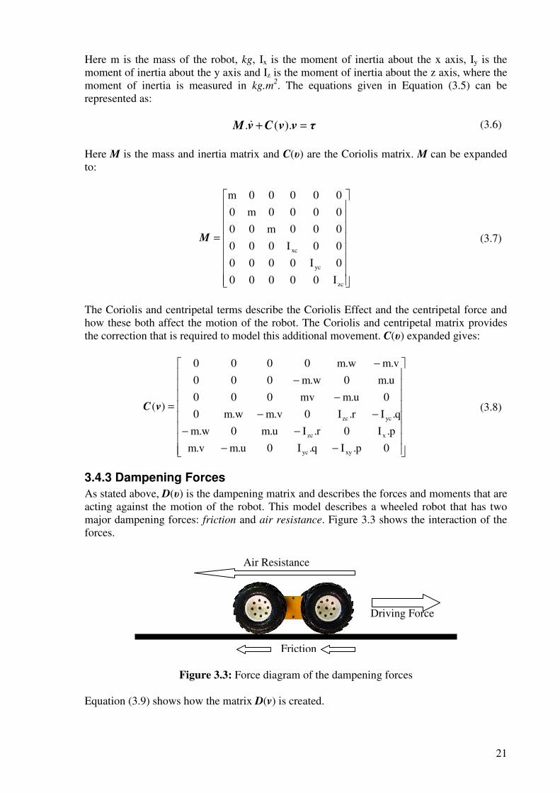
21
Here m is the mass of the robot, kg, Ix is the moment of inertia about the x axis, Iy is the moment of inertia about the y axis and Iz is the moment of inertia about the z axis, where the moment of inertia is measured in kg.m
2. The equations given in Equation (3.5) can be represented as:
τννCνM =+ ).(.& (3.6)
Here M is the mass and inertia matrix and C(υ) are the Coriolis matrix. M can be expanded to:
=
zc
yc
xc
I00000
0I0000
00I000
000m00
0000m0
00000m
M (3.7)
The Coriolis and centripetal terms describe the Coriolis Effect and the centripetal force and how these both affect the motion of the robot. The Coriolis and centripetal matrix provides the correction that is required to model this additional movement. C(υ) expanded gives:
−−
−−
−−
−
−
−
=
0p.Iq.I0u.mv.m
p.I0r.Iu.m0w.m
q.Ir.I0v.mw.m0
0u.mmv000
u.m0w.m000
v.mw.m0000
)(
xyyc
xzc
yczc
νC (3.8)
3.4.3 Dampening Forces
As stated above, D(υ) is the dampening matrix and describes the forces and moments that are acting against the motion of the robot. This model describes a wheeled robot that has two major dampening forces: friction and air resistance. Figure 3.3 shows the interaction of the forces.
Figure 3.3: Force diagram of the dampening forces
Equation (3.9) shows how the matrix D(v) is created.
Air Resistance
Driving Force
Friction
22
)(F)(F)( arf vvvD += (3.9) Here Ff is a vector representing the frictional forces and moments and Far is a vector describing the forces and moments occurring due to air resistance. 3.4.3.1 Friction
The robot runs on wheels and as a result the frictional force is termed rolling friction [Jellet, 1872]. The coefficient of friction associated with rolling friction is lower than that of static or kinetic friction. The standard equation for friction is [Young & Freedman, 2000]:
σ= .g.mFf (3.10)
where Ff is the frictional force, N, m is the mass of the robot, kg, g is the acceleration due to gravity and σ is the coefficient of rolling friction. Each axis has a component of friction acting against the motion along or about it. The friction coefficients associated with the motions are different for each axis, as the motion along or about each axis has to overcome different resistive forces or moments. During the validation procedure it has been found that an additional variable is required in the standard friction equation. The variable required is the appropriate velocity along or about the axis that the friction exists on. Equation (3.11) shows the vector that describes Ff(ν).
=
r
q
p
z
y
x
f
mr.r..W
mr.q..W
mr.p..W
w..W
v..W
u..W
)ν(F ψθφσ
σ
σ
σ
σ
σ
(3.11)
In this case W is the weight of the robot, N, σ# is the friction coefficient along or about the axis #, where # is either x, y, z, φ, θ or ψ, the velocities are as stated before and mrς is the moment arm, m, that transforms the forces into torques, with ς representing p, q or r.
3.4.3.2 Air Resistance
As the robot moves through air it meets resistance that causes drag. The drag can be calculated using the following [Hoerner, 1965]:
2ardar v..A.C.5.0F ρ= (3.12)
here Far is the force produced, N, Cd is the drag coefficient, A is the surface area presented to the direction of travel, m2, ρ is the density of air, 1.29 kg.m
-3 and var is the velocity acting in the direction of travel, ms
-1. The drag coefficient is a number that is based on the shape of the robot. Though a simplification, the shape of the robot presented here is given as a cuboid, giving a drag coefficient of 0.89 [Hoerner, 1965].
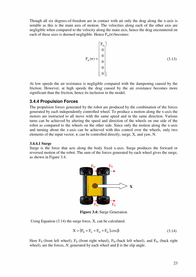
23
Though all six degrees-of-freedom are in contact with air only the drag along the x-axis is notable as this is the main axis of motion. The velocities along each of the other axis are negligible when compared to the velocity along the main axis, hence the drag encountered on each of these axes is deemed negligible. Hence Far(v) becomes:
=
0
0
0
0
0
F
)(F
ar
ar v (3.13)
At low speeds the air resistance is negligible compared with the dampening caused by the friction. However, at high speeds the drag caused by the air resistance becomes more significant than the friction, hence its inclusion in the model.
3.4.4 Propulsion Forces
The propulsion forces generated by the robot are produced by the combination of the forces generated by each independently controlled wheel. To produce a motion along the x-axis the motors are instructed to all move with the same speed and in the same direction. Various turns can be achieved by altering the speed and direction of the wheels on one side of the robot as compared to the wheels on the other side. Since only the motion along the x-axis and turning about the z-axis can be achieved with this control over the wheels, only two elements of the input vector, τ, can be controlled directly, surge, X, and yaw, N. 3.4.4.1 Surge
Surge is the force that acts along the body fixed x-axis. Surge produces the forward or reversed motion of the robot. The sum of the forces generated by each wheel gives the surge, as shown in Figure 3.4.
Figure 3.4: Surge Generation
Using Equation (3.14) the surge force, X, can be calculated.
( ) β+++= cos.FFFFX brblfrfl (3.14) Here Ffl (front left wheel), Ffr (front right wheel), Fbl (back left wheel), and Fbr, (back right wheel), are the forces, N, generated by each wheel and β is the slip angle.
Ffl Fbl
Ffr Fbr
X
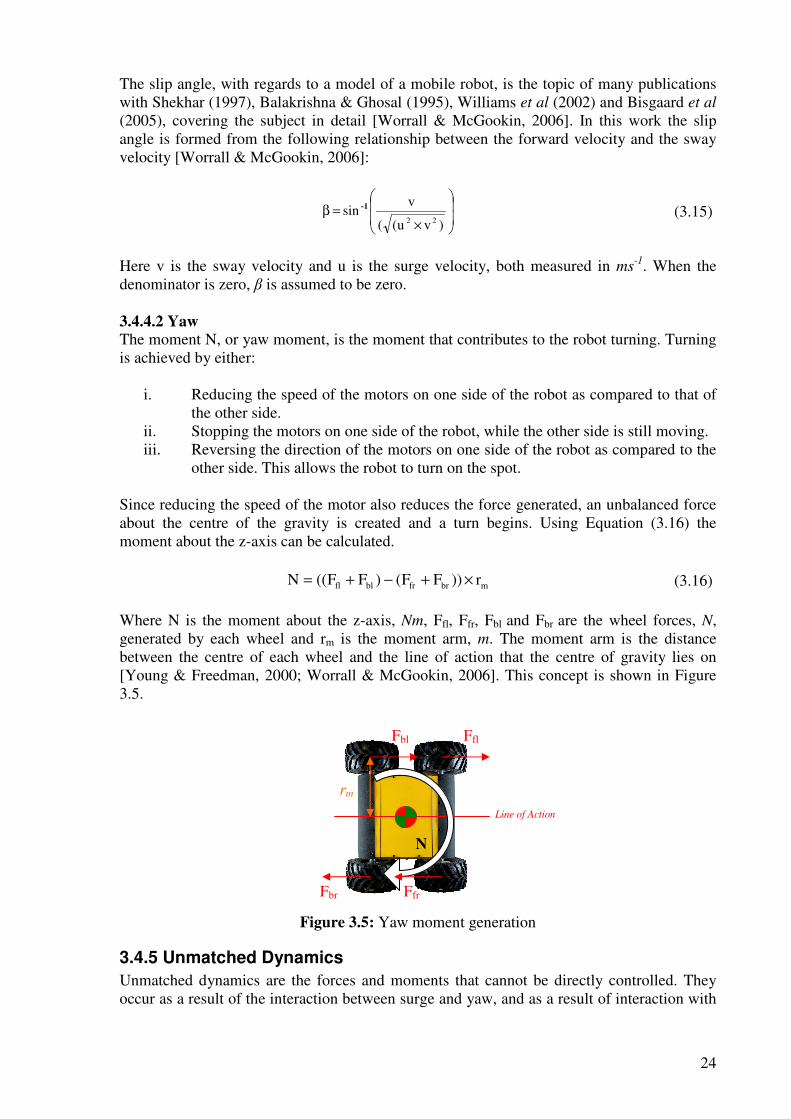
24
The slip angle, with regards to a model of a mobile robot, is the topic of many publications with Shekhar (1997), Balakrishna & Ghosal (1995), Williams et al (2002) and Bisgaard et al (2005), covering the subject in detail [Worrall & McGookin, 2006]. In this work the slip angle is formed from the following relationship between the forward velocity and the sway velocity [Worrall & McGookin, 2006]:
×=β
)vu((
vsin
22
1- (3.15)
Here v is the sway velocity and u is the surge velocity, both measured in ms
-1. When the denominator is zero, β is assumed to be zero. 3.4.4.2 Yaw
The moment N, or yaw moment, is the moment that contributes to the robot turning. Turning is achieved by either:
i. Reducing the speed of the motors on one side of the robot as compared to that of the other side.
ii. Stopping the motors on one side of the robot, while the other side is still moving. iii. Reversing the direction of the motors on one side of the robot as compared to the
other side. This allows the robot to turn on the spot. Since reducing the speed of the motor also reduces the force generated, an unbalanced force about the centre of the gravity is created and a turn begins. Using Equation (3.16) the moment about the z-axis can be calculated.
mbrfrblfl r))FF()FF((N ×+−+= (3.16) Where N is the moment about the z-axis, Nm, Ffl, Ffr, Fbl and Fbr are the wheel forces, N, generated by each wheel and rm is the moment arm, m. The moment arm is the distance between the centre of each wheel and the line of action that the centre of gravity lies on [Young & Freedman, 2000; Worrall & McGookin, 2006]. This concept is shown in Figure 3.5.
Figure 3.5: Yaw moment generation
3.4.5 Unmatched Dynamics
Unmatched dynamics are the forces and moments that cannot be directly controlled. They occur as a result of the interaction between surge and yaw, and as a result of interaction with
Ffl Fbl
Ffr Fbr
N
Line of Action
rm
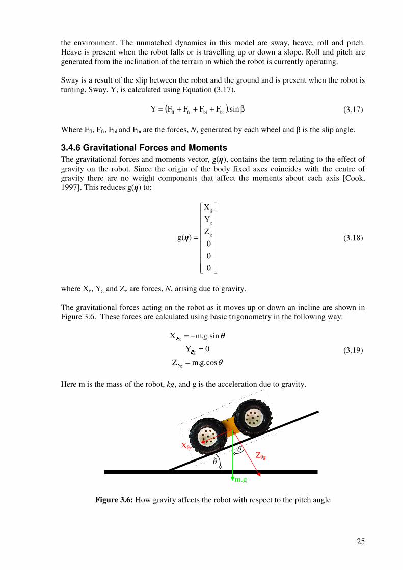
25
the environment. The unmatched dynamics in this model are sway, heave, roll and pitch. Heave is present when the robot falls or is travelling up or down a slope. Roll and pitch are generated from the inclination of the terrain in which the robot is currently operating. Sway is a result of the slip between the robot and the ground and is present when the robot is turning. Sway, Y, is calculated using Equation (3.17).
( ) β+++= sin.FFFFY brblfrfl (3.17) Where Ffl, Ffr, Fbl and Fbr are the forces, N, generated by each wheel and β is the slip angle.
3.4.6 Gravitational Forces and Moments
The gravitational forces and moments vector, g(η), contains the term relating to the effect of gravity on the robot. Since the origin of the body fixed axes coincides with the centre of gravity there are no weight components that affect the moments about each axis [Cook, 1997]. This reduces g(η) to:
=
0
0
0
Z
Y
X
)(g g
g
g
η (3.18)
where Xg, Yg and Zg are forces, N, arising due to gravity. The gravitational forces acting on the robot as it moves up or down an incline are shown in Figure 3.6. These forces are calculated using basic trigonometry in the following way:
θ
θ
cos.g.mZ
0Y
sin.g.mX
g
g
g
=
=
−=θ θθ (3.19)
Here m is the mass of the robot, kg, and g is the acceleration due to gravity.
Figure 3.6: How gravity affects the robot with respect to the pitch angle
m.g
Zθg Xθg
θ
θ
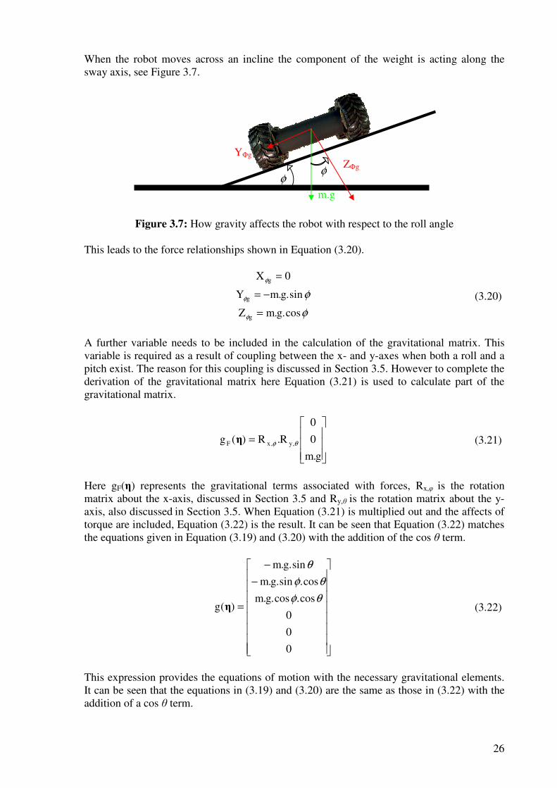
26
When the robot moves across an incline the component of the weight is acting along the sway axis, see Figure 3.7.
Figure 3.7: How gravity affects the robot with respect to the roll angle
This leads to the force relationships shown in Equation (3.20).
φ
φ
φ
φ
φ
cos.g.mZ
sin.g.mY
0X
g
g
g
=
−=
=
(3.20)
A further variable needs to be included in the calculation of the gravitational matrix. This variable is required as a result of coupling between the x- and y-axes when both a roll and a pitch exist. The reason for this coupling is discussed in Section 3.5. However to complete the derivation of the gravitational matrix here Equation (3.21) is used to calculate part of the gravitational matrix.
=
g.m
0
0
R.R)(g ,y,xF θφη (3.21)
Here gF(η) represents the gravitational terms associated with forces, Rx,φ is the rotation matrix about the x-axis, discussed in Section 3.5 and Ry,θ is the rotation matrix about the y-axis, also discussed in Section 3.5. When Equation (3.21) is multiplied out and the affects of torque are included, Equation (3.22) is the result. It can be seen that Equation (3.22) matches the equations given in Equation (3.19) and (3.20) with the addition of the cos θ term.
−
−
=
0
0
0
cos.cos.g.m
cos.sin.g.m
sin.g.m
)(gθφ
θφ
θ
η (3.22)
This expression provides the equations of motion with the necessary gravitational elements. It can be seen that the equations in (3.19) and (3.20) are the same as those in (3.22) with the addition of a cos θ term.
m.g
ZΦg
YΦg
φ
φ
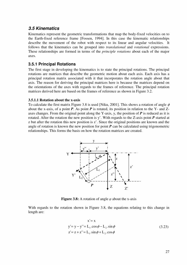
27
3.5 Kinematics
Kinematics represent the geometric transformations that map the body-fixed velocities on to the Earth-fixed reference frame [Fossen, 1994]. In this case the kinematic relationships describe the movement of the robot with respect to its linear and angular velocities. It follows that the kinematics can be grouped into translational and rotational expressions. These relationships are formed in terms of the principle rotations about each of the major axes.
3.5.1 Principal Rotations
The first stage in developing the kinematics is to state the principal rotations. The principal rotations are matrices that describe the geometric motion about each axis. Each axis has a principal rotation matrix associated with it that incorporates the rotation angle about that axis. The reason for deriving the principal matrices here is because the matrices depend on the orientations of the axes with regards to the frames of reference. The principal rotation matrices derived here are based on the frames of reference as shown in Figure 3.2. 3.5.1.1 Rotation about the x-axis
To calculate the first matrix Figure 3.8 is used [Niku, 2001]. This shows a rotation of angle φ about the x-axis, of a point P. As point P is rotated, its position in relation to the Y- and Z-axes changes. From the original point along the Y-axis, y, the position of P is reduced as it is rotated. After the rotation the new position is y’. With regards to the Z-axis point P started at z but after the rotation this new position is z’. Since the original positions are known and the angle of rotation is known the new position for point P can be calculated using trigonometric relationships. This forms the basis on how the rotation matrices are created.
Figure 3.8: A rotation of angle φ about the x-axis
With regards to the rotation shown in Figure 3.8, the equations relating to this change in length are:
φφ
φφ
cos.Lsin.L''zz'z
sin.Lcos.L''yy'y
x'x
21
21
+=+=
−=−=
=
(3.23)
Z Z’
Y’
Y φ
φ
P
z’
z”
z
y’ y”
y
L1
L2
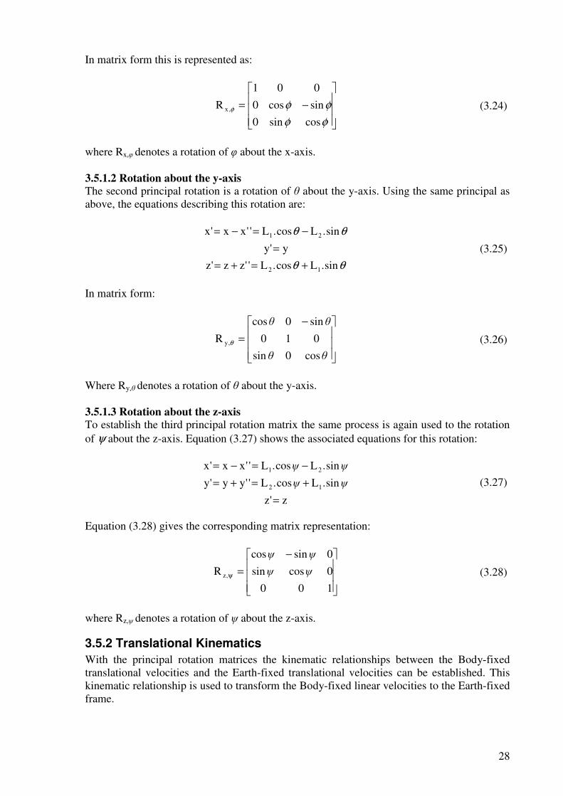
28
In matrix form this is represented as:
−=
φφ
φφφ
cossin0
sincos0
001
R ,x (3.24)
where Rx,φ denotes a rotation of φ about the x-axis. 3.5.1.2 Rotation about the y-axis
The second principal rotation is a rotation of θ about the y-axis. Using the same principal as above, the equations describing this rotation are:
θθ
θθ
sin.Lcos.L''zz'z
y'y
sin.Lcos.L''xx'x
12
21
+=+=
=
−=−=
(3.25)
In matrix form:
−
=
θθ
θθ
cos0sin
010
sin0cos
R ,y θ (3.26)
Where Ry,θ denotes a rotation of θ about the y-axis. 3.5.1.3 Rotation about the z-axis
To establish the third principal rotation matrix the same process is again used to the rotation of ψ about the z-axis. Equation (3.27) shows the associated equations for this rotation:
z'z
sin.Lcos.L''yy'y
sin.Lcos.L''xx'x
12
21
=
+=+=
−=−=
ψψ
ψψ
(3.27)
Equation (3.28) gives the corresponding matrix representation:
−
=ψ
100
0cossin
0sincos
R ,z ψψ
ψψ
(3.28)
where Rz,ψ denotes a rotation of ψ about the z-axis.
3.5.2 Translational Kinematics
With the principal rotation matrices the kinematic relationships between the Body-fixed translational velocities and the Earth-fixed translational velocities can be established. This kinematic relationship is used to transform the Body-fixed linear velocities to the Earth-fixed frame.
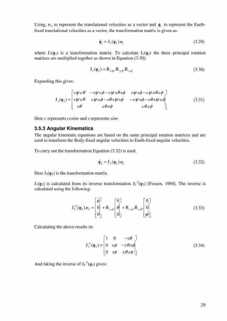
29
Using, ν1, to represent the translational velocities as a vector and 1η& to represent the Earth-fixed translational velocities as a vector, the transformation matrix is given as:
1211 ).(J υηη =& (3.29)
where J1(η2) is a transformation matrix. To calculate J1(η2) the three principal rotation matrices are multiplied together as shown in Equation (3.30).
φθψ ,x,y,z21 R.R.R)(J =η (3.30) Expanding this gives:
−−−
−−−
=
φθφθθ
φψθφψφψθφψθψ
φθψφψφθψφψθψ
c.cs.cs
c.s.ss.cs.s.sc.cc.s
c.s.cs.ss.s.cc.sc.c
)(J 21 η (3.31)
Here c represents cosine and s represents sine.
3.5.3 Angular Kinematics
The angular kinematic equations are based on the same principal rotation matrices and are used to transform the Body-fixed angular velocities to Earth-fixed angular velocities. To carry out the transformation Equation (3.32) is used.
2222 ).(J υηη =& (3.32) Here J2(η2) is the transformation matrix. J1(η2) is calculated from its inverse transformation J2
-1(η2) [Fossen, 1994]. The inverse is calculated using the following:
+
+
=−
ψ
θ
φ
θφφ
&
&
&
0
0
.R.R
0
0
.R
0
0).(J ,y,x,x221
2 υη (3.33)
Calculating the above results in:
−
−
=−
φθφ
φθφ
θ
c.cs0
s.cc0
s01
)(J 21
2 η (3.34)
And taking the inverse of J2-1(η2) gives:
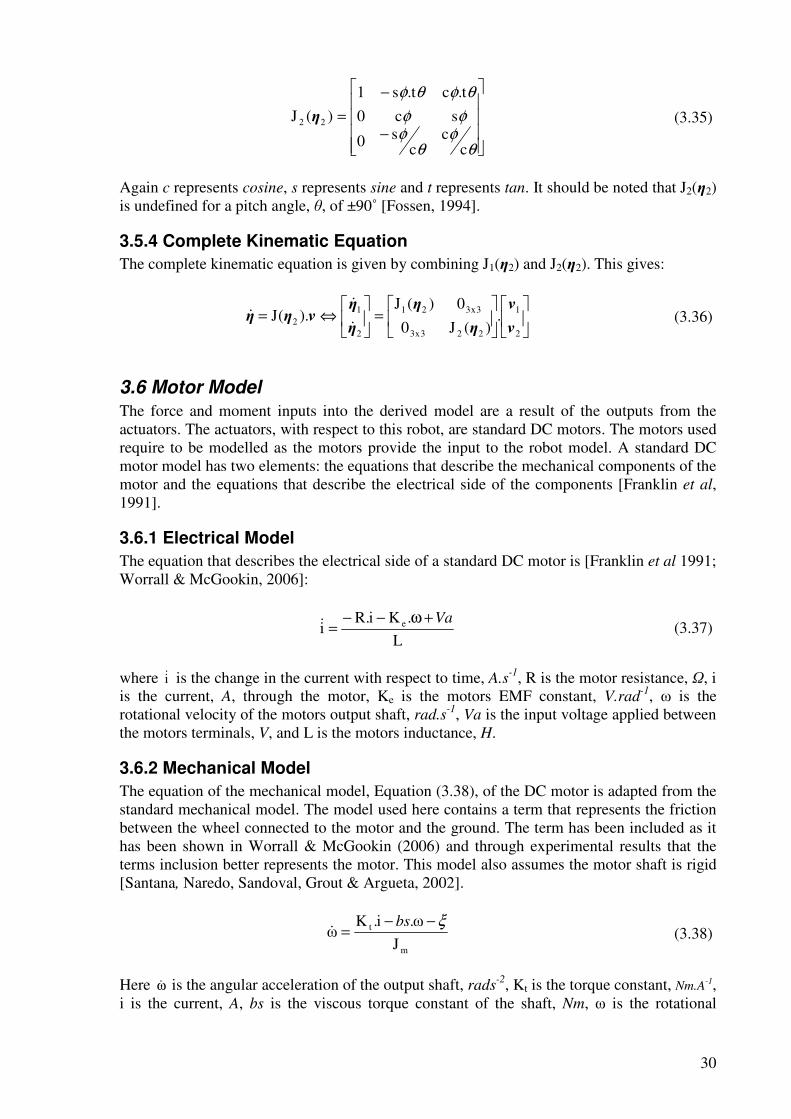
30
−
−
=
θφ
θφ
φφ
θφθφ
cc
cs0
sc0
t.ct.s1
)(J 22 η (3.35)
Again c represents cosine, s represents sine and t represents tan. It should be noted that J2(η2) is undefined for a pitch angle, θ, of ±90˚ [Fossen, 1994].
3.5.4 Complete Kinematic Equation
The complete kinematic equation is given by combining J1(η2) and J2(η2). This gives:
=
⇔=
2
1
223x3
3x321
2
12 .
)(J0
0)(J).(J
ν
ν
η
η
η
ηνηη
&
&& (3.36)
3.6 Motor Model
The force and moment inputs into the derived model are a result of the outputs from the actuators. The actuators, with respect to this robot, are standard DC motors. The motors used require to be modelled as the motors provide the input to the robot model. A standard DC motor model has two elements: the equations that describe the mechanical components of the motor and the equations that describe the electrical side of the components [Franklin et al, 1991].
3.6.1 Electrical Model
The equation that describes the electrical side of a standard DC motor is [Franklin et al 1991; Worrall & McGookin, 2006]:
L
.Ki.Ri e Va+ω−−
=& (3.37)
where i& is the change in the current with respect to time, A.s
-1, R is the motor resistance, Ω, i is the current, A, through the motor, Ke is the motors EMF constant, V.rad
-1, ω is the rotational velocity of the motors output shaft, rad.s
-1, Va is the input voltage applied between the motors terminals, V, and L is the motors inductance, H.
3.6.2 Mechanical Model
The equation of the mechanical model, Equation (3.38), of the DC motor is adapted from the standard mechanical model. The model used here contains a term that represents the friction between the wheel connected to the motor and the ground. The term has been included as it has been shown in Worrall & McGookin (2006) and through experimental results that the terms inclusion better represents the motor. This model also assumes the motor shaft is rigid [Santana, Naredo, Sandoval, Grout & Argueta, 2002].
m
t
J
ω.i.Kω
ξ−−=
bs& (3.38)
Here ω& is the angular acceleration of the output shaft, rads
-2, Kt is the torque constant, Nm.A-1,
i is the current, A, bs is the viscous torque constant of the shaft, Nm, ω is the rotational
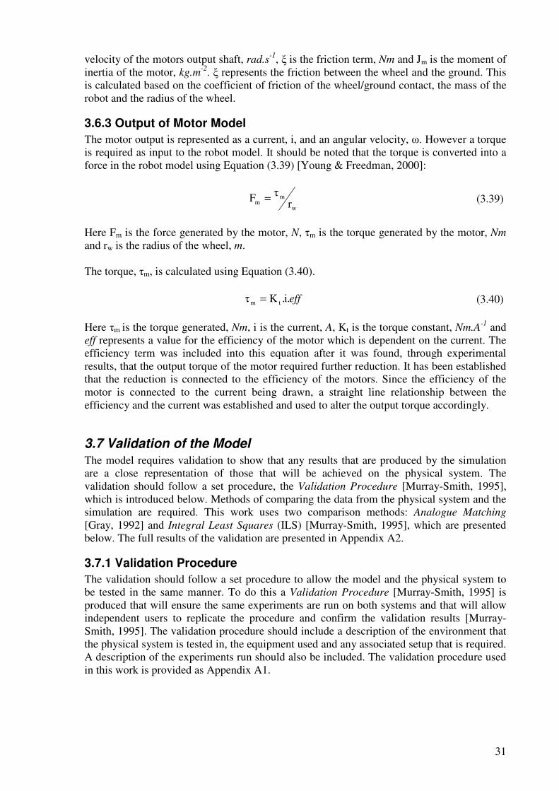
31
velocity of the motors output shaft, rad.s-1, ξ is the friction term, Nm and Jm is the moment of
inertia of the motor, kg.m-2. ξ represents the friction between the wheel and the ground. This
is calculated based on the coefficient of friction of the wheel/ground contact, the mass of the robot and the radius of the wheel.
3.6.3 Output of Motor Model
The motor output is represented as a current, i, and an angular velocity, ω. However a torque is required as input to the robot model. It should be noted that the torque is converted into a force in the robot model using Equation (3.39) [Young & Freedman, 2000]:
w
mm r
τF = (3.39)
Here Fm is the force generated by the motor, N, τm is the torque generated by the motor, Nm and rw is the radius of the wheel, m. The torque, τm, is calculated using Equation (3.40).
eff.i.Kτ tm = (3.40)
Here τm is the torque generated, Nm, i is the current, A, Kt is the torque constant, Nm.A-1 and
eff represents a value for the efficiency of the motor which is dependent on the current. The efficiency term was included into this equation after it was found, through experimental results, that the output torque of the motor required further reduction. It has been established that the reduction is connected to the efficiency of the motors. Since the efficiency of the motor is connected to the current being drawn, a straight line relationship between the efficiency and the current was established and used to alter the output torque accordingly.
3.7 Validation of the Model
The model requires validation to show that any results that are produced by the simulation are a close representation of those that will be achieved on the physical system. The validation should follow a set procedure, the Validation Procedure [Murray-Smith, 1995], which is introduced below. Methods of comparing the data from the physical system and the simulation are required. This work uses two comparison methods: Analogue Matching [Gray, 1992] and Integral Least Squares (ILS) [Murray-Smith, 1995], which are presented below. The full results of the validation are presented in Appendix A2.
3.7.1 Validation Procedure
The validation should follow a set procedure to allow the model and the physical system to be tested in the same manner. To do this a Validation Procedure [Murray-Smith, 1995] is produced that will ensure the same experiments are run on both systems and that will allow independent users to replicate the procedure and confirm the validation results [Murray-Smith, 1995]. The validation procedure should include a description of the environment that the physical system is tested in, the equipment used and any associated setup that is required. A description of the experiments run should also be included. The validation procedure used in this work is provided as Appendix A1.
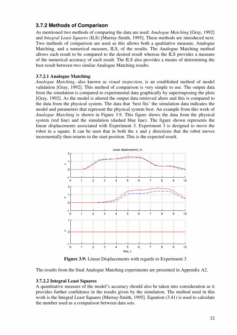
32
3.7.2 Methods of Comparison
As mentioned two methods of comparing the data are used: Analogue Matching [Gray, 1992] and Integral Least Squares (ILS) [Murray-Smith, 1995]. These methods are introduced next. Two methods of comparison are used as this allows both a qualitative measure, Analogue Matching, and a numerical measure, ILS, of the results. The Analogue Matching method allows each result to be compared to the desired result whereas the ILS provides a measure of the numerical accuracy of each result. The ILS also provides a means of determining the best result between two similar Analogue Matching results. 3.7.2.1 Analogue Matching
Analogue Matching, also known as visual inspection, is an established method of model validation [Gray, 1992]. This method of comparison is very simple to use. The output data from the simulation is compared to experimental data graphically by superimposing the plots [Gray, 1992]. As the model is altered the output data retrieved alters and this is compared to the data from the physical system. The data that ‘best fits’ the simulation data indicates the model and parameters that represent the physical system best. An example from this work of Analogue Matching is shown in Figure 3.9. This figure shows the data from the physical system (red line) and the simulation (dashed blue line). The figure shown represents the linear displacements associated with Experiment 3. Experiment 3 is designed to move the robot in a square. It can be seen that in both the x and y directions that the robot moves incrementally then returns to the start position. This is the expected result.
Figure 3.9: Linear Displacements with regards to Experiment 3
The results from the final Analogue Matching experiments are presented in Appendix A2. 3.7.2.2 Integral Least Squares
A quantitative measure of the model’s accuracy should also be taken into consideration as it provides further confidence in the results given by the simulation. The method used in this work is the Integral Least Squares [Murray-Smith, 1995]. Equation (3.41) is used to calculate the number used as a comparison between data sets.
33
∑= 2)(Qm error (3.41)
Here error is the difference between the data from the physical system and the data from the simulation. Each measured output can be quantitative measured in this way. The results from the Integral Least Squares method from the final validation experiments are presented in Appendix A2.
3.8 Summary
This chapter has presented a nonlinear mathematical model of a four wheeled mobile robot. The first stage was to describe the model’s frame of reference and associated variables. The rigid body dynamics of robot were then described and derived in terms of the Newton-Euler formulation. Since dampening forces would oppose any movement made by the robot, as described by the rigid body equations, these forces (friction and air resistance) were explained and a means of representing them has been described. How the input forces from the actuators interact with the robot was then described, which gave the surge and yaw input forces. The unmatched dynamics were introduced. The effect of gravity on the robot is explained and the supporting equations derived. The kinematics of the model have been discussed. The principal rotation matrices were derived from first principles. The translational and rotational kinematics were calculated using the principal rotation matrices. Both were presented in matrix form. Equations which represent the actuators are presented with the alteration of the mechanical equation explained. The alterations to the mechanical equation were the inclusion of a friction variable and the addition of a term to alter the efficiency of the motor. One of the features of the model presented is that it has been validated against a real system. The methods of validation used were discussed, along with some example results which show how the developed model compares to the real system. To summarise, this chapter has presented and explained a set of equations that describe a four wheeled robot. With these equations, studies can be carried out in simulation without the need of the robot.
34
Chapter 4
Navigation and Control Methodologies
4.1 Introduction
As stated the aim of this work is to establish if search algorithms can be used to generate coordinates that allow a robot to search an environment for desired targets in a controlled manner. In order to make the robot travel to a desired location, a robust fusion of navigation and motion control is required. Both these elements are essential for the guidance of any vehicle but are particularly important for robots performing USAR tasks. The navigation system provides overarching commands regarding localisation and the control system governs the motion of the robot so that it acquires the desired pose. As mentioned above, the navigation system determines the location of the robot and from this information it calculates the motion required to acquire a desired position within the operating environment. The particular navigation system used in this project is the Line of
Sight Autopilot [Healey & Lienard, 1993; Worrall & McGookin, 2006; McGookin et al, 2000], which calculates a desired heading trajectory of the robot based on the current and desired positions. The design of the control system is based on the control methodology used. Each methodology has a unique algorithm that provides a suitable input signal to drive a device towards a desired response [Ogata, 2002; Philips & Harbor, 1996; Franklin et al, 1991]. The device, in the case of this work, is a mobile robot. The suitable input is the signal that drives the motors and the desired response would be the surge velocity and heading required to arrive at the location sought. As suggested above, the desired response for the robot would be a suitable velocity and heading that will allow the robot to manoeuvre towards the required location in the presence of disturbances and uncertainties. This gives two parameters that require to be controlled: the surge velocity and the heading. With the ability to control these two parameters the robot can be instructed to move in any direction within the x-y plane. Three control methodologies are discussed within this thesis. The methods selected for evaluation were chosen because each is an established method with decades of research and each method is popular, as indicated by the extensive literature available on each method. These methods can also be implemented without difficultly in practice. The control methodologies are Proportional-
Integral-Derivative [Åström & Hägglund, 1995; Ogata, 2002; Cetinkunt, 2007; Franklin et
al, 1991], more commonly known as PID; Pole Placement [Ogata, 2002; Philips & Harbor, 1996; Franklin et al, 1991; Dutton et al, 1997; Dorf & Bishop, 2005; White, 1995] and Sliding Mode [Utkin et al, 1999; Edwards & Spurgeon, 1998; Young et al, 1999; DeCarlo et
al,1988]. The theory behind each is introduced and how the method is implemented is considered. Within any environment robots operate in obstacles exist. For this reason two methods of obstacle avoidance are presented and discussed. The methods discussed present two different ways of achieving obstacle avoidance.
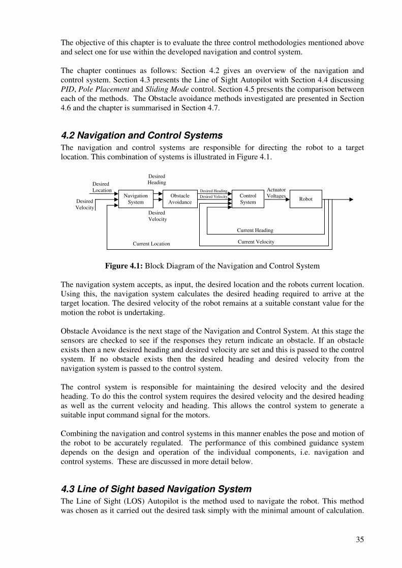
35
The objective of this chapter is to evaluate the three control methodologies mentioned above and select one for use within the developed navigation and control system. The chapter continues as follows: Section 4.2 gives an overview of the navigation and control system. Section 4.3 presents the Line of Sight Autopilot with Section 4.4 discussing PID, Pole Placement and Sliding Mode control. Section 4.5 presents the comparison between each of the methods. The Obstacle avoidance methods investigated are presented in Section 4.6 and the chapter is summarised in Section 4.7.
4.2 Navigation and Control Systems
The navigation and control systems are responsible for directing the robot to a target location. This combination of systems is illustrated in Figure 4.1.
Figure 4.1: Block Diagram of the Navigation and Control System
The navigation system accepts, as input, the desired location and the robots current location. Using this, the navigation system calculates the desired heading required to arrive at the target location. The desired velocity of the robot remains at a suitable constant value for the motion the robot is undertaking. Obstacle Avoidance is the next stage of the Navigation and Control System. At this stage the sensors are checked to see if the responses they return indicate an obstacle. If an obstacle exists then a new desired heading and desired velocity are set and this is passed to the control system. If no obstacle exists then the desired heading and desired velocity from the navigation system is passed to the control system. The control system is responsible for maintaining the desired velocity and the desired heading. To do this the control system requires the desired velocity and the desired heading as well as the current velocity and heading. This allows the control system to generate a suitable input command signal for the motors. Combining the navigation and control systems in this manner enables the pose and motion of the robot to be accurately regulated. The performance of this combined guidance system depends on the design and operation of the individual components, i.e. navigation and control systems. These are discussed in more detail below.
4.3 Line of Sight based Navigation System
The Line of Sight (LOS) Autopilot is the method used to navigate the robot. This method was chosen as it carried out the desired task simply with the minimal amount of calculation.
Control System
Current Heading
Current Velocity
Desired Velocity
Current Location
Navigation System
Actuator Voltages
Robot Obstacle
Avoidance
Desired Heading Desired Velocity
Desired Heading
Desired Velocity
Desired Location
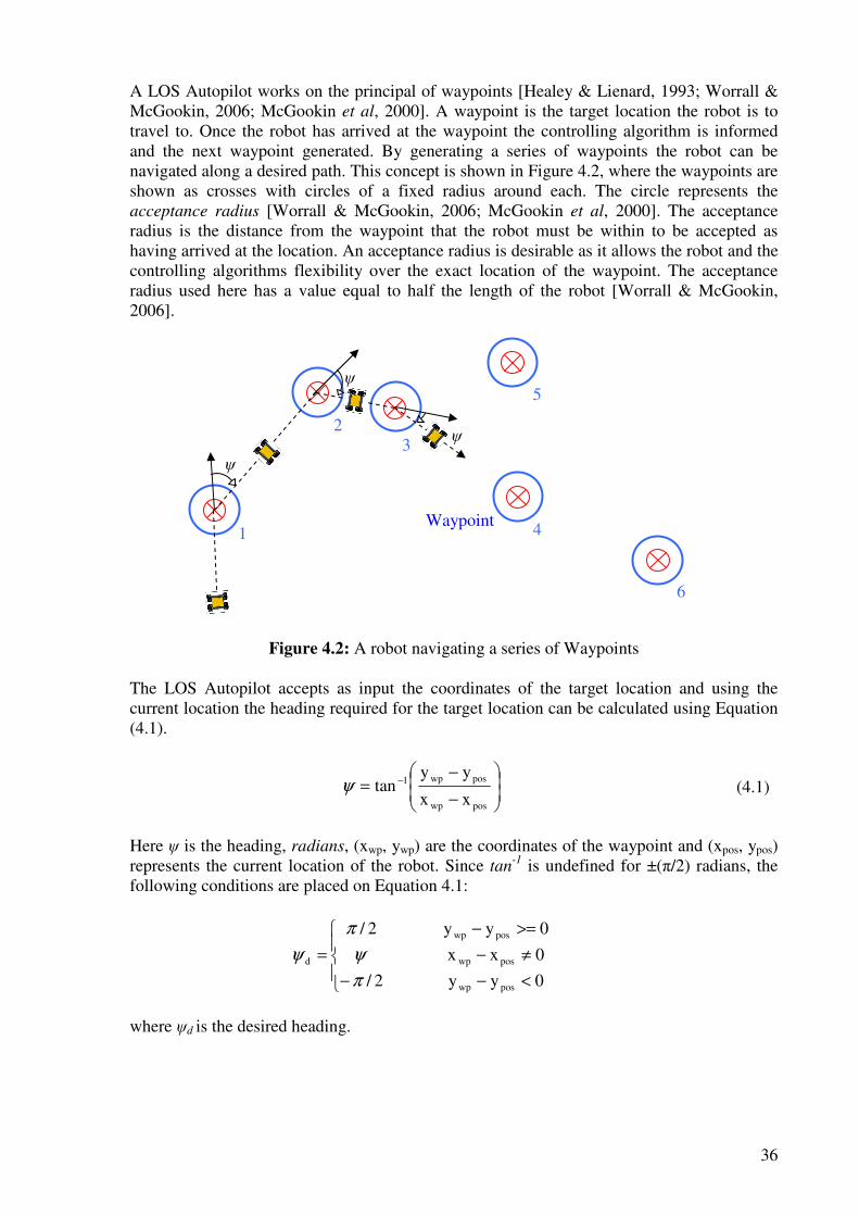
36
A LOS Autopilot works on the principal of waypoints [Healey & Lienard, 1993; Worrall & McGookin, 2006; McGookin et al, 2000]. A waypoint is the target location the robot is to travel to. Once the robot has arrived at the waypoint the controlling algorithm is informed and the next waypoint generated. By generating a series of waypoints the robot can be navigated along a desired path. This concept is shown in Figure 4.2, where the waypoints are shown as crosses with circles of a fixed radius around each. The circle represents the acceptance radius [Worrall & McGookin, 2006; McGookin et al, 2000]. The acceptance radius is the distance from the waypoint that the robot must be within to be accepted as having arrived at the location. An acceptance radius is desirable as it allows the robot and the controlling algorithms flexibility over the exact location of the waypoint. The acceptance radius used here has a value equal to half the length of the robot [Worrall & McGookin, 2006].
Figure 4.2: A robot navigating a series of Waypoints
The LOS Autopilot accepts as input the coordinates of the target location and using the current location the heading required for the target location can be calculated using Equation (4.1).
−
−= −
poswp
poswp1
xx
yytanψ (4.1)
Here ψ is the heading, radians, (xwp, ywp) are the coordinates of the waypoint and (xpos, ypos) represents the current location of the robot. Since tan
-1 is undefined for ±(π/2) radians, the following conditions are placed on Equation 4.1:
0yy
0xx
0yy
2/
2/
poswp
poswp
poswp
d
<−
≠−
>=−
−
=
π
ψ
π
ψ
where ψd is the desired heading.
1
2 3
4
5
6
Waypoint
ψ
ψ
ψ
37
4.4 Control System
As discussed, the control system is concerned with maintaining the desired velocity and the desired heading. In order to achieve this, a control methodology is implemented which is designed to generate suitable input command signals for the motors. The three control methodologies considered here are PID, Pole Placement and Sliding Mode. In this section the theory and implementation of each control methodology is discussed. Each control methodology was tested in a series of experiments which were designed to test various aspects of the controllers developed. The results achieved by each controller is presented.
4.4.1 Experiments
A series of experiments have been designed to test each controller. The experiments set the desired responses over a period of time, in this case 20 seconds. The experiments are designed to show if the model responds accurately, under the control of one of the controllers developed and how quickly the model responds to the input commands. Seven experiments have been developed and are described below.
• Experiment 1
A desired velocity for the full length of the experiment is the first experiment. This experiment shows if the controller is able to maintain a desired velocity.
• Experiment 2
The controller also needs to be able to maintain a desired heading. Experiment 2 sets a desired heading for the full length of time.
• Experiment 3
The previous two experiments aim to show the controller handling a desired constant value. The controller also needs to be able to handle changes in the desired value. Experiment 3 sets a desired velocity for 10 seconds then changes to a second value for the desired velocity for the next 10 seconds.
• Experiment 4
This experiment is designed to test the controller’s ability to handle a change in the desired heading. Experiment 4 sets a desired heading for 10 seconds then changes the desired heading to a second value for the next 10 seconds.
• Experiment 5
The next test is to see if the controller can handle repeated changes in the desired velocity. Experiment 5 changes the desired velocity between two values every 4 seconds.
• Experiment 6
As with the velocity, repeated changes in the desired heading are used to test the controller. Experiment 6 changes the desired heading between two values every 4 seconds.
• Experiment 7
The previous experiments have all tested the response from the controller when only one of the desired values has been changed. Experiment 7 changes the desired velocity between two values every 4 seconds and changes the desired heading, between two values 2 seconds after each change in the desired velocity. This
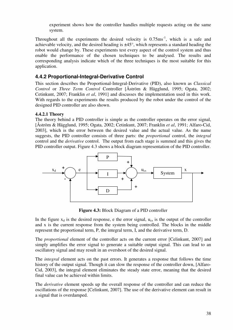
38
experiment shows how the controller handles multiple requests acting on the same system.
Throughout all the experiments the desired velocity is 0.75ms-1, which is a safe and achievable velocity, and the desired heading is ±45°, which represents a standard heading the robot would change by. These experiments test every aspect of the control system and thus enable the performance of the chosen techniques to be analysed. The results and corresponding analysis indicate which of the three techniques is the most suitable for this application.
4.4.2 Proportional-Integral-Derivative Control
This section describes the Proportional-Integral-Derivative (PID), also known as Classical
Control or Three Term Control Controller [Åström & Hägglund, 1995; Ogata, 2002; Cetinkunt, 2007; Franklin et al, 1991] and discusses the implementation used in this work. With regards to the experiments the results produced by the robot under the control of the designed PID controller are also shown.
4.4.2.1 Theory
The theory behind a PID controller is simple as the controller operates on the error signal, [Åström & Hägglund, 1995; Ogata, 2002; Cetinkunt, 2007; Franklin et al, 1991; Alfaro-Cid, 2003], which is the error between the desired value and the actual value. As the name suggests, the PID controller consists of three parts: the proportional control, the integral control and the derivative control. The output from each stage is summed and this gives the PID controller output. Figure 4.3 shows a block diagram representation of the PID controller.
Figure 4.3: Block Diagram of a PID controller
In the figure xd is the desired response, e the error signal, ucs is the output of the controller and x is the current response from the system being controlled. The blocks in the middle represent the proportional term, P, the integral term, I, and the derivative term, D.
The proportional element of the controller acts on the current error [Celinkunt, 2007] and simply amplifies the error signal to generate a suitable output signal. This can lead to an oscillatory signal and may result in an overshoot of the desired signal.
The integral element acts on the past errors. It generates a response that follows the time history of the output signal. Though it can slow the response of the controller down, [Alfaro-Cid, 2003], the integral element eliminates the steady state error, meaning that the desired final value can be achieved within limits.
The derivative element speeds up the overall response of the controller and can reduce the oscillations of the response [Celinkunt, 2007]. The use of the derivative element can result in a signal that is overdamped.
P
+
+
xd +
-
e ucs x I
D
System
+
39
The standard continuous time equation for a PID is:
∫ ++=t
0dt
)t(dedipcs .Kdt).t(e.K)t(e.K)t(u (4.2)
here ucs (t) is the output signal, e(t) is the error signal and Kp, Ki and Kd are the gains of the Proportional, Integral and Derivative elements respectively. Equation (4.2) can also be stated in a discrete time form, as shown in Equation (4.3) [Celinkunt, 2007; Åström & Hägglund, 1995]. The equation in the discrete time form is the method best used for implementing the PID controller on a computer or within a microcontroller.
t
)ee(.K)t(e.K)t(e.K)t(u 1tntn
dniinpncs∆
−++= − (4.3)
Where tn is the current time, tn-1 is the pervious time, ∆t is the time stepsize and ei(tn) is:
∑ ∆+= −
nt
on1nni t).t(e)t(e)t(e (4.4)
4.4.2.2 Tuning PID terms
The gains, Kp, Ki and Kd are constants that require to be tuned to an appropriate value. Tuning is the process of selecting the gains of a PID controller to give the required performance specifications [Ogata, 2002]. The tuning is designed to give the response that the user wants from the application. Different gain settings and different combinations of gain settings result in different responses. In the application considered here a fast response with no steady state error would be the desired response. No overshoot would also be desired as this will decrease the demands made on the actuators. It is possible to manually tune the gains for a PID controller [Ogata, 2002; Alfaro-Cid, 2003]. However, this can be an exhaustive process and may not lead to the optimal gain settings or even gains that give a near reasonable response. One method for tuning PID controllers that is often described alongside the PID controller is the Ziegler-Nichols method [Ziegler & Nichols, 1942; Åström & Hägglund, 1995; Ogata, 2002; Alfaro-Cid, 2003; Franklin et al, 1991]. The Ziegler-Nichols method uses information, namely the delay time, L, and the time constant, T, gained from the response of the model to a step input. These two parameters are then used to calculate the gains in the following way, Kp = 1.2(T/L), Ki = 2L and Kd = 0.5L [Ogata, 2002; Alfaro-Cid, 2003; Franklin et al, 1991]. Though this method gives values that can be used, it is accepted that the Ziegler-Nichols method gives more of an approximation of the values of the gains and that the gains calculated require fine tuning to give a better desired response [Ogata, 2002; Alfaro-Cid, 2003; Franklin et al, 1991]. Using the Ziegler-Nichols method achieved approximate values for the controller gains. The gains achieved were then slightly altered by hand to give a better response. 4.4.2.3 Integral Antiwindup
There can come a point in any real system, or properly modelled simulation, where the output from a controller is beyond the range of the actuator it is controlling. This results in the actuator becoming saturated. An example of this would be when the control circuit for a
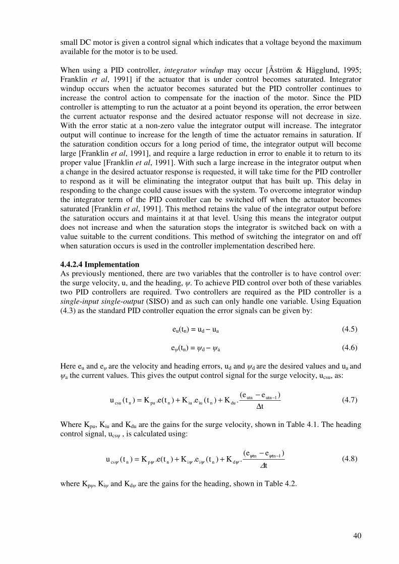
40
small DC motor is given a control signal which indicates that a voltage beyond the maximum available for the motor is to be used. When using a PID controller, integrator windup may occur [Åström & Hägglund, 1995; Franklin et al, 1991] if the actuator that is under control becomes saturated. Integrator windup occurs when the actuator becomes saturated but the PID controller continues to increase the control action to compensate for the inaction of the motor. Since the PID controller is attempting to run the actuator at a point beyond its operation, the error between the current actuator response and the desired actuator response will not decrease in size. With the error static at a non-zero value the integrator output will increase. The integrator output will continue to increase for the length of time the actuator remains in saturation. If the saturation condition occurs for a long period of time, the integrator output will become large [Franklin et al, 1991], and require a large reduction in error to enable it to return to its proper value [Franklin et al, 1991]. With such a large increase in the integrator output when a change in the desired actuator response is requested, it will take time for the PID controller to respond as it will be eliminating the integrator output that has built up. This delay in responding to the change could cause issues with the system. To overcome integrator windup the integrator term of the PID controller can be switched off when the actuator becomes saturated [Franklin et al, 1991]. This method retains the value of the integrator output before the saturation occurs and maintains it at that level. Using this means the integrator output does not increase and when the saturation stops the integrator is switched back on with a value suitable to the current conditions. This method of switching the integrator on and off when saturation occurs is used in the controller implementation described here. 4.4.2.4 Implementation
As previously mentioned, there are two variables that the controller is to have control over: the surge velocity, u, and the heading, ψ. To achieve PID control over both of these variables two PID controllers are required. Two controllers are required as the PID controller is a single-input single-output (SISO) and as such can only handle one variable. Using Equation (4.3) as the standard PID controller equation the error signals can be given by:
eu(tn) = ud − ua (4.5)
eψ(tn) = ψd − ψa (4.6) Here eu and eψ are the velocity and heading errors, ud and ψd are the desired values and ua and ψa the current values. This gives the output control signal for the surge velocity, ucsu, as:
t
)ee(.K)t(e.K)t(e.K)t(u 1utnutn
duniuiunpuncsu∆
−++= − (4.7)
Where Kpu, Kiu and Kdu are the gains for the surge velocity, shown in Table 4.1. The heading control signal, ucsψ , is calculated using:
t
)ee(.K)t(e.K)t(e.K)t(u 1tntn
dniinpncs∆
ψψ
ψψψψψ
−−++= (4.8)
where Kpψ, Kiψ and Kdψ are the gains for the heading, shown in Table 4.2.
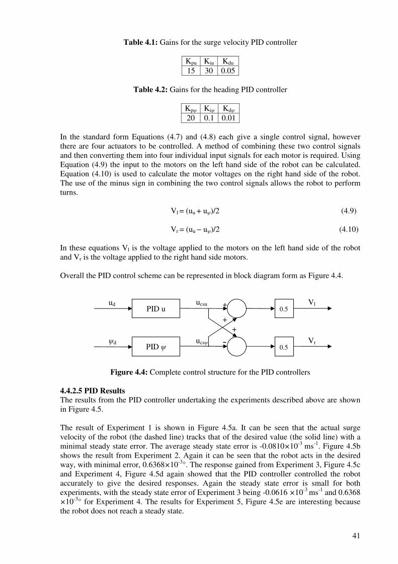
41
Table 4.1: Gains for the surge velocity PID controller
Kpu Kiu Kdu 15 30 0.05
Table 4.2: Gains for the heading PID controller
Kpψ Kiψ Kdψ 20 0.1 0.01
In the standard form Equations (4.7) and (4.8) each give a single control signal, however there are four actuators to be controlled. A method of combining these two control signals and then converting them into four individual input signals for each motor is required. Using Equation (4.9) the input to the motors on the left hand side of the robot can be calculated. Equation (4.10) is used to calculate the motor voltages on the right hand side of the robot. The use of the minus sign in combining the two control signals allows the robot to perform turns.
Vl = (uu + uψ)/2 (4.9)
Vr = (uu − uψ)/2 (4.10)
In these equations Vl is the voltage applied to the motors on the left hand side of the robot and Vr is the voltage applied to the right hand side motors. Overall the PID control scheme can be represented in block diagram form as Figure 4.4.
Figure 4.4: Complete control structure for the PID controllers
4.4.2.5 PID Results
The results from the PID controller undertaking the experiments described above are shown in Figure 4.5. The result of Experiment 1 is shown in Figure 4.5a. It can be seen that the actual surge velocity of the robot (the dashed line) tracks that of the desired value (the solid line) with a minimal steady state error. The average steady state error is -0.0810×10⁻³ ms-1. Figure 4.5b shows the result from Experiment 2. Again it can be seen that the robot acts in the desired way, with minimal error, 0.6368×10⁻³°. The response gained from Experiment 3, Figure 4.5c and Experiment 4, Figure 4.5d again showed that the PID controller controlled the robot accurately to give the desired responses. Again the steady state error is small for both experiments, with the steady state error of Experiment 3 being -0.0616 ×10⁻³ ms-1 and 0.6368
×10-3° for Experiment 4. The results for Experiment 5, Figure 4.5e are interesting because the robot does not reach a steady state.
ud 0.5
0.5 ψd
Vl
Vr
PID u
PID ψ
ucsu
ucsψ
+
+ +
-
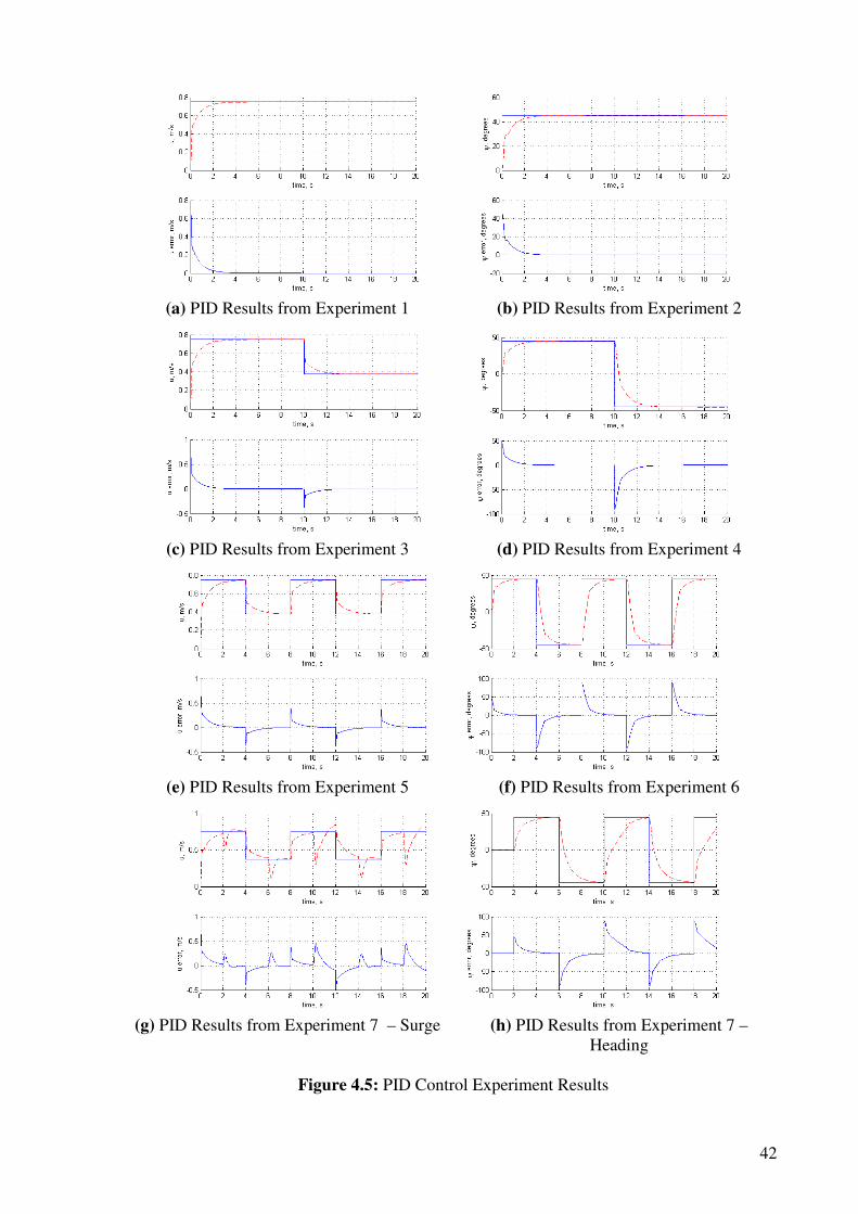
42
(a) PID Results from Experiment 1 (b) PID Results from Experiment 2
(c) PID Results from Experiment 3 (d) PID Results from Experiment 4
(e) PID Results from Experiment 5 (f) PID Results from Experiment 6
(g) PID Results from Experiment 7 – Surge (h) PID Results from Experiment 7 –
Heading
Figure 4.5: PID Control Experiment Results
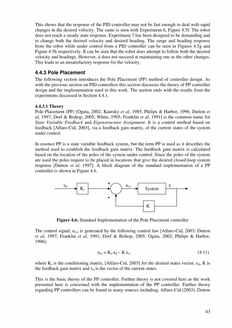
43
This shows that the response of the PID controller may not be fast enough to deal with rapid changes in the desired velocity. The same is seen with Experiment 6, Figure 4.5f. The robot does not reach a steady state response. Experiment 7 has been designed to be demanding and to change both the desired velocity and desired heading. The surge and heading response from the robot while under control from a PID controller can be seen in Figures 4.5g and Figure 4.5h respectively. It can be seen that the robot does attempt to follow both the desired velocity and headings. However, it does not succeed at maintaining one as the other changes. This leads to an unsatisfactory response for the velocity.
4.4.3 Pole Placement
The following section introduces the Pole Placement (PP) method of controller design. As with the previous section on PID controllers this section discusses the theory of PP controller design and the implementation used in this work. The section ends with the results from the experiments discussed in Section 4.4.1. 4.4.3.1 Theory
Pole Placement (PP) [Ogata, 2002; Kautsky et al, 1985; Philips & Harbor, 1996; Dutton et
al, 1997; Dorf & Bishop, 2005; White, 1995; Franklin et al, 1991] is the common name for State Variable Feedback and Eigenstructure Assignment. It is a control method based on feedback [Alfaro-Cid, 2003], via a feedback gain matrix, of the current states of the system under control. In essence PP is a state variable feedback system, but the term PP is used as it describes the method used to establish the feedback gain matrix. The feedback gain matrix is calculated based on the location of the poles of the system under control. Since the poles of the system are used the poles require to be placed in locations that give the desired closed-loop system response [Dutton et al, 1997]. A block diagram of the standard implementation of a PP controller is shown in Figure 4.6.
Figure 4.6: Standard Implementation of the Pole Placement controller
The control signal, ucs, is generated by the following control law [Alfaro-Cid, 2003; Dutton et al, 1997; Franklin et al, 1991; Dorf & Bishop, 2005; Ogata, 2002; Philips & Harbor, 1996]:
ucs = Kr.xd − K.xa (4.11) where Kr is the conditioning matrix, [Alfaro-Cid, 2003] for the desired states vector, xd, K is the feedback gain matrix and xa is the vector of the current states. This is the basic theory of the PP controller. Further theory is not covered here as the work presented here is concerned with the implementation of the PP controller. Further theory regarding PP controllers can be found in many sources including; Alfaro-Cid (2003), Dutton
+
-
xd ucs x System
Kr
K
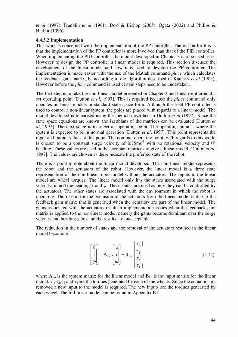
44
et al (1997), Franklin et al (1991), Dorf & Bishop (2005), Ogata (2002) and Philips & Harbor (1996).
4.4.3.2 Implementation
This work is concerned with the implementation of the PP controller. The reason for this is that the implementation of the PP controller is more involved than that of the PID controller. When implementing the PID controller the model developed in Chapter 3 can be used as is. However to design the PP controller a linear model is required. This section discuses the development of the linear model and how it is used to develop the PP controller. The implementation is made easier with the use of the Matlab command place which calculates the feedback gain matrix, K, according to the algorithm described in Kautsky et al (1985). However before the place command is used certain steps need to be undertaken.
The first step is to take the non-linear model presented in Chapter 3 and linearise it around a set operating point [Dutton et al, 1997]. This is required because the place command only operates on linear models in standard state space form. Although the final PP controller is used to control a non-linear system, the poles are placed with regards to a linear model. The model developed is linearised using the method described in Dutton et al (1997). Since the state space equations are known, the Jacobians of the matrices can be evaluated [Dutton et
al, 1997]. The next stage is to select an operating point. The operating point is where the system is expected to be in normal operation [Dutton et al, 1997]. This point represents the input and output values at this point. The nominal operating point, with regards to this work, is chosen to be a constant surge velocity of 0.75ms-1 with no rotational velocity and 0° heading. These values are used in the Jacobian matrices to give a linear model [Dutton et al, 1997]. The values are chosen as these indicate the preferred state of the robot.
There is a point to note about the linear model developed. The non-linear model represents the robot and the actuators of the robot. However, the linear model is a three state representation of the non-linear robot model without the actuators. The inputs to the linear model are wheel torques. The linear model only has the states associated with the surge velocity, u, and the heading, r and ψ. These states are used as only they can be controlled by the actuators. The other states are associated with the environment in which the robot is operating. The reason for the exclusion of the actuators from the linear model is due to the feedback gain matrix that is generated when the actuators are part of the linear model. The gains associated with the actuators result in implementation issues when the feedback gain matrix is applied to the non-linear model, namely the gains became dominant over the surge velocity and heading gains and the results are unacceptable.
The reduction in the number of states and the removal of the actuators resulted in the linear model becoming:
+
=
4
3
2
1
LinLin .Br
u
.Ar
u
τ
τ
τ
τ
ψψ&&
&
(4.12)
where Alin is the system matrix for the linear model and Blin is the input matrix for the linear model. τ1, τ2, τ3 and τ4 are the torques generated by each of the wheels. Since the actuators are removed a new input to the model is required. The new inputs are the torques generated by each wheel. The full linear model can be found in Appendix B1.
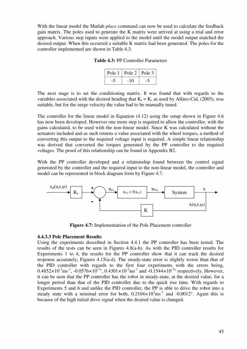
45
With the linear model the Matlab place command can now be used to calculate the feedback gain matrix. The poles used to generate the K matrix were arrived at using a trial and error approach. Various step inputs were applied to the model until the model output matched the desired output. When this occurred a suitable K matrix had been generated. The poles for the controller implemented are shown in Table 4.3.
Table 4.3: PP Controller Parameters
Pole 1 Pole 2 Pole 3
-5 -10 -5 The next stage is to set the conditioning matrix. It was found that with regards to the variables associated with the desired heading that Kr = K, as used by Alfaro-Cid, (2003), was suitable, but for the surge velocity the value had to be manually tuned. The controller for the linear model in Equation (4.12) using the setup shown in Figure 4.6 has now been developed. However one more step is required to allow the controller, with the gains calculated, to be used with the non-linear model. Since K was calculated without the actuators included and as such returns a value associated with the wheel torques, a method of converting this output to the required voltage input is required. A simple linear relationship was derived that converted the torques generated by the PP controller to the required voltages. The proof of this relationship can be found in Appendix B2. With the PP controller developed and a relationship found between the control signal generated by the controller and the required input to the non-linear model, the controller and model can be represented in block diagram form by Figure 4.7.
Figure 4.7: Implementation of the Pole Placement controller 4.4.3.3 Pole Placement Results
Using the experiments described in Section 4.4.1 the PP controller has been tested. The results of the tests can be seen in Figures 4.8(a-h). As with the PID controller results for Experiments 1 to 4, the results for the PP controller show that it can track the desired response accurately, Figures 4.15(a-d). The steady-state error is slightly worse than that of the PID controller with regards to the first four experiments with the errors being, 0.4852×10⁻³ms-1, -0.0576×10⁻³°, 0.4301×10⁻³ms-1 and -0.1544×10⁻³° respectively. However, it can be seen that the PP controller has the robot in steady-state, at the desired value, for a longer period than that of the PID controller due to the quick rise time. With regards to Experiments 5 and 6 and unlike the PID controller, the PP is able to drive the robot into a steady state with a minimal error for both, 0.2104×10³ms-1 and -0.0012°. Again this is because of the high initial drive signal when the desired value is changed.
+
-
xd(u,r,ψ) ucs x System
Kr
K
uVa = f(ucs)
uVa
x(u,r,ψ)
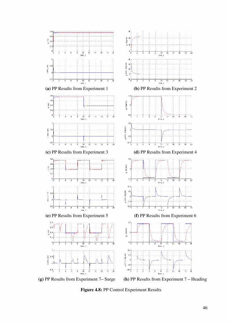
46
(a) PP Results from Experiment 1 (b) PP Results from Experiment 2
(c) PP Results from Experiment 3 (d) PP Results from Experiment 4
(e) PP Results from Experiment 5 (f) PP Results from Experiment 6
(g) PP Results from Experiment 7– Surge (h) PP Results from Experiment 7 – Heading
Figure 4.8: PP Control Experiment Results
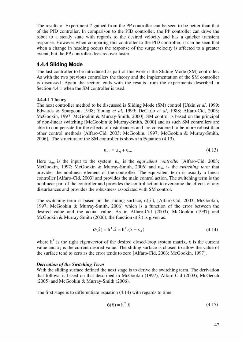
47
The results of Experiment 7 gained from the PP controller can be seen to be better than that of the PID controller. In comparison to the PID controller, the PP controller can drive the robot to a steady state with regards to the desired velocity and has a quicker transient response. However when comparing this controller to the PID controller, it can be seen that when a change in heading occurs the response of the surge velocity is affected to a greater extent, but the PP controller does recover faster.
4.4.4 Sliding Mode
The last controller to be introduced as part of this work is the Sliding Mode (SM) controller. As with the two previous controllers the theory and the implementation of the SM controller is discussed. Again the section ends with the results from the experiments described in Section 4.4.1 when the SM controller is used. 4.4.4.1 Theory
The next controller method to be discussed is Sliding Mode (SM) control [Utkin et al, 1999; Edwards & Spurgeon, 1998; Young et al, 1999; DeCarlo et al, 1988; Alfaro-Cid, 2003; McGookin, 1997; McGookin & Murray-Smith, 2000]. SM control is based on the principal of non-linear switching [McGookin & Murray-Smith, 2000] and as such SM controllers are able to compensate for the effects of disturbances and are considered to be more robust than other control methods [Alfaro-Cid, 2003; McGookin, 1997; McGookin & Murray-Smith, 2006]. The structure of the SM controller is shown in Equation (4.13).
usm = ueq + usw (4.13) Here usm is the input to the system, ueq is the equivalent controller [Alfaro-Cid, 2003; McGookin, 1997; McGookin & Murray-Smith, 2006] and usw is the switching term that provides the nonlinear element of the controller. The equivalent term is usually a linear controller [Alfaro-Cid, 2003] and provides the main control action. The switching term is the nonlinear part of the controller and provides the control action to overcome the effects of any disturbances and provides the robustness associated with SM control. The switching term is based on the sliding surface, σ( x ), [Alfaro-Cid, 2003; McGookin, 1997; McGookin & Murray-Smith, 2006] which is a function of the error between the desired value and the actual value. As in Alfaro-Cid (2003), McGookin (1997) and McGookin & Murray-Smith (2006), the function σ( x ) is given as:
)xx.(hx.h)x( dTT −==σ (4.14)
where hT is the right eigenvector of the desired closed-loop system matrix, x is the current value and xd is the current desired value. The sliding surface is chosen to allow the value of the surface tend to zero as the error tends to zero [Alfaro-Cid, 2003; McGookin, 1997].
Derivation of the Switching Term With the sliding surface defined the next stage is to derive the switching term. The derivation that follows is based on that described in McGookin (1997), Alfaro-Cid (2003), McGeoch (2005) and McGookin & Murray-Smith (2006). The first stage is to differentiate Equation (4.14) with regards to time:
x.h)x( T && =σ (4.15)
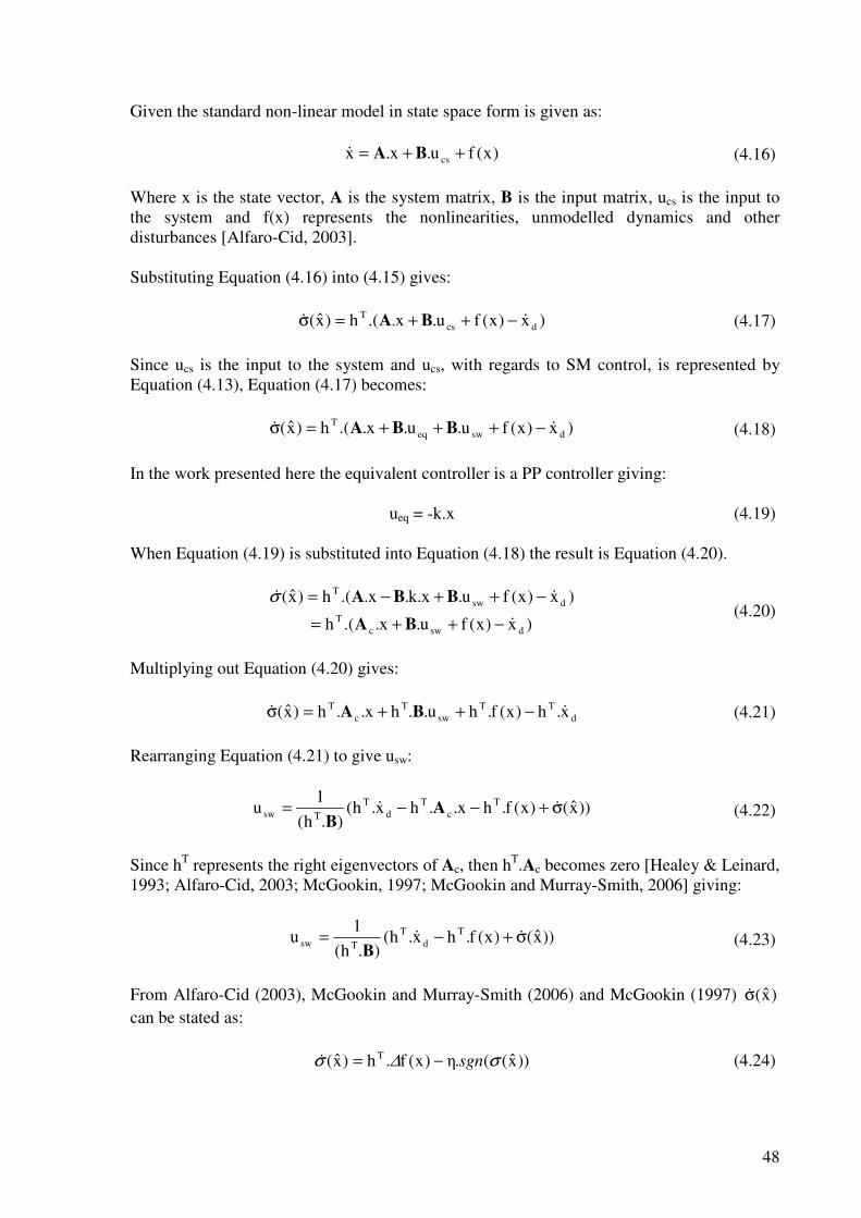
48
Given the standard non-linear model in state space form is given as:
)x(fu.x.x cs ++= BA& (4.16)
Where x is the state vector, A is the system matrix, B is the input matrix, ucs is the input to the system and f(x) represents the nonlinearities, unmodelled dynamics and other disturbances [Alfaro-Cid, 2003]. Substituting Equation (4.16) into (4.15) gives:
)x)x(fu.x..(h)x( dcsT
&& −++=σ BA (4.17)
Since ucs is the input to the system and ucs, with regards to SM control, is represented by Equation (4.13), Equation (4.17) becomes:
)x)x(fu.u.x..(h)x( dsweqT
&& −+++=σ BBA (4.18)
In the work presented here the equivalent controller is a PP controller giving:
ueq = -k.x (4.19) When Equation (4.19) is substituted into Equation (4.18) the result is Equation (4.20).
)x)x(fu.x.k.x..(h)x( dswT
&& −++−= BBAσ
)x)x(fu.x..(h dswcT
&−++= BA (4.20)
Multiplying out Equation (4.20) gives:
dTT
swT
cT x.h)x(f.hu..hx..h)x( && −++=σ BA (4.21)
Rearranging Equation (4.21) to give usw:
))x()x(f.hx..hx.h().h(
1u T
cT
dT
Tsw σ+−−= && AB
(4.22)
Since hT represents the right eigenvectors of Ac, then hT.Ac becomes zero [Healey & Leinard, 1993; Alfaro-Cid, 2003; McGookin, 1997; McGookin and Murray-Smith, 2006] giving:
))x()x(f.hx.h().h(
1u T
dT
Tsw σ+−= &&B
(4.23)
From Alfaro-Cid (2003), McGookin and Murray-Smith (2006) and McGookin (1997) )x(σ& can be stated as:
))x((.η)x(f.h)x( T σ∆σ sgn−=& (4.24)
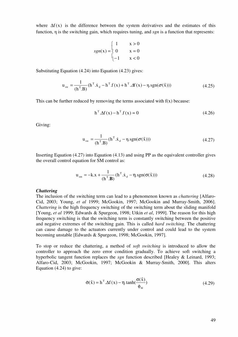
49
where )x(f∆ is the difference between the system derivatives and the estimates of this function, η is the switching gain, which requires tuning, and sgn is a function that represents:
0x
0x
0x
1
0
1
)x(
<
=
>
−
=sgn
Substituting Equation (4.24) into Equation (4.23) gives:
)))x(sgn(.η)x(f.h)x(f.hx.h()B.h(
1u TT
dT
Tsw σ∆ −+−= & (4.25)
This can be further reduced by removing the terms associated with f(x) because:
0)x(f.h)x(f.h TT ≈−∆ (4.26)
Giving:
)))x(sgn(.ηx.h()B.h(
1u d
TTsw σ−= & (4.27)
Inserting Equation (4.27) into Equation (4.13) and using PP as the equivalent controller gives the overall control equation for SM control as:
)))x(sgn(.x.h().h(
1x.ku d
TTsm ση−+−= &
B (4.28)
Chattering The inclusion of the switching term can lead to a phenomenon known as chattering [Alfaro-Cid, 2003; Young, et al 1999; McGookin, 1997; McGookin and Murray-Smith, 2006]. Chattering is the high frequency switching of the switching term about the sliding manifold [Young, et al 1999; Edwards & Spurgeon, 1998; Utkin et al, 1999]. The reason for this high frequency switching is that the switching term is constantly switching between the positive and negative extremes of the switching gain. This is called hard switching. The chattering can cause damage to the actuators currently under control and could lead to the system becoming unstable [Edwards & Spurgeon, 1998; McGookin, 1997]. To stop or reduce the chattering, a method of soft switching is introduced to allow the controller to approach the zero error condition gradually. To achieve soft switching a hyperbolic tangent function replaces the sgn function described [Healey & Leinard, 1993; Alfaro-Cid, 2003; McGookin, 1997; McGookin & Murray-Smith, 2000]. This alters Equation (4.24) to give:
))x(
tanh(.)x(f.h)x(bl
T
φ
ση−∆=σ& (4.29)
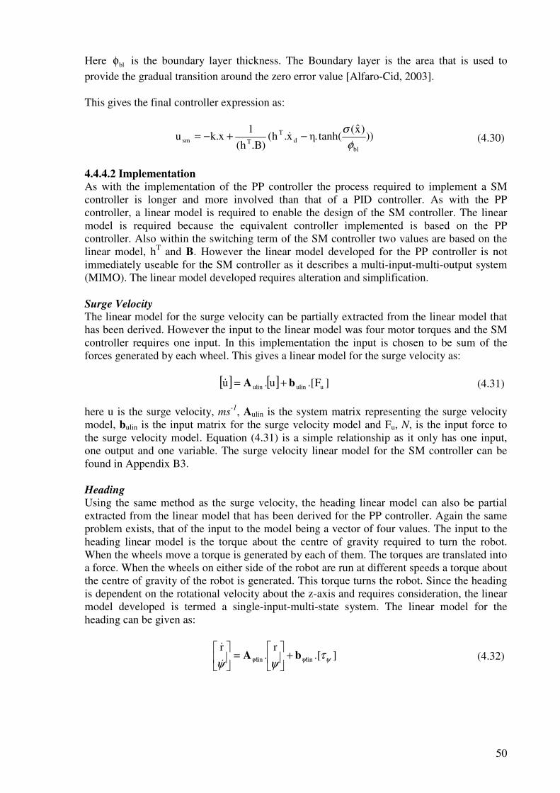
50
Here blφ is the boundary layer thickness. The Boundary layer is the area that is used to provide the gradual transition around the zero error value [Alfaro-Cid, 2003]. This gives the final controller expression as:
)))x(
tanh(.ηx.h()B.h(
1x.ku
bld
TTsm
φ
σ−+−= & (4.30)
4.4.4.2 Implementation
As with the implementation of the PP controller the process required to implement a SM controller is longer and more involved than that of a PID controller. As with the PP controller, a linear model is required to enable the design of the SM controller. The linear model is required because the equivalent controller implemented is based on the PP controller. Also within the switching term of the SM controller two values are based on the linear model, hT and B. However the linear model developed for the PP controller is not immediately useable for the SM controller as it describes a multi-input-multi-output system (MIMO). The linear model developed requires alteration and simplification. Surge Velocity The linear model for the surge velocity can be partially extracted from the linear model that has been derived. However the input to the linear model was four motor torques and the SM controller requires one input. In this implementation the input is chosen to be sum of the forces generated by each wheel. This gives a linear model for the surge velocity as:
[ ] [ ] ]F.[u.u uulinulin bA +=& (4.31)
here u is the surge velocity, ms-1, Aulin is the system matrix representing the surge velocity
model, bulin is the input matrix for the surge velocity model and Fu, N, is the input force to the surge velocity model. Equation (4.31) is a simple relationship as it only has one input, one output and one variable. The surge velocity linear model for the SM controller can be found in Appendix B3. Heading Using the same method as the surge velocity, the heading linear model can also be partial extracted from the linear model that has been derived for the PP controller. Again the same problem exists, that of the input to the model being a vector of four values. The input to the heading linear model is the torque about the centre of gravity required to turn the robot. When the wheels move a torque is generated by each of them. The torques are translated into a force. When the wheels on either side of the robot are run at different speeds a torque about the centre of gravity of the robot is generated. This torque turns the robot. Since the heading is dependent on the rotational velocity about the z-axis and requires consideration, the linear model developed is termed a single-input-multi-state system. The linear model for the heading can be given as:
].[r
.r
linlin ψψψ τψψ
bA +
=
&
& (4.32)
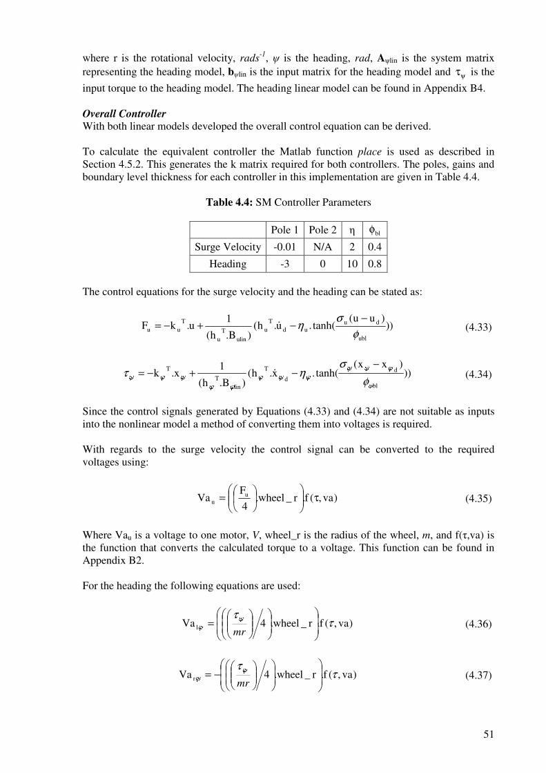
51
where r is the rotational velocity, rads-1, ψ is the heading, rad, Aψlin is the system matrix
representing the heading model, bψlin is the input matrix for the heading model and ψτ is the
input torque to the heading model. The heading linear model can be found in Appendix B4. Overall Controller With both linear models developed the overall control equation can be derived. To calculate the equivalent controller the Matlab function place is used as described in Section 4.5.2. This generates the k matrix required for both controllers. The poles, gains and boundary level thickness for each controller in this implementation are given in Table 4.4.
Table 4.4: SM Controller Parameters
Pole 1 Pole 2 η blφ
Surge Velocity -0.01 N/A 2 0.4
Heading -3 0 10 0.8 The control equations for the surge velocity and the heading can be stated as:
)))uu(
tanh(.u.h()B.h(
1u.kF
ubl
duud
Tu
ulinT
u
Tuu
φ
ση
−−+−= & (4.33)
)))xx(
tanh(.x.h()B.h(
1x.k
bl
d
d
T
linT
T ψ ψψψψψψψψψψψφ
σητ
−−+−= & (4.34)
Since the control signals generated by Equations (4.33) and (4.34) are not suitable as inputs into the nonlinear model a method of converting them into voltages is required. With regards to the surge velocity the control signal can be converted to the required voltages using:
)va,(f.r_wheel.4
FVa u
u τ
= (4.35)
Where Vau is a voltage to one motor, V, wheel_r is the radius of the wheel, m, and f(τ,va) is the function that converts the calculated torque to a voltage. This function can be found in Appendix B2. For the heading the following equations are used:
)va,(f.r_wheel.4Va l ττ
=
mr
ψψ (4.36)
)va,(f.r_wheel.4Va r ττ
−=
mr
ψψ (4.37)
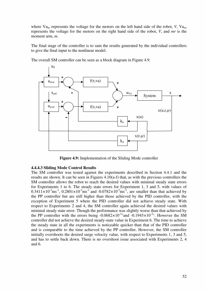
52
where Valψ represents the voltage for the motors on the left hand side of the robot, V, Varψ represents the voltage for the motors on the right hand side of the robot, V, and mr is the moment arm, m. The final stage of the controller is to sum the results generated by the individual controllers to give the final input to the nonlinear model. The overall SM controller can be seen as a block diagram in Figure 4.9.
Figure 4.9: Implementation of the Sliding Mode controller
4.4.4.3 Sliding Mode Control Results
The SM controller was tested against the experiments described in Section 4.4.1 and the results are shown. It can be seen in Figures 4.10(a-f) that, as with the previous controllers the SM controller allows the robot to reach the desired values with minimal steady state errors for Experiments 1 to 6. The steady state errors for Experiment 1, 3 and 5, with values of 0.3411×10⁻³ms-1, 0.2801×10⁻³ms-1 and -0.0782×10⁻³ms-1, are smaller than that achieved by the PP controller but are still higher than those achieved by the PID controller, with the exception of Experiment 5 where the PID controller did not achieve steady state. With respect to Experiments 2 and 4, the SM controller again achieved the desired values with minimal steady state error. Though the performance was slightly worse than that achieved by the PP controller with the errors being -0.0682×10⁻³°and -0.1945×10⁻³°. However the SM controller did not achieve the desired steady-state value in Experiment 6. The time to achieve the steady state in all the experiments is noticeable quicker than that of the PID controller and is comparable to the time achieved by the PP controller. However, the SM controller initially overshoots the desired surge velocity value, with respect to Experiments 1, 3 and 5, and has to settle back down. There is no overshoot issue associated with Experiments 2, 4 and 6.
x System
uusw
ku
f(τ,va)
uVa
x(u,r,ψ)
kψ
f(τ,va)
+
+ uψsw
ud
xψd
x(u)
x(r,ψ)
+
+
-
-
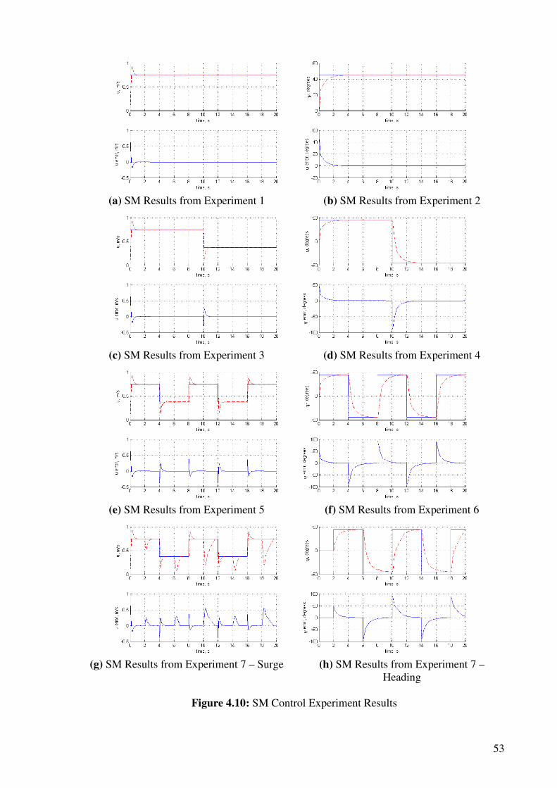
53
(a) SM Results from Experiment 1 (b) SM Results from Experiment 2
(c) SM Results from Experiment 3 (d) SM Results from Experiment 4
(e) SM Results from Experiment 5 (f) SM Results from Experiment 6
(g) SM Results from Experiment 7 – Surge (h) SM Results from Experiment 7 –
Heading
Figure 4.10: SM Control Experiment Results
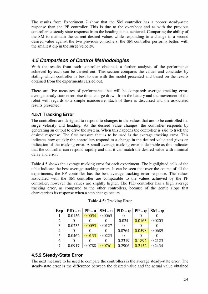
54
The results from Experiment 7 show that the SM controller has a poorer steady-state response than the PP controller. This is due to the overshoot and as with the previous controllers a steady state response from the heading is not achieved. Comparing the ability of the SM to maintain the current desired values while responding to a change in a second desired value against the two previous controllers, the SM controller performs better, with the smallest dip in the surge velocity.
4.5 Comparison of Control Methodologies
With the results from each controller obtained, a further analysis of the performance achieved by each can be carried out. This section compares the values and concludes by stating which controller is best to use with the model presented and based on the results obtained from the experiments carried out. There are five measures of performance that will be compared: average tracking error, average steady state error, rise time, charge drawn from the battery and the movement of the robot with regards to a simple manoeuvre. Each of these is discussed and the associated results presented.
4.5.1 Tracking Error
The controllers are designed to respond to changes in the values that are to be controlled i.e. surge velocity and heading. As the desired value changes, the controller responds by generating an output to drive the system. When this happens the controller is said to track the desired response. The first measure that is to be used is the average tracking error. This indicates how quickly the controllers respond to a change in the desired value and gives an indication of the tracking error. A small average tracking error is desirable as this indicates that the controller can respond rapidly and that it can match the desired value with minimal delay and error. Table 4.5 shows the average tracking error for each experiment. The highlighted cells of the table indicate the best average tracking errors. It can be seen that over the course of all the experiments, the PP controller has the best average tracking error response. The values associated with the SM controller are comparable to the values achieved by the PP controller, however the values are slightly higher. The PID controller has a high average tracking error, as compared to the other controllers, because of the gentle slope that characterises its response when a step change occurs.
Table 4.5: Tracking Error
Exp PID – u PP – u SM – u PID – ψ PP – ψ SM – ψ
1 0.0156 0.0054 0.0065 0 0 0 2 0 0 0 0.024 0.0163 0.0203 3 0.0235 0.0093 0.0127 0 0 0 4 0 0 0 0.0764 0.0598 0.0689 5 0.0462 0.0133 0.0223 0 0 0 6 0 0 0 0.2319 0.1892 0.2123 7 0.0917 0.0788 0.0761 0.2906 0.2152 0.2434
4.5.2 Steady-State Error
The next measure to be used to compare the controllers is the average steady-state error. The steady-state error is the difference between the desired value and the actual value obtained
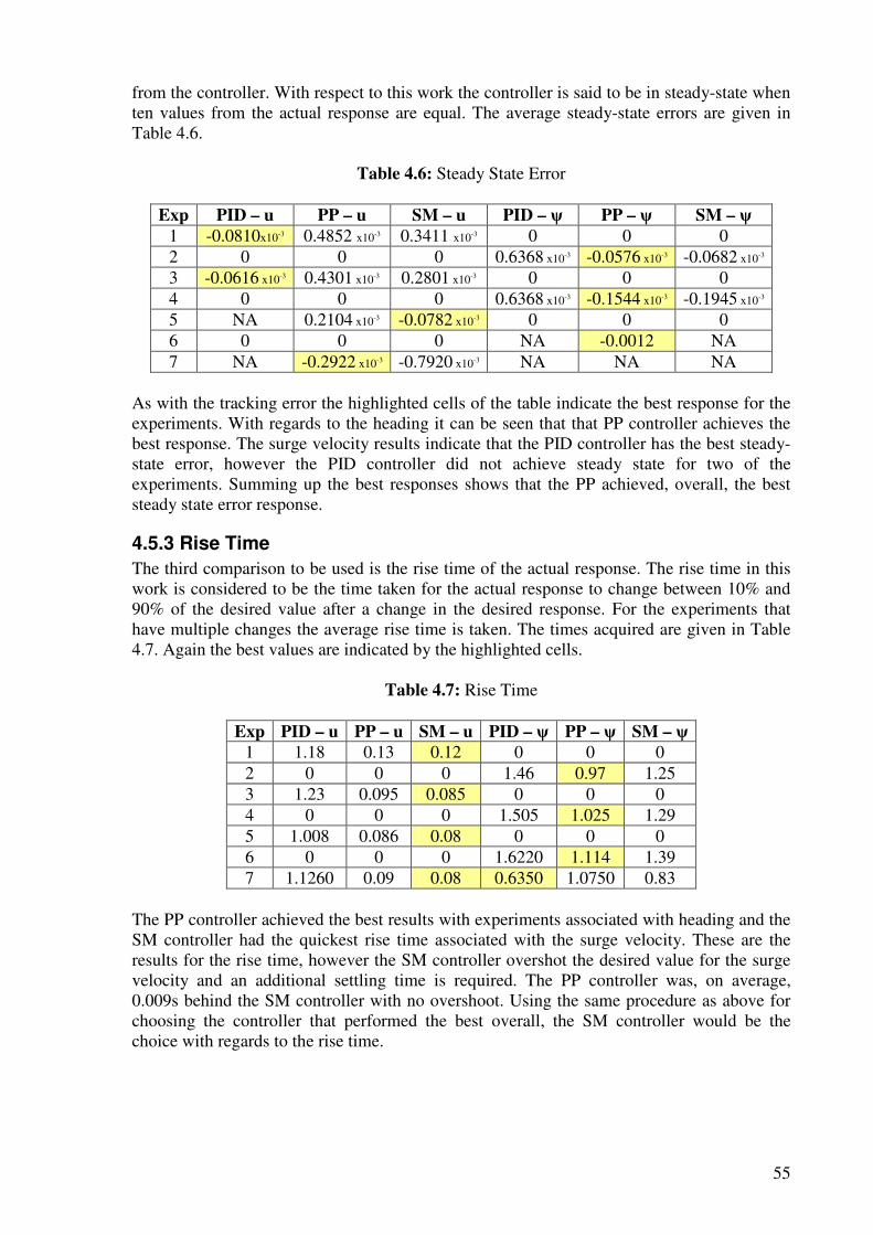
55
from the controller. With respect to this work the controller is said to be in steady-state when ten values from the actual response are equal. The average steady-state errors are given in Table 4.6.
Table 4.6: Steady State Error
Exp PID – u PP – u SM – u PID – ψ PP – ψ SM – ψ
1 -0.0810x10⁻³ 0.4852 x10⁻³ 0.3411 x10⁻³ 0 0 0 2 0 0 0 0.6368 x10⁻³ -0.0576 x10⁻³ -0.0682 x10⁻³ 3 -0.0616 x10⁻³ 0.4301 x10⁻³ 0.2801 x10⁻³ 0 0 0 4 0 0 0 0.6368 x10⁻³ -0.1544 x10⁻³ -0.1945 x10⁻³ 5 NA 0.2104 x10⁻³ -0.0782 x10⁻³ 0 0 0 6 0 0 0 NA -0.0012 NA 7 NA -0.2922 x10⁻³ -0.7920 x10⁻³ NA NA NA
As with the tracking error the highlighted cells of the table indicate the best response for the experiments. With regards to the heading it can be seen that that PP controller achieves the best response. The surge velocity results indicate that the PID controller has the best steady-state error, however the PID controller did not achieve steady state for two of the experiments. Summing up the best responses shows that the PP achieved, overall, the best steady state error response.
4.5.3 Rise Time
The third comparison to be used is the rise time of the actual response. The rise time in this work is considered to be the time taken for the actual response to change between 10% and 90% of the desired value after a change in the desired response. For the experiments that have multiple changes the average rise time is taken. The times acquired are given in Table 4.7. Again the best values are indicated by the highlighted cells.
Table 4.7: Rise Time
Exp PID – u PP – u SM – u PID – ψ PP – ψ SM – ψ
1 1.18 0.13 0.12 0 0 0 2 0 0 0 1.46 0.97 1.25 3 1.23 0.095 0.085 0 0 0 4 0 0 0 1.505 1.025 1.29 5 1.008 0.086 0.08 0 0 0 6 0 0 0 1.6220 1.114 1.39 7 1.1260 0.09 0.08 0.6350 1.0750 0.83
The PP controller achieved the best results with experiments associated with heading and the SM controller had the quickest rise time associated with the surge velocity. These are the results for the rise time, however the SM controller overshot the desired value for the surge velocity and an additional settling time is required. The PP controller was, on average, 0.009s behind the SM controller with no overshoot. Using the same procedure as above for choosing the controller that performed the best overall, the SM controller would be the choice with regards to the rise time.
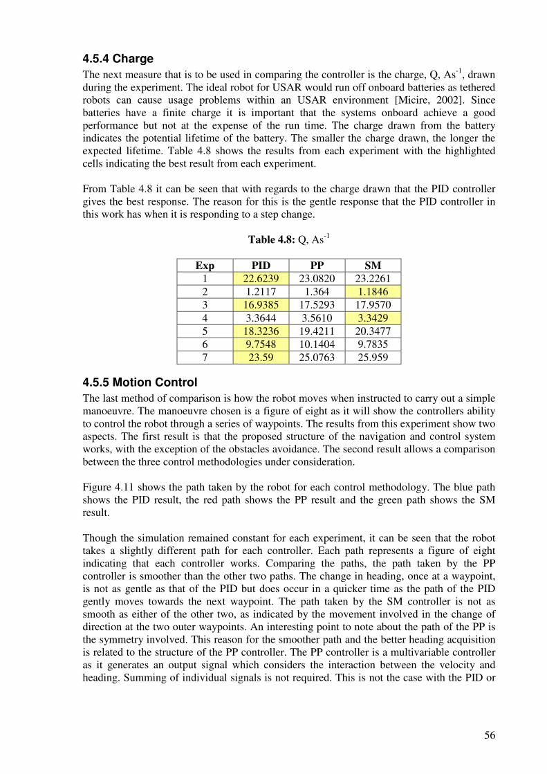
56
4.5.4 Charge
The next measure that is to be used in comparing the controller is the charge, Q, As-1, drawn during the experiment. The ideal robot for USAR would run off onboard batteries as tethered robots can cause usage problems within an USAR environment [Micire, 2002]. Since batteries have a finite charge it is important that the systems onboard achieve a good performance but not at the expense of the run time. The charge drawn from the battery indicates the potential lifetime of the battery. The smaller the charge drawn, the longer the expected lifetime. Table 4.8 shows the results from each experiment with the highlighted cells indicating the best result from each experiment. From Table 4.8 it can be seen that with regards to the charge drawn that the PID controller gives the best response. The reason for this is the gentle response that the PID controller in this work has when it is responding to a step change.
Table 4.8: Q, As-1
Exp PID PP SM
1 22.6239 23.0820 23.2261 2 1.2117 1.364 1.1846 3 16.9385 17.5293 17.9570 4 3.3644 3.5610 3.3429 5 18.3236 19.4211 20.3477 6 9.7548 10.1404 9.7835 7 23.59 25.0763 25.959
4.5.5 Motion Control
The last method of comparison is how the robot moves when instructed to carry out a simple manoeuvre. The manoeuvre chosen is a figure of eight as it will show the controllers ability to control the robot through a series of waypoints. The results from this experiment show two aspects. The first result is that the proposed structure of the navigation and control system works, with the exception of the obstacles avoidance. The second result allows a comparison between the three control methodologies under consideration. Figure 4.11 shows the path taken by the robot for each control methodology. The blue path shows the PID result, the red path shows the PP result and the green path shows the SM result. Though the simulation remained constant for each experiment, it can be seen that the robot takes a slightly different path for each controller. Each path represents a figure of eight indicating that each controller works. Comparing the paths, the path taken by the PP controller is smoother than the other two paths. The change in heading, once at a waypoint, is not as gentle as that of the PID but does occur in a quicker time as the path of the PID gently moves towards the next waypoint. The path taken by the SM controller is not as smooth as either of the other two, as indicated by the movement involved in the change of direction at the two outer waypoints. An interesting point to note about the path of the PP is the symmetry involved. This reason for the smoother path and the better heading acquisition is related to the structure of the PP controller. The PP controller is a multivariable controller as it generates an output signal which considers the interaction between the velocity and heading. Summing of individual signals is not required. This is not the case with the PID or
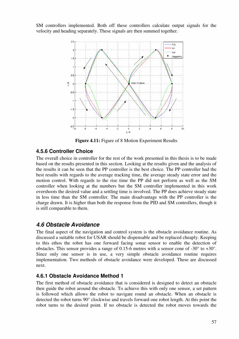
57
SM controllers implemented. Both off these controllers calculate output signals for the velocity and heading separately. These signals are then summed together.
Figure 4.11: Figure of 8 Motion Experiment Results
4.5.6 Controller Choice
The overall choice in controller for the rest of the work presented in this thesis is to be made based on the results presented in this section. Looking at the results given and the analysis of the results it can be seen that the PP controller is the best choice. The PP controller had the best results with regards to the average tracking time, the average steady state error and the motion control. With regards to the rise time the PP did not perform as well as the SM controller when looking at the numbers but the SM controller implemented in this work overshoots the desired value and a settling time is involved. The PP does achieve steady state in less time than the SM controller. The main disadvantage with the PP controller is the charge drawn. It is higher than both the response from the PID and SM controllers, though it is still comparable to them.
4.6 Obstacle Avoidance
The final aspect of the navigation and control system is the obstacle avoidance routine. As discussed a suitable robot for USAR should be dispensable and be replaced cheaply. Keeping to this ethos the robot has one forward facing sonar sensor to enable the detection of obstacles. This sensor provides a range of 0.15-6 metres with a sensor cone of -30° to +30°. Since only one sensor is in use, a very simple obstacle avoidance routine requires implementation. Two methods of obstacle avoidance were developed. These are discussed next.
4.6.1 Obstacle Avoidance Method 1
The first method of obstacle avoidance that is considered is designed to detect an obstacle then guide the robot around the obstacle. To achieve this with only one sensor, a set pattern is followed which allows the robot to navigate round an obstacle. When an obstacle is detected the robot turns 90° clockwise and travels forward one robot length. At this point the robot turns to the desired point. If no obstacle is detected the robot moves towards the
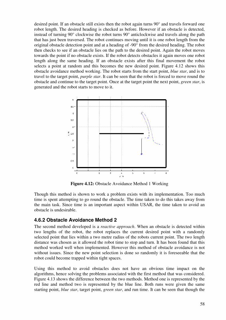
58
desired point. If an obstacle still exists then the robot again turns 90° and travels forward one robot length. The desired heading is checked as before. However if an obstacle is detected, instead of turning 90° clockwise the robot turns 90° anticlockwise and travels along the path that has just been traversed. The robot continues moving until it is one robot length from the original obstacle detection point and at a heading of -90° from the desired heading. The robot then checks to see if an obstacle lies on the path to the desired point. Again the robot moves towards the point if no obstacle exists. If the robot detects obstacles it again moves one robot length along the same heading. If an obstacle exists after this final movement the robot selects a point at random and this becomes the new desired point. Figure 4.12 shows this obstacle avoidance method working. The robot starts from the start point, blue star, and is to travel to the target point, purple star. It can be seen that the robot is forced to move round the obstacle and continue to the target point. Once at the target point the next point, green star, is generated and the robot starts to move to it.
Figure 4.12: Obstacle Avoidance Method 1 Working
Though this method is shown to work a problem exists with its implementation. Too much time is spent attempting to go round the obstacle. The time taken to do this takes away from the main task. Since time is an important aspect within USAR, the time taken to avoid an obstacle is undesirable.
4.6.2 Obstacle Avoidance Method 2
The second method developed is a reactive approach. When an obstacle is detected within two lengths of the robot, the robot replaces the current desired point with a randomly selected point that lies within a two metre radius of the robots current point. The two length distance was chosen as it allowed the robot time to stop and turn. It has been found that this method worked well when implemented. However this method of obstacle avoidance is not without issues. Since the new point selection is done so randomly it is foreseeable that the robot could become trapped within tight spaces. Using this method to avoid obstacles does not have an obvious time impact on the algorithms, hence solving the problems associated with the first method that was considered. Figure 4.13 shows the difference between the two methods. Method one is represented by the red line and method two is represented by the blue line. Both runs were given the same starting point, blue star, target point, green star, and run time. It can be seen that though the
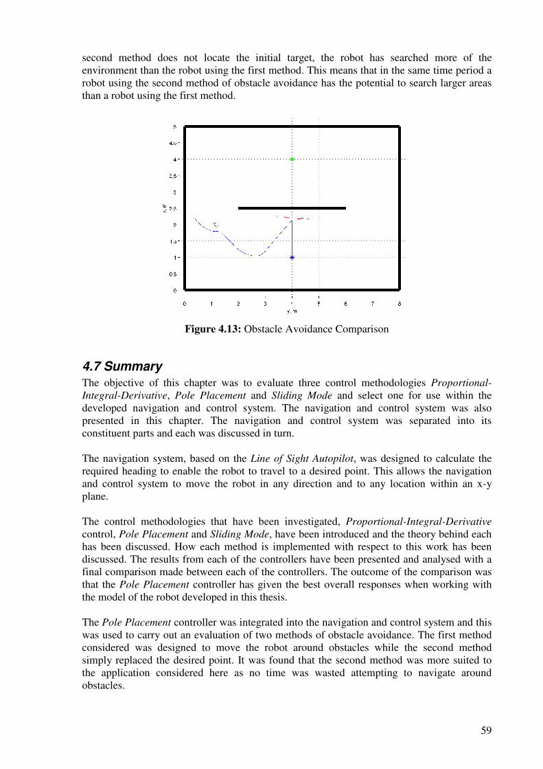
59
second method does not locate the initial target, the robot has searched more of the environment than the robot using the first method. This means that in the same time period a robot using the second method of obstacle avoidance has the potential to search larger areas than a robot using the first method.
Figure 4.13: Obstacle Avoidance Comparison
4.7 Summary
The objective of this chapter was to evaluate three control methodologies Proportional-
Integral-Derivative, Pole Placement and Sliding Mode and select one for use within the developed navigation and control system. The navigation and control system was also presented in this chapter. The navigation and control system was separated into its constituent parts and each was discussed in turn. The navigation system, based on the Line of Sight Autopilot, was designed to calculate the required heading to enable the robot to travel to a desired point. This allows the navigation and control system to move the robot in any direction and to any location within an x-y plane. The control methodologies that have been investigated, Proportional-Integral-Derivative control, Pole Placement and Sliding Mode, have been introduced and the theory behind each has been discussed. How each method is implemented with respect to this work has been discussed. The results from each of the controllers have been presented and analysed with a final comparison made between each of the controllers. The outcome of the comparison was that the Pole Placement controller has given the best overall responses when working with the model of the robot developed in this thesis. The Pole Placement controller was integrated into the navigation and control system and this was used to carry out an evaluation of two methods of obstacle avoidance. The first method considered was designed to move the robot around obstacles while the second method simply replaced the desired point. It was found that the second method was more suited to the application considered here as no time was wasted attempting to navigate around obstacles.
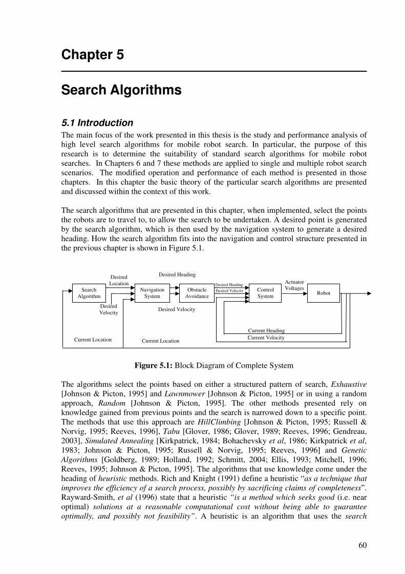
60
Chapter 5
Search Algorithms
5.1 Introduction
The main focus of the work presented in this thesis is the study and performance analysis of high level search algorithms for mobile robot search. In particular, the purpose of this research is to determine the suitability of standard search algorithms for mobile robot searches. In Chapters 6 and 7 these methods are applied to single and multiple robot search scenarios. The modified operation and performance of each method is presented in those chapters. In this chapter the basic theory of the particular search algorithms are presented and discussed within the context of this work. The search algorithms that are presented in this chapter, when implemented, select the points the robots are to travel to, to allow the search to be undertaken. A desired point is generated by the search algorithm, which is then used by the navigation system to generate a desired heading. How the search algorithm fits into the navigation and control structure presented in the previous chapter is shown in Figure 5.1.
Figure 5.1: Block Diagram of Complete System
The algorithms select the points based on either a structured pattern of search, Exhaustive [Johnson & Picton, 1995] and Lawnmower [Johnson & Picton, 1995] or in using a random approach, Random [Johnson & Picton, 1995]. The other methods presented rely on knowledge gained from previous points and the search is narrowed down to a specific point. The methods that use this approach are HillClimbing [Johnson & Picton, 1995; Russell & Norvig, 1995; Reeves, 1996], Tabu [Glover, 1986; Glover, 1989; Reeves, 1996; Gendreau, 2003], Simulated Annealing [Kirkpatrick, 1984; Bohachevsky et al, 1986; Kirkpatrick et al, 1983; Johnson & Picton, 1995; Russell & Norvig, 1995; Reeves, 1996] and Genetic
Algorithms [Goldberg, 1989; Holland, 1992; Schmitt, 2004; Ellis, 1993; Mitchell, 1996; Reeves, 1995; Johnson & Picton, 1995]. The algorithms that use knowledge come under the heading of heuristic methods. Rich and Knight (1991) define a heuristic “as a technique that
improves the efficiency of a search process, possibly by sacrificing claims of completeness”. Rayward-Smith, et al (1996) state that a heuristic “is a method which seeks good (i.e. near optimal) solutions at a reasonable computational cost without being able to guarantee
optimally, and possibly not feasibility”. A heuristic is an algorithm that uses the search
Control System
Current Heading Current Velocity
Desired Velocity
Current Location
Navigation System
Actuator Voltages
Robot Obstacle
Avoidance
Desired Heading
Desired Velocity
Desired Heading
Desired Velocity
Search Algorithm
Desired Location
Current Location
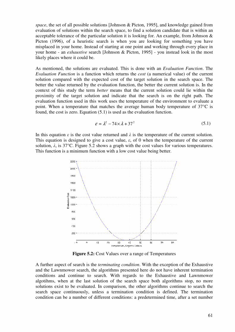
61
space, the set of all possible solutions [Johnson & Picton, 1995], and knowledge gained from evaluation of solutions within the search space, to find a solution candidate that is within an acceptable tolerance of the particular solution it is looking for. An example, from Johnson & Picton (1996), of a heuristic search is when you are looking for something you have misplaced in your home. Instead of starting at one point and working through every place in your home - an exhaustive search [Johnson & Picton, 1995] - you instead look in the most likely places where it could be. As mentioned, the solutions are evaluated. This is done with an Evaluation Function. The Evaluation Function is a function which returns the cost (a numerical value) of the current solution compared with the expected cost of the target solution in the search space. The better the value returned by the evaluation function, the better the current solution is. In the context of this study the term better means that the current solution could lie within the proximity of the target solution and indicate that the search is on the right path. The evaluation function used in this work uses the temperature of the environment to evaluate a point. When a temperature that matches the average human body temperature of 37°C is found, the cost is zero. Equation (5.1) is used as the evaluation function.
22 37+74= λλε ×− (5.1) In this equation ε is the cost value returned and λ is the temperature of the current solution. This equation is designed to give a cost value, ε, of 0 when the temperature of the current solution, λ, is 37°C. Figure 5.2 shows a graph with the cost values for various temperatures. This function is a minimum function with a low cost value being better.
Figure 5.2: Cost Values over a range of Temperatures
A further aspect of search is the terminating condition. With the exception of the Exhaustive and the Lawnmower search, the algorithms presented here do not have inherent termination conditions and continue to search. With regards to the Exhaustive and Lawnmower algotihms, when at the last solution of the search space both algorithms stop, no more solutions exist to be evaluated. In comparison, the other algorithms continue to search the search space continuously, unless a termination condition is defined. The termination condition can be a number of different conditions: a predetermined time, after a set number
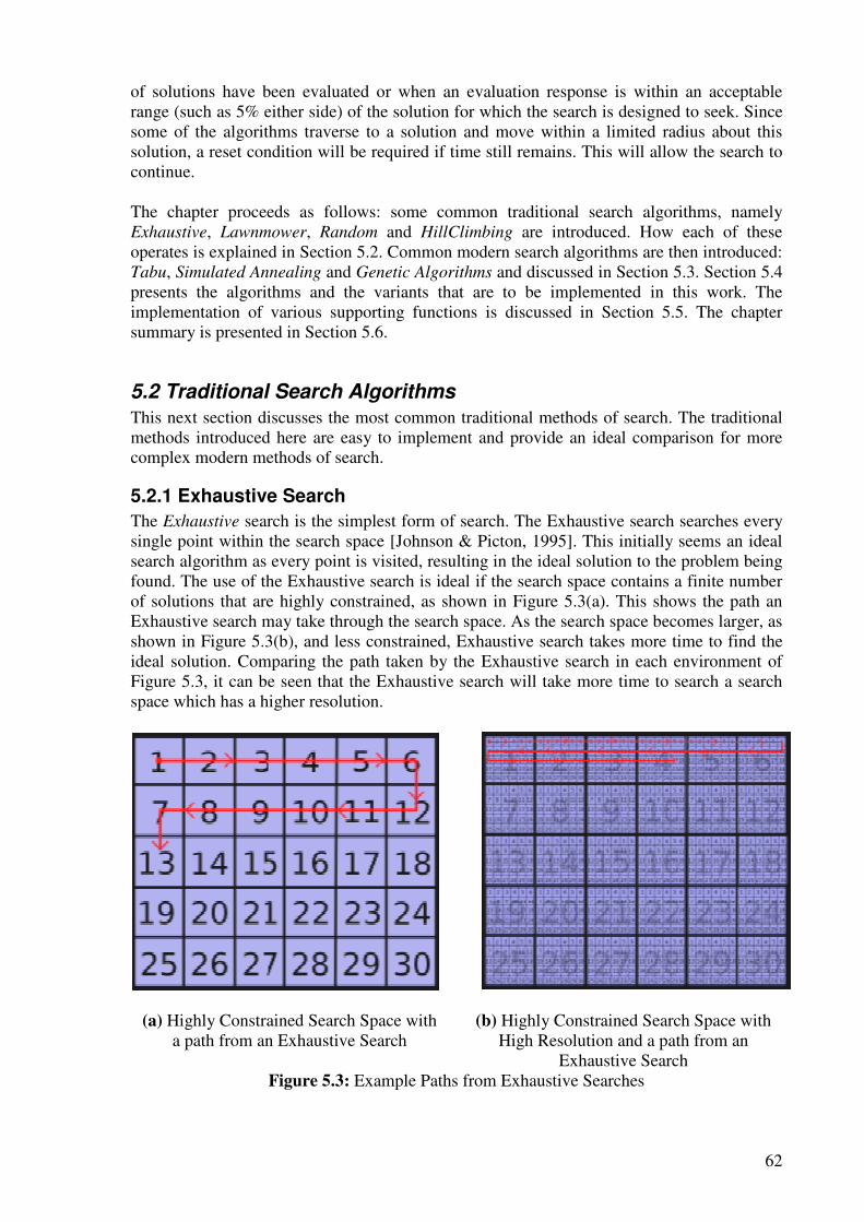
62
of solutions have been evaluated or when an evaluation response is within an acceptable range (such as 5% either side) of the solution for which the search is designed to seek. Since some of the algorithms traverse to a solution and move within a limited radius about this solution, a reset condition will be required if time still remains. This will allow the search to continue. The chapter proceeds as follows: some common traditional search algorithms, namely Exhaustive, Lawnmower, Random and HillClimbing are introduced. How each of these operates is explained in Section 5.2. Common modern search algorithms are then introduced: Tabu, Simulated Annealing and Genetic Algorithms and discussed in Section 5.3. Section 5.4 presents the algorithms and the variants that are to be implemented in this work. The implementation of various supporting functions is discussed in Section 5.5. The chapter summary is presented in Section 5.6.
5.2 Traditional Search Algorithms
This next section discusses the most common traditional methods of search. The traditional methods introduced here are easy to implement and provide an ideal comparison for more complex modern methods of search.
5.2.1 Exhaustive Search
The Exhaustive search is the simplest form of search. The Exhaustive search searches every single point within the search space [Johnson & Picton, 1995]. This initially seems an ideal search algorithm as every point is visited, resulting in the ideal solution to the problem being found. The use of the Exhaustive search is ideal if the search space contains a finite number of solutions that are highly constrained, as shown in Figure 5.3(a). This shows the path an Exhaustive search may take through the search space. As the search space becomes larger, as shown in Figure 5.3(b), and less constrained, Exhaustive search takes more time to find the ideal solution. Comparing the path taken by the Exhaustive search in each environment of Figure 5.3, it can be seen that the Exhaustive search will take more time to search a search space which has a higher resolution.
(a) Highly Constrained Search Space with a path from an Exhaustive Search
(b) Highly Constrained Search Space with High Resolution and a path from an
Exhaustive Search Figure 5.3: Example Paths from Exhaustive Searches
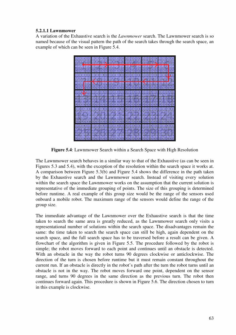
63
5.2.1.1 Lawnmower
A variation of the Exhaustive search is the Lawnmower search. The Lawnmower search is so named because of the visual pattern the path of the search takes through the search space, an example of which can be seen in Figure 5.4.
Figure 5.4: Lawnmower Search within a Search Space with High Resolution The Lawnmower search behaves in a similar way to that of the Exhaustive (as can be seen in Figures 5.3 and 5.4), with the exception of the resolution within the search space it works at. A comparison between Figure 5.3(b) and Figure 5.4 shows the difference in the path taken by the Exhaustive search and the Lawnmower search. Instead of visiting every solution within the search space the Lawnmower works on the assumption that the current solution is representative of the immediate grouping of points. The size of this grouping is determined before runtime. A real example of this group size would be the range of the sensors used onboard a mobile robot. The maximum range of the sensors would define the range of the group size. The immediate advantage of the Lawnmower over the Exhaustive search is that the time taken to search the same area is greatly reduced, as the Lawnmower search only visits a representational number of solutions within the search space. The disadvantages remain the same: the time taken to search the search space can still be high, again dependent on the search space, and the full search space has to be traversed before a result can be given. A flowchart of the algorithm is given in Figure 5.5. The procedure followed by the robot is simple; the robot moves forward to each point and continues until an obstacle is detected. With an obstacle in the way the robot turns 90 degrees clockwise or anticlockwise. The direction of the turn is chosen before runtime but it must remain constant throughout the current run. If an obstacle is directly in the robot’s path after the turn the robot turns until an obstacle is not in the way. The robot moves forward one point, dependent on the sensor range, and turns 90 degrees in the same direction as the previous turn. The robot then continues forward again. This procedure is shown in Figure 5.6. The direction chosen to turn in this example is clockwise.
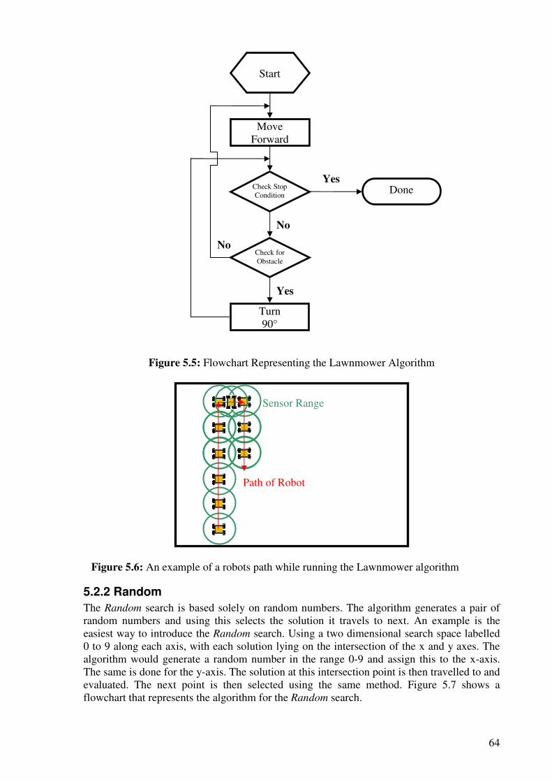
64
Figure 5.5: Flowchart Representing the Lawnmower Algorithm
Figure 5.6: An example of a robots path while running the Lawnmower algorithm
5.2.2 Random
The Random search is based solely on random numbers. The algorithm generates a pair of random numbers and using this selects the solution it travels to next. An example is the easiest way to introduce the Random search. Using a two dimensional search space labelled 0 to 9 along each axis, with each solution lying on the intersection of the x and y axes. The algorithm would generate a random number in the range 0-9 and assign this to the x-axis. The same is done for the y-axis. The solution at this intersection point is then travelled to and evaluated. The next point is then selected using the same method. Figure 5.7 shows a flowchart that represents the algorithm for the Random search.
Sensor Range
Path of Robot
Done
Start
Move Forward
Turn 90°
Check for Obstacle
Check Stop Condition
Yes
Yes
No
No
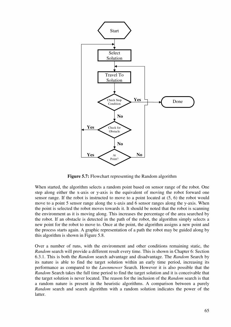
65
Figure 5.7: Flowchart representing the Random algorithm
When started, the algorithm selects a random point based on sensor range of the robot. One step along either the x-axis or y-axis is the equivalent of moving the robot forward one sensor range. If the robot is instructed to move to a point located at (5, 6) the robot would move to a point 5 sensor range along the x-axis and 6 sensor ranges along the y-axis. When the point is selected the robot moves towards it. It should be noted that the robot is scanning the environment as it is moving along. This increases the percentage of the area searched by the robot. If an obstacle is detected in the path of the robot, the algorithm simply selects a new point for the robot to move to. Once at the point, the algorithm assigns a new point and the process starts again. A graphic representation of a path the robot may be guided along by this algorithm is shown in Figure 5.8. Over a number of runs, with the environment and other conditions remaining static, the Random search will provide a different result every time. This is shown in Chapter 6: Section 6.3.1. This is both the Random search advantage and disadvantage. The Random Search by its nature is able to find the target solution within an early time period, increasing its performance as compared to the Lawnmower Search. However it is also possible that the Random Search takes the full time period to find the target solution and it is conceivable that the target solution is never located. The reason for the inclusion of the Random search is that a random nature is present in the heuristic algorithms. A comparison between a purely Random search and search algorithm with a random solution indicates the power of the latter.
At Point?
Done
Start
Select Solution
Travel To Solution
Check for Obstacle
Check Stop Condition
Yes
Yes
No
No
Yes
No
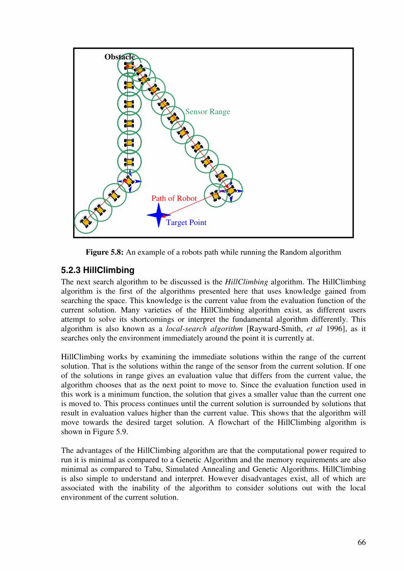
66
Figure 5.8: An example of a robots path while running the Random algorithm
5.2.3 HillClimbing
The next search algorithm to be discussed is the HillClimbing algorithm. The HillClimbing algorithm is the first of the algorithms presented here that uses knowledge gained from searching the space. This knowledge is the current value from the evaluation function of the current solution. Many varieties of the HillClimbing algorithm exist, as different users attempt to solve its shortcomings or interpret the fundamental algorithm differently. This algorithm is also known as a local-search algorithm [Rayward-Smith, et al 1996], as it searches only the environment immediately around the point it is currently at. HillClimbing works by examining the immediate solutions within the range of the current solution. That is the solutions within the range of the sensor from the current solution. If one of the solutions in range gives an evaluation value that differs from the current value, the algorithm chooses that as the next point to move to. Since the evaluation function used in this work is a minimum function, the solution that gives a smaller value than the current one is moved to. This process continues until the current solution is surrounded by solutions that result in evaluation values higher than the current value. This shows that the algorithm will move towards the desired target solution. A flowchart of the HillClimbing algorithm is shown in Figure 5.9. The advantages of the HillClimbing algorithm are that the computational power required to run it is minimal as compared to a Genetic Algorithm and the memory requirements are also minimal as compared to Tabu, Simulated Annealing and Genetic Algorithms. HillClimbing is also simple to understand and interpret. However disadvantages exist, all of which are associated with the inability of the algorithm to consider solutions out with the local environment of the current solution.
Sensor Range
Path of Robot
Target Point
Obstacle
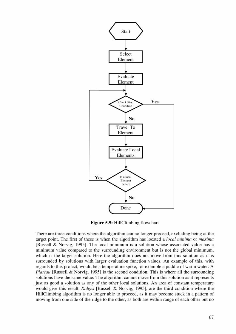
67
Figure 5.9: HillClimbing flowchart There are three conditions where the algorithm can no longer proceed, excluding being at the target point. The first of these is when the algorithm has located a local minima or maxima [Russell & Norvig, 1995]. The local minimum is a solution whose associated value has a minimum value compared to the surrounding environment but is not the global minimum, which is the target solution. Here the algorithm does not move from this solution as it is surrounded by solutions with larger evaluation function values. An example of this, with regards to this project, would be a temperature spike, for example a puddle of warm water. A Plateau [Russell & Norvig, 1995] is the second condition. This is where all the surrounding solutions have the same value. The algorithm cannot move from this solution as it represents just as good a solution as any of the other local solutions. An area of constant temperature would give this result. Ridges [Russell & Norvig, 1995], are the third condition where the HillClimbing algorithm is no longer able to proceed, as it may become stuck in a pattern of moving from one side of the ridge to the other, as both are within range of each other but no
Is a local Element better?
Done
Start
Select Element
Travel To Element
Check Stop Condition
Yes
No
No
Yes
Evaluate Element
Evaluate Local Elements
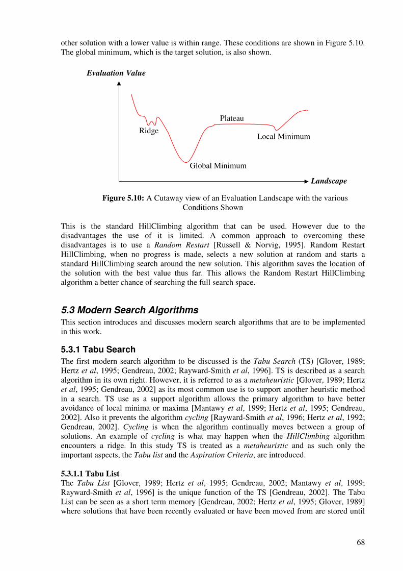
68
other solution with a lower value is within range. These conditions are shown in Figure 5.10. The global minimum, which is the target solution, is also shown.
Figure 5.10: A Cutaway view of an Evaluation Landscape with the various Conditions Shown
This is the standard HillClimbing algorithm that can be used. However due to the disadvantages the use of it is limited. A common approach to overcoming these disadvantages is to use a Random Restart [Russell & Norvig, 1995]. Random Restart HillClimbing, when no progress is made, selects a new solution at random and starts a standard HillClimbing search around the new solution. This algorithm saves the location of the solution with the best value thus far. This allows the Random Restart HillClimbing
algorithm a better chance of searching the full search space.
5.3 Modern Search Algorithms
This section introduces and discusses modern search algorithms that are to be implemented in this work.
5.3.1 Tabu Search
The first modern search algorithm to be discussed is the Tabu Search (TS) [Glover, 1989; Hertz et al, 1995; Gendreau, 2002; Rayward-Smith et al, 1996]. TS is described as a search algorithm in its own right. However, it is referred to as a metaheuristic [Glover, 1989; Hertz et al, 1995; Gendreau, 2002] as its most common use is to support another heuristic method in a search. TS use as a support algorithm allows the primary algorithm to have better avoidance of local minima or maxima [Mantawy et al, 1999; Hertz et al, 1995; Gendreau, 2002]. Also it prevents the algorithm cycling [Rayward-Smith et al, 1996; Hertz et al, 1992; Gendreau, 2002]. Cycling is when the algorithm continually moves between a group of solutions. An example of cycling is what may happen when the HillClimbing algorithm encounters a ridge. In this study TS is treated as a metaheuristic and as such only the important aspects, the Tabu list and the Aspiration Criteria, are introduced. 5.3.1.1 Tabu List
The Tabu List [Glover, 1989; Hertz et al, 1995; Gendreau, 2002; Mantawy et al, 1999; Rayward-Smith et al, 1996] is the unique function of the TS [Gendreau, 2002]. The Tabu List can be seen as a short term memory [Gendreau, 2002; Hertz et al, 1995; Glover, 1989] where solutions that have been recently evaluated or have been moved from are stored until
Global Minimum
Plateau
Ridge Local Minimum
Evaluation Value
Landscape
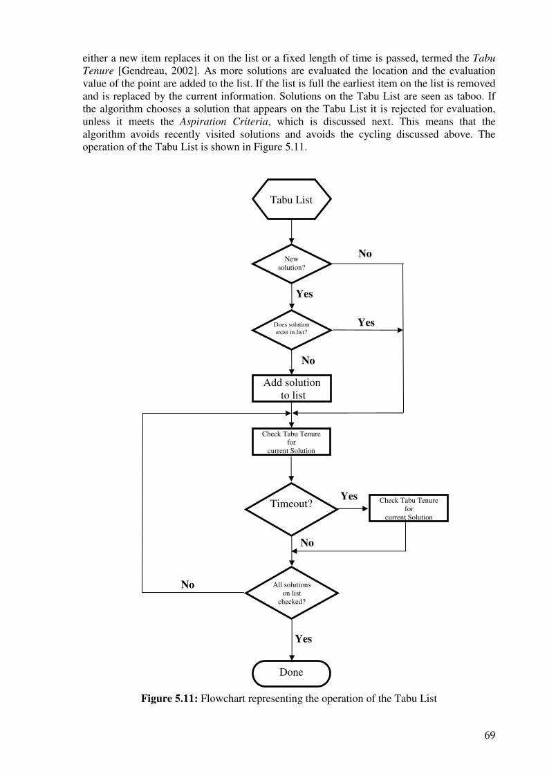
69
either a new item replaces it on the list or a fixed length of time is passed, termed the Tabu
Tenure [Gendreau, 2002]. As more solutions are evaluated the location and the evaluation value of the point are added to the list. If the list is full the earliest item on the list is removed and is replaced by the current information. Solutions on the Tabu List are seen as taboo. If the algorithm chooses a solution that appears on the Tabu List it is rejected for evaluation, unless it meets the Aspiration Criteria, which is discussed next. This means that the algorithm avoids recently visited solutions and avoids the cycling discussed above. The operation of the Tabu List is shown in Figure 5.11.
Figure 5.11: Flowchart representing the operation of the Tabu List
Timeout?
Done
Tabu List
Add solution to list
Does solution exist in list?
Yes
No
No
Yes
Check Tabu Tenure for
current Solution
New solution?
No
Yes
All solutions on list
checked?
Check Tabu Tenure for
current Solution
No
Yes
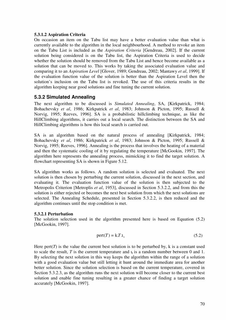
70
5.3.1.2 Aspiration Criteria
On occasion an item on the Tabu list may have a better evaluation value than what is currently available to the algorithm in the local neighbourhood. A method to revoke an item on the Tabu List is included as the Aspiration Criteria [Gendreau, 2002]. If the current solution being considered is on the Tabu list, the Aspiration Criteria is used to decide whether the solution should be removed from the Tabu List and hence become available as a solution that can be moved to. This works by taking the associated evaluation value and comparing it to an Aspiration Level [Glover, 1989; Gendreau, 2002; Mantawy et al, 1999]. If the evaluation function value of the solution is better than the Aspiration Level then the solution’s inclusion on the Tabu list is revoked. The use of this criteria results in the algorithm keeping near good solutions and fine tuning the current solution.
5.3.2 Simulated Annealing
The next algorithm to be discussed is Simulated Annealing, SA, [Kirkpatrick, 1984; Bohachevsky et al, 1986; Kirkpatrick et al, 1983; Johnson & Picton, 1995; Russell & Norvig, 1995; Reeves, 1996]. SA is a probabilistic hillclimbing technique, as like the HillClimbing algorithms, it carries out a local search. The distinction between the SA and HillClimbing algorithms is how this local search is carried out. SA is an algorithm based on the natural process of annealing [Kirkpatrick, 1984; Bohachevsky et al, 1986; Kirkpatrick et al, 1983; Johnson & Picton, 1995; Russell & Norvig, 1995; Reeves, 1996]. Annealing is the process that involves the heating of a material and then the systematic cooling of it by regulating the temperature [McGookin, 1997]. The algorithm here represents the annealing process, mimicking it to find the target solution. A flowchart representing SA is shown in Figure 5.12. SA algorithm works as follows. A random solution is selected and evaluated. The next solution is then chosen by perturbing the current solution, discussed in the next section, and evaluating it. The evaluation function value of the solution is then subjected to the Metropolis Criterion [Metroplis et al, 1953], discussed in Section 5.3.2.2, and from this the solution is either rejected or becomes the next best solution from which the next solutions are selected. The Annealing Schedule, presented in Section 5.3.2.2, is then reduced and the algorithm continues until the stop condition is met. 5.3.2.1 Perturbation
The solution selection used in the algorithm presented here is based on Equation (5.2) [McGookin, 1997].
r..k=)(pert ιTT (5.2)
Here pert(T) is the value the current best solution is to be perturbed by, k is a constant used to scale the result, T is the current temperature and ιr is a random number between 0 and 1. By selecting the next solution in this way keeps the algorithm within the range of a solution with a good evaluation value but still letting it hunt around the immediate area for another better solution. Since the solution selection is based on the current temperature, covered in Section 5.3.2.3, as the algorithm runs the next solution will become closer to the current best solution and enable fine tuning resulting in a greater chance of finding a target solution accurately [McGookin, 1997].
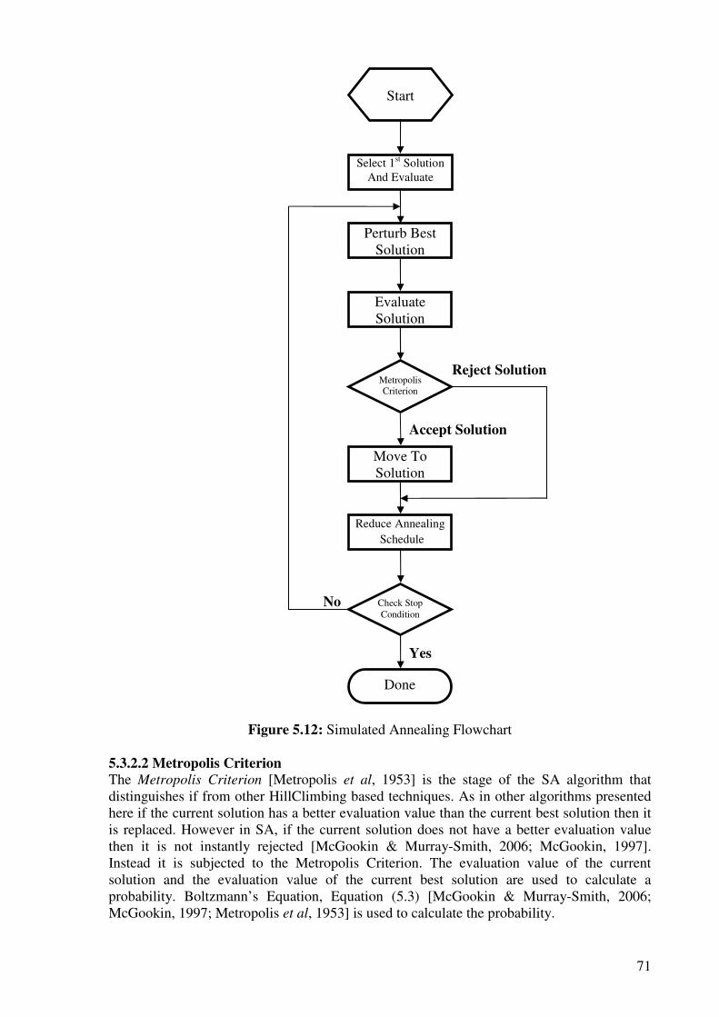
71
Figure 5.12: Simulated Annealing Flowchart 5.3.2.2 Metropolis Criterion
The Metropolis Criterion [Metropolis et al, 1953] is the stage of the SA algorithm that distinguishes if from other HillClimbing based techniques. As in other algorithms presented here if the current solution has a better evaluation value than the current best solution then it is replaced. However in SA, if the current solution does not have a better evaluation value then it is not instantly rejected [McGookin & Murray-Smith, 2006; McGookin, 1997]. Instead it is subjected to the Metropolis Criterion. The evaluation value of the current solution and the evaluation value of the current best solution are used to calculate a probability. Boltzmann’s Equation, Equation (5.3) [McGookin & Murray-Smith, 2006; McGookin, 1997; Metropolis et al, 1953] is used to calculate the probability.
Start
Select 1st Solution And Evaluate
Reduce Annealing
Schedule
Metropolis Criterion
Accept Solution
Perturb Best Solution
Move To Solution
Evaluate Solution
Reject Solution
Yes
No Check Stop Condition
Done
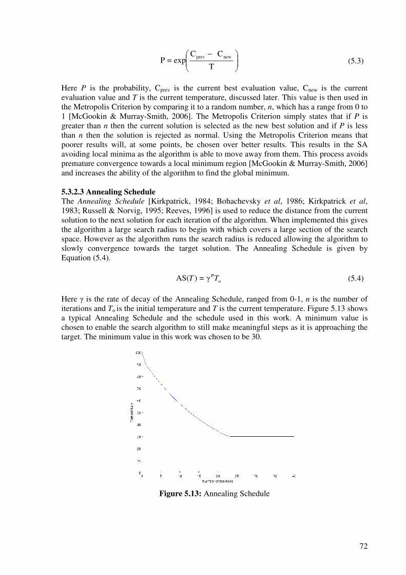
72
−
T
CCexp=P newprev (5.3)
Here P is the probability, Cprev is the current best evaluation value, Cnew is the current evaluation value and T is the current temperature, discussed later. This value is then used in the Metropolis Criterion by comparing it to a random number, n, which has a range from 0 to 1 [McGookin & Murray-Smith, 2006]. The Metropolis Criterion simply states that if P is greater than n then the current solution is selected as the new best solution and if P is less than n then the solution is rejected as normal. Using the Metropolis Criterion means that poorer results will, at some points, be chosen over better results. This results in the SA avoiding local minima as the algorithm is able to move away from them. This process avoids premature convergence towards a local minimum region [McGookin & Murray-Smith, 2006] and increases the ability of the algorithm to find the global minimum. 5.3.2.3 Annealing Schedule
The Annealing Schedule [Kirkpatrick, 1984; Bohachevsky et al, 1986; Kirkpatrick et al, 1983; Russell & Norvig, 1995; Reeves, 1996] is used to reduce the distance from the current solution to the next solution for each iteration of the algorithm. When implemented this gives the algorithm a large search radius to begin with which covers a large section of the search space. However as the algorithm runs the search radius is reduced allowing the algorithm to slowly convergence towards the target solution. The Annealing Schedule is given by Equation (5.4).
oγ=)AS( TTn (5.4)
Here γ is the rate of decay of the Annealing Schedule, ranged from 0-1, n is the number of iterations and To is the initial temperature and T is the current temperature. Figure 5.13 shows a typical Annealing Schedule and the schedule used in this work. A minimum value is chosen to enable the search algorithm to still make meaningful steps as it is approaching the target. The minimum value in this work was chosen to be 30.
Figure 5.13: Annealing Schedule
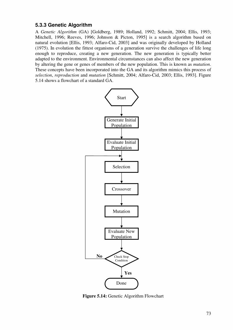
73
5.3.3 Genetic Algorithm
A Genetic Algorithm (GA) [Goldberg, 1989; Holland, 1992; Schmitt, 2004; Ellis, 1993; Mitchell, 1996; Reeves, 1996; Johnson & Picton, 1995] is a search algorithm based on natural evolution [Ellis, 1993; Alfaro-Cid, 2003] and was originally developed by Holland (1975). In evolution the fittest organisms of a generation survive the challenges of life long enough to reproduce, creating a new generation. The new generation is typically better adapted to the environment. Environmental circumstances can also affect the new generation by altering the gene or genes of members of the new population. This is known as mutation. These concepts have been incorporated into the GA and its algorithm mimics this process of selection, reproduction and mutation [Schmitt, 2004; Alfaro-Cid, 2003; Ellis, 1993]. Figure 5.14 shows a flowchart of a standard GA.
Figure 5.14: Genetic Algorithm Flowchart
Done
Start
Generate Initial Population
Yes
No
Selection
Crossover
Check Stop Condition
Evaluate Initial Population
Mutation
Evaluate New Population
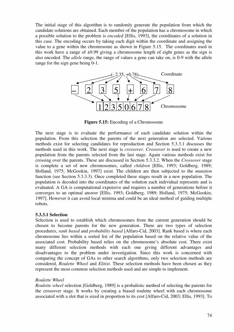
74
The initial stage of this algorithm is to randomly generate the population from which the candidate solutions are obtained. Each member of the population has a chromosome in which a possible solution to the problem is encoded [Ellis, 1993], the coordinates of a solution in this case. The encoding occurs by taking each digit within the coordinate and assigning the value to a gene within the chromosome as shown in Figure 5.15. The coordinates used in this work have a range of ±9.99 giving a chromosome length of eight genes as the sign is also encoded. The allele range, the range of values a gene can take on, is 0-9 with the allele range for the sign gene being 0-1.
Figure 5.15: Encoding of a Chromosome The next stage is to evaluate the performance of each candidate solution within the population. From this selection the parents of the next generation are selected. Various methods exist for selecting candidates for reproduction and Section 5.3.3.1 discusses the methods used in this work. The next stage is crossover. Crossover is used to create a new population from the parents selected from the last stage. Again various methods exist for crossing over the parents. These are discussed in Section 5.3.3.2. When the Crossover stage is complete a set of new chromosomes, called children [Ellis, 1993; Goldberg, 1989; Holland, 1975; McGookin, 1997] exist. The children are then subjected to the mutation function (see Section 5.3.3.3). Once completed these stages result in a new population. The population is decoded into the coordinates of the solution each individual represents and is evaluated. A GA is computational expensive and requires a number of generations before it converges to an optimal answer [Ellis, 1993; Goldberg, 1989; Holland, 1975; McGookin, 1997]. However it can avoid local minima and could be an ideal method of guiding multiple robots. 5.3.3.1 Selection
Selection is used to establish which chromosomes from the current generation should be chosen to become parents for the new generation. There are two types of selection procedures, rank based and probability based [Alfaro-Cid, 2003]. Rank based is where each chromosome lies within a sorted list of the population based on the relative value of the associated cost. Probability based relies on the chromosome’s absolute cost. There exist many different selection methods with each one giving different advantages and disadvantages to the problem under investigation. Since this work is concerned with comparing the concept of GAs to other search algorithms, only two selection methods are considered, Roulette Wheel and Elitist. These selection methods have been chosen as they represent the most common selection methods used and are simple to implement. Roulette Wheel
Roulette wheel selection [Goldberg, 1989] is a probalistic method of selecting the parents for the crossover stage. It works by creating a biased roulette wheel with each chromosome associated with a slot that is sized in proportion to its cost [Alfaro-Cid, 2003; Ellis, 1993]. To
1 2 3 5 0 6 7 8 Chromosome
(- 2.35, +6.78) Coordinate
− 2 3 5 + 6 7 8
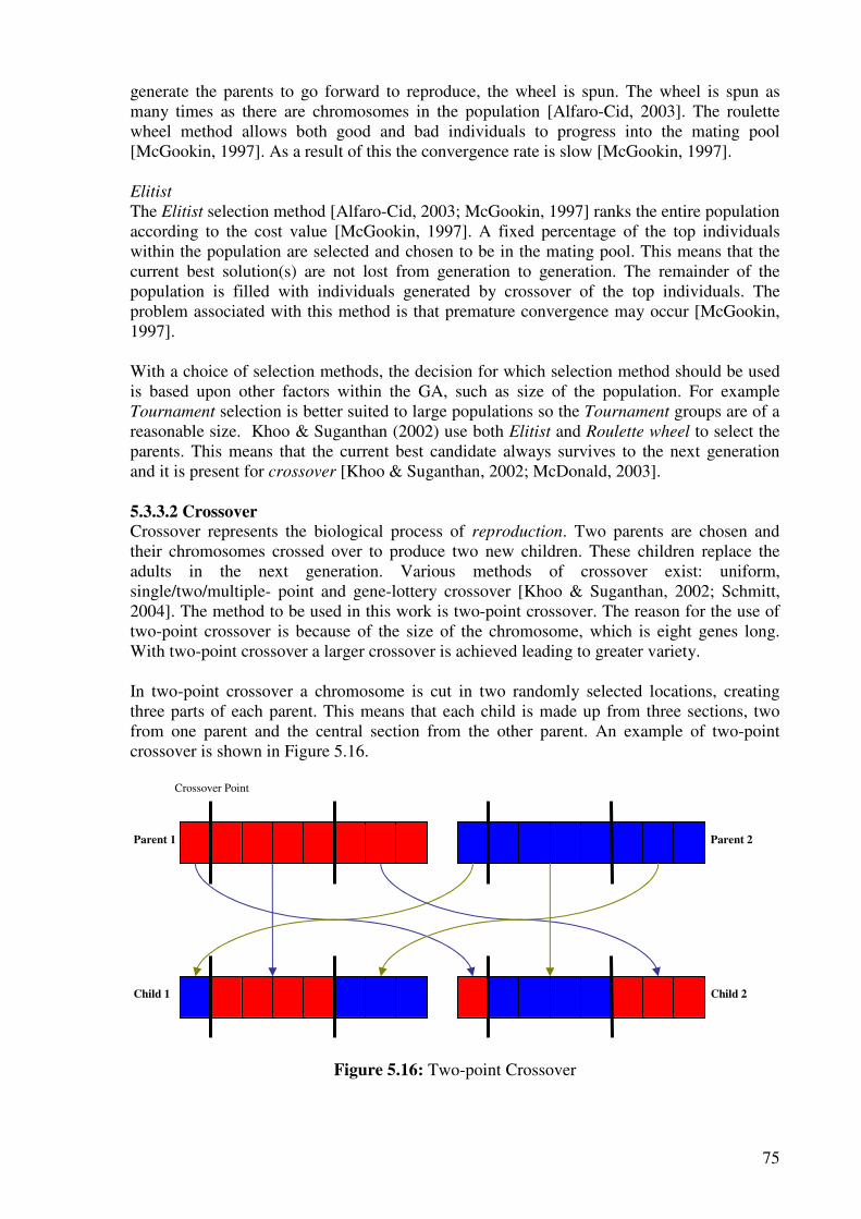
75
generate the parents to go forward to reproduce, the wheel is spun. The wheel is spun as many times as there are chromosomes in the population [Alfaro-Cid, 2003]. The roulette wheel method allows both good and bad individuals to progress into the mating pool [McGookin, 1997]. As a result of this the convergence rate is slow [McGookin, 1997]. Elitist
The Elitist selection method [Alfaro-Cid, 2003; McGookin, 1997] ranks the entire population according to the cost value [McGookin, 1997]. A fixed percentage of the top individuals within the population are selected and chosen to be in the mating pool. This means that the current best solution(s) are not lost from generation to generation. The remainder of the population is filled with individuals generated by crossover of the top individuals. The problem associated with this method is that premature convergence may occur [McGookin, 1997]. With a choice of selection methods, the decision for which selection method should be used is based upon other factors within the GA, such as size of the population. For example Tournament selection is better suited to large populations so the Tournament groups are of a reasonable size. Khoo & Suganthan (2002) use both Elitist and Roulette wheel to select the parents. This means that the current best candidate always survives to the next generation and it is present for crossover [Khoo & Suganthan, 2002; McDonald, 2003]. 5.3.3.2 Crossover
Crossover represents the biological process of reproduction. Two parents are chosen and their chromosomes crossed over to produce two new children. These children replace the adults in the next generation. Various methods of crossover exist: uniform, single/two/multiple- point and gene-lottery crossover [Khoo & Suganthan, 2002; Schmitt, 2004]. The method to be used in this work is two-point crossover. The reason for the use of two-point crossover is because of the size of the chromosome, which is eight genes long. With two-point crossover a larger crossover is achieved leading to greater variety. In two-point crossover a chromosome is cut in two randomly selected locations, creating three parts of each parent. This means that each child is made up from three sections, two from one parent and the central section from the other parent. An example of two-point crossover is shown in Figure 5.16.
Figure 5.16: Two-point Crossover
Crossover Point
Parent 1
Child 1 Child 2
Parent 2
76
McDonald (2003) suggests that single point crossover is perceived to be the most appropriate crossover method due to the popularity of it and says that crossover schemes that use more than one point increase the chance of a fit individual being disrupted [McDonald, 2003]. This increases the convergence time, a stance supported by Dejong’s (1975) work that concludes that a GA’s overall performance degrades as the number of crossover points increases. Alfaro-Cid (2003) suggests that with conservative selection methods, as used by Dejong (1975), increased crossover points do degrade a GA’s performance. With strong selection schemes using two-point or multiple-point crossover is shown to work [Alfaro-Cid, 2003]. This again shows that the operators and structure of the GAs can vary the performance. A study of how uniform, single point and multi point crossover compare can be found in Khoo and Suganthan (2002). 5.3.3.3 Mutation
Mutation slightly alters a child or children generated by the crossover [Ellis, 1993; Alfaro-Cid, 2003; Holland, 1975; McGookin, 1997]. The most basic mutation operator chooses one or more genes in a member of the population and the allele, the value of that gene, is replaced with a randomly generated value [Alfaro-Cid, 2003]. A mutation happens with reference to a mutation rate [Ellis, 1993; Alfaro-Cid, 2003; Holland, 1975; McGookin, 1997]. The mutation rate is a value representing the percentage of the population that is to be mutated during a single iteration of the GA. There are various schools of thought on what value should be given to the mutation rate. A high mutation rate could keep the algorithm away from a target point by continually jumping away from it, but a low mutation rate may not find the target as values that have been removed may not be reintroduced [Ellis, 1993]. The mutation rate, in simple GAs, is normally kept the same until the termination of the algorithm. Other GA schemes have experimented with time varying mutation rates. Khoo & Sugantham (2002) present a method where the mutation rate is reduced near the end of the simulation run. The presented argument is that a high mutation rate at the beginning leads to a diverse population and a low mutation rate at the end means that good solutions are not destroyed [Khoo and Suganthan, 2002]. A large number of different GAs can be created, however the work here will only look at four combinations. The combinations selected will be based on the selection methods discussed: Roulette Wheel and Elitist, two-point crossover and two values for the mutation rate, low (0.1%) and high (10%).
5.4 Algorithms and Variants to be Implemented
The theory of each algorithm selected for this work has been discussed. The next stage is to define the variations of the algorithms that are to be used. This is included to clarify the algorithms that are studied. Though it is not implicitly stated, each algorithm scans for solutions of interest within a set range of the mobile robot while travelling to each solution selected by the algorithm. This allows a more extensive search to be carried out. If a solution of interest is noted along the path then a judgement is made whether or not the robot should travel to it. The judgement is made based on the temperature being detected at the point from a distance.
5.4.1 Lawnmower
The standard Lawnmower algorithm is used with no variations or adaptation.
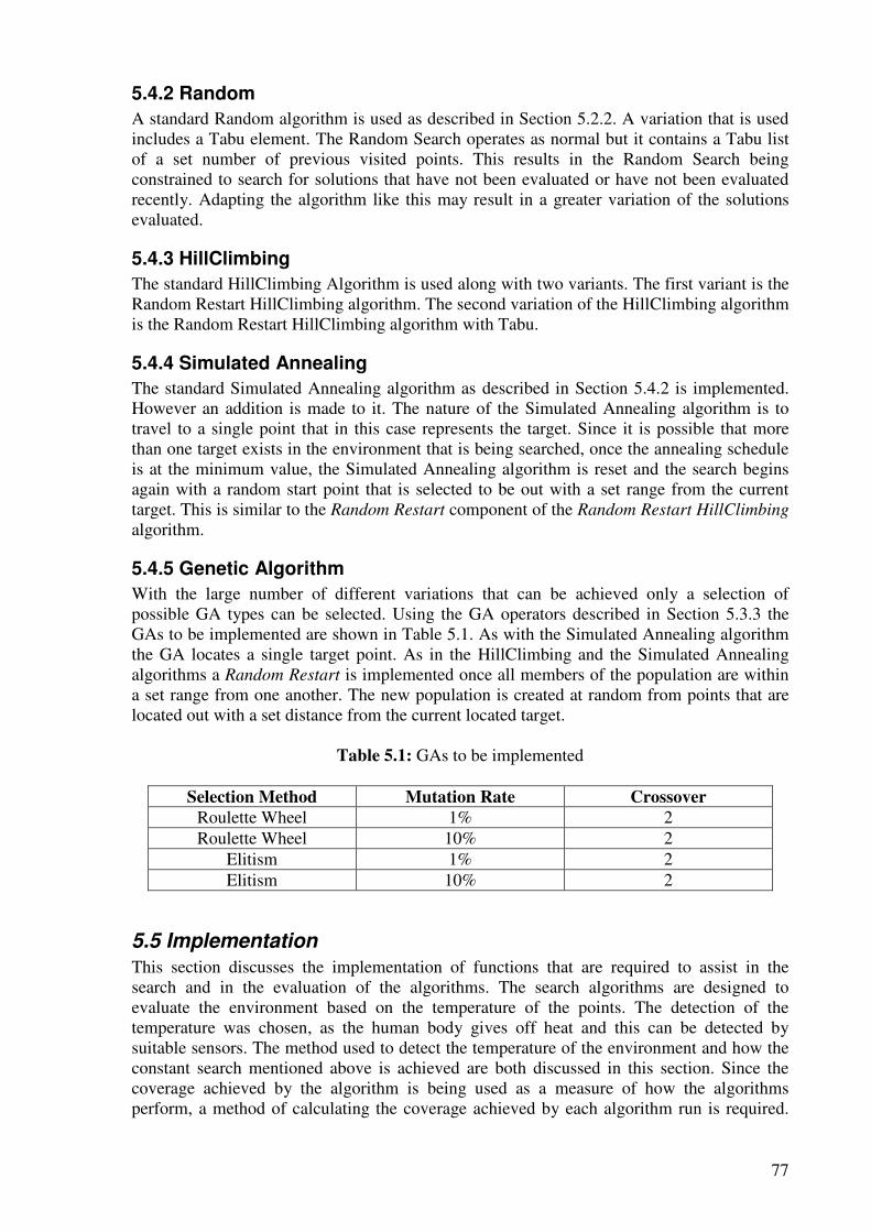
77
5.4.2 Random
A standard Random algorithm is used as described in Section 5.2.2. A variation that is used includes a Tabu element. The Random Search operates as normal but it contains a Tabu list of a set number of previous visited points. This results in the Random Search being constrained to search for solutions that have not been evaluated or have not been evaluated recently. Adapting the algorithm like this may result in a greater variation of the solutions evaluated.
5.4.3 HillClimbing
The standard HillClimbing Algorithm is used along with two variants. The first variant is the Random Restart HillClimbing algorithm. The second variation of the HillClimbing algorithm is the Random Restart HillClimbing algorithm with Tabu.
5.4.4 Simulated Annealing
The standard Simulated Annealing algorithm as described in Section 5.4.2 is implemented. However an addition is made to it. The nature of the Simulated Annealing algorithm is to travel to a single point that in this case represents the target. Since it is possible that more than one target exists in the environment that is being searched, once the annealing schedule is at the minimum value, the Simulated Annealing algorithm is reset and the search begins again with a random start point that is selected to be out with a set range from the current target. This is similar to the Random Restart component of the Random Restart HillClimbing
algorithm.
5.4.5 Genetic Algorithm
With the large number of different variations that can be achieved only a selection of possible GA types can be selected. Using the GA operators described in Section 5.3.3 the GAs to be implemented are shown in Table 5.1. As with the Simulated Annealing algorithm the GA locates a single target point. As in the HillClimbing and the Simulated Annealing algorithms a Random Restart is implemented once all members of the population are within a set range from one another. The new population is created at random from points that are located out with a set distance from the current located target.
Table 5.1: GAs to be implemented
Selection Method Mutation Rate Crossover
Roulette Wheel 1% 2 Roulette Wheel 10% 2
Elitism 1% 2 Elitism 10% 2
5.5 Implementation
This section discusses the implementation of functions that are required to assist in the search and in the evaluation of the algorithms. The search algorithms are designed to evaluate the environment based on the temperature of the points. The detection of the temperature was chosen, as the human body gives off heat and this can be detected by suitable sensors. The method used to detect the temperature of the environment and how the constant search mentioned above is achieved are both discussed in this section. Since the coverage achieved by the algorithm is being used as a measure of how the algorithms perform, a method of calculating the coverage achieved by each algorithm run is required.
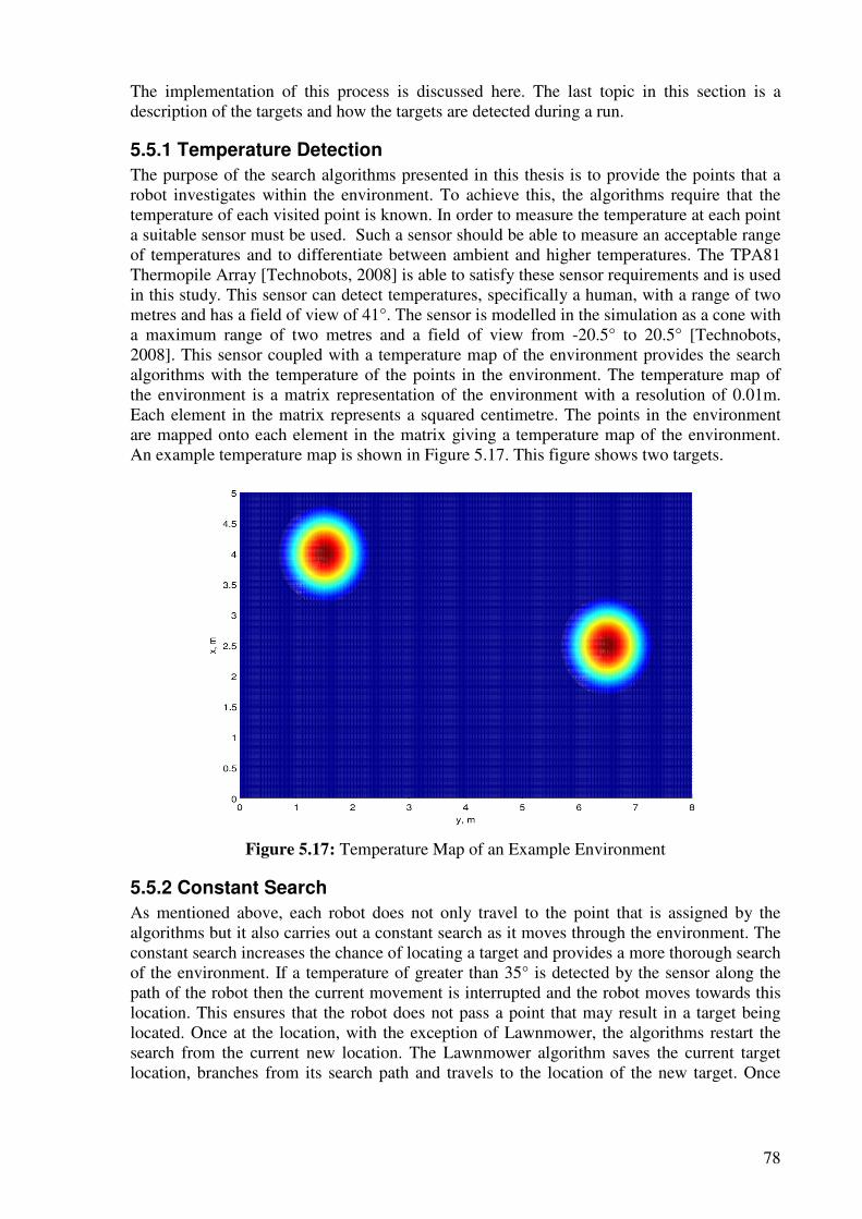
78
The implementation of this process is discussed here. The last topic in this section is a description of the targets and how the targets are detected during a run.
5.5.1 Temperature Detection
The purpose of the search algorithms presented in this thesis is to provide the points that a robot investigates within the environment. To achieve this, the algorithms require that the temperature of each visited point is known. In order to measure the temperature at each point a suitable sensor must be used. Such a sensor should be able to measure an acceptable range of temperatures and to differentiate between ambient and higher temperatures. The TPA81 Thermopile Array [Technobots, 2008] is able to satisfy these sensor requirements and is used in this study. This sensor can detect temperatures, specifically a human, with a range of two metres and has a field of view of 41°. The sensor is modelled in the simulation as a cone with a maximum range of two metres and a field of view from -20.5° to 20.5° [Technobots, 2008]. This sensor coupled with a temperature map of the environment provides the search algorithms with the temperature of the points in the environment. The temperature map of the environment is a matrix representation of the environment with a resolution of 0.01m. Each element in the matrix represents a squared centimetre. The points in the environment are mapped onto each element in the matrix giving a temperature map of the environment. An example temperature map is shown in Figure 5.17. This figure shows two targets.
Figure 5.17: Temperature Map of an Example Environment
5.5.2 Constant Search
As mentioned above, each robot does not only travel to the point that is assigned by the algorithms but it also carries out a constant search as it moves through the environment. The constant search increases the chance of locating a target and provides a more thorough search of the environment. If a temperature of greater than 35° is detected by the sensor along the path of the robot then the current movement is interrupted and the robot moves towards this location. This ensures that the robot does not pass a point that may result in a target being located. Once at the location, with the exception of Lawnmower, the algorithms restart the search from the current new location. The Lawnmower algorithm saves the current target location, branches from its search path and travels to the location of the new target. Once
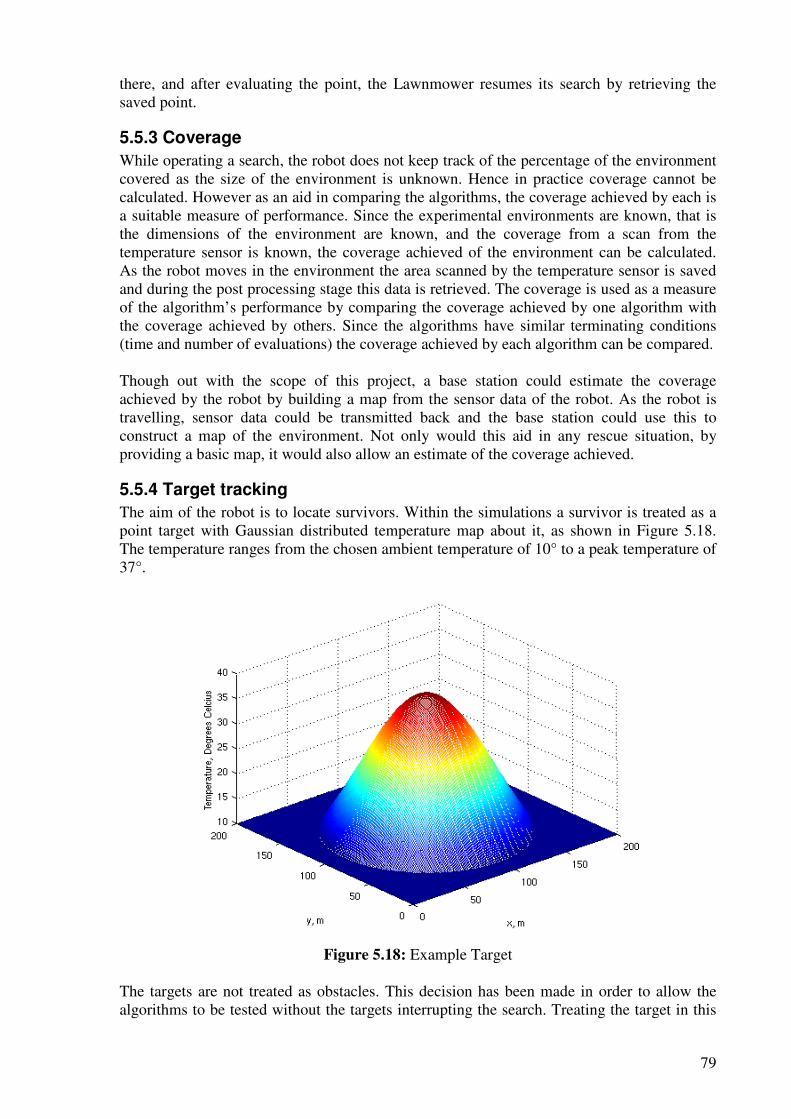
79
there, and after evaluating the point, the Lawnmower resumes its search by retrieving the saved point.
5.5.3 Coverage
While operating a search, the robot does not keep track of the percentage of the environment covered as the size of the environment is unknown. Hence in practice coverage cannot be calculated. However as an aid in comparing the algorithms, the coverage achieved by each is a suitable measure of performance. Since the experimental environments are known, that is the dimensions of the environment are known, and the coverage from a scan from the temperature sensor is known, the coverage achieved of the environment can be calculated. As the robot moves in the environment the area scanned by the temperature sensor is saved and during the post processing stage this data is retrieved. The coverage is used as a measure of the algorithm’s performance by comparing the coverage achieved by one algorithm with the coverage achieved by others. Since the algorithms have similar terminating conditions (time and number of evaluations) the coverage achieved by each algorithm can be compared. Though out with the scope of this project, a base station could estimate the coverage achieved by the robot by building a map from the sensor data of the robot. As the robot is travelling, sensor data could be transmitted back and the base station could use this to construct a map of the environment. Not only would this aid in any rescue situation, by providing a basic map, it would also allow an estimate of the coverage achieved.
5.5.4 Target tracking
The aim of the robot is to locate survivors. Within the simulations a survivor is treated as a point target with Gaussian distributed temperature map about it, as shown in Figure 5.18. The temperature ranges from the chosen ambient temperature of 10° to a peak temperature of 37°.
Figure 5.18: Example Target
The targets are not treated as obstacles. This decision has been made in order to allow the algorithms to be tested without the targets interrupting the search. Treating the target in this
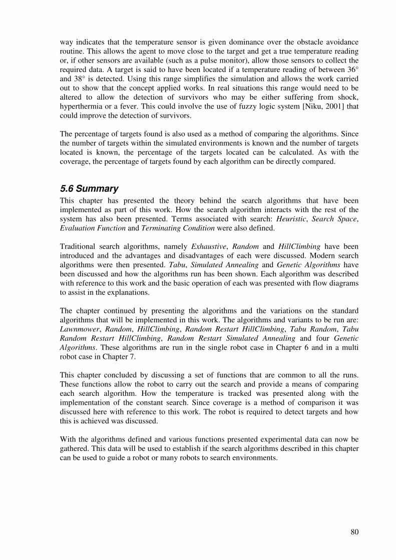
80
way indicates that the temperature sensor is given dominance over the obstacle avoidance routine. This allows the agent to move close to the target and get a true temperature reading or, if other sensors are available (such as a pulse monitor), allow those sensors to collect the required data. A target is said to have been located if a temperature reading of between 36° and 38° is detected. Using this range simplifies the simulation and allows the work carried out to show that the concept applied works. In real situations this range would need to be altered to allow the detection of survivors who may be either suffering from shock, hyperthermia or a fever. This could involve the use of fuzzy logic system [Niku, 2001] that could improve the detection of survivors. The percentage of targets found is also used as a method of comparing the algorithms. Since the number of targets within the simulated environments is known and the number of targets located is known, the percentage of the targets located can be calculated. As with the coverage, the percentage of targets found by each algorithm can be directly compared.
5.6 Summary
This chapter has presented the theory behind the search algorithms that have been implemented as part of this work. How the search algorithm interacts with the rest of the system has also been presented. Terms associated with search: Heuristic, Search Space, Evaluation Function and Terminating Condition were also defined. Traditional search algorithms, namely Exhaustive, Random and HillClimbing have been introduced and the advantages and disadvantages of each were discussed. Modern search algorithms were then presented. Tabu, Simulated Annealing and Genetic Algorithms have been discussed and how the algorithms run has been shown. Each algorithm was described with reference to this work and the basic operation of each was presented with flow diagrams to assist in the explanations. The chapter continued by presenting the algorithms and the variations on the standard algorithms that will be implemented in this work. The algorithms and variants to be run are: Lawnmower, Random, HillClimbing, Random Restart HillClimbing, Tabu Random, Tabu
Random Restart HillClimbing, Random Restart Simulated Annealing and four Genetic
Algorithms. These algorithms are run in the single robot case in Chapter 6 and in a multi robot case in Chapter 7. This chapter concluded by discussing a set of functions that are common to all the runs. These functions allow the robot to carry out the search and provide a means of comparing each search algorithm. How the temperature is tracked was presented along with the implementation of the constant search. Since coverage is a method of comparison it was discussed here with reference to this work. The robot is required to detect targets and how this is achieved was discussed. With the algorithms defined and various functions presented experimental data can now be gathered. This data will be used to establish if the search algorithms described in this chapter can be used to guide a robot or many robots to search environments.
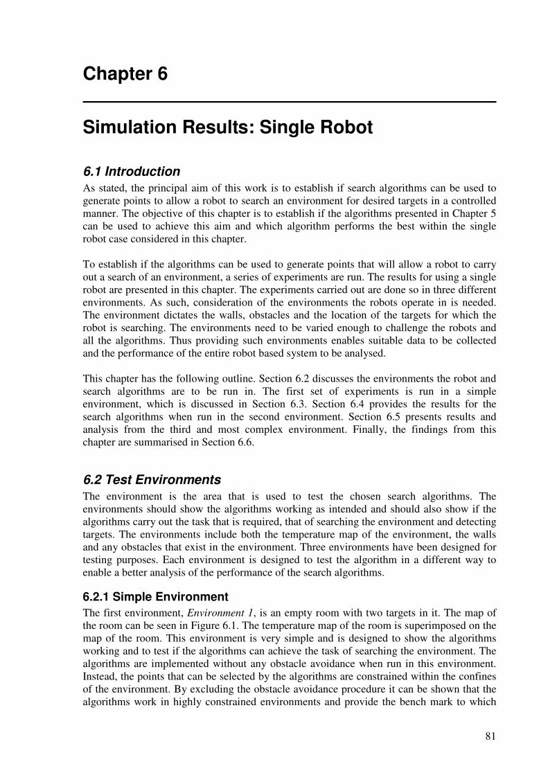
81
Chapter 6
Simulation Results: Single Robot
6.1 Introduction
As stated, the principal aim of this work is to establish if search algorithms can be used to generate points to allow a robot to search an environment for desired targets in a controlled manner. The objective of this chapter is to establish if the algorithms presented in Chapter 5 can be used to achieve this aim and which algorithm performs the best within the single robot case considered in this chapter. To establish if the algorithms can be used to generate points that will allow a robot to carry out a search of an environment, a series of experiments are run. The results for using a single robot are presented in this chapter. The experiments carried out are done so in three different environments. As such, consideration of the environments the robots operate in is needed. The environment dictates the walls, obstacles and the location of the targets for which the robot is searching. The environments need to be varied enough to challenge the robots and all the algorithms. Thus providing such environments enables suitable data to be collected and the performance of the entire robot based system to be analysed. This chapter has the following outline. Section 6.2 discusses the environments the robot and search algorithms are to be run in. The first set of experiments is run in a simple environment, which is discussed in Section 6.3. Section 6.4 provides the results for the search algorithms when run in the second environment. Section 6.5 presents results and analysis from the third and most complex environment. Finally, the findings from this chapter are summarised in Section 6.6.
6.2 Test Environments
The environment is the area that is used to test the chosen search algorithms. The environments should show the algorithms working as intended and should also show if the algorithms carry out the task that is required, that of searching the environment and detecting targets. The environments include both the temperature map of the environment, the walls and any obstacles that exist in the environment. Three environments have been designed for testing purposes. Each environment is designed to test the algorithm in a different way to enable a better analysis of the performance of the search algorithms.
6.2.1 Simple Environment
The first environment, Environment 1, is an empty room with two targets in it. The map of the room can be seen in Figure 6.1. The temperature map of the room is superimposed on the map of the room. This environment is very simple and is designed to show the algorithms working and to test if the algorithms can achieve the task of searching the environment. The algorithms are implemented without any obstacle avoidance when run in this environment. Instead, the points that can be selected by the algorithms are constrained within the confines of the environment. By excluding the obstacle avoidance procedure it can be shown that the algorithms work in highly constrained environments and provide the bench mark to which
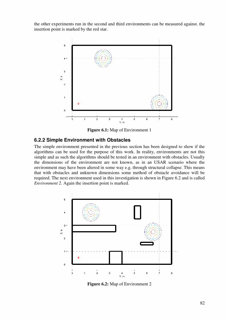
82
the other experiments run in the second and third environments can be measured against. the insertion point is marked by the red star.
Figure 6.1: Map of Environment 1
6.2.2 Simple Environment with Obstacles
The simple environment presented in the previous section has been designed to show if the algorithms can be used for the purpose of this work. In reality, environments are not this simple and as such the algorithms should be tested in an environment with obstacles. Usually the dimensions of the environment are not known, as in an USAR scenario where the environment may have been altered in some way e.g. through structural collapse. This means that with obstacles and unknown dimensions some method of obstacle avoidance will be required. The next environment used in this investigation is shown in Figure 6.2 and is called Environment 2. Again the insertion point is marked.
Figure 6.2: Map of Environment 2
83
It can be clearly seen that there are two targets and that this environment contains obstacles that require detection and avoidance. The insertion point for the robots is (0.5, 0.5), which is located in the lower left corner. With the insertion point located here the robots need to pass through the gap between the two obstacles that confine this starting position. This provides the algorithms with a challenge and shows the benefits and disadvantages of the obstacle avoidance technique that has been implemented. Also it illustrates how the search algorithm accommodates the interruptions caused by the obstacle avoidance.
6.2.3 Complex Environment with Obstacles
The third environment, Environment 3, is larger and more complex than the previous two environments. It represents an office with both small closed off areas and large open spaces. There are seven targets in this environment and a map of it can be seen in Figure 6.3. The insertion point is marked.
Figure 6.3: Map of Environment 3
This environment tests the ability of the algorithms to locate multiple targets and how they operate in a large, irregularly shaped environment with numerous obstacles. The insertion point in this environment is (14, 5).
6.3 Simple Environment Experiments
The first set of experiments will be carried out in the Environment 1. The results from each algorithm are presented. A final comparison is made at the end of the section. To properly gauge how each algorithm performs ten runs are carried out and the average of these runs is calculated to provide the values stated throughout the rest of this chapter. Further data on each of the runs carried out is provided in Appendix C1.
6.3.1 Lawnmower
The first algorithm to be run is the Lawnmower. The advantage of running the Lawnmower first is that it gives a baseline result of what can be achieved in the environment. This is achieved because it gives a structured approach to the search and in this simple environment it can be guaranteed that both targets can be found and that full coverage can be achieved.
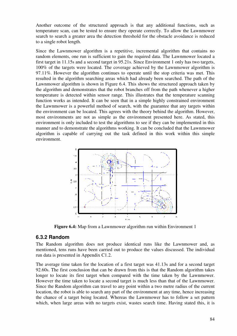
84
Another outcome of the structured approach is that any additional functions, such as temperature scan, can be tested to ensure they operate correctly. To allow the Lawnmower search to search a greater area the detection threshold for the obstacle avoidance is reduced to a single robot length.
Since the Lawnmower algorithm is a repetitive, incremental algorithm that contains no random elements, one run is sufficient to gain the required data. The Lawnmower located a first target in 11.15s and a second target in 95.21s. Since Environment 1 only has two targets, 100% of the targets were located. The coverage achieved by the Lawnmower algorithm is 97.11%. However the algorithm continues to operate until the stop criteria was met. This resulted in the algorithm searching areas which had already been searched. The path of the Lawnmower algorithm is shown in Figure 6.4. This shows the structured approach taken by the algorithm and demonstrates that the robot branches off from the path whenever a higher temperature is detected within sensor range. This illustrates that the temperature scanning function works as intended. It can be seen that in a simple highly constrained environment the Lawnmower is a powerful method of search, with the guarantee that any targets within the environment can be located. This agrees with the theory behind the algorithm. However, most environments are not as simple as the environment presented here. As stated, this environment is only included to test the algorithms to see if they can be implemented in this manner and to demonstrate the algorithms working. It can be concluded that the Lawnmower algorithm is capable of carrying out the task defined in this work within this simple environment.
Figure 6.4: Map from a Lawnmower algorithm run within Environment 1
6.3.2 Random
The Random algorithm does not produce identical runs like the Lawnmower and, as mentioned, tens runs have been carried out to produce the values discussed. The individual run data is presented in Appendix C1.2.
The average time taken for the location of a first target was 41.13s and for a second target 92.60s. The first conclusion that can be drawn from this is that the Random algorithm takes longer to locate its first target when compared with the time taken by the Lawnmower. However the time taken to locate a second target is much less than that of the Lawnmower. Since the Random algorithm can travel to any point within a two metre radius of the current location, the robot is able to search any part of the environment at any time, hence increasing the chance of a target being located. Whereas the Lawnmower has to follow a set pattern which, when large areas with no targets exist, wastes search time. Having stated this, it is
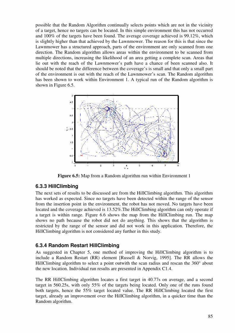
85
possible that the Random Algorithm continually selects points which are not in the vicinity of a target, hence no targets can be located. In this simple environment this has not occurred and 100% of the targets have been found. The average coverage achieved is 99.12%, which is slightly higher than that achieved by the Lawnmower. The reason for this is that since the Lawnmower has a structured approach, parts of the environment are only scanned from one direction. The Random algorithm allows areas within the environment to be scanned from multiple directions, increasing the likelihood of an area getting a complete scan. Areas that lie out with the reach of the Lawnmower’s path have a chance of been scanned also. It should be noted that the difference between the coverage’s is small and that only a small part of the environment is out with the reach of the Lawnmower’s scan. The Random algorithm has been shown to work within Environment 1. A typical run of the Random algorithm is shown in Figure 6.5.
Figure 6.5: Map from a Random algorithm run within Environment 1
6.3.3 HillClimbing
The next sets of results to be discussed are from the HillClimbing algorithm. This algorithm has worked as expected. Since no targets have been detected within the range of the sensor from the insertion point in the environment, the robot has not moved. No targets have been located and the coverage achieved is 13.52%.The HillClimbing algorithm can only operate if a target is within range. Figure 6.6 shows the map from the HillClimbing run. The map shows no path because the robot did not do anything. This shows that the algorithm is restricted by the range of the sensor and did not work in this application. Therefore, the HillClimbing algorithm is not considered any further in this study.
6.3.4 Random Restart HillClimbing
As suggested in Chapter 5, one method of improving the HillClimbing algorithm is to include a Random Restart (RR) element [Russell & Norvig, 1995]. The RR allows the HillClimbing algorithm to select a point outwith the scan radius and rescan the 360° about the new location. Individual run results are presented in Appendix C1.4. The RR HillClimbing algorithm locates a first target in 40.77s on average, and a second target in 560.25s, with only 55% of the targets being located. Only one of the runs found both targets, hence the 55% target located value. The RR HillClimbing located the first target, already an improvement over the HillClimbing algorithm, in a quicker time than the Random algorithm.
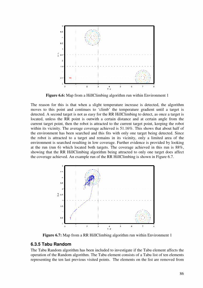
86
Figure 6.6: Map from a HillClimbing algorithm run within Environment 1
The reason for this is that when a slight temperature increase is detected, the algorithm moves to this point and continues to ‘climb’ the temperature gradient until a target is detected. A second target is not as easy for the RR HillClimbing to detect, as once a target is located, unless the RR point is outwith a certain distance and at certain angle from the current target point, then the robot is attracted to the current target point, keeping the robot within its vicinity. The average coverage achieved is 51.16%. This shows that about half of the environment has been searched and this fits with only one target being detected. Since the robot is attracted to a target and remains in its vicinity, only a limited area of the environment is searched resulting in low coverage. Further evidence is provided by looking at the run (run 6) which located both targets. The coverage achieved in this run is 88%, showing that the RR HillClimbing algorithm being attracted to only one target does affect the coverage achieved. An example run of the RR HillClimbing is shown in Figure 6.7.
Figure 6.7: Map from a RR HillClimbing algorithm run within Environment 1
6.3.5 Tabu Random
The Tabu Random algorithm has been included to investigate if the Tabu element affects the operation of the Random algorithm. The Tabu element consists of a Tabu list of ten elements representing the ten last previous visited points. The elements on the list are removed from
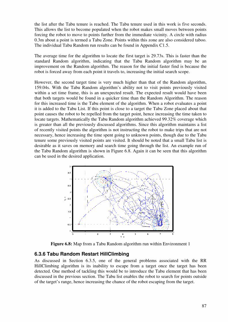
87
the list after the Tabu tenure is reached. The Tabu tenure used in this work is five seconds. This allows the list to become populated when the robot makes small moves between points forcing the robot to move to points further from the immediate vicinity. A circle with radius 0.3m about a point is termed a Tabu Zone. Points within this zone are also considered taboo. The individual Tabu Random run results can be found in Appendix C1.5. The average time for the algorithm to locate the first target is 29.73s. This is faster than the standard Random algorithm, indicating that the Tabu Random algorithm may be an improvement on the Random algorithm. The reason for the initial faster find is because the robot is forced away from each point it travels to, increasing the initial search scope. However, the second target time is very much higher than that of the Random algorithm, 159.04s. With the Tabu Random algorithm’s ability not to visit points previously visited within a set time frame, this is an unexpected result. The expected result would have been that both targets would be found in a quicker time than the Random Algorithm. The reason for this increased time is the Tabu element of the algorithm. When a robot evaluates a point it is added to the Tabu List. If this point is close to a target the Tabu Zone placed about that point causes the robot to be repelled from the target point, hence increasing the time taken to locate targets. Mathematically the Tabu Random algorithm achieved 99.32% coverage which is greater than all the previously discussed algorithms. Since this algorithm maintains a list of recently visited points the algorithm is not instructing the robot to make trips that are not necessary, hence increasing the time spent going to unknown points, though due to the Tabu tenure some previously visited points are visited. It should be noted that a small Tabu list is desirable as it saves on memory and search time going through the list. An example run of the Tabu Random algorithm is shown in Figure 6.8. Again it can be seen that this algorithm can be used in the desired application.
Figure 6.8: Map from a Tabu Random algorithm run within Environment 1
6.3.6 Tabu Random Restart HillClimbing
As discussed in Section 6.3.5, one of the general problems associated with the RR HillClimbing algorithm is its inability to escape from a target once the target has been detected. One method of tackling this would be to introduce the Tabu element that has been discussed in the previous section. The Tabu list enables the robot to search for points outside of the target’s range, hence increasing the chance of the robot escaping from the target.
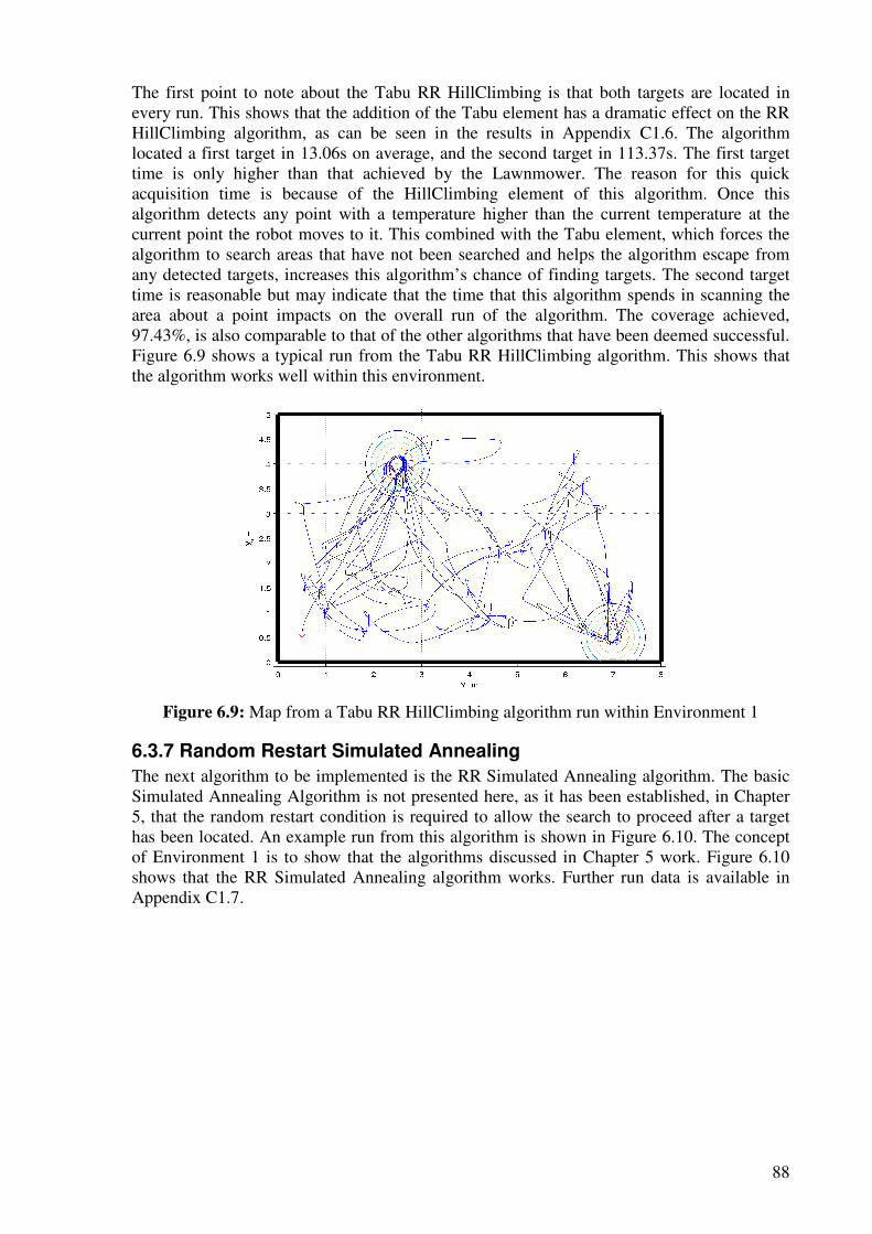
88
The first point to note about the Tabu RR HillClimbing is that both targets are located in every run. This shows that the addition of the Tabu element has a dramatic effect on the RR HillClimbing algorithm, as can be seen in the results in Appendix C1.6. The algorithm located a first target in 13.06s on average, and the second target in 113.37s. The first target time is only higher than that achieved by the Lawnmower. The reason for this quick acquisition time is because of the HillClimbing element of this algorithm. Once this algorithm detects any point with a temperature higher than the current temperature at the current point the robot moves to it. This combined with the Tabu element, which forces the algorithm to search areas that have not been searched and helps the algorithm escape from any detected targets, increases this algorithm’s chance of finding targets. The second target time is reasonable but may indicate that the time that this algorithm spends in scanning the area about a point impacts on the overall run of the algorithm. The coverage achieved, 97.43%, is also comparable to that of the other algorithms that have been deemed successful. Figure 6.9 shows a typical run from the Tabu RR HillClimbing algorithm. This shows that the algorithm works well within this environment.
Figure 6.9: Map from a Tabu RR HillClimbing algorithm run within Environment 1
6.3.7 Random Restart Simulated Annealing
The next algorithm to be implemented is the RR Simulated Annealing algorithm. The basic Simulated Annealing Algorithm is not presented here, as it has been established, in Chapter 5, that the random restart condition is required to allow the search to proceed after a target has been located. An example run from this algorithm is shown in Figure 6.10. The concept of Environment 1 is to show that the algorithms discussed in Chapter 5 work. Figure 6.10 shows that the RR Simulated Annealing algorithm works. Further run data is available in Appendix C1.7.
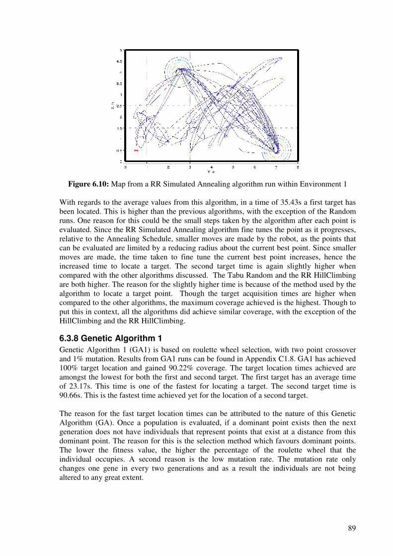
89
Figure 6.10: Map from a RR Simulated Annealing algorithm run within Environment 1
With regards to the average values from this algorithm, in a time of 35.43s a first target has been located. This is higher than the previous algorithms, with the exception of the Random runs. One reason for this could be the small steps taken by the algorithm after each point is evaluated. Since the RR Simulated Annealing algorithm fine tunes the point as it progresses, relative to the Annealing Schedule, smaller moves are made by the robot, as the points that can be evaluated are limited by a reducing radius about the current best point. Since smaller moves are made, the time taken to fine tune the current best point increases, hence the increased time to locate a target. The second target time is again slightly higher when compared with the other algorithms discussed. The Tabu Random and the RR HillClimbing are both higher. The reason for the slightly higher time is because of the method used by the algorithm to locate a target point. Though the target acquisition times are higher when compared to the other algorithms, the maximum coverage achieved is the highest. Though to put this in context, all the algorithms did achieve similar coverage, with the exception of the HillClimbing and the RR HillClimbing.
6.3.8 Genetic Algorithm 1
Genetic Algorithm 1 (GA1) is based on roulette wheel selection, with two point crossover and 1% mutation. Results from GA1 runs can be found in Appendix C1.8. GA1 has achieved 100% target location and gained 90.22% coverage. The target location times achieved are amongst the lowest for both the first and second target. The first target has an average time of 23.17s. This time is one of the fastest for locating a target. The second target time is 90.66s. This is the fastest time achieved yet for the location of a second target. The reason for the fast target location times can be attributed to the nature of this Genetic Algorithm (GA). Once a population is evaluated, if a dominant point exists then the next generation does not have individuals that represent points that exist at a distance from this dominant point. The reason for this is the selection method which favours dominant points. The lower the fitness value, the higher the percentage of the roulette wheel that the individual occupies. A second reason is the low mutation rate. The mutation rate only changes one gene in every two generations and as a result the individuals are not being altered to any great extent.
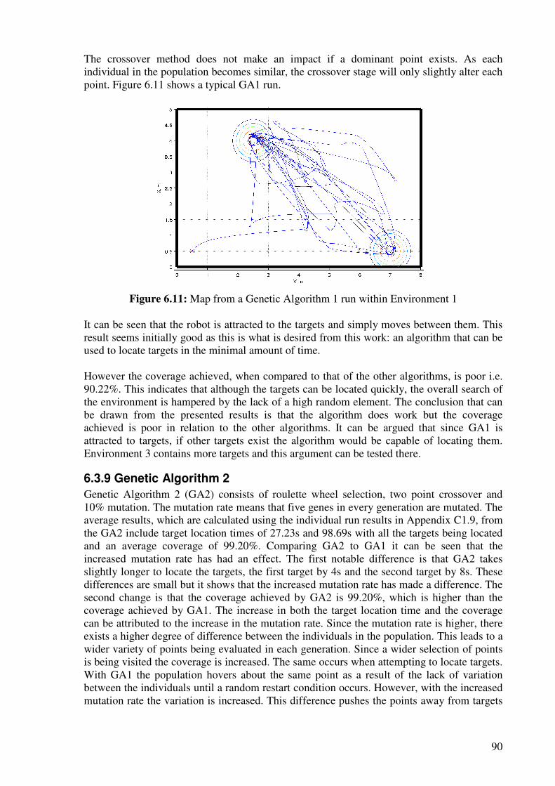
90
The crossover method does not make an impact if a dominant point exists. As each individual in the population becomes similar, the crossover stage will only slightly alter each point. Figure 6.11 shows a typical GA1 run.
Figure 6.11: Map from a Genetic Algorithm 1 run within Environment 1
It can be seen that the robot is attracted to the targets and simply moves between them. This result seems initially good as this is what is desired from this work: an algorithm that can be used to locate targets in the minimal amount of time. However the coverage achieved, when compared to that of the other algorithms, is poor i.e. 90.22%. This indicates that although the targets can be located quickly, the overall search of the environment is hampered by the lack of a high random element. The conclusion that can be drawn from the presented results is that the algorithm does work but the coverage achieved is poor in relation to the other algorithms. It can be argued that since GA1 is attracted to targets, if other targets exist the algorithm would be capable of locating them. Environment 3 contains more targets and this argument can be tested there.
6.3.9 Genetic Algorithm 2
Genetic Algorithm 2 (GA2) consists of roulette wheel selection, two point crossover and 10% mutation. The mutation rate means that five genes in every generation are mutated. The average results, which are calculated using the individual run results in Appendix C1.9, from the GA2 include target location times of 27.23s and 98.69s with all the targets being located and an average coverage of 99.20%. Comparing GA2 to GA1 it can be seen that the increased mutation rate has had an effect. The first notable difference is that GA2 takes slightly longer to locate the targets, the first target by 4s and the second target by 8s. These differences are small but it shows that the increased mutation rate has made a difference. The second change is that the coverage achieved by GA2 is 99.20%, which is higher than the coverage achieved by GA1. The increase in both the target location time and the coverage can be attributed to the increase in the mutation rate. Since the mutation rate is higher, there exists a higher degree of difference between the individuals in the population. This leads to a wider variety of points being evaluated in each generation. Since a wider selection of points is being visited the coverage is increased. The same occurs when attempting to locate targets. With GA1 the population hovers about the same point as a result of the lack of variation between the individuals until a random restart condition occurs. However, with the increased mutation rate the variation is increased. This difference pushes the points away from targets
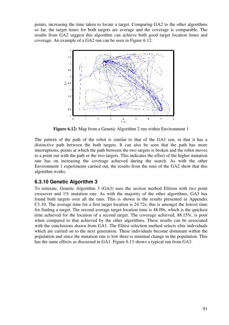
91
points, increasing the time taken to locate a target. Comparing GA2 to the other algorithms so far, the target times for both targets are average and the coverage is comparable. The results from GA2 suggest this algorithm can achieve both good target location times and coverage. An example of a GA2 run can be seen in Figure 6.12.
Figure 6.12: Map from a Genetic Algorithm 2 run within Environment 1
The pattern of the path of the robot is similar to that of the GA1 run, in that it has a distinctive path between the both targets. It can also be seen that the path has more interruptions, points at which the path between the two targets is broken and the robot moves to a point out with the path or the two targets. This indicates the effect of the higher mutation rate has on increasing the coverage achieved during the search. As with the other Environment 1 experiments carried out, the results from the runs of the GA2 show that this algorithm works.
6.3.10 Genetic Algorithm 3
To reiterate, Genetic Algorithm 3 (GA3) uses the section method Elitism with two point crossover and 1% mutation rate. As with the majority of the other algorithms, GA3 has found both targets over all the runs. This is shown in the results presented in Appendix C1.10. The average time for a first target location is 24.72s; this is amongst the lowest time for finding a target. The second average target location time is 48.09s, which is the quickest time achieved for the location of a second target. The coverage achieved, 88.15%, is poor when compared to that achieved by the other algorithms. These results can be associated with the conclusions drawn from GA1. The Elitist selection method selects elite individuals which are carried on to the next generation. These individuals become dominant within the population and since the mutation rate is low there is minimal change in the population. This has the same effects as discussed in GA1. Figure 6.13 shows a typical run from GA3.
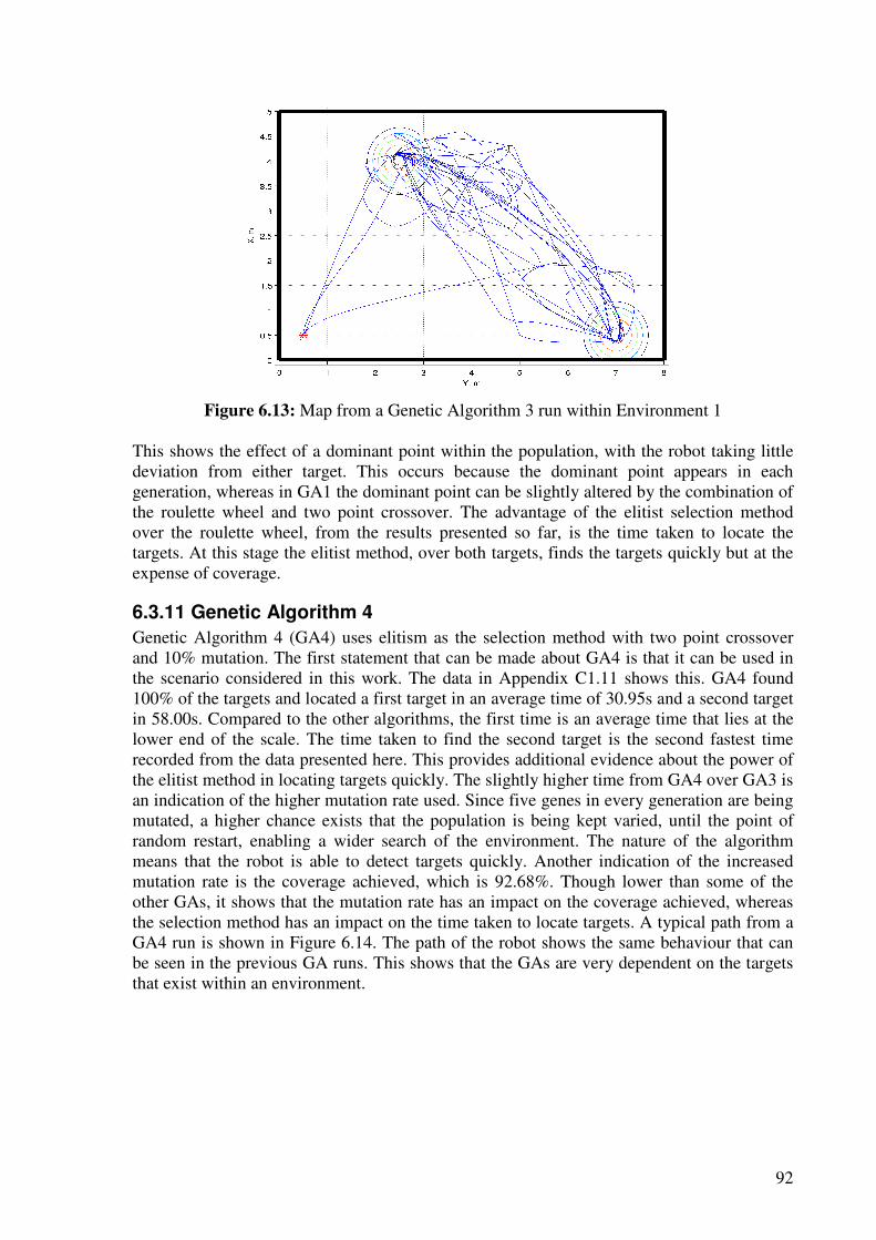
92
Figure 6.13: Map from a Genetic Algorithm 3 run within Environment 1
This shows the effect of a dominant point within the population, with the robot taking little deviation from either target. This occurs because the dominant point appears in each generation, whereas in GA1 the dominant point can be slightly altered by the combination of the roulette wheel and two point crossover. The advantage of the elitist selection method over the roulette wheel, from the results presented so far, is the time taken to locate the targets. At this stage the elitist method, over both targets, finds the targets quickly but at the expense of coverage.
6.3.11 Genetic Algorithm 4
Genetic Algorithm 4 (GA4) uses elitism as the selection method with two point crossover and 10% mutation. The first statement that can be made about GA4 is that it can be used in the scenario considered in this work. The data in Appendix C1.11 shows this. GA4 found 100% of the targets and located a first target in an average time of 30.95s and a second target in 58.00s. Compared to the other algorithms, the first time is an average time that lies at the lower end of the scale. The time taken to find the second target is the second fastest time recorded from the data presented here. This provides additional evidence about the power of the elitist method in locating targets quickly. The slightly higher time from GA4 over GA3 is an indication of the higher mutation rate used. Since five genes in every generation are being mutated, a higher chance exists that the population is being kept varied, until the point of random restart, enabling a wider search of the environment. The nature of the algorithm means that the robot is able to detect targets quickly. Another indication of the increased mutation rate is the coverage achieved, which is 92.68%. Though lower than some of the other GAs, it shows that the mutation rate has an impact on the coverage achieved, whereas the selection method has an impact on the time taken to locate targets. A typical path from a GA4 run is shown in Figure 6.14. The path of the robot shows the same behaviour that can be seen in the previous GA runs. This shows that the GAs are very dependent on the targets that exist within an environment.
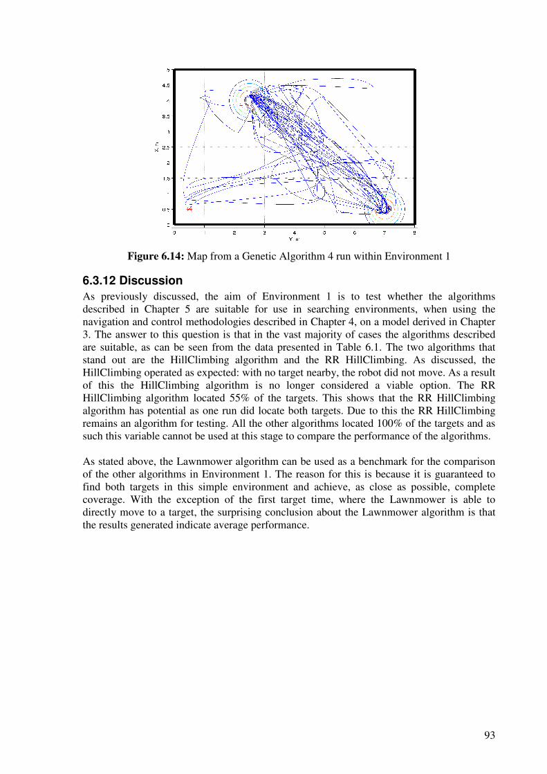
93
Figure 6.14: Map from a Genetic Algorithm 4 run within Environment 1
6.3.12 Discussion
As previously discussed, the aim of Environment 1 is to test whether the algorithms described in Chapter 5 are suitable for use in searching environments, when using the navigation and control methodologies described in Chapter 4, on a model derived in Chapter 3. The answer to this question is that in the vast majority of cases the algorithms described are suitable, as can be seen from the data presented in Table 6.1. The two algorithms that stand out are the HillClimbing algorithm and the RR HillClimbing. As discussed, the HillClimbing operated as expected: with no target nearby, the robot did not move. As a result of this the HillClimbing algorithm is no longer considered a viable option. The RR HillClimbing algorithm located 55% of the targets. This shows that the RR HillClimbing algorithm has potential as one run did locate both targets. Due to this the RR HillClimbing remains an algorithm for testing. All the other algorithms located 100% of the targets and as such this variable cannot be used at this stage to compare the performance of the algorithms. As stated above, the Lawnmower algorithm can be used as a benchmark for the comparison of the other algorithms in Environment 1. The reason for this is because it is guaranteed to find both targets in this simple environment and achieve, as close as possible, complete coverage. With the exception of the first target time, where the Lawnmower is able to directly move to a target, the surprising conclusion about the Lawnmower algorithm is that the results generated indicate average performance.
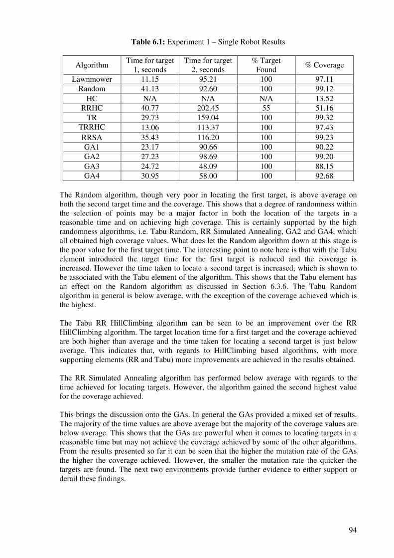
94
Table 6.1: Experiment 1 – Single Robot Results
Algorithm Time for target
1, seconds Time for target
2, seconds % Target
Found % Coverage
Lawnmower 11.15 95.21 100 97.11 Random 41.13 92.60 100 99.12
HC N/A N/A N/A 13.52 RRHC 40.77 202.45 55 51.16
TR 29.73 159.04 100 99.32 TRRHC 13.06 113.37 100 97.43 RRSA 35.43 116.20 100 99.23 GA1 23.17 90.66 100 90.22 GA2 27.23 98.69 100 99.20 GA3 24.72 48.09 100 88.15 GA4 30.95 58.00 100 92.68
The Random algorithm, though very poor in locating the first target, is above average on both the second target time and the coverage. This shows that a degree of randomness within the selection of points may be a major factor in both the location of the targets in a reasonable time and on achieving high coverage. This is certainly supported by the high randomness algorithms, i.e. Tabu Random, RR Simulated Annealing, GA2 and GA4, which all obtained high coverage values. What does let the Random algorithm down at this stage is the poor value for the first target time. The interesting point to note here is that with the Tabu element introduced the target time for the first target is reduced and the coverage is increased. However the time taken to locate a second target is increased, which is shown to be associated with the Tabu element of the algorithm. This shows that the Tabu element has an effect on the Random algorithm as discussed in Section 6.3.6. The Tabu Random algorithm in general is below average, with the exception of the coverage achieved which is the highest. The Tabu RR HillClimbing algorithm can be seen to be an improvement over the RR HillClimbing algorithm. The target location time for a first target and the coverage achieved are both higher than average and the time taken for locating a second target is just below average. This indicates that, with regards to HillClimbing based algorithms, with more supporting elements (RR and Tabu) more improvements are achieved in the results obtained. The RR Simulated Annealing algorithm has performed below average with regards to the time achieved for locating targets. However, the algorithm gained the second highest value for the coverage achieved. This brings the discussion onto the GAs. In general the GAs provided a mixed set of results. The majority of the time values are above average but the majority of the coverage values are below average. This shows that the GAs are powerful when it comes to locating targets in a reasonable time but may not achieve the coverage achieved by some of the other algorithms. From the results presented so far it can be seen that the higher the mutation rate of the GAs the higher the coverage achieved. However, the smaller the mutation rate the quicker the targets are found. The next two environments provide further evidence to either support or derail these findings.
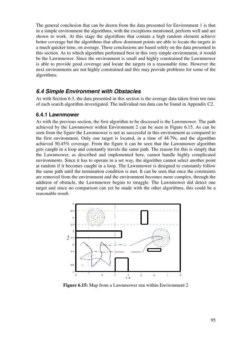
95
The general conclusion that can be drawn from the data presented for Environment 1 is that in a simple environment the algorithms, with the exceptions mentioned, perform well and are shown to work. At this stage the algorithms that contain a high random element achieve better coverage but the algorithms that allow dominant points are able to locate the targets in a much quicker time, on average. These conclusions are based solely on the data presented in this section. As to which algorithm performed best in this very simple environment, it would be the Lawnmower. Since the environment is small and highly constrained the Lawnmower is able to provide good coverage and locate the targets in a reasonable time. However the next environments are not highly constrained and this may provide problems for some of the algorithms.
6.4 Simple Environment with Obstacles
As with Section 6.3, the data presented in this section is the average data taken from ten runs of each search algorithm investigated. The individual run data can be found in Appendix C2.
6.4.1 Lawnmower
As with the previous section, the first algorithm to be discussed is the Lawnmower. The path achieved by the Lawnmower within Environment 2 can be seen in Figure 6.15. As can be seen from the figure the Lawnmower is not as successful in this environment as compared to the first environment. Only one target is located, in a time of 48.79s, and the algorithm achieved 50.45% coverage. From the figure it can be seen that the Lawnmower algorithm gets caught in a loop and constantly travels the same path. The reason for this is simply that the Lawnmower, as described and implemented here, cannot handle highly complicated environments. Since it has to operate in a set way, the algorithm cannot select another point at random if it becomes caught in a loop. The Lawnmower is designed to constantly follow the same path until the termination condition is met. It can be seen that once the constraints are removed from the environment and the environment becomes more complex, through the addition of obstacle, the Lawnmower begins to struggle. The Lawnmower did detect one target and since no comparison can yet be made with the other algorithms, this could be a reasonable result.
Figure 6.15: Map from a Lawnmower run within Environment 2
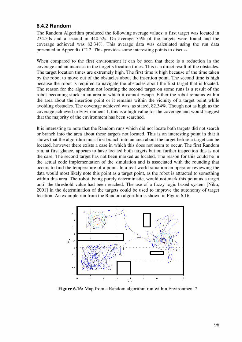
96
6.4.2 Random
The Random Algorithm produced the following average values: a first target was located in 234.50s and a second in 440.52s. On average 75% of the targets were found and the coverage achieved was 82.34%. This average data was calculated using the run data presented in Appendix C2.2. This provides some interesting points to discuss. When compared to the first environment it can be seen that there is a reduction in the coverage and an increase in the target’s location times. This is a direct result of the obstacles. The target location times are extremely high. The first time is high because of the time taken by the robot to move out of the obstacles about the insertion point. The second time is high because the robot is required to navigate the obstacles about the first target that is located. The reason for the algorithm not locating the second target on some runs is a result of the robot becoming stuck in an area in which it cannot escape. Either the robot remains within the area about the insertion point or it remains within the vicinity of a target point while avoiding obstacles. The coverage achieved was, as stated, 82.34%. Though not as high as the coverage achieved in Environment 1, this is a high value for the coverage and would suggest that the majority of the environment has been searched. It is interesting to note that the Random runs which did not locate both targets did not search or branch into the area about these targets not located. This is an interesting point in that it shows that the algorithm must first branch into an area about the target before a target can be located, however there exists a case in which this does not seem to occur. The first Random run, at first glance, appears to have located both targets but on further inspection this is not the case. The second target has not been marked as located. The reason for this could be in the actual code implementation of the simulation and is associated with the rounding that occurs to find the temperature of a point. In a real world situation an operator reviewing the data would most likely note this point as a target point, as the robot is attracted to something within this area. The robot, being purely deterministic, would not mark this point as a target until the threshold value had been reached. The use of a fuzzy logic based system [Niku, 2001] in the determination of the targets could be used to improve the autonomy of target location. An example run from the Random algorithm is shown in Figure 6.16.
Figure 6.16: Map from a Random algorithm run within Environment 2
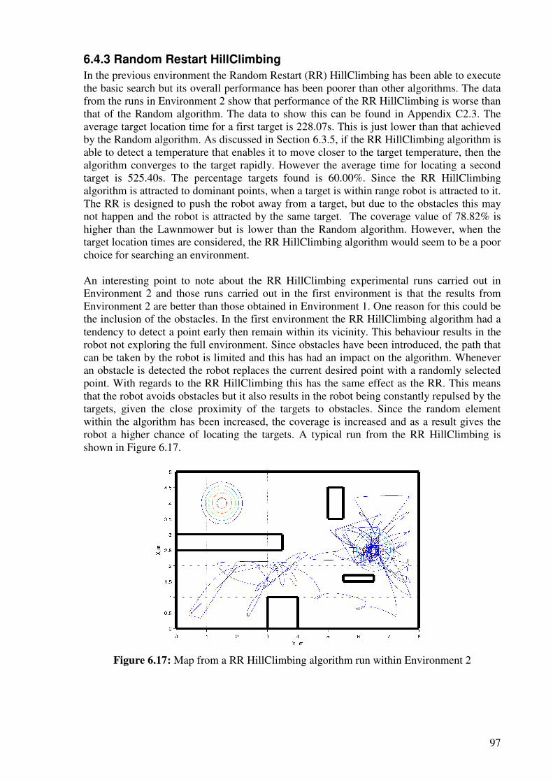
97
6.4.3 Random Restart HillClimbing
In the previous environment the Random Restart (RR) HillClimbing has been able to execute the basic search but its overall performance has been poorer than other algorithms. The data from the runs in Environment 2 show that performance of the RR HillClimbing is worse than that of the Random algorithm. The data to show this can be found in Appendix C2.3. The average target location time for a first target is 228.07s. This is just lower than that achieved by the Random algorithm. As discussed in Section 6.3.5, if the RR HillClimbing algorithm is able to detect a temperature that enables it to move closer to the target temperature, then the algorithm converges to the target rapidly. However the average time for locating a second target is 525.40s. The percentage targets found is 60.00%. Since the RR HillClimbing algorithm is attracted to dominant points, when a target is within range robot is attracted to it. The RR is designed to push the robot away from a target, but due to the obstacles this may not happen and the robot is attracted by the same target. The coverage value of 78.82% is higher than the Lawnmower but is lower than the Random algorithm. However, when the target location times are considered, the RR HillClimbing algorithm would seem to be a poor choice for searching an environment. An interesting point to note about the RR HillClimbing experimental runs carried out in Environment 2 and those runs carried out in the first environment is that the results from Environment 2 are better than those obtained in Environment 1. One reason for this could be the inclusion of the obstacles. In the first environment the RR HillClimbing algorithm had a tendency to detect a point early then remain within its vicinity. This behaviour results in the robot not exploring the full environment. Since obstacles have been introduced, the path that can be taken by the robot is limited and this has had an impact on the algorithm. Whenever an obstacle is detected the robot replaces the current desired point with a randomly selected point. With regards to the RR HillClimbing this has the same effect as the RR. This means that the robot avoids obstacles but it also results in the robot being constantly repulsed by the targets, given the close proximity of the targets to obstacles. Since the random element within the algorithm has been increased, the coverage is increased and as a result gives the robot a higher chance of locating the targets. A typical run from the RR HillClimbing is shown in Figure 6.17.
Figure 6.17: Map from a RR HillClimbing algorithm run within Environment 2
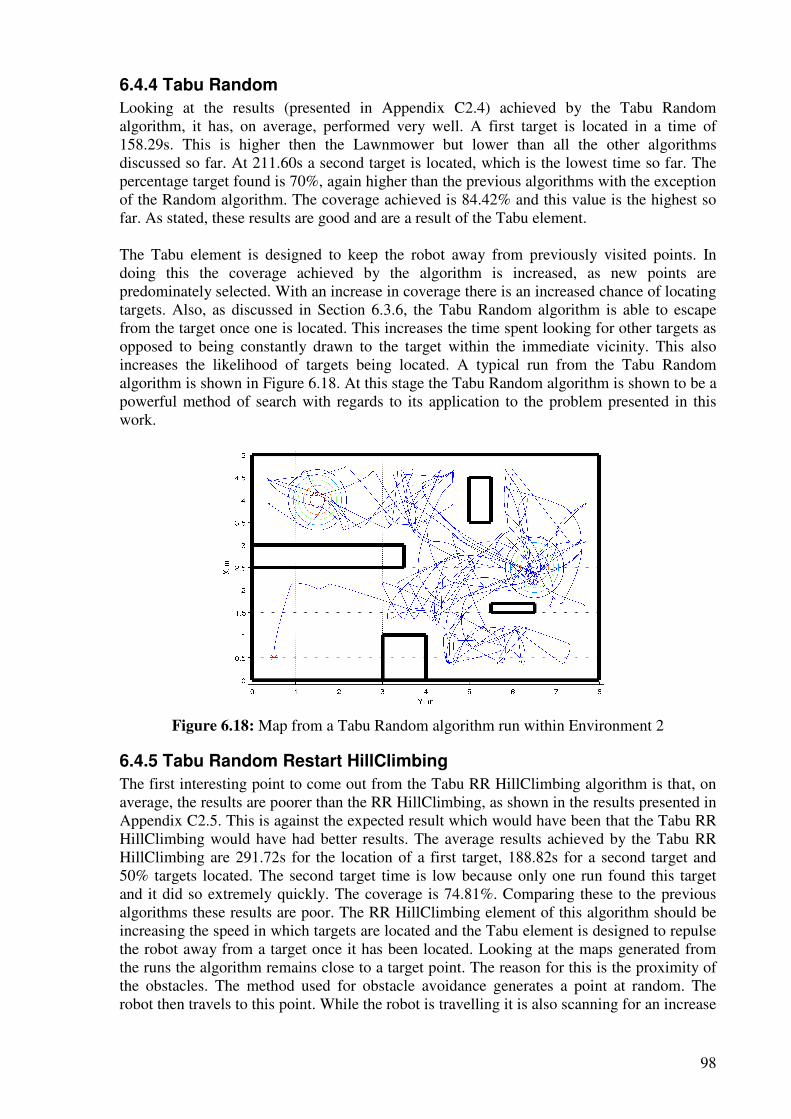
98
6.4.4 Tabu Random
Looking at the results (presented in Appendix C2.4) achieved by the Tabu Random algorithm, it has, on average, performed very well. A first target is located in a time of 158.29s. This is higher then the Lawnmower but lower than all the other algorithms discussed so far. At 211.60s a second target is located, which is the lowest time so far. The percentage target found is 70%, again higher than the previous algorithms with the exception of the Random algorithm. The coverage achieved is 84.42% and this value is the highest so far. As stated, these results are good and are a result of the Tabu element. The Tabu element is designed to keep the robot away from previously visited points. In doing this the coverage achieved by the algorithm is increased, as new points are predominately selected. With an increase in coverage there is an increased chance of locating targets. Also, as discussed in Section 6.3.6, the Tabu Random algorithm is able to escape from the target once one is located. This increases the time spent looking for other targets as opposed to being constantly drawn to the target within the immediate vicinity. This also increases the likelihood of targets being located. A typical run from the Tabu Random algorithm is shown in Figure 6.18. At this stage the Tabu Random algorithm is shown to be a powerful method of search with regards to its application to the problem presented in this work.
Figure 6.18: Map from a Tabu Random algorithm run within Environment 2
6.4.5 Tabu Random Restart HillClimbing
The first interesting point to come out from the Tabu RR HillClimbing algorithm is that, on average, the results are poorer than the RR HillClimbing, as shown in the results presented in Appendix C2.5. This is against the expected result which would have been that the Tabu RR HillClimbing would have had better results. The average results achieved by the Tabu RR HillClimbing are 291.72s for the location of a first target, 188.82s for a second target and 50% targets located. The second target time is low because only one run found this target and it did so extremely quickly. The coverage is 74.81%. Comparing these to the previous algorithms these results are poor. The RR HillClimbing element of this algorithm should be increasing the speed in which targets are located and the Tabu element is designed to repulse the robot away from a target once it has been located. Looking at the maps generated from the runs the algorithm remains close to a target point. The reason for this is the proximity of the obstacles. The method used for obstacle avoidance generates a point at random. The robot then travels to this point. While the robot is travelling it is also scanning for an increase
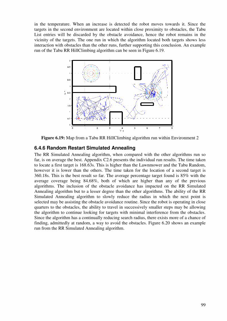
99
in the temperature. When an increase is detected the robot moves towards it. Since the targets in the second environment are located within close proximity to obstacles, the Tabu List entries will be discarded by the obstacle avoidance, hence the robot remains in the vicinity of the targets. The one run in which the algorithm located both targets shows less interaction with obstacles than the other runs, further supporting this conclusion. An example run of the Tabu RR HillClimbing algorithm can be seen in Figure 6.19.
Figure 6.19: Map from a Tabu RR HillClimbing algorithm run within Environment 2
6.4.6 Random Restart Simulated Annealing
The RR Simulated Annealing algorithm, when compared with the other algorithms run so far, is on average the best. Appendix C2.6 presents the individual run results. The time taken to locate a first target is 168.63s. This is higher than the Lawnmower and the Tabu Random, however it is lower than the others. The time taken for the location of a second target is 360.18s. This is the best result so far. The average percentage target found is 85% with the average coverage being 84.68%, both of which are higher than any of the previous algorithms. The inclusion of the obstacle avoidance has impacted on the RR Simulated Annealing algorithm but to a lesser degree than the other algorithms. The ability of the RR Simulated Annealing algorithm to slowly reduce the radius in which the next point is selected may be assisting the obstacle avoidance routine. Since the robot is operating in close quarters to the obstacles, the ability to travel in successively smaller steps may be allowing the algorithm to continue looking for targets with minimal interference from the obstacles. Since the algorithm has a continually reducing search radius, there exists more of a chance of finding, admittedly at random, a way to avoid the obstacles. Figure 6.20 shows an example run from the RR Simulated Annealing algorithm.
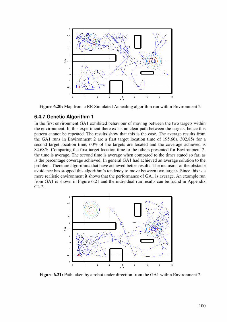
100
Figure 6.20: Map from a RR Simulated Annealing algorithm run within Environment 2
6.4.7 Genetic Algorithm 1
In the first environment GA1 exhibited behaviour of moving between the two targets within the environment. In this experiment there exists no clear path between the targets, hence this pattern cannot be repeated. The results show that this is the case. The average results from the GA1 runs in Environment 2 are a first target location time of 195.66s, 302.85s for a second target location time, 60% of the targets are located and the coverage achieved is 84.68%. Comparing the first target location time to the others presented for Environment 2, the time is average. The second time is average when compared to the times stated so far, as is the percentage coverage achieved. In general GA1 had achieved an average solution to the problem. There are algorithms that have achieved better results. The inclusion of the obstacle avoidance has stopped this algorithm’s tendency to move between two targets. Since this is a more realistic environment it shows that the performance of GA1 is average. An example run from GA1 is shown in Figure 6.21 and the individual run results can be found in Appendix C2.7.
Figure 6.21: Path taken by a robot under direction from the GA1 within Environment 2
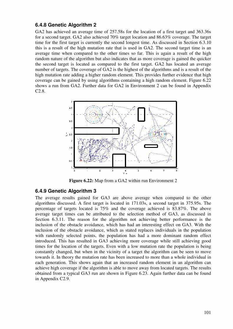
101
6.4.8 Genetic Algorithm 2
GA2 has achieved an average time of 257.58s for the location of a first target and 363.36s for a second target. GA2 also achieved 70% target location and 86.63% coverage. The target time for the first target is currently the second longest time. As discussed in Section 6.3.10 this is a result of the high mutation rate that is used in GA2. The second target time is an average time when compared to the other times so far. This is again a result of the high random nature of the algorithm but also indicates that as more coverage is gained the quicker the second target is located as compared to the first target. GA2 has located an average number of targets. The coverage of GA2 is the highest of the algorithms and is a result of the high mutation rate adding a higher random element. This provides further evidence that high coverage can be gained by using algorithms containing a high random element. Figure 6.22 shows a run from GA2. Further data for GA2 in Environment 2 can be found in Appendix C2.8.
Figure 6.22: Map from a GA2 within run Environment 2
6.4.9 Genetic Algorithm 3
The average results gained for GA3 are above average when compared to the other algorithms discussed. A first target is located in 171.03s, a second target in 375.95s. The percentage of targets located is 75% and the coverage achieved is 83.87%. The above average target times can be attributed to the selection method of GA3, as discussed in Section 6.3.11. The reason for the algorithm not achieving better performance is the inclusion of the obstacle avoidance, which has had an interesting effect on GA3. With the inclusion of the obstacle avoidance, which as stated replaces individuals in the population with randomly selected points, the population has had a more dominant random effect introduced. This has resulted in GA3 achieving more coverage while still achieving good times for the location of the targets. Even with a low mutation rate the population is being constantly changed, but when in the vicinity of a target the algorithm can be seen to move towards it. In theory the mutation rate has been increased to more than a whole individual in each generation. This shows again that an increased random element in an algorithm can achieve high coverage if the algorithm is able to move away from located targets. The results obtained from a typical GA3 run are shown in Figure 6.23. Again further data can be found in Appendix C2.9.
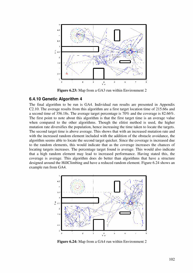
102
Figure 6.23: Map from a GA3 run within Environment 2
6.4.10 Genetic Algorithm 4
The final algorithm to be run is GA4. Individual run results are presented in Appendix C2.10. The average results from this algorithm are a first target location time of 215.66s and a second time of 356.18s. The average target percentage is 70% and the coverage is 82.66%. The first point to note about this algorithm is that the first target time is an average value when compared to the other algorithms. Though the elitist method is used, the higher mutation rate diversifies the population, hence increasing the time taken to locate the targets. The second target time is above average. This shows that with an increased mutation rate and with the increased random element included with the addition of the obstacle avoidance, the algorithm seems able to locate the second target quicker. Since the coverage is increased due to the random elements, this would indicate that as the coverage increases the chances of locating targets increases. The percentage target found is average. This would also indicate that a high random element may lead to increased performance. Having stated this, the coverage is average. This algorithm does do better than algorithms that have a structure designed around the HillClimbing and have a reduced random element. Figure 6.24 shows an example run from GA4.
Figure 6.24: Map from a GA4 run within Environment 2
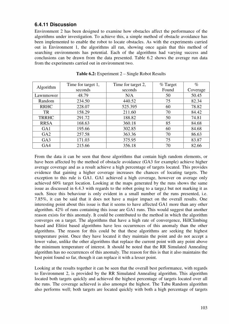
103
6.4.11 Discussion
Environment 2 has been designed to examine how obstacles affect the performance of the algorithms under investigation. To achieve this, a simple method of obstacle avoidance has been implemented to enable the robot to locate obstacles. As with the experiments carried out in Environment 1, the algorithms all ran, showing once again that this method of searching environments has potential. Each of the algorithms had varying success and conclusions can be drawn from the data presented. Table 6.2 shows the average run data from the experiments carried out in environment two.
Table 6.2: Experiment 2 – Single Robot Results
Algorithm Time for target 1,
seconds Time for target 2,
seconds % Target
Found %
Coverage Lawnmower 48.79 N/A 50 50.45
Random 234.50 440.52 75 82.34 RRHC 228.07 525.395 60 78.82
TR 158.29 211.60 70 84.42 TRRHC 291.72 188.82 50 74.81 RRSA 168.63 360.18 85 84.68 GA1 195.66 302.85 60 84.68 GA2 257.58 363.36 70 86.63 GA3 171.03 375.95 75 83.87 GA4 215.66 356.18 70 82.66
From the data it can be seen that those algorithms that contain high random elements, or have been affected by the method of obstacle avoidance (GA3 for example) achieve higher average coverage and as a result achieve a high percentage of targets located. This provides evidence that gaining a higher coverage increases the chances of locating targets. The exception to this rule is GA1. GA1 achieved a high coverage, however on average only achieved 60% target location. Looking at the maps generated by the runs shows the same issue as discussed in 6.4.3 with regards to the robot going to a targe,t but not marking it as such. Since this behaviour is only evident in a small number of the runs presented, i.e. 7.85%, it can be said that it does not have a major impact on the overall results. One interesting point about this issue is that it seems to have affected GA1 more than any other algorithm. 42% of runs containing this issue are GA1 runs. This would suggest that another reason exists for this anomaly. It could be contributed to the method in which the algorithm converges on a target. The algorithms that have a high rate of convergence, HillClimbing based and Elitist based algorithms have less occurrences of this anomaly than the other algorithms. The reason for this could be that these algorithms are seeking the highest temperature point. Once they have located it they maintain the point and do not accept a lower value, unlike the other algorithms that replace the current point with any point above the minimum temperature of interest. It should be noted that the RR Simulated Annealing algorithm has no occurrences of this anomaly. The reason for this is that it also maintains the best point found so far, though it can replace it with a lesser point. Looking at the results together it can be seen that the overall best performance, with regards to Environment 2, is provided by the RR Simulated Annealing algorithm. This algorithm located both targets quickly and achieved the highest percentage of targets located over all the runs. The coverage achieved is also amongst the highest. The Tabu Random algorithm also performs well; both targets are located quickly with both a high percentage of targets
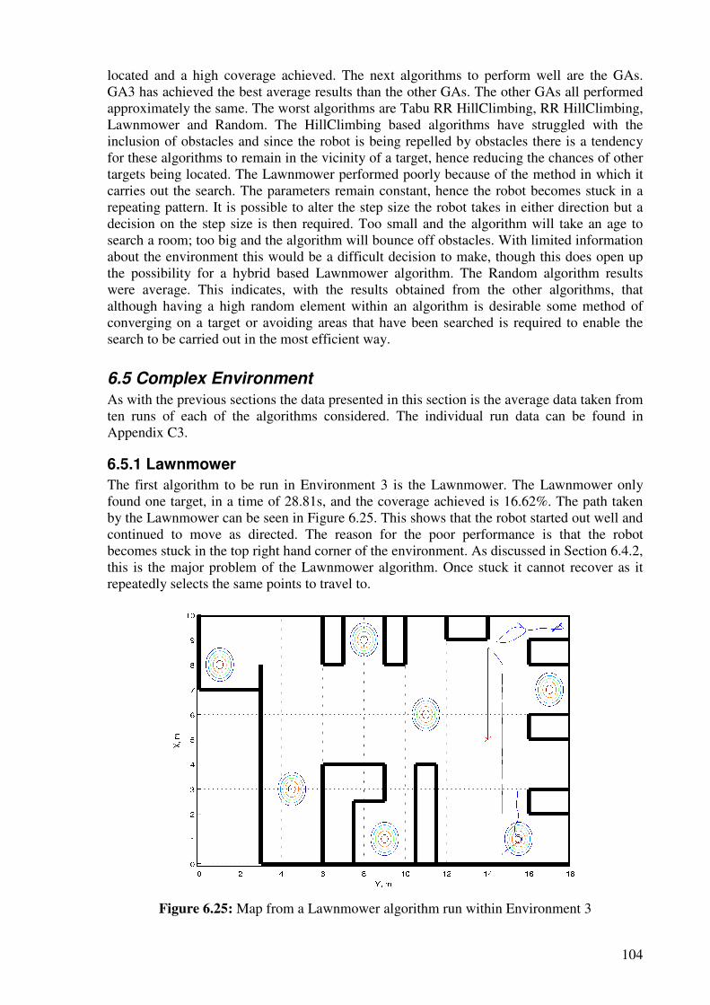
104
located and a high coverage achieved. The next algorithms to perform well are the GAs. GA3 has achieved the best average results than the other GAs. The other GAs all performed approximately the same. The worst algorithms are Tabu RR HillClimbing, RR HillClimbing, Lawnmower and Random. The HillClimbing based algorithms have struggled with the inclusion of obstacles and since the robot is being repelled by obstacles there is a tendency for these algorithms to remain in the vicinity of a target, hence reducing the chances of other targets being located. The Lawnmower performed poorly because of the method in which it carries out the search. The parameters remain constant, hence the robot becomes stuck in a repeating pattern. It is possible to alter the step size the robot takes in either direction but a decision on the step size is then required. Too small and the algorithm will take an age to search a room; too big and the algorithm will bounce off obstacles. With limited information about the environment this would be a difficult decision to make, though this does open up the possibility for a hybrid based Lawnmower algorithm. The Random algorithm results were average. This indicates, with the results obtained from the other algorithms, that although having a high random element within an algorithm is desirable some method of converging on a target or avoiding areas that have been searched is required to enable the search to be carried out in the most efficient way.
6.5 Complex Environment
As with the previous sections the data presented in this section is the average data taken from ten runs of each of the algorithms considered. The individual run data can be found in Appendix C3.
6.5.1 Lawnmower
The first algorithm to be run in Environment 3 is the Lawnmower. The Lawnmower only found one target, in a time of 28.81s, and the coverage achieved is 16.62%. The path taken by the Lawnmower can be seen in Figure 6.25. This shows that the robot started out well and continued to move as directed. The reason for the poor performance is that the robot becomes stuck in the top right hand corner of the environment. As discussed in Section 6.4.2, this is the major problem of the Lawnmower algorithm. Once stuck it cannot recover as it repeatedly selects the same points to travel to.
Figure 6.25: Map from a Lawnmower algorithm run within Environment 3
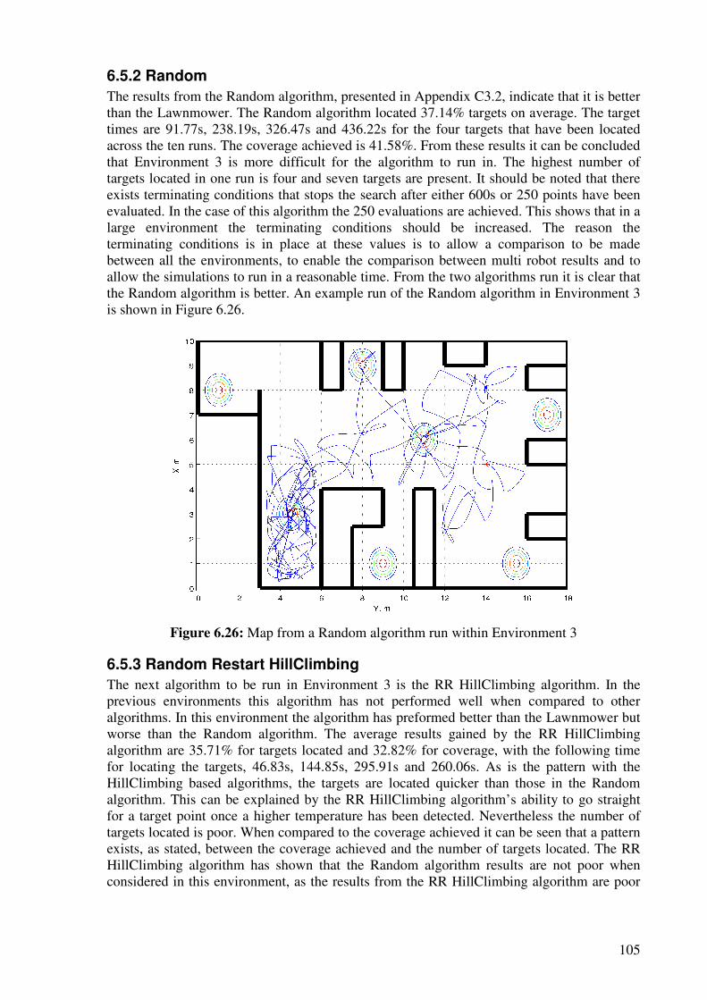
105
6.5.2 Random
The results from the Random algorithm, presented in Appendix C3.2, indicate that it is better than the Lawnmower. The Random algorithm located 37.14% targets on average. The target times are 91.77s, 238.19s, 326.47s and 436.22s for the four targets that have been located across the ten runs. The coverage achieved is 41.58%. From these results it can be concluded that Environment 3 is more difficult for the algorithm to run in. The highest number of targets located in one run is four and seven targets are present. It should be noted that there exists terminating conditions that stops the search after either 600s or 250 points have been evaluated. In the case of this algorithm the 250 evaluations are achieved. This shows that in a large environment the terminating conditions should be increased. The reason the terminating conditions is in place at these values is to allow a comparison to be made between all the environments, to enable the comparison between multi robot results and to allow the simulations to run in a reasonable time. From the two algorithms run it is clear that the Random algorithm is better. An example run of the Random algorithm in Environment 3 is shown in Figure 6.26.
Figure 6.26: Map from a Random algorithm run within Environment 3
6.5.3 Random Restart HillClimbing
The next algorithm to be run in Environment 3 is the RR HillClimbing algorithm. In the previous environments this algorithm has not performed well when compared to other algorithms. In this environment the algorithm has preformed better than the Lawnmower but worse than the Random algorithm. The average results gained by the RR HillClimbing algorithm are 35.71% for targets located and 32.82% for coverage, with the following time for locating the targets, 46.83s, 144.85s, 295.91s and 260.06s. As is the pattern with the HillClimbing based algorithms, the targets are located quicker than those in the Random algorithm. This can be explained by the RR HillClimbing algorithm’s ability to go straight for a target point once a higher temperature has been detected. Nevertheless the number of targets located is poor. When compared to the coverage achieved it can be seen that a pattern exists, as stated, between the coverage achieved and the number of targets located. The RR HillClimbing algorithm has shown that the Random algorithm results are not poor when considered in this environment, as the results from the RR HillClimbing algorithm are poor
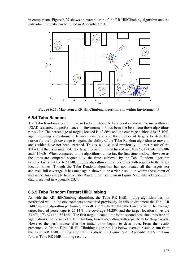
106
in comparison. Figure 6.27 shows an example run of the RR HillClimbing algorithm and the individual run data can be found in Appendix C3.3.
Figure 6.27: Map from a RR HillClimbing algorithm run within Environment 3
6.5.4 Tabu Random
The Tabu Random algorithm has so far been shown to be a good candidate for use within an USAR scenario. Its performance in Environment 3 has been the best from those algorithms run so far. The percentage of targets located is 42.86% and the coverage achieved is 45.10%, again showing a relationship between coverage and the number of targets located. The reason for the high coverage is, again, the ability of the Tabu Random algorithm to move to areas which have not been searched. This is, as discussed previously, a direct result of the Tabu List that is maintained. The target located times achieved are, 43.23s, 194.84s, 338.88s and 415.63s. When compared to the algorithms run so far, the first time is slow. However as the times are compared sequentially, the times achieved by the Tabu Random algorithm become faster but the RR HillClimbing algorithm still outperforms with regards to the target location times. Though the Tabu Random algorithm has not located all the targets nor achieved full coverage, it has once again shown to be a viable solution within the context of this work. An example from a Tabu Random run is shown in Figure 6.28 with additional run data presented in Appendix C3.4.
6.5.5 Tabu Random Restart HillClimbing
As with the RR HillClimbing algorithm, the Tabu RR HillClimbing algorithm has not performed well in the environments considered previously. In this environment the Tabu RR HillClimbing algorithm performed, overall, slightly better than the Lawnmower. The average target located percentage is 27.14%, the coverage 34.20% and the target location times are 33.47s, 173.69s and 324.45s. The first target located time is the second best time thus far and again shows the power of a HillClimbing based algorithm with regards to locating targets. However the performance after the initial point begins to deteriorate. From the results presented so far the Tabu RR HillClimbing algorithm is a below average result. A run from the Tabu RR HillClimbing algorithm is shown in Figure 6.29. Appendix C3.5 contains further Tabu RR HillClimbing results.
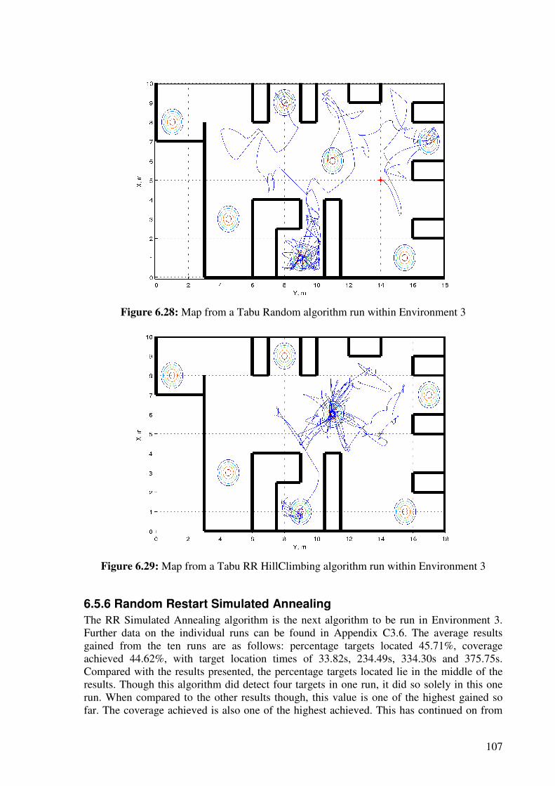
107
Figure 6.28: Map from a Tabu Random algorithm run within Environment 3
Figure 6.29: Map from a Tabu RR HillClimbing algorithm run within Environment 3
6.5.6 Random Restart Simulated Annealing
The RR Simulated Annealing algorithm is the next algorithm to be run in Environment 3. Further data on the individual runs can be found in Appendix C3.6. The average results gained from the ten runs are as follows: percentage targets located 45.71%, coverage achieved 44.62%, with target location times of 33.82s, 234.49s, 334.30s and 375.75s. Compared with the results presented, the percentage targets located lie in the middle of the results. Though this algorithm did detect four targets in one run, it did so solely in this one run. When compared to the other results though, this value is one of the highest gained so far. The coverage achieved is also one of the highest achieved. This has continued on from
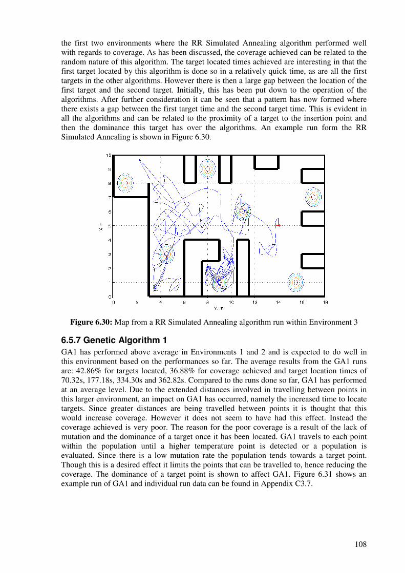
108
the first two environments where the RR Simulated Annealing algorithm performed well with regards to coverage. As has been discussed, the coverage achieved can be related to the random nature of this algorithm. The target located times achieved are interesting in that the first target located by this algorithm is done so in a relatively quick time, as are all the first targets in the other algorithms. However there is then a large gap between the location of the first target and the second target. Initially, this has been put down to the operation of the algorithms. After further consideration it can be seen that a pattern has now formed where there exists a gap between the first target time and the second target time. This is evident in all the algorithms and can be related to the proximity of a target to the insertion point and then the dominance this target has over the algorithms. An example run form the RR Simulated Annealing is shown in Figure 6.30.
Figure 6.30: Map from a RR Simulated Annealing algorithm run within Environment 3
6.5.7 Genetic Algorithm 1
GA1 has performed above average in Environments 1 and 2 and is expected to do well in this environment based on the performances so far. The average results from the GA1 runs are: 42.86% for targets located, 36.88% for coverage achieved and target location times of 70.32s, 177.18s, 334.30s and 362.82s. Compared to the runs done so far, GA1 has performed at an average level. Due to the extended distances involved in travelling between points in this larger environment, an impact on GA1 has occurred, namely the increased time to locate targets. Since greater distances are being travelled between points it is thought that this would increase coverage. However it does not seem to have had this effect. Instead the coverage achieved is very poor. The reason for the poor coverage is a result of the lack of mutation and the dominance of a target once it has been located. GA1 travels to each point within the population until a higher temperature point is detected or a population is evaluated. Since there is a low mutation rate the population tends towards a target point. Though this is a desired effect it limits the points that can be travelled to, hence reducing the coverage. The dominance of a target point is shown to affect GA1. Figure 6.31 shows an example run of GA1 and individual run data can be found in Appendix C3.7.
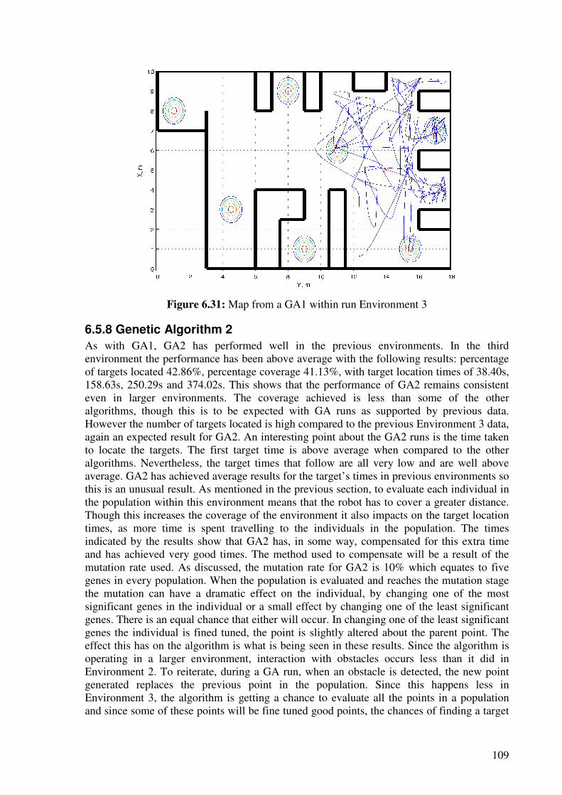
109
Figure 6.31: Map from a GA1 within run Environment 3
6.5.8 Genetic Algorithm 2
As with GA1, GA2 has performed well in the previous environments. In the third environment the performance has been above average with the following results: percentage of targets located 42.86%, percentage coverage 41.13%, with target location times of 38.40s, 158.63s, 250.29s and 374.02s. This shows that the performance of GA2 remains consistent even in larger environments. The coverage achieved is less than some of the other algorithms, though this is to be expected with GA runs as supported by previous data. However the number of targets located is high compared to the previous Environment 3 data, again an expected result for GA2. An interesting point about the GA2 runs is the time taken to locate the targets. The first target time is above average when compared to the other algorithms. Nevertheless, the target times that follow are all very low and are well above average. GA2 has achieved average results for the target’s times in previous environments so this is an unusual result. As mentioned in the previous section, to evaluate each individual in the population within this environment means that the robot has to cover a greater distance. Though this increases the coverage of the environment it also impacts on the target location times, as more time is spent travelling to the individuals in the population. The times indicated by the results show that GA2 has, in some way, compensated for this extra time and has achieved very good times. The method used to compensate will be a result of the mutation rate used. As discussed, the mutation rate for GA2 is 10% which equates to five genes in every population. When the population is evaluated and reaches the mutation stage the mutation can have a dramatic effect on the individual, by changing one of the most significant genes in the individual or a small effect by changing one of the least significant genes. There is an equal chance that either will occur. In changing one of the least significant genes the individual is fined tuned, the point is slightly altered about the parent point. The effect this has on the algorithm is what is being seen in these results. Since the algorithm is operating in a larger environment, interaction with obstacles occurs less than it did in Environment 2. To reiterate, during a GA run, when an obstacle is detected, the new point generated replaces the previous point in the population. Since this happens less in Environment 3, the algorithm is getting a chance to evaluate all the points in a population and since some of these points will be fine tuned good points, the chances of finding a target
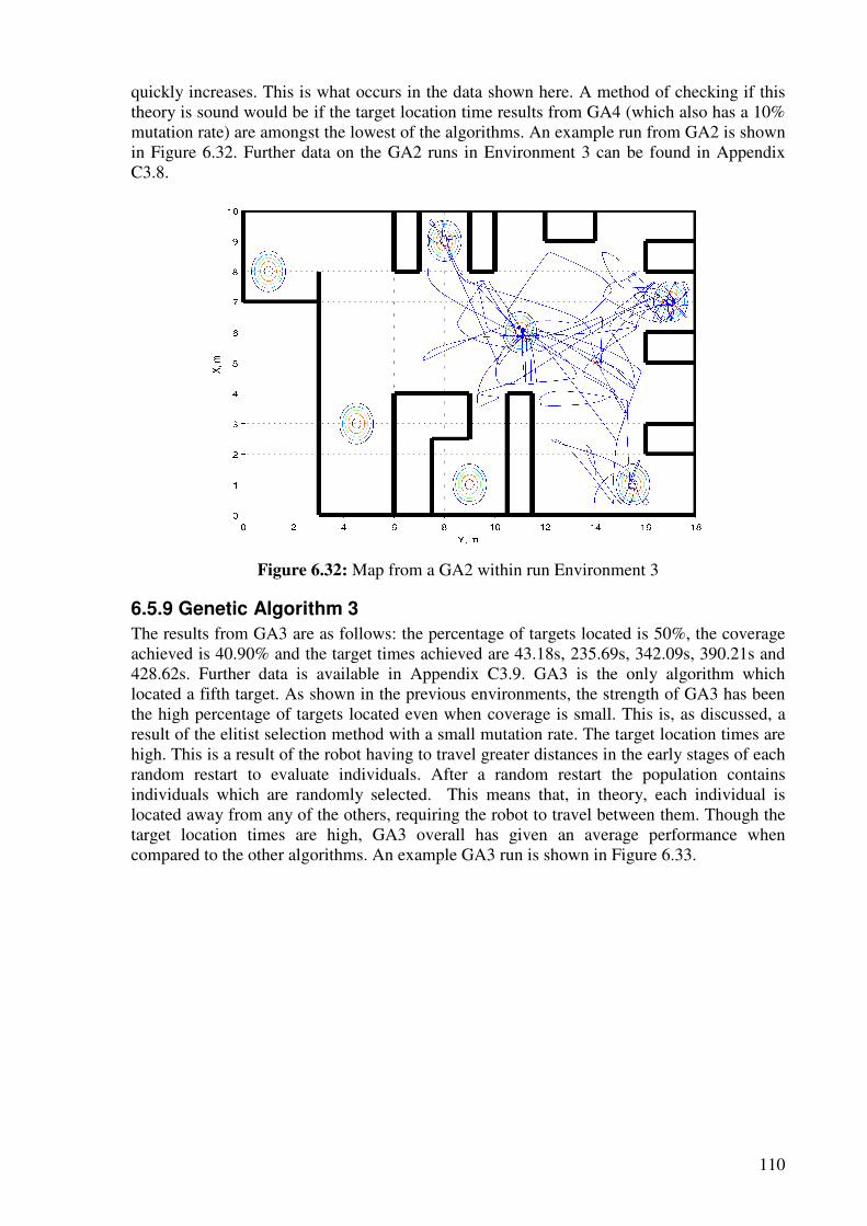
110
quickly increases. This is what occurs in the data shown here. A method of checking if this theory is sound would be if the target location time results from GA4 (which also has a 10% mutation rate) are amongst the lowest of the algorithms. An example run from GA2 is shown in Figure 6.32. Further data on the GA2 runs in Environment 3 can be found in Appendix C3.8.
Figure 6.32: Map from a GA2 within run Environment 3
6.5.9 Genetic Algorithm 3
The results from GA3 are as follows: the percentage of targets located is 50%, the coverage achieved is 40.90% and the target times achieved are 43.18s, 235.69s, 342.09s, 390.21s and 428.62s. Further data is available in Appendix C3.9. GA3 is the only algorithm which located a fifth target. As shown in the previous environments, the strength of GA3 has been the high percentage of targets located even when coverage is small. This is, as discussed, a result of the elitist selection method with a small mutation rate. The target location times are high. This is a result of the robot having to travel greater distances in the early stages of each random restart to evaluate individuals. After a random restart the population contains individuals which are randomly selected. This means that, in theory, each individual is located away from any of the others, requiring the robot to travel between them. Though the target location times are high, GA3 overall has given an average performance when compared to the other algorithms. An example GA3 run is shown in Figure 6.33.
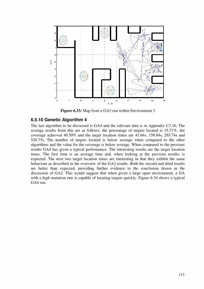
111
Figure 6.33: Map from a GA3 run within Environment 3
6.5.10 Genetic Algorithm 4
The last algorithm to be discussed is GA4 and the relevant data is in Appendix C3.10. The average results from this are as follows: the percentage of targets located is 35.71%, the coverage achieved 40.50% and the target location times are 41.64s, 158.84s, 265.74s and 526.75s. The number of targets located is below average when compared to the other algorithms and the value for the coverage is below average. When compared to the previous results GA4 has given a typical performance. The interesting results are the target location times. The first time is an average time and, when looking at the previous results, is expected. The next two target location times are interesting in that they exhibit the same behaviour as described in the overview of the GA2 results. Both the second and third results are better than expected, providing further evidence to the conclusion drawn in the discussion of GA2. This would suggest that when given a large open environment, a GA with a high mutation rate is capable of locating targets quickly. Figure 6.34 shows a typical GA4 run.
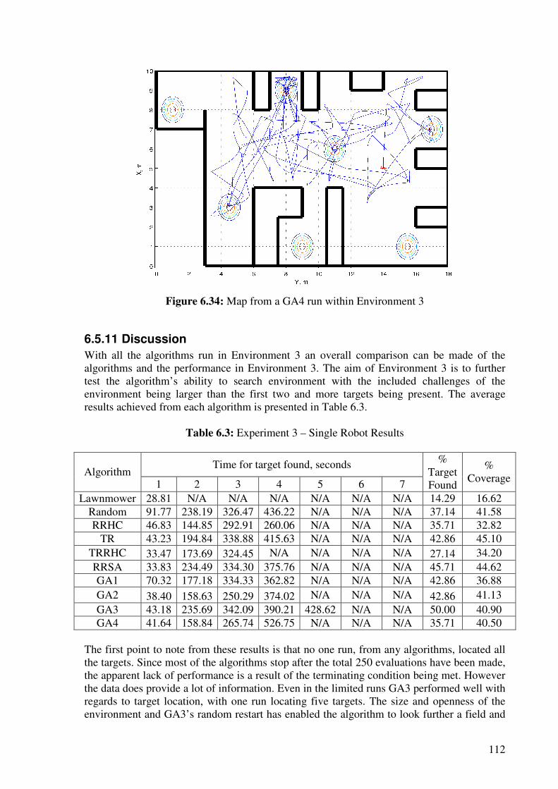
112
Figure 6.34: Map from a GA4 run within Environment 3
6.5.11 Discussion
With all the algorithms run in Environment 3 an overall comparison can be made of the algorithms and the performance in Environment 3. The aim of Environment 3 is to further test the algorithm’s ability to search environment with the included challenges of the environment being larger than the first two and more targets being present. The average results achieved from each algorithm is presented in Table 6.3.
Table 6.3: Experiment 3 – Single Robot Results
Time for target found, seconds Algorithm
1 2 3 4 5 6 7
% Target Found
% Coverage
Lawnmower 28.81 N/A N/A N/A N/A N/A N/A 14.29 16.62 Random 91.77 238.19 326.47 436.22 N/A N/A N/A 37.14 41.58 RRHC 46.83 144.85 292.91 260.06 N/A N/A N/A 35.71 32.82
TR 43.23 194.84 338.88 415.63 N/A N/A N/A 42.86 45.10 TRRHC 33.47 173.69 324.45 N/A N/A N/A N/A 27.14 34.20 RRSA 33.83 234.49 334.30 375.76 N/A N/A N/A 45.71 44.62 GA1 70.32 177.18 334.33 362.82 N/A N/A N/A 42.86 36.88 GA2 38.40 158.63 250.29 374.02 N/A N/A N/A 42.86 41.13 GA3 43.18 235.69 342.09 390.21 428.62 N/A N/A 50.00 40.90 GA4 41.64 158.84 265.74 526.75 N/A N/A N/A 35.71 40.50
The first point to note from these results is that no one run, from any algorithms, located all the targets. Since most of the algorithms stop after the total 250 evaluations have been made, the apparent lack of performance is a result of the terminating condition being met. However the data does provide a lot of information. Even in the limited runs GA3 performed well with regards to target location, with one run locating five targets. The size and openness of the environment and GA3’s random restart has enabled the algorithm to look further a field and
113
this has increased the chances of locating targets. Nevertheless the coverage is not as high as that achieved by other algorithms. This is the result of the dominance of a point which occurs when a target is almost located. The second point to note from the data presented is the difference between the time in the location of a first target and the location of a second target. In all the algorithms the difference is large. This indicates that when a dominant target exists, such as the target which is located beside the insertion point, the robot has a tendency to repeatedly migrate towards it. This dominant target has an effect on the algorithms running but the algorithms are still able to search the rest of the environment. Another point to note is the relationship between the coverage and the number of targets located. As the coverage increases, the number of targets located increases. It has been discussed that in order to achieve high coverage, an algorithm that contains a high random element within it should be used. Again the results show that there is a relationship between the random element in an algorithm, the coverage achieved by it and the number of targets located. Though the GAs do slightly work against this trend, they still fundamentally follow this relationship. The results also show, though not to as great an extent as found in the previous environments, that the algorithms which maintain a dominant point locate a first target quicker than other algorithms. However this seems to be the case only for the location of a first point, as the other target location times seem to vary, with the exception of the GA2 and GA4 times that both achieve quick times as discussed. Comparing the algorithms within Environment 3, the poorest performing is the Lawnmower. The reason for this is the inability of the algorithm to alter its path. The best performing algorithm, on average, is GA2. GA2 did not achieve the highest number of targets located or the highest coverage but the target location times it achieved have been consistently the highest, with the exception of the above average first target location time. The next algorithm to perform best is the RR Simulated Annealing, followed by GA3, GA4 and Tabu Random. GA3 is the average result of the group. Those algorithms that performed below average were the Random, GA1, Tabu RR HillClimbing and RR HillClimbing. From these results it can be seen that those algorithms that contain both a high random element and some structure to the selection of points perform well.
6.6 Summary
The objective of this chapter has been to establish if the algorithms presented in Chapter 5 can be used in the manner described in this work and to indicate, with regards to the results presented, which algorithm would be best suited to this use within a single robot case. It has been established that the algorithms discussed can be implemented in the task described, with the exception of the HillClimbing algorithm. This conclusion is backed up by the evidence provided throughout this chapter. With regards to the best performing algorithms in a single robot case, those algorithms that contain both a high random element and some structure to the selection of points perform well. The algorithms that show this are the Tabu
Random and RR Simulated Annealing algorithms and GA2, GA3 and GA4. Out of these five the best performing algorithm is hard to establish as there is not much of a performance difference between them. However the Tabu Random algorithm is simple to implement when compared to the other algorithms. Since it has similar results and is easier to implement, this algorithm would be the best choice for use in a single robot case.
114
The chapter started out by discussing the environments that each algorithm was to be tested in. The first environment that the algorithms have been tested in is discussed and what the aim of using this environment is, namely to test the algorithms to see if they can be used in this application. The second environment was designed with obstacles to enable the study of the impact obstacles have on the performance of the algorithms. Throughout all of the Environment 2 runs, and subsequently Environment 3, the method of obstacle avoidance implemented has been shown to work. The third environment has been designed to test if the algorithms could operate in larger environments. The results from the first environment were then presented. The majority of the algorithms showed that they can be used for this application. The exception is the HillClimbing algorithm which failed to make any impact. From the results presented it has been found that the algorithms which contained a high random element achieved better coverage, but the algorithms that allowed dominant points are able to locate the targets in a much quicker time. The chapter then presents the results from Environment 2. With the obstacles introduced the performance of the algorithms has been altered. However it is again seen that the algorithms which contained a high random element are able to achieve both a high coverage and locate a high number of targets. The final environment was then used to run the algorithms in. It has been shown that the algorithms do work in Environment 3 and that those algorithms which contained a high random element are able to achieve both a high coverage and locate a high number of targets. From the results presented in this chapter it can be seen that all the algorithms discussed in Chapter 5, with the exception of the basic HillClimbing algorithm, are suitable for the searching environments via a single robot. The results also show that algorithms which contain a high random element and have some control over how the next point is to be selected, namely Tabu Random and RR Simulated Annealing, provide good results. The results also show that Genetic Algorithms 2, 3 and 4, also provide good results. Though the other algorithms each have strengths the algorithms named consistently preformed well over all the environments and as such can be considered good candidates for the searching of environments when using a single robot. These algorithms may provide better results if adapted for use on a multi robot platform. The Tabu Random algorithm stood out throughout all the environments and as such would be a suitable algorithm for implementation.
115
Chapter 7
Simulation Results: Multi Robot
7.1 Introduction
The aim of the previous chapter was to establish if the algorithms presented in Chapter 5 can be used in the application described and which algorithms perform the best within a single robot case. It was established that the algorithms are suitable for use to achieve the aim of this work. However this was for a single robot case. The aim of this chapter is to establish if the best performing algorithms from the previous chapter can be used to control multiple robots and to consider if an improvement in the performance is achieved when employing such a multi robot approach. To achieve this aim the simulation used in this study has to be altered to be able to handle multiple robots and the interactions between them. After this stage the algorithms chosen to be run in the multi robot case will need to be selected and how the algorithms are to be implemented needs to be decided. The algorithms chosen are based on the results and conclusions from Chapter 6. To achieve the aim of this chapter the results will be studied and discussed. The first stage is to present the results, from each algorithm chosen, in the same manner as carried out in Chapter 6. From the results presented a discussion about how each algorithm has performed and how each algorithm performed with respect to the other algorithms run is presented. Since the ultimate aim of this chapter is to establish if the results presented here indicate a better performance in the task than those presented in Chapter 6, the results gained from the experiments carried out with regards to this chapter need to be compared to the results from the previous chapter. This comparison happens after the completion of the last algorithms in each environment. This chapter is structured as follows. Section 7.2 discusses the implementation of the multi robot simulation and which algorithms are to be used in this chapter. The results from the first environment are presented and discussed in Section 7.3, with a comparison made to the results in Chapter 6. Section 7.4 presents and discusses the results from runs carried out in Environment 2, again with comparisons made to the Environment 2 results from Chapter 6. The next section, Section 7.5, is concerned with the results gained from Environment 3. The penultimate section, Section 7.6, provides a review of all the results from both Chapters 6 and 7 and Section 7.7 presents a summary of this chapter.
7.2 Implementation
A simulation which can handle multiple robots needs to be implemented. Also the search algorithms to be run in the multi robot case need to be selected and suitably adapted to allow operation in the multi robot case. The environments and how the robots interact with one another also require consideration.
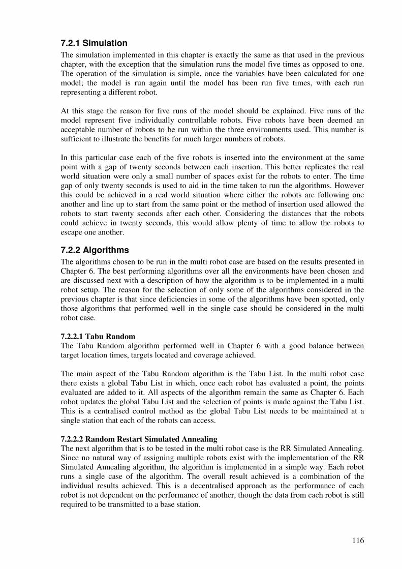
116
7.2.1 Simulation
The simulation implemented in this chapter is exactly the same as that used in the previous chapter, with the exception that the simulation runs the model five times as opposed to one. The operation of the simulation is simple, once the variables have been calculated for one model; the model is run again until the model has been run five times, with each run representing a different robot.
At this stage the reason for five runs of the model should be explained. Five runs of the model represent five individually controllable robots. Five robots have been deemed an acceptable number of robots to be run within the three environments used. This number is sufficient to illustrate the benefits for much larger numbers of robots. In this particular case each of the five robots is inserted into the environment at the same point with a gap of twenty seconds between each insertion. This better replicates the real world situation were only a small number of spaces exist for the robots to enter. The time gap of only twenty seconds is used to aid in the time taken to run the algorithms. However this could be achieved in a real world situation where either the robots are following one another and line up to start from the same point or the method of insertion used allowed the robots to start twenty seconds after each other. Considering the distances that the robots could achieve in twenty seconds, this would allow plenty of time to allow the robots to escape one another.
7.2.2 Algorithms
The algorithms chosen to be run in the multi robot case are based on the results presented in Chapter 6. The best performing algorithms over all the environments have been chosen and are discussed next with a description of how the algorithm is to be implemented in a multi robot setup. The reason for the selection of only some of the algorithms considered in the previous chapter is that since deficiencies in some of the algorithms have been spotted, only those algorithms that performed well in the single case should be considered in the multi robot case. 7.2.2.1 Tabu Random
The Tabu Random algorithm performed well in Chapter 6 with a good balance between target location times, targets located and coverage achieved. The main aspect of the Tabu Random algorithm is the Tabu List. In the multi robot case there exists a global Tabu List in which, once each robot has evaluated a point, the points evaluated are added to it. All aspects of the algorithm remain the same as Chapter 6. Each robot updates the global Tabu List and the selection of points is made against the Tabu List. This is a centralised control method as the global Tabu List needs to be maintained at a single station that each of the robots can access.
7.2.2.2 Random Restart Simulated Annealing
The next algorithm that is to be tested in the multi robot case is the RR Simulated Annealing. Since no natural way of assigning multiple robots exist with the implementation of the RR Simulated Annealing algorithm, the algorithm is implemented in a simple way. Each robot runs a single case of the algorithm. The overall result achieved is a combination of the individual results achieved. This is a decentralised approach as the performance of each robot is not dependent on the performance of another, though the data from each robot is still required to be transmitted to a base station.
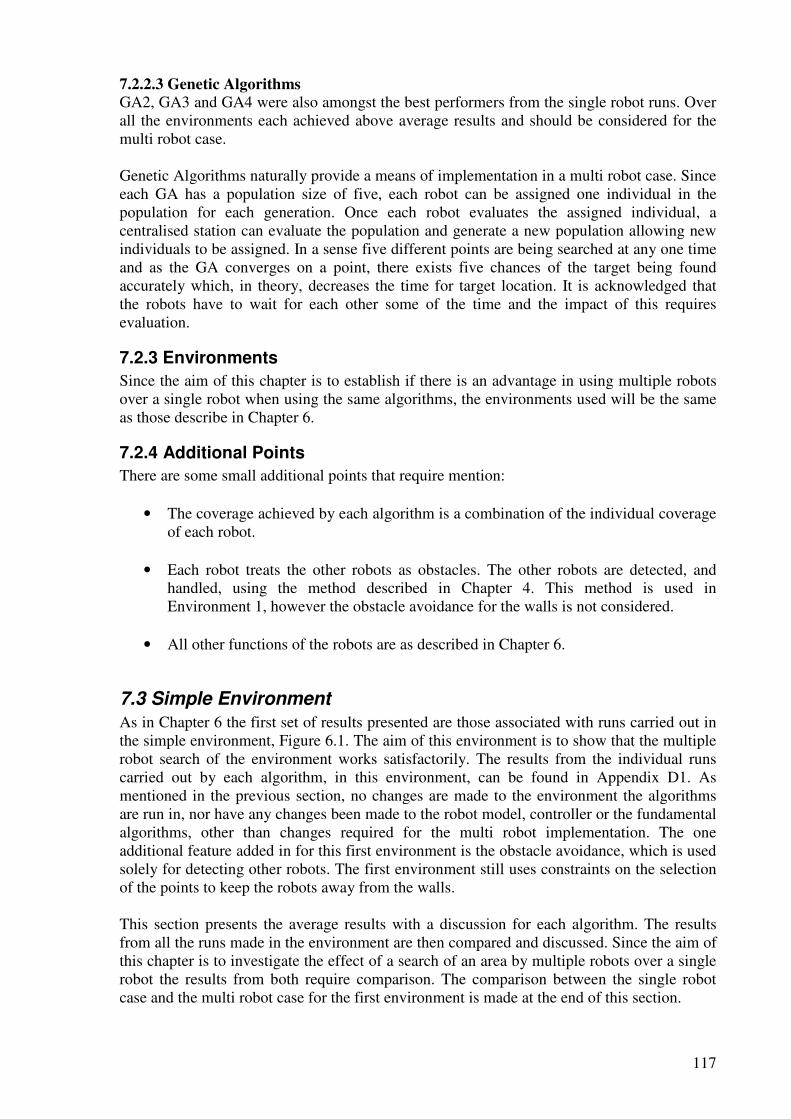
117
7.2.2.3 Genetic Algorithms
GA2, GA3 and GA4 were also amongst the best performers from the single robot runs. Over all the environments each achieved above average results and should be considered for the multi robot case. Genetic Algorithms naturally provide a means of implementation in a multi robot case. Since each GA has a population size of five, each robot can be assigned one individual in the population for each generation. Once each robot evaluates the assigned individual, a centralised station can evaluate the population and generate a new population allowing new individuals to be assigned. In a sense five different points are being searched at any one time and as the GA converges on a point, there exists five chances of the target being found accurately which, in theory, decreases the time for target location. It is acknowledged that the robots have to wait for each other some of the time and the impact of this requires evaluation.
7.2.3 Environments
Since the aim of this chapter is to establish if there is an advantage in using multiple robots over a single robot when using the same algorithms, the environments used will be the same as those describe in Chapter 6.
7.2.4 Additional Points
There are some small additional points that require mention:
• The coverage achieved by each algorithm is a combination of the individual coverage of each robot.
• Each robot treats the other robots as obstacles. The other robots are detected, and
handled, using the method described in Chapter 4. This method is used in Environment 1, however the obstacle avoidance for the walls is not considered.
• All other functions of the robots are as described in Chapter 6.
7.3 Simple Environment
As in Chapter 6 the first set of results presented are those associated with runs carried out in the simple environment, Figure 6.1. The aim of this environment is to show that the multiple robot search of the environment works satisfactorily. The results from the individual runs carried out by each algorithm, in this environment, can be found in Appendix D1. As mentioned in the previous section, no changes are made to the environment the algorithms are run in, nor have any changes been made to the robot model, controller or the fundamental algorithms, other than changes required for the multi robot implementation. The one additional feature added in for this first environment is the obstacle avoidance, which is used solely for detecting other robots. The first environment still uses constraints on the selection of the points to keep the robots away from the walls. This section presents the average results with a discussion for each algorithm. The results from all the runs made in the environment are then compared and discussed. Since the aim of this chapter is to investigate the effect of a search of an area by multiple robots over a single robot the results from both require comparison. The comparison between the single robot case and the multi robot case for the first environment is made at the end of this section.
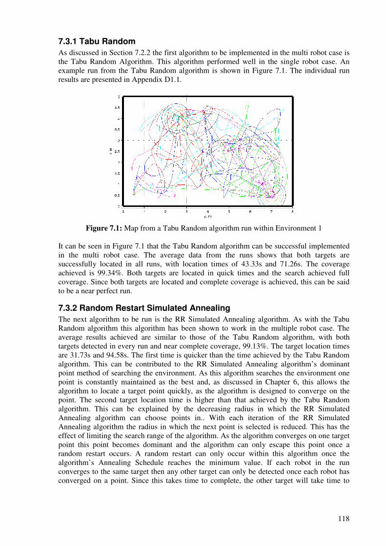
118
7.3.1 Tabu Random
As discussed in Section 7.2.2 the first algorithm to be implemented in the multi robot case is the Tabu Random Algorithm. This algorithm performed well in the single robot case. An example run from the Tabu Random algorithm is shown in Figure 7.1. The individual run results are presented in Appendix D1.1.
Figure 7.1: Map from a Tabu Random algorithm run within Environment 1
It can be seen in Figure 7.1 that the Tabu Random algorithm can be successful implemented in the multi robot case. The average data from the runs shows that both targets are successfully located in all runs, with location times of 43.33s and 71.26s. The coverage achieved is 99.34%. Both targets are located in quick times and the search achieved full coverage. Since both targets are located and complete coverage is achieved, this can be said to be a near perfect run.
7.3.2 Random Restart Simulated Annealing
The next algorithm to be run is the RR Simulated Annealing algorithm. As with the Tabu Random algorithm this algorithm has been shown to work in the multiple robot case. The average results achieved are similar to those of the Tabu Random algorithm, with both targets detected in every run and near complete coverage, 99.13%. The target location times are 31.73s and 94.58s. The first time is quicker than the time achieved by the Tabu Random algorithm. This can be contributed to the RR Simulated Annealing algorithm’s dominant point method of searching the environment. As this algorithm searches the environment one point is constantly maintained as the best and, as discussed in Chapter 6, this allows the algorithm to locate a target point quickly, as the algorithm is designed to converge on the point. The second target location time is higher than that achieved by the Tabu Random algorithm. This can be explained by the decreasing radius in which the RR Simulated Annealing algorithm can choose points in.. With each iteration of the RR Simulated Annealing algorithm the radius in which the next point is selected is reduced. This has the effect of limiting the search range of the algorithm. As the algorithm converges on one target point this point becomes dominant and the algorithm can only escape this point once a random restart occurs. A random restart can only occur within this algorithm once the algorithm’s Annealing Schedule reaches the minimum value. If each robot in the run converges to the same target then any other target can only be detected once each robot has converged on a point. Since this takes time to complete, the other target will take time to
119
locate. Figure 7.2 shows an example run from the RR Simulated Annealing algorithm. Appendix D1.2 contains the individual run data for the Simulated Annealing algorithm.
Figure 7.2: Map from RR Simulated Annealing algorithm run within Environment 1
7.3.3 Genetic Algorithm 2
The first of the Genetic Algorithms to be run is GA2. As with the first two algorithms presented, GA2 has shown to work in the multiple robot case. The average results gained from GA2 are as follows: both targets were located in every run with an average of 97.92% coverage. The target location times are 41.27s and 155.31s. Although GA2 did achieve near full coverage, the coverage achieved is lower than that of both the Tabu Random and RR Simulated Annealing algorithms. The reason for this slightly reduced coverage is that the algorithm is attracted to either one of the targets and remains in the vicinity of the targets or is at a point travelling between the targets. While doing this the algorithm is leaving a small area at the bottom of the environment unsearched. This has occurred in each run and shows the algorithm’s reliance on having a target within the environment. The first target time is not as quick as that achieved by the RR Simulated Annealing. However it is slightly quicker than that achieved by the Tabu Random algorithm. This shows that GA2 can quickly converge on a point as previously discussed. On the other hand, the second target location time is the poorest time yet. One reason for this is the interaction between the robots within the algorithm. As the robots converge on a target point, the interaction between them increases. Since the robots treat one another as obstacles, the robots stop and reassign the points they are to evaluate. This continues to happen until no obstacles are present within the range of the robot’s sensor. Since the robots are crowded into one area it takes time for each robot to escape the sensor range of the other robots. Hence the search slows while the robots try to travel away from each other. This slows the search as technically no robot is searching the environment and when one robot does move away from the other robots, once it reaches the point it is to evaluate, it remains there until the other robots have evaluated the points assigned to them. This process takes time and as a result the location time, once one target has been located, will be high. An example run from GA2 is shown in Figure 7.3 with the individual run data presented in Appendix D1.3.
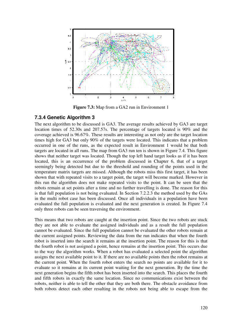
120
Figure 7.3: Map from a GA2 run in Environment 1
7.3.4 Genetic Algorithm 3
The next algorithm to be discussed is GA3. The average results achieved by GA3 are target location times of 52.30s and 207.57s. The percentage of targets located is 90% and the coverage achieved is 96.67%. These results are interesting as not only are the target location times high for GA3 but only 90% of the targets were located. This indicates that a problem occurred in one of the runs, as the expected result in Environment 1 would be that both targets are located in all runs. The map from GA3 run ten is shown in Figure 7.4. This figure shows that neither target was located. Though the top left hand target looks as if it has been located, this is an occurrence of the problem discussed in Chapter 6, that of a target seemingly being detected but due to the threshold and rounding of the points used in the temperature matrix targets are missed. Although the robots miss this first target, it has been shown that with repeated visits to a target point, the target will become marked. However in this run the algorithm does not make repeated visits to the point. It can be seen that the robots remain at set points after a time and no further travelling is done. The reason for this is that full population is not being evaluated. In Section 7.2.2.3 the method used by the GAs in the multi robot case has been discussed. Once all individuals in a population have been evaluated the full population is evaluated and the next generation is created. In Figure 7.4 only three robots can be seen traversing the environment. This means that two robots are caught at the insertion point. Since the two robots are stuck they are not able to evaluate the assigned individuals and as a result the full population cannot be evaluated. Since the full population cannot be evaluated the other robots remain at the current assigned points. Reviewing the data from the run indicates that when the fourth robot is inserted into the search it remains at the insertion point. The reason for this is that the fourth robot is not assigned a point, hence remains at the insertion point. This occurs due to the way the algorithm works. When a robot has evaluated a selected point the algorithm assigns the next available point to it. If there are no available points then the robot remains at the current point. When the fourth robot enters the search no points are available for it to evaluate so it remains at its current point waiting for the next generation. By the time the next generation begins the fifth robot has been inserted into the search. This places the fourth and fifth robots in exactly the same location. Since no communications exist between the robots, neither is able to tell the other that they are both there. The obstacle avoidance from both robots detect each other resulting in the robots not being able to escape from the
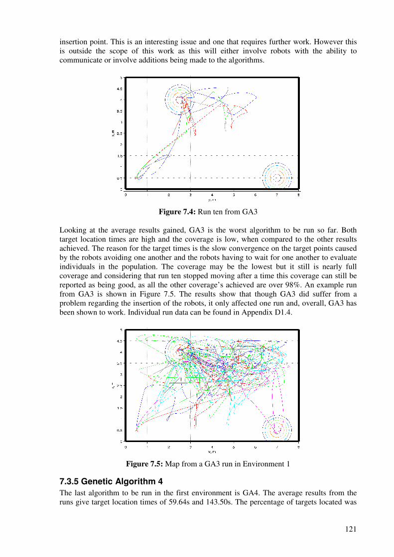
121
insertion point. This is an interesting issue and one that requires further work. However this is outside the scope of this work as this will either involve robots with the ability to communicate or involve additions being made to the algorithms.
Figure 7.4: Run ten from GA3
Looking at the average results gained, GA3 is the worst algorithm to be run so far. Both target location times are high and the coverage is low, when compared to the other results achieved. The reason for the target times is the slow convergence on the target points caused by the robots avoiding one another and the robots having to wait for one another to evaluate individuals in the population. The coverage may be the lowest but it still is nearly full coverage and considering that run ten stopped moving after a time this coverage can still be reported as being good, as all the other coverage’s achieved are over 98%. An example run from GA3 is shown in Figure 7.5. The results show that though GA3 did suffer from a problem regarding the insertion of the robots, it only affected one run and, overall, GA3 has been shown to work. Individual run data can be found in Appendix D1.4.
Figure 7.5: Map from a GA3 run in Environment 1
7.3.5 Genetic Algorithm 4
The last algorithm to be run in the first environment is GA4. The average results from the runs give target location times of 59.64s and 143.50s. The percentage of targets located was
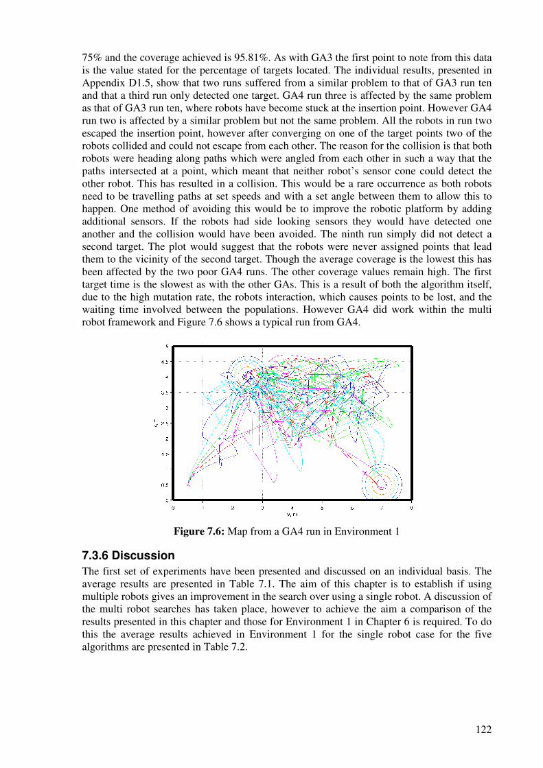
122
75% and the coverage achieved is 95.81%. As with GA3 the first point to note from this data is the value stated for the percentage of targets located. The individual results, presented in Appendix D1.5, show that two runs suffered from a similar problem to that of GA3 run ten and that a third run only detected one target. GA4 run three is affected by the same problem as that of GA3 run ten, where robots have become stuck at the insertion point. However GA4 run two is affected by a similar problem but not the same problem. All the robots in run two escaped the insertion point, however after converging on one of the target points two of the robots collided and could not escape from each other. The reason for the collision is that both robots were heading along paths which were angled from each other in such a way that the paths intersected at a point, which meant that neither robot’s sensor cone could detect the other robot. This has resulted in a collision. This would be a rare occurrence as both robots need to be travelling paths at set speeds and with a set angle between them to allow this to happen. One method of avoiding this would be to improve the robotic platform by adding additional sensors. If the robots had side looking sensors they would have detected one another and the collision would have been avoided. The ninth run simply did not detect a second target. The plot would suggest that the robots were never assigned points that lead them to the vicinity of the second target. Though the average coverage is the lowest this has been affected by the two poor GA4 runs. The other coverage values remain high. The first target time is the slowest as with the other GAs. This is a result of both the algorithm itself, due to the high mutation rate, the robots interaction, which causes points to be lost, and the waiting time involved between the populations. However GA4 did work within the multi robot framework and Figure 7.6 shows a typical run from GA4.
Figure 7.6: Map from a GA4 run in Environment 1
7.3.6 Discussion
The first set of experiments have been presented and discussed on an individual basis. The average results are presented in Table 7.1. The aim of this chapter is to establish if using multiple robots gives an improvement in the search over using a single robot. A discussion of the multi robot searches has taken place, however to achieve the aim a comparison of the results presented in this chapter and those for Environment 1 in Chapter 6 is required. To do this the average results achieved in Environment 1 for the single robot case for the five algorithms are presented in Table 7.2.
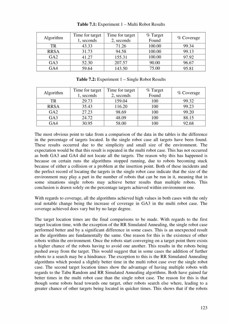
123
Table 7.1: Experiment 1 – Multi Robot Results
Algorithm Time for target
1, seconds Time for target
2, seconds % Target
Found % Coverage
TR 43.33 71.26 100.00 99.34 RRSA 31.73 94.58 100.00 99.13 GA2 41.27 155.31 100.00 97.92 GA3 52.30 207.57 90.00 96.67 GA4 59.64 143.50 75.00 95.81
Table 7.2: Experiment 1 – Single Robot Results
Algorithm Time for target
1, seconds Time for target
2, seconds % Target
Found % Coverage
TR 29.73 159.04 100 99.32 RRSA 35.43 116.20 100 99.23 GA2 27.23 98.69 100 99.20 GA3 24.72 48.09 100 88.15 GA4 30.95 58.00 100 92.68
The most obvious point to take from a comparison of the data in the tables is the difference in the percentage of targets located. In the single robot case all targets have been found. These results occurred due to the simplicity and small size of the environment. The expectation would be that this result is repeated in the multi robot case. This has not occurred as both GA3 and GA4 did not locate all the targets. The reason why this has happened is because on certain runs the algorithms stopped running, due to robots becoming stuck because of either a collision or a problem at the insertion point. Both of these incidents and the perfect record of locating the targets in the single robot case indicate that the size of the environment may play a part in the number of robots that can be run in it, meaning that in some situations single robots may achieve better results than multiple robots. This conclusion is drawn solely on the percentage targets achieved within environment one. With regards to coverage, all the algorithms achieved high values in both cases with the only real notable change being the increase of coverage in GA3 in the multi robot case. The coverage achieved does vary but by no large degree. The target location times are the final comparisons to be made. With regards to the first target location time, with the exception of the RR Simulated Annealing, the single robot case performed better and by a significant difference in some cases. This is an unexpected result as the algorithms are fundamentally the same. One reason for this is the existence of other robots within the environment. Once the robots start converging on a target point there exists a higher chance of the robots having to avoid one another. This results in the robots being pushed away from the target. This would suggest that in some cases the addition of further robots to a search may be a hindrance. The exception to this is the RR Simulated Annealing algorithms which posted a slightly better time in the multi robot case over the single robot case. The second target location times show the advantage of having multiple robots with regards to the Tabu Random and RR Simulated Annealing algorithms. Both have gained far better times in the multi robot case than the single robot case. The reason for this is that though some robots head towards one target, other robots search else where, leading to a greater chance of other targets being located in quicker times. This shows that if the robots
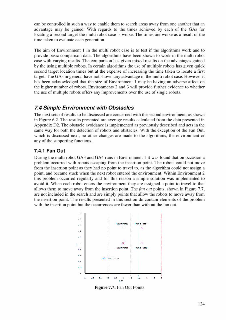
124
can be controlled in such a way to enable them to search areas away from one another that an advantage may be gained. With regards to the times achieved by each of the GAs for locating a second target the multi robot case is worse. The times are worse as a result of the time taken to evaluate each generation. The aim of Environment 1 in the multi robot case is to test if the algorithms work and to provide basic comparison data. The algorithms have been shown to work in the multi robot case with varying results. The comparison has given mixed results on the advantages gained by the using multiple robots. In certain algorithms the use of multiple robots has given quick second target location times but at the expense of increasing the time taken to locate a first target. The GAs in general have not shown any advantage in the multi robot case. However it has been acknowledged that the size of Environment 1 may be having an adverse affect on the higher number of robots. Environments 2 and 3 will provide further evidence to whether the use of multiple robots offers any improvements over the use of single robots.
7.4 Simple Environment with Obstacles
The next sets of results to be discussed are concerned with the second environment, as shown in Figure 6.2. The results presented are average results calculated from the data presented in Appendix D2. The obstacle avoidance is implemented as previously described and acts in the same way for both the detection of robots and obstacles. With the exception of the Fan Out, which is discussed next, no other changes are made to the algorithms, the environment or any of the supporting functions.
7.4.1 Fan Out
During the multi robot GA3 and GA4 runs in Environment 1 it was found that on occasion a problem occurred with robots escaping from the insertion point. The robots could not move from the insertion point as they had no point to travel to, as the algorithm could not assign a point, and became stuck when the next robot entered the environment. Within Environment 2 this problem occurred regularly and for this reason a simple solution was implemented to avoid it. When each robot enters the environment they are assigned a point to travel to that allows them to move away from the insertion point. The fan out points, shown in Figure 7.7, are not included in the search and are simply points that allow the robots to move away from the insertion point. The results presented in this section do contain elements of the problem with the insertion point but the occurrences are fewer than without the fan out.
Figure 7.7: Fan Out Points
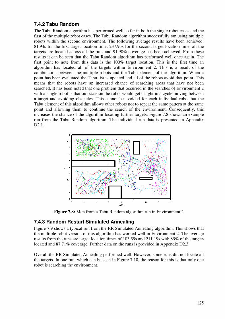
125
7.4.2 Tabu Random
The Tabu Random algorithm has performed well so far in both the single robot cases and the first of the multiple robot cases. The Tabu Random algorithm successfully ran using multiple robots within the second environment. The following average results have been achieved: 81.94s for the first target location time, 237.95s for the second target location time, all the targets are located across all the runs and 91.90% coverage has been achieved. From these results it can be seen that the Tabu Random algorithm has performed well once again. The first point to note from this data is the 100% target location. This is the first time an algorithm has located all of the targets within Environment 2. This is a result of the combination between the multiple robots and the Tabu element of the algorithm. When a point has been evaluated the Tabu list is updated and all of the robots avoid that point. This means that the robots have an increased chance of searching areas that have not been searched. It has been noted that one problem that occurred in the searches of Environment 2 with a single robot is that on occasion the robot would get caught in a cycle moving between a target and avoiding obstacles. This cannot be avoided for each individual robot but the Tabu element of this algorithm allows other robots not to repeat the same pattern at the same point and allowing them to continue the search of the environment. Consequently, this increases the chance of the algorithm locating further targets. Figure 7.8 shows an example run from the Tabu Random algorithm. The individual run data is presented in Appendix D2.1.
Figure 7.8: Map from a Tabu Random algorithm run in Environment 2
7.4.3 Random Restart Simulated Annealing
Figure 7.9 shows a typical run from the RR Simulated Annealing algorithm. This shows that the multiple robot version of this algorithm has worked well in Environment 2. The average results from the runs are target location times of 103.59s and 211.19s with 85% of the targets located and 87.71% coverage. Further data on the runs is provided in Appendix D2.3. Overall the RR Simulated Annealing performed well. However, some runs did not locate all the targets. In one run, which can be seen in Figure 7.10, the reason for this is that only one robot is searching the environment.
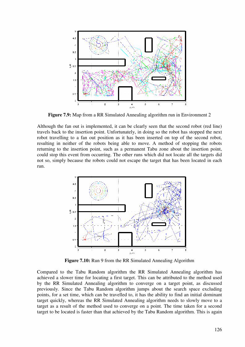
126
Figure 7.9: Map from a RR Simulated Annealing algorithm run in Environment 2
Although the fan out is implemented, it can be clearly seen that the second robot (red line) travels back to the insertion point. Unfortunately, in doing so the robot has stopped the next robot travelling to a fan out position as it has been inserted on top of the second robot, resulting in neither of the robots being able to move. A method of stopping the robots returning to the insertion point, such as a permanent Tabu zone about the insertion point, could stop this event from occurring. The other runs which did not locate all the targets did not so, simply because the robots could not escape the target that has been located in each run.
Figure 7.10: Run 9 from the RR Simulated Annealing Algorithm
Compared to the Tabu Random algorithm the RR Simulated Annealing algorithm has achieved a slower time for locating a first target. This can be attributed to the method used by the RR Simulated Annealing algorithm to converge on a target point, as discussed previously. Since the Tabu Random algorithm jumps about the search space excluding points, for a set time, which can be travelled to, it has the ability to find an initial dominant target quickly, whereas the RR Simulated Annealing algorithm needs to slowly move to a target as a result of the method used to converge on a point. The time taken for a second target to be located is faster than that achieved by the Tabu Random algorithm. This is again
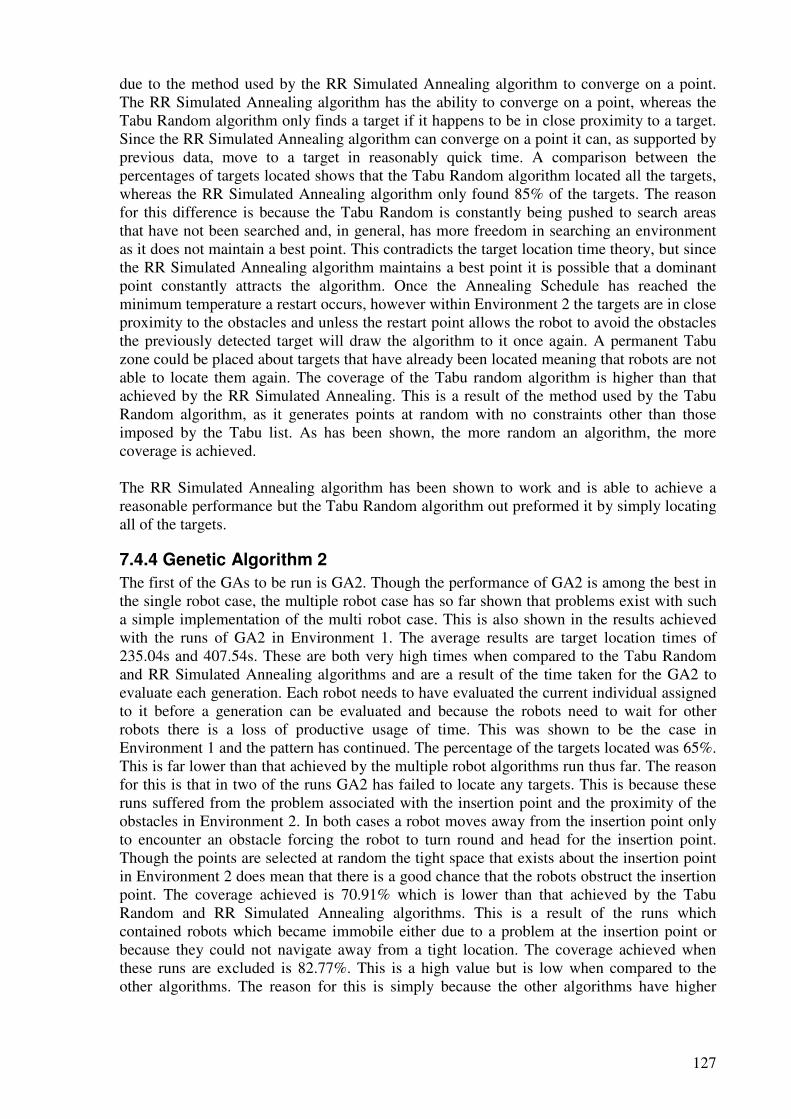
127
due to the method used by the RR Simulated Annealing algorithm to converge on a point. The RR Simulated Annealing algorithm has the ability to converge on a point, whereas the Tabu Random algorithm only finds a target if it happens to be in close proximity to a target. Since the RR Simulated Annealing algorithm can converge on a point it can, as supported by previous data, move to a target in reasonably quick time. A comparison between the percentages of targets located shows that the Tabu Random algorithm located all the targets, whereas the RR Simulated Annealing algorithm only found 85% of the targets. The reason for this difference is because the Tabu Random is constantly being pushed to search areas that have not been searched and, in general, has more freedom in searching an environment as it does not maintain a best point. This contradicts the target location time theory, but since the RR Simulated Annealing algorithm maintains a best point it is possible that a dominant point constantly attracts the algorithm. Once the Annealing Schedule has reached the minimum temperature a restart occurs, however within Environment 2 the targets are in close proximity to the obstacles and unless the restart point allows the robot to avoid the obstacles the previously detected target will draw the algorithm to it once again. A permanent Tabu zone could be placed about targets that have already been located meaning that robots are not able to locate them again. The coverage of the Tabu random algorithm is higher than that achieved by the RR Simulated Annealing. This is a result of the method used by the Tabu Random algorithm, as it generates points at random with no constraints other than those imposed by the Tabu list. As has been shown, the more random an algorithm, the more coverage is achieved. The RR Simulated Annealing algorithm has been shown to work and is able to achieve a reasonable performance but the Tabu Random algorithm out preformed it by simply locating all of the targets.
7.4.4 Genetic Algorithm 2
The first of the GAs to be run is GA2. Though the performance of GA2 is among the best in the single robot case, the multiple robot case has so far shown that problems exist with such a simple implementation of the multi robot case. This is also shown in the results achieved with the runs of GA2 in Environment 1. The average results are target location times of 235.04s and 407.54s. These are both very high times when compared to the Tabu Random and RR Simulated Annealing algorithms and are a result of the time taken for the GA2 to evaluate each generation. Each robot needs to have evaluated the current individual assigned to it before a generation can be evaluated and because the robots need to wait for other robots there is a loss of productive usage of time. This was shown to be the case in Environment 1 and the pattern has continued. The percentage of the targets located was 65%. This is far lower than that achieved by the multiple robot algorithms run thus far. The reason for this is that in two of the runs GA2 has failed to locate any targets. This is because these runs suffered from the problem associated with the insertion point and the proximity of the obstacles in Environment 2. In both cases a robot moves away from the insertion point only to encounter an obstacle forcing the robot to turn round and head for the insertion point. Though the points are selected at random the tight space that exists about the insertion point in Environment 2 does mean that there is a good chance that the robots obstruct the insertion point. The coverage achieved is 70.91% which is lower than that achieved by the Tabu Random and RR Simulated Annealing algorithms. This is a result of the runs which contained robots which became immobile either due to a problem at the insertion point or because they could not navigate away from a tight location. The coverage achieved when these runs are excluded is 82.77%. This is a high value but is low when compared to the other algorithms. The reason for this is simply because the other algorithms have higher
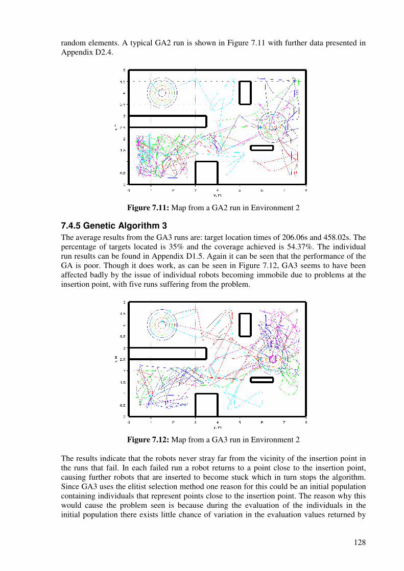
128
random elements. A typical GA2 run is shown in Figure 7.11 with further data presented in Appendix D2.4.
Figure 7.11: Map from a GA2 run in Environment 2
7.4.5 Genetic Algorithm 3
The average results from the GA3 runs are: target location times of 206.06s and 458.02s. The percentage of targets located is 35% and the coverage achieved is 54.37%. The individual run results can be found in Appendix D1.5. Again it can be seen that the performance of the GA is poor. Though it does work, as can be seen in Figure 7.12, GA3 seems to have been affected badly by the issue of individual robots becoming immobile due to problems at the insertion point, with five runs suffering from the problem.
Figure 7.12: Map from a GA3 run in Environment 2
The results indicate that the robots never stray far from the vicinity of the insertion point in the runs that fail. In each failed run a robot returns to a point close to the insertion point, causing further robots that are inserted to become stuck which in turn stops the algorithm. Since GA3 uses the elitist selection method one reason for this could be an initial population containing individuals that represent points close to the insertion point. The reason why this would cause the problem seen is because during the evaluation of the individuals in the initial population there exists little chance of variation in the evaluation values returned by
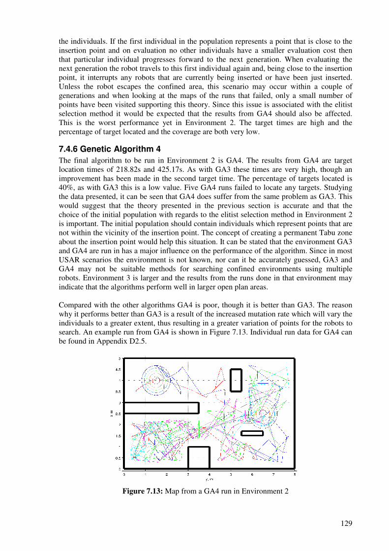
129
the individuals. If the first individual in the population represents a point that is close to the insertion point and on evaluation no other individuals have a smaller evaluation cost then that particular individual progresses forward to the next generation. When evaluating the next generation the robot travels to this first individual again and, being close to the insertion point, it interrupts any robots that are currently being inserted or have been just inserted. Unless the robot escapes the confined area, this scenario may occur within a couple of generations and when looking at the maps of the runs that failed, only a small number of points have been visited supporting this theory. Since this issue is associated with the elitist selection method it would be expected that the results from GA4 should also be affected. This is the worst performance yet in Environment 2. The target times are high and the percentage of target located and the coverage are both very low.
7.4.6 Genetic Algorithm 4
The final algorithm to be run in Environment 2 is GA4. The results from GA4 are target location times of 218.82s and 425.17s. As with GA3 these times are very high, though an improvement has been made in the second target time. The percentage of targets located is 40%, as with GA3 this is a low value. Five GA4 runs failed to locate any targets. Studying the data presented, it can be seen that GA4 does suffer from the same problem as GA3. This would suggest that the theory presented in the previous section is accurate and that the choice of the initial population with regards to the elitist selection method in Environment 2 is important. The initial population should contain individuals which represent points that are not within the vicinity of the insertion point. The concept of creating a permanent Tabu zone about the insertion point would help this situation. It can be stated that the environment GA3 and GA4 are run in has a major influence on the performance of the algorithm. Since in most USAR scenarios the environment is not known, nor can it be accurately guessed, GA3 and GA4 may not be suitable methods for searching confined environments using multiple robots. Environment 3 is larger and the results from the runs done in that environment may indicate that the algorithms perform well in larger open plan areas. Compared with the other algorithms GA4 is poor, though it is better than GA3. The reason why it performs better than GA3 is a result of the increased mutation rate which will vary the individuals to a greater extent, thus resulting in a greater variation of points for the robots to search. An example run from GA4 is shown in Figure 7.13. Individual run data for GA4 can be found in Appendix D2.5.
Figure 7.13: Map from a GA4 run in Environment 2
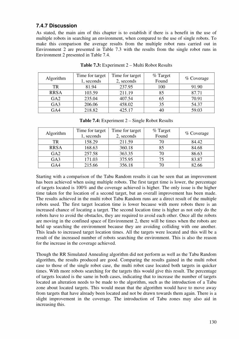
130
7.4.7 Discussion
As stated, the main aim of this chapter is to establish if there is a benefit in the use of multiple robots in searching an environment, when compared to the use of single robots. To make this comparison the average results from the multiple robot runs carried out in Environment 2 are presented in Table 7.3 with the results from the single robot runs in Environment 2 presented in Table 7.4.
Table 7.3: Experiment 2 – Multi Robot Results
Algorithm Time for target
1, seconds Time for target
2, seconds % Target
Found % Coverage
TR 81.94 237.95 100 91.90 RRSA 103.59 211.19 85 87.71 GA2 235.04 407.54 65 70.91 GA3 206.06 458.02 35 54.37 GA4 218.82 425.17 40 59.03
Table 7.4: Experiment 2 – Single Robot Results
Algorithm Time for target
1, seconds Time for target
2, seconds % Target
Found % Coverage
TR 158.29 211.59 70 84.42 RRSA 168.63 360.18 85 84.68 GA2 257.58 363.35 70 86.63 GA3 171.03 375.95 75 83.87 GA4 215.66 356.18 70 82.66
Starting with a comparison of the Tabu Random results it can be seen that an improvement has been achieved when using multiple robots. The first target time is lower, the percentage of targets located is 100% and the coverage achieved is higher. The only issue is the higher time taken for the location of a second target, but an overall improvement has been made. The results achieved in the multi robot Tabu Random runs are a direct result of the multiple robots used. The first target location time is lower because with more robots there is an increased chance of locating a target. The second location time is higher as not only do the robots have to avoid the obstacles, they are required to avoid each other. Once all the robots are moving in the confined space of Environment 2, there will be times when the robots are held up searching the environment because they are avoiding colliding with one another. This leads to increased target location times. All the targets were located and this will be a result of the increased number of robots searching the environment. This is also the reason for the increase in the coverage achieved. Though the RR Simulated Annealing algorithm did not perform as well as the Tabu Random algorithm, the results produced are good. Comparing the results gained in the multi robot case to those of the single robot case, the multi robot case located both targets in quicker times. With more robots searching for the targets this would give this result. The percentage of targets located is the same in both cases, indicating that to increase the number of targets located an alteration needs to be made to the algorithm, such as the introduction of a Tabu zone about located targets. This would mean that the algorithm would have to move away from targets that have already been located and not be drawn towards them again. There is a slight improvement in the coverage. The introduction of Tabu zones may also aid in increasing this.
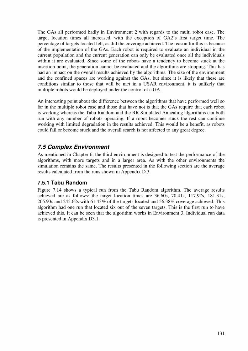
131
The GAs all performed badly in Environment 2 with regards to the multi robot case. The target location times all increased, with the exception of GA2’s first target time. The percentage of targets located fell, as did the coverage achieved. The reason for this is because of the implementation of the GAs. Each robot is required to evaluate an individual in the current population and the current generation can only be evaluated once all the individuals within it are evaluated. Since some of the robots have a tendency to become stuck at the insertion point, the generation cannot be evaluated and the algorithms are stopping. This has had an impact on the overall results achieved by the algorithms. The size of the environment and the confined spaces are working against the GAs, but since it is likely that these are conditions similar to those that will be met in a USAR environment, it is unlikely that multiple robots would be deployed under the control of a GA. An interesting point about the difference between the algorithms that have performed well so far in the multiple robot case and those that have not is that the GAs require that each robot is working whereas the Tabu Random and the RR Simulated Annealing algorithms can both run with any number of robots operating. If a robot becomes stuck the rest can continue working with limited degradation in the results achieved. This would be a benefit, as robots could fail or become stuck and the overall search is not affected to any great degree.
7.5 Complex Environment
As mentioned in Chapter 6, the third environment is designed to test the performance of the algorithms, with more targets and in a larger area. As with the other environments the simulation remains the same. The results presented in the following section are the average results calculated from the runs shown in Appendix D.3.
7.5.1 Tabu Random
Figure 7.14 shows a typical run from the Tabu Random algorithm. The average results achieved are as follows: the target location times are 36.60s, 70.41s, 117.97s, 181.31s, 205.93s and 245.62s with 61.43% of the targets located and 56.38% coverage achieved. This algorithm had one run that located six out of the seven targets. This is the first run to have achieved this. It can be seen that the algorithm works in Environment 3. Individual run data is presented in Appendix D3.1.
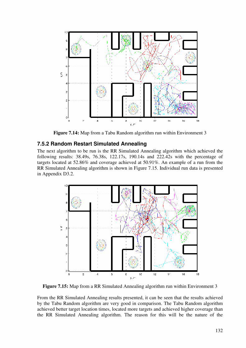
132
Figure 7.14: Map from a Tabu Random algorithm run within Environment 3
7.5.2 Random Restart Simulated Annealing
The next algorithm to be run is the RR Simulated Annealing algorithm which achieved the following results: 38.49s, 76.38s, 122.17s, 190.14s and 222.42s with the percentage of targets located at 52.86% and coverage achieved at 50.91%. An example of a run from the RR Simulated Annealing algorithm is shown in Figure 7.15. Individual run data is presented in Appendix D3.2.
Figure 7.15: Map from a RR Simulated Annealing algorithm run within Environment 3
From the RR Simulated Annealing results presented, it can be seen that the results achieved by the Tabu Random algorithm are very good in comparison. The Tabu Random algorithm achieved better target location times, located more targets and achieved higher coverage than the RR Simulated Annealing algorithm. The reason for this will be the nature of the
133
environment and the method used by each algorithm to search the environment. Since this environment is more open there is less interaction with obstacles, which allows the algorithms to search the environment with minimal interruption. Since the Tabu Random algorithm can select points at random, with the exception of those points on the Tabu list, wider open spaces allow the robots to move without hindrance to the assigned points. This free movement increases the coverage achieved which, in turn, increases the chance of locating targets. As a result of the Tabu Random algorithms Tabu element, once a target has been located in Environment 3, a temporary Tabu zone is put about the target, resulting in the other robots keeping away from it. This can be seen in some of the runs presented. Since the targets, once found and for a limited time, repel the robots, the robots are forced to search other areas which, again, lead to increased coverage. The quick target location times can be associated with the reasons of the increased coverage and increased target location. Since more robots are looking for the targets there is an increased chance that a target is located. With the robots always searching, as opposed to being caught within the vicinity of a dominant point, this leads to targets being located in quicker times. On the other hand the RR Simulated Annealing algorithm has no method of escaping targets once they have been detected. The RR is designed to force the robot to move outside the vicinity of the target located but when an obstacle is detected, this point is replaced and this can lead the robot back to the target that has already been found. This affects the overall search, as some targets may become dominant and the robots tend to be attracted to them. This is the reason why the target location times for the RR Simulated Annealing algorithm are higher than that of the Tabu Random algorithm.
7.5.3 Genetic Algorithm 2
It has been shown that the performance of the multi robot case GA2 is poor in small environments, with the issue of robots becoming stuck and bringing the algorithm to a halt. In Environment 3 GA2 has target location times of 51.33s, 109.20s, 275.38s and 470.57s. The percentage of targets located is 48.57% and the coverage achieved is 46.27%. These results are poorer than both the previous algorithms. Again this shows the issues associated with this implementation of a multi robot GA2. Although all the runs escape any problems at the insertion point, further along in the search the problem associated with a robot becoming stuck does occur and, as discussed, this causes the algorithm to stop. It should be noted that the target location times are high when compared to the previous two algorithms and there is a consistency in the minimum number of targets located, which is three. This shows that the GA2, when in a more open environment, can operate up to a certain point, but once the robots start interacting with the obstacles and start searching the smaller areas within the environment, problems start to occur. Figure 7.16 shows a typical run from GA2. Data from individual runs is presented in Appendix D3.3.
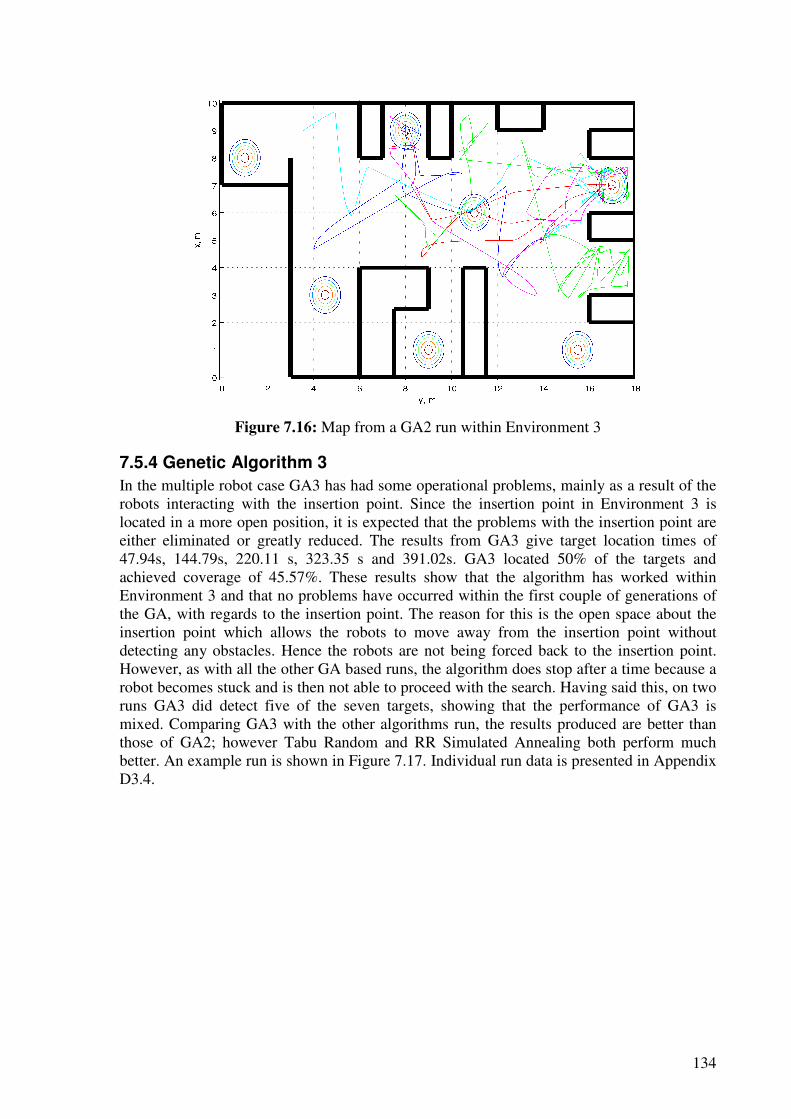
134
Figure 7.16: Map from a GA2 run within Environment 3
7.5.4 Genetic Algorithm 3
In the multiple robot case GA3 has had some operational problems, mainly as a result of the robots interacting with the insertion point. Since the insertion point in Environment 3 is located in a more open position, it is expected that the problems with the insertion point are either eliminated or greatly reduced. The results from GA3 give target location times of 47.94s, 144.79s, 220.11 s, 323.35 s and 391.02s. GA3 located 50% of the targets and achieved coverage of 45.57%. These results show that the algorithm has worked within Environment 3 and that no problems have occurred within the first couple of generations of the GA, with regards to the insertion point. The reason for this is the open space about the insertion point which allows the robots to move away from the insertion point without detecting any obstacles. Hence the robots are not being forced back to the insertion point. However, as with all the other GA based runs, the algorithm does stop after a time because a robot becomes stuck and is then not able to proceed with the search. Having said this, on two runs GA3 did detect five of the seven targets, showing that the performance of GA3 is mixed. Comparing GA3 with the other algorithms run, the results produced are better than those of GA2; however Tabu Random and RR Simulated Annealing both perform much better. An example run is shown in Figure 7.17. Individual run data is presented in Appendix D3.4.
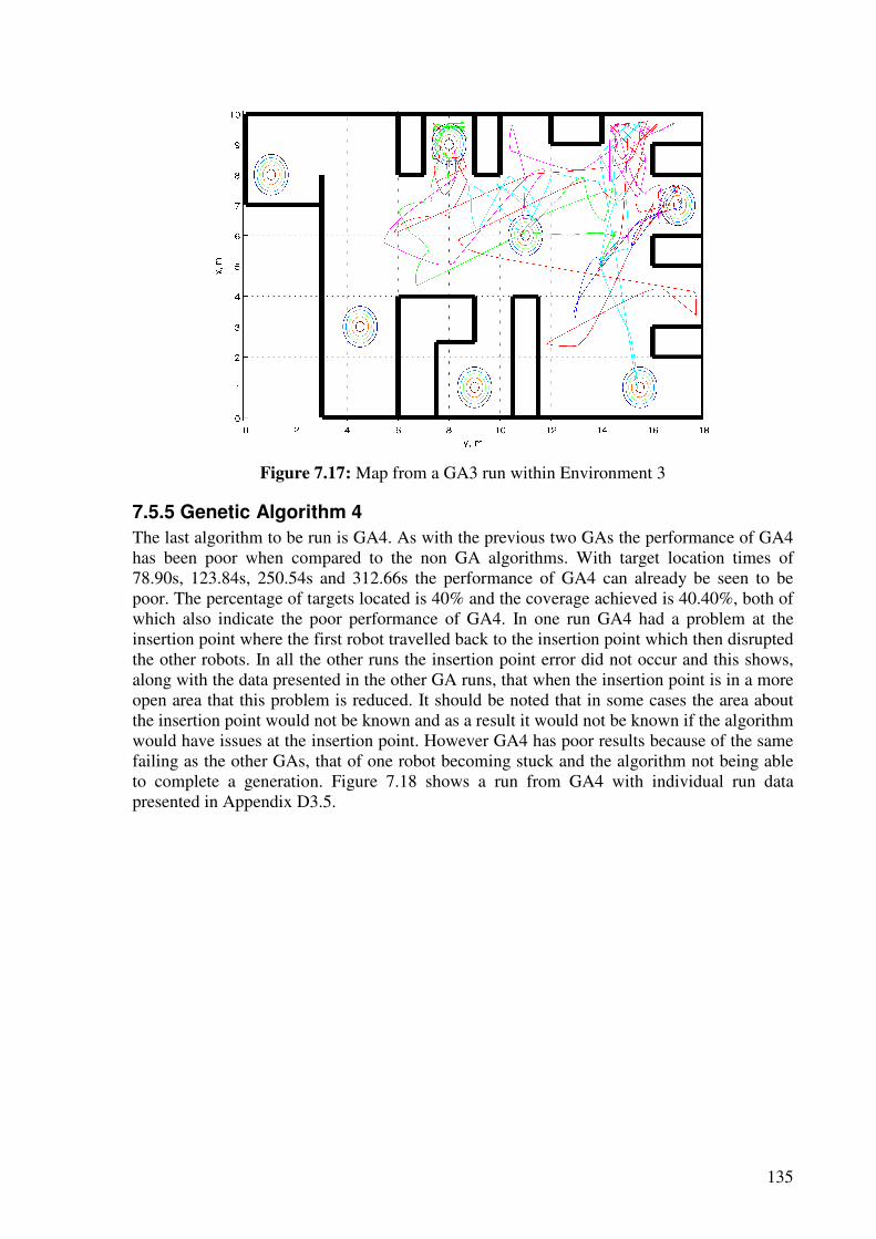
135
Figure 7.17: Map from a GA3 run within Environment 3
7.5.5 Genetic Algorithm 4
The last algorithm to be run is GA4. As with the previous two GAs the performance of GA4 has been poor when compared to the non GA algorithms. With target location times of 78.90s, 123.84s, 250.54s and 312.66s the performance of GA4 can already be seen to be poor. The percentage of targets located is 40% and the coverage achieved is 40.40%, both of which also indicate the poor performance of GA4. In one run GA4 had a problem at the insertion point where the first robot travelled back to the insertion point which then disrupted the other robots. In all the other runs the insertion point error did not occur and this shows, along with the data presented in the other GA runs, that when the insertion point is in a more open area that this problem is reduced. It should be noted that in some cases the area about the insertion point would not be known and as a result it would not be known if the algorithm would have issues at the insertion point. However GA4 has poor results because of the same failing as the other GAs, that of one robot becoming stuck and the algorithm not being able to complete a generation. Figure 7.18 shows a run from GA4 with individual run data presented in Appendix D3.5.
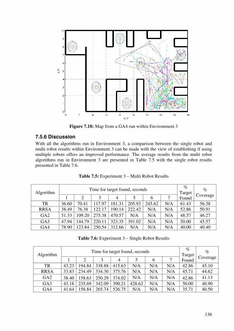
136
Figure 7.18: Map from a GA4 run within Environment 3
7.5.6 Discussion
With all the algorithms run in Environment 3, a comparison between the single robot and multi robot results within Environment 3 can be made with the view of establishing if using multiple robots offers an improved performance. The average results from the multi robot algorithms run in Environment 3 are presented in Table 7.5 with the single robot results presented in Table 7.6.
Table 7.5: Experiment 3 – Multi Robot Results
Time for target found, seconds Algorithm
1 2 3 4 5 6 7
% Target Found
% Coverage
TR 36.60 70.41 117.97 181.31 205.93 245.62 N/A 61.43 56.38 RRSA 38.49 76.38 122.17 190.14 222.42 N/A N/A 52.86 50.91 GA2 51.33 109.20 275.38 470.57 N/A N/A N/A 48.57 46.27 GA3 47.94 144.79 220.11 323.35 391.02 N/A N/A 50.00 45.57 GA4 78.90 123.84 250.54 312.66 N/A N/A N/A 40.00 40.40
Table 7.6: Experiment 3 – Single Robot Results
Time for target found, seconds Algorithm
1 2 3 4 5 6 7
% Target Found
% Coverage
TR 43.23 194.84 338.88 415.63 N/A N/A N/A 42.86 45.10 RRSA 33.83 234.49 334.30 375.76 N/A N/A N/A 45.71 44.62 GA2 38.40 158.63 250.29 374.02 N/A N/A N/A 42.86 41.13 GA3 43.18 235.69 342.09 390.21 428.62 N/A N/A 50.00 40.90 GA4 41.64 158.84 265.74 526.75 N/A N/A N/A 35.71 40.50
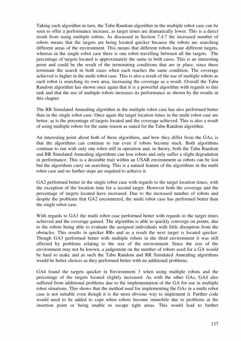
137
Taking each algorithm in turn, the Tabu Random algorithm in the multiple robot case can be seen to offer a performance increase, as target times are dramatically lower. This is a direct result from using multiple robots. As discussed in Section 7.4.7 the increased number of robots means that the targets are being located quicker because the robots are searching different areas of the environment. This means that different robots locate different targets, whereas in the single robot case there is one robot travelling between all the targets. The percentage of targets located is approximately the same in both cases. This is an interesting point and could be the result of the terminating conditions that are in place, since these terminate the search in both cases when each reaches the same condition. The coverage achieved is higher in the multi robot case. This is also a result of the use of multiple robots as each robot is searching its own area, increasing the coverage as a result. Overall the Tabu Random algorithm has shown once again that it is a powerful algorithm with regards to this task and that the use of multiple robots increases its performance as shown by the results in this chapter. The RR Simulated Annealing algorithm in the multiple robot case has also performed better than in the single robot case. Once again the target location times in the multi robot case are better, as is the percentage of targets located and the coverage achieved. This is also a result of using multiple robots for the same reason as stated for the Tabu Random algorithm. An interesting point about both of these algorithms, and how they differ from the GAs, is that the algorithms can continue to run even if robots become stuck. Both algorithms continue to run with only one robot still in operation and, in theory, both the Tabu Random and RR Simulated Annealing algorithms can lose robots and only suffer a slight degradation in performance. This is a desirable trait within an USAR environment as robots can be lost but the algorithms carry on searching. This is a natural feature of the algorithms in the multi robot case and no further steps are required to achieve it. GA2 performed better in the single robot case with regards to the target location times, with the exception of the location time for a second target. However both the coverage and the percentage of targets located have increased. Due to the increased number of robots and despite the problems that GA2 encountered, the multi robot case has performed better than the single robot case. With regards to GA3 the multi robot case performed better with regards to the target times achieved and the coverage gained. The algorithm is able to quickly converge on points, due to the robots being able to evaluate the assigned individuals with little disruption from the obstacles. This results in quicker RRs and as a result the next target is located quicker. Though GA3 performed better with multiple robots in the third environment it was still affected by problems relating to the size of the environment. Since the size of the environment may not be known, a judgement on the number of robots used for a GA would be hard to make and as such the Tabu Random and RR Simulated Annealing algorithms would be better choices as they performed better with no additional problems. GA4 found the targets quicker in Environment 3 when using multiple robots and the percentage of the targets located slightly increased. As with the other GAs, GA4 also suffered from additional problems due to the implementation of the GA for use in multiple robot situations. This shows that the method used for implementing the GAs in a multi robot case is not suitable even though it is the most obvious way to implement it. Further code would need to be added to cope when robots become immobile due to problems at the insertion point or being unable to escape tight areas. This would lead to further
138
complications with regards to code implementation and it is unknown if a performance increase would be achieved. With regards to the performance over all the environments, Tabu Random and RR Simulated Annealing algorithms have performed consistently better in the multi robot case when compared to the single robot case. The GAs have given a mixed set of results. In the smaller more constrained environments the GAs have not performed well. However in the bigger more open environment, the results produced indicate that multi robot GAs perform well.
7.6 Review of Results
Throughout this chapter the comparison between the multi robot results and the single robot results has been carried out. This section provides a review of both sets of results and suggests a suitable algorithm for use in the scenario described. It was established in Chapter 6 that the algorithms discussed in Chapter 5 can be implemented in the task described, with the exception of the HillClimbing algorithm. This conclusion is backed up by the evidence provided in Chapter 6. With regards to the best performing algorithms in a single robot case, the conclusion was that algorithms that contain both a high random element and some structure to the selection of points perform well. The algorithms in this work that show this are the Tabu Random and RR Simulated Annealing algorithms and GA2, GA3 and GA4. From the evidence in Chapter 6 it was suggested that the Tabu Random algorithm was the best choice for use in a single robot case. Over all the runs the Tabu Random algorithm performed well. It is also simple to implement, allowing implementation on a wide range of platforms. The results in Chapter 7 have provided evidence of how the algorithms run when implemented in a multi robot case. The conclusions that can be drawn from the data presented give a mixed picture of what can be achieved in a multi robot case. The first point to note is the failure of the Genetic Algorithms when implemented in the way described in this chapter. The Genetic Algorithms performed well in the single robot case but, due to problems associated with the individual robots becoming stuck within the environment, the performance in the multi robot case was poor in comparison. However it was shown that in an open environment, such as that of Environment 3, an improvement does exist. With regards to the Tabu Random and Simulated Annealing algorithms the multi robot case did provide improvements within Environments 2 and 3. The results from Environment 1 were similar. The Tabu Random results are compared in Table 7.7 and the Simulated Annealing results can be found in Table 7.8. It can be seen in both of the tables that the improvements gained within Environment 1 are similar. This would indicate that it would be better to run a single robot within this environment, as the deployment of one robot would be simpler than the deployment of five. An improvement is seen in both the multiple robot runs in Environments 2 and 3. This shows that as the environment either becomes more complicated or becomes larger then multiple robots should be deployed. In both the single robot and multi robot cases the Tabu Random algorithm has performed well. This would indicate that the Tabu Random algorithm would be a good choice for implementation in a practical scenario.
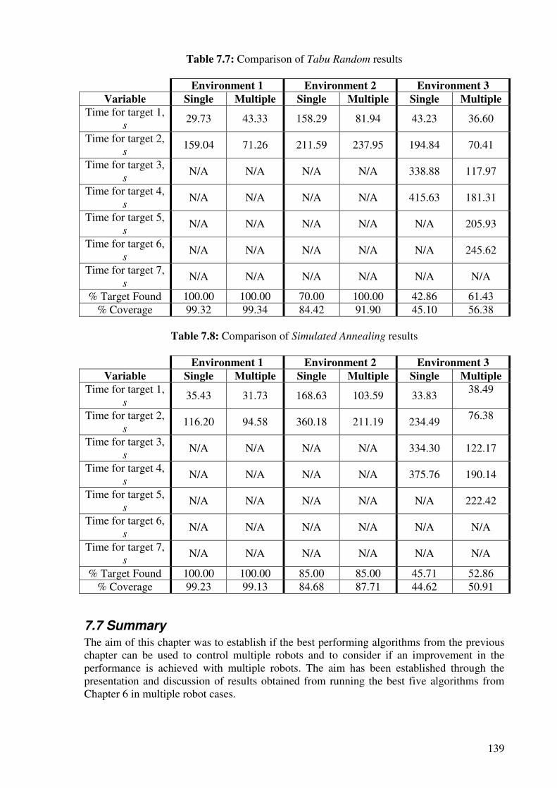
139
Table 7.7: Comparison of Tabu Random results
Environment 1 Environment 2 Environment 3
Variable Single Multiple Single Multiple Single Multiple
Time for target 1, s
29.73 43.33 158.29 81.94 43.23 36.60
Time for target 2, s
159.04 71.26 211.59 237.95 194.84 70.41
Time for target 3, s
N/A N/A N/A N/A 338.88 117.97
Time for target 4, s
N/A N/A N/A N/A 415.63 181.31
Time for target 5, s
N/A N/A N/A N/A N/A 205.93
Time for target 6, s
N/A N/A N/A N/A N/A 245.62
Time for target 7, s
N/A N/A N/A N/A N/A N/A
% Target Found 100.00 100.00 70.00 100.00 42.86 61.43 % Coverage 99.32 99.34 84.42 91.90 45.10 56.38
Table 7.8: Comparison of Simulated Annealing results
Environment 1 Environment 2 Environment 3
Variable Single Multiple Single Multiple Single Multiple
Time for target 1, s
35.43 31.73 168.63 103.59 33.83 38.49
Time for target 2, s
116.20 94.58 360.18 211.19 234.49 76.38
Time for target 3, s
N/A N/A N/A N/A 334.30 122.17
Time for target 4, s
N/A N/A N/A N/A 375.76 190.14
Time for target 5, s
N/A N/A N/A N/A N/A 222.42
Time for target 6, s
N/A N/A N/A N/A N/A N/A
Time for target 7, s
N/A N/A N/A N/A N/A N/A
% Target Found 100.00 100.00 85.00 85.00 45.71 52.86 % Coverage 99.23 99.13 84.68 87.71 44.62 50.91
7.7 Summary
The aim of this chapter was to establish if the best performing algorithms from the previous chapter can be used to control multiple robots and to consider if an improvement in the performance is achieved with multiple robots. The aim has been established through the presentation and discussion of results obtained from running the best five algorithms from Chapter 6 in multiple robot cases.
140
The results, over all the runs, have shown that using multiple robots has increased the performance of both the Tabu Random and RR Simulated Annealing algorithms and due to the nature of the method used to implement the algorithms, both algorithms are able to cope with the loss of individual robots. This is not the case with the implementation used for the GAs. GA2, GA3 and GA4 all suffered from issues in each environment, mainly as a result of the GA needing to rely on all of the robots operating successfully in the environment. The results have shown that this does not happen and in all the GA runs it can be seen that a robot becomes stuck and as a result the algorithm is forced to stop. It was also established that the algorithm that has performed best overall is the Tabu Random algorithm. This algorithm performed well in both the single and multi robot cases and showed no degradation in performance when any individual robots became immobile within the multiple robot case. A further point that came from the results presented in this chapter is that the size of the environment affects the useable number of robots. When the multi robot Tabu Random and RR Simulated Annealing algorithms were run in Environment 1, the results achieved were similar to those achieved by the single robot runs in the same environment. This shows that the size of the environment has an impact on the number of robots that can be used to search it.
141
Chapter 8
Conclusions and Further Work
8.1 Conclusions
The task of locating survivors within environments during USAR can be dangerous and puts the lives of both the survivors and rescue workers at risk. This work proposed the use of robots to search environments under the control of search algorithms. The reasoning behind this approach is that search algorithms are used in multiple fields of research and in industry to locate optimal points within a search space. If a simple method of identifying a survivor was achievable, such as the detection of body heat, and a unique point, or range of points, existed within this identification, an optimal point can be declared. It can then be shown that, in theory, the location of a survivor in an environment, which is the algorithm’s search space, can be achieved by search algorithms. The aim of the work presented in this thesis was to establish if search algorithms could be used to search for survivors within an environment. This work was to also select algorithms which performed the task well and to establish if the use of multiple robots resulted in a better performance over the single robot search. Additional objectives included the development of both a mathematical model of a mobile
robot and a navigation and control system to enable the testing and operation of the search algorithms. The first part of this work was concerned with the development of a mathematical model of a suitable mobile robot for use in USAR. Chapter 3 presented the development of the model and introduced the validation of this model. The model developed is a six-degree-of-freedom model with actuators. The dynamics and kinematics of the model were considered along with the dynamics of the actuators. The inclusion of the actuators gave a complete model of a mobile robot. A further stage of the model development was the validation of the model. Two methods of validation were used: Analogue Matching and Least Mean Squares. The validation shows that the model is a close representation of the real robot and as such the results from the simulation are a good approximation to what the results from a real robot would be. The search algorithms are designed to generate points to which the robot will travel to. However a method of ensuring the robot travels to the requested points accurately is required. To accomplish this task a navigation and control system was developed in Chapter 4. The navigation and control system was made up of three parts: the navigation system, the control system and an obstacle avoidance routine. The navigation system consisted of a Line
of Sight Autopilot which generated the heading the robot should take to reach the next assigned point. A method of ensuring the robot travelled along the correct heading and at a suitable speed was needed. This was done by the control system. The control system took, as input, the heading generated by the navigation system and the desired speed and from these generated suitable actuator voltages which enabled the robot to travel to the assigned points. A suitable control methodology was required that would efficiently and accurately maintain both the speed and heading. Chapter 4 presented three methods of control for consideration: Proportional-Integral-Derivative, Pole Placement and Sliding Mode. Each controller was tested in simulation on the modelled robot in a series of experiments and the results were
142
compared using measurements taken from the data. The measurements taken allowed a comparison of the controllers based on the average tracking error, average steady state
error, rise time, charge drawn from the battery and motion control. After this comparison was carried out it was found, with regards to the modelled robot and the implementation of the controllers in this work, that the Pole Placement controller was the most suitable control method to be implemented for this task. The Pole Placement controller performed better than both the Proportional-Integral-Derivative and Sliding Mode controllers within the experiments designed in this work. A further aspect of the navigation and control system was the obstacle avoidance routine. When operating in all but the simplest of environments obstacles will exist and the controller needs to respond to the detection of obstacles. This work considered two methods of obstacle avoidance. A method designed to navigate around
the obstacle and a reactive method. The first method mentioned is designed to navigate round obstacles by following a set pattern. The second method simply replaces the desired point with a randomly selected point. It was found that, taking into consideration that time is an important variable in this work, the reactive approach was the best method. Though the reactive method did not always get to the required point the time saved by not going round an obstacle was found to be more desirable. Chapter 5 presented and discussed the search algorithms chosen for implementation in this work. The search algorithms were chosen as they are established and popular methods. Traditional search algorithms that were chosen were Lawnmower, a form of the Exhaustive search, Random, HillClimbing and Random Restart HillClimbing. Modern search algorithms that were considered were based on Tabu search, with Tabu Random and Tabu Random
Restart HillClimbing being variants that were investigated, Random Restart Simulated
Annealing and four variations of the Genetic Algorithm. Each of these algorithms was discussed and how they are implemented presented. As part of the discussion on the search algorithms, various functions that are common to all the experimental runs was presented. These functions allow the robot to carry out the search and provide a means of comparing each search algorithm. How the temperature is tracked was presented along with the implementation of the constant search. Since coverage is a method of comparison it was discussed with reference to this work. The robot is required to detect targets. How this is achieved was discussed. The next stage in this work provided results and the analysis of the algorithms run. The first set of results, presented in Chapter 6 and Appendix C, clearly indicated that the search algorithms could be used to provide points which allow a single robot to search for targets within a given environment. It was found that algorithms with a high random element and a structure to the selection of points provided the best results. The high random element enables the search to achieve a wide coverage within the environment. Having a structure to select the next point is also important. Whether this structure allows the robot to converge on a point (RR Simulated Annealing, GA2, GA3 and GA4) or is simply a list of points that are not to be selected (Tabu Random) is not important, though it is acknowledged that the algorithms which converge can, on occasion, find targets quicker. The algorithms which performed best, with regards to the single robot results presented in this work, are the Tabu
Random and RR Simulated Annealing algorithms, and, GA2, GA3 and GA4. Each of these algorithms achieved desirable performances over all the environments that they were tested in and, through the results, showed to be suitable algorithms for selection with regards to the implementation used in this work and in the task described. Over all the runs in a single robot case the Tabu Random algorithm performed the best.
143
Since it was established that the algorithms are suitable for the task described and five of the algorithms were deemed to stand out from the others, based on the results presented in this work, an investigation into the impact of having multiple robots searching can be done. The algorithms were implemented to allow the five robots to be run. With regards to the RR
Simulated Annealing algorithm this implementation created a decentralised control algorithm, as each robot ran an independent version of the algorithm. The Tabu Random algorithm had a global Tabu List which each robot added to and referenced. This had a centralised approach to the implementation of the algorithm. The GAs were also implemented with a centralised approach. Within each GA each robot searched for an individual in the population and once all the individuals were evaluated the current generation was evaluated. The results presented in Chapter 7 offer a mixed answer to the application of multiple robots. Results from Chapter 7 show that the Tabu Random and RR
Simulated Annealing algorithms both saw improvements when implemented with multiple robots. It was also noted that the performance of these two algorithms did not degrade when robots fail. This would be an important aspect within a practical application of the ideas in this work, as the robots may fail or become stuck when used in the field. However the multiple robot implementation of the GAs failed to show any improvement over all the runs. GA2, GA3 and GA4 all suffered from issues relating to the implementation of the algorithm. In each environment the robots became stuck. This was shown to affect the overall performance of the algorithm. The reason for this is that the GA is reliant on all the robots operating successfully in the environment. The results indicate that this cannot be taken for granted and hence the GAs will be prone to failure with the current method of implementation. It was also noted in Chapter 7 that the size of the environment may affect the number of robots that can be used to carry out the search. A slight increase in performance was seen for the Tabu Random and RR Simulated Annealing algorithms in the smaller environments, but the performance increase was only slight. The Tabu Random algorithm was shown to be the best algorithm within a multi robot case. This work proposed the use of autonomous robots to search environments under the control of search algorithms. Since lives are at risk within USAR scenarios, the robot or team of robots would need to be able to search an environment as thoroughly and quickly as they can. This work has found that, with regards to the results shown throughout this thesis, the Tabu Random algorithm would be a suitable search algorithm, for both single robot and multiple robot searches. The Tabu Random algorithm achieved good coverage and located a large percentage of the targets within the environments. The targets were also located in a reasonable time. This algorithm also showed the ability to continue working even when individual robots in the team become immobile. This would be beneficial to the area of USAR when using robots. The application of either a single robot or team of robots under the control of the Tabu Random algorithm may prove to be a useful tool for any team or emergency service that is required to search environments for people. Though some technological challenges still exist, the concept explored in this work has the potential to save lives.
8.2 Further Work
This work set out to establish if search algorithms could be implemented on a mobile robot or group of mobile robots to carry out a search of an environment. The results indicate that this is possible and that the Tabu Random algorithm is best suited to the task when implemented in the way done in this work. However this work can be taken further. Further work, which is based on the work presented here, is suggested next.
144
8.2.1 Hybrid Algorithms
The first area of interest would be the implementation of hybrid algorithms. The Tabu
Random and the Tabu Random Restart HillClimbing algorithms were both hybrid algorithms as they are created by the fusion of two different algorithms. This concept could be taken further to enable the algorithms to be improved and, in turn, improve the results. There exist many different algorithms that can be fused together, but based on the results gathered throughout this work the following hybrid algorithms would be worth further investigation: Global Tabu with additional algorithm and Tabu Random with HillClimbing. 8.2.1.1 Global Tabu with additional algorithm
The first hybrid algorithm is more a concept for implementation than a hybrid algorithm. The Tabu element was found to be a powerful function when implemented and provided one of the best algorithms. The operation of the Tabu element was based on maintaining a list of points that could not be selected again until after a certain time. This concept could be extended to provide a Global Tabu list. One problem that is present in all the algorithms is that once a target is located the algorithm is still attracted to it. Since the algorithm is still attracted to the target, the robot wastes time revisiting it and some algorithms cannot escape the attraction of the target. One method of dealing with this is to maintain a Global Tabu list that is only updated when a target is found. In doing this the targets are tracked in one list and the algorithm can refer to this when selecting the next point to go to. To further improve this, once a target is located a Tabu radius can be introduced around it to stop the robot coming within a set range of a target, aiding the algorithm’s ability to escape target points. This would aid all the algorithms, as it would increase the coverage, as areas that have been searched which contain targets, would be off limits. As stated previously, with increased coverage the chances of locating targets is increased. It can be seen that this could have a dramatic affect on the ability of the robot to search environments. An issue that would be created by implementing the Global Tabu is if the robot became stuck within an area that it cannot be moved from as it is surrounded by either obstacles or located targets. In this case a conditional Tabu would need to be created. The algorithm cannot direct the robot to a located target unless no other path exists. In essence the algorithms would be allowed to travel through a Global Tabu zone if necessary. This hybrid algorithm could be added onto any of the algorithms that have been studied but it should be first implemented on the best performing algorithms. 8.2.1.2 Tabu Random with HillClimbing
The second hybrid algorithm that should be investigated is a Tabu Random with
HillClimbing algorithm. It has been shown that the Tabu Random algorithm performs well within both the single robot and multi robot cases, but with the addition of a HillClimbing element the performance could be increased. The Tabu Random algorithm operates as described in this work, however when an increase in temperature is detected the algorithm would then switch to the HillClimbing algorithm which, as results in this work suggest, would bring the robot to the target point quickly, if one exists in the immediate vicinity. Once either a target point is detected or no higher temperature point is detected the algorithm would then switch back to the Tabu Random element of the algorithm and continue the search of the environment. This algorithm would, in theory, improve the target location times, hence the overall performance of the algorithm would be improved. This algorithm would incorporate both elements that the results suggested are needed to search an environment and locate targets quickly: a high random element, implemented by the Tabu
Random and a structured approach to the location of targets, the HillClimbing algorithm. This algorithm is similar to the way the RR Simulated Annealing works, which also
145
performed very well, but is more direct when locating the targets points. With the inclusion of a Global Tabu element this algorithm could perform exceptionally well.
8.2.2 Improved Robotic Platform
Another area of further work would be an improved robotic platform. To keep within the ethos of this work a simple disposable robot was used to implement the algorithms on. In doing this a number of problems were encountered. The obstacle avoidance had to be implemented in a very simple way and only one temperature sensor was used giving a very limited field of view. To include additional sensors would provide the means of improving the obstacle avoidance, meaning that the robot will not become stuck in tight areas. Mapmaking would become a realistic concept and more information from the environment can be retrieved allowing better direction from the algorithms. With the addition of more sensors, more processing will be required which will increase the size of the robot, which will mean that the robot will require more power to run. However with the additional data that more sensors could provide, an improved platform would be a good path of investigation. With the addition of more obstacle detection sensors the robot would spend less time avoiding obstacles. Also the chance of becoming stuck would be reduced as it would be able to carry out path planning to avoid obstacles. When the robot becomes stuck, a suite of obstacle sensors would enable the robot to detect a path out from its current location. Both of these would give the robot more time to carry out the search. Also, with more sensors the ability to create a map of the environment becomes viable. With a map the rescue workers would have a better idea of what the environment was like and provide them a route to any survivors located. A map would also provide the robot the ability to path plan routes through the environment once an area had been mapped. The addition of more temperature sensors would also greatly enhance the search of an environment. As it is the robot has a limited cone it can search while it is travelling between points. With additional sensors the robot could carry out a 360° scan of the area it passes through, increasing the chance of locating survivors.
8.2.3 Decentralised Control
As this work stands the method used by each algorithm is, in essence, a centralised method, though the RR Simulated Annealing multi robot algorithm can be viewed as a decentralised method. As the robot moves it transmits information back to a base station and then awaits instructions back from it. Many of the algorithms could be run on an improved robot. This would mean that the robot could be instructed to search an environment and then the only time it contacts a base station is when a target is located. This would help with regards to the reality of the communication in the environments this work is designed for. Also with each robot (in a multiple robot case) working independently, better results may be achieved by algorithms as they do not have to wait for other robots to complete a task. This could replicate a single robot performance but in a multiple robot case. The area of decentralised control has the possibility of providing improvements to the search algorithms.
8.2.4 Varying the Number of Robots
It was shown in Chapter 7 that the number of robots used in an environment may affect the performance of the algorithm run. The results indicated that in small environments a single robot may provide results that are equal to or better than those achieved by a multiple robot search. The reverse may also be true; as the environment gets bigger the number of robots used to search the environment should be increased. With the simulation used in this work it would be possible to research a range of different robot numbers easily and within different environments.
146
References
Åström, K., and Hägglund, T., (1995), PID Controllers: Theory, Design, and Tuning 2nd edition, Instrument Society of America Albagul, A., and Wahyudi, (2004), “Dynamic Modelling and Adaptive Traction Control for Mobile Robots”, International Journal of Advanced Robotic Systems, Vol. 1, No 3, pp. 149-154 Alfaro-Cid, M.E., (2003), Optimisation of Time Domain Controllers for Supply Ships Using
Genetic Algorithms and Genetic Programming, Phd Thesis, Department of Electronic and Electrical Engineering, University of Glasgow Alfaro-Cid, M.E., McGookin, E.W. and Murray-Smith, D.J., (2006) “GA-optimised PID and pole placement real and simulated performance when controlling the dynamics of a supply ship” IEE Proceedings Control Theory and Applications, Vol. 153, Issue 2 Anagnostopoulos, A., Van Hentenryck P. and Vergados, Y., (2006) “A simulated annealing approach to the traveling tournament problem” Journal of Scheduling, Springer Netherlands, Vol. 9, No. 2, pp 177-193 Astolfi, A. (2006), “Stabilization of Nonholonomic Systems”, Autonomous Mobile Robots:
Sensing, Control, Decision Making and Applications, Taylor and Francis Group Balakrishna, R. and Ghosal, A., (1995), “Modeling of Slip for Wheeled Mobile Robots”, IEEE Transactions on Robotics and Automation, Vol. 11, No 1, pp. 126-132 Barshan, B. and Durrant-Whyte, H.F., (1995), “Inertial Navigation Systems for Mobile Robots”, IEEE Transactions on Robotics and Automation, Vol. 11, No. 3, June Bennet, S., (1996), “A Brief History of Automatic Control”, IEEE Control Systems
Magazine, Vol. 16, No 3, pp 17-25 Birk, A., and Carpin, S., (2006), “Rescue Robotics – A Crucial Milestone on the Road to Autonomous Systems”, Advanced Robotics Journal, 20 (5), VSP International Science Publishers Birk, A., Pathak, K., Schwertfeger, S. and Chonnaparamutt, W., (2006) “The IUB Rugbot: an intelligent, rugged mobile robot for search and rescue operations”, IEEE International
Workshop on Safety, Security, and Rescue Robotics, IEEE Press Bisgaard, M., Vinther, D., Ostergaard, K., Bendsten, J. and Izadi-Zamanabadi, R., (2005), “Sensor Fusion and Model Verification for a Mobile Robot”, Proceedings of the 16
th
IASTED International Conference Modelling and Simulation, pp. 106-111 Blitch, J.G., (1996), “Artificial Intelligence Technologies for Robot Assisted Urban Search and Rescue”, Expert Systems With Applications, Vol. 11, No 2, pp. 109-124
147
Bohachevsky, I.O, Johnson, M.E. and Stein, M.L., (1986), “Generalised Simulated Annealing for Function Optimisation”, Tehnometerics, Vol. 28, No. 3, pp 209-217 Braga, N.C., (2002), Robotics, Mechtronics, and Artificial Intelligence, Newnes Buchmann, I., (2000), Batteries in a Portable World: A Handbook on Rechargeable
Batteries for Non-Engineers, Cadex Electronics Inc, 2nd Edition Burke, T. and Durrant-Whye, H.F., (1993), “Kinematics for Modular Wheeled Mobile Robots”, Proceedings of the 1993 IEEE/RSJ International Conference on Intelligent Robots
and Systems, pp. 1279-1286 Čapek, K., 1920, R.U.R, English Translation: Majer, P. and Porter, C., Čapek Four Plays, Methuen Publishing, London, ISBN: 0413771903 Carlson, J., and Murphy, R.R., (2005) “How UGVs physically fail in the field”, IEEE Transactions on Robotics, Vol. 21, No. 3, pp. 423-437 Casper J., Murphy R.R. and Micire M., (2000), "Issues in Intelligent Robots for Search and Rescue", SPIE Ground Vehicle Technology II, Orlando, Florida Cetinkunt, S., (2007), Mechatronics, John Wiley & Sons, Inc Cheng, C.K., and Leng, G., (2004), “Cooperative Search Algorithm for Distributed Autonomous Robots”, Proceedings of 2004 IEEE/RSJ International Conference on
Intelligent Robots and Systems, pp.394-399 Chow, J.H. and Sanchez-Gasca, J.J. (1989) “Pole-placement designs of power system stabilizers” IEEE Transactions on Power Systems, Vol. 4, Issue 1, pp 271-277 Cook, M.V., (1997), Flight Dynamic Principles, Butterworth Heinemann CRASAR, (2008), http://www.crasar.org/MainFiles/, Home Page for Center of Robotic
Assisted Search and Rescue, 24/09/2008 DeCarlo, R.A., Zak, S.H. and Matthews, G.P, (1988), “Variable Structure Control of Nonlinear Multivariable Systems: A Tutorial”, Proceedings of the IEEE, Vol. 76, No 3, pp. 212-232 DeJong, K.A., (1975), An Analysis of the Behaviour of a Class of Genetic Adaptive Systems, PhD thesis, University of Michigan Dollarhide, R.L. and Agah, A., (2003), “Simulation and Control of Distributed Robot Search Teams”, Computers and Electrical Engineering, 29, 625-642 Dorf, R.C. and Bishop, R.H., (2005), Modern Control Systems, Pearson Prentice Hall, 10th edition, International edition Dutton, K., Thompson, S. and Barraclough, B., (1997), The Art of Control Engineering, Addison-Wesley
148
Edwards, C. and Spurgeon, S.K., (1998), Sliding Mode Control: Theory and Applications, Taylor and Francis Ellis, C. (1993), “A Bluffers Guide to Genetic Algorithms”, Engineering Design Newsletter, SERC, Summer Fahimi, F., (2007), “Sliding-Mode Formation Control for Underactuated Surface Vessels”, IEEE Transaction on Robotics, Vol. 23, No 3, pp. 617-622 Frankin, G.F., Powell, J.D. and Emami-Naeini, A., (1991). Feedback Control of Dynamic
Systems, 2nd
Edition, Addison Wesley Fossen, T.I., (2002), Marine Control Systems: Guidance, Navigation, and Control of Ships,
Rigs and Underwater Vehicles, Marine Cybernetics Fossen, T.I., (1994), Guidance and Control of Ocean Vehicles, Wiley & Sons Ltd Gazi, V., (2005), “Swarm Aggregations Using Artificial Potentials and Sliding-Mode Control”, IEEE Transactions on Robotics, Vol. 21, No 6, pp. 1208-1214 Ge, S.S., and Lewis, F.l., eds, (2006), Autonomous Mobile Robots: Sensing, Control,
Decision Making and Applications, Taylor and Francis Group Gendreau, M., (2003), “Introduction to Tabu Search”, Handbook of Metaheuristic, International Series in Operations Research & Management, eds. Glover, G., Kochenberger, G.A., Springer, pp.37-54 Glover, F. (1989), “Tabu Search: Part 1”, ORSA J. of Computing, 2, No 1, pp190-206 Glover, F., (1986), “Future Paths for Integer Programming and Links to Artificial Intelligence”, Comput’ & Ops’ Res., Vol. 13, No 5, pp. 533-549 Goldberg, D., (1989), Genetic Algorithms in Searching, Optimisation and Machine
Learning, Addison Wesley, Reading, MA Granosik, G. and Borenstein, J., (2005) “Integrated Joint Actuator for Serpentine Robots”, IEEE/ASME Transactions on Mechatronics, Vol. 10, No 5, October Gray, G., (1992), Development and Validation of Nonlinear Models for Helicopter
Dynamics, PhD Thesis, Department of Electronic and Electrical Engineering, University of Glasgow
Hatta, K., Wakabayashi, S. and Koide, T., (2001), “Adaptation of Genetic Operators and Parameters of a Genetic Algorithm Based on the Elite Degree of an Individual”, Systems and
Computers in Japan, Vol. 31, No 1, pp. 29-37
Healey, A.J. and Kim, J., (2000), “Control and Random Searching with Multiple Robots”, Proceedings of the 39
th IEEE Conference on Decision and Control, pp. 340-345
149
Healey, A.J. and Leinard, D., (1993), “Multivariable Sliding Mode Control for Autonomous Diving and Steering of Unmanned Underwater Vehicles”, IEEE Journal of Oceanic
Engineering, Vol. 18, No. 3, pp 327-339 Hertz, A., Taillard, E., De Werra, D., “A Tutorial on Tabu Search”, Proc. of Giornate di
Lavoro AIRO’95, Entreprise Systems: Management of Technological and Organizational
Changes, pp. 13-24 Hoerner, S.F., (1965), Fluid-dynamic drag: practical information on aerodynamic drag and
hydrodynamic resistance, Brick Town, New Jersey Holland, J.H., (1992), “Genetic Algorithms”, Scientific American, July Holland, J.H., (1975), Adaptation in Natural and Artificial Systems, University of Michigan Press Hong, F., Ge, S.S., Lewis, F.L. and Lee, T.H., (2006), “Adaptive Neural-Fuzzy Control of Nonholonomic Mobile Robots”, Autonomous Mobile Robots: Sensing, Control, Decision
Making and Applications, Taylor and Francis Group Hong, T., Wang, H. and Chen, W., (2000), “Simultaneously Applying Multiple Mutation Operators in Genetic Algorithms”, Journal of Heuristics, 6, pp. 439-455 Ichbiah, D., (2005), Robots: From Science Fiction to Technological Revolution, Harry N. Abrams, Inc, New York IRSI, (2008), http://www.rescuesystem.org/, Homepage for the International Rescue System
Institute, 24/09/2008 Jellet, J., 1872, Theory of Friction, McMillian & Co Jennings, J., Whelan, G. and Evans, W.F., (1997), “Cooperative Search and Rescue with a Team of Mobile Robots”, ICAR, Monterey, CA, July 7-9 Johnson, J. and Picton, P., (1995), Mechatronics: Designing Intelligent Machines Volume 2:
Concepts in Artificial Intelligence, Butterworth Heinemann and The Open University Kautsky, J., Nichols, N.K. and Van Doorens, P., (1985), “Robust Pole Assignment in Linear State Feedback”, International Journal of Control, Vol. 41, No 5, pp1129-1155 Kelly, A. and Rinnie, K., (2005), “Control of dc-dc converters by direct pole placement and adaptive feedforward gain adjustment” Applied Power Electronics Conference and Exposition, Twentieth Annual IEEE, Vol. 3 pp.1970-1975 Khoo, K.G. and Suganthan, P.N., (2002), “Evaluation of Genetic Operators and Solution Representations for Shape Recognition by Genetic Algorithms”, Pattern Recognition Letters, 23, pp. 1589-1597 Kirkpatrick, S., (1984), “Optimization by Simulated Annealing: Quantitative Studies”, Journal of Statistical Physics, Vol. 34, Nos. 5/6, pp. 975-986
150
Kirkpatrick, S., Gelatt, C.D.Jr and Vecchi, M.P., (1983), “Optimization by Simulated Annealing”, Science, Vol. 220, No 4598, pp.671-680 Kitano, H., Tadokoro, S., Noda, I., Matsubara, H., Takahashi, T., Shinjou, A. and Shimada, S., (1999), “RoboCup Rescue: Search and rescue in Large-Scale Disasters as a Domain for Autonomous Agents Research”, Proceedings of IEEE Conference on Man, Systems, and
Cybernetics (SMC-99)
Kitano, H., Asada, M., Kuniyoshi, Y., Noda, I., Osawa, E. and Matsubara, H., (1997), “Robocup A Challenge AI Problem,” AI Magazine, Vol. 18, No 1
Lim, A., Rodrigues, B. and X. Zhang, X., (2006) “A simulated annealing and hill-climbing algorithm for the traveling tournament problem” European Journal of Operational Research, Volume 174, Issue 3, pp 1459-1478 Lune, T., Spiess, K., and Röfer, T., (2005). “SimRobot – A General Physical Robot Simulator and its Application in RoboCup”, Robocup 2005: Robot Soccer World Cup IX,
Lectures in Artificial Intelligence, Springer Lynxmotion, (2008), http://www.lynxmotion.com/, Homepage for Lynxmotion, 24/09/08 McDonald, D. (2003), Genetic Algorithms and Particular Integral Equations arising from
Hot Stellar Winds and Solar Flares, PhD Thesis, Department of Physics and Astronomy, University of Glasgow McGeoch, D.J., (2005), Helicopter Flight Control System Design Using Sliding Mode
Theory: Application to Handling Qualities and Shipboard Landing, PhD Thesis, Department of Electronic and Electrical Engineering, University of Glasgow McGookin, E. and Murray-Smith, D.J., (2006), “Submarine Manoeuvring Controllers' Optimisation Using Simulated Annealing and Genetic Algorithms”, Control Engineering
Practice 14, pp. 1-15 McGookin, E., Murray-Smith, D.J., Li, Y. and Fossen, T.I., 2000, “The Optimization of a tanker autopilot control system using genetic algorithms”, Trans’ Institute of Measurement
and Control, 22-2, pp147-178 McGookin, E., (1997), Optimisation of Sliding Mode Controllers for Marine Applications: A
Study of Methods and Implementation Issues, PhD Thesis, Department of Electronic and Electrical Engineering, University of Glasgow
Mantawy, A.H., Abdel-Magid, Y.L. and Selim, S.Z., (1999), “Integrating Genetic Algorithms, Tabu Search, and Simulated Annealing for the Unit Commitment Problem”, IEEE Transactions on Power Systems, Vol. 14, No 3, pp. 829-836
Masehian, E. and Amin-Naseri, M.R., (2008) “Sensor-Based Robot Motion Planning - A Tabu Search Approach”, IEEE Robotics & Automation Magazine, Vol. 15, No. 2
151
Metropolis, N., Rosenbluth, A.W., Rosenbluth, M.N., Teller, A.H. and Teller, E, (1953), “Equation of state calculation using fast computing machines”, Journal of Chemical Physics, 21, pp 1087-1092 Michel, O., (2004), WebotsTM: Professional Mobile Robot Simulation, International
Journal of Advanced Robotic Systems, 1-1, pp. 39-42 Micire, M., (2002), Analysis of the Robotic-Assisted Search and Rescue Response to the
World Trade Center Disaster, Masters Thesis, University of South Florida, May Microchip-PIC16F88, (2008), http://ww1.microchip.com/downloads/en/DeviceDoc/30487c.pdf, PIC16F88 Datasheet, 24/09/2008 Minor, M.A., Albiston, B.W. and Schwensen, C.L., (2006), “Simplified Motion Control of a Two-Axle Compliant Framed Wheeled Mobile Robot”, IEEE Transactions on Robotics, Vol 22, No 3, pp. 491-506 Mitchell, M., (1996), An Introduction to Genetic Algorithms, MIT Press Mondada, F., Gambardella, L.M., Floreano, D., Nolfi, S., Deneubourg, J.L. and Dorigo, M., (2005) “The Cooperation of Swarm-Bots”, IEEE Robotics & Automation Magazine, Vol. 12, No 2, June, pp 21-28 Mori, M and Hirose, S., (2002), “Three-dimensional serpentine motion and lateral rolling by active cord mechanism ACM-R3”, IEEE/SJ int. Conf. Intelligent Robots and System, Vol. 1, Oct, pp 829-834 Montemanni, R., Gambardella, L.M. and Das, A.K., (2005) “The minimum power broadcast problem in wireless networks: a simulated annealing approach” IEEE Wireless Communications and Networking Conference, Vol. 4, pp. 2057-2062 Murphy, R., (2004), “Activities of the Rescue Robots at the World Trade Center from 11-21 September 2001”, IEEE Robotic and Automation Magazine, Vol. 11, No 3 Murphy, R.R., Lisetti, C., Tardif, R., Irish, L. and Gage, A., (2002), “Emotion-Based Control of Cooperating Heterogeneous Mobile Robots” IEEE Transactions on Robotics and
Automation Special Issue on Multi-Robot Systems, Vol. 18, No 5, pp. 744-757 Murphy, R., (2000a) “Biomimetic Search for Urban Search and Rescue”, Proc’ International
Conference on intelligent Robots and Systems
Murphy R.R., (2000b), "Marsupial and Shape-Shifting Robots for Urban Search and Rescue", IEEE Intelligent Systems, Vol. 15, No. 2, pp. 14-19
Murphy R.R, Casper J., Micire M. and Hyams J., (2000a), "Assessment of the NIST Standard Test Bed for Urban Search and Rescue", NIST Workshop on Performance Metrics
for Intelligent Systems
152
Murphy R., Casper J., Hyams J., Micire M. and Minten B., (2000b), "Mobility and Sensing Demands in USAR”, IEEE International Conference on Industrial Electronics, Control, and
Instrumentation, Nagoya, Japan Murphy R., Casper J., Micire M. and Hyams J., (2000c) “Assessment of the NIST Standard Test Bed for Urban Search and Rescue“, NIST Workshop on Performance Metrics for
Intelligent Systems, pp. 11-16 Murray-Smith, D.J., (1995), Continuous System Simulation, Chapman & Hall Musnjak, M. and Golub, M., (2004), “Using a Set of Elite Individuals in a Genetic Algorithm”, 26
th Int. Conf. Information Technology Interfaces
Nehmzow, U., (2003). Mobile Robotics: A Practical Introduction, 2nd Edition, Springer, London Nguyen, T., Leavitt, J., Jabbari, F. and Bobrow, J.E., (2007), “Accurate Sliding-Mode Control of Pneumatic Systems Using Low-Cost Solenoid Valves”, IEEE/ASME Transactions
on Mechatronics, Vol12, No 2, pp. 216-219 Niku, S.B., (2001), Introduction to Robotics: Analysis, Systems, Applications, Prentice Hall, New Jersey Nourbakhsh, S. Sycara, M. Koes, M. Young, M. Lewis, and S. Burion, (2005), “Human-Robot Teaming for Search and Rescue”, IEEE Pervasive Computing, January-March, pp. 72-78 Ogata, K., (2002), Modern Control Engineering, 4th Edition, Prentice Hall, New Jersey Perez, T., (2005), Ship Motion Control: Course Keeping and Roll Stabilisation Using Rudder
and Fins, Springer-Verlag London Limited Phillips, C.L. and Harbor, R.D., (1996), Feedback Control Systems, 3
rd edition, International
edition, Prentice Hall International Inc Rambabu, C., Rathore, T.S., and Chakrabarti, I., (2003), “A new Watershed Algorithm based on Hillclimbing Technique for Image Segmentation” TENCON 2003, Conference on
Convergent Technologies for Asia-Pacific Region, Vol. 4, pp.1404- 1408 Rayward-Smith, V.J., Osman, I.H., Reeves, C.R. and Smith, G.D., (1996), Modern Heuristic
Search Methods, John Wiley & Sons Ltd Reeves, C.R., (1996), “Modern Heuristic Techniques”, Modern Heuristic Search Methods, Rayward-Smith, V.J., Osman, I.H., Reeves, C.R. and Smith, G.D., Eds, John Wiley & Sons Ltd Rich, E. and Knight, K., (1991), Artificial Intelligence, 2nd International Edition, McGraw-Hill Inc Russell, S. and Norvig, P., (1995), Artificial Intelligence: A Modern Approach, Prentice Hall, New Jersey
153
Santana, J., Naredo J.L., Sandoval F., Grout, I. and Argueta, O.J., (2002), “Simulation and construction of a speed control for a DC series motor” Mechatronics, 12, Pergamon, pp. 1145–1156 Schmitt, L., (2004) “Theory of Genetic Algorithms II: models for genetic operators over the string-tensor representation of populations and convergence to global optima for arbitrary fitness function under scaling”, Theoretical Computer Science, 310, pp. 181-231, Elsevier B.V. Se, S., Lowe, D.G. and Little, J.J., (2005), “Vision-based Global Localization and Mapping for Mobile Robots”, IEEE Transactions on Robotics, Vol. 21, No 3, June Sethi, V. and Song, G., (2006) “Pole-Placement Vibration Control of a Flexible Composite I-beam using Piezoceramic Sensors and Actuators “, Journal of Thermoplastic Composite
Materials, Vol. 19, No. 3, 293-307 Shekhar, S., (1997), “Wheel Rolling Constraints and Slip in Mobile Robots”, Proceedings of
the 1997 IEEE International Conference on Robotics and Automation, pp. 2601-2607 Siegwart, R. and Nourbakhsh, I., (2004), Introduction to Autonomous Mobile Robots, MIT Press
ST-L293DD, (2008), http://www.st.com/stonline/products/literature/ds/1330/l293d.pdf, L293DD Datasheet, 24/09/2008 Suzuki, I. and Żyliński, P., (2008), “Capturing an Evader in a Building - Randomized and Deterministic Algorithms for Mobile Robots”, IEEE Robotics & Automation Magazine, Vol. 15, No. 2 Takeuchi, M., Ikeda, T. and Minami, M., (2002), “Modelling of a Mobile Robot Including Slipping of Carrying Objects”, SICE, pp. 2412-2417 Tanev I., Ray T., and Buller A., (2005) “Automated Evolutionary Design, Robustness and Adaptation of Sidewinding Locomotion of Simulated Snake-like Robot”, IEEE Transactions
on Robotics, Vol.21, No. 4, August, pp. 632-645 Tarantola, A., (2005), Inverse Problem Theory and Methods for Model Parameter
Estimation, SIAM Technobots, (2008), http://www.technobots.co.uk/acatalog/Thermopile.html, data for the
TPA81 thermopile, 24/09/08 Thrun, S., Burgard, W. and Fox, D., (2005), Probabilistic Robotics, MIT Press Titterton, D. and Weston, J., (1997), Strapdown Inertial Navigation Technology, IEE Radar, Sonar, Navigation and Avionics, No 5, IEE Utkin, V., Guldner, J. and Shi, J., (1999), Sliding Mode Control in Electromechanical
Systems, Taylor and Francis
154
Volyes, R.M. and Larson, A.C., “TerminatorBot: A Novel Robot with Dual-Use Mechanism for Locomotion and Manipulation”, IEEE/ASME Transactions on Mechatronics, Vol. 10, No 1, pp. 17-25 Wang, Z., Su, C., and Ge, S.S., (2006), “Adaptive Control of Mobile Robots Including Actuator Dynamics”, Autonomous Mobile Robots: Sensing, Control, Decision Making and
Applications, Taylor and Francis Group White, B.A., (1995), “Eigenstructure Assignment: A Survey”, Proceedings of the Institution
of Mechanical Engineers, Vol. 209, pp1-11 Williams, R.L., Carter, B., Gallina, P. and Rosati, G., (2002), “Dynamic Model with Slip for Wheeled Omnidirectional Robots”, IEEE Transactions on Robotics and Automation, Vol. 18, No 3
Worrall, K.J. and McGookin, E.W., (2006), “A Mathematical Model of a Lego Differential Drive Robot “, 6th
UKACC Control Conference, Glasgow, UK, 30th August– 1st September Young, H.D. and Freedman, R.A., (2000), University Physics, 10th Edition, Addison Wesley
Young, K.D., Utkin, V.I. and Ozguner, U., (1999), “A Control Engineer's Guide to Sliding Mode Control”, IEEE Transactions on Control Systems Technology, Vol. 7, No 3, pp. 328-342
Zengin, U. and Dogan, A., (2007), “Real-Time Target Tracking for Autonomous UAVs in Adversarial Environments: A Gradient Search Algorithm”, IEEE Transactions on Robotics, Vol. 23, No 2, pp.294-307
Ziegler, J.G., Nichols, N.B., Rochester, N.Y., (1942), “Optimum Settings for Automatic Controllers”, Transactions of the ASME, pp. 759-765
155
Appendix A
A1. Validation Procedure
Validation Procedure for a Mobile Robot Model
As suggested by Murray-Smith (1995), the validation procedure should be documented to allow repeatability and independent researchers to verify the validation results. As part of this document the equipment used and the conditions of the environment the experiments are carried out in should also be included. This will allow full repeatability of the validation procedure. The method, or methods, of validation used should also be included. This document describes the validation procedure for a nonlinear mathematical model of a differential drive four wheeled mobile robot. Aim
The model is being developed to aid in the design of heuristics for multiple robots. The model will allow the testing of algorithms prior to them being used on physical robots. If the model is an accurate representation of the robots then the data retrieved from the simulations can be used as an indication of how the physical robots will operate and respond allowing better design decisions to be made. Equipment Used
The following equipment is used to gather the data from the physical robot:
• Laptop running RealTerm
This will be used to collect the data transmitted by the data acquisition circuit.
• In-house Inertia Measurement Unit
The Inertia Measurement Unit (IMU) has six degrees of freedom. This IMU provides an analogue output signal that is proportional to accelerations along the x, y and z axis and rates of change about the same axes.
• In-house Microchip PIC data acquisition and logging circuit
Using an analogue to digital converter the output from the IMU is converted into the required format for storage on EEPROM memory.
Conditions
The room selected for the validation procedure has a carpet tiled floor which will increase the friction as compared to other surfaces. However the room is rarely used and as such little disturbance will occur in the room. Validation Procedure
The procedure for the validation of the model is stated below.
1. Setup the physical experiment 2. Carry out each experiment, in turn, on the robot. Each manoeuvre should be observed
and the distances travelled double checked. 3. The data should be logged with a data and a time. If multiple sets of data are required
this will enable the most recent to be identified.
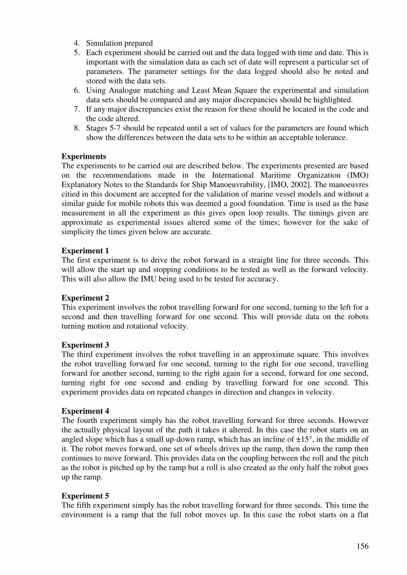
156
4. Simulation prepared 5. Each experiment should be carried out and the data logged with time and date. This is
important with the simulation data as each set of date will represent a particular set of parameters. The parameter settings for the data logged should also be noted and stored with the data sets.
6. Using Analogue matching and Least Mean Square the experimental and simulation data sets should be compared and any major discrepancies should be highlighted.
7. If any major discrepancies exist the reason for these should be located in the code and the code altered.
8. Stages 5-7 should be repeated until a set of values for the parameters are found which show the differences between the data sets to be within an acceptable tolerance.
Experiments
The experiments to be carried out are described below. The experiments presented are based on the recommendations made in the International Maritime Organization (IMO) Explanatory Notes to the Standards for Ship Manoeuvrability, [IMO, 2002]. The manoeuvres citied in this document are accepted for the validation of marine vessel models and without a similar guide for mobile robots this was deemed a good foundation. Time is used as the base measurement in all the experiment as this gives open loop results. The timings given are approximate as experimental issues altered some of the times; however for the sake of simplicity the times given below are accurate. Experiment 1
The first experiment is to drive the robot forward in a straight line for three seconds. This will allow the start up and stopping conditions to be tested as well as the forward velocity. This will also allow the IMU being used to be tested for accuracy. Experiment 2
This experiment involves the robot travelling forward for one second, turning to the left for a second and then travelling forward for one second. This will provide data on the robots turning motion and rotational velocity. Experiment 3
The third experiment involves the robot travelling in an approximate square. This involves the robot travelling forward for one second, turning to the right for one second, travelling forward for another second, turning to the right again for a second, forward for one second, turning right for one second and ending by travelling forward for one second. This experiment provides data on repeated changes in direction and changes in velocity. Experiment 4
The fourth experiment simply has the robot travelling forward for three seconds. However the actually physical layout of the path it takes it altered. In this case the robot starts on an angled slope which has a small up-down ramp, which has an incline of ±15°, in the middle of it. The robot moves forward, one set of wheels drives up the ramp, then down the ramp then continues to move forward. This provides data on the coupling between the roll and the pitch as the robot is pitched up by the ramp but a roll is also created as the only half the robot goes up the ramp. Experiment 5
The fifth experiment simply has the robot travelling forward for three seconds. This time the environment is a ramp that the full robot moves up. In this case the robot starts on a flat
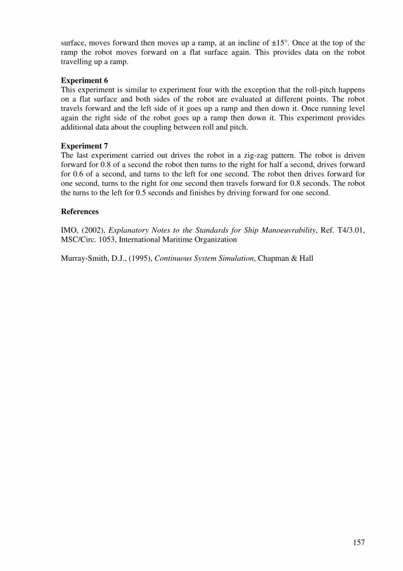
157
surface, moves forward then moves up a ramp, at an incline of ±15°. Once at the top of the ramp the robot moves forward on a flat surface again. This provides data on the robot travelling up a ramp. Experiment 6
This experiment is similar to experiment four with the exception that the roll-pitch happens on a flat surface and both sides of the robot are evaluated at different points. The robot travels forward and the left side of it goes up a ramp and then down it. Once running level again the right side of the robot goes up a ramp then down it. This experiment provides additional data about the coupling between roll and pitch. Experiment 7
The last experiment carried out drives the robot in a zig-zag pattern. The robot is driven forward for 0.8 of a second the robot then turns to the right for half a second, drives forward for 0.6 of a second, and turns to the left for one second. The robot then drives forward for one second, turns to the right for one second then travels forward for 0.8 seconds. The robot the turns to the left for 0.5 seconds and finishes by driving forward for one second. References
IMO, (2002), Explanatory Notes to the Standards for Ship Manoeuvrability, Ref. T4/3.01, MSC/Circ. 1053, International Maritime Organization Murray-Smith, D.J., (1995), Continuous System Simulation, Chapman & Hall
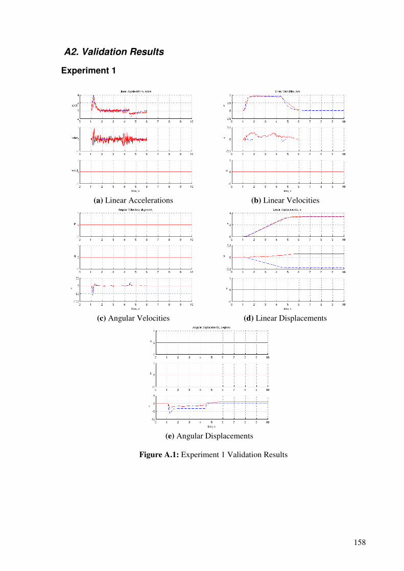
158
A2. Validation Results
Experiment 1
(a) Linear Accelerations (b) Linear Velocities
(c) Angular Velocities (d) Linear Displacements
(e) Angular Displacements
Figure A.1: Experiment 1 Validation Results
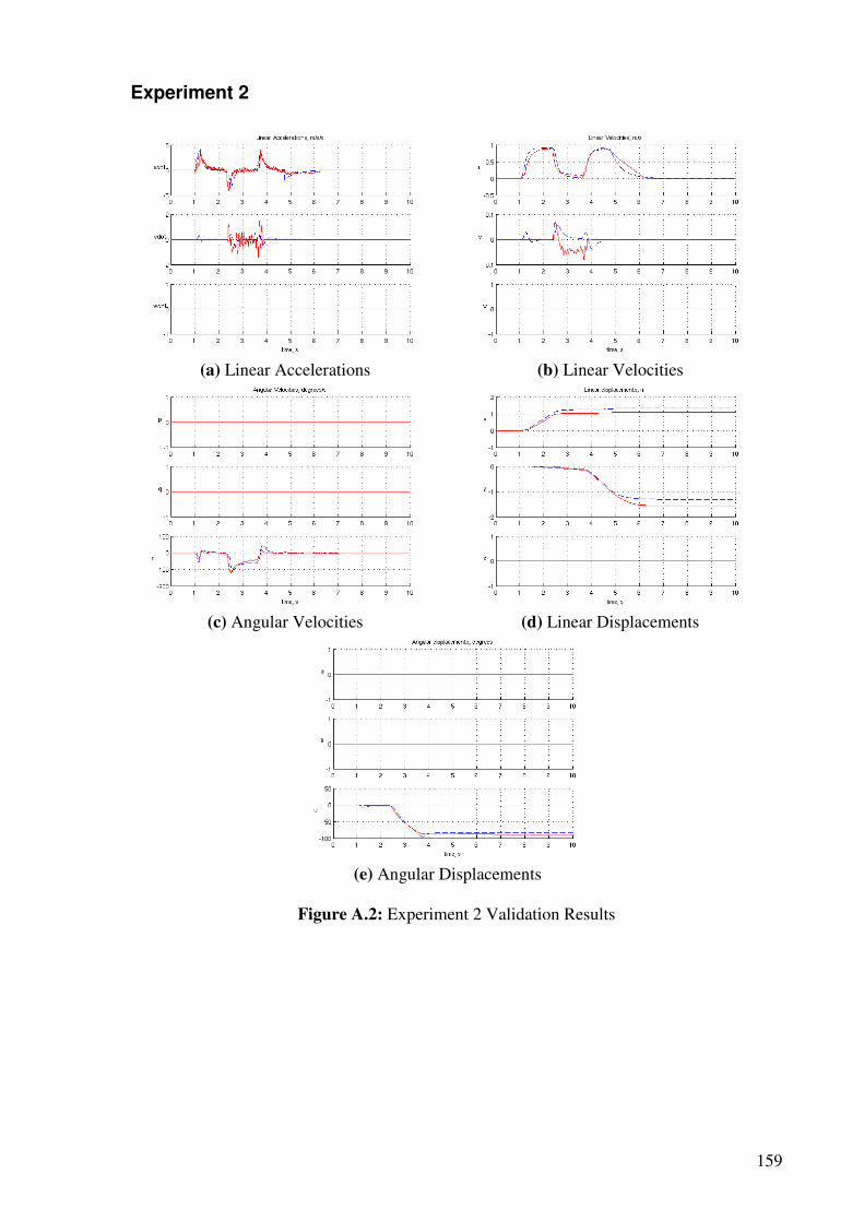
159
Experiment 2
(a) Linear Accelerations (b) Linear Velocities
(c) Angular Velocities (d) Linear Displacements
(e) Angular Displacements
Figure A.2: Experiment 2 Validation Results
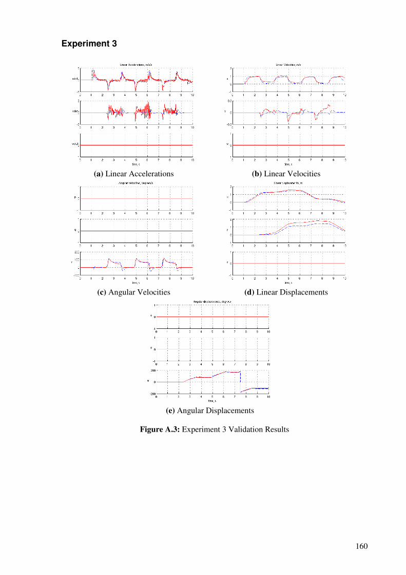
160
Experiment 3
(a) Linear Accelerations (b) Linear Velocities
(c) Angular Velocities (d) Linear Displacements
(e) Angular Displacements
Figure A.3: Experiment 3 Validation Results
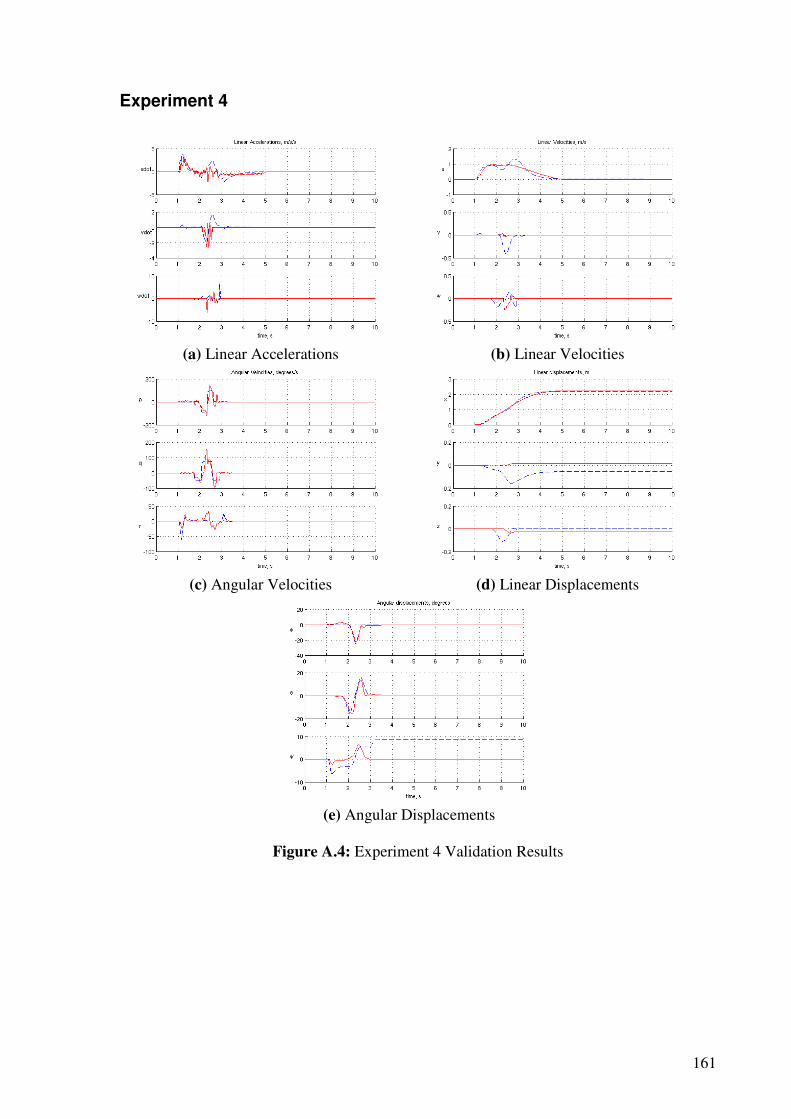
161
Experiment 4
(a) Linear Accelerations (b) Linear Velocities
(c) Angular Velocities (d) Linear Displacements
(e) Angular Displacements
Figure A.4: Experiment 4 Validation Results
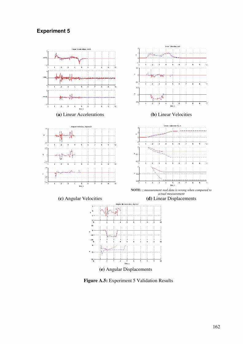
162
Experiment 5
(a) Linear Accelerations (b) Linear Velocities
NOTE: z measurement real data is wrong when compared to
actual measurement
(c) Angular Velocities (d) Linear Displacements
(e) Angular Displacements
Figure A.5: Experiment 5 Validation Results
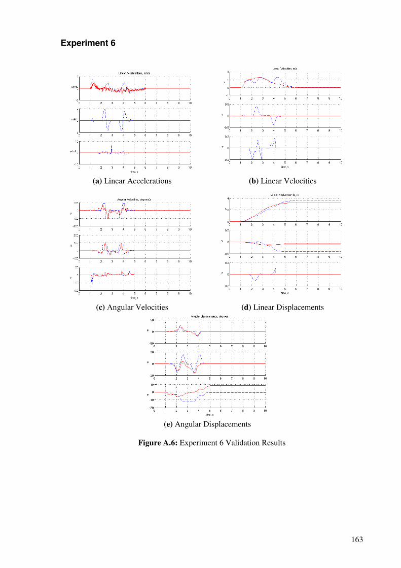
163
Experiment 6
(a) Linear Accelerations (b) Linear Velocities
(c) Angular Velocities (d) Linear Displacements
(e) Angular Displacements
Figure A.6: Experiment 6 Validation Results
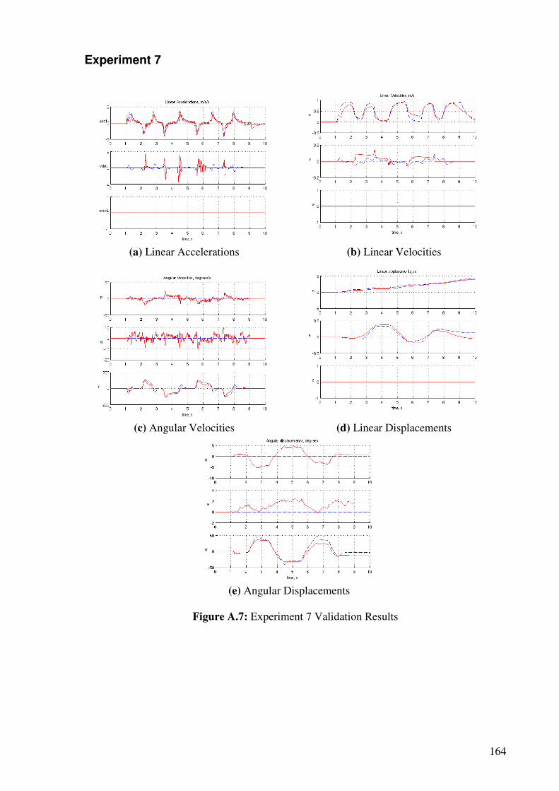
164
Experiment 7
(a) Linear Accelerations (b) Linear Velocities
(c) Angular Velocities (d) Linear Displacements
(e) Angular Displacements
Figure A.7: Experiment 7 Validation Results
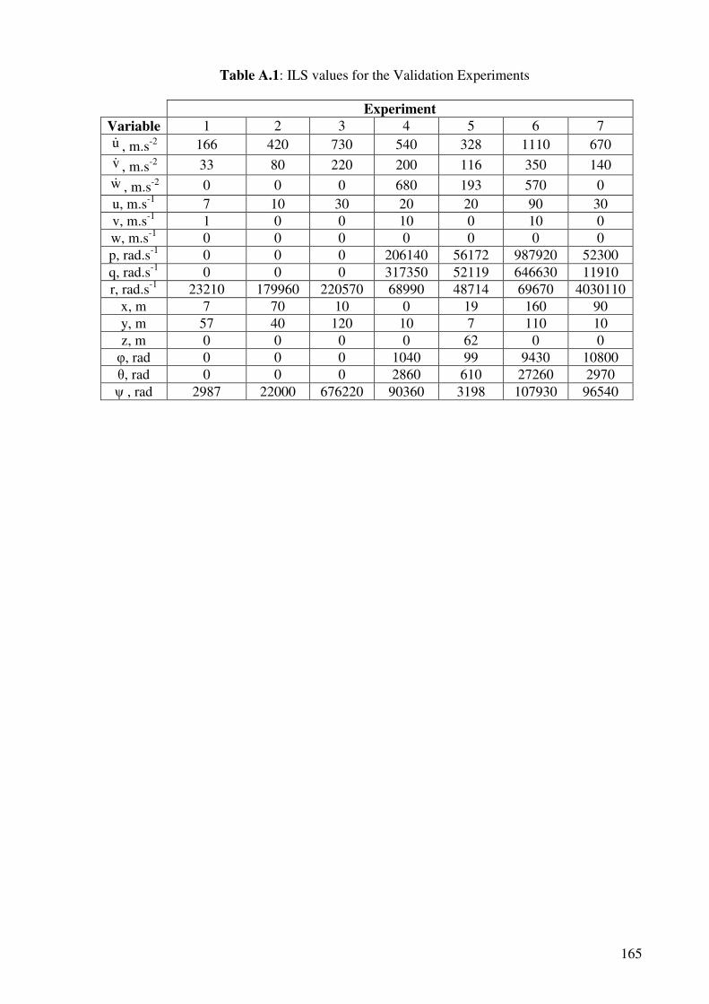
165
Table A.1: ILS values for the Validation Experiments
Experiment
Variable 1 2 3 4 5 6 7 u& , m.s-2 166 420 730 540 328 1110 670 v& , m.s-2 33 80 220 200 116 350 140 w& , m.s-2 0 0 0 680 193 570 0 u, m.s-1 7 10 30 20 20 90 30 v, m.s-1 1 0 0 10 0 10 0 w, m.s-1 0 0 0 0 0 0 0 p, rad.s-1 0 0 0 206140 56172 987920 52300 q, rad.s-1 0 0 0 317350 52119 646630 11910 r, rad.s-1 23210 179960 220570 68990 48714 69670 4030110
x, m 7 70 10 0 19 160 90 y, m 57 40 120 10 7 110 10 z, m 0 0 0 0 62 0 0 φ, rad 0 0 0 1040 99 9430 10800 θ, rad 0 0 0 2860 610 27260 2970 ψ , rad 2987 22000 676220 90360 3198 107930 96540
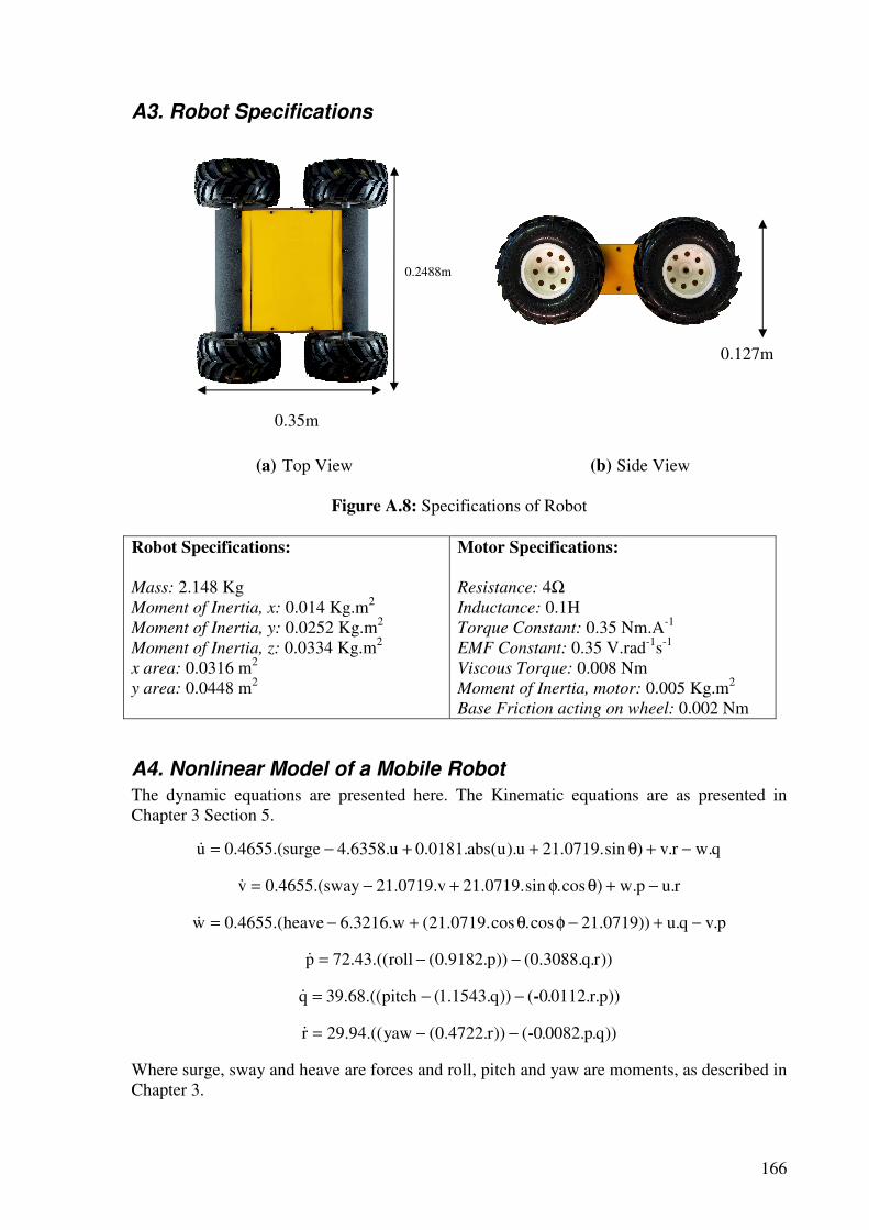
166
A3. Robot Specifications
(a) Top View (b) Side View
Figure A.8: Specifications of Robot Robot Specifications:
Mass: 2.148 Kg Moment of Inertia, x: 0.014 Kg.m2
Moment of Inertia, y: 0.0252 Kg.m2
Moment of Inertia, z: 0.0334 Kg.m2
x area: 0.0316 m2 y area: 0.0448 m2
Motor Specifications:
Resistance: 4Ω Inductance: 0.1H Torque Constant: 0.35 Nm.A-1
EMF Constant: 0.35 V.rad-1s-1 Viscous Torque: 0.008 Nm Moment of Inertia, motor: 0.005 Kg.m2
Base Friction acting on wheel: 0.002 Nm
A4. Nonlinear Model of a Mobile Robot
The dynamic equations are presented here. The Kinematic equations are as presented in Chapter 3 Section 5.
q.wr.v)sin.0719.21u).u(abs.0181.0u.6358.4surge.(4655.0u −+θ++−=&
r.up.w)cos.sin.0719.21v.0719.21sway.(4655.0v −+θφ+−=&
p.vq.u))0719.21cos.cos.0719.21(w.3216.6heave.(4655.0w −+−φθ+−=&
))r.q.3088.0())p.9182.0(roll.((43.72p −−=&
))p.r.0112.0())q.1543.1(pitch.((68.39q -−−=&
))q.p.0082.0())r.4722.0(yaw.((94.29r -−−=&
Where surge, sway and heave are forces and roll, pitch and yaw are moments, as described in Chapter 3.
0.127m
0.2488m
0.35m
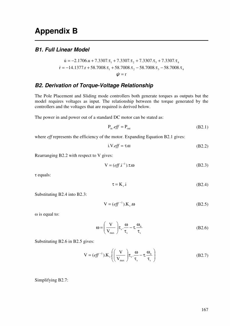
167
Appendix B
B1. Full Linear Model
4321 .3307.7.3307.7.3307.7.3307.7u.1706.2u τ+τ+τ+τ+−=&
4321 .7008.58.7008.58.7008.58.7008.58r.1377.14r τ−τ−τ+τ+−=&
r=ψ&
B2. Derivation of Torque-Voltage Relationship
The Pole Placement and Sliding mode controllers both generate torques as outputs but the model requires voltages as input. The relationship between the torque generated by the controllers and the voltages that are required is derived below. The power in and power out of a standard DC motor can be stated as:
outin P.P =eff (B2.1)
where eff represents the efficiency of the motor. Expanding Equation B2.1 gives:
ωτ= ..V.i eff (B2.2)
Rearranging B2.2 with respect to V gives:
ωτ= − .).i.(V 1eff (B2.3)
τ equals:
i.K t=τ (B2.4)
Substituting B2.4 into B2.3:
ω= − .K).(V t1
eff (B2.5)
ω is equal to:
s
n
ss
max
...V
V
τ
ωτ−
τ
ωτ
=ω (B2.6)
Substituting B2.6 in B2.5 gives:
τ
ωτ−
τ
ωτ
= −
s
n
ss
maxt
1 ...V
V.K).(V eff (B2.7)
Simplifying B2.7:
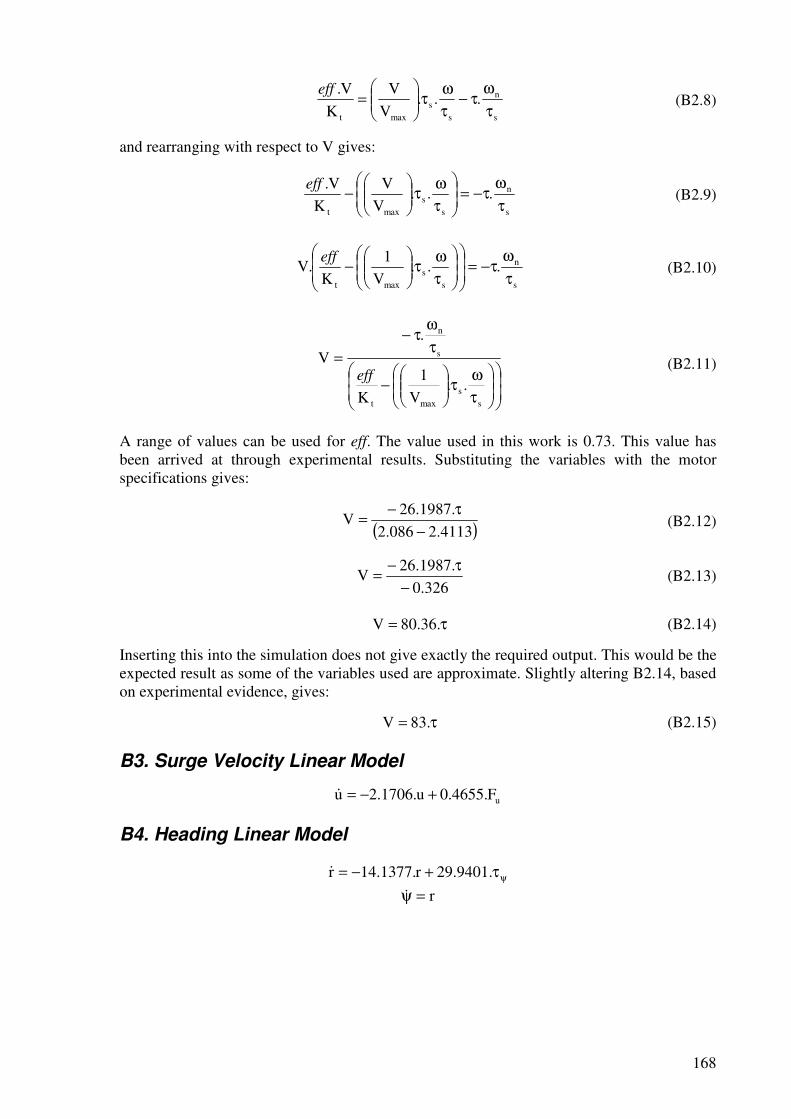
168
s
n
ss
maxt
...V
V
K
V.
τ
ωτ−
τ
ωτ
=
eff (B2.8)
and rearranging with respect to V gives:
s
n
ss
maxt
...V
V
K
V.
τ
ωτ−=
τ
ωτ
−
eff (B2.9)
s
n
ss
maxt
...V
1
K.V
τ
ωτ−=
τ
ωτ
−
eff (B2.10)
τ
ωτ
−
τ
ωτ−
=
ss
maxt
s
n
..V
1
K
.
Veff
(B2.11)
A range of values can be used for eff. The value used in this work is 0.73. This value has been arrived at through experimental results. Substituting the variables with the motor specifications gives:
( )4113.2086.2
.1987.26V
−
τ−= (B2.12)
326.0.1987.26
V−
τ−= (B2.13)
τ= .36.80V (B2.14)
Inserting this into the simulation does not give exactly the required output. This would be the expected result as some of the variables used are approximate. Slightly altering B2.14, based on experimental evidence, gives:
τ= .83V (B2.15)
B3. Surge Velocity Linear Model
uF.4655.0u.1706.2u +−=&
B4. Heading Linear Model
ψτ+−= .9401.29r.1377.14r&
r=ψ&
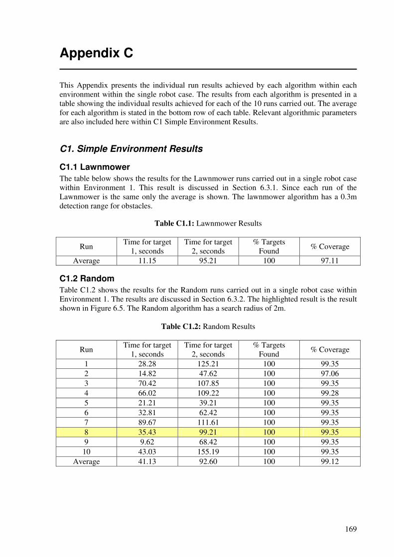
169
Appendix C
This Appendix presents the individual run results achieved by each algorithm within each environment within the single robot case. The results from each algorithm is presented in a table showing the individual results achieved for each of the 10 runs carried out. The average for each algorithm is stated in the bottom row of each table. Relevant algorithmic parameters are also included here within C1 Simple Environment Results.
C1. Simple Environment Results
C1.1 Lawnmower
The table below shows the results for the Lawnmower runs carried out in a single robot case within Environment 1. This result is discussed in Section 6.3.1. Since each run of the Lawnmower is the same only the average is shown. The lawnmower algorithm has a 0.3m detection range for obstacles.
Table C1.1: Lawnmower Results
Run Time for target
1, seconds Time for target
2, seconds % Targets
Found % Coverage
Average 11.15 95.21 100 97.11
C1.2 Random
Table C1.2 shows the results for the Random runs carried out in a single robot case within Environment 1. The results are discussed in Section 6.3.2. The highlighted result is the result shown in Figure 6.5. The Random algorithm has a search radius of 2m.
Table C1.2: Random Results
Run Time for target
1, seconds Time for target
2, seconds % Targets
Found % Coverage
1 28.28 125.21 100 99.35 2 14.82 47.62 100 97.06 3 70.42 107.85 100 99.35 4 66.02 109.22 100 99.28 5 21.21 39.21 100 99.35 6 32.81 62.42 100 99.35 7 89.67 111.61 100 99.35 8 35.43 99.21 100 99.35 9 9.62 68.42 100 99.35
10 43.03 155.19 100 99.35 Average 41.13 92.60 100 99.12
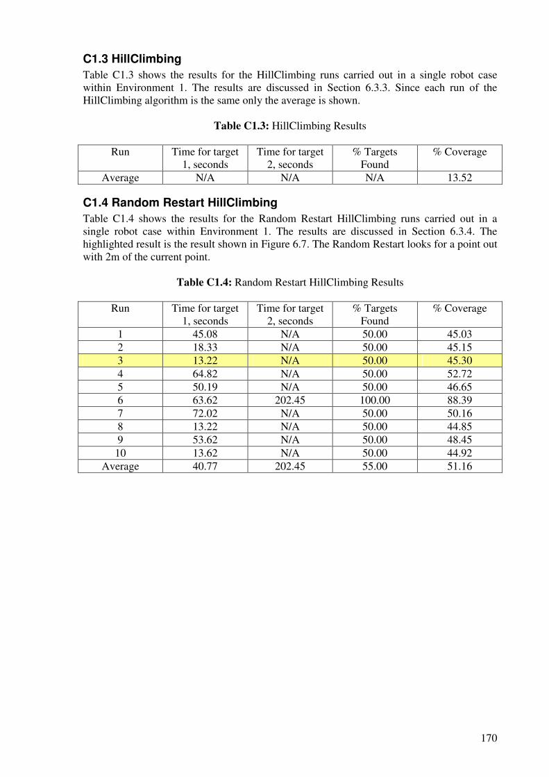
170
C1.3 HillClimbing
Table C1.3 shows the results for the HillClimbing runs carried out in a single robot case within Environment 1. The results are discussed in Section 6.3.3. Since each run of the HillClimbing algorithm is the same only the average is shown.
Table C1.3: HillClimbing Results
Run Time for target
1, seconds Time for target
2, seconds % Targets
Found % Coverage
Average N/A N/A N/A 13.52
C1.4 Random Restart HillClimbing
Table C1.4 shows the results for the Random Restart HillClimbing runs carried out in a single robot case within Environment 1. The results are discussed in Section 6.3.4. The highlighted result is the result shown in Figure 6.7. The Random Restart looks for a point out with 2m of the current point.
Table C1.4: Random Restart HillClimbing Results
Run Time for target
1, seconds Time for target
2, seconds % Targets
Found % Coverage
1 45.08 N/A 50.00 45.03 2 18.33 N/A 50.00 45.15 3 13.22 N/A 50.00 45.30 4 64.82 N/A 50.00 52.72 5 50.19 N/A 50.00 46.65 6 63.62 202.45 100.00 88.39 7 72.02 N/A 50.00 50.16 8 13.22 N/A 50.00 44.85 9 53.62 N/A 50.00 48.45
10 13.62 N/A 50.00 44.92 Average 40.77 202.45 55.00 51.16
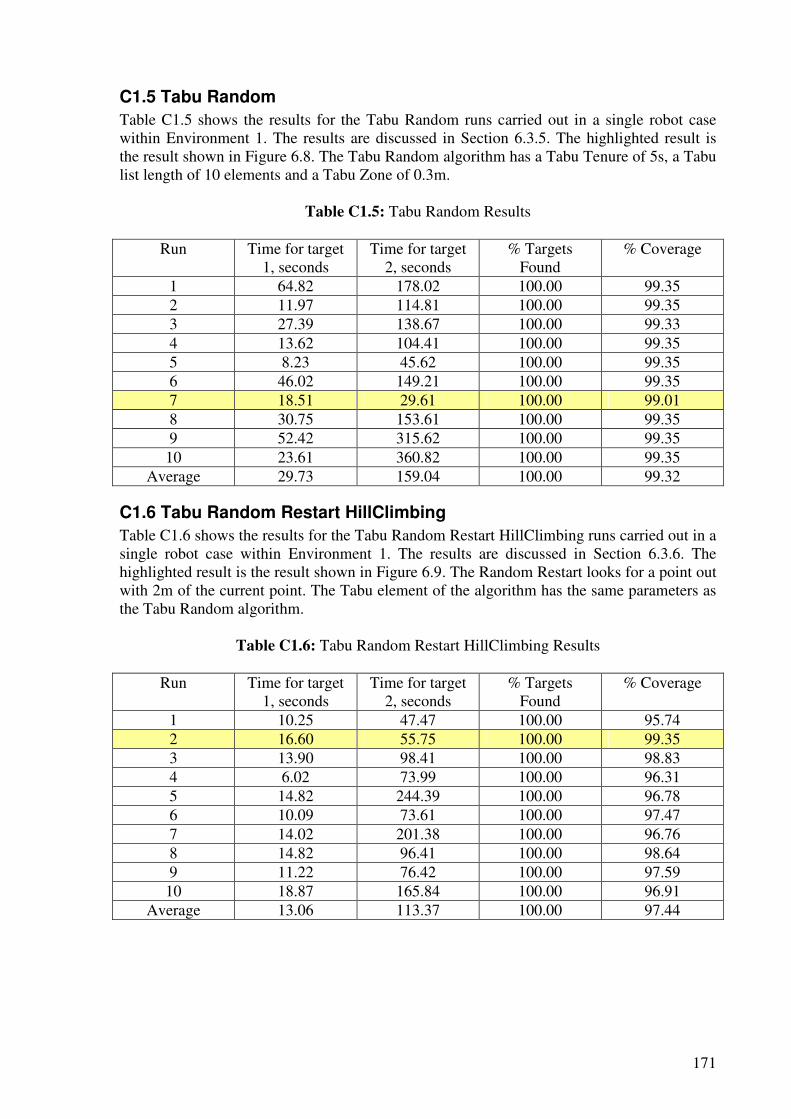
171
C1.5 Tabu Random
Table C1.5 shows the results for the Tabu Random runs carried out in a single robot case within Environment 1. The results are discussed in Section 6.3.5. The highlighted result is the result shown in Figure 6.8. The Tabu Random algorithm has a Tabu Tenure of 5s, a Tabu list length of 10 elements and a Tabu Zone of 0.3m.
Table C1.5: Tabu Random Results
Run Time for target 1, seconds
Time for target 2, seconds
% Targets Found
% Coverage
1 64.82 178.02 100.00 99.35 2 11.97 114.81 100.00 99.35 3 27.39 138.67 100.00 99.33 4 13.62 104.41 100.00 99.35 5 8.23 45.62 100.00 99.35 6 46.02 149.21 100.00 99.35 7 18.51 29.61 100.00 99.01 8 30.75 153.61 100.00 99.35 9 52.42 315.62 100.00 99.35
10 23.61 360.82 100.00 99.35 Average 29.73 159.04 100.00 99.32
C1.6 Tabu Random Restart HillClimbing
Table C1.6 shows the results for the Tabu Random Restart HillClimbing runs carried out in a single robot case within Environment 1. The results are discussed in Section 6.3.6. The highlighted result is the result shown in Figure 6.9. The Random Restart looks for a point out with 2m of the current point. The Tabu element of the algorithm has the same parameters as the Tabu Random algorithm.
Table C1.6: Tabu Random Restart HillClimbing Results
Run Time for target
1, seconds Time for target
2, seconds % Targets
Found % Coverage
1 10.25 47.47 100.00 95.74 2 16.60 55.75 100.00 99.35 3 13.90 98.41 100.00 98.83 4 6.02 73.99 100.00 96.31 5 14.82 244.39 100.00 96.78 6 10.09 73.61 100.00 97.47 7 14.02 201.38 100.00 96.76 8 14.82 96.41 100.00 98.64 9 11.22 76.42 100.00 97.59
10 18.87 165.84 100.00 96.91 Average 13.06 113.37 100.00 97.44
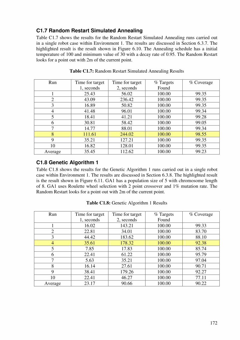
172
C1.7 Random Restart Simulated Annealing
Table C1.7 shows the results for the Random Restart Simulated Annealing runs carried out in a single robot case within Environment 1. The results are discussed in Section 6.3.7. The highlighted result is the result shown in Figure 6.10. The Annealing schedule has a initial temperature of 100 and minimum value of 30 with a decay rate of 0.95. The Random Restart looks for a point out with 2m of the current point.
Table C1.7: Random Restart Simulated Annealing Results
Run Time for target
1, seconds Time for target
2, seconds % Targets
Found % Coverage
1 25.43 56.02 100.00 99.35 2 43.09 236.42 100.00 99.35 3 16.89 50.82 100.00 99.35 4 41.48 96.01 100.00 99.34 5 18.41 41.21 100.00 99.28 6 30.81 58.42 100.00 99.05 7 14.77 88.01 100.00 99.34 8 111.61 244.02 100.00 98.55 9 35.21 127.21 100.00 99.35
10 16.82 128.01 100.00 99.35 Average 35.45 112.62 100.00 99.23
C1.8 Genetic Algorithm 1
Table C1.8 shows the results for the Genetic Algorithm 1 runs carried out in a single robot case within Environment 1. The results are discussed in Section 6.3.8. The highlighted result is the result shown in Figure 6.11. GA1 has a population size of 5 with chromosome length of 8. GA1 uses Roulette wheel selection with 2 point crossover and 1% mutation rate. The Random Restart looks for a point out with 2m of the current point.
Table C1.8: Genetic Algorithm 1 Results
Run Time for target 1, seconds
Time for target 2, seconds
% Targets Found
% Coverage
1 16.02 143.21 100.00 99.33 2 22.81 34.01 100.00 83.70 3 44.42 183.62 100.00 88.10 4 35.61 178.32 100.00 92.38 5 7.85 17.83 100.00 85.74 6 22.41 61.22 100.00 95.79 7 5.63 35.21 100.00 97.04 8 16.14 27.61 100.00 90.71 9 38.41 179.26 100.00 92.27
10 22.41 46.27 100.00 77.11 Average 23.17 90.66 100.00 90.22
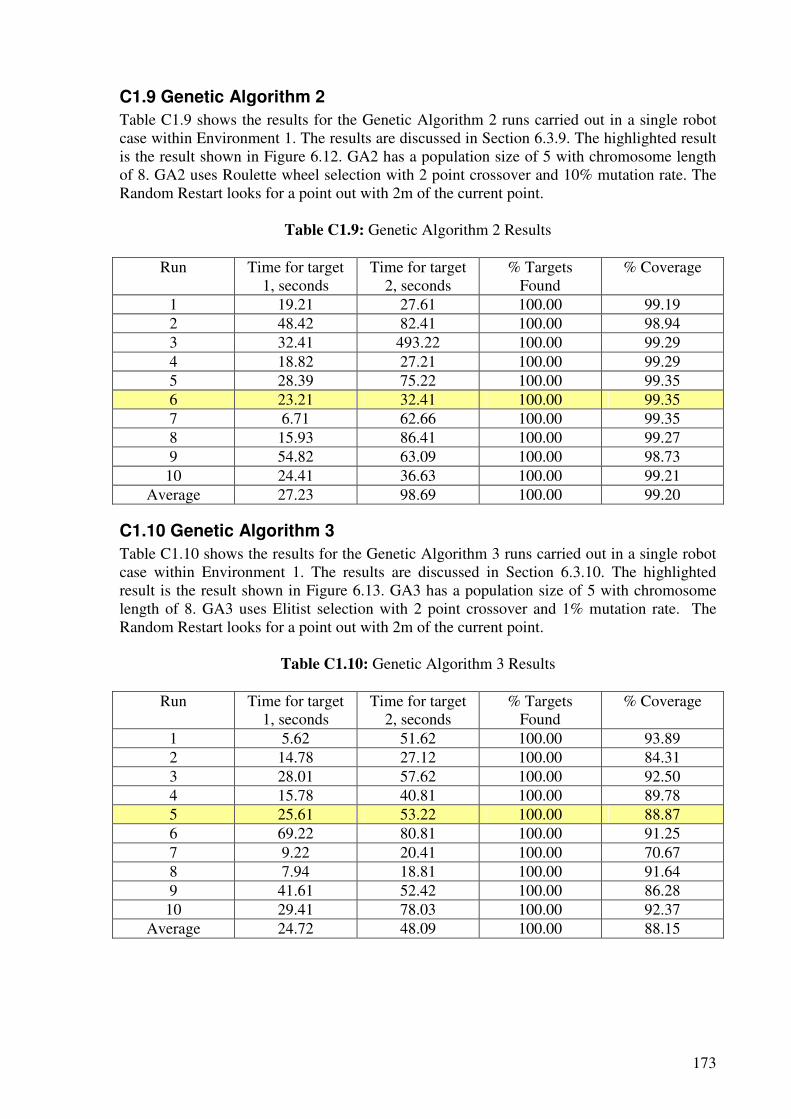
173
C1.9 Genetic Algorithm 2
Table C1.9 shows the results for the Genetic Algorithm 2 runs carried out in a single robot case within Environment 1. The results are discussed in Section 6.3.9. The highlighted result is the result shown in Figure 6.12. GA2 has a population size of 5 with chromosome length of 8. GA2 uses Roulette wheel selection with 2 point crossover and 10% mutation rate. The Random Restart looks for a point out with 2m of the current point.
Table C1.9: Genetic Algorithm 2 Results
Run Time for target
1, seconds Time for target
2, seconds % Targets
Found % Coverage
1 19.21 27.61 100.00 99.19 2 48.42 82.41 100.00 98.94 3 32.41 493.22 100.00 99.29 4 18.82 27.21 100.00 99.29 5 28.39 75.22 100.00 99.35 6 23.21 32.41 100.00 99.35 7 6.71 62.66 100.00 99.35 8 15.93 86.41 100.00 99.27 9 54.82 63.09 100.00 98.73
10 24.41 36.63 100.00 99.21 Average 27.23 98.69 100.00 99.20
C1.10 Genetic Algorithm 3
Table C1.10 shows the results for the Genetic Algorithm 3 runs carried out in a single robot case within Environment 1. The results are discussed in Section 6.3.10. The highlighted result is the result shown in Figure 6.13. GA3 has a population size of 5 with chromosome length of 8. GA3 uses Elitist selection with 2 point crossover and 1% mutation rate. The Random Restart looks for a point out with 2m of the current point.
Table C1.10: Genetic Algorithm 3 Results
Run Time for target 1, seconds
Time for target 2, seconds
% Targets Found
% Coverage
1 5.62 51.62 100.00 93.89 2 14.78 27.12 100.00 84.31 3 28.01 57.62 100.00 92.50 4 15.78 40.81 100.00 89.78 5 25.61 53.22 100.00 88.87 6 69.22 80.81 100.00 91.25 7 9.22 20.41 100.00 70.67 8 7.94 18.81 100.00 91.64 9 41.61 52.42 100.00 86.28
10 29.41 78.03 100.00 92.37 Average 24.72 48.09 100.00 88.15
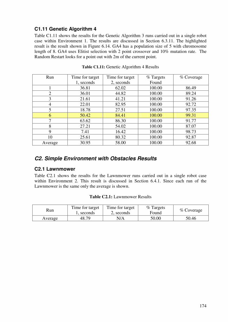
174
C1.11 Genetic Algorithm 4
Table C1.11 shows the results for the Genetic Algorithm 3 runs carried out in a single robot case within Environment 1. The results are discussed in Section 6.3.11. The highlighted result is the result shown in Figure 6.14. GA4 has a population size of 5 with chromosome length of 8. GA4 uses Elitist selection with 2 point crossover and 10% mutation rate. The Random Restart looks for a point out with 2m of the current point.
Table C1.11: Genetic Algorithm 4 Results
Run Time for target
1, seconds Time for target
2, seconds % Targets
Found % Coverage
1 36.81 62.02 100.00 86.49 2 36.01 44.82 100.00 89.24 3 21.61 41.21 100.00 91.26 4 22.01 82.95 100.00 92.72 5 18.78 27.51 100.00 97.35 6 50.42 84.41 100.00 99.31 7 63.62 86.30 100.00 91.77 8 27.21 54.02 100.00 87.07 9 7.41 16.42 100.00 98.73
10 25.61 80.32 100.00 92.87 Average 30.95 58.00 100.00 92.68
C2. Simple Environment with Obstacles Results
C2.1 Lawnmower
Table C2.1 shows the results for the Lawnmower runs carried out in a single robot case within Environment 2. This result is discussed in Section 6.4.1. Since each run of the Lawnmower is the same only the average is shown.
Table C2.1: Lawnmower Results
Run Time for target
1, seconds Time for target
2, seconds % Targets
Found % Coverage
Average 48.79 N/A 50.00 50.46
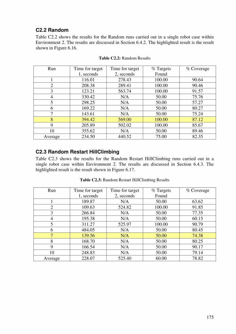
175
C2.2 Random
Table C2.2 shows the results for the Random runs carried out in a single robot case within Environment 2. The results are discussed in Section 6.4.2. The highlighted result is the result shown in Figure 6.16.
Table C2.2: Random Results
Run Time for target
1, seconds Time for target
2, seconds % Targets
Found % Coverage
1 116.01 278.43 100.00 90.64 2 208.38 289.41 100.00 90.46 3 123.21 563.74 100.00 91.57 4 330.42 N/A 50.00 75.76 5 298.25 N/A 50.00 57.27 6 169.22 N/A 50.00 80.27 7 143.61 N/A 50.00 75.24 8 394.42 569.00 100.00 87.12 9 205.89 502.02 100.00 85.67
10 355.62 N/A 50.00 89.46 Average 234.50 440.52 75.00 82.35
C2.3 Random Restart HillClimbing
Table C2.3 shows the results for the Random Restart HillClimbing runs carried out in a single robot case within Environment 2. The results are discussed in Section 6.4.3. The highlighted result is the result shown in Figure 6.17.
Table C2.3: Random Restart HillClimbing Results
Run Time for target 1, seconds
Time for target 2, seconds
% Targets Found
% Coverage
1 189.87 N/A 50.00 63.62 2 109.63 524.82 100.00 91.85 3 266.84 N/A 50.00 77.35 4 195.38 N/A 50.00 60.15 5 311.27 525.97 100.00 90.79 6 484.05 N/A 50.00 80.45 7 139.56 N/A 50.00 74.38 8 168.70 N/A 50.00 80.25 9 166.54 N/A 50.00 90.17
10 248.83 N/A 50.00 79.14 Average 228.07 525.40 60.00 78.82
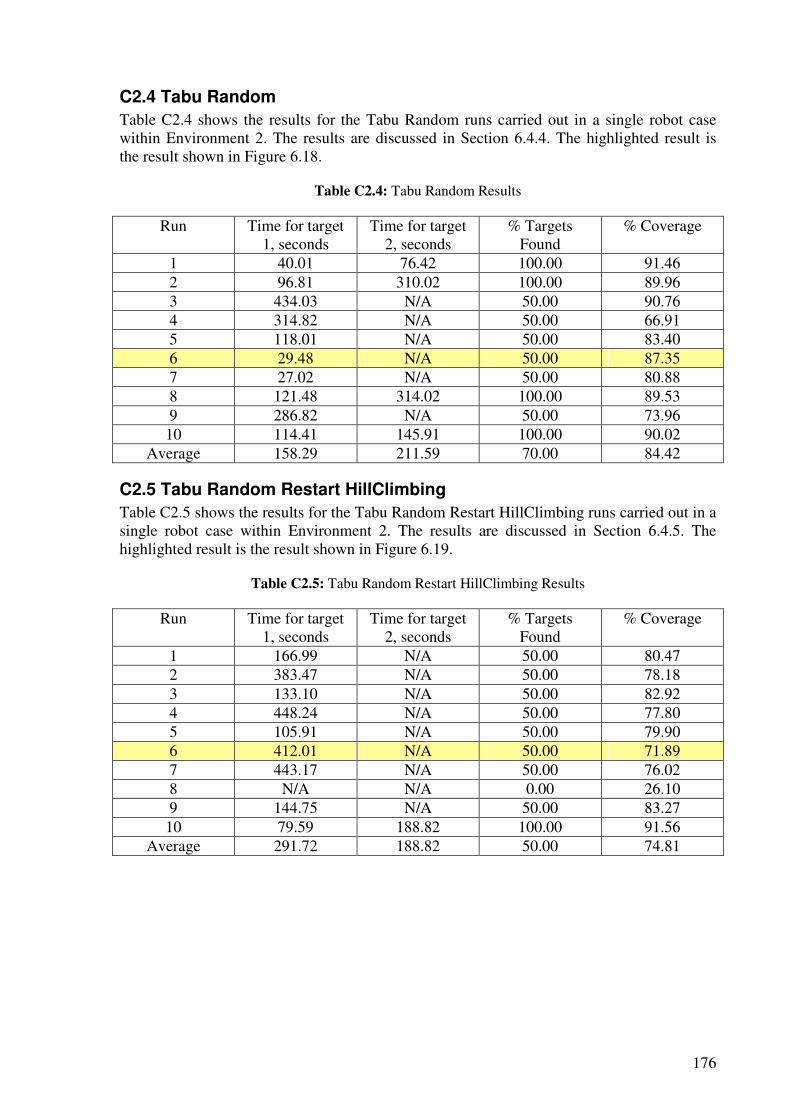
176
C2.4 Tabu Random
Table C2.4 shows the results for the Tabu Random runs carried out in a single robot case within Environment 2. The results are discussed in Section 6.4.4. The highlighted result is the result shown in Figure 6.18.
Table C2.4: Tabu Random Results
Run Time for target 1, seconds
Time for target 2, seconds
% Targets Found
% Coverage
1 40.01 76.42 100.00 91.46 2 96.81 310.02 100.00 89.96 3 434.03 N/A 50.00 90.76 4 314.82 N/A 50.00 66.91 5 118.01 N/A 50.00 83.40 6 29.48 N/A 50.00 87.35 7 27.02 N/A 50.00 80.88 8 121.48 314.02 100.00 89.53 9 286.82 N/A 50.00 73.96
10 114.41 145.91 100.00 90.02 Average 158.29 211.59 70.00 84.42
C2.5 Tabu Random Restart HillClimbing
Table C2.5 shows the results for the Tabu Random Restart HillClimbing runs carried out in a single robot case within Environment 2. The results are discussed in Section 6.4.5. The highlighted result is the result shown in Figure 6.19.
Table C2.5: Tabu Random Restart HillClimbing Results
Run Time for target
1, seconds Time for target
2, seconds % Targets
Found % Coverage
1 166.99 N/A 50.00 80.47 2 383.47 N/A 50.00 78.18 3 133.10 N/A 50.00 82.92 4 448.24 N/A 50.00 77.80 5 105.91 N/A 50.00 79.90 6 412.01 N/A 50.00 71.89 7 443.17 N/A 50.00 76.02 8 N/A N/A 0.00 26.10 9 144.75 N/A 50.00 83.27
10 79.59 188.82 100.00 91.56 Average 291.72 188.82 50.00 74.81
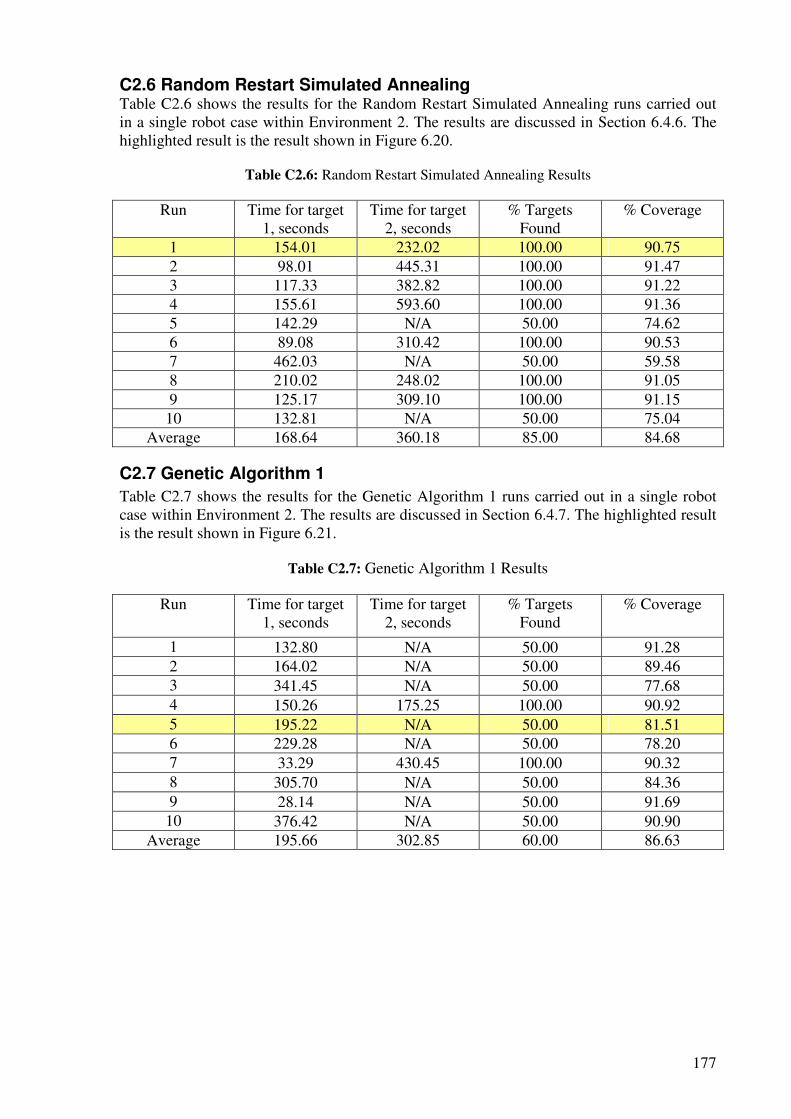
177
C2.6 Random Restart Simulated Annealing Table C2.6 shows the results for the Random Restart Simulated Annealing runs carried out in a single robot case within Environment 2. The results are discussed in Section 6.4.6. The highlighted result is the result shown in Figure 6.20.
Table C2.6: Random Restart Simulated Annealing Results
Run Time for target
1, seconds Time for target
2, seconds % Targets
Found % Coverage
1 154.01 232.02 100.00 90.75 2 98.01 445.31 100.00 91.47 3 117.33 382.82 100.00 91.22 4 155.61 593.60 100.00 91.36 5 142.29 N/A 50.00 74.62 6 89.08 310.42 100.00 90.53 7 462.03 N/A 50.00 59.58 8 210.02 248.02 100.00 91.05 9 125.17 309.10 100.00 91.15
10 132.81 N/A 50.00 75.04 Average 168.64 360.18 85.00 84.68
C2.7 Genetic Algorithm 1
Table C2.7 shows the results for the Genetic Algorithm 1 runs carried out in a single robot case within Environment 2. The results are discussed in Section 6.4.7. The highlighted result is the result shown in Figure 6.21.
Table C2.7: Genetic Algorithm 1 Results
Run Time for target
1, seconds Time for target
2, seconds % Targets
Found % Coverage
1 132.80 N/A 50.00 91.28 2 164.02 N/A 50.00 89.46 3 341.45 N/A 50.00 77.68 4 150.26 175.25 100.00 90.92 5 195.22 N/A 50.00 81.51 6 229.28 N/A 50.00 78.20 7 33.29 430.45 100.00 90.32 8 305.70 N/A 50.00 84.36 9 28.14 N/A 50.00 91.69
10 376.42 N/A 50.00 90.90 Average 195.66 302.85 60.00 86.63
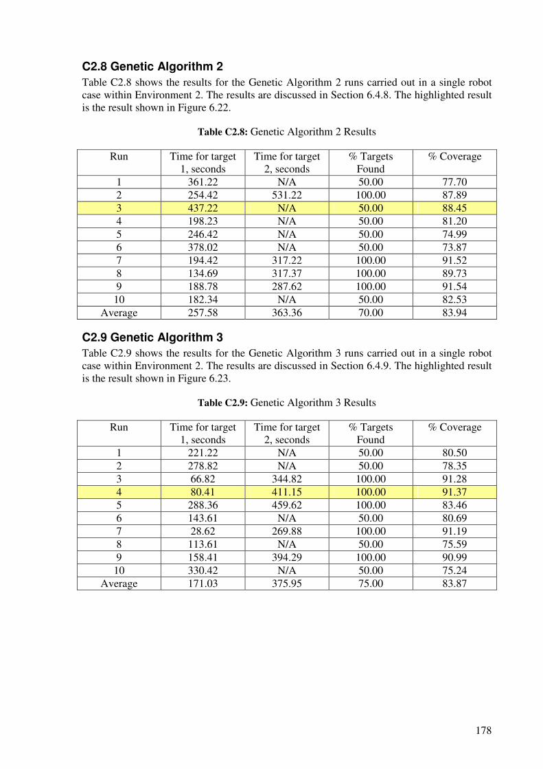
178
C2.8 Genetic Algorithm 2
Table C2.8 shows the results for the Genetic Algorithm 2 runs carried out in a single robot case within Environment 2. The results are discussed in Section 6.4.8. The highlighted result is the result shown in Figure 6.22.
Table C2.8: Genetic Algorithm 2 Results
Run Time for target
1, seconds Time for target
2, seconds % Targets
Found % Coverage
1 361.22 N/A 50.00 77.70 2 254.42 531.22 100.00 87.89 3 437.22 N/A 50.00 88.45 4 198.23 N/A 50.00 81.20 5 246.42 N/A 50.00 74.99 6 378.02 N/A 50.00 73.87 7 194.42 317.22 100.00 91.52 8 134.69 317.37 100.00 89.73 9 188.78 287.62 100.00 91.54
10 182.34 N/A 50.00 82.53 Average 257.58 363.36 70.00 83.94
C2.9 Genetic Algorithm 3
Table C2.9 shows the results for the Genetic Algorithm 3 runs carried out in a single robot case within Environment 2. The results are discussed in Section 6.4.9. The highlighted result is the result shown in Figure 6.23.
Table C2.9: Genetic Algorithm 3 Results
Run Time for target
1, seconds Time for target
2, seconds % Targets
Found % Coverage
1 221.22 N/A 50.00 80.50 2 278.82 N/A 50.00 78.35 3 66.82 344.82 100.00 91.28 4 80.41 411.15 100.00 91.37 5 288.36 459.62 100.00 83.46 6 143.61 N/A 50.00 80.69 7 28.62 269.88 100.00 91.19 8 113.61 N/A 50.00 75.59 9 158.41 394.29 100.00 90.99
10 330.42 N/A 50.00 75.24 Average 171.03 375.95 75.00 83.87
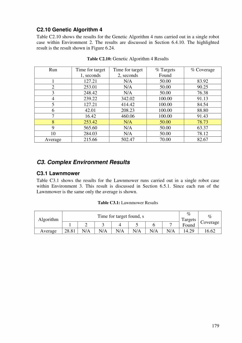
179
C2.10 Genetic Algorithm 4
Table C2.10 shows the results for the Genetic Algorithm 4 runs carried out in a single robot case within Environment 2. The results are discussed in Section 6.4.10. The highlighted result is the result shown in Figure 6.24.
Table C2.10: Genetic Algorithm 4 Results
Run Time for target
1, seconds Time for target
2, seconds % Targets
Found % Coverage
1 127.21 N/A 50.00 83.92 2 253.01 N/A 50.00 90.25 3 248.42 N/A 50.00 76.38 4 239.22 342.02 100.00 91.13 5 127.21 414.42 100.00 84.54 6 42.01 208.23 100.00 88.80 7 16.42 460.06 100.00 91.43 8 253.42 N/A 50.00 78.73 9 565.60 N/A 50.00 63.37
10 284.03 N/A 50.00 78.12 Average 215.66 502.47 70.00 82.67
C3. Complex Environment Results
C3.1 Lawnmower
Table C3.1 shows the results for the Lawnmower runs carried out in a single robot case within Environment 3. This result is discussed in Section 6.5.1. Since each run of the Lawnmower is the same only the average is shown.
Table C3.1: Lawnmower Results
Time for target found, s Algorithm
1 2 3 4 5 6 7
% Targets Found
% Coverage
Average 28.81 N/A N/A N/A N/A N/A N/A 14.29 16.62
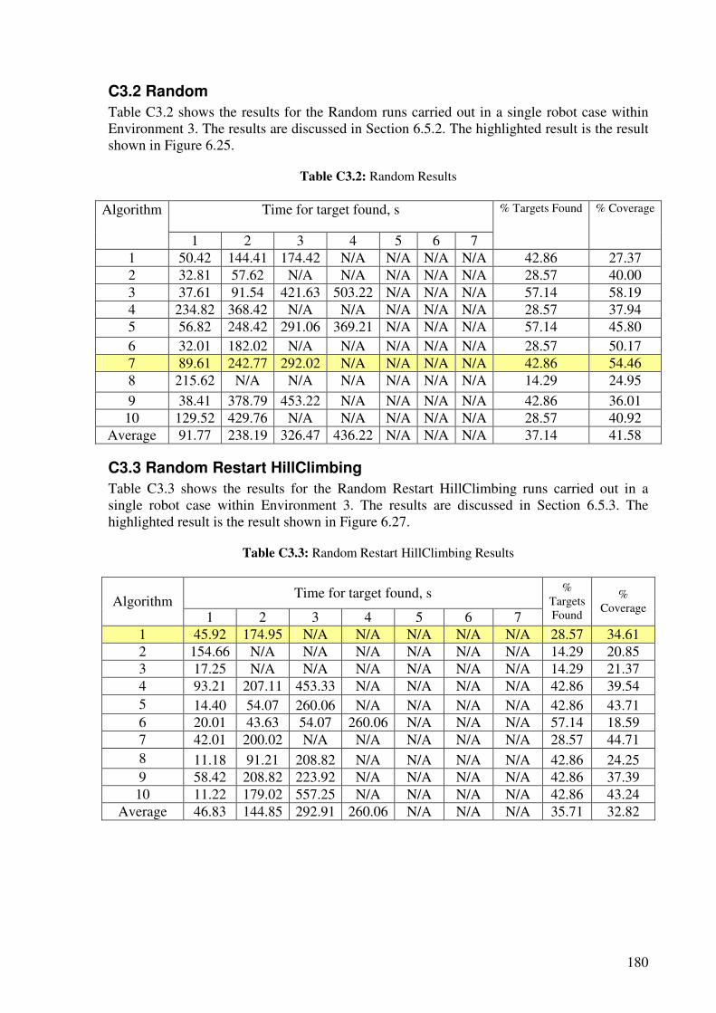
180
C3.2 Random
Table C3.2 shows the results for the Random runs carried out in a single robot case within Environment 3. The results are discussed in Section 6.5.2. The highlighted result is the result shown in Figure 6.25.
Table C3.2: Random Results
Time for target found, s Algorithm
1 2 3 4 5 6 7
% Targets Found % Coverage
1 50.42 144.41 174.42 N/A N/A N/A N/A 42.86 27.37 2 32.81 57.62 N/A N/A N/A N/A N/A 28.57 40.00 3 37.61 91.54 421.63 503.22 N/A N/A N/A 57.14 58.19 4 234.82 368.42 N/A N/A N/A N/A N/A 28.57 37.94 5 56.82 248.42 291.06 369.21 N/A N/A N/A 57.14 45.80 6 32.01 182.02 N/A N/A N/A N/A N/A 28.57 50.17 7 89.61 242.77 292.02 N/A N/A N/A N/A 42.86 54.46 8 215.62 N/A N/A N/A N/A N/A N/A 14.29 24.95 9 38.41 378.79 453.22 N/A N/A N/A N/A 42.86 36.01
10 129.52 429.76 N/A N/A N/A N/A N/A 28.57 40.92 Average 91.77 238.19 326.47 436.22 N/A N/A N/A 37.14 41.58
C3.3 Random Restart HillClimbing
Table C3.3 shows the results for the Random Restart HillClimbing runs carried out in a single robot case within Environment 3. The results are discussed in Section 6.5.3. The highlighted result is the result shown in Figure 6.27.
Table C3.3: Random Restart HillClimbing Results
Time for target found, s Algorithm
1 2 3 4 5 6 7
% Targets Found
% Coverage
1 45.92 174.95 N/A N/A N/A N/A N/A 28.57 34.61 2 154.66 N/A N/A N/A N/A N/A N/A 14.29 20.85 3 17.25 N/A N/A N/A N/A N/A N/A 14.29 21.37 4 93.21 207.11 453.33 N/A N/A N/A N/A 42.86 39.54 5 14.40 54.07 260.06 N/A N/A N/A N/A 42.86 43.71 6 20.01 43.63 54.07 260.06 N/A N/A N/A 57.14 18.59 7 42.01 200.02 N/A N/A N/A N/A N/A 28.57 44.71 8 11.18 91.21 208.82 N/A N/A N/A N/A 42.86 24.25 9 58.42 208.82 223.92 N/A N/A N/A N/A 42.86 37.39
10 11.22 179.02 557.25 N/A N/A N/A N/A 42.86 43.24 Average 46.83 144.85 292.91 260.06 N/A N/A N/A 35.71 32.82
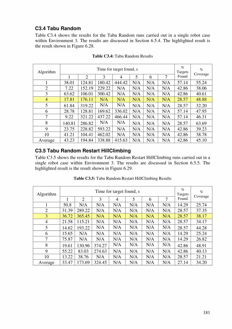
181
C3.4 Tabu Random
Table C3.4 shows the results for the Tabu Random runs carried out in a single robot case within Environment 3. The results are discussed in Section 6.5.4. The highlighted result is the result shown in Figure 6.28.
Table C3.4: Tabu Random Results
Time for target found, s Algorithm
1 2 3 4 5 6 7
% Targets Found
% Coverage
1 38.01 124.81 180.42 444.42 N/A N/A N/A 57.14 55.24 2 7.22 152.19 229.22 N/A N/A N/A N/A 42.86 38.06 3 63.62 106.01 300.42 N/A N/A N/A N/A 42.86 40.61 4 17.81 176.11 N/A N/A N/A N/A N/A 28.57 48.88 5 61.84 319.22 N/A N/A N/A N/A N/A 28.57 32.20 6 28.78 128.81 169.62 336.02 N/A N/A N/A 57.14 47.95 7 9.22 321.22 437.22 466.44 N/A N/A N/A 57.14 46.31 8 140.81 286.82 N/A N/A N/A N/A N/A 28.57 63.69 9 23.75 228.82 593.22 N/A N/A N/A N/A 42.86 39.23
10 41.21 104.41 462.02 N/A N/A N/A N/A 42.86 38.78 Average 43.23 194.84 338.88 415.63 N/A N/A N/A 42.86 45.10
C3.5 Tabu Random Restart HillClimbing
Table C3.5 shows the results for the Tabu Random Restart HillClimbing runs carried out in a single robot case within Environment 3. The results are discussed in Section 6.5.5. The highlighted result is the result shown in Figure 6.29.
Table C3.5: Tabu Random Restart HillClimbing Results
Time for target found, s Algorithm
1 2 3 4 5 6 7
% Targets Found
% Coverage
1 50.8 N/A N/A N/A N/A N/A N/A 14.29 25.74 2 31.39 289.22 N/A N/A N/A N/A N/A 28.57 37.35 3 36.72 365.45 N/A N/A N/A N/A N/A 28.57 38.17 4 21.58 115.21 N/A N/A N/A N/A N/A 28.57 34.17 5 14.62 193.22 N/A N/A N/A N/A N/A 28.57 44.28 6 15.65 N/A N/A N/A N/A N/A N/A 14.29 25.24 7 75.87 N/A N/A N/A N/A N/A N/A 14.29 26.82 8 19.61 130.96 374.27 N/A N/A N/A N/A 42.86 48.91 9 55.22 83.03 274.63 N/A N/A N/A N/A 42.86 40.13
10 13.22 38.76 N/A N/A N/A N/A N/A 28.57 21.21 Average 33.47 173.69 324.45 N/A N/A N/A N/A 27.14 34.20
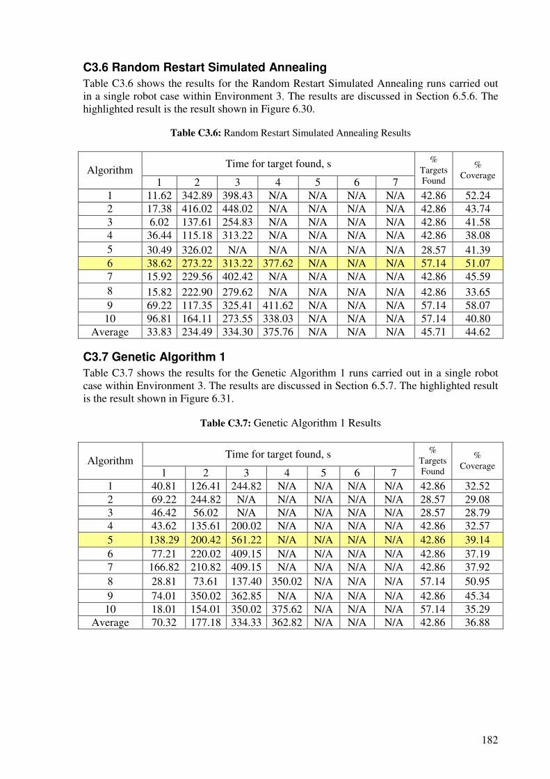
182
C3.6 Random Restart Simulated Annealing
Table C3.6 shows the results for the Random Restart Simulated Annealing runs carried out in a single robot case within Environment 3. The results are discussed in Section 6.5.6. The highlighted result is the result shown in Figure 6.30.
Table C3.6: Random Restart Simulated Annealing Results
Time for target found, s Algorithm
1 2 3 4 5 6 7
% Targets Found
% Coverage
1 11.62 342.89 398.43 N/A N/A N/A N/A 42.86 52.24 2 17.38 416.02 448.02 N/A N/A N/A N/A 42.86 43.74 3 6.02 137.61 254.83 N/A N/A N/A N/A 42.86 41.58 4 36.44 115.18 313.22 N/A N/A N/A N/A 42.86 38.08 5 30.49 326.02 N/A N/A N/A N/A N/A 28.57 41.39 6 38.62 273.22 313.22 377.62 N/A N/A N/A 57.14 51.07 7 15.92 229.56 402.42 N/A N/A N/A N/A 42.86 45.59 8 15.82 222.90 279.62 N/A N/A N/A N/A 42.86 33.65 9 69.22 117.35 325.41 411.62 N/A N/A N/A 57.14 58.07
10 96.81 164.11 273.55 338.03 N/A N/A N/A 57.14 40.80 Average 33.83 234.49 334.30 375.76 N/A N/A N/A 45.71 44.62
C3.7 Genetic Algorithm 1
Table C3.7 shows the results for the Genetic Algorithm 1 runs carried out in a single robot case within Environment 3. The results are discussed in Section 6.5.7. The highlighted result is the result shown in Figure 6.31.
Table C3.7: Genetic Algorithm 1 Results
Time for target found, s Algorithm
1 2 3 4 5 6 7
% Targets Found
% Coverage
1 40.81 126.41 244.82 N/A N/A N/A N/A 42.86 32.52 2 69.22 244.82 N/A N/A N/A N/A N/A 28.57 29.08 3 46.42 56.02 N/A N/A N/A N/A N/A 28.57 28.79 4 43.62 135.61 200.02 N/A N/A N/A N/A 42.86 32.57 5 138.29 200.42 561.22 N/A N/A N/A N/A 42.86 39.14 6 77.21 220.02 409.15 N/A N/A N/A N/A 42.86 37.19 7 166.82 210.82 409.15 N/A N/A N/A N/A 42.86 37.92 8 28.81 73.61 137.40 350.02 N/A N/A N/A 57.14 50.95 9 74.01 350.02 362.85 N/A N/A N/A N/A 42.86 45.34
10 18.01 154.01 350.02 375.62 N/A N/A N/A 57.14 35.29 Average 70.32 177.18 334.33 362.82 N/A N/A N/A 42.86 36.88
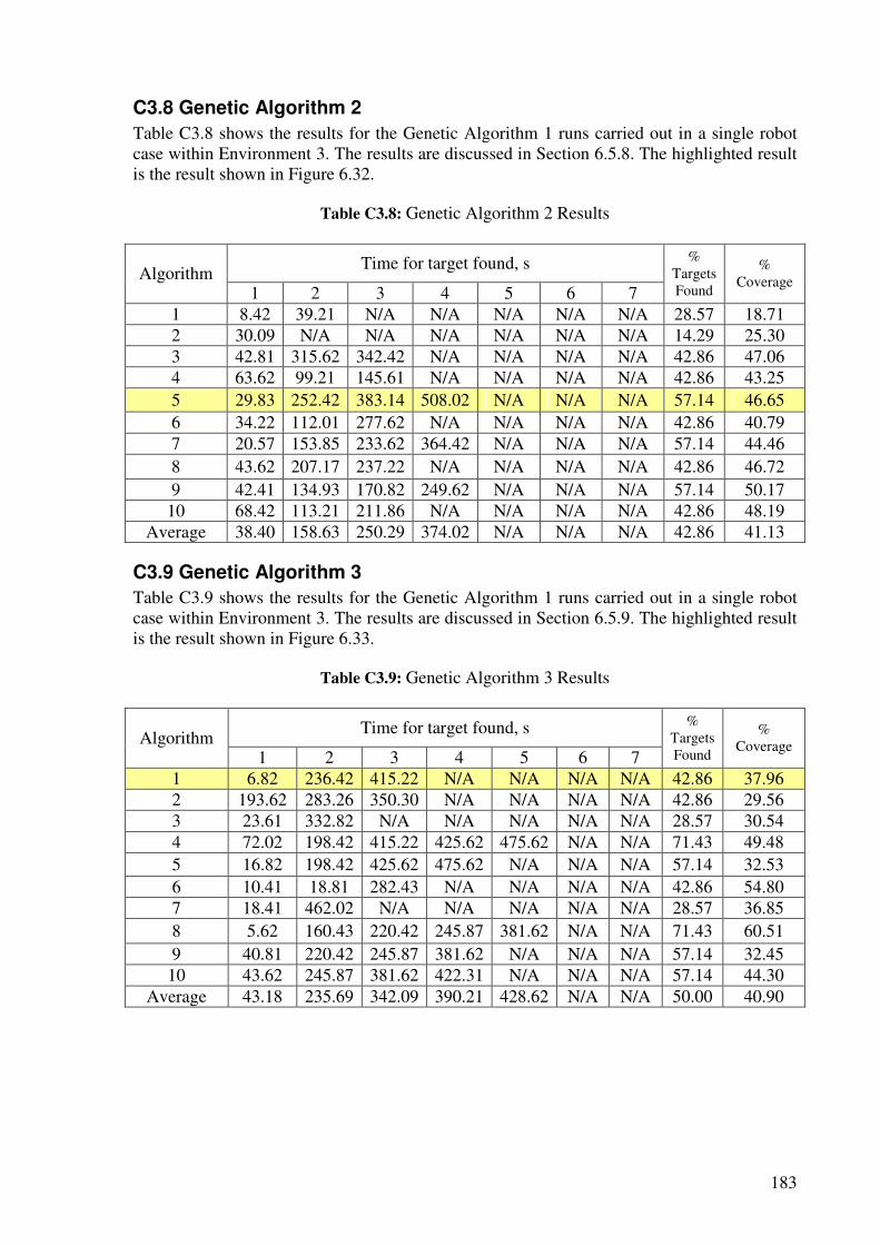
183
C3.8 Genetic Algorithm 2
Table C3.8 shows the results for the Genetic Algorithm 1 runs carried out in a single robot case within Environment 3. The results are discussed in Section 6.5.8. The highlighted result is the result shown in Figure 6.32.
Table C3.8: Genetic Algorithm 2 Results
Time for target found, s Algorithm
1 2 3 4 5 6 7
% Targets Found
% Coverage
1 8.42 39.21 N/A N/A N/A N/A N/A 28.57 18.71 2 30.09 N/A N/A N/A N/A N/A N/A 14.29 25.30 3 42.81 315.62 342.42 N/A N/A N/A N/A 42.86 47.06 4 63.62 99.21 145.61 N/A N/A N/A N/A 42.86 43.25 5 29.83 252.42 383.14 508.02 N/A N/A N/A 57.14 46.65 6 34.22 112.01 277.62 N/A N/A N/A N/A 42.86 40.79 7 20.57 153.85 233.62 364.42 N/A N/A N/A 57.14 44.46 8 43.62 207.17 237.22 N/A N/A N/A N/A 42.86 46.72 9 42.41 134.93 170.82 249.62 N/A N/A N/A 57.14 50.17
10 68.42 113.21 211.86 N/A N/A N/A N/A 42.86 48.19 Average 38.40 158.63 250.29 374.02 N/A N/A N/A 42.86 41.13
C3.9 Genetic Algorithm 3
Table C3.9 shows the results for the Genetic Algorithm 1 runs carried out in a single robot case within Environment 3. The results are discussed in Section 6.5.9. The highlighted result is the result shown in Figure 6.33.
Table C3.9: Genetic Algorithm 3 Results
Time for target found, s Algorithm
1 2 3 4 5 6 7
% Targets Found
% Coverage
1 6.82 236.42 415.22 N/A N/A N/A N/A 42.86 37.96 2 193.62 283.26 350.30 N/A N/A N/A N/A 42.86 29.56 3 23.61 332.82 N/A N/A N/A N/A N/A 28.57 30.54 4 72.02 198.42 415.22 425.62 475.62 N/A N/A 71.43 49.48 5 16.82 198.42 425.62 475.62 N/A N/A N/A 57.14 32.53 6 10.41 18.81 282.43 N/A N/A N/A N/A 42.86 54.80 7 18.41 462.02 N/A N/A N/A N/A N/A 28.57 36.85 8 5.62 160.43 220.42 245.87 381.62 N/A N/A 71.43 60.51 9 40.81 220.42 245.87 381.62 N/A N/A N/A 57.14 32.45
10 43.62 245.87 381.62 422.31 N/A N/A N/A 57.14 44.30 Average 43.18 235.69 342.09 390.21 428.62 N/A N/A 50.00 40.90
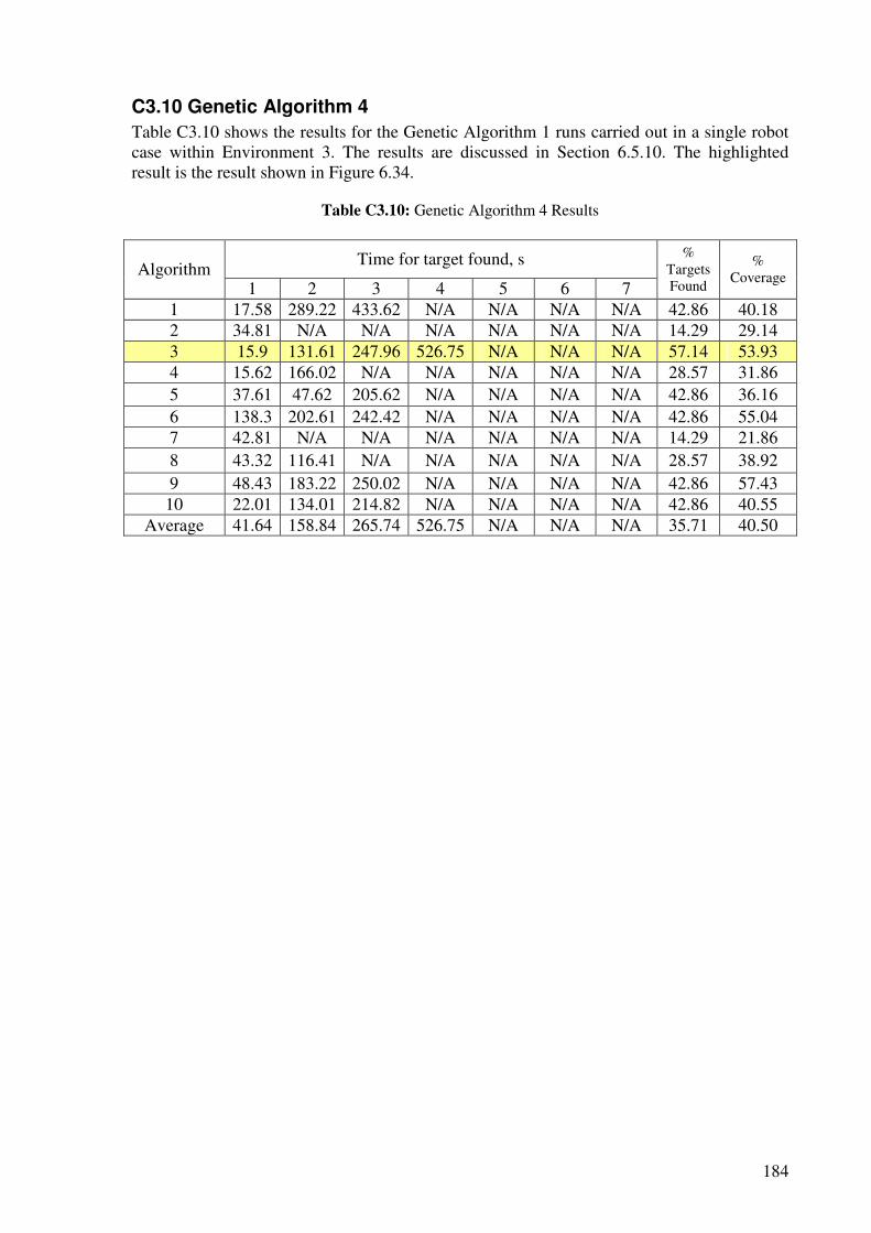
184
C3.10 Genetic Algorithm 4
Table C3.10 shows the results for the Genetic Algorithm 1 runs carried out in a single robot case within Environment 3. The results are discussed in Section 6.5.10. The highlighted result is the result shown in Figure 6.34.
Table C3.10: Genetic Algorithm 4 Results
Time for target found, s Algorithm
1 2 3 4 5 6 7
% Targets Found
% Coverage
1 17.58 289.22 433.62 N/A N/A N/A N/A 42.86 40.18 2 34.81 N/A N/A N/A N/A N/A N/A 14.29 29.14 3 15.9 131.61 247.96 526.75 N/A N/A N/A 57.14 53.93 4 15.62 166.02 N/A N/A N/A N/A N/A 28.57 31.86 5 37.61 47.62 205.62 N/A N/A N/A N/A 42.86 36.16 6 138.3 202.61 242.42 N/A N/A N/A N/A 42.86 55.04 7 42.81 N/A N/A N/A N/A N/A N/A 14.29 21.86 8 43.32 116.41 N/A N/A N/A N/A N/A 28.57 38.92 9 48.43 183.22 250.02 N/A N/A N/A N/A 42.86 57.43
10 22.01 134.01 214.82 N/A N/A N/A N/A 42.86 40.55 Average 41.64 158.84 265.74 526.75 N/A N/A N/A 35.71 40.50
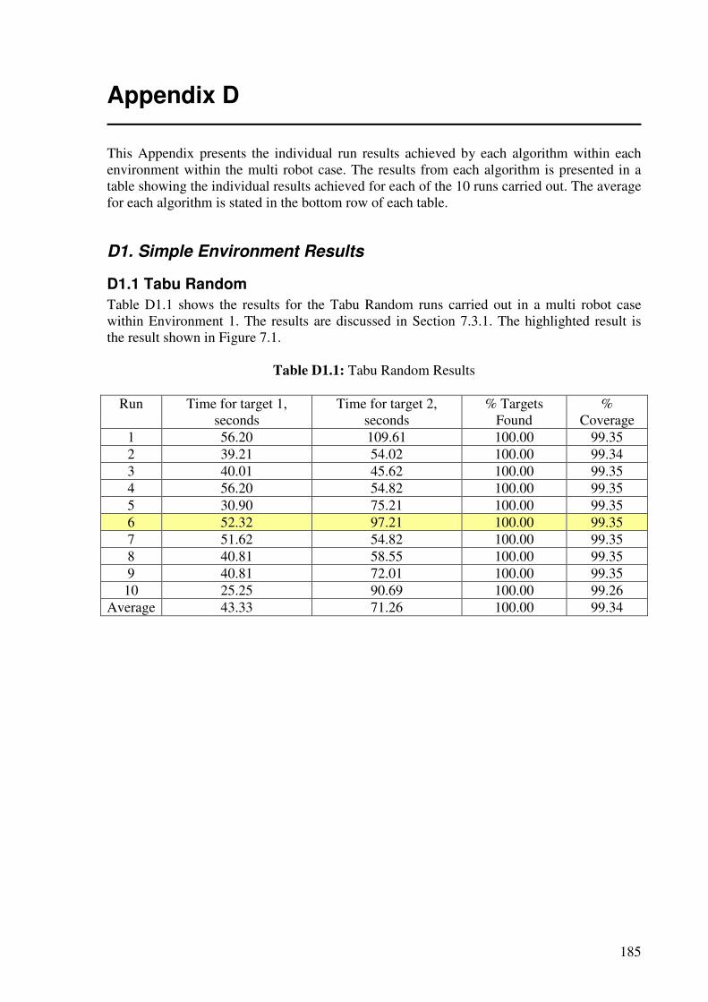
185
Appendix D
This Appendix presents the individual run results achieved by each algorithm within each environment within the multi robot case. The results from each algorithm is presented in a table showing the individual results achieved for each of the 10 runs carried out. The average for each algorithm is stated in the bottom row of each table.
D1. Simple Environment Results
D1.1 Tabu Random
Table D1.1 shows the results for the Tabu Random runs carried out in a multi robot case within Environment 1. The results are discussed in Section 7.3.1. The highlighted result is the result shown in Figure 7.1.
Table D1.1: Tabu Random Results
Run Time for target 1, seconds
Time for target 2, seconds
% Targets Found
% Coverage
1 56.20 109.61 100.00 99.35 2 39.21 54.02 100.00 99.34 3 40.01 45.62 100.00 99.35 4 56.20 54.82 100.00 99.35 5 30.90 75.21 100.00 99.35 6 52.32 97.21 100.00 99.35 7 51.62 54.82 100.00 99.35 8 40.81 58.55 100.00 99.35 9 40.81 72.01 100.00 99.35
10 25.25 90.69 100.00 99.26 Average 43.33 71.26 100.00 99.34
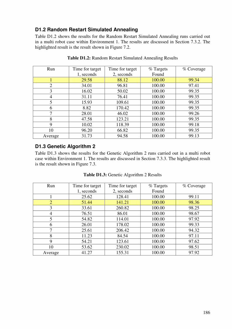
186
D1.2 Random Restart Simulated Annealing
Table D1.2 shows the results for the Random Restart Simulated Annealing runs carried out in a multi robot case within Environment 1. The results are discussed in Section 7.3.2. The highlighted result is the result shown in Figure 7.2.
Table D1.2: Random Restart Simulated Annealing Results
Run Time for target 1, seconds
Time for target 2, seconds
% Targets Found
% Coverage
1 29.58 88.12 100.00 99.34 2 34.01 96.81 100.00 97.41 3 16.02 50.02 100.00 99.35 4 31.11 76.41 100.00 99.35 5 15.93 109.61 100.00 99.35 6 8.82 170.42 100.00 99.35 7 28.01 46.02 100.00 99.26 8 47.58 123.21 100.00 99.35 9 10.02 118.39 100.00 99.18
10 96.20 66.82 100.00 99.35 Average 31.73 94.58 100.00 99.13
D1.3 Genetic Algorithm 2
Table D1.3 shows the results for the Genetic Algorithm 2 runs carried out in a multi robot case within Environment 1. The results are discussed in Section 7.3.3. The highlighted result is the result shown in Figure 7.3.
Table D1.3: Genetic Algorithm 2 Results
Run Time for target 1, seconds
Time for target 2, seconds
% Targets Found
% Coverage
1 25.62 128.41 100.00 99.11 2 51.44 141.21 100.00 98.36 3 33.61 260.82 100.00 98.25 4 76.51 86.01 100.00 98.67 5 54.82 114.01 100.00 97.92 6 26.01 178.02 100.00 99.33 7 25.61 206.42 100.00 94.32 8 11.23 84.54 100.00 97.11 9 54.21 123.61 100.00 97.62
10 53.62 230.02 100.00 98.51 Average 41.27 155.31 100.00 97.92
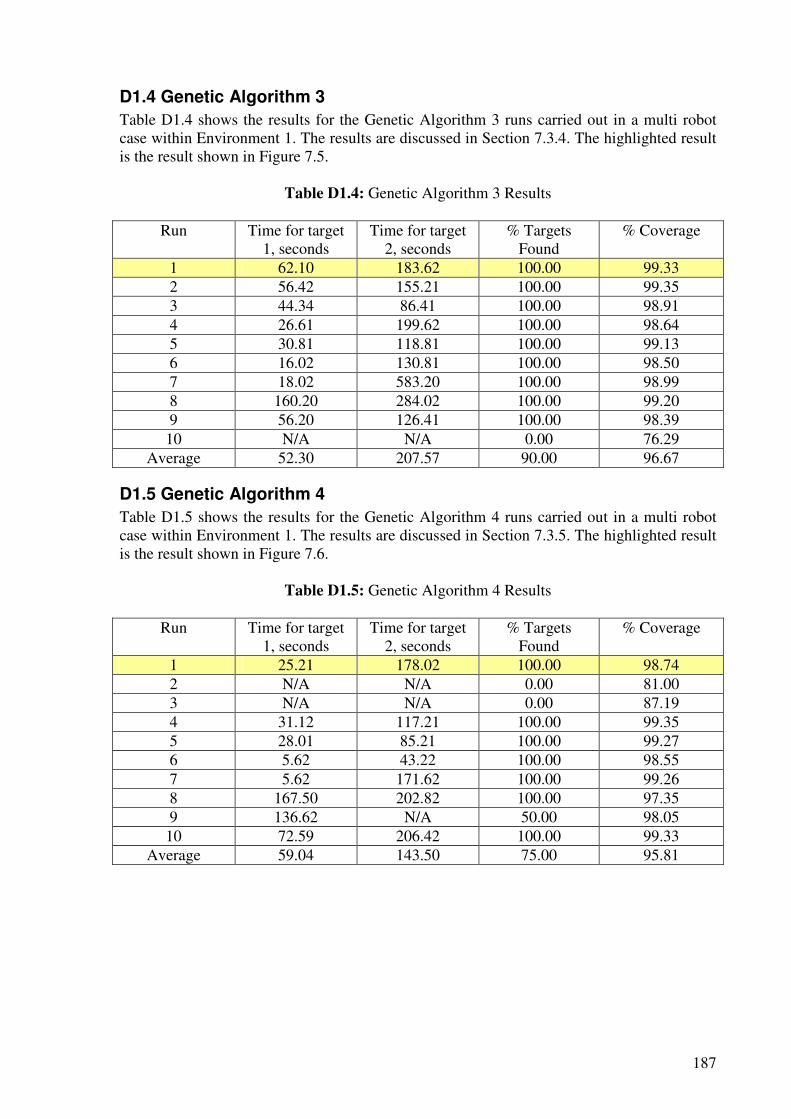
187
D1.4 Genetic Algorithm 3
Table D1.4 shows the results for the Genetic Algorithm 3 runs carried out in a multi robot case within Environment 1. The results are discussed in Section 7.3.4. The highlighted result is the result shown in Figure 7.5.
Table D1.4: Genetic Algorithm 3 Results
Run Time for target 1, seconds
Time for target 2, seconds
% Targets Found
% Coverage
1 62.10 183.62 100.00 99.33 2 56.42 155.21 100.00 99.35 3 44.34 86.41 100.00 98.91 4 26.61 199.62 100.00 98.64 5 30.81 118.81 100.00 99.13 6 16.02 130.81 100.00 98.50 7 18.02 583.20 100.00 98.99 8 160.20 284.02 100.00 99.20 9 56.20 126.41 100.00 98.39
10 N/A N/A 0.00 76.29 Average 52.30 207.57 90.00 96.67
D1.5 Genetic Algorithm 4
Table D1.5 shows the results for the Genetic Algorithm 4 runs carried out in a multi robot case within Environment 1. The results are discussed in Section 7.3.5. The highlighted result is the result shown in Figure 7.6.
Table D1.5: Genetic Algorithm 4 Results
Run Time for target
1, seconds Time for target
2, seconds % Targets
Found % Coverage
1 25.21 178.02 100.00 98.74 2 N/A N/A 0.00 81.00 3 N/A N/A 0.00 87.19 4 31.12 117.21 100.00 99.35 5 28.01 85.21 100.00 99.27 6 5.62 43.22 100.00 98.55 7 5.62 171.62 100.00 99.26 8 167.50 202.82 100.00 97.35 9 136.62 N/A 50.00 98.05
10 72.59 206.42 100.00 99.33 Average 59.04 143.50 75.00 95.81
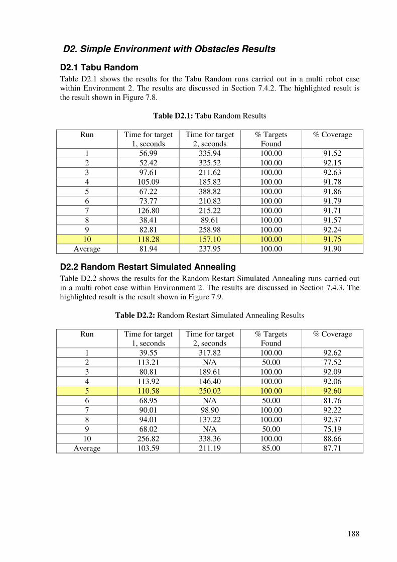
188
D2. Simple Environment with Obstacles Results
D2.1 Tabu Random
Table D2.1 shows the results for the Tabu Random runs carried out in a multi robot case within Environment 2. The results are discussed in Section 7.4.2. The highlighted result is the result shown in Figure 7.8.
Table D2.1: Tabu Random Results
Run Time for target 1, seconds
Time for target 2, seconds
% Targets Found
% Coverage
1 56.99 335.94 100.00 91.52 2 52.42 325.52 100.00 92.15 3 97.61 211.62 100.00 92.63 4 105.09 185.82 100.00 91.78 5 67.22 388.82 100.00 91.86 6 73.77 210.82 100.00 91.79 7 126.80 215.22 100.00 91.71 8 38.41 89.61 100.00 91.57 9 82.81 258.98 100.00 92.24
10 118.28 157.10 100.00 91.75 Average 81.94 237.95 100.00 91.90
D2.2 Random Restart Simulated Annealing
Table D2.2 shows the results for the Random Restart Simulated Annealing runs carried out in a multi robot case within Environment 2. The results are discussed in Section 7.4.3. The highlighted result is the result shown in Figure 7.9.
Table D2.2: Random Restart Simulated Annealing Results
Run Time for target 1, seconds
Time for target 2, seconds
% Targets Found
% Coverage
1 39.55 317.82 100.00 92.62 2 113.21 N/A 50.00 77.52 3 80.81 189.61 100.00 92.09 4 113.92 146.40 100.00 92.06 5 110.58 250.02 100.00 92.60 6 68.95 N/A 50.00 81.76 7 90.01 98.90 100.00 92.22 8 94.01 137.22 100.00 92.37 9 68.02 N/A 50.00 75.19
10 256.82 338.36 100.00 88.66 Average 103.59 211.19 85.00 87.71
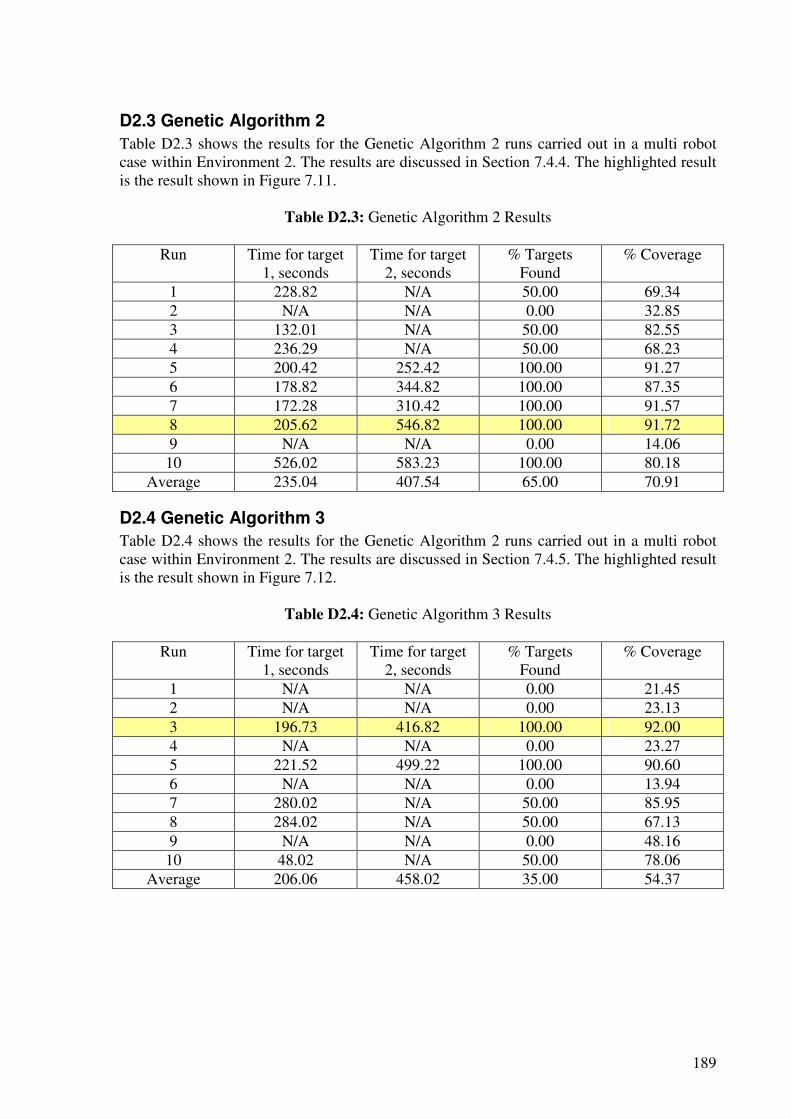
189
D2.3 Genetic Algorithm 2
Table D2.3 shows the results for the Genetic Algorithm 2 runs carried out in a multi robot case within Environment 2. The results are discussed in Section 7.4.4. The highlighted result is the result shown in Figure 7.11.
Table D2.3: Genetic Algorithm 2 Results
Run Time for target 1, seconds
Time for target 2, seconds
% Targets Found
% Coverage
1 228.82 N/A 50.00 69.34 2 N/A N/A 0.00 32.85 3 132.01 N/A 50.00 82.55 4 236.29 N/A 50.00 68.23 5 200.42 252.42 100.00 91.27 6 178.82 344.82 100.00 87.35 7 172.28 310.42 100.00 91.57 8 205.62 546.82 100.00 91.72 9 N/A N/A 0.00 14.06
10 526.02 583.23 100.00 80.18 Average 235.04 407.54 65.00 70.91
D2.4 Genetic Algorithm 3
Table D2.4 shows the results for the Genetic Algorithm 2 runs carried out in a multi robot case within Environment 2. The results are discussed in Section 7.4.5. The highlighted result is the result shown in Figure 7.12.
Table D2.4: Genetic Algorithm 3 Results
Run Time for target 1, seconds
Time for target 2, seconds
% Targets Found
% Coverage
1 N/A N/A 0.00 21.45 2 N/A N/A 0.00 23.13 3 196.73 416.82 100.00 92.00 4 N/A N/A 0.00 23.27 5 221.52 499.22 100.00 90.60 6 N/A N/A 0.00 13.94 7 280.02 N/A 50.00 85.95 8 284.02 N/A 50.00 67.13 9 N/A N/A 0.00 48.16
10 48.02 N/A 50.00 78.06 Average 206.06 458.02 35.00 54.37
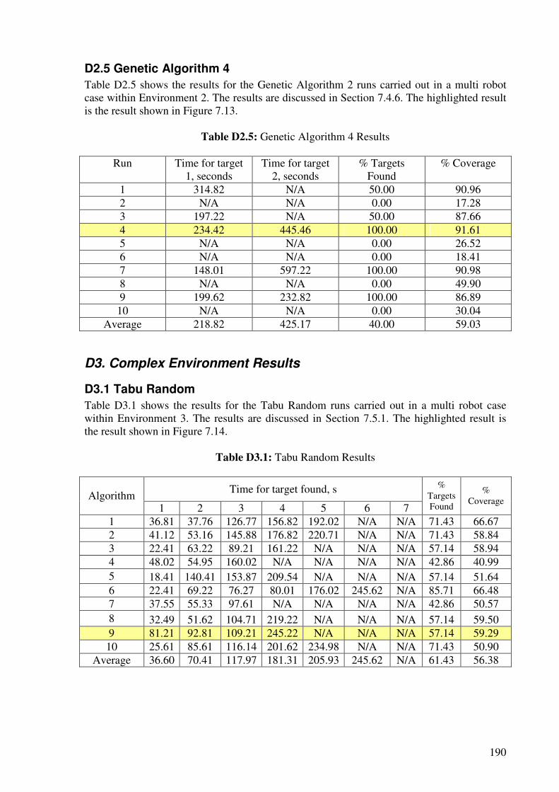
190
D2.5 Genetic Algorithm 4
Table D2.5 shows the results for the Genetic Algorithm 2 runs carried out in a multi robot case within Environment 2. The results are discussed in Section 7.4.6. The highlighted result is the result shown in Figure 7.13.
Table D2.5: Genetic Algorithm 4 Results
Run Time for target 1, seconds
Time for target 2, seconds
% Targets Found
% Coverage
1 314.82 N/A 50.00 90.96 2 N/A N/A 0.00 17.28 3 197.22 N/A 50.00 87.66 4 234.42 445.46 100.00 91.61 5 N/A N/A 0.00 26.52 6 N/A N/A 0.00 18.41 7 148.01 597.22 100.00 90.98 8 N/A N/A 0.00 49.90 9 199.62 232.82 100.00 86.89
10 N/A N/A 0.00 30.04 Average 218.82 425.17 40.00 59.03
D3. Complex Environment Results
D3.1 Tabu Random
Table D3.1 shows the results for the Tabu Random runs carried out in a multi robot case within Environment 3. The results are discussed in Section 7.5.1. The highlighted result is the result shown in Figure 7.14.
Table D3.1: Tabu Random Results
Time for target found, s Algorithm
1 2 3 4 5 6 7
% Targets Found
% Coverage
1 36.81 37.76 126.77 156.82 192.02 N/A N/A 71.43 66.67 2 41.12 53.16 145.88 176.82 220.71 N/A N/A 71.43 58.84 3 22.41 63.22 89.21 161.22 N/A N/A N/A 57.14 58.94 4 48.02 54.95 160.02 N/A N/A N/A N/A 42.86 40.99 5 18.41 140.41 153.87 209.54 N/A N/A N/A 57.14 51.64 6 22.41 69.22 76.27 80.01 176.02 245.62 N/A 85.71 66.48 7 37.55 55.33 97.61 N/A N/A N/A N/A 42.86 50.57 8 32.49 51.62 104.71 219.22 N/A N/A N/A 57.14 59.50 9 81.21 92.81 109.21 245.22 N/A N/A N/A 57.14 59.29
10 25.61 85.61 116.14 201.62 234.98 N/A N/A 71.43 50.90 Average 36.60 70.41 117.97 181.31 205.93 245.62 N/A 61.43 56.38
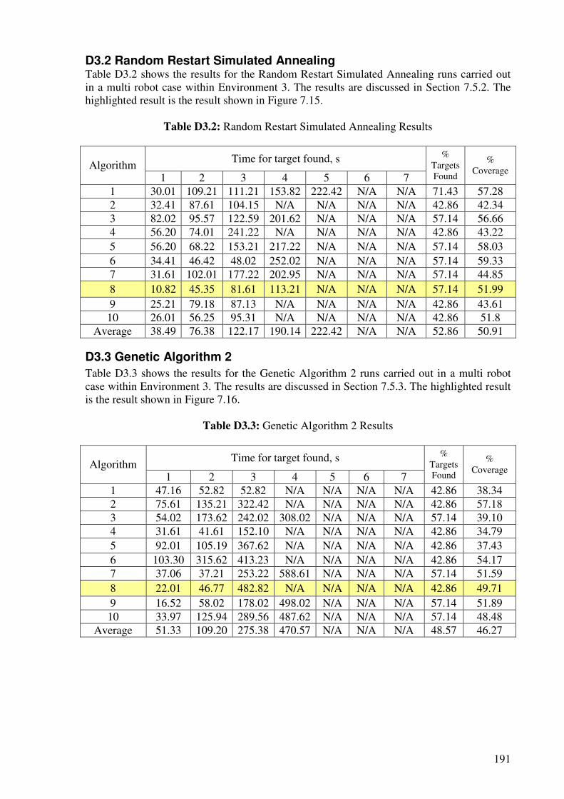
191
D3.2 Random Restart Simulated Annealing Table D3.2 shows the results for the Random Restart Simulated Annealing runs carried out in a multi robot case within Environment 3. The results are discussed in Section 7.5.2. The highlighted result is the result shown in Figure 7.15.
Table D3.2: Random Restart Simulated Annealing Results
Time for target found, s Algorithm
1 2 3 4 5 6 7
% Targets Found
% Coverage
1 30.01 109.21 111.21 153.82 222.42 N/A N/A 71.43 57.28 2 32.41 87.61 104.15 N/A N/A N/A N/A 42.86 42.34 3 82.02 95.57 122.59 201.62 N/A N/A N/A 57.14 56.66 4 56.20 74.01 241.22 N/A N/A N/A N/A 42.86 43.22 5 56.20 68.22 153.21 217.22 N/A N/A N/A 57.14 58.03 6 34.41 46.42 48.02 252.02 N/A N/A N/A 57.14 59.33 7 31.61 102.01 177.22 202.95 N/A N/A N/A 57.14 44.85 8 10.82 45.35 81.61 113.21 N/A N/A N/A 57.14 51.99 9 25.21 79.18 87.13 N/A N/A N/A N/A 42.86 43.61
10 26.01 56.25 95.31 N/A N/A N/A N/A 42.86 51.8 Average 38.49 76.38 122.17 190.14 222.42 N/A N/A 52.86 50.91
D3.3 Genetic Algorithm 2
Table D3.3 shows the results for the Genetic Algorithm 2 runs carried out in a multi robot case within Environment 3. The results are discussed in Section 7.5.3. The highlighted result is the result shown in Figure 7.16.
Table D3.3: Genetic Algorithm 2 Results
Time for target found, s Algorithm
1 2 3 4 5 6 7
% Targets Found
% Coverage
1 47.16 52.82 52.82 N/A N/A N/A N/A 42.86 38.34 2 75.61 135.21 322.42 N/A N/A N/A N/A 42.86 57.18 3 54.02 173.62 242.02 308.02 N/A N/A N/A 57.14 39.10 4 31.61 41.61 152.10 N/A N/A N/A N/A 42.86 34.79 5 92.01 105.19 367.62 N/A N/A N/A N/A 42.86 37.43 6 103.30 315.62 413.23 N/A N/A N/A N/A 42.86 54.17 7 37.06 37.21 253.22 588.61 N/A N/A N/A 57.14 51.59 8 22.01 46.77 482.82 N/A N/A N/A N/A 42.86 49.71 9 16.52 58.02 178.02 498.02 N/A N/A N/A 57.14 51.89
10 33.97 125.94 289.56 487.62 N/A N/A N/A 57.14 48.48 Average 51.33 109.20 275.38 470.57 N/A N/A N/A 48.57 46.27
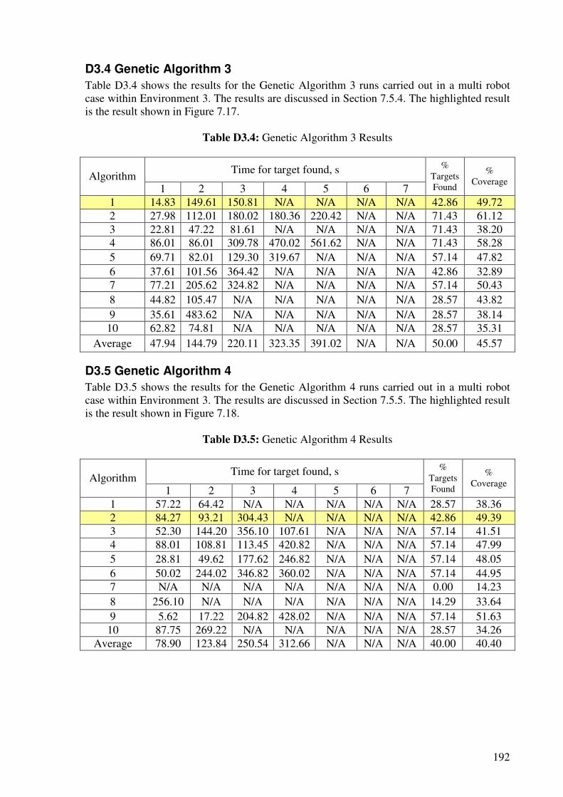
192
D3.4 Genetic Algorithm 3
Table D3.4 shows the results for the Genetic Algorithm 3 runs carried out in a multi robot case within Environment 3. The results are discussed in Section 7.5.4. The highlighted result is the result shown in Figure 7.17.
Table D3.4: Genetic Algorithm 3 Results
Time for target found, s Algorithm
1 2 3 4 5 6 7
% Targets Found
% Coverage
1 14.83 149.61 150.81 N/A N/A N/A N/A 42.86 49.72 2 27.98 112.01 180.02 180.36 220.42 N/A N/A 71.43 61.12 3 22.81 47.22 81.61 N/A N/A N/A N/A 71.43 38.20 4 86.01 86.01 309.78 470.02 561.62 N/A N/A 71.43 58.28 5 69.71 82.01 129.30 319.67 N/A N/A N/A 57.14 47.82 6 37.61 101.56 364.42 N/A N/A N/A N/A 42.86 32.89 7 77.21 205.62 324.82 N/A N/A N/A N/A 57.14 50.43 8 44.82 105.47 N/A N/A N/A N/A N/A 28.57 43.82 9 35.61 483.62 N/A N/A N/A N/A N/A 28.57 38.14
10 62.82 74.81 N/A N/A N/A N/A N/A 28.57 35.31 Average 47.94 144.79 220.11 323.35 391.02 N/A N/A 50.00 45.57
D3.5 Genetic Algorithm 4
Table D3.5 shows the results for the Genetic Algorithm 4 runs carried out in a multi robot case within Environment 3. The results are discussed in Section 7.5.5. The highlighted result is the result shown in Figure 7.18.
Table D3.5: Genetic Algorithm 4 Results
Time for target found, s Algorithm
1 2 3 4 5 6 7
% Targets Found
% Coverage
1 57.22 64.42 N/A N/A N/A N/A N/A 28.57 38.36 2 84.27 93.21 304.43 N/A N/A N/A N/A 42.86 49.39 3 52.30 144.20 356.10 107.61 N/A N/A N/A 57.14 41.51 4 88.01 108.81 113.45 420.82 N/A N/A N/A 57.14 47.99 5 28.81 49.62 177.62 246.82 N/A N/A N/A 57.14 48.05 6 50.02 244.02 346.82 360.02 N/A N/A N/A 57.14 44.95 7 N/A N/A N/A N/A N/A N/A N/A 0.00 14.23 8 256.10 N/A N/A N/A N/A N/A N/A 14.29 33.64 9 5.62 17.22 204.82 428.02 N/A N/A N/A 57.14 51.63
10 87.75 269.22 N/A N/A N/A N/A N/A 28.57 34.26 Average 78.90 123.84 250.54 312.66 N/A N/A N/A 40.00 40.40
Related Documents