Guaranteeing Convergence of Iterative Skewed Voting Algorithms for Image Segmentation

arX

iv:1

102.

2615

v2 [

mat

h.F

A]

21 F

eb 2

011

Guaranteeing Convergence of Iterative Skewed Voting Algorithmsfor Image Segmentation

Doru C. Balcana,∗, Gowri Srinivasab, Matthew Fickusc, Jelena Kovacevicd

aSchool of Interactive Computing, Georgia Institute of Technology, Atlanta, USAbDept. of Information Science and Engineering, and Center for Pattern Recognition, PES School of Engineering, Bangalore, India

cDept. of Mathematics and Statistics, Air Force Institute ofTechnology, Wright-Patterson AFB, USAdDept. of Biomedical Eng., Electrical and Computer Eng. and Center for Bioimage Informatics, Carnegie Mellon University, Pittsburgh, USA

Abstract

In this paper we provide rigorous proof for the convergence of an iterative voting-based image segmentation algorithmcalled Active Masks. Active Masks (AM) was proposed to solvethe challenging task of delineating punctate patternsof cells from fluorescence microscope images. Each iteration of AM consists of a linear convolution composed witha nonlinear thresholding; what makes this process special in our case is the presence of additive terms whose role isto "skew" the voting when prior information is available. Inreal-world implementation, the AM algorithm alwaysconverges to a fixed point. We study the behavior of AM rigorously and present a proof of this convergence. Thekey idea is to formulate AM as a generalized (parallel) majority cellular automaton, adapting proof techniques fromdiscrete dynamical systems.

Keywords: active masks, cellular automata, convergence, segmentation.

1. Introduction

Recently, a new algorithm calledActive Masks(AM) was proposed for the segmentation of biological images[14].Let the “image” f be any real-valued function over the domainΩ :=

∏Dd=1 ZNd and refer to theN := N1N2. . .ND

elements ofΩ aspixels; here,ZNd denotes the finite group of integers moduloNd. A segmentationof f assigns one ofM possiblelabelsto each of theN pixels inΩ. For the fluorescence microscope image depicted in Figure 1(a), oneexample of a successful segmentation is to label all of the background pixels as “1,” assign label “2” to every pixel inthe largest cell, “3” to every pixel in the second largest cell, and so on. Formally, a segmentation is alabel functionψ : Ω → 1, 2, . . . ,M, or, equivalently, a collection ofM binarymasksµm : Ω → 0, 1 where, at any givenn ∈ Ω,we haveµm(n) = 1 if and only ifψ(n) = m. That is,µm at any iterationi can be defined as

µ(i)m :=

1, ψi(n) = m,0, ψi(n) , m,

In AM, these masks actively evolve according to a given rule.To understand this evolution, it helps to first discussiterative voting: in each iteration, at any given pixel, one counts how often agiven label appears in the neighborhoodof that pixel—weighting nearby neighbors more than distantones—and assigns the most frequent label to that pixelin the next iteration. For example, if a pixel labeled “1” in the current iteration is completely surrounded by pixelslabeled “2”, its label will likely change to “2” in the next iteration. Formally speaking, iterative voting is the repeatedapplication of the rule:

Iterative Voting: ψi(n) = argmax1≤m≤M

[

(µ(i−1)m ∗ g)(n)

]

, (1)

∗Corresponding authorEmail addresses:[email protected] (Doru C. Balcan),[email protected] (Gowri Srinivasa),[email protected]

(Matthew Fickus),[email protected] (Jelena Kovacevic)1Email: [email protected]. Mailing address: College of Computing Building, room 218, Georgia Institute of Technology, 801 Atlantic

Drive, Atlanta, GA 30332-0280. Phone: (404) 385-8547, Fax:(404)894-0673.

Preprint submitted to Elsevier February 22, 2011

wherei is the index of the iteration,g : Ω → R is some arbitrarily chosen fixed weighting function and “∗” denotescircular convolution overΩ. Iterative voting is referred to as aconvolution-thresholdscheme since it simplifies torounding the filtered version ofµ(i)

1 in the special caseM = 2. Experimentation reveals that for typical low-pass filtersg, repeatedly applying (1) to a given initialψ0 results in a progressive smoothing of the contours between distinctlylabeled regions ofΩ. Despite this nice property, note that taken by itself, iterative voting is useless as a segmentationscheme, as (1) evolves masks in a manner that is independent of any image under consideration.

The AM algorithm is a generalization of (1) that contains additional image-based terms whose purpose is to drivethe iteration towards a meaningful segmentation. To be precise, the AM iteration is:

Active Masks: ψi(n) = argmax1≤m≤M

[

(µ(i−1)m ∗ g)(n) + Rm(n)

]

, (2)

where the region-based distributing functionsRmMm=1 can be any image-dependent real-valued functions overΩ.

These will be referred to asskew functionsin this paper, due to their role to bias the voting. Essentially, at any givenpixel n, these additional terms skew the voting towards labelsmwhoseRm(n) values are large. For good segmentation,one should define theRm’s in terms of features in the image that distinguish regionsof interest from each other.

For example, for the fluorescence microscope image given in Figure 1(a), the cells appear noticeably brighter thanthe background. As such, we chooseR1 to be a soft-thresholded version of the image’s local average brightness, andchoose the remainingRm’s to be identically zero. When (2) is applied, such a choice in Rm’s forces pixels which lieoutside the cells towards label “1,” while pixels that lie inside a cell can assume any other label. Intuitively, repeatedapplications of (2) will cause the maskµ(i)

1 to converge to an indicator function of the background, while each ofthe other masksµ(i)

m Mm=2 converges either to a smooth blob contained within the foreground or to the empty set.

Experimentation reveals that the AM algorithm indeed oftenconverges to aψ which assigns a unique label to eachcell provided the scale of the windowg is chosen appropriately [14]; see Figure 1 for examples.

The purpose of this paper is to provide a rigorous investigation of the convergence behavior of the AM algorithm.To be precise, we note that in a real-world implementation the AM algorithm occasionally fails to converge to aψwhich is biologically meaningful. However, even in these cases, the algorithm always seems to converge to something.Indeed, whenψ0 and theRm’s are chosen at random, experimentation reveals that the repeated application of (2) alwaysseems to eventually produceψi such thatψi+1 = ψi . At the same time, a simple example tempers one’s expectations:takingΩ = Z4, M = 2, w = δ−1 + δ0 + δ1 andR1 = R2 = 0, we see that AM will not always converge, as repeatedlyapplying (2) toψ0 = δ0 + δ2 produces the endless 2-cycleδ0 + δ2 7→ δ1 + δ3 7→ δ0 + δ2. In summary, even thoughrandom experimentation indicates that AM will almost certainly converge, there exist trivial examples which showthat it will not always do so. The central question that this paper seeks to address is therefore:

Under what conditions ong andRmMm=1 will the AM algorithm always converge to a fixed point of (2) ?

We show that wheng is an even function, AM will either converge to a fixed point orwill get stuck in a 2-cycle;no higher-order cycles are possible. We can further rule out2-cycles wheneverg is taken so that the convolutionaloperatorf 7→ f ∗ g is positive semidefinite. The following is a compilation of these results:

Theorem 1.1. Given anyΩ :=∏D

d=1ZNd , initial segmentationψ0 : Ω → 1, . . . ,M and any real-valued functionsRm

Mm=1 overΩ, the Active Mask algorithm, namely the repeated application of (2), will always converge to a fixed

point of (2) provided the discrete Fourier transform of g is nonnegativeand even.

A preliminary version of the results in this paper appears inthe conference proceeding [2]. Though the specific AMalgorithm was introduced in [14], iterative lowpass filtering has long been a subject of interest in applied harmonicanalysis, having deep connections to continuous-domain ideas such as diffusion and the maximum principle [8].For instance, [9] gives an edge detection application of a discretized version of these ideas. Meanwhile, [6] givesdiffusion-inspired conditions under which lowpass filtering isguaranteed to produce a coarse version of a given image.One way to prove the convergence of iterative convolution-thresholding schemes is to show that lowpass filteringdecreases the number of zero-crossings in a signal; such a condition is equivalent to a version of the maximumprinciple [11]. More recently, the continuous-domain version of (1) has been used to model the motion of interfacesbetween media [12, 13]; in that setting, (1) is known to converge if M = 2. Since the AM algorithm is iterative, manyof the proof techniques we use here were adapted frommajority cellular automata(MCA), a well-studied class of

2

(a) Original image (b) i=0, M=256

scale= 4 scale= 16 scale= 32

Gaussian Filter

i = 2

i = 8

i = 14

Final state

(c) Segmentation outcomes for various scales

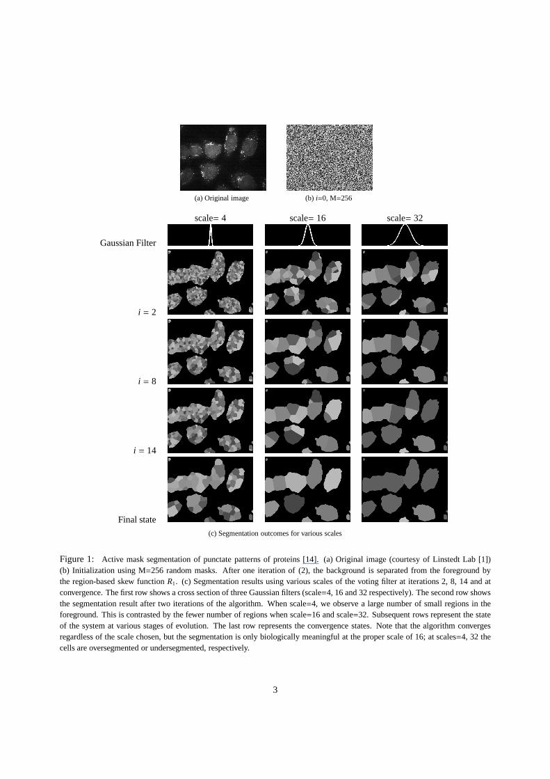
Figure 1: Active mask segmentation of punctate patterns of proteins [14]. (a) Original image (courtesy of Linstedt Lab [1])(b) Initialization using M=256 random masks. After one iteration of (2), the backgroundis separated from the foreground bythe region-based skew functionR1. (c) Segmentation results using various scales of the voting filter at iterations 2, 8, 14 and atconvergence. The first row shows a cross section of three Gaussian filters (scale=4, 16 and 32 respectively). The second row showsthe segmentation result after two iterations of the algorithm. When scale=4, we observe a large number of small regions in theforeground. This is contrasted by the fewer number of regions when scale=16 and scale=32. Subsequent rows represent the stateof the system at various stages of evolution. The last row represents the convergence states. Note that the algorithm convergesregardless of the scale chosen, but the segmentation is onlybiologically meaningful at the proper scale of 16; at scales=4, 32 thecells are oversegmented or undersegmented, respectively.

3

discrete dynamical systems. Indeed, theoretical guarantees on the convergence of a symmetric class of MCA havebeen known for several decades; see [3, 10], and references therein. Such results were recently generalized to a quasi-symmetric class via the use of Lyapunov functionals [7]. Whereas much of traditional MCA theory focuses on theconvergence of repeated applications of (1), our work differs due to the presence of the additiveRm terms in (2).

The paper is organized as follows. In the next section, we usean MCA formulation of AM to prove our mainconvergence results. In Section 3, we then briefly discuss the generalization of our main results to a less elegantyet more realistic version of (2) involving noncircular convolution. We conclude in Section 4 with some examplesillustrating our main results, as well as some experimentalresults indicating the AM algorithm’s rate of convergence.

2. Active Masks as a Majority Cellular Automaton

Cellular automata are self-evolving discrete dynamical systems [3]. They have been applied in various fields suchas statistical physics, computational biology, and the social sciences. A tremendous amount of work in this area hasfocused on studying the convergence behavior of various types of automata. In this section, we formulate the AMalgorithm (2) as an MCA in order to facilitate our understanding of its convergence behavior. To be precise, weconsider a generalization of (2) in which the convolutionaloperatorf 7→ f ∗ g may more broadly be taken to be anylinear operatorA from ℓ(Ω) := f | f : Ω→ R into itself:

ψi(n) := min(

argmaxm

[

(Aµ(i−1)m )(n) + Rm(n)

]

)

, µ(i−1)m :=

1, ψi−1(n) = m,0, ψi−1(n) , m.

(3)

Here, the contribution of maskm in deciding the outcome at locationn at iterationi is (Aµ(i−1)m )(n), and any ties are

broken by choosing the smallestm corresponding to a maximal element. Note that given any initial segmentationψ0,applying (3)ad infinitumproduces a sequenceψi

∞i=0. However, as there are onlyMN distinct possible configurations

for ψ : Ω→ 1, . . . ,M, this sequence must eventually repeat itself. Indeed, taking minimal indicesi0 andK > 0 suchthatψi0+K = ψi0, the deterministic nature of (3) implies thatψi+K = ψi for all i ≥ i0. The finite sequenceψi

i0+K−1i=i0

iscalled acycleof (3) of length K. Note thatψi

∞i=0 converges if and only ifK = 1, which happens precisely whenψi0

is a fixed point of (3).Thus, from this perspective, proving that (3) always converges is equivalent to proving thatK = 1 regardless of

one’s choice ofψ0. The following result goes a long way towards this goal, showing that if A is self-adjoint, then foranyψ0 we have that the resultingK is necessarily 1 or 2. That is, ifA is self-adjoint, then for anyψ0, the sequenceψi

∞i=0 will either converge in a finite number of iterations, or it will eventually come to a point where it forever

oscillates between two distinct configurationsψi0 andψi0+1.

Theorem 2.1. If A is self-adjoint, then for anyψ0, the cycle length K of(3) is either 1 or 2.

Proof. As we are not presently concerned with the rate of convergence of (3), but rather the question of whether itdoes converge, we may assume without loss of generality thatψi

∞i=0 has already entered its cycle. That is, we reindex

so thatψ0 is the beginning of theK-cycle, and heretofore regard all iteration indices as members of the cyclic groupZK . We argue by contrapositive, assumingK > 2 and concluding thatA is not self-adjoint. For anyi = 1, . . . ,K, (3)is equivalent to the system of inequalities:

(Aµ(i−1)ψi(n))(n) + Rψi(n)(n) > (Aµ(i−1)

m )(n) + Rm(n) if 1 ≤ m< ψi(n), (4a)

(Aµ(i−1)ψi(n))(n) + Rψi(n)(n) ≥ (Aµ(i−1)

m )(n) + Rm(n) if ψi(n) ≤ m≤ M. (4b)

Here, (4b) follows from the fact thatψi(n) is a value ofm that maximizes (Aµ(i−1)m )(n)+ Rm(n). Moreover, in the event

of a tie,ψi(n) is chosen to be the least of all such maximizingm, yielding the strict inequality in (4a). For anyi andn,pickingm= ψi−2(n) in (4a) and (4b) leads to the subsystem of inequalities:

(Aµ(i−1)ψi (n))(n) − (Aµ(i−1)

ψi−2(n))(n) + Rψi(n)(n) − Rψi−2(n)(n) > 0 if ψi−2(n) < ψi(n), (5a)

(Aµ(i−1)ψi (n))(n) − (Aµ(i−1)

ψi−2(n))(n) + Rψi(n)(n) − Rψi−2(n)(n) ≥ 0 if ψi−2(n) ≥ ψi(n). (5b)

4

Now sinceK > 2, there exists a pixeln for which ψ0(n), ψ1(n), . . . , ψK−1(n) is not of the forma, a, . . . , a nor ofthe forma, b, a, b, . . .a, b. At such ann, there must exist ani such thatψi−2(n) < ψi(n). Consequently, at least oneinequality in (5) is strict. Thus, summing (5) over all pixelsn and all cycle indicesi yields:

0 <∑

i∈ZK

∑

n∈Ω

(Aµ(i−1)ψi (n))(n) −

∑

i∈ZK

∑

n∈Ω

(Aµ(i−1)ψi−2(n))(n) +

∑

i∈ZK

∑

n∈Ω

Rψi (n)(n) −∑

i∈ZK

∑

n∈Ω

Rψi−2(n)(n).

SinceZK is shift-invariant,∑

i∈ZK

Rψi(n)(n) =∑

i∈ZK

Rψi−2(n)(n) for anyn ∈ Ω, reducing the previous equation to:

0 <∑

i∈ZK

∑

n∈Ω

(Aµ(i−1)ψi(n))(n) −

∑

i∈ZK

∑

n∈Ω

(Aµ(i−1)ψi−2(n))(n) =

∑

i∈ZK

∑

n∈Ω

(Aµ(i−1)ψi(n))(n) −

∑

i∈ZK

∑

n∈Ω

(Aµ(i)ψi−1(n))(n), (6)

where the final equality also follows from the shift-invariance ofZK . To continue, note that for anyi, j ∈ ZK we haveµ

( j)m = 1 if and only ifψ j(n) = m and so:

∑

n∈Ω

(Aµ(i)ψ j (n))(n) =

∑

n∈Ω

M∑

m=1

(Aµ(i)m )(n)µ( j)

m (n) =M∑

m=1

〈Aµ(i)m , µ

( j)m 〉, (7)

where〈 f , g〉 :=∑

n∈Ω

f (n)g(n) is the standard real inner product overΩ. Using (7) in (6) gives:

0 <∑

i∈ZK

M∑

m=1

〈Aµ(i−1)m , µ(i)

m 〉 −∑

i∈ZK

M∑

m=1

〈Aµ(i)m , µ

(i−1)m 〉 =

∑

i∈ZK

M∑

m=1

〈(A− A∗)µ(i−1)m , µ(i)

m 〉,

implying A− A∗ , 0, and soA is not self-adjoint.

Theorem 2.1 has strong implications for the AM algorithm (2). Indeed, it is well-known that ifg is real-valued,then the adjoint of the convolutional operatorA f = f ∗ g is A∗ f = f ∗ g whereg(n) = g(−n) is thereversalof g.As such, ifg is an even function, Theorem 2.1 guarantees that AM will always either converge or enter a 2-cycle.We now build on the techniques of the previous proof to find additional restrictions onA which suffice to guaranteeconvergence:

Theorem 2.2. If A is self-adjoint and〈A f , f 〉 ≥ 0 for all f : Ω→ 0,±1, then(3) always converges.

Proof. In light of Theorem 2.1, our goal is to rule out cycles of length K = 2. We argue by contrapositive. That is,we assume that there exist two distinct configurationsψ0 andψ1 which are successors of each other, and will use thisfact to producef : Ω→ 0,±1 such that〈A f , f 〉 < 0. Substitutingi = 0 andm= ψ1(n) into (4a) and (4b) yields:

(Aµ(1)ψ0(n))(n) − (Aµ(1)

ψ1(n))(n) + Rψ0(n)(n) − Rψ1(n)(n) > 0 if ψ1(n) < ψ0(n), (8a)

(Aµ(1)ψ0(n))(n) − (Aµ(1)

ψ1(n))(n) + Rψ0(n)(n) − Rψ1(n)(n) ≥ 0 if ψ1(n) ≥ ψ0(n). (8b)

Similarly, lettingi = 1 andm= ψ0(n) into (4a) and (4b) yields:

(Aµ(0)ψ1(n))(n) − (Aµ(0)

ψ0(n))(n) + Rψ1(n)(n) − Rψ0(n)(n) > 0 if ψ0(n) < ψ1(n), (9a)

(Aµ(0)ψ1(n))(n) − (Aµ(0)

ψ0(n))(n) + Rψ1(n)(n) − Rψ0(n)(n) ≥ 0 if ψ0(n) ≥ ψ1(n). (9b)

Sinceψ0 andψ1 are distinct, there existsn0 ∈ Ω such thatψ0(n0) , ψ1(n0). If ψ0(n0) < ψ1(n0), we sum (8b) and (9a)over alln ∈ Ω. If on the other handψ0(n0) > ψ1(n0), we sum (8a) and (9b) over alln ∈ Ω. Either way, we obtain:

0 <N∑

n=1

[

(Aµ(1)ψ0(n))(n) − (Aµ(1)

ψ1(n))(n) + (Aµ(0)ψ1(n))(n) − (Aµ(0)

ψ0(n))(n)]

.

Applying (7) four times then gives:

0 <M∑

m=1

[

〈Aµ(1)m , µ(0)

m 〉 − 〈Aµ(1)m , µ(1)

m 〉 + 〈Aµ(0)m , µ(1)

m 〉 − 〈Aµ(0)m , µ(0)

m 〉]

= −

M∑

m=1

⟨

A(µ(1)m − µ

(0)m ), (µ(1)

m − µ(0)m )⟩

.

As such, there exists at least one indexm0 such that 0>⟨

A(µ(1)m0− µ

(0)m0

), (µ(1)m0− µ

(0)m0

)⟩

; choosef to beµ(1)m0− µ

(0)m0

.

5

The most obvious way to ensure that〈A f , f 〉 ≥ 0 for all f : Ω→ 0,±1 is for A to be positive semidefinite, that is,〈A f , f 〉 ≥ 0 for all f : Ω→ R. This in turn can be guaranteed by takingA to be diagonally dominant with nonnegativediagonal entries, via the Gershgorin circle Theorem [5]. Note that in fact strict diagonal dominance guarantees thatiterative voting (1) always converges in one iteration. More interesting examples can be found in the special casewhereA is a convolutional operatorA f = f ∗ g. Indeed, letting F be the standard non-normalized discreteFouriertransform (DFT) overΩ, we have:

〈A f , f 〉 = 〈 f ∗ g, f 〉 =1N⟨

F( f ∗ g),F f⟩

=1N⟨

(F f )(Fg),F f⟩

=1N

∑

n∈Ω

(Fg)(n)∣

∣

∣(F f )(n)∣

∣

∣

2. (10)

As such, ifg : Ω→ R is even and (Fg)(n) ≥ 0 for all n ∈ Ω, thenA is self-adjoint positive semidefinite. Moreover, it iswell-known thatg is real-valued and even if and only if Fg is also real-valued and even. Thus,A is self-adjoint positivesemidefinite provided Fg is nonnegative and even. For suchg, Theorem 2.2 guarantees that the AM algorithm (2) willalways converge. These facts are summarized in Theorem 1.1,which is stated in the introduction. Examples ofg thatsatisfy these hypotheses are given in Section 4.

We emphasize that Theorem 2.2 does not requireA to be positive semidefinite, but rather only that〈A f , f 〉 ≥ 0 forall f : Ω → 0,±1. In the case of convolutional operators, this means we trulyonly need (10) to hold for suchf ’s.As such, it may be overly harsh to require that (Fg)(n) ≥ 0 for all n ∈ Ω. Unfortunately, the problem of characterizingsuchg’s appears difficult, as we could find no useful frequency-domain characterizations of0,±1-valued functions.A spatial domain approach is more encouraging: whenΩ = ZN, writing f : Ω → 0,±1 as the difference of twocharacteristic functionsχI1 , χI2 : Ω→ 0, 1, we have:

〈A f , f 〉 =⟨

A(χI1 − χI2), (χI1 − χI2)⟩

= sum(A1,1) + sum(A2,2) − sum(A1,2) − sum(A2,1),

where sum(Ai, j) denotes the sum of all entries of the submatrix ofA consisting of rows fromI i and columns fromI j.As such, the condition of Theorem 2.2 reduces to showing that0 ≤ sum(A1,1)+ sum(A2,2)− sum(A1,2)− sum(A2,1) forall choices of subsetsI i andI j of ZN.

We conclude this section by noting that (3) is similar tothreshold cellular automata(TCA) [3, 4]. In fact, (3) isequivalent to TCA in the special case ofM = 2; in this case,µ(i−1)

0 (n) = 1− µ(i−1)1 (n) for all n ∈ Ω, implying:

(Aµ(i−1)1 )(n) + R1(n) > (Aµ(i−1)

0 )(n) + R0(n) ⇐⇒[

A(µ(i−1)1 − µ

(i−1)0 )]

(n) + (R1 − R0)(n) > 0

⇐⇒

A[

µ(i−1)1 − (1− µ(i−1)

1 )]

(n) + (R1 − R0)(n) > 0

⇐⇒ (Aµ(i−1)1 )(n) + 1

2(R1 − R0 − A1)(n) > 0

⇐⇒ (Aµ(i−1)1 )(n) + b(n) > 0,

whereb(n) := 12(R1 − R0 − A1)(n). That is, whenM = 2, the AM algorithm is equivalent to a threshold-like decision.

But whereas the traditional method for proving the convergence of TCA involves associated quadratic Lyapunovfunctionals [4], our method for proving the convergence of AM is more direct, being closer in spirit to that of [10].

3. Beyond symmetry

Up to this point, we have focused on the convergence of (3) in the special case whereA is self-adjoint. In thissection, we discuss how Theorems 2.1 and 2.2 generalize to the case ofquasi-self-adjointoperators, which arise inreal-world implementation of the AM algorithm. To clarify,up to this point, we have let the imagef and weightsgbe functions over the finite abelian groupΩ =

∏Dd=1 ZNd and have taken the convolutions in (2) and (3) to be circular.

In real-world implementation, the use of such circular convolutions can result in poor segmentation, as values at oneedge of the image are used to influence the segmentation at theunrelated opposite edge.

One solution to this problem—implemented in [14]—is to redefine the set of pixels as a subsetΩ :=∏D

d=1[0,Nd) oftheD-dimensional integer latticeZD, and regard our imagef as a member ofℓ(Ω) := f : ZD → R | f (n) = 0 ∀n < Ω.Here, the label functionψ and masksµm are regarded as1, . . . ,M- and0, 1-valued members ofℓ(Ω), respectively,and the (noncommutative) convolution of anyf , g ∈ ℓ(Ω) with g ∈ ℓ2(ZD) is defined asf ⋆ g ∈ ℓ(Ω),

( f ⋆ g)(n) :=( f ∗ g)(n)(χΩ ∗ g)(n)

, ∀n ∈ Ω, (11)

6

whereχΩ is the characteristic function ofΩ, and∗ denotes standard (noncircular) convolution inℓ2(ZD). For thetheory below, we need to place additional restrictions ong, namely that it belongs to the class:

G(Ω) := g ∈ ℓ2(ZD) : (χΩ ∗ g)(n) > 0 ∀n ∈ Ω.

In this setting, for a giveng ∈ G(Ω), the AM algorithm (2) becomes:

Noncircular Active Masks: ψi(n) = argmax1≤m≤M

[

(µ(i−1)m ⋆ g)(n) + Rm(n)

]

, µ(i−1)m :=

1, ψi−1(n) = m,0, ψi−1(n) , m.

(12)

Note that the use of the⋆-convolution in (12) ensures that any “missing votes” are not counted in favor of any labelm. Moreover, the denominator of (11) ensures that whenn is close to an edge ofΩ, the weights in theg-neighborhoodof n are rescaled so as to always sum to one. This rescaling ensures that

∑Mm=1(µ(i)

m ⋆ g)(n) = 1 for all n ∈ Ω, avoidingany need to modify the skew functionsRm near the boundary.

We then ask the question: for whatg will (12) always converge? The key to answering this question is to realizethat the⋆-filtering operationA f = f ⋆ g can be factored asA = DB, whereB is the standard filtering operatorB f = f ∗ g and (D f )(n) = λn f (n), whereλn = [(χΩ ∗ g)(n)]−1. Here,A, B andD are all regarded as linear operatorsfrom ℓ(Ω) into itself. More generally, we inquire into the convergence of:

ψi(n) = argmax1≤m≤M

[

(Aµ(i−1)m )(n) + Rm(n)

]

, µ(i−1)m :=

1, ψi−1(n) = m,0, ψi−1(n) , m,

(13)

whereA = DB andD is positive-multiplicative, that is, (D f )(n) = λn f (n) whereλn > 0 for all n ∈ Ω. In particular, wefollow [7] in saying thatA is quasi-self-adjointif there exists a positive-multiplicative operatorD and a self-adjointoperatorB such thatA = DB. This definition in hand, we have the following generalization of Theorems 2.1 and 2.2:

Theorem 3.1. Let A be quasi-self-adjoint: A= DB where D is positive-multiplicative and B is self-adjoint. Then foranyψ0, the cycle length K of(13) is either 1 or 2. Moreover, if B is positive-semidefinite, then (13)always converges.

Proof. We only outline the proof, as it closely follows those of Theorems 2.1 and 2.2. Let (D f )(n) = λn f (n) withλn > 0 for all n ∈ Ω. We prove the first conclusion by contrapositive, assumingK > 2. Rather than summing (5) overall n andi directly, we instead first divide each instance of (5) by the correspondingλn, and then sum. The resultingquantity is analogous to (6):

0 <∑

i∈ZK

∑

n∈Ω

1λn

(Aµ(i−1)ψi(n))(n) −

∑

i∈ZK

∑

n∈Ω

1λn

(Aµ(i)ψi−1(n))(n) =

∑

i∈ZK

∑

n∈Ω

(Bµ(i−1)ψi(n))(n) −

∑

i∈ZK

∑

n∈Ω

(Bµ(i)ψi−1(n))(n). (14)

Simplifying the right-hand side of (14) with (7) quickly reveals thatB cannot be self-adjoint, completing this part ofthe proof. For the second conclusion, we again prove by contrapositive, assumingK = 2. Dividing (8a), (8b), (9a)and (9b) byλn and then summing either (8a) and (9b) over alln or (8b) and (9a) over alln gives:

0 <N∑

n=1

1λn

[

(Aµ(1)ψ0(n))(n) − (Aµ(1)

ψ1(n))(n) + (Aµ(0)ψ1(n))(n) − (Aµ(0)

ψ0(n))(n)]

= −

M∑

m=1

⟨

B(µ(1)m − µ

(0)m ), (µ(1)

m − µ(0)m )⟩

,

implying B is not positive semidefinite.

For a result about the convergence of (12), we apply Theorem 3.1 to A = DB whereλn = [(χΩ ∗ g)(n)]−1 andB f = f ∗ g. Note that we must haveg ∈ G(Ω) in order to guarantee thatD is positive. Moreover,B is self-adjointif g ∈ ℓ2(ZD) is even; sinceg is real-valued, this is equivalent to having its classical Fourier series ˆg ∈ L2(TD) bereal-valued and even. Meanwhile, since:

〈B f , f 〉 = 〈 f ∗ g, f 〉 = 〈 f g, f 〉 =∫

Tdg(x)∣

∣

∣ f (x)∣

∣

∣

2dx,

thenB is positive semidefinite if ˆg(x) ≥ 0 for almost everyx ∈ TD. To summarize, we have:

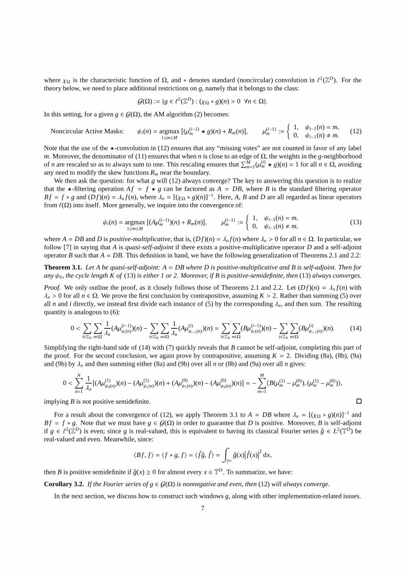
Corollary 3.2. If the Fourier series of g∈ G(Ω) is nonnegative and even, then(12) will always converge.

In the next section, we discuss how to construct such windowsg, along with other implementation-related issues.

7

4. Examples of Active Masks in practice

In this section we present a few representative and interesting examples of filter-based cellular automata, anddiscuss their behavior in relation with the results we proved in the previous sections. We also present some preliminaryexperimental findings on the rate of convergence of AM. For ease of understanding, let us for the moment restrictourselves to circulant iterative voting (1), namely the version of AM (2) in which all the skew functionsRm areidentically zero. The simplest nonzero filter isg = δ0. The DFT ofδ0 has constant value 1, and is therefore nonnegativeand even. As such, Theorem 1.1 guarantees that (1) will always converge. Of course, we already knew that: sincef ∗ δ0 = f for all f ∈ ℓ(Ω), (1) will always converge in one step; as noted above, the same holds true for anyg whoseconvolutional operator is strictly diagonally dominant with a nonnegative diagonal:g(0) ≥

∑

n,0 |g(n)|.More interesting examples arise frombox filters: symmetric cubes of Diracδ’s. For instance, fixN ≥ 3 and

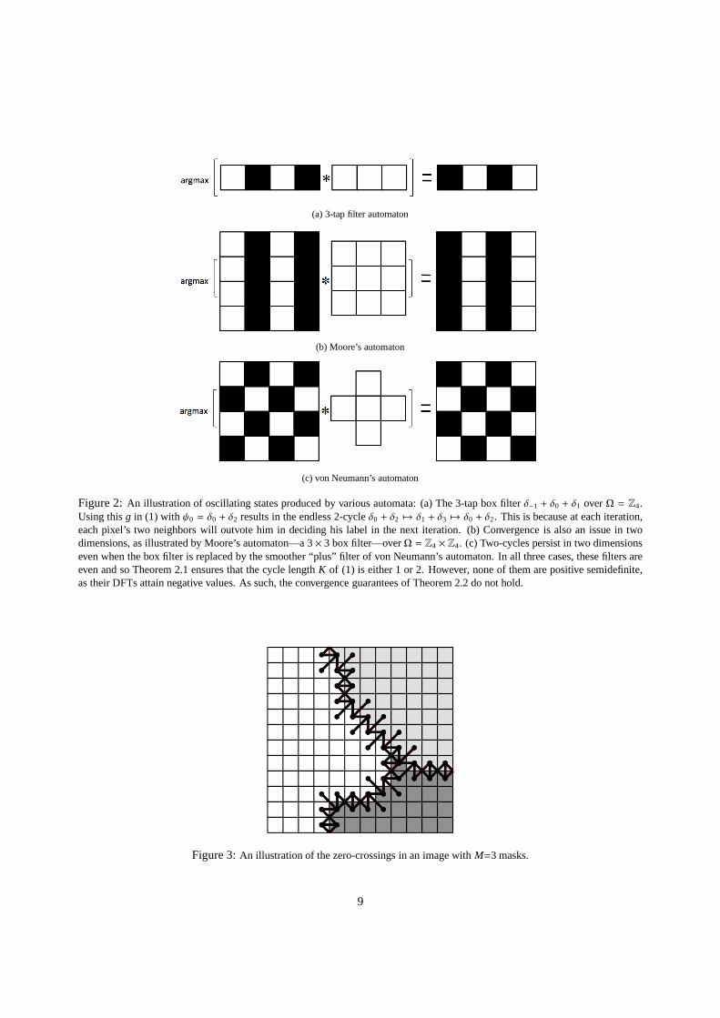
consider (1) overΩ = ZN whereg = δ−1 + δ0 + δ1. Sinceg is symmetric, Theorem 2.1 guarantees that (1) willeither always converge or will enter a 2-cycle. However, ifN is even, then (1) will not always converge, sinceψ0 = δ0+δ2+ · · ·+δN−2 generates a 2-cycle. This phenomenon is depicted in Figure 2(a). This simple example showsthat symmetry alone does not suffice to guarantee convergence; one truly needs additional hypotheses ong, such asthe requirement in Theorem 1.1 that its DFT is nonnegative. This hypothesis does not hold forg = δ−1 + δ0 + δ1,since (Fg)(n) = 1 + 2 cos(2πn

N ). Similar issues arise in the two-dimensional settingΩ = ZN1 × ZN2: both the 3× 3box filter (Moore’s automaton, see Figure 2(b)) and the “plus” filter (von Neumann’s automaton, see Figure 2(c))are symmetric, meaning their cycle lengths are either 1 or 2,but neither are positive semidefinite, having DFTs of[1 + 2 cos(2πn1

N1)][1 + 2 cos(2πn2

N2)] and 1+ 2 cos(2πn1

N1) + 2 cos(2πn2

N2), respectively. Indeed, whenN1 andN2 are even,

alternating stripes generate a 2-cycle for the box filter, while the checkerboard generates a 2-cycle for the plus filter.Of course, it is not difficult to find filtersg which do satisfy the hypotheses of Theorem 1.1: one may simply let

g be the inverse DFT of any nonnegative even function. More concrete examples, such as a discrete Gaussian overZN, can be found using the following process. Leth : R→ R be an even Schwartz function whose Fourier transformis nonnegative; an example of such a function is a continuousGaussian. Letg be theN-periodization of the integersamples ofh, namelyg(n) :=

∑∞n′=−∞ h(n+ Nn′). Theng is even, and moreover, by the Poisson summation formula:

(Fg)(n) =N−1∑

n′=0

g(n′)e−2πinn′

N =

N−1∑

n′=0

∞∑

n′′=−∞

h(n′ + Nn′′)e−2πinn′

N =

∞∑

k=−∞

h(k)e−2πink

N =

∞∑

k=−∞

h(k+ nN ) ≥ 0.

In particular, ifg is chosen as a periodized version of the integer samples of any zero-mean Gaussian, then Theorem 1.1gives that the AM algorithm (2) necessarily converges. Thisconstruction method immediately generalizes to higher-dimensional settings whereD > 1. It also generalizes to the noncircular convolution setting considered in Section 3.There, we further restricth to be strictly positive, and letg be the integer samples ofh. The positivity ofh implies(χΩ ∗ g)(n) > 0 for all n ∈ Ω, implying g ∈ G(Ω) as needed. Moreover,g is even and the Poisson summation formulagives that its Fourier series is nonnegative: ˆg(x) =

∑∞k=−∞ h(k+ x) ≥ 0. Any g constructed in this manner satisfies the

hypotheses of Corollary 3.2, implying the corresponding noncirculant AM (12) necessarily converges.

4.1. The rate of convergence of the AM algorithm

Up to this point, we have focused on the question of whether ornot the AM algorithm (2) converges. Havingsettled that question to some degree, our focus now turns to another question of primary importance in real-worldimplementation: at what rate does AM converge? Experimentation reveals that this rate highly depends on the con-figuration of the boundary between two distinctly labeled regions ofΩ. This led us to postulate that the numberof boundary crossings(see Figure 3) should monotonically decrease with each iteration. Experimentation revealsthat this number indeed often decreases extremely rapidly,regardless of the scale ofg. Figure 4 depicts such anexperiment for the fluorescence microscope image shown in Figure 1(a). Starting from a random initial configura-tion of 64 masks, we used a Gaussian filter under three different scales, with each plot depicting the evolution of 5independently-initialized runs of the algorithm. We emphasize the algorithm’s fast rate of convergence: the verticalaxis represents a nested four-fold application of the natural logarithm to the number of boundary crossings. We leavea more rigorous investigation of the AM algorithm’s rate of convergence for future work.

8

(a) 3-tap filter automaton

(b) Moore’s automaton

(c) von Neumann’s automaton

Figure 2:An illustration of oscillating states produced by various automata: (a) The 3-tap box filterδ−1 + δ0 + δ1 overΩ = Z4.Using thisg in (1) with ψ0 = δ0 + δ2 results in the endless 2-cycleδ0 + δ2 7→ δ1 + δ3 7→ δ0 + δ2. This is because at each iteration,each pixel’s two neighbors will outvote him in deciding his label in the next iteration. (b) Convergence is also an issue in twodimensions, as illustrated by Moore’s automaton—a 3× 3 box filter—overΩ = Z4 × Z4. (c) Two-cycles persist in two dimensionseven when the box filter is replaced by the smoother “plus” filter of von Neumann’s automaton. In all three cases, these filters areeven and so Theorem 2.1 ensures that the cycle lengthK of (1) is either 1 or 2. However, none of them are positive semidefinite,as their DFTs attain negative values. As such, the convergence guarantees of Theorem 2.2 do not hold.

Figure 3:An illustration of the zero-crossings in an image withM=3 masks.

9

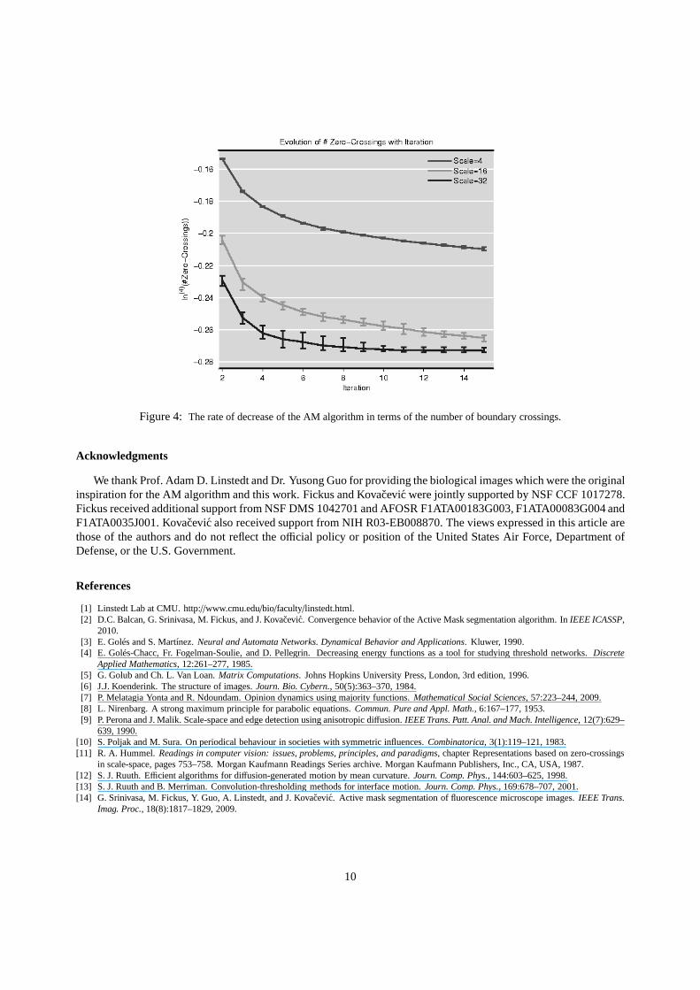
Figure 4: The rate of decrease of the AM algorithm in terms of the numberof boundary crossings.

Acknowledgments

We thank Prof. Adam D. Linstedt and Dr. Yusong Guo for providing the biological images which were the originalinspiration for the AM algorithm and this work. Fickus and Kovacevic were jointly supported by NSF CCF 1017278.Fickus received additional support from NSF DMS 1042701 andAFOSR F1ATA00183G003, F1ATA00083G004 andF1ATA0035J001. Kovacevic also received support from NIH R03-EB008870. The views expressed in this article arethose of the authors and do not reflect the official policy or position of the United States Air Force, Department ofDefense, or the U.S. Government.

References

[1] Linstedt Lab at CMU. http://www.cmu.edu/bio/faculty/linstedt.html.[2] D.C. Balcan, G. Srinivasa, M. Fickus, and J. Kovacevic. Convergence behavior of the Active Mask segmentation algorithm. InIEEE ICASSP,

2010.[3] E. Golés and S. Martínez.Neural and Automata Networks. Dynamical Behavior and Applications. Kluwer, 1990.[4] E. Golés-Chacc, Fr. Fogelman-Soulie, and D. Pellegrin.Decreasing energy functions as a tool for studying threshold networks. Discrete

Applied Mathematics, 12:261–277, 1985.[5] G. Golub and Ch. L. Van Loan.Matrix Computations. Johns Hopkins University Press, London, 3rd edition, 1996.[6] J.J. Koenderink. The structure of images.Journ. Bio. Cybern., 50(5):363–370, 1984.[7] P. Melatagia Yonta and R. Ndoundam. Opinion dynamics using majority functions.Mathematical Social Sciences, 57:223–244, 2009.[8] L. Nirenbarg. A strong maximum principle for parabolic equations.Commun. Pure and Appl. Math., 6:167–177, 1953.[9] P. Perona and J. Malik. Scale-space and edge detection using anisotropic diffusion.IEEE Trans. Patt. Anal. and Mach. Intelligence, 12(7):629–

639, 1990.[10] S. Poljak and M. Sura. On periodical behaviour in societies with symmetric influences.Combinatorica, 3(1):119–121, 1983.[11] R. A. Hummel.Readings in computer vision: issues, problems, principles, and paradigms, chapter Representations based on zero-crossings

in scale-space, pages 753–758. Morgan Kaufmann Readings Series archive. Morgan Kaufmann Publishers, Inc., CA, USA, 1987.[12] S. J. Ruuth. Efficient algorithms for diffusion-generated motion by mean curvature.Journ. Comp. Phys., 144:603–625, 1998.[13] S. J. Ruuth and B. Merriman. Convolution-thresholdingmethods for interface motion.Journ. Comp. Phys., 169:678–707, 2001.[14] G. Srinivasa, M. Fickus, Y. Guo, A. Linstedt, and J. Kovacevic. Active mask segmentation of fluorescence microscope images. IEEE Trans.

Imag. Proc., 18(8):1817–1829, 2009.

10