Gt Power

Tutorial: GT-Power Coupling

Purpose

The tutorial illustrates how to set up and solve a coupled simulation with GT-Power.

About GT-Power

GT-Power is a 1D engine simulation tool developed by Gamma Technologies Inc. (GTI),which has models for various components in the engine system, including intake, exhaust,turbochargers, EGR, catalytic converters etc. Tools such as GT-Power are valuable for per-forming parametric studies for the complete engine system because 1D models are relativelyinexpensive compared to multi-dimensional models.

However, some flow features are 3D in nature and are better analyzed using CFD. FLUENT/GT-Power coupling allows a component in the 1D system model to be replaced with a 3D CFDmodel.

GT-Power system models are set up and postprocessed in GT-ISE (Interactive SimulationEnvironment) developed by GTI. GT-ISE is a menu-driven, graphical user environment tobe used with GT-Power and other GTI engineering software. You can modify GT-Powervariables using GT-ISE, or by manually editing the GT-Power data file with any text editor.This tutorial does not cover the use of GTI software. Hence modifications to the GT-Powermodel will be made using the latter approach.

Boundary conditions are passed between the two codes in a coupled manner, eliminatingthe need for the user to specify these in the CFD model. Since the boundary conditionspassed to FLUENT include the effects of the attached system, the boundary treatment ismore accurate than stand-alone CFD simulation.

Prerequisites

This tutorial assumes that you are familiar with the menu structure in FLUENT, and withGT-Power, including specification of a CFD component. This tutorial will not cover GT-Power model setup.

For information on setting up boundary conditions with GT-Power, refer to section 7.29 ofFLUENT 6.2 User’s Guide.

Please refer to GT-Power documentation for details.

c© Fluent Inc. April 15, 2005 1

http://www.fluentusers.com/fluent/doc/ori/html/ug/node274.htm

http://www.fluentusers.com/fluent/doc/ori/html/ug/main_pre.htm


Problem Description

In this tutorial, the CFD domain consists of an intake manifold with an exhaust gas re-circulation (EGR) inlet. The GT-Power model contains a 4-cylinder engine with an EGRcircuit. EGR analysis is a good example for CFD analysis, as the flow is highly transientand 3D.

Preparation

1. FLUENT/GT-Power coupling requires installation of the appropriate GT-Power li-braries for your platform. This tutorial does not cover the installation procedureand assumes that the necessary GT-Power libraries have been installed on your sys-tem. These libraries are supplied by Fluent and they are available at Fluent UserServices Center. Furthermore, FLUENT/GT-Power coupling requires access to a validGT-Power license key. If you do not already have a valid GT-Power license key, contactGTI sales for assistance.

Note: FLUENT/GT-Power coupling is not available on all platforms. Please contactFLUENT or GTI technical support for a list of supported platforms.

2. Copy the mesh file, 4cyl-3d.msh.gz and the GT-Power input file, 4cyl-1d.dat toyour working directory.

3. Start the 3D version of FLUENT.

Setup and Solution

Step 1: Grid

1. Read the grid file (4cyl-3d.msh.gz).

File −→ Read −→Case...

2. Check the grid.

Grid −→Check

FLUENT will perform various checks on the mesh and will report the progress in theconsole window. Pay particular attention to the reported minimum volume. Makesure this is a positive number.

3. Change the reporting units of length for the grid.

Grid −→Scale...

2 c© Fluent Inc. April 15, 2005

http://www.fluentusers.com

http://www.fluentusers.com


(a) In the Units Conversion drop-down list, select mm to complete the phrase GridWas Created In mm (millimeters).

(b) Click on Change Length Units.

The final Domain Extents should appear as in the panel above.

! Do not scale the grid. The grid is scaled correctly. Length units are changedbecause it is more convenient to work in millimetres.

4. Display the grid (Figure 1).

Display −→Grid...

(a) In the Surfaces list, select all surfaces except default-interior.

(b) Click Display.

The boundaries with the prefixes inlet and outlet are the boundaries that will be coupledto the GT-Power model.

Use the right mouse button to check which zone number corresponds to each bound-ary. When you click the right mouse button on one of the boundaries in the graphicswindow, its zone number, name, and type will be displayed in the FLUENT consolewindow.

Step 2: Models

1. Define the solver settings.

Define −→ Models −→Solver...

(a) Under Time, select Unsteady.

Coupled GT-Power simulations in FLUENT require transient simulation.



outlet-cyl-4

outlet-cyl-3outlet-cyl-2

inlet-air

outlet-cyl-1

inlet-egr

Z

Y

X

GridFLUENT 6.2 (3d, segregated, lam)

Jan 14, 2005

Figure 1: Grid in the 4-cylinder Engine with EGR Circuit

2. Enable the k-ε turbulence model with standard wall functions.

Define −→ Models −→Viscous...

(a) Select k-epsilon (2 eqn) under Model.

(b) Accept all the default settings and click OK.

3. Specify the ideal-gas law for air (the default fluid material).

Define −→Materials...

(a) Select ideal-gas in the drop-down list for Density.

Note: When you select ideal-gas law, FLUENT automatically enables the energycalculation. So you need not open the Energy panel.

(b) Click the Change/Create button to save your changes.

4. Activate multiple species.

Define −→ Models −→ Species −→Transport & Reaction...

(a) Select Species Transport under Model.

(b) Retain all the default settings.

FLUENT will display an Information dialog box telling you that additional prop-erties have been defined for the new species. You will be setting properties in asubsequent step, so click OK to acknowledge this information.

You will modify the default mixture template in a later step to match the speciesreported in the GT-Power model.



Step 3: Materials

The fluid material type is used to specify properties of individual species, while the mixturematerial type is used to specify groupings of individual species. Properties of a mixturemay be defined to be composition dependent or composition independent. For compositiondependent mixture properties, the properties are specified for individual species, while forcomposition independent mixture properties, these are specified directly for the mixture.Species and mixture properties may be temperature dependent.

Material property specification is different in FLUENT and GT-Power. If there are significanttemperature variations in the CFD domain, it is advisable to modify the material propertiesappropriately as functions of temperature to be consistent with the GT-Power model.

1. Create individual material species to match those reported from GT-Power.

Define −→Materials...

(a) Select fluid in the drop-down list under Material Type.

(b) Define species, n2-vapc.

i. Select air in the drop-down list under Fluid Materials.

ii. Type n2-vapc in both the Name and Chemical Formula text entry boxes.

The species reported by GT-Power need to be matched with entries in theChemical Formula box.

iii. Click Change/Create to create the new species.

A question dialog box will appear, asking you if air should be overwritten.Click No to retain air and add the new material, n2-vapc, to the list. TheMaterials panel will be updated to show the new material name in the FluidMaterials list.

(c) Similarly, define o2-vapc, vap-indol, indolene-liqi, and burned.

It is possible to specify different molecular weights for each of the species but it issufficient to use the same molecular weight for all species since average molecularweight of the mixture does not vary significantly.

2. Create a mixture containing the species reported by GT-Power.

(a) In the Materials panel, select mixture in the Material Type drop-down list.

(b) Click on the Edit... button to the right of Mixture Species drop-down list in theProperties sub-window.

The list of species under Selected Species includes those species selected for thecurrent Mixture, while Available Materials includes all other species defined inthe current FLUENT session. The current listing of Selected Species reflectsthe default mixture-template. We will modify these species to match the mixturereported by GT-Power.

i. Select n2-vapc from the list of Available Materials and click Add.

This will move n2-vapc from the list of Available Materials to the bottom ofthe Selected Species list.



ii. Repeat the preceding step to add o2-vapc, vap-indol, indolene-liqi, and burnedto the list of Selected Species.

For N species in a mixture, FLUENT solves transport equations for N-1species mass fractions since the sum of species mass fractions must equal one,the Nth species mass fraction is determined algebraically. The last speciesin the list of Selected Species is not solved directly by a transport equation.Since adding always places the species to the Selected Species list, and thisallows you to control which species transport equations are to be solved.

iii. Remove the existing species h2o, o2, and n2. Select them individually andclick Remove.

iv. Click OK to apply the mixture definition.

(c) Select ideal-gas in the drop-down list for Density.

Select ideal gas law to resolve wave dynamics properly. Do not select the incompressible-ideal gas law or any other density specification method.

(d) Select piecewise-linear in the drop-down list for specific heat, Cp.



It is possible to define the specific heat of the mixture to be a function of indi-vidual species mass fractions using the mixing law option. But you can specifytemperature dependent specific heat for the mixture directly as a function of tem-perature, independent of the compositional makeup. This is a valid approximationif the mixture properties vary with temperature, but are not strongly affected bycomposition.

i. Increase the number of Points to 5.

ii. Under Data Points, specify the values as shown in the table:

Point Temperature (k) Value (j/kg-k)

1 300 10052 500 10303 700 10754 900 11235 1100 1161

(e) Click Change/Create in the Materials panel to apply the property modifications.

(f) Close the Materials panel.

Step 4: Importing the GT-Power Input File

1. Specify the GT-Power input file.

Define −→ User-Defined −→1D Coupling...

(a) Keep the default selection of GTpower in the 1D Library drop-down list.

(b) Specify 4cyl-1d.dat for 1D Input File Name.

This is a GT-Power data file (not a FLUENT data file) which contains the 1Dsystem model information. Be careful not to confuse FLUENT .dat files andGT-Power .dat files, as the data files of each have the same file extension. In thecurrent tutorial, the FLUENT case and data files are named 4cyl-3d.cas and4cyl-3d.dat, and the GT-Power data file is called 4cyl-1d.dat.

(c) Click Start to open the GT-Power library.

If the GT-Power link is established successfully, GT-Power output will be reportedin the FLUENT console.



Step 5: Operating Conditions

Define −→Operating Conditions...

1. Under Operating Pressure, enter 200000 pascal.

The GT-Power model is set up with a high pressure in the intake system to representa turbocharged or supercharged engine.

2. Click OK.

Step 6: Boundary Conditions

For each coupled boundary zone in FLUENT, the GT-Power data file must contain a corre-sponding CFDConnection object. Each CFDConnection object includes information identify-ing this object (Part Name in GT-Power) and the boundary type to be used in FLUENT. Whenthe GT-Power library is opened, the CFDConnection identification and boundary type infor-mation is passed to FLUENT for each coupled boundary specified in the GT-Power data file.In FLUENT, each coupled boundary zone must be matched with the corresponding GT-PowerPart Name identifier.

GT-Power allows specification of two boundary types, inlet and pressure. To use a mass-flow inlet boundary condition in FLUENT, you must specify inlet type for the correspondingCFDConnection, and if you wish to choose a pressure boundary condition in FLUENT, specifythe pressure type.

In this, six CFDConnection objects are defined in the 4cyl-1d.dat GT-Power data file. Parts103, 13, 105, 106, 107, and 108 correspond to inlet-air, inlet-egr, outlet-cyl-1, outlet-cyl-2,outlet-cyl-3, and outlet-cyl-4, respectively. All these boundaries are specified as inlet typeboundaries in the GT-Power data file.

Define −→Boundary Conditions

1. Apply boundary conditions for the fresh-air inlet.

(a) Select inlet-air from the Zone list and click Set....



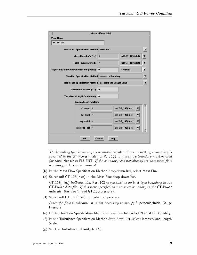
The boundary type is already set as mass-flow inlet. Since an inlet type boundary isspecified in the GT-Power model for Part 103, a mass-flow boundary must be usedfor zone inlet-air in FLUENT. If the boundary was not already set as a mass-flowboundary, it has to be changed.

(b) In the Mass Flow Specification Method drop-down list, select Mass Flux.

(c) Select udf GT 103(inlet) in the Mass Flux drop-down list.

GT 103(inlet) indicates that Part 103 is specified as an inlet type boundary in theGT-Power data file. If this were specified as a pressure boundary in the GT-Powerdata file, this would read GT 103(pressure).

(d) Select udf GT 103(inlet) for Total Temperature.

Since the flow is subsonic, it is not necessary to specify Supersonic/Initial GaugePressure.

(e) In the Direction Specification Method drop-down list, select Normal to Boundary.

(f) In the Turbulence Specification Method drop-down list, select Intensity and LengthScale.

(g) Set the Turbulence Intensity to 5%.



(h) Set the Turbulence Length Scale to 6 mm.

(i) Under Species Mass Fractions, select udf GT 103(inlet) in the n2-vapc drop-downlist.

(j) Select udf GT 103(inlet) for o2-vapc.

(k) Select udf GT 103(inlet) for vap-indol.

(l) Select udf GT 103(inlet) for indolene-liqi.

Note: There is no entry for species burned since this is the final selected species.With knowledge of all other species, burned is determined so that all speciesmass fractions add up to 1.

(m) Click OK to apply the boundary condition settings.

2. Apply boundary conditions to the EGR inlet.

(a) Select inlet-egr from the Zone list and click Set....


(c) Select udf GT 13(inlet) for both Mass Flux and Total Temperature.

(d) In the Direction Specification Method drop-down list, select Normal to Boundary.

(e) In the Turbulence Specification Method drop-down list, select Intensity and LengthScale.

(f) Set the Turbulence Intensity to 5%.

(g) Set the Turbulence Length Scale to 3.2 mm.

(h) Under Species Mass Fractions, select udf GT 13(inlet) in the n2-vapc drop-downlist.

(i) Select udf GT 13(inlet) for o2-vapc, vap-indol, and indolene-liqi.

(j) Click OK to apply the boundary condition settings.

3. Apply boundary conditions to outlet-cyl1, the first intake manifold runner exit.

(a) Select outlet-cyl-1 from the Zone list and click Set....


(c) Select udf GT 105(inlet) for Mass Flux and Total Temperature.

(d) In the Direction Specification Method drop-down list, select Normal to Boundary.

(e) In the Turbulence Specification Method drop-down list, select Intensity and LengthScale.

(f) Set the Turbulence Intensity to 5%.

(g) Set the Turbulence Length Scale to 3.5 mm.

(h) Under Species Mass Fractions, select udf GT 105(inlet) in the n2-vapc drop-downlist.

(i) Select udf GT 105(inlet) for o2-vapc, vap-indol, and indolene-liqi.

(j) Click OK to apply the boundary condition settings.



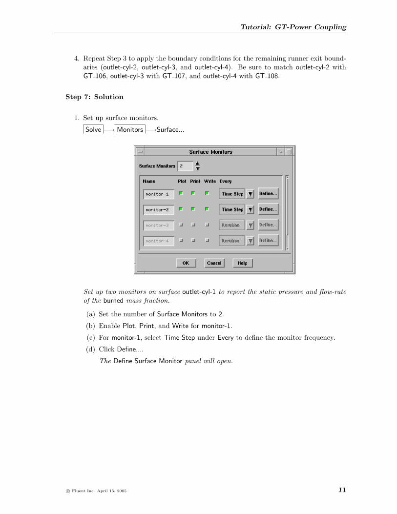
4. Repeat Step 3 to apply the boundary conditions for the remaining runner exit bound-aries (outlet-cyl-2, outlet-cyl-3, and outlet-cyl-4). Be sure to match outlet-cyl-2 withGT 106, outlet-cyl-3 with GT 107, and outlet-cyl-4 with GT 108.

Step 7: Solution

1. Set up surface monitors.

Solve −→ Monitors −→Surface...

Set up two monitors on surface outlet-cyl-1 to report the static pressure and flow-rateof the burned mass fraction.

(a) Set the number of Surface Monitors to 2.

(b) Enable Plot, Print, and Write for monitor-1.

(c) For monitor-1, select Time Step under Every to define the monitor frequency.

(d) Click Define....

The Define Surface Monitor panel will open.



i. Select Flow Time in the drop-down list under X-Axis.

ii. Select Pressure... and Static Pressure in the Report Of drop-down lists.

iii. Select outlet-cyl-1 under Surfaces.

iv. Enter monitor-1.out under the File Name text-entry box.

v. Click OK to enter the information for the first monitor.

(e) In the Surface Monitors panel, enable Plot, Print, and Write for monitor-2.

(f) In the drop-down list to the right of monitor-2, select Time Step for the monitorfrequency.

(g) Click Define....

i. In the Define Surface Monitor panel, select Flow Time in the drop-down listunder X-Axis.

ii. Select Species... and Mass fraction of burned in the Report Of drop-down lists.

iii. Select outlet-cyl-1 under Surfaces.

iv. Enter monitor-2.out under the File Name text-entry box.

v. Click OK to enter the information for the second monitor.

(h) Click OK in the Surface Monitors panel.

2. Set up residual monitors.

Solve −→ Monitors −→Residual...

(a) Select the Plot option.

(b) Close the residual monitor panel.



3. Initialize the solution.

Solve −→ Initialize −→Initialize...

Initialize the solution at this point so that you can display contours to set up the viewfor the animation. To reduce the number of cycles to attain a periodic solution, initial-ize the flow with a representative mixture in the manifold. Set the initial compositionin the manifold to contain a mixture of 0.9 mass fraction of air (23.3% oxygen and76.7% nitrogen) and 0.1 mass fraction of burned.

(a) Set the Gauge Pressure to 0 pascal.

(b) Set X Velocity, Y Velocity, and Z Velocity to 0 m/s.

(c) Set Turbulence Kinetic Energy to 1 m2/s2.

(d) Set Turbulence Dissipation Rate to 1 m2/s3.

(e) Set n2-vapc Mass Fraction to 0.6903.

(f) Set o2-vapc Mass Fraction to 0.2097.

(g) Set vap-indol Mass Fraction to 0.

(h) Set indolene-liqi Mass Fraction to 0.

(i) Set initial Temperature to 300 k.

(j) Click Apply.

The Apply button does not initialize the flow field data. It allows you to storeyour initialization parameters for later use. You must use the Init button.

(k) Click Init to initialize the flow and close the panel.

4. Set up an animation.

(a) Display contours.

Display −→Contours...

i. Select Species... and Mass Fraction of burned in the Contour Of drop-downlist.

ii. Under Surfaces, select all surfaces except default-interior.

iii. Select Filled under Options.

iv. Click Display.

Arrange the view so that the entire domain will fit into the display.

v. Close the Contours panel.

(b) Save the view.

Display −→Views...

i. Under Actions, click the Save button to save view-0.

ii. Close the Views panel.

(c) Open the command monitor window.

Solve −→Execute Commands...



i. Set Defined Commands to 1.

ii. Select the checkbox under the On column.

iii. Set 5 as the value under the Every column.

iv. Select Time Step in the drop-down list under When.

v. In the Command text-entry box, type in:

/display/set-window 3 /display/view/restore-view view-0

/display/contour burned 0 0.3 /display/hardcopy burned%t.tiff

This should be entered as a single line. This will first set window 3 as theactive window, restore view-0, display contours of the burned species scaledfrom 0.0 to 0.3, and then make a hardcopy of the resulting image. The %tappended to the filename instructs FLUENT to append the time step index tothe filename. It is also possible to specify multiple text commands as a singleentry.

vi. Click OK.

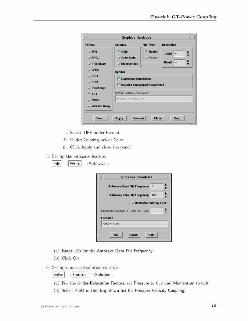
(d) Set hardcopy settings.

File −→Hardcopy...



i. Select TIFF under Format.

ii. Under Coloring, select Color.

iii. Click Apply and close the panel.

5. Set up the autosave feature.

File −→ Write −→Autosave...

(a) Enter 180 for the Autosave Data File Frequency.

(b) Click OK.

6. Set up numerical solution controls.

Solve −→ Control −→Solution...

(a) For the Under-Relaxation Factors, set Pressure to 0.7 and Momentum to 0.9.

(b) Select PISO in the drop-down list for Pressure-Velocity Coupling.



(c) Set the values of Skewness Correction and Neighbor Correction to zero.

(d) Deselect Skewness-Neighbor Coupling and click OK to apply the settings.

7. Set the time stepping parameters.

Solve −→Iterate...

In the GT-Power model, a parameter called DURATN controls the number of total cyclesto be run before GT-Power specific output files are written (these include *.gb and*.rlt files). For FLUENT/GT-Power coupled simulations, an additional parametercalled TLAG is used to set the number of “pre-cycles”. During the pre-cycles, GT-Powerruns independently from FLUENT and uses a simple zero-dimensional representationof the CFD component. This allows the GT-Power system model to stabilize before thecoupling begins. In the current tutorial, 13 total cycles with 10 pre-cycles are specifiedin the GT-Power .dat file. This results in three coupled cycles.

(a) Specify a Time Step Size of 2.873563e-5 s.

This time step corresponds to 1 degree crank angle at 5800 rpm. Apply will savethe time step in the case file when the case is saved.

(b) Click Apply.

8. Save the case file (4cyl-3d.cas.gz).

File −→ Write −→Case...

9. Run the calculation.

(a) Enter 2170 for the Number of Time Steps.

2170 time steps is slightly greater than three crank revolutions, and will ensurethat the GT-Power output files are updated at the end of the third coupled cycle.

(b) Click Iterate.

Step 8: Postprocessing

1. Display filled contours of pressure (Figure 2).


(a) Select Filled under Options.

(b) Select Pressure... and Static Pressure in the Contours Of drop-down lists.

(c) Click Display.

2. Display filled contours of temperature (Figure 3).

3. Display the mass fraction for n2-vapc (Figure 4).

(a) Select Species... and Mass fraction of n2-vapc in the Contours Of drop-down lists.

(b) Click Display.

4. Select other species and display their mass fraction distribution (Figures 5–8).



Contours of Static Pressure (pascal) (Time=6.2069e-02)FLUENT 6.2 (3d, segregated, spe, ske, unsteady)

Feb 14, 2005

3.16e+042.79e+042.43e+042.07e+041.70e+041.34e+049.76e+036.13e+032.49e+03-1.14e+03-4.77e+03-8.40e+03-1.20e+04-1.57e+04-1.93e+04-2.29e+04-2.66e+04-3.02e+04-3.38e+04-3.75e+04-4.11e+04

Z

Y

X

Figure 2: Contours of Pressure for the 4-cylinder engine with EGR circuit

Contours of Static Temperature (k) (Time=6.2069e-02)FLUENT 6.2 (3d, segregated, spe, ske, unsteady)

Feb 14, 2005

9.69e+029.36e+029.02e+028.69e+028.36e+028.02e+027.69e+027.35e+027.02e+026.68e+026.35e+026.02e+025.68e+025.35e+025.01e+024.68e+024.35e+024.01e+023.68e+023.34e+023.01e+02

Z

Y

X

Figure 3: Contours of Temperature for the 4-cylinder engine with EGR circuit



Contours of Mass fraction of n2-vapc (Time=6.2069e-02)FLUENT 6.2 (3d, segregated, spe, ske, unsteady)

Feb 14, 2005

7.67e-017.29e-016.90e-016.52e-016.14e-015.75e-015.37e-014.99e-014.60e-014.22e-013.84e-013.45e-013.07e-012.68e-012.30e-011.92e-011.53e-011.15e-017.67e-023.84e-020.00e+00

Z

Y

X

Figure 4: Contours of Mass Fraction of n2-vapc

Contours of Mass fraction of o2-vapc (Time=6.2069e-02)FLUENT 6.2 (3d, segregated, spe, ske, unsteady)

Feb 14, 2005


Z

Y

X

Figure 5: Contours of Mass Fraction of o2-vapc



Contours of Mass fraction of vap-indol (Time=6.2069e-02)FLUENT 6.2 (3d, segregated, spe, ske, unsteady)

Feb 14, 2005


Z

Y

X

Figure 6: Contours of Mass Fraction of vap-indol

Contours of Mass fraction of indolene-liqi (Time=6.2069e-02)FLUENT 6.2 (3d, segregated, spe, ske, unsteady)

Feb 14, 2005


Z

Y

X

Figure 7: Contours of Mass Fraction of indolene-liqi



Contours of Mass fraction of burned (Time=6.2069e-02)FLUENT 6.2 (3d, segregated, spe, ske, unsteady)

Feb 14, 2005

1.00e-009.50e-019.00e-018.50e-018.00e-017.50e-017.00e-016.50e-016.00e-015.50e-015.00e-014.50e-014.00e-013.50e-013.00e-012.50e-012.00e-011.50e-011.00e-015.00e-023.73e-09

Z

Y

X

Figure 8: Contours of Mass Fraction of burned

5. Display velocity vectors (Figure 9).

Display −→Vectors...

(a) Select Velocity... and Velocity Magnitude in the Color By drop-down lists.

(b) Click Display.



Velocity Vectors Colored By Velocity Magnitude (m/s) (Time=6.2069e-02)FLUENT 6.2 (3d, segregated, spe, ske, unsteady)

Feb 14, 2005

1.76e+021.67e+021.58e+021.49e+021.41e+021.32e+021.23e+021.14e+021.05e+029.67e+018.80e+017.92e+017.05e+016.17e+015.29e+014.42e+013.54e+012.67e+011.79e+019.14e+003.79e-01

Z

Y

X

Figure 9: Velocity Vectors Colored By Velocity Magnitude

Step 9: Restarting the Calculation from Saved Data

To restart the calculation from the saved data file, you need to edit the GT-Power data file.See Appendix for further details.

1. Exit the current FLUENT session.

File −→Exit...

FLUENT will display a Warning dialog box telling you that the current data has notbeen saved. Since the data was saved at time step 2160, it is not necessary to save thedata. Click OK to exit.

2. Edit the 4cyl-1d.dat file with any text editor.

In the event of an editing error, backup copies of the GT-Power data file are provided.These files are 4cyl-1d.dat.1 and 4cyl-1d.dat.2.

(a) Change the IRESTR variable from none to cfdreload.

(b) Change the ITERREST variable from ign to 2160.

Variable cfdreload indicates that the solution should be restarted from the savedfile. The number 2160 is the time step at which solution data is saved and fromwhere the calculation should be started

(c) Save the file with the same name.

Compare the modifications done to 4cyl-1d.dat with the 4cyl-1d.dat.2 file.On UNIX platforms, use the “diff” command (diff 4cyl-1d.dat 4cyl-1d.dat.2)to compare the file. On Windows systems, use the “fc” command in a commandwindow (fc 4cyl-1d.dat 4cyl-1d.dat.2).



3. Start the 3D version of FLUENT.

4. Read the FLUENT case file (4cyl-3d.cas.gz).

File −→ Read −→Case...

5. Read the corresponding FLUENT data file (4cyl-3d2160.dat.gz).

File −→ Read −→Data...

6. Resume the calculation for an additional 725 time steps.

Solve −→Iterate...

(a) Set the Number of Time Steps to 725.

(b) Click Iterate.

Step 10: Postprocessing (After 725 Iterations)

1. Display filled contours of pressure and temperature (Figures 10 and 11).


Contours of Static Pressure (pascal) (Time=8.2902e-02)FLUENT 6.2 (3d, segregated, spe, ske, unsteady)

Feb 14, 2005

2.13e+041.81e+041.50e+041.19e+048.76e+035.63e+032.51e+03-6.18e+02-3.74e+03-6.87e+03-9.99e+03-1.31e+04-1.62e+04-1.94e+04-2.25e+04-2.56e+04-2.87e+04-3.19e+04-3.50e+04-3.81e+04-4.12e+04

Z

Y

X

Figure 10: Contours of Pressure for the 4-cylinder engine with EGR circuit

2. Display the mass fraction for all species (Figures 12 – 16).

3. Display velocity vectors (Figure 17).

Display −→Vectors...



Contours of Static Temperature (k) (Time=8.2902e-02)FLUENT 6.2 (3d, segregated, spe, ske, unsteady)

Feb 14, 2005

9.61e+029.28e+028.95e+028.62e+028.29e+027.96e+027.63e+027.30e+026.97e+026.64e+026.31e+025.98e+025.65e+025.33e+025.00e+024.67e+024.34e+024.01e+023.68e+023.35e+023.02e+02

Z

Y

X

Figure 11: Contours of Temperature for the 4-cylinder engine with EGR circuit

Contours of Mass fraction of n2-vapc (Time=8.2902e-02)FLUENT 6.2 (3d, segregated, spe, ske, unsteady)

Feb 14, 2005


Z

Y

X

Figure 12: Contours of Mass Fraction of n2-vapc



Contours of Mass fraction of o2-vapc (Time=8.2902e-02)FLUENT 6.2 (3d, segregated, spe, ske, unsteady)

Feb 14, 2005


Z

Y

X

Figure 13: Contours of Mass Fraction of o2-vapc

Contours of Mass fraction of vap-indol (Time=8.2902e-02)FLUENT 6.2 (3d, segregated, spe, ske, unsteady)

Feb 14, 2005


Z

Y

X

Figure 14: Contours of Mass Fraction of vap-indol



Contours of Mass fraction of indolene-liqi (Time=8.2902e-02)FLUENT 6.2 (3d, segregated, spe, ske, unsteady)

Feb 14, 2005


Z

Y

X

Figure 15: Contours of Mass Fraction of indolene-liqi

Contours of Mass fraction of burned (Time=8.2902e-02)FLUENT 6.2 (3d, segregated, spe, ske, unsteady)

Feb 14, 2005


Z

Y

X

Figure 16: Contours of Mass Fraction of burned



Velocity Vectors Colored By Velocity Magnitude (m/s) (Time=8.2902e-02)FLUENT 6.2 (3d, segregated, spe, ske, unsteady)

Feb 14, 2005

1.90e+021.80e+021.71e+021.61e+021.52e+021.43e+021.33e+021.24e+021.14e+021.05e+029.51e+018.57e+017.62e+016.67e+015.72e+014.78e+013.83e+012.88e+011.93e+019.88e+004.02e-01

Z

Y

X

Figure 17: Velocity Vectors Colored By Velocity Magnitude

Summary

This tutorial demonstrated how to set up and solve a GT-Power simulation.



Appendix

Resuming a Simulation from the Saved Data File

It is often necessary to resume a simulation from a saved data file. To accomplish this, youneed to edit few variables in the GT-Power data file.

Restart specification is controlled by the IRESTR variable in the GT-Power data file. Spec-ifying this as None instructs GT-Power to start from initial conditions, while cfdreloadinstructs GT-Power to restart the calculation.

The time step from which the calculation should be restarted is controlled by the variable,ITERREST. Set the value of this variable to the time step (e.g., 2160 in this case) fromwhich you need to resume the calculation.

GT-Power writes the boundary value data for each time step in a .cfd file. While restartingthe simulation, GT-Power reads the boundary values upto that particular time step fromthe .cfd file and resumes the calculation.


Gt Power

Documents

power license key

velocity vectors colored

power input le

boundary condition settings

species mass fractions

power data le

saved data le

turbulence length scale