GSTARS Computer Models and Sedimentation Control in Surface Water

The 3rd International Conference on Water Resources and Arid Environments (2008) and the 1st Arab Water Forum

GSTARS Computer Models and Sedimentation Control in Surface Water Systems

Chih Ted Yang

Hydroscience and Training Center, Colorado State University, Fort Collins, Colorado, USA

Abstract

GSTARS (Generalized Sediment Transport model for Alluvial River Simulation) is a series of computer models developed by the U.S. Bureau of Reclamation while the author was employed by that agency. The stream tube concept is used in all GSTARS models which allow us to solve one-dimensional equations for each stream tube independently and obtain semi-two-dimensional variation of the hydraulic conditions along and across stream tubes for rivers and reservoirs. Sediment transport, scour, and deposition processes are simulated along each stream tube independently to give us a semi-three-dimensional variation of the bed geometry. Most sediment transport computer models assume that channel width is set (or static) and cannot change during the simulation process. GSTARS models apply the theory of minimum stream power for the determination of optimum channel width and channel geometry. The concepts of channel side stability, and active, inactive, and armoring layers are used in all GSTARS models for realistic long-term simulation and prediction of the scour and deposition processes in rivers and reservoirs. GSTARS models have been applied in many countries for solving a wide range of river and reservoir sedimentation problems. Case studies will be used to illustrate the application of GSTARS computer models for sedimentation control in surface water systems. Keywords: Computer model, Reservoir, River, Sediment transport

Introduction GSTARS is a series of computer models developed by the U.S. Bureau of

Reclamation for alluvial river and reservoir sedimentation studies while the author was employed by that agency. GSTARS stands for Generalized Stream Tube model for Alluvial River Simulation. The first version of GSTARS was released in 1986 (Molinas and Yang) using Fortran IV for mainframe computers. GSTARS 2.0 was released in 1998 (Yang, et al.) for PC application, with most of the programs in the original GSTARS revised, improved, and expanded using Fortran IV/77. GSTARS 2.1 (Yang and Simões, 2002) is an improved and revised GSTARS 2.0 with graphical interface to improve the program’s user friendliness. The unique features of all GSTARS models are the conjunctive use of stream tube concept and the minimum stream power theory. The use of stream tube concept enables us to simulate river hydraulics using one-dimensional numerical solutions to obtain a semi-two-dimensional presentation of the hydraulic conditions along and across an alluvial channel. The application of minimum stream power theory (Yang 1996, 1992; Yang and Song 1986, 1979; and Chang 1979, 1990) allows us to determine the optimum channel geometry with variable channel width and cross-sectional shape. According to the stream tube concept, no water or sediment particles can cross the walls of stream tubes; that concept is valid for most of the natural rivers. At and near a sharp bend, sediment particles may cross the boundaries of stream tubes due to their gravity while water still flows within the stream tube boundaries. GSTARS3 (Yang and Simões, 2002) recognizes this phenomenon and further expands the capabilities of GSTARS 2.1 for cohesive and non-cohesive sediment transport in rivers and reservoirs. In GSTARS3, bed load sediments are allowed to cross stream tube boundaries. Examples will be used to illustrate the applications of GSTARS models for the study of sedimentation control in surface water systems. Basic Requirements of a Generalized Model for Rivers and Reservoirs A generalized computer model for rivers and reservoirs should satisify the following requirements: (1). It should be able to compute hydraulic parameters for open channels with fixed as well as movable boundaries; (2). It should have the capability of computing water surface profiles in the subcritical, supercritical, and mixed flow regimes, i.e., in combinations of subcritical and supercritical flows without interruption; (3). It should be able to simulate and predict the hydraulic and sediment variations both in the longitudinal and in the transverse directions; (4). It should be able to simulate and predict the change of alluvial channel profile and cross-sectional geometry, regardless of whether the channel width is variable or fixed; (5). It should incorporate site specific conditions such as channel side stability and erosion limits; (6). It should be able to simulate and predict sediment transport by size fraction so

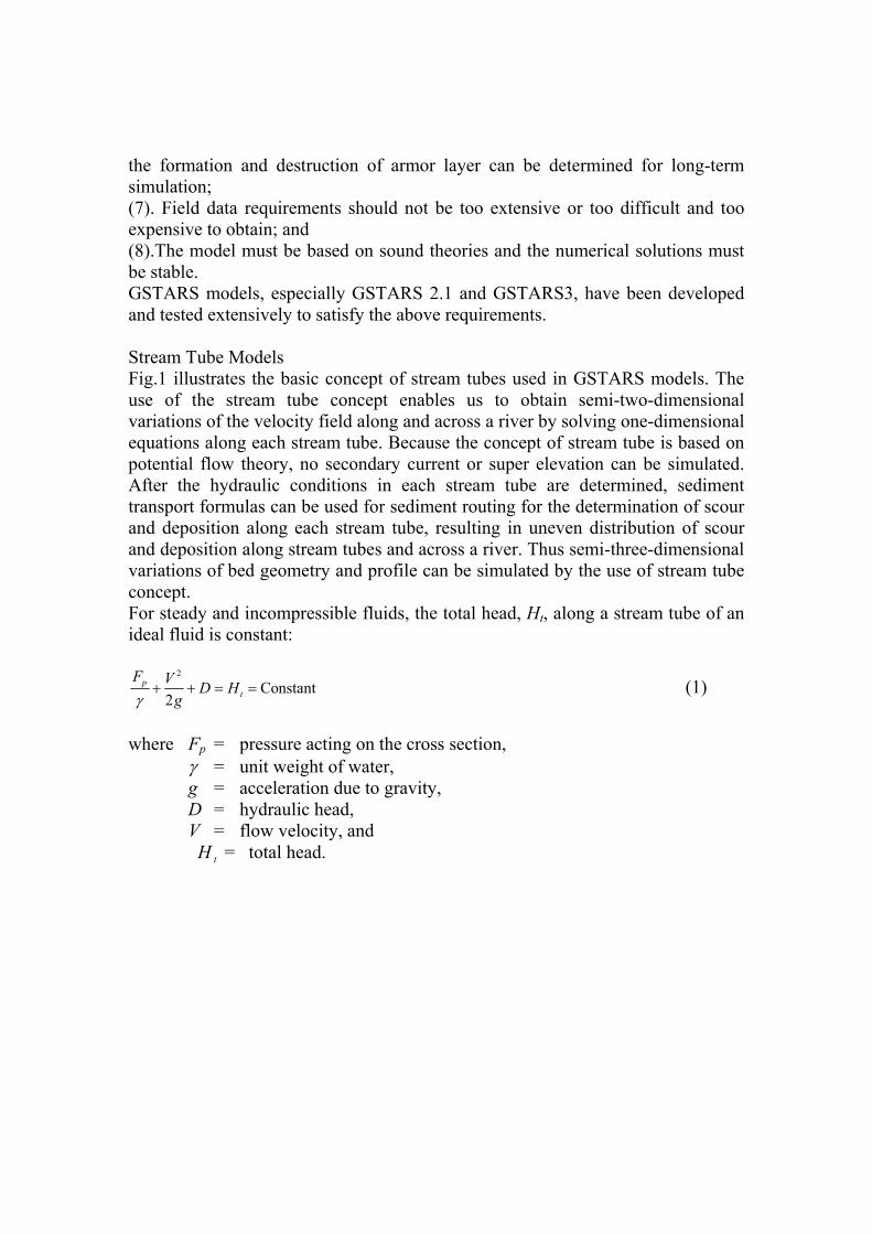
the formation and destruction of armor layer can be determined for long-term simulation; (7). Field data requirements should not be too extensive or too difficult and too expensive to obtain; and (8).The model must be based on sound theories and the numerical solutions must be stable. GSTARS models, especially GSTARS 2.1 and GSTARS3, have been developed and tested extensively to satisfy the above requirements. Stream Tube Models Fig.1 illustrates the basic concept of stream tubes used in GSTARS models. The use of the stream tube concept enables us to obtain semi-two-dimensional variations of the velocity field along and across a river by solving one-dimensional equations along each stream tube. Because the concept of stream tube is based on potential flow theory, no secondary current or super elevation can be simulated. After the hydraulic conditions in each stream tube are determined, sediment transport formulas can be used for sediment routing for the determination of scour and deposition along each stream tube, resulting in uneven distribution of scour and deposition along stream tubes and across a river. Thus semi-three-dimensional variations of bed geometry and profile can be simulated by the use of stream tube concept. For steady and incompressible fluids, the total head, Ht, along a stream tube of an ideal fluid is constant:

2

Constant2

pt

F V D Hgγ

+ + = = (1)

where Fp = pressure acting on the cross section, γ = unit weight of water, g = acceleration due to gravity, D = hydraulic head, V = flow velocity, and H t = total head.

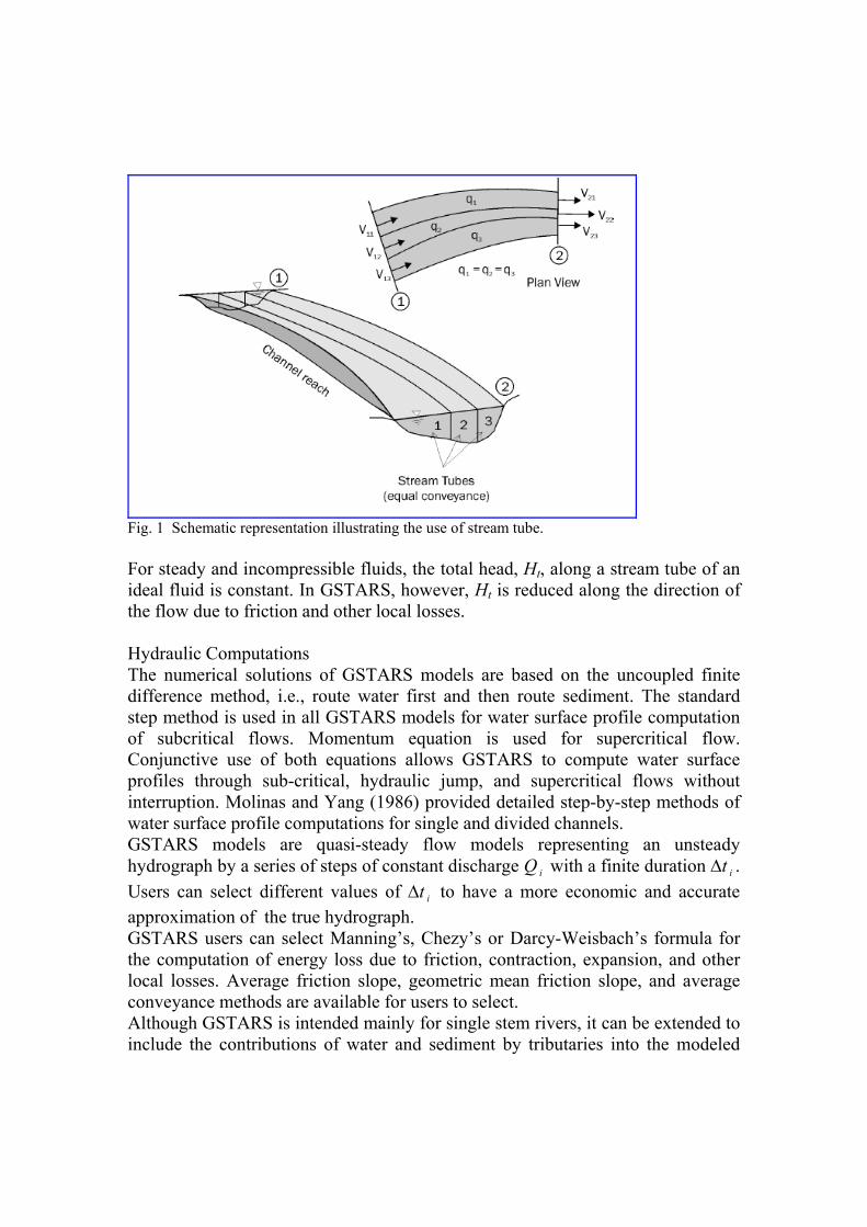
Fig. 1 Schematic representation illustrating the use of stream tube. For steady and incompressible fluids, the total head, Ht, along a stream tube of an ideal fluid is constant. In GSTARS, however, Ht is reduced along the direction of the flow due to friction and other local losses. Hydraulic Computations The numerical solutions of GSTARS models are based on the uncoupled finite difference method, i.e., route water first and then route sediment. The standard step method is used in all GSTARS models for water surface profile computation of subcritical flows. Momentum equation is used for supercritical flow. Conjunctive use of both equations allows GSTARS to compute water surface profiles through sub-critical, hydraulic jump, and supercritical flows without interruption. Molinas and Yang (1986) provided detailed step-by-step methods of water surface profile computations for single and divided channels. GSTARS models are quasi-steady flow models representing an unsteady hydrograph by a series of steps of constant discharge Q i with a finite duration ∆t i . Users can select different values of ∆t i to have a more economic and accurate approximation of the true hydrograph. GSTARS users can select Manning’s, Chezy’s or Darcy-Weisbach’s formula for the computation of energy loss due to friction, contraction, expansion, and other local losses. Average friction slope, geometric mean friction slope, and average conveyance methods are available for users to select. Although GSTARS is intended mainly for single stem rivers, it can be extended to include the contributions of water and sediment by tributaries into the modeled

reach. At channel junctions, continuity requires that bac QQQ += (2) where Q a , Q b , and Q c = water discharges of tributaries a and b, and main stem c,

respectively. Conservation of energy at the conference requires that

( fba hg

VYZg

VYZ +++=++ )2

()2

22

αα (3)

where h f = energy loss due to bends, contraction, and expansion at the confluence of the two tributaries. 5. Sediment Transport Computations GSTARS3 has the following transport functions for users to select: 1) DuBoy’s 1897 method (2) Meyer-Peter and Müller’s 1948 method (3) Laursen’s 1958 method (4) Modified Laursen’s method by Madden (1993) (5) Toffaleti’s 1969 method (6) Engelund and Hansen’s 1972 method (7) Ackers and White’s 1973 method (8) Revised Acker and White’s 1990 method (9) Yang’s 1973 sand and 1984 gravel transport methods (10) Yang’s 1979 and 1984 gravel transport methods (11) Parker’s 1990 method (12) Yang’s 1996 modified method for high concentration of wash load (13) Ashida and Michiue’s 1972 method (14) Tsinghua University method (IRTCES, 1985) (15) Krone’s (1962) and Ariathural and Krone’s (1976) methods for cohesive sediment transport. In addition to the above 17 commonly used methods, GSTARS 2.1 and GSTARS3 users can add additional methods to satisfy certain site specific conditions. Comparisons of commonly used sediment transport formulas made by the American Society of Civil Engineers (1982) and Alonso (1980), among others, were summarized by Yang (1996, 2003). GSTARS users should use the guidelines recommended by Yang (1996, 2003, 2006) as reference in the selection of appropriate formulas in the application of GSTARS models.

The above methods were developed mainly for fairly uniform sediments of a certain representative particle size. For graded sediments, the following equation should be used

( )[ ]i

N

iii prrpC ∑

=

−+=1

*1 iC (4)

where =ip percentage of material of size fraction i available in the bed, =*

ip percentage of material of size fraction i incoming into the study reach, =iC transport capacity for each size fraction computed by one of the sediment transport methods, r = a factor between 0 and 1, and N = number of size fractions. The basis for sediment routing computation for GSTARS models is the following conservation equation of sediment

0=−∂∂

+∂∂

+∂∂

latsds q

tA

tA

xQ

η (5)

where η = volume of sediment in a unit bed layer volume (one minus porosity), A d , sA = sediment volume in bed and in suspension, respectively, t = time, and q lat = lateral sediment inflow. If the change of suspended sediment concentration in a cross section is much smaller than the change of river bed,

0=∂∂

tQs , or

dxdQ

xQ sx =∂∂ (6)

and Equation (5) becomes

latsd q

dxdQ

tA

=+∂∂

η (7)

GSTARS3 includes the effects of stream curvature that contribute to the radial (transverse) flux of sediments, rq , near the bed. Fig. 2 illustrates bed sorting in bends due to transverse bed slope and secondary currents.

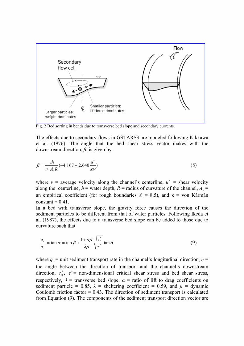
Fig. 2 Bed sorting in bends due to transverse bed slope and secondary currents. The effects due to secondary flows in GSTARS3 are modeled following Kikkawa et al. (1976). The angle that the bed shear stress vector makes with the downstream direction, β, is given by

)640.2167.4(*

* κνβ u

RAuvh

r

+−= (8)

where ν = average velocity along the channel’s centerline, u * = shear velocity along the centerline, h = water depth, R = radius of curvature of the channel, A r = an empirical coefficient (for rough boundaries A r = 8.5), and κ = von Kármán constant = 0.41. In a bed with transverse slope, the gravity force causes the direction of the sediment particles to be different from that of water particles. Following Ikeda et al. (1987), the effects due to a transverse bed slope can be added to those due to curvature such that

δττ

λμαμβσ tan1tantan

*

*0+

+==s

r

qq (9)

where q s = unit sediment transport rate in the channel’s longitudinal direction, σ = the angle between the direction of transport and the channel’s downstream direction, *

0τ , *τ = non-dimensional critical shear stress and bed shear stress, respectively, δ = transverse bed slope, α = ratio of lift to drag coefficients on sediment particle = 0.85, λ = sheltering coefficient = 0.59, and μ = dynamic Coulomb friction factor = 0.43. The direction of sediment transport is calculated from Equation (9). The components of the sediment transport direction vector are

given by

σcosts qq = (10)

σsintr qq = (11) where tq = sediment transport rate per unit width computed by any of the sediment transport equations discussed in section 4.1. Equation (7) is then solved using

yqQ ss Δ= and rlat qq = , where =Δy stream tube width. The above methods are applicable only to sediment moving as bed load. Sediment moving as suspended load is not allowed to cross stream tube boundaries. GSTARS3 uses van Rijn’s (1984a,b) method to determine if a particle of a given size is in suspension or moving as bed load:

**

,4D

u sscr

ω= ,if < *D ≤ 10 (12)

ucr,s

* = 0.4ω ,if D * >10 (13) where =*

,scru critical shear velocity for suspension, sω = fall velocity of sediment particles, and *D = dimensionless grain size defined as

3/1

2* )1(

⎥⎦⎤

⎢⎣⎡ −

=υ

gsdD (14)

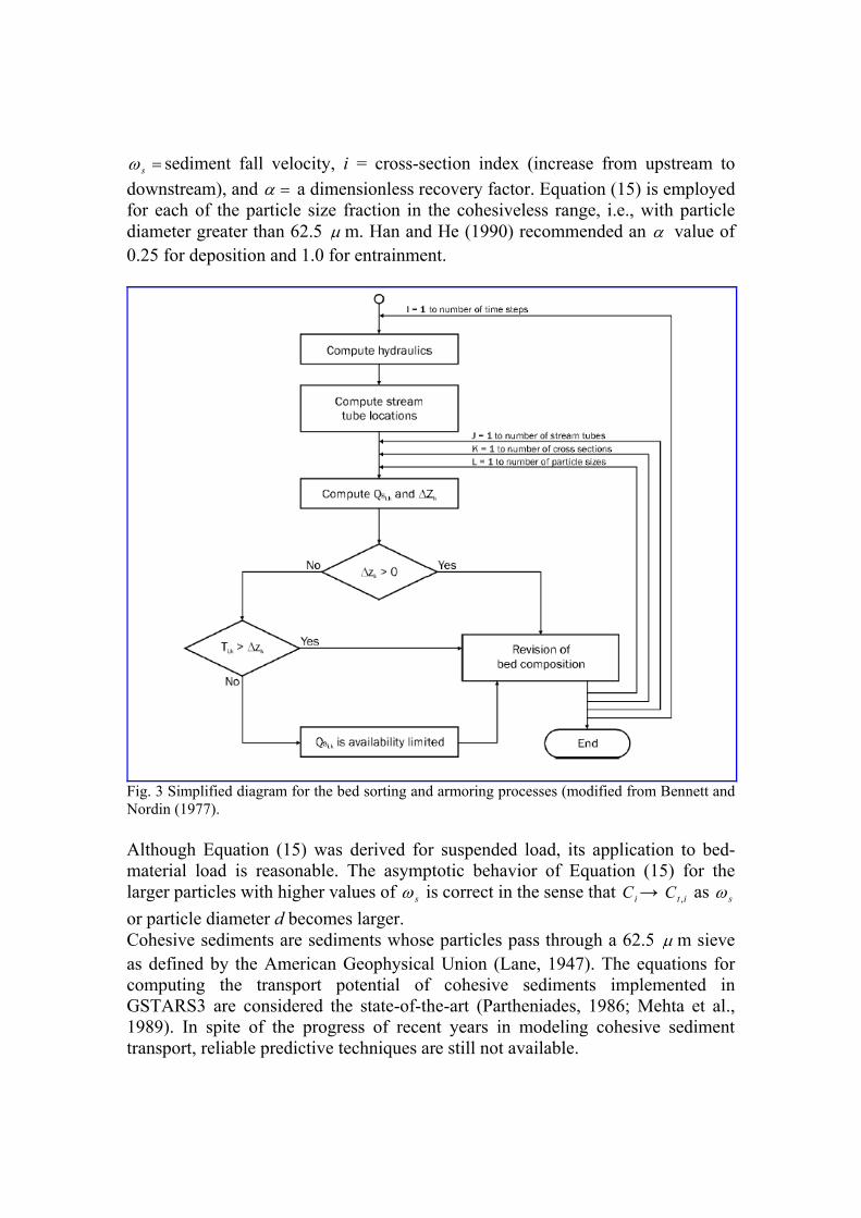
where d = sediment particle diameter, s = specific gravity of sediment in water, g = gravitational acceleration, and ν = viscosity of water. GSTARS models compute sediment transport by size fraction, and particles of different sizes are transported at different rates. Depending on the hydraulic parameters, the incoming sediment distribution, and the bed composition, some particle sizes may be eroded, while others may be deposited or may be immovable. GSTARS computes the carrying capacity for each size fraction presented in the bed with a selected sediment transport formula or method. The actual amount of graded materials moved is computed by the sediment routing Equations (7) and (4). The concept of armor layer is used in the computations. The armor layer prevents the scour or the underlying materials, and the sediment available for transport becomes limited to the amount of sediment entering the reach. However, future hydraulic events, such as an increase of flow velocity, may increase the flow carrying capacity, causing the armor layer to break and restart the erosion processes in the reach. GSTARS uses the bed composition accounting procedure proposed by Bennett and Nordin (1977). The bed accounting is

accomplished by the use of two armor layers for scour and three armor layers for deposition. The thickness of the active layer is defined by the user as proportional to the geometric mean of the largest size class in at least 1 percent of the bed material at that location. Active layer thickness is closely related to the time step duration. Erosion of a particular size of bed material is limited by the amount of sediments of the size class present in the active layer. If the flow-carrying capacity for a particular size class is greater than what is available for transport in the active layer, the term “availability limited” is used (Bennett and Nordin, 1977). If more material is available than that necessary to fulfill the carrying capacity computed by a sediment transport equation, the term “capacity limited” is used. The inactive layer is used when net deposition occurs. The deposition thickness of each size fraction is added to the inactive layer, which in turn is added to the thickness of active layer. The size composition and thickness of the inactive layer is computed first, after which a new active layer is recomputed and the channel bed elevation updated. The overall process is illustrated in Fig. 3. The above procedures are carried out separately along each stream tube. The locations of stream tube boundaries change with changing flow and the sediment conditions and channel geometry at each time step of computation. Bed material composition is stored at each point used to describe the geometry for all the cross-sections. The values of the active and inactive layer thickness are also stored at those points. At the beginning of the next time step, after the new locations of the stream tube boundaries are determined, these values are used to compute the new layer thicknesses and bed composition for each stream tube. Most sediment transport models assume equilibrium sediment transport in the sediment routing process. In this case, if there is a difference between sediment supply from upstream and the sediment transport capacity of the study reach, scour and deposition will occur instantaneously. This assumption is valid for coarse sediment transport where the difference between sediment supply and a river’s transport capacity is not too large. However, there are circumstances in which the spatial-delay and/or time-delay effects are important. For example, reservoir sedimentation processes and the siltation of estuaries are essentially non-equilibrium processes. To model these effects, GSTARS3 uses the method developed by Han (1980). In this method the non-equilibrium sediment transport rate is computed from

( ) ⎥⎦

⎤⎢⎣

⎡⎟⎟⎠

⎞⎜⎜⎝

⎛ Δ−−⎥

⎦

⎤⎢⎣

⎡Δ

−+⎥⎦

⎤⎢⎣

⎡ Δ−−+= −−− q

xx

qCCq

xCCC

C

s

sitit

sitiit

i

αωαω

αωexp1)(exp ,1,)1,1,

(15)

where C = sediment concentration, =tC sediment carrying capacity computed from Equation (4), q = discharge of flow per unit width, =Δx reach length,

=sω sediment fall velocity, i = cross-section index (increase from upstream to downstream), and =α a dimensionless recovery factor. Equation (15) is employed for each of the particle size fraction in the cohesiveless range, i.e., with particle diameter greater than 62.5 μ m. Han and He (1990) recommended an α value of 0.25 for deposition and 1.0 for entrainment.

Fig. 3 Simplified diagram for the bed sorting and armoring processes (modified from Bennett and Nordin (1977). Although Equation (15) was derived for suspended load, its application to bed-material load is reasonable. The asymptotic behavior of Equation (15) for the larger particles with higher values of sω is correct in the sense that iC → itC , as sω or particle diameter d becomes larger. Cohesive sediments are sediments whose particles pass through a 62.5 μ m sieve as defined by the American Geophysical Union (Lane, 1947). The equations for computing the transport potential of cohesive sediments implemented in GSTARS3 are considered the state-of-the-art (Partheniades, 1986; Mehta et al., 1989). In spite of the progress of recent years in modeling cohesive sediment transport, reliable predictive techniques are still not available.

In GSTARS3, the transport of silt and clay is computed separately from the remaining size fractions. GSTARS3 recognizes the presence of clay if any of the particle size fractions given in the input has a geometric mean grain size meand smaller than 0.004 mm. Similarly, the presence of silt is recognized if a size fraction has a meand between 0.004 and 0.0625 mm. There can be any number of particle groups in the clay or silt sizes, up to a maximum of 10 combined groups for cohesive and non-cohesive sediment size groups. For meand ≥ 0.0625 mm, non-cohesive transport formulas or methods will be used. Deposition of clay and silt takes place when the bed shear stress bτ is smaller than the critical bed shear cdτ for deposition.

Minimum Stream Power and Optimum Channel Geometry For alluvial rivers with adjustable boundary, channel width, and channel geometry, there are more unknowns than independent equations available for solving them. Consequently, conventional fluvial hydraulics with sediment transport is indeterminate without using some site specific empirical relationships or assumptions. The minimum energy dissipation rate theory can be derived from thermodynamic analogy between a thermo system and a river system (Yang, 1971). The theory can also be derived directly from mathematical argument (Yang 1992, Yang and Song 1979, 1986). The application of this theory can provide us the needed additional independent theoretical equation(s) for solving fluvial hydraulic problems. The minimum energy dissipation rate theory states that for a closed and dissipative system in a state of dynamic equilibrium condition, its energy dissipation rate must be at its minimum value. The minimum value depends on the constraints applied to the system. If the system is not at its dynamic equilibrium condition, its energy dissipation rate is not at its minimum value. However, the system will adjust itself in such a manner that the energy dissipation rate can be reduced to a minimum and regain equilibrium. Under equilibrium condition, an open system can be converted to a closed system, so the theory is applicable. Due to the dynamic nature of a natural river, it is difficult and may not be possible for a river to reach its true equilibrium condition. However, a river will adjust its width, depth, channel cross-sectional shape and longitudinal bed profile to reduce its energy dissipation rate in the process of self adjustment. GSTARS models utilize the second part of the minimum energy dissipation rate theory, as stated above, for the determination of optimum channel geometry and profile. For open channel flows, the minimum energy dissipation rate theory can be reduced to the minimization of stream power γQS, where γ = specific weight of water, Q = water discharge, and S = longitudinal channel or energy slope. Because γ is a constant for water, the total minimum stream power theory can be expressed by

∫ == QSdxTφ a minimum (16) where x = longitudinal distance along a river. Equation (16) can be discretized as (Chang, 1990)

( ) iiiii

N

iT xSQSQ Δ+= ++

=∑ 11

1 21φ (17)

where N = number of stations along the study reach, =Δ ix distance between stations i and i + 1, and iQ , iS = discharge and slope at station i, respectively. Equation (17) is used in all GSTARS models for the determination of optimum channel geometry. Whether the adjustment should be in the depth or width direction at each time step of computation depends on which one will lead to less stream power. For a channel of multiple stream tubes, only the two exterior tubes can adjust both width and depth. The interior tubes can only adjust its depth. Channel Side Slope Adjustments GSTARS3 and GSTARS2.1 channel geometry adjustment can take place in both lateral and vertical directions. For an interior stream tube, scour or deposition can take place only on the bed, and the computation of depth change is straightforward. For an exterior tube, the change can take place on the bed or at the bank. As erosion progresses, the steepness of the bank slope tends to increase. The maximum allowable bank slope depends on the stability of bank materials. When erosion undermines the lower portion of the bank and the slope increases past a critical value, the bank may collapse to a stable slope. The bank slope should not be allowed to increase beyond a certain critical value. The critical value may vary from case to case, depending on the type of soil and the existence of natural or artificial protection. GSTARS3 and GSTARS2.1 offer the user the option of checking the angle of repose for violation of a known critical value. If this option is chosen, the user must supply the critical angle. The user is also allowed the option of specifying one critical angle above the water surface, and a different critical angle for submerged points. GSTARS3 and GSTARS2.1 scan each cross-section at the end of each time step of computation to determine if any vertical or horizontal adjustments have caused the banks to become too steep. If any violations occur, the two points adjacent to the segment are adjusted vertically until the slope equals the user-provided critical slope. For the situation shown in Fig. 4, the bank is adjusted from abde to edab '' , so the calculated angle, θ, is reduced to the critical angle, cθ . The adjustments are governed by the conservation of mass equation

4321 AAAA +=+ (18)

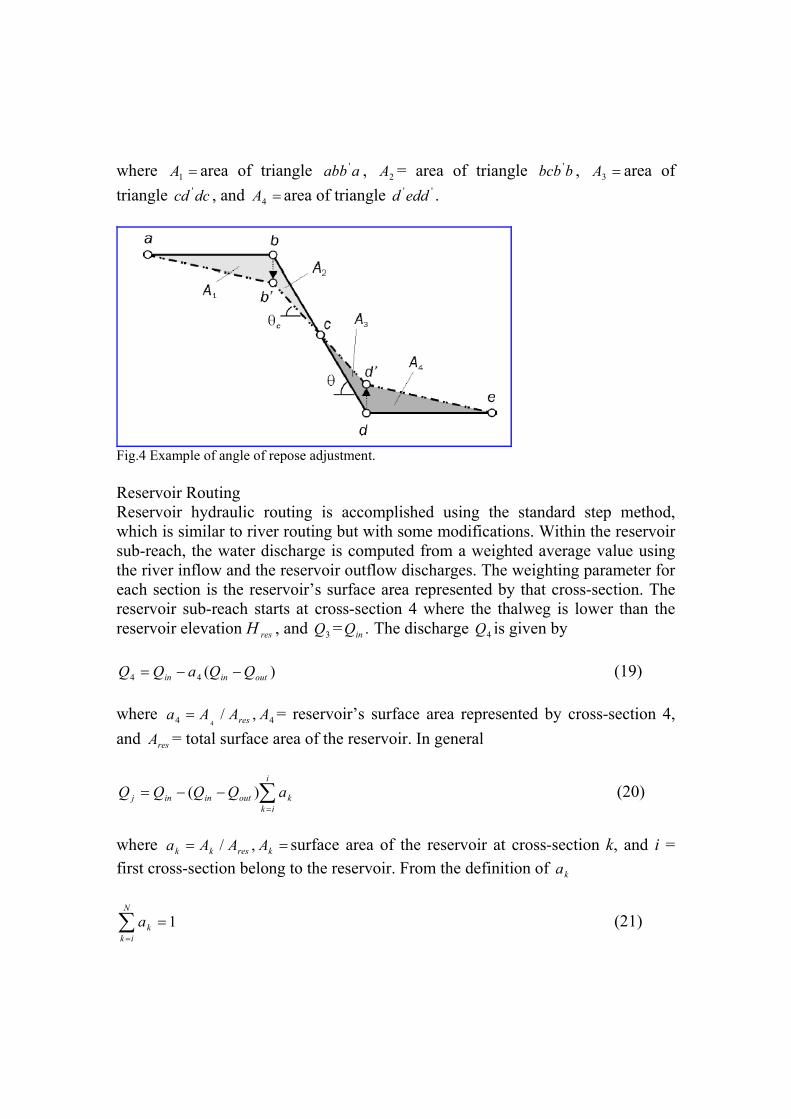
where =1A area of triangle aabb ' , 2A = area of triangle bbcb ' , =3A area of triangle dccd ' , and =4A area of triangle ''eddd .

Fig.4 Example of angle of repose adjustment. Reservoir Routing Reservoir hydraulic routing is accomplished using the standard step method, which is similar to river routing but with some modifications. Within the reservoir sub-reach, the water discharge is computed from a weighted average value using the river inflow and the reservoir outflow discharges. The weighting parameter for each section is the reservoir’s surface area represented by that cross-section. The reservoir sub-reach starts at cross-section 4 where the thalweg is lower than the reservoir elevation H res , and 3Q = inQ . The discharge 4Q is given by

)(44 outinin QQaQQ −−= (19) where 44 ,/

4AAAa res= = reservoir’s surface area represented by cross-section 4,

and resA = total surface area of the reservoir. In general

∑=

−−=i

ikkoutininj aQQQQ )( (20)

where == kreskk AAAa ,/ surface area of the reservoir at cross-section k, and i = first cross-section belong to the reservoir. From the definition of ka

1=∑=

N

ikka (21)

where N = cross-section number at the dam. Water levels at the dam are calculated using level-pool routing assuming that the reservoir water surface is horizontal, i.e.,

tVQQ outin Δ

Δ=− (22)

where VΔ = change in volume of water in the reservoir during time step tΔ . The variation of storage is then used to determine the water level of the reservoir

resH at the dam using a capacity table. The capacity table is a look-up table that is generated incrementally in GSTARS3. Sediment transport formulas can be used for river and reservoir sediment routing. They can be coupled with the non-equilibrium sediment transport formula shown in Equation (15) to obtain more realistic sedimentation distribution in a reservoir. It is generally assumed that bed elevation change ZΔ is uniformly applied to all the cross-section nodes in the wetted perimeter. However, in cases where deposition dominates and rates of bed changes are slow, depositions are formed by filling the lowest part of the channel first, producing flat cross-section profiles. In this case the cross-sectional area change dAΔ can be computed from the change of bed elevation using

ZWAd

Δ=Δ (23) where W = cross-sectional top width in the case of one stream tub, or the stream tube top width in case multiple stream tubes are used. Examples of Application The GSTARS computer models have been applied in the United States and in other countries as a tool for solving river and reservoir sedimentation, environmental, and morphology problems. They have also been used for research and teaching purposes. Some of the application examples will be used herein to illustrate GSTARS models applications. 1 Mississippi River Lock and Dam No.26 Replacement Project At the request of the U.S. Army Corps of Engineers, GSTARS (Molinas and Yang,1986) was applied to simulate and predict local scour at the Mississippi River Lock and Dam No. 26 Replacement Project site near St. Louis, Missouri. Study results were published by Yang et al (1988). Fig. 5 is an aerial view of the Coffer Dam at the construction site. The measured scour pattern is shown in Fig. 6(a). Because GSTARS can not be used for the prediction of local scour due to secondary current, the project site was simplified by cutting off the area of

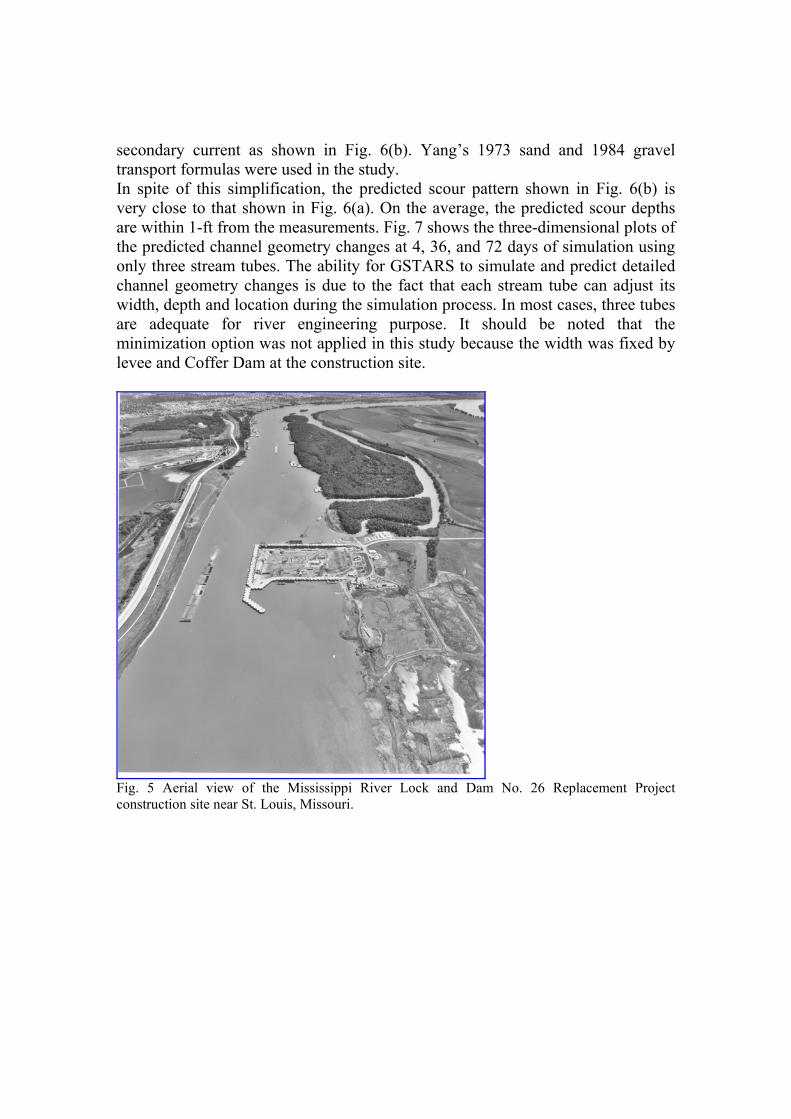
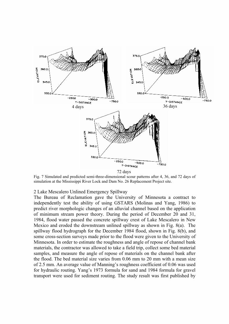
secondary current as shown in Fig. 6(b). Yang’s 1973 sand and 1984 gravel transport formulas were used in the study. In spite of this simplification, the predicted scour pattern shown in Fig. 6(b) is very close to that shown in Fig. 6(a). On the average, the predicted scour depths are within 1-ft from the measurements. Fig. 7 shows the three-dimensional plots of the predicted channel geometry changes at 4, 36, and 72 days of simulation using only three stream tubes. The ability for GSTARS to simulate and predict detailed channel geometry changes is due to the fact that each stream tube can adjust its width, depth and location during the simulation process. In most cases, three tubes are adequate for river engineering purpose. It should be noted that the minimization option was not applied in this study because the width was fixed by levee and Coffer Dam at the construction site.

Fig. 5 Aerial view of the Mississippi River Lock and Dam No. 26 Replacement Project construction site near St. Louis, Missouri.

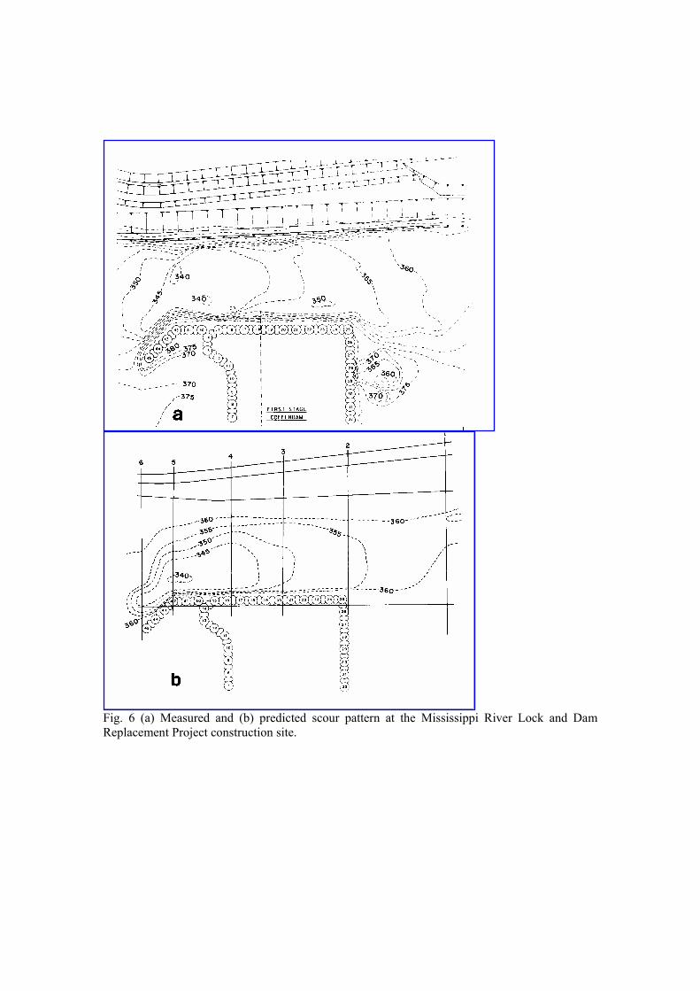
Fig. 6 (a) Measured and (b) predicted scour pattern at the Mississippi River Lock and Dam Replacement Project construction site.

4 days 36 days

72 days

Fig. 7 Simulated and predicted semi-three-dimensional scour patterns after 4, 36, and 72 days of simulation at the Mississippi River Lock and Dam No. 26 Replacement Project site. 2 Lake Mescalero Unlined Emergency Spillway The Bureau of Reclamation gave the University of Minnesota a contract to independently test the ability of using GSTARS (Molinas and Yang, 1986) to predict river morphologic changes of an alluvial channel based on the application of minimum stream power theory. During the period of December 20 and 31, 1984, flood water passed the concrete spillway crest of Lake Mescalero in New Mexico and eroded the downstream unlined spillway as shown in Fig. 8(a). The spillway flood hydrograph for the December 1984 flood, shown in Fig. 8(b), and some cross-section surveys made prior to the flood were given to the University of Minnesota. In order to estimate the roughness and angle of repose of channel bank materials, the contractor was allowed to take a field trip, collect some bed material samples, and measure the angle of repose of materials on the channel bank after the flood. The bed material size varies from 0.06 mm to 20 mm with a mean size of 2.5 mm. An average value of Manning’s roughness coefficient of 0.06 was used for hydraulic routing. Yang’s 1973 formula for sand and 1984 formula for gravel transport were used for sediment routing. The study result was first published by

Song et al (1995). GSTARS 2.0, 2.1, and 3 were later used to re-test the predicted results.

a. b.

Fig.8 (a) Plain view of the channel below the Lake Mescalero emergency spillway, (b) Spillway hydrograph for the December 1984 flood. Fig. 9 shows the initial and measured cross-sections after the flood at Station 0+60 along the emergency spillway. The predicted results using GSTARS3 (Yang and Simões, 2002) with and without the stream power minimization are also shown in Fig. 9. It is apparent that the result obtained using the minimization option more realistically predicts channel width and depth adjustments. Three stream tubes, Yang’s 1973 sand transport and 1984 gravel transport formulas, and Manning’s roughness coefficient of 0.06 used by Song et al. (1995) were also used in the GSTARS3 study.

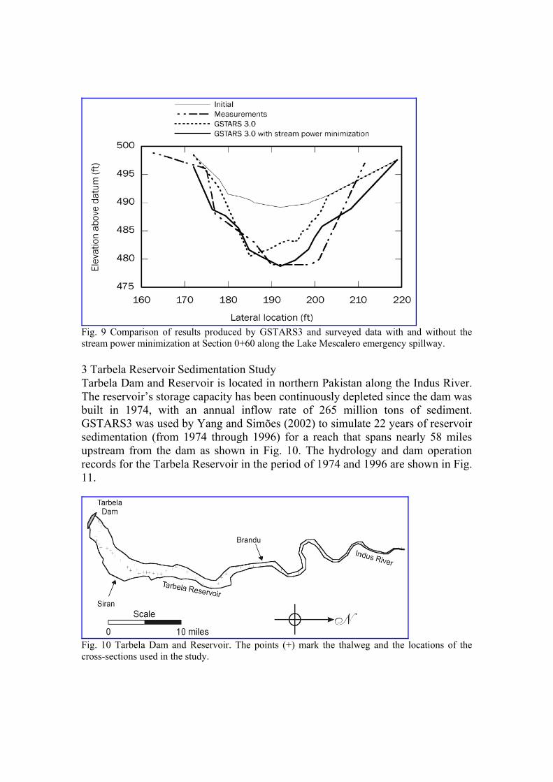
Fig. 9 Comparison of results produced by GSTARS3 and surveyed data with and without the stream power minimization at Section 0+60 along the Lake Mescalero emergency spillway. 3 Tarbela Reservoir Sedimentation Study Tarbela Dam and Reservoir is located in northern Pakistan along the Indus River. The reservoir’s storage capacity has been continuously depleted since the dam was built in 1974, with an annual inflow rate of 265 million tons of sediment. GSTARS3 was used by Yang and Simões (2002) to simulate 22 years of reservoir sedimentation (from 1974 through 1996) for a reach that spans nearly 58 miles upstream from the dam as shown in Fig. 10. The hydrology and dam operation records for the Tarbela Reservoir in the period of 1974 and 1996 are shown in Fig. 11.

Fig. 10 Tarbela Dam and Reservoir. The points (+) mark the thalweg and the locations of the cross-sections used in the study.

Fig. 11 Hydrology and dam operation for Tarbela in the period of 1974 to 1996. Sediments in the Tarbela Reservoir are mainly sand and silt, and Yang’s 1973 formula and Han’s 1980 non-equilibrium transport function were used in the simulation. Only one stream tube was used without using the minimization option because the emphasis of the study was to simulate the longitudinal profile of the delta along the thalweg, especially the location of the front set of the delta and its slope. Fig. 12 shows that the simulated delta longitudinal profile agrees with the 1996 survey result very well, especially the front set of the delta. GSTARS3’s ability to simulate and predict the reservoir delta formation process can be used to determine a reservoir’s loss of capacity, the useful life of a reservoir, and the impact that dam operations have on the reservoir’s deposition pattern.

Fig. 12 Comparison between the measured and simulated longitudinal profiles of the delta in the Tarbela Rivervoir. (Yang and Simões, 2002)

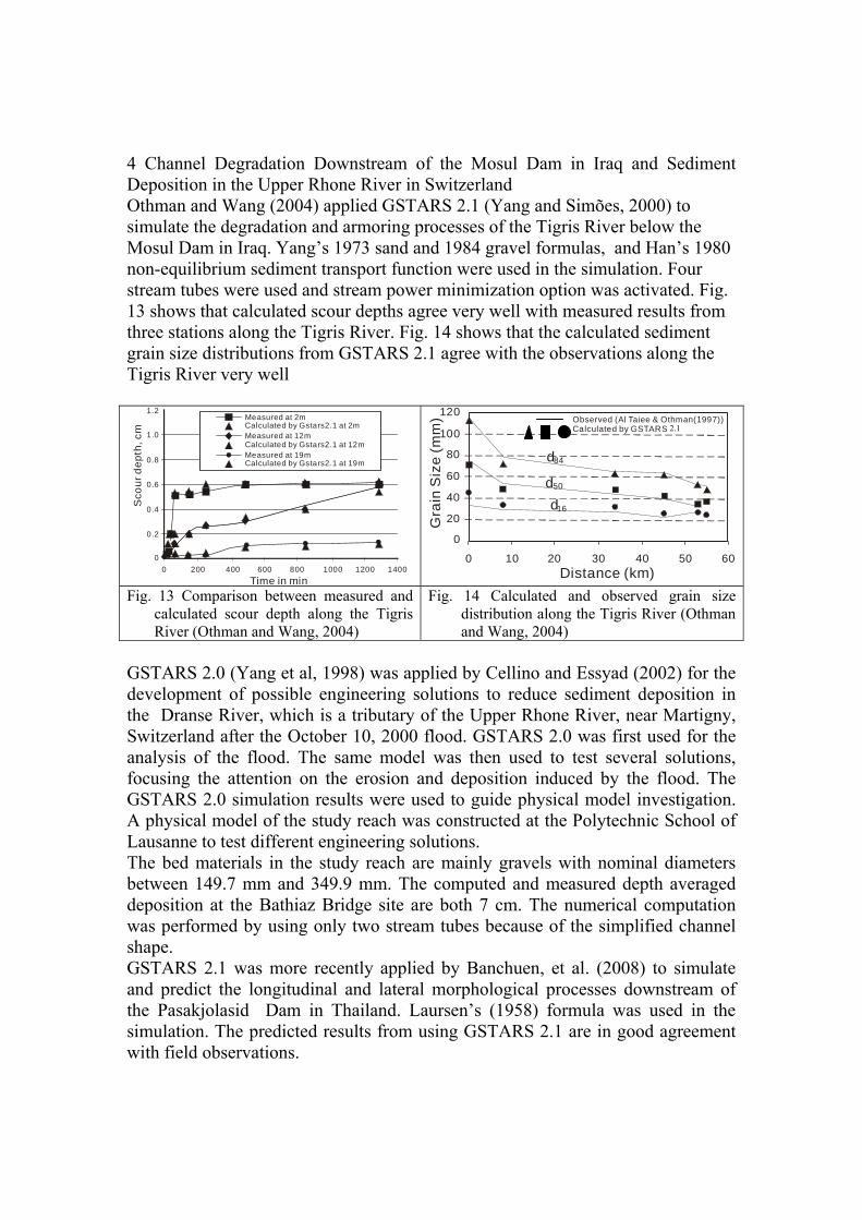
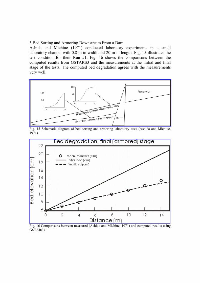
4 Channel Degradation Downstream of the Mosul Dam in Iraq and Sediment Deposition in the Upper Rhone River in Switzerland Othman and Wang (2004) applied GSTARS 2.1 (Yang and Simões, 2000) to simulate the degradation and armoring processes of the Tigris River below the Mosul Dam in Iraq. Yang’s 1973 sand and 1984 gravel formulas, and Han’s 1980 non-equilibrium sediment transport function were used in the simulation. Four stream tubes were used and stream power minimization option was activated. Fig. 13 shows that calculated scour depths agree very well with measured results from three stations along the Tigris River. Fig. 14 shows that the calculated sediment grain size distributions from GSTARS 2.1 agree with the observations along the Tigris River very well

00 200 400 600 800 1000 1200 1400

0.2

0.4

0.6

0.8

1.0

1.2Measured at 2mCalculated by Gstars2.1 at 2m

Calculated by Gstars2.1 at 12m

Calculated by Gstars2.1 at 19m

Measured at 12m

Measured at 19m

Time in min

Sco

ur d

epth

, cm

d

dd

84

50

16

0

20

40

60

80

100

120

0 10 20 30 40 50 60Distance (km)

Gra

in S

ize

(mm

) Observed (Al Taiee & Othman(1997))Calculated by GSTARS

Fig. 13 Comparison between measured and calculated scour depth along the Tigris River (Othman and Wang, 2004)

Fig. 14 Calculated and observed grain size distribution along the Tigris River (Othman and Wang, 2004)

GSTARS 2.0 (Yang et al, 1998) was applied by Cellino and Essyad (2002) for the development of possible engineering solutions to reduce sediment deposition in the Dranse River, which is a tributary of the Upper Rhone River, near Martigny, Switzerland after the October 10, 2000 flood. GSTARS 2.0 was first used for the analysis of the flood. The same model was then used to test several solutions, focusing the attention on the erosion and deposition induced by the flood. The GSTARS 2.0 simulation results were used to guide physical model investigation. A physical model of the study reach was constructed at the Polytechnic School of Lausanne to test different engineering solutions. The bed materials in the study reach are mainly gravels with nominal diameters between 149.7 mm and 349.9 mm. The computed and measured depth averaged deposition at the Bathiaz Bridge site are both 7 cm. The numerical computation was performed by using only two stream tubes because of the simplified channel shape. GSTARS 2.1 was more recently applied by Banchuen, et al. (2008) to simulate and predict the longitudinal and lateral morphological processes downstream of the Pasakjolasid Dam in Thailand. Laursen’s (1958) formula was used in the simulation. The predicted results from using GSTARS 2.1 are in good agreement with field observations.

2.1

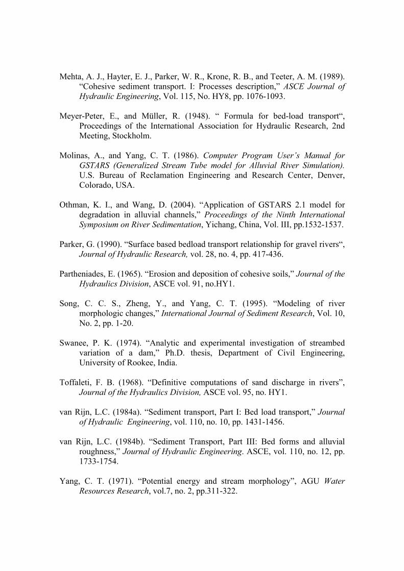
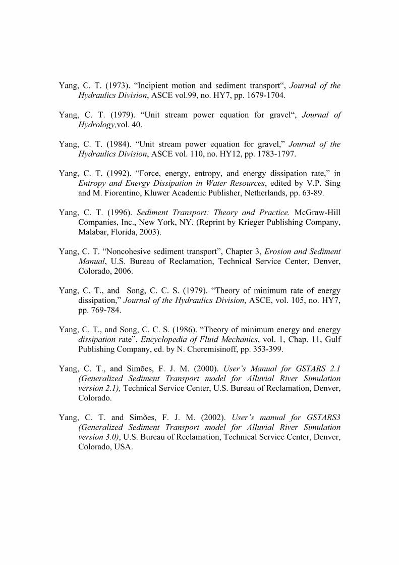
5 Bed Sorting and Armoring Downstream From a Dam Ashida and Michiue (1971) conducted laboratory experiments in a small laboratory channel with 0.8 m in width and 20 m in length. Fig. 15 illustrates the test condition for their Run #1. Fig. 16 shows the comparisons between the computed results from GSTARS3 and the measurements at the initial and final stage of the tests. The computed bed degradation agrees with the measurements very well.

River bed a fter dam rem ova l Dam

Reservior

River bed before dam rem ova l

100

100

1

1

10

10

50

50

0

0

0.1

0.1

Fig. 15 Schematic diagram of bed sorting and armoring laboratory tests (Ashida and Michiue, 1971).

Fig. 16 Comparisons between measured (Ashida and Michiue, 1971) and computed results using GSTARS3.

6 Reservoir Delta Formation Swamee (1974) conducted laboratory tests for the development of reservoir delta. Fig. 17(a) shows comparisons between measured and computer profiles from GSTARS3 with three different values of roughness coefficient. Fig. 17(b) shows that predicted delta development agrees with laboratory test results very well. The minor local differences between the computed and measured results shown in Fig. 17(b) are due to the presence of bed forms.

n= 0.010n= 0.015n= 0.020

95

90

85

80

75

70

6525 20 15 10 5 0

Swanee (1974)

Elev

atio

n (m

)

Distanc e upstream (a)

GSTARS 3.0Initia l bed12 hours24 hours

Swanee (1974)

24 hours12 hours

95

90

85

80

75

70

6525 20 15 10 5 0

Bed

elev

atio

n (c

m)

Distanc e upstream (m) (b)

Fig. 17 Comparisons between laboratory tests by Swamee (1974) and predicted results from GSTARS3. (a) Water surface profile, (b) Delta development.

Summary and Conclusions

This paper provides a brief summary of the theories and concepts used in the GSTARS computer models. Examples based on field and laboratory data are used to illustrate the application of GSTARS models to a wide range of river and reservoir sedimentation projects. The simulated and predicted results are in good agreement with field and laboratory measurements. The executable codes and user’s manuals of GSTARS 2.1 and GSTARS3 can be downloaded from website (http://www.engr.colostate.edu/ce), then click Academic Faculty/Hydraulic Engineering/Chih Ted Yang/Personal Website/GSTARS, free of charge.

References

Ackers, P., and White, W. R. (1973). “ Sediment transport: new approach and analysis“, Journal of the Hydraulics Division, ASCE, vol. 99, no. HY11.

Alonso, C. V. (1980). “Selecting a Formula to Estimate Sediment Transport

Capacity in Nonvegetated Channels,” CREAMS (A Field Scale Model for Chemicals, Runoff, and Erosion for Agricultural Management System), W.G. Knisel editor, U.S. Department of Agriculture Conservation Research Report no. 26, Chapter 5, pp. 426-439.

ASCE (1982), ASCE Task Committee on Relations between Morphology of Small

Streams and Sediment Yield of the Committee on Sedimentation of the Hydraulics Division, “Relationships between morphology of small streams and sediment yields“ , Journal of the Hydraulics Division, ASCE, vol. 108, no. HY11, pp. 1328-1365.

Ashida, K., and Michiue, M. (1971). “An investigation of river bed degradation

downstream of a dam,” Proceedings of the IAHR XIV Congress, Vol. 3. Ashida, K., and Michiue, M. (1972). “Study on hydraulic resistance and bed load

transport rate in alluvial streams”, Proceedings of JSCE, pp.59-69 (in Japanese).

Banchuen, S., Tingsanchali, T., and Chinnarasri, C. (2008). “Comparison between

GSTARS 2.1 and HTC-6 river morphological models,” International Journal of Hydrological Sciences, IAHS August.

Bennett, J., and Nordin, C. (1977). “Simulation of sediment transport and

armouring,” Hydrological Sciences Bulletin, vol. 22, pp. 555-569.

Cellino, M., and Essyad, K. (2002). “Reduction of sediment deposition by introducing an artificial stony bank. A practical example in Upper Rhone River, Switzerland” Proceedings of the International Conference on Fluvial Hydraulics, Louvain-La-Neuve, Belgium,River, Flow 2002 edited by D. Bousmar and Y. Zech, A. A. Balkema Bublishers, Lisse/Abingdon/Exton (PA)/Tokyo, pp.951-959.

Chang, H. (1990). “Generalized computer program FLUVIAL-12“, Mathematical

Model for Erodible Channels User’s Manual. DuBoys, M. P. (1879). “Le Rhône et les rivières à lit afflouillable“, Annals de

Ponts et Chaussée, vol. 18, no. 5, pp. 141-195 (in French). Engelund, F. , and Hansen, E. (1972). A monograph on sediment transport in

alluvial streams, Teknish Forlag, Technical Press, Copenhagen, Demark. Han, Q. (1980). “A study on the nonequilibrium transportation of suspended

load.” Proceedings of the International Symposium on River Sedimentation, Beijing, China, pp. 793-802. (In Chinese.)

Han, Q., and He, M. (1990). “A mathematical model for reservoir sedimentation

and fluvial processes,” International Journal of Sediment Research, vol. 5, no. 2, IRTCES, pp. 43-84.

IRTCES (1985). Lecture notes of the training course on reservoir sedimentation.

International Research and Training Center on Erosion and Sedimentation, Sediment Reseach Laboratory of Tsinghua University, Beijing, China.

Krone, R. B. (1962). Flume studies of the transport of sediment in estuarial

process, Hydraulic Engineering Laboratory and Sanitary Enginering Research Laboratory, University of California, Berkeley, CA.

Lane, E. W. (1947). “Report of the Subcommittee on Sediment Terminology,”

Transaction of the American Geophysical Union, vol. 28, no. 6, Washington, D.C.

Layrsen, E. M. (1958). “The total sediment load of streams“, Journal of the

Hydraulics Division, ASCE vol. 84, no. HY1. Madden, E. (1993). Modified Laursen method for estimating bed-material

sediment load, USACE-WES, Contract Report HL-93-3.

Mehta, A. J., Hayter, E. J., Parker, W. R., Krone, R. B., and Teeter, A. M. (1989). “Cohesive sediment transport. I: Processes description,” ASCE Journal of Hydraulic Engineering, Vol. 115, No. HY8, pp. 1076-1093.

Meyer-Peter, E., and Müller, R. (1948). “ Formula for bed-load transport“,

Proceedings of the International Association for Hydraulic Research, 2nd Meeting, Stockholm.

Molinas, A., and Yang, C. T. (1986). Computer Program User’s Manual for

GSTARS (Generalized Stream Tube model for Alluvial River Simulation). U.S. Bureau of Reclamation Engineering and Research Center, Denver, Colorado, USA.

Othman, K. I., and Wang, D. (2004). “Application of GSTARS 2.1 model for

degradation in alluvial channels,” Proceedings of the Ninth International Symposium on River Sedimentation, Yichang, China, Vol. III, pp.1532-1537.

Parker, G. (1990). “Surface based bedload transport relationship for gravel rivers“,

Journal of Hydraulic Research, vol. 28, no. 4, pp. 417-436. Partheniades, E. (1965). “Erosion and deposition of cohesive soils,” Journal of the

Hydraulics Division, ASCE vol. 91, no.HY1. Song, C. C. S., Zheng, Y., and Yang, C. T. (1995). “Modeling of river

morphologic changes,” International Journal of Sediment Research, Vol. 10, No. 2, pp. 1-20.

Swanee, P. K. (1974). “Analytic and experimental investigation of streambed

variation of a dam,” Ph.D. thesis, Department of Civil Engineering, University of Rookee, India.

Toffaleti, F. B. (1968). “Definitive computations of sand discharge in rivers”,

Journal of the Hydraulics Division, ASCE vol. 95, no. HY1. van Rijn, L.C. (1984a). “Sediment transport, Part I: Bed load transport,” Journal

of Hydraulic Engineering, vol. 110, no. 10, pp. 1431-1456. van Rijn, L.C. (1984b). “Sediment Transport, Part III: Bed forms and alluvial

roughness,” Journal of Hydraulic Engineering. ASCE, vol. 110, no. 12, pp. 1733-1754.

Yang, C. T. (1971). “Potential energy and stream morphology”, AGU Water

Resources Research, vol.7, no. 2, pp.311-322.

Yang, C. T. (1973). “Incipient motion and sediment transport“, Journal of the

Hydraulics Division, ASCE vol.99, no. HY7, pp. 1679-1704. Yang, C. T. (1979). “Unit stream power equation for gravel“, Journal of

Hydrology,vol. 40. Yang, C. T. (1984). “Unit stream power equation for gravel,” Journal of the

Hydraulics Division, ASCE vol. 110, no. HY12, pp. 1783-1797. Yang, C. T. (1992). “Force, energy, entropy, and energy dissipation rate,” in

Entropy and Energy Dissipation in Water Resources, edited by V.P. Sing and M. Fiorentino, Kluwer Academic Publisher, Netherlands, pp. 63-89.

Yang, C. T. (1996). Sediment Transport: Theory and Practice. McGraw-Hill

Companies, Inc., New York, NY. (Reprint by Krieger Publishing Company, Malabar, Florida, 2003).

Yang, C. T. “Noncohesive sediment transport”, Chapter 3, Erosion and Sediment

Manual, U.S. Bureau of Reclamation, Technical Service Center, Denver, Colorado, 2006.

Yang, C. T., and Song, C. C. S. (1979). “Theory of minimum rate of energy

dissipation,” Journal of the Hydraulics Division, ASCE, vol. 105, no. HY7, pp. 769-784.

Yang, C. T., and Song, C. C. S. (1986). “Theory of minimum energy and energy

dissipation rate”, Encyclopedia of Fluid Mechanics, vol. 1, Chap. 11, Gulf Publishing Company, ed. by N. Cheremisinoff, pp. 353-399.

Yang, C. T., and Simões, F. J. M. (2000). User’s Manual for GSTARS 2.1

(Generalized Sediment Transport model for Alluvial River Simulation version 2.1), Technical Service Center, U.S. Bureau of Reclamation, Denver, Colorado.

Yang, C. T. and Simões, F. J. M. (2002). User’s manual for GSTARS3

(Generalized Sediment Transport model for Alluvial River Simulation version 3.0), U.S. Bureau of Reclamation, Technical Service Center, Denver, Colorado, USA.

Yang, C. T., Molinas, A., and Song, C. C. S. (1988). “GSTARS – Generalized Stream Tube model for Alluvial River Simulation,” Twelve Selected Computer Stream Sedimentation Models Developed in the United States, Subcommittee on Sedimentation , Interagency Advisory Committee on Water Data, Interagency Ad Hoc Sedimentation Work Group, edited by S-S. Fan, Federal Energy Regulatory Commission. Washington, D.C., USA.

Yang, C. T., Molinas, A., and Wu, B. (1996). “Sediment transport in the Yellow

River”, Journal of Hydraulic Engineering, ASCE vol.122 no. 5. Yang, C. T., Treviño, M. A., and Simões, F. J. M. (1998). User’s Manual for

GSTARS 2.0 (Generalized Stream Tube model for Alluvial River simulation version 2.0), U.S. Bureau of Reclamation, Technical Service Center, Denver, Colorado, USA.