1 Mplus Short Courses Topic 3 Growth Modeling With Latent Variables Using Mplus: Introductory And Intermediate Growth Models Linda K. Muthén Bengt Muthén Copyright © 2010 Muthén & Muthén www.statmodel.com 05/17/2010 2 General Latent Variable Modeling Framework 7 Typical Examples Of Growth Modeling 15 Basic Modeling Ideas 24 Growth Modeling Frameworks 28 The Latent Variable Growth Model In Practice 41 Growth Model Estimation, Testing, And Model Modification 55 Simple Examples Of Growth Modeling 64 Covariates In The Growth Model 84 Centering 99 Non-Linear Growth 106 Growth Model With Free Time Scores 108 Piecewise Growth Modeling 120 Intermediate Growth Models 127 Growth Model With Individually Varying Times Of Observation And Random Slopes For Time-Varying Covariates 128 Alternative Models With Time-Varying Covariates 138 Regressions Among Random Effects 162 Growth Modeling With Parallel Processes 172 Categorical Outcomes: Logistic and Probit Regression 185 Growth Modeling With Categorical Outcomes 192 References 213 Table Of Contents

Welcome message from author
This document is posted to help you gain knowledge. Please leave a comment to let me know what you think about it! Share it to your friends and learn new things together.
Transcript
1
Mplus Short CoursesTopic 3
Growth Modeling With Latent Variables Using Mplus:
Introductory And Intermediate Growth ModelsLinda K. Muthén
Bengt Muthén
Copyright © 2010 Muthén & Muthénwww.statmodel.com
05/17/2010
2
General Latent Variable Modeling Framework 7Typical Examples Of Growth Modeling 15
Basic Modeling Ideas 24Growth Modeling Frameworks 28The Latent Variable Growth Model In Practice 41
Growth Model Estimation, Testing, And Model Modification 55Simple Examples Of Growth Modeling 64
Covariates In The Growth Model 84Centering 99Non-Linear Growth 106Growth Model With Free Time Scores 108Piecewise Growth Modeling 120
Intermediate Growth Models 127Growth Model With Individually Varying Times Of Observation
And Random Slopes For Time-Varying Covariates 128Alternative Models With Time-Varying Covariates 138Regressions Among Random Effects 162Growth Modeling With Parallel Processes 172Categorical Outcomes: Logistic and Probit Regression 185
Growth Modeling With Categorical Outcomes 192References 213
Table Of Contents

3
• Inefficient dissemination of statistical methods:– Many good methods contributions from biostatistics,
psychometrics, etc are underutilized in practice• Fragmented presentation of methods:
– Technical descriptions in many different journals– Many different pieces of limited software
• Mplus: Integration of methods in one framework– Easy to use: Simple, non-technical language, graphics– Powerful: General modeling capabilities
Mplus Background
• Mplus versions
• Mplus team: Linda & Bengt Muthén, Thuy Nguyen, Tihomir Asparouhov, Michelle Conn, Jean Maninger
4
Mplus Background
‒ V1: November 1998‒ V3: March 2004‒ V5: November 2007‒ V6: April, 2010
‒ V2: February 2001‒ V4: February 2006‒ V5.21: May 2009
5
Statistical Analysis With Latent VariablesA General Modeling Framework
Statistical Concepts Captured By Latent Variables
• Measurement errors• Factors• Random effects• Frailties, liabilities• Variance components• Missing data
• Latent classes• Clusters• Finite mixtures• Missing data
Continuous Latent Variables Categorical Latent Variables
6
Statistical Analysis With Latent VariablesA General Modeling Framework (Continued)
• Factor analysis models• Structural equation models• Growth curve models• Multilevel models
• Latent class models• Mixture models• Discrete-time survival models• Missing data models
Models That Use Latent Variables
Mplus integrates the statistical concepts captured by latent variables into a general modeling framework that includes not only all of the models listed above but also combinations and extensions of these models.
Continuous Latent Variables Categorical Latent Variables
7
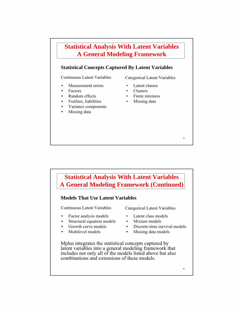
• Observed variablesx background variables (no model structure)y continuous and censored outcome variablesu categorical (dichotomous, ordinal, nominal) and
count outcome variables• Latent variables
f continuous variables– interactions among f’s
c categorical variables– multiple c’s
General Latent Variable Modeling Framework
8
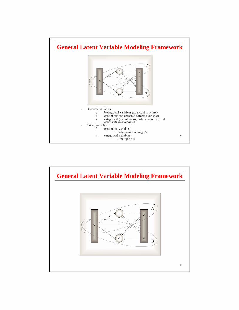
General Latent Variable Modeling Framework
9
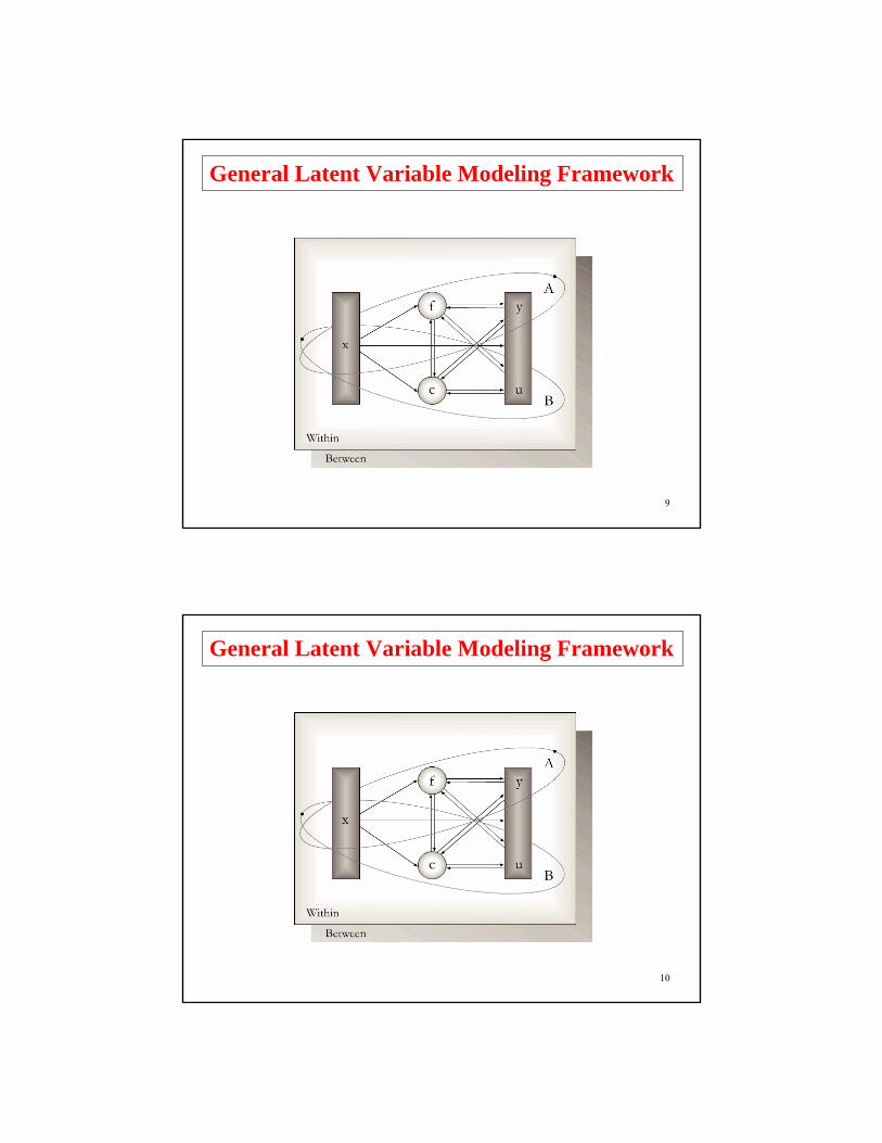
General Latent Variable Modeling Framework
10
General Latent Variable Modeling Framework
11
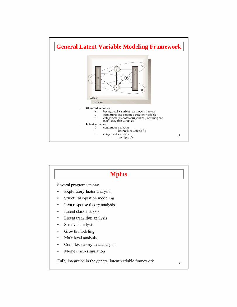
General Latent Variable Modeling Framework
• Observed variablesx background variables (no model structure)y continuous and censored outcome variablesu categorical (dichotomous, ordinal, nominal) and
count outcome variables• Latent variables
f continuous variables– interactions among f’s
c categorical variables– multiple c’s
12
MplusSeveral programs in one • Exploratory factor analysis• Structural equation modeling• Item response theory analysis• Latent class analysis• Latent transition analysis• Survival analysis• Growth modeling• Multilevel analysis• Complex survey data analysis• Monte Carlo simulation
Fully integrated in the general latent variable framework

13
Overview Of Mplus Courses
• Topic 1. August 20, 2009, Johns Hopkins University: Introductory - advanced factor analysis and structural equation modeling with continuous outcomes
• Topic 2. August 21, 2009, Johns Hopkins University: Introductory - advanced regression analysis, IRT, factor analysis and structural equation modeling with categorical, censored, and count outcomes
• Topic 3. March 22, 2010, Johns Hopkins University: Introductory and intermediate growth modeling
• Topic 4. March 23, 2010, Johns Hopkins University:Advanced growth modeling, survival analysis, and missing data analysis
14
Overview Of Mplus Courses (Continued)
• Topic 5. August 16, 2010, Johns Hopkins University: Categorical latent variable modeling with cross-sectional data• Topic 6. August 17, 2010, Johns Hopkins University: Categorical latent variable modeling with longitudinal data• Extra Topic. August 18, 2010, Johns Hopkins University: What’s new in Mplus version 6?
• Topic 7. March, 2011, Johns Hopkins University:Multilevel modeling of cross-sectional data
• Topic 8. March, 2011, Johns Hopkins University: Multilevel modeling of longitudinal data
15
Typical Examples Of Growth Modeling
16
LSAY Data
Longitudinal Study of American Youth (LSAY)
• Two cohorts measured each year beginning in 1987– Cohort 1 - Grades 10, 11, and 12– Cohort 2 - Grades 7, 8, 9, 10, 11, and 12
• Each cohort contains approximately 60 schools with approximately 60 students per school
• Variables - math and science achievement items, math and science attitude measures, and background variables from parents, teachers, and school principals
• Approximately 60 items per test with partial item overlap acrossgrades - adaptive tests
17
Grade
Ave
rage
Sco
re
Male YoungerFemale YoungerMale OlderFemale Older
7 8 9 10 11 1250
52
54
56
58
60
62
64
66
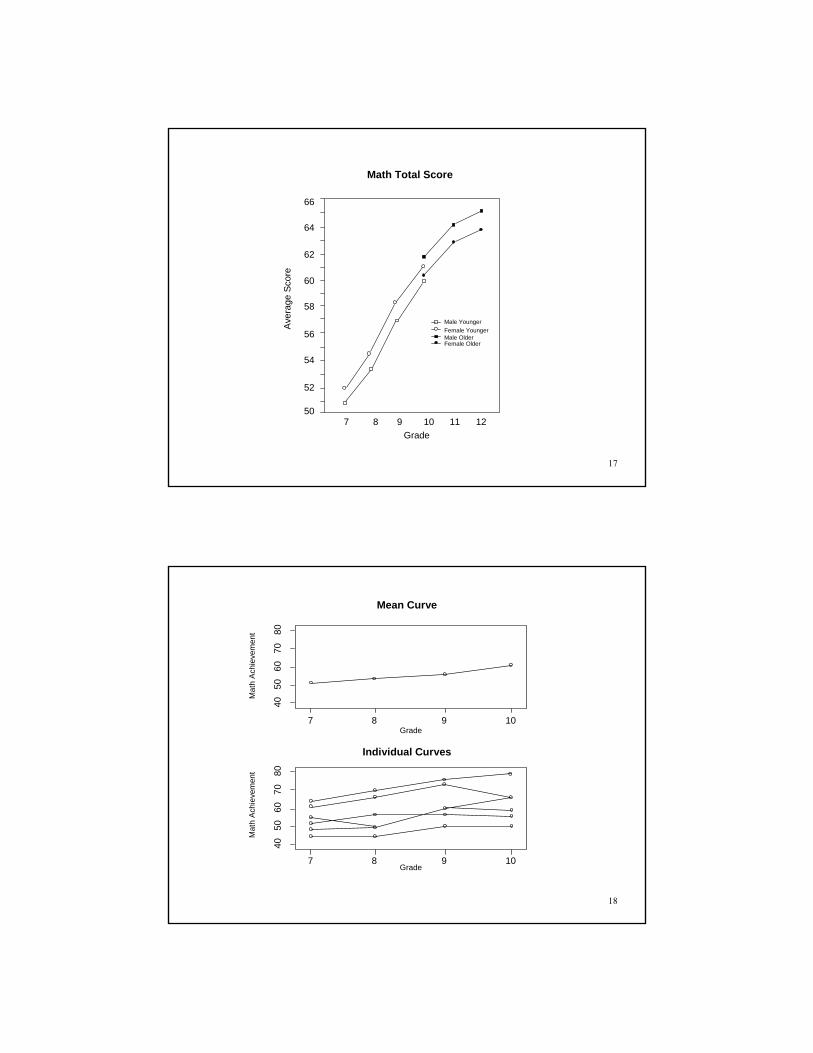
Math Total Score
18
Grade
Mat
h A
chie
vem
ent
7 8 9 10
4050
6070
80
7 8 9 10
Mat
h A
chie
vem
ent
Grade
4050
6070
80
Mean Curve
Individual Curves

19
Grade
Mat
h A
chie
vem
ent
7 8 9 10
7 8 9 10
Mat
h A
ttitu
de
Grade
Sample Means for Attitude Towards Math
4050
6070
8010
1112
1314
15
Sample Means for Math
20
Maternal Health Project Data
Maternal Health Project (MHP)• Mothers who drank at least three drinks a week during
their first trimester plus a random sample of mothers who used alcohol less often
• Mothers measured at fourth month and seventh month of pregnancy, at delivery, and at 8, 18, and 36 months postpartum
• Offspring measured at 0, 8, 18 and 36 months• Variables for mothers - demographic, lifestyle, current
environment, medical history, maternal psychological status, alcohol use, tobacco use, marijuana use, other illicit drug use
• Variables for offspring - head circumference, height, weight, gestational age, gender, and ethnicity
21
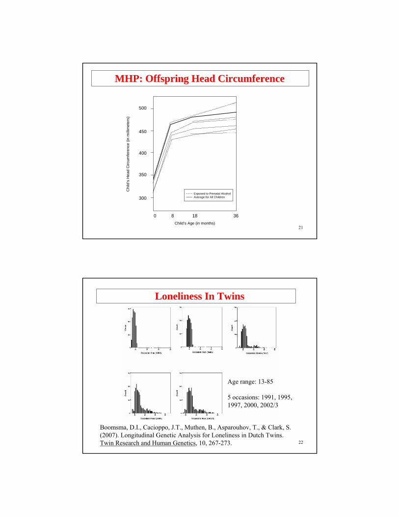
MHP: Offspring Head Circumference
0 8 18 36
300
350
400
450
500
Chi
ld’s
Hea
d C
ircum
fere
nce
(in m
illim
eter
s)
Child’s Age (in months)
Exposed to Prenatal AlcoholAverage for All Children
22
Loneliness In Twins
Boomsma, D.I., Cacioppo, J.T., Muthen, B., Asparouhov, T., & Clark, S. (2007). Longitudinal Genetic Analysis for Loneliness in Dutch Twins. Twin Research and Human Genetics, 10, 267-273.
Age range: 13-85
5 occasions: 1991, 1995, 1997, 2000, 2002/3

23
Loneliness In Twins
Males Females
I feel lonely
Nobody loves me
24
Basic Modeling Ideas
25
Longitudinal Data: Three Approaches
Three modeling approaches for the regression of outcome on time (n is sample size, T is number of timepoints):
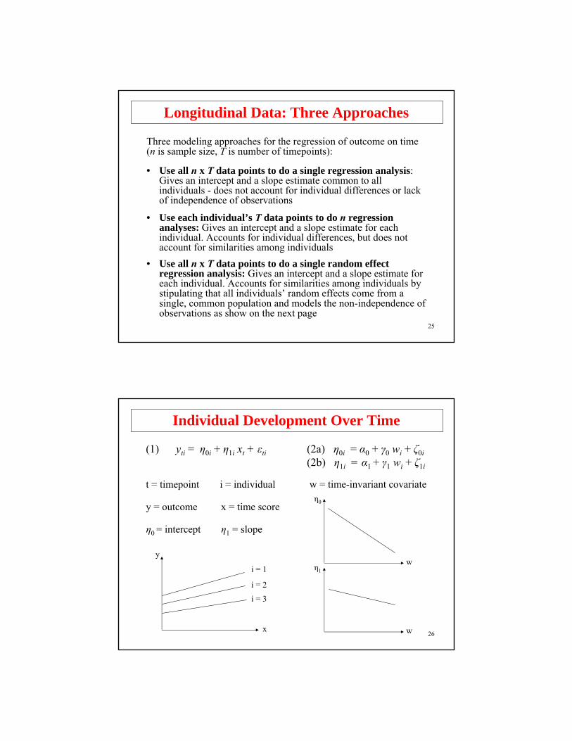
• Use all n x T data points to do a single regression analysis: Gives an intercept and a slope estimate common to all individuals - does not account for individual differences or lack of independence of observations
• Use each individual’s T data points to do n regression analyses: Gives an intercept and a slope estimate for each individual. Accounts for individual differences, but does not account for similarities among individuals
• Use all n x T data points to do a single random effect regression analysis: Gives an intercept and a slope estimate for each individual. Accounts for similarities among individuals by stipulating that all individuals’ random effects come from a single, common population and models the non-independence of observations as show on the next page
26
Individual Development Over Time
(1) yti = η0i + η1i xt + εti
t = timepoint i = individual
y = outcome x = time score
η0 = intercept η1 = slope
(2a) η0i = α0 + γ0 wi + ζ0i(2b) η1i = α1 + γ1 wi + ζ1i
w = time-invariant covariate
i = 1
i = 2
i = 3
y
x
η1
w
η0
w

27
(1) yti = η0i + η1i xt + εti
(2a) η0i = α0 + γ0 wi + ζ0i
(2b) η1i = α1 + γ1 wi + ζ1i
Individual Development Over Time
y1
w
y2 y3 y4
η0 η1
ε1 ε2 ε3 ε4
t = 1 t = 2 t = 3 t = 4
i = 1
i = 2
i = 3
y
x
28
Growth Modeling Frameworks
29
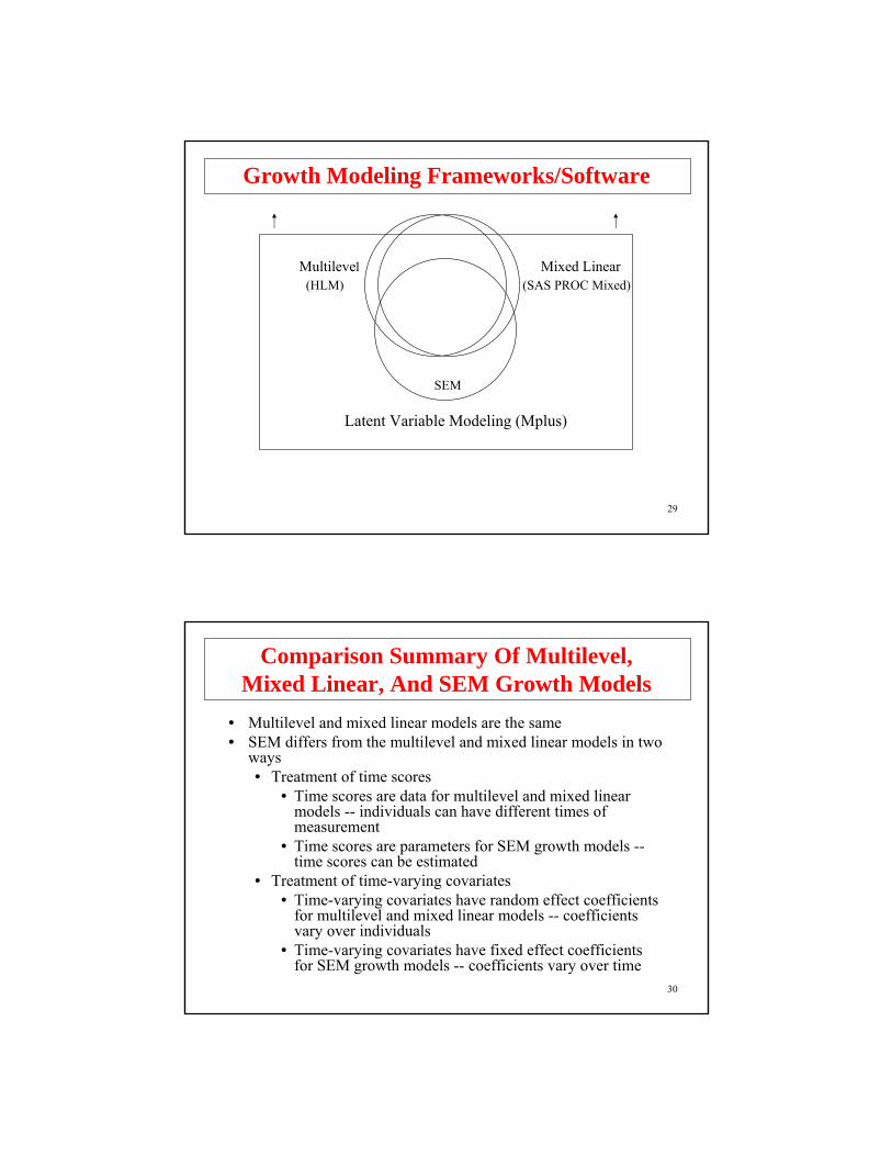
Growth Modeling Frameworks/Software
Multilevel Mixed Linear
SEM
Latent Variable Modeling (Mplus)
(SAS PROC Mixed)(HLM)
30
Comparison Summary Of Multilevel, Mixed Linear, And SEM Growth Models
• Multilevel and mixed linear models are the same• SEM differs from the multilevel and mixed linear models in two
ways• Treatment of time scores
• Time scores are data for multilevel and mixed linear models -- individuals can have different times of measurement
• Time scores are parameters for SEM growth models --time scores can be estimated
• Treatment of time-varying covariates• Time-varying covariates have random effect coefficients
for multilevel and mixed linear models -- coefficients vary over individuals
• Time-varying covariates have fixed effect coefficients for SEM growth models -- coefficients vary over time

31
Random Effects: MultilevelAnd Mixed Linear Modeling
Individual i (i = 1, 2, …, n) observed at time point t (t = 1, 2, … T).
Multilevel model with two levels (e.g. Raudenbush & Bryk,2002, HLM).
• Level 1: yti = η0i + η1i xti + κi wti + εti (39)
• Level 2: η0i = α0 + γ0 wi + ζ0i (40)η1i = α1 + γ1 wi + ζ1i (41)κi = α + γ wi + ζi (42)
32
Random Effects: MultilevelAnd Mixed Linear Modeling (Continued)
Mixed linear model:
yti = fixed part + random part (43)= α0 + γ0 wi + (α1 + γ1 wi) xti + (α + γ wi) wti (44)
+ ζ0i + ζ1i xti + ζi wti + εti . (45)
E.g. “time X wi” refers to γ1 (e.g. Rao, 1958; Laird &Ware, 1982; Jennrich & Sluchter, 1986; Lindstrom & Bates,1988; BMDP5V; Goldstein, 2003, MLwiN; SAS PROCMIXED-Littell et al. 1996 and Singer, 1999).
33
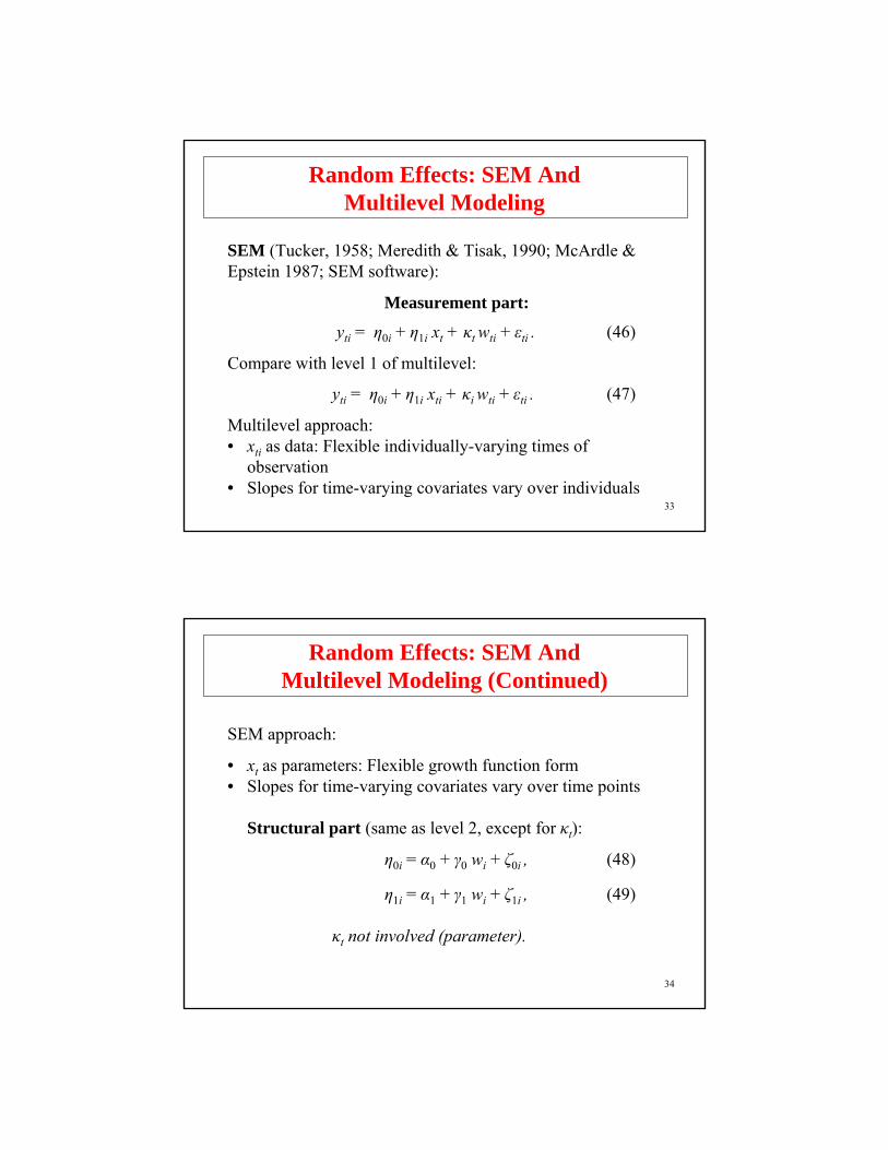
Random Effects: SEM AndMultilevel Modeling
SEM (Tucker, 1958; Meredith & Tisak, 1990; McArdle &Epstein 1987; SEM software):
Measurement part:
yti = η0i + η1i xt + κt wti + εti . (46)
Compare with level 1 of multilevel:
yti = η0i + η1i xti + κi wti + εti . (47)
Multilevel approach:• xti as data: Flexible individually-varying times of
observation• Slopes for time-varying covariates vary over individuals
34
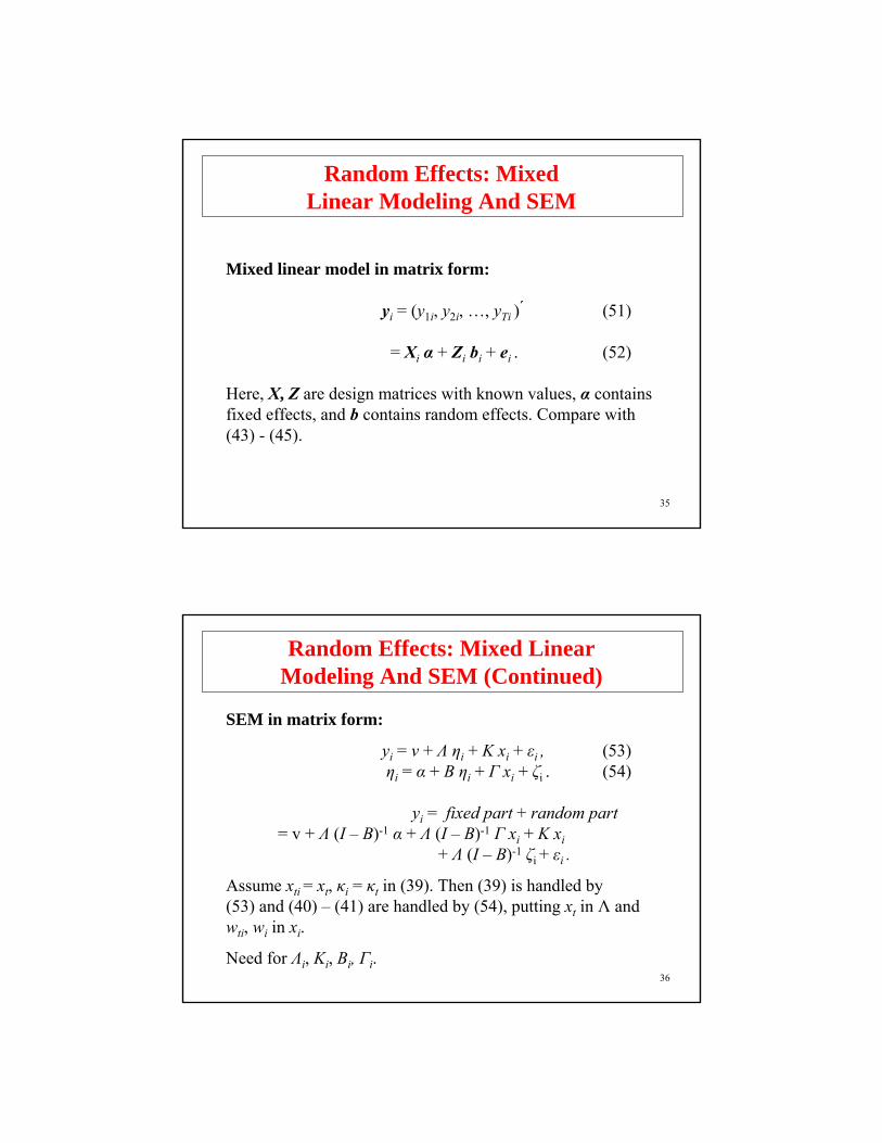
Random Effects: SEM AndMultilevel Modeling (Continued)
SEM approach:
• xt as parameters: Flexible growth function form• Slopes for time-varying covariates vary over time points
Structural part (same as level 2, except for κt):
η0i = α0 + γ0 wi + ζ0i , (48)
η1i = α1 + γ1 wi + ζ1i , (49)
κt not involved (parameter).
35
Random Effects: MixedLinear Modeling And SEM
Mixed linear model in matrix form:
yi = (y1i, y2i, …, yTi ) ́ (51)
= Xi α + Zi bi + ei . (52)
Here, X, Z are design matrices with known values, α containsfixed effects, and b contains random effects. Compare with (43) - (45).
36
Random Effects: Mixed Linear Modeling And SEM (Continued)
SEM in matrix form:
yi = v + Λ ηi + Κ xi + εi , (53)ηi = α + Β ηi + Γ xi + ζi . (54)
yi = fixed part + random part= v + Λ (Ι – Β)-1 α + Λ (Ι – Β)-1 Γ xi + Κ xi
+ Λ (Ι – Β)-1 ζi + εi .
Assume xti = xt, κi = κt in (39). Then (39) is handled by(53) and (40) – (41) are handled by (54), putting xt in Λ andwti, wi in xi.
Need for Λi, Κi, Βi, Γi.

37
yti = ii + six timeti + εti
ii regressed on wisi regressed on wi
• Wide: Multivariate, Single-Level Approach
• Long: Univariate, 2-Level Approach (CLUSTER = id)Within Between
time ys i
Growth Modeling Approached In Two Ways:Data Arranged As Wide Versus Long
y
i s
w
w
i
s
The intercept i is called y in Mplus
Pros And Cons Of Wide Versus Long
• Advantages of the wide approach:– Modeling flexibility
• Unequal residual variances and covariances• Testing of measurement invariance with multiple
indicator growth• Allowing partial measurement non-invariance
– Missing data modeling– Reduction of the number of levels by one (or more)
• Advantages of the long approach – Many time points– Individually-varying times of observation with missingness
38
39
Advantages Of Growth Modeling In A Latent Variable Framework
• Flexible curve shape• Individually-varying times of observation• Regressions among random effects• Multiple processes• Modeling of zeroes• Multiple populations• Multiple indicators• Embedded growth models• Categorical latent variables: growth mixtures
40
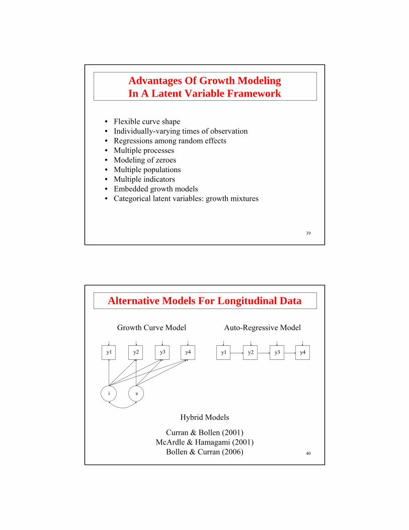
Alternative Models For Longitudinal Data
y1 y2 y3 y4
i s
Growth Curve Model
y1 y2 y3 y4
Auto-Regressive Model
Hybrid Models
Curran & Bollen (2001)McArdle & Hamagami (2001)
Bollen & Curran (2006)

41
The Latent Variable Growth Model In Practice
42
Individual Development Over Time
(1) yti = η0i + η1i xt + εti
(2a) η0i = α0 + γ0 wi + ζ0i
(2b) η1i = α1 + γ1 wi + ζ1i
y1
w
y2 y3 y4
η0 η1
ε1 ε2 ε3 ε4
t = 1 t = 2 t = 3 t = 4
i = 1
i = 2
i = 3
y
x

43
Specifying Time Scores ForLinear Growth Models
Linear Growth Model
• Need two latent variables to describe a linear growth model: Intercept and slope
• Equidistant time scores 0 1 2 3for slope: 0 .1 .2 .3
1 2 3 4
Out
com
e
Time
or
44
Specifying Time Scores ForLinear Growth Models (Continued)
• Nonequidistant time scores 0 1 4 5 6for slope: 0 .1 .4 .5 .6
1 2 3 4 5 6 7
Out
com
e
Time
or
45
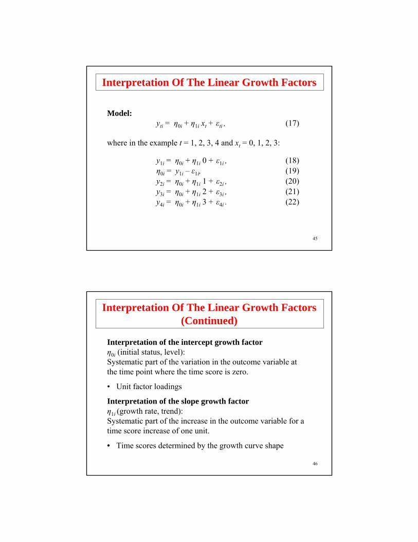
Interpretation Of The Linear Growth Factors
Model:yti = η0i + η1i xt + εti , (17)
where in the example t = 1, 2, 3, 4 and xt = 0, 1, 2, 3:
y1i = η0i + η1i 0 + ε1i , (18)η0i = y1i – ε1i, (19)y2i = η0i + η1i 1 + ε2i , (20)y3i = η0i + η1i 2 + ε3i , (21)y4i = η0i + η1i 3 + ε4i . (22)
46
Interpretation Of The Linear Growth Factors (Continued)
Interpretation of the intercept growth factorη0i (initial status, level):Systematic part of the variation in the outcome variable atthe time point where the time score is zero.
• Unit factor loadings
Interpretation of the slope growth factorη1i (growth rate, trend):Systematic part of the increase in the outcome variable for atime score increase of one unit.
• Time scores determined by the growth curve shape

47
Interpreting Growth Model Parameters
• Intercept Growth Factor Parameters• Mean
• Average of the outcome over individuals at the timepoint with the time score of zero;
• When the first time score is zero, it is the intercept of the average growth curve, also called initial status
• Variance• Variance of the outcome over individuals at the
timepoint with the time score of zero, excluding the residual variance
48
Interpreting Growth Model Parameters (Continued)
• Linear Slope Growth Factor Parameters• Mean – average growth rate over individuals• Variance – variance of the growth rate over individuals
• Covariance with Intercept – relationship between individual intercept and slope values
• Outcome Parameters• Intercepts – not estimated in the growth model – fixed
at zero to represent measurement invariance• Residual Variances – time-specific and measurement
error variation• Residual Covariances – relationships between time-
specific and measurement error sources of variation across time
49
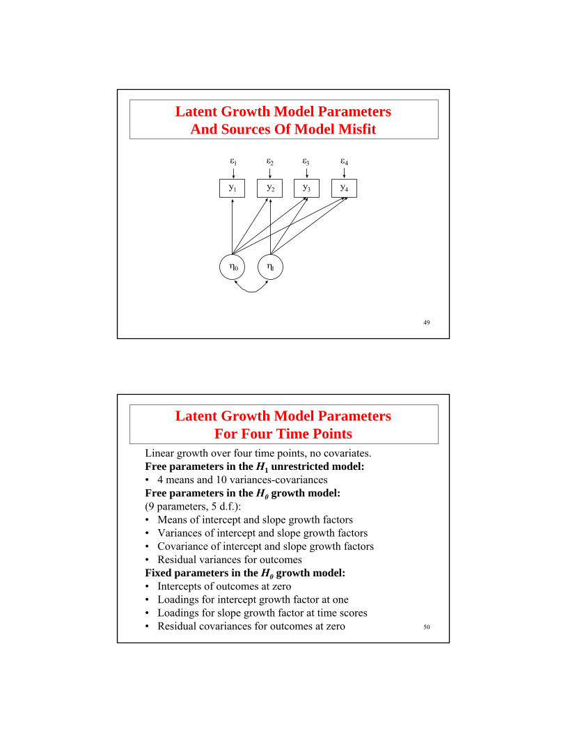
Latent Growth Model ParametersAnd Sources Of Model Misfit
y1 y2 y3 y4
η0 η1
ε1 ε2 ε3 ε4
50
Latent Growth Model ParametersFor Four Time Points
Linear growth over four time points, no covariates.Free parameters in the H1 unrestricted model:• 4 means and 10 variances-covariancesFree parameters in the H0 growth model:(9 parameters, 5 d.f.):• Means of intercept and slope growth factors• Variances of intercept and slope growth factors• Covariance of intercept and slope growth factors• Residual variances for outcomesFixed parameters in the H0 growth model:• Intercepts of outcomes at zero• Loadings for intercept growth factor at one• Loadings for slope growth factor at time scores• Residual covariances for outcomes at zero

51
Latent Growth Model Sources Of Misfit
Sources of misfit:• Time scores for slope growth factor• Residual covariances for outcomes• Outcome variable intercepts• Loadings for intercept growth factor
Model modifications:• Recommended
– Time scores for slope growth factor– Residual covariances for outcomes
• Not recommended– Outcome variable intercepts– Loadings for intercept growth factor
52
Latent Growth Model Parameters For Three Time Points
Linear growth over three time points, no covariates.Free parameters in the H1 unrestricted model:• 3 means and 6 variances-covariancesFree parameters in the H0 growth model(8 parameters, 1 d.f.)• Means of intercept and slope growth factors• Variances of intercept and slope growth factors• Covariance of intercept and slope growth factors• Residual variances for outcomesFixed parameters in the H0 growth model:• Intercepts of outcomes at zero• Loadings for intercept growth factor at one• Loadings for slope growth factor at time scores• Residual covariances for outcomes at zero

53
Growth Model Means And Variancesyti = η0i + η1i xt + εti ,
xt = 0, 1, …, T – 1.
Expectation (mean; E) and variance (V):
E (yti) = E (η0i ) + E (η1i) xt ,V (yti) = V (η0i ) + V (η1i) xt
+ 2xt Cov (η0i , η1i) + V (εti)
V(εti) constant over tCov(η0 , η1) = 0
E(yti)
t0 1 2 3 4
} E(η1i)
}E(η0i)
V(yti)
t0 1 2 3 4
} V(η1i)
}V(η0i)
2
54
Growth Model Covariancesyti = η0i + η1i xt + εti ,xt = 0, 1, …, T – 1.
Cov(yti ,yt ́i ) = V(η0i) + V(η1i) xt xt ́+ Cov(η0i , η1i) (xt + xt ́)+ Cov(εti , εt ́i ).
t
η0 η1
V(η1i ) xt xt :
t
t
η0 η1
Cov(η0i , η1i) xt :
t t
η0 η1
Cov(η0i , η1i) xt :
t
t
η0 η1
V(η0t ) :
t

55
Growth Model Estimation, Testing, AndModel Modification
56
Growth Model Estimation, Testing, AndModel Modification
• Estimation: Model parameters– Maximum-likelihood (ML) estimation under normality– ML and non-normality robust s.e.’s– Quasi-ML (MUML): clustered data (multilevel)– WLS: categorical outcomes– ML-EM: missing data, mixtures
• Model Testing– Likelihood-ratio chi-square testing; robust chi square– Root mean square of approximation (RMSEA):
Close fit (≤ .05)• Model Modification
– Expected drop in chi-square, EPC• Estimation: Individual growth factor values (factor scores)
– Regression method – Bayes modal – Empirical Bayes– Factor determinacy
57
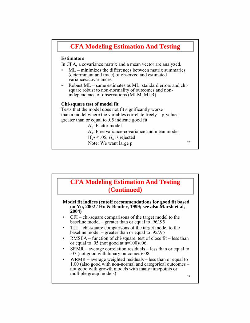
EstimatorsIn CFA, a covariance matrix and a mean vector are analyzed.• ML – minimizes the differences between matrix summaries
(determinant and trace) of observed and estimated variances/covariances
• Robust ML – same estimates as ML, standard errors and chi-square robust to non-normality of outcomes and non-independence of observations (MLM, MLR)
Chi-square test of model fitTests that the model does not fit significantly worse than a model where the variables correlate freely – p-values greater than or equal to .05 indicate good fit
H0: Factor modelH1: Free variance-covariance and mean modelIf p < .05, H0 is rejectedNote: We want large p
CFA Modeling Estimation And Testing
58
Model fit indices (cutoff recommendations for good fit based on Yu, 2002 / Hu & Bentler, 1999; see also Marsh et al, 2004)
• CFI – chi-square comparisons of the target model to the baseline model – greater than or equal to .96/.95
• TLI – chi-square comparisons of the target model to the baseline model – greater than or equal to .95/.95
• RMSEA – function of chi-square, test of close fit – less than or equal to .05 (not good at n=100)/.06
• SRMR – average correlation residuals – less than or equal to .07 (not good with binary outcomes)/.08
• WRMR – average weighted residuals – less than or equal to 1.00 (also good with non-normal and categorical outcomes –not good with growth models with many timepoints or multiple group models)
CFA Modeling Estimation And Testing (Continued)
59
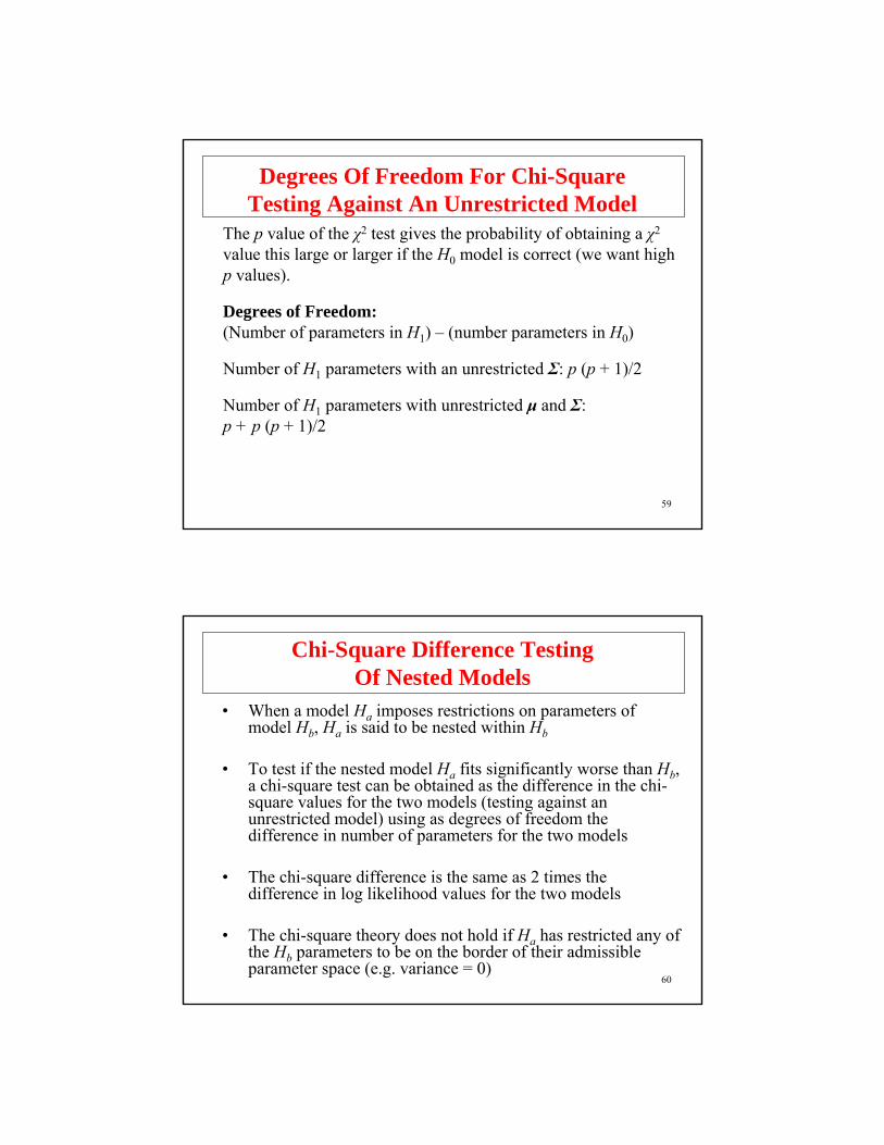
The p value of the χ2 test gives the probability of obtaining a χ2
value this large or larger if the H0 model is correct (we want highp values).
Degrees of Freedom:(Number of parameters in H1) – (number parameters in H0)
Number of H1 parameters with an unrestricted Σ: p (p + 1)/2
Number of H1 parameters with unrestricted μ and Σ: p + p (p + 1)/2
Degrees Of Freedom For Chi-Square Testing Against An Unrestricted Model
60
• When a model Ha imposes restrictions on parameters of model Hb, Ha is said to be nested within Hb
• To test if the nested model Ha fits significantly worse than Hb, a chi-square test can be obtained as the difference in the chi-square values for the two models (testing against an unrestricted model) using as degrees of freedom the difference in number of parameters for the two models
• The chi-square difference is the same as 2 times the difference in log likelihood values for the two models
• The chi-square theory does not hold if Ha has restricted any of the Hb parameters to be on the border of their admissible parameter space (e.g. variance = 0)
Chi-Square Difference Testing Of Nested Models

61
CFA Model Modification
Model modification indices are estimated for all parameters thatare fixed or constrained to be equal.
• Modification Indices – expected drop in chi-square if the parameter is estimated
• Expected Parameter Change Indices – expected value of the parameter if it is estimated
• Standardized Expected Parameter Change Indices –standardized expected value of the parameter if it is estimated
Model Modifications
• Residual covariances• Factor cross loadings
62
Alternative Growth Model Parameterizations
Parameterization 1 – for continuous outcomes
yti = 0 + η0i + η1i xt + εti , (32)η0i = α0 + ζ0i , (33)η1i = α1 + ζ1i . (34)
Parameterization 2 – for categorical outcomes andmultiple indicators
yti = v + η0i + η1i xt + εti , (35)η0i = 0 + ζ0i , (36)η1i = α1 + ζ1i . (37)
63
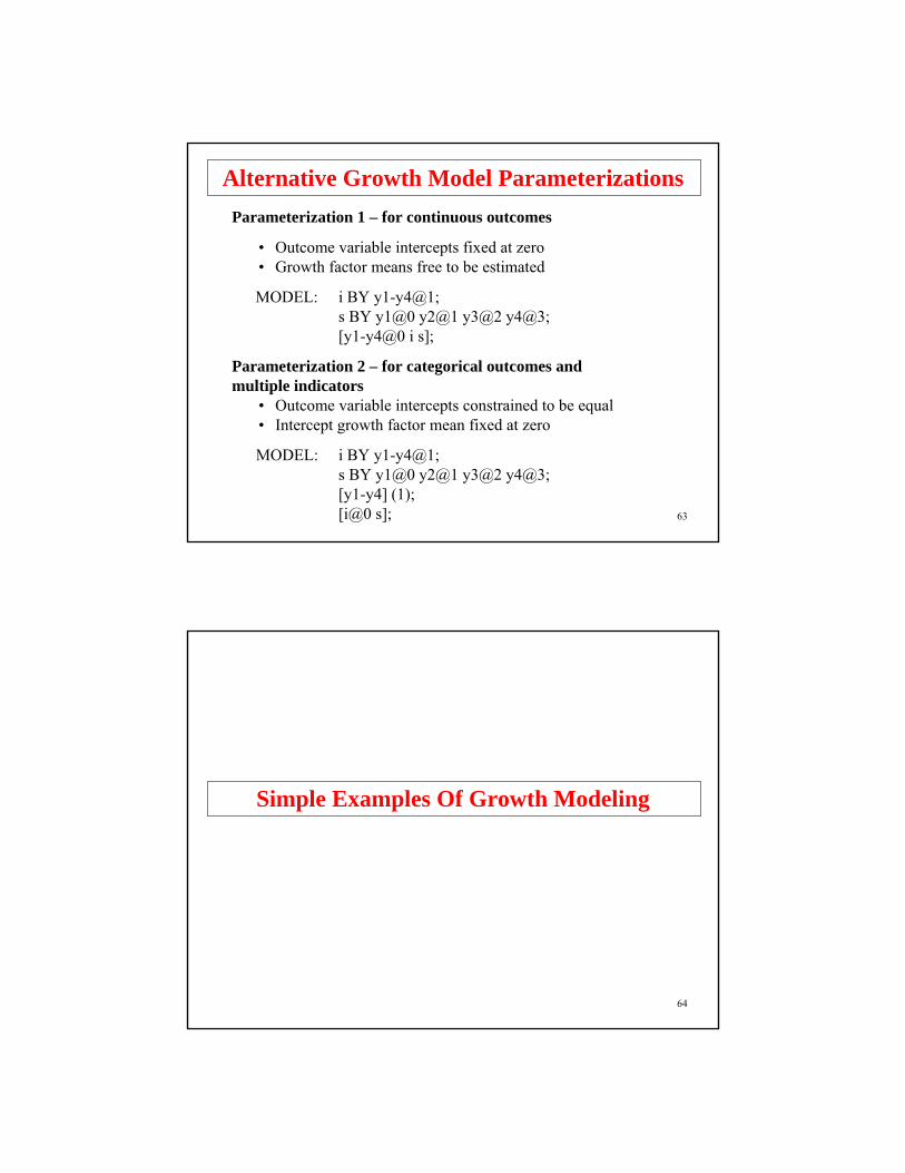
Alternative Growth Model ParameterizationsParameterization 1 – for continuous outcomes
• Outcome variable intercepts fixed at zero• Growth factor means free to be estimated
MODEL: i BY y1-y4@1;s BY y1@0 y2@1 y3@2 y4@3;[y1-y4@0 i s];
Parameterization 2 – for categorical outcomes andmultiple indicators
• Outcome variable intercepts constrained to be equal• Intercept growth factor mean fixed at zero
MODEL: i BY y1-y4@1;s BY y1@0 y2@1 y3@2 y4@3;[y1-y4] (1);[i@0 s];
64
Simple Examples Of Growth Modeling

65
Steps In Growth Modeling• Preliminary descriptive studies of the data: means,
variances, correlations, univariate and bivariate distributions, outliers, etc.
• Determine the shape of the growth curve from theory and/or data
• Individual plots
• Mean plot
• Consider change in variance across time
• Fit model without covariates using fixed time scores
• Modify model as needed
• Add covariates
66Grade
Mat
h A
chie
vem
ent
7 8 9 10
4050
6070
80
7 8 9 10
Mat
h A
chie
vem
ent
Grade
Individual Curves
4050
6070
80
Mean Curve
LSAY Math Achievement
67
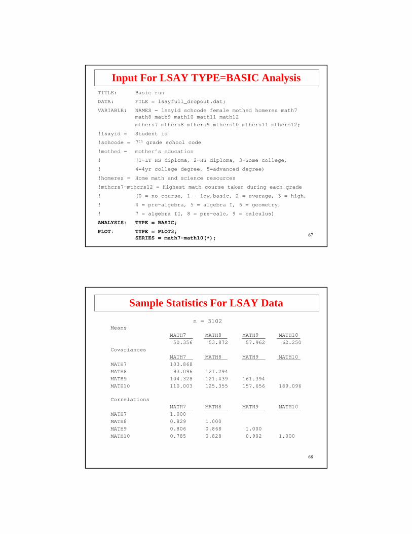
Input For LSAY TYPE=BASIC AnalysisTITLE: Basic run
DATA: FILE = lsayfull_dropout.dat;
VARIABLE: NAMES = lsayid schcode female mothed homeres math7 math8 math9 math10 math11 math12 mthcrs7 mthcrs8 mthcrs9 mthcrs10 mthcrs11 mthcrs12;
!lsayid = Student id
!schcode = 7th grade school code
!mothed = mother’s education
! (1=LT HS diploma, 2=HS diploma, 3=Some college,
! 4=4yr college degree, 5=advanced degree)
!homeres = Home math and science resources
!mthcrs7-mthcrs12 = Highest math course taken during each grade
! (0 = no course, 1 – low,basic, 2 = average, 3 = high,
! 4 = pre-algebra, 5 = algebra I, 6 = geometry,
! 7 = algebra II, 8 = pre-calc, 9 = calculus)
ANALYSIS: TYPE = BASIC;
PLOT: TYPE = PLOT3; SERIES = math7-math10(*);
68
Sample Statistics For LSAY Datan = 3102
MeansMATH7 MATH8 MATH9 MATH1050.356 53.872 57.962 62.250
CovariancesMATH7 MATH8 MATH9 MATH10
MATH7 103.868MATH8 93.096 121.294MATH9 104.328 121.439 161.394MATH10 110.003 125.355 157.656 189.096
CorrelationsMATH7 MATH8 MATH9 MATH10
MATH7 1.000MATH8 0.829 1.000MATH9 0.806 0.868 1.000MATH10 0.785 0.828 0.902 1.000

69
math7 math8 math9 math10
i s
70
TITLE: Growth 7 – 10, no covariates
DATA: FILE = lsayfull_dropout.dat;
VARIABLE: NAMES = lsayid schcode female mothed homeres
math7 math8 math9 math10 math11 math12
mthcrs7 mthcrs8 mthcrs9 mthcrs10 mthcrs11 mthcrs12;
USEV = math7-math10;
MISSING = ALL(9999);
MODEL: i BY math7-math10@1;
s BY math7@0 math8@1 math9@2 math10@3;
[math7-math10@0];[i s];
OUTPUT: SAMPSTAT STANDARDIZED RESIDUAL MODINDICES (3.84);
Alternative language:
MODEL: i s | math7@0 math8@1 math9@2 math10@3;
Input For LSAY Linear Growth ModelWithout Covariates
71
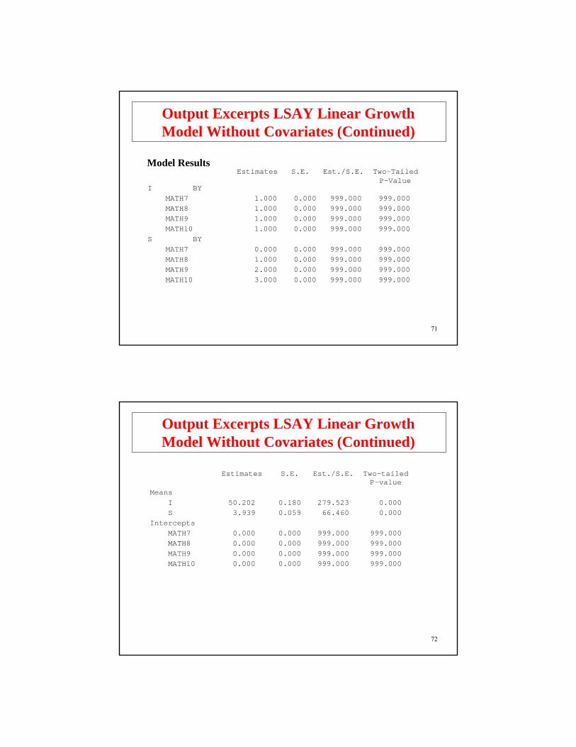
I BYMATH7 1.000 0.000 999.000 999.000MATH8 1.000 0.000 999.000 999.000MATH9 1.000 0.000 999.000 999.000MATH10 1.000 0.000 999.000 999.000
S BYMATH7 0.000 0.000 999.000 999.000MATH8 1.000 0.000 999.000 999.000MATH9 2.000 0.000 999.000 999.000MATH10 3.000 0.000 999.000 999.000
Estimates S.E. Est./S.E. Two-TailedP-Value
Model Results
Output Excerpts LSAY Linear GrowthModel Without Covariates (Continued)
72
Output Excerpts LSAY Linear GrowthModel Without Covariates (Continued)
Estimates S.E. Est./S.E. Two-tailedP-value
MeansI 50.202 0.180 279.523 0.000S 3.939 0.059 66.460 0.000
InterceptsMATH7 0.000 0.000 999.000 999.000MATH8 0.000 0.000 999.000 999.000MATH9 0.000 0.000 999.000 999.000MATH10 0.000 0.000 999.000 999.000

73
Observed Variable R-Square
MATH7 0.832MATH8 0.853MATH9 0.895MATH10 0.912
R-Square
Output Excerpts LSAY Linear GrowthModel Without Covariates (Continued)
Estimates S.E. Est./S.E. Two-tailedP-value
Residual VariancesMATH7 17.430 1.002 17.400 0.000MATH8 18.440 0.750 24.596 0.000MATH9 16.184 0.757 20.561 0.000MATH10 17.219 1.301 13.230 0.000
VariancesI 86.159 2.606 33.067 0.000S 4.792 0.295 16.262 0.000
I WITHS 8.031 0.654 12.276 0.000
74
Tests Of Model Fit
Chi-Square Test of Model FitValue 86.541Degrees of Freedom 5P-Value 0.0000
CFI/TLICFI 0.992TLI 0.990
RMSEA (Root Mean Square Error Of Approximation)Estimate 0.07390 Percent C.I. 0.060 0.086Probability RMSEA <= .05 0.002
SRMR (Standardized Root Mean Square Residual)Value 0.047
Output Excerpts LSAY Linear GrowthModel Without Covariates (Continued)
75
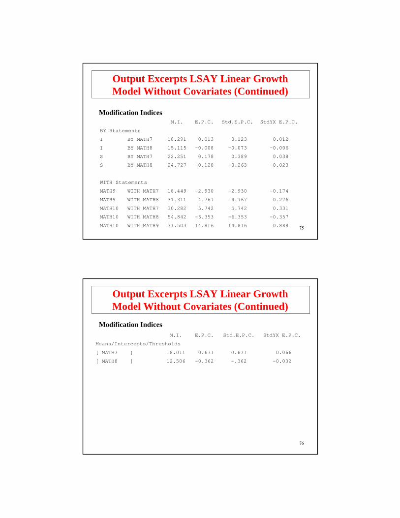
M.I. E.P.C. Std.E.P.C. StdYX E.P.C.
BY Statements
I BY MATH7 18.291 0.013 0.123 0.012
I BY MATH8 15.115 -0.008 -0.073 -0.006
S BY MATH7 22.251 0.178 0.389 0.038
S BY MATH8 24.727 -0.120 -0.263 -0.023
WITH Statements
MATH9 WITH MATH7 18.449 -2.930 -2.930 -0.174
MATH9 WITH MATH8 31.311 4.767 4.767 0.276
MATH10 WITH MATH7 30.282 5.742 5.742 0.331
MATH10 WITH MATH8 54.842 -6.353 -6.353 -0.357
MATH10 WITH MATH9 31.503 14.816 14.816 0.888
Modification Indices
Output Excerpts LSAY Linear GrowthModel Without Covariates (Continued)
76
M.I. E.P.C. Std.E.P.C. StdYX E.P.C.
Means/Intercepts/Thresholds
[ MATH7 ] 18.011 0.671 0.671 0.066
[ MATH8 ] 12.506 -0.362 -.362 -0.032
Output Excerpts LSAY Linear GrowthModel Without Covariates (Continued)
Modification Indices
77
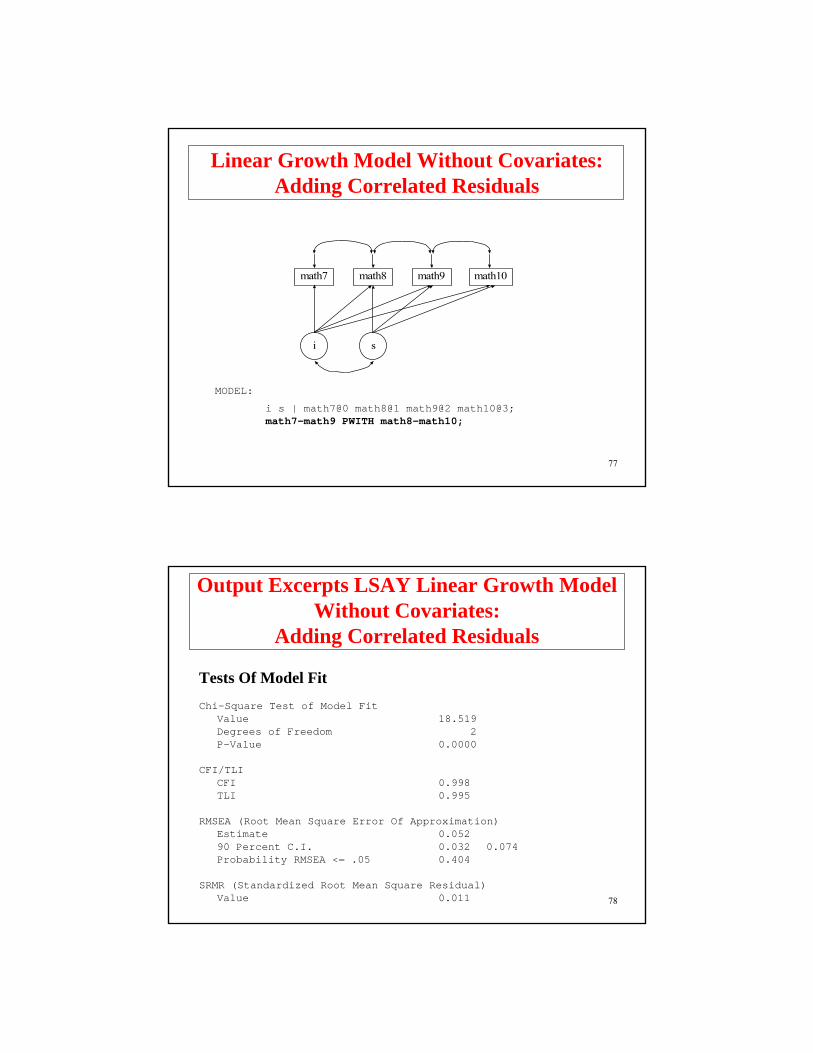
Linear Growth Model Without Covariates: Adding Correlated Residuals
MODEL:
i s | math7@0 math8@1 math9@2 math10@3;math7-math9 PWITH math8-math10;
math7 math8 math9 math10
i s
78
Output Excerpts LSAY Linear Growth Model Without Covariates:
Adding Correlated Residuals
Tests Of Model FitChi-Square Test of Model Fit
Value 18.519Degrees of Freedom 2P-Value 0.0000
CFI/TLICFI 0.998TLI 0.995
RMSEA (Root Mean Square Error Of Approximation)Estimate 0.05290 Percent C.I. 0.032 0.074Probability RMSEA <= .05 0.404
SRMR (Standardized Root Mean Square Residual)Value 0.011

79
Output Excerpts LSAY: Adding Correlated Residuals (Continued)
Estimates S.E. Est./S.E. Two-tailedP-value
S WITHI 6.133 1.379 4.447 0.000
MATH7 WITHMATH8 -5.078 2.146 -2.366 0.018
MATH8 WITHMATH9 4.917 0.916 5.365 0.000
MATH9 WITHMATH10 17.062 2.983 5.720 0.000
MeansI 50.203 0.180 279.431 0.000S 3.936 0.059 66.693 0.000
80
Estimates S.E. Est./S.E. Two-tailedP-value
Variances
I 92.038 4.167 22.085 0.000
S 3.043 0.789 3.858 0.000
Residual Variances
MATH7 11.871 3.466 3.425 0.001
MATH8 14.027 1.980 7.085 0.000
MATH9 32.596 2.609 12.492 0.000
MATH10 33.857 4.815 7.032 0.000
Output Excerpts LSAY: Adding Correlated Residuals (Continued)

81
ESTIMATED MODEL AND RESIDUALS (OBSERVED – ESTIMATED)
Model Estimated Means/Intercepts/Thresholds
MATH7 MATH8 MATH9 MATH10
1 50.203 54.140 58.076 62.012
Residuals for Means/Intercepts/Thresholds
MATH7 MATH8 MATH9 MATH10
1 0.153 -0.267 -0.114 0.238
Standardized Residuals (z-scores) for Means/Intercepts/Thresholds
MATH7 MATH8 MATH9 MATH10
1 4.198 -4.109 -1.256 5.199
Normalized Residuals for Means/Intercepts/Thresholds
MATH7 MATH8 MATH9 MATH10
1 0.834 -1.317 -0.478 0.904
Output Excerpts LSAY: Adding Correlated Residuals (Continued)
82
Model Estimated Covariances/Correlations/Residual Correlations
MATH7 MATH8 MATH9 MATH10
MATH7 103.910
MATH8 93.093 121.375
MATH9 104.304 121.441 161.339
MATH10 110.437 125.700 158.025 190.083
Residuals for Covariances/Correlations/Residual Correlations
MATH7 MATH8 MATH9 MATH10
MATH7 -0.041
MATH8 0.002 -0.081
MATH9 0.024 -0.002 0.055
MATH10 -0.434 -0.345 -0.368 -0.987
Output Excerpts LSAY:Adding Correlated Residuals (Continued)
83
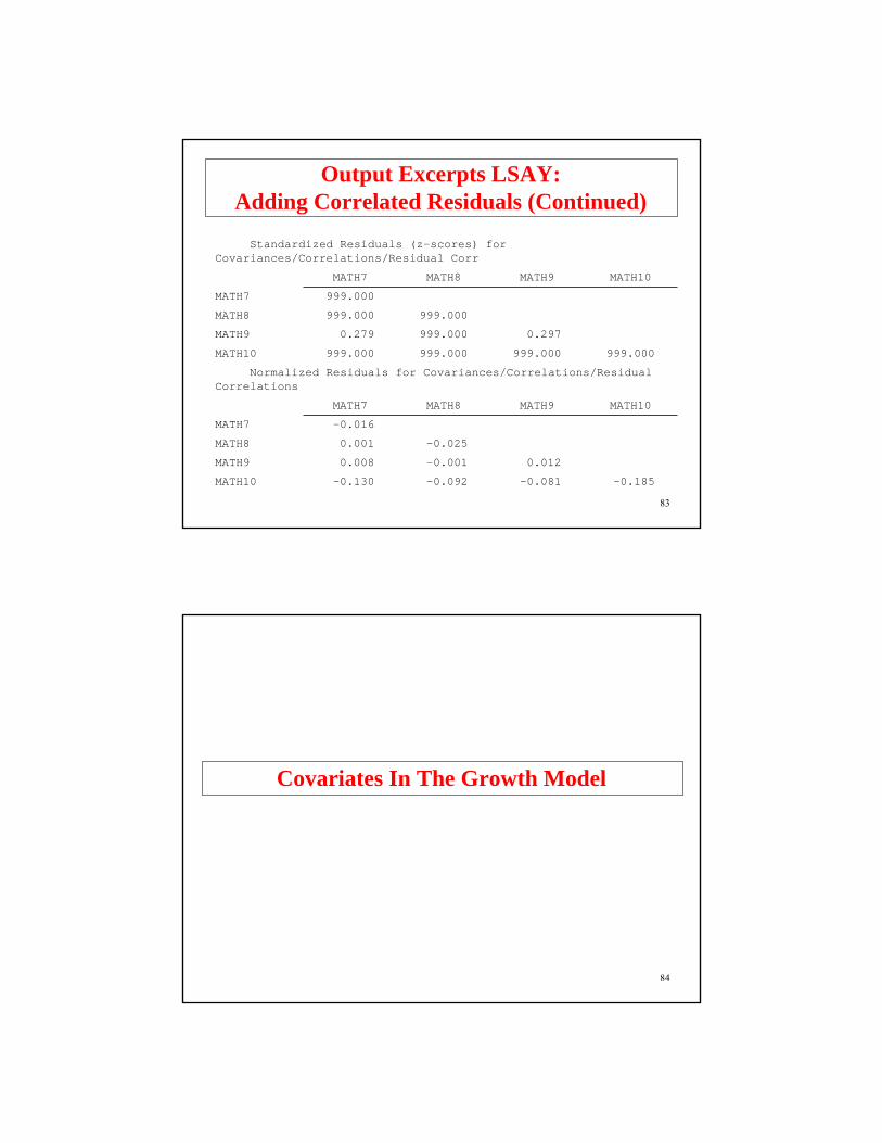
Output Excerpts LSAY: Adding Correlated Residuals (Continued)
Standardized Residuals (z-scores) for Covariances/Correlations/Residual Corr
MATH7 MATH8 MATH9 MATH10
MATH7 999.000
MATH8 999.000 999.000
MATH9 0.279 999.000 0.297
MATH10 999.000 999.000 999.000 999.000
Normalized Residuals for Covariances/Correlations/Residual Correlations
MATH7 MATH8 MATH9 MATH10
MATH7 -0.016
MATH8 0.001 -0.025
MATH9 0.008 -0.001 0.012
MATH10 -0.130 -0.092 -0.081 -0.185
84
Covariates In The Growth Model

85
• Types of covariates
• Time-invariant covariates—vary across individuals not time, explain the variation in the growth factors
• Time-varying covariates—vary across individuals and time, explain the variation in the outcomes beyond the growth factors
Covariates In The Growth Model
86
y1 y2 y3 y4
η0
η1
w a21 a22 a23 a24
Time-Invariant AndTime-Varying Covariates

87
LSAY Growth Model With Time-Invariant Covariates
math7 math8 math9 math10
i s
mothed homeresfemale
88
Input Excerpts For LSAY Linear Growth Model With Time-Invariant Covariates
TITLE: Growth 7 – 10, no covariates
DATA: FILE = lsayfull_dropout.dat;
VARIABLE: NAMES = lsayid schcode female mothed homeres math7 math8 math9 math10 math11 math12
mthcrs7 mthcrs8 mthcrs9 mthcrs10 mthcrs11 mthcrs12;
MISSING = ALL (999);USEVAR = math7-math10 female mothed homeres;
ANALYSIS: !ESTIMATOR = MLR;
MODEL: i s | math7@0 math8@1 math9@2 math10@3;i s ON female mothed homeres;
Alternative language:
MODEL: i BY math7-math10@1;s BY math7@0 math8@1 math9@2 math10@3;[math7-math10@0];[i s];i s ON female mothed homeres;
89
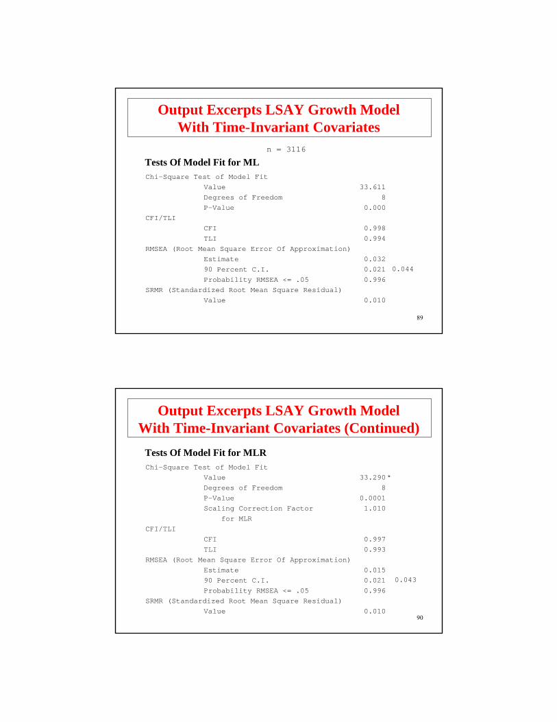
Output Excerpts LSAY Growth ModelWith Time-Invariant Covariates
Chi-Square Test of Model FitValue 33.611Degrees of Freedom 8P-Value 0.000
CFI/TLICFI 0.998TLI 0.994
RMSEA (Root Mean Square Error Of Approximation)Estimate 0.03290 Percent C.I. 0.021Probability RMSEA <= .05 0.996
SRMR (Standardized Root Mean Square Residual)Value 0.010
Tests Of Model Fit for MLn = 3116
0.044
90
Output Excerpts LSAY Growth ModelWith Time-Invariant Covariates (Continued)
Tests Of Model Fit for MLRChi-Square Test of Model Fit
Value 33.290Degrees of Freedom 8P-Value 0.0001Scaling Correction Factor 1.010
for MLRCFI/TLI
CFI 0.997TLI 0.993
RMSEA (Root Mean Square Error Of Approximation)Estimate 0.01590 Percent C.I. 0.021Probability RMSEA <= .05 0.996
SRMR (Standardized Root Mean Square Residual)Value 0.010
*
0.043
91
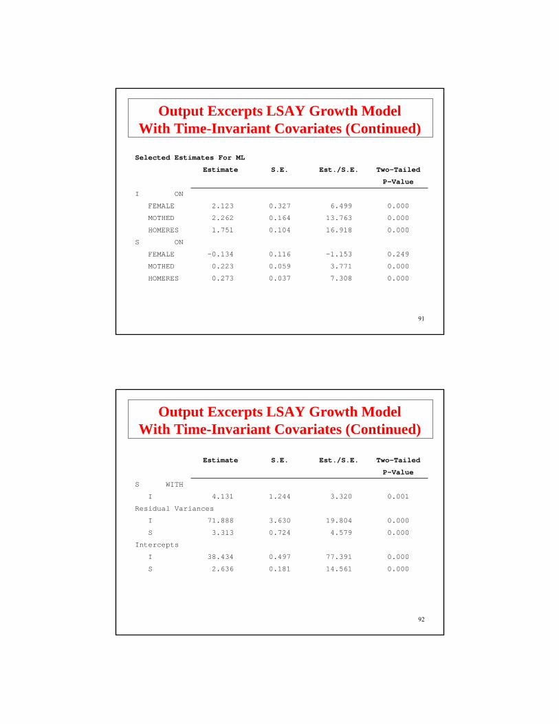
Selected Estimates For ML
Estimate S.E. Est./S.E. Two-Tailed
P-Value
I ON
FEMALE 2.123 0.327 6.499 0.000
MOTHED 2.262 0.164 13.763 0.000
HOMERES 1.751 0.104 16.918 0.000
S ON
FEMALE -0.134 0.116 -1.153 0.249
MOTHED 0.223 0.059 3.771 0.000
HOMERES 0.273 0.037 7.308 0.000
Output Excerpts LSAY Growth ModelWith Time-Invariant Covariates (Continued)
92
Estimate S.E. Est./S.E. Two-Tailed
P-Value
S WITH
I 4.131 1.244 3.320 0.001
Residual Variances
I 71.888 3.630 19.804 0.000
S 3.313 0.724 4.579 0.000
Intercepts
I 38.434 0.497 77.391 0.000
S 2.636 0.181 14.561 0.000
Output Excerpts LSAY Growth ModelWith Time-Invariant Covariates (Continued)

93
Observed Variable R-Square
MATH7 0.876MATH8 0.863MATH9 0.817MATH10 0.854
LatentVariable R-Square
I .204S .091
R-Square
Output Excerpts LSAY Growth ModelWith Time-Invariant Covariates (Continued)
94
Output Excerpts LSAY Growth ModelWith Time-Invariant Covariates (Continued)TECHNICAL 4 OUTPUT
ESTIMATES DERIVED FROM THE MODEL
ESTIMATED MEANS FOR THE LATENT VARIABLES
I S FEMALE MOTHED HOMERES
50.219 3.944 0.478 2.347 3.118
95
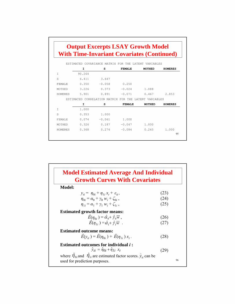
ESTIMATED COVARIANCE MATRIX FOR THE LATENT VARIABLES
I S FEMALE MOTHED HOMERES
I 90.264
S 6.411 3.647
FEMALE 0.350 -0.058 0.250
MOTHED 3.226 0.373 -0.024 1.088
HOMERES 5.901 0.891 -0.071 0.467 2.853
ESTIMATED CORRELATION MATRIX FOR THE LATENT VARIABLES
I S FEMALE MOTHED HOMERES
I 1.000
S 0.353 1.000
FEMALE 0.074 -0.061 1.000
MOTHED 0.326 0.187 -0.047 1.000
HOMERES 0.368 0.276 -0.084 0.265 1.000
Output Excerpts LSAY Growth ModelWith Time-Invariant Covariates (Continued)
96
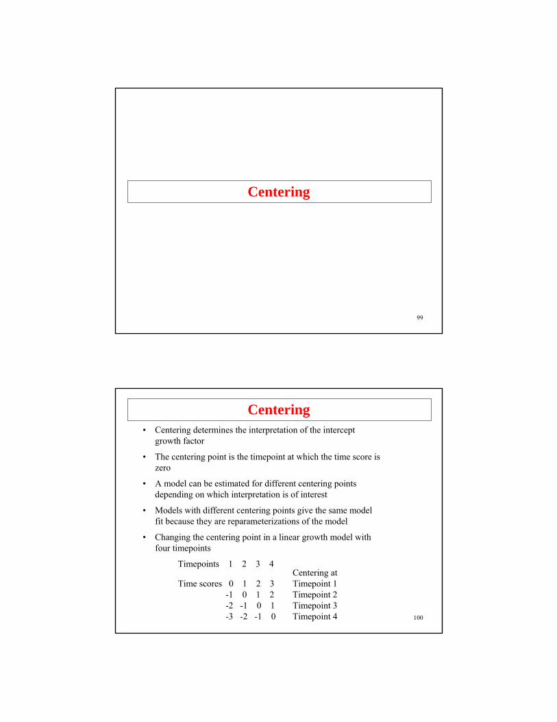
Model Estimated Average And IndividualGrowth Curves With Covariates
Model:yti = η0i + η1i xt + εti , (23)η0i = α0 + γ0 wi + ζ0i , (24)η1i = α1 + γ1 wi + ζ1i , (25)
Estimated growth factor means:Ê(η0i ) = , (26)Ê(η1i ) = . (27)
Estimated outcome means:Ê(yti ) = Ê(η0i ) + Ê(η1i ) xt . (28)
Estimated outcomes for individual i :(29)
where and are estimated factor scores. yti can beused for prediction purposes.
w00 ˆˆ γα +w11 ˆˆ γα +
t1i0iti xηηy ˆˆˆ +=
i0η̂ i1̂η

97
Model Estimated Means With CovariatesModel estimated means are available using the TECH4 and RESIDUAL options of
the OUTPUT command.
Estimated Intercept Mean = Estimated Intercept +Estimated Slope (Female)*Sample Mean (Female) +Estimated Slope (Mothed)*Sample Mean (Mothed) +Estimated Slope (Homeres)*Sample Mean (Homeres)
38.43 + 2.12*0.48 + 2.26*2.35 + 1.75*3.12 = 50.22
Estimated Slope Mean = Estimated Intercept +Estimated Slope (Female)*Sample Mean (Female) + Estimated Slope (Mothed)*Sample Mean (Mothed) +Estimated Slope (Homeres)*Sample Mean (Homeres)
2.64 – 0.13*0.48 + 0.22*2.35 + 0.27*3.11 = 3.94
98
Model Estimated Means With Covariates(Continued)
Estimated Outcome Mean at Timepoint t =
Estimated Intercept Mean +Estimated Slope Mean * (Time Score at Timepoint t)
Estimated Outcome Mean at Timepoint 1 =50.22 + 3.94 * (0) = 50.22
Estimated Outcome Mean at Timepoint 2 =50.22 + 3.94 * (1.00) = 54.16
Estimated Outcome Mean at Timepoint 3 =50.22 + 3.94 * (2.00) = 58.11
Estimated Outcome Mean at Timepoint 4 =50.22 + 3.94 * (3.00) = 62.05
99
Centering
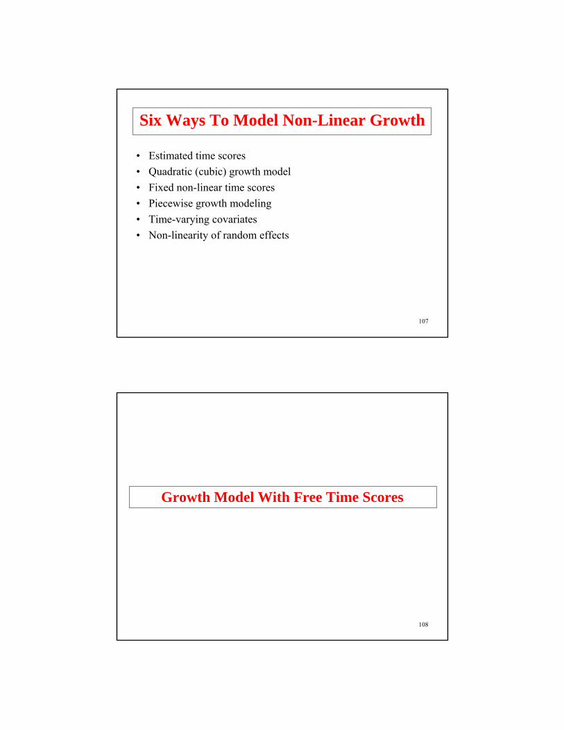
100
Centering• Centering determines the interpretation of the intercept
growth factor
• The centering point is the timepoint at which the time score iszero
• A model can be estimated for different centering pointsdepending on which interpretation is of interest
• Models with different centering points give the same modelfit because they are reparameterizations of the model
• Changing the centering point in a linear growth model withfour timepoints
Timepoints 1 2 3 4Centering at
Time scores 0 1 2 3 Timepoint 1-1 0 1 2 Timepoint 2-2 -1 0 1 Timepoint 3-3 -2 -1 0 Timepoint 4

101
Input Excerpts For LSAY Growth Model With Covariates Centered At Grade 10
MODEL: i s | math7@-3 math8@-2 math9@-1 math10@0;i s ON female mothed homeres;math7-math9 PWITH math8-math10;
OUTPUT: TECH1 RESIDUAL STANDARDIZED MODINDICES TECH4;
Alternative language:
MODEL: i BY math7-math10@1;s BY math7@-3 math8@-2 math9@-1 math10@0;math7-math9 PWITH math8-math10;[math7-math10@0];[i s];i s ON female mothed homeres;
102
n = 3116
Tests of Model Fit
CHI-SQUARE TEST OF MODEL FIT
Value 33.611Degrees of Freedom 8P-Value 0.000
RMSEA (ROOT MEAN SQUARE ERROR OF APPROXIMATION)
Estimate .03290 Percent C.I. .021 .044Probability RMSEA <= .05 .996
Output Excerpts LSAY Growth Model With Covariates Centered At Grade 10

103
Output Excerpts LSAY Growth Model With Covariates Centered At Grade 10
(Continued)SELECTED ESTIMATES
Estimate S.E. Est./S.E. Two-Tailed
P-Value
I ON
FEMALE 1.723 0.473 3.643 0.000
MOTHED 2.930 0.239 12.249 0.000
HOMERES 2.569 0.151 17.002 0.000
S ON
FEMALE -0.133 0.116 -1.153 0.249
MOTHED 0.223 0.059 3.771 0.000
HOMERES 0.273 0.037 7.308 0.000
104
Further Readings On Introductory Growth Modeling
Bijleveld, C. C. J. H., & van der Kamp, T. (1998). Longitudinal data analysis: Designs, models, and methods. Newbury Park: Sage.
Bollen, K.A. & Curran, P.J. (2006). Latent curve models. A structural equation perspective. New York: Wiley.
Duncan, T., Duncan S. & Strycker, L. (2006). An introduction to latent variable growth curve modeling. Second edition. Lawrence Erlbaum: New York.
Muthén, B. & Khoo, S.T. (1998). Longitudinal studies of achievement growth using latent variable modeling. Learning and Individual Differences, Special issue: latent growth curve analysis, 10, 73-101. (#80)
Muthén, B. & Muthén, L. (2000). The development of heavy drinking and alcohol-related problems from ages 18 to 37 in a U.S. national sample. Journal of Studies on Alcohol, 61, 290-300. (#83)

105
Further Readings On Introductory Growth Modeling (Continued)
Raudenbush, S.W. & Bryk, A.S. (2002). Hierarchical linear models: Applications and data analysis methods. Second edition. Newbury Park, CA: Sage Publications.
Singer, J.D. & Willett, J.B. (2003). Applied longitudinal data analysis. Modeling change and event occurrence. New York, NY: Oxford University Press.
Snijders, T. & Bosker, R. (1999). Multilevel analysis. An introduction to basic and advanced multilevel modeling. Thousand Oakes, CA: Sage Publications.
106
Non-Linear Growth
107
Six Ways To Model Non-Linear Growth
• Estimated time scores • Quadratic (cubic) growth model • Fixed non-linear time scores • Piecewise growth modeling• Time-varying covariates • Non-linearity of random effects
108
Growth Model With Free Time Scores

109
Specifying Time Scores For Non-LinearGrowth Models With Estimated Time Scores
Non-linear growth models with estimated time scores
• Need two latent variables to describe a non-linear growth model: Intercept and slope
Time scores: 0 1 Estimated Estimated
1 2 3 4
∗
∗
Out
com
e
Out
com
eTime Time
1 2 3 4
∗∗
110
Input Excerpts For LSAY Linear Growth Model With Free Time Scores
Without Covariates
MODEL: i s | math7@0 math8@1 math9@2 math10@3 math11@4 math12*5;
Alternative language:
MODEL: i BY math7-math12@1;s BY math7@0 math8@1 math9@2 math10@3 math11@4 math12*5;[math7-math12@0];[i s];
111
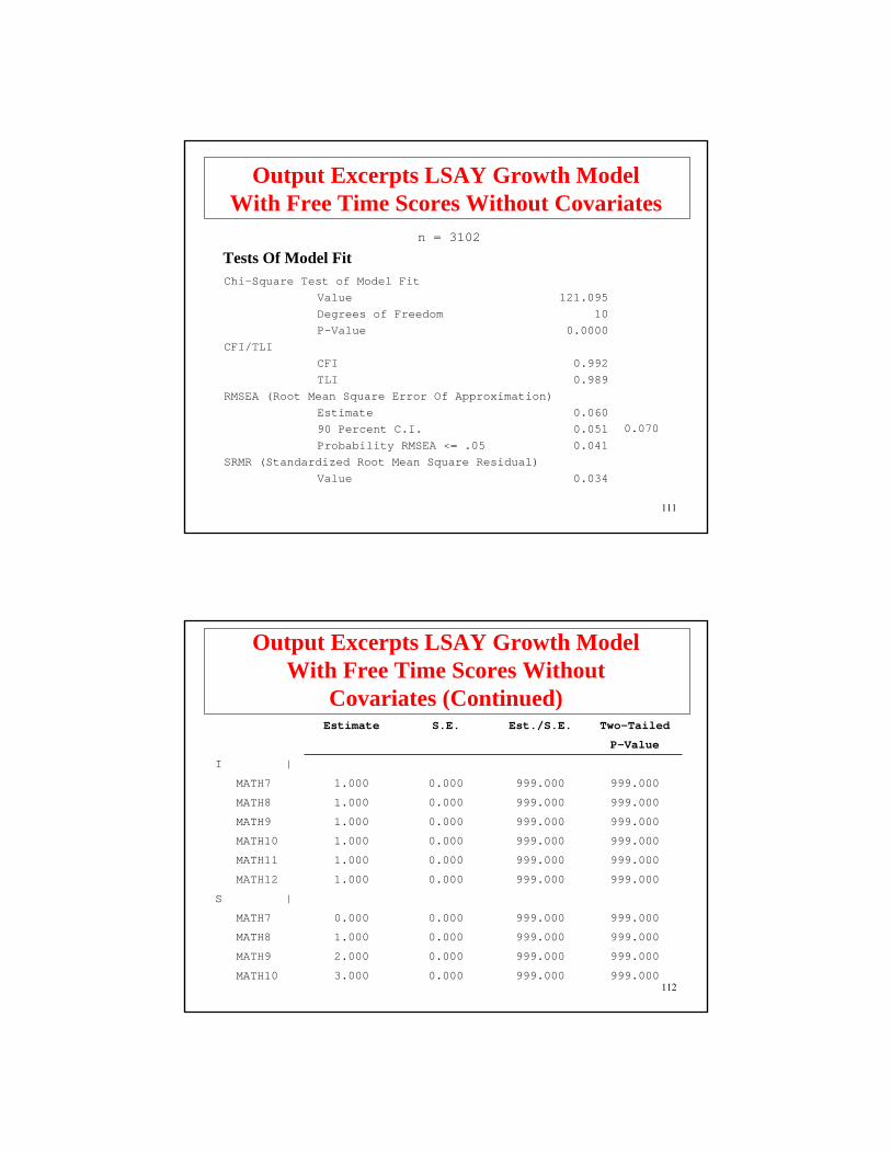
Output Excerpts LSAY Growth ModelWith Free Time Scores Without Covariates
Chi-Square Test of Model FitValue 121.095Degrees of Freedom 10P-Value 0.0000
CFI/TLICFI 0.992TLI 0.989
RMSEA (Root Mean Square Error Of Approximation)Estimate 0.06090 Percent C.I. 0.051Probability RMSEA <= .05 0.041
SRMR (Standardized Root Mean Square Residual)Value 0.034
Tests Of Model Fitn = 3102
0.070
112
Output Excerpts LSAY Growth Model With Free Time Scores Without
Covariates (Continued)Estimate S.E. Est./S.E. Two-Tailed
P-Value
I |
MATH7 1.000 0.000 999.000 999.000
MATH8 1.000 0.000 999.000 999.000
MATH9 1.000 0.000 999.000 999.000
MATH10 1.000 0.000 999.000 999.000
MATH11 1.000 0.000 999.000 999.000
MATH12 1.000 0.000 999.000 999.000
S |
MATH7 0.000 0.000 999.000 999.000
MATH8 1.000 0.000 999.000 999.000
MATH9 2.000 0.000 999.000 999.000
MATH10 3.000 0.000 999.000 999.000

113
Output Excerpts LSAY Growth Model With Free Time Scores Without
Covariates (Continued)
Estimate S.E. Est./S.E. Two-Tailed
P-Value
MATH11 4.000 0.000 999.000 999.000
MATH12 4.095 0.042 97.236 0.000
S WITH
I 4.986 0.741 6.725 0.000
Variances
I 91.374 3.046 29.994 0.000
S 4.001 0.276 14.666 0.000
Means
I 50.323 0.180 279.612 0.000
S 3.752 0.049 76.472 0.000
114
• Identification of the model – for a model with two growth factors, at least one time score must be fixed to a non-zero value (usually one) in addition to the time score that is fixed at zero (centering point)
• Interpretation—cannot interpret the mean of the slope growth factor as a constant rate of change over all timepoints, but as the rate of change for a time score change of one.
• Approach—fix the time score following the centering point at one
Growth Model With Free Time Scores

115
• The slope growth factor mean is the expected change in the outcome variable for a one unit change in the time score
• In non-linear growth models, the time scores should be chosen so that a one unit change occurs between timepoints of substantive interest.
• An example of 4 timepoints representing grades 7, 8, 9, and 10
• Time scores of 0 1 * * – slope factor mean refers to expected change between grades 7 and 8
• Time scores of 0 * * 1 – slope factor mean refers to expected change between grades 7 and 10
Interpretation Of Slope Growth Factor MeanFor Non-Linear Models
116
Specifying Time Scores For Quadratic Growth Models
• Linear slope time scores: 0 1 2 3 or 0 .1 .2 .3• Quadratic slope time scores: 0 1 4 9 or 0 .01 .04 .09
xt2
1 2 3 4
Out
com
e
Time
Quadratic growth model
yti = η0i + η1i xt + η2i + εti or
• Need three latent variables to describe a quadratic growth model: Intercept, linear slope, quadratic slope
where c is a centering constant, e.g.
2t2iti1i0ti )cx()cx(y −⋅+−⋅+= ηηη
x
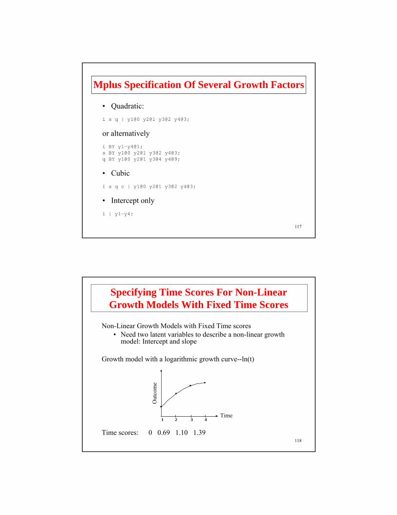
Mplus Specification Of Several Growth Factors
• Quadratic:i s q | y1@0 y2@1 y3@2 y4@3;
or alternativelyi BY y1-y4@1;s BY y1@0 y2@1 y3@2 y4@3;q BY y1@0 y2@1 y3@4 y4@9;
• Cubici s q c | y1@0 y2@1 y3@2 y4@3;
• Intercept onlyi | y1-y4;
117
118
Specifying Time Scores For Non-LinearGrowth Models With Fixed Time Scores
Non-Linear Growth Models with Fixed Time scores• Need two latent variables to describe a non-linear growth
model: Intercept and slope
Growth model with a logarithmic growth curve--ln(t)
Time scores: 0 0.69 1.10 1.39
1 2 3 4
Out
com
e
Time
119
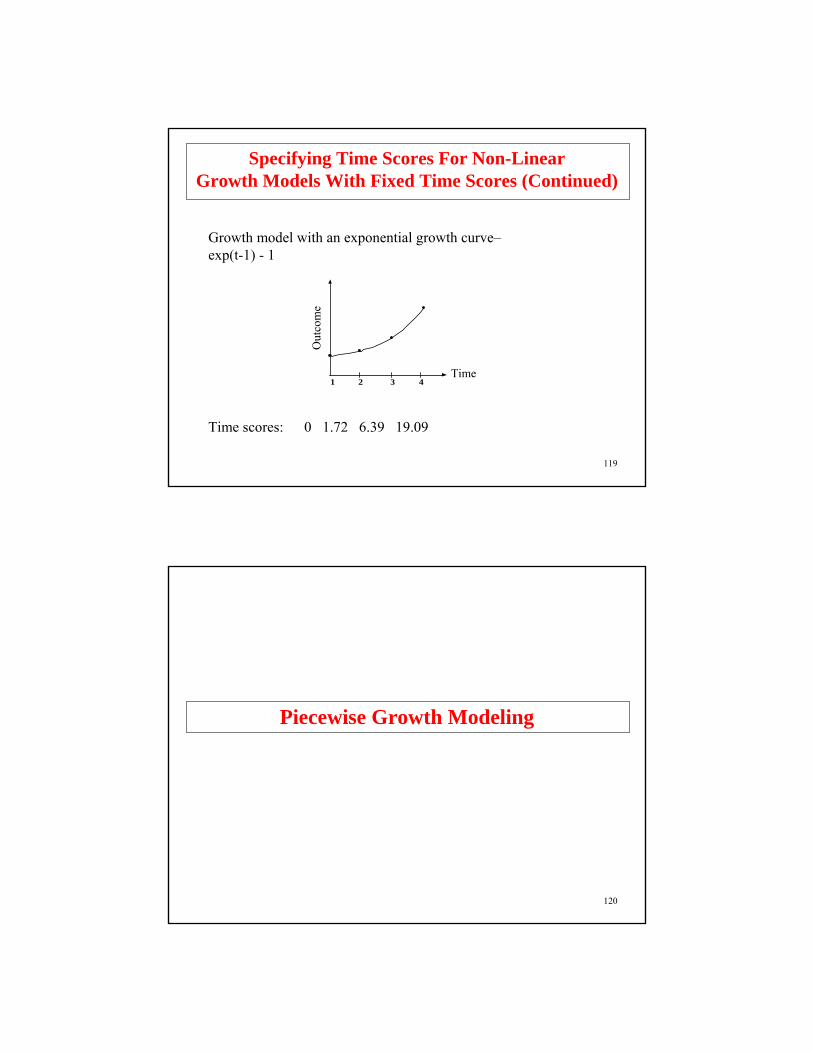
Specifying Time Scores For Non-LinearGrowth Models With Fixed Time Scores (Continued)
Growth model with an exponential growth curve–exp(t-1) - 1
Time scores: 0 1.72 6.39 19.09
1 2 3 4
Out
com
e
Time
120
Piecewise Growth Modeling

121
Piecewise Growth Modeling
• Can be used to represent different phases of development• Can be used to capture non-linear growth• Each piece has its own growth factor(s)• Each piece can have its own coefficients for covariates
20
15
10
5
01 2 3 4 5 6
One intercept growth factor, two slope growth factorss1: 0 1 2 2 2 2 Time scores piece 1s2: 0 0 0 1 2 3 Time scores piece 2
122
Piecewise Growth Modeling (Continued)
20
15
10
5
01 2 3 4 5 6
Two intercept growth factors, two slope growth factors0 1 2 Time scores piece 1
0 1 2 Time scores piece 2
Sequential model
123
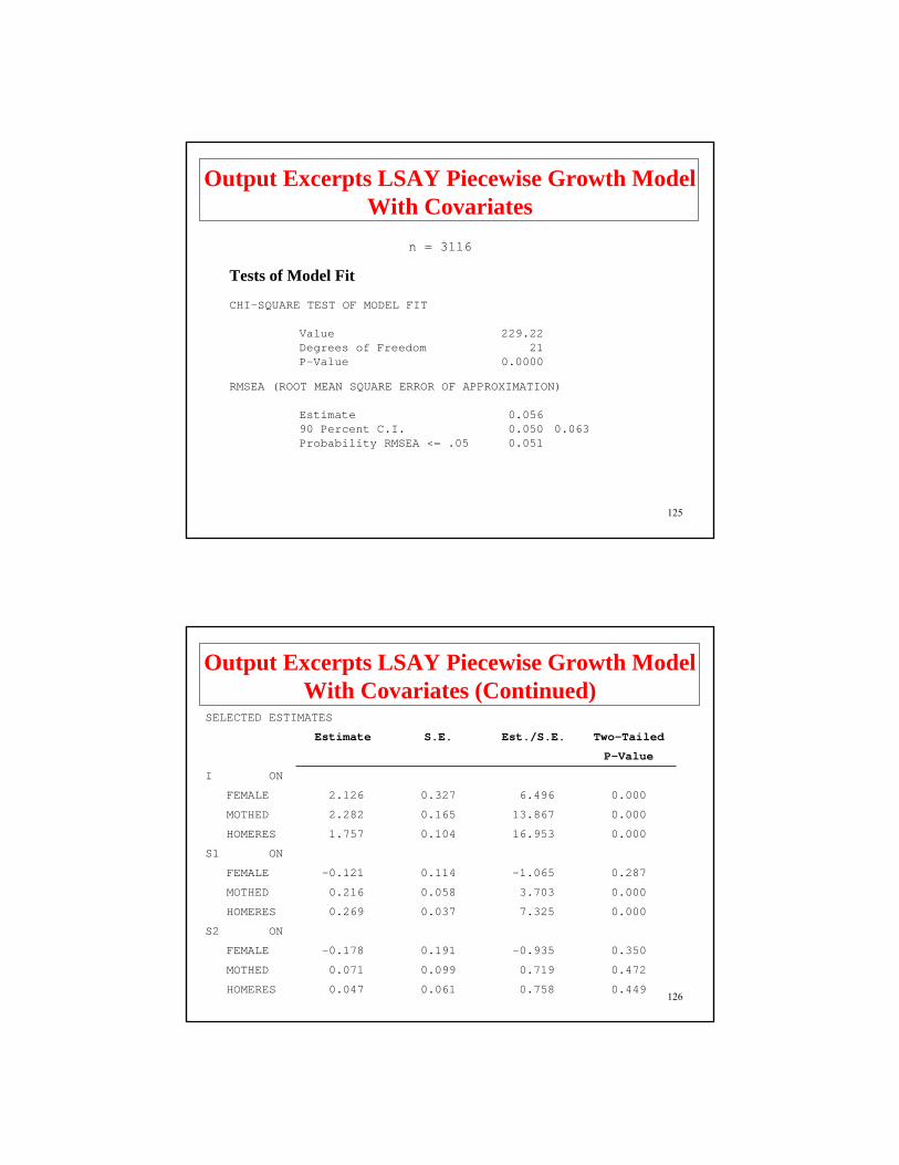
LSAY Piecewise Linear Growth Modeling: Grades 7-10 and 10-12
math7 math8 math9 math10
i s1 s2
321
math11 math12
3 3 21
124
Input For LSAY Piecewise Growth ModelWith Covariates
MODEL: i s1 | math7@0 math8@1 math9@2 math10@3 math11@3 math12@3;i s2 | math7@0 math8@0 math9@0 math10@0 math11@1 math12@2;i s1 s2 ON female mothed homeres;
Alternative language:
MODEL: i BY math7-math12@1;s1 BY math7@0 math8@1 math9@2 math10@3 math11@3 math12@3;s2 BY math7@0 math8@0 math9@0 math10@0 math11@1 math12@2;[math7-math12@0];[i s1 s2];i s1 s2 ON female mothed homeres;
125
n = 3116
Tests of Model Fit
CHI-SQUARE TEST OF MODEL FIT
Value 229.22 Degrees of Freedom 21P-Value 0.0000
RMSEA (ROOT MEAN SQUARE ERROR OF APPROXIMATION)
Estimate 0.05690 Percent C.I. 0.050 0.063Probability RMSEA <= .05 0.051
Output Excerpts LSAY Piecewise Growth Model With Covariates
126
Output Excerpts LSAY Piecewise Growth Model With Covariates (Continued)
SELECTED ESTIMATES
Estimate S.E. Est./S.E. Two-Tailed
P-Value
I ON
FEMALE 2.126 0.327 6.496 0.000
MOTHED 2.282 0.165 13.867 0.000
HOMERES 1.757 0.104 16.953 0.000
S1 ON
FEMALE -0.121 0.114 -1.065 0.287
MOTHED 0.216 0.058 3.703 0.000
HOMERES 0.269 0.037 7.325 0.000
S2 ON
FEMALE -0.178 0.191 -0.935 0.350
MOTHED 0.071 0.099 0.719 0.472
HOMERES 0.047 0.061 0.758 0.449
127
Intermediate Growth Models
128
Growth Model With Individually-Varying TimesOf Observation And Random Slopes
For Time-Varying Covariates

129
Growth Modeling In Multilevel Terms
Time point t, individual i (two-level modeling, no clustering):
yti : repeated measures of the outcome, e.g. math achievementa1ti : time-related variable; e.g. grade 7-10a2ti : time-varying covariate, e.g. math course takingxi : time-invariant covariate, e.g. grade 7 expectations
Two-level analysis with individually-varying times of observation and random slopes for time-varying covariates:
Level 1: yti = π0i + π1i a1ti + π2ti a2ti + eti , (55)
π 0i = ß00 + ß01 xi + r0i ,π 1i = ß10 + ß11 xi + r1i , (56)π 2i = ß20 + ß21 xi + r2i .
Level 2:
130
i
s
stvc
mothed
homeres
female
crs7
math7 math8 math9 math10
crs8 crs9 crs10

131
TITLE: Growth model with individually varying times of observation and random slopes
DATA: FILE IS lsaynew.dat; FORMAT IS 3F8.0 F8.4 8F8.2 3F8.0;
VARIABLE: NAMES ARE math7 math8 math9 math10 crs7 crs8 crs9
crs10 female mothed homeres a7-a10;
! crs7-crs10 = highest math course taken during each! grade (0=no course, 1=low, basic, 2=average, 3=high.
! 4=pre-algebra, 5=algebra I, 6=geometry,
! 7=algebra II, 8=pre-calc, 9=calculus)
MISSING ARE ALL (9999);
CENTER = GRANDMEAN (crs7-crs10 mothed homeres);TSCORES = a7-a10;
Input For Growth Model With Individually Varying Times Of Observation
132
DEFINE: math7 = math7/10;math8 = math8/10;math9 = math9/10;math10 = math10/10;
ANALYSIS: TYPE = RANDOM MISSING;ESTIMATOR = ML;MCONVERGENCE = .001;
MODEL: i s | math7-math10 AT a7-a10;stvc | math7 ON crs7;stvc | math8 ON crs8;stvc | math9 ON crs9;stvc | math10 ON crs10;i ON female mothed homeres;s ON female mothed homeres;stvc ON female mothed homeres;i WITH s;stvc WITH i;stvc WITH s;
OUTPUT: TECH8;
Input For Growth Model With Individually Varying Times Of Observation (Continued)
133
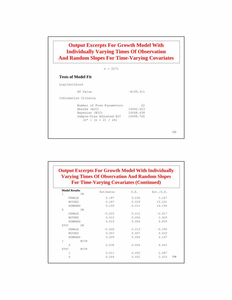
Output Excerpts For Growth Model WithIndividually Varying Times Of Observation
And Random Slopes For Time-Varying Covariates
n = 2271
Tests of Model Fit
Loglikelihood
H0 Value -8199.311
Information Criteria
Number of Free Parameters 22Akaike (AIC) 16442.623Bayesian (BIC) 16568.638Sample-Size Adjusted BIC 16498.740
(n* = (n + 2) / 24)
134
I ONFEMALE 0.187 0.036 5.247MOTHED 0.187 0.018 10.231HOMERES 0.159 0.011 14.194
S ONFEMALE -0.025 0.012 -2.017MOTHED 0.015 0.006 2.429HOMERES 0.019 0.004 4.835
STVC ONFEMALE -0.008 0.013 -0.590MOTHED 0.003 0.007 0.429HOMERES 0.009 0.004 2.167
I WITHS 0.038 0.006 6.445
STVC WITHI 0.011 0.005 2.087S 0.004 0.002 2.033
Output Excerpts For Growth Model With Individually Varying Times Of Observation And Random Slopes
For Time-Varying Covariates (Continued)Model Results Estimates S.E. Est./S.E.
135
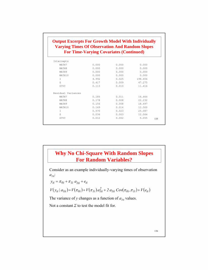
InterceptsMATH7 0.000 0.000 0.000MATH8 0.000 0.000 0.000MATH9 0.000 0.000 0.000MATH10 0.000 0.000 0.000I 4.992 0.025 198.456S 0.417 0.009 47.275STVC 0.113 0.010 11.416
Residual VariancesMATH7 0.185 0.011 16.464MATH8 0.178 0.008 22.232MATH9 0.156 0.008 18.497MATH10 0.169 0.014 12.500I 0.570 0.023 25.087S 0.036 0.003 12.064STVC 0.012 0.002 5.055
Output Excerpts For Growth Model With Individually Varying Times Of Observation And Random Slopes
For Time-Varying Covariates (Continued)
136
Why No Chi-Square With Random Slopes For Random Variables?
The variance of y changes as a function of a1ti values.
Not a constant Σ to test the model fit for.
Consider as an example individually-varying times of observation a1ti:
( ) ( ) ( ) ( ) ( )tii1i0ti12ti1i1i0ti1ti eV ,Cov a 2a V V a|yV +++= ππππ
titi1i1i0ti ea y ++= ππ
137
Maximum-Likelihood Alternatives
Note that [y, x] = [y | x] * [x], where the marginal distribution [x] is unrestricted.
Normal theory ML for• [y, x]: Gives the same results as [y | x] when there is no
missing data (Joreskog & Goldberger, 1975). Typically used in SEM– With missing data on x, the normality assumption for x is
an additional assumption not used with [y | x]• [y | x]: Makes normality assumptions for residuals, not for
x. Typically used outside SEM– Used with Type = Random, Type = Mixture, and with
categorical, censored, and count outcomes– Deletes individuals with missing on any x
• [y, x] versus [y | x] gives different sample sizes and the likelihood and BIC values are not on a comparable scale
138
Alternative Models With Time-Varying Covariates

139
Alternative ModelsWith Time-Varying Covariates
i
s
stvc
mothed
homeres
female
crs7
math7 math8 math9 math10
crs8 crs9 crs10
i
s
mothed
homeres
female
crs7
math7 math8 math9 math10
crs8 crs9 crs10
Model M1 Model M2
140
Input Excerpts Model M1
ANALYSIS: TYPE = RANDOM; ! gives loglikelihood in [y | x] metric
MODEL: i s | math7@0 math8@1 math9@2 math10@3;
i s ON female mothed homeres;
math7 ON mthcrs7;math8 ON mthcrs8;
math9 ON mthcrs9;
math10 ON mthcrs10;
141
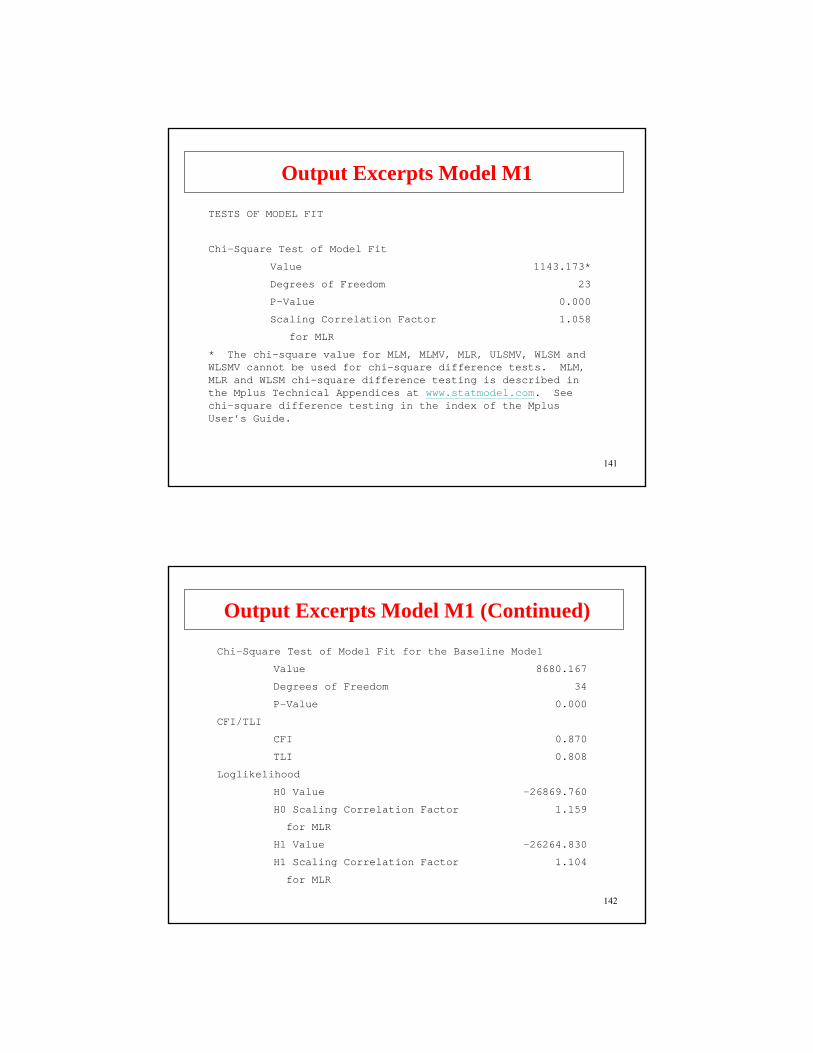
Output Excerpts Model M1
TESTS OF MODEL FIT
Chi-Square Test of Model Fit
Value 1143.173*
Degrees of Freedom 23
P-Value 0.000
Scaling Correlation Factor 1.058
for MLR
* The chi-square value for MLM, MLMV, MLR, ULSMV, WLSM and WLSMV cannot be used for chi-square difference tests. MLM, MLR and WLSM chi-square difference testing is described in the Mplus Technical Appendices at www.statmodel.com. See chi-square difference testing in the index of the Mplus User’s Guide.
142
Output Excerpts Model M1 (Continued)
Chi-Square Test of Model Fit for the Baseline Model
Value 8680.167
Degrees of Freedom 34
P-Value 0.000
CFI/TLI
CFI 0.870
TLI 0.808
Loglikelihood
H0 Value -26869.760
H0 Scaling Correlation Factor 1.159
for MLR
H1 Value -26264.830
H1 Scaling Correlation Factor 1.104
for MLR
143
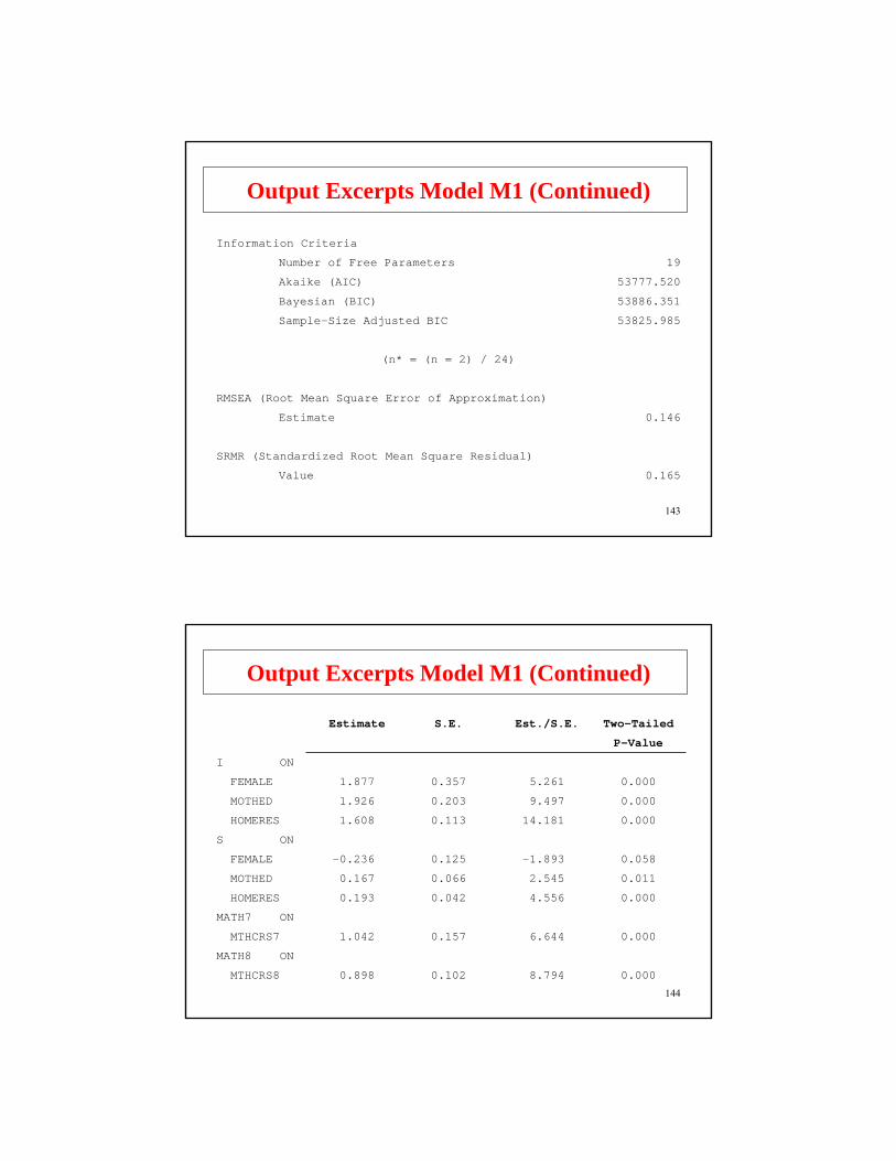
Output Excerpts Model M1 (Continued)
Information Criteria
Number of Free Parameters 19
Akaike (AIC) 53777.520
Bayesian (BIC) 53886.351
Sample-Size Adjusted BIC 53825.985
(n* = (n = 2) / 24)
RMSEA (Root Mean Square Error of Approximation)
Estimate 0.146
SRMR (Standardized Root Mean Square Residual)
Value 0.165
144
Output Excerpts Model M1 (Continued)
Estimate S.E. Est./S.E. Two-Tailed
P-Value
I ON
FEMALE 1.877 0.357 5.261 0.000
MOTHED 1.926 0.203 9.497 0.000
HOMERES 1.608 0.113 14.181 0.000
S ON
FEMALE -0.236 0.125 -1.893 0.058
MOTHED 0.167 0.066 2.545 0.011
HOMERES 0.193 0.042 4.556 0.000
MATH7 ON
MTHCRS7 1.042 0.157 6.644 0.000
MATH8 ON
MTHCRS8 0.898 0.102 8.794 0.000

145
Output Excerpts Model M1 (Continued)Estimate S.E. Est./S.E. Two-Tailed
P-Value
MATH9 ON
MTHCRS9 0.929 0.087 10.638 0.000
MATH10 ON
MTHCRS10 0.911 0.102 8.966 0.000
S WITH
I 4.200 0.687 6.113 0.000
Intercepts
MATH7 0.000 0.000 999.000 999.000
MATH8 0.000 0.000 999.000 999.000
MATH9 0.000 0.000 999.000 999.000
MATH10 0.000 0.000 999.000 999.000
I 50.063 0.263 190.158 0.000
S 4.202 0.096 43.621 0.000
146
Output Excerpts Model M1 (Continued)
Estimate S.E. Est./S.E. Two-Tailed
P-Value
Residual Variances
MATH7 18.640 1.341 13.895 0.000
MATH8 18.554 1.002 18.518 0.000
MATH9 16.672 1.010 16.501 0.000
MATH10 17.795 1.671 10.651 0.000
I 58.919 2.393 24.622 0.000
S 3.800 0.359 10.581 0.000
147
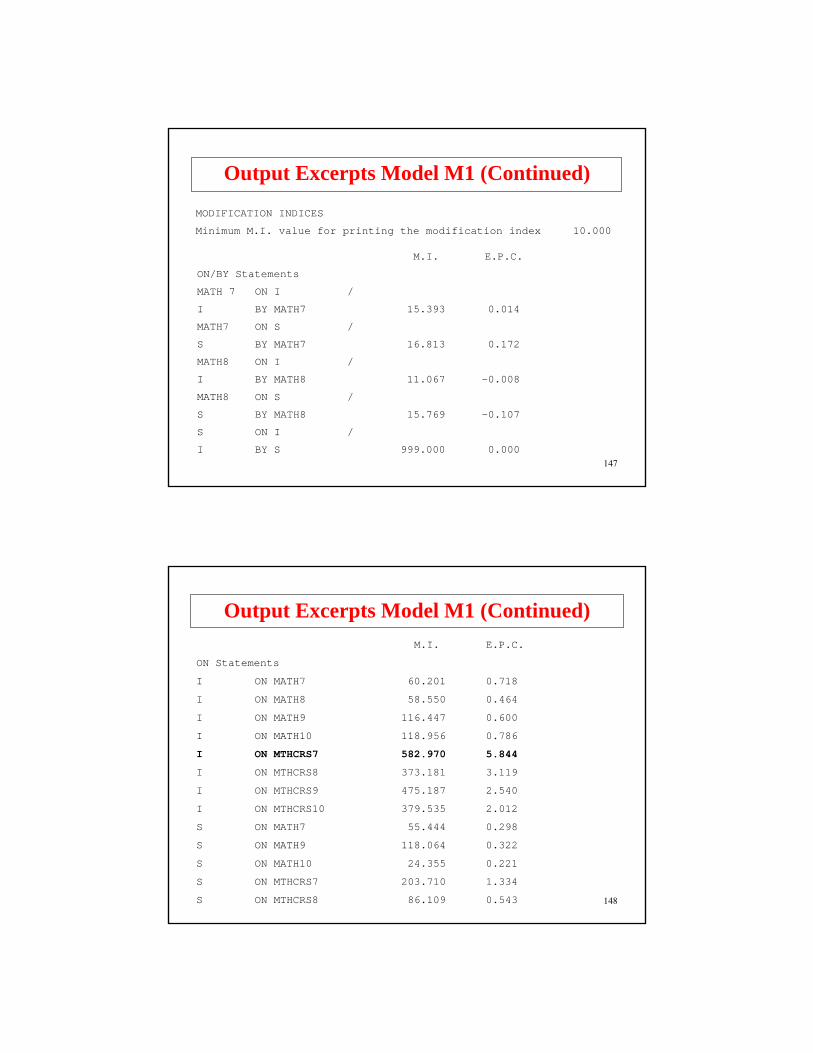
Output Excerpts Model M1 (Continued)
MODIFICATION INDICES
Minimum M.I. value for printing the modification index 10.000
M.I. E.P.C.
ON/BY Statements
MATH 7 ON I /
I BY MATH7 15.393 0.014
MATH7 ON S /
S BY MATH7 16.813 0.172
MATH8 ON I /
I BY MATH8 11.067 -0.008
MATH8 ON S /
S BY MATH8 15.769 -0.107
S ON I /
I BY S 999.000 0.000
148
Output Excerpts Model M1 (Continued)M.I. E.P.C.
ON Statements
I ON MATH7 60.201 0.718
I ON MATH8 58.550 0.464
I ON MATH9 116.447 0.600
I ON MATH10 118.956 0.786
I ON MTHCRS7 582.970 5.844
I ON MTHCRS8 373.181 3.119
I ON MTHCRS9 475.187 2.540
I ON MTHCRS10 379.535 2.012
S ON MATH7 55.444 0.298
S ON MATH9 118.064 0.322
S ON MATH10 24.355 0.221
S ON MTHCRS7 203.710 1.334
S ON MTHCRS8 86.109 0.543

149
Output Excerpts Model M1 (Continued)M.I. E.P.C.
S ON MTHCRS9 90.560 0.453
S ON MTHCRS10 118.478 0.559
MATH7 ON MATH7 15.393 0.014
MATH7 ON MATH8 17.359 0.013
MATH7 ON MATH9 14.805 0.011
MATH7 ON MATH10 18.991 0.012
MATH7 ON MTHCRS8 48.865 0.873
MATH7 ON MTHCRS9 63.490 0.676
MATH7 ON MTHCRS10 22.160 0.337
MATH8 ON MATH8 11.438 -0.007
MATH8 ON MATH10 13.204 -0.007
MATH8 ON MTHCRS7 82.739 1.467
MATH8 ON MTHCRS9 12.743 0.321
150
Output Excerpts Model M1 (Continued)M.I. E.P.C.
MATH9 ON MTHCRS7 26.183 0.776
MATH9 ON MTHCRS8 16.027 0.494
MATH9 ON MTHCRS10 69.480 0.781
MATH10 ON MTHCRS8 19.665 0.629
MATH10 ON MTHCRS9 48.678 0.911

151
Alternative Models With Time-Varying Covariates
Model Loglikelihood # of parameters BIC
M1 -26,870 19 53,886
M2 -26,846 22 53,861
M3 -26,463 26 53,127
n = 2271 (using [y|x] approach)
M1: Fixed slopes for TVCs, varying across grade
M2: Random slope for TVCs, same across grade
M3: M2 + i and s regressed on TVCs (see model diagram)
152
i
s
stvc
mothed
homeres
female
crs7
math7 math8 math9 math10
crs8 crs9 crs10
Time-Varying Covariates: Model M3
153
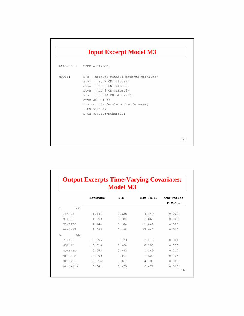
Input Excerpt Model M3
ANALYSIS: TYPE = RANDOM;
MODEL: i s | math7@0 math8@1 math9@2 math10@3;
stvc | math7 ON mthcrs7;
stvc | math8 ON mthcrs8;stvc | math9 ON mthcrs9;
stvc | math10 ON mthcrs10;
stvc WITH i s;i s stvc ON female mothed homeres;
i ON mthcrs7;
s ON mthcrs8-mthcrs10;
154
Output Excerpts Time-Varying Covariates: Model M3
Estimate S.E. Est./S.E. Two-Tailed
P-Value
I ON
FEMALE 1.444 0.325 4.449 0.000
MOTHED 1.259 0.184 6.860 0.000
HOMERES 1.144 0.104 11.041 0.000
MTHCRS7 5.095 0.188 27.040 0.000
S ON
FEMALE -0.395 0.123 -3.215 0.001
MOTHED -0.018 0.064 -0.283 0.777
HOMERES 0.052 0.042 1.249 0.212
MTHCRS8 0.099 0.061 1.627 0.104
MTHCRS9 0.254 0.061 4.188 0.000
MTHCRS10 0.341 0.053 6.471 0.000

155
Estimate S.E. Est./S.E. Two-Tailed
P-Value
STVC ON
FEMALE -0.083 0.123 -0.677 0.499
MOTHED 0.009 0.066 0.129 0.898
HOMERES 0.070 0.041 1.710 0.087
STVC WITH
I -0.078 0.453 -0.173 0.863
S 0.015 0.185 0.083 0.934
S WITH
I 0.480 0.630 0.762 0.446
Intercepts
MATH7 0.000 0.000 999.000 999.000
MATH8 0.000 0.000 999.000 999.000
Output Excerpts: Model M3 (Continued)
156
Estimate S.E. Est./S.E. Two-Tailed
P-Value
MATH9 0.000 0.000 999.000 999.000
MATH10 0.000 0.000 999.000 999.000
I 50.244 0.240 209.085 0.000
S 4.257 0.094 45.071 0.000
STVC 0.231 0.106 2.188 0.029
Residual Variances
MATH7 18.968 1.304 14.541 0.000
MATH8 17.061 0.931 18.322 0.000
MATH9 15.624 0.936 16.690 0.000
MATH10 16.550 1.494 11.074 0.000
I 44.980 1.891 23.792 0.000
S 3.423 0.338 10.118 0.000
STVC 0.615 0.255 2.410 0.016
Output Excerpts: Model M3 (Continued)
157
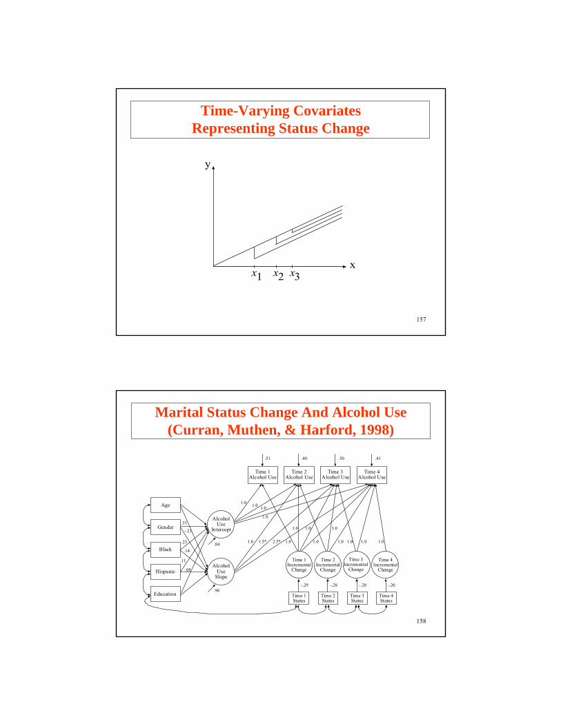
Time-Varying Covariates Representing Status Change
x
y
x1 x2 x3
158
Marital Status Change And Alcohol Use(Curran, Muthen, & Harford, 1998)
AlcoholUse
Intercept
AlcoholUse
Slope
Time 1Alcohol Use
Time 2Alcohol Use
Time 3Alcohol Use
Time 4Alcohol Use
Time 1Incremental
Change
Time 2Incremental
Change
Time 3Incremental
Change
Time 4Incremental
Change
Time 1Status
Time 2Status
Time 3Status
Time 4Status
Age
Gender
Black
Hispanic
Education
.84
.96-.29 -.28 -.20 -.20
.51 .48 .50 .41
1.0 1.0 1.0
1.0
1.0 1.5* 2.5* 1.0
1.0 1.0
1.0
1.0
1.0 1.0 1.0 1.0
.31
-.21
.23
.14
.11
.08
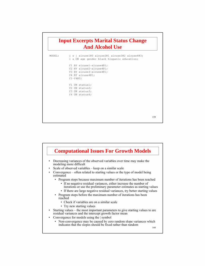
Input Excerpts Marital Status Change And Alcohol Use
MODEL: i s | alcuse1@0 alcuse2@1 alcuse3@2 alcuse4@3;i s ON age gender black hispanic education;
f1 BY alcuse1-alcuse4@1;f2 BY alcuse2-alcuse4@1;f3 BY alcuse3-alcuse4@1;f4 BY alcuse4@1;f1-f4@0;
f1 ON status1;f2 ON status2;f3 ON status3;f4 ON status4;
159
160
• Decreasing variances of the observed variables over time may make the modeling more difficult
• Scale of observed variables – keep on a similar scale• Convergence – often related to starting values or the type of model being
estimated• Program stops because maximum number of iterations has been reached
• If no negative residual variances, either increase the number ofiterations or use the preliminary parameter estimates as starting values
• If there are large negative residual variances, try better starting values• Program stops before the maximum number of iterations has been
reached• Check if variables are on a similar scale• Try new starting values
• Starting values – the most important parameters to give starting values to are residual variances and the intercept growth factor mean
• Convergence for models using the | symbol• Non-convergence may be caused by zero random slope variances which
indicates that the slopes should be fixed rather than random
Computational Issues For Growth Models

161
Advantages Of Growth Modeling In A Latent Variable Framework
• Flexible curve shape• Individually-varying times of observation• Regressions among random effects• Multiple processes• Modeling of zeroes• Multiple populations• Multiple indicators• Embedded growth models• Categorical latent variables: growth mixtures
162
Regressions Among Random Effects

163
Regressions Among Random EffectsStandard multilevel model (where xt = 0, 1, …, T):
Level 1: yti = η0i + η1i xt + εti , (1)Level 2a: η0i = α0 + γ0 wi + ζ0i , (2)Level 2b: η1i = α1 + γ1 wi + ζ1i . (3)
A useful type of model extension is to replace (3) by the regression equationη1i = α + β η0i + γ wi + ζi . (4)
Example: Blood Pressure (Bloomqvist, 1977)
η0 η1
w
η0 η1
w
164
i
mthcrs7
s
math7 math8 math9 math10
Growth Model With An Interaction
b1
b2
b3

165
TITLE: growth model with an interaction between a latent and an observed variable
DATA: FILE IS lsay.dat;VARIABLE: NAMES ARE math7 math8 math9 math10 mthcrs7;
MISSING ARE ALL (9999);CENTERING = GRANDMEAN (mthcrs7);
DEFINE: math7 = math7/10;math8 = math8/10;math9 = math9/10;math10 = math10/10;
ANALYSIS: TYPE=RANDOM MISSING;MODEL: i s | math7@0 math8@1 math9@2 math10@3;
[math7-math10] (1); !growth language defaults[i@0 s]; !overridden
inter | i XWITH mthcrs7;s ON i mthcrs7 inter;i ON mthcrs7;
OUTPUT: SAMPSTAT STANDARDIZED TECH1 TECH8;
Input For A Growth Model With An InteractionBetween A Latent And An Observed Variable
166
Tests Of Model FitLoglikelihood
H0 Value -10068.944Information Criteria
Number of Free Parameters 12Akaike (AIC) 20161.887Bayesian (BIC) 20234.365Sample-Size Adjusted BIC
(n* = (n + 2) / 24)20196.236
Output Excerpts Growth Model With An InteractionBetween A Latent And An Observed Variable
167
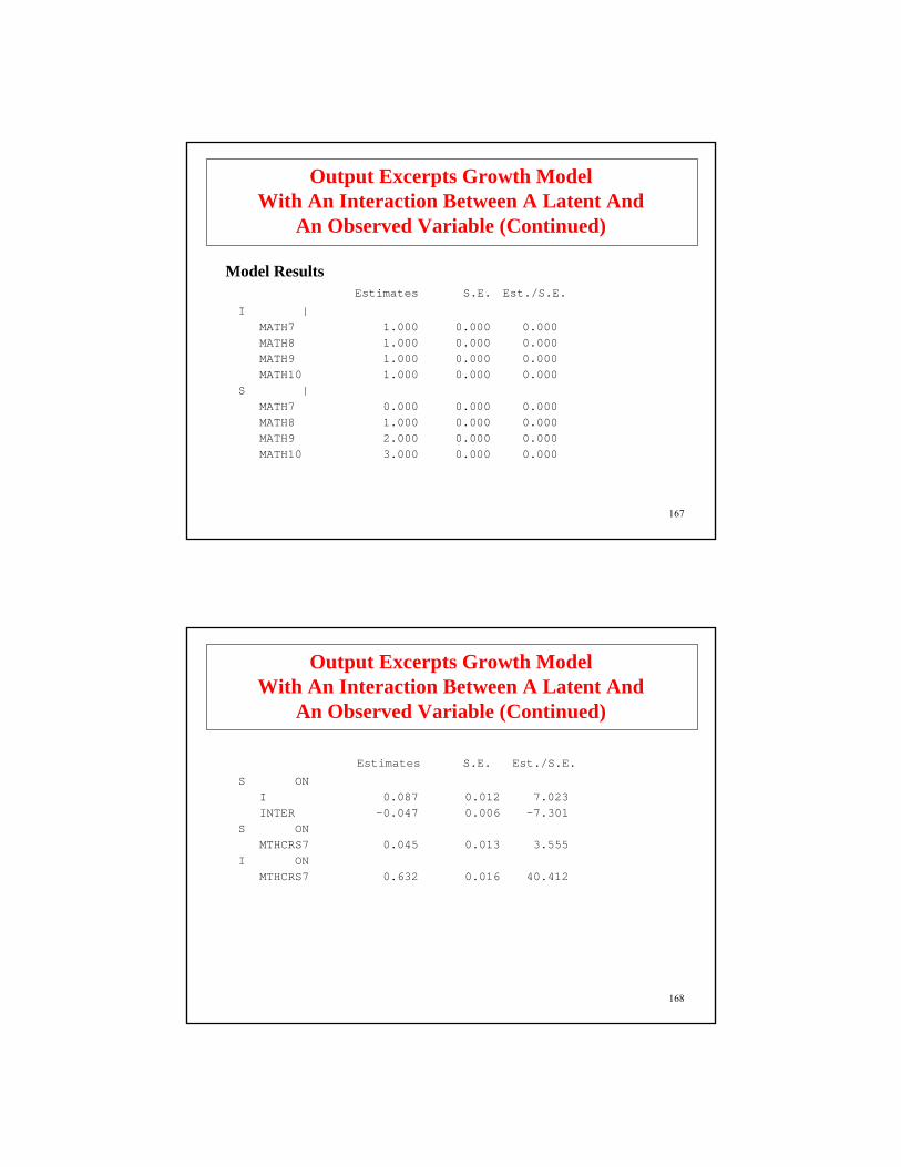
Model Results
I |MATH7 1.000 0.000 0.000MATH8 1.000 0.000 0.000MATH9 1.000 0.000 0.000MATH10 1.000 0.000 0.000
S |MATH7 0.000 0.000 0.000MATH8 1.000 0.000 0.000MATH9 2.000 0.000 0.000MATH10 3.000 0.000 0.000
Estimates S.E. Est./S.E.
Output Excerpts Growth Model With An Interaction Between A Latent And
An Observed Variable (Continued)
168
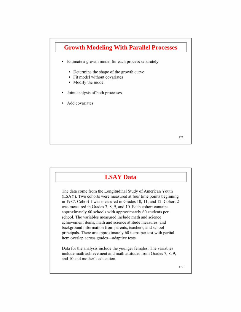
Output Excerpts Growth Model With An Interaction Between A Latent And
An Observed Variable (Continued)
S ONI 0.087 0.012 7.023INTER -0.047 0.006 -7.301
S ONMTHCRS7 0.045 0.013 3.555
I ONMTHCRS7 0.632 0.016 40.412
Estimates S.E. Est./S.E.

169
InterceptsMATH7 5.019 0.015 341.587MATH8 5.019 0.015 341.587MATH9 5.019 0.015 341.587MATH10 5.019 0.015 341.587I 0.000 0.000 0.000S 0.417 0.007 57.749
Residual VariancesMATH7 0.184 0.011 16.117MATH8 0.178 0.009 20.109MATH9 0.164 0.009 18.369MATH10 0.173 0.015 11.509I 0.528 0.018 28.935S 0.037 0.004 10.027
Output Excerpts Growth Model With An Interaction Between A Latent And
An Observed Variable (Continued)
Estimates S.E. Est./S.E.
170
• Model equation for slope ss = a + b1*i + b2*mthcrs7 + b3*i*mthcrs7 + e
or, using a moderator function (Klein & Moosbrugger, 2000) wherei moderates the influence of mthcrs7 on ss = a + b1*i + (b2 + b3*i)*mthcrs7 + e
• Estimated model
Unstandardizeds = 0.417 + 0.087*i + (0.045 – 0.047*i)*mthcrs7
Standardized with respect to i and mthcrs7s = 0.42 + 0.08 * i + (0.04-0.04*i)*mthcrs7
Interpreting The Effect Of The Interaction BetweenInitial Status Of Growth In Math Achievement
And Course Taking In Grade 6

171
• Interpretation of the standardized solutionAt the mean of i, which is zero, the slope increases 0.04 for 1 SD increase in mthcrs7
At 1 SD below the mean of i, which is zero, the slope increases 0.08 for 1 SD increase in mthcrs7
At 1 SD above the mean of i, which is zero, the slope does not increase as a function of mthcrs7
Interpreting The Effect Of The Interaction BetweenInitial Status Of Growth In Math Achievement
And Course Taking In Grade 6 (Continued)
172
Growth Modeling With Parallel Processes

173
Advantages Of Growth Modeling In A Latent Variable Framework
• Flexible curve shape• Individually-varying times of observation• Regressions among random effects• Multiple processes• Modeling of zeroes• Multiple populations• Multiple indicators• Embedded growth models• Categorical latent variables: growth mixtures
174
Multiple Processes
• Parallel processes
• Sequential processes
175
• Estimate a growth model for each process separately
• Determine the shape of the growth curve• Fit model without covariates• Modify the model
• Joint analysis of both processes
• Add covariates
Growth Modeling With Parallel Processes
176
The data come from the Longitudinal Study of American Youth(LSAY). Two cohorts were measured at four time points beginningin 1987. Cohort 1 was measured in Grades 10, 11, and 12. Cohort 2was measured in Grades 7, 8, 9, and 10. Each cohort containsapproximately 60 schools with approximately 60 students perschool. The variables measured include math and scienceachievement items, math and science attitude measures, andbackground information from parents, teachers, and schoolprincipals. There are approximately 60 items per test with partialitem overlap across grades—adaptive tests.
Data for the analysis include the younger females. The variablesinclude math achievement and math attitudes from Grades 7, 8, 9,and 10 and mother’s education.
LSAY Data
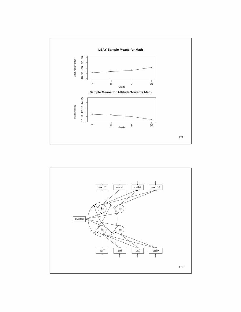
177
Grade
Mat
h A
chie
vem
ent
7 8 9 10
4050
6070
8011
1213
1415
7 8 9 10
Mat
h A
ttitu
de
Grade
LSAY Sample Means for Math
Sample Means for Attitude Towards Math
10
178
math7 math8 math9
im sm
mothed
ia sa
att7 att8 att9 att10
math10

179
Correlations Between Processes
• Through covariates
• Through growth factors (growth factor residuals)
• Through outcome residuals
180
TITLE: LSAY For Younger Females With Listwise Deletion Parallel Process Growth Model-Math Achievement and Math Attitudes
DATA: FILE IS lsay.dat; FORMAT IS 3f8 f8.4 8f8.2 3f8 2f8.2;
VARIABLE: NAMES ARE cohort id school weight math7 math8 math9 math10 att7 att8 att9 att10 gender mothed homeres
ses3 sesq3;
USEOBS = (gender EQ 1 AND cohort EQ 2); MISSING = ALL (999);USEVAR = math7-math10 att7-att10 mothed;
Input For LSAY Parallel Process Growth Model

181
MODEL: im sm | math7@0 math8@1 math9 math10;ia sa | att7@0 att8@1 att9@2 att10@3;im-sa ON mothed;
Input For LSAY Parallel Process Growth Model(Continued)
OUTPUT: MODINDICES STANDARDIZED;
im BY math7-math10@1;sm BY math7@0 math8@1 math9 math10;
ia BY att7-att10@1;sa BY att7@0 att8@1 att9@2 att10@3;
[math7-math10@0 att7-att10@0];[im sm ia sa];
im-sa ON mothed;
Alternative language:
182
n = 910
Tests of Model Fit
Chi-Square Test of Model Fit
Value 43.161Degrees of Freedom 24P-Value .0095
RMSEA (Root Mean Square Error Of Approximation)
Estimate .03090 Percent C.I. .015 .044Probability RMSEA <= .05 .992
Output Excerpts LSAY ParallelProcess Growth Model

183
IM ONMOTHED 2.462 .280 8.798 .311 .303
SM ONMOTHED .145 .066 2.195 .132 .129
IA ONMOTHED .053 .086 .614 .025 .024
SA ONMOTHED .012 .035 .346 .017 .017
Output Excerpts LSAY ParallelProcess Growth Model (Continued)
Estimates S.E. Est./S.E. Std StdYX
184
SM WITHIM 3.032 .580 5.224 .350 .350
IA WITHIM 4.733 .702 6.738 .282 .282SM .544 .164 3.312 .235 .235
SA WITHIM -.276 .279 -.987 -.049 -.049SM .130 .066 1.976 .168 .168IA -.567 .115 -4.913 -.378 -.378
Output Excerpts LSAY ParallelProcess Growth Model (Continued)
Estimates S.E. Est./S.E. Std StdYX

185
Categorical Outcomes:Logistic And Probit Regression
186
Probability varies as a function of x variables (here x1, x2)
P(u = 1 | x1, x2) = F[β0 + β1 x1 + β2 x2 ], (22)
P(u = 0 | x1 , x2) = 1 - P[u = 1 | x1 , x2], where F[z] is either the standard normal (Φ[z]) or logistic (1/[1 + e-z]) distributionfunction.
Example: Lung cancer and smoking among coal minersu lung cancer (u = 1) or not (u = 0)x1 smoker (x1 = 1), non-smoker (x1 = 0)x2 years spent in coal mine
Categorical Outcomes: Logit And Probit Regression

187
P(u = 1 | x1, x2) = F [β0 + β1 x1 + β2 x2 ], (22)
x2
Probit / Logitx1 = 1
x1 = 0
Categorical Outcomes: Logit And Probit Regression
P( u = 1 x1 , x2)
0
1
x2
0.5
x1 = 0
x1 = 1
188
Interpreting Logit And Probit Coefficients
• Sign and significance
• Odds and odds ratios
• Probabilities
189
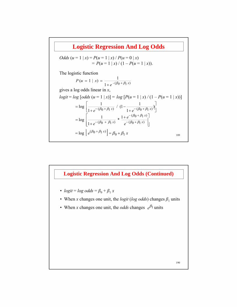
Logistic Regression And Log Odds
Odds (u = 1 | x) = P(u = 1 | x) / P(u = 0 | x)= P(u = 1 | x) / (1 – P(u = 1 | x)).
The logistic function
gives a log odds linear in x,
⎥⎦⎤
⎢⎣⎡
+−
+= +−+− )
111(/
11log )10()10( x x e
e
ββββ
[ ] x e x 10
)10(log ββββ +== +
⎥⎥⎦
⎤
⎢⎢⎣
⎡ +
+= +−
+−
+− )10(
)10(
)10(1*
11log x
x
x ee
e ββ
ββ
ββ
logit = log [odds (u = 1 | x)] = log [P(u = 1 | x) / (1 – P(u = 1 | x))]
)1(11)|1( x 0 - e
x u P ββ ++==
190
Logistic Regression And Log Odds (Continued)
• logit = log odds = β0 + β1 x
• When x changes one unit, the logit (log odds) changes β1 units
• When x changes one unit, the odds changes units1βe

191
Further Readings On Categorical Variable Analysis
Agresti, A. (2002). Categorical data analysis. Second edition. New York: John Wiley & Sons.
Agresti, A. (1996). An introduction to categorical data analysis. New York: Wiley.
Hosmer, D. W. & Lemeshow, S. (2000). Applied logistic regression. Second edition. New York: John Wiley & Sons.
Long, S. (1997). Regression models for categorical and limited dependent variables. Thousand Oaks: Sage.
192
Growth Models WithCategorical Outcomes
193
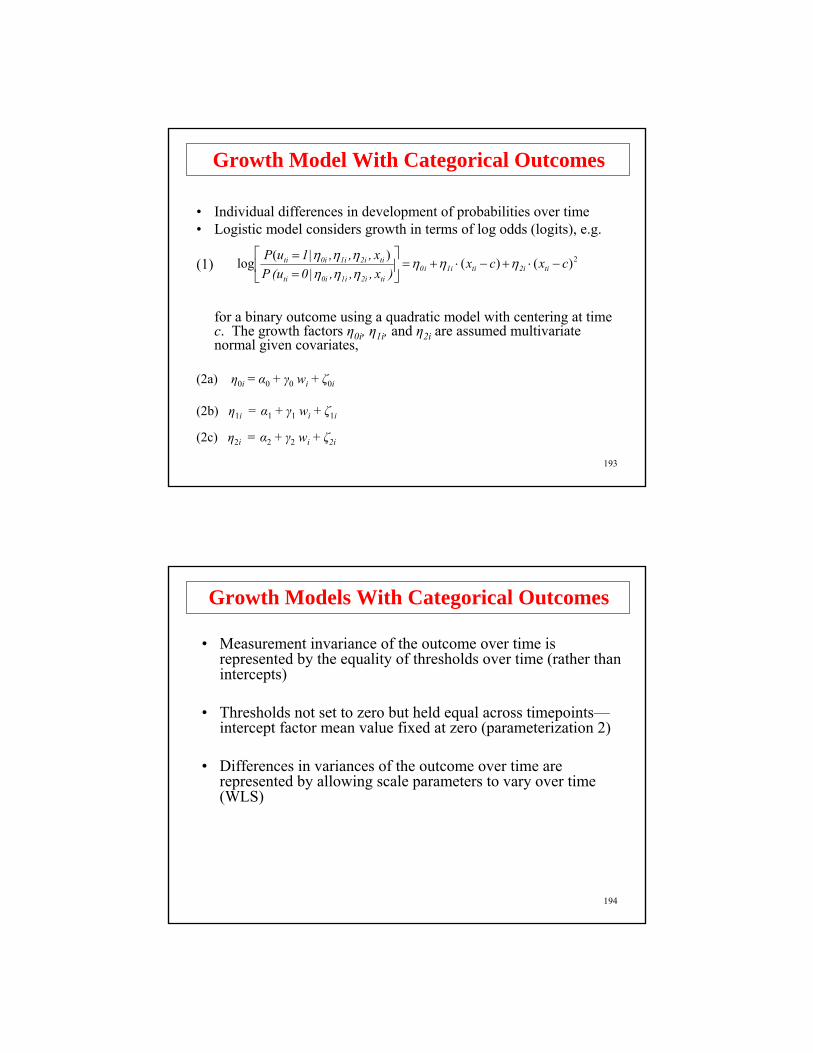
Growth Model With Categorical Outcomes
• Individual differences in development of probabilities over time• Logistic model considers growth in terms of log odds (logits), e.g.
(1)
for a binary outcome using a quadratic model with centering at time c. The growth factors η0i, η1i, and η2i are assumed multivariate normal given covariates,
(2a) η0i = α0 + γ0 wi + ζ0i
(2b) η1i = α1 + γ1 wi + ζ1i
(2c) η2i = α2 + γ2 wi + ζ2i
2)()()(log cxcx)x , , , | 0 (u P
x , , , | 1 uPti2itii1i0
ti2i1i0iti
ti2ii10iti −⋅+−⋅+=⎥⎦
⎤⎢⎣
⎡== ηηη
ηηηηηη
194
Growth Models With Categorical Outcomes
• Measurement invariance of the outcome over time is represented by the equality of thresholds over time (rather thanintercepts)
• Thresholds not set to zero but held equal across timepoints—intercept factor mean value fixed at zero (parameterization 2)
• Differences in variances of the outcome over time are represented by allowing scale parameters to vary over time (WLS)
195
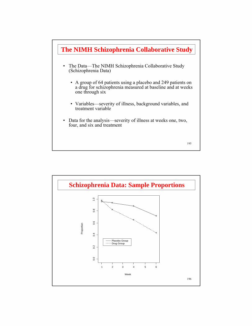
The NIMH Schizophrenia Collaborative Study
• The Data—The NIMH Schizophrenia Collaborative Study (Schizophrenia Data)
• A group of 64 patients using a placebo and 249 patients on a drug for schizophrenia measured at baseline and at weeks one through six
• Variables—severity of illness, background variables, and treatment variable
• Data for the analysis—severity of illness at weeks one, two, four, and six and treatment
196
Placebo GroupDrug Group
Pro
porti
on
Week
1 2 3 4 5 6
0.0
0.2
0.4
0.6
0.8
1.0
Schizophrenia Data: Sample Proportions
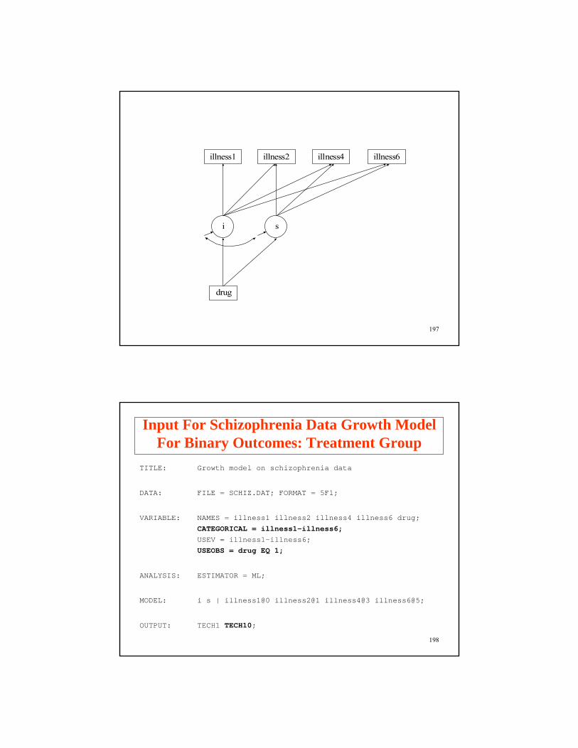
197
illness1 illness2 illness4 illness6
drug
i s
198
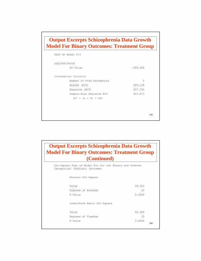
Input For Schizophrenia Data Growth ModelFor Binary Outcomes: Treatment Group
TITLE: Growth model on schizophrenia data
DATA: FILE = SCHIZ.DAT; FORMAT = 5F1;
VARIABLE: NAMES = illness1 illness2 illness4 illness6 drug;
CATEGORICAL = illness1-illness6;USEV = illness1-illness6;USEOBS = drug EQ 1;
ANALYSIS: ESTIMATOR = ML;
MODEL: i s | illness1@0 illness2@1 illness4@3 illness6@5;
OUTPUT: TECH1 TECH10;
199
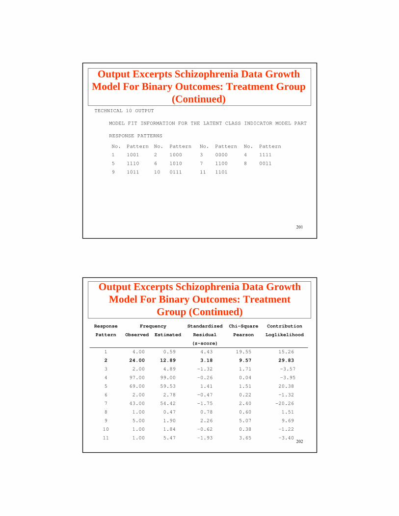
Output Excerpts Schizophrenia Data Growth Model For Binary Outcomes: Treatment Group
TEST OF MODEL FIT
Loglikelihood
H0 Value -405.068
Information Criteria
Number of Free Parameters 5
Akaike (AIC) 820.136
Bayesian (BIC) 837.724
Sample-Size Adjusted BIC 821.873
(n* = (n + 2) / 24)
200
Output Excerpts Schizophrenia Data Growth Model For Binary Outcomes: Treatment Group
(Continued)Chi-Square Test of Model Fit for the Binary and Ordered Categorical (Ordinal) Outcomes
Pearson Chi-Square
Value 49.923
Degrees of Freedom 10
P-Value 0.0000
Likelihood Ratio Chi-Square
Value 42.960
Degrees of Freedom 10
P-Value 0.0000
201
No. Pattern No. Pattern No. Pattern No. Pattern
1 1001 2 1000 3 0000 4 1111
5 1110 6 1010 7 1100 8 0011
9 1011 10 0111 11 1101
Output Excerpts Schizophrenia Data Growth Model For Binary Outcomes: Treatment Group
(Continued)TECHNICAL 10 OUTPUT
MODEL FIT INFORMATION FOR THE LATENT CLASS INDICATOR MODEL PART
RESPONSE PATTERNS
202
Output Excerpts Schizophrenia Data Growth Model For Binary Outcomes: Treatment
Group (Continued)Response Frequency Standardized Chi-Square Contribution
Pattern Observed Estimated Residual Pearson Loglikelihood
(z-score)
1 4.00 0.59 4.43 19.55 15.26
2 24.00 12.89 3.18 9.57 29.83
3 2.00 4.89 -1.32 1.71 -3.57
4 97.00 99.00 -0.26 0.04 -3.95
5 69.00 59.53 1.41 1.51 20.38
6 2.00 2.78 -0.47 0.22 -1.32
7 43.00 54.42 -1.75 2.40 -20.26
8 1.00 0.47 0.78 0.60 1.51
9 5.00 1.90 2.26 5.07 9.69
10 1.00 1.84 -0.62 0.38 -1.22
11 1.00 5.47 -1.93 3.65 -3.40

203
Output Excerpts Schizophrenia Data Growth Model For Binary Outcomes: Treatment
Group (Continued)
Standardized
Variable Variable H1 H0 Residual
(z-score)
ILLNESS1 ILLNESS2
Category 1 Category 1 0.012 0.025 -1.295
Category 1 Category 2 0.004 0.025 -2.127
Category 2 Category 1 0.141 0.073 4.103
Category 2 Category 2 0.843 0.877 -1.623
Bivariate Pearson Chi-Square 21.979
Bivariate Log-Likelihood Chi-Square 21.430
BIVARIATE MODEL FIT INFORMATIONEstimated Probabilities
204
Output Excerpts Schizophrenia Data Growth Model For Binary Outcomes: Treatment
Group (Continued)Standardized
Variable Variable H1 H0 Residual
(z-score)
ILLNESS1 ILLNESS4
Category 1 Category 1 0.008 0.034 -2.271
Category 1 Category 2 0.008 0.016 -0.977
Category 2 Category 1 0.289 0.295 -0.191
Category 2 Category 2 0.695 0.655 1.307
Bivariate Pearson Chi-Square 6.533
Bivariate Log-Likelihood Chi-Square 8.977

205
Output Excerpts Schizophrenia Data Growth Model For Binary Outcomes: Treatment
Group (Continued)Standardized
Variable Variable H1 H0 Residual
(z-score)
ILLNESS1 ILLNESS6
Category 1 Category 1 0.008 0.038 -2.459
Category 1 Category 2 0.008 0.012 -0.599
Category 2 Category 1 0.554 0.521 1.063
Category 2 Category 2 0.430 0.430 0.006
Bivariate Pearson Chi-Square 6.713
Bivariate Log-Likelihood Chi-Square 9.529
206
Output Excerpts Schizophrenia Data Growth Model For Binary Outcomes: Treatment
Group (Continued)Standardized
Variable Variable H1 H0 Residual
(z-score)
ILLNESS2 ILLNESS4
Category 1 Category 1 0.120 0.075 2.722
Category 1 Category 2 0.032 0.023 0.996
Category 2 Category 1 0.177 0.254 -2.796
Category 2 Category 2 0.671 0.648 0.735
Bivariate Pearson Chi-Square 13.848
Bivariate Log-Likelihood Chi-Square 13.361

207
Output Excerpts Schizophrenia Data Growth Model For Binary Outcomes: Treatment
Group (Continued)Standardized
Variable Variable H1 H0 Residual
(z-score)
ILLNESS2 ILLNESS6
Category 1 Category 1 0.112 0.085 1.578
Category 1 Category 2 0.040 0.013 3.745
Category 2 Category 1 0.450 0.474 -0.754
Category 2 Category 2 0.398 0.429 -0.988
Bivariate Pearson Chi-Square 16.976
Bivariate Log-Likelihood Chi-Square 11.831
208
Output Excerpts Schizophrenia Data Growth Model For Binary Outcomes: Treatment
Group (Continued)Standardized
Variable Variable H1 H0 Residual
(z-score)
ILLNESS4 ILLNESS6
Category 1 Category 1 0.277 0.302 -0.841
Category 1 Category 2 0.20 0.027 -0.697
Category 2 Category 1 0.285 0.257 1.027
Category 2 Category 2 0.418 0.414 0.103
Bivariate Pearson Chi-Square 1.757
Bivariate Log-Likelihood Chi-Square 1.791
Overall Bivariate Pearson Chi-Square 67.806
Overall Bivariate Log-Likelihood Chi-Square 66.920
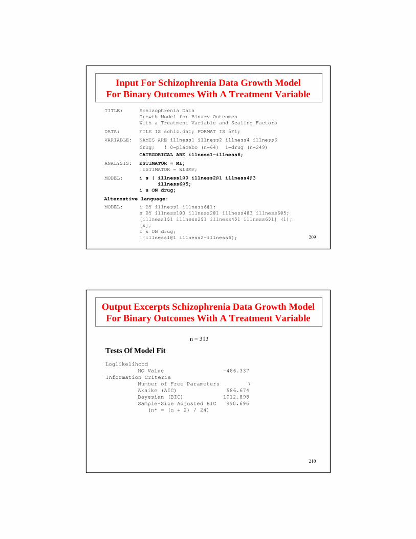
209
Input For Schizophrenia Data Growth ModelFor Binary Outcomes With A Treatment VariableTITLE: Schizophrenia Data
Growth Model for Binary OutcomesWith a Treatment Variable and Scaling Factors
DATA: FILE IS schiz.dat; FORMAT IS 5F1;
VARIABLE: NAMES ARE illness1 illness2 illness4 illness6drug; ! 0=placebo (n=64) 1=drug (n=249)CATEGORICAL ARE illness1-illness6;
ANALYSIS: ESTIMATOR = ML;!ESTIMATOR = WLSMV;
MODEL: i s | illness1@0 illness2@1 illness4@3illness6@5;
i s ON drug;
Alternative language:
MODEL: i BY illness1-illness6@1;s BY illness1@0 illness2@1 illness4@3 illness6@5;[illness1$1 illness2$1 illness4$1 illness6$1] (1);[s];i s ON drug;!{illness1@1 illness2-illness6};
210
Tests Of Model Fit
LoglikelihoodHO Value -486.337
Information CriteriaNumber of Free Parameters 7Akaike (AIC) 986.674Bayesian (BIC) 1012.898Sample-Size Adjusted BIC 990.696
(n* = (n + 2) / 24)
Output Excerpts Schizophrenia Data Growth ModelFor Binary Outcomes With A Treatment Variable
n = 313

211
I ONDRUG -0.429 0.825 -0.521 -0.156 -0.063
S ONDRUG -0.651 0.259 -2.512 -0.684 -0.276
I WITHS -0.925 0.621 -1.489 -0.353 -0.353
InterceptsI 0.000 0.000 0.000 0.000 0.000S -0.555 0.255 -2.182 -0.583 -0.583
ThresholdsILLNESS1$1 -5.706 1.047 -5.451ILLNESS2$1 -5.706 1.047 -5.451ILLNESS4$1 -5.706 1.047 -5.451ILLNESS5$1 -5.706 1.047 -5.451
Residual VariancesI 7.543 3.213 2.348 0.996 0.996S 0.838 0.343 2.440 0.924 0.924
Estimates S.E. Est./S.E. Std StdYXSelected Estimates
Output Excerpts Schizophrenia Data Growth ModelFor Binary Outcomes With A Treatment
Variable (Continued)
212
Fitzmaurice, G.M., Laird, N.M. & Ware, J.H. (2004). Applied longitudinal analysis. New York: Wiley.
Gibbons, R.D. & Hedeker, D. (1997). Random effects probit and logistic regression models for three-level data. Biometrics, 53, 1527-1537.
Hedeker, D. & Gibbons, R.D. (1994). A random-effects ordinal regression model for multilevel analysis. Biometrics, 50, 933-944.
Muthén, B. (1996). Growth modeling with binary responses. In A. V. Eye, & C. Clogg (Eds.), Categorical variables in developmental research: methods of analysis (pp. 37-54). San Diego, CA: Academic Press. (#64)
Muthén, B. & Asparouhov, T. (2002). Latent variable analysis with categorical outcomes: Multiple-group and growth modeling in Mplus. Mplus Web Note #4 (www.statmodel.com).
Further Readings On Growth Analysis With Categorical Outcomes
213
References(To request a Muthén paper, please email [email protected].)
Analysis With Longitudinal DataIntroductoryBollen, K.A. & Curran, P.J. (2006). Latent curve models. A structural
equation perspective. New York: Wiley.Collins, L.M. & Sayer, A. (Eds.) (2001). New methods for the analysis of
change. Washington, D.C.: American Psychological Association.Curran, P.J. & Bollen, K.A. (2001). The best of both worlds: Combining
autoregressive and latent curve models. In Collins, L.M. & Sayer, A.G. (Eds.) New methods for the analysis of change (pp. 105-136). Washington, DC: American Psychological Association.
Duncan, T., Duncan S. & Strycker, L. (2006). An introduction to latent variable growth curve modeling. Second edition. Lawrence Erlbaum: New York.
Goldstein, H. (2003). Multilevel statistical models. Third edition. London: Edward Arnold.
214
Jennrich, R.I. & Schluchter, M.D. (1986). Unbalanced repeated-measures models with structured covariance matrices. Biometrics, 42, 805-820.
Laird, N.M., & Ware, J.H. (1982). Random-effects models for longitudinal data. Biometrics, 38, 963-974.
Lindstrom, M.J. & Bates, D.M. (1988). Newton-Raphson and EM algorithms for linear mixed-effects models for repeated-measures data. Journal of the American Statistical Association, 83, 1014-1022.
Littell, R., Milliken, G.A., Stroup, W.W., & Wolfinger, R.D. (1996). SAS system for mixed models. Cary NC: SAS Institute.
McArdle, J.J. & Epstein, D. (1987). Latent growth curves within developmental structural equation models. Child Development, 58, 110-133.
McArdle, J.J. & Hamagami, F. (2001). Latent differences score structural models for linear dynamic analyses with incomplete longitudinal data. In Collins, L.M. & Sayer, A. G. (Eds.), New methods for the analysis of change (pp. 137-175). Washington, D.C.: American Psychological Association.
Meredith, W. & Tisak, J. (1990). Latent curve analysis Psychometrika, 55, 107-122.
References (Continued)

215
References (Continued)Muthén, B. (1991). Analysis of longitudinal data using latent variable models
with varying parameters. In L. Collins & J. Horn (Eds.), Best methods for the analysis of change. Recent advances, unanswered questions, future directions (pp. 1-17). Washington D.C.: American Psychological Association.
Muthén, B. (2000). Methodological issues in random coefficient growthmodeling using a latent variable framework: Applications to the development of heavy drinking. In Multivariate applications in substance use research, J. Rose, L. Chassin, C. Presson & J. Sherman (eds.), Hillsdale, N.J.: Erlbaum, pp. 113-140.
Muthén, B. & Khoo, S.T. (1998). Longitudinal studies of achievement growth using latent variable modeling. Learning and Individual Differences. Special issue: latent growth curve analysis, 10, 73-101.
Muthén, B. & Muthén, L. (2000). The development of heavy drinking and alcohol-related problems from ages 18 to 37 in a U.S. national sample. Journal of Studies on Alcohol, 61, 290-300.
Muthén, B. & Shedden, K. (1999). Finite mixture modeling with mixtureoutcomes using the EM algorithm. Biometrics, 55, 463-469.
216
References (Continued)Rao, C.R. (1958). Some statistical models for comparison of growth curves.
Biometrics, 14, 1-17.Raudenbush, S.W. & Bryk, A.S. (2002). Hierarchical linear models:
Applications and data analysis methods. Second edition. Newbury Park, CA: Sage Publications.
Singer, J.D. (1998). Using SAS PROC MIXED to fit multilevel models, hierarchical models, and individual growth models. Journal of Educational and Behavioral Statistics, 23, 323-355.
Singer, J.D. & Willett, J.B. (2003). Applied longitudinal data analysis. Modeling change and event occurrence. New York, NY: Oxford University Press.
Snijders, T. & Bosker, R. (1999). Multilevel analysis: An introduction to basic and advanced multilevel modeling. Thousand Oakes, CA: Sage Publications.
Tucker, L.R. (1958). Determination of parameters of a functional relation by factor analysis. Psychometrika, 23, 19-23.
217
References (Continued)Advanced
Albert, P.S. & Shih, J.H. (2003). Modeling tumor growth with random onset. Biometrics, 59, 897-906.
Brown, C.H. & Liao, J. (1999). Principles for designing randomized preventive trials in mental health: An emerging development epidemiologic perspective. American Journal of Community Psychology, special issue on prevention science, 27, 673-709.
Brown, C.H., Indurkhya, A. & Kellam, S.K. (2000). Power calculations for data missing by design: applications to a follow-up study of lead exposure and attention. Journal of the American Statistical Association, 95, 383-395.
Collins, L.M. & Sayer, A. (Eds.), New methods for the analysis of change. Washington, D.C.: American Psychological Association.
Curran, P.J., Muthén, B., & Harford, T.C. (1998). The influence of changes in marital status on developmental trajectories of alcohol use in young adults. Journal of Studies on Alcohol, 59, 647-658.
Duan, N., Manning, W.G., Morris, C.N. & Newhouse, J.P. (1983). Acomparison of alternative models for the demand for medical care. Journal of Business and Economic Statistics, 1, 115-126.
218
References (Continued)Ferrer, E. & McArdle, J.J. (2004). Alternative structural models for
multivariate longitudinal data analysis. Structural Equation Modeling, 10, 493-524.
Fitzmaurice, G., Davidian, M., Verbeke, G. & Molenberghs, G. (2008). Longitudinal Data Analysis. Chapman & Hall/CRC Press.
Klein, A. & Moosbrugger, H. (2000). Maximum likelihood estimation of latent interaction effects with the LMS method. Psychometrika, 65, 457-474.
Khoo, S.T. & Muthén, B. (2000). Longitudinal data on families: Growth modeling alternatives. In Multivariate applications in substance use research, J. Rose, L. Chassin, C. Presson & J. Sherman (eds), Hillsdale,N.J.: Erlbaum, pp. 43-78.
Miyazaki, Y. & Raudenbush, S.W. (2000). A test for linkage of multiple cohorts from an accelerated longitudinal design. Psychological Methods, 5, 44-63.
Moerbeek, M., Breukelen, G.J.P. & Berger, M.P.F. (2000). Design issues for experiments in multilevel populations. Journal of Educational and Behavioral Statistics, 25, 271-284.

219
References (Continued)
Muthén, B. (1996). Growth modeling with binary responses. In A.V. Eye & C. Clogg (eds), Categorical variables in developmental research: methods of analysis (pp. 37-54). San Diego, CA: Academic Press.
Muthén, B. (1997). Latent variable modeling with longitudinal and multilevel data. In A. Raftery (ed), Sociological Methodology (pp. 453-380). Boston: Blackwell Publishers.
Muthén, B. (2004). Latent variable analysis: Growth mixture modeling and related techniques for longitudinal data. In D. Kaplan (ed.), Handbook of quantitative methodology for the social sciences (pp. 345-368). Newbury Park, CA: Sage Publications.
Muthén, B. & Curran, P. (1997). General longitudinal modeling of individual differences in experimental designs: A latent variable framework for analysis and power estimation. Psychological Methods, 2, 371-402.
Muthén, B. & Muthén, L. (2000). The development of heavy drinking and alcohol-related problems from ages 18 to 37 in a U.S. national sample. Journal of Studies on Alcohol, 61, 290-300.
220
References (Continued)Muthén, L.K. and Muthén, B. O. (2002). How to use a Monte Carlo study to
decide on sample size and determine power. Structural Equation Modeling, 4, 599-620.
Olsen, M.K. & Schafer, J.L. (2001). A two-part random effects model for semicontinuous longitudinal data. Journal of the American Statistical Association, 96, 730-745.
Raudenbush, S.W. (1997). Statistical analysis and optimal design for cluster randomized trials. Psychological Methods, 2, 173-185.
Raudenbush, S.W. & Liu, X. (2000). Statistical power and optimal design for multisite randomized trials. Psychological Methods, 5, 199-213.
Roeder, K., Lynch, K.G., & Nagin, D.S. (1999). Modeling uncertainty in latent class membership: A case study in criminology. Journal of the American Statistical Association, 94, 766-776.
Satorra, A. & Saris, W. (1985). Power of the likelihood ratio test in covariance structure analysis. Psychometrika, 51, 83-90.
Related Documents