GROWTH EFFECTS OF URBAN-RURAL AND INTRA-REGIONAL LINKAGES ON COUNTIES AND COMMUNITIES IN THE U.S. BY JOANNA PAULSON GANNING DISSERTATION Submitted in partial fulfillment of the requirements for the degree of Doctor of Philosophy in Regional Planning in the Graduate College of the University of Illinois at Urbana-Champaign, 2010 Urbana, Illinois Doctoral Committee: Assistant Professor Bumsoo Lee, Chair Assistant Professor Katherine Baylis Professor Geoffrey Hewings Professor Sara McLafferty

Welcome message from author
This document is posted to help you gain knowledge. Please leave a comment to let me know what you think about it! Share it to your friends and learn new things together.
Transcript
GROWTH EFFECTS OF URBAN-RURAL AND INTRA-REGIONAL LINKAGES ON COUNTIES AND COMMUNITIES IN THE U.S.
BY
JOANNA PAULSON GANNING
DISSERTATION
Submitted in partial fulfillment of the requirements
for the degree of Doctor of Philosophy in Regional Planning in the Graduate College of the
University of Illinois at Urbana-Champaign, 2010
Urbana, Illinois
Doctoral Committee: Assistant Professor Bumsoo Lee, Chair Assistant Professor Katherine Baylis Professor Geoffrey Hewings Professor Sara McLafferty

ii
Abstract
This dissertation investigates the population growth effects of urban-rural and intra-regional
linkages in the United States. This dissertation follows the three paper format. The first paper
(Chapter 2) investigates the construct reliability of a nodality-based spatial structure scheme for
U.S. metropolitan regions. Using a broad literature review of the relationships between
monocentrism, polycentrism, and economic and demographic variables, I develop hypotheses
regarding theoretical characteristics of monocentric and polycentric regions. I test these
hypotheses using data from regions defined by the nodality-based spatial structure scheme as
monocentric or polycentric. In general, I find that while the drivers of monocentricity are well
understood in the literature and are reflected in the empirically classified monocentric regions,
our theoretical understanding of and our ability to detect polycentricity are not as robust. This
underscores the need to investigate further the growth effects of urban-rural and intra-regional
linkages. In the second paper (Chapter 3) I investigate the growth effects in non-metropolitan
places of growth in proximate Metropolitan Statistical Areas. This chapter concludes that while
commuting plays a critical role in delivering the benefits of urban growth to non-metropolitan
places, economic linkages and commodity flows likely play a much more significant role.
Additionally, there is evidence that non-metropolitan places develop to suit the demands of the
nearest city, rather than participating in more global markets, though much future work could be
done in this area. In the third paper (Chapter 4) I investigate spatial heterogeneity in the
relationship between commuting and migration in a broad region around Chicago. This chapter
supports earlier research findings that population deconcentration is driving the spatial expansion
of economic activity, but that the drivers of that deconcentration vary significantly across space.

iii
Acknowledgements
This project would not have been possible without the support of several people. I owe
much gratitude to my advisor, Professor Bumsoo Lee, for reading drafts of each chapter and
providing constructive feedback. Many thanks also to my committee members, Professors Kathy
Baylis, Geoff Hewings, and Sara McLafferty, who provided substantial guidance. I must also
thank Professor Courtney Flint for her incredible support of me, in so many ways, over the past
four years. I am also thankful for the support of Melissa Zavala in the final formatting of this
document.
On a more personal level, I would not be where I am today without my family, from
those who have gone before me down to the toddlers who greet the world with such wonder. I
dedicate this dissertation to you.
This work was supported in part through the Rural Sociological Society’s Dissertation
Research Award and through the Creative Research grant from University of Illinois College of
Fine and Applied Arts.

iv
Table of Contents
Chapter 1: Introduction ................................................................................................................... 1
1.1 Theoretical Context of the Research ..................................................................................... 3
1.2 Empirical Context of the Research ....................................................................................... 9
1.3 Conceptual Layout of the Dissertation ............................................................................... 12
1.4 Bibliography ....................................................................................................................... 15
Chapter 2: Spatial Structure in U.S. Metropolitan Statistical Areas: Metrics and Theory ........... 19
2.1 Introduction ......................................................................................................................... 19
2.2 Classifying Nodal Spatial Structure in the U.S. .................................................................. 21
2.3 Spatial Structure and Theory .............................................................................................. 26
2.4 The Model ........................................................................................................................... 32
2.5 Results and Discussion ....................................................................................................... 35
2.6 Conclusion .......................................................................................................................... 38
2.7 Bibliography ....................................................................................................................... 39
Chapter 3: Spread and Backwash Effects for Non-metropolitan Communities in the U.S. ......... 44
3.1 Introduction ......................................................................................................................... 44
3.2 Background on Spread-Backwash Concept ........................................................................ 45
3.3 Empirical Specification and Data ....................................................................................... 51
3.4 Results and Discussion ....................................................................................................... 56
3.5 Conclusion .......................................................................................................................... 62

v
3.6 Bibliography ....................................................................................................................... 64
Chapter 4: Detecting and Specifying Spatial Heterogeneity in Commuting Patterns .................. 68
4.1 Introduction ......................................................................................................................... 68
4.2 Analytical Framework ........................................................................................................ 72
4.3 Background ......................................................................................................................... 73
4.4 Chicago, IL MSA Study Region ......................................................................................... 77
4.5 Econometric Analysis ......................................................................................................... 83
4.6 Data ..................................................................................................................................... 88
4.7 Results ................................................................................................................................. 91
4.8 Conclusion .......................................................................................................................... 96
4.9 Bibliography ....................................................................................................................... 99
Chapter 5: Conclusion................................................................................................................. 105
5.1 Summary of Chapters ....................................................................................................... 105
5.2 Synthesis ........................................................................................................................... 107
5.3 Closing .............................................................................................................................. 109
Appendix ..................................................................................................................................... 110
1
Chapter 1: Introduction
In economic development planning, approaches can be broken into three broad groups:
people-based, place-based, and sector- or industry-based. Each of the three has specific strengths
and weaknesses, and each has been trumpeted loudly in different eras of fashion within the
literature. After more than a decade of fervor for sector-based approaches to economic
development (initiated most notably in Porter, 1990), there is a resurgence of place-based
research (e.g. Partridge and Rickman, 2005, 2006, and 2008). The most basic, sound, underlying
truth that beckons scholars back to this thread of research can be summarized easily: “The
wellbeing of people in the countryside is closely inter-linked with that of their urban cousins,
whether an asset or a liability” (Partridge, Bollman, Olfert, and Alasia, 2007, p. 128).
An even-handed treatment of economic development should acknowledge that there are
valid, even critical factors of all three (people-, place-, and sector-based) perspectives that act in
both causing and improving economic development problems. Take, for example, the empirical
starting point used in Moss, Jack, and Wallace (2004): structural change in the agricultural sector
had decreased the economic viability of farming households in Northern Ireland. To sustain
homesteads, many households turned to commuting to mid- and large-sized cities. Their paper
focuses on commuting, but an economic intervention for these households could revolve around
place (improving transportation routes to major employment centers), people (starting workforce
training programs for farmers), or sector (increasing investments in agricultural technology to
make the industry more globally competitive).
As scholars expand their focus beyond the sector-based strategies that have dominated
research, the potential to move place-based research forward is greater than ever.
Technologically, the ability to specify more complete models and spatial models of development

2
has advanced dramatically. For instance, where scholars were previously by technological
capacity to models of single, sub-state regions, we now can model hundreds of regions
simultaneously in some applications. This allows increased capacity to push toward an
understanding of principles rooted in theory and generalizability. When generalized
understanding is developed, then local, contextualized information can be used to better tailor the
theoretically-driven models. Additionally, the menu of spatial econometrics methods continues
to expand. Theoretically, the years spent focused on sector-based development enrich our ability
to study place-based approaches more holistically. Today’s scholars better understand the roles
of education and on amenities that attract creative workers (i.e. Florida, 2002) and the roles that
worker education and creativity play in making industries and sectors competitive.
In the chapters that follow, I study two key mechanisms by which counties and
communities grow based on linkages to metropolitan places: spread-backwash effects and
complementary-substitutive commuting. Both mechanisms are rooted in place-based theories of
economic development, and both are influenced theoretically by an understanding of critical
elements of sector-based development, such as the importance of investment by metropolitan
companies in non-metropolitan production, attractiveness of various characteristics of cities, and
the differences in education levels between places within a region. I have undertaken both based
on a belief in placed-based approaches to economic development and a focus on building a
research agenda using spatial econometrics and regional science methods. Additionally, I have
undertaken a measurement and analysis of regional spatial structure. In the course of that
analysis, I build a body of theory which is used through the dissertation and provides a measure
of regional spatial structure which is incorporated in testing the two aforementioned mechanisms
of population change.
3
The remainder of this chapter outlines the theoretical and empirical contexts for the
research and provides a conceptual diagram of the dissertation. The dissertation follows in the
three-paper format, with the first paper following as chapter two. By measuring a spatial
structure scheme and testing its validity in a U.S. context, this paper sets up background material
for chapters three and four. This was done in the belief, and seeming logic, that metropolitan
regional spatial structure would clearly affect the ability of non-metropolitan residents to access
cities and gain employment within them. Chapter three explores the spread-backwash
mechanism of non-metropolitan community-level population growth. Chapter four studies
county-level commuting over time in regard to migration in a region with a strongly
heterogeneous mix of urban and rural, metropolitan and non-metropolitan parts to assess the
changing nature of population change at the metropolitan fringe as the spatial extent of economic
activity pushes outward. Chapter five summarizes and synthesizes chapters two through four
and concludes the dissertation.
1.1 Theoretical Context of the Research
This dissertation connects two areas of research in the field of regional economic
planning, regional (place-based) development policies and rural-urban interdependencies. Both
areas constitute large sub-fields for research within planning. In this section I will briefly
summarize the relevant research agendas of both areas as they relate to this dissertation. The
theory specific to the growth mechanisms studied in the dissertation is given in each substantive
chapter.

4
Regional Development Policies
The massive domain of economic development planning can be broken down into three
sub-areas: people-, place- and industry- based development theories. I am proposing research
that focuses on places and consequently on place-based development. Controversy surrounds the
appropriateness of such strategies, and the arguments on either side are convincing. Consider that
the whole of neoclassical economics argues against place-based policies, of which regional
policy is a type, since all places will eventually converge through the market. Contrast that with
the reality of places like Appalachia. This sub-section provides a brief review of the theoretical
arguments for regional policies, since the justification of them underlies my proposed research.
The picture that scholars have painted of lagging regions provides multiple avenues to
argue for place-based policies. Duncan (1999) and Black et al. (2005) describe lagging regions as
places with selective out-migration, deterioration of public services, and in the case of Duncan
(1999), not only the economic, but the social ramifications of those changes. In the case of
selective out-migration, place-based policies can target places where there is excess labor, where
income levels are low, or place-based amenities are few (Cumberland, 1971). All of these factors
encourage selective out-migration of residents, which further decreases, in a cycle of cumulative
causation, the competitiveness of a place.
Myrdal (1957) describes cumulative causation as a process in which the loss of industry
causes a decrease in the tax base, after which places cannot maintain their levels of public
service. As those levels decrease, more companies seek better business environments elsewhere.
The provision of public services is seen as both a key component in overcoming regional poverty
and an eligible target for place-based strategies. Place-based policies are necessary to combat the

5
place-based problems of public service provision and maintain regional competitiveness
(Cumberland, 1971).
As Duncan (1999) documents, rural poverty has social ramifications as well. Duncan
documents corruption and nepotism, but there are other social effects. As a community declines,
the sense of place inherent in that place may also decline. One can argue that sense of place is a
public good, which consequently deserves public funds to maintain (Bolton, 1992). The place-
based market imperfections that cause the decline of places must be addressed through place-
based strategies (Bolton, 1992).
Another social cause and consequence of rural poverty is remoteness. As Litcher and
Johnson (2007) find, remoteness is linked to persistent rural poverty and social isolation that
precludes the most isolated from opportunities. Partridge and Rickman (2006) also argue that
remoteness and isolation are causes of rural poverty. Remoteness is a function of location; place-
based problems merit place-based solutions. Concentrating economic development initiatives at
isolated places reduces poverty efficiently, as there is little competition from commuters or
migrants for the funds. Blank (2005) also reviews the relationship between local characteristics
and development, with a discussion of the necessity of both people- and place-based policies.
Aside from the characterizations of lagging regions, there are theoretical, economic
arguments for place-based approaches to economic development. New Economic Geography
(NEG) can be used to argue for place-based strategies. According to NEG, externalities are
linked to market size, and externalities are part of the key to economic agglomeration and
divergence of regions (Fingleton and Lopez-Bazo, 2006; Krugman, 1991). Place-based strategies
can help rural areas experience agglomeration and knowledge spillovers, which are critical to
development in this theoretical perspective (Partridge and Rickman, 2006).
6
The economic arguments of cumulative causation and the Verdoorn Law (that there is a
strong positive association between the growth of productivity and efficiency and the rate of
growth in the scale of activities) are strong and convincing arguments for regional policies.
Kaldor (1970) argues, with reference to the Verndoorn Law, that wage differences within a
country are limited due to labor mobility, so efficiency wages will accrue in regions with higher
productivity, thus starting a cycle of cumulative causation. This counters the neoclassical
economics argument that regions will converge.
Some weaknesses of place-based policies merit noting. Some of the specific
shortcomings include: aid always comes at some opportunity cost to other places, assistance can't
be effectively targeted, place-based policies are always overtly political, the local public sector
has to be important, the government has no concern for those they do not target, and regional
policies target the average resident of the region, which may not be the appropriate target
(Bolton, 1992). Based on a literature review, Partridge and Rickman (2006) point out that place-
based policies “induce the disadvantaged not to migrate to localities with better employment
opportunities, which creates a culture of dependency in the region” (2006, p. 12; see also Shaw,
1986).
Rural-Urban Interdependency
Within the field of regional development planning, there are several literatures that
describe the importance of the linkages between central cities or cities and communities or
regions. Three theories in particular seem closely related to the proposed research: central place
theory, growth-pole theory, and spread-backwash theories. These three theories share the
hypothesis that development beyond the central city relies on the economic power of the city.
7
While measuring the linkages of places to the city, this relationship is the focus of this
dissertation.
Central place theory has its roots in mid-twentieth century German planning research by
Walter Christaller (1966). Christaller develops a theory of central goods and their market areas,
given economic rationality. Central places can be distinguished based on their traffic, market,
and sociopolitical spatial patterns. The traffic principle is based on transportation lines
connecting the central places, forming a linear system. Christaller’s theories of market-based
spatial structure are reminiscent of Losch's hexagons (1938). The sociopolitical system deals
with borders between political areas, with administrative areas, and other organizational/political
barriers or systems which would change the system of places. These three systems of
classification overlap, making delineation of central cities technically complicated. The traffic
and market systems are economic; the separation theory is political and less rational. Central
place theory hypothesizes that increasing technology will boost the existing central places and
call new ones into being to fulfill the increase in supply. Christaller empirically sketches a
system of central places in southern Germany using measures he devises and describes, namely,
the number of telephone connections beyond the national per capita rate.
Growth pole theory is generally attributed to the work of Francois Perroux. A
development pole, which is related to a growth pole, can be defined as a "growth inducing unit
coupled with its surrounding environment” (Perroux, 1988). The theory suggests that a
propulsive industry in one location can encourage growth outward from that location. As Perroux
explains, "To generalize: the dynamic enterprise exerts an induction effect upon another
enterprise in a given environment for a more or less short or long period" (1988, p. 67). One of
the largest criticisms of growth pole theory is that the terminology was not originally defined
8
clearly and was not prescriptive enough for clear implementation. Perroux and other published
papers trying to clarify the nuanced differences between related terms (Perroux 1988; Parr 1999a
and 1999b), but empirically these efforts never yielded clear success.
Empirically, in an effort to prove that the Appalachian Regional Commission (ARC)
wasn’t just pork, ARC leaders tried to implement a growth pole oriented development strategy.
The politics involved in dividing development funding among 13 states, however, proved to be
too much for the non-prescriptive nature of the theory. "For the sake of conformity, the
Commission designated the various state-determined growth centers as regional, primary, or
secondary centers" (Wood, 2001, p. 556). These didn't mean much ultimately. Just over 2/3 of all
ARC counties were designated as growth centers, which was grossly out of line with theory and
meant that funds were not concentrated. As one politician explained, "'I don't know exactly what
a growth center is, but I know there is at least one in each congressional district'" (Wood, 2001,
p. 556). Growth centers covered about 90% of region's residents. The strategy was eventually
abandoned in 1983 after failing to arrive at a coherent means of implementing the growth pole
approach.
A third literature on urban-rural dependency is the spread-backwash literature. Spread-
backwash effects were outlined by Myrdal (1957) and Hirschman (1959) in the late 1950s.
Generally, spread effects are the positive effects of urban proximity for communities, and
backwash effects are the negative consequences of proximity. According to Hirschman, the most
important spread effect is the purchase and investments of the affluent region in the outlying
region. The negative (backwash) effects include migration to the more developed region,
especially of the more skilled and trained workers, and weak production in the outlying region,
caused by superior competition in the more developed area. At its simplest, spread and backwash

9
can be measured by either population change or income change as a function of distance to the
nearest city. Gaile (1980) frames the evolution of spread and backwash concepts. More recent
notable contributions have come from Carlino and Mills (1987) and Boarnet (1994), who
explored county level income and population growth.
1.2 Empirical Context of the Research
In addition to the ARC implementation of growth pole theory, one thread of empirical
research relating to intra-regional linkages is of the relationship between highways (one measure
of linkages) and county-level productivity or growth (Aschauer, 1989; Chandra and Thompson,
2000; Garcia-Mila and McGuire, 1992; Rephann and Isserman, 1994). Aschauer (1989) provides
some context for studying intra-regional linkages and productivity, by testing the relationship
between non-military public capital stock, a core of infrastructure, and changes in productivity in
the private US economy. Chandra and Thompson (2000) and Rephann and Isserman (1994)
measure income change in counties that have gained highway development compared to a
control group of counties. Garcia-Mila and McGuire (1992) study "the productive contribution of
publicly provided goods and services, in particular, highways and education" (p. 229). Though
the proposed research focuses on a different measure of intra-regional linkage (commuting), the
relevancy of the findings on highway development are clear.
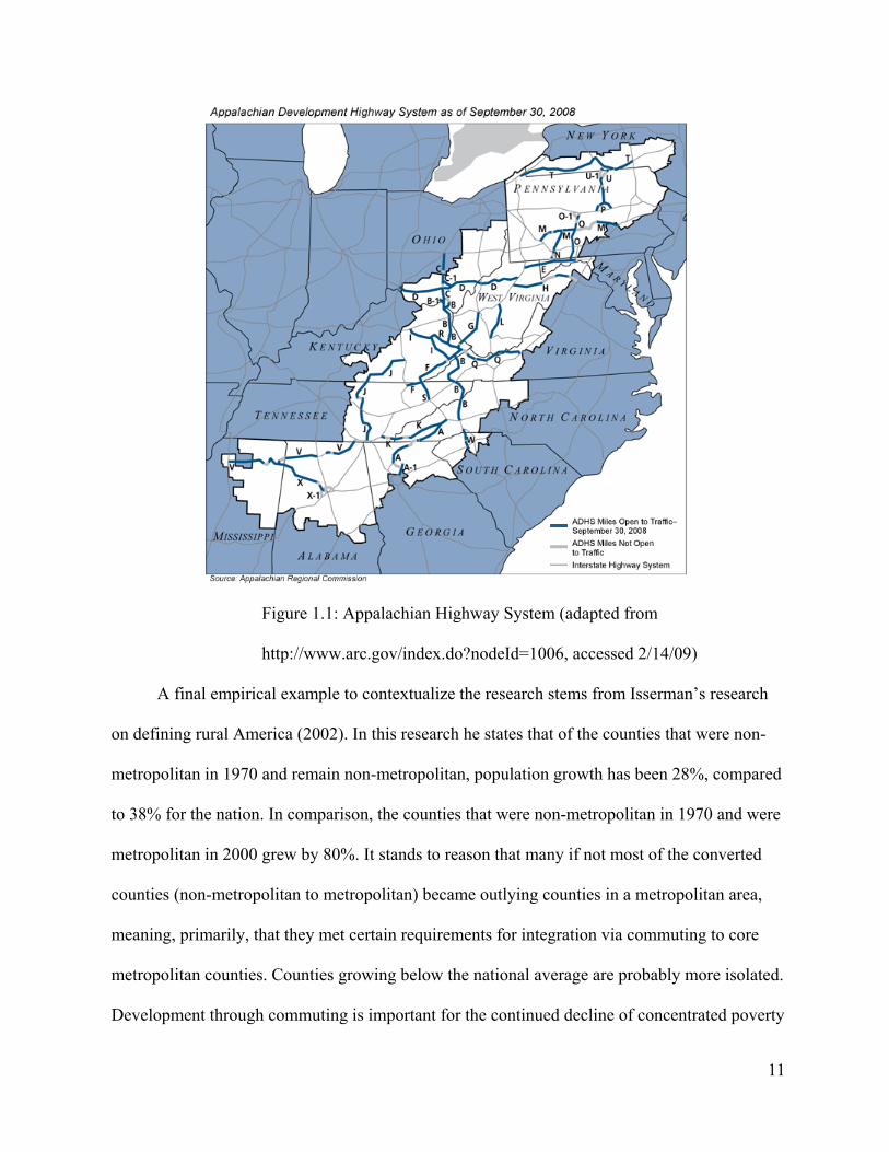
An empirical example of the importance of the theories of intra-regional linkages can be
seen in the Appalachian Regional Commission’s focus on highway development. The
Appalachian Highway System (Figure 1.1), which connects rural areas to more densely settled
cities, has a constant dollar economic return rate of 8.29% and has had a multiplier effect of 1.32
in the region. As of September 2006, over 2,300 miles of the Appalachian Highway System were
10
complete. Funding to continue building through 2009 is authorized through the Safe,
Accountable, Flexible, and Efficient Transportation Equity Act: A Legacy for Users (Wilbur
Smith Associates, 1998).
Isserman and Rephann (1995) provide a convincing argument that without the
Appalachian Regional Commission (ARC), which is a place-based approach to development, the
Appalachian counties would not have grown as quickly as they have. Cumberland (1971) and
Bolton (1992) provide a summary of the arguments for and against regional policies.
Access to cities is an important fixture of the economy across the U.S. In 2000, 17% of
nonmetropolitan residents commuted to central cities and suburbs, and 90% of suburban
residents worked in metropolitan areas (suburbs or central cities) (Pisarski, 2006, p. 48). As it
related to rural and small town development, commuting outside of the home county is most
common among smaller counties (Pisarski, 2006, p. 49); intra-regional linkages are critical for
these places. Commuter flows also showed strong regionality. In 2000, only 7% of central city
residents and 10% of suburban residents worked outside of their home metro area. The strength
of intra-regional flows thus validates the study of intra-regional linkages rather than inter-
regional linkages for effects on population growth.
11
Figure 1.1: Appalachian Highway System (adapted from
http://www.arc.gov/index.do?nodeId=1006, accessed 2/14/09)
A final empirical example to contextualize the research stems from Isserman’s research
on defining rural America (2002). In this research he states that of the counties that were non-
metropolitan in 1970 and remain non-metropolitan, population growth has been 28%, compared
to 38% for the nation. In comparison, the counties that were non-metropolitan in 1970 and were
metropolitan in 2000 grew by 80%. It stands to reason that many if not most of the converted
counties (non-metropolitan to metropolitan) became outlying counties in a metropolitan area,
meaning, primarily, that they met certain requirements for integration via commuting to core
metropolitan counties. Counties growing below the national average are probably more isolated.
Development through commuting is important for the continued decline of concentrated poverty
12
in rural places and for exposing rural children to opportunities away from home (see Lichter and
Johnson, 2007). For these isolated counties, spread effects through commuting are even more
critical.
1.3 Conceptual Layout of the Dissertation
The central theme of this dissertation is reflected in its title: the growth effects of intra-
regional and urban-rural linkages. The approach I take to researching along that theme is shown
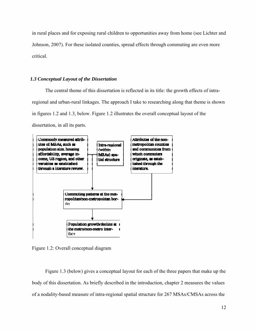
in figures 1.2 and 1.3, below. Figure 1.2 illustrates the overall conceptual layout of the
dissertation, in all its parts.
Figure 1.2: Overall conceptual diagram
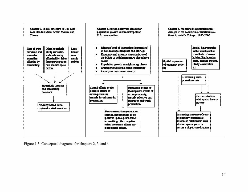
Figure 1.3 (below) gives a conceptual layout for each of the three papers that make up the
body of this dissertation. As briefly described in the introduction, chapter 2 measures the values
of a nodality-based measure of intra-regional spatial structure for 267 MSAs/CMSAs across the

13
U.S. and tests its validity given a large body of theory regarding household location choice and
the drivers of monocentrism and polycentrism. In chapter 3 I measure spread-backwash effects
on population growth for 2,170 non-metropolitan U.S. Census designated places for the period
2000-2007. Spread effects are, in simple terms, the positive effects of urban proximity, most
notably the investment in production in outlying areas. Backwash effects are the negative
effects of urban proximity, including weak production and selective out-migration. My
approach is novel in the geographic breadth for a U.S. study and in its focus on conceptual
measurement and comparison, as well as its use of commuting data for weighting.
In chapter 4 I investigate the changing relationship between commuting and migration for
a 65-county region surrounding Chicago, IL. Informally, a great amount of residential turnover
and population growth has been observed at the urban-rural fringe areas within this region.
Based on previous empirical work (Renkow and Hoover, 2000) and the untested observation of a
concomitantly expanding spatial range of economic activity, it was thought that workers were
moving from traditional suburbs into more distant suburbs and commuting to jobs that were
suburbanizing to the traditional suburban areas. However, population growth and commuting
have changed unevenly across space. This paper sets out to explore theoretical mechanisms and
use that theory to build on the empirical modeling of the spatial heterogeneity observed in the
commuting-migration relationship across the region in 2000.
Taken together, these three chapters contribute to the central theme of this dissertation, as
given in Figure 1.2. Chapter 5 synthesizes the findings of chapters 2 through 4 around that
theme.
14
Figure 1.3: Conceptual diagrams for chapters 2, 3, and 4
15
1.4 Bibliography
Aschauer, David Alan. 1989. Is public expenditure productive? Journal of Monetary Economics
23: 177-200.
Black, Dan, Terra McKinnish, and Seth Sanders. 2005. The economic impact of the coal boom
and bust. Economic Journal 115(50): 449-476.
Blank, Rebecca M. 2005. Poverty, policy, and place: how poverty and policies to alleviate
poverty are shaped by local characteristics. International Regional Science Review 28(4):
441-464.
Boarnet, Marlon G. 1994. An empirical model of intrametropolitan population and employment
growth. Papers in Regional Science 73(2): 135-152.
Bolton, Roger. 1992. 'Place prosperity vs people prosperity' revisited: An old issue with a new
angle. Urban Studies 29(2): 185-203.
Carlino, Gerald A., and Edwin S. Mills. 1987. The determinants of county growth. Journal of
Regional Science 27(1): 39-54.
Chandra, Amitabh, and Eric Thompson. 2000. Does public investment affect economic activity?
Evidence from the rural interstate highway system. Regional Science and Urban Economics
30: 457-490.
Christaller, Walter. 1966. Central places in southern Germany. Trans. Carlisle W. Baskin.
Englewood Cliffs, NJ: Prentice-Hall.
Cumberland, John H. 1971. Issues in U.S. regional development experience. In Regional
development: Experiences and prospects in the United States of America, pg. 6-20. Paris:
Mouton.

16
Duncan, Cynthia M. 1999. Worlds apart: Why poverty persists in rural America. New Haven:
Yale University Press.
Fingleton, Bernard, and Enrique Lopez-Baro. 2006. Empirical growth models with spatial
effects. Papers in Regional Science 85(2): 177-198.
Gaile, G. L. 1980. The spread-backwash concept. Regional Studies 14(1): 15-25.
Garcia-Milà, Teresa, and Therese J. McGuire. 1992/6. The contribution of publicly provided
inputs to states' economies. Regional Science and Urban Economics 22(2): 229-241.
Hirschman, Albert O. 1959. Interregional and international transmission of economic growth.
Chapter 10 in The strategy of economic development. New Haven: Yale University Press.
Isserman, Andrew, and Terance Rephann. 1995. The economic effects of the Appalachian
regional commission. Journal of the American Planning Association 61(Summer).
Kaldor, Nicholas A. 1970. The case for regional policies. Scottish Journal of Political Economy
17: 337-348.
Krugman, Paul. 1991. Increasing returns and economic geography. Journal of Political Economy
99(3): 483-499.
Lichter, D.T. and K.M. Johnson. 2007. The Changing Spatial Concentration of America’s Rural
Poor Population. Rural Sociology 72: 331-358.
Losch, August. 1938. The nature of economic regions. Southern Economic Journal 5(1): 71-78.
Moss, Joan, Claire Jack, and Michael Wallace. 2004. Employment location and associated
commuting patterns for individuals in disadvantaged rural areas in northern ireland.
Regional Studies 38(2): 121-136.
Myrdal, Gunnar. 1957. The drift towards regional economic inequalities in a country. In
Economic theory and under-developed regions, pg. 23-38. London: Gerald Duckworth.

17
Parr, John B. 1999. Growth-pole strategies in regional economic planning: A retrospective view.
part 1. Origins and advocacy. Urban Studies 36(7): 1195-1215.
———. 1999. Growth-pole strategies in regional economic planning: A retrospective view. part
2. Implementation and outcome. Urban Studies 36(8): 1247-1268.
Partridge, Mark D., Ray D. Bollman, Rose Olfert, and Alessandro Alasia. 2007. Riding the wave
of urban growth in the countryside: Spread, backwash, or stagnation? Land Economics
83(2): 128-152.
Partridge, Mark D., and Dan S. Rickman. 2008. Distance from urban agglomeration economies
and rural poverty. Journal of Regional Science 48(2): 285-310.
———. 2006. The geography of American poverty. Kalamazoo, MI: W.E. Upjohn Institute for
Employment Research.
———. 2005. High- poverty nonmetropolitan counties in America: Can economic development
help? International Regional Science Review 28(4): 415-440.
Porter, Michael. 1990. The competitive advantage of nations. New York: The Free Press.
Perroux, Francois. 1988. The pole of development's new place in a general theory of economic
activity. In Regional economic development: Essays in honour of Francois Perroux., eds.
Benjamin Higgins, Donald J. Savoie, pg. 48-76. Boston: Unwin Hyman.
Pisarski, Alan E. 2006. “Commuting in America III.” Washington, D.C.: Transportation
Research Board of the National Academies.
Renkow, Mitch, and Dale Hoover. 2000. Commuting, migration, and rural-urban population
dynamics. Journal of Regional Science 40(2).

18
Rephann, Terance, and Andrew Isserman. 1994. New highways as economic development tools:
An evaluation using quasi-experimental matching methods. Regional Science and Urban
Economics 24: 723-751.
Shaw, R. Paul. 1986. Fiscal versus traditional market variables in Canadian migration. Journal of
Political Economy 94(3): 648.
Wood, Lawrence E. 2001. From theory to implementation: An analysis of the Appalachian
regional commission's growth center policy. Environment & Planning A 33: 551-565.
Wilbur Smith Associates. 1998. “Appalachian Development Highways Economic Impact
Studies.” Prepared for the Appalachian Regional Commission. Available online:
http://www.arc.gov/images/reports/wsa/wsa-final.pdf. Accessed 1/13/09.

19
Chapter 2: Spatial Structure in U.S. Metropolitan Statistical Areas: Metrics and Theory
2.1 Introduction
Through the middle and end of the twentieth century, many Americans aspired to have an
attractive home with a lawn, within reasonable driving distance to an urban center. This national
ideal cultivated an image of a worker commuting from any one of a dozen identical suburbs to a
region’s city. In the 21st century that image is quickly changing, to an image of a region with
multiple nodes, edge cities, and complex spatial patterns. Examples abound. Consider Tysons
Corner, outside of Washington, DC. Tysons Corner was once a mere crossroads, then later a
budding suburb of the nation’s capital. Today Tysons Corner is the seventeenth largest central
business district in the country. Tysons Corner has become a viable economic engine, an
economic center of its own right. The irony is that Tysons Corner remains unincorporated, parts
of two other towns’ postal areas; we continue to treat it as a piece of land between other suburbs
(Fogg, 2007). This slight is indicative of a broader failure to recognize the vast and significant
changes, including economic ones that are evident in the spatial structure of regions.
As these changes have come to bear on American society, the study of spatial structure
and commuting has gained popularity among social scientists. The spatial structure of regions is
often measured by commute time or distance for workers originating in suburbs versus central
cities (e.g. Gordon, Kumar, and Richardson, 1989), counties, Census tracts, or even block
groups. Scholars have investigated a wide range of economic and social processes through the
lens of spatial structure: the development of regional economies (Van der Laan, 1998), the
influence of changing prosperity and employment growth on commuting (Schwanen et al.,
2004), the relationship between spatial structure and transit mode choice (Schwanen et al., 2004),
20
the drivers of the non-metropolitan turnaround (Henry et al., 2001; Renkow and Hoover, 2000),
the choice to commute or move and the subsequent socioeconomic and community development
issues (Eliasson et al., 2003), the impacts of housing segregation (Gottlieb and Lentnek, 2001;
Shen, 2000), and the role of planning and planning goals in influencing the commuting patterns
of various groups (Rouwendal and Meijer, 2001).
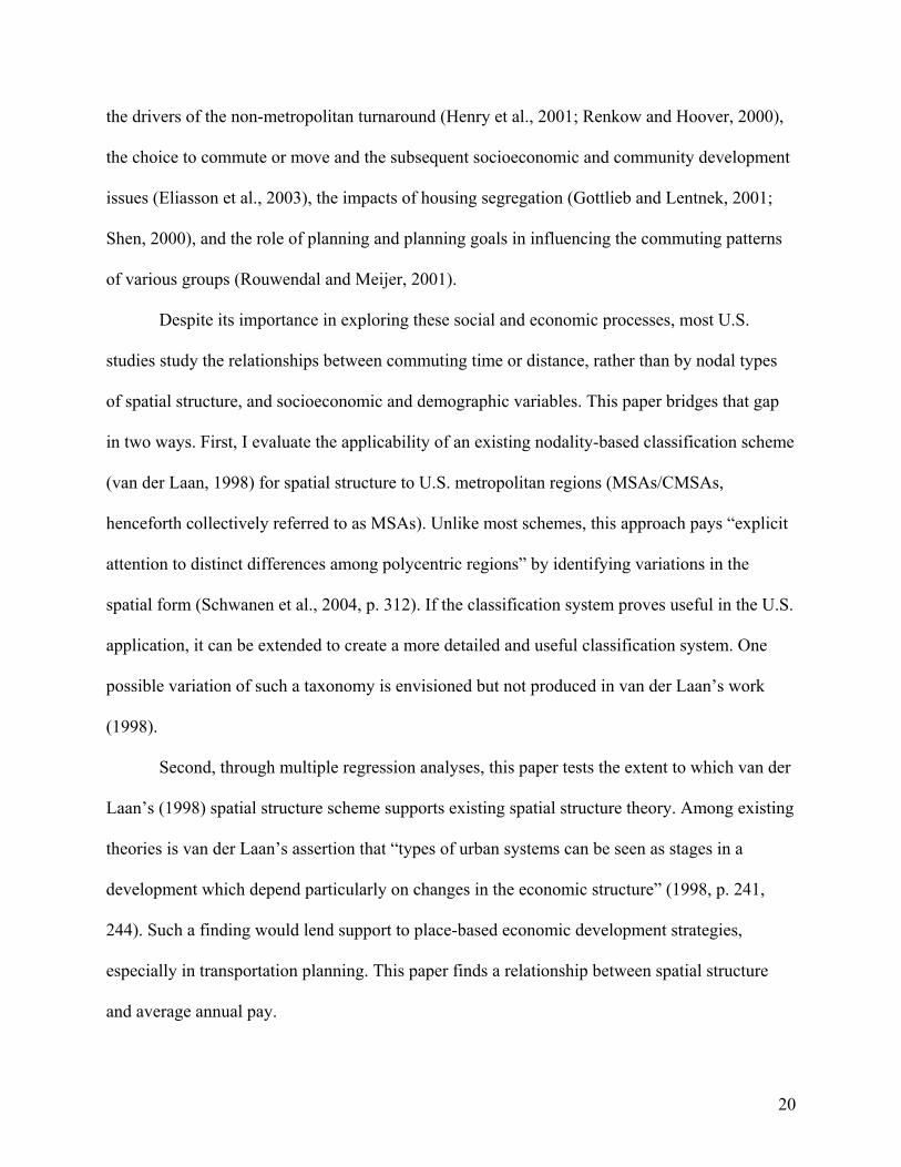
Despite its importance in exploring these social and economic processes, most U.S.
studies study the relationships between commuting time or distance, rather than by nodal types
of spatial structure, and socioeconomic and demographic variables. This paper bridges that gap
in two ways. First, I evaluate the applicability of an existing nodality-based classification scheme
(van der Laan, 1998) for spatial structure to U.S. metropolitan regions (MSAs/CMSAs,
henceforth collectively referred to as MSAs). Unlike most schemes, this approach pays “explicit
attention to distinct differences among polycentric regions” by identifying variations in the
spatial form (Schwanen et al., 2004, p. 312). If the classification system proves useful in the U.S.
application, it can be extended to create a more detailed and useful classification system. One
possible variation of such a taxonomy is envisioned but not produced in van der Laan’s work
(1998).
Second, through multiple regression analyses, this paper tests the extent to which van der
Laan’s (1998) spatial structure scheme supports existing spatial structure theory. Among existing
theories is van der Laan’s assertion that “types of urban systems can be seen as stages in a
development which depend particularly on changes in the economic structure” (1998, p. 241,
244). Such a finding would lend support to place-based economic development strategies,
especially in transportation planning. This paper finds a relationship between spatial structure
and average annual pay.
21
The remainder of this paper is arranged in four sections. The first section describes the
spatial structure scheme used in this paper, describes the methods used to apply it to the U.S.,
and briefly presents the results of that application. The second section reviews theory of spatial
structure and various socioeconomic and demographic variables. The third section introduces the
multiple regression models and variables used to test the applicability of the theory to van der
Laan’s spatial structure scheme in the U.S. The final section presents and discusses the results of
those models.
2.2 Classifying Nodal Spatial Structure in the U.S.
Van der Laan’s classification scheme relies on the ability of the researcher to identify
streams of commuters into and out of central cities using Dutch commuting data. Fortunately,
similar information can be ascertained in the U.S., with some imposition of definitions, using the
Census Transportation Planning Package 2000 (CTPP 2000). The method is based on flows into
and out of the central city and suburbs, not all flows into and out of the city or metropolitan
region. Similarly, flows originating in the central city and ending outside of the MSA are
excluded. The VDL approach has the benefit of identifying not only regions with centralized or
dispersed spatial structures, but also the flow of workers among the nodes within regions. The
downside of this approach is that it does not reveal the number and relative significance of the
nodes.
Van der Laan’s typology (1998, henceforth VDL), which underlies both his own work
and Schwanen et al. (2004) is mechanically straightforward. Van der Laan represents the
typology in a two-by-two matrix:

22
Table 2.1: VDL Classification Scheme
From/to Central
city
Suburbs
Suburbs N1:
traditional
commuting
cross-
commuting
Central
city
locally
employed
N2:
reverse
commuting
Where:
Nodality-1 (N1) = (ICC/ICD)*100
Where ICC = sum of flows from intra-MSA suburbs to the MSA’s central city
ICD = sum of flows between all places in the MSA
Nodality-2 (N2) = (OCC/OCD)*100
Where OCC = sum of flows from the central city to intra-MSA suburbs
OCD = sum of flows between all places in the MSA
ICD = OCD
N1 represents flows to the central city from the suburbs (defined as Census designated
places that are not the central city, defined below) as a percent of all place-to-place flows. N2 is
concerned with commuters who live in the central city and work in the suburbs. The sum of the
23
four quadrants in Table 2.1 represents all commuters that begin and end their journey to work in
places within the MSA. This approach ignores commuter flows that begin or end outside of the
MSA, and those that begin or end in non-places within the MSA. The flows that either begin or
end in non-places are significant. For example, in the Winchester, VA-WV MSA, only 14.7% of
intra-regional commuters begin and end the journey to work in Census designated places. At the
other end of the spectrum, in the San Jose-Sunnyvale-Santa Clara, CA MSA, 93.7% of workers
begin and end their commutes in Census designated places. The focus of the spatial structure
scheme under study here is nodality, or the joint distribution of people and jobs. Areas that have
workers but are not Census designated places, by definition, are not places with significant local
economies. Consequently, these observations are not considered in this study. The ICD and OCD
measures given above use the sum of flows that both begin and end in Census designated places,
rather than the total sum of all intra-regional commuter flows. An extension of this work could
expand Table 2.1 into a three-by-three grid, where the third row and third column are “non-
places.”
Van der Laan (1998) plots regions according to scores for N1 and N2. The plot is divided
into four unevenly sized quadrants, representing exchange-commuting, central commuting,
decentral commuting, and cross-commuting. Exchange-commuting means that suburban
residents work in the central city and central city dwellers often work in the suburbs. VDL
asserts that central commuting indicates a monocentric or traditional spatial structure, where the
central city attracts workers and the suburbs serve as bedroom communities. Decentral
commuting implies the opposite, that suburbs attract workers from both suburbs and the central
city. Finally, cross-commuting means that many suburban residents work in suburbs (not
necessarily those they live in) and central city residents work in the central city. This is a type of

24
intra-regional dual labor market, meaning that there are two distinct labor markets in the region.
See Schwanen et al. (2003) for illustrative diagrams of the types.
I calculated N1 and N2 for all MSAs for which sufficient data is available (267 of the 276
MSAs defined by the OMB in 19991). Before measuring N1 and N2, one additional step must be
implemented. The VDL scheme relies on measuring commuting into and out of the central city.
The Office of Management and Budget defines central city as the principal city within a region.
Up to two additional cities can be included as central cities if they meet specific criteria (OMB,
2006). In cases where there are two or three central cities in a region, the Census Bureau bases
selection of central cities primarily upon commuting data. However, the VDL scheme does not
allow for measuring flows into multiple central cities within a region, leaving two reasonable
alternatives: use only the principal city or aggregate all central cities into one artificial (and
spatially non-contiguous) central city. I use the principal city as the definition of the central city;
the option of aggregating not only combines areas that are not spatially contiguous, but also
combines places that have distinguishing features, even when the places are spatially contiguous,
as in the case of Champaign and Urbana, Illinois.
Figure 2.1 shows the distribution of MSAs along the measures N1 and N2. The lines are
set at the median point for N1 and N2, following VDL’s example. The medians of N1 and N2 are
lower in Figure 2.1 than in van der Laan’s Dutch data. This may result from the small sample
size in the Dutch data. This might also reflect differences in U.S. and Dutch commuting patterns,
or a difference in MSA/DUS (Daily Urban Systems, the Dutch equivalent of MSAs) definitions
(for instance, the size of the space around a central city that is included in the region, since
MSAs are built from counties and DUSs are not). The N1 median in particular is much lower
1 N1 and N2 values cannot be calculated for Anchorage, AK; Athens, GA; Danville, VA; Enid, OK; Jonesboro, AR; Lawton, OK; Lincoln, NE; Owensboro, KY; Topeka, KS. There are no commuting flows reported between the central cities of these cities and any other place within the MSA.

25
using U.S. data than in the Dutch case. This indicates that U.S. cities are less traditional, relying
less on the flow of suburban workers to the central city than on other, more complex spatial
patterns. This finding seems consistent with the well-documented suburbanization of America.
The extreme outlier in the Decentral quadrant is Clarksville-Hopkinsville, TN-KY. The
outlier in the upper right corner of the Central quadrant is Grand Junction, CO. This means that a
significant share of labor market traffic in Grand Junction is directed from the suburbs to the
central city. As points of reference, the New York City CMSA has an N1 of 0.26 and an N2
value of 0.36, putting it in the Cross Commuting quadrant. Chicago has an N1 value of 12.59 and
an N2 of 8.46, putting it in the Decentral quadrant, but near the median point of both the N1 and
N2 distributions (15.79 and 6.74, respectively).

26
Figure 2.1: Distribution of U.S. MSAs along N1 and N2 measures
2.3 Spatial Structure and Theory
The studies on commuting time and distance provide a rich body of theory on which to
ground a study of spatial structure. This section briefly reviews that literature and reviews the
hypotheses that guide the model presented in the next section. Testing the relationships between
existing theory and the VDL structure will help to ground the structure in the scholarly
discussion on commuting as well as set up a research framework for extending its practical
applications. Because the models (described in the next section) used to test this body of theory

27
use N1 and N2 as dependent variables, hypotheses relating to each theoretical component are
expressed in terms of N1 and N2.
Theory
Spatial Structure—Accessibility and Monocentrism versus Polycentrism
Spatial accessibility generally refers to the ability of workers within a region to access
employment opportunities, though definitions vary. Accessibility has been of key interest in
studying, among other topics, segregation (Gottlieb and Lentnek, 2001), job search models
(Eliasson et al., 2003), and transit choice (Shen, 2000). Studies repeatedly show accessibility’s
significance. Even given different measures and definitions, accessibility influences commuting
patterns, and thus spatial structure, within regions.
Accessibility can be measured in numerous ways. Eliasson et al. (2003) measure intra-
regional accessibility by counting the population of working age within a given area. Shen
(2000) creates scores based on number of jobs, number of workers, automobile ownership, and
impedance functions to measure accessibility for workers who are auto drivers and transit riders.
Cervero and Duncan (2006) count job, retail, and service destinations within a given radius of a
survey respondent’s home. The methods of testing the importance of accessibility also vary, as
the models and methods vary considerably across these cited papers. Regardless, accessibility
remains the most consistently significant explanatory variable in studies involving spatial
structure.
As Cervero and Duncan (2006) quote from Handy and Niemeier (1997), “no one best
approach to measuring accessibility exists; different situations and purposes demand different
approaches” (p. 478, quoting from p. 1181). I use a straightforward measure: the number of
28
vehicles used for commuting divided by the employed population in the region. With increasing
accessibility, regions are expected to be more often multi-nodal, with less local commuting. In
other words, I hypothesize a negative relationship between accessibility and N1 and a positive
relationship with N2.
Gender Studies
Gender has been of interest because men both earn more and commute farther than
women, seemingly irrespective of type of residential location or industry of work (see
MacDonald, 1999). Two theories have emerged to explain women’s commuting patterns relative
to men’s: the Entrapment Theory and the Household Responsibility Theory.
The Entrapment Theory focuses on women’s inability to travel as far as men to obtain
more lucrative employment. Women can be entrapped by inaccessibility of transportation (Moss
et al., 2004), by paternalistic social structures (Little and Austin, 1996), by a concentration of
local industries, typically in the service sector or textiles (Cristaldi, 2005), or by discriminatory
wages in better-paying, farther away industries (Carlson and Persky, 1999). Van Ommeren et al.
(1999) support the theory in their finding that marriage restricts the frequency with which
women change jobs.
The Household Responsibility Theory (HRT) contends that women hold household and
family responsibilities that keep them close to home. Theorized causal mechanisms include
encouragement to work near the home community (Moss et al., 2004; Turner and Niemeier,
1997), an oppressive and paternalistic rural social structure that forces women to accept multiple
responsibilities (Little and Austin, 1996), and child rearing responsibilities (McQuaid, Greig, and
Adams, 2001). Others (e.g. White, 1986) find no support for the HRT. Phimister, Vera-Toscano,

29
and Weersink (2002), for example, see no barriers to rural women’s mobility, arguing that
socioeconomic standing of rural women is consistent with the observed trend toward smaller
commutes.
As a measure of the role of gender in a region’s spatial structure, I include labor force
participation by gender. The literature on gender indicates that where the female labor force
participation rate is high, the average commute time will be shorter. Since Schwanen et al.
(2004) find that average commute time is shorter in monocentric cities, I anticipate finding
higher female labor force participation rates in Central-type cities (i.e. a positive relationship
with N1 and negative with N2). I also anticipate that the female labor force participation rate will
be positively correlated with accessibility.
Industry and Occupation
The literature relating commute time and/or distance to industry and occupation is largely
inconclusive. Perhaps using commute time and distance are poor metrics for testing the
relationship between spatial structure and regional economics. Nevertheless, two broad theories
find support across the literature. First, commuting time and efficiency (degree of cross-hauling)
by occupation and industry vary (Artis et al., 2000; Gessaman and Sisler, 1976; Gober et al.,
1993; Krout, 1983; Moss et al., 2004; O’Kelly and Wook, 2005).
Second, the service sector tends to draw from local workers rather than in-commuters
(Artis et al., 2000; Moss et al., 2004; Krout, 1983; Turner and Neimeier, 1997). Service sector
firms may have a preference for local workers (Turner and Neimeier, 1997). Another explanation
is that service sector positions tend to have low barriers to entry and flexible work schedules,
making the jobs attractive to women who are entrapped or who manage household

30
responsibilities (Moss et al., 2004). Finally, Artis et al. find empirical evidence for Simpson’s
claim “that labour market size increases with the worker’s qualification level” (p. 1444, 2000).
Academics find less room for agreement when studying other industries and sectors. For
example, Clemente and Summers (1975) found that within a manufacturing firm there is no
relationship between occupation and commuting distance. More recently, Moss et al. (2004) and
Artis et al. (2000) find that more educated workers tend to commute more.2 However, Moss et al.
find that professional workers commute shorter distances (at a non-significant level), while Artis
et al. find that professional workers commute more in order to maximize use of skills and thus
income. See also McQuaid et al. (2001) and Fernandez and Su (2004).
To test the relationship between socioeconomics and spatial structure, I use average
compensation per job rather than economic structure variables such as percent employment in
the service sector. I do this for two reasons. First, it is difficult to identify demographically-
driven impacts on spatial structure from employment data in broadly-defined economic sectors.
Incomes and occupations within the service sector, for instance, vary widely. Employment
statistics for more narrowly defined industries suffer from non-disclosure, sometimes even for
small MSAs. Second, van der Laan hypothesizes a relationship between spatial structure and a
region’s ability to shift to a knowledge-based economy (KBE). KBEs are not characterized by
strong employment in any one industry (e.g. Vence-Deza and Gonzalez-Lopez, 2008). A KBE
works through upgrading multiple industries for higher returns to investment across the local
economy. Using average compensation per job measures this phenomenon better than
employment in broadly-defined industries. The limitation of using average compensation is that
it generally varies with city size and somewhat with region.
2 “Commute more” is measured differently in these two papers—one by time and one by crossing regional borders.
31
Van der Laan (1998) calls Central regions monocentric, non-complex regions.
Consequently, given the theory presented here, I would not expect these regions to have high
levels of average compensation. Theory thus predicts a negative relationship between average
compensation and N1 and a positive relationship with N2.
Urban Integration and Rural Amenities
The inclusion of rural amenities in spatial structure studies allows researchers to
investigate the influence of housing affordability on regional structure in high-amenity areas
(Gober et al., 1993), the potential for commuting to offset rural decline (Moss et al., 2004, see
also Partridge and Rickman, 2005), the role of family in residential location preference (Clark
and Withers, 1999; Davis and Nelson, 1994; Green, 1997; Mok, 2007; Rouwendal and Meijer,
2001), the mechanism driving regional restructuring (Renkow and Hoover, 2000), and the
potential for rural development given expanding metropolitan labor markets (Berry, 1970;
Hazans, 2004).
Rural amenities can be widely construed as the characteristics of a bucolic setting which
entice individuals or households to visit or settle permanently. Each MSA receives a score from
0-100 for rural amenities, which indicates the percentage of places within the MSA which are
rural. Places are categorized as rural using RUCA codes (ERS, 2005) and GIS. Using GIS, I first
locate the Census tract of each place’s centroid. Places within tracts of RUCA codes 4-10 are
counted as “rural” places. I also control for housing affordability to better understand the role of
rural amenities versus income-housing matching. The literature does not set up a clear hypothesis
for the relationship between rural amenities and N1 and N2, or the VDL types. It seems likely
that rural amenity-rich regions would be Central (higher N1, lower N2), since small towns are,

32
theoretically, embraced for home-life qualities, not economic purposes; they are bedroom
communities. In short, places with high levels of rural amenities are not expected to have local
employment structures.
Dual-Income Households
Commutes vary between single workers and workers in two-wage-earner households.
Consequently, spatial structure is expected to vary with household type. The most studied factor
in dual-income commuting is housing preference for households with and without children
(Clark and Withers, 1999; Davis and Nelson, 1994; Green, 1997; Mok, 2007; Rouwendal and
Meijer, 2001). Households with children prefer larger housing in smaller towns, which has
specific implications for spatial structure, though I do not control for the presence of children in
this paper. I measure the impact of dual-income household status by including labor force
participation by marital status. Like rural amenities, the hypothesis stemming from this literature
is unclear, but it seems reasonable to anticipate a positive relationship between the percent of
dual-income households and N1, and a negative relationship with N2.
The dual-income household literature also relates to and enriches the gender-based
literature. For a discussion, see Clark and Withers (1999), Green (1997), Mok (2007), Plaut
(2006), Rouwendal and Meijer (2001), Skaburskis (1997), and van Ommeren (1999).
2.4 The Model
I use ordinary least squares regression to test the theoretical relationships described in the
previous section. The dependent variables are N1 and N2. I use N1 and N2 rather than VDL
33
spatial structure type as dependent variables because the cut-off points between VDL types are
set by the median of N1 and N2, which is somewhat arbitrary and may bias the results.
In addition to the variables drawn from theory, I also control for location using the
Census Bureau’s designations for Division (see Appendix, Figure A1). Division was assigned
according to the location of each MSA’s principal city. Controlling for Census division helps to
control for some of the historic reasons that cities developed differently. For instance, cities like
Philadelphia and Annapolis developed before the automobile, with dense and narrow streets,
while Los Angeles took form with the explosion of the automotive industry in the United States.
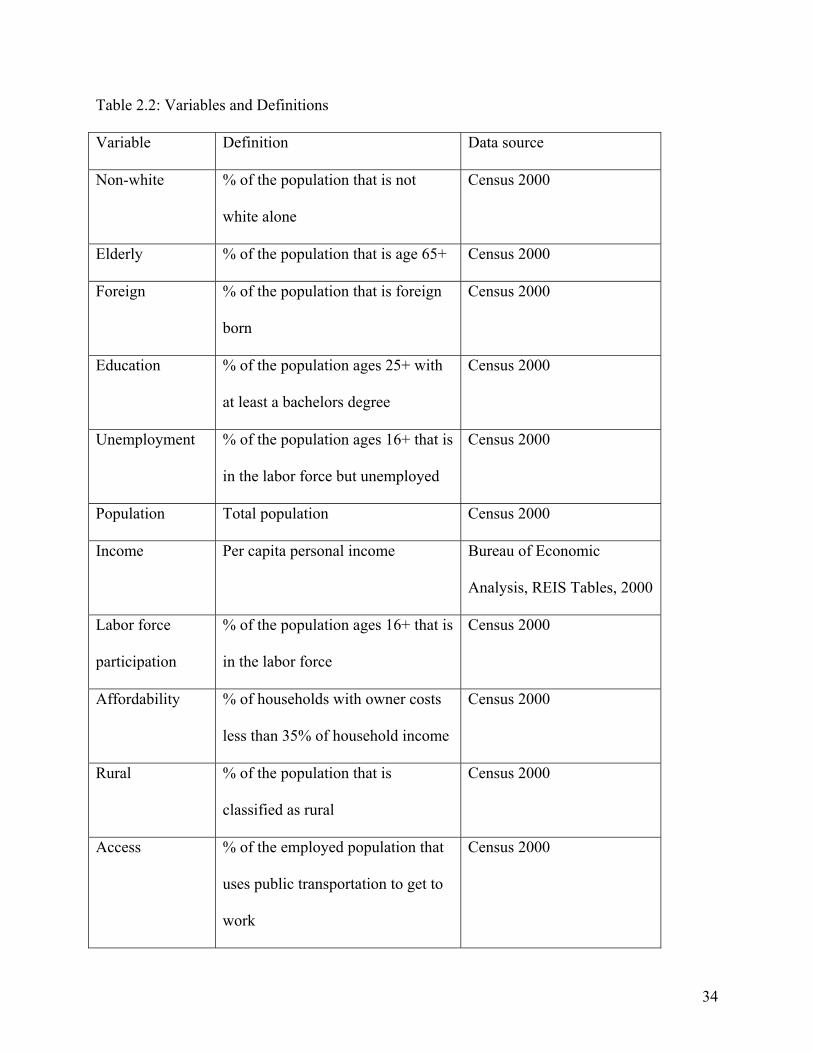
Variables, definitions, and data sources are provided in Table 2.2. All data and conclusions are
drawn at the MSA-level. The right hand side variables are drawn from the 2000 Census and
other data sources from 2000.
I calculated an interaction term for all combinations of dummy and scale variables. The
interaction terms did not strengthen the models and were consequently dropped. Many of the
variables listed in Table 2.2 were highly correlated. To reduce multicollinearity in the model
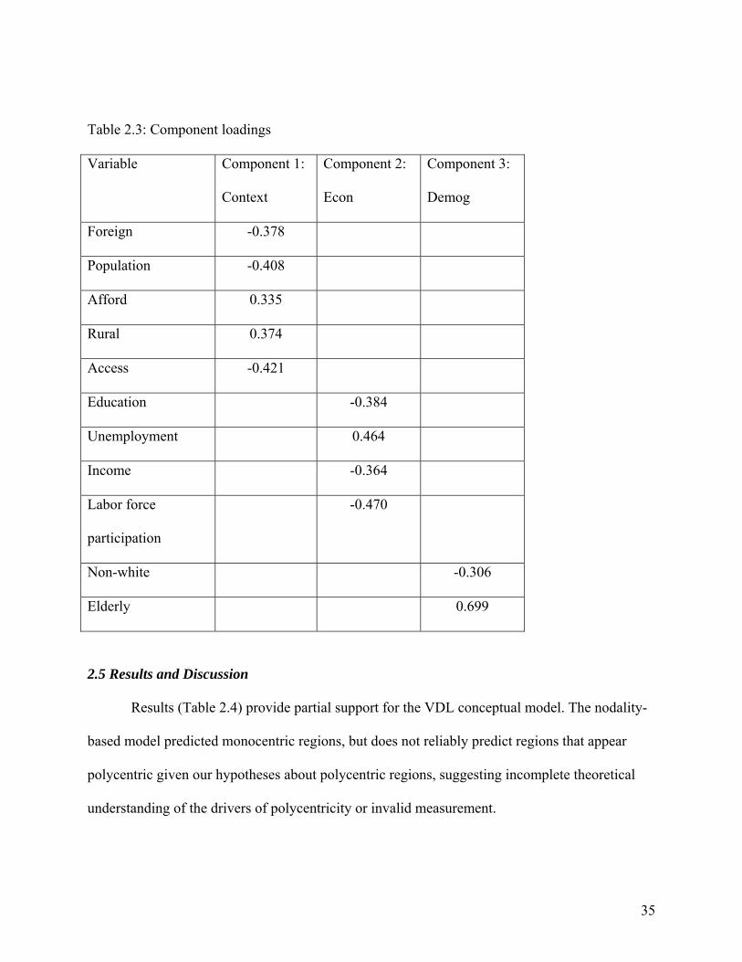
without restricting it to a very small number of variables, I used a principal component analysis
to reduce the explanatory variables into three components. Table 2.3 shows the loadings of each
variable on its most representative component. This is provided to guide interpretation of model
results. The resulting OLS models of N1 and N2 show neither multicollinearity nor
heteroskedasticity.
34
Table 2.2: Variables and Definitions
Variable Definition Data source
Non-white % of the population that is not
white alone
Census 2000
Elderly % of the population that is age 65+ Census 2000
Foreign % of the population that is foreign
born
Census 2000
Education % of the population ages 25+ with
at least a bachelors degree
Census 2000
Unemployment % of the population ages 16+ that is
in the labor force but unemployed
Census 2000
Population Total population Census 2000
Income Per capita personal income Bureau of Economic
Analysis, REIS Tables, 2000
Labor force
participation
% of the population ages 16+ that is
in the labor force
Census 2000
Affordability % of households with owner costs
less than 35% of household income
Census 2000
Rural % of the population that is
classified as rural
Census 2000
Access % of the employed population that
uses public transportation to get to
work
Census 2000
35
Table 2.3: Component loadings
Variable Component 1:
Context
Component 2:
Econ
Component 3:
Demog
Foreign -0.378
Population -0.408
Afford 0.335
Rural 0.374
Access -0.421
Education -0.384
Unemployment 0.464
Income -0.364
Labor force
participation
-0.470
Non-white -0.306
Elderly 0.699
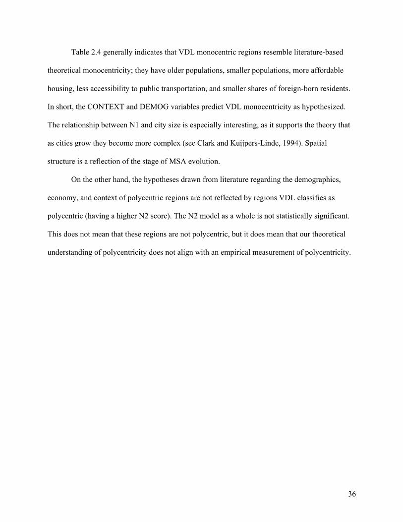
2.5 Results and Discussion
Results (Table 2.4) provide partial support for the VDL conceptual model. The nodality-
based model predicted monocentric regions, but does not reliably predict regions that appear
polycentric given our hypotheses about polycentric regions, suggesting incomplete theoretical
understanding of the drivers of polycentricity or invalid measurement.
36
Table 2.4 generally indicates that VDL monocentric regions resemble literature-based
theoretical monocentricity; they have older populations, smaller populations, more affordable
housing, less accessibility to public transportation, and smaller shares of foreign-born residents.
In short, the CONTEXT and DEMOG variables predict VDL monocentricity as hypothesized.
The relationship between N1 and city size is especially interesting, as it supports the theory that
as cities grow they become more complex (see Clark and Kuijpers-Linde, 1994). Spatial
structure is a reflection of the stage of MSA evolution.
On the other hand, the hypotheses drawn from literature regarding the demographics,
economy, and context of polycentric regions are not reflected by regions VDL classifies as
polycentric (having a higher N2 score). The N2 model as a whole is not statistically significant.
This does not mean that these regions are not polycentric, but it does mean that our theoretical
understanding of polycentricity does not align with an empirical measurement of polycentricity.

37
Table 2.4: Regression analyses of N1 and N2
Estimate Std. Error Signif. Estimate Std. Error Signif.
Intercept 14.8794 2.2805 *** 8.90744 1.32703 ***
CONTEXT 0.8152 0.2802 *** 0.22147 0.16303
ECON ‐0.4227 0.3691 0.02635 0.2148
DEMOG 0.9738 0.3919 ** ‐0.45683 0.22802 **
ESC 2.3641 2.8476 ‐1.78544 1.65705
PCF 3.7797 2.9378 ‐1.51954 1.70954
MNT ‐0.1121 2.7702 ‐2.86045 1.61204 *
WSC ‐0.7855 2.7111 ‐2.97319 1.57763 *
SA 2.929 2.4982 ‐2.75142 1.45374 *
ENC ‐0.9402 2.5557 ‐0.86307 1.48722
MA 0.9751 2.7651 ‐0.16242 1.60907
WNC ‐2.1618 2.7848 ‐2.86298 1.6205 *
Adj. R^2
F‐statistic
P‐value 0.00173
1.66
0.08286
N1 N2
0.0699 0.02657
2.817
* indicates significance at the 0.10 level, ** indicates significance at the 0.05 level, *** indicates significance at the
0.01 level
The bulk of spatial structure research revolves around topics relating to regional
economics. It is therefore most surprising that the economic variables are not statistically
significant in the N1 and N2 models. This suggests that further study, in which one or a few
regions are studied in a time series model, might be an appropriate approach. It seems likely that
a region’s economy and its spatial structure do not develop in perfect tandem. However, without
clear empirical evidence as to which comes first, and at what time lag, constructing a better
specified model will remain difficult.
Surprisingly, the Census Division variables (with New England as the comparison
category) did not strengthen the N1 model, but some are statistically significant in the N2 model.
With New England as the reference Division, all other Divisions carry a negative coefficient for

38
the N2 model, indicating that reverse commuting (central city to suburb) is more common in
New England than elsewhere.
Taken together, the results of N1 and N2 indicate that the VDL approach adequately
measures traditional commuting in a way that is validated by its relationships with explanatory
variables. In other words, the N1 model is significant (though with a very low R-squared value)
and aligns reasonably well with theory. However, the N2 model is not significant at the 0.05
level. This indicates that the VDL conceptual measurement either does not reliably detect
polycentricity, or our theoretical understanding of its drivers is incomplete by a wide margin.
2.6 Conclusion
This paper set out to assess the applicability of a nodality-based spatial structure scheme
to U.S. regions. In sum, the VDL scheme can be measured and applied for U.S. regions. Models
of the VDL spatial structure variables N1 and N2 indicate that the N1 variable, which describes
the traditional suburb-to-central city commuting pattern, is supported fairly well by theory.
However, N2, which would theoretically permit the detection of polycentric regions, finds less
support from theory.
This work suggests that while the straightforward concept of the traditional, monocentric
city can be readily related to contextual, economic and demographic variables, our understanding
of multinodality is less complete. Much work remains to be done in investigating the causal
mechanisms of multinodality and its temporal relationships with economic and demographic
changes. Based on the work of Clark and Kuijpers-Linde and this manuscript, it would seem that
a productive avenue may be the development of more detailed conceptual diagrams of
multinodal cities, from which case studies of cities can be carried out.
39
2.7 Bibliography
Artís, Manuel, Javier Romaní, and Jordi Suriñach. 2000. Determinants of individual commuting
in Catalonia, 1986–91: Theory and empirical evidence. Urban Studies 37(8): 1431-1450.
Berry, Brian J. L. 1970. Labor market participation and regional potential. Growth & Change
1(4): 3.
Carlson, Virginia L., and Joseph J. Persky. 1999. Gender and suburban wages. Economic
Geography 75(1).
Cervero, Robert, and Michael Duncan. 2006. Which reduces vehicle travel more: Jobs-housing
balance or retail-housing mixing? Journal of the American Planning Association 72(4): 475-
490.
Clark, William A. V., and Marianne Kuijpers-Linde. 1994. Commuting in restructuring urban
regions. Urban Studies 31(3): 465-483.
Clark, William A. V., and Suzanne Davies Withers. 1999. Changing jobs and changing houses:
Mobility outcomes of employment transitions. Journal of Regional Science 39(4): 653-673.
Clemente, Frank, and Gene F. Summers. 1975. The journey to work of rural industrial
employees. Social Forces 54(1): 212-219.
Cristaldi, Flavia. 2005. Commuting and gender in Italy: A methodological issue. Professional
Geographer 57(2): 268-284.
Davis, Judy S., and Arthur C. Nelson. 1994. The new 'burbs. The exurbs and their implications
for planning policy. Journal of the American Planning Association 60(1)(Winter): 45.
Economic Research Service. 2005. 2000 Rural-Urban Commuting Area Codes. Available online:
http://www.ers.usda.gov/Data/RuralUrbanCommutingAreaCodes/2000/.
40
Eliasson, Kent, Urban Lindgren, and Olle Westerlund. 2003. Geographical labour mobility:
Migration or commuting? Regional Studies 37(8): 827.
Fernandez, Roberto M., and Celina Su. 2004. Space in the study of labor markets. Annual
Review of Sociology 30(1): 545-569.
Fogg, Alan Arthur. 2007. You say McLean. I say Vienna. Let’s all say Tyson’s. The Washington
Post, February 25, 2007, 2007, sec B08.
Gessaman, Paul, and Daniel Sisler. 1976. Highways, changing land use, and impacts on rural
life. Growth & Change (April 1976): 3-8.
Gober, Patricia, Kevin E. McHugh, and Denis Leclerc. 1993. Job-rich by housing poor: The
dilemma of a western amenity town. Professional Geographer 45(1): 12-20.
Gottlieb, Paul D., and Barry Lentnek. 2001. Spatial mismatch is not always a central-city
problem: An analysis of commuting behaviour in Cleveland, Ohio, and its suburbs. Urban
Studies 38(7): 1161-1186.
Gordon, Peter, Ajay Kumar, and Harry W. Richardson. 1989. Congestion, changing metropolitan
structure, and city size in the United States. International Regional Science Review 12(1):
45-56.
Green, A. E. 1997. A question of compromise? Case study evidence on the location and mobility
strategies of dual career households. Regional Studies 31(7): 641.
Handy, S. and D.A. Niemeier. 1997. Measuring accessibility: An exploration of issues and
alternatives. Environment and Planning A, 29(7): 1175-1194.
Hazans, Mihails. 2004. Does commuting reduce wage disparities? Growth & Change 35(3): 360-
390.
41
Henry, Mark S., Bertrant Schmitt, and Virginie Piguet. 2001. Spatial econometric models for
simultaneous systems: application to rural community growth in France. International
Regional Science Review 24(2): 171-193.
Isserman, A. M. (2002). Defining regions for rural America. Federal Reserve Bank of Kansas
City.
Krout, John. 1983. Intercounty commuting in nonmetropolitan America in 1960 and 1970.
Growth & Change (January 1983): 10-19.
Little, Jo, and Patricia Austin. 1996. Women and the rural idyll. Journal of Regional Studies 12:
101-111.
MacDonald, Heather I. 1999. Women's employment and commuting: Explaining the links.
Journal of Planning Literature 13(3): 267-283.
McQuaid, R. W., M. Greig, and J. Adams. 2001. Unemployed job seeker attitudes towards
potential travel-to-work times. Growth & Change 32(3): 355-368.
Mok, Diana. 2007. Do two-earner households base their choice of residential location on both
incomes? Urban Studies 44(4): 723-750.
Moss, Joan, Claire Jack, and Michael Wallace. 2004. Employment location and associated
commuting patterns for individuals in disadvantaged rural areas in Northern Ireland.
Regional Studies 38(2): 121-136.
Office of Management and Budget. OMB Bulletin 07-01. December 18, 2006. “Update of
statistical area definitions and guidance on their uses.”
http://www.whitehouse.gov/omb/bulletins/fy2007/b07-01.pdf. Accessed 3/26/2008.
42
O'Kelly, Morton E., and Lee Wook. 2005. Disaggregate journey-to-work data: Implications for
excess commuting and jobs -- housing balance. Environment & Planning A 37(12): 2233-
2252.
Partridge, Mark D., and Dan S. Rickman. 2005. High- poverty nonmetropolitan counties in
America: Can economic development help? International Regional Science Review 28(4):
415-440.
Phimister, Euan, Esperanza Vera-Toscano, and Alfons Weersink. 2002. Female participation and
labor market attachment in rural Canada. American Journal of Agricultural Economics
84(12): 210.
Plaut, Pnina O. 2006. The intra-household choices regarding commuting and housing.
Transportation Research Part A: Policy & Practice 40(7): 561-571.
Renkow, Mitch, and Dale Hoover. 2000. Commuting, migration, and rural-urban population
dynamics. Journal of Regional Science 40(2): 261-287.
Rouwendal, Jan, and Erik Meijer. 2001. Preferences for housing, jobs, and commuting: A mixed
logit analysis. Journal of Regional Science 41(3).
Schwanen, Tim, Frans M. Dieleman, and Martin Dijst. 2004. The impact of metropolitan
structure on commute behavior in the Netherlands: A multilevel approach. Growth &
Change 35(3): 304-333.
———. 2003. Car use in the Netherlands Daily Urban Systems: Does Polycentrism Result in
Lower Commute Times? Urban Geography 24(5): 410-430.
Shen, Qing. 2000. Spatial and social dimensions of commuting. Journal of the American
Planning Association 66(1): 68-82.
43
Skaburskis, Andrejs. 1997. Gender differences in housing demand. Urban Studies 34(2): 275-
320.
Turner, T., and D. Niemeier. 1997. Travel to work and household responsibility: New evidence.
Transportation 24: 397-419.
U.S. Bureau of Labor Statistics. 2000. Quarterly Census of Employment and Wages.
Washington, D.C.
U.S. Bureau of the Census. 2000. Census 2000. Washington, D.C.
U.S. Department of Transportation, Bureau of Transportation Statistics. Census Transportation
Planning Package 2000. Washington, D.C.
van der Laan, Lambert. 1998. Changing urban systems: An empirical analysis at two spatial
levels. Regional Studies 32(3): 235-247.
van Ommeren, Jos, Piet Rietveld, and Peter Nijkamp. 1999. Impacts of employed spouses on
job-moving behavior. International Regional Science Review 22(4): 54-68.
Vence-Deza, X., and M. González-López. 2008. Regional concentration of the knowledge-based
economy in the EU: Towards a renewed oligocentric model? European Planning Studies
16(4): 557-578.
White, M. J. 1986. Sex differences in urban commuting patterns. American Economic Review 76:
332-368.

44
Chapter 3: Spread and Backwash Effects for Non-metropolitan Communities in the U.S.
3.1 Introduction
The rural idyll provides an image of a self-sustaining, economically viable countryside
dotted with close-knit, picturesque communities. Like all ideals, however, the image is flawed.
“The wellbeing of people in the countryside is closely inter-linked with that of their urban
cousins, whether an asset or a liability” (Partridge, Bollman, Olfert, and Alasia, 2007, p. 128).
For those studying rural and regional development then, urban-rural linkage models can provide
critical information about the pathways by which cities both help and hinder communities.
As Partridge et al. (2007) point out, the concept of urban-rural linkages is not a new one.
Current interest stems from ongoing developments in the literature, especially within the subject
areas of new economic geography, deconcentration and restructuring, rural amenities,
demographic effects on regional spatial structure, and urban sprawl. For rural and regional
development, information about the economic relationship between communities and urban
centers can provide meaningful information for transportation development projects. Highway
development is a success story of the Appalachian Regional Commission’s work. Research
relating urban growth and rural and regional development can only make those projects more
fiscally efficient.
The notion that rural and regional development is tied, both positively and negatively, to
urban development is commonly referred to as spread-backwash effects. In short, this paper tests
three methods of measuring spread and backwash effects of 276 Metropolitan Statistical
Areas/Consolidated Metropolitan Statistical Areas (collectively henceforth referred to as MSAs)
on population growth in 2,170 non-metropolitan Census places across the U.S. from 2000-2007.
45
Traditionally, spread-backwash effects are measured as a function of income growth, population
growth and the distance between the non-metropolitan place and the nearest city. This paper
challenges the notion that only the nearest city matters, suggesting that instead, non-metropolitan
places’ growth can be influenced by multiple cities. To test that hypothesis, I measure population
growth via three separate conceptual approaches, as a function of the characteristics of: the
nearest city, multiple cities weighted by their inverse-distance to the non-metropolitan place, and
multiple cities weighted by the commuting flow from each non-metropolitan place to the MSA.
Though theory suggests that an inverse-distance weighting of multiple cities is preferable, the
strength of the nearest city model indicates that non-metropolitan economies evolve to serve
proximate demand. A more elaborate specification of the inverse-distance model is suggested.
3.2 Background on Spread-Backwash Concept
The spread-backwash concept began in the 1950s with the nearly simultaneous
publications of Hirschman (1959) and Myrdal (1957). Hirschman’s “trickling down” effects are
conceptually analogous to Myrdal’s spread effects—those effects of urban influence which
benefit the outlying areas. According to Hirschman, the most important of these effects is the
purchase and investments of the affluent region in the outlying region. The negative (backwash
or polarization) effects include migration to the more developed region, especially of the more
skilled and trained workers, and weak production in the outlying region, caused by superior
competition in the more developed area. Hirschman acknowledges in a footnote that Myrdal
published his spread-backwash ideas first, though he criticizes Myrdal’s emphasis on cumulative
causation, which Hirschman believes implies too dismal an ending for the outlying areas
(Hirschman, 1959, p. 187).
46
At its simplest, spread and backwash can be measured by either population change or
income change as a function of distance to the nearest city and growth in that city. Regardless of
a town’s economic structure or amenities, it is possible for the community to grow if its workers
have access to the city when there is excess labor at home, or to access the urban service and
recreation sectors. As Partridge et al. (2007) describe in detail, the concept of population growth
effects that are attributable to distance only can be referred to as the urban distance discount
(UDD). In addition to the UDD, several factors may influence spread and backwash effects, most
notably, the income growth rate and population growth rate of the nearest city (or set of cities
which influences each non-metropolitan place), and the characteristics of the non-metropolitan
community itself.
The transition of these ideas from theory to models began in earnest in the late 1980s
when Carlino and Mills (1987) explored determinants of growth at the county level. Intra-
metropolitan growth was taken up by Boarnet’s (1994) econometric model of spread-backwash
effects introducing the spatial lag of population and employment change. Over time the model
has been extended, most notably by Henry, Barkley, and Boa (1997), who find that spread
effects are greater when outlying places are near a decentralized urban node; Henry, Schmitt,
Kristensen, Barkley, and Bao (1999), who find that spread effects depend on size of local labor
zones near the outlying area; and Rey and Boarnet (1998). This work is tied closely to studies of
agglomeration and spillovers and to questions of industrial location and production. Gaile (1980)
reviews the concepts related to spread-backwash effects and the theoretical and empirical
approaches taken for its study.
The early papers on spread-backwash effects limited their focus to small regions, such as
communities within South Carolina (Henry, Barkley, and Bao, 1997), or parts of France (Henry,
47
Schmitt, and Piguie, 2001). The first, and to the author’s knowledge only, study to incorporate a
larger study area is Partridge et al. (2007), which considers spread and backwash effects in
Canada from 1981-2001. Most papers also rely on ordinal measurements of rural proximity,
rather than using continuous variables such as distance. See Partridge et al. (2007, p. 129-130)
for a fuller discussion of this advancement.
The following are two of many approaches to studying rural and regional development to
which the spread-backwash framework can apply. First, Moss, Jack, and Wallace (2004) begin
their work with the notion that when rural economies face structural economic changes, workers
can sustain their communities via commuting to proximate urban labor markets. This is a special
case of spread effects of urban growth. Though the non-metropolitan place’s population may not
grow, if communities are sustained then population sizes also will not decrease at the rate that
would be observed if commuting were not possible. Second, Berry (1970) describes the gradient
of income change with increasing distance from an urban center given different parameters. He
hypothesizes that rural areas fare better when they have access to multiple metropolitan labor
markets and when the cities to which they have access are larger. His hypotheses, like Moss et al.
(2004) rely on the spread effects of urban areas. Furthermore, he provides some hypotheses of
the traits of the urban centers that will influence the degree of the spread-backwash effects.
U.S. Context and Sample
Given basic descriptive statistics about U.S. non-metropolitan places, it is likely that non-
metropolitan residents can commute to proximate urban labor markets and perhaps often have
access to multiple cities. The vast majority of non-metropolitan places are relatively close to an
MSA. Fifty-nine percent of the communities studied in this paper (sample size is 2,170 non-

48
metropolitan places, defined below) are within fifty miles of the primary central city of an MSA,
and 13 percent are within 25 miles. This contradicts the image of a non-metropolitan American
that is truly isolated (though there are 155 places that are more than 100 miles from a central
city). Despite the proximity, these places are in non-metropolitan counties, meaning that there is
not a strong commuting tie to the metropolitan central county of the MSA. Both Moss et al.
(2004) and Berry (1970) present notions of non-metropolitan residents that may still be accurate;
there is room for increased commuting to cities, pushed by either excess labor supply or by
structural change.
Figure 3.1: Distribution of distance (miles) between communities and nearest MSA
This paper builds on the spread-backwash literature in three ways. Primarily, I test the
hypothesis that non-metropolitan places are influenced by multiple cities by comparing the
Minimum distance to a central city
Fre
qu
en
cy
0 200 400 600 800
01
00
20
03
00
40
0

49
results of models constructed with three different conceptual measurements. Theoretical
arguments can be made for any of the three conceptual measurements: nearest city, inverse-
distance, and commuting-weighted. The nearest city approach follows the traditional view of the
city; atomistic and monocentric. Discussions of more complex spatial structures are much newer
than the concepts of spread and backwash.
Allowing cities to influence non-metropolitan growth in proportion to the inverse
distance between each city and non-metropolitan place has the great strength of allowing
multiple cities to influence a non-metropolitan place. It also acknowledges that goods can be
brought to market in a city even when the non-metropolitan residents do not commute to the
given city; consider grain shipments through the Midwest, for example. This approach captures
spread and backwash effects that affect both commuters and businesses, but does not include any
weighting for variation in infrastructure provision which enables both commuting and freight
movement. In this paper I introduce a proxy for infrastructure provision. The primary weakness
of this approach is that it likely permits influence from too wide a sample of cities.
The third approach, commuting-weighted, also has the strength of permitting influence
from multiple cities. Unlike the inverse distance approach, using commuting flows allows the
selection of the unique set of cities that is likely to influence growth in a given non-metropolitan
place via commuting. The weakness of this approach is that it ignores the ability to ship goods to
markets situated beyond the commuting sphere, thus underestimating spread effects from
investment in manufacturing, which is a key theoretical spread effect. This approach likely
underestimates the set of cities that influence non-metropolitan growth. It could be argued that
cities within a pre-selected distance band could be permitted to influence non-metropolitan
place-level growth in a model. However, that approach would over-estimate for some and under-
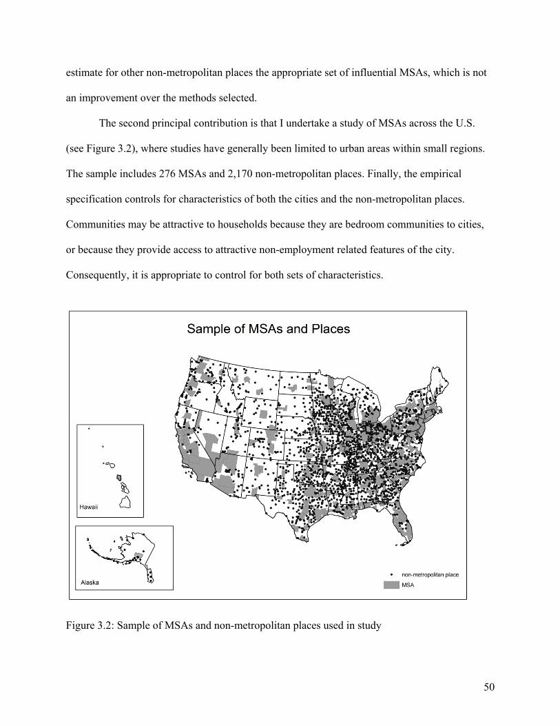
50
estimate for other non-metropolitan places the appropriate set of influential MSAs, which is not
an improvement over the methods selected.
The second principal contribution is that I undertake a study of MSAs across the U.S.
(see Figure 3.2), where studies have generally been limited to urban areas within small regions.
The sample includes 276 MSAs and 2,170 non-metropolitan places. Finally, the empirical
specification controls for characteristics of both the cities and the non-metropolitan places.
Communities may be attractive to households because they are bedroom communities to cities,
or because they provide access to attractive non-employment related features of the city.
Consequently, it is appropriate to control for both sets of characteristics.
Figure 3.2: Sample of MSAs and non-metropolitan places used in study

51
3.3 Empirical Specification and Data
Conceptually, the model construction follows the literature (Partridge et al. 2007; Greene
1997; Partridge and Rickman 2003; Rappaport 2004a, 2004b). These papers develop and build
on a partial adjustment model. This model assumes a steady-state population density that
represents the well-being of the average household and is a function of the amenities and
economy (utility and productivity) of the local community. Population density in year t is
assumed to be a weighted average of year 0 actual population and the equilibrium population
density. Here, λ is assumed to be the speed of adjustment for mobility costs.
PDit - PDi0 = λβi0 - λPDi0, (0 ≤ λ ≤ 1) (1)
The left hand side can be approximated by percentage change in population, as the land
area, which would make the left hand side a density calculation, is differenced away. For a fuller
discussion of the appropriateness of using partial adjustment models, see Partridge et al. (2007).
Spread and backwash effects are usually measured by either population or income change in
non-metropolitan places (or other levels of geography). Based on the theoretical perspective
presented by Moss et al. (2004) and Berry (1970), I chose to use population growth as the
dependent variable. This is related to but clearly distinct from urban sprawl, which pushes
increasing population densities outward from the urban center. Spread and backwash effects are
measured using population change in communities between 2000 and 2007. This time period was
selected to reduce the changing MSA and community definitions and geographic identifiers over
time, and thus increase the sample size.
The right hand side includes distance to the nearest MSA, the spread-effect-generating
changes in MSA population growth and income growth, plus control variables (for both the
MSAs and the non-metropolitan places) and regional dummy variables. The right hand side

52
variables, as a result of this theoretical setup, are initial year measures, and are assumed to affect
household utility and firm productivity over time in the location.
The specification of the full models follows from the reduced form partial adjustment
model given in (1) and the three approaches to conceptual measurement: using the nearest city
only, weighting cities by inverse-distance, and weighting cities by commuting flow from non-
metropolitan place to MSA. The full specification for each conceptual measurement includes
three groups of variables, Spatial, Control, and Division.
The SPATIAL variables include the key spread-backwash variables. Spread-backwash
theory revolves primarily around the growth benefits of urban proximity, urban income growth,
and urban population growth. Therefore, the SPATIAL variable set includes distance to the
nearest MSA, income growth (average annual pay) in the MSA, and population growth in the
nearest MSA. Each of those variables is also interacted with distance to the nearest MSA.
Starting year level values for population and income were also included to account for effects of
the urban hierarchy; larger cities likely have spread effects over longer distances than small cities
(Ali, Olfert, and Partridge, 2010). Additionally, the squared terms for initial year population and
distance to the nearest MSA are included to detect nonlinearities. Summary statistics for the non-
interacted key SPATIAL variables are given in Table 3.1. This table indicates that the
commuting weighted model reflects non-metropolitan places’ access to much larger and faster
growing cities than do the other two models. The difference in population size is the result of a
very few large observations; the median is approximately one million.
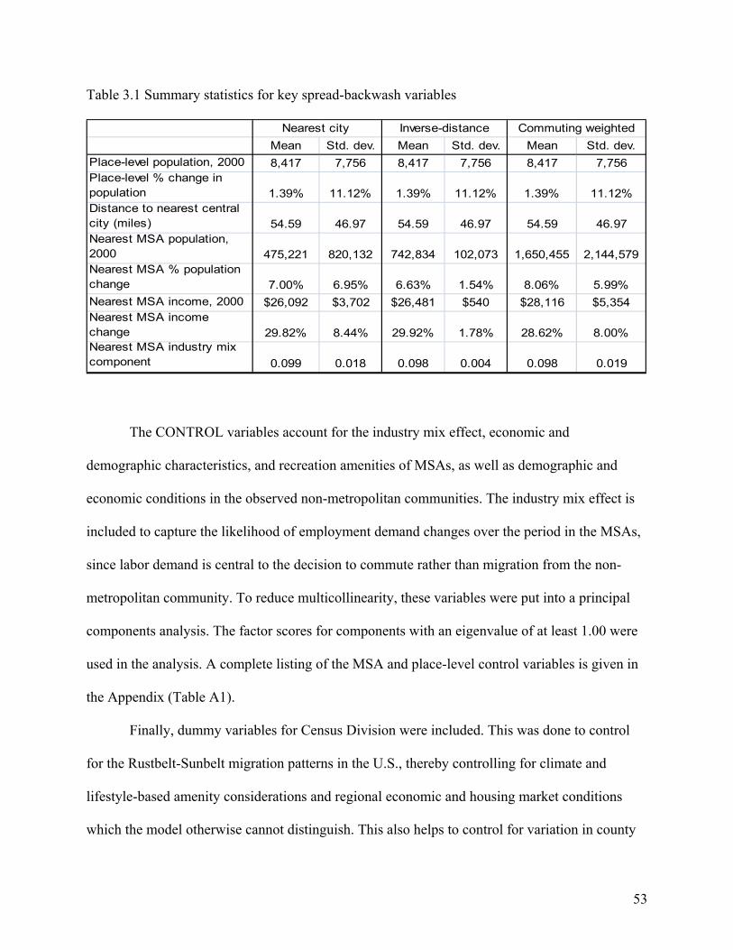
53
Table 3.1 Summary statistics for key spread-backwash variables
Mean Std. dev. Mean Std. dev. Mean Std. dev.
Place-level population, 2000 8,417 7,756 8,417 7,756 8,417 7,756Place-level % change in population 1.39% 11.12% 1.39% 11.12% 1.39% 11.12%Distance to nearest central city (miles) 54.59 46.97 54.59 46.97 54.59 46.97Nearest MSA population, 2000 475,221 820,132 742,834 102,073 1,650,455 2,144,579Nearest MSA % population change 7.00% 6.95% 6.63% 1.54% 8.06% 5.99%
Nearest MSA income, 2000 $26,092 $3,702 $26,481 $540 $28,116 $5,354Nearest MSA income change 29.82% 8.44% 29.92% 1.78% 28.62% 8.00%Nearest MSA industry mix component 0.099 0.018 0.098 0.004 0.098 0.019
Nearest city Inverse-distance Commuting weighted
The CONTROL variables account for the industry mix effect, economic and
demographic characteristics, and recreation amenities of MSAs, as well as demographic and
economic conditions in the observed non-metropolitan communities. The industry mix effect is
included to capture the likelihood of employment demand changes over the period in the MSAs,
since labor demand is central to the decision to commute rather than migration from the non-
metropolitan community. To reduce multicollinearity, these variables were put into a principal
components analysis. The factor scores for components with an eigenvalue of at least 1.00 were
used in the analysis. A complete listing of the MSA and place-level control variables is given in
the Appendix (Table A1).
Finally, dummy variables for Census Division were included. This was done to control
for the Rustbelt-Sunbelt migration patterns in the U.S., thereby controlling for climate and
lifestyle-based amenity considerations and regional economic and housing market conditions
which the model otherwise cannot distinguish. This also helps to control for variation in county
54
size across the U.S.; counties in the American West are much larger than those east of the
Mississippi River. Consequently, it is likely that some Western non-metropolitan places are
farther from central cities than are eastern non-metropolitan places. This effect should be
captured by the inclusion of the DIVISION term.
In general, the models are specified as given below, (equation 2).
G i(t-0)= α + θPOPDENi0 + ψSPATIALi0 + β1X1 + β2X2+ β3X3+ β4X4 + γDIVISIONi0 + εi(t-0)
(2)
Where Gi = percent population change in community i.
X1…4 terms represent the components (constructed from the CONTROL variables)
defined in the principal components analysis. The number of components varies between
the three sets of models; the nearest city models have seven components, the inverse-
distance models have five, and the commuting weighted models have four. The
specification in (3) illustrates the functional form in generalities.
For the first conceptual measurement, in which only the characteristics of the nearest MSA are
considered, the specification in (2) is straightforward. In the second (inverse-distance weighted)
and third (commuting-weighted) models, the specification is markedly different and novel.
In the second and third models, the SPATIAL variables that describe the nearest MSA
(population change in the nearest MSA, income change in the nearest MSA, etc.) are constructed
by multiplying row-standardized weights matrices by a matrix of the MSA-level SPATIAL
variables. In the case of the inverse-distance weighted approach, a row-standardized weights
matrix of the inverse distance between each non-metropolitan place and MSA is used. This is
constructed by taking the matrix of inverse distance between each non-metropolitan place and
55
each MSA (where non-metropolitan places are on the x-axis and MSAs are on the y-axis),
summing each row, then dividing each cell in the row by the row’s total, such that the inverse
distances between each non-metropolitan place and each MSA sums to one for each non-
metropolitan place. This row-standardized matrix is then multiplied against the explanatory
variables. In the case of the commuting-weighted model, a row-standardized matrix of the
normalized commute flow between non-metropolitan place and MSA is used.
Conceptually, row standardizing means that all non-metropolitan places have equal
(distance-based) access to cities and equal (full) commuting access to cities. Using these weights
results in a constructed composite city, where proximate/commuting-linked cities are given
weight according to their proximity or strength of commuting tie. The row-standardized weights
were also used to create a composite “nearest” city for the MSA-level control variables. The
row-standardized weights are also used to calculate the MSA-level CONTROL variables for
each observation.
The distance-interacted SPATIAL terms are constructed similarly, except that the
weights matrices are not row-standardized. This allows non-metropolitan places with stronger
commuting relationships or closer distances to cities to have a larger urban influence than places
with weaker ties. Rather than using distance to the nearest MSA, these models approximate the
interaction of distance to the composite city with the SPATIAL variables.
In sum, nine models are presented in the results. For each of the three approaches (nearest
city, inverse-distance, and commuting weighted), the full model was arrived at in three stages,
the first including only SPATIAL variables, the second adding the CONTROL variables, and the
third adding the DIVISION variables. All nine models shown initially had heteroskedastic errors,
56
which I addressed using a White correction. The final specification is followed by a description
of each term and its variables.
Population change was also measured for 2000-2006 (in addition to 2000-2007) to test
the robustness of the model and its sensitivity over time. The right hand side variables use 2000
data, as described. The sample size is 276 MSAs and 2,170 non-metropolitan communities
(incorporated Census places3). Non-metropolitan communities include those places that are not
in central or outlying metropolitan counties using the 1999 Office of Management and Budget
(OMB) definition for MSAs. The sample is restricted to Census Designated Places that are
incorporated or are minor civil divisions in selected states. Many of the MSAs changed
boundaries between 2000 and 2007. Places that were non-metropolitan in 2000 and metropolitan
in 2007 were not excluded from the sample. Excluding these places would prevent the
observation of the places that are gaining dramatic spread effects via commuting. A
comprehensive list of the variables with data sources is provided in the Appendix (Table A1).
3.4 Results and Discussion
The results for the period 2000-2007 are shown below in Tables 3.2-3.4. These results are
strongly similar to the results for population change from 2000-2006, which was included as a
test of robustness of the model. The CONTROL variables are omitted from this presentation due
to space constraints. They are generally statistically significant with the anticipated signs.
Significance symbols are standard: * p < 0.10; ** p < 0.05; *** p < 0.01. The full names for the
abbreviated regions are given in the Appendix (Figure A1).
3 Roughly 400 Census Designated Places had to be removed from the sample because population estimates for 2007 were not available. The Census Bureau provides population estimates for all incorporated places and minor civil divisions in selected states; not all Census Designated Places are incorporated.

57
Table 3.2: Nearest city models
coeff.White s.e. Sig. coeff.
White s.e. Sig. coeff.
White s.e. Sig.
Intercept 1.19E+01 4.3713 *** 2.77E+01 4.9652 *** 1.73E+01 4.8733 ***Log of population density -1.81E+00 0.4360 *** -3.43E+00 0.5069 *** -2.97E+00 0.5410 ***Dist to nearest central city -5.63E-02 0.0526 -4.43E-02 0.0558 ** -2.13E-02 0.0534 *
Square of dist to the nearest central city -6.68E-05 0.0000 ** -6.66E-05 0.0000 *** -4.96E-05 0.0000 ***
Access Total * 2.30E+01 7.1261 *** 2.24E+01 6.9304 *** 2.38E+01 6.9052 ***% pop change in the nearest MSA 4.04E-01 0.0710 *** 2.91E-01 0.0744 *** 2.06E-01 0.0718 ***Dist x % pop change in the nearest MSA 3.21E-04 0.0013 -5.37E-04 0.0013 * -6.71E-04 0.0012 *% inc change in the nearest MSA -1.97E-02 0.0459 -8.50E-03 0.0442 ** 2.67E-02 0.0459 *Distance x % inc change in the nearest MSA 1.78E-03 0.0007 ** 8.00E-04 0.0007 ** 1.58E-04 0.0007 **Pop, 2000, in the nearest MSA -1.79E-03 0.0013 -1.30E-03 0.0013 ** -1.19E-03 0.0013 *Dist x pop in the nearest MSA 5.26E-05 0.0000 ** 3.21E-05 0.0000 ** 3.50E-05 0.0000 *Inc in the nearest MSA -8.25E-02 0.1240 -1.92E-01 0.1428 * -1.76E-01 0.1369 *Dist x inc in the nearest MSA 7.64E-05 0.0014 5.61E-04 0.0016 ** 1.71E-04 0.0015 **
ESC 7.59E+00 1.4344 ***
PCF 1.09E+01 1.7121 ***
MNT 1.11E+01 1.5762 ***
WSC 5.60E+00 1.1887 ***
SA 8.98E+00 1.3033 ***
ENC 4.07E+00 1.1265 ***
MA 3.65E+00 1.3015 ***WNC 3.54E+00 1.1266 ***
Adjusted R^2
SPATIAL SPATIAL + CONTROL FULL
0.1424 0.2383 0.272

58
Table 3.3: Inverse-distance weighted models
coeff.White s.e. Sig. coeff.
White s.e. Sig. coeff.
White s.e. Sig.
Intercept -2.92E+01 31.2693 6.91E+01 41.4506 * 5.62E+01 40.5919
Log of popdensity -2.78E+00 0.5344 *** -3.61E+00 0.6037 *** -3.21E+00 0.6039 ***Dist to the nearest central city -3.30E-02 0.0133 ** -2.23E-02 0.0121 * -3.43E-02 0.0126 ***Square of dist to the nearest central city 7.80E-06 0.0000 -6.80E-06 0.0000 5.76E-06 0.0000% pop change in the composite nearest city 5.51E+00 0.8742 *** 4.10E+00 0.9896 *** 1.44E+00 1.3103Distance x % pop change in nearest city -5.12E+00 1.6867 *** -2.79E+00 1.6610 * 6.50E-01 2.4169% inc change in nearest composite city -9.39E-01 0.7384 -9.81E-01 0.7136 2.17E-01 1.0749Dist x % inc change in nearest city 1.27E+00 1.2539 2.41E+00 1.2670 * 1.10E+00 1.7479Pop, 2000, in composite nearest city 7.27E-03 0.0170 1.43E-02 0.0223 2.22E-02 0.0226Dist x pop in nearest city 2.13E-02 0.0308 2.48E-02 0.0360 2.00E-02 0.0380Inc in composite nearest city 1.33E+00 1.2483 -2.38E+00 1.9469 -3.12E+00 1.9510Dist x inc in nearest city -5.68E-01 1.6373 -1.72E+00 1.6316 -1.14E+00 1.8892
ESC 1.08E+01 2.2688 ***
PCF 1.16E+01 3.0271 ***
MNT 1.18E+01 2.5679 ***
WSC 7.85E+00 2.0785 ***
SA 1.12E+01 2.0144 ***
ENC 8.13E+00 1.8862 ***
MA 5.41E+00 1.9483 ***
WNC 6.66E+00 2.0687 ***
Adjusted R 2̂
SPATIAL SPATIAL + CONTROL FULL
0.1582 0.2327 0.2486
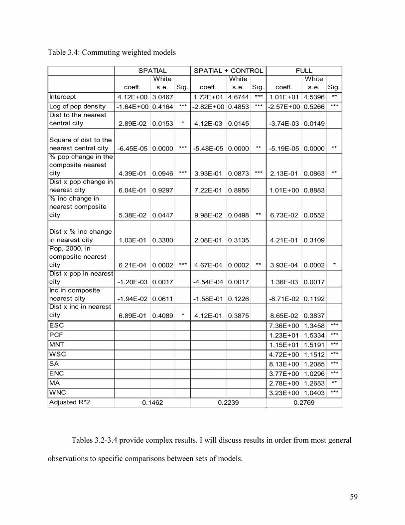
59
Table 3.4: Commuting weighted models
coeff.White s.e. Sig. coeff.
White s.e. Sig. coeff.
White s.e. Sig.
Intercept 4.12E+00 3.0467 1.72E+01 4.6744 *** 1.01E+01 4.5396 **
Log of pop density -1.64E+00 0.4164 *** -2.82E+00 0.4853 *** -2.57E+00 0.5266 ***Dist to the nearest central city 2.89E-02 0.0153 * 4.12E-03 0.0145 -3.74E-03 0.0149
Square of dist to the nearest central city -6.45E-05 0.0000 *** -5.48E-05 0.0000 ** -5.19E-05 0.0000 **% pop change in the composite nearest city 4.39E-01 0.0946 *** 3.93E-01 0.0873 *** 2.13E-01 0.0863 **Dist x pop change in nearest city 6.04E-01 0.9297 7.22E-01 0.8956 1.01E+00 0.8883% inc change in nearest composite city 5.38E-02 0.0447 9.98E-02 0.0498 ** 6.73E-02 0.0552
Dist x % inc change in nearest city 1.03E-01 0.3380 2.08E-01 0.3135 4.21E-01 0.3109Pop, 2000, in composite nearest city 6.21E-04 0.0002 *** 4.67E-04 0.0002 ** 3.93E-04 0.0002 *Dist x pop in nearest city -1.20E-03 0.0017 -4.54E-04 0.0017 1.36E-03 0.0017Inc in composite nearest city -1.94E-02 0.0611 -1.58E-01 0.1226 -8.71E-02 0.1192Dist x inc in nearest city 6.89E-01 0.4089 * 4.12E-01 0.3875 8.65E-02 0.3837
ESC 7.36E+00 1.3458 ***
PCF 1.23E+01 1.5334 ***
MNT 1.15E+01 1.5191 ***
WSC 4.72E+00 1.1512 ***
SA 8.13E+00 1.2085 ***
ENC 3.77E+00 1.0296 ***
MA 2.78E+00 1.2653 **
WNC 3.23E+00 1.0403 ***
Adjusted R^2
SPATIAL SPATIAL + CONTROL FULL
0.1462 0.2239 0.2769
Tables 3.2-3.4 provide complex results. I will discuss results in order from most general
observations to specific comparisons between sets of models.
60
An evaluation of each table quickly indicates that the commuting-based model fails the
preliminary test of external reliability; the sign on distance is positive. The rejection of this
model clearly indicates that market effects are more important in producing spread effects than is
commuting alone. On this point, the term “Access Total” in the nearest city model is simply the
percent of each non-metropolitan place’s commuters that work in MSAs. The consistent
statistical significance of this term indicates that commuting access is a critical element in
delivering spread effects. However, considering a place’s exposure to a city only through the lens
of its commuters produces unreliable results for the measurement of spread and backwash
effects.
In comparing the remaining two sets of models, the nearest city models and the inverse-
distance models, the nearest city models appear stronger. Variable signs are consistent from
model to model, the adjusted R-squared terms are higher, and the variables are generally
statistically significant. That the nearest city model is stronger indicates that while it remains
likely that non-metropolitan places experience spread and backwash effects from multiple
MSAs, a more selective weighting scheme might be appropriate. Such a weighting scheme might
rely on a combination of commuting and freight shipments from places to MSAs. Going back to
the example of grain shipments through the Midwest, farmers in Southern Illinois do not ship
grain equally to every city within a three hundred mile radius, but rather focus shipments to
places where brokers work. Data indicating production volumes for goods in places and purchase
volumes for goods in MSAs could drastically enhance the measurement of spread-backwash
effects.
I will focus now on more specific statistics in Table 3.2, the nearest city model. The pure
distance effect, or UDD, itself is interesting. It is clear that urban proximity produces spread
61
effects for non-metropolitan places. After taking into account the terms for distance to the
nearest city and its square, as well as the interaction terms (distance * x), I calculated that only at
405 miles from a central city does the growth benefit of urban proximity diminish to zero. This
means that all but about half a dozen places in the sample benefit from urban proximity. This
finding is consistent with regional science theory; within the United States (or any country), no
local economy is truly closed. The assumption of a closed economy is a simplification. With an
open economy, no observable place is truly outside the realm of urban spread and backwash
effects.
Larger populations in nearby MSAs also produce spread effects for non-metropolitan
places, theoretically by acting through congestion to discourage in-migration or by driving a
spatial widening of economic activity for the region. The full model in Table 3.2 reinforces not
only that larger populations produce spread effects, but that higher incomes attract people away
from outlying areas and into the city, producing backwash effects. These conflicting spread and
backwash effects were anticipated based on the existing literature. I had also hypothesized that
population growth and income growth would have similar effects; population growth in the city
would deter migration out of non-metropolitan places, while income growth would produce
backwash effects for non-metropolitan places. Table 3.2 shows the spread effect of population
growth on non-metropolitan places and shows backwash effects of income growth on only the
first two models. The signs on the interaction terms (distance * income, distance * income
change, distance * population, distance * population change) are also significant but do not show
the anticipated conflicting signs (positive for population and population growth, negative for
income and income growth).
62
The place-level and MSA-level controls are not reported because they are generally
statistically significant and with the expected sign. I have chosen, however, to report the Census
Division dummy variables in Tables 3.2-3.4 because the results are more interesting. The Census
Division variables are all consistently both positive and statistically significant in all nine models
presented (New England is the reference category). In the nearest city model, the coefficients
vary from 3.54 in the West North Central region to 11.08 in the Mountain Region. This partially
captures the Frost Belt-Sun Belt migration patterns in the U.S.
3.5 Conclusion
This paper sought to quantify spread and backwash effects of MSAs on population
growth in non-metropolitan communities in the U.S. and compare results generated through three
approaches. I find that the traditional nearest city model provides the most reliable results. This
indicates that non-metropolitan places develop their local economies around the demands of the
proximate market, rather than participating in more global markets. The results indicate that
while commuting plays a major role in delivering spread effects into non-metropolitan areas, it is
access to a focused market that is more significant. The results also show that while access to
multiple MSAs may benefit a non-metropolitan place, more detailed information on economic
linkages between places and cities is necessary to develop a more appropriately weighted model.
The results of this model show the anticipated sign on distance, which has the clearest
theoretical antecedents. This approach shows spread effects from population growth and
backwash effects from income change in the nearest city, which is consistent with previous
research. In the nearest city and other approaches, the MSA and place-level control variables are
generally significant and with the expected signs. The addition of Census Division dummy

63
variables strengthens the models and shows the well-known Frost Belt-Sun Belt migration
patterns typical in the U.S.
In sum, this paper compares results of a spread-backwash model using three different
approaches to conceptual measurement. Based on empirical findings, the nearest city model
appears to be the most ideal specification, though potential advancements remain. One potential
advancement is a model that could distinguish between the spread and backwash effects that act
through commuting and those permitted by the flow of goods. A better approximation of the
level of infrastructure that permits commuter and goods flows would also enhance future
research in this area.
64
3.6 Bibliography
Ali, Kamar, M. Rose Olfert, and Mark D. Partridge. 2010. Urban footprints in rural Canada:
Employment spillovers by city size. Regional Studies.
Artís, Manuel, Javier Romaní, and Jordi Suriñach. 2000. Determinants of individual commuting
in Catalonia, 1986–91: Theory and empirical evidence. Urban Studies 37(8): 1431-1450.
Aschauer, David Alan. 1989. Is public expenditure productive? Journal of Monetary Economics
23: 177-200.
Berry, Brian J. L. 1970. Labor market participation and regional potential. Growth & Change
1(4): 3-10.
Boarnet, Marlon G. 1994. An empirical model of intrametropolitan population and employment
growth. Papers in Regional Science 73(2): 135-152.
Bureau of Economic Analysis. 2000, 2007. REIS Table CA1-3, “Per capita personal income.”
Carlino, Gerald A., and Edwin S. Mills. 1987. The determinants of county growth. Journal of
Regional Science 27(1): 39-54.
Chandra, Amitabh, and Eric Thompson. 2000. Does public investment affect economic activity?
Evidence from the rural interstate highway system. Regional Science and Urban Economics
30: 457-490.
Eliasson, Kent, Urban Lindgren, and Olle Westerlund. 2003. Geographical labour mobility:
Migration or commuting? Regional Studies 37(8): 827.
Florida, Richard. 2002. The rise of the creative class. New York: Basic Books.
Gaile, G. L. 1980. The spread-backwash concept. Regional Studies 14(1): 15-25.
Ganning, Joanna and Courtney Flint. In press. Constructing a community-level amenity index.
Society and Natural Resources.

65
Garcia-Milà, Teresa, and Therese J. McGuire. 1992. The contribution of publicly provided inputs
to states' economies. Regional Science and Urban Economics 22(2): 229-241.
Gessaman, Paul, and Daniel Sisler. 1976. Highways, changing land use, and impacts on rural
life. Growth & Change (April 1976): 3-8.
Graves, Philip E. 1980. Migration and climate. Journal of Regional Science 20(2): 227-237.
Greene, William H. 1997. Econometric Analysis (3rd ed.). Upper Saddle River, NJ: Prentice Hall.
Hansen, Niles, Benjamin Higgins, and Donald J. Savoie. 1990. “Regional economic
development policies and programs in the United States: A critical overview and
implications for the future.” Chapter 5 in Regional policy in a changing world. New York:
Plenum Press.
Henry, Mark S., David L. Barkley, and Shuming Bao. 1997. The hinterland's stake in
metropolitan growth: Evidence from selected southern regions. Journal of Regional Science
37(3): 479.
Henry, Mark, Bertrand Schmitt, Knud Kristensen, David Barkley, and Shuming Bao. 1999.
Extending Carlino-Mills models to examine urban size and growth impacts on proximate
rural areas. Growth and Change 30(Fall 1999): 526-548.
Henry, Mark, Bertrand Schmitt, and Virginie Piguie. 2001. Spatial econometric models for
simultaneous systems: Application to rural community growth in France. International
Regional Science Review 24(2): 171-193.
Hirschman, Albert O. 1959. “Interregional and international transmission of economic growth.”
Chapter 10 in The strategy of economic development. New Haven: Yale University Press.
Little, Jo, and Patricia Austin. 1996. Women and the rural idyll. Journal of Regional Studies 12:
101-111.

66
Moss, Joan, Claire Jack, and Michael Wallace. 2004. Employment location and associated
commuting patterns for individuals in disadvantaged rural areas in Northern Ireland.
Regional Studies 38(2): 121-136.
Myrdal, Gunnar. 1957. “The drift towards regional economic inequalities in a country.” In
Economic theory and under-developed regions. London: Gerald Duckworth.
Partridge, Mark D., Ray D. Bollman, Rose Olfert, and Alessandro Alasia. 2007. Riding the wave
of urban growth in the countryside: Spread, backwash, or stagnation? Land Economics
83(2): 128-152.
Partridge, Mark D. and Dan S. Rickman. 2003. Do we know economic development when we
see it? Review of Regional Studies 33(1): 17-39.
Rappaport, Jordan. 2004a. “Moving to nice weather.” RWP 03-07. Kansas City: Research
Division, Federal Research Bank of Kansas City.
Rappaport, Jordan. 2004b. Why are population flows so persistent? Journal of Urban Economics
56(3): 554-580.
Rephann, Terance, and Andrew Isserman. 1994. New highways as economic development tools:
An evaluation using quasi-experimental matching methods. Regional Science and Urban
Economics 24: 723-751.
Rey, S.J. and Marlon Boarnet. 1998. A taxonomy of spatial econometric models for systems of
simultaneous equations. In Anselin, L. and RJGM Florax (eds) Advances in spatial
econometrics. Springer: Berlin.
U.S. Bureau of the Census. 2000. Census 2000. Washington, D.C.
U.S. Bureau of the Census. 2007. American Community Survey. Washington, D.C.

67
U.S. Department of Transportation, Bureau of Transportation Statistics. Census Transportation
Planning Package 2000. Washington, D.C.
van der Laan, Lambert. 1998. Changing urban systems: An empirical analysis at two spatial
levels. Regional Studies 32(3): 235-247.

68
Chapter 4: Detecting and Specifying Spatial Heterogeneity in Commuting Patterns
4.1 Introduction
At its most basic, suburbanization can be thought of as an increasing population density
at increasing distances from a city center. This process is synonymous with the conversion of
rural land to suburban or urban space, and with a spatial widening of the distribution of the labor
force, if not of productive activity and employment. Describing the process of suburbanization in
greater or more local detail, however, becomes more complex. The variables involved in
individual households’ decisions are diverse, ranging from family situation, accessibility to jobs,
preference for urban and rural amenities, housing preference, and willingness to pay for such
preferences in the form of prices or reduced wages. Furthermore, the spatial form of any given
city, as well as its positioning relative to other cities, influences the relative attractiveness of
residential locations.
Measuring spatial accessibility to jobs is one method of estimating the relative
attractiveness of residential locations within regions. In this perspective, the most desirable
residential locations are those from which residents have access to multiple areas of concentrated
employment opportunities. In these areas, the likelihood of finding a job is higher, changing jobs
is expected to be easier, search costs are lower, and finding jobs for both workers of dual-income
households might be simpler. However, excess commuting will continue for at least two reasons.
First, high accessibility of jobs in the residential area deters migration in favor of commuting
(Elliason, Lindgren, and Westerlund, 2003). In other words, workers are resistant to abandoning
a residential location where the anticipated job search cost is low, even if it means commuting in
the short-run. Second, the ease of changing residential location varies based on the size and

69
vacancy rates of the residential areas (Rouwendal, 1998). For instance, it is much easier to
change residential locations in a town with average vacancy rates (such that households can both
sell their current home and find a suitable new home) than in a place like New York City, where
the search for housing is notoriously difficult. In this illustration, someone who works in New
York City may commute some significant distance to work when there are people who live much
closer to his place of work, simply because the search cost of moving is high. In this perspective,
workers will reside in areas with high accessibility to jobs, but excess commuting will continue.
Other methods of estimating or predicting the relative attractiveness of residential
locations within regions come through more explicit attention to processes of suburbanization
and exurbanization. The competing theories of deconcentration and restructuring debate whether
suburbanization occurs as a shift in preferences regarding residential location and amenities
combined with a diminishing cost of commuting (deconcentration), or in the outward movement
of firms to capture lower operating costs (restructuring). Empirical studies generally favor
deconcentration (see Fuguitt and Beale, 1996; Renkow and Hoover, 2000; see also Frey, 1993
for dissenting findings); both sides are considered in the literature review given below. In the
deconcentration perspective, workers will reside in locations with suburban or rural amenities,
from which commuting is possible.
Empirical work investigating deconcentration and restructuring tends to be non-spatial,
assuming that entire regions are either deconcentrating or restructuring as a whole, and that the
same mechanism of population change explains the shifting spatial structure relationship across
the entire region. Yet there is plenty of theoretical and empirical work, as reviewed below, to
support the hypothesis that regional spatial structure is being built and is changing unevenly
across space at any given time. Some work on investigating residuals from migration models (a
70
popular approach to estimating deconcentration and restructuring) across space has been done
(Fotheringham et al., 2000), and Khan et al. (2001) incorporate local amenities in a model of
population and wage growth given economic growth in nearby counties. However, empirical
work has not been done to investigate the significant variation in deconcentration and
restructuring across space, construct a model specification that reflects that spatial variation, and
tie its results to theory.
Geographically weighted regression (GWR) provides a means to understanding the
nature of the relationship between variables across space (Fotheringham, Charlton, and
Brunsdon, 1998). In this paper, I argue that GWR provides a unique function to the study of
deconcentration and restructuring: it lets researchers disentangle the spatial extent of different
mechanisms of commuting across a region. Unlike testing the residuals of OLS regression for
spatial patterning, GWR allows me to evaluate the spatial patterning in the coefficients of each
independent variable. It allows me to articulate sub-regions where particular mechanisms of
residential turnover are prevalent.
By casual observation (as described in further detail below), it appears that during the
1990s the Chicago region experienced dramatic population change at its fringe. The outlying
metropolitan counties were the fastest-growing segment of the region, and there is strong
evidence of substantial migration across the urban hierarchy represented in the handful of cities
near Chicago. This paper seeks to investigate the mechanisms driving this change across the
collar counties between 1990 and 2000.
Modeling deconcentration and restructuring across space at the urban-rural interface will
provide information relevant to rural development policy, sustainable development, and
infrastructure planning. In rural development policy, the infrastructure developments that allow

71
deconcentration is the same infrastructure that allows spread effects via commuting from non-
metropolitan places (e.g. Berry, 1970; Gessaman and Sisler, 1976; Moss, Jack, and Wallace,
2004; Partridge et al., 2007). Identifying the spatial variation in deconcentration and
restructuring across a region will allow economic development policy to tailor regionally-
focused policies for the rural areas that have substantial linkages to the metropolitan core and
community-specific programs in places where spread effects are unlikely to occur (Henry,
Barkely, and Bao, 1997). Relative to sustainable development, understanding the spatial
variation of deconcentration and restructuring will aid in the development of urban growth
management policies by identifying places that are most likely to experience rapid growth and
the mechanisms that drive that growth.
The remainder of this paper follows in seven sections. The next section gives the
analytical framework. This section sets up the theoretical framework for the measurement of
deconcentration and restructuring by first reviewing the concepts of complementarity and
substitution. Section three provides background literature and hypotheses of deconcentration and
restructuring, substitution and complementarity, and dynamism in regions, with the central
argument that these terms are extremes along a spectrum of more plausible scenarios. Section
four gives an overview of the study region and the components of its growth between 1990 and
2000. In short, it is a complex region, with thirteen MSAs, four states, and outlying metropolitan
counties growing faster than other areas of the region. Section five gives the form of the
econometric analysis, with a review of Geographically Weighted Regression (GWR, used as an
exploratory technique). Section six describes the data used and the transformations done to that
data to optimize both measurement and model performance. Section seven presents the results of
the GWR and the OLS model re-specified using the GWR output. Overall, the model shows

72
clear spatial heterogeneity in the mechanism of deconcentration over space. In the study region,
there is a gradient across which households can choose different combinations of residential
characteristics on which they maximize their household utility. The final section concludes the
paper.
4.2 Analytical Framework
This section sets up a commuting framework based on the rationality of maximizing the
net utility an individual captures by combining work and residence location decisions. Using
Renkow and Hoover (2000) as a starting point, I assume that household utility is given by
( , ( , )U U X H L (1)
Where X is consumption of a composite good, H is consumption of housing services, and L
denotes leisure, including the appeal or place stickiness of having family ties to an area.
Following again Renkow and Hoover (2000), this utility function is subject to a budget
constraint equating household earnings to household expenditures, including the cost of
commuting.
The study of deconcentration and restructuring directly addresses this chapter’s concern
with understanding the mechanisms of explosive population change at Chicago’s fringe. The
most relevant set of hypotheses deals with the movement of people and firms outward from the
nexus of a region. As briefly described in the introduction, the principle theories are
deconcentration and restructuring. Deconcentration theory posits that with decreasing
transportation costs, people can afford to act on the preference for more land, and so choose to
commute to work. In restructuring, industry faces changing economic constraints and

73
opportunities that provide a motive to increase distance from the central city; workers follow
(Audirac and Fitzgerald, 2003; Clark and Kuijpers-Linde, 1994; Renkow and Hoover, 2000).
4.3 Background
This section provides an overview of the literature on the theories of deconcentration and
restructuring, substitution and complementarity (a popular method of measuring deconcentration
and restructuring), and the dynamism inherent in changing regional spatial structure, which
complicates the discrete notions of deconcentration, restructuring, substitution, and
complementarity. A consideration of this literature supports the hypothesis that deconcentration
and restructuring cannot be conceived of without a consideration of space.
Deconcentration and Restructuring
Though the texts cited in the introduction (Fuguitt and Beale, 1996; Renkow and Hoover,
2000; Frey, 1993) are the most closely aligned with the subject matter of this paper, there is a
much broader collection of literature around deconcentration and restructuring. An excellent
review is provided by Audirac and Fitzgerald (2003) which, though it focuses on the role of
information technology, provides a more than sufficient coverage of the terminology. This
review draws heavily on the sources identified there, including direct quotations to introduce
each term.
As Audirac and Fitzgerald introduce it, “In the deconcentration group…we find works in
the human ecology tradition of urban sociology and microeconomic neoclassical approaches in
location decision theories” (2003, p. 482). This theory is fairly straightforward: technology and
infrastructure reduce the cost of travel and communication, allowing households to move to the

74
periphery of a region (Audirac and Fitzgerald, 2003). At the periphery, larger lots and homes are
available, with the full range of bucolic amenities which are attractive for families (Rouwendal
and Meijer, 2001). Brian Berry (1973) was among the earliest scholars to discuss
deconcentration. He posited its development on the compression of time (see also Fishman,
1990) and space, as permitted by technology, and the mobility of social classes, which would
lead to increased education attainment and mobility. One final point worth mentioning is that at
its root, deconcentration is a function of atomistic decision making about trade-offs between
commuting, lifestyle amenities, and access to employment. This is in contrast to the restructuring
school.
The restructuring school, on the other hand, “has its intellectual roots in Marxist political
economy and regulation theories” (Audirac and Fitzgerald, 2003, p. 483). These authors go on to
explain, “Since theories in this school are vastly heterogeneous, it can simply be said that they
emphasize economic and spatial restructuring resulting from (1) technological change, which is
the result of, and the transformational force affecting, the (capitalist) mode of production, and (2)
the role of the state in shaping the conditions for economic growth (capital accumulation)” (p.
483). One of the more consistent themes in the restructuring literature is the transformation of the
urban hierarchy from one based on global ports to one based on global centers of command and
control with the spatial dispersion of standardized or “less intellectual” (Storper, 1997) activities
and back-office functions (Audirac and Fitzgerald, 2003; Sassen, 1994; Sassen, 2002; Scott,
1988; Dunford and Kafkalas, 1992; Coffey and Bailly, 1992). Unlike the deconcentration
literature, restructuring studies “reflect the regulation regimes and the interests of corporate and
public-sector actors” (Audirac and Fitzgerald, 2003, p. 484).

75
Complementarity and Substitution
A popular conceptual measurement for deconcentration and restructuring is the
relationship between in-migration and out-commuting within a jurisdiction (usually the county).
A positive relationship between in-migration and out-commuting is called “complementarity;”
the inverse is “substitution” (Evers, 1989; Renkow and Hoover, 2000). Conceptually, if
households are moving into counties and continuing to work elsewhere (complementarity),
deconcentration is occurring; the cost of commuting has been outweighed by the lifestyle
amenities offered at the periphery. If households are moving into counties to replace commuting
to those counties (substitution), then households are following the spatial movement of corporate
decisions. Complementarity and substitution are conceptual measurements for the theoretical
constructs of deconcentration and restructuring. The logic behind this approach is
straightforward; within limits, it will measure the extent to which households move to take
advantage of amenities at the urban fringe versus move to eliminate a commute. For a detailed
discussion of this approach see Renkow and Hoover (2000) and Evers (1989).
Dynamism
Constructing typologies is an academic exercise that enables the analysis of empirical
data but simultaneously mutes heterogeneity. In reality, deconcentration and restructuring and
complementarity and substitution happen simultaneously within regions; as discrete concepts
they are the polar ends of a spectrum of more plausible scenarios. There is both theoretical and
empirical evidence of this.
Theoretically, there are many hybrid perspectives. Deconcentration and restructuring can
be seen as simultaneous results of the interaction of information technology and development
76
(Amirahmadi and Wallace, 1995). Deconcentration suggests that workers move to the suburbs to
take advantage of lifestyle amenities (e.g., Hirschorn, 2000). Restructuring argues that
corporations move to make their businesses more profitable. A hybrid theory suggests that while
the New Economy urges the reorganization of corporate structure, some firms choose to move to
the periphery for the lifestyle amenities (Beyers, 2000), which is a distinctly atomistic approach
to corporate decision-making (see also Henton and Walesh, 1998).
There is also a theoretical expectation that restructuring and deconcentration would be
spatially heterogeneous. On the deconcentration side, spatial variation in lifestyle amenities
provides an avenue for jurisdictions to compete for knowledge workers (Castells, 1996; Florida,
2000; Henton and Walesh, 1998; Hirschorn, 2000). On the restructuring side, the variation in the
provision of information technology capacity, airports, and other transportation infrastructure
make some peripheral locations more attractive than others as corporate locations (Kasarda,
2000; Occelli, 2000; Feitelson and Salomon, 2000; Rodrigue, 1999). Spatial variation in lifestyle
amenities and infrastructure provision are only two examples of the many potential forces that
theoretically enable deconcentration and restructuring to happen with spatial heterogeneity.
Empirically, to some extent, there is evidence of all of these concepts: deconcentration
(e.g. Renkow and Hoover, 2000) and restructuring (e.g. Frey, 1993); clear spatial heterogeneity
in the relationship between migration and commuting within regions (Clark and Kuijpers-Linde,
1994); and the presence of both complementarity and substitution within a region, though the
evidence for substitution is not statistically significant (Renkow and Hoover, 2000).
It is worth discussing the spatial heterogeneity in the migration-commuting relationship,
as it is central to this paper. In their work comparing commuting within Southern California and
the Randstad, Netherlands, Clark and Kuijpers-Linde (1994) describe Southern California as
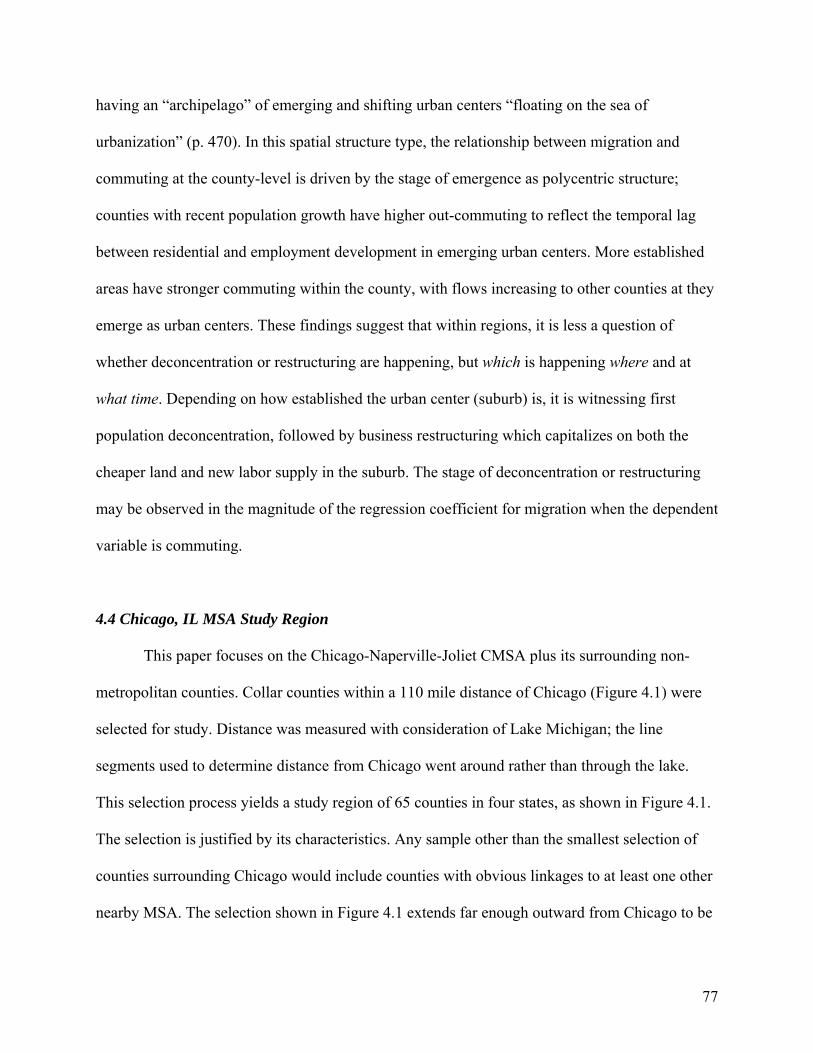
77
having an “archipelago” of emerging and shifting urban centers “floating on the sea of
urbanization” (p. 470). In this spatial structure type, the relationship between migration and
commuting at the county-level is driven by the stage of emergence as polycentric structure;
counties with recent population growth have higher out-commuting to reflect the temporal lag
between residential and employment development in emerging urban centers. More established
areas have stronger commuting within the county, with flows increasing to other counties at they
emerge as urban centers. These findings suggest that within regions, it is less a question of
whether deconcentration or restructuring are happening, but which is happening where and at
what time. Depending on how established the urban center (suburb) is, it is witnessing first
population deconcentration, followed by business restructuring which capitalizes on both the
cheaper land and new labor supply in the suburb. The stage of deconcentration or restructuring
may be observed in the magnitude of the regression coefficient for migration when the dependent
variable is commuting.
4.4 Chicago, IL MSA Study Region
This paper focuses on the Chicago-Naperville-Joliet CMSA plus its surrounding non-
metropolitan counties. Collar counties within a 110 mile distance of Chicago (Figure 4.1) were
selected for study. Distance was measured with consideration of Lake Michigan; the line
segments used to determine distance from Chicago went around rather than through the lake.
This selection process yields a study region of 65 counties in four states, as shown in Figure 4.1.
The selection is justified by its characteristics. Any sample other than the smallest selection of
counties surrounding Chicago would include counties with obvious linkages to at least one other
nearby MSA. The selection shown in Figure 4.1 extends far enough outward from Chicago to be
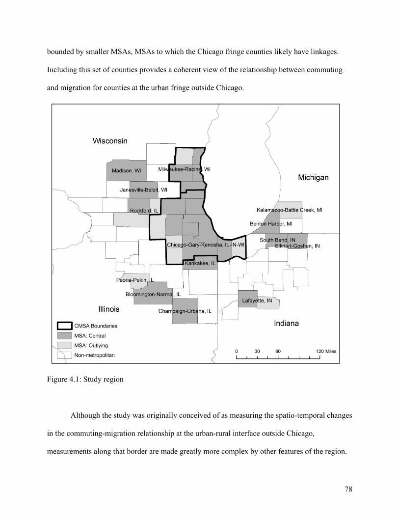
78
bounded by smaller MSAs, MSAs to which the Chicago fringe counties likely have linkages.
Including this set of counties provides a coherent view of the relationship between commuting
and migration for counties at the urban fringe outside Chicago.
Figure 4.1: Study region
Although the study was originally conceived of as measuring the spatio-temporal changes
in the commuting-migration relationship at the urban-rural interface outside Chicago,
measurements along that border are made greatly more complex by other features of the region.
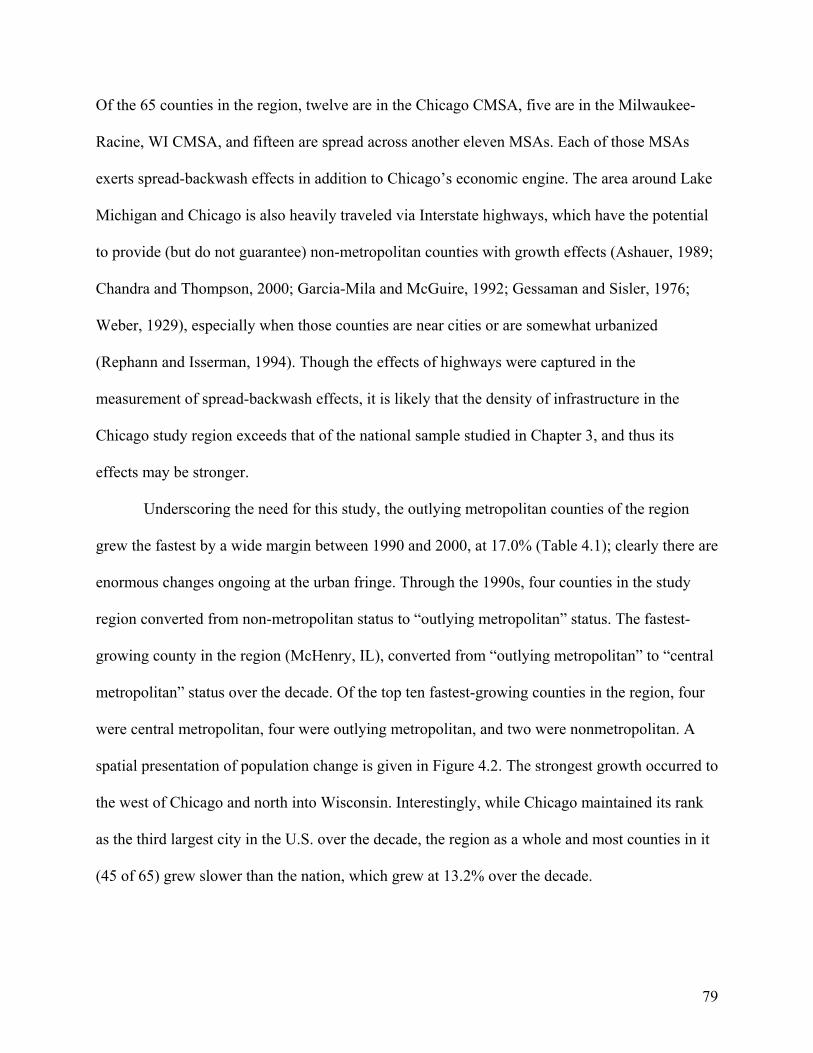
79
Of the 65 counties in the region, twelve are in the Chicago CMSA, five are in the Milwaukee-
Racine, WI CMSA, and fifteen are spread across another eleven MSAs. Each of those MSAs
exerts spread-backwash effects in addition to Chicago’s economic engine. The area around Lake
Michigan and Chicago is also heavily traveled via Interstate highways, which have the potential
to provide (but do not guarantee) non-metropolitan counties with growth effects (Ashauer, 1989;
Chandra and Thompson, 2000; Garcia-Mila and McGuire, 1992; Gessaman and Sisler, 1976;
Weber, 1929), especially when those counties are near cities or are somewhat urbanized
(Rephann and Isserman, 1994). Though the effects of highways were captured in the
measurement of spread-backwash effects, it is likely that the density of infrastructure in the
Chicago study region exceeds that of the national sample studied in Chapter 3, and thus its
effects may be stronger.
Underscoring the need for this study, the outlying metropolitan counties of the region
grew the fastest by a wide margin between 1990 and 2000, at 17.0% (Table 4.1); clearly there are
enormous changes ongoing at the urban fringe. Through the 1990s, four counties in the study
region converted from non-metropolitan status to “outlying metropolitan” status. The fastest-
growing county in the region (McHenry, IL), converted from “outlying metropolitan” to “central
metropolitan” status over the decade. Of the top ten fastest-growing counties in the region, four
were central metropolitan, four were outlying metropolitan, and two were nonmetropolitan. A
spatial presentation of population change is given in Figure 4.2. The strongest growth occurred to
the west of Chicago and north into Wisconsin. Interestingly, while Chicago maintained its rank
as the third largest city in the U.S. over the decade, the region as a whole and most counties in it
(45 of 65) grew slower than the nation, which grew at 13.2% over the decade.
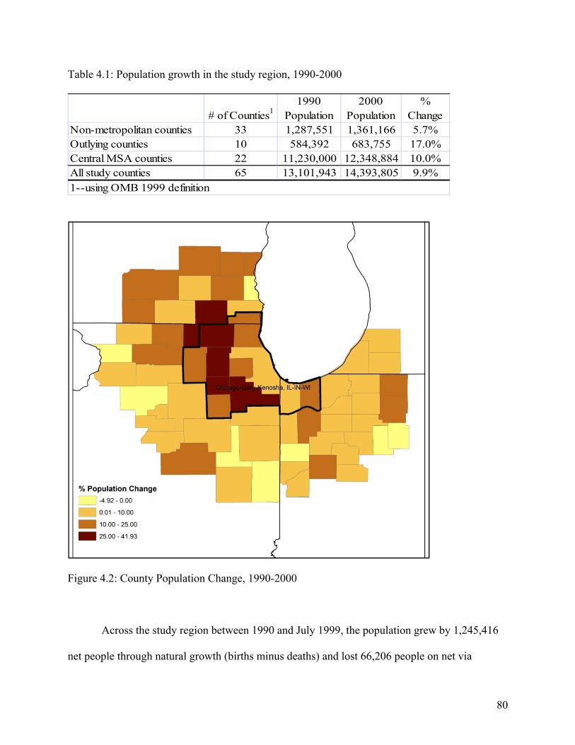
80
Table 4.1: Population growth in the study region, 1990-2000
# of Counties11990
Population2000
Population%
ChangeNon-metropolitan counties 33 1,287,551 1,361,166 5.7%Outlying counties 10 584,392 683,755 17.0%Central MSA counties 22 11,230,000 12,348,884 10.0%All study counties 65 13,101,943 14,393,805 9.9%1--using OMB 1999 definition
Figure 4.2: County Population Change, 1990-2000
Across the study region between 1990 and July 1999, the population grew by 1,245,416
net people through natural growth (births minus deaths) and lost 66,206 people on net via

81
migration. The region lost upwards of half a million people (net of -500,824) via domestic
migration and gained (on net) 434,618 through international migration. Though these sources of
change and their magnitudes seem surprising, in fact they are not unusual for mega-cities
(populations over 2,500,000; Plane, Henrie, and Perry, 2005). In mega-cities, the net migration
rate is positive only in the age bracket 25-29 years (Plane, Henrie, and Perry, 2005). It is
therefore unsurprising that the Chicago CMSA median age is 33.9, or 1.4 years younger than the
national median of 35.3. Migration characteristics, in general, have features specific to
individuals and households in various stages of the life cycle. One key feature pertinent to the
study region is that of household formation and childbearing, both of which encourage growth by
natural causes and migration down the urban hierarchy (Plane, Henrie, and Perry, 2005).
Evidence of this movement can perhaps be seen in the fact that households moving in the 1990s
into Chicago were smaller and earn less than households moving out of the Chicago MSA (Yu,
2009). Stereotypically, young individuals or couples were moving to the city, started building
careers and families, then out-migrating with higher incomes and larger households than when
they arrived. Consequently, the roles of migration and commuting at the urban-rural interface,
and at the interface of a mega-city and nearby smaller cities, become increasingly important.
In 1990, there were 6,167,932 workers who both lived and worked in the study region. Of
those, 1,223,491 (19.8%) commuted across county lines within the study region. In 2000, those
numbers expanded to 6,663,231 workers who both lived and worked in the study region. Of
those, 1,558,551 (23.4%), which constitutes 17.4% of all region residents ages 18-64, commuted
across county lines within the study region. That the percentage of workers commuting over
county lines increased by 27.4% suggests that the spatial distribution of economic activity
expanded during that time. It is more convincing when combined with the fact that four counties
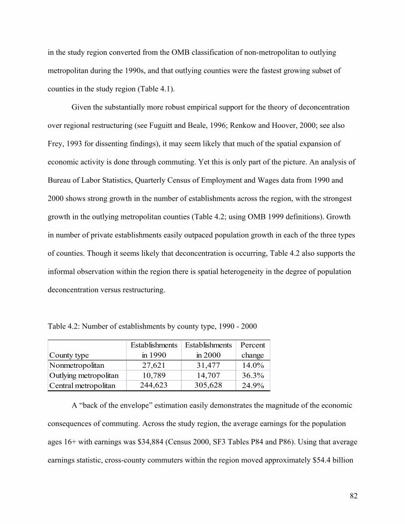
82
in the study region converted from the OMB classification of non-metropolitan to outlying
metropolitan during the 1990s, and that outlying counties were the fastest growing subset of
counties in the study region (Table 4.1).
Given the substantially more robust empirical support for the theory of deconcentration
over regional restructuring (see Fuguitt and Beale, 1996; Renkow and Hoover, 2000; see also
Frey, 1993 for dissenting findings), it may seem likely that much of the spatial expansion of
economic activity is done through commuting. Yet this is only part of the picture. An analysis of
Bureau of Labor Statistics, Quarterly Census of Employment and Wages data from 1990 and
2000 shows strong growth in the number of establishments across the region, with the strongest
growth in the outlying metropolitan counties (Table 4.2; using OMB 1999 definitions). Growth
in number of private establishments easily outpaced population growth in each of the three types
of counties. Though it seems likely that deconcentration is occurring, Table 4.2 also supports the
informal observation within the region there is spatial heterogeneity in the degree of population
deconcentration versus restructuring.
Table 4.2: Number of establishments by county type, 1990 - 2000
County typeEstablishments
in 1990Establishments
in 2000Percent change
Nonmetropolitan 27,621 31,477 14.0%Outlying metropolitan 10,789 14,707 36.3%Central metropolitan 244,623 305,628 24.9%
A “back of the envelope” estimation easily demonstrates the magnitude of the economic
consequences of commuting. Across the study region, the average earnings for the population
ages 16+ with earnings was $34,884 (Census 2000, SF3 Tables P84 and P86). Using that average
earnings statistic, cross-county commuters within the region moved approximately $54.4 billion

83
through the region in 2000. It is critical for municipalities to better understand the drivers of
commuting to better capture a piece of that $54.4 billion practice.
This study region offers several benefits. Though the inclusion of a second CMSA and
eleven other MSAs in the study region complicates analysis, it also provides a rich context. For
example, the complex region allows me to test hypotheses of the attractiveness of access to
multiple cities from a residential location (Eliasson, Lindgren, and Westerlund, 2003). The
selection of this region is also based on data availability, and the opportunity to work alongside
students doing related work in the Regional Economics Applications Laboratory at the
University of Illinois at Urbana-Champaign.
4.5 Econometric Analysis
The previous section described migration and commuting for the Chicago, IL MSA
region for 1990 and 2000. This section outlines an econometric specification of those cross-
county commuting trends and reviews the econometric methods used.
Empirical Model Specification
The empirical form specifies the variables believed to contribute to a household’s decision to
commute or migrate when trying to maximize household utility given budget and time
constraints (as given in equation 1). These variables include place-specific housing
considerations, distance (time constraints) measurements between home and work, a measure of
place stickiness (ethnic concentration), and potential to increase wages by commuting. The
empirical form given is
( , , , , , )ji ji jiij i ij iC f W H Q E D M (2)

84
Where
Cij = net number of workers commuting from county i to county j, normalized by the
employed population of county i (this is a departure from Renkow-Hoover)
jiW = wage in county j minus wage in county i
jiH = standardized housing cost in county j minus county i
jiQ = four-year college degree attainment rate in county j minus county i
Ei = concentration of ethnicities in county i
Dij = distance between counties i and j, using population-weighted centroids
Mi = net migration into county i in the previous period, normalized by the population in
county i in the previous period
I normalize net commuting by the employed population of county i. This is done to scale
the value of commuting. The wage, housing, and distance variables are included as significant
push and pull factors in the decision to migrate or commute. A commuter should logically want
to maximize income while minimizing housing costs and distance traveled. I also include a
measure of the difference in educational attainment between counties. This measure is calculated
by taking the percent of the population with at least a bachelor’s degree then subtracting county
j’s score from that of county i. I do this to introduce a control for the skill level available in the
labor market, to control for spatial mismatch of jobs to skills. A measurement of this differential
is particularly necessary in situations where there is significant cross-commuting, for example,
when central city residents work in the suburbs and suburban residents work in the central city.
I include a measure for a key amenity that cannot be assumed to be capitalized in the
housing and wage prices—family ties. This aspect of “place stickiness” is proxied by a Simpson
85
index of ethnic concentration in each county, which measures the probability that “any two
members selected at random from a population will belong to different groups” (Plane and
Rogerson, 1994, p. 302). It is assumed that people like being near other like people, to enjoy
ethnic customs, family bonds, and a sense of commonality in community. This is not an
argument for segregation, but rather for the value of family and the idea that absolute integration
is also unfavorable.
Finally, rather than using the difference in median housing costs between counties, I
calculate a difference in housing costs for comparable units, by using HUD’s Fair Market Rent
statistics. This marks a significant departure from the literature, where traditionally housing
prices have been compared across geographic units at the median, without respect to
characteristics (e.g. McMillen, 2003). Using Fair Market Rents allows me to control for the size
and general quality of the housing unit. This is important considering the key demographic that
moves into and out of mega-cities—young people and new households, respectively. For a new
household, housing units of equal price in a central city and a suburb or smaller city are
absolutely unequal, with unit size being one of several key distinctions. A hedonic housing index
would be ideal, but the data is not available at the county level.
On a substantive level, this paper acknowledges that the tools to measure the variation in
the commuting-migration relationship are newer than much of the research in this area, and their
application to this research question is novel. There are questions left unanswered in existing
research; are the statistically insignificant occurrences of negative migration coefficients
indicative of undetected, spatially distinct causal mechanisms in the commuting-migration
relationship? How can research on the relationship between commuting and migration better
inform scholars on the mechanisms of population growth at the urban-rural interface? I address
86
these unanswered questions by first using GWR, which gives a detailed view of the spatial
variation in the relationships between commuting and the independent variables listed above.
Output from the GWR model will be incorporated into a clustering algorithm, which will define
based on the GWR coefficients discrete sub-regions within the study area. I then interact dummy
variables for each region with the independent variables in an OLS model to verify whether the
spatial patterning in the GWR betas is significant in modeling commuting across the region.
The econometric analysis is carried out in two stages. The first stage uses GWR. The
coefficients of the GWR are used as input in a clustering algorithm which defined sub-regions in
the study area. Dummy variables for the sub-regions are interacted with the variables in the
empirical specification and re-tested via OLS to test the hypothesis that there is statistically
significant spatial variation in the commuting-migration relationship.
Geographically Weighted Regression (GWR)
GWR is a technique used “to examine the spatial variability of regression results across a
region and so inform on the presence of spatial nonstationarity” (Fotheringham, Charlton, and
Brunsdon, 1998). Its general form, GWR can be expressed as:
0 ( , )k i i ikiy a a u v x (3)
Where u and v are coordinates of the ith point, allowing a continuous surface of parameter values
(Fotheringham, Charlton, and Brunsdon, 1998, p. 1907). This technique produces localized
regression diagnostics. To allow calibration of the model, points nearer to point i are given more
weight in the estimation of the parameter value for point i,
â(ui,vi) = [XTW(ui,vi)X]-1XT W·(ui,vi)y (4)

87
One technical consideration of this approach is that it is meant to model values at i.
However, the dependent variable used in this paper is the commuting flow between ij pairs of
counties, meaning there are multiple data points for each sending county i. A hierarchical
approach may be more ideal. However, the GWR is used in this paper to delineate sub-regions
on which to test the spatial heterogeneity of the mechanism of deconcentration. It is not used to
draw conclusions. The statistical significance of sub-regions in the final specification is
sufficient evidence that the GWR has functioned satisfactorily for the purpose of this research.
McMillen (2004) briefly reviews the GWR concept and different perspectives on its use.
From a conceptual perspective, there are two characteristics that distinguish GWR from other
parametric and nonparametric approaches. Unlike nonparametric approaches, GWR does not
focus on nonlinearity in independent variables, but rather is appropriate for situations of linearity
between the dependent and independent variables at a given location. Second, and perhaps its
hallmark, GWR estimates the spatial variation in the coefficient for each variable. This is
especially helpful when it is unclear whether: (1) different socioeconomic, demographic, or
related situations cause different commuting mechanisms, which could be detected by finding
spatial patterning in the average x values or by spatial patterning in the (average) βx values by
county i (where observations are ij pairs of counties), or; (2) the model is either misspecified or
underestimating the value of place.
This latter point deserves attention. In his review McMillen (2004) provides a clear
articulation of the principal difference between applied geographers and applied economists. The
former, he says, see spatial variation in regression coefficients as “consistent with post-modernist
beliefs on the importance of place and locality as frames of understanding…behavior” (a direct
quote from Fotheringham, Charlton, and Brunsdon, 2002). Applied economists, on the other
88
hand, believe GWR helps to detect model misspecification; they dismiss out of hand that the
price of a standard good (his example is a garage) truly varies over space, but rather can be
modeled based on its qualities and the qualities of nearby amenities. As he writes, “GWR is a
useful regression diagnostic; we have more faith in our specification if the results are not altered
by the use of GWR. If the results change, it is an indication that more investigation is in order,
not that the price of a garage is truly different in different parts of a city” (2004, p. 556).
In the case of modeling commuting in a large, city-focused region, I argue that there is
growing room for both arguments. There is a literature speculating that households choose
residential locations for the intangible character of the place (Castells, 1996), and similarly that
firms develop organizational structures that respond to local contexts (Belussi, 2000). However,
it is also true that the growing literature on and tools to measure place-based amenities is
growing (e.g., Ganning and Flint, forthcoming). This paper takes the first of two steps that are
critical in fully developing our understanding of mechanisms of commuting and thus of
population growth mechanisms at the urban-rural interface: (1) detecting the presence of and
geographic extent of “local contexts” which influence commuting within a region and (2) more
fully investigating those contextual elements. The latter may be better suited to survey-based
research, qualitative inquiry, or case study research, which is beyond the scope of this paper.
4.6 Data
This paper relies primarily on three databases: the Census of Population and Housing
(2000), the Census Transportation Planning Package (CTPP 2000), and migration data from the
Internal Revenue Service (IRS, 1990-2000). Though the Census databases provide information
for a finer level of geography, the IRS files are available only at the county level. Additionally,

89
in CTPP data there is a trade-off between spatial resolution and data disclosure, making difficult
an analysis where each place of residence and place of employment pair are assessed separately.
Therefore, the county is the unit of observation for this study. The full range of regression
variables by data source used is given in Table 4.3. Additionally, population at the block group
and county levels for 2000 was used to establish population-weighted centroids for each county.
Table 4.3: Variables for Geographically Weighted Regression
Variable Definition Source Cij Net commuting from county i
to county j, standardized by the employed population of county i
CTPP 2000
Wij Difference in wages between county i and county j.
Bureau of Economic Analysis, 2000
Hij Difference in the Fair Market Rent of a 2-bedroom apartment between county i and county j
HUD Fair Market Rent
Qij Difference in four-year college degree attainment rates between county i and county j
Census 2000
Ei Concentration of ethnicities in county I, measured using a Simpson index4
Census 2000 (SF3, Table PCT 18)
Dij Distance between counties i and j, with distance measured from the block group population-weighted centroid of each county
Census 2000, and ArcMap 9.3
Mi Net migration into county i in the previous year, normalized by population in the previous year
IRS county-to-county migration tables, 1998-1999
4 S = 1 - 2
1
( / )n
k
k
P P

90
The wage data represents wages at the place of employment rather than the place of
residence. This figure is the relevant one in modeling commuting rates since people commute to
earn a wage that is offered somewhere other than the home county. Optimizing household utility
is a combination of residential and work location choices, the latter of which is based largely on
wage and availability of employment suitable to one’s skill set. College education attainment
includes all people ages 25+ living in a place who have earned a four-year degree or higher;
those with some college or associates degrees are not counted as having attained a four year
degree.
The difference in housing costs is controlled for by comparing the Fair Market Rent of
two-bedroom apartments using data from the Department of Housing and Urban Development
(HUD). Comparing housing costs in county-level research has long plagued researchers. Data
that provides enough information to construct true hedonic housing price indices are generally
not available at the county level.5 The HUD data has the distinct advantage of comparing
equivalent housing units across space. The HUD data is also favorable for its continuity, though
this paper does not take advantage of that feature; it is available for every year between 1983 and
2009, with changes in calculation methods clearly identified.
I began by limiting the data set to the ij county pairs that had non-zero net commuting,
and from those selected only the observations with positive net commuting, as is established in
the literature to avoid selection bias (Renkow and Hoover, 2000). I then limited the data set again
to include only ij pairs that are neighbors in a second order (first order inclusive) queen weights
matrix. The weights used to determine those pairings was developed in GeoDa. Invoking a
5 Such information is publicly available for PUMAs, which sometimes correspond to counties, but often encompass several counties, making analysis difficult. Information regarding house size, sales price, and other characteristics can sometimes be obtained from housing authorities or local Realtor associations. In those cases, that data is preferable to the rental cost information used here.

91
spatial limit also helps to eliminate observations with commute flows so small as to be within a
reasonable margin of error. Finally, the model uses the log of net commuting as its dependent
variable. This transformation was necessary to meet the assumption that the relationships
between the dependent and independent variables be linear. After limiting the data to positive net
commute observations within 2 neighboring counties, the data set includes 388 ij pairs in 2000.
The analysis was carried out using R. I used the function gwr.sel (spgwr) in R to select the
bandwidth, which is 0.8638697 decimal degrees.
4.7 Results
Geographically Weighted Regression
It should be said that improving on the existing OLS model of commuting flows will be
difficult. Not only do Renkow and Hoover (2000) report reasonable strength in their OLS
models, but the straight OLS model of commuting near Chicago is quite strong (Table 4.4).
These results are shown with White-corrected standard errors (White, 1980; R code for White
correction by Gianfranco Piras and provided by Professor Kathy Baylis). The model did not
show multicollinearity. The variables that are common between this and the Renkow and Hoover
(2000) approach show the same signs, giving a measure of external validity.
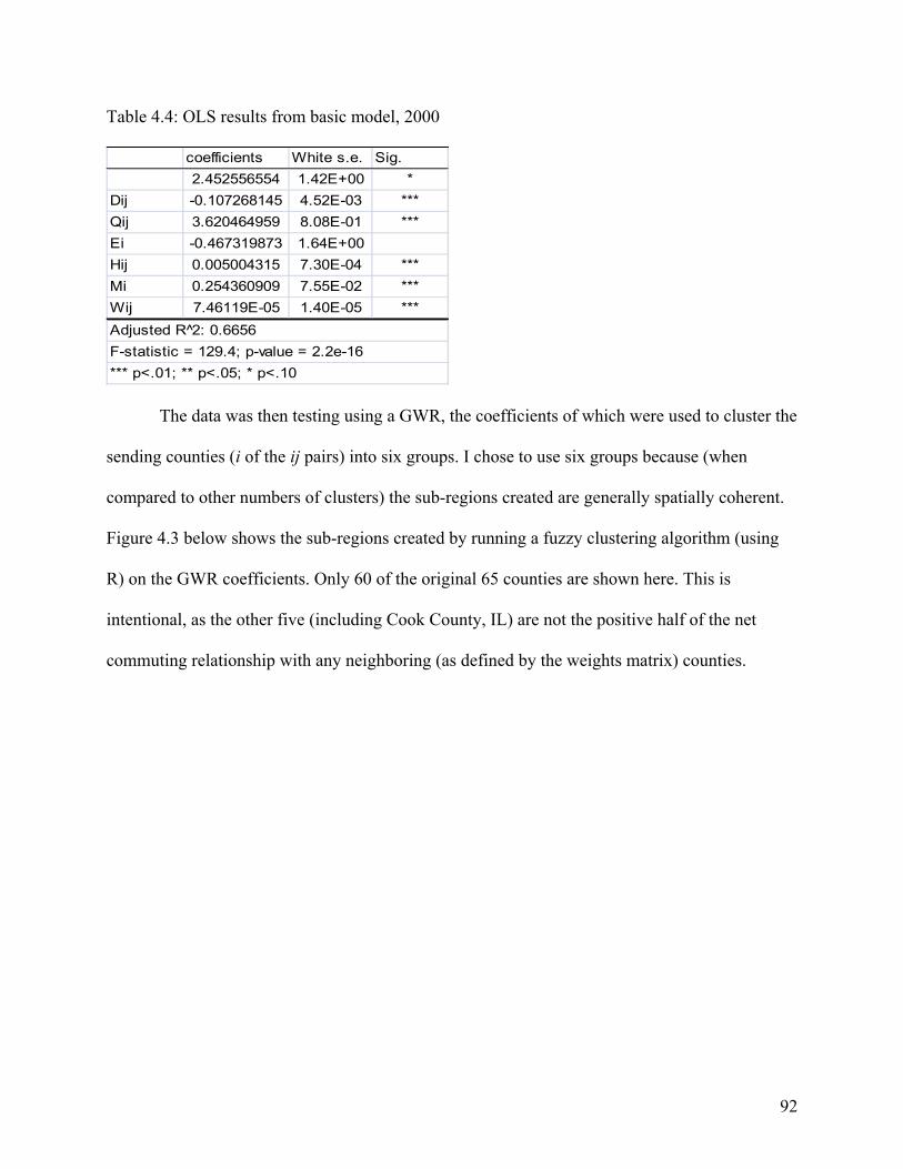
92
Table 4.4: OLS results from basic model, 2000
coefficients White s.e. Sig.
2.452556554 1.42E+00 *
Dij -0.107268145 4.52E-03 ***
Qij 3.620464959 8.08E-01 ***
Ei -0.467319873 1.64E+00
Hij 0.005004315 7.30E-04 ***
Mi 0.254360909 7.55E-02 ***
Wij 7.46119E-05 1.40E-05 ***
*** p<.01; ** p<.05; * p<.10
Adjusted R 2̂: 0.6656
F-statistic = 129.4; p-value = 2.2e-16
The data was then testing using a GWR, the coefficients of which were used to cluster the
sending counties (i of the ij pairs) into six groups. I chose to use six groups because (when
compared to other numbers of clusters) the sub-regions created are generally spatially coherent.
Figure 4.3 below shows the sub-regions created by running a fuzzy clustering algorithm (using
R) on the GWR coefficients. Only 60 of the original 65 counties are shown here. This is
intentional, as the other five (including Cook County, IL) are not the positive half of the net
commuting relationship with any neighboring (as defined by the weights matrix) counties.
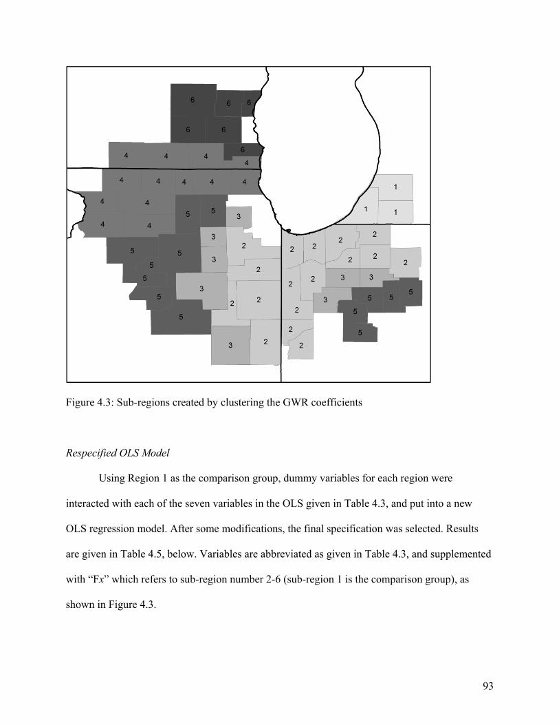
93
Figure 4.3: Sub-regions created by clustering the GWR coefficients
Respecified OLS Model
Using Region 1 as the comparison group, dummy variables for each region were
interacted with each of the seven variables in the OLS given in Table 4.3, and put into a new
OLS regression model. After some modifications, the final specification was selected. Results
are given in Table 4.5, below. Variables are abbreviated as given in Table 4.3, and supplemented
with “Fx” which refers to sub-region number 2-6 (sub-region 1 is the comparison group), as
shown in Figure 4.3.
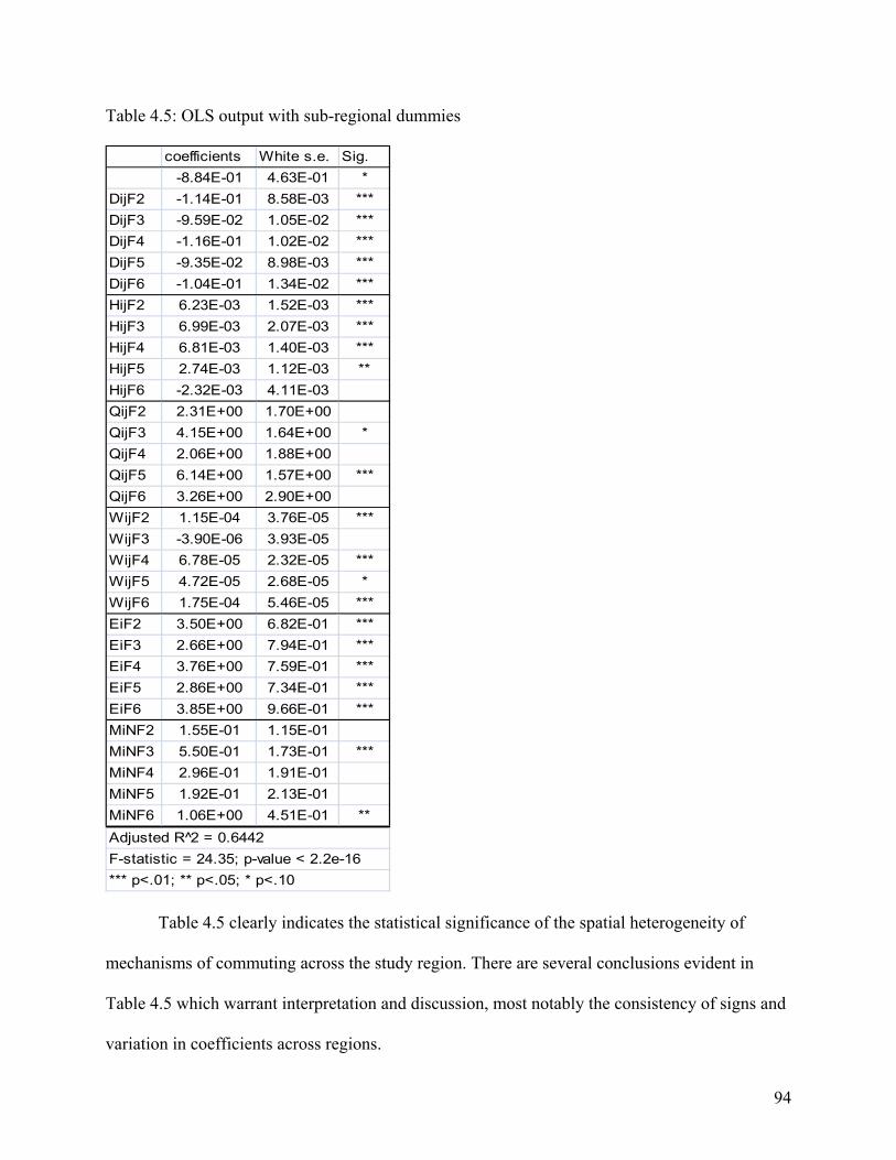
94
Table 4.5: OLS output with sub-regional dummies
coefficients White s.e. Sig.
-8.84E-01 4.63E-01 *
DijF2 -1.14E-01 8.58E-03 ***
DijF3 -9.59E-02 1.05E-02 ***
DijF4 -1.16E-01 1.02E-02 ***
DijF5 -9.35E-02 8.98E-03 ***
DijF6 -1.04E-01 1.34E-02 ***
HijF2 6.23E-03 1.52E-03 ***
HijF3 6.99E-03 2.07E-03 ***
HijF4 6.81E-03 1.40E-03 ***
HijF5 2.74E-03 1.12E-03 **
HijF6 -2.32E-03 4.11E-03
QijF2 2.31E+00 1.70E+00
QijF3 4.15E+00 1.64E+00 *
QijF4 2.06E+00 1.88E+00
QijF5 6.14E+00 1.57E+00 ***
QijF6 3.26E+00 2.90E+00
WijF2 1.15E-04 3.76E-05 ***
WijF3 -3.90E-06 3.93E-05
WijF4 6.78E-05 2.32E-05 ***
WijF5 4.72E-05 2.68E-05 *
WijF6 1.75E-04 5.46E-05 ***
EiF2 3.50E+00 6.82E-01 ***
EiF3 2.66E+00 7.94E-01 ***
EiF4 3.76E+00 7.59E-01 ***
EiF5 2.86E+00 7.34E-01 ***
EiF6 3.85E+00 9.66E-01 ***
MiNF2 1.55E-01 1.15E-01
MiNF3 5.50E-01 1.73E-01 ***
MiNF4 2.96E-01 1.91E-01
MiNF5 1.92E-01 2.13E-01
MiNF6 1.06E+00 4.51E-01 **
*** p<.01; ** p<.05; * p<.10
Adjusted R 2̂ = 0.6442
F-statistic = 24.35; p-value < 2.2e-16
Table 4.5 clearly indicates the statistical significance of the spatial heterogeneity of
mechanisms of commuting across the study region. There are several conclusions evident in
Table 4.5 which warrant interpretation and discussion, most notably the consistency of signs and
variation in coefficients across regions.
95
The consistency of signs for any given variable across the five regions (where sub-region
1 was the reference region) was unexpected and lends significant credibility to the hypothesis
that even diverse regions tend to deconcentrate and/or suburbanize as regions, even if the extent
of that deconcentration is uneven across space. In both Renkow and Hoover (2000) and in early
exploratory work for this manuscript, a statistically insignificant but negative sign on in-
migration was found for some types of counties in some years. This suggested that breaking the
region down into sub-regions might reveal pockets where the mechanism of commuting is
drastically different, yet this has proven not to be the case. All of the signs are consistent and in
the hypothesized direction in Table 4.5. It is interesting, however, that the sign on ethnicity (Ei)
changed between the standard OLS and the respecified OLS given in Table 4.5, and the variable
became statistically significant. This signals that simpler models that pool counties into one large
region or distinguish them based on the discrete notions of “urban” and “rural” are muting the
significance of this variable across space. Breaking a region into sub-regions paints a more
complete picture of the gradient in commuting mechanisms across space.
As expected, the sign on the migration term is positive. Unexpectedly, the migration term
is statistically significant for only two of the five sub-regions (Table 4.5). The coefficients of
those two sub-regions, however, are telling. In sub-region 3 the coefficient on migration is
double its value for sub-region 6. This indicates that while both sub-regions are undergoing
population deconcentration, that process is much more pronounced in the Illinois outskirt of
Chicago than in the northern outskirt of Milwaukee.
It is important to ask if the results shown in Table 4.5 so clearly indicate the significance
of spatial heterogeneity in mechanisms of commuting across space because the x-bar values
vary, because the coefficients vary, or due to an average effect. Using the county-level output
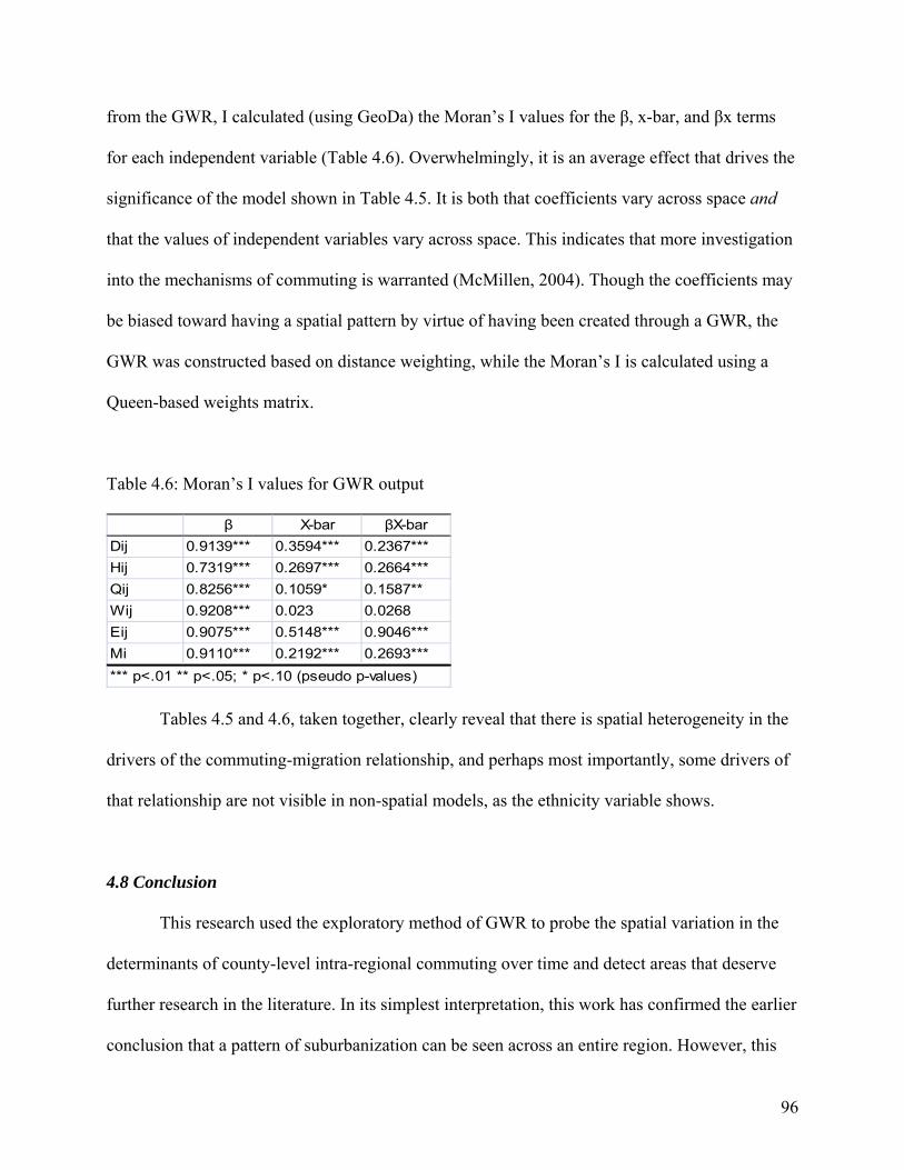
96
from the GWR, I calculated (using GeoDa) the Moran’s I values for the β, x-bar, and βx terms
for each independent variable (Table 4.6). Overwhelmingly, it is an average effect that drives the
significance of the model shown in Table 4.5. It is both that coefficients vary across space and
that the values of independent variables vary across space. This indicates that more investigation
into the mechanisms of commuting is warranted (McMillen, 2004). Though the coefficients may
be biased toward having a spatial pattern by virtue of having been created through a GWR, the
GWR was constructed based on distance weighting, while the Moran’s I is calculated using a
Queen-based weights matrix.
Table 4.6: Moran’s I values for GWR output
β X-bar βX-bar
Dij 0.9139*** 0.3594*** 0.2367***
Hij 0.7319*** 0.2697*** 0.2664***
Qij 0.8256*** 0.1059* 0.1587**
Wij 0.9208*** 0.023 0.0268
Eij 0.9075*** 0.5148*** 0.9046***
Mi 0.9110*** 0.2192*** 0.2693***
*** p<.01 ** p<.05; * p<.10 (pseudo p-values)
Tables 4.5 and 4.6, taken together, clearly reveal that there is spatial heterogeneity in the
drivers of the commuting-migration relationship, and perhaps most importantly, some drivers of
that relationship are not visible in non-spatial models, as the ethnicity variable shows.
4.8 Conclusion
This research used the exploratory method of GWR to probe the spatial variation in the
determinants of county-level intra-regional commuting over time and detect areas that deserve
further research in the literature. In its simplest interpretation, this work has confirmed the earlier
conclusion that a pattern of suburbanization can be seen across an entire region. However, this
97
work adds nuance to that finding by applying a statistical technique which post-dates the bulk of
research on this topic. This work indicates that the degree of suburbanization varies across a
region and that there is spatial patterning in the regression coefficients, signaling the need for
more in-depth understanding of commuting mechanisms.
These results point to the need for increased research in the areas of residential amenity
measurement for urban regions, as well as to the different but potentially equal (given variation
in households’ calculations of utility) pecuniary benefits of living in the urban core. This work
could be approached through hedonic housing analysis (if adequate data were available) or
through survey research, to name a few possibilities. This work must emphasize and draw on the
observation from this work that the notions of “explosive population growth at the urban-rural
fringe” and clean distinctions between deconcentration and restructuring are artificial. The
results clearly indicate a gradient across the region, where tradeoffs between space, accessibility,
and other variables are made. The GWR output does not delineate an urban and a rural, a “young
peoples’ community” or a “dual-income household” community. It shows a gradient across
which households can choose the amenities and features that will maximize their utility in many
combinations of methods.
In conclusion, updated econometric tools now enable the advancement of our
understanding of mechanisms of commuting. There is a regional gradient across which different
features of residential space are given higher and lower premiums, appealing to individuals
wishing to maximize utility individually. Estimating a commuting function based on distance or
crude categorization of counties over-simplifies and obscures drivers of the decision to commute
or migrate. This perspective embraces on one hand a post-modernist perspective that individuals
seek to combine different bundles of goods in unique ways which could include intangible place

98
qualities, and on the other hand embraces the applied econometric perspective that finding
statistically significant coefficients across a region points to a model misspecification. In any
case, the toolbox now available to spatial econometricians demands that we reject what is clearly
an over-simplified depiction of commuting in regions.

99
4.9 Bibliography
Amirahmadi, H., and C. Wallace. 1995. Information technology, the organization of production,
and regional development. Environment and Planning A 27: 1745-1775.
Aschauer, David Alan. 1989. Is public expenditure productive? Journal of Monetary
Economics 23: 177-200.
Audirac, Ivonne, and Jennifer Fitzgerald. 2003. Information technology (IT) and urban form: An
annotated bibliography of the urban deconcentration and economic restructuring
literatures. Journal of Planning Literature 17(4): 480-511.
Belussa, Fiorenza. 2000. Towards the post-Fordist economy: Emerging organizational models.
International Journal of Technology Management 32(1/2): 20-43.
Berry, Brian J. L. 1970. Labor market participation and regional potential. Growth & Change
1(4): 3-10.
------. 1973. The human consequences of urbanization. London: Macmillan.
Beyers, William B. 2000. Cyberspace or human space: Wither cities in the age of
telecommunications? In Cities in the telecommunications age, James O. Wheeler, Yuko
Aoyama, and Barney Warf, eds. New York: Routledge.
Bureau of Economic Analysis. 2000. REIS Table CA34, “Average wage per job.” Washington,
D.C.
Castells, Manuel. 1996. Megacities and the end of urban civilization. New Perspectives
Quarterly 13(3): 12-15.
Chandra, Amitabh, and Eric Thompson. 2000. Does public investment affect economic activity?
Evidence from the rural interstate highway system. Regional Science and Urban
Economics 30: 457-490.
100
Clark, William A. V., and Marianne Kuijpers-Linde. 1994. Commuting in restructuring urban
regions. Urban Studies 31(3): 465-483.
Coffey, William J. and Antoine S. Bailly. 1992. Producer services and systems of flexible
production. Urban Studies 29(6): 857-868.
Department of Housing and Urban Development. 2000. “Fair Market Rents.” Retrieved from
http://www.huduser.org/portal/datasets/fmr.html (August 1, 2009).
Dunford, Michael and Grigoris Kafkalas, eds. 1992. Cities and regions in the new Europe.
London: Belhaven.
Eliasson, Kent, Urban Lindgren, and Olle Westerlund. 2003. Geographical labour mobility:
Migration or commuting? Regional Studies 37(8): 827.
Evers, Gerard. 1989. “Simultaneous models for migration and commuting: Macro and micro
economic approaches.” In Migration and labour market adjustment, p. 177-197. Dordrecht,
Netherlands: Kluwer Academic Publishers.
Feitelson, Eran and Ilan Salomon. 2000. The implications of differential network flexibility for
spatial structures. Transportation Research Part A 34 (2000): 459-479.
Fishman, Robert. 1990. America’s new city: Megalopolis unbound. Wilson Quarterly 14(1): 25-
45.
Florida, Richard. 2000. Competing in the age of talent: Environment, amenities and the new
economy. Report prepared for the R.K. Mellon Foundation, Heinz Endowments, and
Sustainable Pittsburgh.
Fotheringham, A. Stewart, Tony Champion, Colin Wymer, and Mike Coombes. 2000. Measuring
destination attractivity: A migration example. International Journal of Population
Geography 6: 391-421.
101
Fotheringham, A. Stewart, M. E. Charlton, and C. Brunsdon. 1998. Geographically weighted
regression: A natural evolution of the expansion method for spatial data analysis.
Environment & Planning A 30(11): 1905-1927.
Frey, W. H. 1993. The new urban revival in the United States. Urban Studies 30: 741-74.
Fuguitt, Glenn V., and Calvin L. Beale. 1996. Recent trends in nonmetropolitan migration:
Toward a new turnaround? Growth & Change 2(2): 156.
Ganning, Joanna P., and Courtney G. Flint. Forthcoming. Constructing a community-level
amenity index. Society and Natural Resources.
Garcia-Milà, Teresa, and Therese J. McGuire. 1992. The contribution of publicly provided inputs
to states' economies. Regional Science and Urban Economics 22(2): 229-241.
Gessaman, Paul, and Daniel Sisler. 1976. Highways, changing land use, and impacts on rural
life. Growth & Change (April 1976): 3-8.
Gober, Patricia, Kevin E. McHugh, and Denis Leclerc. 1993. Job-rich by housing poor: The
dilemma of a western amenity town. Professional Geographer 45(1): 12-20.
Henry, Mark S., David L. Barkley, and Shuming Bao. 1997. The hinterland's stake in
metropolitan growth: Evidence from selected southern regions. Journal of Regional Science
37(3): 479.
Henton, Doug and Kim Walesh. 1998. Linking the New Economy to the livable community. A
report to the James Irvine Foundation. San Francisco: The James Irvine Foundation.
Hirschorn, Joel S. 2000. Growing pains: Quality of life in the new economy. Washington, DC:
National Governors’ Association. Retrieved from
http://www.nga.org/cda/files/GROWINGPAINS.pdf (December 13, 2009).
Internal Revenue Service. 1999. “County-to-county migration data.” Washington, D.C.
102
Kasarda, John D. 2000. New logistics technologies and infrastructure for the digital economy.
Chapel Hill: Kanan Institute of Private Enterprise, University of North Carolina. Retrieved
from http://in3.dem.ist.utl.pt/downloads/cur2000/papers/S19P01.pdf (December 13, 2009).
Khan, Romana, Peter F. Orazem, and Daniel M. Otto. 2001. Deriving empirical definitions of
spatial labor markets: The roles of competing versus complementary growth. Journal of
Regional Science 41(4): 735.
McMillen, Daniel P. 2003. Employment subcenters and home price appreciation rates in
metropolitan Chicago. In Advances in Econometrics, volume 18, eds. James LeSage, Kelley
Pace.
McMillen, Daniel P. 2004. Review of “Geographically Weighted Regression: The Analysis of
Spatially Varying Relationships,” by A. Stewart Fotheringham, Chris Brunsdon, and Martin
Charlton. American Journal of Agricultural Economics 86(2): 554-556.
Moss, Joan, Claire Jack, and Michael Wallace. 2004. Employment location and associated
commuting patterns for individuals in disadvantaged rural areas in Northern Ireland.
Regional Studies 38(2): 121-136.
Occelli, Sylvie. 2000. “Revisiting the concept of accessibility: Some comments and research
questions.” In Information space and cyberspace, Donald G. Janelle and David C. Hodge,
eds. New York: Springer.
Partridge, Mark D., Ray D. Bollman, Rose Olfert, and Alessandro Alasia. 2007. Riding the wave
of urban growth in the countryside: Spread, backwash, or stagnation? Land Economics
83(2): 128-152.
Pisarski, Alan E. 2006. Commuting in America III. Washington, D.C.: Transportation Research
Board of the National Academies, NCHRP Report 550/TCRP Report 110.
103
Plane, D. A., C. J. Henrie, and M. J. Perry. 2005. Migration up and down the urban hierarchy and
across the life course. Proceedings of the National Academy of Sciences of the United States
of America 102(43): 15313-8.
Plane, David A., and Peter A. Rogerson. 1994. The geographic analysis of population with
applications to planning and business. New York: John Wiley & Sons, Inc.
Renkow, Mitch, and Dale Hoover. 2000. Commuting, migration, and rural-urban population
dynamics. Journal of Regional Science 40(2): 261.
Rephann, Terance, and Andrew Isserman. 1994. New highways as economic development tools:
An evaluation using quasi-experimental matching methods. Regional Science and Urban
Economics 24: 723-751.
Rodrigue, Jean-Paul. 1999. Globalization and the synchronization of transport terminals. Journal
of Transport Geography 7: 255-261.
Rouwendal, Jan. 1998. Search theory, spatial labor markets, and commuting. Journal of Urban
Economics 43(1): 1-22.
Rouwendal, Jan, and Erik Meijer. 2001. Preferences for housing, jobs, and commuting: A mixed
logit analysis. Journal of Regional Science 41(3).
Sassen, Saskia. 2002. Cities in a world economy. In Readings in urban theory, eds. S. Fainstein,
S. Campbell. 2nd ed., 32-56. Malden, MA: Blackwell Publishing.
------. 1994. Cities in a world economy. Thousand Oaks, CA: Pine Forge Press.
Scott, Allen. 1988. Metropolis: From the division of labor to urban form. Berkeley: University
of California Press.
Storper, Michael. 1997. The regional world. New York: Guilford.
U.S. Bureau of the Census. 2000. Census 2000. Washington, D.C.
104
U.S. Department of Transportation, Bureau of Transportation Statistics. Census Transportation
Planning Package 2000. Washington, D.C.
Weber, Alfred. 1929. Theory of the location of industries. Trans. Carl J. Friedrich. Chicago: The
University of Chicago Press.
White, Halbert. 1980. A heteroskedasticity-consistent covariance matrix estimator and a direct
test for heteroskedasticity. Econometrica 48(4): 817-838.
Yu, Chenxi. 2009. Net migration drains $1.6 billion from Illinois economy each year. Urbana,
IL: Regional Economics Applications Laboratory, University of Illinois Urbana-
Champaign.

105
Chapter 5: Conclusion
This chapter will summarize and synthesize the three substantive chapters of this
dissertation. I will begin by summarizing the main conclusions of each and then in section 5.2
will synthesize those findings into a narrative.
5.1 Summary of Chapters
This dissertation focuses on mechanisms of population growth at the urban-rural
interface. The three substantive papers focus on that theme and inform on it from different
perspectives. All three papers use a common sample of 276 MSAs (and CMSAs) from across the
country. The first paper implements a measure of intra-regional spatial structure that had been
developed and tested for use in the Netherlands and tests the validity of the measure by testing it
against a range of hypotheses regarding spatial structure and socioeconomic trends, as given in
the literature. That paper served as background and database-building work for the second and
third papers. The second paper investigates spread and backwash effects (positive and negative
effects of urban proximity, as measured through population change) for the sample of 276 MSAs
on nearly 2,170 non-metropolitan communities (U.S. Census places) between 2000 and 2007.
The third paper studies mechanisms of commuting within an urban-focused region experiencing
rapid population growth at the urban fringe.
In the paper Chapter 2, I found that the van der Laan (1998) measure of spatial structure
found partial but not universal support when tested against existing theories of about spatial
structure and measures of socioeconomic status and demographics within regions. I found that
regional demographics and some contextual characteristics are linked to spatial structure at
statistically significant levels. The VDL measure N1, which measures traditional commuting,
106
found external validity. However, detecting polycentric spatial structure and relating it to theory
proved more complex, revealing gaps in our understanding of both the mechanisms of
polycentricity and the timing of its formation relative to its drivers. Among the more interesting
findings of this chapter is that larger cities tend to have lower shares of commuters going from
suburbs to central cities. This finding supports the hypothesis that the largest MSAs will have
market-driven polycentricity, developing an “urban archipelago” (Clark and Kuipers-Linde,
1994). This suggests that polycentricity is an on-going process, happening in tandem with the
spatial widening of a growing region’s economy.
In the paper “Spread and Backwash Effects for Non-metropolitan Communities in the
U.S.,” I estimated the extent of pure distance effects of urban growth and tested the hypothesis
that non-metropolitan places experience spread and backwash effects from multiple cities. I
discovered that in the United States, a non-metropolitan place is never far enough away from a
city to experience population growth effects gained by further isolation. The idea that after some
distance a place is insulated from backwash effects simply does not play out using this data. I
also revealed that though the ability to commute to a city is an important ingredient in non-
metropolitan population growth, economic linkages to cities, and most importantly to the nearest
city, play a more important role. This indicates that rather than participating in global markets,
non-metropolitan places are used as suppliers of goods for neighboring cities.
In the third paper, “Detecting and Specifying Spatial Heterogeneity in Commuting
Patterns,” I specified a spatial model of commuting within a region and discovered a large
discrepancy between conclusions drawn from non-spatial versus spatial models of commuting.
Most notably, I discovered spatial heterogeneity in both the values of the right hand side
variables and in the coefficients. Also, I found that a measure of ethnic concentrations is not a

107
statistically significant determinant of commuting in a non-spatial model, but becomes
significant in a spatial model (where ethnicities are concentrated, people more often choose to
commute rather than to migrate, presumably to stay close to family). Overall, the fit of a spatial
model is roughly similar to that of the non-spatial model, but the conclusions drawn vary
significantly, and the coefficients estimated for sub-regions within the study area vary at
statistically significant levels. This research has shown that misspecifications in previous models
lead to potentially inaccurate conclusions. The present research suggests that theoretical
distinctions between urban and rural, and the so-called drastic change at the interface, are over-
simplifications of a region that has sub-regions. These sub-regions create a gradient of potential
combinations of characteristics and amenities by that are considered by consumers to maximize
household utility based on their individual tastes. Future work remains to be done around both
the qualitative and quantitative determinants of estimating household utility.
5.2 Synthesis
These three papers raise questions about both existing theory and empirical findings,
suggest hypotheses for further research, and contribute to methodological advancement in the
study of population growth at the urban-rural interface. In this sub-section, I will synthesize the
conclusions of the three papers into one narrative.
This dissertation has supported many hypotheses and previous research findings. Perhaps
most consistently, I have found that the process of spatial expansion of economic activity works
first by the expansion of residential locations, then by enlargement of population in the fringe
county, and finally by growth in job opportunities in that county. All three papers support this
finding. This is consistent with the deconcentration hypothesis, but puts into relief the fact that
108
deconcentration is only an initial stage in the spatial expansion of economic activity. Where
deconcentration is happening, urban spatial structure is changing. From a policy perspective, it is
important to detect early commuting patterns from the budding fringe counties and enhance the
efficiency of those commuter flows, as they are likely to remain stable in pattern but increase in
volume as the residential population of the county expands. As employment opportunities grow,
the transportation focus will have to expand to allow commuting from other residential areas,
fully integrating the county into the urban archipelago.
The new insights and hypotheses gleaned, however, are much more interesting, and there
are several. The single clearest lesson learned from this dissertation is the importance of taking a
regional perspective in planning. Chapter 2 illustrates the incredible mobility of labor between
city and suburbs, and among suburbs. Chapter 3 clearly demonstrates the importance of linkages
between city and countryside. Chapter 4 shows the fallacy in assuming that counties can be
divided into small pools on the basis of single variables such as “urban” and “rural.” Instead,
households maximize utility by choosing a location along a gradient of sub-regions that offer
many different combinations of amenities and features, according to a household’s taste. In all of
these examples, it is the region that grows or declines together. Though central cities historically
played substantial roles as the engines of growth, this research clearly demonstrates the power of
the regional engine instead.
Several implications for policy can be drawn from these conclusions. First, road
construction should focus on connecting suburbs not only to the central city, but also to other
suburbs, and that early commuting patterns emanating from budding residential areas should be
given significant weight in determining future infrastructure needs. Second, if a region has a pro-
growth vision, then planning should facilitate that growth rather than respond to it. Preempting

109
the need for infrastructure as the spatial range of economic activity expands can be facilitated
using concepts advanced in this dissertation.
5.3 Closing
In closing, this dissertation has addressed two mechanisms of population growth at the
urban-rural interface, and among other things detected that even the phrase “urban-rural
interface” may be an over-simplification. This dissertation has paved the way for a tremendous
volume of future work, including work around the process of polycentric evolution, the spatial
extent of economic linkages for non-metropolitan places and the role of ethnic ties in the
decision to commute or migrate within a region, to name a few topics. It has been my hope that
this work would effectively inform rural development theory and policy, and I believe I have
made significant strides in that direction and have established a research agenda around these
themes.

110
Appendix
Figure A1: Census Divisions
Acronyms:
NE: New England
ESC: East South Central
PCF: Pacific
MNT: Mountain
WSC: West South Central
SA: South Atlantic
ENC: East North Central
MA: Middle Atlantic
WNC: West North Central

111
Table A1: Variables in analysis
Variable name Data source Description
Key Variables
Log of population density Census 2000 Using land area only,
population per mile squared
Distance to nearest central
city
Census 2000 TIGER/Line
shapefiles, ArcMap 9.3
Used x, y coordinates to
calculate the Euclidean
distance between each non-
metropolitan place and the
first central city for each
MSA
Access Total Census Transportation
Planning Package, 2000
Percent of non-metropolitan
place commuters who work
in an MSA
MSA-level population and
population change
Census 2000 and Census
Bureau Population
Estimates, 2007
Level variable is divided by
1000
MSA-level income and
income change
Bureau of Economic
Analysis, REIS Tables
Per capita personal income,
2000 and 2007. Level
variable is divided by 1000

112
Place-level controls
Non-white Census 2000 Percent of the population
reporting multiple races or
any non-white race
Elderly Census 2000 Percent of the population
that is age 65 or older
Education attainment Census 2000 Percent of the population
age 25+ that has at least a
bachelors degree
Labor force participation
rate
Census 2000 Percent of the population
age 16+ that is in the labor
force
Unemployment Census 2000 Percent of the population
that is in the labor force and
unemployed
Urban Census 2000 Percent of the population
that is classified as urban
MSA-level controls
Elderly Census 2000 Percent of the population
that is age 65+
Labor force participation
rate
Census 2000 Percent of the population
ages 16+ that is in the labor

113
force
Afford Census 2000 Percent of households
paying less than 35% of
monthly income on selected
housing costs
Non-white Census 2000 Percent of the population
reporting multiple races or
any non-white race
Foreign Census 2000 Percent of the population
that is foreign born
Education attainment Census 2000 Percent of the population
age 25+ that has at least a
bachelors degree
Industry Mix Census 2000, American
Community Survey 2007
Sum of shares of
employment in each
industry multiplied by its
national growth rate from
2000 to 2007. 13 industries
used.
Related Documents