Growth and convergence: A profile of distribution dynamics and mobility

GROWTH AND CONVERGENCE: A PROFILE OF DISTRIBUTION

DYNAMICS AND MOBILITY

ESFANDIAR MAASOUMIDEPARTMENT OF ECONOMICS

SOUTHERN METHODIST UNIVERSITYDALLAS, TX USA 75275-0496

JEFF RACINEDEPARTMENT OF ECONOMICS

SYRACUSE UNIVERSITYSYRACUSE, NY USA 13244-1020

THANASIS STENGOSDEPARTMENT OF ECONOMICS

UNIVERSITY OF GUELPHGUELPH, ONT CAN N1G 2W1

Abstract. In this paper we focus primarily on the dynamic evolution of the world distributionof growth rates in per capita GDP. We propose new concepts and measures of “convergence,”or “divergence” that are based on entropy distances and dominance relations between groups ofcountries over time.

We update the sample period to include the most recent decade of data available, and we offertraditional parametric and new nonparametric estimates of the most widely used growth regressionsfor two important subgroups of countries, OECD and non-OECD. Traditional parametric modelsare rejected by the data, however, using robust nonparametric methods we find strong evidence infavor of “polarization” and “within group” mobility.

Key Words: Growth, convergence, distribution dynamics, entropy, stochastic dominance, non-parametric, international cross-section.

JEL Classification: C13, C21, C22, C23, C33, D30, E13, F43, Q30, Q41.

E. Maasoumi is the corresponding author. His contact information is Department of Economics, Southern MethodistUniversity, Dallas, TX 75275-0496, Email: [email protected], Tel: (214) 768-4298.

1. Introduction

Recent research on growth and convergence has provided a fertile interface between economic

theorists, empirical economists and, increasingly, modern econometricians. It is now more widely

accepted that the research effort in this area should be directed less toward questions of whether

realizations from, or moments of, the distribution of growth rates converge, and more to questions

concerning the “laws” that generate the distribution of growth rates, or incomes, and their evolu-

tion over time. This focus on whole distributions would hide less of the pertinent facts, and is more

conducive to learning the nature and degree of what appears to be an “unconditional” divergence

in growth rates and incomes. There is a well established tradition for our approach in the “income

distribution” literature where ranking of distributions by, for example, Lorenz and Stochastic Dom-

inance criteria, and the study of mobility, are well developed. Quah’s work is rightly associated

with the introduction of the distribution approach in the “growth convergence” literature; see Quah

(1993, 1997).

In this paper we focus on significant features of the probability laws that generate growth rates

that go beyond both the “β-convergence” and “σ-convergence.” It is perhaps necessary to empha-

size how narrow these two concepts are. The former concept refers to the possible equality of a

single coefficient of a variable in the conditional mean of a distribution of growth rates! The latter,

while being derivative of a commonplace notion of “goodness of fit,” also is in reference to the

mere fit of a conditional mean regression, and is additionally rather defunct when facing nonlinear,

nonguassian, or multimodal distributions commonly observed for growth and income distributions.

We will examine the entire distribution of growth rates, as well as the distributions of parametrically

and nonparametrically fitted and residual growth rates relative to a space of popular conditioning

variables in this literature. New concepts of convergence and “conditional convergence” emerge

as we introduce new entropy measures of distance between distributions to statistically examine a

deeper question of convergence or divergence.

Some of our findings may be viewed as alternative quantifications and characterizations of the

distributional dynamics discussed in Quah (1993, 1997). Quah focuses on the distribution of per

capita incomes (and relative incomes) for the same panel of countries in the world. He examines

diffusion processes for the probability law generating these incomes, and a measure of “transition

1

probabilities,” the stochastic kernel, to examine the evolution of the relative per capita incomes.

On the other hand, we examine the distribution of the growth rates themselves, and use entropy

distance metrics that reveal divergences, reflect the nature of divergences, and is closely related

to welfare-theoretic notions of income mobility embodied in the inequality reducing measures of

Shorrocks-Maasoumi-Zandvakili; see Maasoumi (1998).

Our findings are largely based on distributional dynamics and conform more closely with the theo-

retical models which take cross-country interactions into account (such as in Lucas (1993), and Quah

(1997)) or which allow for elements of multiple regimes and certain types of non-convexities (as in

Durlauf and Johnson (1995)). Employing recent techniques for handling mixed discrete/continuous

variables, we also present new nonparametric estimates of both the growth rate distributions (see

Li and Racine (2003, 2004), Racine and Li (2004), and Hall, Racine, and Li (forthcoming)). While

we strongly agree with Quah on the limitations of the traditional panel regression (conditional

mean) analysis in this area, we do connect to, and accommodate the current literature by apply-

ing our nonparametric techniques to the estimation of the most widely analyzed extended form

of the original Solow-Swan regression model (as in Mankiw, Romer and Weil (1992)). But here

too we offer a different (entropy) measure of “fit” for these regressions which may be viewed as

an enhancement of the concept of σ-convergence since it involves many more moments than just

the variance. Making summary statements with conditional means (averages) is not without value,

but our modest message is that one can make better statements and one must caution that some

distributions are poorly summarized by their means and/or variances.

The availability of data on a number of important dimensions that describe domestic economic

activity in a given country and the collection of these individual country data into an international

data source, such as in Summers and Heston (1988) and King and Levine (1993), has allowed a

systematic examination of cross-country growth regressions. Focusing on the conditional means,

the vast majority of the contributions to the empirics of economic growth have assumed that the

main attributes that characterize growth such as physical and human capital exert the same effect

on economic growth both across countries (intratemporally) and across time (intertemporally) and

have assumed a (log) linear relationship (see Barro (1991) and Barro and Sala-i-Martin (1995)).

There have been some recent studies that question the assumption of linearity and propose nonlinear

2

alternatives that allow for multiple regimes of growth patterns among different countries. These

models are consistent with the presence of multiple steady-state equilibria that classify countries

into different groups with different convergence characteristics (see Quah (1996) for a discussion

of the evidence against the convergence hypothesis that underlies the standard approach). In

this context, Bernard and Durlauf (1993) offer an explanation for the apparent strong evidence in

favor of the convergence hypothesis (see Mankiw et al. (1992)). They argue that the convergence

properties for all countries in the misspecified linear model are inherited from the convergence of a

group of countries associated with a common steady state in the correctly specified multiple regime

growth model.

Motivated by recent theories emphasizing threshold externalities (Azariadis and Drazen, (1990)),

Durlauf and Johnson (1995) postulate that countries obey different laws of motion to the steady

state. They employ regression tree methodology and divide countries into four subgroups according

to their initial level of per capita income and literacy rate. They infer distinct linear laws of motion

for the four subgroups. Thus, their work rejects the presumption on which the majority of the

cross-country empirical growth literature is based. In particular, they find substantial differences

in their estimate of the coefficient for the secondary enrollment ratio: it is insignificant for two of

the subsamples and is positive for the other two (it is a third larger in magnitude for the middle

income economies as compared to the high income ones). Hansen (2000) uses a threshold regression

framework to test for sample splitting between different groups of countries and he finds evidence

of such groupings. In a related study using some of the same methods as ours, Liu and Stengos

(1999) allow for two nonlinear components, one for the initial level of GDP and the other for

the secondary enrollment rate. They find that the presence of nonlinearities were mainly due to

groupings of countries according to their level of initial income, whereas the effect of human capital

(as measured by the secondary enrollment rate) was in essence linear.

As has been pointed out by Durlauf and Quah (1999), the dominant focus in these studies is

on certain aspects of estimated conditional means, such as the sign or significance of the coeffi-

cient of initial incomes, how it might change if other conditioning variables are included, or with

other functional forms for the production function or regressions. Many of these empirical models,

including panel data regressions, fail to serve as vehicles to identify and distinguish underlying

3

economic theories with sometimes radically different implications and predictions. Many also run

counter to observed income distributional dynamics, or are unable to explain them. In addition,

all of the above studies rely on “correlation” criteria to assess goodness of fit and to evaluate

“convergence.” Our first step is to rectify this shortcoming, especially when considering nonlinear

and/or nonparametric regressions. This we achieve with two entropy measures of fit. The resulting

analysis produces “fitted values” of growth rates, as well as “residual growth rates” which will be

used for fresh looks at the question of “conditional” convergence. Our nonparametric kernel esti-

mates of conditional growth are free from some of the functional form misspecifications that have

been pointed out by various authors in this area. We shed some light on potential nonlinearities in

growth relations.

Turning to the main objective of this paper, we examine the relation between growth rate distri-

butions for different country groups, as well as the evolution of the generating law over time, both

within and between country groups. The nonparametric density method of Hall et al. (forthcoming)

is utilized to analyze these questions. We quantify these distribution distances and movements by

entropy measures, and use the latter to examine convergence (conditional and unconditional) as a

new statistical hypothesis. Our data are extended beyond previous studies and span the last 35

years of available data.

The plan of the paper is as follows. In Section 2 we present the elements of the traditional

“work horse” model of this literature. In Section 3 we propose to fit parametric and nonparametric

regression models on the data panel for two different groups of countries, the OECD and the “rest

of the world” consisting of the lesser developed countries. We also offer a conditional moment test

of the traditional parametric specification. In Section 4 we present the unconditional distribution

of the growth rates, and the distribution of their fitted values. Next, we obtain k-class entropies of

each distribution, especially for two values of k, the Shannon entropy, and for k=1/2 (see Granger,

Maasoumi and Racine (forthcoming)). Our approach is appealing because the distribution of growth

rates across countries and time cannot be successfully summarized by their variances alone (unless

they are normal). Additionally, inferences regarding the fit of these models is assessed by a metric

entropy measure of distance between the actual and fitted distributions for each country group. We

report the entropy distance between the two groups of countries (both for fitted and actual growth

4

rates). The distance based on “raw” growth rates is a new measure of unconditional convergence.

The one based on the fitted values is a new measure of “conditional convergence.” These entropies

and entropy distances reveal how far apart (dispersed) are the economies within each group and

between the two groups. If indeed there is statistically significant convergence to a common steady

state then one expects that these distance measures “shrink” in size as one moves from the 1960’s

to the 1970’s through the 1990’s. We find that the empirical evidence is compatible with bipolar

development and “clubs.”

Contrary to commonly assumed models, the evolution of these distances or laws may not be

“linear.” For example it may be that the distance first decreases and then increases. Within each

group, even if one finds β-convergence (the coefficient of initial income may be negative, signifying

that a country with a lower GDP will have higher growth rates thereby catching up with the rest

of the countries in the same group), entropy within each group will reveal any unequal pattern of

growth rates (conditional and unconditional). If the growth rates are roughly equal, entropy will

take its maximum value (log N, in the case of Shannon’s, where N is the number of countries in the

group). Thus we are able to reveal more of the growth mobility dynamics even within groups. This

offers an examination of mobility dynamics which tells us how distributions change and by how

much, in the sense of Shorrocks-Maasoumi. In other words we are able to capture nonlinearities

in the growth dynamics of different income classes (heterogeneity in the growth paths). Quah

(1997), looking at the per capita incomes, examines the probabilities of related transitions. This

approach captures the cross-sectional heterogeneity and the tendency towards polarization of the

cross-country distribution.1 The two approaches are clearly interconnected and complementary but

different. Maasoumi (1998) sheds light on the relation between these two notions of mobility.

Our reported entropies in the distributions of growth rates and model residuals for all countries

and both groups reveal why it has been false to assert convergence, in any sense, without grouping

of countries.

What the proposed approach does that has not been done before is to define, measure, and test

for convergence in the probability laws that generate cross-country growth rates, explicitly allow for

1Fiaschi and Lavezzi (2003) have tried to combine the two approaches in a Markov transition matrix framework.However, their approach suffers from the complexity of the state space in terms of both income levels and growthrates, since there is no natural way to obtain its partition ex-ante.

5

heterogeneity between different country groups, and base inferences on more robust nonparametric

estimators.2

2. The Traditional Parametric Setting.

It is helpful to first present the mechanics of the traditional regression models of the conditional

mean of the distribution which will be the primary focus of our work. This regression has been

the main focus in the literature. Our recollection in this section helps to identify some popular

conditioning variables. But we also offer some advances in the analysis of this conditional mean

which would be helpful when one wishes to make statements that are useful “on average” for

sufficiently homogeneous country groups. Mankiw et al. (1992) assume a production function of

the form Yt = Kαt Hβ

t (AtLt)1−α−β , where Y , K, H, and L represent total output, physical capital

stock, human capital stock and labor, respectively, and A is a technological parameter. Technology

is assumed to grow exponentially at the rate φ, or At = A0eφt. By linearizing the transition path

around the steady state, they derive the path of output per effective worker y (y = Y/AL) between

time period T and T + r as follows:

(1) ln yT+r = θ ln y∗ + (1 − θ) ln yT ,

where θ = (1 − e−λr), λ is the rate of convergence and y∗ is the steady state level of output per

effective worker. In order to derive the growth of output per worker (Y/L), they substitute for

the steady state level of output per worker (ln y∗ = α ln k∗ + β ln h∗), noting that the steady state

levels of capital per effective worker (k∗) and human capital per effective worker (h∗) depend on

the share of output devoted to physical capital accumulation (sk), the share of output devoted to

human capital accumulation (sh), the growth of the labor force (n), and the depreciation rate for

(human and physical) capital (δ). Finally, the growth of output per worker between period T and

T + r of country i is obtained by noting that ln yT = ln(Y/L)T − ln A0 −φT and subtracting initial

2Quah (1996, 1997) looks at the distributions of per capita incomes and its various transformations, and theirevolution into a bipolar set. Quah’s work is similar in spirit to ours but does not offer measures of “distance” betweendistributions, as we do.

6

income from both sides of (1) to arrive at:

ln

(Y

L

)

i,T+r

− ln

(Y

L

)

i,T

= φr + θ(ln A0 + φT ) + θα

1 − α − βln sk

i

− θα + β

1 − α − βln(ni + φ + δ)(2a)

+ θ

(β

1 − α − β

)ln sh

i − θ ln

(Y

L

)

i,T

.

Mankiw et al. (1992, p. 418) point out that the steady state level of output per worker can also

be expressed in terms of the (steady state) level of human capital (h∗), rather than sh. In this case,

the growth of output per worker becomes:

ln

(Y

L

)

i,T+r

− ln

(Y

L

)

i,T

= φr + θ(ln A0 + φT )

(1 − α − β

1 − α

)

+ θα

1 − αln sk

i − θα

1 − αln(ni + φ + δ)(2b)

+ θ

(β

1 − α

)ln h∗

i − θ ln

(Y

L

)

i,T

.

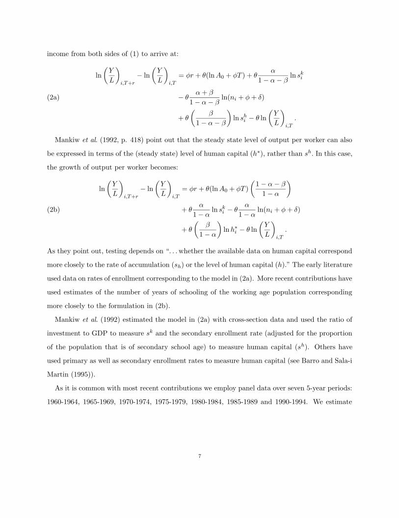
As they point out, testing depends on “. . . whether the available data on human capital correspond

more closely to the rate of accumulation (sh) or the level of human capital (h).” The early literature

used data on rates of enrollment corresponding to the model in (2a). More recent contributions have

used estimates of the number of years of schooling of the working age population corresponding

more closely to the formulation in (2b).

Mankiw et al. (1992) estimated the model in (2a) with cross-section data and used the ratio of

investment to GDP to measure sk and the secondary enrollment rate (adjusted for the proportion

of the population that is of secondary school age) to measure human capital (sh). Others have

used primary as well as secondary enrollment rates to measure human capital (see Barro and Sala-i

Martin (1995)).

As it is common with most recent contributions we employ panel data over seven 5-year periods:

1960-1964, 1965-1969, 1970-1974, 1975-1979, 1980-1984, 1985-1989 and 1990-1994. We estimate

7

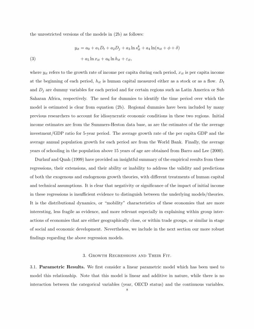
the unrestricted versions of the models in (2b) as follows:

yit = a0 + a1Dt + a2Dj + a3 ln skit + a4 ln(nit + φ + δ)

+ a5 ln xit + a6 ln hit + εit,(3)

where yit refers to the growth rate of income per capita during each period, xit is per capita income

at the beginning of each period, hit is human capital measured either as a stock or as a flow. Dt

and Dj are dummy variables for each period and for certain regions such as Latin America or Sub

Saharan Africa, respectively. The need for dummies to identify the time period over which the

model is estimated is clear from equation (2b). Regional dummies have been included by many

previous researchers to account for idiosyncratic economic conditions in these two regions. Initial

income estimates are from the Summers-Heston data base, as are the estimates of the the average

investment/GDP ratio for 5-year period. The average growth rate of the per capita GDP and the

average annual population growth for each period are from the World Bank. Finally, the average

years of schooling in the population above 15 years of age are obtained from Barro and Lee (2000).

Durlauf and Quah (1999) have provided an insightful summary of the empirical results from these

regressions, their extensions, and their ability or inability to address the validity and predictions

of both the exogenous and endogenous growth theories, with different treatments of human capital

and technical assumptions. It is clear that negativity or significance of the impact of initial income

in these regressions is insufficient evidence to distinguish between the underlying models/theories.

It is the distributional dynamics, or “mobility” characteristics of these economies that are more

interesting, less fragile as evidence, and more relevant especially in explaining within group inter-

actions of economies that are either geographically close, or within trade groups, or similar in stage

of social and economic development. Nevertheless, we include in the next section our more robust

findings regarding the above regression models.

3. Growth Regressions and Their Fit.

3.1. Parametric Results. We first consider a linear parametric model which has been used to

model this relationship. Note that this model is linear and additive in nature, while there is no

interaction between the categorical variables (year, OECD status) and the continuous variables.8

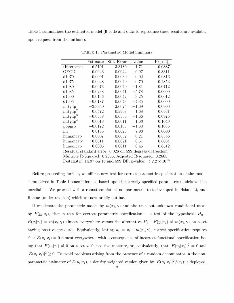
Table 1 summarizes the estimated model (R code and data to reproduce these results are available

upon request from the authors).

Table 1. Parametric Model Summary

Estimate Std. Error t value Pr(>|t|)(Intercept) 6.5101 3.8180 1.71 0.0887OECD −0.0043 0.0044 −0.97 0.3311d1970 0.0001 0.0039 0.02 0.9816d1975 0.0028 0.0040 0.70 0.4853d1980 −0.0073 0.0040 −1.81 0.0712d1985 −0.0238 0.0041 −5.78 0.0000d1990 −0.0136 0.0042 −3.25 0.0012d1995 −0.0187 0.0043 −4.35 0.0000initgdp −3.3940 2.0025 −1.69 0.0906initgdp2 0.6572 0.3908 1.68 0.0931initgdp3 −0.0558 0.0336 −1.66 0.0975initgdp4 0.0018 0.0011 1.63 0.1043popgro −0.0172 0.0105 −1.63 0.1035inv 0.0185 0.0023 7.93 0.0000humancap 0.0007 0.0032 0.21 0.8366humancap2 0.0011 0.0021 0.51 0.6084humancap3 0.0005 0.0011 0.45 0.6512Residual standard error: 0.026 on 599 degrees of freedomMultiple R-Squared: 0.2856, Adjusted R-squared: 0.2665F-statistic: 14.97 on 16 and 599 DF, p-value: < 2.2 × 1016

Before proceeding further, we offer a new test for correct parametric specification of the model

summarized in Table 1 since inference based upon incorrectly specified parametric models will be

unreliable. We proceed with a robust consistent nonparametric test developed in Hsiao, Li, and

Racine (under revision) which we now briefly outline.

If we denote the parametric model by m(xi, γ) and the true but unknown conditional mean

by E(yi|xi), then a test for correct parametric specification is a test of the hypothesis H0 :

E(yi|xi) = m(xi, γ) almost everywhere versus the alternative H1 : E(yi|xi) 6= m(xi, γ) on a set

having positive measure. Equivalently, letting ui = yi − m(xi, γ), correct specification requires

that E(ui|xi) = 0 almost everywhere, with a consequence of incorrect functional specification be-

ing that E(ui|xi) 6= 0 on a set with positive measure, or, equivalently, that [E(ui|xi)]2 = 0 and

[E(ui|xi)]2 ≥ 0. To avoid problems arising from the presence of a random denominator in the non-

parametric estimator of E(ui|xi), a density weighted version given by [E(ui|xi)]2f(xi) is deployed.

9

To test whether E(ui|xi) = 0 holds over the entire support of the regression function, the statistic

Idef= E{[E(ui|xi)]

2f(xi)} ≥ 0 is chosen. Note that I = 0 if and only if H0 is true, and I therefore

serves as a valid candidate for testing H0. The sample analogue of I is obtained by replacing ui

with the residuals obtained from the parametric null model, ui = yi − m(xi, γ), and by replacing

E(ui|xi) and f(xi) with their consistent kernel estimators, while the null distribution of the statistic

is obtained via resampling methods (‘wild-bootstrapping’). This test is directly applicable to the

problem at hand involving a mix of discrete and continuous data. The test has been shown to

have correct size and, being consistent, to possess good power properties against a wide class of

alternative models (see Hsiao, Li, Racine (under revision) for further details).

Applying this test to the parametric model summarized in Table 1 yields a p-value of 4.07087×

10−06. Unsurprisingly, this is extremely strong evidence against the null and indicates parametric

misspecification; See Durlauf and Johnson (1995) for similar findings based on other methods.

Given that we reject the null of (this) parametric specification, and given the presence of both

discrete and continuous data, we choose to proceed with a rather new nonparametric approach.

3.2. Nonparametric Results. For what follows, we consider a fully nonparametric local linear

specification using the estimator of Li and Racine (2004) that permits us to model the mix of discrete

and continuous data types found in the present context. We summarize the nonparametric results

using partial regression plots. These plots simply present the estimated multivariate regression

function via a series of bivariate plots in which the regressors not appearing on the horizontal

axis of a given plot have been held constant at their respective medians. That is, if we wish to

present the nonparametric regression of y on x1, x2, and x3, we plot y versus E(x1, x2, x3), y

versus E(x1, x2, x3), and y versus E(x1, x2, x3) where the bar denotes a median which allows one

to visualize the multivariate regression surface via a series of two-dimensional plots. One of the

appealing features of this approach is that it permits direct comparison of the parametric and

nonparametric results.

The profiles presented in figures 1 and 2 are constructed using our panel of 616 observations in

the following manner. First, least-squares cross-validation is used to obtain the appropriate band-

widths for the discrete and continuous regressors (see Li and Racine (2004) for details). Next we10

generate and plot the partial regression relationships between GDP Growth (Y ) and each contin-

uous explanatory variable holding the remaining continuous variables constant at their respective

medians (year = 1980, initial GDP = 7.8, population growth = -2.6, investment = -1.8, human

capital = 1.4 respectively). We also plot the partial parametric regression surfaces, and we consider

separate plots for OECD versus Non-OECD members.

Our nonparametric approach allows for interactions among all variables and also allows for

nonlinearities in and among all variables. Furthermore, the method has two defining features; i) if

the underlying relationship is linear in a variable(s) then the cross-validated smoothing parameter

is capable of automatically detecting this; ii) the method has better finite-sample properties than

the popular local constant kernel estimator, in particular, it is minimax efficient and is known to

possess one of the best boundary correction methods available. A summary of the particulars of

the nonparametric method for this panel (bandwidths and so forth) are available upon request from

the authors.

In the literature on growth convergence a great deal of attention has been paid to the relationship

between GDP Growth and Initial GDP. This relationship is given in the first plot in Figure 1. It

is clear that as Initial GDP rises, ceteris paribus, GDP growth falls. This would seem to offer

evidence in favor of “β-convergence” As Durlauf and Quah (1999), point out, however, this is not

evidence necessarily in favor of the traditional exogenous technical change, Solow-Swan model and

its extended forms. A negative “coefficient” of initial GDP is not empirically incompatible with

sometimes radically different theories.

An interesting feature arises when considering the conditional relationship between GDP growth

and population growth for OECD versus Non-OECD countries. Note that for OECD countries,

population growth “hurts” GDP growth. However, for Non-OECD countries, low levels of popu-

lation growth are beneficial while only high levels hurt growth. This is a reflection of an apparent

threshold level for population size which may support economic advancement. Many smaller and

economically less developed countries consider their population size to be a handicap in supporting

major industrial developments and investment.

These graphs make clear the importance of decomposition by country groups. Aggregating

these countries hides the very different impact that each group has experienced from investment,

11

-0.08

-0.06

-0.04

-0.02

0

0.02

0.04

0.06

0.08

0.1

6 6.5 7 7.5 8 8.5 9 9.5

GD

P G

row

th R

ate

Initial GDP

GDP Growth Versus Initial GDP

KernelLinear

-0.08

-0.06

-0.04

-0.02

0

0.02

0.04

0.06

0.08

0.1

-3 -2.9 -2.8 -2.7 -2.6 -2.5 -2.4

GD

P G

row

th R

ate

Population Growth

GDP Growth Versus Population Growth

KernelLinear

-0.08

-0.06

-0.04

-0.02

0

0.02

0.04

0.06

0.08

0.1

-3.5 -3 -2.5 -2 -1.5 -1

GD

P G

row

th R

ate

Investment

GDP Growth Versus Investment

KernelLinear

-0.08

-0.06

-0.04

-0.02

0

0.02

0.04

0.06

0.08

0.1

-1 -0.5 0 0.5 1 1.5 2

GD

P G

row

th R

ate

Human Capital

GDP Growth Versus Human Capital

KernelLinear

Figure 1. Nonparametric Partial Regression Plots for Non-OECD Countries.

population growth, and especially “human capital” upon its growth rates. While human capital

has an increasing and positive relation with growth for OECDs, it has a tenuous impact for Non-

OECDs. But a general association of low human capital and low growth rates is common to both

groups.

Given these observations, it is rather interesting that, for the parametric regression on all of

the countries, the OECD status (dummy) variable is insignificant. This underscores the dangers

inherent to the unquestioning use of linear models!

4. Evolution of Cross-Section Distributions

In view of the evident limitations of conditional means (or even variances) as vehicles for analysing

diversity (convergence!) within distributions, certainly of incomes, we now turn to the central

analysis of this paper based on the whole distribution of growth rates. The stylized facts concerning

the cross-section distributions of growth rates and their evolution are well laid out in Durlauf and

Quah (1999). The most important of these are a “polarization” effect being largely an evolution12

-0.08

-0.06

-0.04

-0.02

0

0.02

0.04

0.06

0.08

0.1

6 6.5 7 7.5 8 8.5 9 9.5

GD

P G

row

th R

ate

Initial GDP

GDP Growth Versus Initial GDP

KernelLinear

-0.08

-0.06

-0.04

-0.02

0

0.02

0.04

0.06

0.08

0.1

-3 -2.9 -2.8 -2.7 -2.6 -2.5 -2.4

GD

P G

row

th R

ate

Population Growth

GDP Growth Versus Population Growth

KernelLinear

-0.08

-0.06

-0.04

-0.02

0

0.02

0.04

0.06

0.08

0.1

-3.5 -3 -2.5 -2 -1.5 -1

GD

P G

row

th R

ate

Investment

GDP Growth Versus Investment

KernelLinear

-0.08

-0.06

-0.04

-0.02

0

0.02

0.04

0.06

0.08

0.1

-1 -0.5 0 0.5 1 1.5 2

GD

P G

row

th R

ate

Human Capital

GDP Growth Versus Human Capital

KernelLinear

Figure 2. Nonparametric Partial Regression Plots for OECD Countries.

into a “bipolar” world, and “churning” or what we prefer to call “within group mobility” which,

when examined in greater detail, points to possible “multimodality” and “clubs.”3

As noted earlier, several authors, including Binachi (1997), Jones (1997), and Quah (1993, 1997),

have examined the more interesting aspects of the dynamics in the distribution of growth rates in

light of the predictions of various growth models. This section’s analysis, and our main interest, is

in the same spirit. In particular, Binachi too obtains (different) nonparametric density estimates

for growth rate distributions at each point in time, whereas Quah (1997) examined the (relative)

per capita income distributions and their “transition” laws by analyzing transition probabilities

and their continuous counterpart, stochastic kernels. Examination of mobility (in any attribute)

has traditionally been conducted in two ways. Transition matrices (kernels) and indices defined

3Classification of countries by proximity or trade are given in Quah (1997) and others. We believe this questiondeserves greater attention and is perhaps best left to studies that consider multidimensional clustering which com-bine two different techniques. The multidimensionality aspects may be addressed in the manner of Maasoumi andJ. H. Jeong (1985) who considered composite measures of well being for the world, including per capita incomes.The clustering techniques of Hirschberg, Maasoumi and Slottje (2001) may then be applied to these multidimensionalindices.

13

over them, or inequality reducing measures based on “distances” between distributions and how

they evolve toward the “equal” distribution over time. Ideal indices of mobility based on the latter

approach are connected to those in the former, but a full understanding of the relations is not yet at

hand. See Maasoumi (1998) for an extended discussion. In addition, per capita income and growth

rates of incomes are at least statistically distinct (but surely related) variables. In comparing our

results with the complementary findings of Quah (1997), these distinctions must be born in mind.

Our findings reinforce the notion of divergence and polarization in both incomes and their growth

rates. We also find that some groupings of countries identify somewhat more uniform sets, but

neither identifies the causes of divergence in incomes or growth rates. Perhaps there is substance

in the view that “conditional convergence” is a rather vacuous concept. Of course there are causes

for the observed divergence.

4.1. Distribution Dynamics: Actual Growth Rates. For what follows, we focus attention

on the probability density function (PDF) and cumulative distribution function (CDF) of growth

rates, focusing on how the distribution of growth rates evolves over time and behaves with respect to

OECD status. Rather than presume that growth rates are generated from a known parametric fam-

ily of distributions, we use robust nonparametric methods capable of providing consistent estimates

of the unknown PDF and CDF. We elect to use kernel methods, and we estimate Rosenblatt-Parzen

type density estimates. Data-driven methods of bandwidth selection are employed, and bandwidths

are selected via likelihood cross-validation, which results in estimates that are close to the true

density in terms of the Kullback-Leibler information distance∫

f(y|x) log{f(y|x)/f(y|x)} dy where

f(y|x) represents the conditional density function (see Silverman (1986, page 53) and Hall (1987)).

We begin by modeling the PDF and CDF of the actual growth rates conditional on OECD

status (0/1) and year (1965, 1970, . . . ). Note that, by modeling the joint distribution of growth

rates, year, and OECD status and then conditioning on OECD status and year, we obtain a kernel

density estimate having improved finite-sample properties relative to the traditional univariate

kernel density estimate for growth rates for a particular year and OECD status (the latter using

only a subset of the data used to construct the former). The conditional density estimator found

in Hall et al. (forthcoming) is used due to the mix of continuous and discrete data present.14

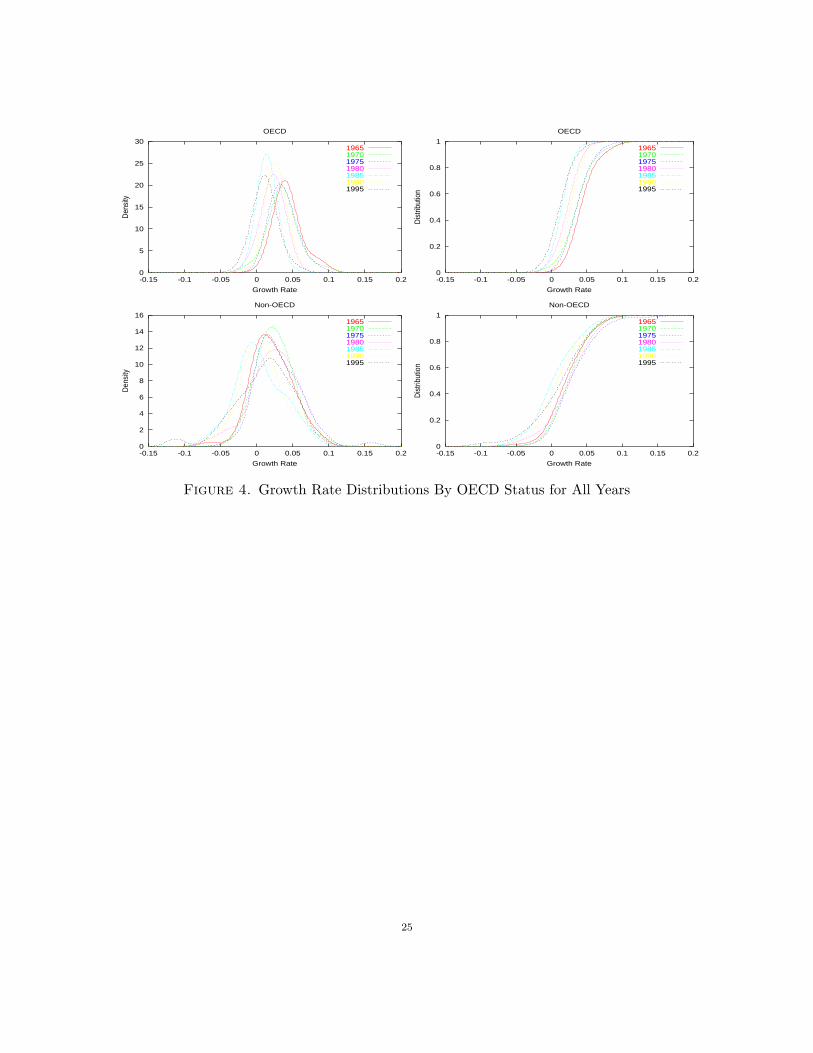
Figure 3 presents plots of the conditional PDF and CDF for all combinations of OECD status

and year, while Figure 4 presents a plot of all OECD distributions for all years and all Non-OECD

ones again for all years.

Several important features of these results may be noted:

(1) The growth distributions for the OECD and Non-OECD countries are very different, and

have remained very different from 1965 to 1995.

(2) The distribution for OECDs is less dispersed and is symmetrical, becoming more so over

time.

(3) The distribution for Non-OECDs is less symmetrical, and not converging to any particular

form, and becoming less concentrated. It appears to be forming a bimodality of its own

suggesting multimodality that, while not incompatible with parametric/traditional regres-

sion models, may be difficult for “regression techniques” to identify and examine. Within

group mobility in the Non-OECDs is made evident by these graphs. It is possible to derive

“mobility profiles” in the manner of Maasoumi and Zandvakili (1990), but we leave this to

future work.

(4) When combined, the previous two observations agree and further explain the often observed

and expanding multimodality in the world distribution of growth rates; For example see

Durlauf and Johnson (1995) who arrive at compatible inferences based on multiple regres-

sions and regression trees.

(5) Linton, Maasoumi and Whang (2002) consider welfare-theoretic bases for assessing the

relations between distributions. They propose subsampling based tests of First, Second

(and higher) Order Stochastic Dominance, FSD and SSD, respectively. Although one of us

has applied these tests to some of the cases in this paper, we partially agree with Quah

(1997) who suggests one has a census of all countries in the population here, not a sample.

Given this point of view, the following observations may be viewed as free from sampling

variation:

(a) In 1965-1970 OECD First Order Stochastically Dominates (FSD) the non-OECDs since

its CDF lies everywhere to the right of the latter. From 1975 there is no FSD ranking15

between these two groups, but there is Second Order SD (SSD) of OECDs over non-

OECDs through 1990 (with the possible exception of 1980). The order rankings are

inconclusive and almost identical for the 1980 and 1995 pair! It should be noted

that FSD is a very strong rank order and implies SSD. SSD obtains on the basis of

welfare functions that are increasing and concave (equality preferring). Thus, one

might conclude that the evolution of the non-OECD distribution has been positive,

and it is a higher degree of “convergence” of growth rates amongst the OECDs that

contributes to its SSD over the non-OECDs in later years. Some of these observations

are explained by the movement of China from a large population, low growth economy,

to a large population, high growth economy status. There is much “churning,” or

“exchange mobility,” and no “convergence” within the non-OECDs, and a tangible

convergence and “growth mobility” within the OECDs. There are clearly a minimum

of “two clubs” on the basis of growth rates alone. Similarly, Quah (1997) finds credible

evidence of relative per capita income “clubs” on the basis of geographical proximity,

as well as trading practices.

(b) Regarding the evolution of each group over time, again we find “a tale of two cities.”

OECDs have clearly “deteriorated” over time since the 1965, whereas the situation

for non-OECDs is far less clearcut. The OECD growth distribution in 1965 First

order dominates all other years. There is a clear break in the 1980s, resulting in a

gradual strengthening of this rank order as they evolve toward 1995. Note that this

period contained two recessions in the 1980s and early 90s. It would be interesting to

re-examine this hierarchy when more recent data become available. It is interesting

to note that, since FSD implies SSD, whatever small convergence in growth rates of

OECD, if any, it is not enough to topple the SSD ranking (greater “equality”) of earlier

years over the latter years.

(c) Regarding the non-OECDs, the only clearcut ranking is that 1985 is First order domi-

nated by every other year except 1995. Clearly this was not a “good” year for growth

globally. But, the differential development within this group is well reflected by a lack

16

of FSD amongst other years. It is possible that 1965 weakly Second order dominates

1995, yet another reflection of a lack of “convergence” in these distributions.

We are in fact able to quantify the magnitudes of these movements between entire dis-

tributions! Thus we will report entropy distances and related tests in a subsequent section

which shed light on the “magnitude” of these distances and focus on convergence.

4.2. Distribution Dynamics: Nonparametric Fitted Growth Rates. Our nonparametric

regressions have produced what might be considered robust fitted values of the growth rates in the

plane of the most popular conditioning variables.

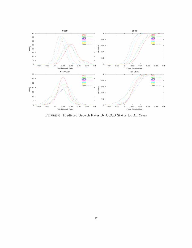
We present the PDF and CDF of these “fitted” or estimated growth rates. Plots of these

conditional PDFs and CDFs for all combinations of OECD status and year are followed, finally,

by plots of all OECD distributions for all years as well as all Non-OECD countries for all years.

The FSD and SSD rankings are similar to the “raw” growth distributions. The evolution of growth

rates, as predicted by popular explanatory variables and free of “residual sources,” tends to conform

to the “unconditional” evolution analysis provided in the previous section. Several caveats are in

order, however:

(1) The FSD rankings between the OECD and others is even stronger than for raw growth

rates, becoming less strong toward 1980, whereby it is only a SSD ranking with decreasing

strength toward 1995 where there may be at most a Third Order SD ranking between them.

“Bipolarity” is surely not questioned.

(2) All of our previous statements regarding the “time path” of these distributions for each

group are intact, but somewhat stronger rankings are possible for the non-OECD distri-

butions over time (compare this with generally consistent results of Quah (1997) for per

capita incomes, and Durlauf and Quah (1999)).

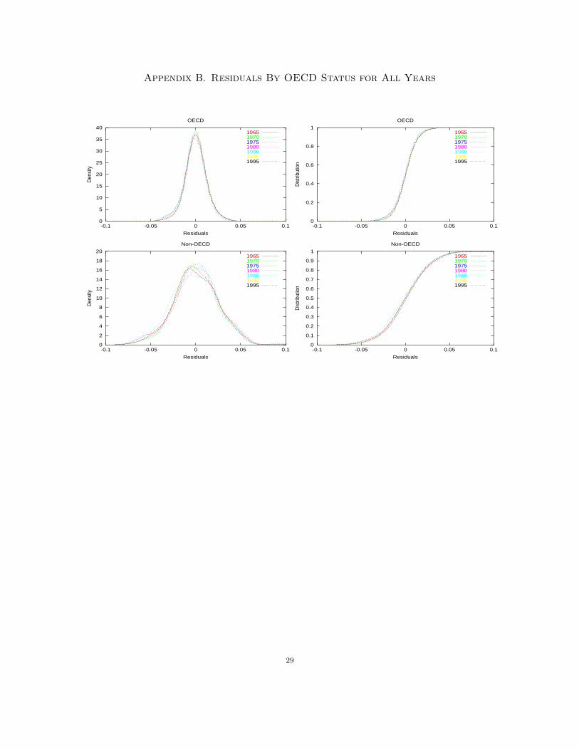
4.3. Residual Growth Rates by OECD Status for all Years. Appendix A presents results

based on the distribution of our nonparametric regression “residuals,” organized in the same manner

as the last two sections. These residuals may be regarded as “conditional” growth rates in the usual

meaning of conditioning in econometrics. The residuals are growth rates after controlling for the

influence of conditioning variables. Of course this control is only achieved on the mean of the17

growth rates, and the variables may continue to impact other distributional characteristics. This

residual analysis is valuable since our residuals are robust to functional forms and any evidence of

“convergence” of their distributions may be interpreted as evidence of “conditional convergence.”4

We summarize as follows:

(1) There is no FSD between the OECD and non-OECD groups. There is generally no SSD

either, with the possibility of week SSD or higher orders for some later years. Once the

mean differences due to conditional variables are removed, uniform ranking of these groups

by dominance criteria vanishes. Interestingly, even the dispersion aspects of these two

distributions are generally not sufficiently different to produce higher order (SSD) rankings.

This is evidence in favor of “conditional convergence” in the sense developed in this paper.5

(2) The “fit” is generally good for the regressions, but less good for non-OECD data because

of their heterogeneity.

(3) There is not much to separate these distributions over the successive five year intervals.

The fit is equally good (bad) for each cross-section.

Also, note that the residuals are effectively ‘smoothed’ over time so that differences in the residual

series are negligible for different time periods.

5. Entropy Measures of Distributional Distance

In this section we provide a formal quantification of the distributional distances and evolu-

tions observed in the last section. This is done by using a metric entropy measure suggested in

Granger et al. (forthcoming).6 Any entropy measure is useful as an indicator of divergence from

the uniform distribution, and is thus a measure of “equality,” or concentration in the corresponding

distribution. The characterization of a density afforded by entropies is only a little short of that

provided by characteristic functions. Thus entropies are generally superior to other moment-based

4We are sympathetic, however, to the view that considers “conditional convergence” as rather lacking in meaning orconsequence, especially relative to substantive theories and hypotheses which initially motivated this area of research.5It is worth noting that “strong” non-uniform rankings are not ruled out. There do exist cardinal (welfare) criteriaaccording to which these distributions may be ranked. Variance is one such criterion, however unlikely in thissituation.6For comparison purposes, we also computed the Kullback-Leibler divergence measure. These were removed to savespace but give consistent results. The KL measure is the most popular index of divergence between distributions,but it is not a metric and unsuited for precisely the type of comparisons of “distances” we need to make in thisapplication.

18

criteria. Unfortunately, Shannon’s popular entropy is not a metric and thus fails to be useful for

multiple comparisons, exemplified by our application here where several years and/or groups of

distributions are being compared. Granger et al. (forthcoming) developed a normalized entropy

measure of “dependence” that has several desirable properties as well as being a proper distance

metric. Some of these properties are briefly enumerated here for convenience. A measure of simi-

larity/distance/dependence for a pair of random variables X and Y may be required to satisfy the

following six “ideal” properties:

(i) It is well defined for both continuous and discrete variables. (ii) It is normalized to zero if

X and Y are identical, and is conveniently normalized to lie between 0 and +1. (iii) The modulus

of the measure is equal to unity if there is a measurable exact (nonlinear) relationship, Y = g(X)

say, between the random variables. This is useful in our use of this measure for assessing the fit of

regressions. (iv) It is equal to or has a simple relationship with the (linear) correlation coefficient

in the case of a bivariate normal distribution. Again, this is useful in our use of this measure

for assessing the fit of regressions. (v) It is metric, that is, it is a true measure of “distance”

and not just of divergence. (vi) The measure is invariant under continuous and strictly increasing

transformations h(·). This is useful since X and Y are independent if and only if h(X) and h(Y )

are independent. Invariance is important since otherwise clever or inadvertent transformations

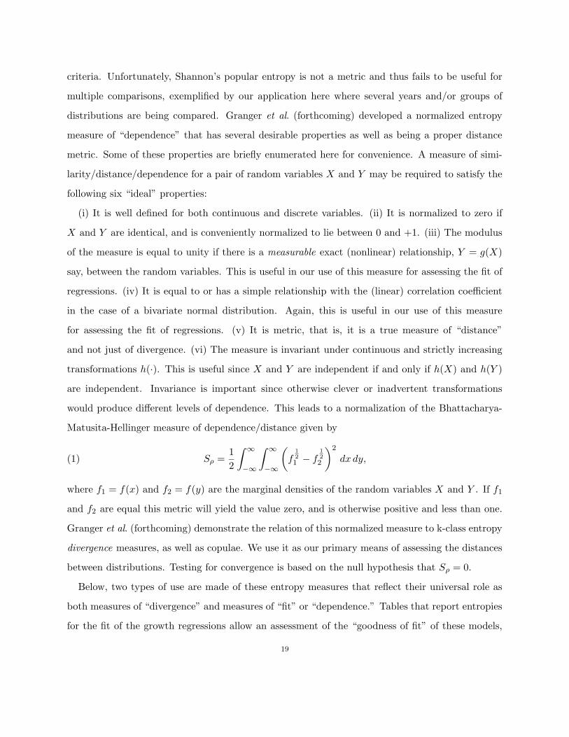
would produce different levels of dependence. This leads to a normalization of the Bhattacharya-

Matusita-Hellinger measure of dependence/distance given by

(1) Sρ =1

2

∫∞

−∞

∫∞

−∞

(f

1

2

1− f

1

2

2

)2

dx dy,

where f1 = f(x) and f2 = f(y) are the marginal densities of the random variables X and Y . If f1

and f2 are equal this metric will yield the value zero, and is otherwise positive and less than one.

Granger et al. (forthcoming) demonstrate the relation of this normalized measure to k-class entropy

divergence measures, as well as copulae. We use it as our primary means of assessing the distances

between distributions. Testing for convergence is based on the null hypothesis that Sρ = 0.

Below, two types of use are made of these entropy measures that reflect their universal role as

both measures of “divergence” and measures of “fit” or “dependence.” Tables that report entropies

for the fit of the growth regressions allow an assessment of the “goodness of fit” of these models,

19

and represent new results in their own right. Since our regressions are not linear, the traditional

measures of correlation and linear dependence, such as R2, are clearly inadequate. Thus in these

tables we offer the first robust dependence results for the fit of the traditional growth regression

variables.7

Table 2. Shannon’s Entropy (-∫∞

−∞f(x) ln(f(x)) dx).

OECD 1965 1970 1975 1980 1985 1990 1995Actual Growth Rate -2.432 -2.324 -2.479 -2.584 -2.774 -2.686 -2.532Parametric Fit -3.533 -3.561 -3.582 -3.766 -3.733 -3.784 -3.768Nonparametric Fit -2.692 -2.689 -2.745 -3.027 -3.113 -3.092 -3.091Parametric Residual -2.668 -2.607 -2.683 -2.706 -2.806 -2.725 -2.669Nonparametric Residual -3.012 -2.956 -3.031 -3.012 -3.039 -3.054 -2.948Non-OECD 1965 1970 1975 1980 1985 1990 1995Actual Growth Rate -2.077 -2.158 -2.029 -1.966 -1.942 -1.970 -1.800Parametric Fit -2.839 -2.855 -2.804 -2.881 -2.867 -2.868 -2.814Nonparametric Fit -2.871 -2.738 -2.525 -2.812 -2.729 -2.641 -2.226Parametric Residual -2.104 -2.195 -2.147 -2.054 -2.055 -2.087 -2.048Nonparametric Residual -2.262 -2.314 -2.281 -2.213 -2.229 -2.262 -2.267

In terms of Shannon’s entropy (reported in Table 2), the actual growth rate distributions for

OECD were becoming somewhat more concentrated until 1985, whereafter increasing in dispersion

levels of 1965. For non-OECDs the increase in dispersion/inequality of growth rates is a steady

pattern. Neither of these changes are “large” in absolute value (but see below for statistical evalu-

ation).

Table 3. KL Entropy (∫∞

−∞f(x) ln(f(x)/g(x)) dx) (f(x)=Non-OECD,

g(x)=OECD). The values in brackets are the 90th and 95th percentiles ob-tained under the null of no difference between OECD and Non-OECD countries.Kernel Evaluation of KL Entropy: OECD versus Non-OECD

1965 1970 1975 1980 1985 1990 1995Actual Growth Rate 0.803 0.160 0.383 0.630 1.378 1.237 0.580

[0.182, 0.212] [0.157, 0.187] [0.184, 0.211] [0.190, 0.228] [0.194, 0.235] [0.174, 0.216] [0.323, 0.352]Parametric Fit 1.623 1.628 1.064 1.098 1.270 1.669 1.572

[0.294, 0.340] [0.255, 0.304] [0.261, 0.304] [0.270, 0.339] [0.284, 0.360] [0.290, 0.346] [0.301, 0.349]Nonparametric Fit 1.154 0.504 0.476 0.085 0.512 0.950 1.047

[0.240, 0.291] [0.147, 0.182] [0.226, 0.284] [0.100, 0.128] [0.128, 0.154] [0.224, 0.272] [0.349, 0.424]

7We compute all entropy measures in the following manner: (i) Compute the conditional Rosenblatt-Parzen densityestimates with covariates OECD status and Year via cross-validation. (ii) Generate a grid in [−0.25, 0.25] havinggrain 0.001 (there are 501 points on this grid). (iii) Evaluate the Rosenblatt-Parzen kernel estimator on the grid of

501 points. Note that at the edges of the grid f(x|OECD, Year) = 0.0. (iv) Evaluate each respective entropy vianumerical quadrature.

20

Table 4. Sρ Entropy (1

2

∫∞

−∞[√

f(x) −√

g(x)]2 dx) (f(x)=Non-OECD,

g(x)=OECD). The values in brackets are the 90th and 95th percentiles ob-tained under the null of no difference between OECD and Non-OECD countries.

1965 1970 1975 1980 1985 1990 1995Actual Growth Rate 0.127 0.035 0.069 0.089 0.182 0.180 0.112

[0.040, 0.048] [0.032, 0.040] [0.043, 0.049] [0.039, 0.044] [0.040, 0.047] [0.038, 0.045] [0.054, 0.065]Parametric Fit 0.259 0.232 0.156 0.147 0.174 0.175 0.198

[0.061, 0.070] [0.053, 0.063] [0.056, 0.068] [0.059, 0.069] [0.057, 0.067] [0.059, 0.069] [0.060, 0.069]Nonparametric Fit 0.252 0.111 0.067 0.015 0.077 0.141 0.143

[0.043, 0.051] [0.031, 0.038] [0.042, 0.051] [0.022, 0.029] [0.027, 0.032] [0.038, 0.044] [0.069, 0.077]

In table 2 we note that the distances Sρ (also KL divergences not reported here) between OECD

and others is significant at the 95% level for every date except 1970. Over time, we see that these

distances declined in the 1960s, thereafter growing steadily until 1990, but seem to have declined

in 1990-1995.

Table 5. Sρ Entropy (1

2

∫∞

−∞[√

f(x) −√

g(x)]2 dx) (f(x)=Actual, g(x)=Predicted).

OECD 1965 1970 1975 1980 1985 1990 1995Parametric 0.196 0.232 0.228 0.240 0.173 0.215 0.243Nonparametric 0.020 0.041 0.019 0.047 0.037 0.038 0.069Non-OECD 1965 1970 1975 1980 1985 1990 1995Parametric 0.140 0.117 0.143 0.188 0.183 0.174 0.209Nonparametric 0.125 0.080 0.062 0.155 0.154 0.103 0.043

Table 3 reports the “goodness of fit” values for the parametric as well as our own nonparametric

models. For OECDs, the parametric fit is much better than the nonparametric one. This is

predictable from the relative homogeneity in this group. The nonparametric fit is much better for

the non-OECDs, but deteriorates in the later parts of the sample.

Table 6. Sρ Entropy (1

2

∫∞

−∞[√

f(x) −√

g(x)]2 dx) (f(x)=Yeart, g(x)=Yeart+5).The values in brackets are the 90th and 95th percentiles obtained under the null ofno difference over time.

1965-70 1970-75 1975-80 1980-85 1985-90 1990-95Pooled 0.003 0.006 0.014 0.032 0.008 0.008

[0.013, 0.016] [0.014, 0.017] [0.015, 0.017] [0.014, 0.017] [0.015, 0.017] [0.015, 0.016]OECD 0.017 0.009 0.071 0.037 0.074 0.093

[0.037, 0.045] [0.038, 0.045] [0.038, 0.048] [0.036, 0.044] [0.039, 0.045] [0.036, 0.045]Non-OECD 0.007 0.011 0.022 0.047 0.010 0.023

[0.026, 0.030] [0.025, 0.029] [0.027, 0.030] [0.026, 0.029] [0.026, 0.030] [0.026, 0.030]

21

Table 4 corresponds to our earlier graphical analysis of evolution through time. For the pooled

sample, only the distances between 1980-85 are significant at 95% level. These distances first

increase to 1985, but thereafter become small again. By these indices, one would infer “conver-

gence” except in 1980-85, demonstrating the difficulty of analyzing distributional dynamics by

strong/complete but non-uniform criteria. In the absence of uniform SD rankings, there will exist

some “criterion function” which may reverse the conclusion of “convergence,” by another criterion.

This may explain some of the quandary in the current literature with different conclusions being

reached by different authors on the question of convergence.

By either measure of divergence, the OECD countries moved forward by small amounts in the late

1960s and early 70s, but changing significantly in later periods (except for 1980-85). For the non-

OECD growth distributions, on the other hand, the two measures suggest that their distributions

have been changing slowly, indeed only significantly so in 1980-85.

The magnitude of changes over time are generally much larger for OECDs than others (‘the rich

get richer and the poor get poorer’). These observations add credence to those in Durlauf and

Quah (1999) and elsewhere, that the most interesting aspects of the growth phenomenon appear

to be in different distributional dynamics and mobility profiles of different country groups, rather

than in the growth regressions.

Appendix C reports similar analysis for “conditional growth rates,” i.e., the residuals of both

the parametric and nonparametric growth regressions. Our earlier observations are confirmed by

these entropy tests.

(1) The “fit” is generally good for the regressions, but less good for non-OECD data because

of their less homogeneous membership.

(2) There is not much to separate these distributions over the successive five year intervals. The

fit is equally good (bad) for each cross-section. Also, note that the residuals are effectively

‘smoothed’ over time so that differences in the residual series are negligible for different

time periods.

(3) There is no significant change in these residual growth distributions at the 95% level, and

almost always, even at the 90% level (the exception is, again, 1980-85 for OECDs which

are significant at the 90% level).22

(4) There is a further interpretation of these entropy measures of dynamic residual movements.

Following Granger et al. (forthcoming), the entropies in this context may be regarded as

robust measures of possibly nonlinear serial dependence. Accordingly, our results indicate

that there is no evidence of significant serial dependence of residuals between these five year

periods.

A summary of the conditional and unconditional (“actual”) growth rates and their distributional

characteristics is given in tables 11 and 12 of Appendix C.

6. Conclusions

Employing nonparametric kernel density and regression techniques, we have examined the oth-

erwise traditional growth relationship and given new entropy measures of fit, as well as residual

correlation for them. We have identified distinct effects of the major conditioning variables on the

growth rates of different groups of countries. This leaves very little doubt that separate models are

required to examine different groups of countries.

We have further examined the dynamics of cross-section distributions of actual growth rates,

as well as “conditional” and “fitted” growth rates. Our study of these dynamics was based on

Stochastic Dominance rankings, as well as tests based on entropy distances which shed further

light on the mobility between and within groups of countries. Our robust findings tend to confirm

the hypotheses of “convergence clubs” and polarization.

We agree with the conclusions of Durlauf and Quah (1999) that future work needs to address

more successfully the need for modeling of cross-country interactions and remain consistent with the

rich distributional dynamics observed here, and studied in the mobility literature as, for example,

in Maasoumi and Zandvakili (1990). There is also a need to extend the scope of this field by

considering other attributes of well-being than per capita incomes, and connecting to the literature

which deals with its related issues; see, for example, Hirschberg et al. (2001), and Maasoumi and

Jeong (1985).

23

0

5

10

15

20

25

-0.15 -0.1 -0.05 0 0.05 0.1 0.15 0.2

Densi

ty

Growth Rate

1965

OECDNon-OECD

0

0.2

0.4

0.6

0.8

1

-0.15 -0.1 -0.05 0 0.05 0.1 0.15 0.2

Distrib

ution

Growth Rate

1965

OECDNon-OECD

0

2

4

6

8

10

12

14

16

18

20

-0.15 -0.1 -0.05 0 0.05 0.1 0.15 0.2

Densi

ty

Growth Rate

1970

OECDNon-OECD

0

0.2

0.4

0.6

0.8

1

-0.15 -0.1 -0.05 0 0.05 0.1 0.15 0.2

Distrib

ution

Growth Rate

1970

OECDNon-OECD

0

5

10

15

20

25

-0.15 -0.1 -0.05 0 0.05 0.1 0.15 0.2

Densi

ty

Growth Rate

1975

OECDNon-OECD

0

0.2

0.4

0.6

0.8

1

-0.15 -0.1 -0.05 0 0.05 0.1 0.15 0.2

Distrib

ution

Growth Rate

1975

OECDNon-OECD

0

5

10

15

20

25

-0.15 -0.1 -0.05 0 0.05 0.1 0.15 0.2

Distrib

ution

Growth Rate

1980

OECDNon-OECD

0

0.2

0.4

0.6

0.8

1

-0.15 -0.1 -0.05 0 0.05 0.1 0.15 0.2

Distrib

ution

Growth Rate

1980

OECDNon-OECD

0

5

10

15

20

25

30

-0.15 -0.1 -0.05 0 0.05 0.1 0.15 0.2

Densi

ty

Growth Rate

1985

OECDNon-OECD

0

0.2

0.4

0.6

0.8

1

-0.15 -0.1 -0.05 0 0.05 0.1 0.15 0.2

Distrib

ution

Growth Rate

1985

OECDNon-OECD

0

5

10

15

20

25

30

-0.15 -0.1 -0.05 0 0.05 0.1 0.15 0.2

Densi

ty

Growth Rate

1990

OECDNon-OECD

0

0.2

0.4

0.6

0.8

1

-0.15 -0.1 -0.05 0 0.05 0.1 0.15 0.2

Distrib

ution

Growth Rate

1990

OECDNon-OECD

0

5

10

15

20

25

-0.15 -0.1 -0.05 0 0.05 0.1 0.15 0.2

Densi

ty

Growth Rate

1995

OECDNon-OECD

0

0.2

0.4

0.6

0.8

1

-0.15 -0.1 -0.05 0 0.05 0.1 0.15 0.2

Distrib

ution

Growth Rate

1995

OECDNon-OECD

Figure 3. Growth Rate Distributions by Year and OECD Status

24

0

5

10

15

20

25

30

-0.15 -0.1 -0.05 0 0.05 0.1 0.15 0.2

Den

sity

Growth Rate

OECD

1965197019751980198519901995

0

0.2

0.4

0.6

0.8

1

-0.15 -0.1 -0.05 0 0.05 0.1 0.15 0.2

Dis

tribu

tion

Growth Rate

OECD

1965197019751980198519901995

0

2

4

6

8

10

12

14

16

-0.15 -0.1 -0.05 0 0.05 0.1 0.15 0.2

Den

sity

Growth Rate

Non-OECD

1965197019751980198519901995

0

0.2

0.4

0.6

0.8

1

-0.15 -0.1 -0.05 0 0.05 0.1 0.15 0.2

Dis

tribu

tion

Growth Rate

Non-OECD

1965197019751980198519901995

Figure 4. Growth Rate Distributions By OECD Status for All Years

25

0

5

10

15

20

25

30

35

-0.04 -0.02 0 0.02 0.04 0.06 0.08 0.1

Densi

ty

Fitted Growth Rate

1965

OECDNon-OECD

0

0.2

0.4

0.6

0.8

1

-0.04 -0.02 0 0.02 0.04 0.06 0.08 0.1

Distrib

ution

Fitted Growth Rate

1965

OECDNon-OECD

0

5

10

15

20

25

-0.04 -0.02 0 0.02 0.04 0.06 0.08 0.1

Densi

ty

Fitted Growth Rate

1970

OECDNon-OECD

0

0.2

0.4

0.6

0.8

1

-0.04 -0.02 0 0.02 0.04 0.06 0.08 0.1

Distrib

ution

Fitted Growth Rate

1970

OECDNon-OECD

0

5

10

15

20

25

30

-0.04 -0.02 0 0.02 0.04 0.06 0.08 0.1

Densi

ty

Fitted Growth Rate

1975

OECDNon-OECD

0

0.1

0.2

0.3

0.4

0.5

0.6

0.7

0.8

0.9

1

-0.04 -0.02 0 0.02 0.04 0.06 0.08 0.1

Distrib

ution

Fitted Growth Rate

1975

OECDNon-OECD

0

5

10

15

20

25

30

35

-0.04 -0.02 0 0.02 0.04 0.06 0.08 0.1

Distrib

ution

Fitted Growth Rate

1980

OECDNon-OECD

0

0.2

0.4

0.6

0.8

1

-0.04 -0.02 0 0.02 0.04 0.06 0.08 0.1

Distrib

ution

Fitted Growth Rate

1980

OECDNon-OECD

0

5

10

15

20

25

30

35

40

-0.04 -0.02 0 0.02 0.04 0.06 0.08 0.1

Densi

ty

Fitted Growth Rate

1985

OECDNon-OECD

0

0.2

0.4

0.6

0.8

1

-0.04 -0.02 0 0.02 0.04 0.06 0.08 0.1

Distrib

ution

Fitted Growth Rate

1985

OECDNon-OECD

0

5

10

15

20

25

30

35

40

-0.04 -0.02 0 0.02 0.04 0.06 0.08 0.1

Densi

ty

Fitted Growth Rate

1990

OECDNon-OECD

0

0.2

0.4

0.6

0.8

1

-0.04 -0.02 0 0.02 0.04 0.06 0.08 0.1

Distrib

ution

Fitted Growth Rate

1990

OECDNon-OECD

0

5

10

15

20

25

30

35

40

-0.04 -0.02 0 0.02 0.04 0.06 0.08 0.1

Densi

ty

Fitted Growth Rate

1995

OECDNon-OECD

0

0.2

0.4

0.6

0.8

1

-0.04 -0.02 0 0.02 0.04 0.06 0.08 0.1

Distrib

ution

Fitted Growth Rate

1995

OECDNon-OECD

Figure 5. Nonparametric Fitted Growth Rates

26

0

5

10

15

20

25

30

35

40

-0.04 -0.02 0 0.02 0.04 0.06 0.08 0.1

Den

sity

Fitted Growth Rate

OECD

1965197019751980198519901995

0

0.2

0.4

0.6

0.8

1

-0.04 -0.02 0 0.02 0.04 0.06 0.08 0.1

Dis

tribu

tion

Fitted Growth Rate

OECD

1965197019751980198519901995

0

5

10

15

20

25

30

35

-0.04 -0.02 0 0.02 0.04 0.06 0.08 0.1

Den

sity

Fitted Growth Rate

Non-OECD

1965197019751980198519901995

0

0.2

0.4

0.6

0.8

1

-0.04 -0.02 0 0.02 0.04 0.06 0.08 0.1

Dis

tribu

tion

Fitted Growth Rate

Non-OECD

1965197019751980198519901995

Figure 6. Predicted Growth Rates By OECD Status for All Years

27

Appendix A. Residuals By Year and OECD Status

0

5

10

15

20

25

30

35

40

-0.1 -0.05 0 0.05 0.1

Densi

ty

Residuals

1965

OECDNon-OECD

0

0.2

0.4

0.6

0.8

1

-0.1 -0.05 0 0.05 0.1

Distrib

ution

Residuals

1965

OECDNon-OECD

0

5

10

15

20

25

30

35

40

-0.1 -0.05 0 0.05 0.1

Densi

ty

Residuals

1970

OECDNon-OECD

0

0.2

0.4

0.6

0.8

1

-0.1 -0.05 0 0.05 0.1

Distrib

ution

Residuals

1970

OECDNon-OECD

0

5

10

15

20

25

30

35

40

-0.1 -0.05 0 0.05 0.1

Densi

ty

Residuals

1975

OECDNon-OECD

0

0.2

0.4

0.6

0.8

1

-0.1 -0.05 0 0.05 0.1

Distrib

ution

Residuals

1975

OECDNon-OECD

0

5

10

15

20

25

30

35

40

-0.1 -0.05 0 0.05 0.1

Distrib

ution

Residuals

1980

OECDNon-OECD

0

0.2

0.4

0.6

0.8

1

-0.1 -0.05 0 0.05 0.1

Distrib

ution

Residuals

1980

OECDNon-OECD

0

5

10

15

20

25

30

35

40

-0.1 -0.05 0 0.05 0.1

Densi

ty

Residuals

1985

OECDNon-OECD

0

0.2

0.4

0.6

0.8

1

-0.1 -0.05 0 0.05 0.1

Distrib

ution

Residuals

1985

OECDNon-OECD

0

5

10

15

20

25

30

35

40

-0.1 -0.05 0 0.05 0.1

Densi

ty

Residuals

1990

OECDNon-OECD

0

0.2

0.4

0.6

0.8

1

-0.1 -0.05 0 0.05 0.1

Distrib

ution

Residuals

1990

OECDNon-OECD

0

5

10

15

20

25

30

35

40

-0.1 -0.05 0 0.05 0.1

Densi

ty

Residuals

1995

OECDNon-OECD

0

0.2

0.4

0.6

0.8

1

-0.1 -0.05 0 0.05 0.1

Distrib

ution

Residuals

1995

OECDNon-OECD

28

Appendix B. Residuals By OECD Status for All Years

0

5

10

15

20

25

30

35

40

-0.1 -0.05 0 0.05 0.1

Den

sity

Residuals

OECD

1965197019751980198519901995

0

0.2

0.4

0.6

0.8

1

-0.1 -0.05 0 0.05 0.1

Dis

tribu

tion

Residuals

OECD

1965197019751980198519901995

0

2

4

6

8

10

12

14

16

18

20

-0.1 -0.05 0 0.05 0.1

Den

sity

Residuals

Non-OECD

1965197019751980198519901995

0

0.1

0.2

0.3

0.4

0.5

0.6

0.7

0.8

0.9

1

-0.1 -0.05 0 0.05 0.1

Dis

tribu

tion

Residuals

Non-OECD

1965197019751980198519901995

29

Appendix C. Growth Rate Dynamics

Table 7. KL Entropy for Parametric Residuals (∫∞

−∞f(x) ln(f(x)/g(x)) dx)

(f(x)=Yeart, g(x)=Yeart+5). The values in brackets are the 90th and 95th per-centiles obtained under the null of no difference over time.

1965-70 1970-75 1975-80 1980-85 1985-90 1990-95OECD 0.020 0.019 0.012 0.053 0.010 0.037

[0.032, 0.039] [0.032, 0.040] [0.033, 0.039] [0.032, 0.038] [0.032, 0.039] [0.033, 0.040]Non-OECD 0.014 0.006 0.030 0.012 0.005 0.015

[0.025, 0.030] [0.025, 0.029] [0.025, 0.029] [0.026, 0.030] [0.026, 0.030] [0.026, 0.030]

Table 8. Sρ Entropy Dynamic for Parametric Residuals ( 1

2

∫∞

−∞[√

f(x) −√g(x)]2 dx ) (f(x)=Yeart, g(x)=Yeart+5). The values in brackets are the 90th

and 95th percentiles obtained under the null of no difference over time.

1965-70 1970-75 1975-80 1980-85 1985-90 1990-95OECD 0.006 0.004 0.003 0.013 0.003 0.009

[0.008, 0.009] [0.008, 0.010] [0.008, 0.010] [0.008, 0.009] [0.008, 0.010] [0.008, 0.010]Non-OECD 0.003 0.002 0.007 0.003 0.001 0.004

[0.006, 0.007] [0.006, 0.007] [0.006, 0.007] [0.006, 0.007] [0.006, 0.007] [0.006, 0.007]

Table 9. KL Entropy for Kernel Residuals (∫∞

−∞f(x) ln(f(x)/g(x)) dx)

(f(x)=Yeart, g(x)=Yeart+5). The values in brackets are the 90th and 95thpercentiles obtained under the null of no difference over time.

1965-70 1970-75 1975-80 1980-85 1985-90 1990-95OECD 0.008 0.009 0.004 0.005 0.014 0.013

[0.013, 0.016] [0.014, 0.017] [0.013, 0.017] [0.013, 0.016] [0.013, 0.016] [0.014, 0.016]Non-OECD 0.005 0.004 0.013 0.012 0.010 0.004

[0.012, 0.013] [0.011, 0.013] [0.011, 0.012] [0.011, 0.013] [0.012, 0.013] [0.011, 0.013]

30

Table 10. Sρ Entropy for Kernel Residuals ( 1

2

∫∞

−∞[√

f(x) −√

g(x)]2 dx)

(f(x)=Yeart, g(x)=Yeart+5). The values in brackets are the 90th and 95th per-centiles obtained under the null of no difference over time.

1965-70 1970-75 1975-80 1980-85 1985-90 1990-95OECD 0.002 0.002 0.001 0.001 0.003 0.003

[0.003, 0.004] [0.003, 0.004] [0.003, 0.004] [0.003, 0.004] [0.003, 0.004] [0.003, 0.004]Non-OECD 0.001 0.001 0.003 0.003 0.003 0.001

[0.003, 0.003] [0.003, 0.003] [0.003, 0.003] [0.003, 0.003] [0.003, 0.003] [0.003, 0.003]

Table 11. Actual Growth Rates Summary

Mean Median σ IQRYear OECD Non-OECD OECD Non-OECD OECD Non-OECD OECD Non-OECD

1965 0.044 0.022 0.039 0.020 0.018 0.028 0.015 0.0371970 0.037 0.025 0.035 0.025 0.021 0.025 0.017 0.0331975 0.037 0.031 0.033 0.025 0.016 0.031 0.022 0.0421980 0.022 0.023 0.022 0.027 0.013 0.032 0.012 0.0421985 0.014 0.003 0.014 -0.002 0.007 0.033 0.008 0.0411990 0.027 0.011 0.025 0.009 0.010 0.032 0.012 0.0341995 0.011 0.010 0.011 0.014 0.014 0.041 0.012 0.052

Table 12. Kernel Predicted Growth Rates Summary

Mean Median σ IQRYear OECD Non-OECD OECD Non-OECD OECD Non-OECD OECD Non-OECD

1965 0.042 0.020 0.041 0.020 0.015 0.011 0.017 0.0131970 0.037 0.022 0.038 0.021 0.015 0.013 0.018 0.0221975 0.035 0.026 0.032 0.028 0.014 0.018 0.018 0.0221980 0.023 0.022 0.022 0.023 0.008 0.012 0.011 0.0131985 0.018 0.010 0.018 0.012 0.007 0.013 0.008 0.0161990 0.025 0.014 0.021 0.014 0.007 0.016 0.009 0.0171995 0.013 0.012 0.011 0.015 0.007 0.028 0.009 0.031

31

References

[1] Azariadis, C. and A. Drazen (1990), “Threshold Externalities in Economic Development,” Quarterly Journal of

Economics, 501-526.

[2] Bianchi, M. (1997), “Testing for Convergence: Evidence from Nonparametric Multimodality Tests,” Journal of

Applied Econometrics, 12(4), 393-409.

[3] Barro, R. (1991), “Economic Growth in Cross Section of Countries” Quarterly Journal of Economics, CVI,

407-444.

[4] Barro, R. and Lee J-W (2000), “International Data on Educational Attainment: Updates and Implications”

Working paper No. 42, Center for International Development, Harvard University.

[5] Barro, R. and Sala-i-Martin, X (1995), Economic Growth, McGraw-Hill.

[6] Durlauf, S. N. and P. A. Johnson (1995), “Multiple Regimes and Cross-Country Growth Behavior,” Journal of

Applied Econometrics, 10, 365-384.

[7] Durlauf, S. N. and D. T. Quah (1999), “The New Empirics of Economic Growth,” Chapter 4, of J.B. Taylor and

M. Woodford (eds.), Handbook of Macroeconomics I, Elsevier sciences, 235-308.

[8] Fiaschi, D. and A. Lavezzi (forthcoming), “Distribution Dynamics and Nonlinear Growth”Journal of Economic

Growth.

[9] Granger, C. and E. Maasoumi and J. S. Racine (forthcoming), “A Dependence Metric for Possibly Nonlinear

Time Series,” Journal of Time Series Analysis.

[10] Hall, P. (1987), “On Kullback-Leibler Loss and Density Estimation,” Annals of Statistics, 12, 1491-1519.

[11] Hall, P. and J. S. Racine and Q. Li (forthcoming), “Cross-Validation and the Estimation of Conditional Proba-

bility Densities,” Journal of The American Statistical Association.

[12] Hansen, B. (2000), “Sample Splitting and Threshold Estimation,” Econometrica, 68, 575-603

[13] Hsiao, C. and Q. Li and J. S. Racine (under revision), “A Consistent Model Specification Test With Mixed

Categorical and Continuous Data,” International Economic Review.

[14] Hirschberg, J. and E. Maasoumi and D. J. Slottje (2001), “Clusters of Quality of Life Attributes in the United

States,” Journal of Applied Econometrics.

[15] Jones, C. I. (1997), “On the Evolution of the World Income Distribution,” Journal of Economic Perspectives,

11(3), 19-36.

[16] King, R. G. and R. Levine (1993), “Finance and Growth: Schumpeter Might Be Right,” Quarterly Journal of

Economics, 108, 717-737.

[17] Li, Q. and Racine, J. S. (2004), “Cross-Validated Nonparametric Local Linear Regression,” Statistica Sinica.,

14, 485-512.

[18] Li, Q. and J. S. Racine (2003), “Nonparametric Estimation of Distributions with Categorical and Continuous

Data,” Journal of Multivariate Analysis, 86, 266-292.

32

[19] Linton, O. and E. Maasoumi and Y-J. Whang (2002), “Consistent Testing for Stochastic Dominance: A Sub-

sampling Approach,” Cowles Foundation Monograph, Yale University, and mimeo, Department of Economics,

SMU.

[20] Liu, Z. and T. Stengos (1999), “Non-Linearities in Cross Country Growth Regressions: A Semiparametric

Approach,” Journal of Applied Econometrics, 14, 527-538.

[21] Lucas, R. (1993), “Making a miracle,” Econometrica, 61(2), 251-271.

[22] Maasoumi, E. (1998), “On Mobility,” Chapter 5,in the Handbook of Applied Economic Statistics, D. Giles and

A.Ullah (eds), Marcel Dekker,

[23] Maasoumi, E. and O. Linton (2002), “A Welfare Basis for the Examination of Growth Empirics and Distributional

Dynamics,” Mimeograph, LSE and SMU.

[24] Maasoumi, E. and J.-H. Jeong (1985), “The Trend and the Measurement of World Inequality Over Extended

Periods of Accounting,” Economics Letters, 19, pp. 295-301.

[25] Maasoumi, E. and S. Zandvakili (1990), “Generalized Entropy Measures of Mobility for Different Sexes and

Income Levels,” Journal of Econometrics, 121-133.

[26] Maasoumi, E., (1993), “A Compendium to Information Theory in Economics and Econometrics,” Econometric

Reviews, 12 (2) 137-182.

[27] Mankiw, N. and D. Romer and D. Weil (1992), “A Contribution to the Empirics of Economic Growth,” Quarterly

Journal of Economics,108, 407-437.

[28] Quah, D.T. (1993), “Empirical Cross-Section Dynamics in Economic Growth,” European Economic Review,

37(2/3), 426-434.

[29] Quah, D. T. (1996), “Empirics for Economic Growth and Convergence,” European Economic Review, 40, 1353-

1375.

[30] Quah, D. T. (1997), “Empirics for Growth and Distribution: Stratification, Polarization and Convergence Clubs,”

Journal of Economic Growth, 2, 27-59.

[31] Racine, J. S. and Q. Li (2004), “Nonparametric Estimation of Regression Functions with Both Categorical and

Continuous Data,” Journal of Econometrics, 119, 99-130.

[32] Romer, P. M. (1990), “Endogenous Technological Change,” Journal of Political Economy, 98, part 2, S71-S102.

[33] Silverman, B. (1986), Density Estimation for Statistics and Data Analysis, Chapman and Hall, London.

[34] Summers, R. and A. Heston (1988), “A New Set of International Comparisons of real Product and Prices:

Estimates for 130 Countries,” Review of Income and Wealth, 34, 1-26.

33