Growing surfactant waves in thin liquid films driven by gravity

Growing Surfactant Waves in Thin Liquid Films Driven by Gravity

Thomas P. Witelski∗ Michael Shearer† Rachel Levy‡

October 6, 2006

Abstract

The dynamics of a gravity-driven thin film flow with insoluble surfactant are described in the lubricationapproximation by a coupled system of nonlinear PDEs. When the total quantity of surfactant is fixed, atraveling wave solution exists. For the case of constant flux of surfactant from an upstream reservoir, globaltraveling waves no longer exist as the surfactant accumulates at the leading edge of the thin film profile. Thedynamics can be described using matched asymptotic expansions for t → ∞. The solution is constructedfrom quasi-statically evolving traveling waves. The rate of growth of the surfactant profile is shown to beO(√

t) and is supported by numerical simulations.

Keywords: thin films, fluid dynamics, lubrication theory, surfactants

1 Introduction

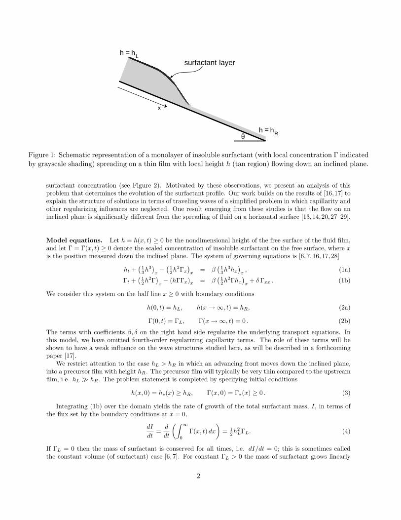
The dynamics of thin liquid films on solid substrates have been studied extensively in a variety of contexts,including gravity-driven flows [4, 12, 22, 31], spin-coating [30], and flows driven by strong surface tension[1, 25, 26]. Under lubrication theory, the governing equations for free-surface Stokes flow of thin films ofviscous fluids can be reduced to a single nonlinear evolution equation for the surface height, h = h(x, t)[26]. When surface tension is significant, the equation is fourth-order. Marangoni surface stresses aredriving forces created by variations in the coefficient of surface tension. These forces can be generatedby thermal [2, 23], electrical [19], or chemical means [20]. Flows driven by Marangoni stresses have beenfound to yield interesting instabilities and new kinds of waves [2, 5, 14, 21]. Chemical Marangoni stressescan be generated by the presence of surfactants (surface active agents), which typically decrease surfacetension; nonuniform distributions of surfactant molecules creates such surface stresses [3, 13, 14]. Insolublesurfactants are transported by the fluid flow at the free surface, leading to a coupled PDE system for theconcentration of surfactant and the film height [3, 9, 27–29] (see Figure 1).

In a series of recent numerical studies, Edmonstone, Matar, and Craster [6,7] considered one-dimensionalflow with surfactant down an inclined plane, and explored the stability to transverse perturbations. Aninteresting observation arising from their study is that when surfactant is supplied from an upstreamreservoir, it accumulates at the leading edge of the flow, resulting in a steady increase of the maximum

∗Dept. of Mathematics and Center for Nonlinear and Complex Systems, Duke University, Durham NC 27708-0320. Researchsupported by NSF Grants DMS-0239125 CAREER and DMS-0244498 FRG.

†Dept. of Mathematics and Center for Research in Scientific Computation, N.C. State University Raleigh, NC 27695. AdjunctProfessor, Dept. of Mathematics, Duke University. Research supported by NSF grant DMS-0244491 FRG.

‡Dept. of Mathematics, Duke University, Durham NC 27708. Research supported by NSF Grants DMS-0239125 CAREERand DMS-0244498 FRG.

1

x

hh L

hRθ

surfactant layer=

h =

Figure 1: Schematic representation of a monolayer of insoluble surfactant (with local concentration Γ indicatedby grayscale shading) spreading on a thin film with local height h (tan region) flowing down an inclined plane.

surfactant concentration (see Figure 2). Motivated by these observations, we present an analysis of thisproblem that determines the evolution of the surfactant profile. Our work builds on the results of [16,17] toexplain the structure of solutions in terms of traveling waves of a simplified problem in which capillarity andother regularizing influences are neglected. One result emerging from these studies is that the flow on aninclined plane is significantly different from the spreading of fluid on a horizontal surface [13,14,20,27–29].

Model equations. Let h = h(x, t) ≥ 0 be the nondimensional height of the free surface of the fluid film,and let Γ = Γ(x, t) ≥ 0 denote the scaled concentration of insoluble surfactant on the free surface, where xis the position measured down the inclined plane. The system of governing equations is [6, 7, 16,17,28]

ht +(

13h3

)x− (

12h2Γx

)x

= β(

13h3hx

)x

, (1a)

Γt +(

12h2Γ

)x− (hΓΓx)x = β

(12h2Γhx

)x

+ δ Γxx . (1b)

We consider this system on the half line x ≥ 0 with boundary conditions

h(0, t) = hL, h(x →∞, t) = hR, (2a)

Γ(0, t) = ΓL, Γ(x →∞, t) = 0 . (2b)

The terms with coefficients β, δ on the right hand side regularize the underlying transport equations. Inthis model, we have omitted fourth-order regularizing capillarity terms. The role of these terms will beshown to have a weak influence on the wave structures studied here, as will be described in a forthcomingpaper [17].

We restrict attention to the case hL > hR in which an advancing front moves down the inclined plane,into a precursor film with height hR. The precursor film will typically be very thin compared to the upstreamfilm, i.e. hL À hR. The problem statement is completed by specifying initial conditions

h(x, 0) = h∗(x) ≥ hR, Γ(x, 0) = Γ∗(x) ≥ 0 . (3)

Integrating (1b) over the domain yields the rate of growth of the total surfactant mass, I, in terms ofthe flux set by the boundary conditions at x = 0,

dI

dt=

d

dt

(∫ ∞

0

Γ(x, t) dx

)= 1

2h2LΓL. (4)

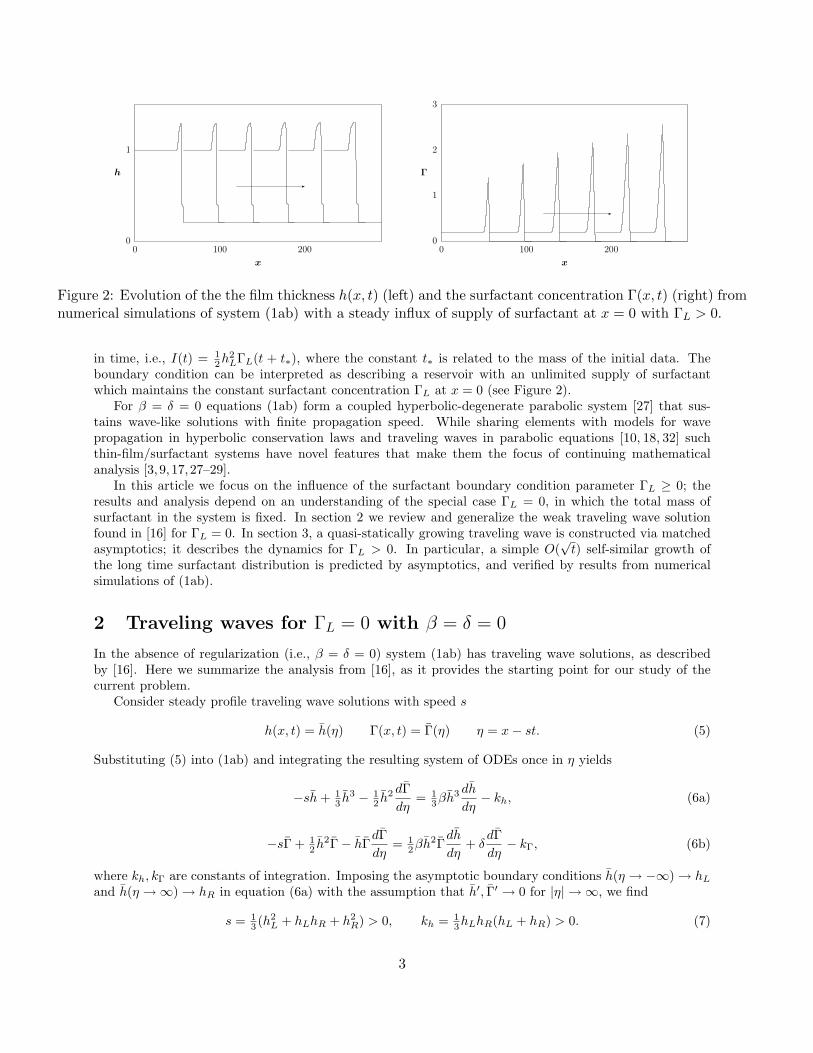
If ΓL = 0 then the mass of surfactant is conserved for all times, i.e. dI/dt = 0; this is sometimes calledthe constant volume (of surfactant) case [6, 7]. For constant ΓL > 0 the mass of surfactant grows linearly

2

0

1

0 100 200

h

x

0

1

2

3

0 100 200

Γ

x

Figure 2: Evolution of the the film thickness h(x, t) (left) and the surfactant concentration Γ(x, t) (right) fromnumerical simulations of system (1ab) with a steady influx of supply of surfactant at x = 0 with ΓL > 0.

in time, i.e., I(t) = 12h2

LΓL(t + t∗), where the constant t∗ is related to the mass of the initial data. Theboundary condition can be interpreted as describing a reservoir with an unlimited supply of surfactantwhich maintains the constant surfactant concentration ΓL at x = 0 (see Figure 2).

For β = δ = 0 equations (1ab) form a coupled hyperbolic-degenerate parabolic system [27] that sus-tains wave-like solutions with finite propagation speed. While sharing elements with models for wavepropagation in hyperbolic conservation laws and traveling waves in parabolic equations [10, 18, 32] suchthin-film/surfactant systems have novel features that make them the focus of continuing mathematicalanalysis [3, 9, 17,27–29].

In this article we focus on the influence of the surfactant boundary condition parameter ΓL ≥ 0; theresults and analysis depend on an understanding of the special case ΓL = 0, in which the total mass ofsurfactant in the system is fixed. In section 2 we review and generalize the weak traveling wave solutionfound in [16] for ΓL = 0. In section 3, a quasi-statically growing traveling wave is constructed via matchedasymptotics; it describes the dynamics for ΓL > 0. In particular, a simple O(

√t) self-similar growth of

the long time surfactant distribution is predicted by asymptotics, and verified by results from numericalsimulations of (1ab).

2 Traveling waves for ΓL = 0 with β = δ = 0

In the absence of regularization (i.e., β = δ = 0) system (1ab) has traveling wave solutions, as describedby [16]. Here we summarize the analysis from [16], as it provides the starting point for our study of thecurrent problem.

Consider steady profile traveling wave solutions with speed s

h(x, t) = h(η) Γ(x, t) = Γ(η) η = x− st. (5)

Substituting (5) into (1ab) and integrating the resulting system of ODEs once in η yields

−sh + 13 h3 − 1

2 h2 dΓdη

= 13βh3 dh

dη− kh, (6a)

−sΓ + 12 h2Γ− hΓ

dΓdη

= 12βh2Γ

dh

dη+ δ

dΓdη

− kΓ, (6b)

where kh, kΓ are constants of integration. Imposing the asymptotic boundary conditions h(η → −∞) → hL

and h(η →∞) → hR in equation (6a) with the assumption that h′, Γ′ → 0 for |η| → ∞, we find

s = 13 (h2

L + hLhR + h2R) > 0, kh = 1

3hLhR(hL + hR) > 0. (7)

3

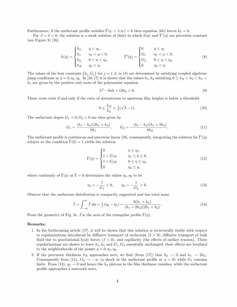
Furthermore, if the surfactant profile satisfies Γ(η → ±∞) = 0 then equation (6b) forces kΓ = 0.For β = δ = 0, the solution is a weak solution of (6ab) in which h(η) and Γ′(η) are piecewise constant

(see Figure 3) [16]:

h(η) =

hL η < η1,

h1 η1 < η < 0,

h2 0 < η < η2,

hR η2 < η,

Γ′(η) =

0 η < η1

G1 η1 < η < 0,

G2 0 < η < η2,

0 η2 < η.

(8)

The values of the four constants {hj , Gj} for j = 1, 2, in (8) are determined by satisfying coupled algebraicjump conditions at η = 0, η1, η2. In [16,17] it is shown that the values h1, h2 satisfying 0 ≤ hR < h2 < hL <h1 are given by the positive real roots of the polynomial equation

h3 − 6sh + 12kh = 0. (9)

These roots exist if and only if the ratio of downstream to upstream film heights is below a threshold:

0 ≤ hR

hL< 1

2 (√

3− 1). (10)

The surfactant slopes G1 > 0, G2 < 0 are then given by

G1 =(h1 − h2)(2h1 + h2)

6h1, G2 = − (h1 − h2)(h1 + 2h2)

6h2. (11)

The surfactant profile is continuous and piecewise linear [16], consequently, integrating the solution for Γ′(η)subject to the condition Γ(0) = 1 yields the solution

Γ(η) =

0 η ≤ η1,

1 + G1η η1 ≤ η ≤ 0,

1 + G2η 0 ≤ η ≤ η2,

0 η2 ≤ η,

(12)

where continuity of Γ(η) at Γ = 0 determines the values η1, η2 to be

η1 = − 1G1

< 0, η2 = − 1G2

> 0. (13)

Observe that the surfactant distribution is compactly supported and has total mass

I =∫ ∞

−∞Γ dη = 1

2 (η2 − η1) =6(h1 + h2)

(h1 + 2h2)(2h1 + h2). (14)

From the geometry of Fig. 3c, I is the area of the triangular profile Γ(η).

Remarks:

1. In the forthcoming article [17], it will be shown that this solution is structurally stable with respectto regularizations introduced by diffusive transport of surfactant (δ > 0), diffusive transport of bulkfluid due to gravitational body forces (β > 0), and capillarity (the effects of surface tension). Theseregularizations are shown to leave h1, h2 and G1, G2 essentially unchanged; their effects are localizedto the neighborhoods of the points η = 0, η1, η2.

2. If the precursor thickness hR approaches zero, we find (from [17]) that h2 → 0 and h1 → 2hL.Consequently from (11), G2 → −∞ (a shock in the surfactant profile at η = 0) while G1 remainsfinite. From (13), η2 → 0 and hence the h2 plateau in the film thickness vanishes, while the surfactantprofile approaches a sawtooth wave.

4

(a)

hR

h2

h1

hL

η

h

η20η1

1

0

(b)

G2

G1

η

Γ′

η20η1

0

−1

(c)

Γ′= G2

Γ′= G1

η

Γ

η20η1

1

0

Figure 3: The weak traveling solution, (8): (a) the piecewise constant h(η) profile, (b) the piecewise constantΓ′(η) profile, and (c) the piecewise linear profile for Γ(η), (12). For imposed boundary conditions hL = 1 andhR = 0.1, equations (9), (11) and (13) yield the values h1 ≈ 1.3787, h2 ≈ 0.2019, G1 ≈ 0.4210, G2 ≈ −1.7316,η1 ≈ −2.3753, η2 ≈ 0.5775.

5

2.1 Scale-invariant structure of the traveling wave

The condition Γ(0) = 1 determining the maximum surfactant concentration is an arbitrary normalization.This condition can be imposed at η = 0 thanks to translation invariance of the PDEs (1ab). The maximumvalue itself can be set to any positive constant, Γmax ≡ m > 0. In [16] it was noted that the solutions of(1ab) with β = δ = 0 are invariant under the continuous one-parameter scaling h → h, Γ → mΓ, x → x/m,t → t/m. Consequently, up to translation invariance, the general traveling wave solution of (1ab) withβ = δ = 0 subject to boundary conditions (2ab) with ΓL = 0 is

h(x, t) = h

(x− st

m

), Γ(x, t) = m Γ

(x− st

m

), (15)

for any m > 0.Note that the trivial case of no surfactant (Γ ≡ 0) corresponds to the singular case of (15) with m = 0,

h0(η) =

{hL η < 0,

hR 0 < η,Γ0(η) ≡ 0. (16)

The wave speed given by (7) is independent of m ≥ 0. For m = 0, this is to be expected from the factthat (16) is the shock wave solution of the decoupled equation ht +

(13h3

)x

= 0, a scalar conservation law.We can therefore interpret the influence of the surfactant as modifying the shape of the surfactant-freeshock profile (16), effectively broadening the width of the shock structure through the introduction of theh1 and h2 plateau regions. In the limit of vanishing surfactant concentration, Γmax → 0, we observe thatη2 − η1 → 0, so although h1, h2 are independent of Γmax, solution (15) collapses to solution (16), shrinkingthe plateau with height h1 to zero width.

It is noteworthy that solution (15) depends upon having upstream and downstream film heights belowthe critical ratio (10). If 1

2 (√

3− 1) < hR/hL < 1, then a different solution emerges from PDE simulations,even though the surfactant-free solution is still a single monotonic traveling wave. The structure of the newsolution is the subject of current investigation.

3 Dynamics for ΓL > 0 with β, δ > 0

We now focus on understanding the role of the boundary condition parameter ΓL in determining thedynamics, as in the simulation with ΓL > 0 shown in Figure 2.

If ΓL = 0 then the total amount of surfactant is conserved for all times. If β = δ = 0 and we have atraveling wave solution (15) for the surfactant profile, then the value of m is determined by the mass of theinitial condition Γ∗(x) (3),

I =∫ ∞

0

Γ∗(x) dx = m2

∫Γ(ζ) dζ = m2I , (17)

with I given by (14). More generally, we expect that the traveling wave solution (15) is structurally stableand attracting for t →∞ from a broader set of initial data and small positive β, δ.

If ΓL > 0 then there are no smooth bounded traveling wave solutions of (6ab) satisfying upstreamand downstream boundary conditions. To see this, we note that the upstream condition implies kΓ =( 12h2

L − s)ΓL, whereas the downstream boundary condition gives kΓ = 0. For ΓL > 0 these are consistentonly in the special case s = 1

2h2L; from (7), this yields the condition hR/hL = 1

2 (√

3−1), the threshold valuefrom (10). This leads to the trivial solution h = constant as the only bounded traveling wave at this speed.But this solution conflicts with the boundary conditions, hL > hR, so it is not acceptable. Consequently,the solution of (1ab) in this case must take a different form; we will turn to the use of matched asymptoticsto construct the solution.

The behavior observed in numerical simulations in Figure 2 suggests that the solution with ΓL > 0 stillresembles the traveling wave solution (15). However, the Γ profile evolves, suggesting that the maximumof Γ should be generalized to be a time-dependent increasing function, m(t), to be used in (15). We nowpresent analysis to support this description.

6

0

1

-80 -40 0 40

h

x − x0(t)

0

10

20

30

-80 -40 0 40

Γ

x − x0(t)

Figure 4: Long-time evolution of the the film thickness h(x, t) (left) and the surfactant concentration Γ(x, t)(right) from numerical simulations of system (1ab) with hL = 1, hR = 0.1, β = 0.1, δ = 0.01, and ΓL = 0.2.Time profiles for t = 5000, 10000, 15000, . . . , 60000 shifted into the reference frame x−x0(t) where the positionof the maximum of Γ(x, t) is stationary.

0

1

η1 0 η2

h∼

h

(x − x0(t))/Γmax(t)

1

η1 0

1

η1 0 η2

Γ(x

,t)

/Γ

max(t

)

(x − x0(t))/Γmax(t)

0η1

Figure 5: The long-time solution profiles from Figure 4 rescaled according to (18). Dashed lines show thetraveling wave solution (8), (12). Insets show details of the evolution near η1 ≈ −2.375, given by (13).

3.1 Approximate global solution for t →∞Motivated by the above discussion, we consider a change of variables that allows for time-dependence inthe maximum of Γ and in the speed of propagation. All solutions of (1ab) can be written in the form

h(x, t) = h(ζ, t) Γ(x, t) = m(t) Γ(ζ, t), ζ =x− x0(t)

m(t). (18)

where the functions x0(t), m(t) must be determined. Substituting (18) into (1ab) yields the new governingPDEs

ht − x′0(t)hζ −m′(t)ζhζ +(

13 h3

)ζ−

(12 h2Γζ

)ζ

=β

m(t)

(13 h3hζ

)ζ

, (19a)

Γt − x′0(t)Γζ −m′(t)ζΓζ + m′(t)Γ +(

12 h2Γ

)ζ−

(hΓΓζ

)ζ

=β

m(t)

(12 h2Γhζ

)ζ

+δ

m(t)Γζζ . (19b)

For concreteness, in numerical simulations, x0(t) will be defined by the position of the maximum of Γ(x, t).Figure 4 shows that in this moving reference frame, h, Γ exhibit a well-defined growth. To depict thescaled forms h and Γ, the same profiles are plotted in the forms (18) in Figure 5 with m(t) replaced by thenumerical result Γmax(t) = maxx Γ(x, t).

Plotted in this form, the profiles indeed appear to approach the traveling wave solution, (8) and (12),as t →∞. This behavior can be obtained directly from (19ab) subject to the assumptions:

7

1. As t → ∞ the rescaled solutions h, Γ converge to quasi-steady profiles that are independent of t:h → h(ζ), Γ → Γ(ζ).

2. The maximum of the surfactant profile grows slowly (sub-linearly) with time,

m(t) = O(tα), as t →∞ with 0 < α < 1. (20)

3. The propagation speed x′0(t) remains bounded for all times and approaches a positive constant:x′0(t) → s > 0, as t →∞.

Assumption 1, supported by Figure 5, suggests that the ht, Γt terms in (19ab) can be neglected to yieldequations involving only ζ-derivatives of h, Γ. From assumption 2, m(t) → ∞ and m′(t) → 0 as t → ∞.Consequently the terms on the right hand sides of (19ab) will vanish since β/m → 0 and δ/m → 0. Thusregularization offered by these terms becomes negligible for long times. Similarly the terms on the left sidesmultiplied by m′(t) become negligible (with the mild assumption that ζhζ , ζΓζ are bounded as |ζ| → ∞).Using assumption 3, the resulting equations for t →∞ can be integrated once in ζ to yield

−sh + 13 h3 − 1

2 h2 dΓdζ

= −kh , (21a)

−sΓ + 12 h2Γ− hΓ

dΓdζ

= −kΓ , (21b)

where kh, kΓ are constants of integration. Suitable boundary conditions corresponding to (2a), (2b) aregiven by

h(ζ → −∞) = hL, h(ζ →∞) = hR , (21c)

Γ(ζ → −∞) = 0, Γ(ζ →∞) = 0 . (21d)

The boundary condition on Γ(ζ → −∞) follows from Γ(ζ → ∞) = ΓL/m(t) → 0 as t → ∞. As a result,the influence of the boundary condition ΓL does not enter in the leading order problem (21ab) for t →∞.At this point we observe that problem (21ab) reduces to that of section 2 (6ab) and we have the leadingorder solution for t →∞,

h(ζ, t) ∼ h(ζ), Γ(ζ, t) ∼ Γ(ζ), x′0(t) ∼ s. (22)

Returning to the original PDE system (1ab) on the domain x > 0, assumption 2 is justified by consideringthe evolution of the mass of surfactant. Figure 2 suggests that the surfactant profile with ΓL > 0 can beapproximated by a uniform layer with Γ = ΓL together with a growing triangular profile (12), scaled as in(15) by m(t). With respect to calculating the mass of surfactant, this approximate description of Γ(x, t)can be expected to yield a vanishingly small relative error as t →∞. Hence for long times, I(t) is given by

I(t) =∫ ∞

0

Γ dx ≈ ΓLs(t + t0) + 12Γ2

L|η1|+ m2(t)∫ η2

η1

Γ(η) dη , (23)

where t0 is a constant related to initial conditions. The first term on the right of (23) is the surfactantin the uniform ΓL layer with length increasing at a rate equal to the propagation speed of the advancingtriangular wave (asymptotically x′0 ∼ s). The second term is a finite contribution from the region joiningthe uniform layer to the triangular profile. Substituting (23) into (4) yields

dI

dt≈ I

d(m2)dt

+ sΓL = 12h2

LΓL. (24)

Using (7), we obtain

m(t) ∼(

ΓL

6I(h2

L − 2hLhR − 2h2R)

)1/2√t + t∗ t →∞. (25)

8

m(t)Γmax(t)

t

6000040000200000

30

20

10

0

Figure 6: Comparison of the maximum surfactant concentration from the numerical simulation of Figs. 4,5,Γmax(t) = maxx Γ(x, t) (solid dots) and the predicted evolution m(t) given by (25) (solid curve).

Consequently, the second assumption, (20), is verified with α = 12 .1 Observe that the condition that the

coefficient of (25) be real requires that 1 − 2r − 2r2 > 0 where r is the ratio r = hR/hL. The resultingcondition on this ratio is 0 < r < 1

2 (√

3− 1), precisely coinciding with the condition (10) for the existenceof steady profile waves [16]. Figure 6 shows excellent agreement between the prediction (25) and the resultsof the numerical simulations.

In summary, we have shown that for long times, the solutions approach growing traveling waves,

h(x, t) ∼ h

(x− x0(t)

m(t)

), Γ(x, t) ∼ m(t) Γ

(x− x0(t)

m(t)

). (26)

Some further comments are appropriate at this point. First, for large times, when the influence of theboundary conditions at x = 0 are weak, the traveling wave solutions of (1ab) should be invariant withrespect to spatial translations, x → x + ε1 for any real ε1. But secondly, from the autonomous equations(21ab), the long time growing solutions (18) should also be invariant with respect to translations in theirspatial variable, ζ → ζ + ε2 for some ε2. Combining these observations, we note that the general form forthe moving reference frame for t →∞ is

x0(t) ∼ st− ε2m(t)− ε1, =⇒ dx0

dt∼ s− ε2m

′(t) ∼ s. (27)

This validates the third assumption. See Figure 7(left) for numerical evidence supporting (27). If x0(t) isknown, then from (18) the positions defining the region of support of the dominant distribution (η1, η2) aregiven by

x1(t) = x0(t) + η1m(t), x2(t) = x0(t) + η2m(t), (28)

see Figure 7(right).One final remaining issue is that while that (26) suggests that Γ(x, t) = 0 for x < x1(t), it is clear from

Figure 2 that Γ ∼ ΓL > 0. This is resolved in the next subsection via boundary layer analysis.

3.2 Boundary layer structures at the jump discontinuities η1 and η2

The limit 1/m → 0 in (19ab) eliminated the regularization given by the second-order terms on the right-hand sides of those equations. This is a singular perturbation [11, 15] of the full system for t → ∞ andhence the weak solution (26) should be interpreted as a leading order outer solution. In particular, it is

1Note that the traveling wave solution (22) could also be expected for time-dependent boundary conditions, ΓL(t) = O(tγ) if0 ≤ γ < 1. For γ = 1, the m′(t) terms on the left sides of (19ab) must be retained, which would lead to a new class of self-similarsolutions.

9

t

x0(t

)−

st

800006000040000200000

120

110

100

90

80

x1(t) − x0(t)

x2(t) − x0(t)

t

x−

x0(t

)

800006000040000200000

40

0

-40

-80

Figure 7: (Left) Position of the moving reference frame relative to the asymptotic traveling wave speed s = 0.37from (7): values from the numerical simulation (solid dots) show a O(c1 + c2

√t) lag (solid curve) as predicted

by (27). (Right) Positions of the edges of the region of support of the triangular surfactant profile relativeto x0(t): numerical simulation values (dots) compared with prediction (28) (solid curves) with η1 ≈ −2.375,η2 ≈ 0.5775, given by (13), and m(t) ≈ 0.1327

√t + t∗ from (25) for hL = 1, hR = 0.1 and ΓL = 0.2.

not uniformly valid for all ζ; at points where jump discontinuities occur in h(ζ), Γ(ζ) the influence of thehigher-order terms may strongly influence the local structure of the solution, see insets in Figure 5. In thissubsection, we use matched asymptotics to construct boundary layer solutions as inner expansions of thesolution in the neighborhoods of the shocks at η1 and η2. These inner solutions can be combined with (26)and a boundary layer at η = 0 (considered in section 3.3) to yield a uniformly valid approximate solution.

Define ε ≡ 1/m → 0 as a small parameter for the limit t → ∞. Consider a small neighborhood ofthe shock at ζ = η1, defined by ζ = η1 + ελy with λ > 0 to be determined and y = O(1). The profile h

remains finite and bounded, so the quasi-steady solution should take the form h = h(y) + O(ε). Similarlywe expect that for ζ ≤ η1 the scaled surfactant is of the order Γ ≈ ΓL/m = O(ε), hence the solution shouldbe Γ = εΓ(y) + O(ε2). Substituting these into (19ab) and balancing the dominant terms determines thescaling to be λ = 1 and (after integrating in y) yields the leading order equations

− [s1 + η1m′(t)] h + 1

3 h3 − 12 h2 dΓ

dy= 1

3βh3 dh

dy− kh,1, (29a)

− [s1 + η1m′(t)] Γ + 1

2 h2Γ− hΓdΓdy

= 12βh2Γ

dh

dy+ δ

dΓdy

− kΓ,1, (29b)

where the k’s are constants and we have removed the assumption from (22) that the speed s1 is known.Note that the m′(t) terms are formally higher order terms as t →∞, but we retain them in (29ab) to helpindicate the fact that the boundary layer solution is slowly varying in time and has speed different from x′0(t)(see (28)). Neglecting this weak variation, observe that (29ab) take the same form as the traveling waveequations (6ab). Hence the boundary layer solution is also a traveling wave, see Figure 8. One differencehowever, is that the solutions of (29ab) are subject to only the left boundary conditions h(y → −∞) → hL,Γ(y → −∞) → ΓL which determine the constants of integration for t →∞ to be

kh,1 = s1hL − 13h3

L, kΓ,1 = s1ΓL + 12h2

LΓL. (29c)

In contrast to (7), note that the speed s1 has not yet been determined.An analogous set of boundary layer equations can be obtained in the neighborhood of η2 with η1 replaced

by η2 and different constants for kh,2 and kΓ,2, s2 determined by the boundary conditions h(y →∞) → hR,Γ(y →∞) → 0,

kh,2 = s2hR − 13h3

R, kΓ,2 = 0. (30)

The traveling wave structure of these solutions are shown in Figure 9. The need for this boundary layeris not as apparent as for (29abc) since the outer solution (26) is compatible with the boundary conditions

10

0

1

-20 0 20 40

h

y ∼ x − x1(t)

0

4

8

12

-20 0 20 40

Γ

y ∼ x − x1(t)

Figure 8: The numerical solution profiles from Figure 5 shifted into the reference frame for the boundarylayer at η1 where locally (here roughly y < 20), the solution is a quasi-steady traveling wave, stationary inthis frame (boxed). The outer solution spreads to the right in this reference frame.

0

1

-40 -20 0

h

y ∼ x − x2(t)

0

4

8

12

-40 -20 0

Γ

y ∼ x − x2(t)

Figure 9: The numerical solution profiles from Figure 5 shifted into the reference frame for the boundarylayer at η2 where locally (here roughly −5 < y), the solution is a quasi-steady traveling wave, stationary inthis frame (boxed). The outer solution spreads to the left in this reference frame.

for y → ∞. However, like the solution at η1, this solution at η2 gives the structure defining the smoothtransition from one level of h to another, h2 → hR (hL → h1 at η1), and from one slope of Γ to another,Γ′ = G2 → Γ′ = 0 (Γ′ = 0 → Γ′ = G1 at η1).

With respect to system (19ab) the inner solutions exhibit sharpening features with the widths of theboundary layers decreasing as t → ∞ (see insets in Figure 5). However under the rescaling appropriateto the boundary layers, we observe that these solutions are quasi-steady traveling waves. Moreover, theboundary layer scaling essentially returns the system to the original form (1ab) with y ∼ x, h ∼ h, andΓ ∼ Γ. Consequently, while for ΓL > 0 the solution is not globally a traveling wave, traveling wave solutionsstill accurately describe h,Γ locally in these boundary layers (see Figures 8, 9).

3.3 Boundary layer at η = 0

As described above, on the ζ = O(1) lengthscale, for m →∞, the solution approaches (22) and appears tohave jump discontinuities in h, Γ′ at ζ = 0. Like the behavior at η = η1, η2, the presence of higher-orderregularization smooths the solution over a narrow boundary layer at ζ = 0. However, the structure at η = 0is different than in the other boundary layers because here Γ = O(m) →∞ whereas Γ = O(1) near η1, η2.

To characterize the boundary layer at η = 0, where Γ reaches it’s maximum, m(t) = Γmax(t), we usethe ansatz

h(x, t) ∼ h(η) Γ(x, t) ∼ m(t) + Γ(η) η = x− st, (31)

11

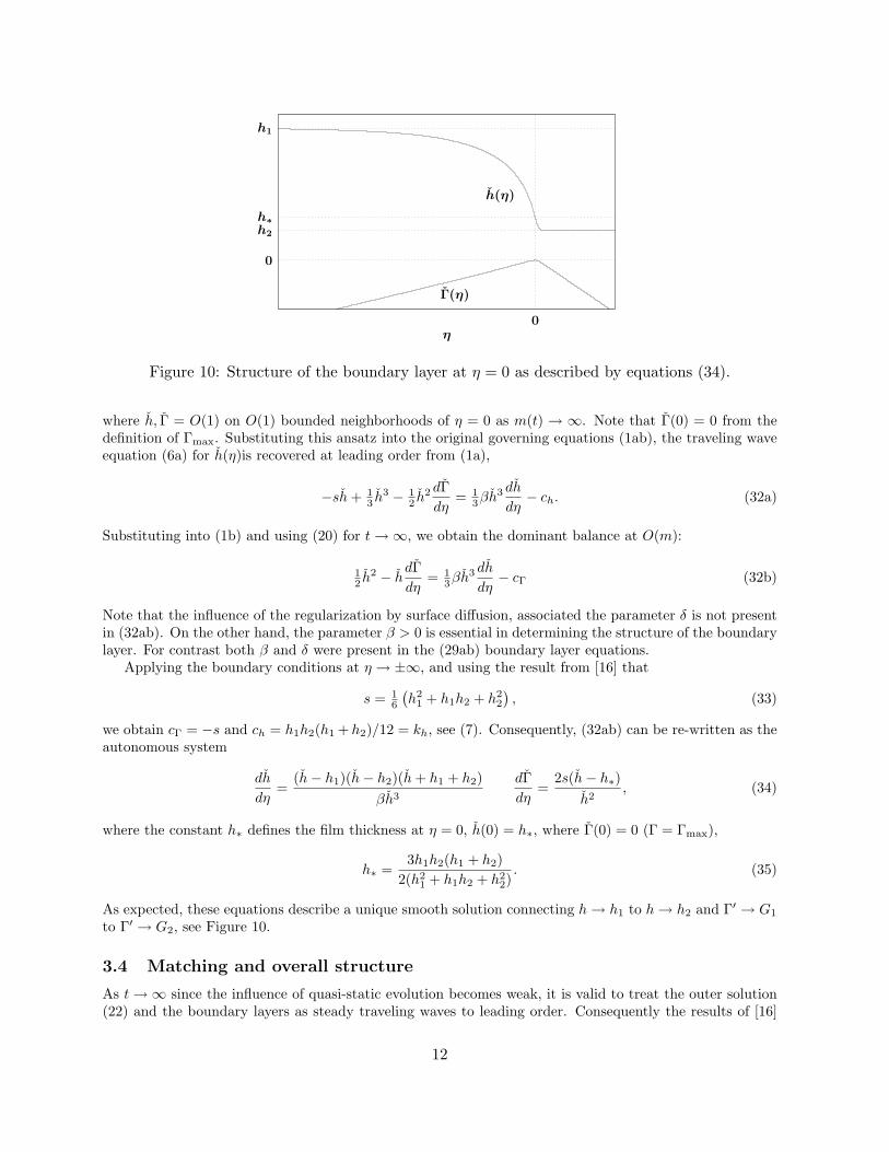
Γ(η)

h(η)

η0

h1

h∗

h2

0

Figure 10: Structure of the boundary layer at η = 0 as described by equations (34).

where h, Γ = O(1) on O(1) bounded neighborhoods of η = 0 as m(t) → ∞. Note that Γ(0) = 0 from thedefinition of Γmax. Substituting this ansatz into the original governing equations (1ab), the traveling waveequation (6a) for h(η)is recovered at leading order from (1a),

−sh + 13 h3 − 1

2 h2 dΓdη

= 13βh3 dh

dη− ch. (32a)

Substituting into (1b) and using (20) for t →∞, we obtain the dominant balance at O(m):

12 h2 − h

dΓdη

= 13βh3 dh

dη− cΓ (32b)

Note that the influence of the regularization by surface diffusion, associated the parameter δ is not presentin (32ab). On the other hand, the parameter β > 0 is essential in determining the structure of the boundarylayer. For contrast both β and δ were present in the (29ab) boundary layer equations.

Applying the boundary conditions at η → ±∞, and using the result from [16] that

s = 16

(h2

1 + h1h2 + h22

), (33)

we obtain cΓ = −s and ch = h1h2(h1 + h2)/12 = kh, see (7). Consequently, (32ab) can be re-written as theautonomous system

dh

dη=

(h− h1)(h− h2)(h + h1 + h2)βh3

dΓdη

=2s(h− h∗)

h2, (34)

where the constant h∗ defines the film thickness at η = 0, h(0) = h∗, where Γ(0) = 0 (Γ = Γmax),

h∗ =3h1h2(h1 + h2)

2(h21 + h1h2 + h2

2). (35)

As expected, these equations describe a unique smooth solution connecting h → h1 to h → h2 and Γ′ → G1

to Γ′ → G2, see Figure 10.

3.4 Matching and overall structure

As t →∞ since the influence of quasi-static evolution becomes weak, it is valid to treat the outer solution(22) and the boundary layers as steady traveling waves to leading order. Consequently the results of [16]

12

may be applied directly to carry out the asymptotic matching of the boundary layers to the outer solution.Notably, it is found that the leading order wave speeds are identical,

s = s1 = s2, (36)

for s given by (7). Briefly, matching the boundary layer at η1 to the outer solution (26) requires finding asolution of (29ab) that satisfies h(y →∞) → h1 and Γ(y →∞) →∞ with Γ′(y →∞) → G1. Substitutingthese into (29b) yields −s1 + 1

2h21 − h1G1 = 0, similar to [16]. It is notable that this algebraic matching

condition, and likewise the one obtained from (29a) are independent of ΓL. The consequence is that toleading order for long times, despite the fact that the outer solution is a self-similar growing profile (26),the overall solution (outer and boundary layers) can be understood in terms of a single traveling wave withspeed s.

4 Discussion and conclusions

The presence of a finite mass of insoluble surfactant on a film moving down an inclined substrate introducesnew structure to the leading edge of the fluid film. Provided that the threshold condition (10) holds, despitethe new structure of the film, the solution propagates with the same speed as if there were no surfactant.

When surfactant is continually supplied from upstream, the solution is is no longer a traveling wave.While a well-defined wave speed is maintained, in the frame of reference moving with that speed, thesolution exhibits a self-similar growing form for t → ∞; similar behavior has been observed in other thinfilm problems [8, 24]. We have been able to obtain expressions for the accumulation of surfactant andleading order asymptotic forms for the film and surfactant profiles subject to relatively few assumptionson the dynamics. While the arguments presented here are not rigorous, the approaches considered couldprovide good starting points for further analyses of this problem.

In forthcoming work [17], further analysis of the traveling wave (8) will be presented: structural stabilitywith respect to regularization and the limits of β → 0, δ → 0 and weak fourth-order capillary effects, aswell as other questions of stability. It is worth noting again that the solutions presented here depend on thethreshold condition (10). Above this threshold, for example in the case of an initially flat film, the form ofsolutions is not known, and numerical simulations suggest that more complicated dynamics take place [16].Further work on this problem is being pursued [17].

Acknowledgments

We thank the referee for incisive questions and helpful suggestions that improved the article. Parts of thisresearch were presented by MS at the IPAM workshop on Thin Films and Fluid Interfaces. We thank theorganizers and IPAM for an enjoyable and productive meeting.

References

[1] A. L. Bertozzi. The mathematics of moving contact lines in thin liquid films. Notices Amer. Math.Soc., 45(6):689–697, 1998.

[2] A. L. Bertozzi, A. Munch, and M. Shearer. Undercompressive shocks in thin film flows. Physica D,134(4):431–464, 1999.

[3] M. S. Borgas and J. B. Grotberg. Monolayer flow on a thin film. J. Fluid Mech., 193:151–170, 1988.

[4] J. Buckmaster. Viscous sheets advancing over dry beds. Journal of Fluid Mechanics, 81:735–756, 1977.

[5] A. D. Dussaud, O. K. Matar, and S. M. Troian. Interfacial profile and spreading rate of a surfactantfilm advancing on a thin liquid layer: Comparison between theory and experiment. J. Fluid Mech.,544:23–51, 2005.

13

[6] B. D. Edmonstone, O. K. Matar, and R. V. Craster. Flow of surfactant-laden thin films down aninclined plane. J. Engrg. Math., 50(2-3):141–156, 2004.

[7] B. D. Edmonstone, O. K. Matar, and R. V. Craster. Surfactant-induced fingering phenomena in thinfilm flow down an inclined plane. Phys. D, 209(1-4):62–79, 2005.

[8] J. C. Flitton and J. R. King. Surface-tension-driven dewetting of Newtonian and power-law fluids. J.Engrg. Math., 50(2-3):241–266, 2004.

[9] H. Garcke and S. Wieland. Surfactant spreading on thin viscous films: Nonnegative solutions of acoupled degenerate system. SIAM Journal on Mathematical Analysis, 37(6):2025–2048, 2006.

[10] B. H. Gilding and R. Kersner. Travelling waves in nonlinear diffusion-convection reaction. Progressin Nonlinear Differential Equations and their Applications, 60. Birkhauser Verlag, Basel, 2004.

[11] M. H. Holmes. Introduction to perturbation methods, volume 20 of Texts in Applied Mathematics.Springer-Verlag, New York, 1995.

[12] H. Huppert. Flow and instability of a viscous current down a slope. Nature, 300:427–429, 1982.

[13] O. E. Jensen and J. B. Grotberg. Insoluble surfactant spreading on a thin viscous film: shock evolutionand film rupture. J. Fluid Mech., 240:259–288, 1992.

[14] O. E. Jensen and J. B. Grotberg. The spreading of heat or soluble surfactant along a thin liquid film.Physics of Fluids A, 5(1):58–68, 1993.

[15] J. Kevorkian and J. D. Cole. Multiple scale and singular perturbation methods, volume 114 of AppliedMathematical Sciences. Springer-Verlag, New York, 1996.

[16] R. Levy and M. Shearer. The motion of a thin film driven by surfactant and gravity. SIAM Journalof Applied Mathematics, 66(5):1588–1609, 2006.

[17] R. Levy, M. Shearer, and T. P. Witelski. Structure of traveling waves in a thin film-surfactant system.in preparation, 2006.

[18] J. D. Logan. Transport modeling in hydrogeochemical systems, volume 15 of Interdisciplinary AppliedMathematics. Springer-Verlag, New York, 2001.

[19] H.-W. Lu, K. Glasner, A. L. Bertozzi, and C.-J. Kim. A diffuse interface model for electrowettingdroplets in a hele-shaw cell. J. Fluid Mech., submitted, 2005.

[20] O. K. Matar and S. M. Troian. Growth of non-modal transient structures during the spreading ofsurfactant coated films. Phys. Fluids, 10(5):1234–1236, 1998.

[21] O. K. Matar and S. M. Troian. The development of transient fingering patterns during the spreadingof surfactant coated films. Phys. Fluids, 11:3232–3246, 1999.

[22] J. A. Moriarty, L. W. Schwartz, and E. O. Tuck. Unsteady spreading of thin liquid films with smallsurface tension. Physics of Fluids A, 3(5):733–742, 1991.

[23] A. Munch. Pinch-off transition in Marangoni-driven thin films. Phys. Rev. Lett., 91(1):016105, 2003.

[24] A. Munch, B. A. Wagner, and T. P. Witelski. Lubrication models with small to large slip lengths.Journal of Engineering Mathematics, 53(3-4):359–383, 2005.

[25] T. G. Myers. Thin films with high surface tension. SIAM Rev., 40(3):441–462, 1998.

[26] A. Oron, S. H. Davis, and S. G. Bankoff. Long-scale evolution of thin liquid films. Reviews of ModernPhysics, 69(3):931–980, 1997.

[27] M. Renardy. On an equation describing the spreading of surfactants on thin films. Nonlinear Anal.,26(7):1207–1219, 1996.

[28] M. Renardy. A singularly perturbed problem related to surfactant spreading on thin films. NonlinearAnal., 27(3):287–296, 1996.

[29] M. Renardy. A degenerate parabolic-hyperbolic system modeling the spreading of surfactants. SIAMJ. Math. Anal., 28(5):1048–1063, 1997.

14

[30] L. W. Schwartz and R. V. Roy. Theoretical and numerical results for spin coating of viscous liquids.Phys. Fluids, 16(3):569–584, 2004.

[31] E. O. Tuck and L. W. Schwartz. A numerical and asymptotic study of some third-order ordinarydifferential equations relevant to draining and coating flows. SIAM Rev., 32(3):453–469, 1990.

[32] A. I. Volpert, V. A. Volpert, and V. A. Volpert. Traveling wave solutions of parabolic systems, volume140 of Translations of Mathematical Monographs. American Mathematical Society, Providence, RI,1994.

15