AAIT 2015 By: Nebiyou Kassahun I D N O GSR/2651/06 Groundwater potential assessment and characterization of Genale-Dawa River basin

Welcome message from author
This document is posted to help you gain knowledge. Please leave a comment to let me know what you think about it! Share it to your friends and learn new things together.
Transcript
[Type text]
AAIT
2015
By: Nebiyou Kassahun
I D N O G S R / 2 6 5 1 / 0 6
Groundwater potential assessment and characterization
of Genale-Dawa River basin
ADDIS ABABA UNIVERSITY SCHOOL OF GRADUATE STUDIES
FACULITY OF TECHNOLOGY
Groundwater potential Assesment and Character izat ion of Genale -Dawa river basin
A thesis submitted to the School of Graduate Studies of Addis Ababa University in partial fulfillment of the Degree of Masters of Science in Civil Engineering
(Stream: Hydraulic Engineering) By
Nebiyou kassahun
Approval by Board of Examiners
---------------------------------------------------- ------------------
Chairman (department of graduate committee) Signature
Dr.-Ing Mebruk Mohammed .
Advisor Signature
Dr. Agizew Nigussie . .
Internal Examiner Signature
Dr.-Ing. Asie Kemal Jabir .
External Examiner Signature


Groundwater potential assessment and characterization of Genale-Dawa River basin
By Nebiyou k. Page ii
Abstract
Genale-Dawa River Basin is one of the largest basins in Ethiopia. It is one of the most drought
prone regions in Ethiopia. As a result a search for alternative source of water has always been a
major issue in the region. This study therefore, aims at characterizing and evaluating the
ground water potential resource of Genale-Dawa basin. The results of this research ultimately
contribute to development of better water resources potential management.
Delineation of the Genale-Dawa River basin was carried out first in order to define the problem
domain of the model. This has resulted in 17860km2 area of the basin. This area was discretized
to form a three dimensional. The discretized region has 19620 nodes, 17862 equilateral
triangular elements of varying sizes with a maximum of 5km edge dimension and 2500km
model thickness.
The conceptualization of the model was done by grouping the discretized region in to 56
geological classes based on previous geological survey of the basin. The equivalent porous
medium modeling approach was used to represent the different geological classes in the basin.
Moreover, 23 rain gauge stations were used to determine the areal precipitation over the
basin. The model takes perennial rivers as constant head boundaries, the side and bottom
geometric boundaries of the model as no flow boundaries and the recharge due to
precipitation as specified flow boundary.
After conceptualization of the flow system was complete and numerical model developed,
TAGSAC model manual calibration was done by seating hydraulic conductivity and percentage
recharge as calibration parameters when calibration is complete. The result was evaluated
quantitatively using average indicators (AM, RMS, MAE) and qualitatively by comparison of
groundwater contour maps generated with recorded and simulated hydraulic head data.
The calibration model was then used to determine monthly groundwater table fluctuation
which eventually enabled the estimation of groundwater recharge potential of the basin.
Additionally, base flow separation of perennial rivers was done to determine the monthly
excess flux from the aquifer system. By adding these two values the total replenishable
groundwater was estimated to be 2.78BMC. Hydro-geological map was also prepared based on
hydraulic conductivity values obtained from model calibration. Identification of major
groundwater recharge and discharge areas have also been done as an attempt towards basic
groundwater flow system characterization.
Groundwater potential assessment and characterization of Genale-Dawa River basin
By Nebiyou k. Page iii
Key words:
Ethiopia; Genale Dawa River Basin; Numerical Groundwater modeling; Replenishable
Groundwater Potential; TAGSAC
Groundwater potential assessment and characterization of Genale-Dawa River basin
By Nebiyou k. Page iv
Acknowledgment
First, I would like thank Debremarkos University for granting me the scholarship to study in
Addis Ababa University and giving me a paid leave of absence during the time of my study and
research. Most of all, my greatest appreciation goes to my advisor, Dr. Mebruk Mohammed,
who invested his time, knowledge and energy throughout the whole research work. He is very
supportive, willing, and hard working; in generally he has been an inspiration to me
professionally. My deepest gratitude also goes to my family members who has encouraged me
and supported me in ideas to the completion of my work. Furthermore, I would also like to
express my warmest gratitude to Water Works Design and Supervision Enterprise, Ethiopian
Ministry of Water Resources and Energy, and National Metrological Agency for their
collaboration during secondary data collection. Lastly I want to thank friends, who encouraged
and supported me to finish this research.
Groundwater potential assessment and characterization of Genale-Dawa River basin
By Nebiyou k. Page v
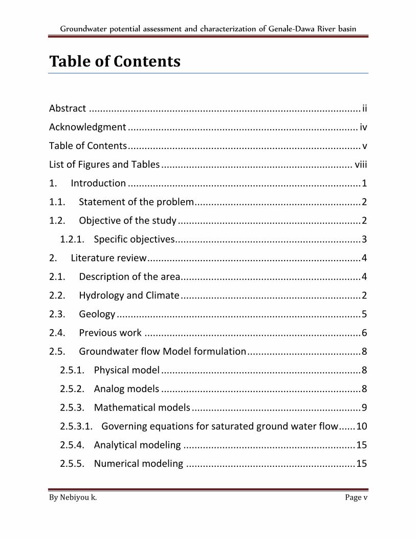
Table of Contents
Abstract .................................................................................................. ii
Acknowledgment ................................................................................... iv
Table of Contents .................................................................................... v
List of Figures and Tables ..................................................................... viii
1. Introduction .................................................................................... 1
1.1. Statement of the problem ............................................................ 2
1.2. Objective of the study .................................................................. 2
1.2.1. Specific objectives ................................................................... 3
2. Literature review ............................................................................. 4
2.1. Description of the area................................................................. 4
2.2. Hydrology and Climate ................................................................. 2
2.3. Geology ........................................................................................ 5
2.4. Previous work .............................................................................. 6
2.5. Groundwater flow Model formulation ......................................... 8
2.5.1. Physical model ........................................................................ 8
2.5.2. Analog models ........................................................................ 8
2.5.3. Mathematical models ............................................................. 9
2.5.3.1. Governing equations for saturated ground water flow ...... 10
2.5.4. Analytical modeling .............................................................. 15
2.5.5. Numerical modeling ............................................................. 15
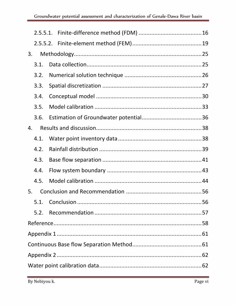
Groundwater potential assessment and characterization of Genale-Dawa River basin
By Nebiyou k. Page vi
2.5.5.1. Finite-difference method (FDM) ........................................ 16
2.5.5.2. Finite-element method (FEM) ............................................ 19
3. Methodology ................................................................................. 25
3.1. Data collection ......................................................................... 25
3.2. Numerical solution technique ................................................. 26
3.3. Spatial discretization ............................................................... 27
3.4. Conceptual model ................................................................... 30
3.5. Model calibration .................................................................... 33
3.6. Estimation of Groundwater potential ...................................... 36
4. Results and discussion................................................................... 38
4.1. Water point inventory data ..................................................... 38
4.2. Rainfall distribution ................................................................. 39
4.3. Base flow separation ............................................................... 41
4.4. Flow system boundary ............................................................ 43
4.5. Model calibration .................................................................... 44
5. Conclusion and Recommendation ................................................ 56
5.1. Conclusion ............................................................................... 56
5.2. Recommendation .................................................................... 57
Reference .............................................................................................. 58
Appendix 1 ............................................................................................ 61
Continuous Base flow Separation Method ............................................ 61
Appendix 2 ............................................................................................ 62
Water point calibration data ................................................................. 62
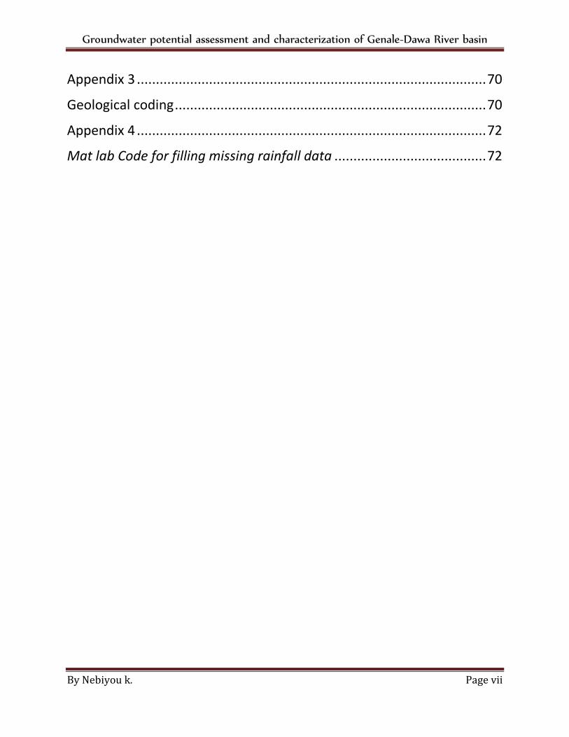
Groundwater potential assessment and characterization of Genale-Dawa River basin
By Nebiyou k. Page vii
Appendix 3 ............................................................................................ 70
Geological coding .................................................................................. 70
Appendix 4 ............................................................................................ 72
Mat lab Code for filling missing rainfall data ........................................ 72
Groundwater potential assessment and characterization of Genale-Dawa River basin
By Nebiyou k. Page viii
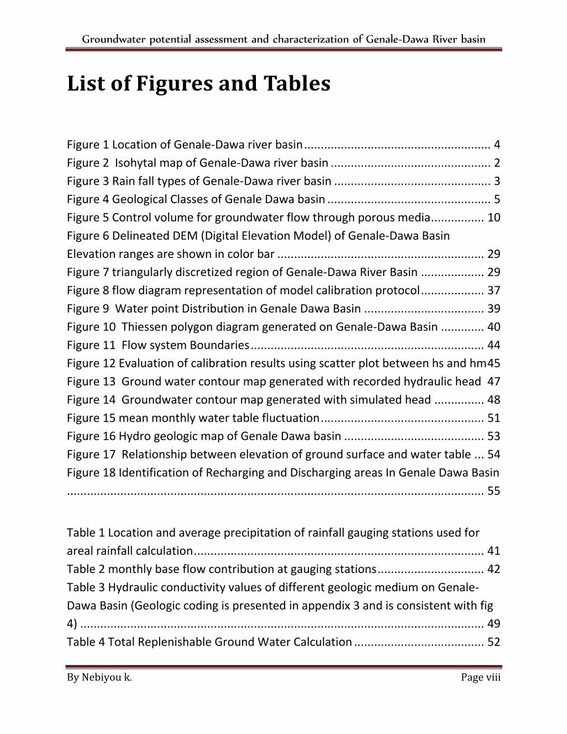
List of Figures and Tables
Figure 1 Location of Genale-Dawa river basin ........................................................ 4
Figure 2 Isohytal map of Genale-Dawa river basin ................................................ 2
Figure 3 Rain fall types of Genale-Dawa river basin ............................................... 3
Figure 4 Geological Classes of Genale Dawa basin ................................................. 5
Figure 5 Control volume for groundwater flow through porous media ................ 10
Figure 6 Delineated DEM (Digital Elevation Model) of Genale-Dawa Basin
Elevation ranges are shown in color bar .............................................................. 29
Figure 7 triangularly discretized region of Genale-Dawa River Basin ................... 29
Figure 8 flow diagram representation of model calibration protocol ................... 37
Figure 9 Water point Distribution in Genale Dawa Basin .................................... 39
Figure 10 Thiessen polygon diagram generated on Genale-Dawa Basin ............. 40
Figure 11 Flow system Boundaries ...................................................................... 44
Figure 12 Evaluation of calibration results using scatter plot between hs and hm 45
Figure 13 Ground water contour map generated with recorded hydraulic head 47
Figure 14 Groundwater contour map generated with simulated head ............... 48
Figure 15 mean monthly water table fluctuation ................................................. 51
Figure 16 Hydro geologic map of Genale Dawa basin .......................................... 53
Figure 17 Relationship between elevation of ground surface and water table ... 54
Figure 18 Identification of Recharging and Discharging areas In Genale Dawa Basin
............................................................................................................................. 55
Table 1 Location and average precipitation of rainfall gauging stations used for
areal rainfall calculation ....................................................................................... 41
Table 2 monthly base flow contribution at gauging stations ................................ 42
Table 3 Hydraulic conductivity values of different geologic medium on Genale-
Dawa Basin (Geologic coding is presented in appendix 3 and is consistent with fig
4) ......................................................................................................................... 49
Table 4 Total Replenishable Ground Water Calculation ....................................... 52
Groundwater potential assessment and characterization of Genale-Dawa River basin
By Nebiyou k. Page 1
1. Introduction
Groundwater is an important natural resource Worldwide. More than 2 billion people depend
on groundwater for their daily supply (Kemper, 2004). It has been estimated that between one
third and one half a billion people in Sub-Saharan African countries use both protected and
unprotected groundwater for their daily water supply. Provided that the initial cost of well
development is in a reasonable order, ground water based water work projects are always
preferable. This is because; Ground water is abundant relative to surface water, dependable in
the sense of amount and usually smaller cost for treatment plant is needed in case where water
is used for domestic supply.
Ethiopia, being one of the most hydrologically blessed countries in east Africa, is believed to
have a large ground water potential. Studies show erroneous results of 2.5 BCM by WAPCOS, to
185 BCM by Ayenew and Alemayehu, in 2001 (Moges, 2012). Which can be taken as an
indication of how much detailed study and survey is needed to estimate the countries
resources with a better precision. This ambiguity in estimation can have a hindering effect on
the countries pursuit to utilize its water resources potential to the limit.
The country’s water supply coverage was estimated to be 30.9 percent, the rural water supply coverage being 23.1 percent and that of urban being 74.4 percent (Semu, 2012). Unpublished reports indicate that susceptibility to drought is higher in the periphery basins of the country such as Genale-Dawa than the central highlands due to high temporal variations of hydrological trends, making it hard to attain sustainable water supply in the region. Moreover, Master Plan Studies carried out during 1997-2007, indicates that Ethiopia has an estimated total potential irrigable land of 3,798,782 ha out of which 1,074,720 ha or 28.3% of the total irrigable land is in the Genale-Dawa River basin (MOWR, Integrated River Basin Master Plan Studies, carrried out during, 2007) Therefore, it can be drawn from the discussion above that, exploring sustainable and drought
proof water resource is of significant importance. As an attempt to contribute to a suitable
solution, this study focuses on evaluating the Genale-Dawa water resource potential and basic
characterization of the ground water system. The study employs 3-D numerical ground water
model to determine the monthly average groundwater table fluctuation, which then is used to
determine the amount of recharge / replenishable ground water potential. The result obtained
is then combined with the result of groundwater potential result by base flow separation
approach.
Groundwater potential assessment and characterization of Genale-Dawa River basin
By Nebiyou k. Page 2
1.1. Statement of the problem
Ethiopia has suffered from repeated drought scenarios in the past; especially the peripheries of
the country like Genale-Dawa basin are more prone to drought than the interior highlands. At
driest seasons even major surface water sources dry up, as a result the available large areas of
suitable irrigation land are left uncultivated and in times, standard domestic water supply
become scarce. As a result proper management and utilization of water resource is vital in the
region. In the past, studies have been done on the region to estimate the water resource
potential. However, even though an estimation of groundwater resource was done based on
different basic approaches in the region, basin wise groundwater numerical modeling has not
been done for the Genale-Dawa catchment. Numerical modeling however is an effective
approach to groundwater potential estimation and also reveals basic characteristics of the flow
system. This can be of significant importance for the detailed understanding of available water
resources and can contribute to the betterment of water resources planning and management.
This study therefore attempts to produce a research output that can be useful for sustainable
use of available groundwater resource.
1.2. Objective of the study
The main objective of this study is to numerically model the ground water flow system of the
study area. There by advance towards detailed understanding of hydro-geological components
of the basin, this can eventually lead to:
Closely approximate the Genale-Dawa river basin ground water potential or
replenishable recharge.
Hydro-geologically characterize the Genale-Dawa Ground water system.
Groundwater potential assessment and characterization of Genale-Dawa River basin
By Nebiyou k. Page 3
1.2.1. Specific objectives
Closely approximate the hydraulic conductivity characteristics and percentage recharge
of the geological classes by performing model calibration.
Determine seasonal groundwater table fluctuation that will be used for estimation of
groundwater potential
Determine base flow contribution of the groundwater flow system to nearby rivers by
doing the necessary data checks, data fill and performing base flow separation.
Hydro-geologically classify the aquifer system based on hydraulic conductivity values
obtained from calibration.
Groundwater potential assessment and characterization of Genale-Dawa River basin
By Nebiyou k. Page 4
2. Literature review
2.1. Description of the area
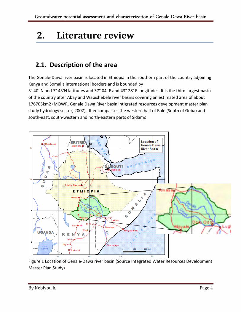
The Genale-Dawa river basin is located in Ethiopia in the southern part of the country adjoining
Kenya and Somalia international borders and is bounded by
3° 40’ N and 7° 43‘N latitudes and 37° 04’ E and 43° 28’ E longitudes. It is the third largest basin
of the country after Abay and Wabishebele river basins covering an estimated area of about
176705km2 (MOWR, Genale Dawa River basin intigrated resources development master plan
study hydrology sector, 2007). It encompasses the western half of Bale (South of Goba) and
south-east, south-western and north-eastern parts of Sidamo
Figure 1 Location of Genale-Dawa river basin (Source Integrated Water Resources Development
Master Plan Study)
Groundwater potential assessment and characterization of Genale-Dawa River basin
Nebiyou k Page 1
The catchment constitutes three river systems namely Dawa, Genale and Wabi Gastro. The
Genale River is joined by Dawa River to form the Genale – Dawa River at the lower portion of
the basin before crossing Ethio-Somali border which drains the western segment of the basin
that is aligned with Omo-gibe river basin. Whereas north-eastern part of the basin is drained by
the Weyeb -Gastro River that meets the Genale – Dawa River near the Ethio-Somalia border to
form the Jubbah River that flows to the Indian ocean (Ethiopian National Meteorological
Agency, 2013).
The southern part of the Southeastern Escarpment of the Main Ethiopia Rift Valley,
Bale and Borena Highlands mark the main head waters of the Genale-Dawa River basin, that
forms the water divide between the Mediterranean and Indian Ocean (Alemayehu, 2006).
Altitude decreases from north to south and from west to east, this variation in altitude ranges
in elevation from more than 4270m.a.m.s.l on the Bale Highlands to less than 173m.a.m.s.l near
the international borders with Somalia and Kenya (south-eastern part of the catchment). Some
20% of the total area lies in the highlands above 1500m and 16% in the lowland plains below
500m (Master plan). The respective sub-basins of the Genale, Dawa and Weyeb Rivers occupy
approximately 33%, 28% and 14% of the total Basin area. The remaining 25% is covered by the
south and eastern border regions, drained by a number of intermittent streams which do not
enter the main river systems (MOWR, Genale Dawa River basin intigrated resources
development master plan study hydro-Geology sector, 2007).
It is mentioned in the integrated master plan that the Genale-Dawa basin area, as pre-
defined by the MOWR and as shown in the previous figure, does not conform to strict
hydrological divisions in the south-west and south-east. This is most apparent on the
extreme south-eastern border in which a sizeable area is assigned to the Wabi-Shebele
basin which actually drains into the Juba River in Genale Dawa basin. A corrected delineation of
the basin is presented on fig. 6 of this study.
Groundwater potential assessment and characterization of Genale-Dawa River basin
Nebiyou k Page 2
2.2. Hydrology and Climate
The basin falls mainly in the arid and semi-arid zone and is generally drought-prone with erratic
rainfall of an average monthly rainfall spacial variation ranging from 34mm to 143mm
(Ethiopian National Meteorological Agency, 2013).
Figure 2 Isohytal map of Genale-Dawa river basin (Source Integrated Resources Development
Master Plan Study)
The temporal variation of Hydrologic characteristics can mainly be described in relation with
migration of the Inter tropical convergence Zone (ITCZ) as briefly described by Camacho, 1977.
A brief review of his work by MOWR master plan describes that
seasonal migration of (ITCZ), which is conditioned by the convergence of trade
winds of the northern and southern hemisphere and the associated atmospheric
circulation. It is also highly influenced, regionally and locally, by the complex topography of the
basin, these accounts for the seasonal climatic changes.
Groundwater potential assessment and characterization of Genale-Dawa River basin
Nebiyou k Page 3
Classifications of rainfall regions based on the seasonal variation of monthly cumulative rainfall
(rainfall type) is also described as follows
Mono-modal: The area designated as region B on Figure 3. is dominated by a single
Peak rainfall pattern in which the relative length of the wet period decrease in a north
direction. Three sub-divisions B1, B2 and B3 have been defined according to duration of wet
period from February/March to October/November and from June/July to
August/September respectively.
Bi-modal Type I: The area designated as region A on Figure 3. is characterised by a quasi-
double peak rainfall pattern with a small peak in April and maximum peak in August.
This region is therefore characterised by a semi-bi-modal rainfall pattern.
Figure 3 Rain fall types of Genale-Dawa river basin (Source Integrated Resources Development Master Plan Study)
Groundwater potential assessment and characterization of Genale-Dawa River basin
Nebiyou k Page 4
Bi-modal Type II: The area identified as region C on Figure 3. is dominated by a double
peak rainfall pattern with similar peaks during April and October. Generally, the annual
rainfall decreases from west to east in the region.
Diffused pattern: The area designated as region D (Danakil region) is characterised by
an irregular rainfall pattern. Though erratic rainfall occurs through the period from
August/September to January/February, the pattern is diffused and not well-defined (MOWR,
Genale Dawa River basin intigrated resources development master plan study, hydrology
sector,, 2007).
Groundwater potential assessment and characterization of Genale-Dawa River basin
Nebiyou k Page 5
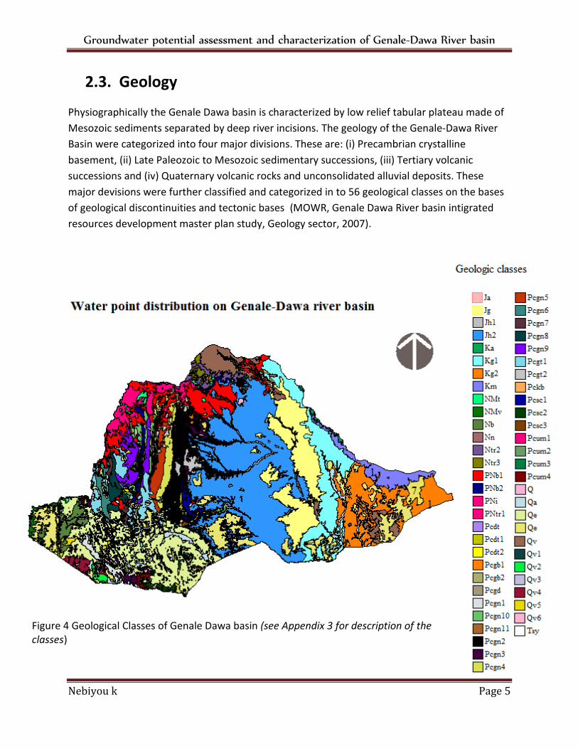
2.3. Geology
Physiographically the Genale Dawa basin is characterized by low relief tabular plateau made of
Mesozoic sediments separated by deep river incisions. The geology of the Genale-Dawa River
Basin were categorized into four major divisions. These are: (i) Precambrian crystalline
basement, (ii) Late Paleozoic to Mesozoic sedimentary successions, (iii) Tertiary volcanic
successions and (iv) Quaternary volcanic rocks and unconsolidated alluvial deposits. These
major devisions were further classified and categorized in to 56 geological classes on the bases
of geological discontinuities and tectonic bases (MOWR, Genale Dawa River basin intigrated
resources development master plan study, Geology sector, 2007).
Figure 4 Geological Classes of Genale Dawa basin (see Appendix 3 for description of the classes)
Groundwater potential assessment and characterization of Genale-Dawa River basin
Nebiyou k Page 6
2.4. Previous work
Several studies were conducted on parts of the basin to generate the geological and Hydro
geological maps on parts of Genale-Dawa basin with different resolution. In parts where
detailed study was needed to identify a well field, electrical resistivity method and GIS and
remote sensing based techniques were devised.
- Alebachew Beyene, Yetnayet Nigussie and Zenaw Tesema in 1987 Prepared Hydro-
geology map of Upper Dawa Basin mainly based on Land seat interpretation with a scale
of 1:500,000. (Beyene, Nigussie, & Tesema, 1987)
- Subsequent to the regional hydrogeological mapping, regional and detailed geo-physical
surveys were conducted `in the Moyale area by (Hailemariam, 1990). This
Survey was also done in the EIGS.
- Regional hydrological and geological works were done in the part at 1:5000000 by ICT
Netherlands students as part of an exercise for their advanced diploma. The ICT
students conducted their Hydro-geological studies by means of aerial photograph and
satellite image interpretation as well as field visits. They have indicated the potential
aquifer sites for ground water development options. (MOWR, Genale Dawa River basin
intigrated resources development master plan study, 2007)
- Ground water potential mapping of Yabelo, a sub catchment of the Genale-Dawa river
basin was carried out to a scale of 1:135000 based on GIS and remote sensing by (Mab
consult – consulting hydro-geologists, 2007)
- Genale-Dawa River Basin Integrated Resources Development Master Plan Study (2000)
was done by MOWE which is detailed basin wise study that briefly covers the geologic
and hydro geologic aspects of the basin at large. This work resulted in generating the
hydro-geological mapping of the basing along with classification of aquifer productivity
based on hydro-geologic features like transitivity and extent of geologic media,
Groundwater potential assessment and characterization of Genale-Dawa River basin
Nebiyou k Page 7
therefore potential water resources development sites were identified ( (MOWR,
Genale-Dawa River Basin Integrated Resources Development Master Plan Study, 2007)).
- The national water resources master plan employed 3 methods for ground water
potential assessment of Genale-Dawa basin namely, Sub surface drainage Approach,
Recharge area approach and Base flow approach was used and ground water potential
of 1.78 BM3 , 0.43BM3 , 0.5 BM3 were obtained respectively (WAPCOS, 2007).
- Hydro-geophysical surveys were conducted by Aklilu et.al and Hailu et.al around Negele
and Filtu towns in 2001. A geophysical method which is VES (Vertical Electrical
Sounding) using schlumberger array was employed to acquire the necessary subsurface
electrical information with 330m minimum AB/2 separation. Consequently areas which
have favorable conditions for groundwater presence were identified around the two
towns (Aklilu & Hilu, 2001).
- Geological and hydro-geological maps of Asela sheet which covers part of the Genale-
Dawa river basin was prepared by (kiflu, tafa, & mulugeta, 2001) to the scale of
1:250,000 with an accompanying report based on both the geological and
hydrogeological information gained during the whole ground water resource
assessment. On the basis of this aquifer systems of the area have been defined and
characterized.
- Other geological sheets have also been investigated in the Genale-Dawa basin
previously. However, Basin wise Numerical models on the Genale-Dawa basin were not
encountered for literature review. Most of the previous works conducted on the
catchment focus mainly on geological and hydro geological mapping of the area in
different scales and resolutions. These can be regarded as a direct approach towards
ground water potential assessment. However, this previous studies have contributed in
raw data and were basic input for conceptualization of current basin wise model
development.
Groundwater potential assessment and characterization of Genale-Dawa River basin
Nebiyou k Page 8
2.5. Groundwater flow Model formulation
A model is a tool designed to represent a simplified version of reality which can be represented
either physically or abstract to capture the significant features of a system. Several types of
groundwater models have been used to study ground water flow systems. They can be divided
into three Broad categories (prickett, 1975): physical models, analog models, including viscous
fluid models and electrical models, and mathematical models, including analytical and
numerical models.
2.5.1. Physical model
Sand tank is the most common type of physical model. In sand tank model, the actual field
dimension was scaled down (three-dimensional) to the laboratory scale and the appropriate
aquifer materials are introduced in the box and the model is simulated by incorporating
appropriate pumping of water from the model and injection of water in to the model and with
appropriate boundary conditions (Thangarajan, Groundwater, Resource Evaluation,
Augmentation, Contamination,Restoration, Modeling and Management, 2007). The major
drawback of sand tank models is the problem of scaling down a field situation to the dimension
of laboratory model. (Herbert F Wang, 1982).
2.5.2. Analog models
An analog model utilizes the similarity of the two physical systems and the one, which is easier
to handle, is used as a model of the other. For example mathematical governing equations of
the physical processes such as flow of electrical current through resistive media or flow of heat
through a solid body are analog physical processes that can be used to model ground water
flow. Viscous Fluid Models, Electric Analog Models, Resistance-Capacitance Analog Modeling
are some of the common Analog models used for ground water modeling. (Thangarajan,
Groundwater, Resource Evaluation, Augmentation, Contamination, Restoration, Modeling and
Management, 2007))
Groundwater potential assessment and characterization of Genale-Dawa River basin
Nebiyou k Page 9
2.5.3. Mathematical models
Mathematical models are abstractions that represent processes as system of equations,
physical properties as constants or coefficients in the equations, and measures of state or
potential in the system as variables. (Delleur, 1999).
Depending up on the nature of equations involved mathematical models can further be divided
in to:
Empirical (experimental): empirical models are derived from experimental data that are fitted
to some mathematical function. (a good example is Darcy’s law)
Probabilistic: probabilistic models are based on laws of probability and statistics. They can have
various forms and complexity starting with a simple probability distribution of a hydro
geological property of inters, and ending with complicated stochastic, distribution of a hydro
geological property of interest and ending with complicated stochastic, time-dependent
models. The main limitations for a wider use of probabilistic models in hydrogeology are: (1)
they require large data sets needed for parameter identification and (2) they cannot be used to
answer the most common questions from hydro geological point of view
Deterministic: Deterministic models assume that the stage or future reactions of the system
studied are predetermined by set of physical laws governing the flow (Anderson & Woessner,
1992).
In the deterministic approach one can see the derivation of groundwater flow governing
equation.
Groundwater potential assessment and characterization of Genale-Dawa River basin
Nebiyou k Page 10
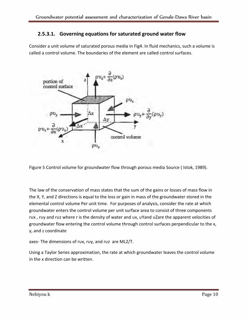
2.5.3.1. Governing equations for saturated ground water flow
Consider a unit volume of saturated porous media in Fig4. In fluid mechanics, such a volume is
called a control volume. The boundaries of the element are called control surfaces.
Figure 5 Control volume for groundwater flow through porous media Source ( Istok, 1989).
The law of the conservation of mass states that the sum of the gains or losses of mass flow in
the X, Y, and Z directions is equal to the loss or gain in mass of the groundwater stored in the
elemental control volume Per unit time. For purposes of analysis, consider the rate at which
groundwater enters the control volume per unit surface area to consist of three components
rυx , rυy and rυz where r is the density of water and υx, υYand υZare the apparent velocities of
groundwater flow entering the control volume through control surfaces perpendicular to the x,
y, and z coordinate
axes- The dimensions of rυx, rυy, and rυz are ML2/T.
Using a Taylor Series approximation, the rate at which groundwater leaves the control volume
in the x direction can be written.
Groundwater potential assessment and characterization of Genale-Dawa River basin
Nebiyou k Page 11
υ υ
υ
υ
+……
If we make the size of the control volume small, we can neglect higher-order terms (i.e, those
involving , , etc) and because we have chosen a unit volume = =1 the net
rate of inflow at the x direction is υ υ
. The net rate of inflow in the x direction is then
Net rate of inflow = rate of inflow in x direction - rate of outflow in x direction
= υ – [ υ υ
]
= υ
And the net rate of inflow in the y and z directions are υ
and
υ
respectively.
According to law of conservation the net rate of inflow or outflow for the entire control volume
must equal to the net change in mass of the control volume.
υ
υ
υ
……… (1)
If we assume that groundwater density, p is constant specially and temporally (i.e., the fluid is
incompressible), we can use the product rule of calculus to evaluate a typical term in the above
equation
υ
υ
υ
But υ
Groundwater potential assessment and characterization of Genale-Dawa River basin
Nebiyou k Page 12
Therefore
υ
υ
Doing similar simplifications for the time component, y direction and z direction and canceling
density that appears outside the derivative (eq. 1) we have
υ
υ
υ
Now the apparent groundwater velocities are given by Darcy's Law
υ
υ
υ
Where , and are the hydraulic conductivities in the x, y, and z directions, respectively
and h is the hydraulic head. Substituting equation AI.7 into equation AI.6. and including
recharge We arrive at the steady-state, saturated/low equation.
If an aquifer parameter is assumed to be homogeneous (at list with in a finite element in case
of numerical modeling), then the chain rule can be employed to get a further simplified
equation
Groundwater potential assessment and characterization of Genale-Dawa River basin
Nebiyou k Page 13
(Jonathan I stole, 1989)
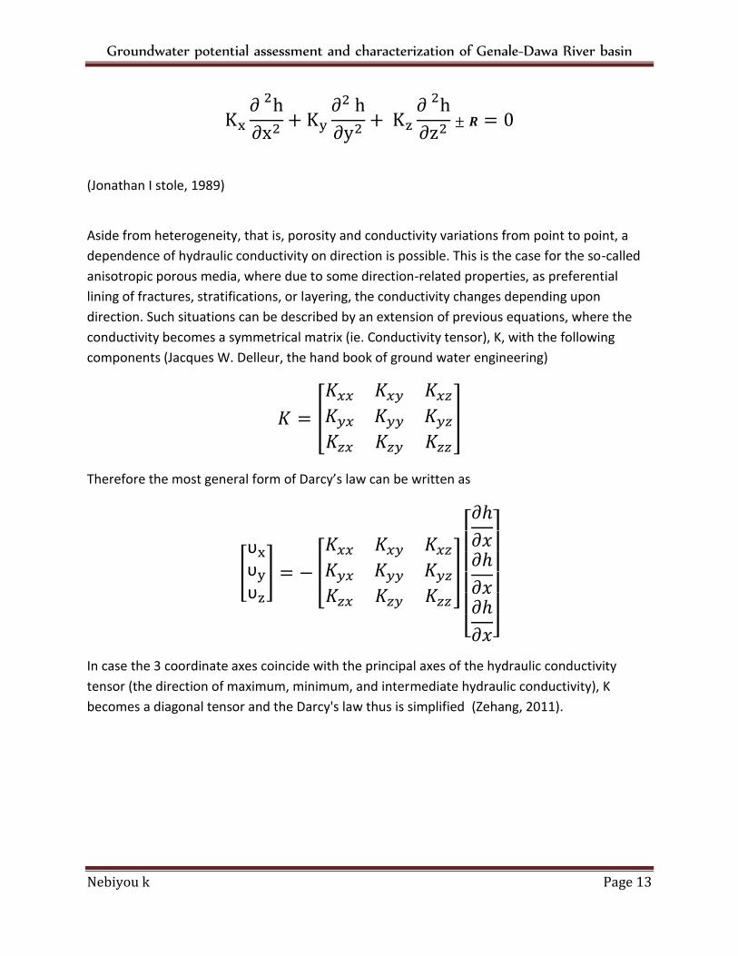
Aside from heterogeneity, that is, porosity and conductivity variations from point to point, a
dependence of hydraulic conductivity on direction is possible. This is the case for the so-called
anisotropic porous media, where due to some direction-related properties, as preferential
lining of fractures, stratifications, or layering, the conductivity changes depending upon
direction. Such situations can be described by an extension of previous equations, where the
conductivity becomes a symmetrical matrix (ie. Conductivity tensor), K, with the following
components (Jacques W. Delleur, the hand book of ground water engineering)
Therefore the most general form of Darcy’s law can be written as
υ
υ
υ
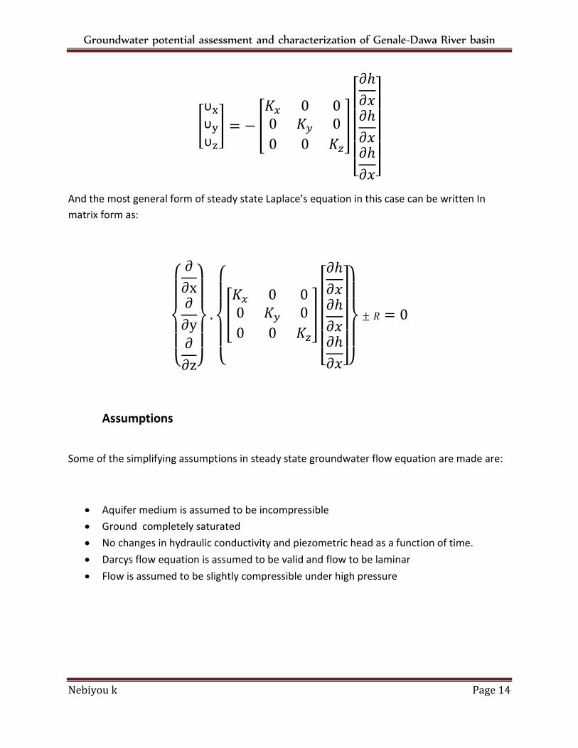
In case the 3 coordinate axes coincide with the principal axes of the hydraulic conductivity
tensor (the direction of maximum, minimum, and intermediate hydraulic conductivity), K
becomes a diagonal tensor and the Darcy's law thus is simplified (Zehang, 2011).
Groundwater potential assessment and characterization of Genale-Dawa River basin
Nebiyou k Page 14
υ
υ
υ
And the most general form of steady state Laplace’s equation in this case can be written In
matrix form as:
Assumptions
Some of the simplifying assumptions in steady state groundwater flow equation are made are:
Aquifer medium is assumed to be incompressible
Ground completely saturated
No changes in hydraulic conductivity and piezometric head as a function of time.
Darcys flow equation is assumed to be valid and flow to be laminar
Flow is assumed to be slightly compressible under high pressure
Groundwater potential assessment and characterization of Genale-Dawa River basin
Nebiyou k Page 15
Limitations
The major limitations of this study include:
The model is tailored to isothermal fully saturated fractured porous medium systems
(solves the Richard’s equation).
In performing a saturated flow analysis, the study handles only single-phase flow of the
liquid (i.e., water) and ignores the flow effects from other potential phases (i.e., air or
other non-aqueous phases) which, in some instances, can be significant.
Deterministic mathematical models of ground water flow problems usually involve partial
differential equations which need to be solved by either analytical or numerical methods.
2.5.4. Analytical modeling
An analytical model aims at obtaining an exact solution of a mathematical description of a
physical process. However, groundwater flow equation, which could be amenable to analytical
techniques, requires several simplifying assumptions of the system including the boundary and
initial conditions. It also requires large computational resource. This process usually renders the
system under study far from being realistic ( (Thangarajan, Groundwater, Resource Evaluation,
Augmentation, Contamination, Restoration, Modeling and Management, 2007)). This method is
usually difficult to employ for large scale groundwater modeling owing to its need for
substantial computational resource
2.5.5. Numerical modeling
Numerical modeling employs approximate methods to solve the partial differential equation
(PDE), which describes the flow in porous medium. The emphasis here is not on obtaining an
exact solution but on obtaining reasonably approximate solution. (Thangarajan, Groundwater,
Resource Evaluation, Augmentation, Contamination,Restoration, Modeling and Management,
Groundwater potential assessment and characterization of Genale-Dawa River basin
Nebiyou k Page 16
2007). Numerical modeling is not subject to many of the restrictive assumptions required for
familiar analytical solutions. Numerical solution normally involves approximating continuous
(defined at every point) partial differential equations with a set of discrete equations in time
(transient model) and space (steady state model). Thus, the region and time period of interest
are divided in some fashion, resulting in an equation or set of equations for each sub region and
time step. These discrete equations are combined to form a system of algebraic equations that
must be solved for specified points in the solution region. Finite-difference and finite-element
methods are the major numerical techniques used in ground water applications the two
methods are presented as follows (Faust & Mercer, 2006).
2.5.5.1. Finite-difference method (FDM)
The finite difference method consists of discretising the problem area into rectangular
elements which are identified with discrete points or nodes ( (Essink, 2000)). Various hydro-
geological parameters are assigned to each of these nodes. Accordingly, difference operators
defining the spatial-temporal relationships between various parameters replace the partial
derivatives. A set of finite difference equations, one for each node is, thus, obtained. In order to
solve a finite difference equation, one has to start with the initial distribution of heads and
compute heads at later time instants ( (Thangarajan, Groundwater, Resource Evaluation,
Augmentation, Contamination,Restoration, Modeling and Management, 2007)).
Groundwater potential assessment and characterization of Genale-Dawa River basin
Nebiyou k Page 17
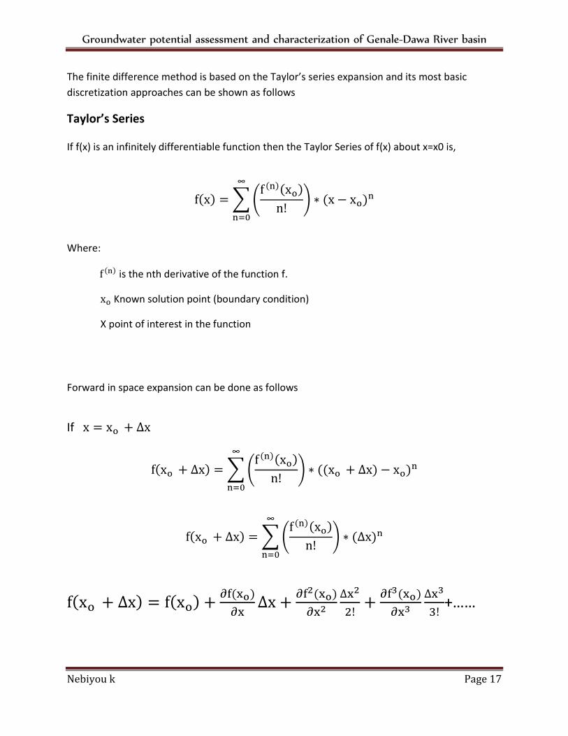
The finite difference method is based on the Taylor’s series expansion and its most basic
discretization approaches can be shown as follows
Taylor’s Series If f(x) is an infinitely differentiable function then the Taylor Series of f(x) about x=x0 is,
Where:
is the nth derivative of the function f.
Known solution point (boundary condition)
X point of interest in the function
Forward in space expansion can be done as follows
If
+……
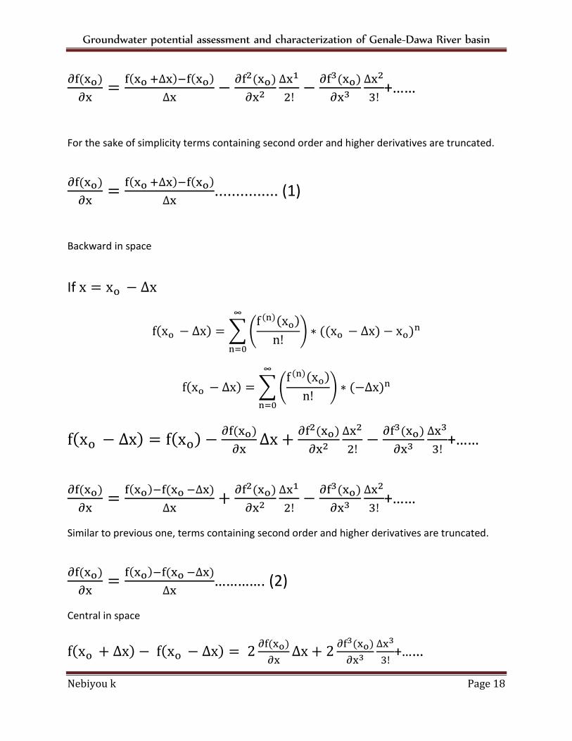
Groundwater potential assessment and characterization of Genale-Dawa River basin
Nebiyou k Page 18
+……
For the sake of simplicity terms containing second order and higher derivatives are truncated.
............... (1)
Backward in space
If
+……
+……
Similar to previous one, terms containing second order and higher derivatives are truncated.
…………. (2)
Central in space
+……
Groundwater potential assessment and characterization of Genale-Dawa River basin
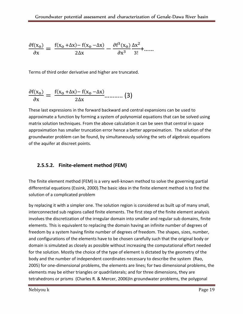
Nebiyou k Page 19
+……
Terms of third order derivative and higher are truncated.
……….. (3)
These last expressions in the forward backward and central expansions can be used to
approximate a function by forming a system of polynomial equations that can be solved using
matrix solution techniques. From the above calculation it can be seen that central in space
approximation has smaller truncation error hence a better approximation. The solution of the
groundwater problem can be found, by simultaneously solving the sets of algebraic equations
of the aquifer at discreet points.
2.5.5.2. Finite-element method (FEM)
The finite element method (FEM) is a very well-known method to solve the governing partial
differential equations (Essink, 2000).The basic idea in the finite element method is to find the
solution of a complicated problem
by replacing it with a simpler one. The solution region is considered as built up of many small,
interconnected sub regions called finite elements. The first step of the finite element analysis
involves the discretization of the irregular domain into smaller and regular sub domains, finite
elements. This is equivalent to replacing the domain having an infinite number of degrees of
freedom by a system having finite number of degrees of freedom. The shapes, sizes, number,
and configurations of the elements have to be chosen carefully such that the original body or
domain is simulated as closely as possible without increasing the computational effort needed
for the solution. Mostly the choice of the type of element is dictated by the geometry of the
body and the number of independent coordinates necessary to describe the system (Rao,
2005) for one-dimensional problems, the elements are lines; for two dimensional problems, the
elements may be either triangles or quadrilaterals; and for three dimensions, they are
tetrahedrons or prisms (Charles R. & Mercer, 2006)In groundwater problems, the polygonal
Groundwater potential assessment and characterization of Genale-Dawa River basin
Nebiyou k Page 20
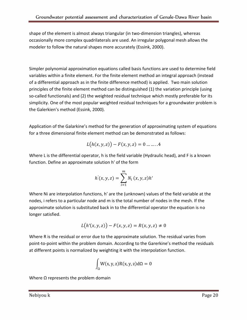
shape of the element is almost always triangular (in two-dimension triangles), whereas
occasionally more complex quadrilaterals are used. An irregular polygonal mesh allows the
modeler to follow the natural shapes more accurately (Essink, 2000).
Simpler polynomial approximation equations called basis functions are used to determine field
variables within a finite element. For the finite element method an integral approach (instead
of a differential approach as in the finite difference method) is applied. Two main solution
principles of the finite element method can be distinguished (1) the variation principle (using
so-called functionals) and (2) the weighted residual technique which mostly preferable for its
simplicity. One of the most popular weighted residual techniques for a groundwater problem is
the Galerkien’s method (Essink, 2000).
Application of the Galarkine’s method for the generation of approximating system of equations
for a three dimensional finite element method can be demonstrated as follows:
Where L is the differential operator, h is the field variable (Hydraulic head), and F is a known
function. Define an approximate solution h of the form
Where Ni are interpolation functions, h are the (unknown) values of the field variable at the
nodes, i refers to a particular node and m is the total number of nodes in the mesh. If the
approximate solution is substituted back in to the differential operator the equation is no
longer satisfied.
Where R is the residual or error due to the approximate solution. The residual varies from
point-to-point within the problem domain. According to the Garerkine’s method the residuals
at different points is normalized by weighting it with the interpolation function.
Where represents the problem domain

Groundwater potential assessment and characterization of Genale-Dawa River basin
Nebiyou k Page 21
To evaluate the above equation, we must specify the mathematical form of the approximate
solution h and the weighting function W. In the finite element method h is defined in a piece -
wise fashion over the problem domain.
‘R’ represents the error between the true value of hydraulic head and the approximate solution
h at that node. The residual at a particular node is the sum of weighted residuals of neighboring
nodes.
The contribution of element e to the residual at node i can be obtained from the integral
formulation for that node. Consider one dimensional case in the x direction with two nodes i
and j
Because the second derivation of a linear interpolation function which is common, is undefined;
expression of the equation in terms of first derivative h
) is needed. The Green’s theorem can
be applied. Negative sign is added for convenience in letter calculation.
The second term in the above equation is given a symbol
for an element and represents
groundwater flow across the element's surface. At the exterior of the mesh this expression
represents rates of boundary condition. Where no flows are specified or at impermeable
aquifer boundaries,
e) will be zero. For elements on the interior of the mesh, the term
for adjacent elements will have opposite signs cancelling out the contribution of
for the
Groundwater potential assessment and characterization of Genale-Dawa River basin
Nebiyou k Page 22
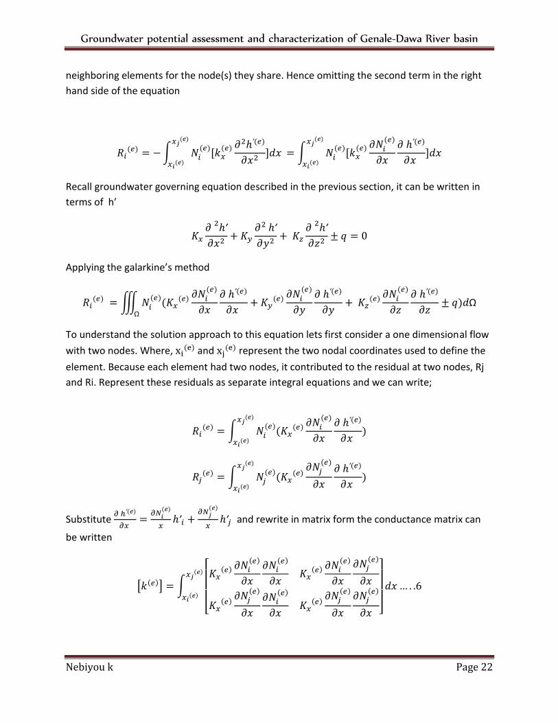
neighboring elements for the node(s) they share. Hence omitting the second term in the right
hand side of the equation
Recall groundwater governing equation described in the previous section, it can be written in
terms of h
Applying the galarkine’s method
To understand the solution approach to this equation lets first consider a one dimensional flow
with two nodes. Where, and
represent the two nodal coordinates used to define the
element. Because each element had two nodes, it contributed to the residual at two nodes, Rj
and Ri. Represent these residuals as separate integral equations and we can write;
Substitute
and rewrite in matrix form the conductance matrix can
be written
Groundwater potential assessment and characterization of Genale-Dawa River basin
Nebiyou k Page 23
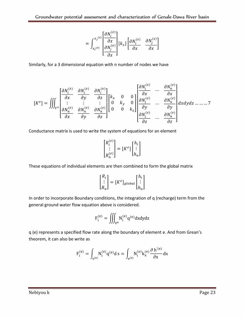
Similarly, for a 3 dimensional equation with n number of nodes we have
Conductance matrix is used to write the system of equations for an element
These equations of individual elements are then combined to form the global matrix
In order to incorporate Boundary conditions, the integration of q (recharge) term from the
general ground water flow equation above is considered.
q (e) represents a specified flow rate along the boundary of element e. And from Grean’s
theorem, it can also be write as
Groundwater potential assessment and characterization of Genale-Dawa River basin
Nebiyou k Page 24
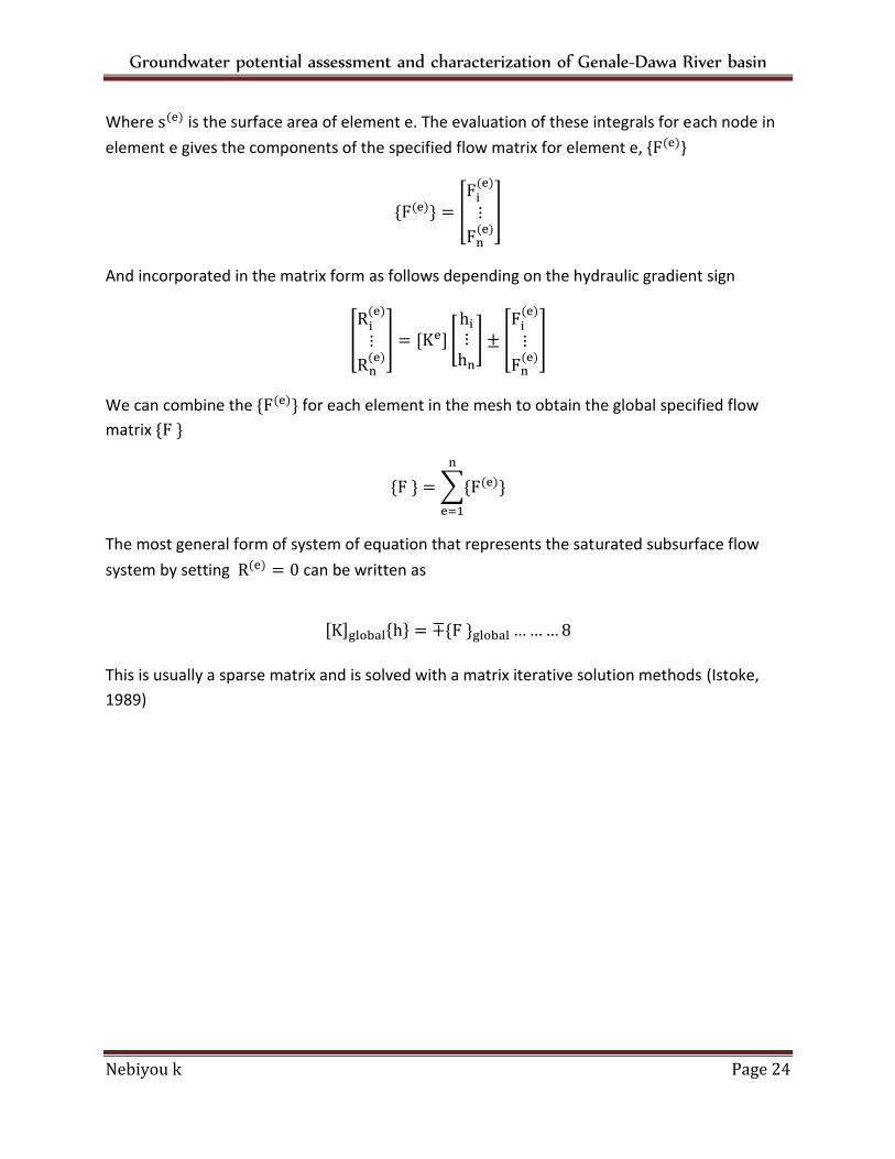
Where is the surface area of element e. The evaluation of these integrals for each node in
element e gives the components of the specified flow matrix for element e, { }
And incorporated in the matrix form as follows depending on the hydraulic gradient sign
We can combine the for each element in the mesh to obtain the global specified flow
matrix
The most general form of system of equation that represents the saturated subsurface flow
system by setting can be written as
This is usually a sparse matrix and is solved with a matrix iterative solution methods (Istoke,
1989)
Groundwater potential assessment and characterization of Genale-Dawa River basin
Nebiyou k Page 25
3. Methodology
Assessment of ground water potential can be achieved through various methodologies. This
chapter focuses on explaining how the FEM modeling approach was adopted for the regional
groundwater potential assessment of the current study area.
3.1. Data collection
Various relevant raw data that can reveal an insight of the subsurface reservoir and softwares
useful for modeling were collected. These are:
Softwares used for the model development, including;
Mat lab v.13a: where numerical calculations are carried out and the TAGSAC code is run.
Global Mapper v.16, Surfer v.10: used for surveying works, delineation, digitization, data
manipulation and data pre processing.
Hydrogeologic data
1:2000, 000 resolution geological map with 56 geological classes were collected.
Springs and well inventory data.
30×30m resolution Digital elevation model of the region in which Genale-Dawa River
basin is located.
Hydrologic data
Rain fall data records of 23 gauging stations near and on the basin.
Stream flow data of some gauging station on the basin; this was used to develop an
understanding of the overall hydro geological system and also, determine aquifer
contribution to the rivers by performing base flow separation.
Groundwater potential assessment and characterization of Genale-Dawa River basin
Nebiyou k Page 26
3.2. Numerical solution technique
Laplace’s equation as described in the previous chapter is a general equation that governs
groundwater flow system and other analogous systems like conductance of heat with in a solid
body. In mathematical modeling of groundwater this equation needs to be solved either
analytically or numerically. Analytical solutions can be used to calculate values for the unknown
field variable at any point in the problem domain. Whereas, numerical solutions yield values for
only a predetermined finite number of points in the problem domain. Considering the
complexity of the problem; the numerical method is chosen for this study. And from the two
well known numerical methods available the (finite element and finite difference) the finite
element is selected considering its computational efficiency. This is due to the following
reasons:
1) FEM is more suited to better discretising a given solution region owing to the use of
unlimited discretising element shape and size.
2) Because different type and degree of approximation equations can be used, it can better
approximate the solution compared to the FDM, which can be considered as a method that
uses linear interpolation between two points towards determining field variable at succeeding
discrete points. (The Finite Element Method, O.C. Zienkiewicz and R.L. Tylor, 2000, by
butterworth-Heinemann, England)
A particular type of FEM based three dimensional computer modeling code called TAGSAC
(Three Dimensional Analysis of Groundwater Flow, Saitama University Code) is adopted for
modeling the groundwater system. TAGSAC is a model developed for the porous medium. In
the TAGSAC approximation procedure, the flow region is first discretized into a network of
finite elements, and then trial approximating interpolation functions are generated for
individual finite elements using a special type of weighted residual method called Galerkin’s
method; in which the summation of residuals weighted by interpolation functions is equated to
zero. This results in a system of linear interpolation functions. By incorporating boundary
conditions and solving, coefficients of interpolation functions are obtained. This system of
equations is used to represent the unknown dependent variable (hydraulic head) over the
discretized region. A limiting feature of TAGSAC model is that it is bound to use a model
thickness not less than half the finite elements dimension used; which otherwise will risk
Groundwater potential assessment and characterization of Genale-Dawa River basin
Nebiyou k Page 27
numerical instability. Tagsac Has Proved To Be Applicable In A Number Of Researches Done All
Over The Globe (Mohammed, 2010).
3.3. Spatial discretization
The first step of the finite element analysis involves discretization of the irregular domain into
smaller and regular sub domains. This is equivalent to replacing the domain having an infinite
number of degrees of freedom by a system having finite number of degrees of freedom. The
following section is dedicated to describe the discretization processes.
The geometric representation of the system shall first be established for which, Cartesian
coordinate system is employed to generate a triangular in plane three dimensional mesh. The x-
y plane coincides with plane view of the study area where as z direction point’s perpendicularly
in the upward direction to the x-y plane, representing elevation.
An initial step taken for discretization was to delineate the Genale-Dawa catchment area which
was done using Global Mapper version 16 and using digital elevation model of 30×30m
resolution. The result obtained was a little different than the official delineated map of Genale-
Dawa basin used by MOWE in that the delineation result obtained and to be used for this study
has some additional area on the south-eastern part of the basin with a total of 17860km2 km2.
This, in recent master plan study of the basin was recognized as covered in the literature review
part of this paper.
After the delineation x-y coordinates of the catchment boundary are generated and used as
problem domain of the model. The discretization elements are made to be non uniform in size
to best fit the boundaries of the problem domain where there are Sharpe corners. A maximum
of 5km edge dimension for the equilateral triangular finite element is selected. This done
considering the available computational capacity and level of details of raw data available. The
problem domain of 17860km2 area is then discretized in to 9810 nodes of known x-y
coordinates with consistent and continuous nodal numbering assigned to them. 17862
triangular elements are formed by connecting three neighboring nodes with a line. This
geometric discretization of the region is first done on x-y plane and is carried out using
automatic discretising Mat lab computer code. The z coordinate of the nodal points of the mesh
is tabulated by interpolation from the digital elevation model. After wards this triangular mesh
so formed is given a model thickness of 2500m to form the three dimensionally discretized
Groundwater potential assessment and characterization of Genale-Dawa River basin
Nebiyou k Page 28
systems. Hence, each triangular two dimensional element was changed in to three dimensional
finite element formed with six nodal points in space and becomes a prism that is triangular in
plain. Boreholes and springs are represented by 3 nearest surface nodes where as River
systems are made to traverse along a series of surface nodes; this is done by moving the
nearest surface node to the river at a point using a mat lab code. Relocation of the top layer
nodes near a river causes vertical distortion of the prismatic finite elements that can be
handled by TAGSAC.
Finally, individual elements and surface nodal points are given codes that designate the
material property and rainfall recharge amount respectively to the individual elements and
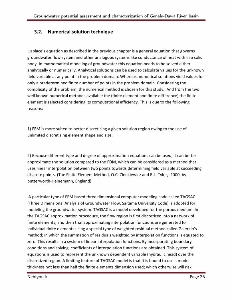
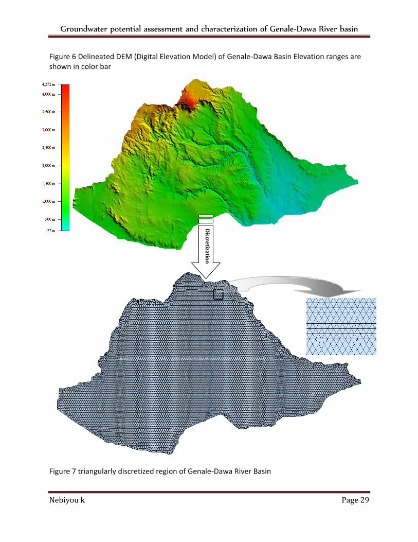
surface nodes. Fig. 6 and Fig 7 Respectively shows the geometrically discretized domain and
geologic materials assigned for each discreet triangular element by coloring the element
centroid with different classes of colors.
Groundwater potential assessment and characterization of Genale-Dawa River basin
Nebiyou k Page 29
Figure 6 Delineated DEM (Digital Elevation Model) of Genale-Dawa Basin Elevation ranges are shown in color bar
Figure 7 triangularly discretized region of Genale-Dawa River Basin
Discre
tization
Groundwater potential assessment and characterization of Genale-Dawa River basin
Nebiyou k Page 30
3.4. Conceptual model
3.4.1. Conceptualization of flow medium
Several conceptual groundwater flow models have be distinguished on the basis of the storage
and flow capabilities of the porous medium and fracture. The storage characteristics are
associated with porosity, and the flow characteristics are associated with permeability. Three
conceptual models have dominated the research: 1) dual continuum, 2) discrete fracture
network, and 3) single equivalent continuum. In addition, Explicit discrete fracture, multiple-
interacting continua and multi-porosity/multi-permeability conceptual models (Sahimi, 1995)
have been introduced in the literature. For the sake of discussion the first 3 are presented
below
Discrete Fracture Network Discrete fracture network (DFN) models describe a class of dual-continuum models in which the
porous medium is not represented. Instead, all flow is restricted to the fractures. This
idealization reduces computational resource requirements. Fracture “legs” are often
represented as lines or planes in two or three dimensions (Sarkar, Toksöz, & Burns). The DF
approach is typically applied to fractured media with low primary permeability such as
crystalline rock. (Anderson & Woessner, 1992).
Dual-continuum models
Dual-continuum models are based on an idealized flow medium consisting of a primary porosity
created by deposition and lithification and a secondary porosity created by fracturing, jointing,
or dissolution. The basis of these models is the observation that un-fractured rock masses
account for much of the porosity (storage) of the medium, but little of the permeability (flow).
Conversely, fractures may have negligible storage, but high permeability (Sarkar, Toksöz, &
Burns).
Groundwater potential assessment and characterization of Genale-Dawa River basin
Nebiyou k Page 31
Single Equivalent Continuum Formulation
Fractured material is represented as an equivalent porous medium by replacing the primary
and secondary porosity and hydraulic conductivity distributions with a continuous porous
medium having so called equivalent hydraulic properties (Anderson & Woessner, 1992). This
method is most suited to the condition in which the volume of interest is considered to be large
enough that, on average, permeability is a sum of fracture and porous media permeability. This
approximation substantially simplifies the flow problem (Diodato, 1994).
This study employs the single equivalent continuum conceptual modeling approach in which
the hydraulic parameters are selected so that the; flow pattern in the discretized elements is
similar to the flow pattern in the actual fractured system. This formulation methodology is
adopted, taking in to account the sizes of the (Representative Elementary Volume) REV
considered being large and the moderate availability of computational resources. (Istoke,
1989)
3.4.2. Ground water recharge
Recharge is defined as the downward flow of water reaching the water table forming an
addition to the ground water reservoir (Vries & Simmer, 2000). It is also defined as a term used
to describe many of the processes involved in the addition of water to the saturated zone
(Moore & Wilson, 1998). When the front of infiltrating water reaches the capillary fringe
(percolates), it displaces air in the pore spaces and causes the water table to rise along with the
capillary fringe (Applied hydrology ground water).
Groundwater recharge rate, as briefly described by (Healy, 2010), is both specially and
temporally varied. This variability is due to a number of factors such as; climate, soil cover,
geology, surface topography, hydrology and vegetation cover. Therefore, a good recharge
estimation for a given study area; requires a clear understanding of the factors in play for the
specific site under study. This usually, is not an easy task to achieve because of both financial
and techniqueal difficulties faced with. However, some methods such as Chemical tracer
methods, Water-budget methods and numerical modeling methods in which Recharge
estimates can be obtained through a model calibration process with recharge rate as a
calibration parameter (Healy, 2010)can be used to get a close estimation.
Major natural recharge to the unconfined aquifer system in the current study area occurs at
elevated regions due to percolation from precipitation along the north, north-eastern and
north-western boundary highs of the basin. Whereas recharge from runoff and precipitation on
the lower part of the basin also provides a source of groundwater inflow to the area of interest.
Groundwater potential assessment and characterization of Genale-Dawa River basin
Nebiyou k Page 32
This study tries to estimate the replenishable groundwater resource (from hydrological
perspective) using the TAGSAC model by seating precipitation to be some portion of the total
rainfall in percent and making this percentage a calibration parameter that can be obtained
through a series of trial and error procedure.
3.4.3. Model Boundary conditions
It is crucial to define a boundary condition prior to numerical groundwater model development.
This is because, the solution of Laplace’s equation requires specification of boundary conditions
which constrain the problem and make solutions unique (Anderson & Wosner, 1992).Hence,
boundary conditions are known solutions at points in the solution domain necessary to obtain
solution at unknown points representative of the real system. P.Anderson and W.Wosner have
distinguished the different types of boundary condition.
Which are described as follows:
A) head is known for surfaces bounding the flow region (Dirichlet Conditions);
B) flow is known across surfaces bounding the region (Newman condition)
C) a combination of Dirichlet and Newman conditions known as mixed condition
The most common types of boundary conditions are; perennial rivers, springs, lakes and swampy areas known to have ground water reserve underneath, all of which can be taken as Dirichlet boundary conditions after a careful observation of their relation with the aquifer nearby and the hydraulic property of intermediate medium. On the other hand; known amount of inter-aquifer leakage, water wells and springs of known discharge can be taken as Newman’s conditions. The determination of which aspects of an actual ground-water system should be incorporated into a computer simulation usually depends, in part, upon the objectives of the study for which the model is being developed (Reilly, 2001) accordingly in constant head constant discharge and specified flow boundary conditions have been identified for the current modeling.
Groundwater potential assessment and characterization of Genale-Dawa River basin
Nebiyou k Page 33
3.4.4. Hydraulic properties
Hydraulic properties important for the three dimensional conceptual model include both
horizontal and vertical hydraulic conductivities as well as specific storage coefficient. In order to
generate the numerical model of the site, the distribution of these parameters must be
specified for each hydro-geological unit. However since the model is based on the principles of
equivalent porous medium, Hydraulic properties are assumed to be equivalent or effective
values for the 56 individual geological class. These geological classes have been discretized and
Equivalent hydraulic properties are obtained by calibration procedure for respective geological
classes.
3.4.5. Water points inventory
Water point inventory data is comprehensive data collected about the water points. Inventory
data of water points on the basin include data about water wells, hand dug wells and springs.
The details of this data include static water level and coordinates of individual water wells and
springs. Which is important for the model calibration process, as it is evident information
available regarding the regional groundwater condition. The water point inventory data
collection on the basin was carried out using dip meters and GPS instruments.
3.5. Model calibration
Model calibration is the process of adjusting the input properties and boundary conditions of a
model to achieve a close fit to observed conditions in the real groundwater system. In flow
model calibration, simulated heads and discharges are typically compared to their observed
counterparts. If a model is well calibrated, there will be some random deviations between
simulated and observed data, but there will not be systematic deviations. If there are
systematic deviations such as most simulated heads exceeding observed heads, the calibration
is poor and adjustments should be made (fitts, 2002).
Groundwater potential assessment and characterization of Genale-Dawa River basin
Nebiyou k Page 34
As discussed by (Kresic, 2009) , there are two methods of calibration:
(1) Trial and error (manual) and
(2) Automated calibration.
In the trial and error approach, the user inputs all the parameters that can be based on physical
observation, and provides estimates of the unknown parameters as a first trial. As such, the
adjustment of parameters is manual. The model is run and the computed output is compared
to the measured output from the model. Most of the time the transmissivities are the least
known parameters and thus, they are often modified during the calibration procedure. The
comparison is done either by means of visual pattern, or it is based on some mathematical
criterion. Based on this comparison, adjustments are made to one or more of the trial
parameters to improve the fit between measured and computed output. In an effort to get the
best fit between measured and computed output, it helps to go back to the basic principle
stated by Darcy
in which the relationship between h ,k and q can be used as a
rule of thumb in calibration. If for example the measured head is larger than the computed. As
it can be seen from Darcy’s law; reducing the hydraulic conductivity in some proportion would
result in larger head to be computed (close to the observed head) by the model and vice versa
(fitts, 2002). Hence, a systematic trial and error (manual) calibration can be achieved. These
trial runs of the model are repeated until some kind of required accuracy or calibration target is
achieved (Essink, 2000). Trial and error calibration was the first technique applied in
groundwater modeling and is still preferred by most users (Kresic, 2009). Whereas on the other
hand automated calibration method employs a computer program that will automatically
calibrate itself and carry out the necessary number of trial runs until the best set of parameters
is achieved. The purpose of this program is to minimize an objective function such as to
minimize the sum of the square residuals. Though this approach is advantageous for that it
gives statistical degree of uncertainty and saves time. It should also be kept in mind that it can
also give unstable and unreasonable results. This paper employs the trial and error calibration
procedure as described earlier. The protocol followed in the modeling and calibration is shown
using a flow diagram described in figure 8.
Groundwater potential assessment and characterization of Genale-Dawa River basin
Nebiyou k Page 35
3.5.1. Calibration Evaluation
The result of the calibration should be evaluated both qualitatively and quantitatively
(Anderson & Wosner, 1992)
(a) Qualitatively, by comparison of contour maps of measured and computed parameters,
which provides only a qualitative measure of the similarity between the patterns; and
(b) Quantitatively, by a scatter plot of measured and computed parameters, where the
deviation of points from the straight line should be randomly distributed (Essink, 2000). In an
effort to minimize the error in the calibration, the average deviation is calculated using the
mean error (ME), mean absolute error (MAE) and root mean squared error (RMS) indicators,
the calibration is continued until these indicators are satisfactorily minimized.
1. The mean error (ME)
2. The mean absolute error (MAE)
3. The root mean squared error (RMS)
Groundwater potential assessment and characterization of Genale-Dawa River basin
Nebiyou k Page 36
The maximum acceptable value of calibration criterion depends on the magnitude of the
change in head over the problem domain (Anderson and Woessner, 1992). The scatter diagram
generated by model also shows the matching property of the measured simulated head. The
scatter plot is usually examined by the position of points scattered in the graph away from the
straight line, that is; random distribution of point in the plot shows the deviation between
measured and simulated groundwater heads.
3.5.2. Model calibration Target
A calibration target consists of the best estimate of a value of groundwater head or flow rate. Establishment of calibration targets and acceptable residuals or residual statistics depends on the degree of accuracy proposed for a particular model application. This, in turn, depends strongly upon the objectives of the modeling project (ASTEM, 2008). For any particular calibration target, the magnitude of the acceptable residual depends partly upon the magnitude of the error associated with data collection. Head measurements in particular are usually accurate to within a few tenths of a foot. Due to the many approximations employed in modeling and errors associated therewith, it is usually impossible to make a model reproduce all head measurements within the errors of measurement. This incompatibility can be adjusted by taking data collection error in to account and providing a range of acceptable errors for the model output. As stated by ASTEM (D5981 – 96), the acceptable residual should be a small fraction of the
difference between the highest and lowest heads across the site.
3.6. Estimation of Groundwater potential
After the model calibration, monthly water table fluctuation is calculated. This helps
determinine the maximum water table, minimum water table and eventually the change in
storage of the groundwater system within a year. This amount of water is known as the
replenishable groundwater which represents the recharge capacity of the system. But, even
though in a given month the aquifer is assumed to have a given amount of groundwater storage
Groundwater potential assessment and characterization of Genale-Dawa River basin
Nebiyou k Page 37
with an associated water table it also discharges to the rivers at the same time. Hence, base
flow separation is done using digital filter method to account for the water at the discharging
end of the system and the cumulative groundwater reserve is calculated for individual months.
Finally based on calibration results hydraulic conductivities of different geologic classes are
grouped to generate the different hydro-geologic classes of the region and prepare
Hydrogeologic map of the region.
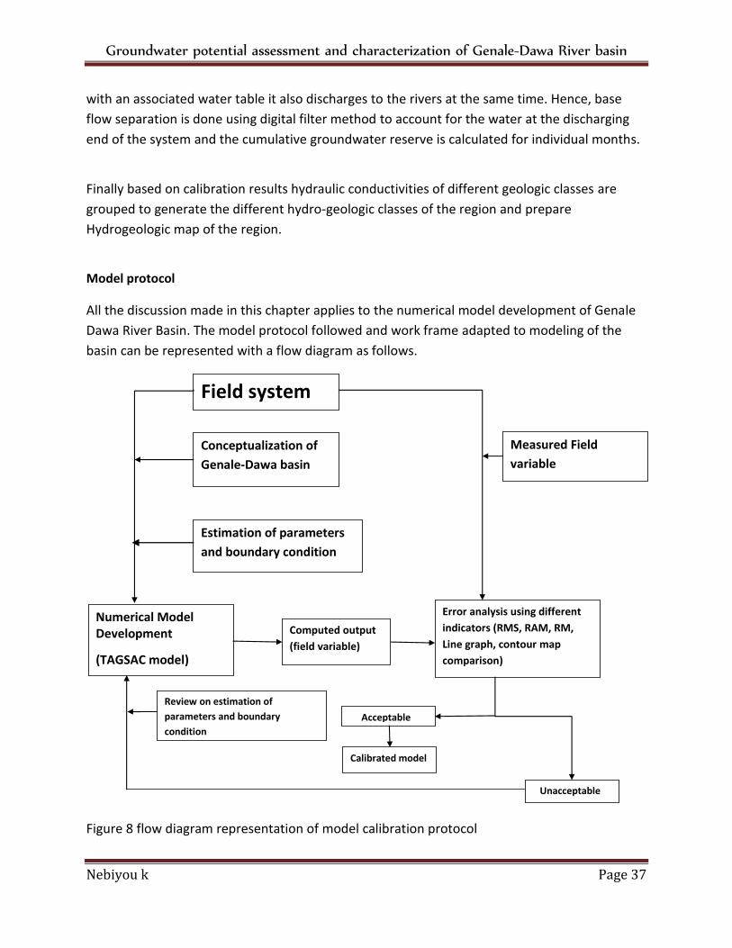
Model protocol
All the discussion made in this chapter applies to the numerical model development of Genale
Dawa River Basin. The model protocol followed and work frame adapted to modeling of the
basin can be represented with a flow diagram as follows.
Figure 8 flow diagram representation of model calibration protocol
Field system
Conceptualization of
Genale-Dawa basin
Estimation of parameters
and boundary condition
Numerical Model Development
(TAGSAC model)
Measured Field
variable
Calibrated model
Error analysis using different
indicators (RMS, RAM, RM,
Line graph, contour map
comparison)
Acceptable
Unacceptable
Computed output
(field variable)
Review on estimation of
parameters and boundary
condition
Groundwater potential assessment and characterization of Genale-Dawa River basin
Nebiyou k Page 38
4. Results and discussion
The methodology described in the previous chapter was employed to develop a three
dimensional numerical single layered groundwater model for the evaluation of replenishable
groundwater potential. Results and relevant discussions of the model are presented in this
chapter in their chronological order.
4.1. Water point inventory data
Water point inventory data relevant for the model calibration was collected from concerned
offices. This included; bore hole, hand dug well and spring data of Genale-Dawa River basin.
Out of these collected data, some data was omitted for not qualifying to contain either the
static water level or coordinate information. A secondary data screening was also done by
comparing recorded static water level with expected result from the model. Accordingly,
personal judgment was taken to discard where large data inconsistency is observed. After
screening 82 Bore holes, 49 hand dug wells and 191 spring data were left to be used as an input
for the model.
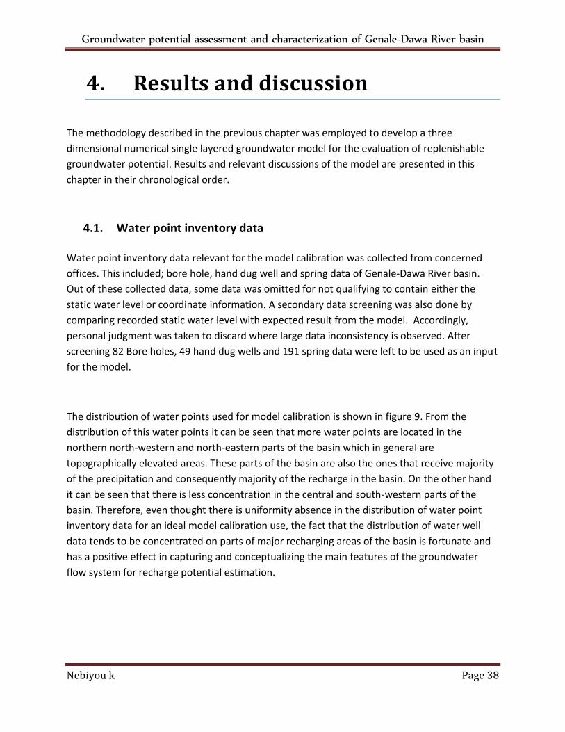
The distribution of water points used for model calibration is shown in figure 9. From the
distribution of this water points it can be seen that more water points are located in the
northern north-western and north-eastern parts of the basin which in general are
topographically elevated areas. These parts of the basin are also the ones that receive majority
of the precipitation and consequently majority of the recharge in the basin. On the other hand
it can be seen that there is less concentration in the central and south-western parts of the
basin. Therefore, even thought there is uniformity absence in the distribution of water point
inventory data for an ideal model calibration use, the fact that the distribution of water well
data tends to be concentrated on parts of major recharging areas of the basin is fortunate and
has a positive effect in capturing and conceptualizing the main features of the groundwater
flow system for recharge potential estimation.
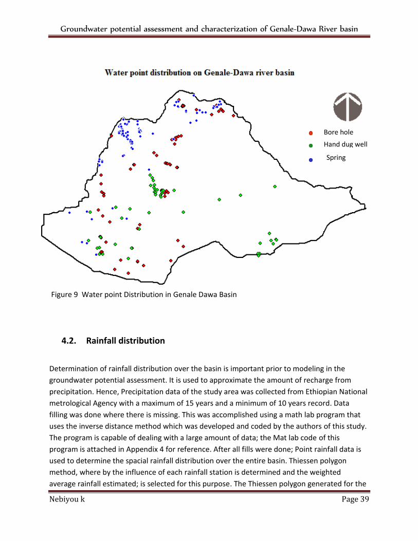
Groundwater potential assessment and characterization of Genale-Dawa River basin
Nebiyou k Page 39
Figure 9 Water point Distribution in Genale Dawa Basin
4.2. Rainfall distribution
Determination of rainfall distribution over the basin is important prior to modeling in the
groundwater potential assessment. It is used to approximate the amount of recharge from
precipitation. Hence, Precipitation data of the study area was collected from Ethiopian National
metrological Agency with a maximum of 15 years and a minimum of 10 years record. Data
filling was done where there is missing. This was accomplished using a math lab program that
uses the inverse distance method which was developed and coded by the authors of this study.
The program is capable of dealing with a large amount of data; the Mat lab code of this
program is attached in Appendix 4 for reference. After all fills were done; Point rainfall data is
used to determine the spacial rainfall distribution over the entire basin. Thiessen polygon
method, where by the influence of each rainfall station is determined and the weighted
average rainfall estimated; is selected for this purpose. The Thiessen polygon generated for the
Bore hole
Hand dug well
Spring
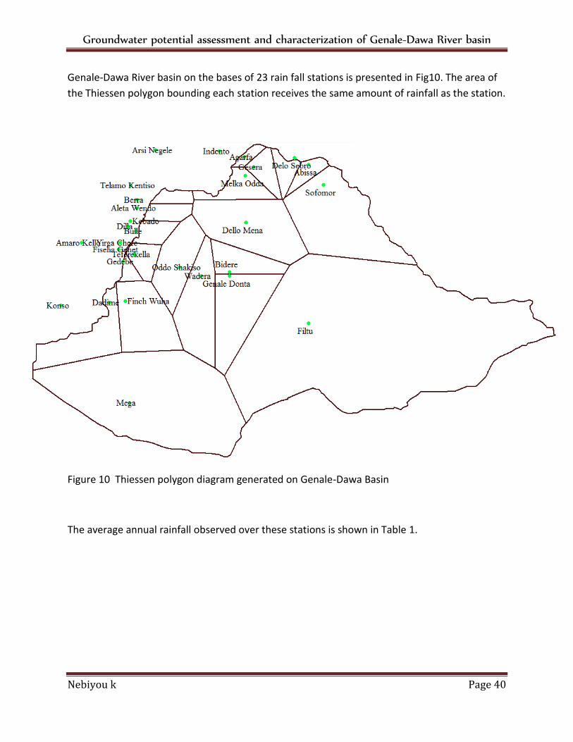
Groundwater potential assessment and characterization of Genale-Dawa River basin
Nebiyou k Page 40
Genale-Dawa River basin on the bases of 23 rain fall stations is presented in Fig10. The area of
the Thiessen polygon bounding each station receives the same amount of rainfall as the station.
Figure 10 Thiessen polygon diagram generated on Genale-Dawa Basin
The average annual rainfall observed over these stations is shown in Table 1.
Groundwater potential assessment and characterization of Genale-Dawa River basin
Nebiyou k Page 41
Table 1 Location and average precipitation of rainfall gauging stations used for areal rainfall
calculation
No. Met. station Location (UTM) Annual cumulative of monthly Mean rainfall
Station Code Latitude, N Longitude, E (mm)
1 ABISSA (S-21) 70952 403855 747.8054708
2 SOFOUMER (S-20) 65400 405024 585.4909383
3 KEBADO(S-2) 62600 382000 1398.618571
4 FISHA GENET(S-6) 60400 381100 1394.102499
5 YIRGA CHEFE(S-5) 60902 381207 1333.485122
6 FILTU(S-12) 50623 403835 408.485119
7 MEGA(S-11) 40413 381914 615.2595465
8 GENALE DONTA(S-13) 54300 393700 1297.203825
9 DADIME (S-10) 52228 380330 758.3530511
10 FINCH WUHA (S-19) 52335 381611 765.9513511
11 GEDEBE(S-7) 55420 381422 1517.122361
12 BIDER (S-14) 54600 393700 781.2535876
13 WADERA (S-15) 54300 391500 898.3692765
14 ODDO SHAKISO (S-16) 55000 385800 1022.980829
15 TEFERKELA (S-8) 60000 382300 1724.167539
16 BULLE (S-1) 61813 382414 1533.079242
17 ALETA WONDO(S-3) 63614 382505 1582.162685
18 BERRA(S- 4) 64236 382505 1303.217431
19 DELLO MENA (S-17) 62500 395000 1021.439937
20 MELKA ODDA (S-18) 70116 394934 559.8847648
21 AGARFA (S-22) 71600 394900 1086.15793
22 GESERA (S-19) 70800 395600 1007.416663
23 DELLO SIRBO (23) 71500 402800 1023.40185
4.3. Base flow separation
Monthly stream flow data of 12 gauging stations over the basin was collected. The length of
data record ranges from 15 to 20 yrs. prior to using these data for the determination of base
flow contribution to rivers, data filling and quality check was done using outlier testing as
shown below. Data filling was done using single and multiple regression techniques
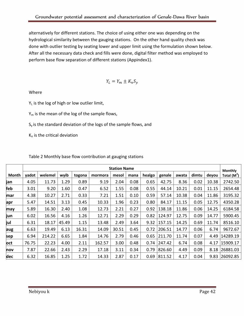
Groundwater potential assessment and characterization of Genale-Dawa River basin
Nebiyou k Page 42
alternatively for different stations. The choice of using either one was depending on the
hydrological similarity between the gauging stations. On the other hand quality check was
done with outlier testing by seating lower and upper limit using the formulation shown below.
After all the necessary data check and fills were done, digital filter method was employed to
perform base flow separation of different stations (Appindex1).
Where
YL is the log of high or low outlier limit,
Ym is the mean of the log of the sample flows,
Sy is the standard deviation of the logs of the sample flows, and
Kn is the critical deviation
Table 2 Monthly base flow contribution at gauging stations
Month
Station Name Monthly Total (M
3) yadot welemel wyib togona mormora mesol mana healgo genale awata dimtu deyou
jan 4.05 11.73 1.29 0.89 9.19 2.04 0.08 0.65 42.75 8.36 0.02 10.38 2742.50
feb 3.01 9.20 1.60 0.47 6.52 1.55 0.08 0.55 44.14 10.21 0.01 11.15 2654.48
mar 4.38 10.27 2.71 0.33 7.21 1.51 0.10 0.59 57.14 10.38 0.04 11.86 3195.32
apr 5.47 14.51 3.13 0.45 10.33 1.96 0.23 0.80 84.17 11.15 0.05 12.75 4350.28
may 5.89 16.30 2.40 1.08 12.73 2.21 0.27 0.92 138.18 11.86 0.06 14.25 6184.58
jun 6.02 16.56 4.16 1.26 12.71 2.29 0.29 0.82 124.97 12.75 0.09 14.77 5900.45
jul 6.31 18.17 45.49 1.15 13.48 2.49 3.64 9.32 157.15 14.25 0.69 11.74 8516.10
aug 6.63 19.49 6.13 16.31 14.09 30.51 0.45 0.72 206.51 14.77 0.06 6.74 9672.67
sep 6.94 214.22 6.65 1.84 14.76 2.79 0.46 0.65 211.70 11.74 0.07 4.49 14289.19
oct 76.75 22.23 4.00 2.11 162.57 3.00 0.48 0.74 247.42 6.74 0.08 4.17 15909.17
nov 7.87 22.66 2.43 2.29 17.18 3.11 0.34 0.79 826.60 4.49 0.09 8.18 26881.03
dec 6.32 16.85 1.25 1.72 14.33 2.87 0.17 0.69 811.52 4.17 0.04 9.83 26092.85
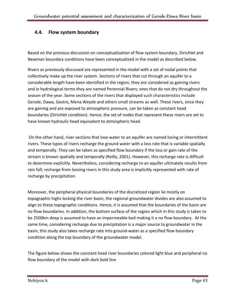
Groundwater potential assessment and characterization of Genale-Dawa River basin
Nebiyou k Page 43
4.4. Flow system boundary
Based on the previous discussion on conceptualization of flow system boundary, Dirichlet and
Newman boundary conditions have been conceptualized in the model as described below.
Rivers as previously discussed are represented in the model with a set of nodal points that
collectively make up the river system. Sections of rivers that cut through an aquifer to a
considerable length have been identified in the region, they are considered as gaining rivers
and in hydrological terms they are named Perennial Rivers; ones that do not dry throughout the
season of the year. Some sections of the rivers that displayed such characteristics include
Genale, Dawa, Gestro, Mena Weyeb and others small streams as well. These rivers, since they
are gaining and are exposed to atmospheric pressure, can be taken as constant head
boundaries (Dirichlet condition). Hence, the set of nodes that represent these rivers are set to
have known hydraulic head equivalent to atmospheric head.
On the other hand, river sections that lose water to an aquifer are named losing or intermittent
rivers. These types of rivers recharge the ground water with a loss rate that is variable spatially
and temporally. They can be taken as specified flow boundary if the loss or gain rate of the
stream is known spatially and temporally (Reilly, 2001). However, this recharge rate is difficult
to determine explicitly. Nevertheless, considering recharge to an aquifer ultimately results from
rain fall; recharge from loosing rivers in this study area is implicitly represented with rate of
recharge by precipitation.
Moreover, the peripheral physical boundaries of the discretized region lie mostly on
topographic highs locking the river basin, the regional groundwater divides are also assumed to
align to these topographic conditions. Hence, it is assumed that the boundaries of the basin are
no flow boundaries. In addition, the bottom surface of the region which in this study is taken to
be 2500km deep is assumed to have an impermeable bed making it a no flow boundary. At the
same time, considering recharge due to precipitation is a major source to groundwater in the
basin, this study also takes recharge rate into ground-water as a specified flow boundary
condition along the top boundary of the groundwater model.
The figure below shows the constant head river boundaries colored light blue and peripheral no
flow boundary of the model with dark bold line
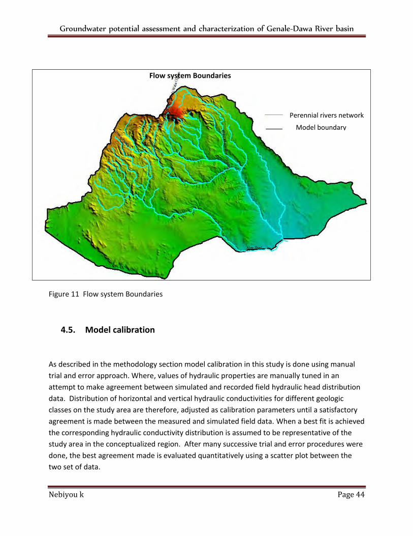
Groundwater potential assessment and characterization of Genale-Dawa River basin
Nebiyou k Page 44
Figure 11 Flow system Boundaries
4.5. Model calibration
As described in the methodology section model calibration in this study is done using manual
trial and error approach. Where, values of hydraulic properties are manually tuned in an
attempt to make agreement between simulated and recorded field hydraulic head distribution
data. Distribution of horizontal and vertical hydraulic conductivities for different geologic
classes on the study area are therefore, adjusted as calibration parameters until a satisfactory
agreement is made between the measured and simulated field data. When a best fit is achieved
the corresponding hydraulic conductivity distribution is assumed to be representative of the
study area in the conceptualized region. After many successive trial and error procedures were
done, the best agreement made is evaluated quantitatively using a scatter plot between the
two set of data.
Perennial rivers network
Model boundary
Flow system Boundaries
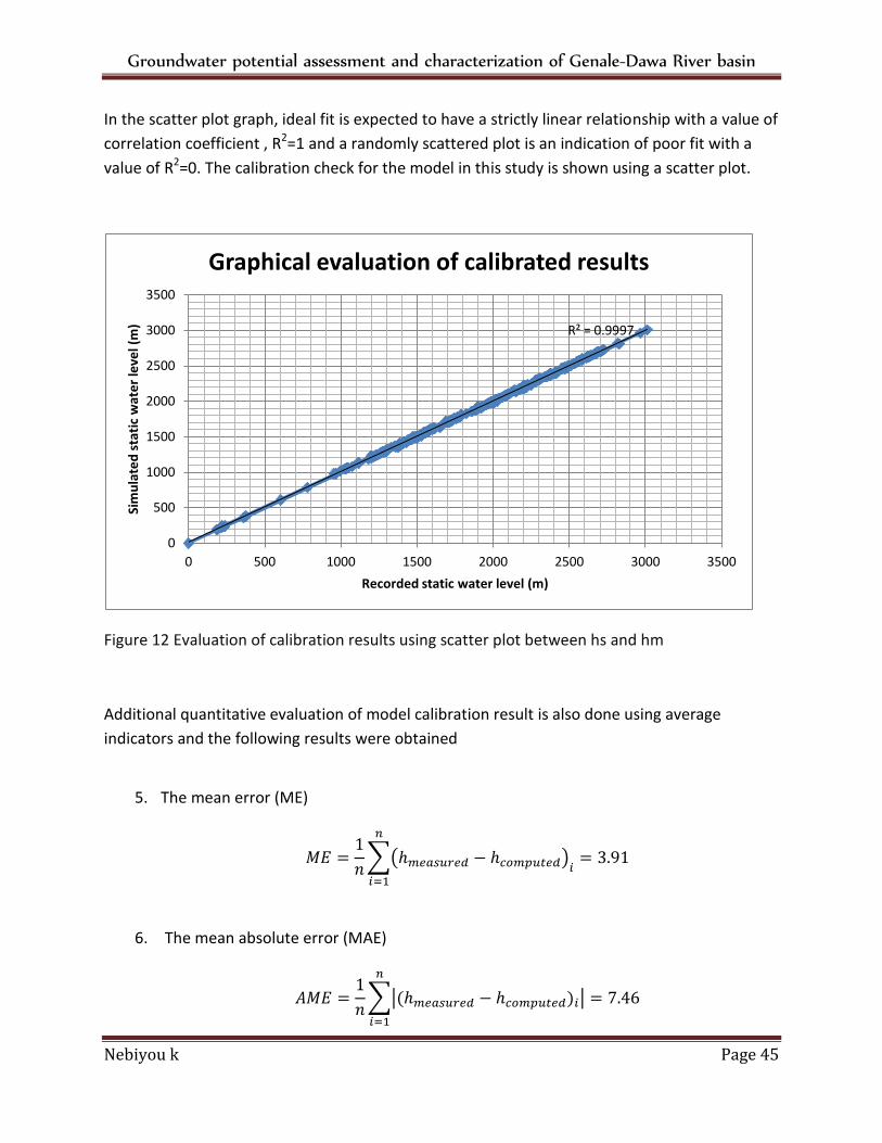
Groundwater potential assessment and characterization of Genale-Dawa River basin
Nebiyou k Page 45
In the scatter plot graph, ideal fit is expected to have a strictly linear relationship with a value of
correlation coefficient , R2=1 and a randomly scattered plot is an indication of poor fit with a
value of R2=0. The calibration check for the model in this study is shown using a scatter plot.
Figure 12 Evaluation of calibration results using scatter plot between hs and hm
Additional quantitative evaluation of model calibration result is also done using average
indicators and the following results were obtained
5. The mean error (ME)
6. The mean absolute error (MAE)
R² = 0.9997
0
500
1000
1500
2000
2500
3000
3500
0 500 1000 1500 2000 2500 3000 3500
Sim
ula
ted
sta
tic
wat
er
leve
l (m
)
Recorded static water level (m)
Graphical evaluation of calibrated results
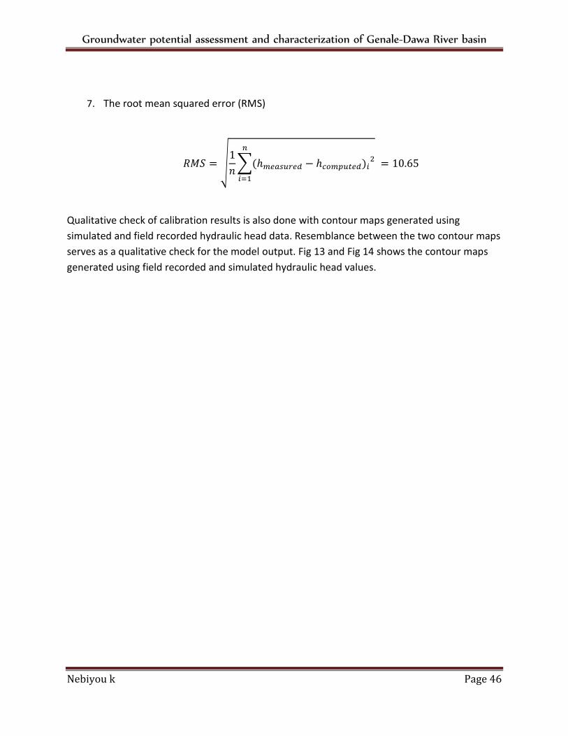
Groundwater potential assessment and characterization of Genale-Dawa River basin
Nebiyou k Page 46
7. The root mean squared error (RMS)
Qualitative check of calibration results is also done with contour maps generated using
simulated and field recorded hydraulic head data. Resemblance between the two contour maps
serves as a qualitative check for the model output. Fig 13 and Fig 14 shows the contour maps
generated using field recorded and simulated hydraulic head values.
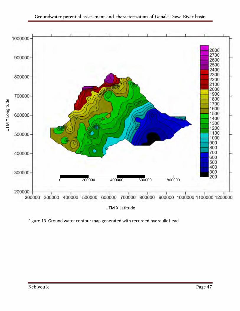
Groundwater potential assessment and characterization of Genale-Dawa River basin
Nebiyou k Page 47
Figure 13 Ground water contour map generated with recorded hydraulic head
UTM X Latitude
UTM
Y L
on
gitu
de
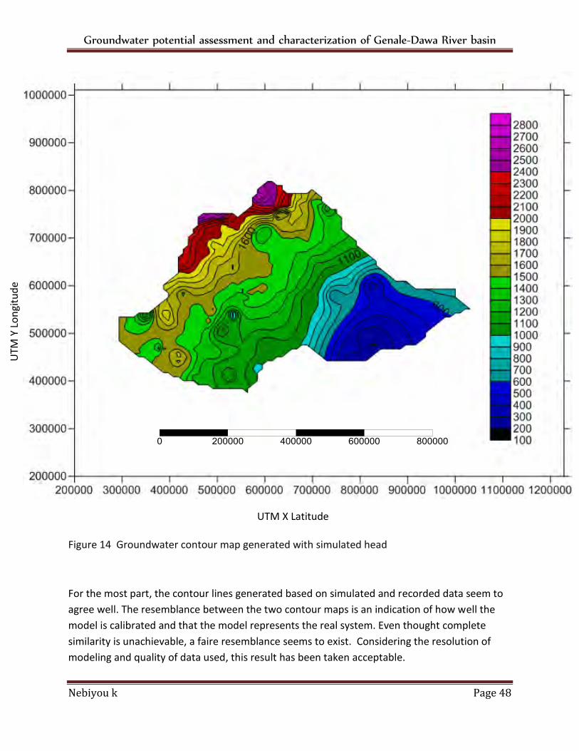
Groundwater potential assessment and characterization of Genale-Dawa River basin
Nebiyou k Page 48
Figure 14 Groundwater contour map generated with simulated head
For the most part, the contour lines generated based on simulated and recorded data seem to
agree well. The resemblance between the two contour maps is an indication of how well the
model is calibrated and that the model represents the real system. Even thought complete
similarity is unachievable, a faire resemblance seems to exist. Considering the resolution of
modeling and quality of data used, this result has been taken acceptable.
UTM X Latitude
UTM
Y L
on
gitu
de
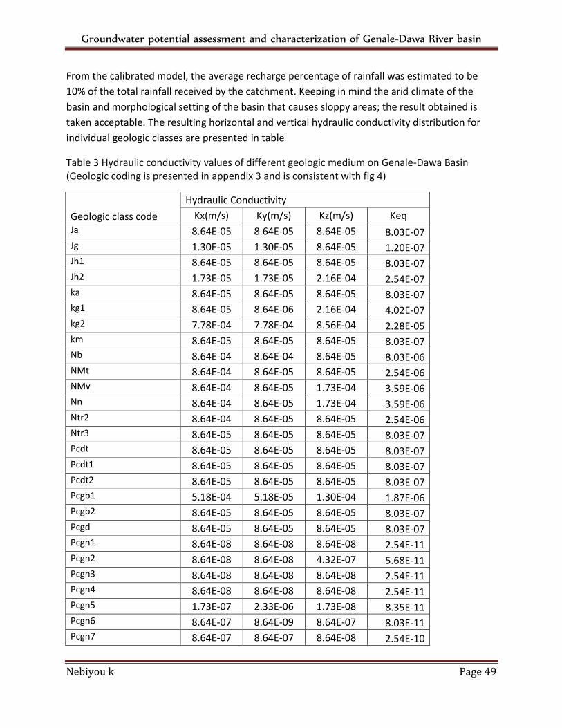
Groundwater potential assessment and characterization of Genale-Dawa River basin
Nebiyou k Page 49
From the calibrated model, the average recharge percentage of rainfall was estimated to be
10% of the total rainfall received by the catchment. Keeping in mind the arid climate of the
basin and morphological setting of the basin that causes sloppy areas; the result obtained is
taken acceptable. The resulting horizontal and vertical hydraulic conductivity distribution for
individual geologic classes are presented in table
Table 3 Hydraulic conductivity values of different geologic medium on Genale-Dawa Basin (Geologic coding is presented in appendix 3 and is consistent with fig 4)
Geologic class code
Hydraulic Conductivity
Kx(m/s) Ky(m/s) Kz(m/s) Keq
Ja 8.64E-05 8.64E-05 8.64E-05 8.03E-07 Jg 1.30E-05 1.30E-05 8.64E-05 1.20E-07 Jh1 8.64E-05 8.64E-05 8.64E-05 8.03E-07 Jh2 1.73E-05 1.73E-05 2.16E-04 2.54E-07 ka 8.64E-05 8.64E-05 8.64E-05 8.03E-07 kg1 8.64E-05 8.64E-06 2.16E-04 4.02E-07 kg2 7.78E-04 7.78E-04 8.56E-04 2.28E-05 km 8.64E-05 8.64E-05 8.64E-05 8.03E-07 Nb 8.64E-04 8.64E-04 8.64E-05 8.03E-06 NMt 8.64E-04 8.64E-05 8.64E-05 2.54E-06 NMv 8.64E-04 8.64E-05 1.73E-04 3.59E-06 Nn 8.64E-04 8.64E-05 1.73E-04 3.59E-06 Ntr2 8.64E-04 8.64E-05 8.64E-05 2.54E-06 Ntr3 8.64E-05 8.64E-05 8.64E-05 8.03E-07 Pcdt 8.64E-05 8.64E-05 8.64E-05 8.03E-07 Pcdt1 8.64E-05 8.64E-05 8.64E-05 8.03E-07 Pcdt2 8.64E-05 8.64E-05 8.64E-05 8.03E-07 Pcgb1 5.18E-04 5.18E-05 1.30E-04 1.87E-06 Pcgb2 8.64E-05 8.64E-05 8.64E-05 8.03E-07 Pcgd 8.64E-05 8.64E-05 8.64E-05 8.03E-07 Pcgn1 8.64E-08 8.64E-08 8.64E-08 2.54E-11 Pcgn2 8.64E-08 8.64E-08 4.32E-07 5.68E-11 Pcgn3 8.64E-08 8.64E-08 8.64E-08 2.54E-11 Pcgn4 8.64E-08 8.64E-08 8.64E-08 2.54E-11 Pcgn5 1.73E-07 2.33E-06 1.73E-08 8.35E-11 Pcgn6 8.64E-07 8.64E-09 8.64E-07 8.03E-11 Pcgn7 8.64E-07 8.64E-07 8.64E-08 2.54E-10
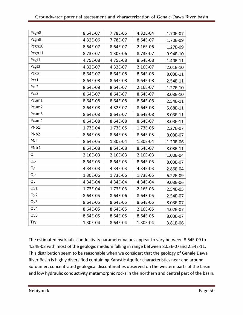
Groundwater potential assessment and characterization of Genale-Dawa River basin
Nebiyou k Page 50
Pcgn8 8.64E-07 7.78E-05 4.32E-04 1.70E-07 Pcgn9 4.32E-06 7.78E-07 8.64E-07 1.70E-09 Pcgn10 8.64E-07 8.64E-07 2.16E-06 1.27E-09 Pcgn11 8.73E-07 1.30E-06 8.73E-07 9.94E-10 Pcgt1 4.75E-08 4.75E-08 8.64E-08 1.40E-11 Pcgt2 4.32E-07 4.32E-07 2.16E-07 2.01E-10 Pckb 8.64E-07 8.64E-08 8.64E-08 8.03E-11 Pcs1 8.64E-08 8.64E-08 8.64E-08 2.54E-11 Pcs2 8.64E-08 8.64E-07 2.16E-07 1.27E-10 Pcs3 8.64E-07 8.64E-07 8.64E-07 8.03E-10 Pcum1 8.64E-08 8.64E-08 8.64E-08 2.54E-11 Pcum2 8.64E-08 4.32E-07 8.64E-08 5.68E-11 Pcum3 8.64E-08 8.64E-07 8.64E-08 8.03E-11 Pcum4 8.64E-08 8.64E-08 8.64E-07 8.03E-11 PNb1 1.73E-04 1.73E-05 1.73E-05 2.27E-07 PNb2 8.64E-05 8.64E-05 8.64E-05 8.03E-07 PNi 8.64E-05 1.30E-04 1.30E-04 1.20E-06 PNtr1 8.64E-08 8.64E-08 8.64E-07 8.03E-11 Q 2.16E-03 2.16E-03 2.16E-03 1.00E-04 Q6 8.64E-05 8.64E-05 8.64E-05 8.03E-07 Qa 4.34E-03 4.34E-03 4.34E-03 2.86E-04 Qe 1.30E-06 1.73E-06 1.73E-05 6.22E-09 Qv 4.34E-04 4.34E-04 4.34E-04 9.03E-06 Qv1 1.73E-04 1.73E-03 2.16E-03 2.54E-05 Qv2 8.64E-05 8.64E-06 8.64E-05 2.54E-07 Qv3 8.64E-05 8.64E-05 8.64E-05 8.03E-07 Qv4 8.64E-05 8.64E-05 2.16E-05 4.02E-07 Qv5 8.64E-05 8.64E-05 8.64E-05 8.03E-07 Tsy 1.30E-04 8.64E-04 1.30E-04 3.81E-06
The estimated hydraulic conductivity parameter values appear to vary between 8.64E-09 to
4.34E-03 with most of the geologic medium falling in range between 8.03E-07and 2.54E-11.
This distribution seem to be reasonable when we consider; that the geology of Genale Dawa
River Basin is highly diversified containing Karastic Aquifer characteristics near and around
Sofoumer, concentrated geological discontinuities observed on the western parts of the basin
and low hydraulic conductivity metamorphic rocks in the northern and central part of the basin.
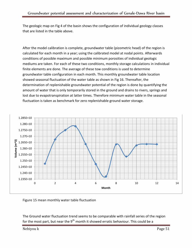
Groundwater potential assessment and characterization of Genale-Dawa River basin
Nebiyou k Page 51
The geologic map on Fig 4 of the basin shows the configuration of individual geology classes
that are listed in the table above.
After the model calibration is complete, groundwater table (pizometric head) of the region is
calculated for each month in a year; using the calibrated model at nodal points. Afterwards
conditions of possible maximum and possible minimum porosities of individual geologic
mediums are taken. For each of these two conditions, monthly storage calculations in individual
finite elements are done. The average of these tow conditions is used to determine
groundwater table configuration in each month. This monthly groundwater table location
showed seasonal fluctuation of the water table as shown in Fig 16. Thereafter, the
determination of replenishable groundwater potential of the region is done by quantifying the
amount of water that is only temporarily stored in the ground and drains to rivers, springs and
lost due to evapotranspiration at latter times. Therefore minimum water table in the seasonal
fluctuation is taken as benchmark for zero replenishable ground water storage.
Figure 15 mean monthly water table fluctuation
The Ground water fluctuation trend seems to be comparable with rainfall series of the region
for the most part, but near the 9th month it showed erratic behaviour. This could be a
1.235E+10
1.24E+10
1.245E+10
1.25E+10
1.255E+10
1.26E+10
1.265E+10
1.27E+10
1.275E+10
1.28E+10
1.285E+10
0 2 4 6 8 10 12 14
Vo
lum
e (
m^3
)
Month

Groundwater potential assessment and characterization of Genale-Dawa River basin
Nebiyou k Page 52
cumulative result of a very complex geologic composition of the region and spatially non
uniform rainfall pattern in the region.
In order to determine the total replenishable ground water reserve, monthly contribution of
groundwater to rivers shall also be taken in to account. Accordingly base flow separation of
stream flow data was done using single parameter digital filter approach (Appendix 1) and the
result was added to the volume of replenishable ground water obtained from the model. This
has resulted in 2.78BM3 as total replenishable groundwater in Genale Dawa basin; the result is
shown in table below.
Table 4 Total Replenishable Ground Water Calculation
Month
Replenishable Ground Water (M3)
Base flow contribution to rivers(M3)
Total monthly Replenishable Ground Water (M3)
jan 1.05E+08 2.74E+03 1.05E+08
Feb 3.03E+08 2.65E+03 3.03E+08
mar 3.79E+08 3.20E+03 3.79E+08
apr 4.11E+08 4.35E+03 4.11E+08
may 2.65E+08 6.18E+03 2.65E+08
jun 1.02E+08 5.90E+03 1.02E+08
jul 0.00E+00 8.52E+03 8.52E+03
aug 2.63E+08 9.67E+03 2.63E+08
sep 1.63E+08 1.43E+04 1.63E+08
oct 2.54E+08 1.59E+04 2.54E+08
nov 2.65E+08 2.69E+04 2.65E+08
dec 2.64E+08 2.61E+04 2.64E+08
Total Replenishable Ground Water 2.78E+09
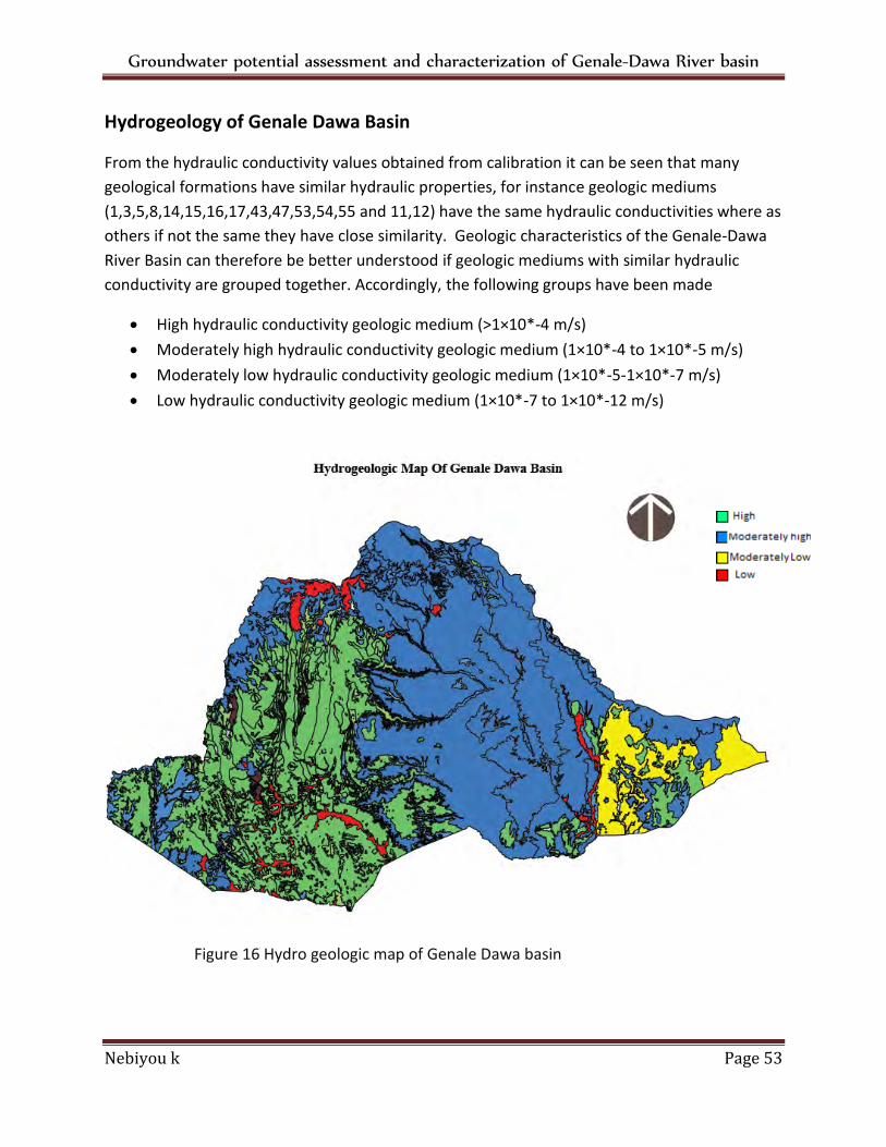
Groundwater potential assessment and characterization of Genale-Dawa River basin
Nebiyou k Page 53
Hydrogeology of Genale Dawa Basin
From the hydraulic conductivity values obtained from calibration it can be seen that many
geological formations have similar hydraulic properties, for instance geologic mediums
(1,3,5,8,14,15,16,17,43,47,53,54,55 and 11,12) have the same hydraulic conductivities where as
others if not the same they have close similarity. Geologic characteristics of the Genale-Dawa
River Basin can therefore be better understood if geologic mediums with similar hydraulic
conductivity are grouped together. Accordingly, the following groups have been made
High hydraulic conductivity geologic medium (>1×10*-4 m/s)
Moderately high hydraulic conductivity geologic medium (1×10*-4 to 1×10*-5 m/s)
Moderately low hydraulic conductivity geologic medium (1×10*-5-1×10*-7 m/s)
Low hydraulic conductivity geologic medium (1×10*-7 to 1×10*-12 m/s)
Figure 16 Hydro geologic map of Genale Dawa basin
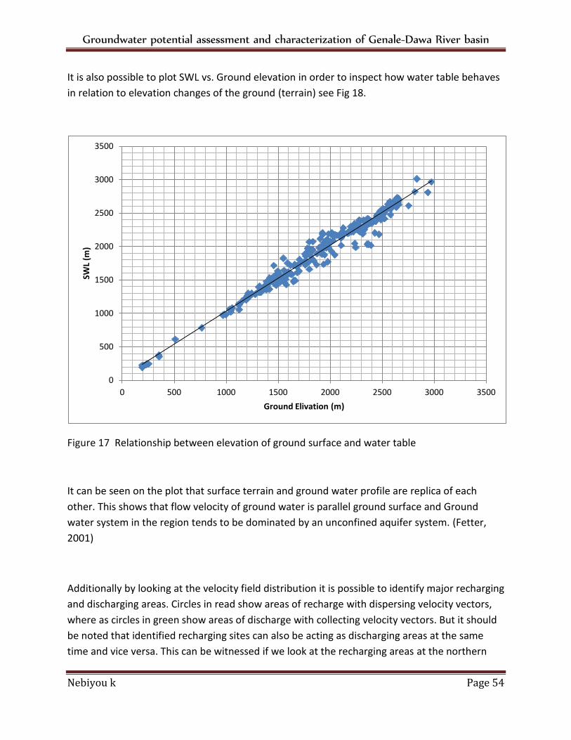
Groundwater potential assessment and characterization of Genale-Dawa River basin
Nebiyou k Page 54
It is also possible to plot SWL vs. Ground elevation in order to inspect how water table behaves
in relation to elevation changes of the ground (terrain) see Fig 18.
Figure 17 Relationship between elevation of ground surface and water table
It can be seen on the plot that surface terrain and ground water profile are replica of each
other. This shows that flow velocity of ground water is parallel ground surface and Ground
water system in the region tends to be dominated by an unconfined aquifer system. (Fetter,
2001)
Additionally by looking at the velocity field distribution it is possible to identify major recharging
and discharging areas. Circles in read show areas of recharge with dispersing velocity vectors,
where as circles in green show areas of discharge with collecting velocity vectors. But it should
be noted that identified recharging sites can also be acting as discharging areas at the same
time and vice versa. This can be witnessed if we look at the recharging areas at the northern
0
500
1000
1500
2000
2500
3000
3500
0 500 1000 1500 2000 2500 3000 3500
SWL
(m)
Ground Elivation (m)
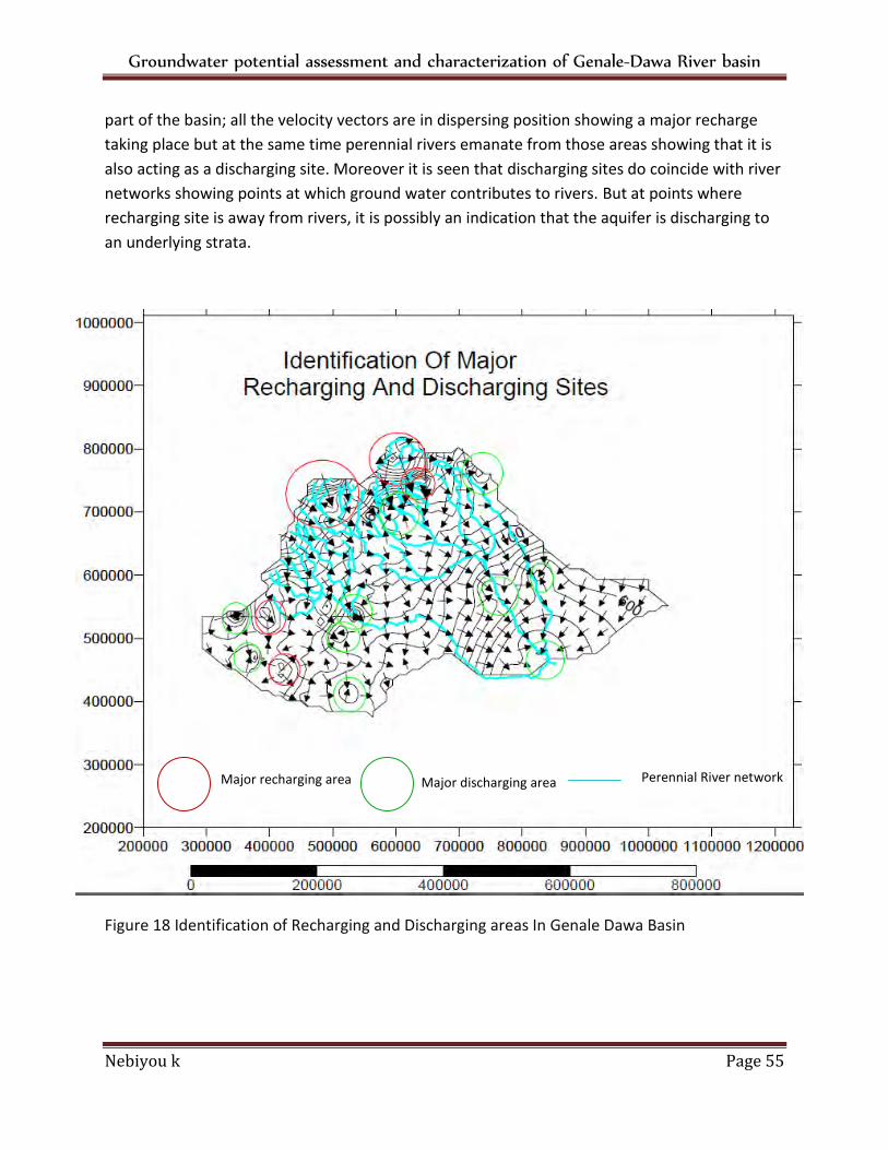
Groundwater potential assessment and characterization of Genale-Dawa River basin
Nebiyou k Page 55
part of the basin; all the velocity vectors are in dispersing position showing a major recharge
taking place but at the same time perennial rivers emanate from those areas showing that it is
also acting as a discharging site. Moreover it is seen that discharging sites do coincide with river
networks showing points at which ground water contributes to rivers. But at points where
recharging site is away from rivers, it is possibly an indication that the aquifer is discharging to
an underlying strata.
Figure 18 Identification of Recharging and Discharging areas In Genale Dawa Basin
Major recharging area Major discharging area Perennial River network
Groundwater potential assessment and characterization of Genale-Dawa River basin
Nebiyou k Page 56
5. Conclusion and Recommendation
5.1. Conclusion
Groundwater modeling has versatile applications in groundwater resources management that
can be used for groundwater pollution management and more. This study used finite element
based three dimensional groundwater modeling program called TAGSAC to estimate the
groundwater recharge potential as described in the previous chapters. The findings of this
research showed that the basin has an average recharging potential of 2.78 BCM. This is in
order with previous estimations made by WAPCOS in 1990 which was 0.433BCM using recharge
area approach. But considering that recent data have also been incorporated in this study and
that a different methodology has been employed, the result can be taken as a good estimation.
An improved delineation has also been used that helps in making better estimate. However,
further study on estimation of extraction factor shall be done. This factor accounts for the
sociological, botaniuque and other concerned factors to determine the safest amount of
groundwater that can be extracted from the basin. In addition, this study also attempted to
characterize the groundwater flow system of the basin by preparing hydro-geological map and
contour map, which can be useful in selection of well field in the future.
It should also be noted that this study has faced some challenges due to limitations in
computational resources. This has restricted the model not to use finer finite element sizes
which would have a positive effect towards better ground water potential estimate. The luck in
availability of detailed geological data has also limited the model with a single layer that
represents the aquifer system in the vertical extent. With detailed geological investigation an
improved model with multiple layers can be developed. Therefore, future studies on the basin
can improve on these to get a better estimation.
Groundwater potential assessment and characterization of Genale-Dawa River basin
Nebiyou k Page 57
5.2. Recommendation
Based on the results obtained from the study the following recommendations are forwarded;
The identified sites of recharge area shall be protected from polluting chemicals to
assure quality of the regions groundwater. Forestation of this area can also increase the
available groundwater reserve by increasing the amount of infiltration and percolation
hence; it is recommended to plane and execute environmental protection projects in
these regions.
Identified discharging areas can be used as well fields after carrying out the necessary
detail investigation on the site. Therefore the regional authorities can consider ground
water based water supply schemes for domestic and industrial purposes.
Regular well monitoring shall be planned and executed in the region to gather better
quality data and widen our understanding of the basins groundwater flow system which
can be used as an input for future study. Concerned authorities shall also provide a
framework that can enforce the collection and report of well inventory data including
geological log, time log and other standard records at the time of well drillings and
completion.
Groundwater potential assessment and characterization of Genale-Dawa River basin
Nebiyou k Page 58
Reference
Aklilu, & Hilu. (2001). Groundwater resource assessment core process.
Alemayehu, T. (2006). Ground water occurrence in Ethiopia.
Anderson, M. p., & Woessner, W. W. (1992). Applied Ground water modeling simulation of flow
and advective transport .
Anderson, M. P., & Wosner, W. W. (1992). Applied Grounwater Modeling; Simulation of Flow
and Advictive Transport. sen dieago, New York, Boston: Accadamic press.
ASTEM. (2008). Standard Guide for Calibrating a Groundwater Flow Model Application1 D5981
– 96.
Beyene, A., Nigussie, Y., & Tesema, Z. (1987). Hydro-geology of upper Dawa basin mainly based
on land sate interpretation.
Charles R., F., & Mercer, J. w. (2006). Groundwater modeling: Numerical models .
Delleur, J. (1999). The hand book of ground water engineering, . School of Civil Engineering
Purdue University West Lafayette, Indiana.
Diodato, D. (1994). A Compendium of Fracture Flow Models.
Essink, G. O. (2000, September). ground water modeling. L4018/GWMI/Utrecht University .
Ethiopian National Meteorological Agency. (2013). Hydro Meteorological Bulletin for May .
Faust, C. R., & Mercer, J. W. (2006). Groundwater modeling: numerical model.
Fetter, C. W. (2001). Applied Hydrogeology. New Jersey: prentice-Hall.
fitts, C. R. (2002). Groundwater science. Amsterdam, Sidney, London: Accadamic press.
Hailemariam, A. ( 1990). report on regional and detailed geophysical surveys in moyale area,
sidamo EIGS.
Healy, R. W. (2010). Estimating Groundwater Recharge.
Herbert F Wang, m. p. (1982). Introduction to ground water modeling, finite difference and
finite element methods.
Groundwater potential assessment and characterization of Genale-Dawa River basin
Nebiyou k Page 59
Istoke, J. I. (1989). Groundwater Modeling, by the Finite Element Method.
Kemper. ( 2004). Groundwater from development to management : hydrogeology journal
theme issue : Groundwater from development to management : hydrogeology journal theme
issue 12(1) (English).
kiflu, A., tafa, y., & mulugeta, y. (2001). Ministry of Mines and Energy Geological Survey of
Ethiopia.
Kresic, N. (2009). Hydrology and groundwater modeling Groundwater resource. London, New
York: CRC press.
Mab consult – consulting hydro-geologists, a. e. (2007). GROUNDWATER POTENTIAL ZONE
MAPPING USING GIS AND REMOTE SENSING - MOYALE-TELTELE SUB BASIN - DIRE, ARERO,
YABELO AND TELTELE WOREDAS, BORENA ZONE OF OROMIA REGIONAL STATE.
Moges, S. (2012). (AgWater Solutions Project Case StudyAgricultural Use of Ground Water in
Ethiopia: Assessment of Potential and Analysis of Economics, Policies, Constraints and
Opportunities.
Mohammed, M. (2010). Adaptive NEuro Fuzzy In ference System Approach For Prediction of
Hydraulic Pressure Recharge.
Moore, & Wilson. (1998). Glossary of hydrology.
MOWR. (2007). Genale Dawa River basin intigrated resources development master plan study,
Geology sector.
MOWR. (2007). Genale Dawa River basin intigrated resources development master plan study,
hydrology sector,.
MOWR. (2007). Genale Dawa River basin intigrated resources development master plan study.
MOWR. (2007). Genale Dawa River basin intigrated resources development master plan study
hydro-Geology sector.
MOWR. (2007). Genale Dawa River basin intigrated resources development master plan study
hydrology sector.
MOWR. (2007). Genale Dawa River basin intigrated resources development master plan study
hydrology sector.
Groundwater potential assessment and characterization of Genale-Dawa River basin
Nebiyou k Page 60
MOWR. (2007). Genale-Dawa River Basin Integrated Resources Development Master Plan
Study.
MOWR. (2007). Integrated River Basin Master Plan Studies, carrried out during.
prickett. (1975). Introduction to ground water modeling.
Rao, S. S. (2005). Finite element method in engineering, .
Reilly, T. E. (2001). USGS Book 3, System and Boundary Conceptualization in Ground-Water
Flow Simulation .
Sarkar, S., Toksöz, M. N., & Burns, D. R. (n.d.). Fluid Flow Simulation in Fractured Reservoirs.
Semu. (2012). Ag Water solution project, case study.
Thangarajan. (2007). Groundwater, Resource Evaluation, Augmentation, Contamination,
Restoration, Modeling and Management.
Thangarajan. (2007). Groundwater, Resource Evaluation, Augmentation,
Contamination,Restoration, Modeling and Management.
Vries, d., & Simmer. (2000).
WAPCOS, S. B. (2007). Water Resource and Irrigation Development in Ethiopia.
Zehang, Y. ( 2011). Groundwater Flow and Solute Transport Modeling.
Groundwater potential assessment and characterization of Genale-Dawa River basin
Nebiyou k Page 61
Appendix 1 Continuous Base flow Separation Method
Digital filter is a frequency analysis method initially developed for signal analysis. Now days it is
widely applicable for base flow separation in Hydrology
Approach:
Use a numerical algorithm (a digital filter) to partition the streamflow hydrograph into “high
frequency” (direct runoff) and “low frequency” (baseflow) components. One type of digital
filter approach is show as follows. (Nathan and McMahon, 1990)
Terms:
Qk streamflow at time step k
Rk direct runoff at time step k
Bk baseflow at time step k
Parameter:
α base flow filter parameter, it’s an attenuation coefficient between 0.9 and 0.995. The bigger
the attenuation the stronger the runoff, and the lesser the base flow a value of 0.95 was used
for this study.
Algorithm:
At each time step:
Check:
If <0 then =0
If >then =
Compute base Flow:
Groundwater potential assessment and characterization of Genale-Dawa River basin
Nebiyou k Page 62
= -
Appendix 2 Water point calibration data
No. TYPE
SITE_NAME REGION ZONE WEREDA UTM_X UTM_Y SWL
1 BH Ali Town No 1 OROMIYA
BALE Agarfa 603061
800340
10
2 BH Ginir OROMIYA
BALE Ginir 690000
788000
12
3 BH Melka Oda OROMIYA
BALE Ginir 695164
774045
8.25
4 BH Melka Oda OROMIYA
BALE Ginir 703398
775701
22
5 BH Melka Oda No. 1 OROMIYA
BALE Ginir 705143
773469
12
6 BH Tullicha No 3 OROMIYA
BALE Ginir 700224
779151
21
7 BH Melka Buta OROMIYA
BALE Goro 678614
766613
8
8 BH Sinana No 3 State Farm OROMIYA
BALE Goro 643010
778424
69
9 BH Abasirba No 1 OROMIYA
BALE Meda Welabu
582087
650554
5
10 BH Abasirba No 2 OROMIYA
BALE Meda Welabu
581677
650904
16
11 BH Bidire BH5 OROMIYA
BALE Meda Welabu
572126
653662
15
12 BH Bidire No 1 OROMIYA
BALE Meda Welabu
572528
654484
8
13 BH Bidire town No 2 OROMIYA
BALE Meda Welabu
571808
654328
8
14 BH Bidire town No 3 OROMIYA
BALE Meda Welabu
570757
654018
13
15 BH Elabidire No 1 OROMIYA
BALE Meda Welabu
574483
652798
8
16 BH Elabidire No 2 OROMIYA
BALE Meda Welabu
576094
652237
17
17 BH Meda No 1 OROMIYA
BALE Meda Welabu
598530
643569
6
18 BH Meda No 2 OROMIYA
BALE Meda Welabu
598282
643752
9
19 BH Oborso No 2 OROMIYA
BALE Meda Welabu
544465
678347
21
20 BH Oda OROMIYA
BALE Meda Welabu
551274
672099
8
21 BH Burkitu Derara No 1 OROMIYA
BALE Mena Angetu
593846
712069
13
22 BH Chiri Harewa No 1 OROMIYA
BALE Mena Angetu
586194
708130
18
23 BH Chiri Harewa No 2 OROMIYA
BALE Mena Angetu
586613
708315
12
24 BH Dayu Harewa WELL NO 3 OROMIYA
BALE Mena Angetu
607515
717509
16
25 BH Erba No 1 OROMIYA
BALE Mena Angetu
596078
713394
12
26 BH Erba No 2 OROMIYA
BALE Mena Angetu
596544
713706
15.36
27 BH Gomgoma No 1 OROMIYA
BALE Mena Angetu
592601
698164
8
28 BH Mena town BH4 OROMIYA
BALE Mena Angetu
594924
708629
6
29 BH Weltai Gudina No 1 OROMIYA
BALE Mena Angetu
601339
715590
14
30 BH Weltai Gudina No 2 OROMIYA
BALE Mena Angetu
601866
716191
13
31 BH Chelchel No 1 OROMIYA
BALE Rayitu 729188
763589
17
32 BH Chelchel No 2 OROMIYA
BALE Rayitu 729099
763783
15
33 BH Bale Robe Airport OROMIYA
BALE Sinanana Dinsho
614635
786982
11.25
34 BH Robe Catholic School OROMIYA
BALE Sinanana Dinsho
610824
784977
5
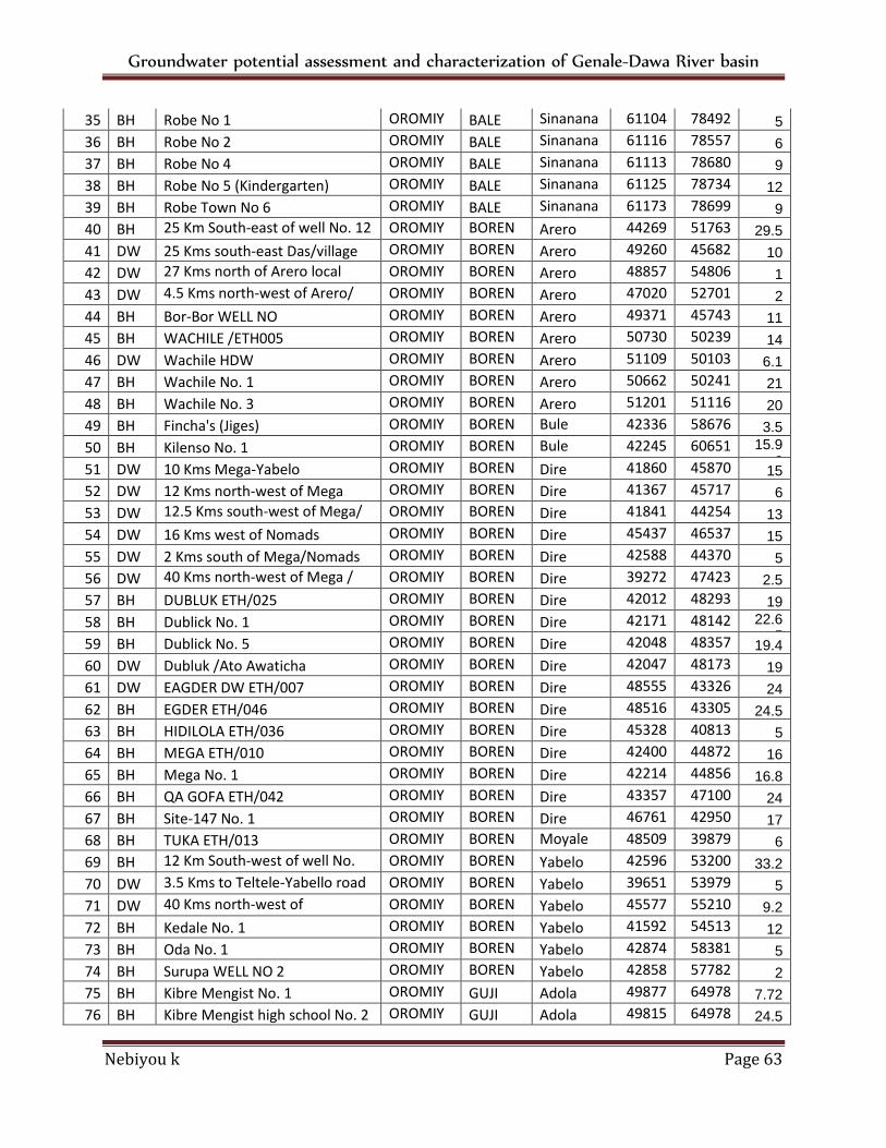
Groundwater potential assessment and characterization of Genale-Dawa River basin
Nebiyou k Page 63
35 BH Robe No 1 OROMIYA
BALE Sinanana Dinsho
611048
784924
5
36 BH Robe No 2 OROMIYA
BALE Sinanana Dinsho
611162
785579
6
37 BH Robe No 4 OROMIYA
BALE Sinanana Dinsho
611139
786804
9
38 BH Robe No 5 (Kindergarten) OROMIYA
BALE Sinanana Dinsho
611254
787346
12
39 BH Robe Town No 6 OROMIYA
BALE Sinanana Dinsho
611730
786993
9
40 BH 25 Km South-east of well No. 12 /NCA
OROMIYA
BORENA
Arero 442697
517634
29.5
41 DW 25 Kms south-east Das/village OROMIYA
BORENA
Arero 492601
456824
10
42 DW 27 Kms north of Arero local nomads
OROMIYA
BORENA
Arero 488572
548067
1
43 DW 4.5 Kms north-west of Arero/ village
OROMIYA
BORENA
Arero 470209
527012
2
44 BH Bor-Bor WELL NO OROMIYA
BORENA
Arero 493711
457438
11
45 BH WACHILE /ETH005 OROMIYA
BORENA
Arero 507302
502396
14
46 DW Wachile HDW OROMIYA
BORENA
Arero 511093
501035
6.1
47 BH Wachile No. 1 OROMIYA
BORENA
Arero 506625
502416
21
48 BH Wachile No. 3 OROMIYA
BORENA
Arero 512016
511167
20
49 BH Fincha's (Jiges) OROMIYA
BORENA
Bule Hora
423360
586767
3.5
50 BH Kilenso No. 1 OROMIYA
BORENA
Bule Hora
422459
606511
15.92
51 DW 10 Kms Mega-Yabelo OROMIYA
BORENA
Dire 418607
458703
15
52 DW 12 Kms north-west of Mega OROMIYA
BORENA
Dire 413673
457173
6
53 DW 12.5 Kms south-west of Mega/ Nomads
OROMIYA
BORENA
Dire 418416
442547
13
54 DW 16 Kms west of Nomads OROMIYA
BORENA
Dire 454375
465371
15
55 DW 2 Kms south of Mega/Nomads OROMIYA
BORENA
Dire 425885
443701
5
56 DW 40 Kms north-west of Mega / Nomads
OROMIYA
BORENA
Dire 392727
474238
2.5
57 BH DUBLUK ETH/025 OROMIYA
BORENA
Dire 420123
482935
19
58 BH Dublick No. 1 OROMIYA
BORENA
Dire 421711
481421
22.65
59 BH Dublick No. 5 OROMIYA
BORENA
Dire 420480
483572
19.4
60 DW Dubluk /Ato Awaticha OROMIYA
BORENA
Dire 420479
481730
19
61 DW EAGDER DW ETH/007 OROMIYA
BORENA
Dire 485558
433264
24
62 BH EGDER ETH/046 OROMIYA
BORENA
Dire 485160
433051
24.5
63 BH HIDILOLA ETH/036 OROMIYA
BORENA
Dire 453285
408132
5
64 BH MEGA ETH/010 OROMIYA
BORENA
Dire 424006
448721
16
65 BH Mega No. 1 OROMIYA
BORENA
Dire 422144
448568
16.8
66 BH QA GOFA ETH/042 OROMIYA
BORENA
Dire 433572
471000
24
67 BH Site-147 No. 1 OROMIYA
BORENA
Dire 467618
429505
17
68 BH TUKA ETH/013 OROMIYA
BORENA
Moyale (OR)
485094
398799
6
69 BH 12 Km South-west of well No. 11 Ministry of agriculture
OROMIYA
BORENA
Yabelo 425969
532006
33.2
70 DW 3.5 Kms to Teltele-Yabello road / village
OROMIYA
BORENA
Yabelo 396511
539790
5
71 DW 40 Kms north-west of Arero/local nomads
OROMIYA
BORENA
Yabelo 455775
552104
9.2
72 BH Kedale No. 1 OROMIYA
BORENA
Yabelo 415923
545139
12
73 BH Oda No. 1 OROMIYA
BORENA
Yabelo 428743
583813
5
74 BH Surupa WELL NO 2 OROMIYA
BORENA
Yabelo 428583
577826
2
75 BH Kibre Mengist No. 1 OROMIYA
GUJI Adola 498770
649788
7.72
76 BH Kibre Mengist high school No. 2 OROMIYA
GUJI Adola 498153
649788
24.5
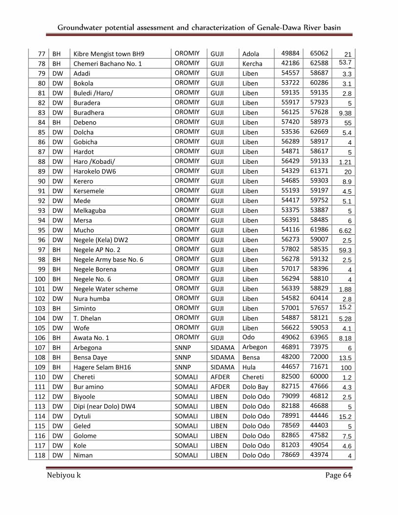
Groundwater potential assessment and characterization of Genale-Dawa River basin
Nebiyou k Page 64
77 BH Kibre Mengist town BH9 OROMIYA
GUJI Adola 498847
650620
21
78 BH Chemeri Bachano No. 1 OROMIYA
GUJI Kercha 421867
625887
53.75
79 DW Adadi OROMIYA
GUJI Liben 545577
586870
3.3
80 DW Bokola OROMIYA
GUJI Liben 537220
602868
3.1
81 DW Buledi /Haro/ OROMIYA
GUJI Liben 591351
591351
2.8
82 DW Buradera OROMIYA
GUJI Liben 559176
579236
5
83 DW Buradhera OROMIYA
GUJI Liben 561253
576286
9.38
84 BH Debeno OROMIYA
GUJI Liben 574204
589737
55
85 DW Dolcha OROMIYA
GUJI Liben 535365
626696
5.4
86 DW Gobicha OROMIYA
GUJI Liben 562892
589178
4
87 DW Hardot OROMIYA
GUJI Liben 548711
586172
5
88 DW Haro /Kobadi/ OROMIYA
GUJI Liben 564297
591332
1.21
89 DW Harokelo DW6 OROMIYA
GUJI Liben 543295
613714
20
90 DW Kerero OROMIYA
GUJI Liben 546856
593039
8.9
91 DW Kersemele OROMIYA
GUJI Liben 551934
591970
4.5
92 DW Mede OROMIYA
GUJI Liben 544173
597521
5.1
93 DW Melkaguba OROMIYA
GUJI Liben 533758
538878
5
94 DW Mersa OROMIYA
GUJI Liben 563915
584857
6
95 DW Mucho OROMIYA
GUJI Liben 541167
619863
6.62
96 DW Negele (Kela) DW2 OROMIYA
GUJI Liben 562739
590079
2.5
97 BH Negele AP No. 2 OROMIYA
GUJI Liben 578027
585356
59.3
98 BH Negele Army base No. 6 OROMIYA
GUJI Liben 562785
591328
2.5
99 BH Negele Borena OROMIYA
GUJI Liben 570179
583966
4
100 BH Negele No. 6 OROMIYA
GUJI Liben 562942
588104
4
101 DW Negele Water scheme OROMIYA
GUJI Liben 563390
588292
1.88
102 DW Nura humba OROMIYA
GUJI Liben 545829
604140
2.8
103 BH Siminto OROMIYA
GUJI Liben 570013
576574
15.25
104 DW T. Dhelan OROMIYA
GUJI Liben 548871
581210
5.28
105 DW Wofe OROMIYA
GUJI Liben 566227
590533
4.1
106 BH Awata No. 1 OROMIYA
GUJI Odo Shakiso
490620
639656
8.18
107 BH Arbegona SNNP SIDAMA Arbegona
468912
739750
6
108 BH Bensa Daye SNNP SIDAMA Bensa 482000
720000
13.5
109 BH Hagere Selam BH16 SNNP SIDAMA Hula 446577
716715
100
110 DW Chereti SOMALI AFDER Chereti 825000
600000
1.2
111 DW Bur amino SOMALI AFDER Dolo Bay 827155
476669
4.3
112 DW Biyoole SOMALI LIBEN Dolo Odo 790994
468122
2.5
113 DW Dipi (near Dolo) DW4 SOMALI LIBEN Dolo Odo 821889
466889
5
114 DW Dytuli SOMALI LIBEN Dolo Odo 789917
444467
15.2
115 DW Geled SOMALI LIBEN Dolo Odo 785699
444032
5
116 DW Golome SOMALI LIBEN Dolo Odo 828656
475824
7.5
117 DW Kole SOMALI LIBEN Dolo Odo 812033
490540
4.6
118 DW Niman SOMALI LIBEN Dolo Odo 786698
439742
4
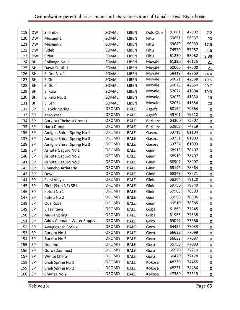
Groundwater potential assessment and characterization of Genale-Dawa River basin
Nebiyou k Page 65
119 DW Shambel SOMALI LIBEN Dolo Odo 816817
475029
7.2
120 DW Mesajid-1 SOMALI LIBEN Filtu 696512
569372
20
121 DW Mesajid-2 SOMALI LIBEN Filtu 696497
569396
17.5
122 DW Rideb SOMALI LIBEN Filtu 745700
579870
4.5
123 DW Sirba SOMALI LIBEN Filtu 612309
539822
2.86
124 BH Chilango No. 1 SOMALI LIBEN Moyale (SM)
613302
461257
21
125 BH Dawa South 1 SOMALI LIBEN Moyale (SM)
600000
475000
21
126 BH El Der No. 1 SOMALI LIBEN Moyale (SM)
584196
427695
24.4
127 BH El Gof SOMALI LIBEN Moyale (SM)
506212
425889
19.5
128 BH El Gof SOMALI LIBEN Moyale (SM)
506756
426502
20.7
129 BH El Kalu SOMALI LIBEN Moyale (SM)
520779
416940
19.3
130 BH El Kalu No. 1 SOMALI LIBEN Moyale (SM)
520357
416300
19
131 BH El Leh SOMALI LIBEN Moyale (SM)
520542
416545
20
132 SP Elabidu Spring OROMIYA
BALE Agarfa 601544
796640
0
133 SP Kasowara OROMIYA
BALE Agarfa 597012
796128
0
134 SP Burkitu (Cheketa Urene) OROMIYA
BALE Berbere 643000
753074
0
135 SP Haro Dumal OROMIYA
BALE Berbere 629588
747197
0
136 SP Amigna Shirar Spring No 1 OROMIYA
BALE Gasera 637197
811048
0
137 SP Amigna Shirar Spring No 2 OROMIYA
BALE Gasera 637319
810934
0
138 SP Amigna Shirar Spring No 3 OROMIYA
BALE Gasera 637345
810938
0
139 SP Ashute Gaguro No 1 OROMIYA
BALE Ginir 689134
784074
0
140 SP Ashute Gaguro No 2 OROMIYA
BALE Ginir 689107
784075
0
141 SP Ashute Gaguro No 3 OROMIYA
BALE Ginir 689075
784074
0
142 SP Chancho Ardaterie OROMIYA
BALE Ginir 691469
783643
0
143 SP Doyo OROMIYA
BALE Ginir 683496
785713
0
144 SP Elani Abiyu OROMIYA
BALE Ginir 682444
781206
0
145 SP Ginir (9km NE) SP1 OROMIYA
BALE Ginir 697500
797400
0
146 SP Keteti No 1 OROMIYA
BALE Ginir 699656
789934
0
147 SP Keteti No 2 OROMIYA
BALE Ginir 699580
789964
0
148 SP Oda Roba OROMIYA
BALE Ginir 695106
788858
0
149 SP Elasa Iteya OROMIYA
BALE Goba 618697
772454
0
150 SP Misira Spring OROMIYA
BALE Goba 619550
775382
0
151 SP Addis Alemana Water Supply Scheme
OROMIYA
BALE Goro 650476
776865
0
152 SP Awugiegesh Spring OROMIYA
BALE Goro 644261
770337
0
153 SP Burkitu No 1 OROMIYA
BALE Goro 666322
770991
0
154 SP Burkitu No 2 OROMIYA
BALE Goro 666325
770974
0
155 SP Dodimol OROMIYA
BALE Goro 657506
770936
0
156 SP Goro (Dadimos) OROMIYA
BALE Goro 665704
772100
0
157 SP Weltai Chefa OROMIYA
BALE Goro 664708
771782
0
158 SP Chali Spring No 1 OROMIYA
BALE Kokosa 482303
744555
0
159 SP Chali Spring No 2 OROMIYA
BALE Kokosa 482310
744566
0
160 SP Churisa No 2 OROMIYA
BALE Kokosa 473801
756158
0
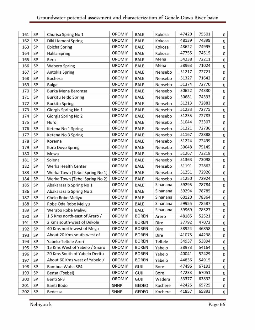
Groundwater potential assessment and characterization of Genale-Dawa River basin
Nebiyou k Page 66
161 SP Churisa Spring No 1 OROMIYA
BALE Kokosa 474209
755015
0
162 SP Diki Liemeni Spring OROMIYA
BALE Kokosa 481390
743991
0
163 SP Ebicha Spring OROMIYA
BALE Kokosa 486225
749952
0
164 SP Halila Spring OROMIYA
BALE Kokosa 477550
745157
0
165 SP Rera OROMIYA
BALE Mena Angetu
542381
722111
0
166 SP Wabero Spring OROMIYA
BALE Mena Angetu
589639
710249
0
167 SP Antokia Spring OROMIYA
BALE Nensebo 512176
727217
0
168 SP Bochesa OROMIYA
BALE Nensebo 513277
716429
0
169 SP Bulga OROMIYA
BALE Nensebo 513748
727700
0
170 SP Burka Mena Beromsa OROMIYA
BALE Nensebo 506224
743305
0
171 SP Burkitu Jeldo Spring OROMIYA
BALE Nensebo 506816
743339
0
172 SP Burkitu Spring OROMIYA
BALE Nensebo 512131
728839
0
173 SP Giorgis Spring No 1 OROMIYA
BALE Nensebo 512331
727751
0
174 SP Giorgis Spring No 2 OROMIYA
BALE Nensebo 512356
727837
0
175 SP Huro OROMIYA
BALE Nensebo 510447
733078
0
176 SP Ketena No 1 Spring OROMIYA
BALE Nensebo 512210
727368
0
177 SP Ketena No 3 Spring OROMIYA
BALE Nensebo 511676
728884
0
178 SP Korema OROMIYA
BALE Nensebo 512242
724995
0
179 SP Koro Doyo Spring OROMIYA
BALE Nensebo 506489
751450
0
180 SP Mewa OROMIYA
BALE Nensebo 512677
732181
0
181 SP Solena OROMIYA
BALE Nensebo 513637
730981
0
182 SP Werka Health Center OROMIYA
BALE Nensebo 511914
728625
0
183 SP Werka Town (Tebel Spring No 1) OROMIYA
BALE Nensebo 512517
729262
0
184 SP Werka Town (Tebel Spring No 2) OROMIYA
BALE Nensebo 512507
729245
0
185 SP Abakarazalo Spring No 1 OROMIYA
BALE Sinanana Dinsho
592952
787842
0
186 SP Abakarazalo Spring No 2 OROMIYA
BALE Sinanana Dinsho
592941
787853
0
187 SP Chelo Robe Meliyu OROMIYA
BALE Sinanana Dinsho
601204
783645
0
188 SP Robe Oda Robe Meliyu OROMIYA
BALE Sinanana Dinsho
599555
785878
0
189 SP Werabo Robe Meliyu OROMIYA
BALE Sinanana Dinsho
599691
785277
0
190 SP 1.5 Kms north-east of Arero / Metagefersa
OROMIYA
BORENA
Arero 481858
525216
0
191 SP 2 Kms south-west of Dekole spring (1) / Dokole (2)
OROMIYA
BORENA
Dire 377924
470726
0
192 SP 40 Kms north-west of Mega Dolola (1)
OROMIYA
BORENA
Dire 389246
468581
0
193 SP About 20 Kms south-west of Mega / Sake
OROMIYA
BORENA
Dire 410758
442388
0
194 SP Yabelo-Teltele Areri OROMIYA
BORENA
Teltele 349378
538949
0
195 SP 15 Kms West of Yabelo / Gnaro Village
OROMIYA
BORENA
Yabelo 389737
541642
0
196 SP 20 Kms South of Yabelo Deritu spring
OROMIYA
BORENA
Yabelo 400413
524294
0
197 SP About 60 Kms west of Yabelo / Sankura
OROMIYA
BORENA
Yabelo 448364
549154
0
198 SP Bambua Wuha SP4 OROMIYA
GUJI Bore 474961
671937
0
199 SP Bensa (Tsebel) OROMIYA
GUJI Bore 472335
670519
0
200 SP Benti SP3 OROMIYA
GUJI Wadera 533772
638325
0
201 SP Banti Bodo SNNP GEDEO Kochere 424257
657259
0
202 SP Bedessa SNNP GEDEO Kochere 418576
658935
0
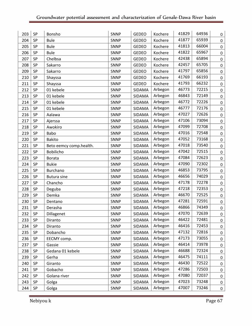
Groundwater potential assessment and characterization of Genale-Dawa River basin
Nebiyou k Page 67
203 SP Bonsho SNNP GEDEO Kochere 418290
649366
0
204 SP Bule SNNP GEDEO Kochere 418770
659399
0
205 SP Bule SNNP GEDEO Kochere 418137
660042
0
206 SP Bule SNNP GEDEO Kochere 418228
659675
0
207 SP Chelbsa SNNP GEDEO Kochere 424383
658949
0
208 SP Sakarro SNNP GEDEO Kochere 424579
657055
0
209 SP Sakarro SNNP GEDEO Kochere 417974
658563
0
210 SP Shayssa SNNP GEDEO Kochere 417699
661935
0
211 SP Shayssa SNNP GEDEO Kochere 417938
662324
0
212 SP 01 kebele SNNP SIDAMA Arbegona
467735
722158
0
213 SP 01 kebele SNNP SIDAMA Arbegona
468432
721493
0
214 SP 01 kebele SNNP SIDAMA Arbegona
467720
722265
0
215 SP 01 kebele SNNP SIDAMA Arbegona
467779
721767
0
216 SP Aalawa SNNP SIDAMA Arbegona
470275
726266
0
217 SP Ajerssa SNNP SIDAMA Arbegona
471064
730945
0
218 SP Awokiro SNNP SIDAMA Arbegona
470997
727085
0
219 SP Babo SNNP SIDAMA Arbegona
470165
725485
0
220 SP Bakito SNNP SIDAMA Arbegona
470528
731683
0
221 SP Beto eemcy comp.health. SNNP SIDAMA Arbegona
470188
735408
0
222 SP Bobilicho SNNP SIDAMA Arbegona
470420
725150
0
223 SP Borata SNNP SIDAMA Arbegona
470848
726233
0
224 SP Bukie SNNP SIDAMA Arbegona
470906
723025
0
225 SP Burchano SNNP SIDAMA Arbegona
468536
737959
0
226 SP Butura sine SNNP SIDAMA Arbegona
466567
740298
0
227 SP Chancho SNNP SIDAMA Arbegona
471780
722788
0
228 SP Deguba SNNP SIDAMA Arbegona
472189
723536
0
229 SP Demka SNNP SIDAMA Arbegona
466702
725259
0
230 SP Dentano SNNP SIDAMA Arbegona
472816
725914
0
231 SP Derasha SNNP SIDAMA Arbegona
468661
743494
0
232 SP Dillagenet SNNP SIDAMA Arbegona
470702
726393
0
233 SP Diranto SNNP SIDAMA Arbegona
464226
724814
0
234 SP Diranto SNNP SIDAMA Arbegona
464162
724532
0
235 SP Dobancho SNNP SIDAMA Arbegona
471322
728168
0
236 SP EECMY comp. SNNP SIDAMA Arbegona
471736
730551
0
237 SP Gassie SNNP SIDAMA Arbegona
464142
739784
0
238 SP Gedana 01 kebele SNNP SIDAMA Arbegona
466882
723240
0
239 SP Gerha SNNP SIDAMA Arbegona
464758
741115
0
240 SP Giranto SNNP SIDAMA Arbegona
464303
725223
0
241 SP Gobacho SNNP SIDAMA Arbegona
472865
725032
0
242 SP Golana river SNNP SIDAMA Arbegona
470800
720374
0
243 SP Golga SNNP SIDAMA Arbegona
470239
732481
0
244 SP Golga SNNP SIDAMA Arbegona
470073
732466
0
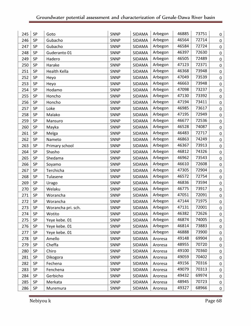
Groundwater potential assessment and characterization of Genale-Dawa River basin
Nebiyou k Page 68
245 SP Goto SNNP SIDAMA Arbegona
468853
737514
0
246 SP Gubacho SNNP SIDAMA Arbegona
465644
727141
0
247 SP Gubacho SNNP SIDAMA Arbegona
465844
727249
0
248 SP Guderanto 01 SNNP SIDAMA Arbegona
463974
726300
0
249 SP Hadero SNNP SIDAMA Arbegona
465059
724890
0
250 SP Harake SNNP SIDAMA Arbegona
471235
723711
0
251 SP Health Kella SNNP SIDAMA Arbegona
463685
739480
0
252 SP Heyo SNNP SIDAMA Arbegona
470494
735390
0
253 SP Heyo SNNP SIDAMA Arbegona
466630
739487
0
254 SP Hodamo SNNP SIDAMA Arbegona
470982
732378
0
255 SP Honcho SNNP SIDAMA Arbegona
471309
733923
0
256 SP Honcho SNNP SIDAMA Arbegona
471940
734119
0
257 SP Loke SNNP SIDAMA Arbegona
469859
736173
0
258 SP Malako SNNP SIDAMA Arbegona
471953
729497
0
259 SP Mansuro SNNP SIDAMA Arbegona
466775
725362
0
260 SP Mayka SNNP SIDAMA Arbegona
465287
740876
0
261 SP Melga SNNP SIDAMA Arbegona
464838
727175
0
262 SP Nameto SNNP SIDAMA Arbegona
468634
742495
0
263 SP Primary school SNNP SIDAMA Arbegona
463672
739137
0
264 SP Shasho SNNP SIDAMA Arbegona
468123
743267
0
265 SP Shedama SNNP SIDAMA Arbegona
469625
735431
0
266 SP Soyamo SNNP SIDAMA Arbegona
466107
726081
0
267 SP Terchicha SNNP SIDAMA Arbegona
473057
729044
0
268 SP Tulasene SNNP SIDAMA Arbegona
465723
727544
0
269 SP Urago SNNP SIDAMA Arbegona
468369
735944
0
270 SP Welaku SNNP SIDAMA Arbegona
467755
739170
0
271 SP Worancha SNNP SIDAMA Arbegona
470510
720918
0
272 SP Worancha SNNP SIDAMA Arbegona
471440
719751
0
273 SP Worancha pri. sch. SNNP SIDAMA Arbegona
471311
720018
0
274 SP Wotito SNNP SIDAMA Arbegona
463824
726262
0
275 SP Yeye kebe. 01 SNNP SIDAMA Arbegona
468748
740055
0
276 SP Yeye kebe. 01 SNNP SIDAMA Arbegona
468144
738835
0
277 SP Yeye kebe. 01 SNNP SIDAMA Arbegona
468885
739007
0
278 SP Amello SNNP SIDAMA Aroresa 491481
699041
0
279 SP Cheffa SNNP SIDAMA Aroresa 489555
707202
0
280 SP Chiro SNNP SIDAMA Aroresa 491007
703609
0
281 SP Dikogora SNNP SIDAMA Aroresa 490593
704023
0
282 SP Fechena SNNP SIDAMA Aroresa 491565
703166
0
283 SP Fenchena SNNP SIDAMA Aroresa 490794
703138
0
284 SP Gerbicho SNNP SIDAMA Aroresa 494320
699749
0
285 SP Merkata SNNP SIDAMA Aroresa 489454
707231
0
286 SP Muremura SNNP SIDAMA Aroresa 493277
689660
0
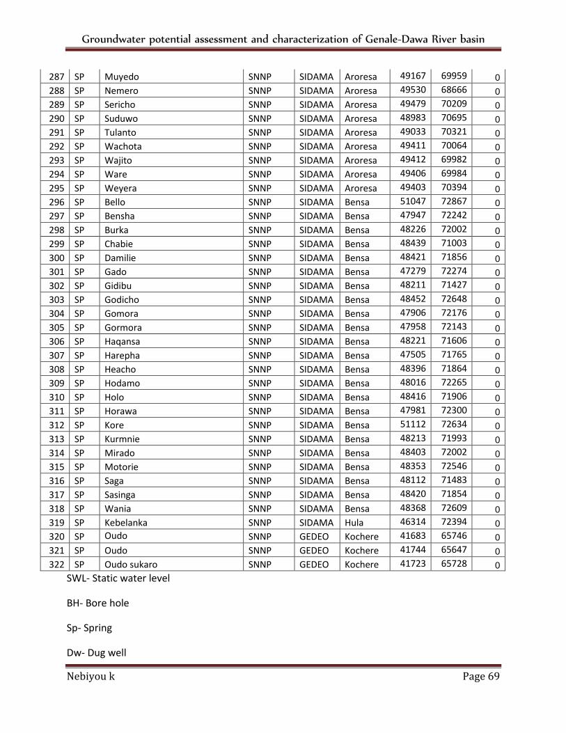
Groundwater potential assessment and characterization of Genale-Dawa River basin
Nebiyou k Page 69
287 SP Muyedo SNNP SIDAMA Aroresa 491672
699597
0
288 SP Nemero SNNP SIDAMA Aroresa 495300
686661
0
289 SP Sericho SNNP SIDAMA Aroresa 494792
702098
0
290 SP Suduwo SNNP SIDAMA Aroresa 489832
706958
0
291 SP Tulanto SNNP SIDAMA Aroresa 490332
703217
0
292 SP Wachota SNNP SIDAMA Aroresa 494118
700642
0
293 SP Wajito SNNP SIDAMA Aroresa 494128
699825
0
294 SP Ware SNNP SIDAMA Aroresa 494068
699848
0
295 SP Weyera SNNP SIDAMA Aroresa 494030
703943
0
296 SP Bello SNNP SIDAMA Bensa 510474
728674
0
297 SP Bensha SNNP SIDAMA Bensa 479475
722424
0
298 SP Burka SNNP SIDAMA Bensa 482263
720024
0
299 SP Chabie SNNP SIDAMA Bensa 484393
710030
0
300 SP Damilie SNNP SIDAMA Bensa 484218
718563
0
301 SP Gado SNNP SIDAMA Bensa 472792
722741
0
302 SP Gidibu SNNP SIDAMA Bensa 482117
714278
0
303 SP Godicho SNNP SIDAMA Bensa 484525
726487
0
304 SP Gomora SNNP SIDAMA Bensa 479066
721768
0
305 SP Gormora SNNP SIDAMA Bensa 479589
721436
0
306 SP Haqansa SNNP SIDAMA Bensa 482213
716069
0
307 SP Harepha SNNP SIDAMA Bensa 475059
717656
0
308 SP Heacho SNNP SIDAMA Bensa 483964
718640
0
309 SP Hodamo SNNP SIDAMA Bensa 480162
722654
0
310 SP Holo SNNP SIDAMA Bensa 484169
719061
0
311 SP Horawa SNNP SIDAMA Bensa 479815
723006
0
312 SP Kore SNNP SIDAMA Bensa 511126
726343
0
313 SP Kurmnie SNNP SIDAMA Bensa 482137
719930
0
314 SP Mirado SNNP SIDAMA Bensa 484038
720026
0
315 SP Motorie SNNP SIDAMA Bensa 483538
725464
0
316 SP Saga SNNP SIDAMA Bensa 481129
714834
0
317 SP Sasinga SNNP SIDAMA Bensa 484201
718546
0
318 SP Wania SNNP SIDAMA Bensa 483685
726092
0
319 SP Kebelanka SNNP SIDAMA Hula 463148
723949
0
320 SP Oudo SNNP GEDEO Kochere 416833
657460
0
321 SP Oudo SNNP GEDEO Kochere 417449
656471
0
322 SP Oudo sukaro SNNP GEDEO Kochere 417234
657283
0
SWL- Static water level
BH- Bore hole
Sp- Spring
Dw- Dug well
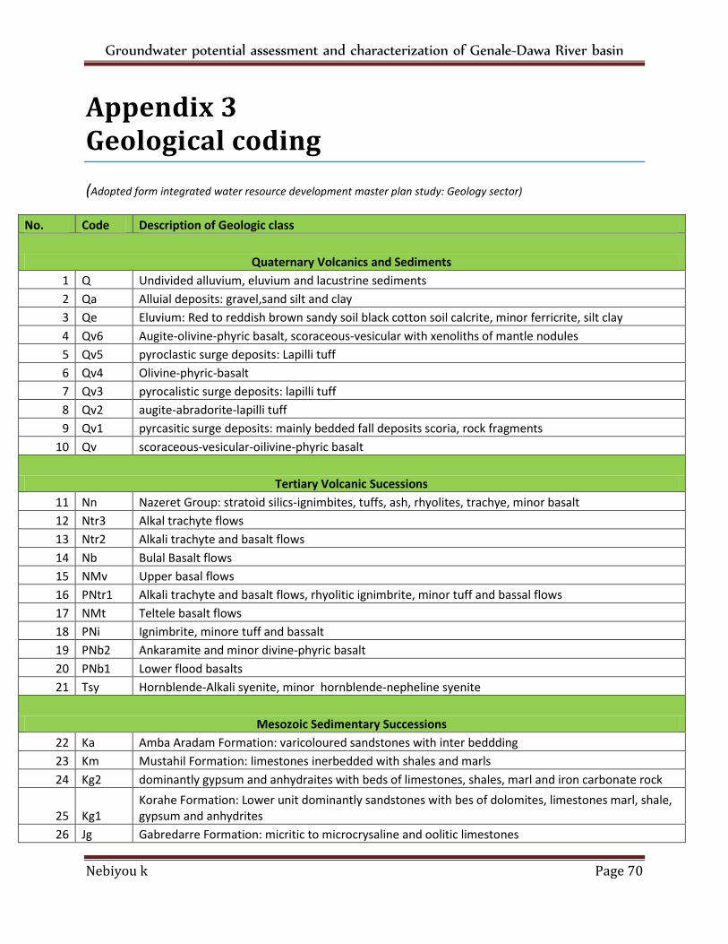
Groundwater potential assessment and characterization of Genale-Dawa River basin
Nebiyou k Page 70
Appendix 3 Geological coding
(Adopted form integrated water resource development master plan study: Geology sector)
No. Code Description of Geologic class
Quaternary Volcanics and Sediments
1 Q Undivided alluvium, eluvium and lacustrine sediments
2 Qa Alluial deposits: gravel,sand silt and clay
3 Qe Eluvium: Red to reddish brown sandy soil black cotton soil calcrite, minor ferricrite, silt clay
4 Qv6 Augite-olivine-phyric basalt, scoraceous-vesicular with xenoliths of mantle nodules
5 Qv5 pyroclastic surge deposits: Lapilli tuff
6 Qv4 Olivine-phyric-basalt
7 Qv3 pyrocalistic surge deposits: lapilli tuff
8 Qv2 augite-abradorite-lapilli tuff
9 Qv1 pyrcasitic surge deposits: mainly bedded fall deposits scoria, rock fragments
10 Qv scoraceous-vesicular-oilivine-phyric basalt
Tertiary Volcanic Sucessions
11 Nn Nazeret Group: stratoid silics-ignimbites, tuffs, ash, rhyolites, trachye, minor basalt
12 Ntr3 Alkal trachyte flows
13 Ntr2 Alkali trachyte and basalt flows
14 Nb Bulal Basalt flows
15 NMv Upper basal flows
16 PNtr1 Alkali trachyte and basalt flows, rhyolitic ignimbrite, minor tuff and bassal flows
17 NMt Teltele basalt flows
18 PNi Ignimbrite, minore tuff and bassalt
19 PNb2 Ankaramite and minor divine-phyric basalt
20 PNb1 Lower flood basalts
21 Tsy Hornblende-Alkali syenite, minor hornblende-nepheline syenite
Mesozoic Sedimentary Successions
22 Ka Amba Aradam Formation: varicoloured sandstones with inter beddding
23 Km Mustahil Formation: limestones inerbedded with shales and marls
24 Kg2 dominantly gypsum and anhydraites with beds of limestones, shales, marl and iron carbonate rock
25 Kg1 Korahe Formation: Lower unit dominantly sandstones with bes of dolomites, limestones marl, shale, gypsum and anhydrites
26 Jg Gabredarre Formation: micritic to microcrysaline and oolitic limestones
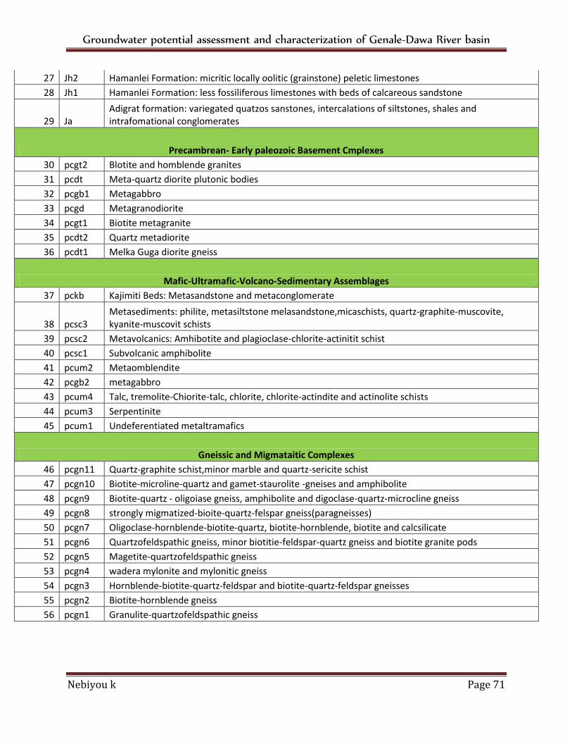
Groundwater potential assessment and characterization of Genale-Dawa River basin
Nebiyou k Page 71
27 Jh2 Hamanlei Formation: micritic locally oolitic (grainstone) peletic limestones
28 Jh1 Hamanlei Formation: less fossiliferous limestones with beds of calcareous sandstone
29 Ja Adigrat formation: variegated quatzos sanstones, intercalations of siltstones, shales and intrafomational conglomerates
Precambrean- Early paleozoic Basement Cmplexes
30 pcgt2 Blotite and homblende granites
31 pcdt Meta-quartz diorite plutonic bodies
32 pcgb1 Metagabbro
33 pcgd Metagranodiorite
34 pcgt1 Biotite metagranite
35 pcdt2 Quartz metadiorite
36 pcdt1 Melka Guga diorite gneiss
Mafic-Ultramafic-Volcano-Sedimentary Assemblages
37 pckb Kajimiti Beds: Metasandstone and metaconglomerate
38 pcsc3 Metasediments: philite, metasiltstone melasandstone,micaschists, quartz-graphite-muscovite, kyanite-muscovit schists
39 pcsc2 Metavolcanics: Amhibotite and plagioclase-chlorite-actinitit schist
40 pcsc1 Subvolcanic amphibolite
41 pcum2 Metaomblendite
42 pcgb2 metagabbro
43 pcum4 Talc, tremolite-Chiorite-talc, chlorite, chlorite-actindite and actinolite schists
44 pcum3 Serpentinite
45 pcum1 Undeferentiated metaltramafics
Gneissic and Migmataitic Complexes
46 pcgn11 Quartz-graphite schist,minor marble and quartz-sericite schist
47 pcgn10 Biotite-microline-quartz and gamet-staurolite -gneises and amphibolite
48 pcgn9 Biotite-quartz - oligoiase gneiss, amphibolite and digoclase-quartz-microcline gneiss
49 pcgn8 strongly migmatized-bioite-quartz-felspar gneiss(paragneisses)
50 pcgn7 Oligoclase-hornblende-biotite-quartz, biotite-hornblende, biotite and calcsilicate
51 pcgn6 Quartzofeldspathic gneiss, minor biotitie-feldspar-quartz gneiss and biotite granite pods
52 pcgn5 Magetite-quartzofeldspathic gneiss
53 pcgn4 wadera mylonite and mylonitic gneiss
54 pcgn3 Hornblende-biotite-quartz-feldspar and biotite-quartz-feldspar gneisses
55 pcgn2 Biotite-hornblende gneiss
56 pcgn1 Granulite-quartzofeldspathic gneiss
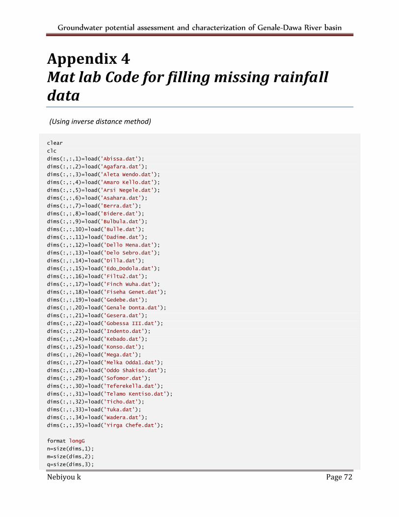
Groundwater potential assessment and characterization of Genale-Dawa River basin
Nebiyou k Page 72
Appendix 4 Mat lab Code for filling missing rainfall data
(Using inverse distance method)
clear
clc
dims(:,:,1)=load('Abissa.dat');
dims(:,:,2)=load('Agafara.dat');
dims(:,:,3)=load('Aleta Wendo.dat');
dims(:,:,4)=load('Amaro Kello.dat');
dims(:,:,5)=load('Arsi Negele.dat');
dims(:,:,6)=load('Asahara.dat');
dims(:,:,7)=load('Berra.dat');
dims(:,:,8)=load('Bidere.dat');
dims(:,:,9)=load('Bulbula.dat');
dims(:,:,10)=load('Bulle.dat');
dims(:,:,11)=load('Dadime.dat');
dims(:,:,12)=load('Dello Mena.dat');
dims(:,:,13)=load('Delo Sebro.dat');
dims(:,:,14)=load('Dilla.dat');
dims(:,:,15)=load('Edo_Dodola.dat');
dims(:,:,16)=load('Filtu2.dat');
dims(:,:,17)=load('Finch Wuha.dat');
dims(:,:,18)=load('Fiseha Genet.dat');
dims(:,:,19)=load('Gedebe.dat');
dims(:,:,20)=load('Genale Donta.dat');
dims(:,:,21)=load('Gesera.dat');
dims(:,:,22)=load('Gobessa III.dat');
dims(:,:,23)=load('Indento.dat');
dims(:,:,24)=load('Kebado.dat');
dims(:,:,25)=load('Konso.dat');
dims(:,:,26)=load('Mega.dat');
dims(:,:,27)=load('Melka Odda1.dat');
dims(:,:,28)=load('Oddo Shakiso.dat');
dims(:,:,29)=load('Sofomor.dat');
dims(:,:,30)=load('Teferekella.dat');
dims(:,:,31)=load('Telamo Kentiso.dat');
dims(:,:,32)=load('Ticho.dat');
dims(:,:,33)=load('Tuka.dat');
dims(:,:,34)=load('Wadera.dat');
dims(:,:,35)=load('Yirga Chefe.dat');
format longG
n=size(dims,1);
m=size(dims,2);
q=size(dims,3);
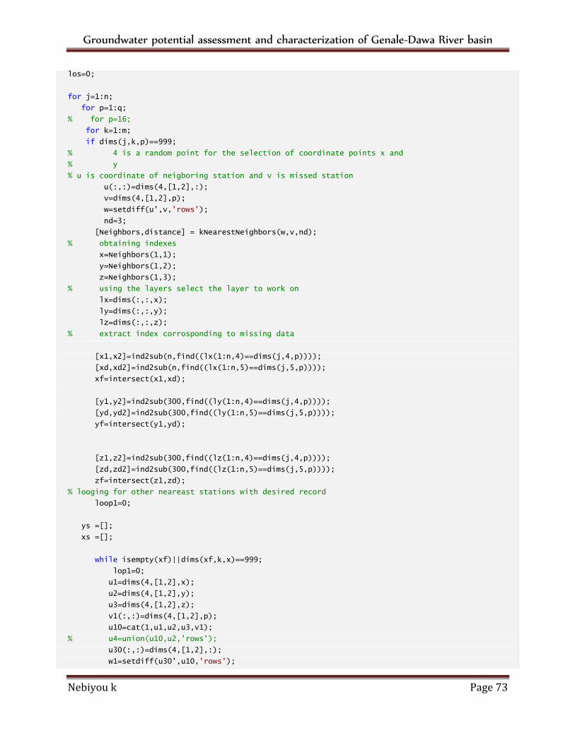
Groundwater potential assessment and characterization of Genale-Dawa River basin
Nebiyou k Page 73
los=0;
for j=1:n;
for p=1:q;
% for p=16;
for k=1:m;
if dims(j,k,p)==999;
% 4 is a random point for the selection of coordinate points x and
% y
% u is coordinate of neigboring station and v is missed station
u(:,:)=dims(4,[1,2],:);
v=dims(4,[1,2],p);
w=setdiff(u',v,'rows');
nd=3;
[Neighbors,distance] = kNearestNeighbors(w,v,nd);
% obtaining indexes
x=Neighbors(1,1);
y=Neighbors(1,2);
z=Neighbors(1,3);
% using the layers select the layer to work on
lx=dims(:,:,x);
ly=dims(:,:,y);
lz=dims(:,:,z);
% extract index corrosponding to missing data
[x1,x2]=ind2sub(n,find((lx(1:n,4)==dims(j,4,p))));
[xd,xd2]=ind2sub(n,find((lx(1:n,5)==dims(j,5,p))));
xf=intersect(x1,xd);
[y1,y2]=ind2sub(300,find((ly(1:n,4)==dims(j,4,p))));
[yd,yd2]=ind2sub(300,find((ly(1:n,5)==dims(j,5,p))));
yf=intersect(y1,yd);
[z1,z2]=ind2sub(300,find((lz(1:n,4)==dims(j,4,p))));
[zd,zd2]=ind2sub(300,find((lz(1:n,5)==dims(j,5,p))));
zf=intersect(z1,zd);
% looging for other neareast stations with desired record
loop1=0;
ys =[];
xs =[];
while isempty(xf)||dims(xf,k,x)==999;
lop1=0;
u1=dims(4,[1,2],x);
u2=dims(4,[1,2],y);
u3=dims(4,[1,2],z);
v1(:,:)=dims(4,[1,2],p);
u10=cat(1,u1,u2,u3,v1);
% u4=union(u10,u2,'rows');
u30(:,:)=dims(4,[1,2],:);
w1=setdiff(u30',u10,'rows');
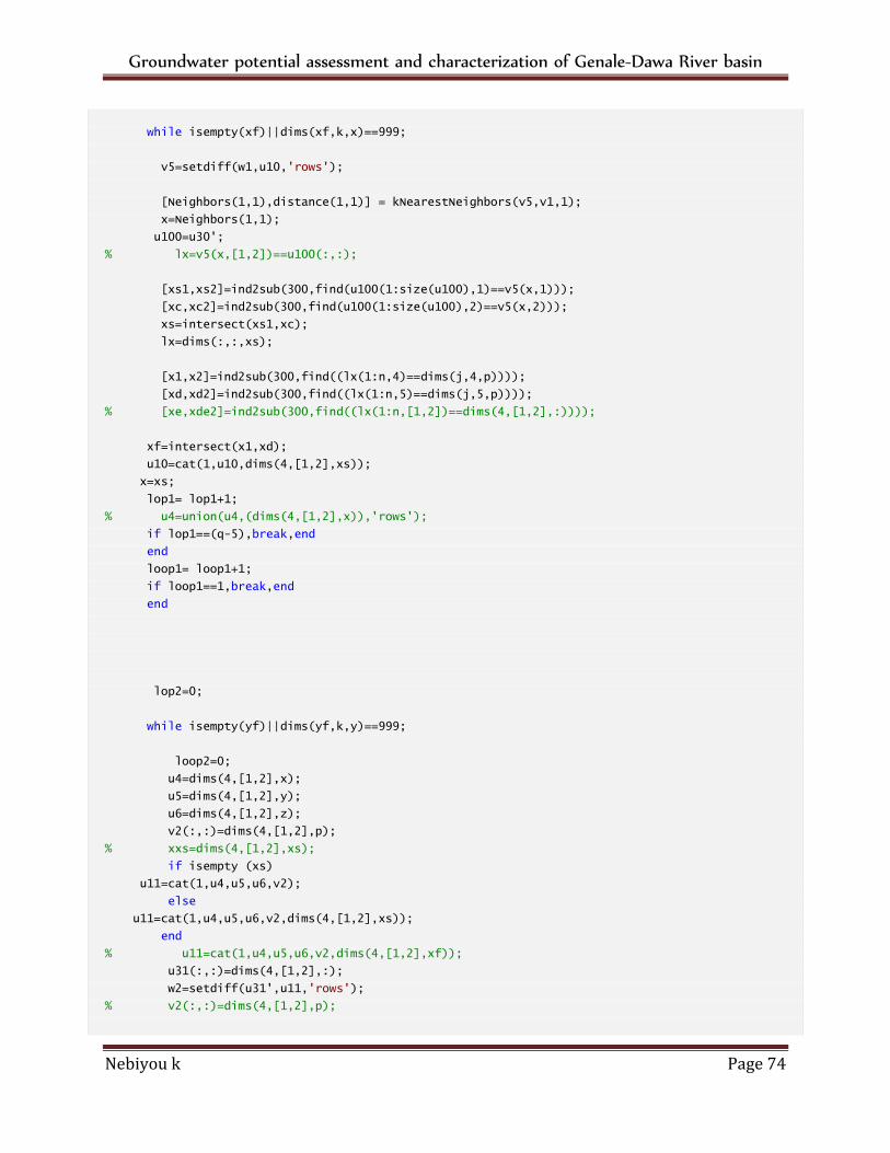
Groundwater potential assessment and characterization of Genale-Dawa River basin
Nebiyou k Page 74
while isempty(xf)||dims(xf,k,x)==999;
v5=setdiff(w1,u10,'rows');
[Neighbors(1,1),distance(1,1)] = kNearestNeighbors(v5,v1,1);
x=Neighbors(1,1);
u100=u30';
% lx=v5(x,[1,2])==u100(:,:);
[xs1,xs2]=ind2sub(300,find(u100(1:size(u100),1)==v5(x,1)));
[xc,xc2]=ind2sub(300,find(u100(1:size(u100),2)==v5(x,2)));
xs=intersect(xs1,xc);
lx=dims(:,:,xs);
[x1,x2]=ind2sub(300,find((lx(1:n,4)==dims(j,4,p))));
[xd,xd2]=ind2sub(300,find((lx(1:n,5)==dims(j,5,p))));
% [xe,xde2]=ind2sub(300,find((lx(1:n,[1,2])==dims(4,[1,2],:))));
xf=intersect(x1,xd);
u10=cat(1,u10,dims(4,[1,2],xs));
x=xs;
lop1= lop1+1;
% u4=union(u4,(dims(4,[1,2],x)),'rows');
if lop1==(q-5),break,end
end
loop1= loop1+1;
if loop1==1,break,end
end
lop2=0;
while isempty(yf)||dims(yf,k,y)==999;
loop2=0;
u4=dims(4,[1,2],x);
u5=dims(4,[1,2],y);
u6=dims(4,[1,2],z);
v2(:,:)=dims(4,[1,2],p);
% xxs=dims(4,[1,2],xs);
if isempty (xs)
u11=cat(1,u4,u5,u6,v2);
else
u11=cat(1,u4,u5,u6,v2,dims(4,[1,2],xs));
end
% u11=cat(1,u4,u5,u6,v2,dims(4,[1,2],xf));
u31(:,:)=dims(4,[1,2],:);
w2=setdiff(u31',u11,'rows');
% v2(:,:)=dims(4,[1,2],p);
Groundwater potential assessment and characterization of Genale-Dawa River basin
Nebiyou k Page 75
while isempty(yf)||dims(yf,k,y)==999;
v3=setdiff(w2,u11,'rows');
[Neighbors(1,2),distance(1,2)] = kNearestNeighbors(v3,v2,1);
Y=Neighbors(1,2);
% ly=dims(:,:,y);
u101=u31';
[Ys1,Ys2]=ind2sub(300,find(u101(1:size(u101),1)==v3(Y,1)));
[Yc,Yc2]=ind2sub(300,find(u101(1:size(u101),2)==v3(Y,2)));
ys=intersect(Ys1,Yc);
ly=dims(:,:,ys);
y=ys;
[y1,y2]=ind2sub(300,find((ly(1:n,4)==dims(j,4,p))));
[yd,yd2]=ind2sub(300,find((ly(1:n,5)==dims(j,5,p))));
yf=intersect(y1,yd);
loop2= loop2+1;
u11=cat(1,u11,(dims(4,[1,2],ys)));
if loop2==(q-5),break,end
end
lop2= lop2+1;
if lop2==1,break,end
end
lop3=0;
while isempty(zf)||dims(zf,k,z)==999;
loop3=0;
u7=dims(4,[1,2],x);
u8=dims(4,[1,2],y);
u9=dims(4,[1,2],z);
v4(:,:)=dims(4,[1,2],p);
if isempty(ys) && isempty (xs);
u12=cat(1,u7,u8,u9,v4);
elseif isempty (ys);
u12=cat(1,u7,u8,u9,v4,dims(4,[1,2],xs));
elseif isempty(xs);
u12=cat(1,u7,u8,u9,v4,dims(4,[1,2],ys));
elseif ~isempty(ys) && ~isempty (xs);
u12=cat(1,u7,u8,u9,v4,dims(4,[1,2],xs),dims(4,[1,2],ys));
end
% u12=cat(1,u7,u8,u9,v4,dims(4,[1,2],xf),dims(4,[1,2],yf));
% dims(4,[1,2],xs),dims(4,[1,2],Ys)
u32(:,:)=dims(4,[1,2],:);
Groundwater potential assessment and characterization of Genale-Dawa River basin
Nebiyou k Page 76
w3=setdiff(u32',u12,'rows');
% v7(:,:)=dims(4,[1,2],p);
while isempty(zf)||dims(zf,k,z)==999;
% u1(:,:)=dims(4,[1,2],:);
% w3=setdiff(u1',u2,'rows');
% v7(:,:)=dims(4,[1,2],p);
v7=setdiff(w3,u12,'rows');
[Neighbors(1,3),distance(1,3)] = kNearestNeighbors(v7,v4,1);
z=Neighbors(1,3);
u102=u32';
[zs1,zs2]=ind2sub(300,find(u102(1:size(u102),1)==v7(z,1)));
[zc,zc2]=ind2sub(300,find(u102(1:size(u102),2)==v7(z,2)));
zs=intersect(zs1,zc);
lz=dims(:,:,zs);
[z1,z2]=ind2sub(300,find((lz(1:n,4)==dims(j,4,p))));
[zd,zd2]=ind2sub(300,find((lz(1:n,5)==dims(j,5,p))));
zf=intersect(z1,zd);
u12=cat(1,u12,dims(4,[1,2],zs));
z=zs;
loop3= loop3+1;
% u12=union(u12,(dims(4,[1,2],zs)),'rows');
if loop3==(q-5),break,end
end
lop3= lop3+1;
if lop3==1,break,end
end
% Calculation by linear inverse distance for the respective conditions
if isempty(xf)&&(~isempty(zf)&&~isempty(yf));
if(((dims(zf,k,z)==999 || dims(yf,k,y)==999)));
if dims(zf,k,z)==999
dims(j,k,p)=dims(yf,k,y);
elseif dims(yf,k,y)==999
dims(j,k,p)=dims(zf,k,z);
end
elseif(((dims(zf,k,z)==999 && dims(yf,k,y)==999)));
dims(j,k,p)=999;
elseif(((dims(zf,k,z)~=999 && dims(yf,k,y)~=999)));
dims(j,k,p)=1/(1/distance(1,2)+1/distance(1,3))*((dims(zf,k,z)/distance(1,3)) +
(dims(yf,k,y)/distance(1,2)));
end
elseif isempty(yf)&&(~isempty(zf)&&~isempty(xf));
Groundwater potential assessment and characterization of Genale-Dawa River basin
Nebiyou k Page 77
if(((dims(xf,k,x)==999 || dims(zf,k,z)==999)));
if dims(xf,k,x)==999
dims(j,k,p)=dims(zf,k,z);
elseif dims(zf,k,z)==999
dims(j,k,p)=dims(xf,k,x);
end
elseif(((dims(xf,k,x)==999 && dims(zf,k,z)==999)))
dims(j,k,p)=999;
elseif(((dims(xf,k,x)~=999 && dims(zf,k,z)~=999)));
dims(j,k,p)=1/(1/distance(1,3)+1/distance(1,1))*((dims(xf,k,x)/distance(1,1)) +
(dims(zf,k,z)/distance(1,3)));
end
elseif isempty(zf)&&(~isempty(xf)&&~isempty(yf));
if(((dims(xf,k,x)==999 || dims(yf,k,y)==999)));
if dims(xf,k,x)==999
dims(j,k,p)=dims(yf,k,y);
elseif dims(yf,k,y)==999
dims(j,k,p)=dims(xf,k,x);
end
elseif(((dims(xf,k,x)==999 && dims(yf,k,y)==999)));
dims(j,k,p)=999;
elseif(((dims(xf,k,x)~=999 && dims(yf,k,y)~=999)));
dims(j,k,p)=1/(1/distance(1,2)+1/distance(1,1))*((dims(xf,k,x)/distance(1,1)) +
(dims(yf,k,y)/distance(1,2)));
end
elseif ((isempty(xf) && isempty(zf))&& isempty(yf));
dims(j,k,p)=999;
elseif ((isempty(xf) && isempty(zf))||(isempty(xf) &&
isempty(yf))||(isempty(zf) && isempty(yf)));
if(isempty(xf) && isempty(zf));
dims(j,k,p)=dims(yf,k,y);
elseif (isempty(xf) && isempty(yf));
dims(j,k,p)=dims(zf,k,z);
else
dims(j,k,p)=dims(xf,k,x);
end
else
if dims(zf,k,z)==999 && (dims(xf,k,x)~=999 &&
dims(yf,k,y)~=999)
dims(j,k,p)=1/(1/distance(1,1)+1/distance(1,2))*((dims(xf,k,x)/distance(1,1)) +
(dims(yf,k,y)/distance(1,2)));
elseif dims(xf,k,x)==999 && (dims(zf,k,z)~=999 &&
dims(yf,k,y)~=999)
dims(j,k,p)=1/(1/distance(1,2)+1/distance(1,3))*((dims(yf,k,y)/distance(1,2))+
(dims(zf,k,z)/distance(1,3)));
elseif dims(yf,k,y)==999 && (dims(zf,k,z)~=999 &&
dims(xf,k,x)~=999)
Groundwater potential assessment and characterization of Genale-Dawa River basin
Nebiyou k Page 78
dims(j,k,p)=1/(1/distance(1,1)+1/distance(1,3))*((dims(xf,k,x)/distance(1,1))
+(dims(zf,k,z)/distance(1,3)));
elseif (dims(zf,k,z)==999 &&
dims(xf,k,x)==999)||(dims(zf,k,z)==999 && dims(yf,k,y)==999)||(dims(yf,k,y)==999 &&
dims(xf,k,x)==999)
dims(j,k,p)=((dims(xf,k,x)+dims(yf,k,y)+dims(zf,k,z))-
(2*999));
elseif dims(zf,k,z)~=999 && (dims(xf,k,x)~=999 &&
dims(yf,k,y)~=999)
dims(j,k,p)=1/(1/distance(1,1)+1/distance(1,2)+1/distance(1,3))*((dims(xf,k,x)/distance(1,1))+(di
ms(yf,k,y)/distance(1,2)) +(dims(zf,k,z)/distance(1,3)));
else
dims(j,k,p)=1/(1/distance(1,1)+1/distance(1,2)+1/distance(1,3))*((dims(xf,k,x)/distance(1,1))+(di
ms(yf,k,y)/distance(1,2)) +(dims(zf,k,z)/distance(1,3)));
end
end
else
dims(j,k,p)= dims(j,k,p);
end
end
end
end
% los=los+1;
% if los==2,break,end
% end
% store the matrix in diffrent variables
Abissa=dims(:,:,1);
Agafara=dims(:,:,2);
AletaWendo=dims(:,:,3);
AmaroKello=dims(:,:,4);
ArsiNegele=dims(:,:,5);
Asahara=dims(:,:,6);
Berra=dims(:,:,7);
Bidere=dims(:,:,8);
Bulbula=dims(:,:,9);
Bulle=dims(:,:,10);
Dadime=dims(:,:,11);
DelloMena=dims(:,:,12);
DeloSebro=dims(:,:,13);
Dilla=dims(:,:,14);
Edo_Dodola=dims(:,:,15);
Filtu=dims(:,:,16);
FinchWuha=dims(:,:,17);
FisehaGenet=dims(:,:,18);
Gedebe=dims(:,:,19);
GenaleDonta=dims(:,:,20);
Groundwater potential assessment and characterization of Genale-Dawa River basin
Nebiyou k Page 79
Gesera=dims(:,:,21);
GobessaIII=dims(:,:,22);
Indento=dims(:,:,23);
Kebado=dims(:,:,24);
Konso=dims(:,:,25);
Mega=dims(:,:,26);
MelkaOdda=dims(:,:,27);
OddoShakiso=dims(:,:,28);
Sofomor=dims(:,:,29);
Teferekella=dims(:,:,30);
TelamoKentiso=dims(:,:,31);
Ticho=dims(:,:,32);
Tuka=dims(:,:,33);
Wadera=dims(:,:,34);
YirgaChefe=dims(:,:,35);
% save data in separate sheet
save Abissa1.dat Abissa -ascii
save Agafara1.dat Agafara -ascii
save AletaWendo1.dat AletaWendo -ascii
save AmaroKello1.dat AmaroKello -ascii
save ArsiNegele1.dat ArsiNegele -ascii
save Asahara1.dat Asahara -ascii
save Berra1.dat Berra -ascii
save Bidere1.dat Bidere -ascii
save Bulbula1.dat Bulbula -ascii
save Bulle1.dat Bulle -ascii
save Dadime1.dat Dadime -ascii
save DelloMena1.dat DelloMena -ascii
save DeloSebro1.dat DeloSebro -ascii
save Dilla1.dat Dilla -ascii
save Edo_Dodola1.dat Edo_Dodola -ascii
save Filtu1.dat Filtu -ascii
save FinchWuha1.dat FinchWuha -ascii
save FisehaGenet1.dat FisehaGenet -ascii
save Gedebe1.dat Gedebe -ascii
save GenaleDonta1.dat GenaleDonta -ascii
save Gesera1.dat Gesera -ascii
save GobessaIII1.dat GobessaIII -ascii
save Indento1.dat Indento -ascii
save Kebado1.dat Kebado -ascii
save Konso1.dat Konso -ascii
save Mega1.dat Mega -ascii
save MelkaOdda11.dat MelkaOdda -ascii
save OddoShakiso1.dat OddoShakiso -ascii
save Sofomor1.dat Sofomor -ascii
save Teferekella1.dat Teferekella -ascii
save TelamoKentiso1.dat TelamoKentiso -ascii
save Ticho1.dat Ticho -ascii
save Tuka1.dat Tuka -ascii
save Wadera1.dat Wadera -ascii
save YirgaChefe1.dat YirgaChefe -ascii

Groundwater potential assessment and characterization of Genale-Dawa River basin
Nebiyou k Page 80
Related Documents


![Groundwater Investigation and Characterization · Groundwater Investigation and Characterization ... manual for environmental site characterization [2] ... through drilling, well](https://static.cupdf.com/doc/110x72/5b4001557f8b9a5e528ccc77/groundwater-investigation-and-characterization-groundwater-investigation-and.jpg)


