Ground water Fourth Years 1 Ground water Porous media characteristics Flow in porous media (Darcy eq.) Aquifer system General flow equation and its solution Advection dispersion relations Control methods of some ground water pollution situation

Welcome message from author
This document is posted to help you gain knowledge. Please leave a comment to let me know what you think about it! Share it to your friends and learn new things together.
Transcript
Ground water Fourth Years
1
Ground water
Porous media characteristics
Flow in porous media (Darcy eq.)
Aquifer system
General flow equation and its solution
Advection dispersion relations
Control methods of some ground water pollution situation
Ground water Fourth Years
2
Groundwater: is water stored under the surface of the ground in the tiny pore spaces between
rock, sand, soil, and gravel. It occurs in two “zones”: an upper, unsaturated zone where most of
the pore spaces are filled with air, and a deeper, saturated zone in which all the pore spaces are
filled with water
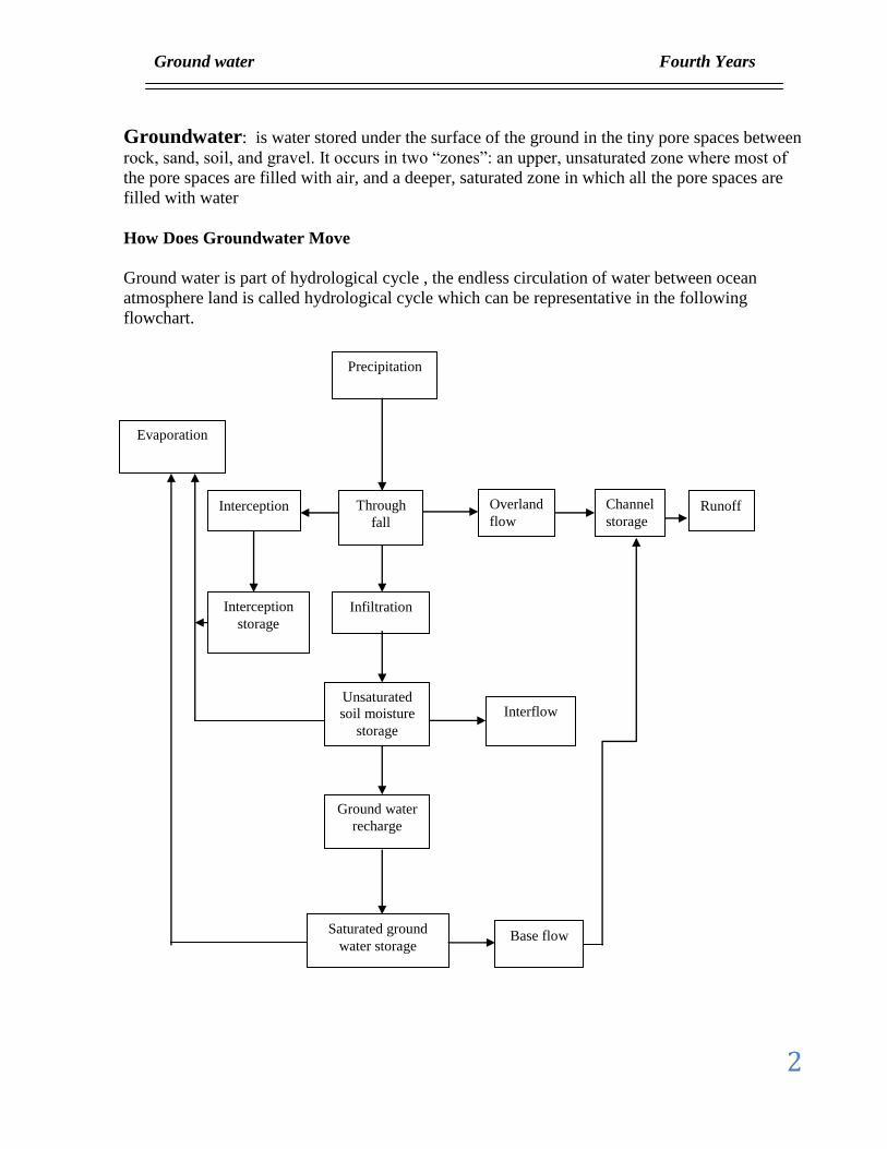
How Does Groundwater Move
Ground water is part of hydrological cycle , the endless circulation of water between ocean
atmosphere land is called hydrological cycle which can be representative in the following
flowchart.
Precipitation
Through
fall
Overland
flow
Channel
storage Runoff
Infiltration
Interception
Unsaturated
soil moisture
storage
Ground water
recharge
Saturated ground
water storage
Interflow
Base flow
Evaporation
Interception
storage
Ground water Fourth Years
3
Ground water is more than a resource , it is an important feature of the natural environmental
because , it leads to:
1. environmental problems through ground water contamination by:
Waste disposal technique (sanitary landfill for solid waste and deep well injection for
liquid waste).
Subsurface pollution can be caused by leakage from ponds and lagoons (which are
widely used as components of larger waste – disposal systems).
Leaching of animal waste , fertilizers and pesticide from agricultural soils.
2. Ground water contributors to geotechnical problems as slope stability and land
subsidence through withdrawals from subsurface aquifers
3. Ground water is a key to understanding a wide variety of earthquakes, the migration and
accumulation of petroleum.
The most geologic role played by ground water lies in the control that fluid pressures
exert on the mechanisms of faulting and thrusting.
All rocks that underline the earth’s surface can be classified either as aquifers or as
confined beds.
Aquifer: is a rock unit that will yield water in a usable quantity to a well or spring or a
permeable water bearing bed or layer that hold and transmit water.
Confined bed : is a rock unit having very low hydraulic conductivity that restricts the
movement of ground water either into or out of adjacent aquifers.
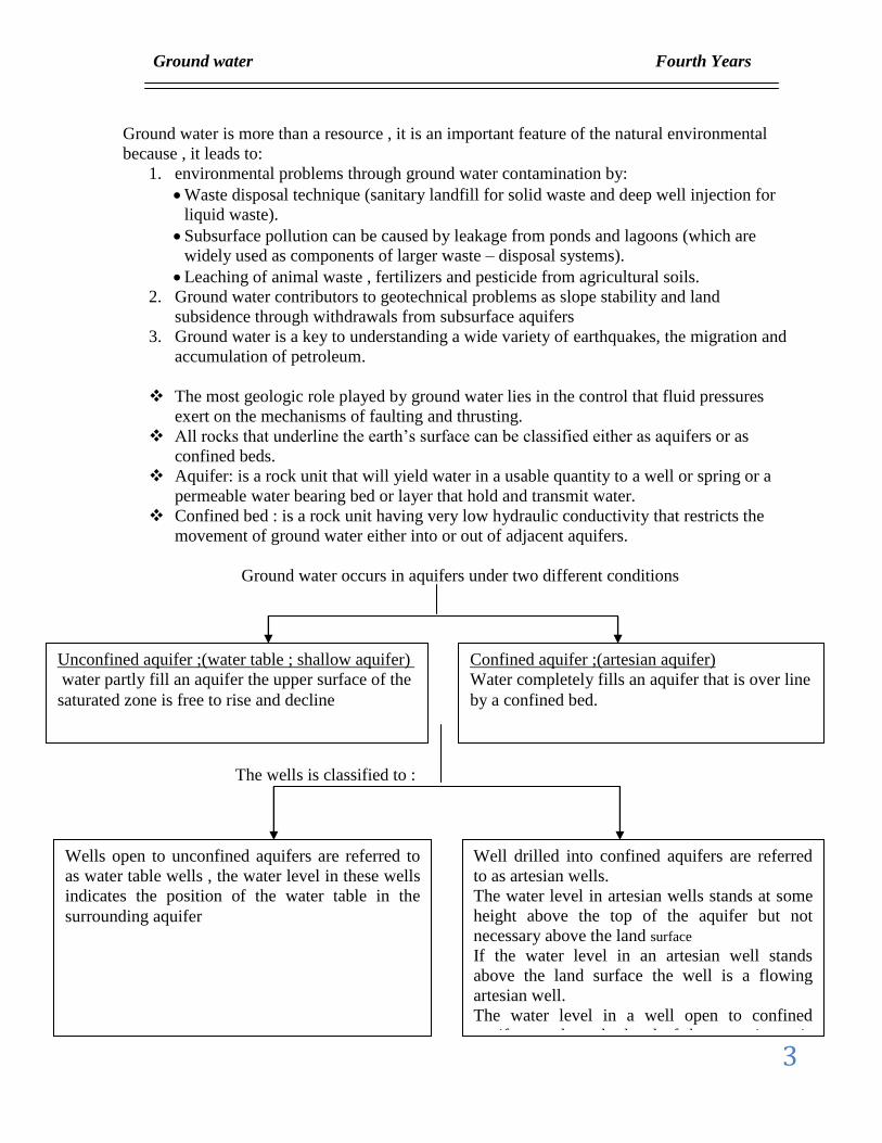
Ground water occurs in aquifers under two different conditions
The wells is classified to :
Unconfined aquifer ;(water table ; shallow aquifer)
water partly fill an aquifer the upper surface of the
saturated zone is free to rise and decline
fer);(artesian aqui Confined aquifer
Water completely fills an aquifer that is over line
by a confined bed.
Wells open to unconfined aquifers are referred to
as water table wells , the water level in these wells
indicates the position of the water table in the
surrounding aquifer
Well drilled into confined aquifers are referred
to as artesian wells.
The water level in artesian wells stands at some
height above the top of the aquifer but not
necessary above the land surface
If the water level in an artesian well stands
above the land surface the well is a flowing
artesian well.
The water level in a well open to confined
aquifer stands at the level of the potentiometric
surface of the aquifer
Ground water Fourth Years
4
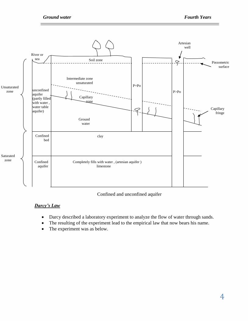
Confined and unconfined aquifer
Darcy’s Law
Darcy described a laboratory experiment to analyze the flow of water through sands.
The resulting of the experiment lead to the empirical law that now bears his name.
The experiment was as below.
Saturated
zone
Unsaturated
zone
Completely fills with water , (artesian aquifer )
limestone
clay
Ground
water
Confined
aquifer
Confined
bed
unconfined
aquifer
(partly filled
with water ,
water table
aquifer)
Capillary
zone
Capillary
fringe
Intermediate zone
unsaturated
Soil zone
Artesian
well
Piezometric
surface
P=Po
P>Po
River or
sea

Ground water Fourth Years
5
A circular cylinder of cross section A is filled with sand stoppered at each end and out
filled within flow and outflow tubes and a pair of manometers.
Water is introduced into the cylinder and allowed to flow through it until such time as all
the pores are filled with water and as get .
Qin = Qout
Set an arbitrary datum at elevation Z=0
The elevation of the manometers intakes are Z1 and Z2 , and
The elevation of fluid levels are h1 and h2
∆L = distance between manometer intakes
The specific discharge through the cylinder (v) is defined as:
A
Qv (has dimension of velocity)
Darcy velocity , flux velocity
The experiments carried out by Darcy showed that
Q
Q
Datum z=0
Z2 Z1
h2 h1
∆h
Cross sectional
area (A) ∆L
Ground water Fourth Years
6
Lv
hhv
1
21
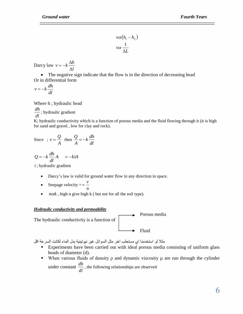
Darcy law l
hkv
The negative sign indicate that the flow is in the direction of decreasing head
Or in differential form
dl
dhkv
Where h ; hydraulic head
dl
dh; hydraulic gradient
K; hydraulic conductivity which is a function of porous media and the fluid flowing through it (it is high
for sand and gravel , low for clay and rock).
Since ; A
Qv then
dl
dhk
A
Q
kiAAdl
dhkQ
i ; hydraulic gradient
Darcy’s law is valid for ground water flow in any direction in space.
Seepage velocity =n
v
kn , high n give high k ( but not for all the soil type).
Hydraulic conductivity and permeability
Porous media
The hydraulic conductivity is a function of
Fluid
مثال لو استخدمنا اي مستحلب اخر مثل السوائل غير نيوتينية بدل الماء لكانت السرعة اقل
Experiments have been carried out with ideal porous media consisting of uniform glass
beads of diameter (d).
When various fluids of density ρ and dynamic viscosity µ are run through the cylinder
under constant dl
dh, the following relationships are observed

Ground water Fourth Years
7
1
2
v
gv
dv
Combining the above relation with Darcy law then
dl
dhgcdv
2
………………(1)
Where ; c= constant of proportionality (dimensionless constant)(depends on media properties ) such as :
1. Distribution of grain sizes
2. The sphericity and roundness of the grain
3. The nature of packing
Comparison with the original Darcy equation shows
gcdK
2
Where; ρ and µ are function of fluid alone 2cd are function of medium alone
If we define 2cdk then
gkK
Where k is a function of the medium and has dimensions (L2)
Hydraulic head and fluid potential
The word potential refer to the transport due to gradient (from high to law)
The fluid potential θ is to determined the potential gradient that controls the flow of water
through porous media.
Two obvious possibilities for potential quantity ; elevation and fluid pressure
For Darcy experiment , flow occur down through the cylinder (from high to low
elevation).
If θ=90 (cylinder were placed in a horizontal position),gravity play no role.
If θ=0 (vertical cylinder), flow would occur down through the cylinder from high
elevation to low in response to gravity.
Flow induced by increasing the pressure at one end and decreasing it at the
other
That is lead to energy loss
The classical definition of potential is the work done during the flow process.
Ground water Fourth Years
8
The work done in moving a unit mass of fluid between any two points in a flow system is
a measure of the energy loss of a unit mass.
Fluid through porous media is a mechanical process , the forces driving the fluid forward
most overcome the frictional forces set up between the moving fluid and grains of the
porous media.
The flow is therefore accompanied by an irreversible transformation of mechanical
energy to thermal energy through the mechanism of friction resistance.
Friction direction from high mechanical energy /unit mass lower
Mechanical energy defined as work required to move a unit mass from point to point.
Therefore ; fluid potential θ for low in porous media is the mechanical energy per unit
mass of fluid.
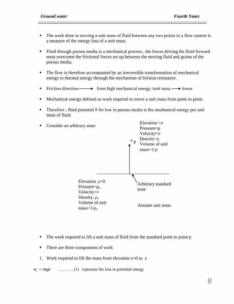
Consider an arbitrary state:
* p
The work required to lift a unit mass of fluid from the standard point to point p
There are three components of work
1. Work required to lift the mass from elevation z=0 to z
mgzw 1 …………(1) represent the loss in potential energy
Elevation =z
Pressure=p
Velocity=v
Dencity=ρ
Volume of unit
mass=1/ρ
Elevation ,z=0
Pressure=po
Velocity=v
Density, ρo
Volume of unit
mass=1/ρo
Arbitrary standard
state
Assume unit mass
Ground water Fourth Years
9
2. Work required to accelerate the fluid from velocity v=0 to v
2
2
2
mvw ……..(2) represent loss due to kinetic energy
3. Work done on the fluid in raising the fluid pressure from po to p
p
p
p
po o
dpmdp
m
vmw
3 …………(3) represent loss due to elastic energy
اخذنا تكامل الن الضغط هو قوة على وحدة مساحة المساحة هي تكامل
The fluid potential θ (mechanical energy / unit mass) is the sum of 321 www
p
po
dpm
mvmgz
2
2
for m=1
p
po
dpvgz
2
2
(Bernoulli equation)
For porous media (v) are low , so the second term will ignored.
For incompressible fluid ( fluid will constant density so that ρ is not a function of p)
opp
gz
………….(4)
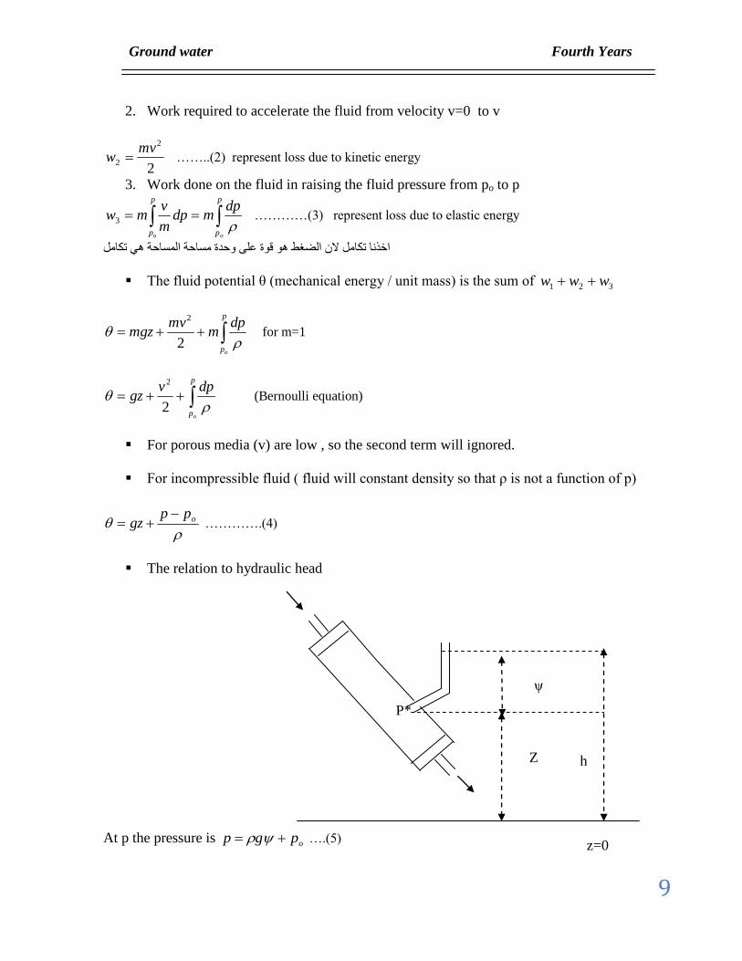
The relation to hydraulic head
At p the pressure is opgp ….(5)
z=0
Z h
ψ
P*

Ground water Fourth Years
10
zh
Elevation head pressure head
= height of the liquid column above p
op = atmospheric pressure
opzhgp …..(6) sub. (6) in (4)
oo ppzhg
gz
Then ghzhggz ……(7)
Where: g is constant of the earth surface
Θ :units of energy / unit mass
h: units of energy / unit mass
In ground water hydrology 0op and work in gage pressure (pressure above atmospheric
pressure), therefore equation (6) will be
zhgp ……..(8) sub. In (4)
ghzhg
gzp
gz
)( …..(9)
pgzgh dividing by g
g
pzh
.(10)
The term of gage pressure yields
gp ……(11) sub. In (10)
g
gzh
If we put Bernoulli equation in term of head
vpzt hhhh
Where : total head= elevation head + pressure head+ velocity head
Ground water moves in the direction of decreasing total head may or may not be in the
direction of decreasing pressure head.
Ground water Fourth Years
11
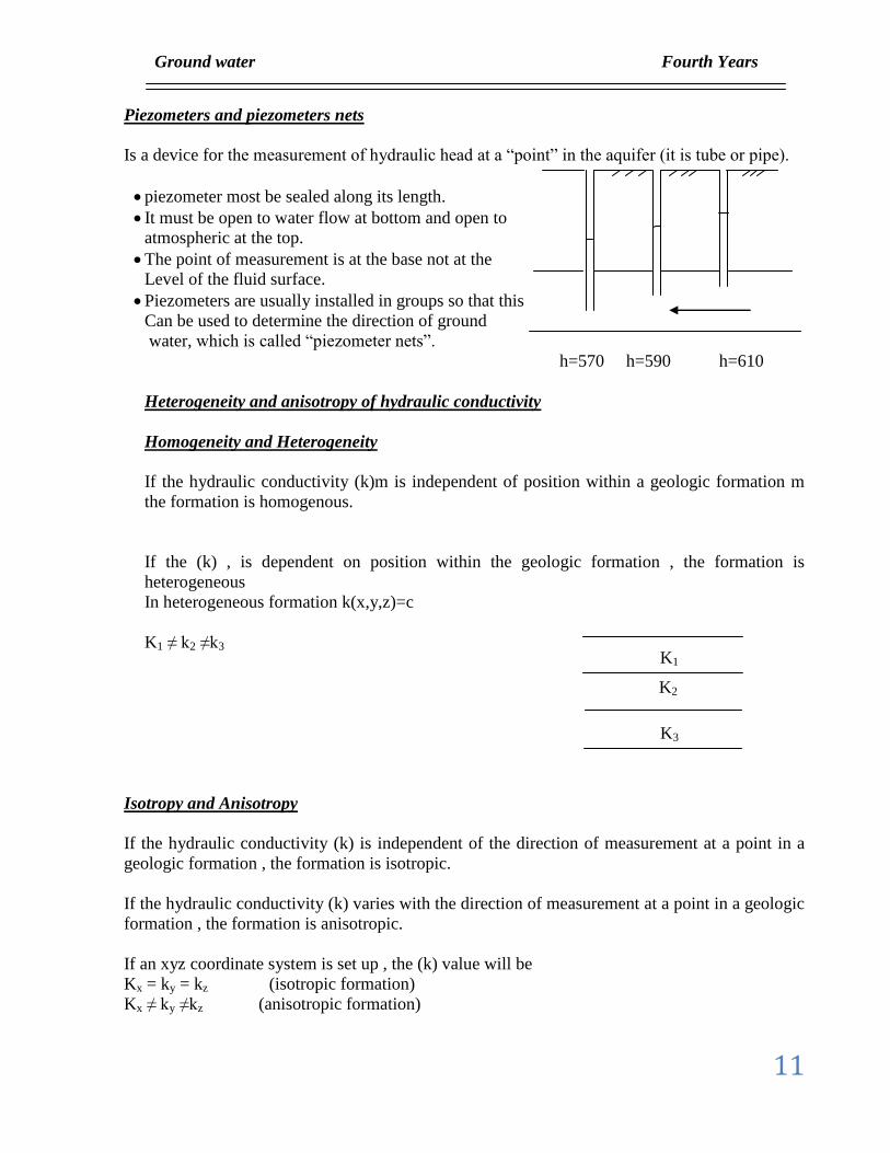
Piezometers and piezometers nets
Is a device for the measurement of hydraulic head at a “point” in the aquifer (it is tube or pipe).
piezometer most be sealed along its length.
It must be open to water flow at bottom and open to
atmospheric at the top.
The point of measurement is at the base not at the
Level of the fluid surface.
Piezometers are usually installed in groups so that this
Can be used to determine the direction of ground
water, which is called “piezometer nets”.
h=570 h=590 h=610
Heterogeneity and anisotropy of hydraulic conductivity
Homogeneity and Heterogeneity
If the hydraulic conductivity (k)m is independent of position within a geologic formation m
the formation is homogenous.
If the (k) , is dependent on position within the geologic formation , the formation is
heterogeneous
In heterogeneous formation k(x,y,z)=c
K1 ≠ k2 ≠k3
Isotropy and Anisotropy
If the hydraulic conductivity (k) is independent of the direction of measurement at a point in a
geologic formation , the formation is isotropic.
If the hydraulic conductivity (k) varies with the direction of measurement at a point in a geologic
formation , the formation is anisotropic.
If an xyz coordinate system is set up , the (k) value will be
Kx = ky = kz (isotropic formation)
Kx ≠ ky ≠kz (anisotropic formation)
K1
K2
K3
Ground water Fourth Years
12
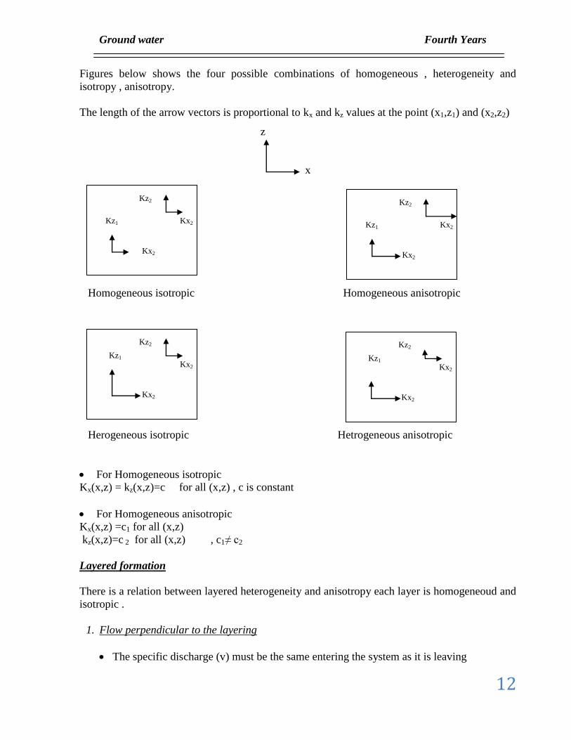
Figures below shows the four possible combinations of homogeneous , heterogeneity and
isotropy , anisotropy.
The length of the arrow vectors is proportional to kx and kz values at the point (x1,z1) and (x2,z2)
Homogeneous isotropic Homogeneous anisotropic
Herogeneous isotropic Hetrogeneous anisotropic
For Homogeneous isotropic
Kx(x,z) = kz(x,z)=c for all (x,z) , c is constant
For Homogeneous anisotropic
Kx(x,z) =c1 for all (x,z)
kz(x,z)=c 2 for all (x,z) , c1≠ c2
Layered formation
There is a relation between layered heterogeneity and anisotropy each layer is homogeneoud and
isotropic .
1. Flow perpendicular to the layering
The specific discharge (v) must be the same entering the system as it is leaving
z
x
Kz2
Kx2 Kz1
Kx2
Kz2
Kx2 Kz1
Kx2
Kz2
Kx2 Kz1
Kx2
Kz2
Kx2 Kz1
Kx2
Ground water Fourth Years
13
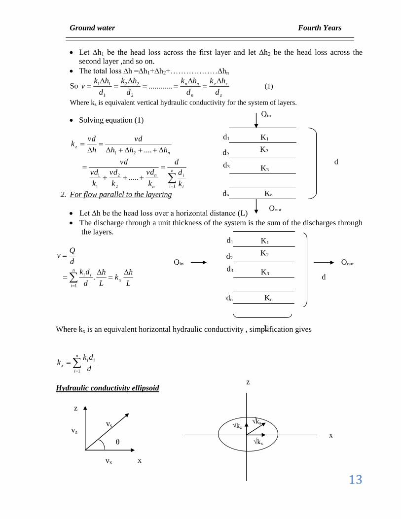
Let ∆h1 be the head loss across the first layer and let ∆h2 be the head loss across the
second layer ,and so on.
The total loss ∆h =∆h1+∆h2+………………∆hn
So z
zz
n
nn
d
hk
d
hk
d
hk
d
hkv
............
2
22
1
11 (1)
Where kz is equivalent vertical hydraulic conductivity for the system of layers.
Solving equation (1)
n
i i
i
n
n
n
z
k
d
d
k
vd
k
vd
k
vd
vd
hhh
vd
h
vdk
12
2
1
1
21
.....
....
2. For flow parallel to the layering
Let ∆h be the head loss over a horizontal distance (L)
The discharge through a unit thickness of the system is the sum of the discharges through
the layers.
n
i
x
ii
L
hk
L
h
d
dk
d
Qv
1
.
Where kx is an equivalent horizontal hydraulic conductivity , simplification gives
n
i
ii
xd
dkk
1
Hydraulic conductivity ellipsoid
K1
K2
K3
Kn
d1
d2
d3
dn
d
Qin Qout
L
K1
K2
K3
Kn
d1
d2
d3
dn
d
Qin
Qout
z
vs vz
x
θ
vx
z
x
√kz
√kx
√ks
Ground water Fourth Years
14
Consider an arbitrary flow line in the xz plane in a homogeneous anisotropic medium with kx and
kz .
The flow line
s
hkv s
(1)
Where ks is the unknown and it lies in range kx __kz
vs can be separate into its components vx and vz where
sin.
cos.
szz
sxx
vz
hkv
vx
hkv
(2)
Since h=h(x,z)
s
z
z
h
s
x
x
h
s
h
.. (3)
Geometrically , cos
s
x and sin
s
z
Substituting in equation (3) and combine with (1) and (2) yields
zxs
z
s
x
s
s
s
kkk
k
v
k
v
k
v
22 sincos1
sin.sin
cos.cos.
In angular direction by setting cosrx and sinrz we get
zxs k
z
k
x
k
r 222
Darcy’s law in three dimensions
In the dimensional flow , v is a vector with components zyx vvv ,,
z
hkv
y
hkv
x
hkv
zz
yy
xx
Ground water Fourth Years
15
Since (h) is a function of x , y ,z the derivative must be partial , so the more generalized set of
equations could be written in the form.
z
hk
y
hk
x
hkv
z
hk
y
hk
x
hkv
z
hk
y
hk
x
hkv
zzzyxzz
yzyyyxy
xzxyxxx
If we put components of k in matrix form , it is known as the hydraulic conductivity tenser.
zzzyzx
yzyyyx
xzxyxx
kkk
kkk
kkk
For general case 0 zyzxyzyxxzxy kkkkkk
Limitation of Darcy’s equation
1. Laminar flow 0.1≤Re≤10
2. Homogeneous and isotropic flow zyx kkk
3. No capillary zone
4. Steady state flow 0dt
dv
5. Hydraulic head is the only driving force 6. Incompressible fluid (ρ constant) 7. Full saturated zone.
Un saturated flow
Darcy’s law and the concepts of hydraulic head and hydraulic conductivity have been developed
for saturated porous media and it is clear that some soils are partially filled with water and the
other pores are filled with air . The flow of water under such conditions is called unsaturated or
partially saturated flow.
Moisture content
If the total unit volume Tv of a soil or rock is divided into the volume of the solid portion sv , the
volume of the water wv and the volume of air av the volumetric moisture content θ is defined as
T
w
v
v like porosity , n
n for saturated
n for unsaturated
Ground water Fourth Years
16
Water table
Is defined as the boundary between saturated and unsaturated zone and the fluid pressure (p) of it
in the pores of a porous medium is exactly atmospheric , po= 0 ( in gage pressure) ψ=0
Since zh , the hydraulic head at any point on water table must be equal to the elevation z of the
water table at that point.
Negative pressure head
So we have 0 in the saturated zone
0 in water table
0 in the unsaturated zone
This reflects the fact that water in the unsaturated zone is held in the soil pores under surface tension
forces.
Regardless of the sign ψ , the hydraulic head (h) is still equal z
However , above the water table , when 0 , piezometers are no longer a suitable instrument for
measurement of h, so head (h) must be obtained indirectly from measurement of determined with
tensiometers.
النه يحصل هناك تحدب بين الدقائق بسبب وجود الهواء والماء بسبب الخاصية الشعرية والشد السطحي التي تؤثر على الضغط
وتؤدي الى ان يكون الضغط اقل من الصفرز
Saturated , unsaturated zone
For saturated zone
1. It occurs below the water table.
2. The soil pores are filled with water and n
3. The fluid pressure P is greater than atmospheric so the pressure head (measured as gage pressure)
is greater than zero.
4. The hydraulic head must be measured with a piezometers.
5. The hydraulic conductivity k is a constant , it is not a function of pressure head
For unsaturated zone
1. It occurs above the water table and above the capillary fringes.
2. The soil pores are only partially filled with water, the moisture content θ is less than the porosity.
3. The fluid pressure id less than the atmospheric, the pressure head is less than zero.
4. The hydraulic head must be measured with a tensiometer.
5. The hydraulic conductivity and the moisture content are both function of the pressure head.
Transmissivity and stortivity
There are six basic properties of fluid and porous media that must be known in order to describe the
hydraulic aspect of saturated ground water flow
Ground water Fourth Years
17
For water
Density,
Viscosity,
Compressibility ,
For media
Porosity n (or void ratio , e)
Permeability , k
Compressibility ,
All the other parameters that are used to describe the hydro geologic propertied of geologic formations
can be derived from these six properties.
Specific storage , Ss
Ss , of a saturated aquifer is the volume of water that a unit volume of water that a unit volume of aquifer
releases from storage under a unit decline in hydraulic head (L-1
).
ngSs
Where = aquifer compressibility (media)
=water compressibility
Ss, the volume/ unit volume / unit of decline in head
For a confined aquifer
Transmissivity or transmissibility (T) is define as
kbT
Where b = aquifer thickness
Storitivity or storage coefficient (S) is define as
bSsS .
The stortivity of a saturated confined aquifer of thickness (b) is the volume of water that an aquifer
releases from storage per unit surface area of aquifer per unit decline in the component of hydraulic head
normal to the surface.
bngS .
It is possible to define a parameter that couples the transmissivity properties T or k and the storage
properties S , Ss which is the hydraulic diffusivity D
Ss
k
bSs
bk
S
TD
.
.
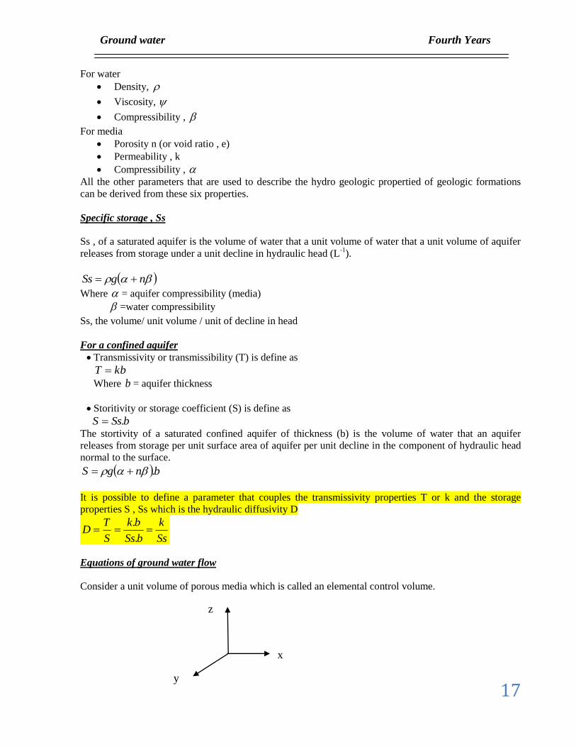
Equations of ground water flow
Consider a unit volume of porous media which is called an elemental control volume.
z
y
x
Ground water Fourth Years
18
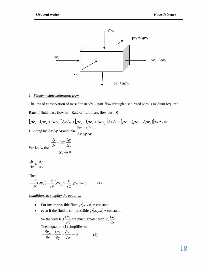
1. Steady – state saturation flow
The law of conservation of mass for steady – state flow through a saturated porous medium required.
Rate of fluid mass flow in = Rate of fluid mass flow out = 0
yxvvvzxvvvzyvvv zzzyyyxxx ...
Dividing by zyx .. and take zyx
..
0lim
We know that
0
lim
x
x
y
dx
dy
x
y
dx
dy
Then
0
zyx v
zv
yv
x (1)
Conditions to simplify the equation
For incompressible fluid zyx .. constant
even if the fluid is compressible zyx .. constant.
So the term bx
vx
are much greater than
xvx
Then equation (1) simplifies to
0
z
v
y
v
x
v zyx (2)
vzρ
vxρ
vyρ
vz +∆ρvzρ
vx+∆ρvxρ
vy +∆ρvyρ
Ground water Fourth Years
19
Substitution of Darcy’s law for zyx vvv ,, equation (2) yields
0
z
hk
zy
hk
yx
hk
xzyx
For isotropic medium zyx kkk and if the medium is homogeneous then k(x,y,z)= constant ,
then we get
02
2
2
2
2
2
z
h
y
h
x
h
The partial differential equation is called “Laplace's equation”
The solution of the equation is a function h(x , y ,z) that describes the value of the hydraulic head
at any point in the x , y , z flow fields
For anisotropic and homogeneous flow
0...2
2
2
2
2
2
z
hk
y
hk
x
hk zyx
2. Transient saturation flow (unsteady state)
The law of conversation of mass for transient flow in a saturated porous medium required that the
net rate of fluid mass flow into any elemental control volume be equal to the time rate of change
of fluid mass storage within the element.
Rate of mass in – rate of mass out = the change of fluid mass storage within the element with
Time
Then:
t
n
z
v
y
v
x
v zyx
t
nt
n
z
v
y
v
x
v zyx
Where:
tn
= the mass rate of water produced by an expansion of the water under a change in it’s
density , controlled by compressibility of the fluid,
t
n
= the mass rate of water produced by the compaction of the porous medium as reflected by
the change in its porosity n , controlled by the compressibility of the aquifer,
The change in and n are produced due to change in hydraulic head and we have
bngS .
Then:
Ground water Fourth Years
20
t
hSs
z
v
y
v
x
v zyx
.
Where :
t
hSs
. = time rate of change of fluid mass storage
The term x
vx
vx
x
, that is leads to eliminate from both sides
Inserting Darcy equation
t
hSs
z
hk
zy
hk
yx
hk
xzyx
(this is the equation of flow for transient flow
through a saturated anisotropic porous medium)
If the medium is homogeneous and isotropic the equation become:
t
h
k
Ss
z
h
y
h
x
h
.
2
2
2
2
2
2
Or
t
h
k
ng
z
h
y
h
x
h
.
2
2
2
2
2
2
The solution ),,,( tzyxh describes the volume of the hydraulic head at any point in a flow field
and at any time.
To solve the above equation we need to know nk ,, for porous media, and , for fluid.
For special case of horizontal confined aquifer of thickness bSsSb ., and kbT
For two dimensional form the above equation become
t
h
T
S
y
h
x
h
.
2
2
2
2
The solution required to know TS,
This equation describe the change of h with respect to yx, at any time.
The solution of continuity equation
1. Graphical method
2. Analytical method
3. Numerical method(finite difference or finite boundary)
Type of boundary condition in ground water
Three types of boundaries can exist for homogeneous isotropic and fully saturated region of flow with
steady state condition.
Ground water Fourth Years
21
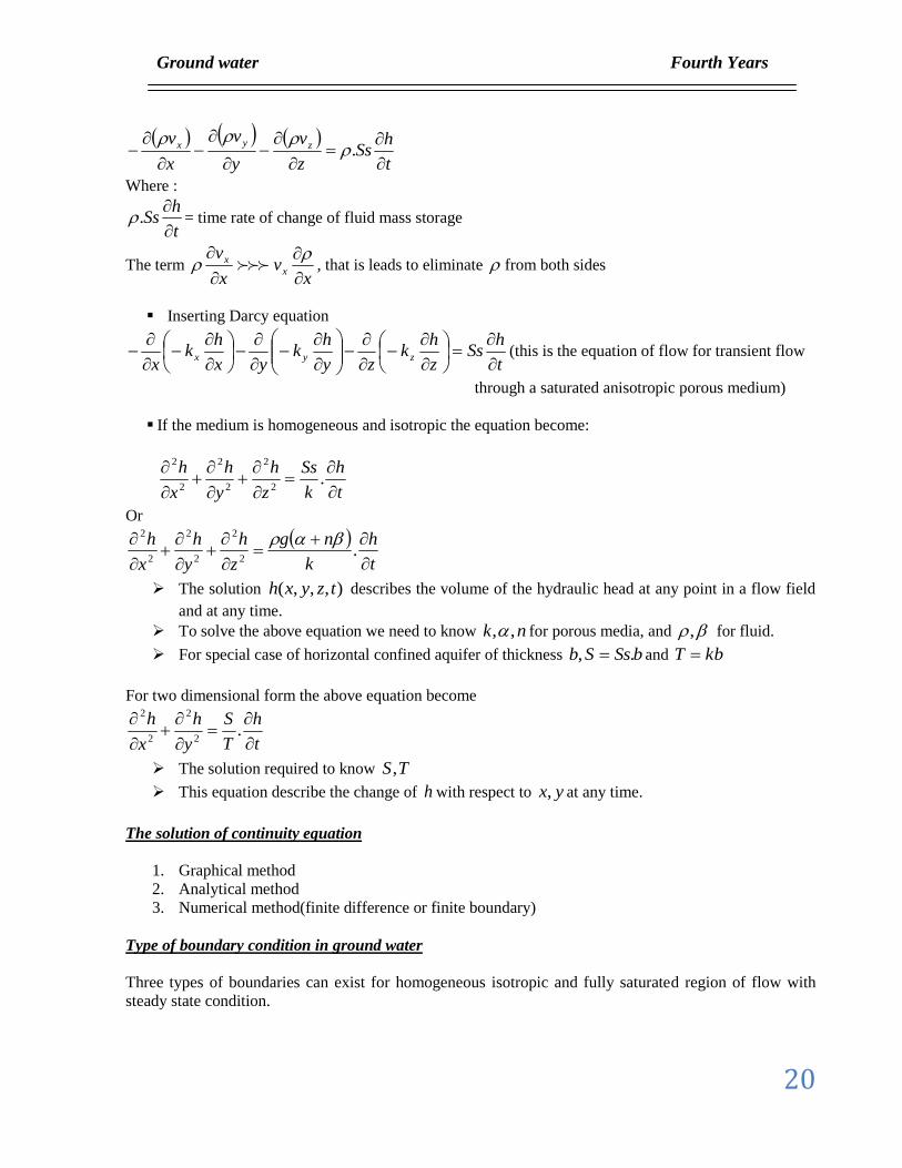
1. Impermeable boundaries (Neuman boundaries)
No flow across the boundaries
The flow lines adjacent to the boundary must be parallel to it.
The equipotential lines must meet the boundary at right angles
0
z
hThere is no flow across a flow line
0
x
h
By involving Darcy’s law and setting the specific discharge across the boundary equal to zero
00
x
h
x
hk
x
hkv
0
z
h
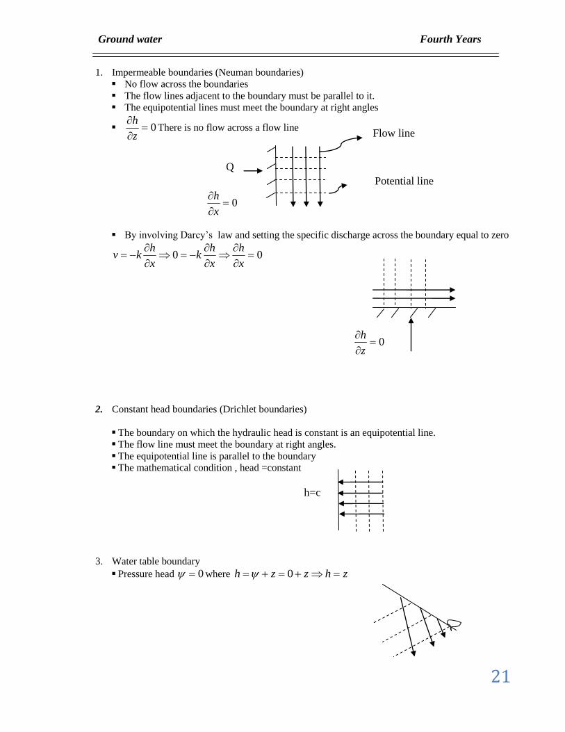
2. Constant head boundaries (Drichlet boundaries)
The boundary on which the hydraulic head is constant is an equipotential line.
The flow line must meet the boundary at right angles.
The equipotential line is parallel to the boundary
The mathematical condition , head =constant
3. Water table boundary
Pressure head 0 where zhzzh 0
Flow line
Potential line
Q
h=c
Ground water Fourth Years
22
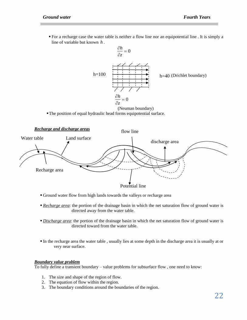
For a recharge case the water table is neither a flow line nor an equipotential line . It is simply a
line of variable but known h .
0
z
h
(Drichlet boundary)
0
z
h
(Neuman boundary)
The position of equal hydraulic head forms equipotential surface.
Recharge and discharge areas
Ground water flow from high lands towards the valleys or recharge area
Recharge area: the portion of the drainage basin in which the net saturation flow of ground water is
directed away from the water table.
Discharge area: the portion of the drainage basin in which the net saturation flow of ground water is
directed toward from the water table.
In the recharge area the water table , usually lies at some depth in the discharge area it is usually at or
very near surface.
Boundary value problem
To fully define a transient boundary – value problems for subsurface flow , one need to know:
1. The size and shape of the region of flow.
2. The equation of flow within the region.
3. The boundary conditions around the boundaries of the region.
h=100 h=40
Potential line
discharge area
flow line
Land surface Water table
Recharge area
Ground water Fourth Years
23
4. The initial condition of the region.
5. The spatial distribution of the hydraulic parameters that control the flow.
6. Mathematical method of solution.
If the boundary – value problem is for a steady – state system requirement (4) is removed.
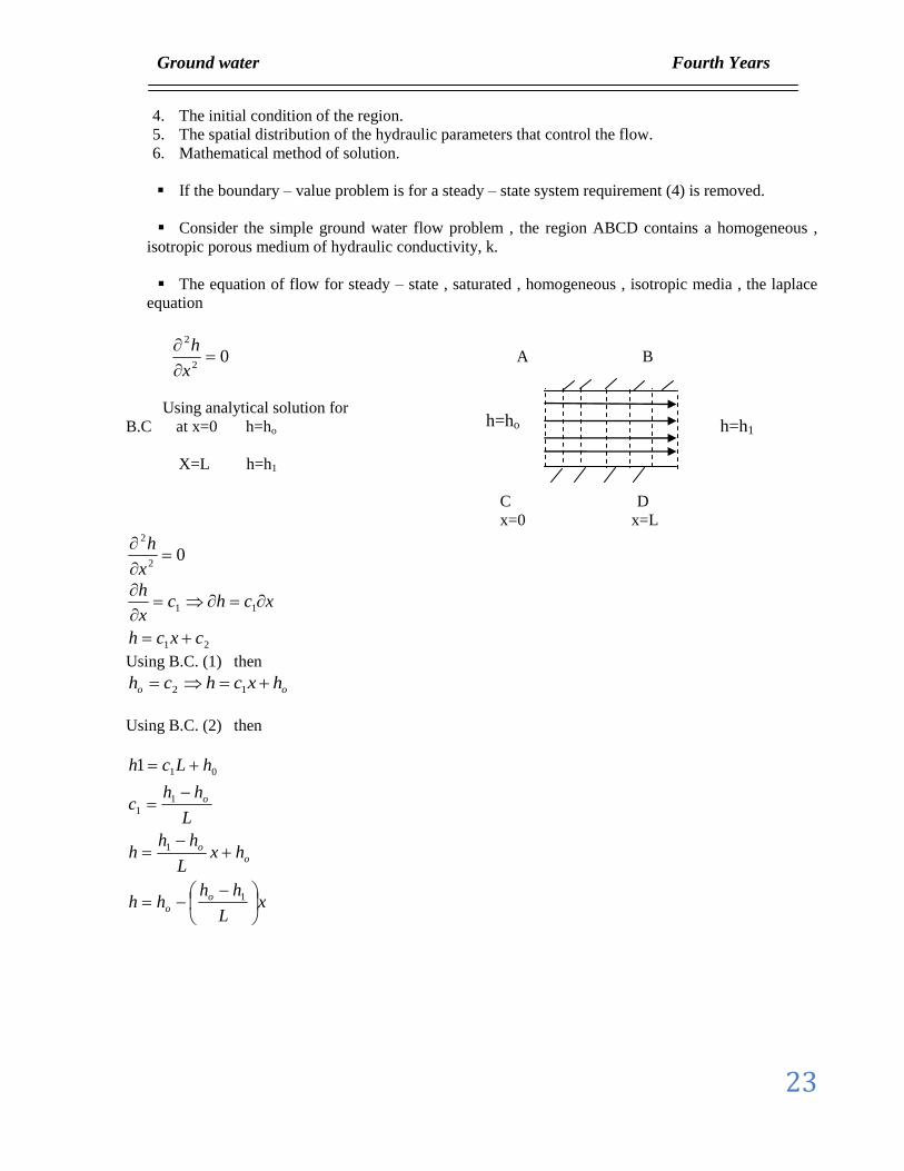
Consider the simple ground water flow problem , the region ABCD contains a homogeneous ,
isotropic porous medium of hydraulic conductivity, k.
The equation of flow for steady – state , saturated , homogeneous , isotropic media , the laplace
equation
02
2
x
h A B
Using analytical solution for
B.C at x=0 h=ho
X=L h=h1
C D
x=0 x=L
02
2
x
h
21
11
cxch
xchcx
h
Using B.C. (1) then
oo hxchch 12
Using B.C. (2) then
xL
hhhh
hxL
hhh
L
hhc
hLch
o
o
o
o
o
1
1
1
1
011
h=ho h=h1
Ground water Fourth Years
24
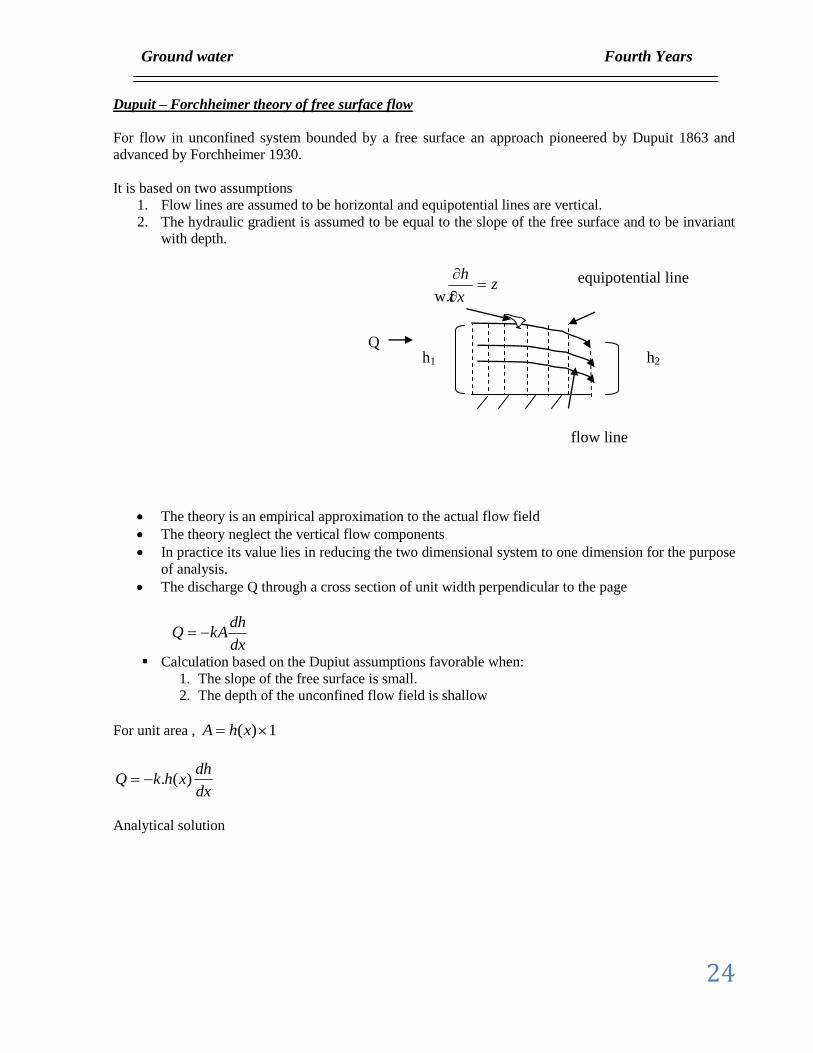
Dupuit – Forchheimer theory of free surface flow
For flow in unconfined system bounded by a free surface an approach pioneered by Dupuit 1863 and
advanced by Forchheimer 1930.
It is based on two assumptions
1. Flow lines are assumed to be horizontal and equipotential lines are vertical.
2. The hydraulic gradient is assumed to be equal to the slope of the free surface and to be invariant
with depth.
zx
h
The theory is an empirical approximation to the actual flow field
The theory neglect the vertical flow components
In practice its value lies in reducing the two dimensional system to one dimension for the purpose
of analysis.
The discharge Q through a cross section of unit width perpendicular to the page
dx
dhkAQ
Calculation based on the Dupiut assumptions favorable when:
1. The slope of the free surface is small.
2. The depth of the unconfined flow field is shallow
For unit area , 1)( xhA
dx
dhxhkQ )(.
Analytical solution
h1 h2
flow line
equipotential line
Q
w.t
Ground water Fourth Years
25
L
hhkQ
hhkQL
dhxhkdxQ
hh
hh
Lx
x
2
2
)(.
2
2
2
1
2
2
2
1
0
2
1
This equation is for unconfined flow
The equation of flow for Dupiut – Forchheimer theory in a homogeneous isotropic medium can be
developed from the continuity relationship
0
x
Q
This lead to 02
22
x
h
اذا كانunconfined فكلh تتحول الىh2hتتحول الى hلذلك نرجع الى االشتقاق ونعوض بدل
2
xL
hhhh
hxL
hhh
L
hhc
hLch
hhLx
hc
hhx
cxch
cx
h
2
2
2
12
1
2
1
2
1
2
22
2
1
2
21
2
11
2
2
2
2
12
1
21
2
1
2
@
0@
h is the head at any distance in unconfined system
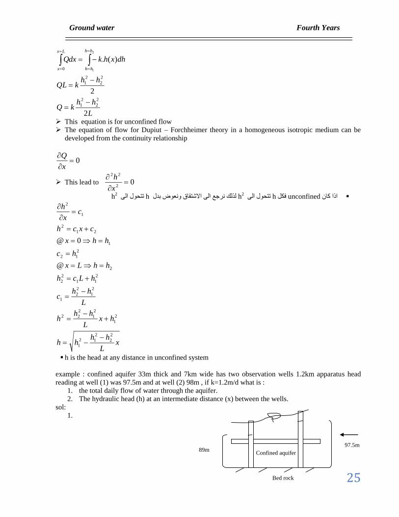
example : confined aquifer 33m thick and 7km wide has two observation wells 1.2km apparatus head
reading at well (1) was 97.5m and at well (2) 98m , if k=1.2m/d what is :
1. the total daily flow of water through the aquifer.
2. The hydraulic head (h) at an intermediate distance (x) between the wells.
sol:
1.
89m 97.5m
Bed rock
Confined aquifer
Ground water Fourth Years
26
dmQ
A
dx
dhkAQ
/5.19631200
895.97).700033(2.1
700033
3
2.
mh
h
25.93
600
5.97).700033(2.15.1963
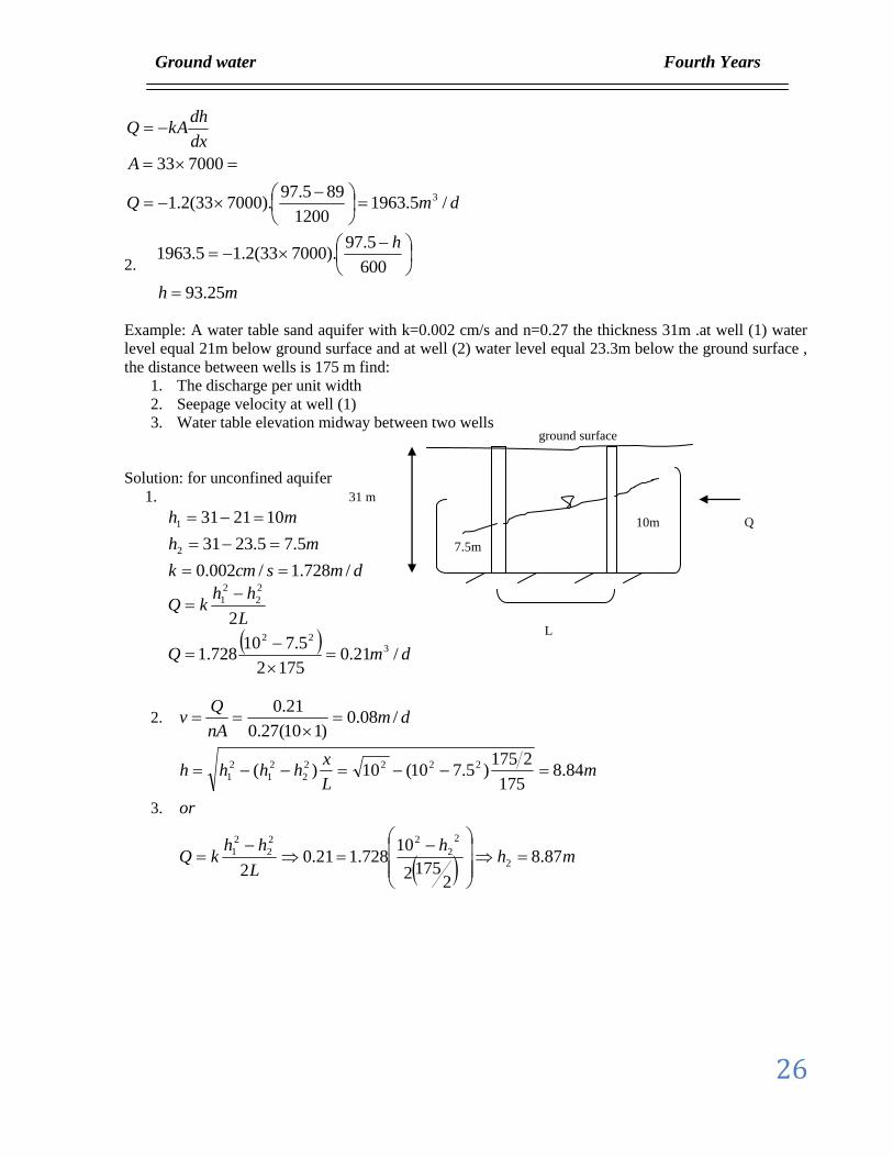
Example: A water table sand aquifer with k=0.002 cm/s and n=0.27 the thickness 31m .at well (1) water
level equal 21m below ground surface and at well (2) water level equal 23.3m below the ground surface ,
the distance between wells is 175 m find:
1. The discharge per unit width
2. Seepage velocity at well (1)
3. Water table elevation midway between two wells
Solution: for unconfined aquifer
1.
dmscmk
mh
mh
/728.1/002.0
5.75.2331
102131
2
1
dmQ
L
hhkQ
/21.01752
5.710728.1
2
322
2
2
2
1
2. dmnA
Qv /08.0
)110(27.0
21.0
3.
mh
h
L
hhkQ
or
mL
xhhhh
87.8
21752
10728.121.0
2
84.8175
2175)5.710(10)(
2
2
2
22
2
2
1
2222
2
2
1
2
1
7.5m
10m
L
ground surface
31 m
Q
Ground water Fourth Years
27
Drilling and Installation of wells and Piezometers
The selection depend on :
The purpose of the well
Hydrological environment
The quantity of water required
The depth and diameter required
Economic factor
Wells classified due to the method of construction:
1. Wells may be dug by hands
2. Driven in the form of well points
3. Bored by an earth auger or drilled by a drilling rig
There are three main types of drilling equipments
Cable tool
قة بالحبل ومن هذه االدوات طريقة بطيئة يحفر باالرتفاع لالعلى والنزول الى االسفل لمجموعة من االدوات والتي تكون معل
اداة الحفر Rotary
(drilling mud) طريقة سريعة وقليلة الكلفة )يحفر ويدفع سائل الحفر ومن ثم تعاد السوائل الى السطح ، يستخدم سائل يدعى
bentonitic clay in water مثل
Reverse rotary
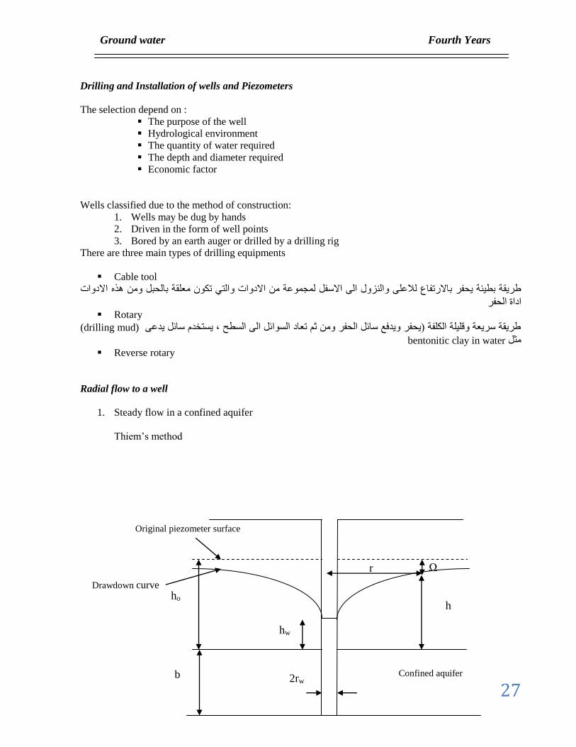
Radial flow to a well
1. Steady flow in a confined aquifer
Thiem’s method
ho
hw
b 2rw Confined aquifer
Original piezometer surface
Ω
h
Drawdown curve
r
Ground water Fourth Years
28
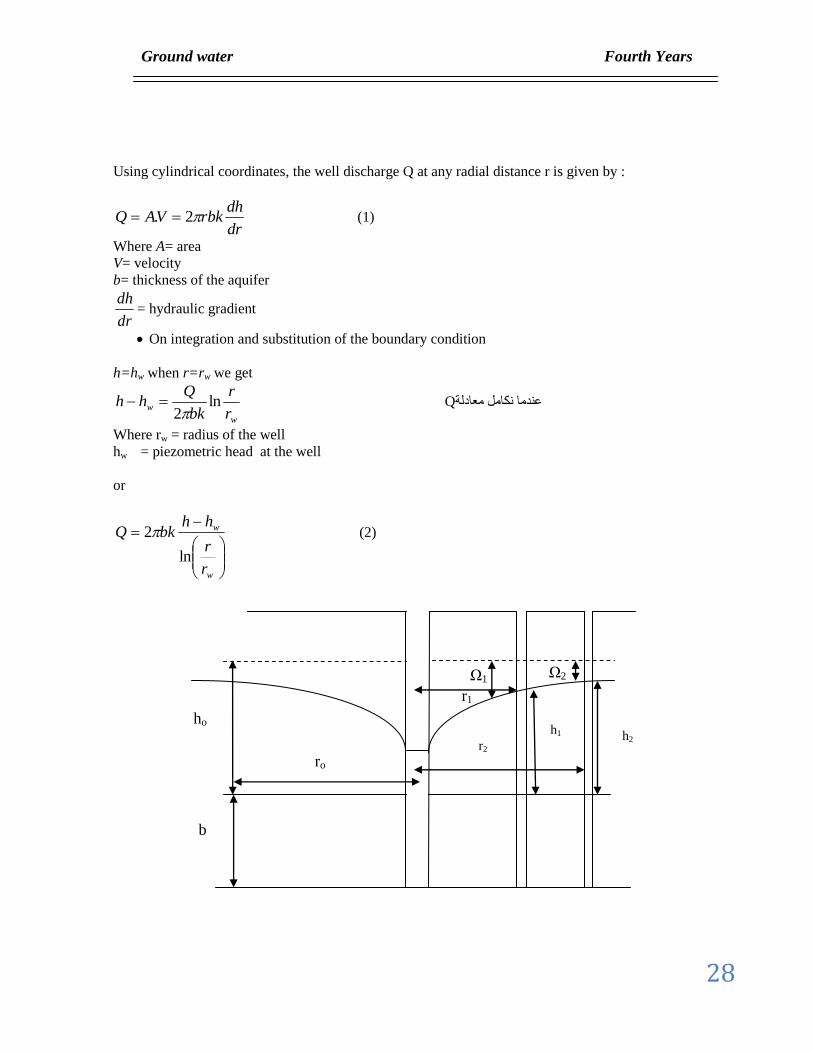
Using cylindrical coordinates, the well discharge Q at any radial distance r is given by :
dr
dhrbkVAQ 2. (1)
Where A= area
V= velocity
b= thickness of the aquifer
dr
dh= hydraulic gradient
On integration and substitution of the boundary condition
h=hw when r=rw we get
w
wr
r
bk
Qhh ln
2 Q عندما نكامل معادلة
Where rw = radius of the well
hw = piezometric head at the well
or
w
w
r
r
hhbkQ
ln
2 (2)
Ω1
ho
ro
b
h1
Ω2
r1
h2
r2
Ground water Fourth Years
29
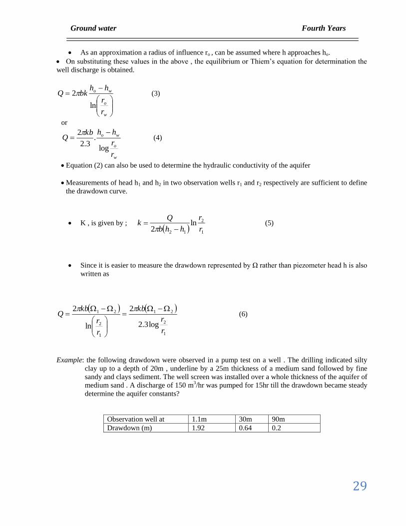
As an approximation a radius of influence ro , can be assumed where h approaches ho.
On substituting these values in the above , the equilibrium or Thiem’s equation for determination the
well discharge is obtained.
w
o
wo
r
r
hhbkQ
ln
2 (3)
or
w
o
wo
r
r
hhkbQ
log
.3.2
2
(4)
Equation (2) can also be used to determine the hydraulic conductivity of the aquifer
Measurements of head h1 and h2 in two observation wells r1 and r2 respectively are sufficient to define
the drawdown curve.
K , is given by ; 1
2
12
ln2 r
r
hhb
Qk
(5)
Since it is easier to measure the drawdown represented by Ω rather than piezometer head h is also
written as
1
2
21
1
2
21
log3.2
2
ln
2
r
r
kb
r
r
kbQ
(6)
Example: the following drawdown were observed in a pump test on a well . The drilling indicated silty
clay up to a depth of 20m , underline by a 25m thickness of a medium sand followed by fine
sandy and clays sediment. The well screen was installed over a whole thickness of the aquifer of
medium sand . A discharge of 150 m3/hr was pumped for 15hr till the drawdown became steady
determine the aquifer constants?
Observation well at 1.1m 30m 90m
Drawdown (m) 1.92 0.64 0.2
Ground water Fourth Years
30
Solution:
day
m
r
rQ
kb
day
m
day
hr
hr
mQ
3
21
1
2
33
14292.064.014.32
30
90log3.23600
2
log3.2.
360024150
The same procedure can be fallowed using other combinations of piezometers . the results are
given in the fallowing table.
r1(m) r2(m) Kb
1.1 30 1478.13
1.1 90 1465.55
30 90 1429
Σ=1457.5
K=1457.5/25=58.3 m/d≈58m/d
Or
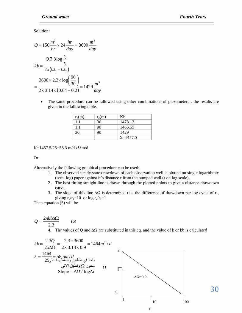
Alternatively the fallowing graphical procedure can be used:
1. The observed steady state drawdown of each observation well is plotted on single logarithmic
(semi log) paper against it’s distance r from the pumped well (r on log scale).
2. The best fitting straight line is drawn through the plotted points to give a distance drawdown
carve.
3. The slope of this line ∆Ω is determined (i.s. the difference of drawdown per log cycle of r ,
giving r2/r1=10 or log r2/r1=1
Then equation (5) will be
3.2
2
kbQ
(6)
4. The values of Q and ∆Ω are substituted in this eq. and the value of k or kb is calculated
dmk
dmQ
kb
/5.5825
1464
/14649.014.32
36003.2
2
3.2 2
2
1
0
10
100
1
∆Ω=0.9
Ω
r
لى ناخذ اي نقطتين ونسقطهما ع
ونطبق االتي Ωمحور
Slope = ∆Ω / log∆r
Ground water Fourth Years
31
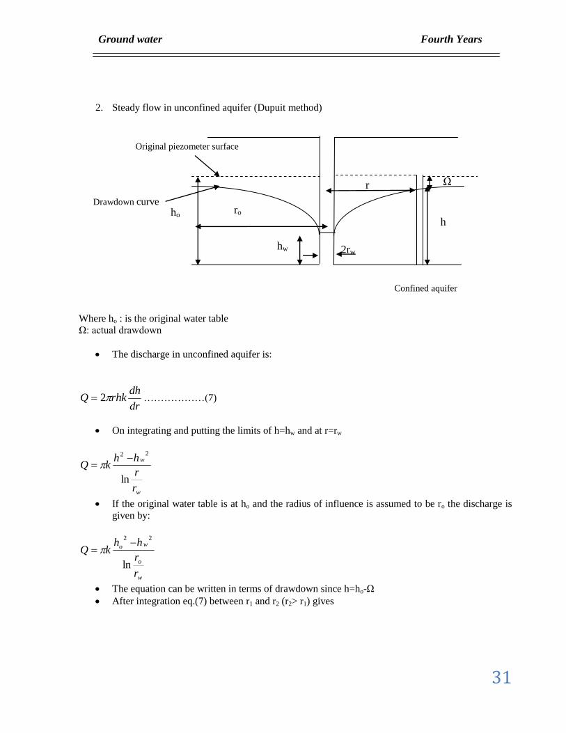
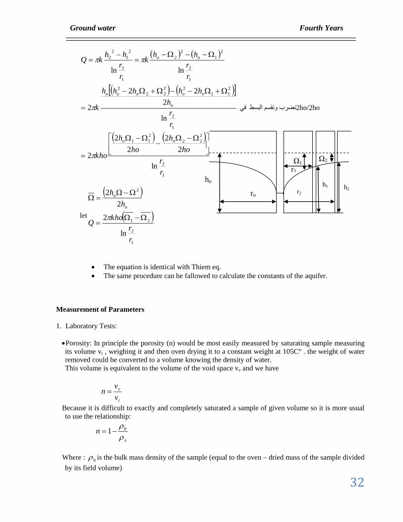
2. Steady flow in unconfined aquifer (Dupuit method)
Where ho : is the original water table
Ω: actual drawdown
The discharge in unconfined aquifer is:
dr
dhrhkQ 2 ………………(7)
On integrating and putting the limits of h=hw and at r=rw
w
w
r
r
hhkQ
ln
22
If the original water table is at ho and the radius of influence is assumed to be ro the discharge is
given by:
w
o
wo
r
r
hhkQ
ln
22
The equation can be written in terms of drawdown since h=ho-Ω
After integration eq.(7) between r1 and r2 (r2> r1) gives
Confined aquifer
ho
hw 2rw
Original piezometer surface
Ω
h
Drawdown curve
r
ro
Ground water Fourth Years
32
1
2
2
22
2
11
1
2
2
11
22
22
2
1
2
2
1
2
2
1
2
2
1
2
2
ln
2
2
2
2
2
ln
2
22
2
lnln
r
r
ho
h
ho
h
kho
r
r
h
hhhhh
k
r
r
hhk
r
r
hhkQ
oo
o
ooooo
oo
في البسط نضرب ونقسم 2ho/2ho
let
1
2
21
2
ln
2
2
2
r
r
khoQ
h
h
o
o
The equation is identical with Thiem eq.
The same procedure can be fallowed to calculate the constants of the aquifer.
Measurement of Parameters
1. Laboratory Tests:
Porosity: In principle the porosity (n) would be most easily measured by saturating sample measuring
its volume vt , weighing it and then oven drying it to a constant weight at 105C° . the weight of water
removed could be converted to a volume knowing the density of water.
This volume is equivalent to the volume of the void space vv and we have
t
v
v
vn
Because it is difficult to exactly and completely saturated a sample of given volume so it is more usual
to use the relationship:
s
bn
1
Where : b is the bulk mass density of the sample (equal to the oven – dried mass of the sample divided
by its field volume)
Ω1
ho
ro
h1
Ω2
r1
h2
r2
Ground water Fourth Years
33
s is the particle mass density ( the oven dried mass divided by the volume of solid particle) and it is
assumed for most mineral soils where great accuracy is not required equal to 2.65 g/ cm3
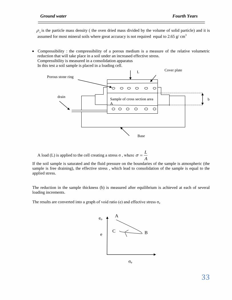
Compressibility : the compressibility of a porous medium is a measure of the relative volumetric
reduction that will take place in a soil under an increased effective stress.
Compressibility is measured in a consolidation apparatus
In this test a soil sample is placed in a loading cell.
A load (L) is applied to the cell creating a stress σ , where A
L
If the soil sample is saturated and the fluid pressure on the boundaries of the sample is atmospheric (the
sample is free draining), the effective stress , which lead to consolidation of the sample is equal to the
applied stress.
The reduction in the sample thickness (b) is measured after equilibrium is achieved at each of several
loading increments.
The results are converted into a graph of void ratio (e) and effective stress σe
A
B
C
eσ
e
eo
Sample of cross section area
A
Base
L
Porous stone ring
drain b
Cover plate
Ground water Fourth Years
34
Compressibility (α) is determined from the slope of the graph
e
e
o
d
bdb
d
ede
/
1
Where eo is the initial void ratio
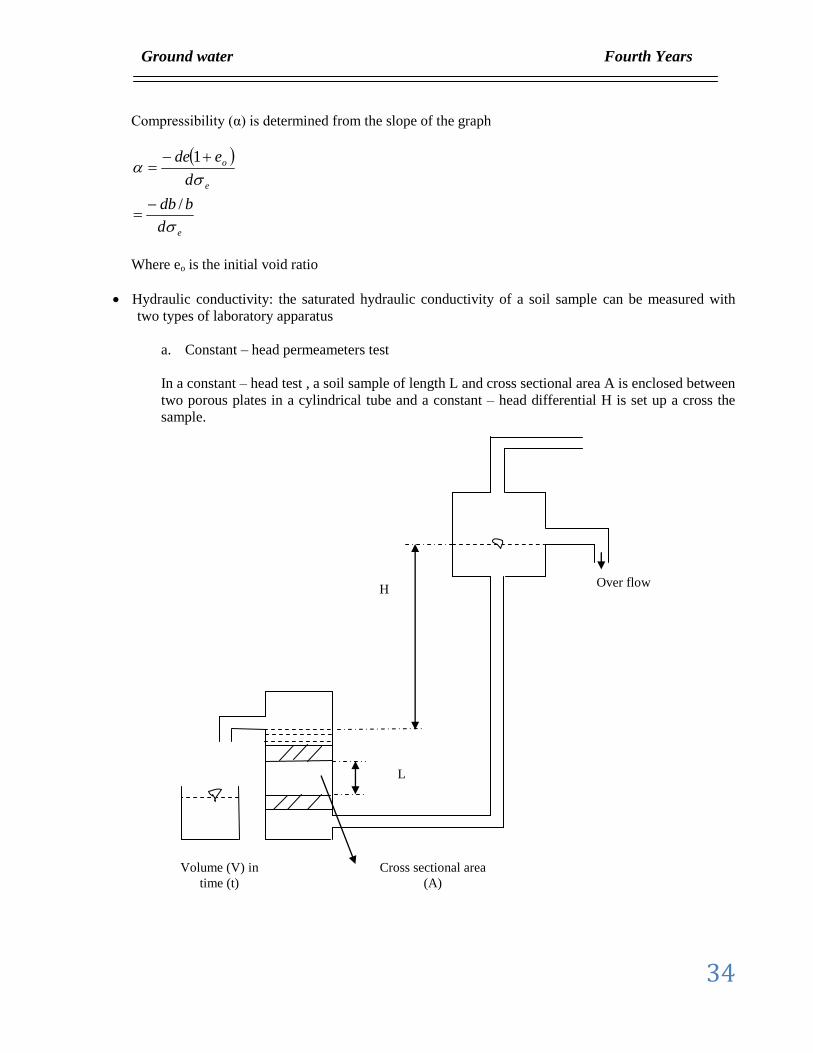
Hydraulic conductivity: the saturated hydraulic conductivity of a soil sample can be measured with
two types of laboratory apparatus
a. Constant – head permeameters test
In a constant – head test , a soil sample of length L and cross sectional area A is enclosed between
two porous plates in a cylindrical tube and a constant – head differential H is set up a cross the
sample.
Volume (V) in
time (t)
Cross sectional area
(A)
L
H Over flow
Ground water Fourth Years
35
L
HkAQ
A simple application of Darcy’s law lends to the expression
AH
QLk
where : Q is the steady volumetric discharge through the system
it is important that no air become entrapped in the system
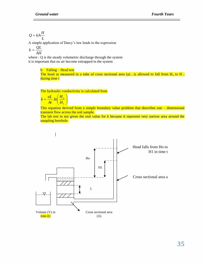
b. Falling – Head test
The head as measured in a tube of cross sectional area (a) , is allowed to fall from Ho to H 1
during time t
The hydraulic conductivity is calculated from
1
ln.H
H
At
aLk o
This equation derived from a simple boundary value problem that describes one – dimensional
transient flow across the soil sample.
The lab test in not given the real value for k because it represent very narrow area around the
sampling borehole.
Volume (V) in
time (t)
Cross sectional area
(A)
L
Ho
H1
Head falls from Ho to
H1 in time t
Cross sectional area a
Ground water Fourth Years
36
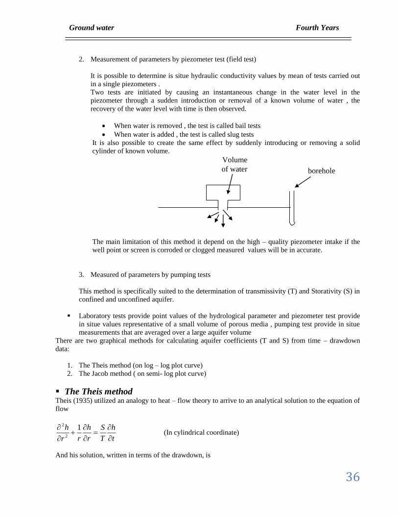
2. Measurement of parameters by piezometer test (field test)
It is possible to determine is situe hydraulic conductivity values by mean of tests carried out
in a single piezometers .
Two tests are initiated by causing an instantaneous change in the water level in the
piezometer through a sudden introduction or removal of a known volume of water , the
recovery of the water level with time is then observed.
When water is removed , the test is called bail tests
When water is added , the test is called slug tests
It is also possible to create the same effect by suddenly introducing or removing a solid
cylinder of known volume.
The main limitation of this method it depend on the high – quality piezometer intake if the
well point or screen is corroded or clogged measured values will be in accurate.
3. Measured of parameters by pumping tests
This method is specifically suited to the determination of transmissivity (T) and Storativity (S) in
confined and unconfined aquifer.
Laboratory tests provide point values of the hydrological parameter and piezometer test provide
in situe values representative of a small volume of porous media , pumping test provide in situe
measurements that are averaged over a large aquifer volume
There are two graphical methods for calculating aquifer coefficients (T and S) from time – drawdown
data:
1. The Theis method (on log – log plot curve)
2. The Jacob method ( on semi- log plot curve)
The Theis method Theis (1935) utilized an analogy to heat – flow theory to arrive to an analytical solution to the equation of
flow
t
h
T
S
r
h
rr
h
12
2
(In cylindrical coordinate)
And his solution, written in terms of the drawdown, is
borehole
Volume
of water
Ground water Fourth Years
37
Tt
Sr
u
ou
due
T
Qhh
4
2
.4
(1)
Where
ho = original hydraulic head
h = hydraulic head at any radial distance ,r
Ω = drawdown , is the difference between ho and h
Q = steady pumping rate
T = Transmisivity
S = Storativity
Where Tt
Sru
4
2
Equation (1) can be written : )(.4
uwT
Q
W(u) = the well function of u
The values of the integral w (u) can be tabulated for each of the several values of u as can be seen in
table(1).
Example : a well is located in an aquifer with a conductivity of 15 m/d and S=0.005 . The aquifer is 20m
thick and is pumped at a rate of 2725m3/d , what is drawdown Ω at a distance 7m from the well after one
day of pumping.
Sol:
muwT
Q
uwuattablefrom
tT
Sru
dmbkT
74.53004
94.72725)(.
4
94.7)(102
0002.013004
005.07
.4
.
/3002015.
4
22
3
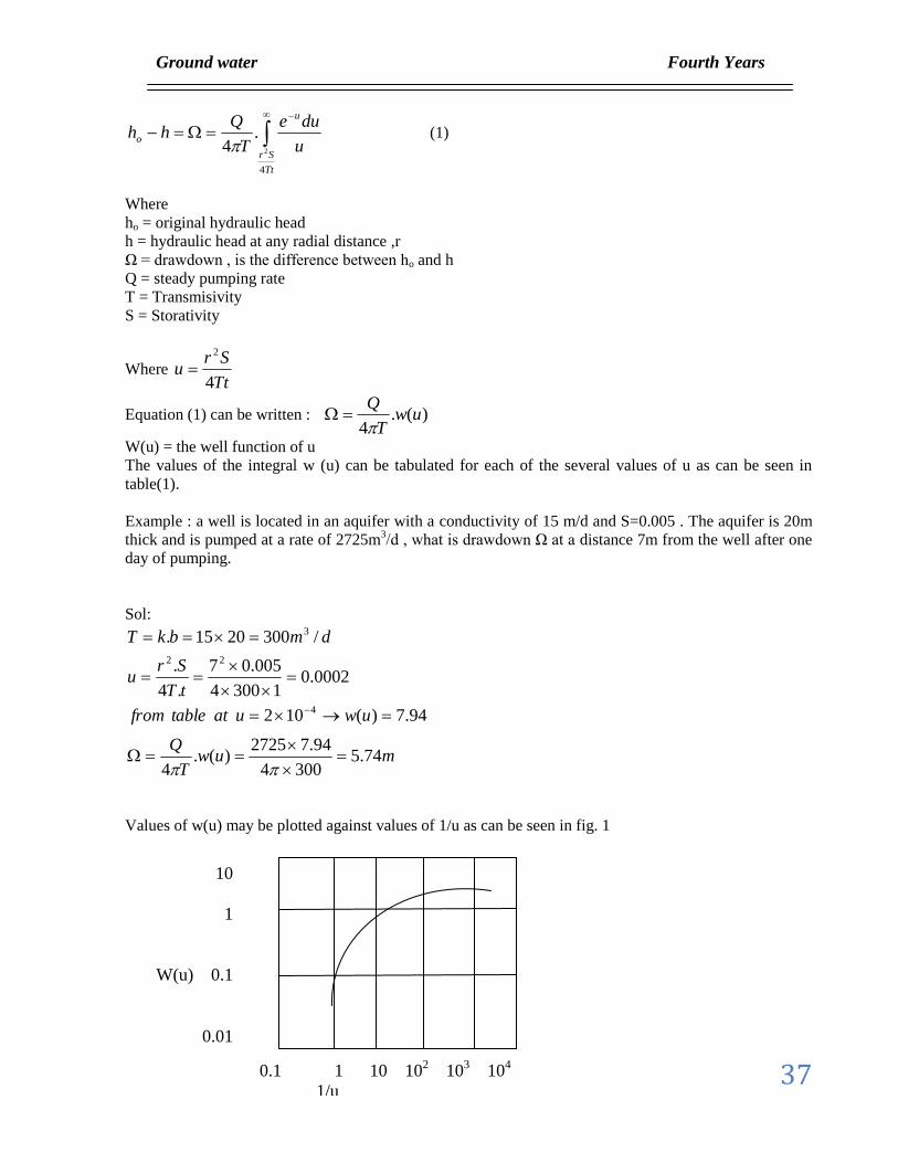
Values of w(u) may be plotted against values of 1/u as can be seen in fig. 1
10
1
W(u) 0.1
0.01
0.1 1 10 102 10
3 10
4
1/u
Ground water Fourth Years
38
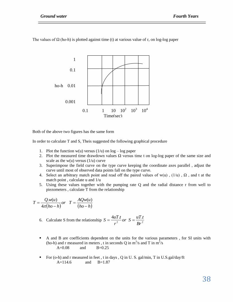
The values of Ω (ho-h) is plotted against time (t) at various value of r, on log-log paper
Both of the above two figures has the same form
In order to calculate T and S, Theis suggested the following graphical procedure
1. Plot the function w(u) versus (1/u) on log – log paper
2. Plot the measured time drawdown values Ω versus time t on log-log paper of the same size and
scale as the w(u) versus (1/u) curve
3. Superimpose the field curve on the type curve keeping the coordinate axes parallel , adjust the
curve until most of observed data points fall on the type curve.
4. Select an arbitrary match point and read off the paired values of w(u) , (1/u) , Ω , and t at the
match point , calculate u and 1/u
5. Using these values together with the pumping rate Q and the radial distance r from well to
piezometers , calculate T from the relationship
hho
uAQwTor
hho
uwQT
)(
4
)(.
6. Calculate S from the relationship 22
..4
Br
tuTSor
r
tuTS
A and B are coefficients dependent on the units for the various parameters , for SI units with
(ho-h) and r measured in meters , t in seconds Q in m3/s and T in m
2/s
A=0.08 and B=0.25
For (o-h) and r measured in feet , t in days , Q in U. S. gal/min, T in U.S.gal/day/ft
A=114.6 and B=1.87
1
0.1
ho-h 0.01
0.001
0.1 1 10 102 10
3 10
4
Time(sec)
Ground water Fourth Years
39
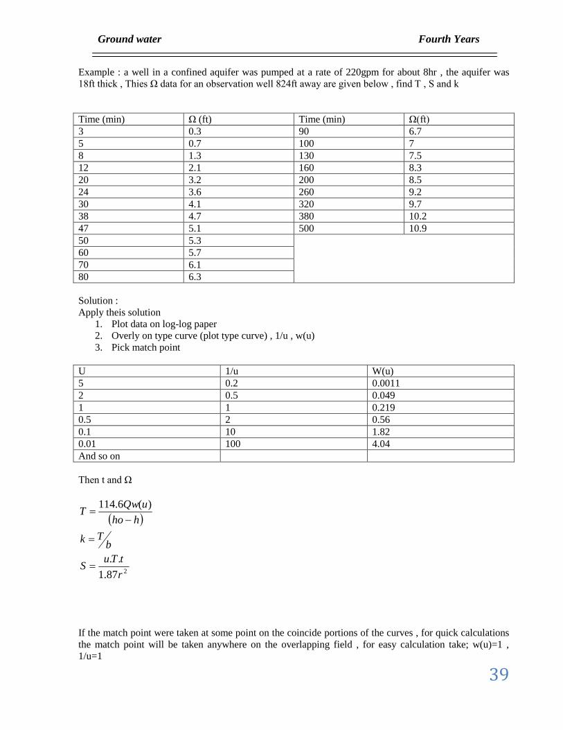
Example : a well in a confined aquifer was pumped at a rate of 220gpm for about 8hr , the aquifer was
18ft thick , Thies Ω data for an observation well 824ft away are given below , find T , S and k
Time (min) Ω (ft) Time (min) Ω(ft)
3 0.3 90 6.7
5 0.7 100 7
8 1.3 130 7.5
12 2.1 160 8.3
20 3.2 200 8.5
24 3.6 260 9.2
30 4.1 320 9.7
38 4.7 380 10.2
47 5.1 500 10.9
50 5.3
60 5.7
70 6.1
80 6.3
Solution :
Apply theis solution
1. Plot data on log-log paper
2. Overly on type curve (plot type curve) , 1/u , w(u)
3. Pick match point
U 1/u W(u)
5 0.2 0.0011
2 0.5 0.049
1 1 0.219
0.5 2 0.56
0.1 10 1.82
0.01 100 4.04
And so on
Then t and Ω
287.1
..
)(6.114
r
tTuS
bTk
hho
uQwT
If the match point were taken at some point on the coincide portions of the curves , for quick calculations
the match point will be taken anywhere on the overlapping field , for easy calculation take; w(u)=1 ,
1/u=1
Ground water Fourth Years
40
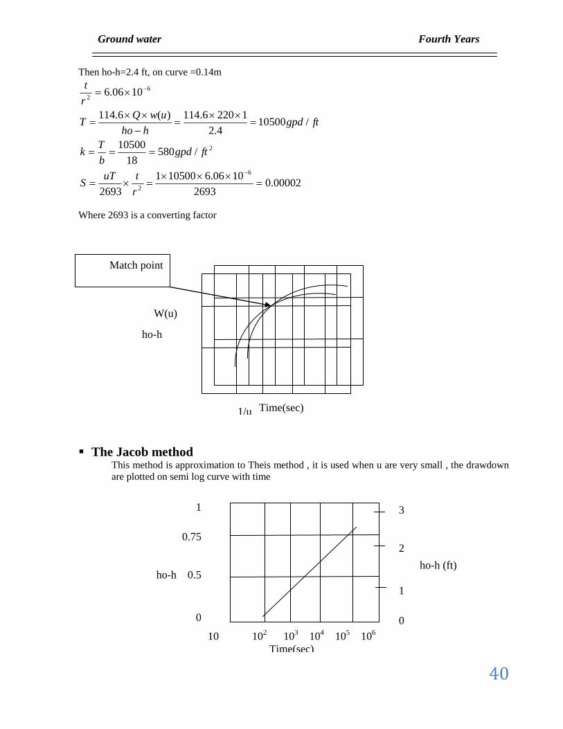
Then ho-h=2.4 ft, on curve =0.14m
00002.02693
1006.6105001
2693
/58018
10500
/105004.2
12206.114)(6.114
1006.6
6
2
2
6
2
r
tuTS
ftgpdb
Tk
ftgpdhho
uwQT
r
t
Where 2693 is a converting factor
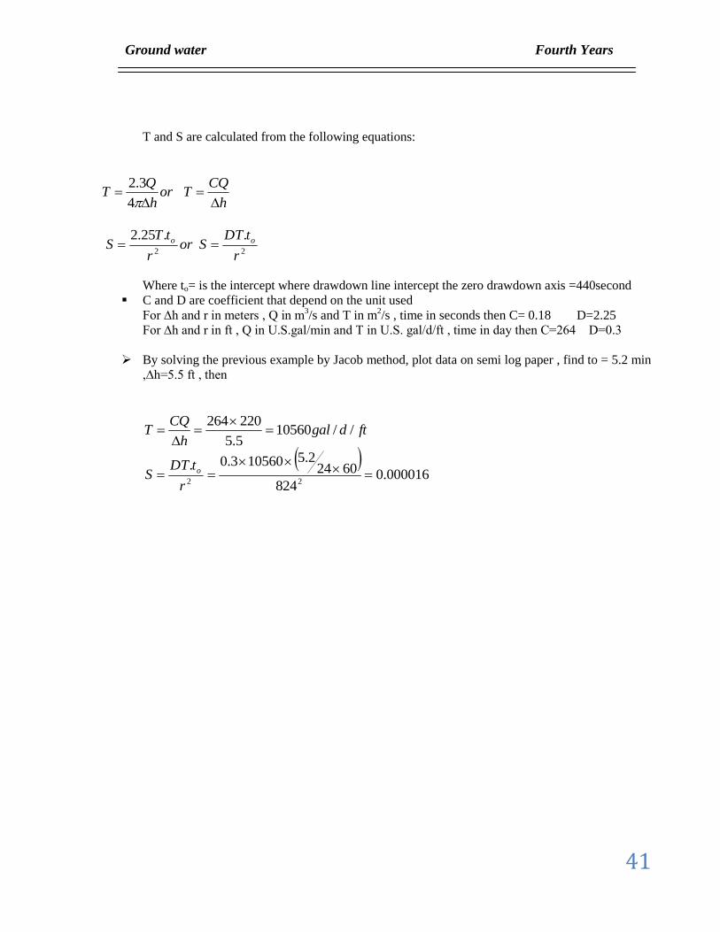
The Jacob method This method is approximation to Theis method , it is used when u are very small , the drawdown
are plotted on semi log curve with time
W(u)
1/u
ho-h
Time(sec)
Match point
1
0.75
ho-h 0.5
0
10 102 10
3 10
4 10
5 10
6
Time(sec)
3
2
ho-h (ft)
1
0
Ground water Fourth Years
41
T and S are calculated from the following equations:
h
CQTor
h
QT
4
3.2
22
..25.2
r
tDTSor
r
tTS oo
Where to= is the intercept where drawdown line intercept the zero drawdown axis =440second
C and D are coefficient that depend on the unit used
For ∆h and r in meters , Q in m3/s and T in m
2/s , time in seconds then C= 0.18 D=2.25
For ∆h and r in ft , Q in U.S.gal/min and T in U.S. gal/d/ft , time in day then C=264 D=0.3
By solving the previous example by Jacob method, plot data on semi log paper , find to = 5.2 min
,∆h=5.5 ft , then
ftdgalh
CQT //10560
5.5
220264
000016.0
824
60242.5105603.0.
22
r
tDTS o

Ground water Fourth Years
42
Ground Water Contamination
A ground water contamination is defined by most regulatory agencies as any physical, chemical,
biological or radiological substance or matter in ground water.
The contaminations can be introduced in the ground water by naturally accruing activities, such as
natural leaching of soil and other material with ground water.
Or ground water contamination can be introduced by human activities such as waste disposal,
agricultural operations; human activities are the leading cause of ground water contamination.
Sources of contamination 1. land disposal of solid waste
Leaching of dissolved solid contaminates to ground water by percolating water derived from rain or
snowmelt (the liquid called leachate).
Leachate from sanitary land fill contains large number of inorganic contaminates, organic
contaminates and large amount of dissolved solid.
In industrial disposal site leachate may contains toxic constituents from liquid industrial waste
placed in landfill.
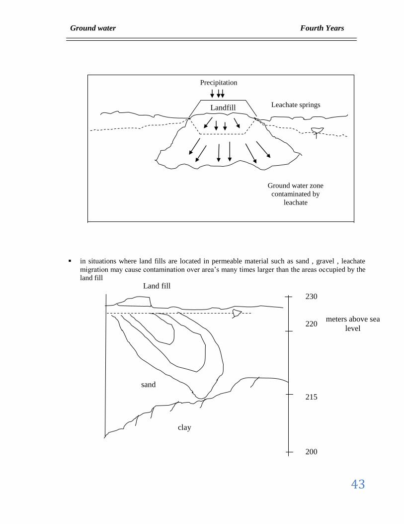
Downward flow of leachate may threaten ground water outward flow causing leachate springs or
seepage into streams or other surface water bodies.
land disposal of solid waste
domestic sanitary landfill; solid waste is
reduced in volume by compaction and then
covered with earth , the landfill consisting of
successive layers of compacted waste and
earth may by constructed on the ground
surface in excavation
industrial disposal site
Ground water Fourth Years
43
in situations where land fills are located in permeable material such as sand , gravel , leachate
migration may cause contamination over area’s many times larger than the areas occupied by the
land fill
Precipitation
Landfill Leachate springs
Ground water zone
contaminated by
leachate
Land fill
sand
clay
230
220
215
200
meters above sea
level
Ground water Fourth Years
44
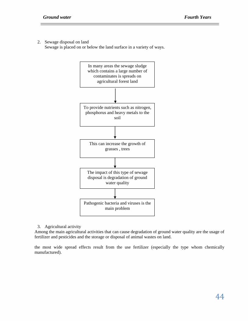
2. Sewage disposal on land
Sewage is placed on or below the land surface in a variety of ways.
3. Agricultural activity
Among the main agricultural activities that can cause degradation of ground water quality are the usage of
fertilizer and pesticides and the storage or disposal of animal wastes on land.
the most wide spread effects result from the use fertilizer (especially the type whom chemically
manufactured).
In many areas the sewage sludge
which contains a large number of
contaminates is spreads on
agricultural forest land
To provide nutrients such as nitrogen,
phosphorus and heavy metals to the
soil
This can increase the growth of
grasses , trees
The impact of this type of sewage
disposal is degradation of ground
water quality
Pathogenic bacteria and viruses is the
main problem
Ground water Fourth Years
45
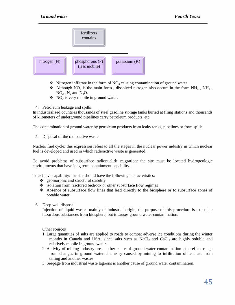
Nitrogen infiltrate in the form of NO3 causing contamination of ground water.
Although NO3 is the main form , dissolved nitrogen also occurs in the form NH4 , NH3 ,
NO2 , N2 and N2O.
NO3 is very mobile in ground water.
4. Petroleum leakage and spills
In industrialized countries thousands of steel gasoline storage tanks buried at filing stations and thousands
of kilometers of underground pipelines carry petroleum products, etc.
The contamination of ground water by petroleum products from leaky tanks, pipelines or from spills.
5. Disposal of the radioactive waste
Nuclear fuel cycle: this expression refers to all the stages in the nuclear power industry in which nuclear
fuel is developed and used in which radioactive waste is generated.
To avoid problems of subsurface radionuclide migration: the site must be located hydrogeologic
environments that have long term containment capability.
To achieve capability: the site should have the following characteristics:
geomorphic and structural stability
isolation from fractured bedrock or other subsurface flow regimes
Absence of subsurface flow lines that lead directly to the biosphere or to subsurface zones of
potable water.
6. Deep well disposal
Injection of liquid wastes mainly of industrial origin, the purpose of this procedure is to isolate
hazardous substances from biosphere, but it causes ground water contamination.
Other sources
1. Large quantities of salts are applied to roads to combat adverse ice conditions during the winter
months in Canada and USA, since salts such as NaCl2 and CaCl2 are highly soluble and
relatively mobile in ground water.
2. Activity of mining industry are another cause of ground water contamination , the effect range
from changes in ground water chemistry caused by mining to infiltration of leachate from
tailing and another wastes.
3. Seepage from industrial waste lagoons is another cause of ground water contamination.
fertilizers
contains
nitrogen (N)
phosphorous (P)
(less mobile)
potassium (K)
Ground water Fourth Years
46
Source of ground water contamination: a contaminate is any dissolved solute or non aqueous liquid
that inters ground water as a consequence of people’s activities
Types of contaminates sources
a. Continuous: leakage from underground storage tank.
b. Discontinuous: Instantaneous or slug spill from quick spill or ruptured underground tank.
Other representation is:
1. point source
2. line source
3. area source
Type's contaminants
reactive
nonreactive
dissolved
non dissolved (immiscible in water oil and gasoline)
Transport Processes
The common starting point in the development of differential equation to describe the transport of solutes
in porous materials is to consider the flux of solute into and out of a fixed elemental volume within the
flow domain.
A conservative of mass
Net rate of change of mass of solute within the element=
Flux of solute into - flux of solute out of ± loss or gain of solute mass due to reactions
The element the element
After solving this equation
The physical processes that control the flux in and out of the elemental volume are advection and
hydrodynamic dispersion.
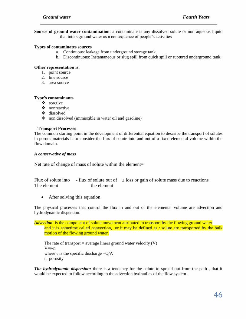
Advection: is the component of solute movement attributed to transport by the flowing ground water
and it is sometime called convection, or it may be defined as : solute are transported by the bulk
motion of the flowing ground water.
The rate of transport = average liners ground water velocity (V)
V=v/n
where v is the specific discharge =Q/A
n=porosity
The hydrodynamic dispersion: there is a tendency for the solute to spread out from the path , that it
would be expected to follow according to the advection hydraulics of the flow system .
Ground water Fourth Years
47
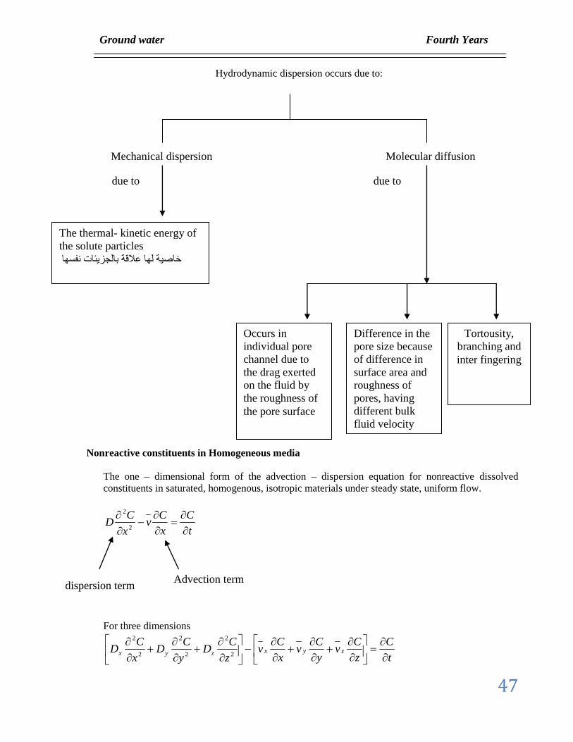
Hydrodynamic dispersion occurs due to:
Nonreactive constituents in Homogeneous media
The one – dimensional form of the advection – dispersion equation for nonreactive dissolved
constituents in saturated, homogenous, isotropic materials under steady state, uniform flow.
t
C
x
Cv
x
CD
2
2
For three dimensions
t
C
z
Cv
y
Cv
x
Cv
z
CD
y
CD
x
CD zyxzyx
2
2
2
2
2
2
Mechanical dispersion Molecular diffusion
due to due to
The thermal- kinetic energy of
the solute particles
خاصية لها عالقة بالجزيئات نفسها
Tortousity,
branching and
inter fingering
Difference in the
pore size because
of difference in
surface area and
roughness of
pores, having
different bulk
fluid velocity
Occurs in
individual pore
channel due to
the drag exerted
on the fluid by
the roughness of
the pore surface
dispersion term Advection term
Ground water Fourth Years
48
Where D= coefficient of hydrodynamic dispersion,
D= molecular diffusion + mechanical dispersion =Dd+Dm
vDm
where : characteristic property of the porous medium known as dispersivity (L)
v : ground water velocity
od DD
where : tortuosity factor (0.6- 0.7)
oD : free solute diffusion (from tables)
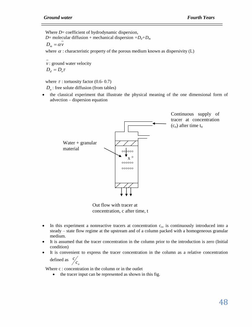
the classical experiment that illustrate the physical meaning of the one dimensional form of
advection – dispersion equation
In this experiment a nonreactive tracers at concentration co, is continuously introduced into a
steady – state flow regime at the upstream and of a column packed with a homogeneous granular
medium.
It is assumed that the tracer concentration in the column prior to the introduction is zero (Initial
condition)
It is convenient to express the tracer concentration in the column as a relative concentration
defined as oc
c
Where c : concentration in the column or in the outlet
the tracer input can be represented as shown in this fig.
Continuous supply of
tracer at concentration
(co) after time to
°°°°°°
°x
°°°°°°
°°°°°°
°
Water + granular
material
Out flow with tracer at
concentration, c after time, t
Ground water Fourth Years
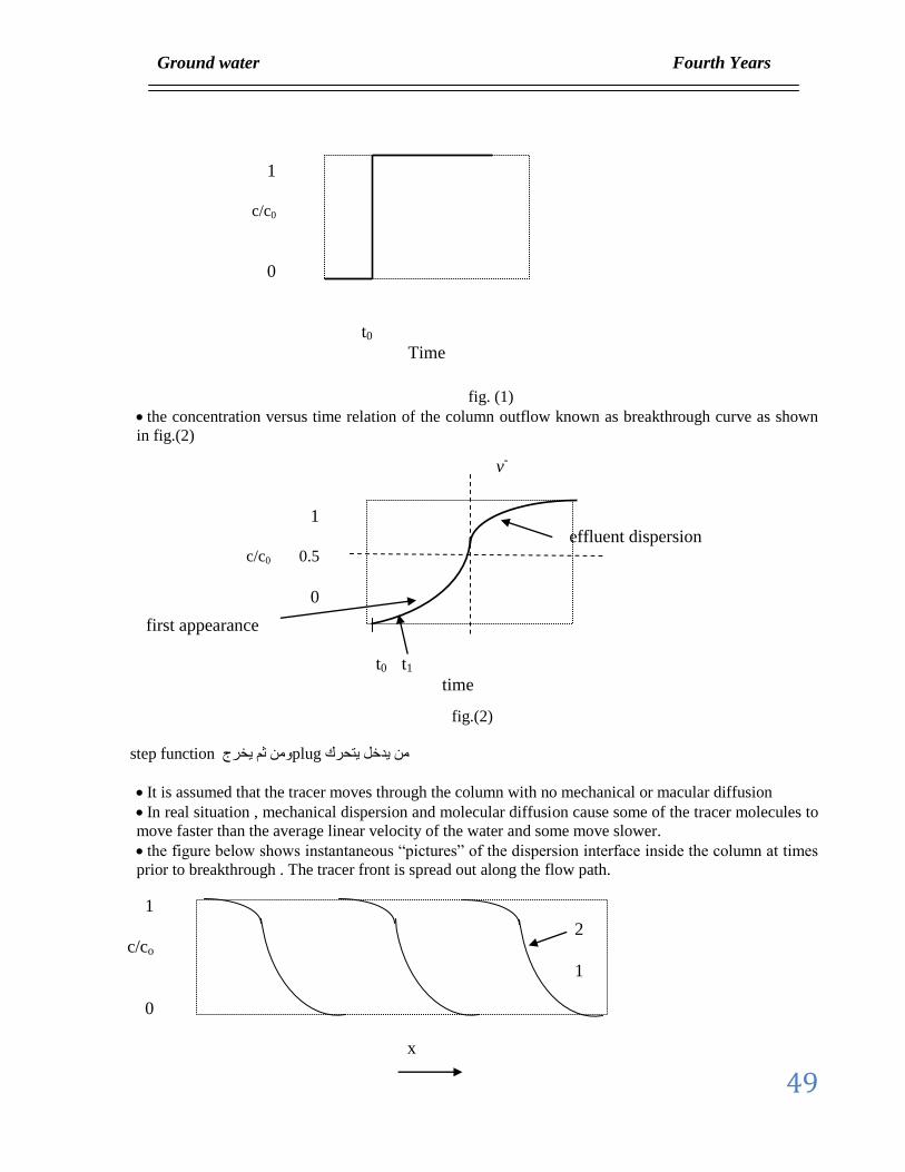
49
fig. (1)
the concentration versus time relation of the column outflow known as breakthrough curve as shown
in fig.(2)
fig.(2)
step function ومن ثم يخرجplug من يدخل يتحرك
It is assumed that the tracer moves through the column with no mechanical or macular diffusion
In real situation , mechanical dispersion and molecular diffusion cause some of the tracer molecules to
move faster than the average linear velocity of the water and some move slower.
the figure below shows instantaneous “pictures” of the dispersion interface inside the column at times
prior to breakthrough . The tracer front is spread out along the flow path.
1
c/c0
0
t0
Time
1
c/c0 0.5
0
t0 t1
time
v-
effluent dispersion
first appearance
x
1
c/co
0
2
1
Ground water Fourth Years
50
لوثات مستمر لمسافات متعددة من العموداندفاع الم
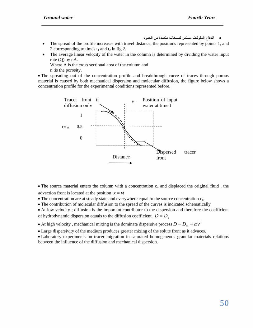
The spread of the profile increases with travel distance, the positions represented by points 1, and
2 corresponding to times t1 and t2 in fig.2.
The average linear velocity of the water in the column is determined by dividing the water input
rate (Q) by nA.
Where A is the cross sectional area of the column and
n ;is the porosity.
The spreading out of the concentration profile and breakthrough curve of traces through porous
material is caused by both mechanical dispersion and molecular diffusion, the figure below shows a
concentration profile for the experimental conditions represented before.
The source material enters the column with a concentration co and displaced the original fluid , the
advection front is located at the position tvx
The concentration are at steady state and everywhere equal to the source concentration co.
The contribution of molecular diffusion to the spread of the curves is indicated schematically
At low velocity ; diffusion is the important contributor to the dispersion and therefore the coefficient
of hydrodynamic dispersion equals to the diffusion coefficient. dDD
At high velocity , mechanical mixing is the dominate dispersive process vDD m
Large dispersivity of the medium produces greater mixing of the solute front as it advaces.
Laboratory experiments on tracer migration in saturated homogeneous granular materials relations
between the influence of the diffusion and mechanical dispersion.
1
c/c0 0.5
0
Distance
v-
Dispersed tracer
front
Position of input
water at time t
Tracer front if
diffusion only
Ground water Fourth Years
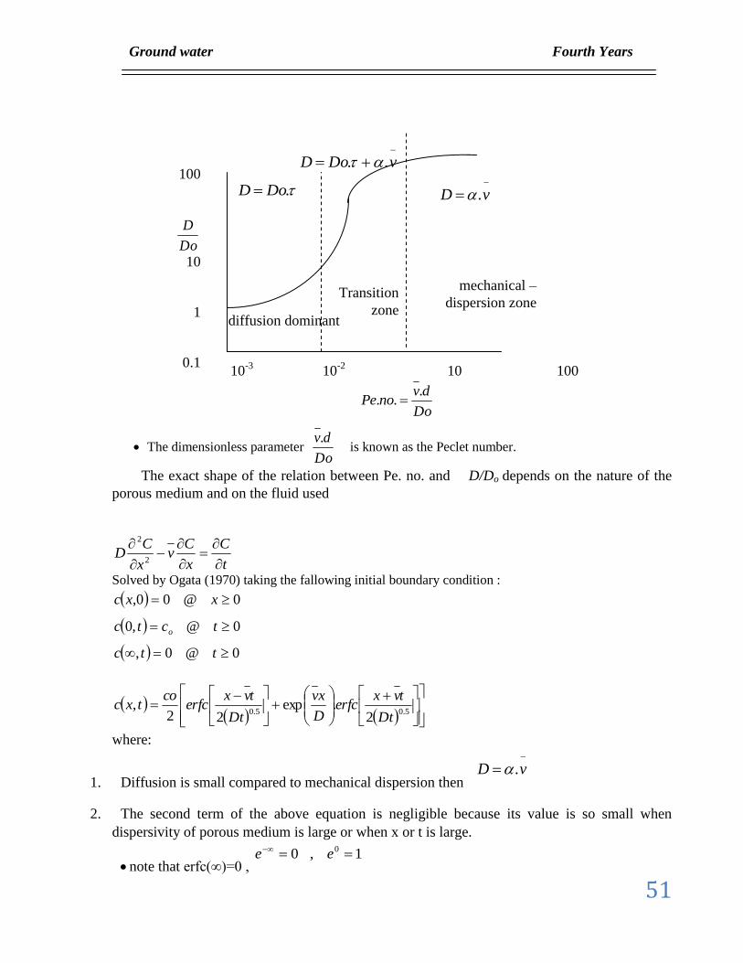
51
The dimensionless parameter Do
dv.
is known as the Peclet number.
The exact shape of the relation between Pe. no. and D/Do depends on the nature of the
porous medium and on the fluid used
t
C
x
Cv
x
CD
2
2
Solved by Ogata (1970) taking the fallowing initial boundary condition :
0@0,
0@,0
0@00,
ttc
tctc
xxc
o
5.05.02
.exp22
,Dt
tvxerfc
D
xv
Dt
tvxerfc
cotxc
where:
1. Diffusion is small compared to mechanical dispersion then
vD .
2. The second term of the above equation is negligible because its value is so small when
dispersivity of porous medium is large or when x or t is large.
note that erfc(∞)=0 , 1,0 0 ee
100
Do
D
10
1
0.1 10
-3 10
-2 10 100
Do
dvnoPe
...
diffusion dominant
Transition
zone
mechanical –
dispersion zone
vDoD ..
vD .
.DoD
Ground water Fourth Years
52
Then we get
5.02
.2
1
Dt
tvxerfc
c
c
o
where : erfc = complementary error function
)(1)(
)(
)(1)(
BerfBerfc
BerfBerf
BerfBerfc
5.0
2 tv
tvxB
From table (1) , B , erf(B) , erfc(B)
If we know B we know erfc(B) , and if we know erfc (B) , we know B
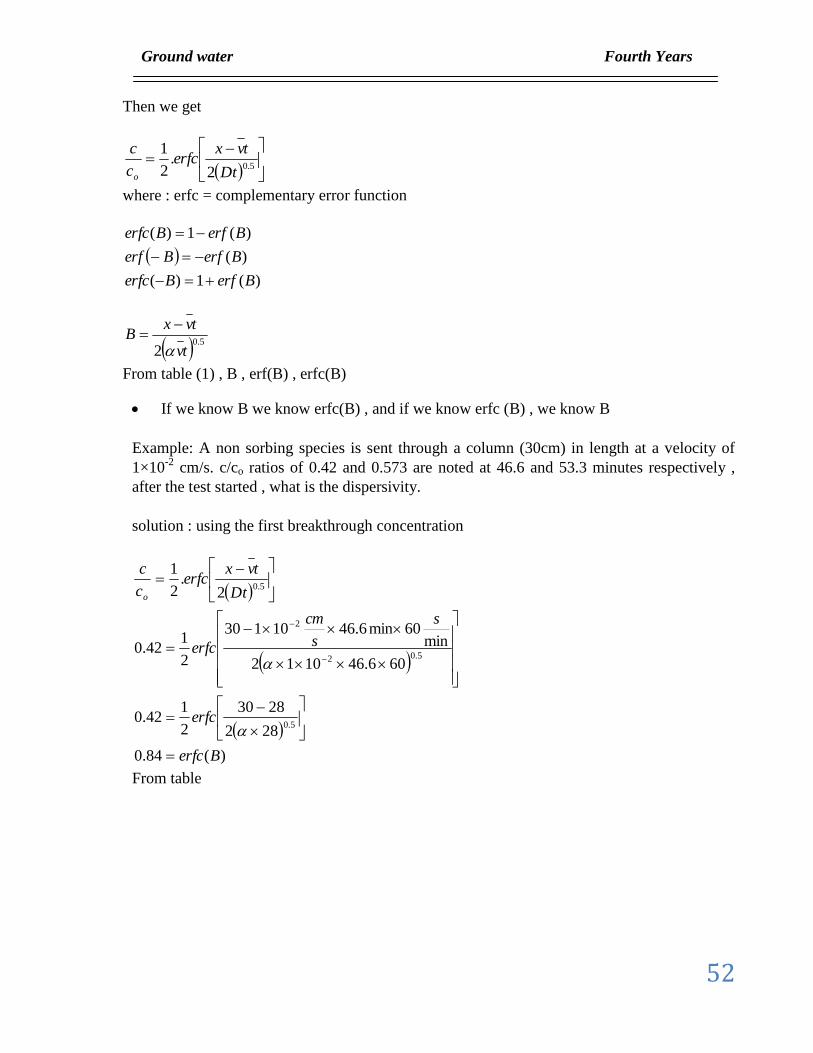
Example: A non sorbing species is sent through a column (30cm) in length at a velocity of
1×10⁻²
cm/s. c/co ratios of 0.42 and 0.573 are noted at 46.6 and 53.3 minutes respectively ,
after the test started , what is the dispersivity.
solution : using the first breakthrough concentration
)(84.0
282
2830
2
142.0
606.461012
min60min6.4610130
2
142.0
2.
2
1
5.0
5.02
2
5.0
Berfc
erfc
s
s
cm
erfc
Dt
tvxerfc
c
c
o
From table
Ground water Fourth Years
53
BX
X
X
x
x
xx
yy
xx
yy
14.0
1093015.7055533.0
105533.5055533.01037685.2
05.0
055533.0
1.0
047537.0
1.015.0
887537.0832004.0
1.0
887537.084.0
3
33
12
12
1
1
Substitute in the equation
8.1
282
214.0
282
283014.0
5.0
The second calculation is the same
146.0
1146.1)(
)(1146.1
)(1)(146.1
322
2146.1
322
3230
2
1573.0
603.531012
603.5310130
2
1573.0
5.02
2
Berf
Berf
BerfBerfc
erfc
erfc
erfc
From table
BX
X
x
x
xx
yy
xx
yy
13.0
105533.5055533.01067685.1
05.0
055533.0
1.0
033537.0
1.015.0
112463.0167996.0
1.0
112463.0146.0
33
12
12
1
1
8.1
322
213.0
Ground water Fourth Years
54
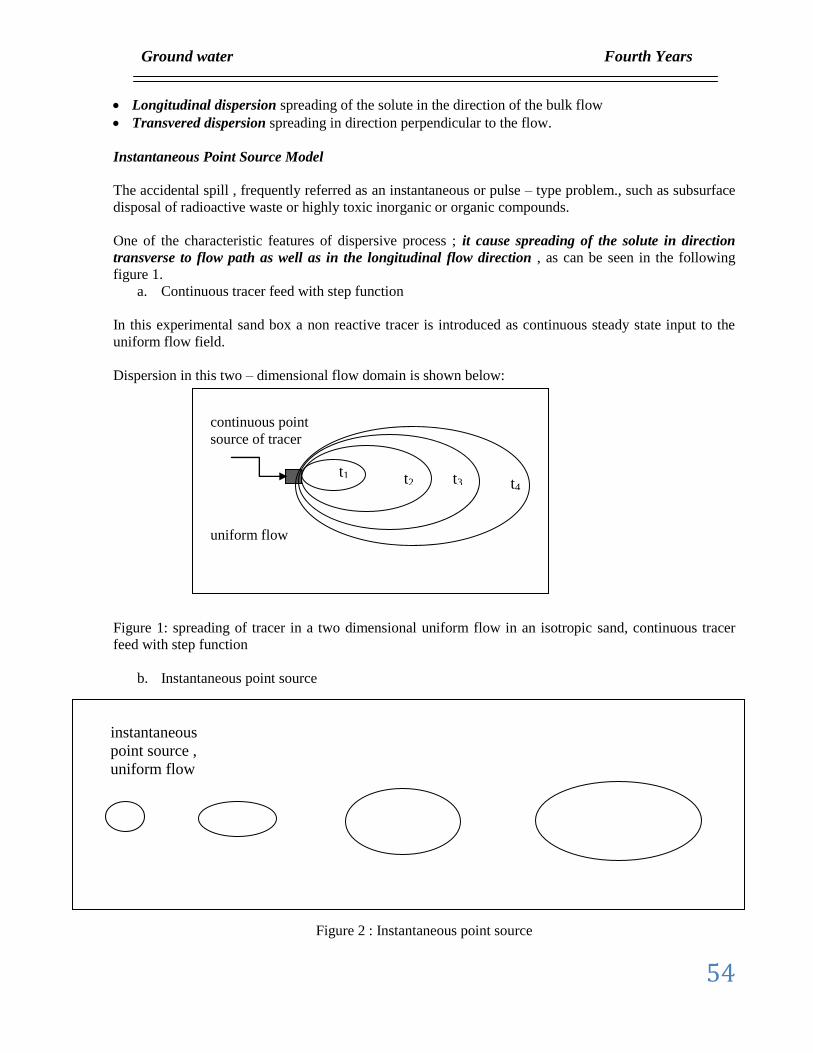
Longitudinal dispersion spreading of the solute in the direction of the bulk flow
Transvered dispersion spreading in direction perpendicular to the flow.
Instantaneous Point Source Model
The accidental spill , frequently referred as an instantaneous or pulse – type problem., such as subsurface
disposal of radioactive waste or highly toxic inorganic or organic compounds.
One of the characteristic features of dispersive process ; it cause spreading of the solute in direction
transverse to flow path as well as in the longitudinal flow direction , as can be seen in the following
figure 1.
a. Continuous tracer feed with step function
In this experimental sand box a non reactive tracer is introduced as continuous steady state input to the
uniform flow field.
Dispersion in this two – dimensional flow domain is shown below:
Figure 1: spreading of tracer in a two dimensional uniform flow in an isotropic sand, continuous tracer
feed with step function
b. Instantaneous point source
Figure 2 : Instantaneous point source
continuous point
source of tracer
t1 t2 t3 t4
uniform flow
instantaneous
point source ,
uniform flow
Ground water Fourth Years
55
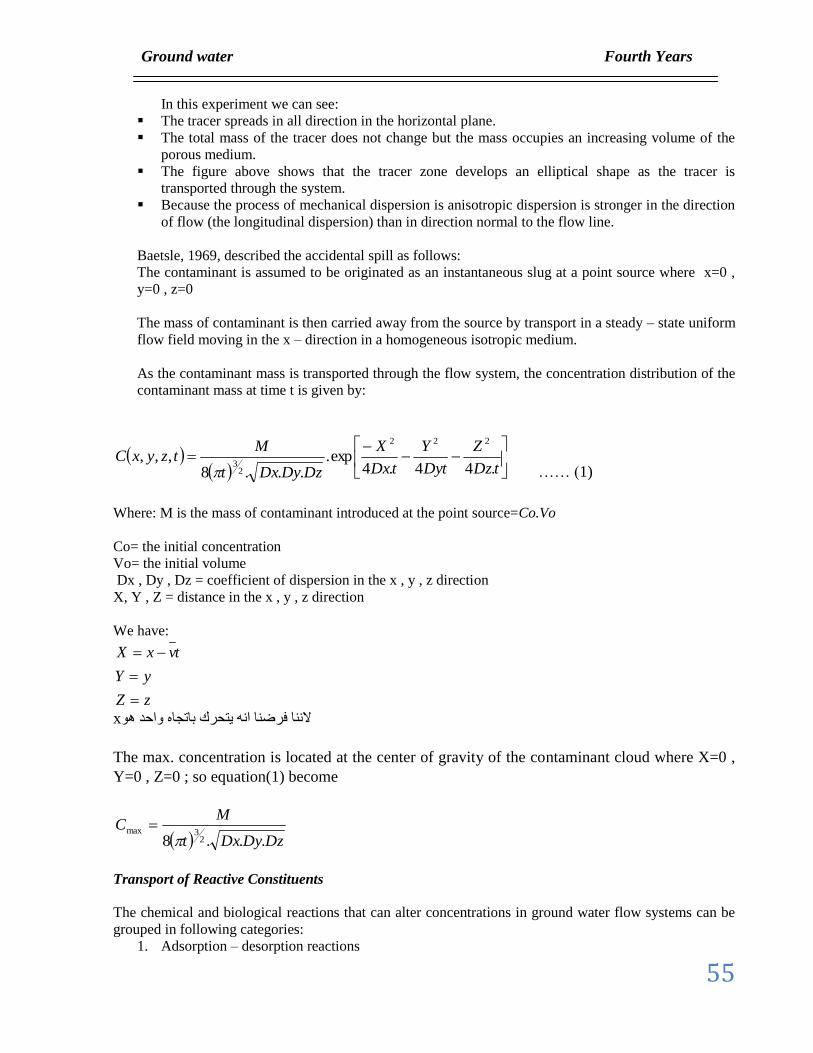
In this experiment we can see:
The tracer spreads in all direction in the horizontal plane.
The total mass of the tracer does not change but the mass occupies an increasing volume of the
porous medium.
The figure above shows that the tracer zone develops an elliptical shape as the tracer is
transported through the system.
Because the process of mechanical dispersion is anisotropic dispersion is stronger in the direction
of flow (the longitudinal dispersion) than in direction normal to the flow line.
Baetsle, 1969, described the accidental spill as follows:
The contaminant is assumed to be originated as an instantaneous slug at a point source where x=0 ,
y=0 , z=0
The mass of contaminant is then carried away from the source by transport in a steady – state uniform
flow field moving in the x – direction in a homogeneous isotropic medium.
As the contaminant mass is transported through the flow system, the concentration distribution of the
contaminant mass at time t is given by:
tDz
Z
Dyt
Y
tDx
X
DzDyDxt
MtzyxC
.44.4exp.
...8,,,
222
23
…… (1)
Where: M is the mass of contaminant introduced at the point source=Co.Vo
Co= the initial concentration
Vo= the initial volume
Dx , Dy , Dz = coefficient of dispersion in the x , y , z direction
X, Y , Z = distance in the x , y , z direction
We have:
zZ
yY
tvxX
x هو الننا فرضنا انه يتحرك باتجاه واحد
The max. concentration is located at the center of gravity of the contaminant cloud where X=0 ,
Y=0 , Z=0 ; so equation(1) become
DzDyDxt
MC
...8 23max
Transport of Reactive Constituents
The chemical and biological reactions that can alter concentrations in ground water flow systems can be
grouped in following categories:
1. Adsorption – desorption reactions
Ground water Fourth Years
56
2. Ion pairing complexation
3. Acid – base reactions
4. Solution- precipitation reactions
5. Oxidation – reduction reactions
6. Microbial cell synthesis
7. Radioactive decay
(We will focus on adsorption here)
For homogeneous saturated media with steady – state flow, the one dimensional form of the advection –
dispersion eq. which include the adsorption process:
t
C
t
S
nx
Cv
x
CD b
2
2
….(1)
Where:
b : Bulk mass density of the porous medium
n : Porosity
S : Mass of the chemical constituent adsorbed on the solid part of the porous medium / unit mass of
solids (mg/kg)
t
S
: The rate at which the constituent is adsorbed (rate of adsorption)
t
S
n
b
; The change in concentration in the fluid causes by adsorption or desorption
Adsorption reactions for contaminants in ground water are normally being very rapid relative to
the flow velocity
The amount of the contaminant that is absorbed by the solids is a function of the concentration in
the solution
)(CfS
And fallowst
C
C
S
t
S
. ……..(2)
And multiply by n
b
t
C
C
S
nt
S
n
bb
.
In which t
S
: partitioning of the contaminant between the solution and the solute = dk (distribution
coefficient)
Ground water Fourth Years
57
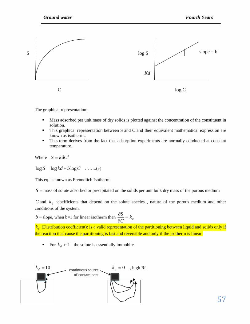
The graphical representation:
Mass adsorbed per unit mass of dry solids is plotted against the concentration of the constituent in
solution.
This graphical representation between S and C and their equivalent mathematical expression are
known as isotherms.
This term derives from the fact that adsorption experiments are normally conducted at constant
temperature.
Where bkdCS
CbkdS logloglog ……..(3)
This eq. is known as Frenndlich Isotherm
S mass of solute adsorbed or precipitated on the solids per unit bulk dry mass of the porous medium
C and dk :coefficients that depend on the solute species , nature of the porous medium and other
conditions of the system.
b slope, when b=1 for linear isotherm then dkC
S
dk (Distribution coefficient): is a valid representation of the partitioning between liquid and solids only if
the reaction that cause the partitioning is fast and reversible and only if the isotherm is linear.
For 1dk the solute is essentially immobile
10dk 0dk , high Rf
S
C
log S
log C
Kd
slope = b
continuous source
of contaminant

Ground water Fourth Years
58
Starting from classical column experiment with two tracers
For general case 0 zyzxyzyxxzxy kkkkkk
The tracers distribution in the column represented schematically.
Advanced of adsorbed and non adsorbed solute
The non reactive tracer move ahead of the reactive tracer speed as a result of dispersion
The reactive tracer spread out but travels behind the non reactive tracer , therefore the adsorbed
tracer is said to be retarded
Move with the
water
The other undergoes to
adsorption
One is not adsorbed
travels through the column
, part of its mass is taken
up by the porous medium
1
C/Co 0.5
0 a b
X
kdn
tx
b
a
v
1
.
tx vb .
Non retarded
retarded tx vb .
Ground water Fourth Years
59
kdnv
vR b
c
f .1
….(4) (retardation equation)
Where fR : retardation factor
v = average linear velocity of ground water
cv = the velocity of the C/Co point on the concentration profile of the retarded constituent
fR can be written as : kdn
nR sf .
11
The velocity of the contaminant becomes less than the velocity of ground water.
kdn
n
v
R
vv
sf
c
..1
1
s =2.65 gm/cm3
kd in ml/gm
the retardation equation predicts the position of the front of a plume to advection transport with
adsorption described by a simple linear isotherm
cv
v : describes how many times faster the ground water ( or non sorbing tracer) is moving relative to the
contaminant being adsorbed.
If kd=0 then no adsorption
The covering equation for mass transport through ground water can be represented as (including
retardation).
t
C
x
C
R
v
x
C
R
Dx
f
x
f
..
2
2
Solution of this equation with the same boundary condition used with Ogata – Bank (1961) eq. is
5.0
...2
...
2
1
f
f
Rtv
tvxRerfc
Co
C
Ground water Fourth Years
60
Radioactive Decay , Biodegradation and Hydrolysis
Consider mass transport involving a first order kinetic reaction
t
CC
x
Cv
x
CD xx
..
2
2
Where : the decay constant for radioactive decay and it equal to 2
1
693.0
t
21
t ; Half life time
The same initial and boundary conditions of the Ogata – Bank equation in one dimension is
5.0
5.0
5.0
..2
41..
.4
112
exp.2
1
tv
vtvx
erfcv
x
Co
C
x
x
x
x
…(1)
Where v is the contaminate velocity and its equal vw/Rf
That is mean the important of retardation in problems of decay or degradation
If =0 eq. (1) reduced to Ogata – Bank eq.
If are large → exp term reach zero → concentration approach zero → the materials decaying faster
than it can be transported through the system
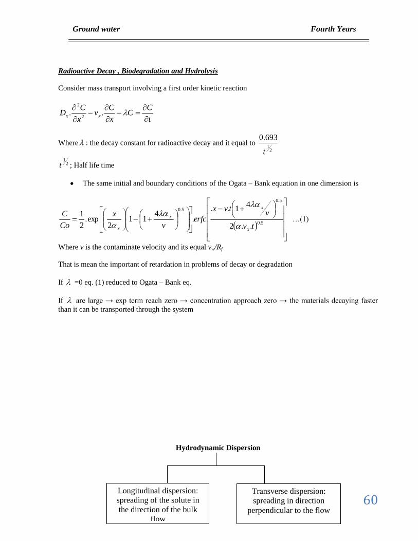
Hydrodynamic Dispersion
Longitudinal dispersion:
spreading of the solute in
the direction of the bulk
flow
Transverse dispersion:
spreading in direction
perpendicular to the flow
Ground water Fourth Years
61
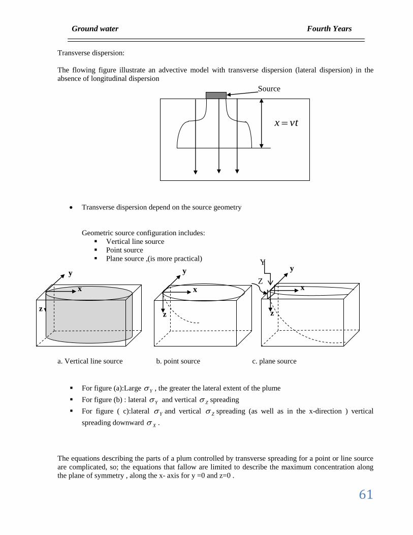
Transverse dispersion:
The flowing figure illustrate an advective model with transverse dispersion (lateral dispersion) in the
absence of longitudinal dispersion
Transverse dispersion depend on the source geometry
Geometric source configuration includes:
Vertical line source
Point source
Plane source ,(is more practical)
a. Vertical line source b. point source c. plane source
For figure (a):Large Y , the greater the lateral extent of the plume
For figure (b) : lateral Y and vertical Z spreading
For figure ( c):lateral Y and vertical Z spreading (as well as in the x-direction ) vertical
spreading downward X .
The equations describing the parts of a plum controlled by transverse spreading for a point or line source
are complicated, so; the equations that fallow are limited to describe the maximum concentration along
the plane of symmetry , along the x- axis for y =0 and z=0 .
Source
vtx
z
y
x
y
z
x
Y
Z
y
z
x
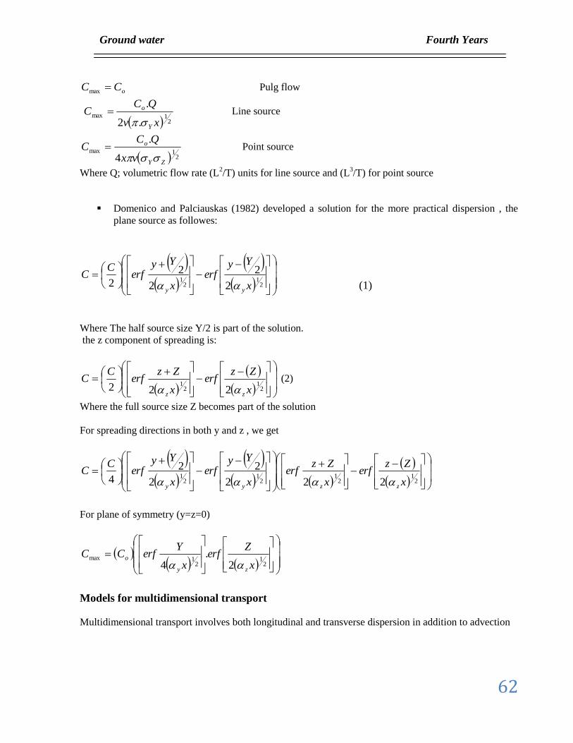
Ground water Fourth Years
62
oCC max
Pulg flow
2
1max
.2
.
xv
QCC
Y
o
Line source
21max
4
.
ZY
o
vx
QCC
Point source
Where Q; volumetric flow rate (L2/T) units for line source and (L
3/T) for point source
Domenico and Palciauskas (1982) developed a solution for the more practical dispersion , the
plane source as followes:
21
21
2
2
2
2
2 x
Yyerf
x
Yyerf
CC
yy (1)
Where The half source size Y/2 is part of the solution.
the z component of spreading is:
21
21
222 x
Zzerf
x
Zzerf
CC
zz (2)
Where the full source size Z becomes part of the solution
For spreading directions in both y and z , we get
21
21
21
21
222
2
2
2
4 x
Zzerf
x
Zzerf
x
Yyerf
x
Yyerf
CC
zzyy
For plane of symmetry (y=z=0)
21
21max
2.
4 x
Zerf
x
YerfCC
zy
o
Models for multidimensional transport
Multidimensional transport involves both longitudinal and transverse dispersion in addition to advection
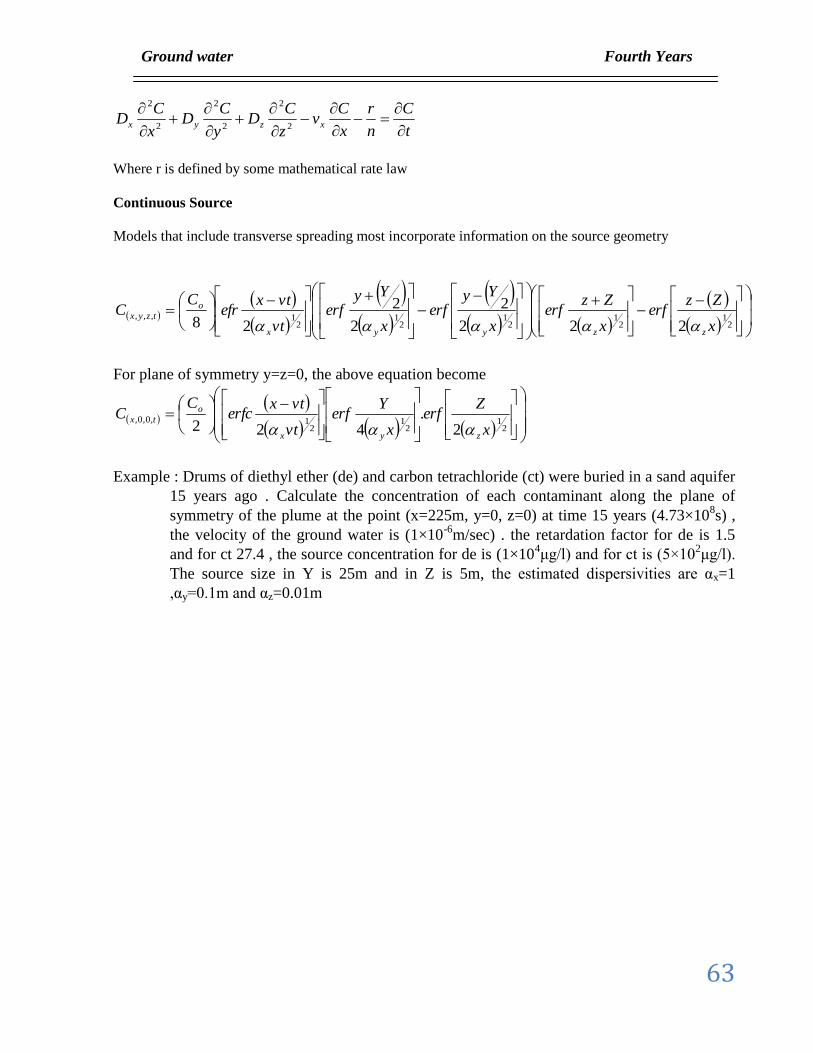
Ground water Fourth Years
63
t
C
n
r
x
Cv
z
CD
y
CD
x
CD xzyx
2
2
2
2
2
2
Where r is defined by some mathematical rate law
Continuous Source
Models that include transverse spreading most incorporate information on the source geometry
21
21
21
21
21,,,
222
2
2
2
28 x
Zzerf
x
Zzerf
x
Yyerf
x
Yyerf
vt
vtxefr
CC
zzyyx
o
tzyx
For plane of symmetry y=z=0, the above equation become
21
21
21,0,0,
2.
422 x
Zerf
x
Yerf
vt
vtxerfc
CC
zyx
o
tx
Example : Drums of diethyl ether (de) and carbon tetrachloride (ct) were buried in a sand aquifer
15 years ago . Calculate the concentration of each contaminant along the plane of
symmetry of the plume at the point (x=225m, y=0, z=0) at time 15 years (4.73×10⁸s) ,
the velocity of the ground water is (1×10⁻⁶
m/sec) . the retardation factor for de is 1.5
and for ct 27.4 , the source concentration for de is (1×10⁴μg/l) and for ct is (5×10
2μg/l).
The source size in Y is 25m and in Z is 5m, the estimated dispersivities are αx=1
,αy=0.1m and αz=0.01m
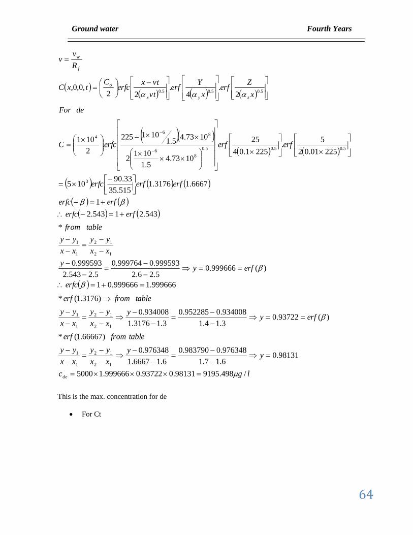
Ground water Fourth Years
64
lgc
yy
xx
yy
xx
yy
tablefromerf
erfyy
xx
yy
xx
yy
tablefromerf
erfc
erfyy
xx
yy
xx
yy
tablefrom
erferfc
erferfc
erferferfc
erferferfcC
deFor
x
Zerf
x
Yerf
vt
vtxerfc
CtxC
R
vv
de
zyx
o
f
w
/498.919598131.093722.0999666.15000
98131.06.17.1
976348.0983790.0
6.16667.1
976348.0
)66667.1(*
)(93722.03.14.1
934008.0952285.0
3.13176.1
934008.0
)3176.1(*
999666.1999666.01
)(999666.05.26.2
999593.0999764.0
5.2543.2
999593.0
*
543.21543.2
1
6667.13176.1515.35
33.90105
22501.02
5.
2251.04
25
1073.45.1
1012
1073.45.1
101225.
2
101
2.
4.
22,0,0,
12
12
1
1
12
12
1
1
12
12
1
1
3
5.05.05.0
86
86
4
5.05.05.0
This is the max. concentration for de
For Ct
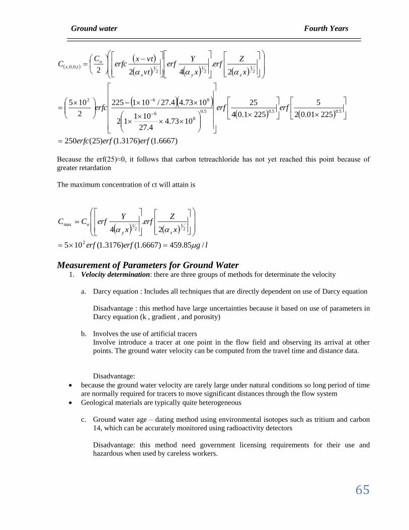
Ground water Fourth Years
65
)6667.1()3176.1()25(250
22501.02
5
2251.04
25
1073.44.27
10112
1073.44.27/101225
2
105
2.
422
5.05.05.0
86
862
21
21
21,0,0,
erferferfc
erferferfc
x
Zerf
x
Yerf
vt
vtxerfc
CC
zyx
o
tx
Because the erf(25)≈0, it follows that carbon tetreachloride has not yet reached this point because of
greater retardation
The maximum concentration of ct will attain is
lgerferf
x
Zerf
x
YerfCC
zy
o
/85.459)6667.1()3176.1(105
2.
4
2
21
21max
Measurement of Parameters for Ground Water 1. Velocity determination: there are three groups of methods for determinate the velocity
a. Darcy equation : Includes all techniques that are directly dependent on use of Darcy equation
Disadvantage : this method have large uncertainties because it based on use of parameters in
Darcy equation (k , gradient , and porosity)
b. Involves the use of artificial tracers
Involve introduce a tracer at one point in the flow field and observing its arrival at other
points. The ground water velocity can be computed from the travel time and distance data.
Disadvantage:
because the ground water velocity are rarely large under natural conditions so long period of time
are normally required for tracers to move significant distances through the flow system
Geological materials are typically quite heterogeneous
c. Ground water age – dating method using environmental isotopes such as tritium and carbon
14, which can be accurately monitored using radioactivity detectors
Disadvantage: this method need government licensing requirements for their use and
hazardous when used by careless workers.
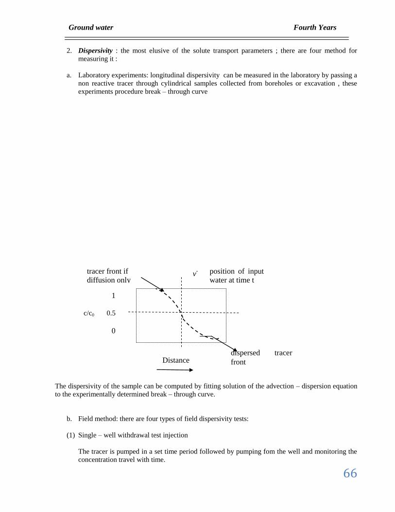
Ground water Fourth Years
66
2. Dispersivity : the most elusive of the solute transport parameters ; there are four method for
measuring it :
a. Laboratory experiments: longitudinal dispersivity can be measured in the laboratory by passing a
non reactive tracer through cylindrical samples collected from boreholes or excavation , these
experiments procedure break – through curve
The dispersivity of the sample can be computed by fitting solution of the advection – dispersion equation
to the experimentally determined break – through curve.
b. Field method: there are four types of field dispersivity tests:
(1) Single – well withdrawal test injection
The tracer is pumped in a set time period followed by pumping fom the well and monitoring the
concentration travel with time.
1
c/c0 0.5
0
Distance
v-
dispersed tracer
front
position of input
water at time t
tracer front if
diffusion only
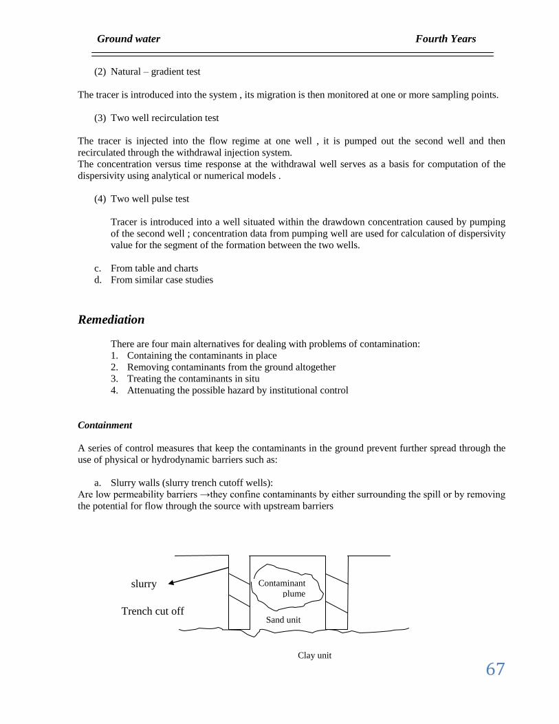
Ground water Fourth Years
67
(2) Natural – gradient test
The tracer is introduced into the system , its migration is then monitored at one or more sampling points.
(3) Two well recirculation test
The tracer is injected into the flow regime at one well , it is pumped out the second well and then
recirculated through the withdrawal injection system.
The concentration versus time response at the withdrawal well serves as a basis for computation of the
dispersivity using analytical or numerical models .
(4) Two well pulse test
Tracer is introduced into a well situated within the drawdown concentration caused by pumping
of the second well ; concentration data from pumping well are used for calculation of dispersivity
value for the segment of the formation between the two wells.
c. From table and charts
d. From similar case studies
Remediation
There are four main alternatives for dealing with problems of contamination:
1. Containing the contaminants in place
2. Removing contaminants from the ground altogether
3. Treating the contaminants in situ
4. Attenuating the possible hazard by institutional control
Containment
A series of control measures that keep the contaminants in the ground prevent further spread through the
use of physical or hydrodynamic barriers such as:
a. Slurry walls (slurry trench cutoff wells):
Are low permeability barriers →they confine contaminants by either surrounding the spill or by removing
the potential for flow through the source with upstream barriers
Contaminant
plume
Sand unit
Clay unit
slurry
Trench cut off
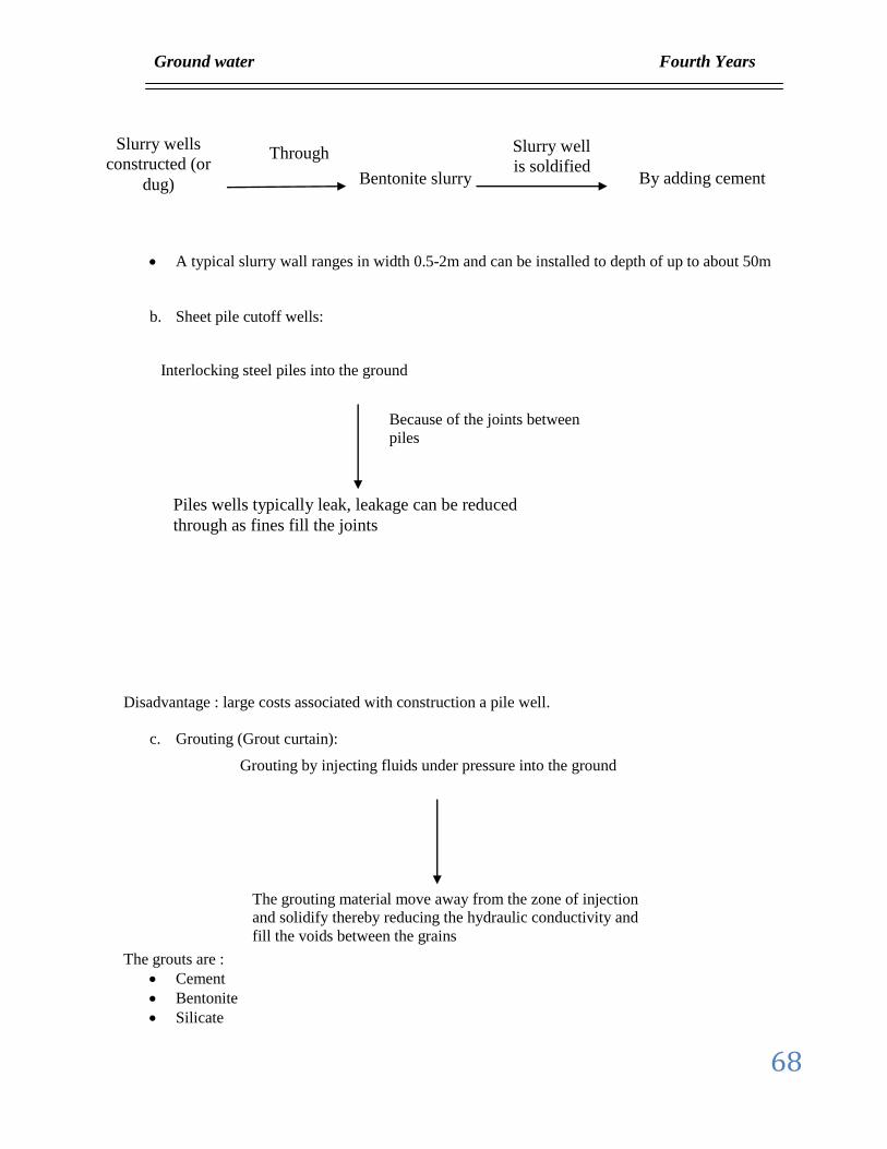
Ground water Fourth Years
68
A typical slurry wall ranges in width 0.5-2m and can be installed to depth of up to about 50m
b. Sheet pile cutoff wells:
Disadvantage : large costs associated with construction a pile well.
c. Grouting (Grout curtain):
The grouts are :
Cement
Bentonite
Silicate
Slurry wells
constructed (or
dug)
Through
Bentonite slurry
Slurry well
is soldified By adding cement
Grouting by injecting fluids under pressure into the ground
The grouting material move away from the zone of injection
and solidify thereby reducing the hydraulic conductivity and
fill the voids between the grains
Interlocking steel piles into the ground
Piles wells typically leak, leakage can be reduced
through as fines fill the joints
Because of the joints between
piles
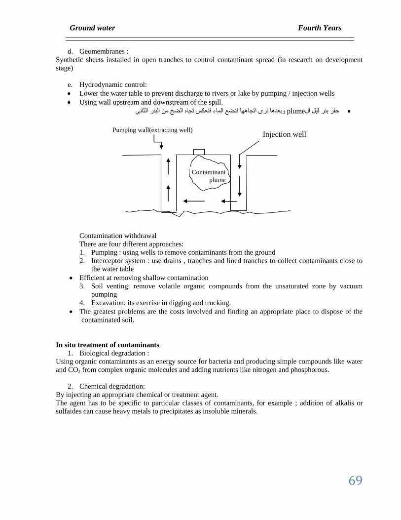
Ground water Fourth Years
69
d. Geomembranes :
Synthetic sheets installed in open tranches to control contaminant spread (in research on development
stage)
e. Hydrodynamic control:
Lower the water table to prevent discharge to rivers or lake by pumping / injection wells
Using wall upstream and downstream of the spill.
حفر بئر قبل الplume وبعدها نرى اتجاهها فنضع الماء فنعكس تجاه الضخ من البئر الثاني
Contamination withdrawal
There are four different approaches:
1. Pumping : using wells to remove contaminants from the ground
2. Interceptor system : use drains , tranches and lined tranches to collect contaminants close to
the water table
Efficient at removing shallow contamination
3. Soil venting: remove volatile organic compounds from the unsaturated zone by vacuum
pumping
4. Excavation: its exercise in digging and trucking.
The greatest problems are the costs involved and finding an appropriate place to dispose of the
contaminated soil.
In situ treatment of contaminants
1. Biological degradation :
Using organic contaminants as an energy source for bacteria and producing simple compounds like water
and CO2 from complex organic molecules and adding nutrients like nitrogen and phosphorous.
2. Chemical degradation:
By injecting an appropriate chemical or treatment agent.
The agent has to be specific to particular classes of contaminants, for example ; addition of alkalis or
sulfaides can cause heavy metals to precipitates as insoluble minerals.
Contaminant
plume
Pumping wall(extracting well) Injection well
Ground water Fourth Years
70
Steps for dealing with problems of contaminants in ground water
Starting with field slurry
Site characteristics
a. Aquifer properties
1. Permeability
2. Specific yield
3. Clay content of soil
4. Heterogeneity of formation
5. Depth
6. Thickness
7. Direction of ground water
8. Reachrge and discharge
9. Seasonal fluctuation in water table
b. Ground water quality
1. Inorganic nutrient levels
2. Precipitation of inorganic nutrients
3. Dissolved oxygen content
c. Contaminant characteristics
1. Type
2. Concentration
3. Areal and vertical extent of contamination
4. Location of released material in aquifer (dissolved , floating , trapped , or sinking)
5. Heterogeneity of contamination
6. Biodegradability of contaminants
7. Presence and quantity of toxic agent
8. Nature of release –acute , chronic or periodic
9. Time since release
10. Effect of physical weathering or a biotic reaction on contaminants
d. Microbial characteristics
1. Presence of active microbial population
2. Acclimation to contaminant
3. Nutrient requirements for optimal growth
4. Extent of biodegradation that can be achieved
5. Rating biodegradation
Related Documents