Grid cell symmetry is shaped by environmental geometry

LETTERdoi:10.1038/nature14153

Grid cell symmetry is shaped by environmentalgeometryJulija Krupic1*, Marius Bauza1*, Stephen Burton1, Caswell Barry1 & John O’Keefe1,2

Grid cells represent an animal’s location by firing in multiple fieldsarranged in a striking hexagonal array1. Such an impressive and con-stant regularity prompted suggestions that grid cells represent auniversal and environmental-invariant metric for navigation1,2. Orig-inally the properties of grid patterns were believed to be independ-ent of the shape of the environment and this notion has dominatedalmost all theoretical grid cell models3–6. However, several studiesindicate that environmental boundaries influence grid firing7–10,though the strength, nature and longevity of this effect is unclear. Herewe show that grid orientation, scale, symmetry and homogeneity arestrongly and permanently affected by environmental geometry. Wefound that grid patterns orient to the walls of polarized enclosuressuch as squares, but not circles. Furthermore, the hexagonal grid sym-metry is permanently broken in highly polarized environments suchas trapezoids, the pattern being more elliptical and less homogen-eous. Our results provide compelling evidence for the idea that en-vironmental boundaries compete with the internal organization ofthe grid cell system to drive grid firing. Notably, grid cell activity ismore local than previously thought and as a consequence cannotprovide a universal spatial metric in all environments.

Navigation is performed on the basis of information about self-motionand external cues, including enclosure geometry, the latter dominatingnon-geometric information such as visual landmarks, textures andsmells11–13. In mammals the hippocampal formation is required for spa-tial navigation14 and its neurons encode the animal’s position (place cells15

and grid cells1), head direction (head direction cells16) and proximityto boundaries (boundary cells17,18). The spatial activity of boundary andplace cells is known to be affected by environmental geometry17–19. Gridcells may also be influenced by changes to boundaries, in particularreflecting distortions of a familiar enclosure by rescaling in the samedirection7. These changes ameliorate with time and cells tend to returntowards their canonical patterns, reinforcing the idea that internal pro-cesses at the individual cell or network level predominantly determine

the grid pattern2. Here we demonstrate that environmental geometryexerts an important and permanent influence on grid cell firing. Undercertain circumstances, it can overcome internal network processes andlead to profound distortions of the grid pattern.

In geometrically symmetrical enclosures such as circles, distal cuescontrol the orientation of grid patterns which follow cue rotation1. Incontrast, we found that in geometrically polarized enclosures, such assquares, greater control is exercised by the arena. A 45u rotation of thearena commensurately rotates the grid pattern despite prominent dis-tal cues remaining stationary (Fig. 1a, b, mean grid rotation6 42.5u6 2.9u(mean 1 s.e.m., here and elsewhere), n 5 5 rats/5 modules, 19 grid cells,not different from 45u, P 5 0.44, t 5 20.85, n 5 5, df 5 4, one-samplet-test). Notably, no changes were observed for 90u rotations for whichgeometry remains unchanged but local cues such as smells and tex-tures move (mean grid orientation 1.1u6 0.9u not different from 0u,P 5 0.29, t 5 1.21, n 5 5, df 5 4, one-sample t-test).

We explored which aspects of the grid pattern were affected by en-vironmental geometry, beginning with the influence of the enclosurewalls over grid orientation. A total of 275 grid cells (62 modules, 41 rats)were recorded while animals foraged in square enclosures (Fig. 1c andExtended Data Figs 1 and 2). Across rats, the orientation of the gridsaligned at a mean angle of 8.8u6 0.6u to the enclosure walls (Fig. 1d, e;P 5 0.015, Z 5 4.2, Rayleigh test for non-uniformity; P 5 0.04 versusshuffled data, see Extended Data Fig. 3). In unpolarized circular envi-ronments grid orientations were less clustered than in the square(Fig. 1f; P 5 0.025, t 5 2.4, df 5 21; two-sample t-test). Clusteringdid not arise from behavioural biases: the distribution of velocitiesand directional headings were not different between squares and circles(P 5 0.34, t 5 0.98, df 5 21 for headings; P 5 0.89, t 5 0.15, df 5 21for velocity; two-sample t-test; Extended Data Fig. 4) suggesting thatgrid patterns align to the walls in polarized enclosures due to the directinfluence of environmental geometry and not through changes inbehaviour.

*These authors contributed equally to this work.

1Department of Cell and Developmental Biology, University College London, London WC1E 6BT, UK. 2Sainsbury Wellcome Centre, University College London, London WC1E 6BT, UK.

0.5 m

c

ed f60º

240º

120º

300º

180º 0º

Orientation (deg)

60º

240º

120º

300º

180º 0º

Orientation (deg)

ba

C1C1C2C2C3C3

Square Circle

Ch

an

ge in

o

rien

tatio

n (d

eg

)

45 degrotation

90 degrotation

0

20

40

0.80.8

0.40.4

0.80.8

0.40.4

Nu

mb

er

of

co

mp

on

en

ts

Orientation (deg)

0 100 200 3000

5

10

Orientation relative

to wall (deg)

Nu

mb

er

of

co

mp

on

en

ts

0 8 160

5

10

15

Figure 1 | Grid orientation aligns to walls insquares. a, b, 45u rotation of a square (middle)rotates the grid pattern by the same amount(2 typical grid cells from 2 rats, distal cue card inorange, P 5 0.44, t 5 20.85, n 5 5, df 5 4, one-sample t-test, mean 1 s.e.m.). c, Three typicalgrid cell rate maps (top) and their spatialautocorrelograms (bottom) (n 5 3 rats).Orientations of the three main grid componentsin black, vertical and horizontal walls in red dashedlines. d, Distribution of grid orientations for 62 gridmodules (41 rats) in squares, e is clustered at8.8u6 0.6u (mean 1 s.e.m.) from the vertical orhorizontal walls (P 5 0.015, Z 5 4.2, Rayleigh test),and f is significantly more clustered in square(12 modules) than circle (11 modules) in the same7 rats (P 5 0.025, t 5 2.4, df 5 21; two-samplet-test).

2 3 2 | N A T U R E | V O L 5 1 8 | 1 2 F E B R U A R Y 2 0 1 5

Macmillan Publishers Limited. All rights reserved©2015

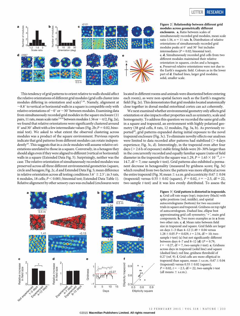
This tendency of grid patterns to orient relative to walls should affectthe relative orientations of different grid modules (grid cells cluster intomodules differing in orientation and scale)7,10. Namely, alignment at,8.8u to vertical or horizontal walls in a square is compatible only withrelative orientations of ,0uor ,30ubetween modules. Examining datafrom simultaneously recorded grid modules in the square enclosure (11pairs, 11 rats, mean scale ratio7,8,10 between modules 1.56 or ,p/2, Fig. 2a),we found that relative orientations were significantly clustered around0u and 30u albeit with a few intermediate values (Fig. 2b; P 5 0.02, bino-mial test). We asked to what extent the observed clustering acrossmodules was a product of the square environment. Previous reportsindicate that grid patterns from different modules can rotate indepen-dently10. This suggests that in a circle modules will assume relative ori-entations unrelated to those in a square. Conversely, in a hexagon theyshould align even if they were aligned to different (vertical or horizontal)walls in a square (Extended Data Fig. 5). Surprisingly, neither was thecase. The relative orientation of simultaneously recorded modules waspreserved across all three different environmental geometries (square,circle and hexagon; Fig. 2c, d and Extended Data Fig. 5; mean differencein relative orientation across all testing conditions 3.6u6 2.5u; in 3 rats,6 modules, 18 cells; P , 0.001; binomial test; Extended Data Table 1).Relative alignment by other sensory cues was excluded (enclosures were

located in different rooms and animals were disoriented before enteringeach room), as were non-spatial factors such as the Earth’s magneticfield (Fig. 2e). This demonstrates that grid modules located anatomicallyclose together in dorsal medial entorhinal cortex can act coherently.

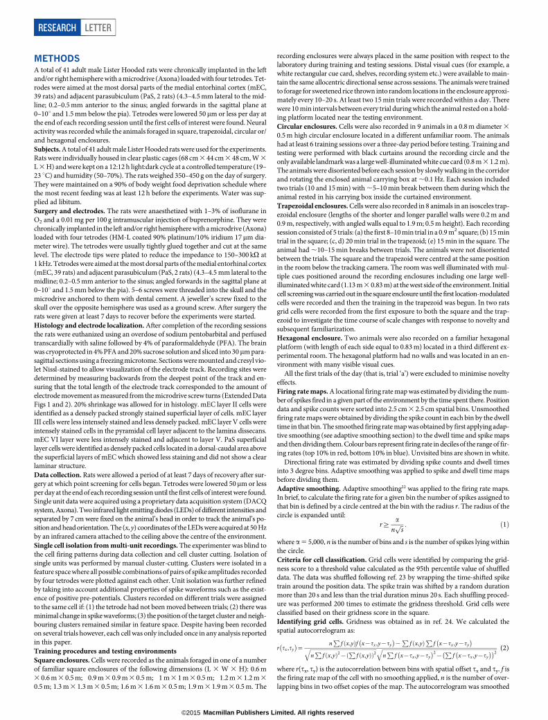
We next examined whether environmental geometry only affects gridorientation or also impacts other properties such as symmetry, scale andhomogeneity. To address this question we recorded the same grid cellsin a square and trapezoid, an environment with highly polarized geo-metry (38 grid cells, 8 rats, 12 modules, Fig. 3a, b). As previously re-ported20, grid patterns expanded during initial exposure to the noveltrapezoid enclosure (Fig. 3c). To eliminate novelty effects our analyseswere limited to data recorded after patterns had stabilized (. 4 daysexperience; Fig. 3c, d). Interestingly, in the trapezoid even after fourdays (. 2.6 h of exposure) stable firing fields were 20–30% larger thanin the concurrently recorded and equally familiar square (ratio of fielddiameter in the trapezoid to the square was 1.29, P 5 1.65 3 1026, t 5

14.7, df 5 7; one-sample t-test). Grid patterns also exhibited a perma-nent decrease in hexagonality (measured by gridness score; Fig. 3e)which resulted from two factors: the pattern was more elliptical acrossthe entire trapezoid (Fig. 3f; mean 6 s.e.m. grid eccentricity: 0.67 6 0.04(trapezoid) versus 0.55 6 0.02 (square), P 5 0.02, t 5 22.5, df 5 22,two-sample t-test) and it was less evenly distributed. To assess the

e

b

d

0.5 m

r2067

a cr2121

Scale ratio

Num

ber

of

mo

dule

s

1.2 1.6 20

2

4

6

Orientation (deg)N

um

ber

of

mo

dule

s

0 10 20 300

2

4

6

N

Figure 2 | Relationship between different gridmodules across geometrically differentenclosures. a, Ratio between scales ofsimultaneously recorded grid modules, mean scaleratio 1.56, n 5 11 rats. b, Distribution of relativeorientations of simultaneously recorded gridmodules peaks at 0u and 30u but includesintermediates (P 5 0.02; binomial test).c, d, Simultaneously recorded grid cells from twodifferent modules maintained their relativeorientation in squares, circles and a hexagon.e, Preserved relative orientations were not due tothe Earth’s magnetic field. Colours as in the lowerpart of d. Dashed lines, larger grid modules;solid, smaller scale.

0.5 m

a

+

++ +

+

+

+

++

+++

b

c d

17.3 Hz15.5 Hz

–0.131.41

0.3

0.6

0.3 0.9

Ellipticity square

0.9

0.6

Elli

pticity t

rap

ezo

id

0.5 m

f

–0.951.04

1.38 0.25

0

1

2

Exper

ienc

ed

4–7

days

Exper

ienc

ed

8–12

day

s

Not

exp

erienc

ed

1–3

days

Exper

ienc

ed

4–12

day

s0

1

2

Rela

tive incre

ase *

e

Days

Grid

ness

0 5 10 15–1

0

1

0.27

in fi

eld

siz

e

Rela

tive incre

ase

in fi

eld

siz

e

Figure 3 | Grid pattern is distorted in trapezoids.a, Grid cell rate maps (top), trajectory (black) withspike positions (red, middle), and spatialautocorrelograms (bottom) for two successivetrials in square and trapezoid. Gridness on top rightof autocorrelogram. Dashed line, ellipse bestapproximating grid cell symmetry; ‘1’, main gridcomponents. b, Two more examples as in a fromtwo other rats. c, d, Mean ratio between fieldsize in trapezoid and square. Grid fields are largeron days 1–3 than 4–12 (1.49 1 0.04 versus1.28 6 0.05 P 5 0.029, t 5 2.54, df 5 10; two-sample t-test) (c) but not significantly differentbetween days 4–7 and 8–12 (d) (P 5 0.79,t 5 20.27, df 5 7, two-sample t-test). e, Gridnessacross days in trapezoid (solid line) and square(dashed line); red line, gridness threshold of0.27 (ref. 9). f, Grid cells are more elliptical intrapezoid than square, mean 6 s.e.m.: 0.67 6 0.04(trapezoid) versus 0.55 6 0.02 (square),P 5 0.02, t 5 22.5, df 5 22, two-sample t-test(all means 6 s.e.m.).

LETTER RESEARCH

1 2 F E B R U A R Y 2 0 1 5 | V O L 5 1 8 | N A T U R E | 2 3 3

Macmillan Publishers Limited. All rights reserved©2015

latter, we divided the trapezoid and square into two equal parts (Fig. 4a;area of half-trapezoid 0.51 m2, half-square 0.41 m2) and compared firingon either side. Figure 4b, c shows that the local spatial structure (definedby the spatial autocorrelogram) differs more strongly between the twosides of the trapezoid than between the sides of the square (r 5 0.11 6

0.07 versus 0.50 6 0.06, trapezoid and square, respectively, P , 0.001,t 5 24.0, df 5 18, two-sample t-test, 10 grid modules, 32 grid cells).Moreover, gridness was lower in the left of the trapezoid than the right(Fig. 4d, 20.35 6 0.07 and 0.23 6 0.17, respectively, P 5 0.006, t 5

23.11, df 5 18, two-sample t-test) but not in the square (0.71 6 0.09and 0.68 6 0.11, P 5 0.87, t 5 0.17, df 5 18, two-sample t-test). Grid-ness was lower on the right of the trapezoid compared to both parts ofthe square even though they are of comparable shape and area (P 5

0.009; F 5 6.18; two-way ANOVA), suggesting an influence from theleft side of the trapezoid. Additionally, the diameters of the individualfields were larger on the left of the trapezoid than the right (Fig. 4e,P , 0.001, t 5 4.1, df 5 18, two-sample t-test) but not in the square(P 5 0.39, t 5 0.88, df 5 18, two-sample t-test). Notably, the field sizeson the right of the trapezoid were not different from those on either sideof the square (P 5 0.15; F 5 2.07; two-way ANOVA).

We also examined how the orientations and wavelengths of the threegrid components computed from the spatial autocorrelogram differedbetween sides of the two environments (Fig. 4f, g). The orientation ofthe first component (closest to the horizontal axis; Extended Data Fig. 6)was no more variable between the sides of the trapezoid than the sidesof the square (mean orientation change of 11.6u6 2.5u and 8.0u6 0.8u,trapezoid and square, respectively, P 5 0.19, t 5 21.36, df 5 16, two-sample t-test). However, the other two components differed more inthe trapezoid than in the square (second: 19.2u6 4.9u and 4.7u6 0.3uP 5 0.004, t 5 23.41, df 5 14; third: 21.4u6 4.6u and 7.9u6 0.8u, P 5

0.005, t 5 -3.3, df 5 14, two-sample t-test). Similarly, the first wavelengthwas no more variable in the trapezoid than the square (mean wavelengthchange: 4.4 6 1.2 versus 2.3 6 0.4 cm, trapezoid and square, respect-ively, P 5 0.12, t 5 21.6, df 5 16, two-sample t-test), while the differ-ences for the second (6.1 6 1.0 versus 1.9 6 0.5 cm, P 5 0.001, t 5 24.1,df 5 14) and third wavelengths (10.1 6 2.8 cm versus 3.8 6 0.7 cm,

P 5 0.02, t 5 22.7, df 5 14) were more pronounced in the trapezoid.These localized changes in grid components manifest as a rotation andstretching of the grid pattern across the trapezoid (Fig. 4h–k). Indeedthe spatial correlation between the two halves of the trapezoid at theoptimal rotation angle (that is, the one maximising the correlation be-tween left and right sides) was still lower compared to the square (Fig. 4h, j;r 5 0.30 6 0.05 trapezoid and 0.63 6 0.05 square, P 5 0.0002, t 5 24.6,df 5 18, two-sample t-test), indicating rescaling as well as rotation(Fig. 4k).

To eliminate the possibility that these observations arose from under-sampling of the grid pattern in the trapezoid, we generated idealizedgrid firing (scale and orientation matched to the data) for a square andtrapezoid environment (Extended Data Fig. 7). This control data exhib-ited neither an increase in ellipticity nor in inhomogeneity. Further-more, although the animals’ behaviour was polarized between the twohalves of the trapezoid (Extended Data Fig. 4), there was no correlationbetween the extent of polarization and differences in grid properties be-tween the sides, ruling out a behavioural explanation. Indeed it is knownthat stereotypical behaviour in the open field does not significantly de-grade the hexagonal grid structure21.

Our results show that most assumptions about the invariant natureof grid cell firing are invalid. In particular the role of environmentalboundaries has been underestimated. Our findings reveal that grid pat-terns are permanently shaped by environmental geometry as well as byinternal network processes (Extended Data Figs 8 and 9). Notably, wehave shown that grid patterns can be inhomogeneous even within a con-tinuous two-dimensional space, due to the influence of non-parallelboundaries (probably signalled by boundary cells). A differential influ-ence from the boundaries probably also accounts for the ellipticity ofdifferent grid modules10, as well as the non-hexagonal symmetry of spa-tially periodic non-grid cells8. The results challenge the idea that the gridcell system can act as a universal spatial metric for the cognitive map asgrid patterns change markedly between enclosures and even within thesame enclosure. An intriguing alternative is that grid cells provide a spa-tial metric but that the asymmetries induced by highly polarized envir-onments such as trapezoids produce distortions in the perception of space.

c

d e f g

h

a

–20 0 20

–0.3

0

0.3

0.6

Rotation (deg)

Co

rrela

tio

n

–20 0 20–0.5

0

0.5

1

Rotation (deg)

Co

rrela

tio

n0.5 m

b

Ch

an

ge in

orien

tatio

n (d

eg

)

0

10

20

30

1 2 30

10

20

1 2 3

Ch

an

ge in

wavele

ng

th (cm

)

i j

k

0.5 m

Sim

ilarity

tr sq0

0.3

0.6–0.47 0.55

0.83 0.75

Left Right

tr

sq

Grid

ness

–0.5

0

0.5

1

Trapezoid

Square

0

10

20

30 Trapezoid

Square

Correlation

0 0.4 0.80

10

20

30

Rotation (deg)

–20 0 200

10

20

30

Mo

du

les (%

)

Left

Right

Left

Rig

htLe

ft

Rig

ht

Fie

ld d

iam

ete

r (c

m)

Left

Rig

htLe

ft

Rig

ht

Mo

du

les (%

)

Figure 4 | Grid pattern is inhomogeneous intrapezoids. a, Grid cell rate maps for the same cellin trapezoid and square. Dashed line dividesenclosures into equal areas. b, c, Autocorrelogramsfor each side of the trapezoid (tr) and square (sq)are significantly more similar in the square thanthe trapezoid (c). d, Gridness on two sides of thetrapezoid and square. Dashed line representsgridness threshold9. e, Field diameter is larger onthe left than the right of the trapezoid (P , 0.001,t 5 4.1, df 5 18, two-sample t-test) but notdifferent in the square (P 5 0.39, t 5 0.88, df 5 18,two-sample t-test). f, g, Change in orientations (f)and wavelengths (g) of left/right parts oftrapezoid (black) and square (blue). h, j, Rotationof right part of autocorrelogram relative to leftoptimizes correlation in trapezoid but notsquare (h) but still leaves a lower similarity (j)(P 5 0.0002, t 5 24.6, df 5 18, two-sample t-test,32 grid cells, 8 rats, 10 different grid modules).i, Average grid rotation between two sides oftrapezoid (solid line) and square (dashed line).k, Another example of right-to-left grid expansionand rotation in trapezoid. All means 6 s.e.m.,except for f, g, which shows means 6 s.d.

RESEARCH LETTER

2 3 4 | N A T U R E | V O L 5 1 8 | 1 2 F E B R U A R Y 2 0 1 5

Macmillan Publishers Limited. All rights reserved©2015

Online Content Methods, along with any additional Extended Data display itemsandSourceData, are available in the online version of the paper; references uniqueto these sections appear only in the online paper.

Received 11 June; accepted 11 December 2014.

1. Hafting, T., Fyhn, M., Molden, S., Moser, M.-B. & Moser, E. I. Microstructure of aspatial map in the entorhinal cortex. Nature 436, 801–806 (2005).

2. Buzsaki, G. & Moser, E. I. Memory, navigation and theta rhythm in thehippocampal-entorhinal system. Nature Neurosci. 16, 130–138 (2013).

3. Fuhs, M. C. & Touretzky, D. S. A spin glass model of path integration in rat medialentorhinal cortex. J. Neurosci. 26, 4266–4276 (2006).

4. Fiete, I. R., Burak, Y. & Brookings, T. What grid cells convey about rat location.J. Neurosci. 28, 6858–6871 (2008).

5. Burgess, N. Grid cells and theta as oscillatory interference: theory and predictions.Hippocampus 18, 1157–1174 (2008).

6. Hasselmo, M. E. Grid cell mechanisms and function: contributions of entorhinalpersistent spiking and phase resetting. Hippocampus 18, 1213–1229 (2008).

7. Barry, C., Hayman, R., Burgess, N. & Jeffery, K. J. Experience-dependent rescalingof entorhinal grids. Nature Neurosci. 10, 682–684 (2007).

8. Krupic, J., Burgess, N.& O’Keefe, J.Neural representations of locationcomposedofspatially periodic bands. Science 337, 853–857 (2012).

9. Krupic, J., Bauza, M., Burton, S., Lever, C. & O’Keefe, J. How environment geometryaffects grid cell symmetry and what we can learn from it. Philos. Trans. R. Soc. B369, 20130188 (2014).

10. Stensola, H. et al. The entorhinal grid map is discretized. Nature 492, 72–78(2012).

11. Gallistel, C. The Organization of Action: A New Synthesis (Lawrence ErlbaumAssociates, 2013).

12. Cheng, K. A purely geometric module in the rat’s spatial representation. Cognition23, 149–178 (1986).

13. Kelly, J. W., McNamara, T. P., Bodenheimer, B., Carr, T. H. & Rieser, J. J. The shape ofhuman navigation:how environmental geometry isused inmaintenanceof spatialorientation. Cognition 109, 281–286 (2008).

14. Morris, R. G. M., Garrud, P., Rawlins, J. N. P. & O’Keefe, J. Place navigation impairedin rats with hippocampal lesions. Nature 297, 681–683 (1982).

15. O’Keefe, J. & Dostrovsky, J. The hippocampus as a spatial map. Preliminaryevidence from unit activity in the freely-moving rat. Brain Res. 34, 171–175(1971).

16. Taube, J. S., Muller, R. U. & Ranck, J. B., Jr. Head-direction cells recorded from thepostsubiculum in freely moving rats. I. Description and quantitative analysis.J. Neurosci. 10, 420–435 (1990).

17. Solstad, T., Boccara, C. N., Kropff, E., Moser, M.-B. & Moser, E. I. Representationof geometric borders in the entorhinal cortex. Science 322, 1865–1868(2008).

18. Barry, C. et al. The boundary vector cell model of place cell firing and spatialmemory. Rev. Neurosci. 17, 71–97 (2006).

19. O’Keefe, J. & Burgess, N. Geometric determinants of the place fields ofhippocampal neurons. Nature 381, 425–428 (1996).

20. Barry, C., Ginzberg, L. L., O’Keefe, J. & Burgess, N. Grid cell firing patterns signalenvironmental novelty by expansion. Proc. Natl Acad. Sci. USA 109, 17687–17692(2012).

21. Derdikman, D. et al. Fragmentation of grid cell maps in a multicompartmentenvironment. Nature Neurosci. 12, 1325–1332 (2009).

Acknowledgements We thank J. Poort for discussions. The research was supported bygrants from the Wellcome Trust and the Gatsby Charitable Foundation. J.K. is aWellcome Trust Sir Henry Welcome Fellow. C.B. is a Royal Society and Wellcome TrustSir Henry Dale Fellow. This work was conducted in accordance with the UK Animals(Scientific Procedures) Act (1986).

Author Contributions J.K. and M.B. planned experiments and analyses. J.K., S.B. andC.B performed the experiments. J.K. and M.B. analysed the data. J.K., M.B., C.B. andJ.O’K. wrote the manuscript. All authors discussed the results and contributed to themanuscript.

Author Information Reprints and permissions information is available atwww.nature.com/reprints. The authors declare no competing financial interests.Readers are welcome to comment on the online version of the paper. Correspondenceand requests for materials should be addressed to J.K. ([email protected]).

LETTER RESEARCH

1 2 F E B R U A R Y 2 0 1 5 | V O L 5 1 8 | N A T U R E | 2 3 5

Macmillan Publishers Limited. All rights reserved©2015

METHODSA total of 41 adult male Lister Hooded rats were chronically implanted in the leftand/or right hemisphere with a microdrive (Axona) loaded with four tetrodes. Tet-rodes were aimed at the most dorsal parts of the medial entorhinal cortex (mEC,39 rats) and adjacent parasubiculum (PaS, 2 rats) (4.3–4.5 mm lateral to the mid-line; 0.2–0.5 mm anterior to the sinus; angled forwards in the sagittal plane at0–10u and 1.5 mm below the pia). Tetrodes were lowered 50mm or less per day atthe end of each recording session until the first cells of interest were found. Neuralactivity was recorded while the animals foraged in square, trapezoidal, circular or/and hexagonal enclosures.Subjects. A total of 41 adult male Lister Hooded rats were used for the experiments.Rats were individually housed in clear plastic cages (68 cm 3 44 cm 3 48 cm, W 3

L 3 H) and were kept on a 12:12 h light:dark cycle at a controlled temperature (19–23 uC) and humidity (50–70%). The rats weighed 350–450 g on the day of surgery.They were maintained on a 90% of body weight food deprivation schedule wherethe most recent feeding was at least 12 h before the experiments. Water was sup-plied ad libitum.Surgery and electrodes. The rats were anaesthetized with 1–3% of isoflurane inO2 and a 0.01 mg per 100 g intramuscular injection of buprenorphine. They werechronically implanted in the left and/or right hemisphere with a microdrive (Axona)loaded with four tetrodes (HM-L coated 90% platinum/10% iridium 17mm dia-meter wire). The tetrodes were usually tightly glued together and cut at the samelevel. The electrode tips were plated to reduce the impedance to 150–300 kV at1 kHz. Tetrodes were aimed at the most dorsal parts of the medial entorhinal cortex(mEC, 39 rats) and adjacent parasubiculum (PaS, 2 rats) (4.3–4.5 mm lateral to themidline; 0.2–0.5 mm anterior to the sinus; angled forwards in the sagittal plane at0–10u and 1.5 mm below the pia). 5–6 screws were threaded into the skull and themicrodrive anchored to them with dental cement. A jeweller’s screw fixed to theskull over the opposite hemisphere was used as a ground screw. After surgery therats were given at least 7 days to recover before the experiments were started.Histology and electrode localization. After completion of the recording sessionsthe rats were euthanized using an overdose of sodium pentobarbital and perfusedtranscardially with saline followed by 4% of paraformaldehyde (PFA). The brainwas cryoprotected in 4% PFA and 20% sucrose solution and sliced into 30mm para-sagittal sections using a freezing microtome. Sections were mounted and cresyl vio-let Nissl-stained to allow visualization of the electrode track. Recording sites weredetermined by measuring backwards from the deepest point of the track and en-suring that the total length of the electrode track corresponded to the amount ofelectrode movement as measured from the microdrive screw turns (Extended DataFigs 1 and 2). 20% shrinkage was allowed for in histology. mEC layer II cells wereidentified as a densely packed strongly stained superficial layer of cells. mEC layerIII cells were less intensely stained and less densely packed. mEC layer V cells wereintensely stained cells in the pyramidal cell layer adjacent to the lamina dissecans.mEC VI layer were less intensely stained and adjacent to layer V. PaS superficiallayer cells were identified as densely packed cells located in a dorsal-caudal area abovethe superficial layers of mEC which showed less staining and did not show a clearlaminar structure.Data collection. Rats were allowed a period of at least 7 days of recovery after sur-gery at which point screening for cells began. Tetrodes were lowered 50mm or lessper day at the end of each recording session until the first cells of interest were found.Single unit data were acquired using a proprietary data acquisition system (DACQsystem, Axona). Two infrared light emitting diodes (LEDs) of different intensities andseparated by 7 cm were fixed on the animal’s head in order to track the animal’s po-sition and head orientation. The (x, y) coordinates of the LEDs were acquired at 50 Hzby an infrared camera attached to the ceiling above the centre of the environment.Single cell isolation from multi-unit recordings. The experimenter was blind tothe cell firing patterns during data collection and cell cluster cutting. Isolation ofsingle units was performed by manual cluster-cutting. Clusters were isolated in afeature space where all possible combinations of pairs of spike amplitudes recordedby four tetrodes were plotted against each other. Unit isolation was further refinedby taking into account additional properties of spike waveforms such as the exist-ence of positive pre-potentials. Clusters recorded on different trials were assignedto the same cell if: (1) the tetrode had not been moved between trials; (2) there wasminimal change in spike waveforms; (3) the position of the target cluster and neigh-bouring clusters remained similar in feature space. Despite having been recordedon several trials however, each cell was only included once in any analysis reportedin this paper.Training procedures and testing environmentsSquare enclosures. Cells were recorded as the animals foraged in one of a numberof familiar square enclosures of the following dimensions (L 3 W 3 H): 0.6 m3 0.6 m 3 0.5 m; 0.9 m 3 0.9 m 3 0.5 m; 1 m 3 1 m 3 0.5 m; 1.2 m 3 1.2 m 3

0.5 m; 1.3 m 3 1.3 m 3 0.5 m; 1.6 m 3 1.6 m 3 0.5 m; 1.9 m 3 1.9 m 3 0.5 m. The

recording enclosures were always placed in the same position with respect to thelaboratory during training and testing sessions. Distal visual cues (for example, awhite rectangular cue card, shelves, recording system etc.) were available to main-tain the same allocentric directional sense across sessions. The animals were trainedto forage for sweetened rice thrown into random locations in the enclosure approxi-mately every 10–20 s. At least two 15 min trials were recorded within a day. Therewere 10 min intervals between every trial during which the animal rested on a hold-ing platform located near the testing environment.Circular enclosures. Cells were also recorded in 9 animals in a 0.8 m diameter 3

0.5 m high circular enclosure located in a different unfamiliar room. The animalshad at least 6 training sessions over a three-day period before testing. Training andtesting were performed with black curtains around the recording circle and theonly available landmark was a large well-illuminated white cue card (0.8 m 3 1.2 m).The animals were disoriented before each session by slowly walking in the corridorand rotating the enclosed animal carrying box at ,0.1 Hz. Each session includedtwo trials (10 and 15 min) with ,5–10 min break between them during which theanimal rested in his carrying box inside the curtained environment.Trapezoidal enclosures. Cells were also recorded in 8 animals in an isosceles trap-ezoidal enclosure (lengths of the shorter and longer parallel walls were 0.2 m and0.9 m, respectively, with angled walls equal to 1.9 m; 0.5 m height). Each recordingsession consisted of 5 trials: (a) the first 8–10 min trial in a 0.9 m2 square; (b) 15 mintrial in the square; (c, d) 20 min trial in the trapezoid; (e) 15 min in the square. Theanimal had ,10–15 min breaks between trials. The animals were not disorientedbetween the trials. The square and the trapezoid were centred at the same positionin the room below the tracking camera. The room was well illuminated with mul-tiple cues positioned around the recording enclosures including one large well-illuminated white card (1.13 m 3 0.83 m) at the west side of the environment. Initialcell screening was carried out in the square enclosure until the first location-modulatedcells were recorded and then the training in the trapezoid was begun. In two ratsgrid cells were recorded from the first exposure to both the square and the trap-ezoid to investigate the time course of scale changes with response to novelty andsubsequent familiarization.Hexagonal enclosure. Two animals were also recorded on a familiar hexagonalplatform (with length of each side equal to 0.83 m) located in a third different ex-perimental room. The hexagonal platform had no walls and was located in an en-vironment with many visible visual cues.

All the first trials of the day (that is, trial ‘a’) were excluded to minimise noveltyeffects.Firing rate maps. A locational firing rate map was estimated by dividing the num-ber of spikes fired in a given part of the environment by the time spent there. Positiondata and spike counts were sorted into 2.5 cm 3 2.5 cm spatial bins. Unsmoothedfiring rate maps were obtained by dividing the spike count in each bin by the dwelltime in that bin. The smoothed firing rate map was obtained by first applying adap-tive smoothing (see adaptive smoothing section) to the dwell time and spike mapsand then dividing them. Colour bars represent firing rate in deciles of the range of fir-ing rates (top 10% in red, bottom 10% in blue). Unvisited bins are shown in white.

Directional firing rate was estimated by dividing spike counts and dwell timesinto 3 degree bins. Adaptive smoothing was applied to spike and dwell time mapsbefore dividing them.Adaptive smoothing. Adaptive smoothing22 was applied to the firing rate maps.In brief, to calculate the firing rate for a given bin the number of spikes assigned tothat bin is defined by a circle centred at the bin with the radius r. The radius of thecircle is expanded until:

r§a

nffiffisp : ð1Þ

where a5 5,000, n is the number of bins and s is the number of spikes lying withinthe circle.Criteria for cell classification. Grid cells were identified by comparing the grid-ness score to a threshold value calculated as the 95th percentile value of shuffleddata. The data was shuffled following ref. 23 by wrapping the time-shifted spiketrain around the position data. The spike train was shifted by a random durationmore than 20 s and less than the trial duration minus 20 s. Each shuffling proced-ure was performed 200 times to estimate the gridness threshold. Grid cells wereclassified based on their gridness score in the square.Identifying grid cells. Gridness was obtained as in ref. 24. We calculated thespatial autocorrelogram as:

r tx ,ty� �

~nP

f x,yð Þf x{tx ,y{ty� �

{P

f x,yð ÞP

f x{tx ,y{ty� �

ffiffiffiffiffiffiffiffiffiffiffiffiffiffiffiffiffiffiffiffiffiffiffiffiffiffiffiffiffiffiffiffiffiffiffiffiffiffiffiffiffiffiffiffiffiffiffiffiffiffiffinP

f x,yð Þ2{P

f x,yð Þð Þ2q ffiffiffiffiffiffiffiffiffiffiffiffiffiffiffiffiffiffiffiffiffiffiffiffiffiffiffiffiffiffiffiffiffiffiffiffiffiffiffiffiffiffiffiffiffiffiffiffiffiffiffiffiffiffiffiffiffiffiffiffiffiffiffiffiffiffiffiffiffiffiffiffiffiffiffiffiffiffiffiffiffiffiffiffiffiffiffiffi

nP

f x{tx ,y{ty� �2

{P

f x{tx ,y{ty� �� �2

q ð2Þ

where r(tx, ty) is the autocorrelation between bins with spatial offset tx and ty. f isthe firing rate map of the cell with no smoothing applied, n is the number of over-lapping bins in two offset copies of the map. The autocorrelogram was smoothed

(2)

RESEARCH LETTER

Macmillan Publishers Limited. All rights reserved©2015

using a two-dimensional Gaussian kernel of 5 bins with standard deviation equalto 2 bins. The six local peaks of the autocorrelogram were defined as the six localmaxima with r . 0 closest to the central peak (excluding the central peak itself).Gridness was calculated by defining a mask on the spatial autocorrelogram centredon the central peak but excluding the peak itself bounded by a circle defined by themean distance from the centre to the closest peaks multiplied by 2.5. This area wasrotated in 30 degrees increments up to 150 degrees and for each rotation the Pear-son product-moment correlation coefficient was calculated against the un-rotatedmask. Gridness is then calculated taking the difference between the minimum cor-relation coefficient for rotations of 60 and 120 degrees and the maximum correla-tion coefficient for rotations of 30, 90 and 150 degrees.The field size and orientation of the grid cells. The local spatial autocorrelogramwas used to estimate grid cell orientations and the average field size. The local spa-tial autocorrelogram is defined as a central part of spatial autocorrelogram whichincludes six nearest peaks around the central peak. The orientations of all the sixpeaks were estimated as the angles between the horizontal central axis and the linetraversing the central peak and a surrounding peak (six orientations for all the sixsurrounding peaks) in an anti-clockwise direction.

The average field size was calculated using the diameter of the central field. Thearea of the central field was estimated as a sum of all the conjunctive bins within thecentre fields after 20% threshold was applied.Grid cell ellipticity. Grid ellipticity in trapezoids and squares was assessed by fit-ting an ellipse to the six central peaks of the local spatial autocorrelogram using aleast squares method. Eccentricity e was used as a measure of ellipticity (with 0 in-dicating a perfect circle)25,26:

e~

ffiffiffiffiffiffiffiffiffiffiffiffiffi1{

b2

a2

rð3Þ

where b and a are the lengths of the smaller and longer axes of the ellipse respectively.Grid cell orientation clustering in square enclosures. We identified all the gridcells recorded in each animal in a familiar square enclosure. When the same gridcell was recorded on more than one trial, the data from only one trial, chosen atrandom, was used. Eighteen animals had two different grid modules and one ani-mal had three different grid modules. The average orientations from each modulewere calculated and displayed (Fig. 1d). We estimated the average deviation of gridorientation from the closest wall (vertical or horizontal) for each module (Fig. 1e).

We tested the degree of grid orientation clustering in the square by comparing thevalues of normalized Fourier power of the circular autocorrelogram of measuredorientation distribution (Fig. 1d) versus the distribution where the grid orientationswere rotated by a random amounts. Circular autocorrelogram was calculated withthe bin size of 2u (Extended Data Fig. 3a). Only half of autocorrelogram was in-cluded for Fourier analysis (that is, from 0u to 180u) as the other half is symmetrical.The autocorrelogram was zero-padded from 90 bins to 213 bins to enhance theresolution of the one-dimensional Fourier spectrogram. A large peak was observedat 3 Hz indicating clustering at 60u (Extended Data Fig. 3b). To test the possibilitythat the observed clustering could occur by chance, 10,000 shuffle sets were produced.In each shuffle a random direction was generated for each module and added to allthree directions of the respective module to preserve the relative orientations.In each instance the one-dimensional Fourier spectrogram was calculated underthe same condition as for the unshuffled data. The ratio of power within peak at3 6 1 Hz and total power (from 0 to 45 Hz) was calculated (called the normalizedFourier power) and compared with the same measure for unshuffled data. Thehypothesis that clustering at 60u could be observed by chance was rejected withP 5 0.0438 (Extended Data Fig. 3c).

We also assessed how significant grid orientation clustering is in squares by com-paring it against orientation clustering in a circle for the same 7 animals recorded insquares (12 modules) and circles (11 modules). If the geometry of the environmentaffects grid orientation, the clustering of orientations should be more variable incircles compared to squares. To test for clustering of orientations we found the dis-tribution of three orientations modulo 60u (the other three are symmetrical to theformer ones) and compared whether standard deviations of these distributionswere significantly different in squares versus circles using a two-sample t-test.Comparing behavioural biases in square versus circular enclosures. We exam-ined whether differences in grid cell firing patterns in squares versus circles couldbe explained by systematic differences in directional and velocity profiles. To iden-tify biases in the directional (or velocity) sampling of the environment we introducea circularity score which is equal to the sum of squared distances between the mea-sured sampling distribution and a perfect circle with radius equal to the mean of thesampling distribution.

m~Pn

iri{�rð Þ2 ð4Þ

Here m is the circularity score, ri is a mean value in a bin i, �r is mean value and n isnumber of bins (where r can be direction or velocity). In order to compare direc-tional sampling between trials with different duration, m was normalized by n2.

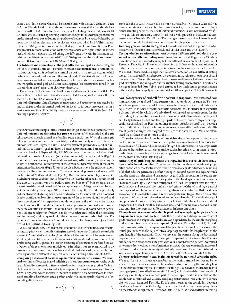
We calculated circularity scores for all trials with grid cells included in the cur-rent analysis (Extended Data Fig. 4). The average score was calculated for each mod-ule. A two-sample t-test was used to compare the degree of circularity.Defining grid cell modules. A grid cell module was defined as a group of anato-mically neighbouring grid cells which had similar scale and orientation25.Testing whether relative orientations between different grid modules are pre-served across different testing conditions. We looked at 18 grid cells (3 rats, 6modules in each rat) recorded in up to three different environments (Fig. 2c–e andExtended Data Fig. 5). The relative orientation is defined as the mean orientationdifference between closest components of two simultaneously recorded modules.We asked if these modules kept their relative orientation across different testingarenas, that is, the difference between the corresponding relative orientations shouldbe close to zero. To test this we calculated the mean difference between the relativegrid orientations in the square and in another testing environment (a circle or ahexagon; Extended Data Table 1) and estimated how likely it is to get such a meandifference by chance applying the binomial test (the range of available differences is0u–30u).Non-homogeneity of grid cell firing pattern in trapezoids. We examined howhomogeneous the grid cell firing pattern is in trapezoids versus squares. To mea-sure homogeneity we divided the enclosures into two parts (left and right) withequal areas (in the case of the trapezoid its horizontal axis is divided into segments64% and 36% of the whole). We calculated local spatial autocorrelograms for theleft and right parts of the trapezoid and square separately. To evaluate the degree ofsimilarity between the left and the right parts of the environment (square or trap-ezoid) we calculated the Pearson product-moment correlation coefficient betweenthem. If the sizes of local spatial autocorrelograms were different between the dif-ferent parts, the larger was cropped to the size of the smaller one. We also calcu-lated the gridness score for each of them.

The orientation and scale on the left and right sides of the trapezoidal and squareenclosures were evaluated from the local spatial autocorrelogram of each side (seethe section on field size and orientation of the grid cells for details). The componentsclosest to the horizontal axis were considered the first grid cell component, the sec-ond component was that at the closest angle in anti-clockwise direction followedby the third (Extended Data Fig. 6).Anisotropy of grid firing pattern in the trapezoid does not result from inade-quate behavioural sampling. To examine whether the changes in grid cell prop-erties on the left part of the trapezoid resulted from inadequate behavioural samplingof the left side, we generated a perfect homogeneous grid pattern in a square whichhad the same wavelength and orientation as grid cells recorded in the square en-vironment as estimated from the six peaks of the local spatial autocorrelogram(Extended Data Fig. 7). We then transposed this idealized pattern onto the trape-zoidal shape and measured the similarity and gridness of the left and right parts ofthe trapezoid and found no difference in gridness, demonstrating that the differ-ences seen in the real data are not due to inadequate sampling on the left side of thetrapezoid. We also found the orientations and wavelengths of the main three gridcomponents of simulated grid patterns in the left and right sides of a trapezoid anda square and showed that they had much smaller differences than observed in ourdata and that they were not different across different directions.Change in symmetry cannot be simply predicted by morphing the pattern froma square to a trapezoid. We tested whether the observed change in symmetry ofgrids recorded in a trapezoidal enclosure can be predicted by the simple morphingof the pattern from a square to a trapezoid (Extended Data Figs 8 and 9). To esti-mate how grid pattern in a square would appear in a trapezoid, we expanded theinitial grid pattern in the square into a larger square with the length equal to thelong length of the trapezoid. Then we rescaled the pattern along the horizontaltrapezoid axis to match the size of the original trapezoid (similar to ref. 26). The cor-relation coefficients between the predicted versus recorded grid patterns were usedto estimate how well our transformation matched the experimentally measuredpattern. The distribution is not significantly different from the normal distributionwith a mean equal to zero (P 5 0.74, t 5 20.33, df 5 36, one-sample t-test).Comparing behavioural biases in the left part of the trapezoid versus the right.We used the same analysis as described in the section entitled comparing beha-vioural biases in square versus circular enclosures for comparing the sampling biason the left side of the trapezoid with that on the right. We divided the trapezoid intotwo equal parts (area of half-trapezoid, 0.51 m2) and calculated the directional andvelocity circularity scores for each part. A two-sample t-test revealed that on thewhole both directional and velocity sampling distributions were different betweenthe two parts (Extended Data Fig. 4). We then measured the correlation betweenthe degree of similarity of the local grid pattern and the difference in sampling biaseson the left and the right sides (Extended Data Fig. 4e, f). We showed that there is no

LETTER RESEARCH

Macmillan Publishers Limited. All rights reserved©2015

significant correlation between these measures suggesting that observed grid non-homogeneity in the trapezoid did not result from the difference in directional or ve-locity sampling distributions.

22. Skaggs, W. E., McNaughton, B. L., Gothard, K. M. & Markus, E. J. An Information-Theoretic Approach to Deciphering the Hippocampal Code 1030–1037 (MorganKaufmann, 1993).

23. Wills, T. J., Cacucci, F., Burgess, N. & O’Keefe, J. Development of the hippocampalcognitive map in preweanling rats. Science 328, 1573–1576 (2010).

24. Hafting, T., Fyhn, M., Molden, S., Moser, M.-B. & Moser, E. I. Microstructure of aspatial map in the entorhinal cortex. Nature 436, 801–806 (2005).

25. Stensola, H. et al. The entorhinal grid map is discretized. Nature 492, 72–78(2012).

26. Barry, C., Hayman, R., Burgess, N. & Jeffery, K. J. Experience-dependent rescalingof entorhinal grids. Nature Neurosci. 10, 682–684 (2007).

RESEARCH LETTER

Macmillan Publishers Limited. All rights reserved©2015

Extended Data Figure 1 | Sagittal Nissl-stained brain sections showing therecording locations in superficial layers II-III of mEC and PaS.a–s,Yellow dots indicate the dorsal-ventral region where grid cells were

recorded in the trapezoids. PAS marked with asterisk symbols. Scale bar,500mm.

LETTER RESEARCH

Macmillan Publishers Limited. All rights reserved©2015

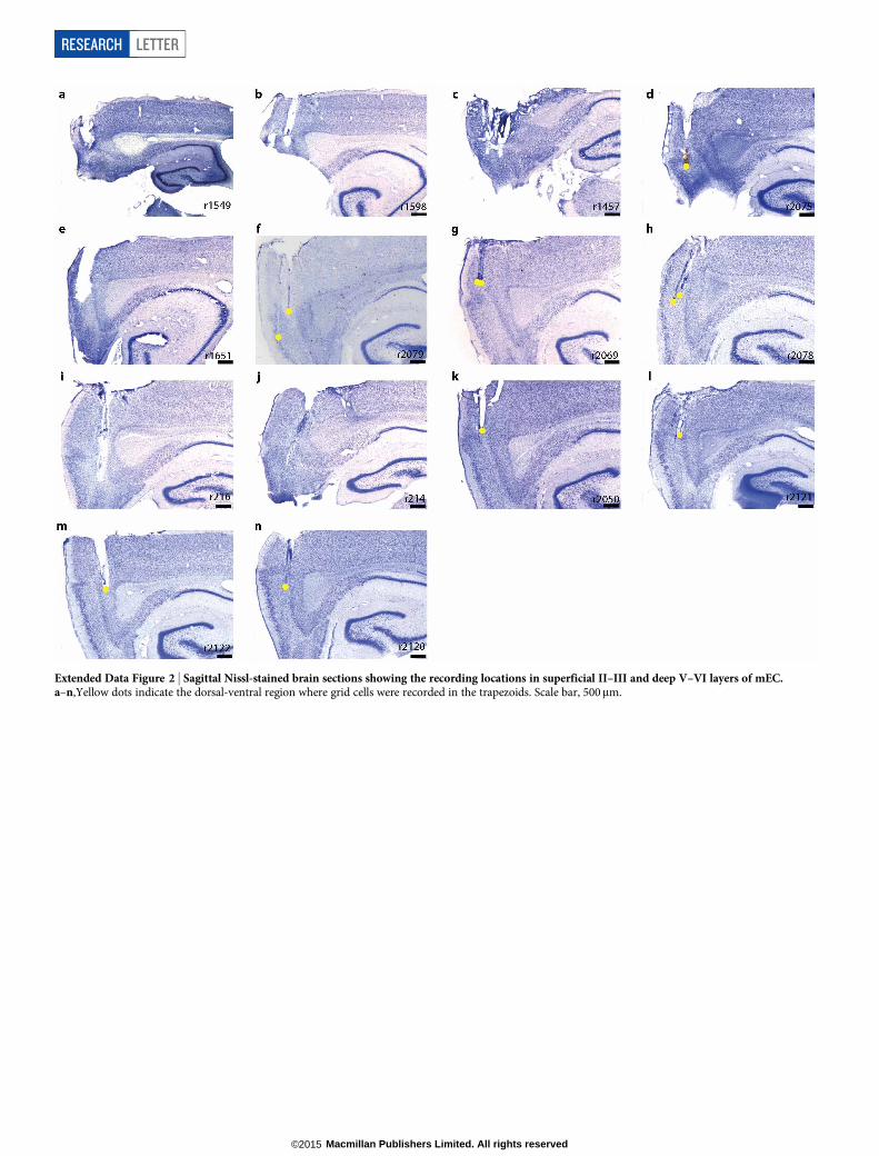
Extended Data Figure 2 | Sagittal Nissl-stained brain sections showing the recording locations in superficial II–III and deep V–VI layers of mEC.a–n,Yellow dots indicate the dorsal-ventral region where grid cells were recorded in the trapezoids. Scale bar, 500mm.

RESEARCH LETTER

Macmillan Publishers Limited. All rights reserved©2015

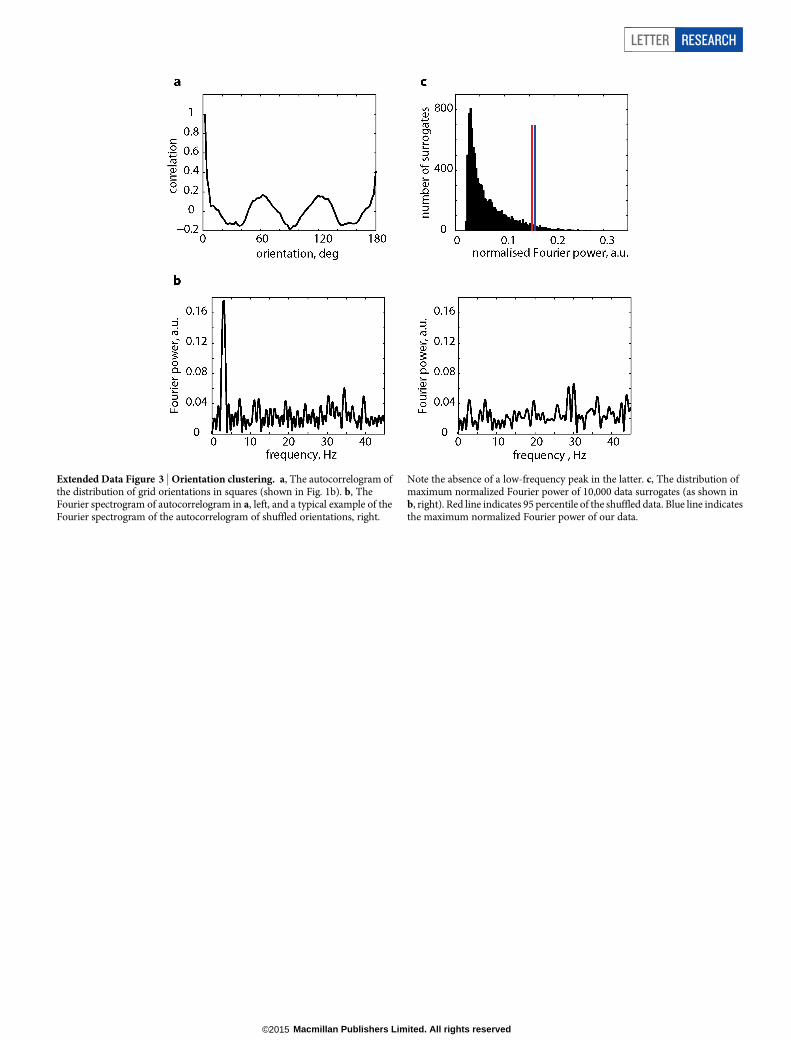
Extended Data Figure 3 | Orientation clustering. a, The autocorrelogram ofthe distribution of grid orientations in squares (shown in Fig. 1b). b, TheFourier spectrogram of autocorrelogram in a, left, and a typical example of theFourier spectrogram of the autocorrelogram of shuffled orientations, right.

Note the absence of a low-frequency peak in the latter. c, The distribution ofmaximum normalized Fourier power of 10,000 data surrogates (as shown inb, right). Red line indicates 95 percentile of the shuffled data. Blue line indicatesthe maximum normalized Fourier power of our data.

LETTER RESEARCH

Macmillan Publishers Limited. All rights reserved©2015

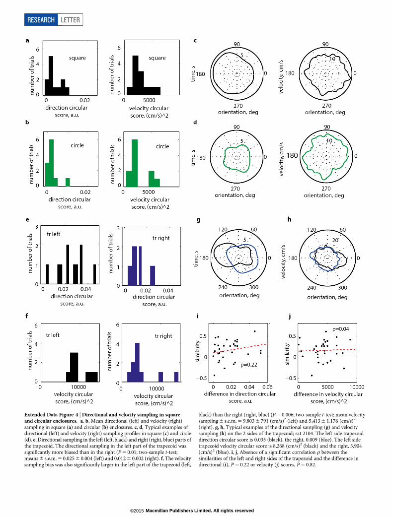
Extended Data Figure 4 | Directional and velocity sampling in squareand circular enclosures. a, b, Mean directional (left) and velocity (right)sampling in square (a) and circular (b) enclosures. c, d, Typical examples ofdirectional (left) and velocity (right) sampling profiles in square (c) and circle(d). e, Directional sampling in the left (left, black) and right (right, blue) parts ofthe trapezoid. The directional sampling in the left part of the trapezoid wassignificantly more biased than in the right (P 5 0.01; two-sample t-test;means 6 s.e.m. 5 0.025 6 0.004 (left) and 0.012 6 0.002 (right). f, The velocitysampling bias was also significantly larger in the left part of the trapezoid (left,

black) than the right (right, blue) (P 5 0.006; two-sample t-test; mean velocitysampling 6 s.e.m. 5 9,803 6 791 (cm/s)2 (left) and 5,413 6 1,176 (cm/s)2

(right). g, h, Typical examples of the directional sampling (g) and velocitysampling (h) on the 2 sides of the trapezoid; rat 2104. The left side trapezoiddirection circular score is 0.035 (black), the right, 0.009 (blue). The left sidetrapezoid velocity circular score is 8,268 (cm/s)2 (black) and the right, 3,904(cm/s)2 (blue). i, j, Absence of a significant correlation r between thesimilarities of the left and right sides of the trapezoid and the difference indirectional (i), P 5 0.22 or velocity (j) scores, P 5 0.82.

RESEARCH LETTER

Macmillan Publishers Limited. All rights reserved©2015

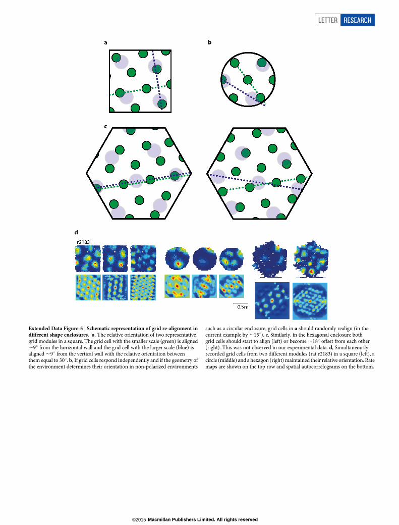
Extended Data Figure 5 | Schematic representation of grid re-alignment indifferent shape enclosures. a, The relative orientation of two representativegrid modules in a square. The grid cell with the smaller scale (green) is aligned,9u from the horizontal wall and the grid cell with the larger scale (blue) isaligned ,9u from the vertical wall with the relative orientation betweenthem equal to 30u. b, If grid cells respond independently and if the geometry ofthe environment determines their orientation in non-polarized environments

such as a circular enclosure, grid cells in a should randomly realign (in thecurrent example by ,15u). c, Similarly, in the hexagonal enclosure bothgrid cells should start to align (left) or become ,18u offset from each other(right). This was not observed in our experimental data. d, Simultaneouslyrecorded grid cells from two different modules (rat r2183) in a square (left), acircle (middle) and a hexagon (right) maintained their relative orientation. Ratemaps are shown on the top row and spatial autocorrelograms on the bottom.

LETTER RESEARCH

Macmillan Publishers Limited. All rights reserved©2015

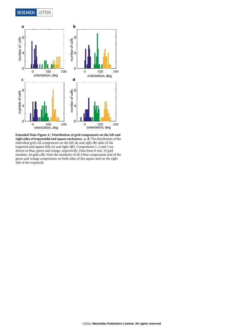
Extended Data Figure 6 | Distribution of grid components on the left andright sides of trapezoidal and square enclosures. a–d, The distribution of theindividual grid cell components on the left (a) and right (b) sides of thetrapezoid and square (left (c) and right (d)). Components 1, 2 and 3 areshown in blue, green and orange, respectively. Data from 8 rats, 10 gridmodules, 26 grid cells. Note the similarity of all 4 blue components and of thegreen and orange components on both sides of the square and on the rightside of the trapezoid.

RESEARCH LETTER

Macmillan Publishers Limited. All rights reserved©2015

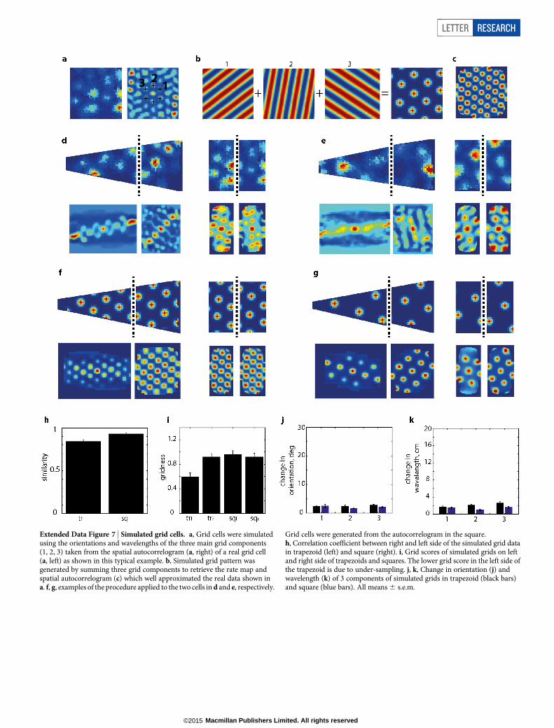
Extended Data Figure 7 | Simulated grid cells. a, Grid cells were simulatedusing the orientations and wavelengths of the three main grid components(1, 2, 3) taken from the spatial autocorrelogram (a, right) of a real grid cell(a, left) as shown in this typical example. b, Simulated grid pattern wasgenerated by summing three grid components to retrieve the rate map andspatial autocorrelogram (c) which well approximated the real data shown ina. f, g, examples of the procedure applied to the two cells in d and e, respectively.

Grid cells were generated from the autocorrelogram in the square.h, Correlation coefficient between right and left side of the simulated grid datain trapezoid (left) and square (right). i, Grid scores of simulated grids on leftand right side of trapezoids and squares. The lower grid score in the left side ofthe trapezoid is due to under-sampling. j, k, Change in orientation (j) andwavelength (k) of 3 components of simulated grids in trapezoid (black bars)and square (blue bars). All means 6 s.e.m.

LETTER RESEARCH

Macmillan Publishers Limited. All rights reserved©2015

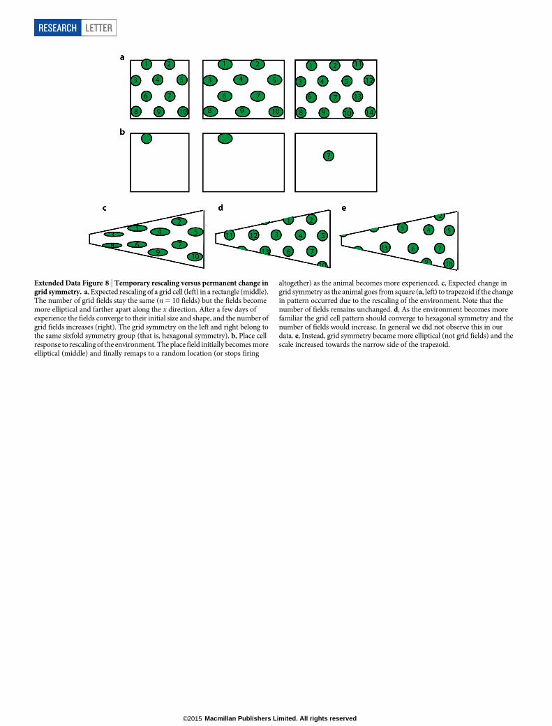
Extended Data Figure 8 | Temporary rescaling versus permanent change ingrid symmetry. a, Expected rescaling of a grid cell (left) in a rectangle (middle).The number of grid fields stay the same (n 5 10 fields) but the fields becomemore elliptical and farther apart along the x direction. After a few days ofexperience the fields converge to their initial size and shape, and the number ofgrid fields increases (right). The grid symmetry on the left and right belong tothe same sixfold symmetry group (that is, hexagonal symmetry). b, Place cellresponse to rescaling of the environment. The place field initially becomes moreelliptical (middle) and finally remaps to a random location (or stops firing

altogether) as the animal becomes more experienced. c, Expected change ingrid symmetry as the animal goes from square (a, left) to trapezoid if the changein pattern occurred due to the rescaling of the environment. Note that thenumber of fields remains unchanged. d, As the environment becomes morefamiliar the grid cell pattern should converge to hexagonal symmetry and thenumber of fields would increase. In general we did not observe this in ourdata. e, Instead, grid symmetry became more elliptical (not grid fields) and thescale increased towards the narrow side of the trapezoid.

RESEARCH LETTER

Macmillan Publishers Limited. All rights reserved©2015

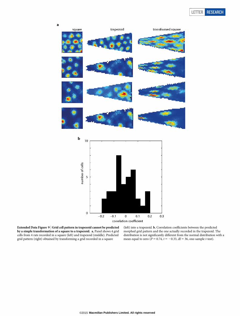
Extended Data Figure 9 | Grid cell pattern in trapezoid cannot be predictedby a simple transformation of a square to a trapezoid. a, Panel shows 4 gridcells from 4 rats recorded in a square (left) and trapezoid (middle). Predictedgrid pattern (right) obtained by transforming a grid recorded in a square

(left) into a trapezoid. b, Correlation coefficients between the predictedmorphed grid pattern and the one actually recorded in the trapezoid. Thedistribution is not significantly different from the normal distribution with amean equal to zero (P 5 0.74, t 5 20.33, df 5 36, one-sample t-test).

LETTER RESEARCH

Macmillan Publishers Limited. All rights reserved©2015

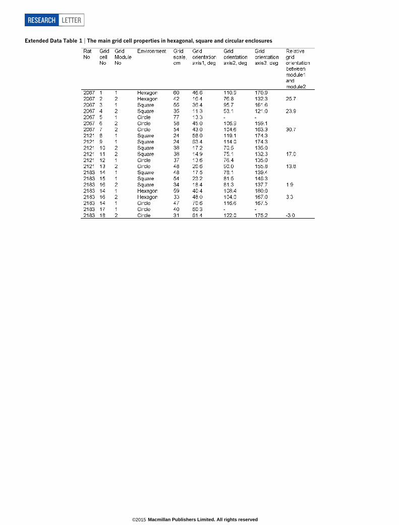
Extended Data Table 1 | The main grid cell properties in hexagonal, square and circular enclosures

RESEARCH LETTER

Macmillan Publishers Limited. All rights reserved©2015