Greyscale - density calibration of an industrial CT scanner for ...

GREYSCALE - DENSITY CALIBRATION OF AN INDUSTRIAL CT SCANNER

FOR WOOD MICRODENSITOMETRY

by Marios Kadas

Thesis presented in fulfilment of the requirements for the degree of Master of Science in Forestry in the Faculty of

Forest and Wood Science at Stellenbosch University

Supervisor: Prof Thomas Seifert Co-supervisor: Prof Martina Meincken

March 2016

Declaration

By submitting this thesis/dissertation electronically, I declare that the entirety of the work contained therein is my own, original work, that I am the sole author thereof (save to the extent explicitly otherwise stated), that reproduction and publication thereof by Stellenbosch University will not infringe any third party rights and that I have not previously in its entirety or in part submitted it for obtaining any qualification.

March 2016

Copyright © 2016 Stellenbosch University All rights reserved

Stellenbosch University https://scholar.sun.ac.za

Abstract The microdensitometry of wood, that is the quantification of density in the micrometre scale, is important for different scientific disciplines such as wood science, dendrochronology, dendroecology, dendroclimatology, and biomass determination and in the industrial applications of engineered wood. With the advent of industrial computed tomography scanners, powerful equipment for density measurement is available. However, the methodological framework for wood density determination with those machines is not fully established, because possible error sources have not so far been analysed and described sufficiently. Thus, the objective of this study was the development of a methodology, in order to quantify wood density with an industrial computed tomography scanner. In this study, industrial cone-beam computed tomography was used for the microdensitometry of wood. Fifty stacks of stem discs from an equal number of Pinus radiata trees were used as the sample dataset. Firstly, the fifty stacks were scanned along with selected reference materials, which were measured for density in a conventional way. Then, fifty linear regressions were performed between the conventionally-determined density and the grey value of the reference materials. A strong correlation (mean R2=0.998) between conventionally-determined density and grey value was observed. The regressions also provided calibration equations, which could translate a given grey value to a certain density. For validation purposes, the fifty calibration equations were tested on extra reference materials. The density from the computed tomography scanner had a mean absolute error of 0.008 g/cm3 (σ=0.004) and a mean percent error of 1.4% (σ=0.7). Additionally, one of the calibration equations was applied to the creation of tree ring density profiles. An important result of the study was that it was not possible to deduce a sole calibration equation, as typically done with densitometers and medical computed tomography scanners. Thus, the calibration of each scan was inevitable, due to the various degrees of freedom of the industrial computed tomography scanner.


Opsomming Die mikrodensitometrie van hout, dws die kwantifisering van die digtheid op die mikrometer skaal is belangrik vir verskillende wetenskaplike dissiplines soos houtwetenskap, dendro-chronologie, dendro-ekologie, dendro-klimatologie, biomassa bepaling en vir die industriële gebruik van verwerkte hout. Met die koms van die industriële tomografie skandeerders is kragtige toerusting vir die meting van houtdigtheid beskikbaar. Die metodologiese raamwerk vir die bepaling van hout digtheid met die masjiene is egter nog nie ten volle ontwikkel nie. Dit kan aanleiding gee tot metingsfoute wat nie voldoende geanaliseer en beskryf word nie. Die doel van hierdie studie is dus om ‘n metode te ontwikkel om houtdigtheid te kwantifiseer deur die gebruik van ‘n industriële tomografie-skandeerder. In hierdie studie is industriële laser ligstraal tomografie gebruik om die mikrodensitometrie van hout te bepaal. Vir die monster datastel is vyftig stapels van die stam skywe van 'n gelyke aantal Pinus radiata bome gebruik. Eerstens is die vyftig stapels geskandeer saam met geselekteerde verwysingsmateriaal wat vir digtheid gemeet is op 'n konvensionele manier. Daarna is vyftig lineêre regressies ontwikkel tussen die digtheid wat bepaal is deur die konvensionele digtheidsmetode en die grys waarde van die verwysing materiaal. Met die studie is waargeneem dat daar ‘n sterk korrelasie (R² = 0.998) is tussen die digtheid gemeet deur die gebruik van die konvensionele metode en die gryswaarde. Die regressies voorsien ook kalibrasie vergelykings, wat 'n gegewe grys waarde kan assosieer met 'n sekere digtheid. Vir validerings doeleindes, is die vyftig kalibrasie vergelykings getoets op ekstra verwysingsmateriaal. Die digtheid gemeet deur die tomografie-skandeerder het 'n gemiddelde absolute afwyking van 0.008 g/cm³ (σ=0.004) en 'n gemiddelde 1.4% (σ=0.7) fout getoon. Verder is een van die ontwikkelde kalibrasie vergelykings toegepas om boomring digtheidsprofiele te skep. Die studie het bevind dat ‘n enkele kallibrasie vergelyking nie gebruik kan word soos tipies met die gebruik van densitometers en mediese tomografie skandeerders nie. Die industriële tomografie-skandeerder moes dus gekalibreer word met elke skandering as gevolg van die verskillende grade van vryheid wat bevind is in die studie.


Σύνοψη Η μικροπυκνομετρία του ξύλου, δηλαδή η ποσοτικοποίηση της πυκνότητας στην κλίμακα του μικρομέτρου, είναι σημαντική για διάφορα επιστημονικά πεδία όπως η επιστήμη του ξύλου, η δενδροχρονολογία, η δενδροοικολογία, η δενδροκλιματολογία, και ο καθορισμός της βιομάζας και σε βιομηχανικές εφαρμογές επεξεργασμένου ξύλου. Με την άφιξη των βιομηχανικών υπολογιστικών τομογράφων, ισχυρός εξοπλισμός για τη μέτρηση της πυκνότητας είναι διαθέσιμος. Παρ’ όλα αυτά, το μεθοδολογικό πλαίσιο για τον καθορισμό της πυκνότητας του ξύλου με αυτά τα μηχανήματα δεν είναι πλήρως εδραιωμένο, επειδή πιθανές πηγές σφάλματος δεν έχουν μέχρι στιγμής αναλυθεί και περιγραφεί επαρκώς. Συνεπώς, το αντικείμενο αυτής της μελέτης ήταν η ανάπτυξη μιας μεθοδολογίας, ώστε να ποσοτικοποιηθεί η πυκνότητα του ξύλου με ένα βιομηχανικό υπολογιστικό τομογράφο. Σε αυτήν τη μελέτη, η βιομηχανική υπολογιστική τομογραφία κωνικής δέσμης χρησιμοποιήθηκε για τη μικροπυκνομετρία του ξύλου. Πενήντα στοίβες δίσκων κορμών από ένα ίσο αριθμό δέντρων Pinus radiata χρησιμοποιήθηκαν ως δείγμα δεδομένων. Αρχικά, οι πενήντα στοίβες σκαναρίστηκαν μαζί με επιλεγμένα υλικά αναφοράς, στα οποία μετρήθηκε η πυκνότητα με συμβατικό τρόπο. Μετά, πενήντα γραμμικές παλινδρομήσεις έγιναν μεταξύ της συμβατικά-καθορισμένης πυκνότητας και της τιμής του γκρι των υλικών αναφοράς. Παρατηρήθηκε μια ισχυρή συσχέτιση (μέσος όρος των R2=0.998) μεταξύ της συμβατικά-καθορισμένης πυκνότητας και της τιμής του γκρι. Οι παλινδρομήσεις επίσης παρείχαν εξισώσεις καλιμπραρίσματος, οι οποίες μπορούσαν να μεταφράσουν μια δοθείσα τιμή του γκρι σε μια συγκεκριμένη πυκνότητα. Για λόγους επαλήθευσης, οι πενήντα εξισώσεις καλιμπραρίσματος δοκιμάστηκαν σε έξτρα υλικά αναφοράς. Η πυκνότητα από τον υπολογιστικό τομογράφο είχε μέσο απόλυτο σφάλμα 0.008 g/cm3 (σ=0.004) και μέσο τοις εκατό σφάλμα 1.4% (σ=0.7). Επιπροσθέτως, μία από τις εξισώσεις καλιμπραρίσματος εφαρμόστηκε στην δημιουργία προφίλ πυκνότητας δακτυλίων δέντρων. Ένα σημαντικό αποτέλεσμα της μελέτης ήταν ότι δεν ήταν δυνατόν να χρησιμοποιηθεί μια μοναδική εξίσωση καλιμπραρίσματος, όπως τυπικά γίνεται με τους πυκνομετρητές και τους ιατρικούς υπολογιστικούς τομογράφους. Συνεπώς, το καλιμπράρισμα του κάθε σκαναρίσματος ήταν αναπόφευκτο, εξαιτίας των διαφόρων βαθμών ελευθερίας του βιομηχανικού υπολογιστικού τομογράφου.


Acknowledgements I would like to acknowledge: Prof Thomas Seifert for his unique guidance throughout the project. Dr Anton du Plessis for his great amount of personal contribution to the design and the realization of the CT scanner experiments. Dr Martina Meincken for her useful advice. Mr Mark February, Mr Wilmour Hendrikse, and Mr Yos Weerdenburg for the cut of the imaging phantom. Mr Otto Pienaar for the translation of the abstract. Mr Phillip Fischer for the P. radiata samples. Ms Angeline Atsame-Edda, Ms Dorothea van Vuuren, Mr Emile Kitenge, Mr Robert Mupemba, Dr Benedict Ohdiambo and Ms Ursula Petersen for their great help with the project. NRF/BMBF-project FORSIM and the EU Marie Curie IRSEs project: “Climate Fit Forests” for the financial support for sampling and CT scanning.


i

Table of Contents List of Tables ........................................................................................................................... iii List of Figures .......................................................................................................................... iv List of Equations ....................................................................................................................... v List of Abbreviations ................................................................................................................ vi 1. Introduction ........................................................................................................................ 1

1.1. X-ray computed tomography ....................................................................................... 1 1.1.1. Principle of operation ............................................................................................ 1 1.1.2. Linear attenuation coefficient ................................................................................ 2 1.1.3. CT numbers .......................................................................................................... 3

1.2. CT densitometry .......................................................................................................... 3 1.3. Motivation .................................................................................................................... 4 1.4. Identification of gaps of knowledge .............................................................................. 5

2. Materials and Methods ...................................................................................................... 7 2.1. Overall objective .......................................................................................................... 7 2.2. Summary of the methodology ...................................................................................... 7 2.3. Imaging phantom and wood samples .......................................................................... 9 2.4. CT scanning procedure ............................................................................................. 11 2.5. Greyscale - density calibration ................................................................................... 16 2.6. Tree ring CT density profile ....................................................................................... 20 2.7. Potential sources of CT density error ......................................................................... 23

2.7.1. Homogeneity of phantom slices .......................................................................... 23 2.7.2. Number of phantom slices................................................................................... 23

3. Results ............................................................................................................................. 24 3.1. Greyscale - density calibration ................................................................................... 24 3.2. Tree ring CT density profile ....................................................................................... 29


ii

3.3. Potential sources of CT density error ......................................................................... 32 3.3.1. Homogeneity of phantom slices .......................................................................... 32 3.3.2. Number of phantom slices................................................................................... 32

4. Discussion ....................................................................................................................... 33 4.1. Accuracy and repeatability of the greyscale - density calibration ............................... 33

4.1.1. CT density error .................................................................................................. 33 4.1.2. Homogeneity of phantom slices .......................................................................... 33 4.1.3. Number of phantom slices................................................................................... 34 4.1.4. Chemical composition of phantom slices ............................................................ 34 4.1.5. Stability of the calibrations................................................................................... 35

4.2. Spatial accuracy ........................................................................................................ 35 4.3. Outlook on future work ............................................................................................... 36

5. Conclusions ..................................................................................................................... 38 6. Reference List ................................................................................................................. 39 Appendix A. Regression example ........................................................................................... 47 Appendix B. Regression results .............................................................................................. 48


iii

List of Tables Table 1 - The minimum, maximum and average diameter of the discs of each height 11 Table 2 - The settings of the scans 12 Table 3 - Example of a CT density profile table 21 Table 4 - Air-dry conventionally-determined density of the phantom slices 24 Table 5 - The mean CT density of each stem disc 29 Table 6 - Example of a regression dataset 47 Table 7 - The equations and the coefficients of determination of the regressions 48


iv

List of Figures Figure 1 - The configuration of an industrial cone beam CT scanner 1 Figure 2 - A synopsis of the methodology 8 Figure 3 - The imaging phantom 10 Figure 4 - A part of the Pinus radiata stacks which were used for testing the method 10 Figure 5 - An X-ray image from a CT scan 13 Figure 6 - A reconstructed volume 14 Figure 7 - A cross-section of a reconstructed volume 15 Figure 8 - A cross-sectional image with pseudocolour 17 Figure 9 - CT density profile selection on Image J 21 Figure 10, 11 and 12 - The effect of the strip width (1, 10, and 25 pixels) on the density profile 22 Figure 13 - One of the fifty greyscale - density regressions 25 Figure 14 - The dispersion of the calibration equations 26 Figure 15 - The frequency of reconstructed volumes per CT density error 28 Figure 16 - The frequency of reconstructed volumes per CT density error (%) 28 Figure 17 - The CT density profile of stem disc 1 29 Figure 18 - The CT density profile of stem disc 2 30 Figure 19 - The CT density profile of stem disc 3 30 Figure 20 - The CT density profile of stem disc 4 31 Figure 21 - The CT density profile of stem disc 5 31 Figure 22 - The confidence intervals of regressions with 4, 6, 8, 10, and 12 materials 32


v

List of Equations Equation 1 - The total linear attenuation coefficient 2 Equation 2 - The measured intensity of monochromatic radiation penetrating a homogeneous material 3 Equation 3 - Translation of a grey value into CT density 18 Equation 4 - The absolute error of the CT density of a phantom slice 19 Equation 5 - The percent error of the CT density of a phantom slice 19


vi

List of Abbreviations CT Computed tomography gv Grey value μ Linear attenuation coefficient ρC Density determined by conventional methods e.g. calliper and scale, water

displacement ρCT Density determined by a CT scanner σ Standard deviation of a population


1

1. Introduction 1.1. X-ray computed tomography

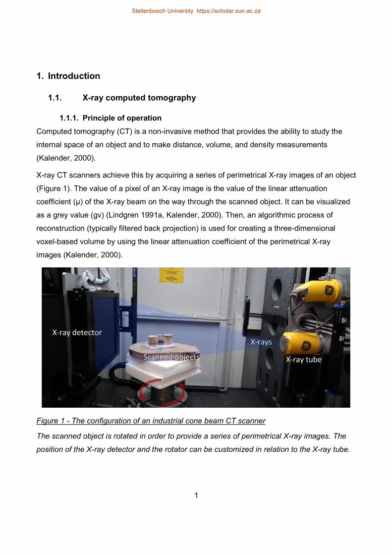
1.1.1. Principle of operation Computed tomography (CT) is a non-invasive method that provides the ability to study the internal space of an object and to make distance, volume, and density measurements (Kalender, 2000). X-ray CT scanners achieve this by acquiring a series of perimetrical X-ray images of an object (Figure 1). The value of a pixel of an X-ray image is the value of the linear attenuation coefficient (μ) of the X-ray beam on the way through the scanned object. It can be visualized as a grey value (gv) (Lindgren 1991a, Kalender, 2000). Then, an algorithmic process of reconstruction (typically filtered back projection) is used for creating a three-dimensional voxel-based volume by using the linear attenuation coefficient of the perimetrical X-ray images (Kalender, 2000).

Figure 1 - The configuration of an industrial cone beam CT scanner The scanned object is rotated in order to provide a series of perimetrical X-ray images. The position of the X-ray detector and the rotator can be customized in relation to the X-ray tube.


2

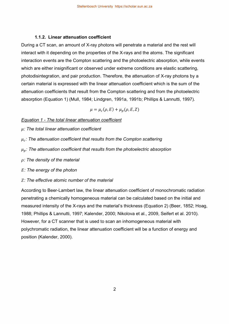
1.1.2. Linear attenuation coefficient During a CT scan, an amount of X-ray photons will penetrate a material and the rest will interact with it depending on the properties of the X-rays and the atoms. The significant interaction events are the Compton scattering and the photoelectric absorption, while events which are either insignificant or observed under extreme conditions are elastic scattering, photodisintegration, and pair production. Therefore, the attenuation of X-ray photons by a certain material is expressed with the linear attenuation coefficient which is the sum of the attenuation coefficients that result from the Compton scattering and from the photoelectric absorption (Equation 1) (Mull, 1984; Lindgren, 1991a, 1991b; Phillips & Lannutti, 1997).

= ( , ) + ( , , ) Equation 1 - The total linear attenuation coefficient

: The total linear attenuation coefficient : The attenuation coefficient that results from the Compton scattering : The attenuation coefficient that results from the photoelectric absorption

: The density of the material : The energy of the photon : The effective atomic number of the material

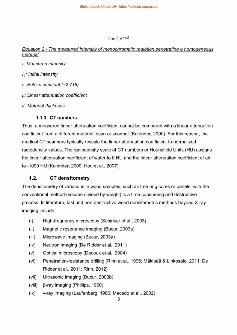
According to Beer-Lambert law, the linear attenuation coefficient of monochromatic radiation penetrating a chemically homogeneous material can be calculated based on the initial and measured intensity of the X-rays and the material’s thickness (Equation 2) (Beer, 1852; Hoag, 1988; Phillips & Lannutti, 1997; Kalender, 2000; Nikolova et al., 2009, Seifert et al. 2010). However, for a CT scanner that is used to scan an inhomogeneous material with polychromatic radiation, the linear attenuation coefficient will be a function of energy and position (Kalender, 2000).


3

= Equation 2 - The measured intensity of monochromatic radiation penetrating a homogeneous material : Measured intensity : Initial intensity : Euler’s constant (≈2.718) : Linear attenuation coefficient : Material thickness

1.1.3. CT numbers Thus, a measured linear attenuation coefficient cannot be compared with a linear attenuation coefficient from a different material, scan or scanner (Kalender, 2000). For this reason, the medical CT scanners typically rescale the linear attenuation coefficient to normalized radiodensity values. The radiodensity scale of CT numbers or Hounsfield Units (HU) assigns the linear attenuation coefficient of water to 0 HU and the linear attenuation coefficient of air to -1000 HU (Kalender, 2000; Hou et al., 2007).

1.2. CT densitometry The densitometry of variations in wood samples, such as tree ring cores or panels, with the conventional method (volume divided by weight) is a time-consuming and destructive process. In literature, fast and non-destructive wood densitometric methods beyond X-ray imaging include:

(i) High-frequency microscopy (Schinker et al., 2003) (ii) Magnetic resonance imaging (Bucur, 2003a) (iii) Microwave imaging (Bucur, 2003a) (iv) Neutron imaging (De Ridder et al., 2011) (v) Optical microscopy (Decoux et al., 2004) (vi) Penetration-resistance drilling (Rinn et al., 1996; Mäkipää & Linkosalo, 2011; De

Ridder et al., 2011; Rinn, 2012) (vii) Ultrasonic imaging (Bucur, 2003b) (viii) β-ray imaging (Phillips, 1960) (ix) γ-ray imaging (Laufenberg, 1986; Macedo et al., 2002)


4

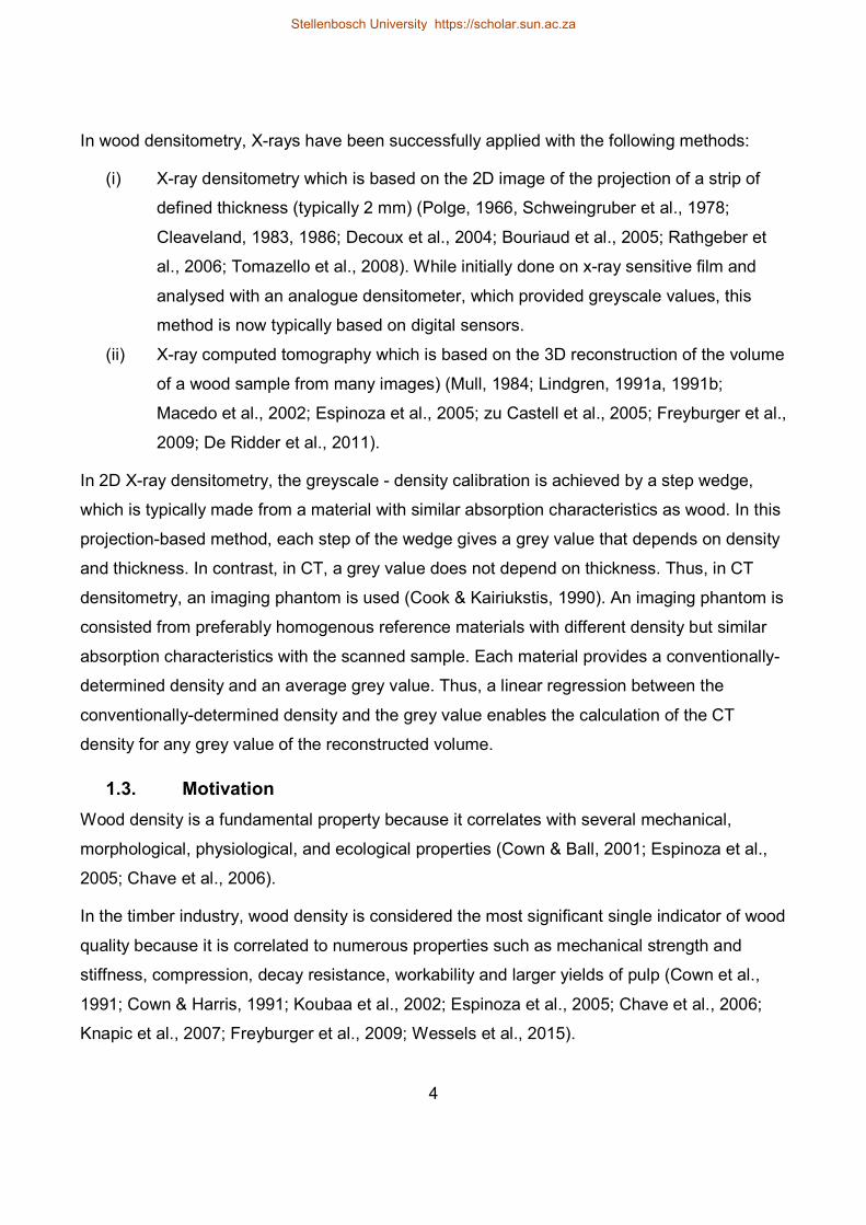
In wood densitometry, X-rays have been successfully applied with the following methods: (i) X-ray densitometry which is based on the 2D image of the projection of a strip of

defined thickness (typically 2 mm) (Polge, 1966, Schweingruber et al., 1978; Cleaveland, 1983, 1986; Decoux et al., 2004; Bouriaud et al., 2005; Rathgeber et al., 2006; Tomazello et al., 2008). While initially done on x-ray sensitive film and analysed with an analogue densitometer, which provided greyscale values, this method is now typically based on digital sensors.

(ii) X-ray computed tomography which is based on the 3D reconstruction of the volume of a wood sample from many images) (Mull, 1984; Lindgren, 1991a, 1991b; Macedo et al., 2002; Espinoza et al., 2005; zu Castell et al., 2005; Freyburger et al., 2009; De Ridder et al., 2011).

In 2D X-ray densitometry, the greyscale - density calibration is achieved by a step wedge, which is typically made from a material with similar absorption characteristics as wood. In this projection-based method, each step of the wedge gives a grey value that depends on density and thickness. In contrast, in CT, a grey value does not depend on thickness. Thus, in CT densitometry, an imaging phantom is used (Cook & Kairiukstis, 1990). An imaging phantom is consisted from preferably homogenous reference materials with different density but similar absorption characteristics with the scanned sample. Each material provides a conventionally-determined density and an average grey value. Thus, a linear regression between the conventionally-determined density and the grey value enables the calculation of the CT density for any grey value of the reconstructed volume.

1.3. Motivation Wood density is a fundamental property because it correlates with several mechanical, morphological, physiological, and ecological properties (Cown & Ball, 2001; Espinoza et al., 2005; Chave et al., 2006). In the timber industry, wood density is considered the most significant single indicator of wood quality because it is correlated to numerous properties such as mechanical strength and stiffness, compression, decay resistance, workability and larger yields of pulp (Cown et al., 1991; Cown & Harris, 1991; Koubaa et al., 2002; Espinoza et al., 2005; Chave et al., 2006; Knapic et al., 2007; Freyburger et al., 2009; Wessels et al., 2015).


5

In the context of global change, wood density is used to estimate the woody biomass of a forest in order to access the carbon storage of a forest source or of forest products (Chave et al., 2006; Freyburger et al., 2009; Seifert & Seifert, 2014; Magalhães & Seifert, 2015a; 2015b; Phiri et al., 2015). In engineered wood products such as wood fibre, particle, flake or veneer panels, the internal density variations determine their physical and mechanical properties like hardness, bending strength and stiffness, porosity, internal bond strength, holding strength of nails and screws (Laufenberg, 1986;) In the discipline of dendrochronology, wood density is also of great importance, since it provides additional contrast to optical tree ring measurements and additional parameters that can be correlated with climatic influences such as the latewood density (Cleaveland, 1986; Schweingruber & Kienast, 1986; Schweingruber, 1988; Cook & Kairiukstis, 1990; Briffa et al., 2002). In the broader sense of the term, dendrochronology includes many subdisciplines e.g. dendroarchaeology, dendrochemistry, dendroclimatology, dendroecology, dendroentomology, dendrogeomorphology, dendroglaciology, dendrohydrology, dendropyrochronology and dendroseismology (Fritts, 1976). Thus, for example, in dendroclimatology, wood density is considered a key parameter for climate reconstruction because of its strong correlation with climate (Hughes et al., 1984; D’Arrigo et al., 1992; Briffa et al., 1995; Briffa et al., 1998 cited in Bouriaud, et al., 2005). Furthermore, dendrochronology uses wood density profiles which are a series of consecutive density measurements from the innermost to the outermost tree ring. The density profiles can be used for ring-wise measurements (e.g. ring width, earlywood ring width, latewood ring width, latewood width percentage, average ring density, average earlywood density, average latewood density, ring density standard deviation) and for statistical modelling of density in relation to ring width, growth conditions etc. (Cleaveland, 1983; Koubaa et al., 2002; Nocetti et al., 2011).

1.4. Identification of gaps of knowledge The greyscale - density calibration can be influenced negatively by factors such as porosity, atomic numbers, quantum noise, artefacts related to topography, changes in the reconstruction algorithm, changes in the X-ray tube and the detector and aging of the X-ray tube (Phillips & Lannutti, 1997; Stoel et al., 2008). Most of the research studies were based


6

on medical CT scanners, which are quite limited in the ways the scan can be manipulated in terms of spatial resolution, voltage and current and thus are known to deliver quite homogeneous density results (Mull, 1984; Lindgren, 1991a, 1991b; Espinoza et al., 2005; Hou et al., 2007; Freyburger et al., 2009; Nikolova et al., 2009). In contrast, modern industrial cone beam CT scanners are fully customizable. The advent of industrial CT scanners has brought novel ways to analyse wood in terms of spatial and density resolution. However, there is not a standardized methodology of wood microdensitometry with industrial CT scanners to date, which substantially inhibits the comparability of results obtained with such machines.


7

2. Materials and Methods 2.1. Overall objective

To address the mentioned shortcomings, the research objective of this thesis was the contribution to the development of a robust methodology for accurate microdensitometry of wood samples with an industrial cone beam CT scanner. Within that context the study aimed at developing the methodological foundation for microdensitometry of Pinus radiata in a larger research project, so it was a logic choice to demonstrate the feasibility of the method on selected samples of that tree species. The main objective of this thesis was the development of an accurate and robust methodology for the greyscale - density calibration of reconstructed volumes of wood samples. As an additional objective, the greyscale - density calibration was applied for the creation of tree ring CT density profiles to show the feasibility of the method in radial density profiling. Further analysis of the density profiles from a forest and wood science perspective was beyond the goal of this study.

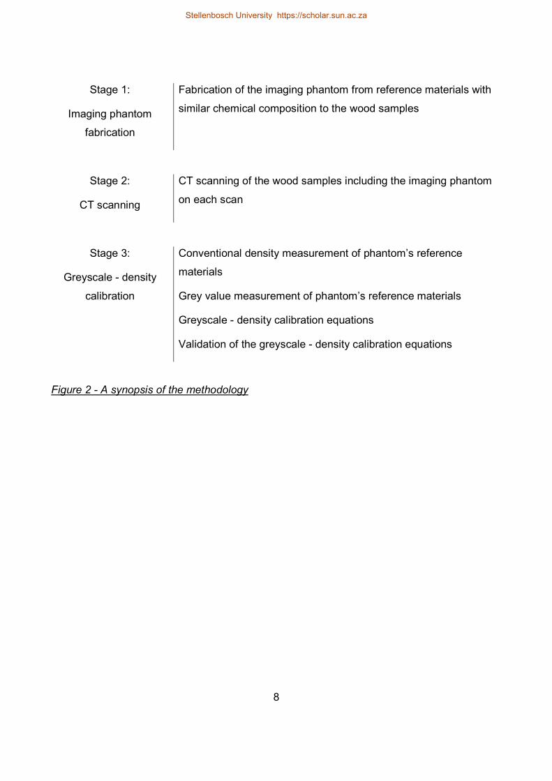
2.2. Summary of the methodology The methodology can be summarized as follows (Figure 2):

(i) The first stage of the methodology was the fabrication of an imaging phantom from reference materials with similar chemical composition to the wood samples. Stem discs of Pinus radiata were regarded as the wood samples.

(ii) The second stage was the CT scanning of the wood samples including the imaging phantom on each scan.

(iii) The third stage was the development of calibration equations that linked greyscale and density for each reconstructed volume. This was achieved by performing a regression between the conventionally-determined density and the grey value of the phantom’s reference materials. Then, the calibration was validated by calculating the error between the conventionally-determined density and the CT density of extra reference materials.


8

Stage 1: Imaging phantom

fabrication

Fabrication of the imaging phantom from reference materials with similar chemical composition to the wood samples

Stage 2:

CT scanning CT scanning of the wood samples including the imaging phantom on each scan

Stage 3:

Greyscale - density calibration

Conventional density measurement of phantom’s reference materials Grey value measurement of phantom’s reference materials Greyscale - density calibration equations Validation of the greyscale - density calibration equations

Figure 2 - A synopsis of the methodology


9

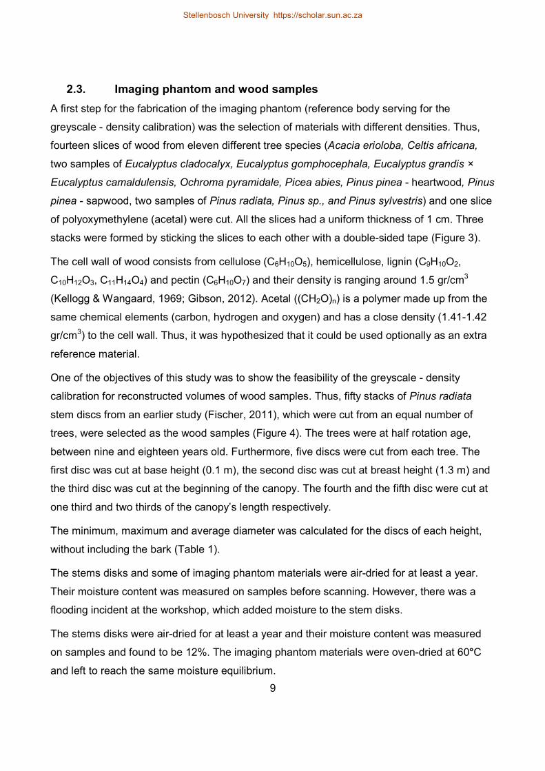
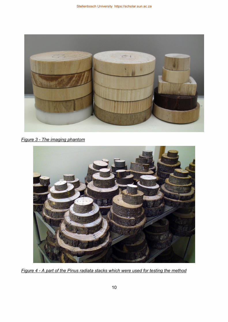
2.3. Imaging phantom and wood samples A first step for the fabrication of the imaging phantom (reference body serving for the greyscale - density calibration) was the selection of materials with different densities. Thus, fourteen slices of wood from eleven different tree species (Acacia erioloba, Celtis africana, two samples of Eucalyptus cladocalyx, Eucalyptus gomphocephala, Eucalyptus grandis × Eucalyptus camaldulensis, Ochroma pyramidale, Picea abies, Pinus pinea - heartwood, Pinus pinea - sapwood, two samples of Pinus radiata, Pinus sp., and Pinus sylvestris) and one slice of polyoxymethylene (acetal) were cut. All the slices had a uniform thickness of 1 cm. Three stacks were formed by sticking the slices to each other with a double-sided tape (Figure 3). The cell wall of wood consists from cellulose (C6H10O5), hemicellulose, lignin (C9H10O2, C10H12O3, C11H14O4) and pectin (C6H10O7) and their density is ranging around 1.5 gr/cm3 (Kellogg & Wangaard, 1969; Gibson, 2012). Acetal ((CH2O)n) is a polymer made up from the same chemical elements (carbon, hydrogen and oxygen) and has a close density (1.41-1.42 gr/cm3) to the cell wall. Thus, it was hypothesized that it could be used optionally as an extra reference material. One of the objectives of this study was to show the feasibility of the greyscale - density calibration for reconstructed volumes of wood samples. Thus, fifty stacks of Pinus radiata stem discs from an earlier study (Fischer, 2011), which were cut from an equal number of trees, were selected as the wood samples (Figure 4). The trees were at half rotation age, between nine and eighteen years old. Furthermore, five discs were cut from each tree. The first disc was cut at base height (0.1 m), the second disc was cut at breast height (1.3 m) and the third disc was cut at the beginning of the canopy. The fourth and the fifth disc were cut at one third and two thirds of the canopy’s length respectively. The minimum, maximum and average diameter was calculated for the discs of each height, without including the bark (Table 1). The stems disks and some of imaging phantom materials were air-dried for at least a year. Their moisture content was measured on samples before scanning. However, there was a flooding incident at the workshop, which added moisture to the stem disks. The stems disks were air-dried for at least a year and their moisture content was measured on samples and found to be 12%. The imaging phantom materials were oven-dried at 60°C and left to reach the same moisture equilibrium.


10

Figure 3 - The imaging phantom

Figure 4 - A part of the Pinus radiata stacks which were used for testing the method


11

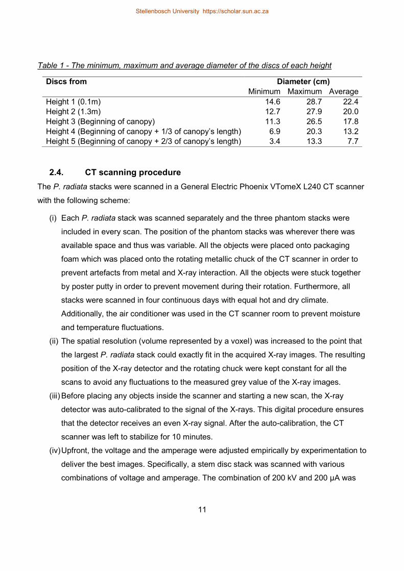
Table 1 - The minimum, maximum and average diameter of the discs of each height Discs from Diameter (cm) Minimum Maximum Average Height 1 (0.1m) 14.6 28.7 22.4 Height 2 (1.3m) 12.7 27.9 20.0 Height 3 (Beginning of canopy) 11.3 26.5 17.8 Height 4 (Beginning of canopy + 1/3 of canopy’s length) 6.9 20.3 13.2 Height 5 (Beginning of canopy + 2/3 of canopy’s length) 3.4 13.3 7.7

2.4. CT scanning procedure

The P. radiata stacks were scanned in a General Electric Phoenix VTomeX L240 CT scanner with the following scheme:

(i) Each P. radiata stack was scanned separately and the three phantom stacks were included in every scan. The position of the phantom stacks was wherever there was available space and thus was variable. All the objects were placed onto packaging foam which was placed onto the rotating metallic chuck of the CT scanner in order to prevent artefacts from metal and X-ray interaction. All the objects were stuck together by poster putty in order to prevent movement during their rotation. Furthermore, all stacks were scanned in four continuous days with equal hot and dry climate. Additionally, the air conditioner was used in the CT scanner room to prevent moisture and temperature fluctuations.

(ii) The spatial resolution (volume represented by a voxel) was increased to the point that the largest P. radiata stack could exactly fit in the acquired X-ray images. The resulting position of the X-ray detector and the rotating chuck were kept constant for all the scans to avoid any fluctuations to the measured grey value of the X-ray images.

(iii) Before placing any objects inside the scanner and starting a new scan, the X-ray detector was auto-calibrated to the signal of the X-rays. This digital procedure ensures that the detector receives an even X-ray signal. After the auto-calibration, the CT scanner was left to stabilize for 10 minutes.

(iv) Upfront, the voltage and the amperage were adjusted empirically by experimentation to deliver the best images. Specifically, a stem disc stack was scanned with various combinations of voltage and amperage. The combination of 200 kV and 200 μA was


12

selected because it provided the ideal brightness and contrast on the reconstruction of the disc stack. All further disc stacks were scanned with these parameters.

(v) Furthermore, a copper (Cu) (1mm) filter and an aluminium (Al) (1mm) filter were tested, but none was used for the scans because they affected the contrast.

(vi) The following parameters were set as shown on Table 2: Table 2 - The settings of the scans

Parameter Value Voltage 200 kV Amperage 200 μA Image resolution 2048×2048 Perimetrical images 3000 Image binning No Images acquired/skipped 1 acquired/1skipped Image exposure time 333ms Scan duration 36′ Region of Interest (ROI) Yes

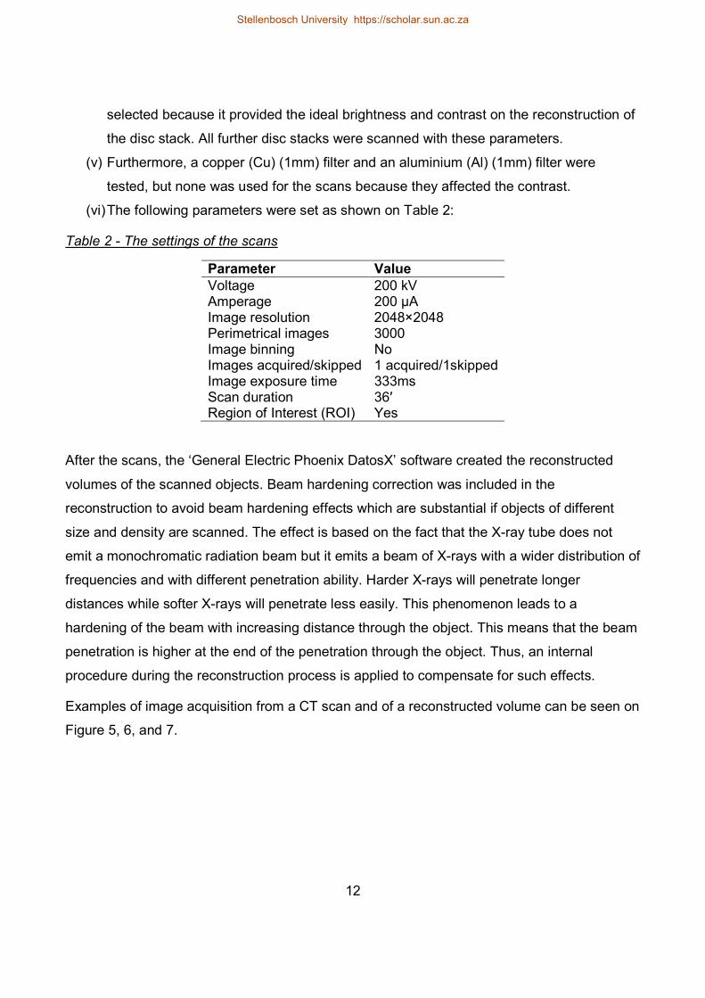
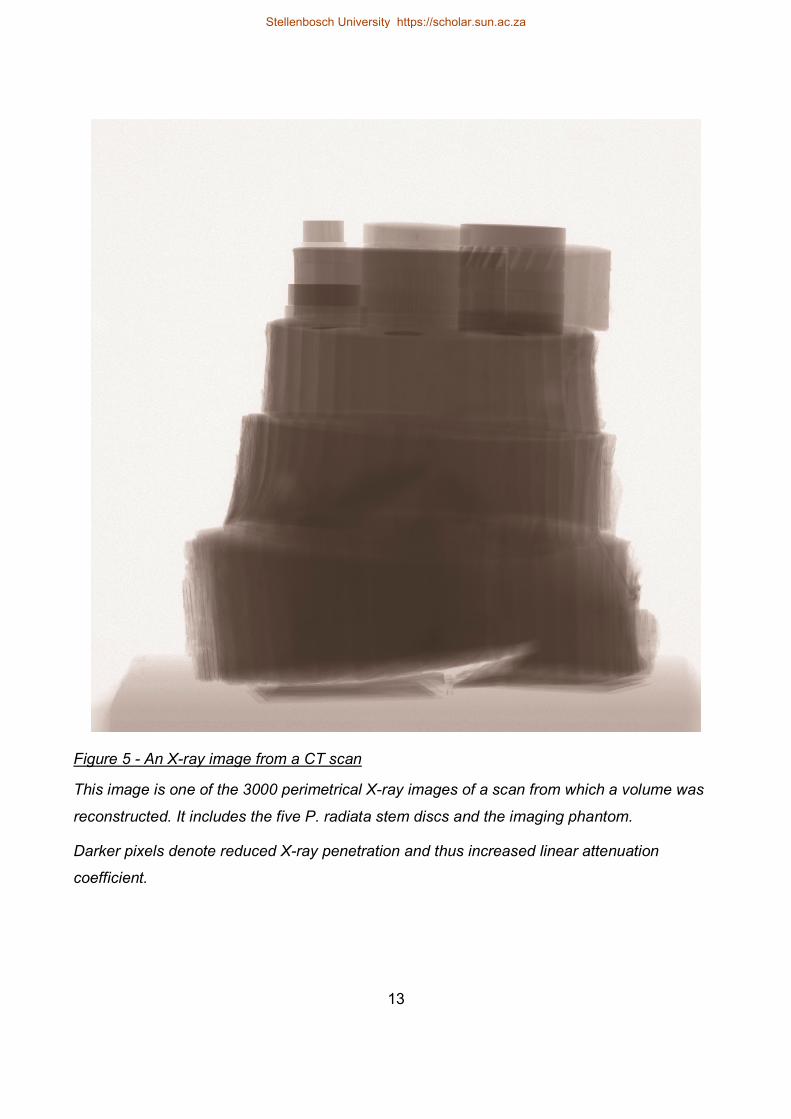
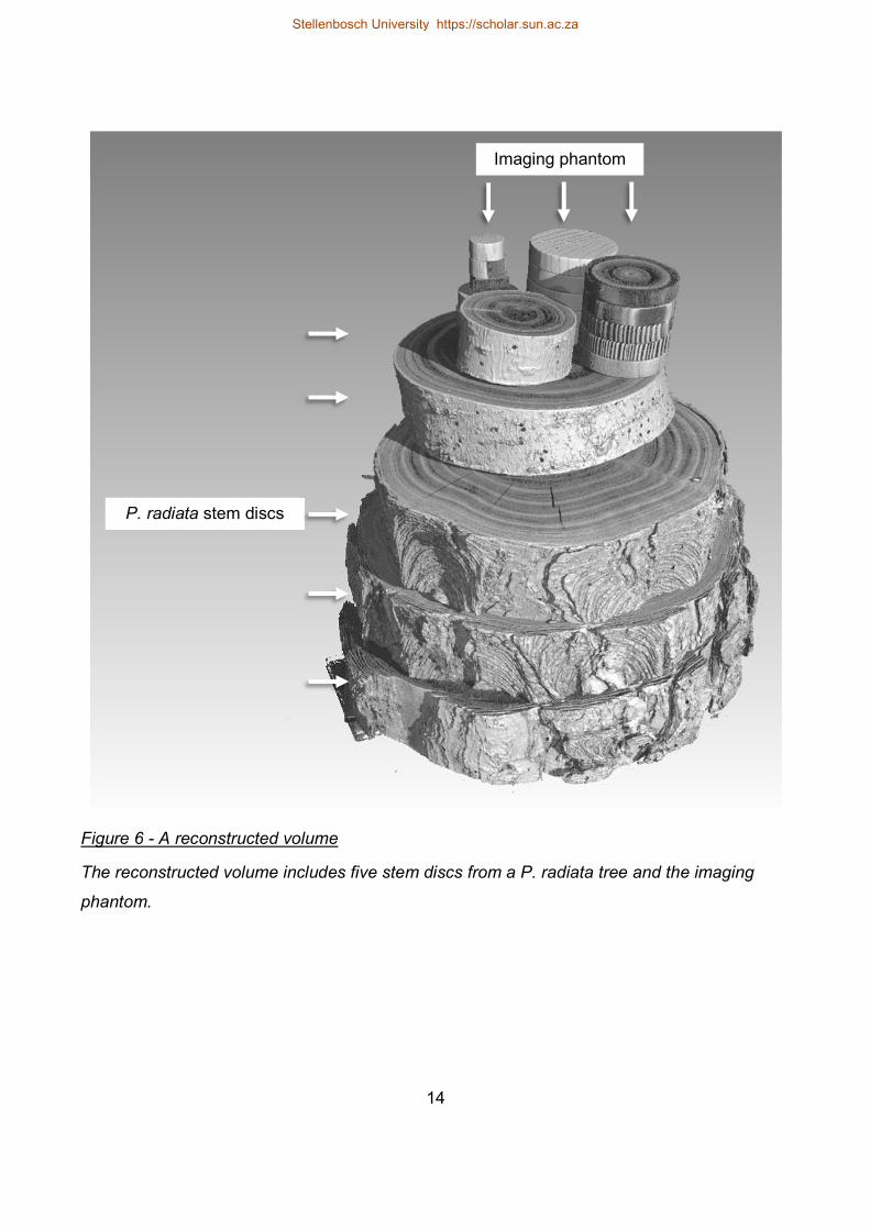
After the scans, the ‘General Electric Phoenix DatosX’ software created the reconstructed volumes of the scanned objects. Beam hardening correction was included in the reconstruction to avoid beam hardening effects which are substantial if objects of different size and density are scanned. The effect is based on the fact that the X-ray tube does not emit a monochromatic radiation beam but it emits a beam of X-rays with a wider distribution of frequencies and with different penetration ability. Harder X-rays will penetrate longer distances while softer X-rays will penetrate less easily. This phenomenon leads to a hardening of the beam with increasing distance through the object. This means that the beam penetration is higher at the end of the penetration through the object. Thus, an internal procedure during the reconstruction process is applied to compensate for such effects. Examples of image acquisition from a CT scan and of a reconstructed volume can be seen on Figure 5, 6, and 7.


13

Figure 5 - An X-ray image from a CT scan This image is one of the 3000 perimetrical X-ray images of a scan from which a volume was reconstructed. It includes the five P. radiata stem discs and the imaging phantom. Darker pixels denote reduced X-ray penetration and thus increased linear attenuation coefficient.


14

Figure 6 - A reconstructed volume The reconstructed volume includes five stem discs from a P. radiata tree and the imaging phantom.

P. radiata stem discs

Imaging phantom


15

Figure 7 - A cross-section of a reconstructed volume Brighter pixels represent higher densities and darker pixels, lower densities.


16

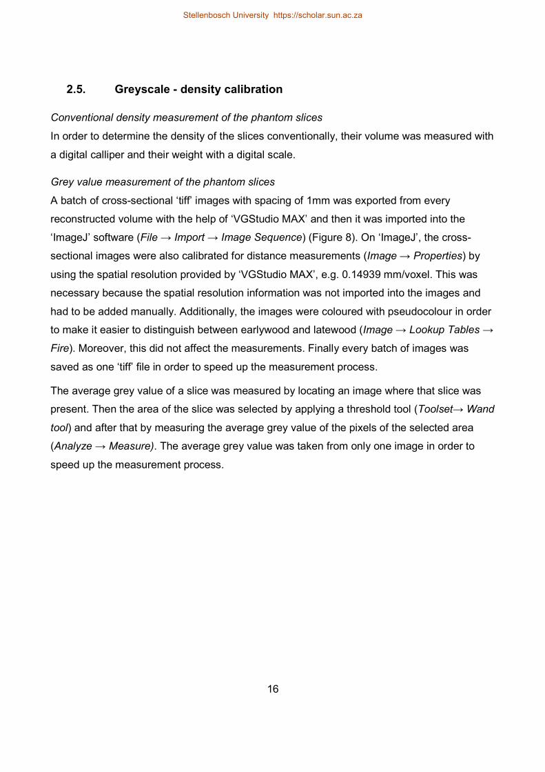
2.5. Greyscale - density calibration Conventional density measurement of the phantom slices In order to determine the density of the slices conventionally, their volume was measured with a digital calliper and their weight with a digital scale. Grey value measurement of the phantom slices A batch of cross-sectional ‘tiff’ images with spacing of 1mm was exported from every reconstructed volume with the help of ‘VGStudio MAX’ and then it was imported into the ‘ImageJ’ software (File → Import → Image Sequence) (Figure 8). On ‘ImageJ’, the cross-sectional images were also calibrated for distance measurements (Image → Properties) by using the spatial resolution provided by ‘VGStudio MAX’, e.g. 0.14939 mm/voxel. This was necessary because the spatial resolution information was not imported into the images and had to be added manually. Additionally, the images were coloured with pseudocolour in order to make it easier to distinguish between earlywood and latewood (Image → Lookup Tables → Fire). Moreover, this did not affect the measurements. Finally every batch of images was saved as one ‘tiff’ file in order to speed up the measurement process. The average grey value of a slice was measured by locating an image where that slice was present. Then the area of the slice was selected by applying a threshold tool (Toolset→ Wand tool) and after that by measuring the average grey value of the pixels of the selected area (Analyze → Measure). The average grey value was taken from only one image in order to speed up the measurement process.


17

Figure 8 - A cross-sectional image with pseudocolour A P. radiata stem disk and three phantom slices are visible. The values of the pixels increase from 0 to 255 in response to density.


18

Greyscale - density calibration equations A traditional least squares regression minimizes the squares only in the direction of the y-axis. This is correct if measurement errors are present only on the y-axis direction. If there are measurement errors also on the x-axis variable then the traditional least squares regression produces biased results. In our case we can assume that the grey values are also measured with a certain error. Thus the linear reduced major axis (RMA) regression was chosen, which adjusts the fitted line accordingly to prevent a bias (Warton et al. 2006; Seifert et al., 2010). With the help of the programing language R, a RMA regression was performed for each reconstructed volume between the conventionally-determined density of the slices and the grey value of the slices, in order to obtain a calibration equation (Appendix A). A calibration equation is a volume-specific linear equation, which translates a given grey value to a certain CT density (Equation 3).

= · + Equation 3 - Translation of a grey value into CT density

: CT density : Grey value

Validation of the greyscale - density calibration equations The CT density and the CT density error (absolute and percent) of the three validation slices were calculated for each reconstructed volume (Equation 4 and 5). Then, the mean absolute error and the mean percent error of the three validation slices were calculated for each volume and plotted in two histograms.


19

= | − | Equation 4 - The absolute error of the CT density of a phantom slice : Absolute error : Conventionally-determined density : CT density

= − ∗ 100

Equation 5 - The percent error of the CT density of a phantom slice : Percent error : Conventionally-determined density : CT density


20

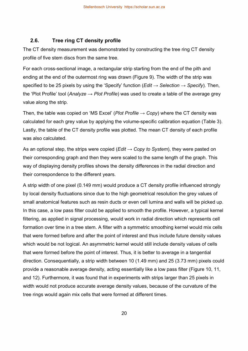
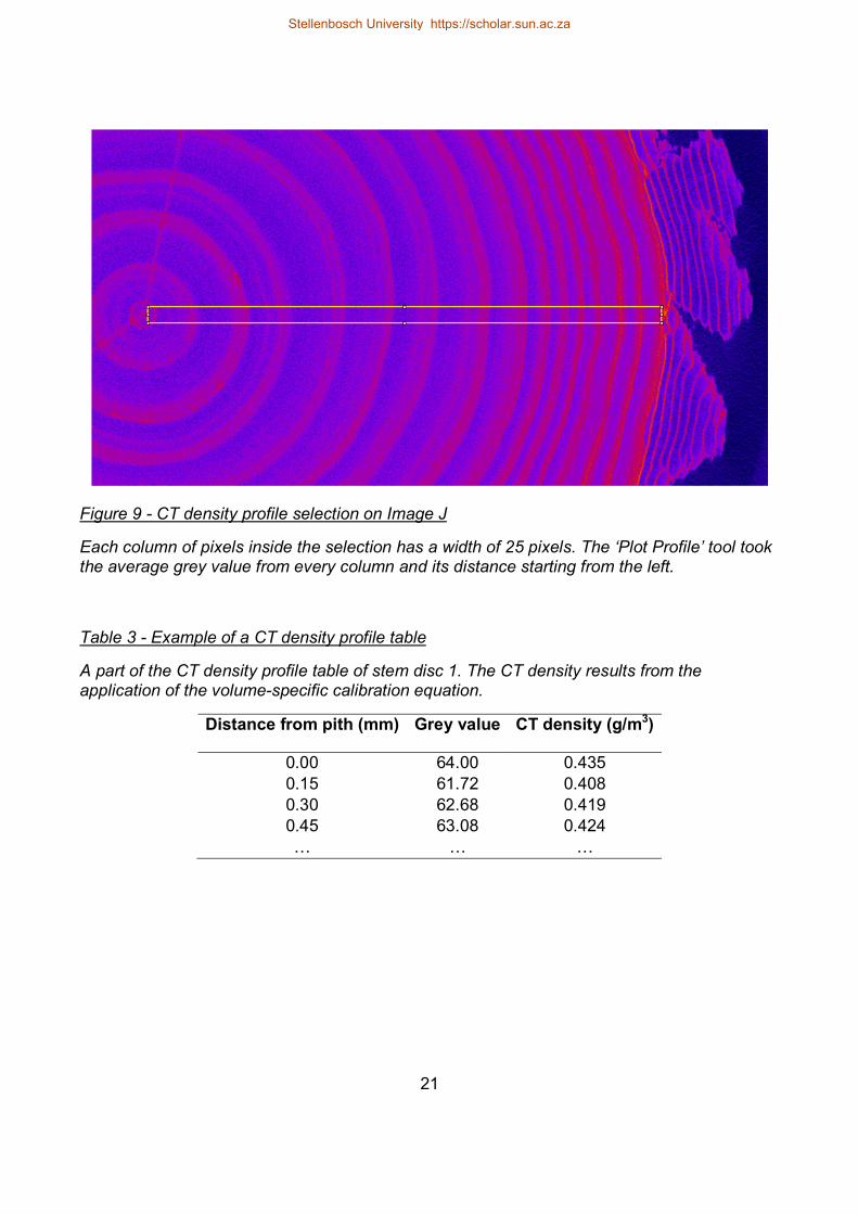
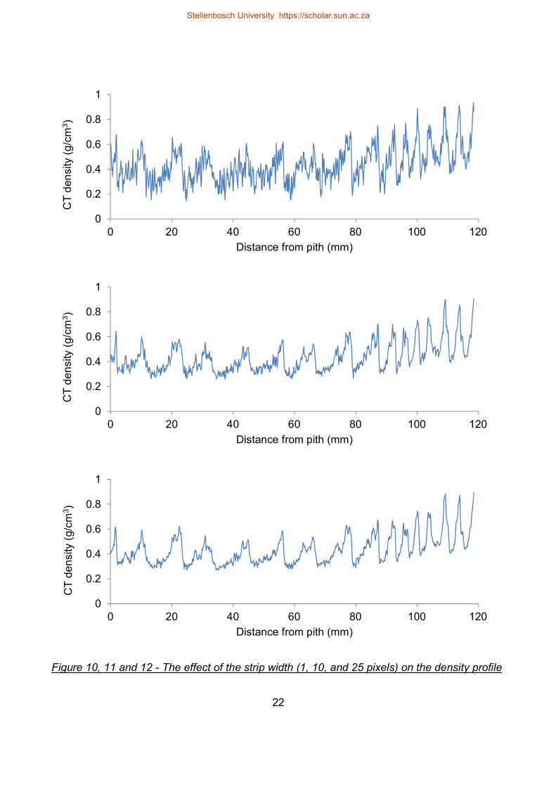
2.6. Tree ring CT density profile The CT density measurement was demonstrated by constructing the tree ring CT density profile of five stem discs from the same tree. For each cross-sectional image, a rectangular strip starting from the end of the pith and ending at the end of the outermost ring was drawn (Figure 9). The width of the strip was specified to be 25 pixels by using the ‘Specify’ function (Edit → Selection → Specify). Then, the ‘Plot Profile’ tool (Analyze → Plot Profile) was used to create a table of the average grey value along the strip. Then, the table was copied on ‘MS Excel’ (Plot Profile → Copy) where the CT density was calculated for each grey value by applying the volume-specific calibration equation (Table 3). Lastly, the table of the CT density profile was plotted. The mean CT density of each profile was also calculated. As an optional step, the strips were copied (Edit → Copy to System), they were pasted on their corresponding graph and then they were scaled to the same length of the graph. This way of displaying density profiles shows the density differences in the radial direction and their correspondence to the different years. A strip width of one pixel (0.149 mm) would produce a CT density profile influenced strongly by local density fluctuations since due to the high geometrical resolution the grey values of small anatomical features such as resin ducts or even cell lumina and walls will be picked up. In this case, a low pass filter could be applied to smooth the profile. However, a typical kernel filtering, as applied in signal processing, would work in radial direction which represents cell formation over time in a tree stem. A filter with a symmetric smoothing kernel would mix cells that were formed before and after the point of interest and thus include future density values which would be not logical. An asymmetric kernel would still include density values of cells that were formed before the point of interest. Thus, it is better to average in a tangential direction. Consequentially, a strip width between 10 (1.49 mm) and 25 (3.73 mm) pixels could provide a reasonable average density, acting essentially like a low pass filter (Figure 10, 11, and 12). Furthermore, it was found that in experiments with strips larger than 25 pixels in width would not produce accurate average density values, because of the curvature of the tree rings would again mix cells that were formed at different times.


21

Figure 9 - CT density profile selection on Image J Each column of pixels inside the selection has a width of 25 pixels. The ‘Plot Profile’ tool took the average grey value from every column and its distance starting from the left. Table 3 - Example of a CT density profile table A part of the CT density profile table of stem disc 1. The CT density results from the application of the volume-specific calibration equation.

Distance from pith (mm) Grey value CT density (g/m3) 0.00 64.00 0.435 0.15 61.72 0.408 0.30 62.68 0.419 0.45 63.08 0.424 … … …


22

Figure 10, 11 and 12 - The effect of the strip width (1, 10, and 25 pixels) on the density profile

00.20.40.60.8

1

0 20 40 60 80 100 120

CT de

nsity (

g/cm3 )

Distance from pith (mm)

00.20.40.60.8

1

0 20 40 60 80 100 120

CT de

nsity (

g/cm3 )


00.20.40.60.8

1

0 20 40 60 80 100 120

CT de

nsity (

g/cm3 )



23

2.7. Potential sources of CT density error 2.7.1. Homogeneity of phantom slices

Due to local density fluctuations or system noise, a large deviation in the grey value of the cross-sectional images (spacing of 1 mm) of a phantom slice could affect the regression and therefore the calibration equation. Thus, a large deviation in the grey value could be a potential source of CT density error. For this reason, the standard deviation of all the cross-sectional images of each phantom slice from five reconstructed volumes was calculated (15 slices × 5 reconstructed volumes = 75 slices).

2.7.2. Number of phantom slices Another potential source of CT density error could be the number of phantom slices used for the regression. An inadequate number of phantom slices would affect the reliability of the measured CT density. In order to determine the optimal number of phantom slices, regressions with 4, 6, 8, 10, and 12 phantom slices were performed for five reconstructed volumes (5 regressions with different number of slices × 5 reconstructed volumes = 25 regressions).


24

3. Results 3.1. Greyscale - density calibration

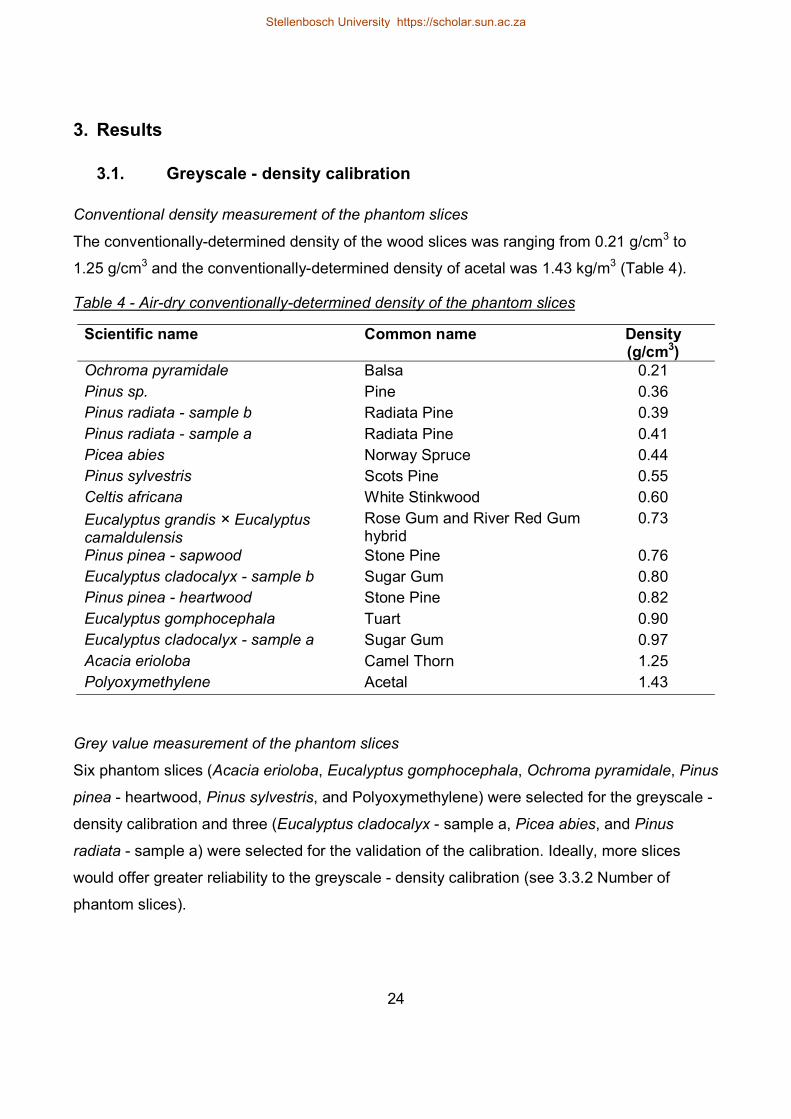
Conventional density measurement of the phantom slices The conventionally-determined density of the wood slices was ranging from 0.21 g/cm3 to 1.25 g/cm3 and the conventionally-determined density of acetal was 1.43 kg/m3 (Table 4). Table 4 - Air-dry conventionally-determined density of the phantom slices

Scientific name Common name Density (g/cm3)

Ochroma pyramidale Balsa 0.21 Pinus sp. Pine 0.36 Pinus radiata - sample b Radiata Pine 0.39 Pinus radiata - sample a Radiata Pine 0.41 Picea abies Norway Spruce 0.44 Pinus sylvestris Scots Pine 0.55 Celtis africana White Stinkwood 0.60 Eucalyptus grandis × Eucalyptus camaldulensis

Rose Gum and River Red Gum hybrid

0.73 Pinus pinea - sapwood Stone Pine 0.76 Eucalyptus cladocalyx - sample b Sugar Gum 0.80 Pinus pinea - heartwood Stone Pine 0.82 Eucalyptus gomphocephala Tuart 0.90 Eucalyptus cladocalyx - sample a Sugar Gum 0.97 Acacia erioloba Camel Thorn 1.25 Polyoxymethylene Acetal 1.43

Grey value measurement of the phantom slices Six phantom slices (Acacia erioloba, Eucalyptus gomphocephala, Ochroma pyramidale, Pinus pinea - heartwood, Pinus sylvestris, and Polyoxymethylene) were selected for the greyscale - density calibration and three (Eucalyptus cladocalyx - sample a, Picea abies, and Pinus radiata - sample a) were selected for the validation of the calibration. Ideally, more slices would offer greater reliability to the greyscale - density calibration (see 3.3.2 Number of phantom slices).


25

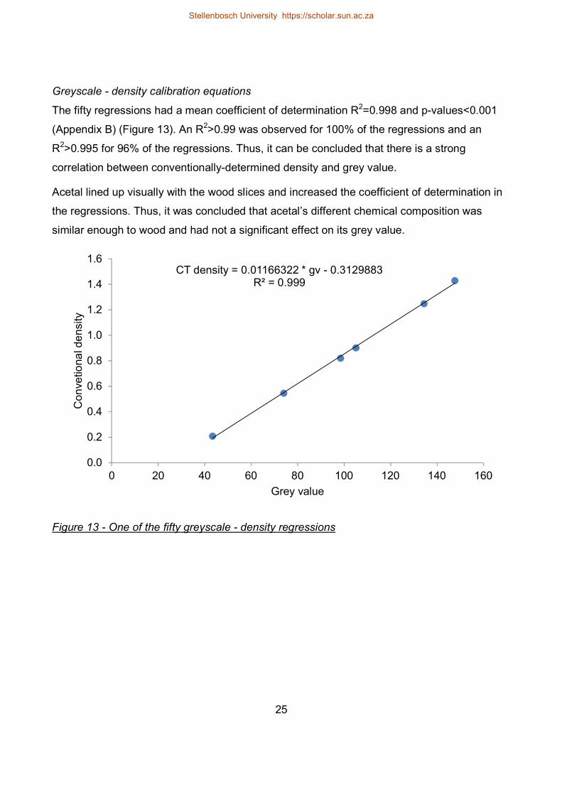
Greyscale - density calibration equations The fifty regressions had a mean coefficient of determination R2=0.998 and p-values<0.001 (Appendix B) (Figure 13). An R2>0.99 was observed for 100% of the regressions and an R2>0.995 for 96% of the regressions. Thus, it can be concluded that there is a strong correlation between conventionally-determined density and grey value. Acetal lined up visually with the wood slices and increased the coefficient of determination in the regressions. Thus, it was concluded that acetal’s different chemical composition was similar enough to wood and had not a significant effect on its grey value.

Figure 13 - One of the fifty greyscale - density regressions

CT density = 0.01166322 * gv - 0.3129883R² = 0.999

0.00.20.40.60.81.01.21.41.6

0 20 40 60 80 100 120 140 160

Conve

tional d

ensity

Grey value


26

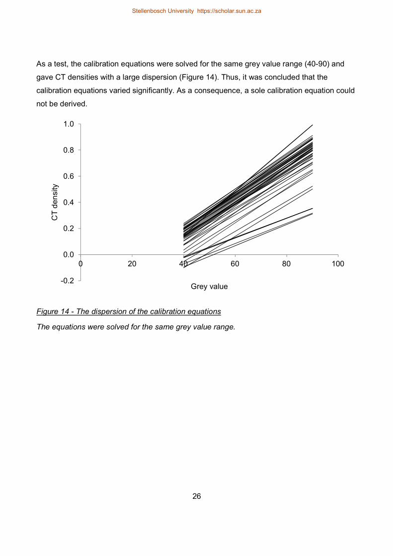
As a test, the calibration equations were solved for the same grey value range (40-90) and gave CT densities with a large dispersion (Figure 14). Thus, it was concluded that the calibration equations varied significantly. As a consequence, a sole calibration equation could not be derived.

Figure 14 - The dispersion of the calibration equations The equations were solved for the same grey value range.

-0.2

0.0

0.2

0.4

0.6

0.8

1.0

0 20 40 60 80 100

CT de

nsity

Grey value


27

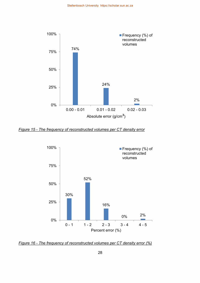
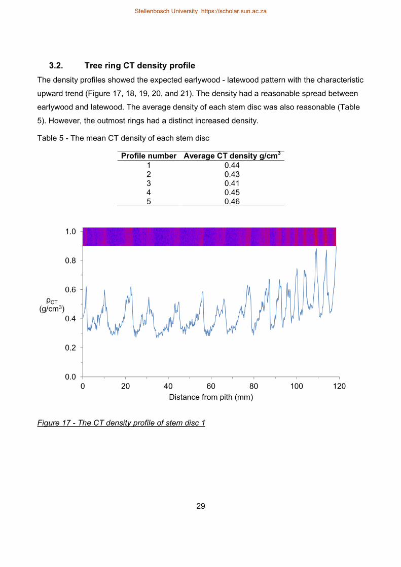
Validation of the greyscale - density calibration equations The absolute CT density error of the reconstructed volumes was ranging from 0.002 - 0.026 g/cm3 and had a mean of 0.008 g/cm3 (σ=0.004). Specifically, the absolute CT density error was smaller than 0.01 g/cm3 for 74% (n=37) of the reconstructed volumes, it was ranging between 0.01 and 0.02 g/cm3 for 24% (n=12) of the volumes and it was ranging from 0.02 to 0.03 g/cm3 for 2% (n=1) of the volumes (Figure 15). The percent CT density error of the reconstructed volumes was ranging from 0.4% - 4.4% and had a mean of 1.4% (σ=0.7). Specifically, the percent CT density error was smaller than 1% for 30% (n=15) of the volumes, it was ranging between 1 and 2% for 52% (n=26) of the volumes, it was ranging between 2 and 3% for 16% (n=8) of the volumes and it was larger than 3% for 2% (n=1) of the volumes (Figure 16).


28

Figure 15 - The frequency of reconstructed volumes per CT density error

Figure 16 - The frequency of reconstructed volumes per CT density error (%)

74%

24%

2%0%

25%

50%

75%

100%

0.00 - 0.01 0.01 - 0.02 0.02 - 0.03Absolute error (g/cm³)

Frequency (%) ofreconstructedvolumes

30%

52%

16%

0% 2%0%

25%

50%

75%

100%

0 - 1 1 - 2 2 - 3 3 - 4 4 - 5Percent error (%)

Frequency (%) ofreconstructedvolumes


29

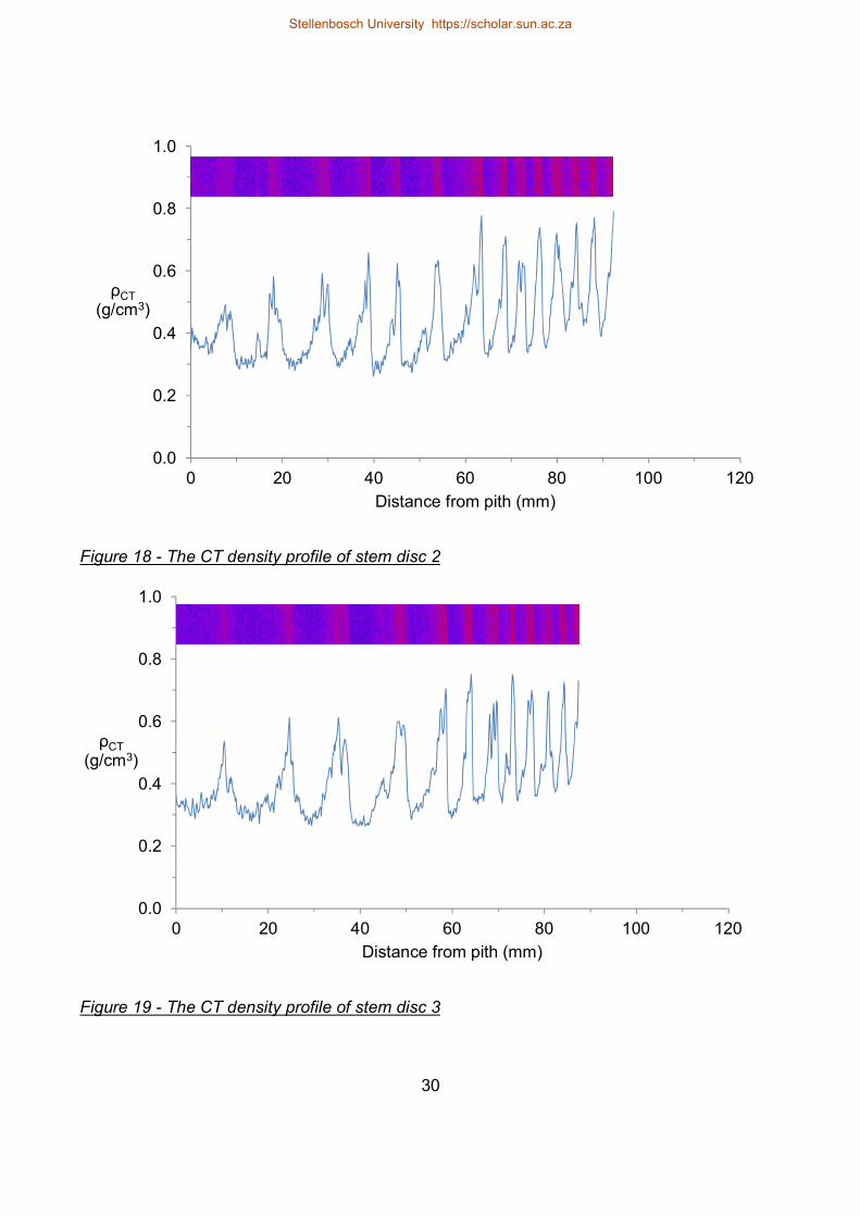
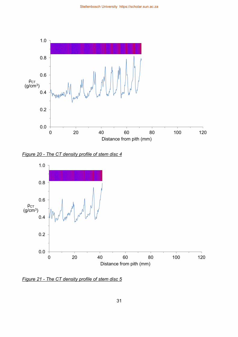
3.2. Tree ring CT density profile The density profiles showed the expected earlywood - latewood pattern with the characteristic upward trend (Figure 17, 18, 19, 20, and 21). The density had a reasonable spread between earlywood and latewood. The average density of each stem disc was also reasonable (Table 5). However, the outmost rings had a distinct increased density. Table 5 - The mean CT density of each stem disc

Profile number Average CT density g/cm3 1 0.44 2 0.43 3 0.41 4 0.45 5 0.46

Figure 17 - The CT density profile of stem disc 1

0.0

0.2

0.4

0.6

0.8

1.0

0 20 40 60 80 100 120

ρCT(g/cm3)



30



0.0

0.2

0.4

0.6

0.8

1.0

0 20 40 60 80 100 120

ρCT(g/cm3)


0.0

0.2

0.4

0.6

0.8

1.0

0 20 40 60 80 100 120

ρCT(g/cm3)



31



0.0

0.2

0.4

0.6

0.8

1.0

0 20 40 60 80 100 120

ρCT(g/cm3)


0.0

0.2

0.4

0.6

0.8

1.0

0 20 40 60 80 100 120

ρCT(g/cm3)



32

3.3. Potential sources of CT density error 3.3.1. Homogeneity of phantom slices

The standard deviation in the grey value of the cross-sectional images was s<1 for 95% of the phantom slices (71 out of 75 slices). The 100% of the slices had a standard deviation s<1.5. Therefore, the deviation in the grey value of the cross-sectional images of a phantom slice has a small or negligible effect on the conventional density - grey value regression.

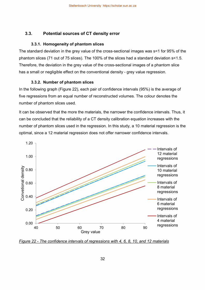
3.3.2. Number of phantom slices In the following graph (Figure 22), each pair of confidence intervals (95%) is the average of five regressions from an equal number of reconstructed volumes. The colour denotes the number of phantom slices used. It can be observed that the more the materials, the narrower the confidence intervals. Thus, it can be concluded that the reliability of a CT density calibration equation increases with the number of phantom slices used in the regression. In this study, a 10 material regression is the optimal, since a 12 material regression does not offer narrower confidence intervals.

Figure 22 - The confidence intervals of regressions with 4, 6, 8, 10, and 12 materials

0.00

0.20

0.40

0.60

0.80

1.00

1.20

40 50 60 70 80 90

Conve

tional d

ensity

Grey value

Intervals of12 materialregressionsIntervals of10 materialregressionsIntervals of8 materialregressionsIntervals of6 materialregressionsIntervals of4 materialregressions


33

4. Discussion 4.1. Accuracy and repeatability of the greyscale - density calibration

4.1.1. CT density error It can be concluded that the greyscale - density calibration was achieved with a small amount of error and a high repeatability because:

(i) The absolute CT density error of the reconstructed volumes was ranging from 0.002 - 0.026 g/cm3 with a mean of 0.008 g/cm3 (σ=0.004).

(ii) The percent CT density error of the reconstructed volumes was ranging from 0.4% - 4.4% with a mean of 1.4% (σ=0.7).

(iii) For 98% of the reconstructed volumes, the absolute CT density error was smaller than 0.02 g/cm3 and the percent CT density error was smaller than 3% (Figure 15 and 16).

Likewise, it can be concluded that the creation of the tree ring CT density profiles (Figure 17, 18, 19, 20 and 21) was also achieved because:

(i) The reconstructed volume that was used for the tree ring CT density profiles had an absolute CT density error of 0.003 g/cm3 which indicates a small amount of error in other CT density values.

(ii) The observed air-dry CT density is consistent with the reported air-dry density of P. radiata. The mean CT density of the profiles was ranging from 0.41 to 0.46 g/cm3 while the reported density of P. radiata was about 0.48 g/cm3 in 10 to 20 year old trees (Forest Products Commission Western Australia, 2015).

However, the density of the outmost rings was rather high, which can be attributed to beam hardening or to an increased content of resin in that sapwood region.

4.1.2. Homogeneity of phantom slices The grey value of the cross-sectional images did not deviate significantly (s<1) for 95% of the measured phantom slices (71 out of 75 slices). Thus, any inhomogeneity, due to the earlywood and latewood pattern or due to system noise, had a small or negligible effect on the deviation of the grey value and therefore to the greyscale - density calibration.


34

4.1.3. Number of phantom slices Six phantoms slices were used for the greyscale - density calibration and three for the validation of the calibration. It was observed that a higher number of phantom slices increase the reliability of the calibration equations. Therefore, greyscale - density calibrations with more phantom slices could have possibly reduced the CT density error.

4.1.4. Chemical composition of phantom slices The measured grey value of a phantom slice is defined among others by its chemical composition. For this reason, the chemical composition of the materials of a phantom should be similar to the objects of interest (Phillips & Lannutti, 1997; Stoel et al., 2008). The difference in density between species is not an effect of different chemical composition but it depends on the proportion of the cell wall material and air in dry wood. Thus, air-dry wood density can range from very light wood such as Ochroma pyramidale (150 kg/m3) to very dense wood such as Guaiacum officinale (1300 kg/m3). The cell wall consists from cellulose (C6H10O5), hemicellulose, lignin (C9H10O2, C10H12O3, C11H14O4) and pectin (C6H10O7) and their density is ranging around 1.5 gr/cm3 (Kellogg & Wangaard, 1969; Gibson, 2012). Wood, as a porous material, also contains air (N2, O2, Ar and CO2) (0.001225 g/cm3) and water (H2O) (1 g/cm3). Thus, it is critical for precise CT density measurements to dry the imaging phantom and the examined wood samples to constant moisture content (Cleaveland, 1983). Phiri (2013) showed how differences in drying temperature can affect the equilibrium weight of Eucalyptus. In X-ray densitometry, the air-dried density (around 12%) is common (Bouriaud et al., 2005; Taylor, 2006; Tomazello et al., 2008; Freyburger et al., 2009; De Ridder et al., 2011). The moisture content of the stem discs and the imaging phantom materials was not measured again after the scans. Thus, the CT density error can possibly be partially attributed to the control of the moisture content. Furthermore, wood contain various extractives which are organic and inorganic, non-structural materials that contribute to density substantially, especially in heartwood (Cown & Harris, 1991). In particular, conifers are known to have high resin contents and can additionally form pitch pockets (Seifert et al. 2010b). In order for the scanned materials to have similar chemical composition, resins can be removed by alcohol (Zamudio et al., 2002) or an alcohol-benzene solution (Cleaveland, 1983). It is possible that such differences in chemical composition can also be considered partially responsible for the CT density error. In


35

this point, the densities of CT-scanned samples are not comparable with results from 2D X-ray densitometry, where typically the extractives are extracted before X-ray exposure. Regarding acetal ((CH2O)n), it can be concluded that its different chemical composition had not a significant effect on its grey value, since it lined up visually with the other materials and it increased the coefficient of determination of the regressions. This was expected since acetal is traditionally used as a homogeneous calibration material for 2D X-ray densitometry (e.g. Hoag 1988)

4.1.5. Stability of the calibrations In studies with medical CT scanners, a single calibration equation is reported to be sufficient, provided the scanner settings are kept the same (Lindgren, 1991a; Taylor, 2006; Freyburger et al., 2009). In contrast, in this study, each reconstructed volume needed a specific greyscale - density calibration equation. This can be attributed to the automatic assignment of the grey values (grey value scaling) by the CT scanner, with black voxels representing air as the material with the lowest density in the scan and white voxels representing poster putty as the material with the highest density in the scan. Specifically, it could be observed by visual inspection of the images that some volumes were brighter or darker than others. Therefore, the shift of the grey values from volume to volume contributed to differences of the calibration equations. It has to be noted, though, that the shift of the grey values did not affect the CT density error. Specifically, in seven volumes, the whitest voxels belonged to (metallic) staples. Although, the assignment of the grey values was different, the CT density error of these volumes was about the same with the rest. To sum up these results, it can be stated that it is necessary to scan calibration phantoms with every scan, if a plausible and comparable density should be determined.

4.2. Spatial accuracy A higher spatial resolution increases the structural detail of a reconstructed object. A higher resolution can be achieved by reducing the distance between the X-ray tube and the object so that and the projection on the detector is covered by more detector elements. Thus, it was attempted to minimize this distance as much as possible. The distance that was chosen as optimal was the distance that the projection of the larger stack of stem discs was marginally


36

fitting on the X-ray detector. This distance resulted in a spatial resolution of approximately 150 μm/voxel or 6.7 voxels/mm when scanning a stack of discs. In comparison with a similar study, De Ridder et al., (2011) scanned wood cores with a spatial resolution of 50 μm/voxel. In X-ray radiography, the spatial resolution (digitized X-ray film negatives) is larger and each ring can be divided in 100 segments in order to provide an equal number of density values (Cleaveland, 1983; Bouriaud et al., 2005; Rathgeber et al., 2006). However the obtainable resolution is clearly determined by sample size which in this study was considerably larger than in the other mentioned studies so that a trade-off between sample size and spatial resolution was evident.

4.3. Outlook on future work The requirement for accurately-determined CT density and the requirement for comparison of results from different studies that involve CT densitometry lead inevitably to the standardization of the CT densitometry of wood. Thus, future work that targets this standardization could focus on:

i) The fabrication and use of homogeneous phantom compartments from cellulose of different packing. An alternative to solid wood phantoms can be the use of wood pulp phantoms from wood pulp of various densities. This is similar to the calibration wedges from wood pulp that have been used in X-ray radiography (Cleaveland, 1983). Furthermore, if the chemical composition of a wood pulp phantom was to be known, then the density could be calculated in principle and it could be used as a prediction for the CT density.

ii) The automatic volume-based grey value measurement of phantom slices in order to increase the accuracy and repeatability of the grey value measurement process. Additionally, the automatic measurement could decrease the required time for measuring a phantom slice and thus it could process a larger number of phantoms slices which would increase the accuracy of the calibration and the accuracy of the validation. The automatic measurement possible through the fabrication of the proper phantom and the use of the proper software (Stoel et al., 2008).

iii) The effect of various factors such as voltage, amperage and effective atomic number on the greyscale - density calibration.


37

iv) The simultaneous scan of imaging phantom and wood samples and its effect on the greyscale - density calibration due to artefacts such as beam hardening.

v) The further investigation of the stability of the calibration procedure with perspective the derivation of a single calibration equation.

With these proposed future improvements, X-ray based microdensitometry could enfold its full potential with regards to the application in wood and forest science.


38

5. Conclusions It was successfully demonstrated that an industrial cone-beam CT scanner can be used for wood microdensitometry and, furthermore, for the creation of tree ring CT density profiles. The absolute CT density error of the reconstructed volumes was ranging from 0.002 - 0.026 g/cm3 with a mean of 0.008 g/cm3 (σ=0.004) (Figure 15). The percent CT density error of the reconstructed volumes was ranging from 0.4% - 4.4% with a mean of 1.4% (σ=0.7) (Figure 16). The CT density error can possibly be attributed to:

(i) The small number of phantom slices. Specifically, six phantoms slices were used for the greyscale - density calibration and three for the validation of the calibration.

(ii) Differences in the chemical composition of the phantom slices and the wood samples. These are the moisture content, resins and various other extractives.

The CT density error cannot be attributed to the inhomogeneity of wood. Acetal can be used as an extra reference material in the imaging phantom, since its different chemical composition in relation to wood does not affect its grey value. Lastly, it is necessary to scan calibration phantoms with every scan, in order to achieve a plausible and comparable density.


39

6. Reference List Beer, A. (1852). Bestimmung der Absorption des rothen Lichts in farbigen Flüssigkeiten

(Determination of the absorption of red light in colored liquids). Annalen der Physik und Chemie, 86, 78-88.

Bouriaud, O., Leban, J. M., Bert, D., & Deleuze, C. (2005). Intra-annual variations in climate influence growth and wood density of Norway spruce. 25(6), 651-660. doi:10.1093/treephys/25.6.651

Briffa, K. R., Jones, P. D., Osborn, T. J., Schweingruber, F. H., Shiyatov, S. G., & Vaganov, E. A. (2002). Tree-ring width and density data around the Northern Hemisphere: Part 1, local and regional climate signals. The Holocene, 12, 737-757. doi:10.1191/0959683602hl587rp

Briffa, K. R., Jones, P. D., Schweingruber, F. H., & Osborn, T. J. (1998). Influence of volcanic eruptions on Northern hemisphere summer temperatures over the past 600 years. Nature, 393, 450-455.

Briffa, K. R., Jones, P. D., Schweingruber, F. H., Shiyatov, S. G., & Cook, E. R. (1995). Unusual twentieth-century summer warmth in a 1000-year temperature record from Siberia. Nature, 376, 156-159.

Bucur, V. (2003a). Non-destructive Characterization and Imaging of Wood (1st ed.). Berlin: Springer Veerlag Berlin Heidelberg New York.

Bucur, V. (2003b). Ultrasonic imaging of wood structure. Proceedings of the World Congress on Ultrasonics. Paris: Société française d'acoustique.

Chave, J., Muller-Landau, H. C., Baker, T. R., Easdale, T. A., ter Steege, H., & Webb, C. O. (2006). Regional and phylogenetic variation of wood density across 2456 neotropical tree species. Ecological Applications, 16(6), 2356-2367.

Cleaveland, M. K. (1983). X-Ray Densitometric Measurement of Climatic Influence on the Intra-Annual Characteristics of Southwestern Semiarid Conifer Tree Rings. PhD Thesis: University of Arizona.

Cleaveland, M. K. (1986). Climatic Response of Densitometric Properties in Semiarid Site Tree Rings. Tree-Ring Bulletin, 46, 13-29.


40

Cook, E. R., & Kairiukstis, L. A. (1990). Methods of Dendrochronology. Netherlands: Springer. doi:10.1007/978-94-015-7879-0

Cormack, A. M. (1963). Representation of a function by its line integrals, with some radiological applications. Journal of applied physics, 34(9), 2722-2727.

Cown, D. J. (1999). Wood Characteristics of New Zealand Radiata pine and Douglas fir: Suitability for processing (2nd ed.). Rotorua, New Zealand: New Zealand Forestry Corporation Limited.

Cown, D. J., & Ball, R. D. (2001). Wood densitometry of ten Pinus radiata families at seven contrasting sites: Influence of tree age, site and genotype. New Zealand Journal of Forest Science, 31(1), 88-100.

Cown, D. J., & Harris, J. M. (1991). Basic Wood Properties. In J. A. Kinimonth, & L. J. Whitehouse, Properties and uses of New Zealand Radiata pine (Vol. 1, pp. 6.1-6.28). Rotorua, New Zealand: New Zealand Ministry of Forestry, Forest Reasearch Institute, with assistance from the New Zealand Lottery Grants Board.

Cown, D. J., & McConchie, D. L. (1980). Wood property variations in an old-crop stand of radiata pine. New Zealand Journal of Forestry Science, 10(3), 508-520.

Cown, D. J., McConchie, D. L., & Young, G. D. (1991). Radiata Pine: Wood Properties Survey. Rotorua, New Zealand: Forest Reasearch Institute.

D’Arrigo, R. D., Jacoby, G. C., & Free, R. M. (1992). Tree ring width and maximum latewood density at the North American tree line: parameters of climate change. Canadian Journal of Forest Research, 22, 1290-1296.

De Ridder, M., Van den Bulcke, J., Vansteenkiste, D., Van Loo, D., Dierick, M., Masschaele, B., . . . Van Acker, J. (2011). High-resolution proxies for wood density variations in Terminalia superba. Annals of Botany, 107(2), 293-302. doi:10.1093/aob/mcq224

Decoux, V., Varcin, É., & Leban, J.-M. (2004). Relationships between the intra-ring wood density assessed by X-ray densitometry and optical anatomical measurements in conifers. Consequences for the cell wall apparent density determination. Annals of Forest Science, 61, 251-262. doi:10.1051/forest:2004018


41

du Plessis, A., Meincken, M., & S. T. (2013). Quantitative Determination of Density and Mass of Polymeric Materials Using Microfocus Computed Tomography. Journal of Nondestructive Evaluation, 32, 413–417.

Espinoza, G. R., Hernández, R., Condal, A., Verret, D., & Beauregard, R. (2005). Exploration of the Physical Properties of Internal Characteristics of Sugar Maple Logs and Relationships with CT Images. Wood and Fiber Science, 37(4), 591-604.

Fischer, P. M. (2011). δ13C as indicator of soil water availability and drought stress in Pinus radiata stands in South Africa. Stellenbosch: Stellenbosch University.

Forest Products Commission Western Australia. (2015). Forest Products Commission Western Australia. Retrieved 12 10, 2015, from http://www.fpc.wa.gov.au/content_migration/plantations/species/plantations/radiata_pine.aspx

Freyburger, C., Longuetaud, F., Mothe, F., Constant, T., & Leban, J.-M. (2009). Measuring wood density by means of X-ray computer tomography. Annals of Forest Science, 66(8). doi:<10.1051/forest/2009071>

Fritts, H. (1976). Tree Rings and Climate. London: Academic Press Inc. Gibson, L. J. (2012). The hierarchical structure and mechanics of plant materials. Journal of

the Royal Society. Guilley, É., Hervé, J.-C., Huber, F., & Nepveu, G. (1999). Modelling variability of within-ring

density components in Quercus petraea Liebl. with mixed-effect models and simulating the influence of contrasting silvicultures on wood density. Annals of Forest Science, 56, 449-458.

Hoag, M. L. (1988). Measurement of Within-Tree Density Variations in Douglas-fir (Pseudotsuga menzeisii (Mirb.) Franco Using Direct Scanning X-ray Techniques. MSc Thesis: Oregon State University p.96.

Hou, Z. Q., Wei, Q., & Zhang, S. Y. (2007). Predicting density of green logs using the computed tomography technique. Forest Products Journal, 59(5), 53-57.

Hounsfield, G. N. (1973). Computerized transverse axial scanning (tomography): Part 1. Description of system. The British journal of radiology, 46(552), 1016-1022.


42

Hughes, M. K., Schweingruber, F. H., Cartwright, D., & Kelly, P. M. (1984). July-August temperature at Edinburgh between 1721 and 1975 from tree-ring density and width data. Nature, 308, 341-344.

Kalender, W. A. (2000). Computed Tomography. MCD Verlag. Kellogg, R. M., & Wangaard, F. F. (1969). Variation in The Cell-Wall Density of Wood. Wood

and Fiber Science, 1. Klisz, M. (2013). Genetic control of wood density, tracheid dimension and annual ring traits -

an analysis of genetic and phenotypic correlation in European larch. Annals of Warsaw University of Life Sciences - SGGW, 83, 37-41.

Knapic, S., Louzada, J. L., Leal, S., & Pereira, H. (2007). Radial variation of wood density components and ring width in cork oak trees. Annals of Forest Science, 64(2), 211-218. doi:10.1051/forest:2006105

Koubaa, A., Zhang, S. T., & Makni, S. (2002). Defining the transition from earlywood to latewood in black spruce based on intra-ring. Annals of Forest Science, 59(5-6), 511-518. doi:10.1051/forest:2002035

Laufenberg, T. L. (1986). Using gamma radiation to measure density gradients in reconstituted wood products. Forest Products Journal, 36(2), 59-62.

Lindgren, L. O. (1991a). Medical CAT-scanning X-ray absorption coefficients, CT-numbers and their relation to wood density. Wood Science Technology, 25, 341-349.

Lindgren, L. O. (1991b). The accuracy of medical CAT-scan images for non-destructive density measurements in small volume elements within solid wood. Wood Science Technology, 25, 425-432.

Macedo, A., Vaz, C. M., Pereira, J. C., Naime, J. M., Cruvinel, P. E., & Crestana, S. (2002). Wood density determination by X- and gamma-ray tomography. Holzforschung, 56(5), 535-540.

Magalhães, T. M., & Seifert, T. (2015a). Estimation of tree biomass, carbon stocks and error propagation in Mecrusse woodlands. Open Journal of Forestry, 5, 471-488.


43

Magalhães, T. M., & Seifert, T. (2015b). Tree component biomass expansion factors and root-to-shoot ratio of Lebombo ironwood: measurement uncertainty. Carbon Balance and Management, 10(9). doi:DOI: 10.1186/s13021-015-0019-4

Mäkipää, R., & Linkosalo, T. (2011). A Non-Destructive Field Method for Measuring Wood Density of Decaying Logs. Silva Fennica, 45(5), 1135–1142. Retrieved from http://www.metla.fi/silvafennica/full/sf45/sf4551135.pdf

Mull, R. T. (1984). Mass Estimates by Computed Tomography: Physical Density from CT Numbers. American Journal of Roentgenology, 143, 1101-1104.

Nikolova, P. S., Blaschke, H., Matyssek, R., Pretzsch, H., & Seifert, T. (2009). Combined application of computer tomography and light microscopy for analysis of conductive xylem area in coarse roots of European beech and Norway spruce. European Journal of Forest Research, 128, 145-153. doi:10.1007/s10342-008-0211-0

Nocetti, Rozenberg, Chaix, & Macchioni. (2011). Provenance effect on the ring structure of teak (Tectona grandis L.f.) wood by X-ray microdensitometry. Annals of Forest Science, 68(8), 1375-1383. doi:10.1007/s13595-011-0145-4

Odhiambo, B. O. (2015). The effect of fire damage on the growth and survival mechanisms of selected native and commercial trees in South Africa. PhD thesis at the Department of Forest and Wood Science. Stellenbosch University, South Africa.

Parker, M. L., & Meleskie, K. R. (1970). Preparation of X-ray negatives of tree-ring specimens for dendrochronological analysis. ree-Ring Bulletin, 30, 11-22.

Phillips, D. H., & Lannutti, J. J. (1997). Measuring physical density with X-ray computed tomography. NDT&E International, 30(6), 339-350.

Phillips, E. W. (1960). The beta ray method of determing the density of wood and the proportion of summerwood. Journal of the Institute of Wood Science, 5-8.

Phiri, D. (2013). Biomass Modelling of Selected Drought Tolerant Eucalypt Species in South Africa. MSc thesis at the Department of Forest and Wood Science. Stellenbosch University, South Africa.


44

Phiri, D., Ackerman, P. A., Wessels, B., Johansson, M., Säll, H., Lundqvist, S.-O., . . . Seifert, T. (2015). Biomass Equations for Selected Drought Tolerant Eucalypts in South Africa. Southern Forests, 3, 1-8. doi:10.2989/20702620.2015.1055542

Polge, H. (1966). Établissement des courbes de variation de la densité du bois par exploration densitométrique de radiographies d'échantillons prélevés à la tarière sur des arbres vivants : applications dans les domaines Technologique et Physiologique. Annals of Forest Science, 23(1), 1-206. doi:10.1051/forest/19660101

Polge, H. (1970). The use of X-ray densitometric methods in dendrochronology. Tree-ring bulletin, 30(1), 1-10.

Rathgeber, C. B., Decoux, V., & Leban, J.-M. (2006). Linking intra-tree-ring wood density variations and tracheid anatomical characteristics in Douglas fir (Pseudotsuga menziesii (Mirb.) Franco). Annals of Forest Science, 63(7), 699-706. doi:10.1051/forest:2006050

Rautkari, L., Kamke, F. A., & Hughes, M. (2010). Potential error in density profile measurements for wood composites. European Journal of Wood and Wood Products, 69(1), 167-169. doi:10.1007/s00107-010-0419-9

Revel, R. (1982). The use of scanning electron microscopy as a tool in dendrochronology. Tree-Ring Bulletin, 42, 57-64.

Rinn, F. (2012). Basics of typical resistance-drilling profiles. Western Arborist, 30-36. Rinn, F., Schweingruber, F. H., & Schär, E. (1996). RESISTOGRAPH and X-ray Density

Charts of Wood Comparative Evaluation of Drill Resistance Profiles and X-ray Density Charts of Different Wood Species. Holzforschung, 50(4), 303-311.

Robinson, A. P., & Hamann, J. D. (2011). Forest Analytics with R. New York, Dordrecht, Heidelberg, London: Springer Science+Business Media. doi:10.1007/978-1-4419-7762-5

Schinker, M. G., Hansen, N., & Spiecker, H. (2003). High-Frequency Densitometry – A New Method for the Rapid Evaluation of Wood Density Variations. IAWA Journal, 24(3), 231-239.


45

Schweingruber, F. H. (1988). Tree Rings: Basics and Applications of Dendrochronology. (1, Ed.) Dordrecht: Springer Netherlands. doi:10.1007/978-94-009-1273-1

Schweingruber, F. H., & Kienast, F. (1986). Dendroecological Studies in the Front Range, Colorado, U.S.A. Arctic and Alpine Research, 18(3), 277-288. Retrieved from http://www.jstor.org/stable/1550885

Schweingruber, F., Fritts, H., Bräker, O., Drew, L., & Schär, E. (1978). The X-Ray Technique as Applied to Dendroclimatology. Tree-Ring Bulletin, 38, 61-91.

Seifert, T., & Seifert, S. (2014). Modelling and simulation of tree biomass. In T. Seifert (Ed.), Bioenergy from Wood: Sustainable Production in the Tropics (1 ed., pp. 42-65). Netherlands: Springer.

Seifert, T., Breibeck, J., Seifert, S., & Biber, P. (2010b). Resin pocket occurrence in Norway spruce depending on tree and climate variables. Forest Ecology and Management, 260, 302–312.

Seifert, T., Nickel, M., & Pretzsch, H. (2010). Analysing the long-term effects of artificial pruning of wild cherry by computer tomography. Trees, 24, 797-808. doi:10.1007/s00468-010-0450-9

Steppe, K., Cnudde, V., Girard, C., Lemeur, R., Cnudde, J.-P., & Jacobs, P. (2004). Use of X-ray computed microtomography for non-invasive determination of wood anatomical characteristics. Journal of Structural Biology, 148, 11-21. doi:10.1016/j.jsb.2004.05.001

Stoel, B. C., Bode, F., Rames, A., Soliman, S., Reiber, J. H., & Stolk, J. (2008, 12 15). Quality Control in Longitudinal Studies with Computed Tomographic Densitometry of the Lungs. Proceedings of the American Thoracic Society, 5(9), 929-933.

Taylor, A. J. (2006). Wood density determination in Picea sitchensis using computerised tomography; how do density measurements compare with measurements of pilodyn pin penetration (Honours Project). Bangor: The University of Wales.

Tomazello, M., Brazolin, S., Chagas, M. P., Oliveira, J. T., Ballarin, A. W., & Benjamin, C. A. (2008). Application of X-Ray Technique in Nondestructive Evaluation of Eucalypt Wood. Maderas: Ciencia y tecnología, 10(2), 139-149.


46

Vaganov, E. A., Hughes, M. K., & Shashkin, A. V. (2006). Growth Dynamics of Conifer Tree Rings. Berlin Heidelberg: Springer-Verlag.

Vahey, D. W., Zhu, J. Y., & Scott, C. T. (2007). Wood density and anatomical properties in suppressed-growth trees: Comparison of two methods. Wood and Fiber Science, 39(3), 462-471.

Warton, D., Wright, I., Falster, D., & Westoby, M. (2006). Bivariate line-fitting methods for allometry. Biological reviews of the Cambridge Philosophical Society, 81(2), 259–291.

Wessels, C. B., Malan, F. S., Seifert, T., Louw, J. H., & Rypstra, T. (2015). The prediction of the flexural lumber properties from standing South African grown Pinus patula trees. European Journal of Forest Research, 134(1), 1-18.

Zamudio, F., Baettyg, R., Vergara, A., Guerra, F., & Rozenberg, P. (2002). Genetic trends in wood density and radial growth with cambial age in a radiata pine progeny test. Annals of Forest Science, 59(5-6), 541-549. doi:10.1051/forest:2002039

zu Castell, W., Schrödl, S., & Seifert, T. (2005). Volume Interpolation of CT Images from Tree Trunks. Plant Biology, 7, 737-744.


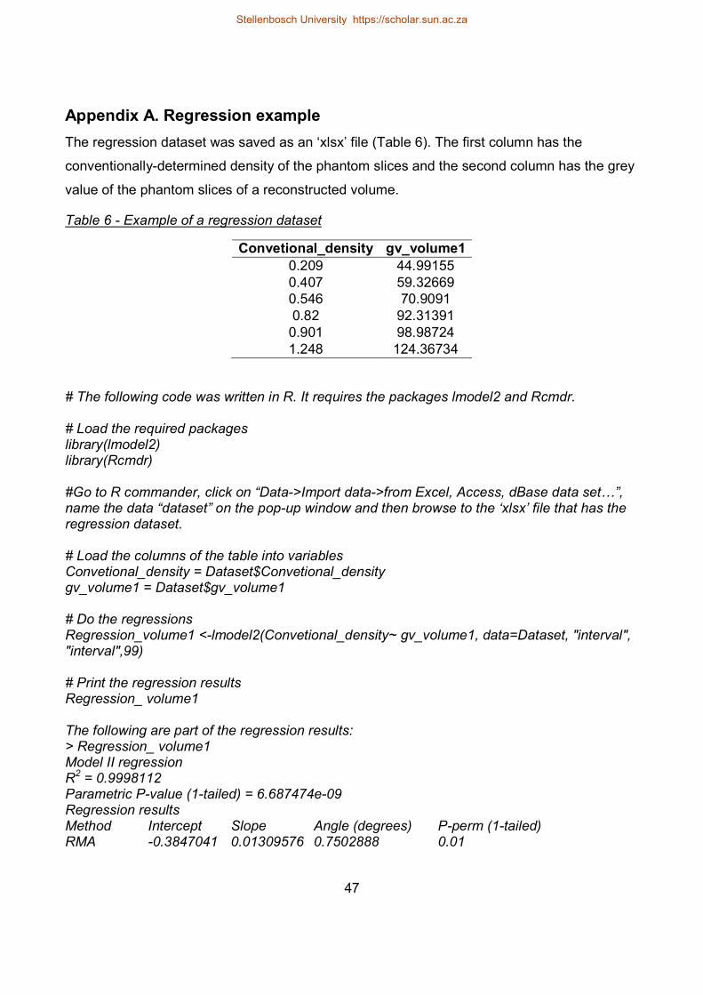
47

Appendix A. Regression example The regression dataset was saved as an ‘xlsx’ file (Table 6). The first column has the conventionally-determined density of the phantom slices and the second column has the grey value of the phantom slices of a reconstructed volume. Table 6 - Example of a regression dataset

Convetional_density gv_volume1 0.209 44.99155 0.407 59.32669 0.546 70.9091 0.82 92.31391

0.901 98.98724 1.248 124.36734

# The following code was written in R. It requires the packages lmodel2 and Rcmdr. # Load the required packages library(lmodel2) library(Rcmdr) #Go to R commander, click on “Data->Import data->from Excel, Access, dBase data set…”, name the data “dataset” on the pop-up window and then browse to the ‘xlsx’ file that has the regression dataset. # Load the columns of the table into variables Convetional_density = Dataset$Convetional_density gv_volume1 = Dataset$gv_volume1 # Do the regressions Regression_volume1 <-lmodel2(Convetional_density~ gv_volume1, data=Dataset, "interval", "interval",99) # Print the regression results Regression_ volume1 The following are part of the regression results: > Regression_ volume1 Model II regression R2 = 0.9998112 Parametric P-value (1-tailed) = 6.687474e-09 Regression results Method Intercept Slope Angle (degrees) P-perm (1-tailed) RMA -0.3847041 0.01309576 0.7502888 0.01


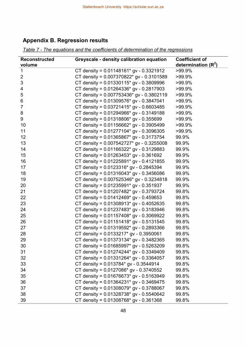
48

Appendix B. Regression results Table 7 - The equations and the coefficients of determination of the regressions

Reconstructed volume

Greyscale - density calibration equation Coefficient of determination (R2)

1 CT density = 0.01148161* gv - 0.3321912 >99.9% 2 CT density = 0.007370822* gv - 0.3101589 >99.9% 3 CT density = 0.01330115* gv - 0.3809996 >99.9% 4 CT density = 0.01264336* gv - 0.2817903 >99.9% 5 CT density = 0.007753436* gv - 0.3802119 >99.9% 6 CT density = 0.01309576* gv - 0.3847041 >99.9% 7 CT density = 0.03721415* gv - 0.6603485 >99.9% 8 CT density = 0.01294966* gv - 0.3149188 >99.9% 9 CT density = 0.01318806* gv - 0.355699 >99.9% 10 CT density = 0.01156662* gv - 0.3905499 >99.9% 11 CT density = 0.01277104* gv - 0.3096305 >99.9% 12 CT density = 0.01365867* gv - 0.3173754 99.9% 13 CT density = 0.007542727* gv - 0.3255008 99.9% 14 CT density = 0.01166322* gv - 0.3129883 99.9% 15 CT density = 0.01263453* gv - 0.361692 99.9% 16 CT density = 0.01225891* gv - 0.4121855 99.9% 17 CT density = 0.0123316* gv - 0.2845394 99.9% 18 CT density = 0.01316043* gv - 0.3456086 99.9% 19 CT density = 0.007525346* gv - 0.3234818 99.9% 20 CT density = 0.01235991* gv - 0.351937 99.9% 21 CT density = 0.01207482* gv - 0.3793724 99.8% 22 CT density = 0.01412469* gv - 0.459653 99.8% 23 CT density = 0.01308913* gv - 0.4052635 99.8% 24 CT density = 0.01237483* gv - 0.3183946 99.8% 25 CT density = 0.01157408* gv - 0.3069922 99.8% 26 CT density = 0.01151418* gv - 0.5131545 99.8% 27 CT density = 0.01319592* gv - 0.2893366 99.8% 28 CT density = 0.0133217* gv - 0.3950061 99.8% 29 CT density = 0.01373134* gv - 0.3482365 99.8% 30 CT density = 0.01685997* gv - 0.5263209 99.8% 31 CT density = 0.01274244* gv - 0.3349409 99.8% 32 CT density = 0.01331264* gv - 0.3364057 99.8% 33 CT density = 0.013784* gv - 0.3544914 99.8% 34 CT density = 0.0127086* gv - 0.3740552 99.8% 35 CT density = 0.01676673* gv - 0.5163949 99.8% 36 CT density = 0.01364231* gv - 0.3469475 99.8% 37 CT density = 0.01308079* gv - 0.3788067 99.8% 38 CT density = 0.01328738* gv - 0.5540642 99.8% 39 CT density = 0.01308768* gv - 0.361368 99.8%


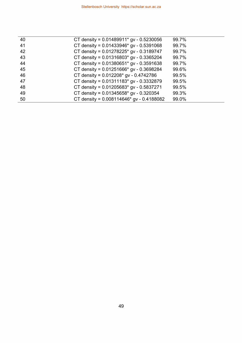
49

40 CT density = 0.01489911* gv - 0.5230056 99.7% 41 CT density = 0.01433946* gv - 0.5391068 99.7% 42 CT density = 0.01278225* gv - 0.3189747 99.7% 43 CT density = 0.01316803* gv - 0.3365204 99.7% 44 CT density = 0.01380651* gv - 0.3591638 99.7% 45 CT density = 0.01251666* gv - 0.3698284 99.6% 46 CT density = 0.012208* gv - 0.4742786 99.5% 47 CT density = 0.01311183* gv - 0.3332879 99.5% 48 CT density = 0.01205683* gv - 0.5837271 99.5% 49 CT density = 0.01345658* gv - 0.320354 99.3% 50 CT density = 0.008114646* gv - 0.4188082 99.0%


Greyscale - density calibration of an industrial CT scanner for ...

Documents