Green Skill Development Programme, MOEFCC, GoI– GSDP Manual FOREST ECOSYSTEM: GOODS AND SERVICES Forest Valuation: Understanding the Significance of Fragile Ecosystems RAMACHANDRA T V SUBASHCHANDRAN M D BHARATH S VINAY S G R RAO VISHNU MUKRI ENVIS, The Ministry of Environment, Forests and Cliamate Change, GoI ENVIS Technical Report : 142 Sahyadri Conservation Series: 79 May 2018 ENVironmental Information System[ENVIS] Sahyadri: Western Ghats Biodiversity Information System Centre for Ecological Sciences, Indian Institute of Science, Bangalore - 560012, INDIA Web: http://ces.iisc.ernet.in/biodiversity; http://ces.iisc.ernet.in/energy/, Email: [email protected]; [email protected] & ENVIS Centre: Karnataka State of Environment and Related Issues Environmental Management & Policy Research Institute Department of Forest, Ecology & Environment, Government of Karnataka, Bangalore 560 078 Web: http://karenvis.nic.in/Home.aspx, Email:[email protected], [email protected]

Welcome message from author
This document is posted to help you gain knowledge. Please leave a comment to let me know what you think about it! Share it to your friends and learn new things together.
Transcript
Green Skill Development Programme, MOEFCC, GoI– GSDP Manual
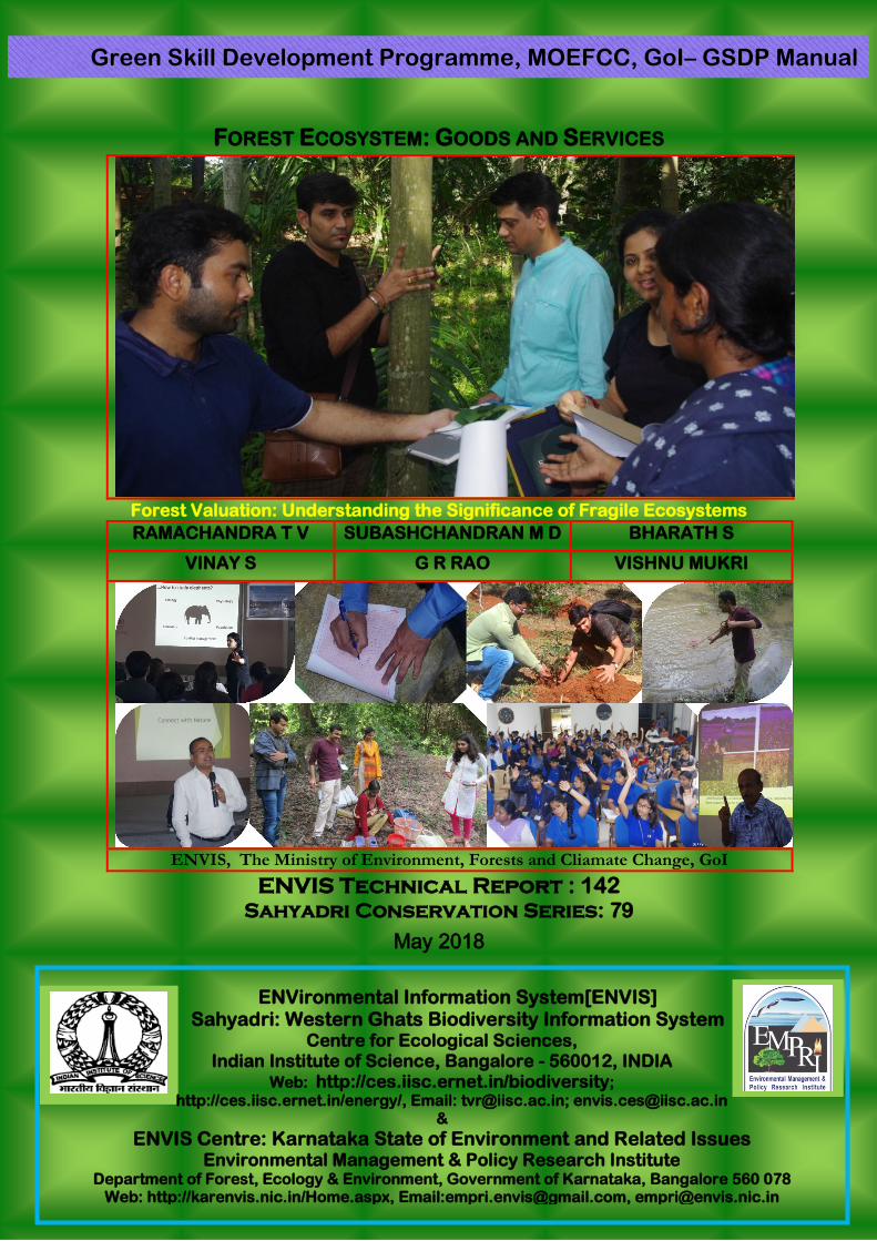
FOREST ECOSYSTEM: GOODS AND SERVICES
Forest Valuation: Understanding the Significance of Fragile Ecosystems
RAMACHANDRA T V SUBASHCHANDRAN M D BHARATH S
VINAY S G R RAO VISHNU MUKRI
ENVIS, The Ministry of Environment, Forests and Cliamate Change, GoI
ENVIS Technical Report : 142 Sahyadri Conservation Series: 79
May 2018
ENVironmental Information System[ENVIS] Sahyadri: Western Ghats Biodiversity Information System
Centre for Ecological Sciences, Indian Institute of Science, Bangalore - 560012, INDIA
Web: http://ces.iisc.ernet.in/biodiversity; http://ces.iisc.ernet.in/energy/, Email: [email protected]; [email protected]
&
ENVIS Centre: Karnataka State of Environment and Related Issues Environmental Management & Policy Research Institute
Department of Forest, Ecology & Environment, Government of Karnataka, Bangalore 560 078 Web: http://karenvis.nic.in/Home.aspx, Email:[email protected], [email protected]
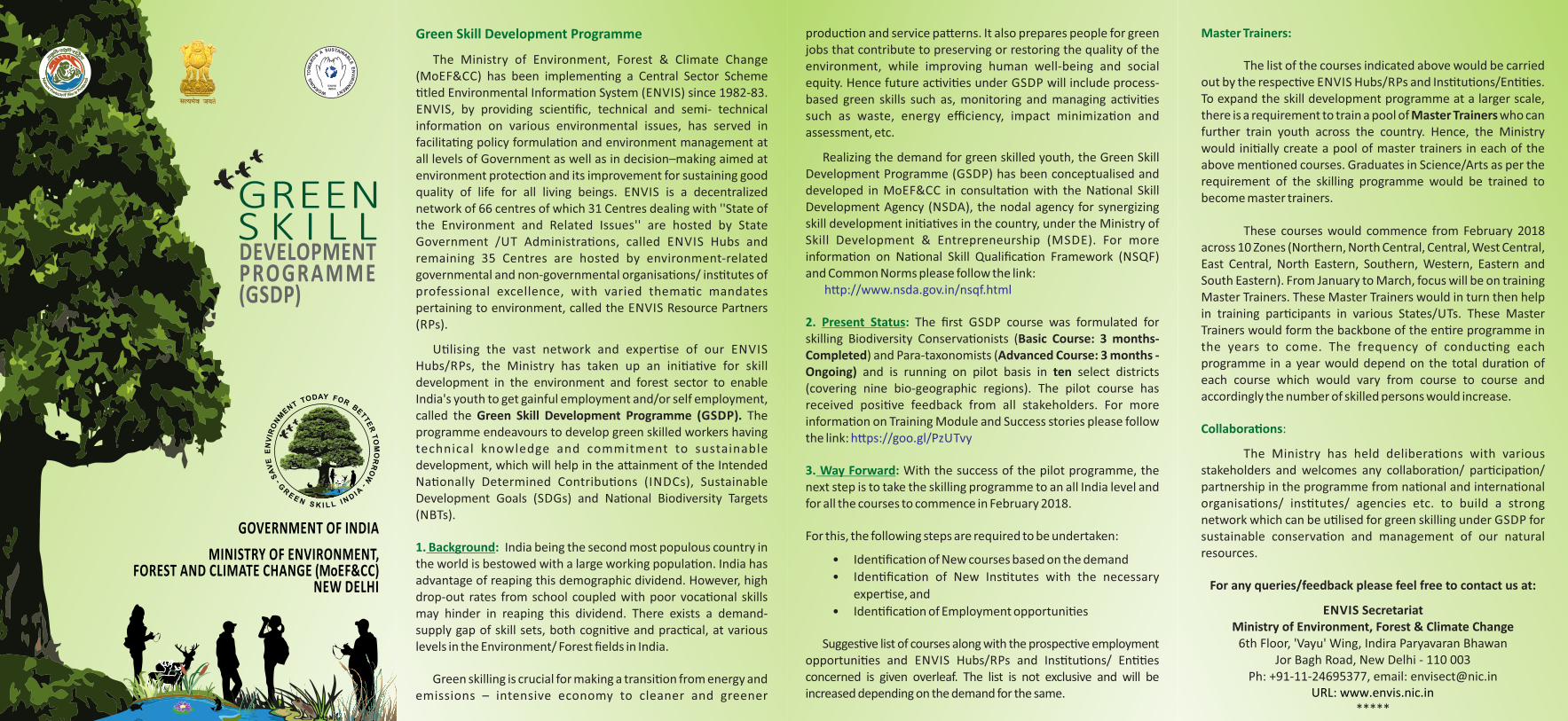
Green Skill Development Programme
The Ministry of Environment, Forest & Climate Change (MoEF&CC) has been implemen�ng a Central Sector Scheme �tled Environmental Informa�on System (ENVIS) since 1982-83. ENVIS, by providing scien�fic, technical and semi- technical informa�on on various environmental issues, has served in facilita�ng policy formula�on and environment management at all levels of Government as well as in decision–making aimed at environment protec�on and its improvement for sustaining good quality of life for all living beings. ENVIS is a decentralized network of 66 centres of which 31 Centres dealing with ''State of the Environment and Related Issues'' are hosted by State Government /UT Administra�ons, called ENVIS Hubs and remaining 35 Centres are hosted by environment-related governmental and non-governmental organisa�ons/ ins�tutes of professional excellence, with varied thema�c mandates pertaining to environment, called the ENVIS Resource Partners (RPs).
U�lising the vast network and exper�se of our ENVIS Hubs/RPs, the Ministry has taken up an ini�a�ve for skill development in the environment and forest sector to enable India's youth to get gainful employment and/or self employment, called the Green Skill Development Programme (GSDP). The programme endeavours to develop green skilled workers having technical knowledge and commitment to sustainable development, which will help in the a�ainment of the Intended Na�onally Determined Contribu�ons (INDCs), Sustainable Development Goals (SDGs) and Na�onal Biodiversity Targets (NBTs).
1. Background: India being the second most populous country in the world is bestowed with a large working popula�on. India has advantage of reaping this demographic dividend. However, high drop-out rates from school coupled with poor voca�onal skills may hinder in reaping this dividend. There exists a demand-supply gap of skill sets, both cogni�ve and prac�cal, at various levels in the Environment/ Forest fields in India.
Green skilling is crucial for making a transi�on from energy and emissions – intensive economy to cleaner and greener
produc�on and service pa�erns. It also prepares people for green jobs that contribute to preserving or restoring the quality of the environment, while improving human well-being and social equity. Hence future ac�vi�es under GSDP will include process-based green skills such as, monitoring and managing ac�vi�es such as waste, energy efficiency, impact minimiza�on and assessment, etc.
Realizing the demand for green skilled youth, the Green Skill Development Programme (GSDP) has been conceptualised and developed in MoEF&CC in consulta�on with the Na�onal Skill Development Agency (NSDA), the nodal agency for synergizing skill development ini�a�ves in the country, under the Ministry of Skill Development & Entrepreneurship (MSDE). For more informa�on on Na�onal Skill Qualifica�on Framework (NSQF) and Common Norms please follow the link:
h�p://www.nsda.gov.in/nsqf.html
2. Present Status: The first GSDP course was formulated for skilling Biodiversity Conserva�onists (Basic Course: 3 months-Completed) and Para-taxonomists (Advanced Course: 3 months -Ongoing) and is running on pilot basis in ten select districts (covering nine bio-geographic regions). The pilot course has received posi�ve feedback from all stakeholders. For more informa�on on Training Module and Success stories please follow the link: h�ps://goo.gl/PzUTvy
3. Way Forward: With the success of the pilot programme, the next step is to take the skilling programme to an all India level and for all the courses to commence in February 2018.
For this, the following steps are required to be undertaken:
• Iden�fica�on of New courses based on the demand
• Iden�fica�on of New Ins�tutes with the necessary
exper�se, and
• Iden�fica�on of Employment opportuni�es
Sugges�ve list of courses along with the prospec�ve employment opportuni�es and ENVIS Hubs/RPs and Ins�tu�ons/ En��es concerned is given overleaf. The list is not exclusive and will be increased depending on the demand for the same.
Master Trainers:
The list of the courses indicated above would be carried out by the respec�ve ENVIS Hubs/RPs and Ins�tu�ons/En��es. To expand the skill development programme at a larger scale, there is a requirement to train a pool of Master Trainers who can further train youth across the country. Hence, the Ministry would ini�ally create a pool of master trainers in each of the above men�oned courses. Graduates in Science/Arts as per the requirement of the skilling programme would be trained to become master trainers.
These courses would commence from February 2018 across 10 Zones (Northern, North Central, Central, West Central, East Central, North Eastern, Southern, Western, Eastern and South Eastern). From January to March, focus will be on training Master Trainers. These Master Trainers would in turn then help in training par�cipants in various States/UTs. These Master Trainers would form the backbone of the en�re programme in the years to come. The frequency of conduc�ng each programme in a year would depend on the total dura�on of each course which would vary from course to course and accordingly the number of skilled persons would increase.
Collabora�ons:
The Ministry has held delibera�ons with various stakeholders and welcomes any collabora�on/ par�cipa�on/ partnership in the programme from na�onal and interna�onal organisa�ons/ ins�tutes/ agencies etc. to build a strong network which can be u�lised for green skilling under GSDP for sustainable conserva�on and management of our natural resources.
For any queries/feedback please feel free to contact us at:
ENVIS SecretariatMinistry of Environment, Forest & Climate Change
6th Floor, 'Vayu' Wing, Indira Paryavaran BhawanJor Bagh Road, New Delhi - 110 003
Ph: +91-11-24695377, email: [email protected]
*****
GREENS K I L LDEVELOPMENTPROGRAMME(GSDP)
GOVERNMENT OF INDIA
MINISTRY OF ENVIRONMENT, FOREST AND CLIMATE CHANGE (MoEF&CC)
NEW DELHI
URL: www.envis.nic.in
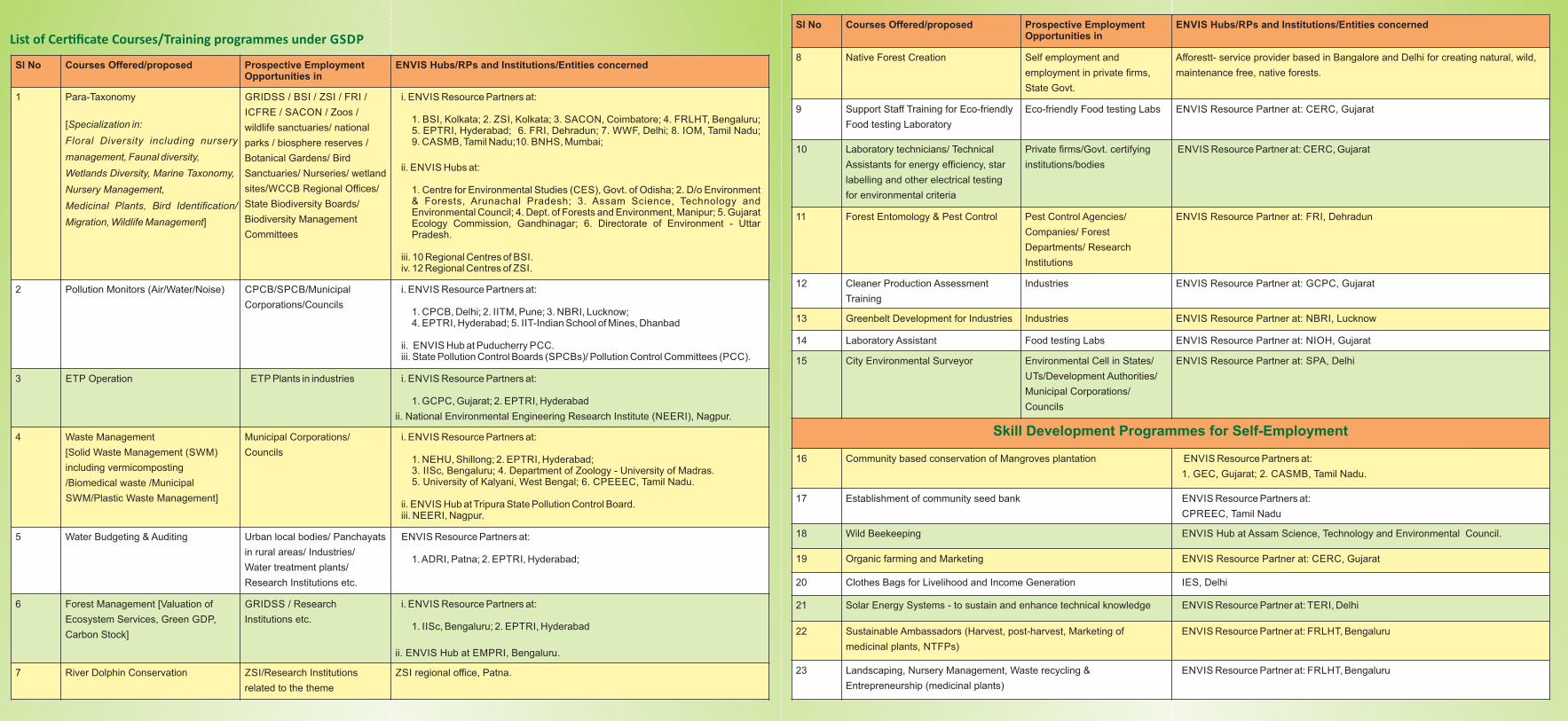
List of Cer�ficate Courses/Training programmes under GSDPSl No Courses Offered/proposed Prospective Employment
Opportunities inENVIS Hubs/RPs and Institutions/Entities concerned
8 Native Forest Creation Self employment and
employment in private firms,
State Govt.
Afforestt- service provider based in Bangalore and Delhi for creating natural, wild,
maintenance free, native forests.
9 Support Staff Training for Eco-friendly
Food testing Laboratory
Eco-friendly Food testing Labs ENVIS Resource Partner at: CERC, Gujarat
10 Laboratory technicians/ Technical
Assistants for energy efficiency, star
labelling and other electrical testing
for environmental criteria
Private firms/Govt. certifying
institutions/bodies
ENVIS Resource Partner at: CERC, Gujarat
11 Forest Entomology & Pest Control Pest Control Agencies/
Companies/ Forest
Departments/ Research
Institutions
ENVIS Resource Partner at: FRI, Dehradun
12 Cleaner Production Assessment
Training
Industries ENVIS Resource Partner at: GCPC, Gujarat
13 Greenbelt Development for Industries Industries ENVIS Resource Partner at: NBRI, Lucknow
14 Laboratory Assistant Food testing Labs ENVIS Resource Partner at: NIOH, Gujarat
15 City Environmental Surveyor Environmental Cell in States/
UTs/Development Authorities/
Municipal Corporations/
Councils
ENVIS Resource Partner at: SPA, Delhi
Skill Development Programmes for Self-Employment
16 Community based conservation of Mangroves plantation ENVIS Resource Partners at:
1. GEC, Gujarat; 2. CASMB, Tamil Nadu.
17 Establishment of community seed bank ENVIS Resource Partners at:
CPREEC, Tamil Nadu
18 Wild Beekeeping ENVIS Hub at Assam Science, Technology and Environmental Council.
19 Organic farming and Marketing ENVIS Resource Partner at: CERC, Gujarat
20 Clothes Bags for Livelihood and Income Generation IES, Delhi
21 Solar Energy Systems - to sustain and enhance technical knowledge ENVIS Resource Partner at: TERI, Delhi
22 Sustainable Ambassadors (Harvest, post-harvest, Marketing of
medicinal plants, NTFPs)
ENVIS Resource Partner at: FRLHT, Bengaluru
23 Landscaping, Nursery Management, Waste recycling &
Entrepreneurship (medicinal plants)
ENVIS Resource Partner at: FRLHT, Bengaluru
Sl No Courses Offered/proposed Prospective Employment Opportunities in
ENVIS Hubs/RPs and Institutions/Entities concerned
1 Para-Taxonomy
[Specialization in:
Floral Diversity including nursery
management, Faunal diversity,
Wetlands Diversity, Marine Taxonomy,
Nursery Management,
Medicinal Plants, Bird Identification/
Migration, Wildlife Management]
GRIDSS / BSI / ZSI / FRI /
ICFRE / SACON / Zoos /
wildlife sanctuaries/ national
parks / biosphere reserves /
Botanical Gardens/ Bird
Sanctuaries/ Nurseries/ wetland
sites/WCCB Regional Offices/
State Biodiversity Boards/
Biodiversity Management
Committees
i. ENVIS Resource Partners at:
1. BSI, Kolkata; 2. ZSI, Kolkata; 3. SACON, Coimbatore; 4. FRLHT, Bengaluru; 5. EPTRI, Hyderabad; 6. FRI, Dehradun; 7. WWF, Delhi; 8. IOM, Tamil Nadu; 9. CASMB, Tamil Nadu;10. BNHS, Mumbai;
ii. ENVIS Hubs at:
1. Centre for Environmental Studies (CES), Govt. of Odisha; 2. D/o Environment & Forests, Arunachal Pradesh; 3. Assam Science, Technology and Environmental Council; 4. Dept. of Forests and Environment, Manipur; 5. Gujarat Ecology Commission, Gandhinagar; 6. Directorate of Environment - Uttar Pradesh.
iii. 10 Regional Centres of BSI. iv. 12 Regional Centres of ZSI.
2 Pollution Monitors (Air/Water/Noise) CPCB/SPCB/Municipal
Corporations/Councils
i. ENVIS Resource Partners at:
1. CPCB, Delhi; 2. IITM, Pune; 3. NBRI, Lucknow; 4. EPTRI, Hyderabad; 5. IIT-Indian School of Mines, Dhanbad
ii. ENVIS Hub at Puducherry PCC.iii. State Pollution Control Boards (SPCBs)/ Pollution Control Committees (PCC).
3 ETP Operation ETP Plants in industries i. ENVIS Resource Partners at:
1. GCPC, Gujarat; 2. EPTRI, Hyderabad
ii. National Environmental Engineering Research Institute (NEERI), Nagpur.
4 Waste Management
[Solid Waste Management (SWM)
including vermicomposting
/Biomedical waste /Municipal
SWM/Plastic Waste Management]
Municipal Corporations/
Councils
i. ENVIS Resource Partners at:
1. NEHU, Shillong; 2. EPTRI, Hyderabad;3. IISc, Bengaluru; 4. Department of Zoology - University of Madras. 5. University of Kalyani, West Bengal; 6. CPEEEC, Tamil Nadu.
ii. ENVIS Hub at Tripura State Pollution Control Board.iii. NEERI, Nagpur.
5 Water Budgeting & Auditing Urban local bodies/ Panchayats
in rural areas/ Industries/
Water treatment plants/
Research Institutions etc.
ENVIS Resource Partners at:
1. ADRI, Patna; 2. EPTRI, Hyderabad;
6 Forest Management [Valuation of
Ecosystem Services, Green GDP,
Carbon Stock]
GRIDSS / Research
Institutions etc.
i. ENVIS Resource Partners at:
1. IISc, Bengaluru; 2. EPTRI, Hyderabad
ii. ENVIS Hub at EMPRI, Bengaluru.
7 River Dolphin Conservation ZSI/Research Institutions
related to the theme
ZSI regional office, Patna.
GSDP: Course on “Valuation of ecosystem goods and services” ENVIS TECHNICAL REPORT 142, LECTURE NOTES
1 The views expressed in the publication [ETR 142] are of the authors and not necessarily reflect the views of either the publisher,
funding agencies or of the employer (Copyright Act, 1957; Copyright Rules, 1958, The Government of India).
© ENVIS, IISc, Green Skill Development Programme
FOREST ECOSYSTEM - GOODS AND SERVICES Citation: Ramachandra T V, Subashchandran M D, Bharath Setturu, Vinay S, Bharath H Aithal, G R Rao,
2018. Forest Ecosystem: Goods and Services, ENVIS Technical Report 142, Sahyadri Conservation Series
79, ENVIS, CES, Indian Institute of Science, Bangalore 560012, Pp 312
RAMACHANDRA T V SUBASHCHANDRAN M D BHARATH S
VINAY S BHARATH H. AITHAL G R RAO
ENVIS, The Ministry of Environment, Forests and Cliamate Change, GoI
Sponsored by
ENVIS Division, The Ministry of Environment, Forests and Climate Change, GoI
SAHYADRI CONSERVATION SERIES:79
Sahyadri- Environmental Information System, [ENVIS]
Centre for Ecological Sciences, CES TE 15 Indian Institute of Science
Email: [email protected]; [email protected] Web: http://wgbis.ces.iisc.ernet.in/biodiversity
Tel: 080-2293 3099/ 2293 3503
GSDP: Course on “Valuation of ecosystem goods and services” ENVIS TECHNICAL REPORT 142, LECTURE NOTES
2 The views expressed in the publication [ETR 142] are of the authors and not necessarily reflect the views of either the publisher,
funding agencies or of the employer (Copyright Act, 1957; Copyright Rules, 1958, The Government of India).
© ENVIS, IISc, Green Skill Development Programme
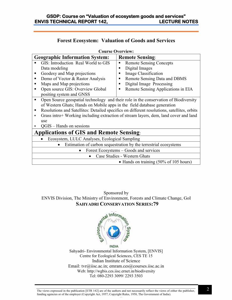
Forest Ecosystem: Valuation of Goods and Services
Course Overview:
Geographic Information System: Remote Sensing:
GIS: Introduction Real World to GIS
Data modeling
Geodesy and Map projections
Demo of Vector & Rastor Analysis
Maps and Map projections
Open source GIS: Overview Global
positing system and GNSS
Remote Sensing Concepts
Digital Images
Image Classification
Remote Sensing Data and DBMS
Digital Image Processing
Remote Sensing Applications in EIA
Open Source geospatial technology and their role in the conservation of Biodiversity
of Western Ghats; Hands on Mobile apps in the field database generation
Resolutions and Satellites: Detailed specifics on different resolutions, satellites, orbits
Grass intro+ Working including extraction of stream layers, dem, land cover and land
use
QGIS – Hands on sessions
Applications of GIS and Remote Sensing:
Ecosystem, LULC Analyses, Ecological Sampling
Estimation of carbon sequestration by the terrestrial ecosystems
Forest Ecosystems – Goods and services
Case Studies - Western Ghats
Hands on training (50% of 105 hours)
Sponsored by
ENVIS Division, The Ministry of Environment, Forests and Climate Change, GoI
SAHYADRI CONSERVATION SERIES:79
Sahyadri- Environmental Information System, [ENVIS]
Centre for Ecological Sciences, CES TE 15 Indian Institute of Science
Email: [email protected]; [email protected] Web: http://wgbis.ces.iisc.ernet.in/biodiversity
Tel: 080-2293 3099/ 2293 3503
GSDP: Course on “Valuation of ecosystem goods and services” ENVIS TECHNICAL REPORT 142, LECTURE NOTES
3 The views expressed in the publication [ETR 142] are of the authors and not necessarily reflect the views of either the publisher,
funding agencies or of the employer (Copyright Act, 1957; Copyright Rules, 1958, The Government of India).
© ENVIS, IISc, Green Skill Development Programme
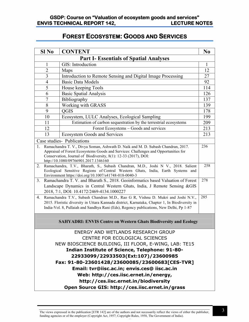
FOREST ECOSYSTEM: GOODS AND SERVICES
Sl No CONTENT No
Part I- Essentials of Spatial Analyses 1 GIS: Introduction 1
2 Maps 12
3 Introduction to Remote Sensing and Digital Image Processing 27
4 Basic Data Models 92
5 House keeping Tools 114
6 Basic Spatial Analysis 126
7 Bibliography 137
8 Working with GRASS 139
9 QGIS 178
10 Ecosystem, LULC Analyses, Ecological Sampling 199
11 Estimation of carbon sequestration by the terrestrial ecosystems 209
12 Forest Ecosystems – Goods and services 213
13 Ecosystem Goods and Services 213
Case studies- Publications 1. Ramachandra T. V., Divya Soman, Ashwath D. Naik and M. D. Subash Chandran, 2017.
Appraisal of Forest Ecosystems Goods and Services: Challenges and Opportunities for
Conservation, Journal of Biodiversity, 8(1): 12-33 (2017), DOI:
http://10.1080/09766901.2017.1346160
236
2. Ramachandra, T.V., Bharath, S., Subash Chandran, M.D., Joshi N V., 2018. Salient
Ecological Sensitive Regions of Central Western Ghats, India, Earth Systems and
Environment https://doi.org/10.1007/s41748-018-0040-3
258
3. Ramachandra T. V. and Bharath S., 2018. Geoinformatics based Valuation of Forest
Landscape Dynamics in Central Western Ghats, India, J Remote Sensing &GIS
2018, 7:1, DOI: 10.4172/2469-4134.1000227
278
4. Ramachandra T.V., Subash Chandran M.D., Rao G R, Vishnu D. Mukri and Joshi N.V.,
2015. Floristic diversity in Uttara Kannada district, Karnataka, Chapter 1, In Biodiversity in
India-Vol. 8, Pullaiah and Sandhya Rani (Eds), Regency publications, New Delhi, Pp 1-87
285
SAHYADRI: ENVIS Centre on Western Ghats Biodiversity and Ecology
ENERGY AND WETLANDS RESEARCH GROUP
CENTRE FOR ECOLOGICAL SCIENCES
NEW BIOSCIENCE BUILDING, III FLOOR, E-WING, LAB: TE15
Indian Institute of Science, Telephone: 91-80-
22933099/22933503(Ext:107)/23600985
Fax: 91-80-23601428/23600085/23600683[CES-TVR]
Email: [email protected]; envis.ces@ iisc.ac.in
Web: http://ces.iisc.ernet.in/energy,
http://ces.iisc.ernet.in/biodiversity
Open Source GIS: http://ces.iisc.ernet.in/grass
GSDP: Course on “Valuation of ecosystem goods and services” 2018
1 © ENVIS, IISc, Green Skill Development Programme
GIS: Introduction
Many of our decisions depend on the details of our immediate surrounding, and require
information about specific places on the Earth’s surface. In this regard, recent
developments in information technologies have opened a vast potential in
communication, analysis of spatial and temporal data. Data representing the real world
can be stored and processed so that they can be presented later in a simplified form to
suite specific needs. Such information is called geographical because it helps us to
distinguish one place from another and to make decisions for one place that are
appropriate for that location. Geographical information allows us to apply general
principles to the specific conditions of each location, allows us to track what is happening
at any place, and helps us to understand how one place differs from another. Spatial
information is essential for effective planning and decision-making at regional, national
and global levels. The geographical information in the form of maps (based on field
surveys), photos taken from aircraft (aerial photography), and images collected from the
space borne platforms (satellite) can be represented in digital form, this opens an
enormous range of possibilities for communication, analysis, modeling, and accurate
decision making, but a degree of approximation.
GIS can be defined as computerized information storage processing and retrieval system
that has hardware, software specially designed to cope with geographically referenced
spatial data. Collective name for such system is geographical information systems,
(GISs). Processing geographical information include:
Techniques to input geographical information, converting the information to
digital form
Technique for sorting such information in a compact format on computer disks,
and other digital storage media
Methods for automated analysis for geographical data, to search for the patterns,
combine different kinds of data, make measurements find optimum sites or routes,
and a host of other tasks
(c) E
NVIS, I
ISc,
2018
GSDP: Course on “Valuation of ecosystem goods and services” 2018
2 © ENVIS, IISc, Green Skill Development Programme
Methods to predict the out come of various scenarios, such as the effects of
climate change on vegetation
Techniques for display of data in the form of maps, images and other kinds of
display
Capabilities for output of results in the form of numbers and tables.
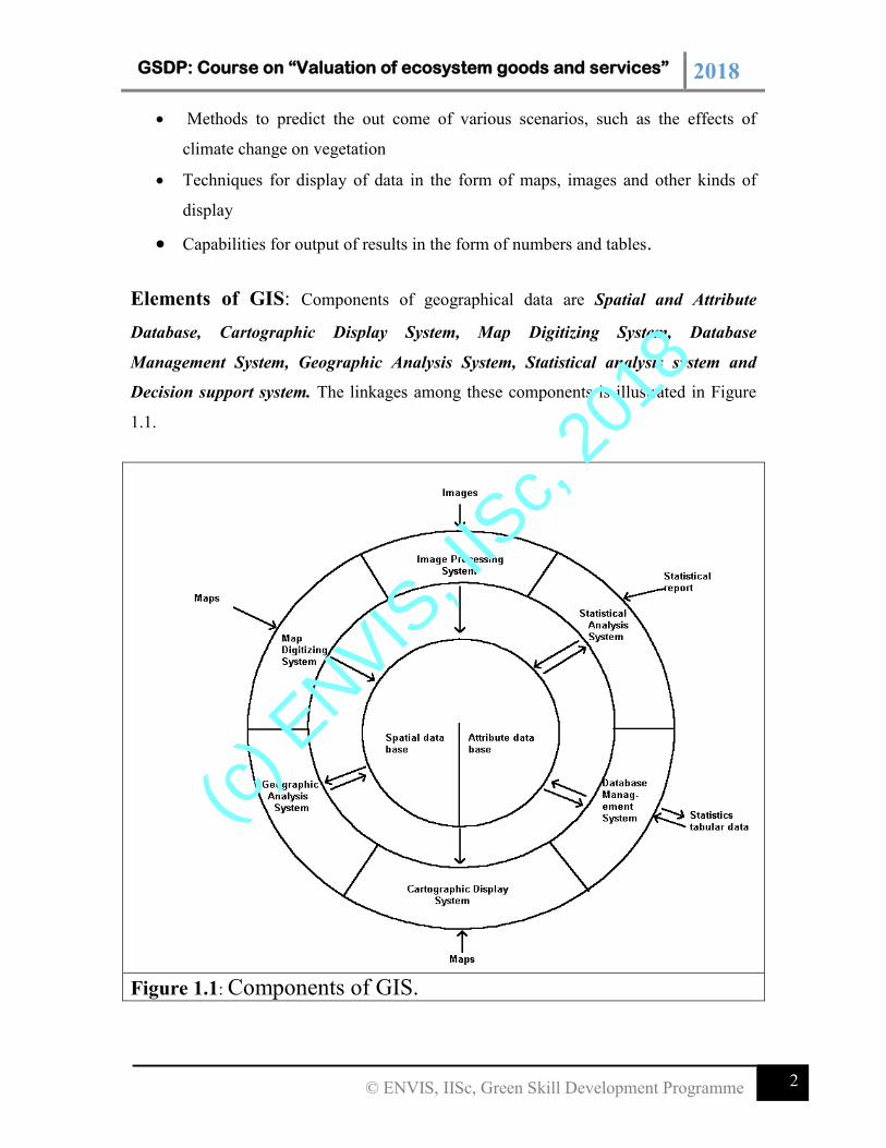
Elements of GIS: Components of geographical data are Spatial and Attribute
Database, Cartographic Display System, Map Digitizing System, Database
Management System, Geographic Analysis System, Statistical analysis system and
Decision support system. The linkages among these components is illustrated in Figure
1.1.
Figure 1.1: Components of GIS.
(c) E
NVIS, I
ISc,
2018
GSDP: Course on “Valuation of ecosystem goods and services” 2018
3 © ENVIS, IISc, Green Skill Development Programme
i). Spatial and Attribute Database: Central to the system is the database – a collection
of maps and associated information in digital form. Since the database is concerned
with earth surface features, it is seen to comprise of two elements – a spatial database
describing the geology (shape and position) of the earth surface features, and an
attribute database describing the characteristics or quantities of these features. Thus,
for example, we might have a property parcel defined in the spatial database and
qualities such as its land use, owner, property valuation, etc. in the attribute database.
ii). Cartographic Display System: Surrounding the central database, we have a series of
software components. The most basic of these is the cartographic display system. The
cartographic display system allows one to take selected elements of the database and
produce map output on the screen or some hardcopy device such as printer or plotter.
iii). Map Digitizing System: After cartographic display, the next most essential element is
a Map Digitization System. With a map digitizing system, one can take existing paper
maps and convert them into digital form, thus further developing the database. In the
most common method of digitizing, one attaches the paper map to a digitizing tablet
or board and then traces the features of interest with a stylus according to the
procedures required for digitizing. Many maps digitizing system also allows for some
editing of the digitized data. Scanners can also be used to digitize data such as aerial
photographs. The results is a graphic image, rather than the outlines of features that
are created with a variety of standard graphics file formats for export. These files are
then imported into the GIS. Computer assisted design (CAD) and Coordinate
Geometry (COGO) are two examples of software systems that provide the ability to
add digitized map information to the database, in addition to providing cartographic
display capabilities.
iv). Database Management System: The next logical component in a GIS is Database
Management System (DBMS), which is used to input, manage and analyze attribute
information along with then spatial data. GIS thus typically incorporates a variety of
utilities to manage the spatial and attribute components of the geographic data.
DBMS aids to enter attribute data, such as tabular information and statistics, and
(c) E
NVIS, I
ISc,
2018
GSDP: Course on “Valuation of ecosystem goods and services” 2018
4 © ENVIS, IISc, Green Skill Development Programme
subsequently extract specialized tabulations and statistical summaries to provide new
tabular reports. The DBMS provides the ability to analyze attribute data. Many map
analysis have no true spatial component, and for these a DBMS will often function
quite well. For example, we might inquire of the system to find all property parcels
where the head of the household is single but with one or more child dependents, and
to produce a spatial map. Software that provides cartographic display, map digitizing,
and database query capabilities are often referred to as Automated Mapping and
Facilities Management (AM/FM) system.
v). Geographic Analysis System: Up to this point, we have described a very powerful set
of capabilities that the GIS offer, the ability to digitize spatial data and attach attribute
to the features stored; to analyze these data based on those attribute; and to map to the
result. But on inclusion geographic analysis system, we extend the capabilities of the
traditional database query to include the ability to analyze data based on their
location. Perhaps the simplest example of this is to consider what happens when we
are concerned with the joint occurrence of features with different geographies. For
example, suppose we want to find all areas of residential land on bedrock types
associated with high levels of radon gas. A traditional DBMS cannot solve this
problem because bedrock types and landuse divisions simply do not share the same
geography. Traditional database query is fine as long as we are taking about attributes
belonging to the same features. But when the features are different, it cannot cope.
For this we need a GIS. In fact, it is this ability to compare different feature based on
their common geographic occurrence that is the hallmark of GIS. This analysis is
accomplished by the process of overlay, thus named because it is identical in
character to overlaying transparent maps of the two entity groups on top of one
another. Like the DBMS, the Geographic Analysis System as highlighted in Figure
1.1 has a two-way interaction with the database; the process is distinctly analytical in
character. Thus while it may access data from the database, it may equally contribute
the results of that analysis as a new addition to the database. For example we might
look for joint occurrence of lands on steep slopes with erodable soil under agriculture
and call the results based on existing data and set of specific relations. Thus the
(c) E
NVIS, I
ISc,
2018
GSDP: Course on “Valuation of ecosystem goods and services” 2018
5 © ENVIS, IISc, Green Skill Development Programme
analytic capabilities of the Geographic Analysis System and the DBMS play a vital
role in extending the database through the addition of knowledge of relationships
between features.
vi). Image Processing System: In addition to these essential GIS elements, remotely
sensed image and specialized statistical analysis are also important. This we will
discuss in the subsequent sections.
vii). Statistical analysis system: GIS incorporates a series of specialized routines for
analyzing the statistical description of spatial data and for inferences drawn from
statistical procedures.
viii). Decision support system (DSS): Decision support constitutes a vital function of a
GIS. It helps in the construction of multi-criteria suitability maps, and address
allocation decisions when there is multiple objectives involved while accounting for
error in the process. Used in conjunction with the other components of the system,
DSS provides a powerful tool in decision-making for resource allocation.
Map Data Representation
A Geographic Information System stores two types of data that are found on a map—the
geographic definitions of earth surface features and the attributes or qualities that those
features possess. Most systems use nearly one or a combination of both the fundamental
map representation techniques: vector and raster.
Vector: This refers to the spatial data represented in the form of point, line or polygon
depending on the feature of interest (and scale). With vector representation, the
boundaries or the course of the features are defined by a series of points that, when joined
with straight lines, form the graphic representation of that feature. The points themselves
are encoded with a pair of numbers giving the X and Y coordinates in systems such as
latitude/ longitude, etc. The attributes of features are then stored in the database
management system (DBMS). For example, a vector map of property parcels might be
tied to an attribute database of information containing the address, owner’s name,
(c) E
NVIS, I
ISc,
2018
GSDP: Course on “Valuation of ecosystem goods and services” 2018
6 © ENVIS, IISc, Green Skill Development Programme
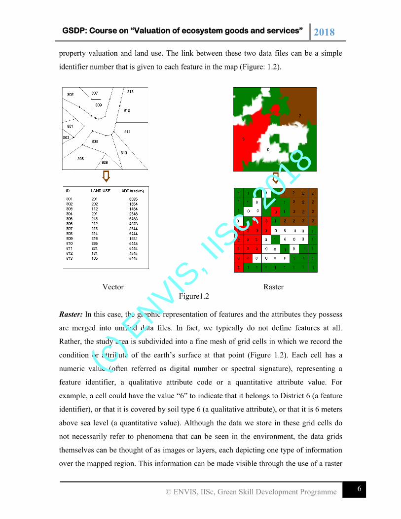
property valuation and land use. The link between these two data files can be a simple
identifier number that is given to each feature in the map (Figure: 1.2).
Raster: In this case, the graphic representation of features and the attributes they possess
are merged into unified data files. In fact, we typically do not define features at all.
Rather, the study area is subdivided into a fine mesh of grid cells in which we record the
condition or attribute of the earth’s surface at that point (Figure 1.2). Each cell has a
numeric value (often referred as digital number or spectral signature), representing a
feature identifier, a qualitative attribute code or a quantitative attribute value. For
example, a cell could have the value “6” to indicate that it belongs to District 6 (a feature
identifier), or that it is covered by soil type 6 (a qualitative attribute), or that it is 6 meters
above sea level (a quantitative value). Although the data we store in these grid cells do
not necessarily refer to phenomena that can be seen in the environment, the data grids
themselves can be thought of as images or layers, each depicting one type of information
over the mapped region. This information can be made visible through the use of a raster
Vector Raster
Figure1.2
(c) E
NVIS, I
ISc,
2018
GSDP: Course on “Valuation of ecosystem goods and services” 2018
7 © ENVIS, IISc, Green Skill Development Programme
display. In a raster display, such as the screen on your computer, there is also a grid of
small cells called pixels (or picture elements). The word pixel is a contraction of the term
picture element. Pixels vary in their color, shape or gray tone depending on features in
the object. To make an image, the cell values in the data grid are used to regulate directly
the graphic appearance of their corresponding pixels. Thus in a raster system, the data
directly controls the visible form we see.
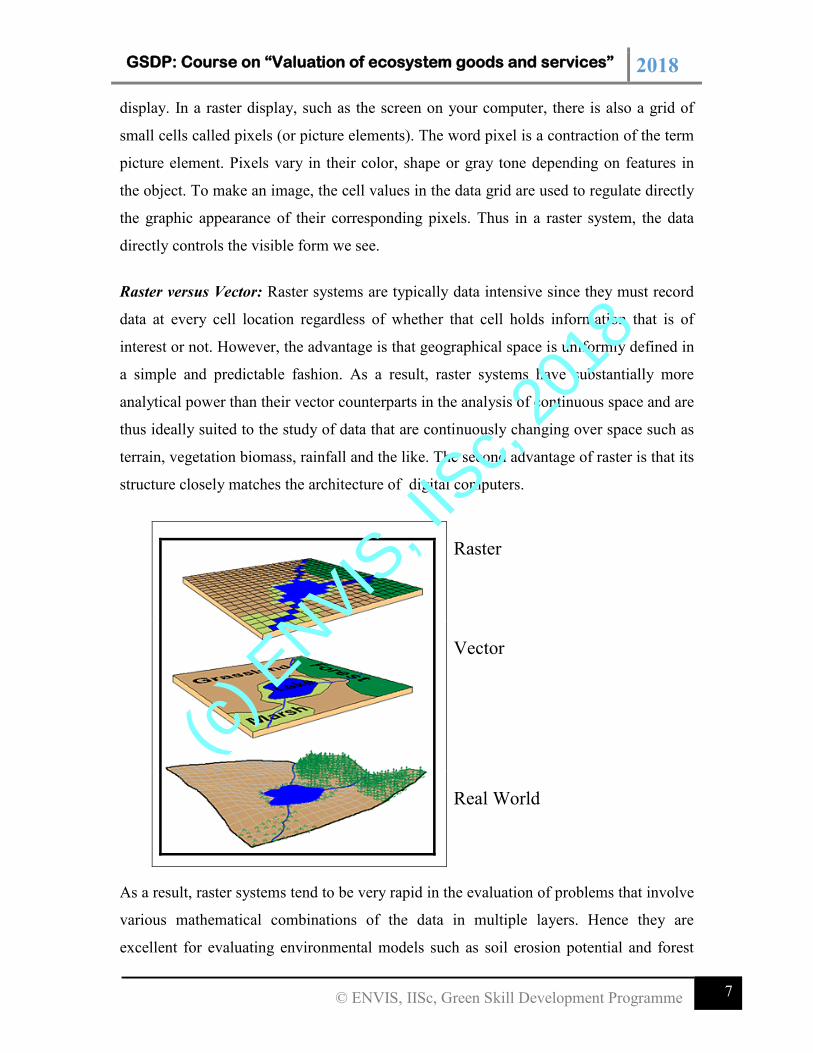
Raster versus Vector: Raster systems are typically data intensive since they must record
data at every cell location regardless of whether that cell holds information that is of
interest or not. However, the advantage is that geographical space is uniformly defined in
a simple and predictable fashion. As a result, raster systems have substantially more
analytical power than their vector counterparts in the analysis of continuous space and are
thus ideally suited to the study of data that are continuously changing over space such as
terrain, vegetation biomass, rainfall and the like. The second advantage of raster is that its
structure closely matches the architecture of digital computers.
Raster
Vector
Real World
As a result, raster systems tend to be very rapid in the evaluation of problems that involve
various mathematical combinations of the data in multiple layers. Hence they are
excellent for evaluating environmental models such as soil erosion potential and forest
(c) E
NVIS, I
ISc,
2018
GSDP: Course on “Valuation of ecosystem goods and services” 2018
8 © ENVIS, IISc, Green Skill Development Programme
management suitability. In addition, since satellite imagery employs a raster structure,
most raster systems can easily incorporate these data, and some provide full image
processing capabilities.
While raster systems are predominantly analysis oriented, vector systems tend to be more
database management oriented. Vector systems are quite efficient in their storage of map
data because they only store the boundaries of features and not that which is inside those
boundaries. Because the graphic representation of features is directly linked to the
attribute database, vector systems usually allow one to roam around the graphic display
with a mouse and query the attributes associated with a displayed feature, such as the
distance between points or along lines, the areas of regions defined on the screen, and so
on. In addition, they can produce simple thematic maps of database queries.
Compared to their raster counterparts, vector systems do not have as extensive a range of
capabilities for analyses over continuous space. They do, however, excel at problems
concerning movements over a network and can undertake the most fundamental of GIS
operations that will be sketched out below. For many, it is simple database management
functions and excellent mapping capabilities that make vector systems attractive. Because
of the close affinity between the logic of vector representation and traditional map
production, a pen plotter can be driven to produce a map that is in distinguishable from
that produce by traditional means. As a result, vector systems are very popular in
municipal applications where issues of engineering map production and database
management predominate.
Geographic database concepts: Regardless of the logic used for spatial representation,
raster and vector, we begin to see that a geographic database as a complete database for a
given region and is organized in a fashion similar to a collection of maps. Vector systems
come closest to this logic with what are known as coverages. Map like collection that
contain the geographic definition of a set of features and their associated attributes tables.
However, they differ from maps in two ways. First, each will typically contain
information on only a single feature types, such property parcels, soil polygons, and the
like. Second, they may contain a whole series of attributes that pertain to those features,
(c) E
NVIS, I
ISc,
2018
GSDP: Course on “Valuation of ecosystem goods and services” 2018
9 © ENVIS, IISc, Green Skill Development Programme
such as a set of census information for city blocks.
Raster system also uses this map like logic, but usually divide data sets into unitary
layers. A layer contains all the data for a single attribute. Thus one might have a soil
layer, a road layer and a land-use layer.
There are subtle differences, for all intents and purposes, raster layer and vector coverage
can be thought of as simply different manifestations of the same concepts as the
organization of the database into elementary map-like themes. Layers and coverage differ
from traditional paper maps, however, in an important way. When a map is digitized,
scale differences are removed. The digital data may be displayed or printed at any scale.
More importantly, digital data layers that were derived from maps of different scale, but
covering the same geographic area, may be combined.
GIS provide utilities for changing the projection and reference system of digital layers.
This allows multiple layers, digitized from maps having various projections and reference
system, to be converted to a common system.
With the ability to manage differences of scale, projection and reference system, layers
can be merged with ease, elimination a problem that has traditionally hampered planning
activities with maps. It is important to note, however, that the issue of resolution of the
information in the data layers remains. Although features digitized from a poster sized
world map could be combined in a GIS with features digitized from very large-scale local
map, such as a city street map, this would normally not be done. The level of accuracy
and detail of the digital data can be as good as that of the original maps.
Georeferencing: All spatial data files in GIS are georeferenced. Georeferencing refers
to the location of a layer or coverage in the space as a definition by a known coordinate
referring system. With raster images, a common form of georeferencing is to indicate the
reference system, the reference units and the coordinate positions of the left, right, top,
and bottom edges of the image. The same is true of the vector data files, although the left,
right, top and bottom edges now refer to what is commonly called the bounding rectangle
(c) E
NVIS, I
ISc,
2018
GSDP: Course on “Valuation of ecosystem goods and services” 2018
10 © ENVIS, IISc, Green Skill Development Programme
of the coverage; rectangle which defines the limit of the mapped area (corners of a
feature). This information is particularly important in an integrated GIS since it allows
raster and vector files to be related to one another in a reliable and meaningful way. It is
also vital for the referencing of the data values to actual positions on the ground.
GIS Applicability: The society is so complex, and their activities so interwoven, that
no problem can be considered in isolation or with out regard for the full range of its
interconnections. For example, a new housing development will affect the local school
system. The volume of city traffic put constraints on the maintenance of buried pipe
networks, affecting health. The action needed to solve such a problems are best taken on
the basis of standardized information that can be combined in many ways to serve many
users. GISs have this capability.
Environmental and resource management: Decision making is becoming increasing
complex as dwindling natural resources and more demanding economic priorities
diminish the chances of today’s decision being right tomorrow. Furthermore,
environmental awareness is constantly increasing among the general public, particularly
among the younger generation. To help us map and monitor changes, and plan
appropriate responses that take account of the complex interactions of the Earth system,
many countries now have comprehensive programs to capture and archive information on
the existing natural resources and known sources of pollution, using technologies such as
satellite remote sensing and GIS. The data may be used both to expose conflicts and to
examine environmental impacts and even simulate the causes and the alternative will
become possible.
Planning and development: The planning and development of new housing, roads,
and industrial facilities require data on the terrain and other geographical information.
Development often involves building on marginal terrain, increasing the density of the
building in the areas already built up, or both. Yet the new structures must fit with in the
existing technical infrastructure; here computerization is a great aid. One of the benefits
GIS holds for such projects is a minimalization of disruption to the existing
infrastructure.
(c) E
NVIS, I
ISc,
2018
GSDP: Course on “Valuation of ecosystem goods and services” 2018
11 © ENVIS, IISc, Green Skill Development Programme
Escalating construction costs have made the optimizing of building and road location
extremely important. Minimizing blasting and earthmoving are significant aspect of
minimizing costs. Flexibility is vital: plans should be amenable to rapid changes as
decisions are made. The influence of special interest groups and individual citizens
require that initial plans be presented effectively and in a manner that is easily
understood. Simplified, visualized plans are instrumental in conveying both the content
of the scheme and the nature of any likely impact on those concerned.
Management and public services: In modern societies, decisions should be made
quickly, using reliable data, even though there may be many differing viewpoints to
consider and large amount of information to process. Today, the impact of development
decisions is ever greater, involving conflicts between society and individuals, or between
development and preservation. Information must therefore be readily available to
decision makers; the majority of such information is likely to be geographical in nature,
and best handled using GIS.
Overviews of administrative units and properties are crucial in the development of both
virgin terrain and built-up area, in both developed and developing nations. In many
countries, property registration is extensive: even in smaller states, 2 to 3 million
properties maybe involved. Moreover, property is also an economic factor in taxation and
security for loans; so comprehensive overviews are essential to a well-ordered society.
Computerized registers based on GIS technology are now well established in many
countries.
Land transportation: In many countries, the greater part of transportation has
shifted from rail to road, at the same time, the use of private vehicle has greatly
increased. These developments have created traffic problems, which cause loss of time
and money. Large goods are now transported by road. In most countries the annual costs
of traffic accidents have become extremely high. The automobile industry is now
investing heavily in the development of driver information system, and several systems
are now in the market. In principle, all of them involve simple GIS function with digital
maps and supplementary information.
(c) E
NVIS, I
ISc,
2018
GSDP: Course on “Valuation of ecosystem goods and services” 2018
16 © ENVIS, IISc, Green Skill Development Programme
Chapter 2: Maps
Map is a picture of a place as our eyes see it or best-known models of real world. Maps
have been used for thousands of years to represent information about the real world.
Their conception and design has developed into a science with a high degree of
sophistication. Maps have proven to be extremely useful for many applications in various
domains.
A disadvantage of maps is that they are restricted to two-dimensional static
representation, and that they always are displayed in a given scale. The map scale
determines the spatial resolution of the graphic feature representation. The smaller the
scales, the less detail a map can show. The accuracy of the base data, on the other hand,
puts limits to the scale in which a map can sensibly drawn. The selection of proper map is
one of the first and most important steps in map design.
A map is always a graphic representation at certain level of detail, which is determined
by the scale. Map sheets have physical boundaries, and features spanning two map sheets
have to cut into pieces.
Cartography as the science and art of map making functions as an interpreter translating
real world phenomena into correct, clear and understandable representation for our use.
Maps also become a data source for other maps.
Maps are made for many reasons and, therefore they vary in content and context.
Different maps show different information. Different symbols are used to represent the
features of the environment on a map. They are explained in the legend for each map.
Some examples
A photograph: A photograph shows a place as our eyes see it. However, the area that
is viewed on the ground is limited. It is often difficult to see a substantial landscape in a
single photography.
(c) E
NVIS, I
ISc,
2018
GSDP: Course on “Valuation of ecosystem goods and services” 2018
17 © ENVIS, IISc, Green Skill Development Programme
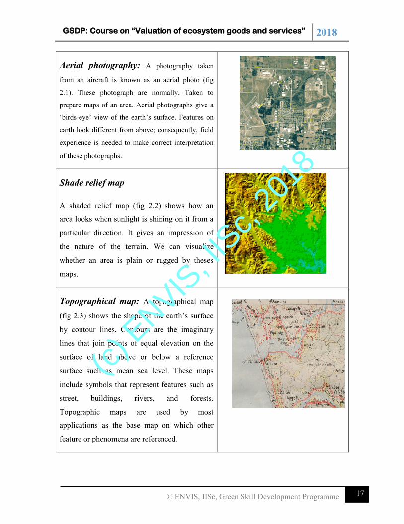
Aerial photography: A photography taken
from an aircraft is known as an aerial photo (fig
2.1). These photograph are normally. Taken to
prepare maps of an area. Aerial photographs give a
‘birds-eye’ view of the earth’s surface. Features on
earth look different from above; consequently, field
experience is needed to make correct interpretation
of these photographs.
Shade relief map
A shaded relief map (fig 2.2) shows how an
area looks when sunlight is shining on it from a
particular direction. It gives an impression of
the nature of the terrain. We can visualize
whether an area is plain or rugged by theses
maps.
Topographical map: A topographical map
(fig 2.3) shows the shape of the earth’s surface
by contour lines. Contours are the imaginary
lines that join points of equal elevation on the
surface of land above or below a reference
surface such as mean sea level. These maps
include symbols that represent features such as
street, buildings, rivers, and forests.
Topographic maps are used by most
applications as the base map on which other
feature or phenomena are referenced.
(c) E
NVIS, I
ISc,
2018
GSDP: Course on “Valuation of ecosystem goods and services” 2018
18 © ENVIS, IISc, Green Skill Development Programme
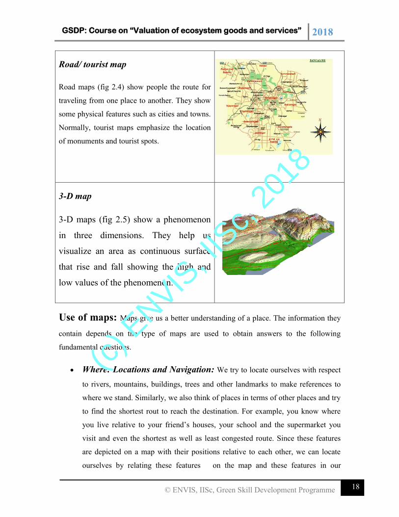
Road/ tourist map
Road maps (fig 2.4) show people the route for
traveling from one place to another. They show
some physical features such as cities and towns.
Normally, tourist maps emphasize the location
of monuments and tourist spots.
3-D map
3-D maps (fig 2.5) show a phenomenon
in three dimensions. They help us
visualize an area as continuous surface
that rise and fall showing the high and
low values of the phenomenon.
Use of maps: Maps give us a better understanding of a place. The information they
contain depends on the type of maps are used to obtain answers to the following
fundamental questions.
Where: Locations and Navigation: We try to locate ourselves with respect
to rivers, mountains, buildings, trees and other landmarks to make references to
where we stand. Similarly, we also think of places in terms of other places and try
to find the shortest rout to reach the destination. For example, you know where
you live relative to your friend’s houses, your school and the supermarket you
visit and even the shortest as well as least congested route. Since these features
are depicted on a map with their positions relative to each other, we can locate
ourselves by relating these features on the map and these features in our
(c) E
NVIS, I
ISc,
2018
GSDP: Course on “Valuation of ecosystem goods and services” 2018
19 © ENVIS, IISc, Green Skill Development Programme
surroundings. To know where we stand maps even provide us with the
information on latitude and longitude, the coordinate system to measure all places
on the earth.
Information: Apart from road maps and topographic maps that help us locate
ourselves and navigate, there are many other types of maps, which are made for
conveying information on a specific topic. These are known as thematic maps.
They are made for a purpose. Maps of rainfall, temperature, population density,
etc are thematic maps that give us information on a theme in the area concerned.
Map reading
Reading a map means interpreting the colors, lines and other symbols. Features are
shown as points, lines or areas depending upon their size and extent. Besides recognizing
the features, knowing their location and distances accurately is also important. Map
symbols and map scales provide this information.
Point features: Point features or geographically defined occurrences are features
whose location can be represented by a single x, y or x, y, z location. Points have no
linear or areas dimensions but simply define the location of a physical feature (control
point: monument, sign, utility pole) or an occurrence (e.g. accident).
Line feature: Lines represent feature that have a linear extent but no area dimensions.
Centerlines of roads, water mains and sewer mains are examples of line features.
Area features: Area features, also called polygons, have a defined two-dimensional
extent and are delimited by a boundary lines that encompass an area. For example:
district, soil type, agro climatic zones etc.
Three-dimensional surfaces:Some geographic phenomena are best suited to
represent in three-dimensional form covering an area. The most frequent example is
surface terrain often represented by contour lines that have an elevation value. This
concept can be applied to other spatially continuous data as well. For instance, population
(c) E
NVIS, I
ISc,
2018
GSDP: Course on “Valuation of ecosystem goods and services” 2018
20 © ENVIS, IISc, Green Skill Development Programme
density or income levels could be mapped as a third dimension to support demographic
analysis or water consumption statistics.
Scale: Map scale describes the relation between mapped size and actual size. It is
expressed as a relationship between linear distances on the map and corresponding
ground analysis.
Representative Fraction (RF). This is pure fraction that represents the ration of
map distance to ground distance without specifying any measurement unit. RF value of 1:
25000 implies that 1 cm in the map is equivalent to 25000 cm (250 mts) in the real world.
Large-scale maps cover small areas and usually include a greater level of detail than
small-scale maps that depict larger areas in lesser details. The following general scale
categories apply.
Map numbering: The map numbering system used in India are:
The international system (CIM)
India and Adjacent countries (IAC) system.
The International System: This system is used for international map on 1:1 million
scale. Each sheet covers an area of 40 latitude by 60 longitude. The geographical position
of the sheet is defined by two letters and a number. The first letter is N or S depending on
whether the sheet is north or south of the equator. Next letter after the N or S indicates
latitude of sheet alphabetically with the capital letters in succession of each 40 band.
Numbering starts from 1800 longitude and goes from west to east, the number changing
after 60 longitude. Each 1:1milionsheet is sub divided into 24 sheets each covering an
area of 10 by 10. The numbering of the sheets starts alphabetically from northwest corner
and proceeds from west to east. Number of north west corner sheet is A and that of south
east corner sheet is x. the sheet covering latitude each 200 to 210 N and 80 0 to 810 will be
numbered as NF 44 C.
(c) E
NVIS, I
ISc,
2018
GSDP: Course on “Valuation of ecosystem goods and services” 2018
21 © ENVIS, IISc, Green Skill Development Programme
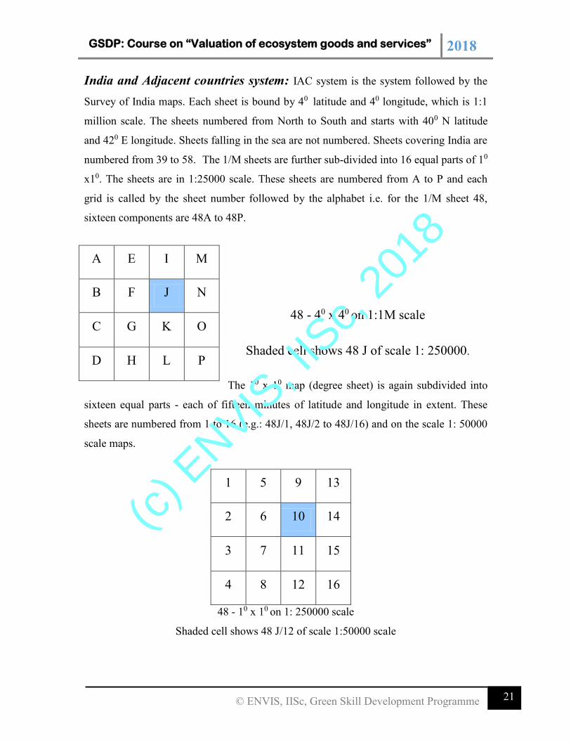
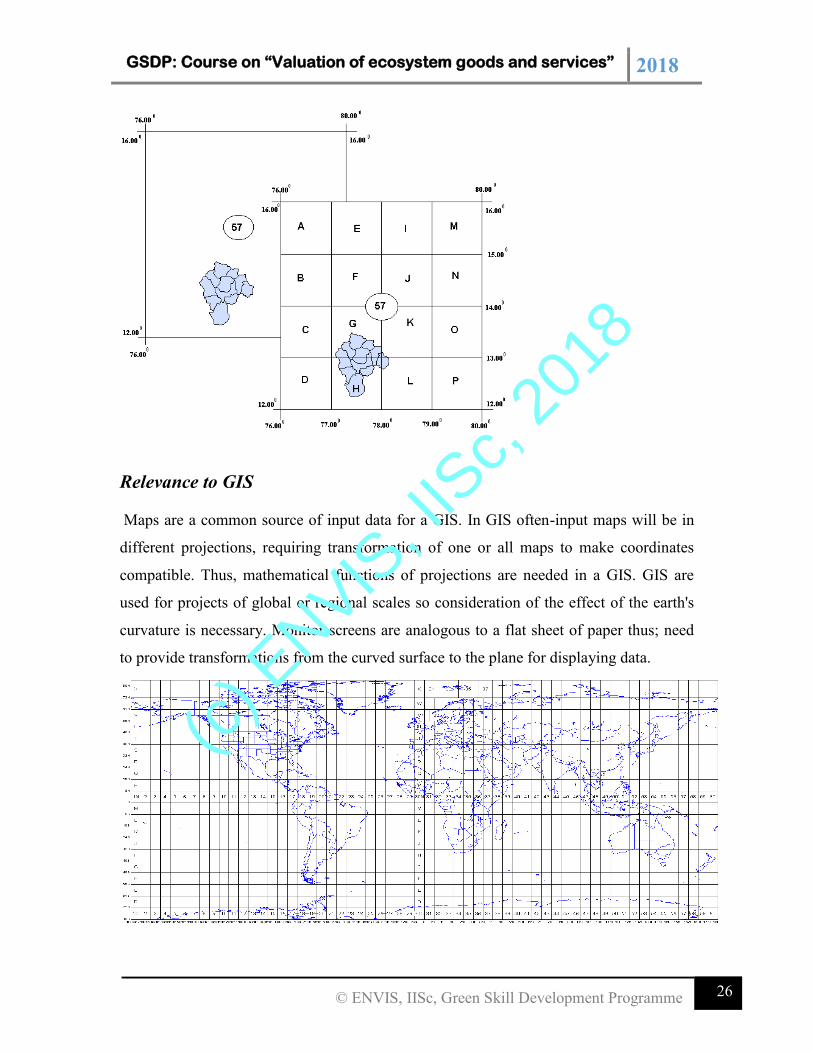
India and Adjacent countries system: IAC system is the system followed by the
Survey of India maps. Each sheet is bound by 40 latitude and 40 longitude, which is 1:1
million scale. The sheets numbered from North to South and starts with 400 N latitude
and 420 E longitude. Sheets falling in the sea are not numbered. Sheets covering India are
numbered from 39 to 58. The 1/M sheets are further sub-divided into 16 equal parts of 10
x10. The sheets are in 1:25000 scale. These sheets are numbered from A to P and each
grid is called by the sheet number followed by the alphabet i.e. for the 1/M sheet 48,
sixteen components are 48A to 48P.
48 - 40 x 40 on 1:1M scale
Shaded cell shows 48 J of scale 1: 250000.
The 10 x 10 map (degree sheet) is again subdivided into
sixteen equal parts - each of fifteen minutes of latitude and longitude in extent. These
sheets are numbered from 1 to 16 (e.g.: 48J/1, 48J/2 to 48J/16) and on the scale 1: 50000
scale maps.
1 5 9 13
2 6 10 14
3 7 11 15
4 8 12 16
48 - 10 x 10 on 1: 250000 scale
Shaded cell shows 48 J/12 of scale 1:50000 scale
A E I M
B F J N
C G K O
D H L P
(c) E
NVIS, I
ISc,
2018
GSDP: Course on “Valuation of ecosystem goods and services” 2018
22 © ENVIS, IISc, Green Skill Development Programme
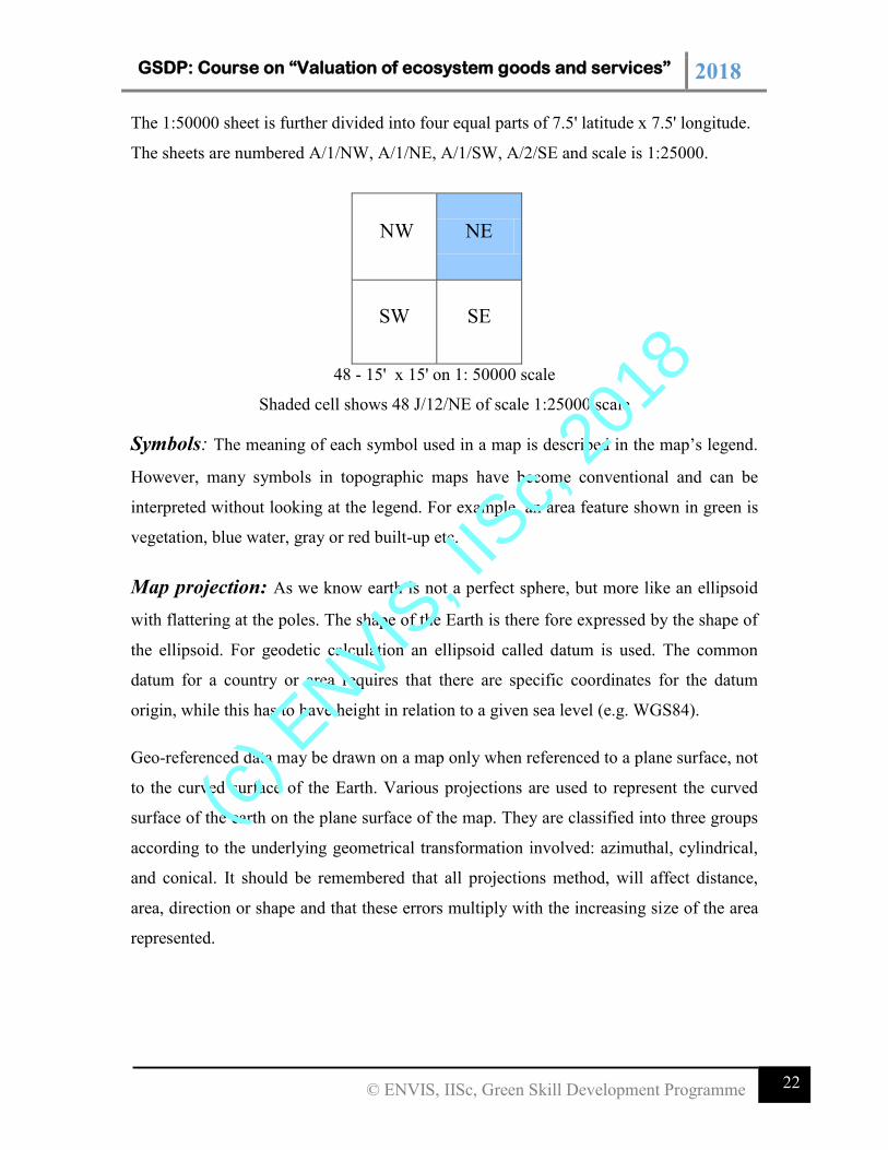
The 1:50000 sheet is further divided into four equal parts of 7.5' latitude x 7.5' longitude.
The sheets are numbered A/1/NW, A/1/NE, A/1/SW, A/2/SE and scale is 1:25000.
NW NE
SW SE
48 - 15' x 15' on 1: 50000 scale
Shaded cell shows 48 J/12/NE of scale 1:25000 scale
Symbols: The meaning of each symbol used in a map is described in the map’s legend.
However, many symbols in topographic maps have become conventional and can be
interpreted without looking at the legend. For example, an area feature shown in green is
vegetation, blue water, gray or red built-up etc.
Map projection: As we know earth is not a perfect sphere, but more like an ellipsoid
with flattering at the poles. The shape of the Earth is there fore expressed by the shape of
the ellipsoid. For geodetic calculation an ellipsoid called datum is used. The common
datum for a country or area requires that there are specific coordinates for the datum
origin, while this has to have height in relation to a given sea level (e.g. WGS84).
Geo-referenced data may be drawn on a map only when referenced to a plane surface, not
to the curved surface of the Earth. Various projections are used to represent the curved
surface of the earth on the plane surface of the map. They are classified into three groups
according to the underlying geometrical transformation involved: azimuthal, cylindrical,
and conical. It should be remembered that all projections method, will affect distance,
area, direction or shape and that these errors multiply with the increasing size of the area
represented.
(c) E
NVIS, I
ISc,
2018
GSDP: Course on “Valuation of ecosystem goods and services” 2018
23 © ENVIS, IISc, Green Skill Development Programme
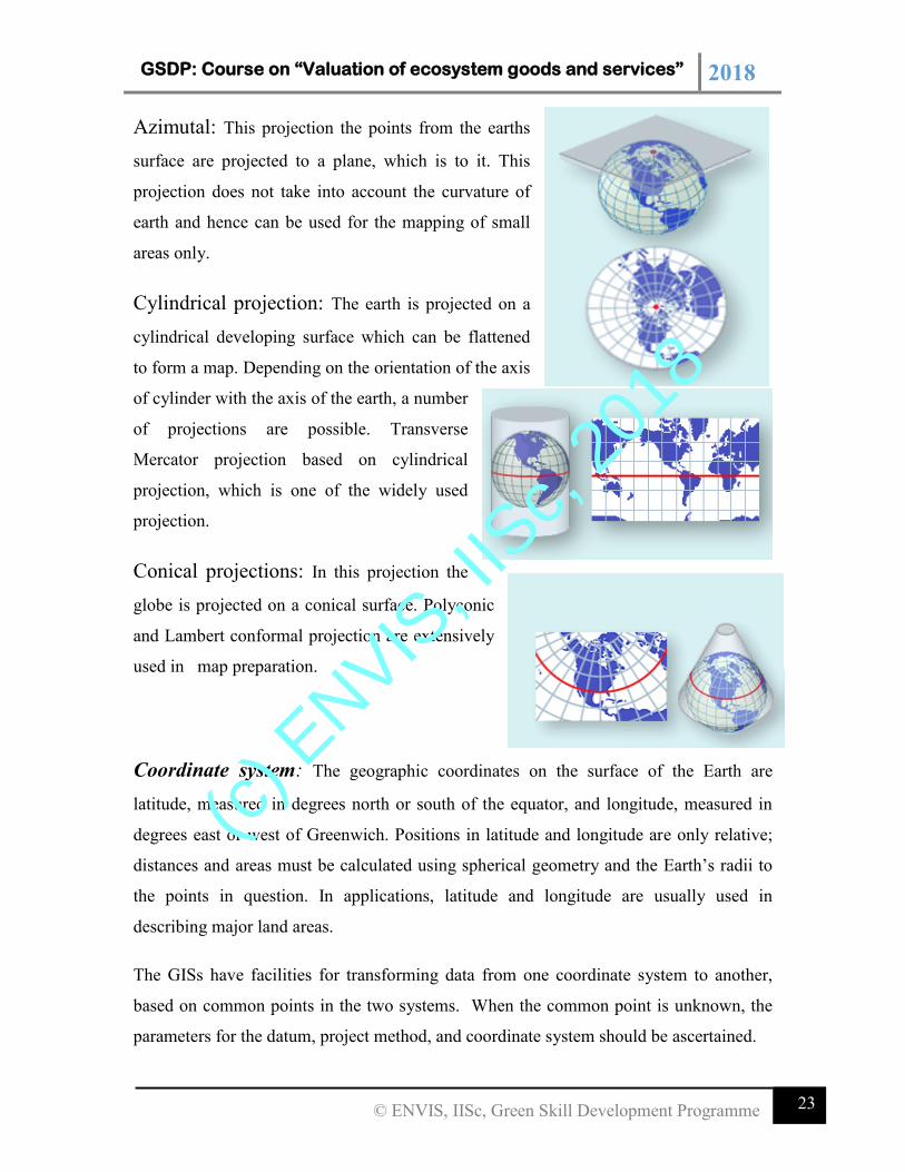
Azimutal: This projection the points from the earths
surface are projected to a plane, which is to it. This
projection does not take into account the curvature of
earth and hence can be used for the mapping of small
areas only.
Cylindrical projection: The earth is projected on a
cylindrical developing surface which can be flattened
to form a map. Depending on the orientation of the axis
of cylinder with the axis of the earth, a number
of projections are possible. Transverse
Mercator projection based on cylindrical
projection, which is one of the widely used
projection.
Conical projections: In this projection the
globe is projected on a conical surface. Polyconic
and Lambert conformal projection are extensively
used in map preparation.
Coordinate system: The geographic coordinates on the surface of the Earth are
latitude, measured in degrees north or south of the equator, and longitude, measured in
degrees east or west of Greenwich. Positions in latitude and longitude are only relative;
distances and areas must be calculated using spherical geometry and the Earth’s radii to
the points in question. In applications, latitude and longitude are usually used in
describing major land areas.
The GISs have facilities for transforming data from one coordinate system to another,
based on common points in the two systems. When the common point is unknown, the
parameters for the datum, project method, and coordinate system should be ascertained.
(c) E
NVIS, I
ISc,
2018
GSDP: Course on “Valuation of ecosystem goods and services” 2018
24 © ENVIS, IISc, Green Skill Development Programme
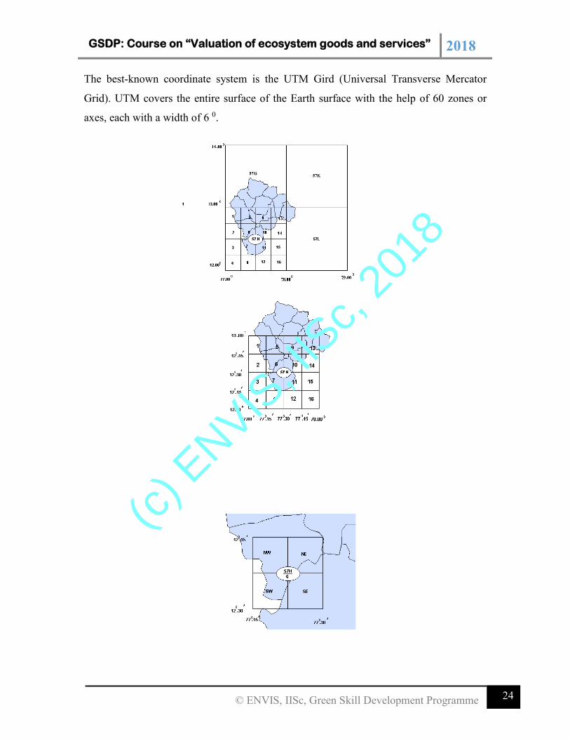
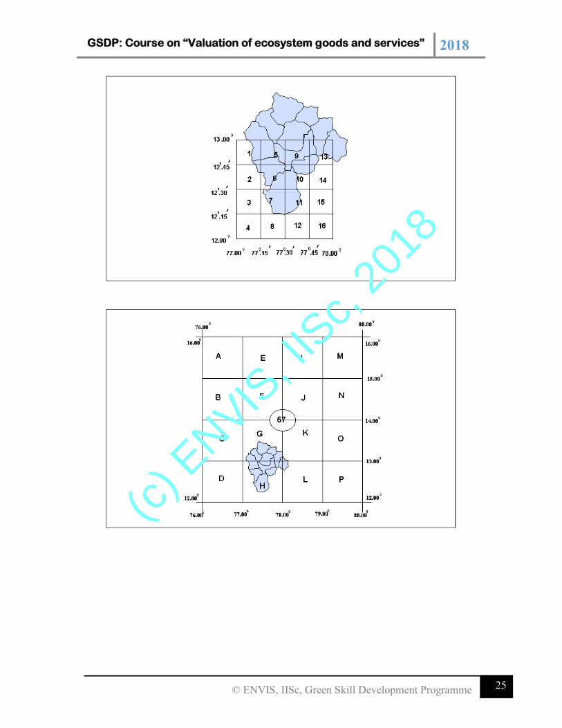
The best-known coordinate system is the UTM Gird (Universal Transverse Mercator
Grid). UTM covers the entire surface of the Earth surface with the help of 60 zones or
axes, each with a width of 6 0.
(c) E
NVIS, I
ISc,
2018
GSDP: Course on “Valuation of ecosystem goods and services” 2018
25 © ENVIS, IISc, Green Skill Development Programme
(c) E
NVIS, I
ISc,
2018
GSDP: Course on “Valuation of ecosystem goods and services” 2018
26 © ENVIS, IISc, Green Skill Development Programme
Relevance to GIS
Maps are a common source of input data for a GIS. In GIS often-input maps will be in
different projections, requiring transformation of one or all maps to make coordinates
compatible. Thus, mathematical functions of projections are needed in a GIS. GIS are
used for projects of global or regional scales so consideration of the effect of the earth's
curvature is necessary. Monitor screens are analogous to a flat sheet of paper thus; need
to provide transformations from the curved surface to the plane for displaying data.
(c) E
NVIS, I
ISc,
2018
GSDP: Course on “Valuation of ecosystem goods and services” 2018
27 © ENVIS, IISc, Green Skill Development Programme
Chapter 3: Introduction to Remote Sensing and Image Processing
Of all the various data sources used in GIS, one of the most important is undoubtedly that
provided by remote sensing. Through the use of satellites, we now have a continuing
program of data acquisition for the entire world with time frames ranging from a couple
of weeks to a matter of hours. Very importantly, we also now have access to remotely
sensed images in digital form, allowing rapid integration of the results of remote sensing
analysis into a GIS
Because of the extreme importance of remote sensing as a data input to GIS, it has
become necessary for GIS analysts (particularly those involved in natural resource
applications) to gain a strong familiarity with Image processing system (IPS).
Consequently, this chapter gives an overview of this important technology and its
integration with GIS.
Definition
Remote sensing can be defined as any process whereby information is gathered about an
object, area or phenomenon without being in contact with it. Our eyes are an excellent
example of a remote sensing device. We are able to gather information about our
surroundings by gauging the amount and nature of the reflectance of visible light energy
from some external source (such as sun or a light bulb) as it reflects off objects in our
field of view. Contrast with this thermometer, which must be in contact with the
phenomenon it measures, and thus is not a remote sensing device.
Given this rather general definition, the term remote sensing has come to be associated
more specifically with the gauging of interactions between earth surface materials and
electromagnetic energy. However, any such attempt at a more specific definition
becomes difficult, since it is not always the natural environment that is sensed (e.g., art
conservation applications), the energy type is not always electromagnetic (e.g., sonar)
and some procedures gauge natural energy emissions (e.g., thermal infrared) rather than
interactions with energy from an independent source.
Basic Process involved-
1. Data Acquisition
2. Data Analysis
(c) E
NVIS, I
ISc,
2018
GSDP: Course on “Valuation of ecosystem goods and services” 2018
28 © ENVIS, IISc, Green Skill Development Programme
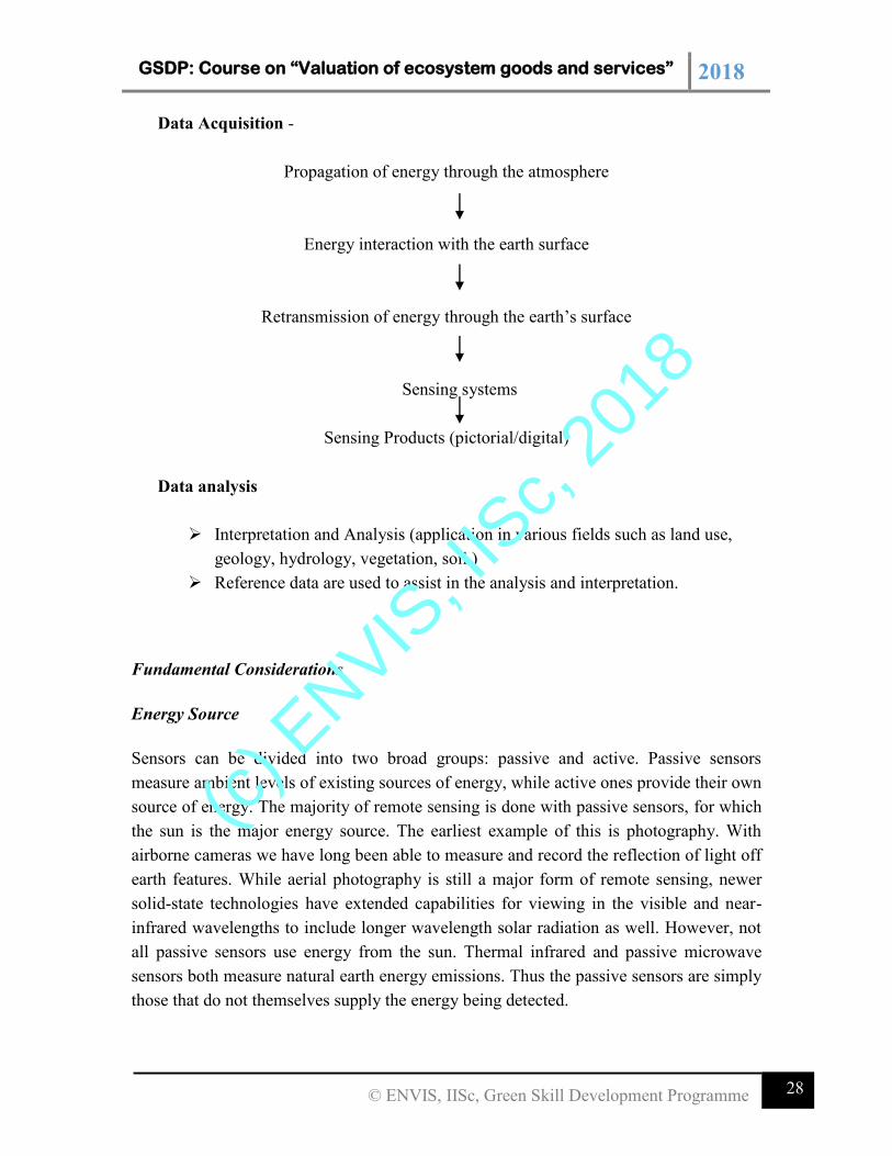
Data Acquisition -
Propagation of energy through the atmosphere
Energy interaction with the earth surface
Retransmission of energy through the earth’s surface
Sensing systems
Sensing Products (pictorial/digital)
Data analysis
Interpretation and Analysis (application in various fields such as land use,
geology, hydrology, vegetation, soil )
Reference data are used to assist in the analysis and interpretation.
Fundamental Considerations
Energy Source
Sensors can be divided into two broad groups: passive and active. Passive sensors
measure ambient levels of existing sources of energy, while active ones provide their own
source of energy. The majority of remote sensing is done with passive sensors, for which
the sun is the major energy source. The earliest example of this is photography. With
airborne cameras we have long been able to measure and record the reflection of light off
earth features. While aerial photography is still a major form of remote sensing, newer
solid-state technologies have extended capabilities for viewing in the visible and near-
infrared wavelengths to include longer wavelength solar radiation as well. However, not
all passive sensors use energy from the sun. Thermal infrared and passive microwave
sensors both measure natural earth energy emissions. Thus the passive sensors are simply
those that do not themselves supply the energy being detected.
(c) E
NVIS, I
ISc,
2018
GSDP: Course on “Valuation of ecosystem goods and services” 2018
29 © ENVIS, IISc, Green Skill Development Programme
By contrast, active sensors provide their own source of energy. The most familiar form of
this is flash photography. However, in environmental and mapping applications, the best
example is RADAR. RADAR systems emit energy in the microwave region of the
electromagnetic spectrum Fig 3.1. This reflection of that energy by earth surface
materials is then measured to produce an image of the area sensed.
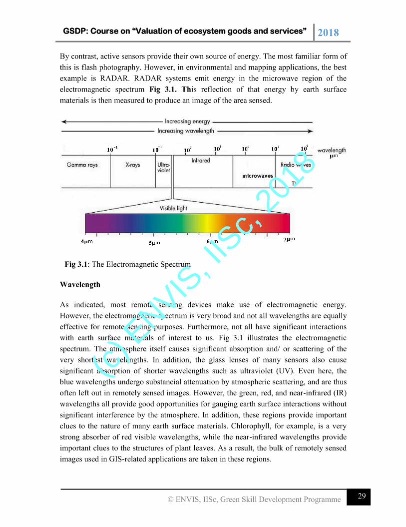
Wavelength
As indicated, most remote sensing devices make use of electromagnetic energy.
However, the electromagnetic spectrum is very broad and not all wavelengths are equally
effective for remote sensing purposes. Furthermore, not all have significant interactions
with earth surface materials of interest to us. Fig 3.1 illustrates the electromagnetic
spectrum. The atmosphere itself causes significant absorption and/ or scattering of the
very shortest wavelengths. In addition, the glass lenses of many sensors also cause
significant absorption of shorter wavelengths such as ultraviolet (UV). Even here, the
blue wavelengths undergo substancial attenuation by atmospheric scattering, and are thus
often left out in remotely sensed images. However, the green, red, and near-infrared (IR)
wavelengths all provide good opportunities for gauging earth surface interactions without
significant interference by the atmosphere. In addition, these regions provide important
clues to the nature of many earth surface materials. Chlorophyll, for example, is a very
strong absorber of red visible wavelengths, while the near-infrared wavelengths provide
important clues to the structures of plant leaves. As a result, the bulk of remotely sensed
images used in GIS-related applications are taken in these regions.
Fig 3.1: The Electromagnetic Spectrum
(c) E
NVIS, I
ISc,
2018
GSDP: Course on “Valuation of ecosystem goods and services” 2018
30 © ENVIS, IISc, Green Skill Development Programme
Extending into the middle and thermal infrared regions, a variety of good windows can
be found. The longer of the middle infrared wavelengths have proven to be useful in a
number of geological applications. The thermal regions have proven to be very useful for
monitoring not only the obvious cases of the spatial distribution of heat from industrial
activity, but a broad set of applications ranging from fire monitoring to animal
distribution studies to soil moisture conditions.
After the thermal IR, the next area of major significance in environmental remote sensing
is in the microwave region. A number of important windows exist in this region and are
of particular importance for the use of active radar imaging. The texture of earth surface
materials causes significant interactions with several of the microwave wavelength
regions. This can thus be used as a supplement to information gained in other
wavelengths, and also offers the significant advantage of being usable at night (because
as an active system it is independent of solar radiation) and in regions of persistent cloud
cover (since radar wavelengths are not significantly affected by clouds).
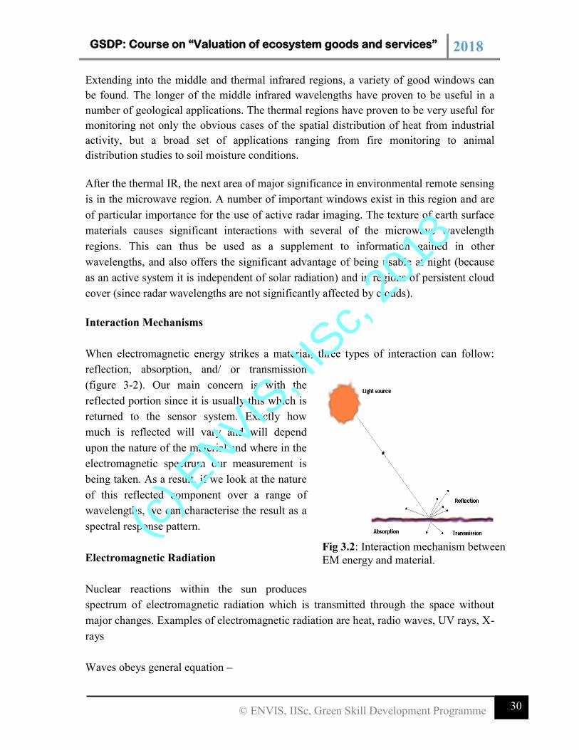
Interaction Mechanisms
When electromagnetic energy strikes a material, three types of interaction can follow:
reflection, absorption, and/ or transmission
(figure 3-2). Our main concern is with the
reflected portion since it is usually this which is
returned to the sensor system. Exactly how
much is reflected will vary and will depend
upon the nature of the material and where in the
electromagnetic spectrum our measurement is
being taken. As a result, if we look at the nature
of this reflected component over a range of
wavelengths, we can characterise the result as a
spectral response pattern.
Electromagnetic Radiation
Nuclear reactions within the sun produces
spectrum of electromagnetic radiation which is transmitted through the space without
major changes. Examples of electromagnetic radiation are heat, radio waves, UV rays, X-
rays
Waves obeys general equation –
Fig 3.2: Interaction mechanism between
EM energy and material.
(c) E
NVIS, I
ISc,
2018
GSDP: Course on “Valuation of ecosystem goods and services” 2018
31 © ENVIS, IISc, Green Skill Development Programme
C = ν x λ
C = 3 x 10⁸ m/s
ν = frequency
λ = wavelength
Wavelength –The distance between one wave crest to the next
Frequency- Number of crests passing a fixed point at a given period of time
Amplitude-Equivalent to height of each peak
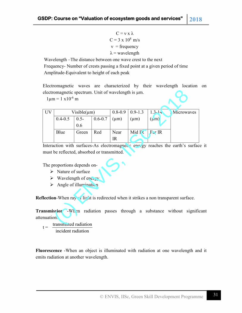
Electromagnetic waves are characterized by their wavelength location on
electromagnetic spectrum. Unit of wavelength is µm.
1µm = 1 x10⁻⁶ m
UV Visible(µm) 0.8-0.9
(µm)
0.9-1.3
(µm)
1.3-14
(µm)
Microwaves
0.4-0.5 0.5-
0.6
0.6-0.7
Blue Green Red Near
IR
Mid IR Far IR
Interaction with surfaces-As electromagnetic energy reaches the earth’s surface it
must be reflected, absorbed or transmitted.
The proportions depends on-
Nature of surface
Wavelength of energy
Angle of illumination
Reflection-When ray of light is redirected when it strikes a non transparent surface.
Transmission -When radiation passes through a substance without significant
attenuation.
t =transmitted radiation
incident radiation
Fluorescence -When an object is illuminated with radiation at one wavelength and it
emits radiation at another wavelength.
(c) E
NVIS, I
ISc,
2018
GSDP: Course on “Valuation of ecosystem goods and services” 2018
32 © ENVIS, IISc, Green Skill Development Programme
Electromagnetic waves are categorized by their wavelength location in
electromagnetic spectrum. Electromagnetic radiation is composed of many discrete
units called photons or quanta.
Q = h ν
Q = energy of quantum, Joules (J)
h = Plank’s constant
ν = Frequency
Q= h (c/ λ)
Q = 1/ λ ie, the longer the wavelength involved the lower is its energy content. All
matter at temperature above absolute zero continuously emits electromagnetic
radiation.
Stefen-Boltzmann Law- The amount of energy a body radiates is the function of its
surface temperature.
M = σ T4
M = total radiant exitance from the surface of a material
σ = Stefen-Boltzmann constant, 5.6697 X 10⁻⁸ Wm-2K-4
T = absolute temperature (K) of the emitting material
Total energy emitted from an object varies as T4 and increase very rapidly as temperature
increases.
The rate at which photons (quanta) strike a surface is called radiant flux (øc ) measured
in Watts.
Irradiance (Ee) is defined as radiant flux per unit area.
A blackbody is a hypothetical source of energy that behaves in an idealized manner. It
absorbs all incident radiation, none of the radiation is reflected.
Kirchoff’s Law states that-The ratio of emitted radiation to the absorbed radiation flux is
same for all black bodies at the same temperature.
Wien’s Displacement law- specifies relationship between wavelength of radiation
emitted and temperature of a black body.
λ = 2897.8 / T
λ = wavelength at which temperature is maximum
T = absolute temperature (K)
(c) E
NVIS, I
ISc,
2018
GSDP: Course on “Valuation of ecosystem goods and services” 2018
33 © ENVIS, IISc, Green Skill Development Programme
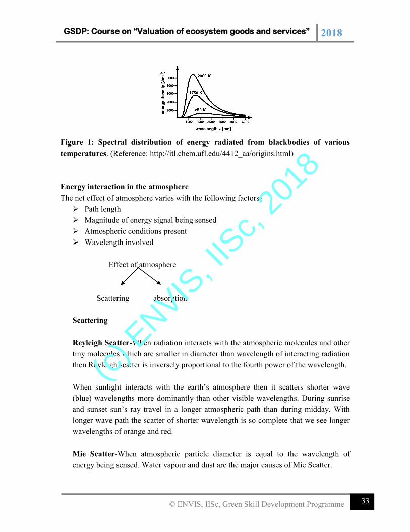
Figure 1: Spectral distribution of energy radiated from blackbodies of various
temperatures. (Reference: http://itl.chem.ufl.edu/4412_aa/origins.html)
Energy interaction in the atmosphere
The net effect of atmosphere varies with the following factors-
Path length
Magnitude of energy signal being sensed
Atmospheric conditions present
Wavelength involved
Effect of atmosphere
Scattering absorption
Scattering
Reyleigh Scatter-When radiation interacts with the atmospheric molecules and other
tiny molecules which are smaller in diameter than wavelength of interacting radiation
then Reyleigh scatter is inversely proportional to the fourth power of the wavelength.
When sunlight interacts with the earth’s atmosphere then it scatters shorter wave
(blue) wavelengths more dominantly than other visible wavelengths. During sunrise
and sunset sun’s ray travel in a longer atmospheric path than during midday. With
longer wave path the scatter of shorter wavelength is so complete that we see longer
wavelengths of orange and red.
Mie Scatter-When atmospheric particle diameter is equal to the wavelength of
energy being sensed. Water vapour and dust are the major causes of Mie Scatter.
(c) E
NVIS, I
ISc,
2018
GSDP: Course on “Valuation of ecosystem goods and services” 2018
34 © ENVIS, IISc, Green Skill Development Programme
Non selective Scatter-When the diameter of particles causing scatter are much larger
than the wavelength of energy being sensed. Water droplets have diameter in the
range 5-100µm and scatters all visible and near to mid IR wavelengths equally. In
visible wavelengths equal quantities of blue, green, red light are scattered hence fog
appears white.
Absorption: Absorption of radiation occurs when atmosphere prevents or strongly
attenuates transmission or radiation of energy through the atmosphere. Water vapour,
carbon di oxide, ozone are the most efficient absorber of solar radiation.
Ozone is formed when oxygen reacts with UV radiation. It lies 20-30 Km in the
stratosphere. Carbon di oxide is important in remote sensing because it is effective in
absorbing radiation in mid and far IR rays. Its strongest absorption occurs in the range
13-17.5µm. Water vapour present in the atmosphere is 0-3% by volume. Two of the
most important regions are several bands between 5.5 to 7.0µm and above
27.0µm.Absorption in these region can exceed 80%if the atmosphere contains
considerable amount of water vapour. The wavelength at which atmosphere is
particularly transmissive of energy are referred as atmospheric windows.
Energy interactions with Earth surface features-
Applying Principle of conservation of Energy, EI (λ) = ER (λ) + EA (λ)+ ET (λ)
EI = incident energy; ER = reflected energy; EA=absorbed energy; ET = transmitted
energy
ER (λ) = EI (λ) - [ EA (λ) + ET (λ)]
Reflected energy is equal to the energy incident on a given feature reduced by the
energy that is either absorbed or transmitted by that feature.
The geometric manner in which an object reflects energy is function of surface
roughness of the object.
Specular reflectors- Flat surface in which angle of reflection is equal to the angle of
incidence.
Diffuse reflectors-rough surface that reflects uniformly in all directions.
(c) E
NVIS, I
ISc,
2018
GSDP: Course on “Valuation of ecosystem goods and services” 2018
35 © ENVIS, IISc, Green Skill Development Programme
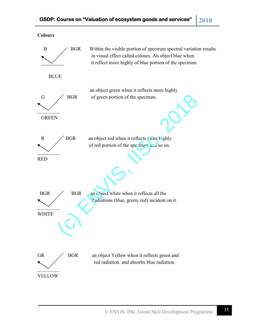
Colours
B BGR Within the visible portion of spectrum spectral variation results
in visual effect called colours. An object blue when
_________ it reflect more highly of blue portion of the spectrum.
BLUE
an object green when it reflects more highly
G BGR of green portion of the spectrum.
_________
GREEN
R BGR an object red when it reflects more highly
of red portion of the spectrum and so on.
_________
RED
BGR BGR an object white when it reflects all the
Radiations (blue, green, red) incident on it.
_________
WHITE
GR BGR an object Yellow when it reflects green and
red radiation and absorbs blue radiation.
_________
YELLOW
(c) E
NVIS, I
ISc,
2018
GSDP: Course on “Valuation of ecosystem goods and services” 2018
36 © ENVIS, IISc, Green Skill Development Programme
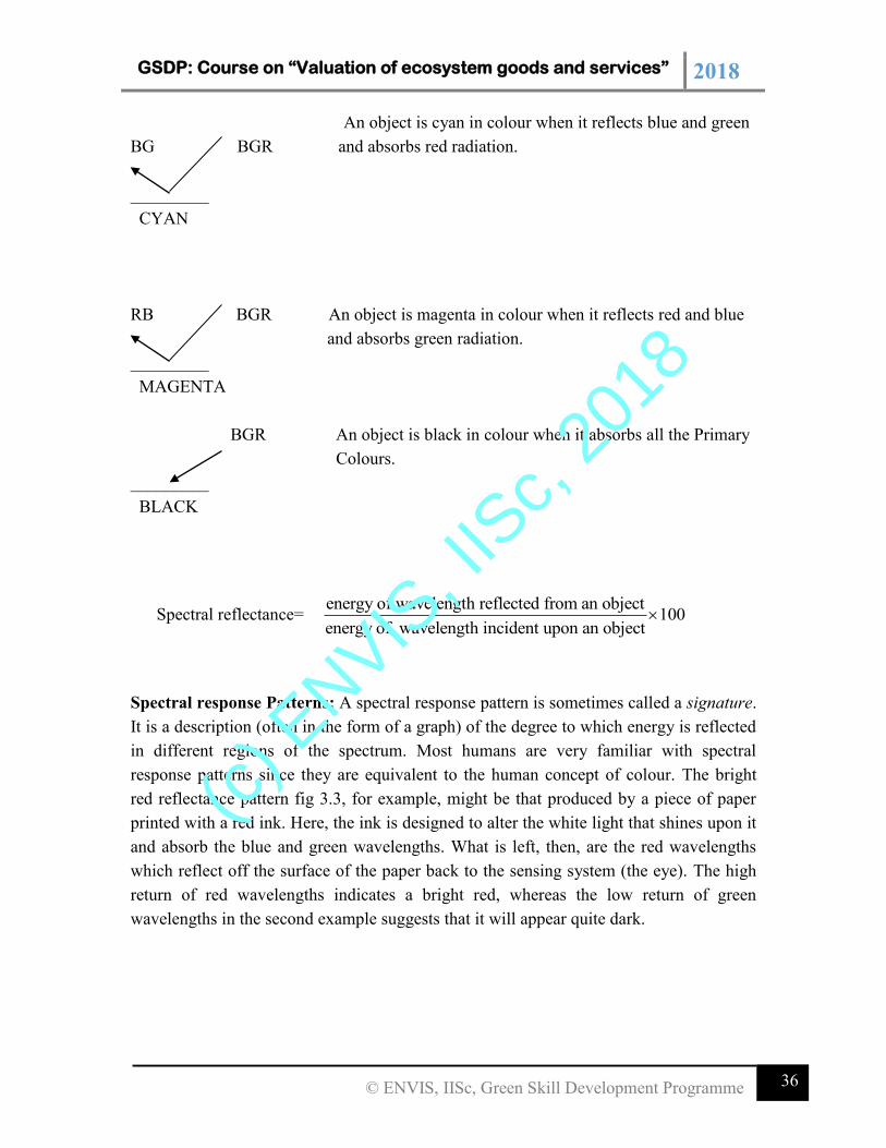
An object is cyan in colour when it reflects blue and green
BG BGR and absorbs red radiation.
_________
CYAN
RB BGR An object is magenta in colour when it reflects red and blue
and absorbs green radiation.
_________
MAGENTA
BGR An object is black in colour when it absorbs all the Primary
Colours.
_________
BLACK
Spectral reflectance= energy of wavelength reflected from an object
100energy of wavelength incident upon an object
Spectral response Patterns: A spectral response pattern is sometimes called a signature.
It is a description (often in the form of a graph) of the degree to which energy is reflected
in different regions of the spectrum. Most humans are very familiar with spectral
response patterns since they are equivalent to the human concept of colour. The bright
red reflectance pattern fig 3.3, for example, might be that produced by a piece of paper
printed with a red ink. Here, the ink is designed to alter the white light that shines upon it
and absorb the blue and green wavelengths. What is left, then, are the red wavelengths
which reflect off the surface of the paper back to the sensing system (the eye). The high
return of red wavelengths indicates a bright red, whereas the low return of green
wavelengths in the second example suggests that it will appear quite dark.
(c) E
NVIS, I
ISc,
2018
GSDP: Course on “Valuation of ecosystem goods and services” 2018
37 © ENVIS, IISc, Green Skill Development Programme
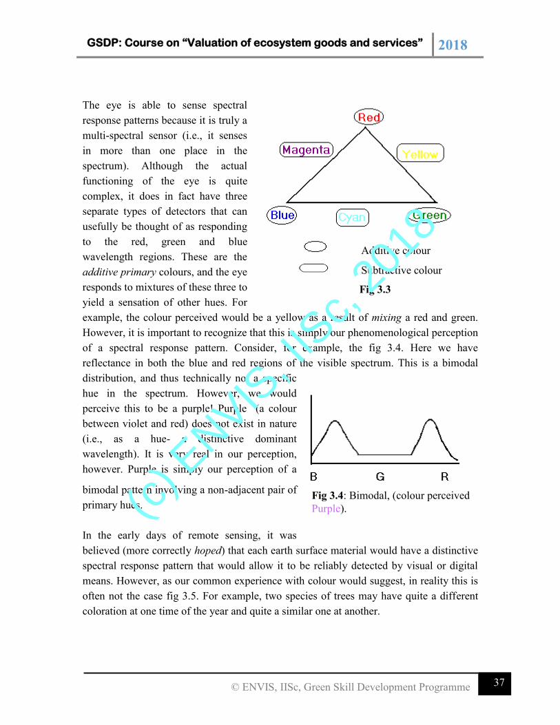
The eye is able to sense spectral
response patterns because it is truly a
multi-spectral sensor (i.e., it senses
in more than one place in the
spectrum). Although the actual
functioning of the eye is quite
complex, it does in fact have three
separate types of detectors that can
usefully be thought of as responding
to the red, green and blue
wavelength regions. These are the
additive primary colours, and the eye
responds to mixtures of these three to
yield a sensation of other hues. For
example, the colour perceived would be a yellow as a result of mixing a red and green.
However, it is important to recognize that this is simply our phenomenological perception
of a spectral response pattern. Consider, for example, the fig 3.4. Here we have
reflectance in both the blue and red regions of the visible spectrum. This is a bimodal
distribution, and thus technically not a specific
hue in the spectrum. However, we would
perceive this to be a purple! Purple (a colour
between violet and red) does not exist in nature
(i.e., as a hue- a distinctive dominant
wavelength). It is very real in our perception,
however. Purple is simply our perception of a
bimodal pattern involving a non-adjacent pair of
primary hues.
In the early days of remote sensing, it was
believed (more correctly hoped) that each earth surface material would have a distinctive
spectral response pattern that would allow it to be reliably detected by visual or digital
means. However, as our common experience with colour would suggest, in reality this is
often not the case fig 3.5. For example, two species of trees may have quite a different
coloration at one time of the year and quite a similar one at another.
Additive colour
Subtractive colour
Fig 3.3
Fig 3.4: Bimodal, (colour perceived
Purple). (c) E
NVIS, I
ISc,
2018
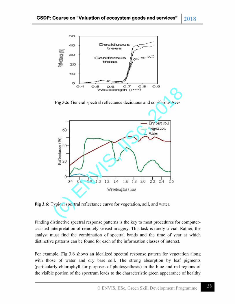
GSDP: Course on “Valuation of ecosystem goods and services” 2018
38 © ENVIS, IISc, Green Skill Development Programme
Fig 3.5: General spectral reflectance deciduous and coniferous trees
Fig 3.6: Typical spectral reflectance curve for vegetation, soil, and water.
Finding distinctive spectral response patterns is the key to most procedures for computer-
assisted interpretation of remotely sensed imagery. This task is rarely trivial. Rather, the
analyst must find the combination of spectral bands and the time of year at which
distinctive patterns can be found for each of the information classes of interest.
For example, Fig 3.6 shows an idealized spectral response pattern for vegetation along
with those of water and dry bare soil. The strong absorption by leaf pigments
(particularly chlorophyll for purposes of photosynthesis) in the blue and red regions of
the visible portion of the spectrum leads to the characteristic green appearance of healthy
(c) E
NVIS, I
ISc,
2018
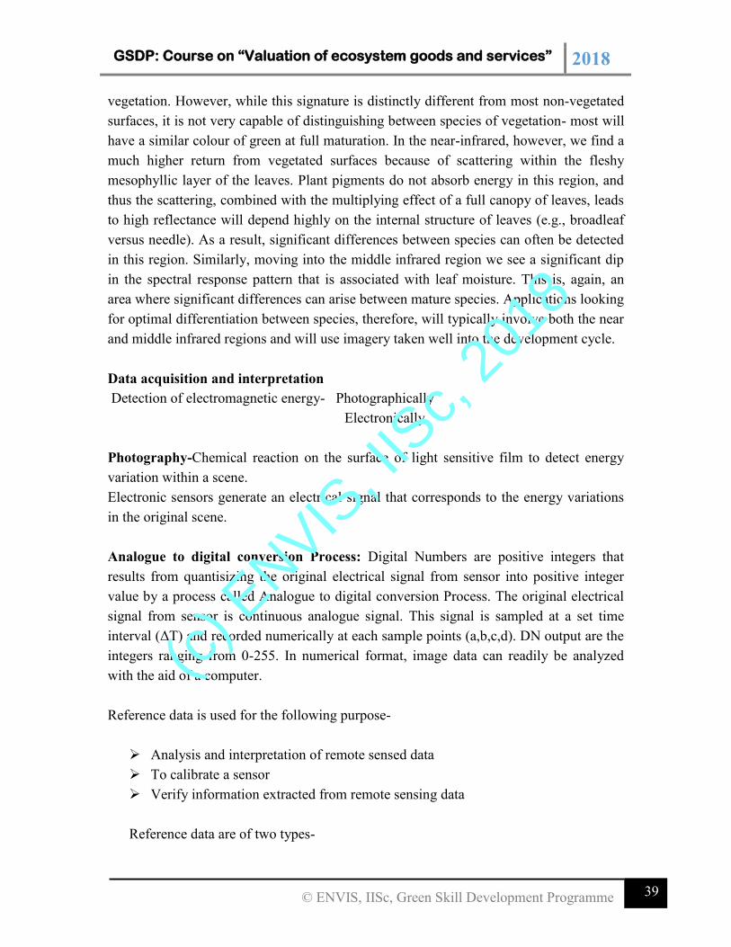
GSDP: Course on “Valuation of ecosystem goods and services” 2018
39 © ENVIS, IISc, Green Skill Development Programme
vegetation. However, while this signature is distinctly different from most non-vegetated
surfaces, it is not very capable of distinguishing between species of vegetation- most will
have a similar colour of green at full maturation. In the near-infrared, however, we find a
much higher return from vegetated surfaces because of scattering within the fleshy
mesophyllic layer of the leaves. Plant pigments do not absorb energy in this region, and
thus the scattering, combined with the multiplying effect of a full canopy of leaves, leads
to high reflectance will depend highly on the internal structure of leaves (e.g., broadleaf
versus needle). As a result, significant differences between species can often be detected
in this region. Similarly, moving into the middle infrared region we see a significant dip
in the spectral response pattern that is associated with leaf moisture. This is, again, an
area where significant differences can arise between mature species. Applications looking
for optimal differentiation between species, therefore, will typically involve both the near
and middle infrared regions and will use imagery taken well into the development cycle.
Data acquisition and interpretation
Detection of electromagnetic energy- Photographically
Electronically
Photography-Chemical reaction on the surface of light sensitive film to detect energy
variation within a scene.
Electronic sensors generate an electrical signal that corresponds to the energy variations
in the original scene.
Analogue to digital conversion Process: Digital Numbers are positive integers that
results from quantisizing the original electrical signal from sensor into positive integer
value by a process called Analogue to digital conversion Process. The original electrical
signal from sensor is continuous analogue signal. This signal is sampled at a set time
interval (ΔT) and recorded numerically at each sample points (a,b,c,d). DN output are the
integers ranging from 0-255. In numerical format, image data can readily be analyzed
with the aid of a computer.
Reference data is used for the following purpose-
Analysis and interpretation of remote sensed data
To calibrate a sensor
Verify information extracted from remote sensing data
Reference data are of two types-
(c) E
NVIS, I
ISc,
2018
GSDP: Course on “Valuation of ecosystem goods and services” 2018
40 © ENVIS, IISc, Green Skill Development Programme
1. Time critical-Where ground conditions changes rapidly with time such as
analysis of vegetation conditions, water pollution events.
2. Time stable-Where materials under observation donot change appreciably with
time such as geologic application.
Spectral Response Pattern- Water and vegetation might reflect equally in visible
light but these features are always separable in IR radiations.
Spectral responses measured by remote sensors over various features permits the
assessment of type and condition of feature and are referred as spectral signatures.
The physical radiation measurement at those wavelengths is referred as spectral
response. Spectral signatures are absolute and unique. Spectral response pattern may
be quantitative but not unique. This variability causes various problems if the
objective is to identify various earth features. Therefore it is important to identify the
nature of ground area one is looking at to minimize spectral variability.
Spectro radiometer- This device measures function of wavelength of the energy coming
from an object within its view.
Bidirectional reflectance Distribution Function –Mathematical description of how
reflectance varies for all combinations of illuminations and viewing angles of a given
wavelength.
Three models of Remote Sensing- The reflection of solar radiation from the earth’s
surface is recorded. Aerial camera mainly uses energy in the visible and near IR portions
of the spectrum.
Passive Remote Sensing - The radiation emitted from the earth’s surface is recorded.
Emitted energy is the strongest in the far IR spectrum. Emitted energy from the earth’s
surface is mainly derived from the short wavelength energy from the sun which is
absorbed by the earth’s surface and reradiated at a longer wavelength. Other sources of
emitted radiations are geothermal energy, heat from steam pipes, power plants.
Active Remote Sensing - Active sensors provide their own energy and therefore they are
independent of terrestrial and solar radiation. Camera with a flash is an example of active
remote sensing.
(c) E
NVIS, I
ISc,
2018
GSDP: Course on “Valuation of ecosystem goods and services” 2018
41 © ENVIS, IISc, Green Skill Development Programme
Ideal Remote sensing system
Uniform energy source
Non-interfering atmosphere-where atmosphere would not modify the energy from
the source in any manner either on the way to the earth surface or coming from it.
Energy matter interaction unique to each and every earth surface.
Super sensor - sensor highly sensitive to all wavelength
A real-time data processing and supply – Each data observation would be
recognized as being unique to the particular terrain element from which it came.
The derived data would provide insight into the physical, chemical and biological
state of each feature of interest.
Photography
Basic concept of camera
Lens to focus light on the film
Light sensitive film to record the object
Shutter that controls the entry of light into camera
Camera body a light tight enclosure
Lens-It gathers light and focuses it on film. The sizes, shapes, arrangement and
composition of lenses are designed to control the bending of light rays to maintain
colour balance and to minimize optical distortions. Imperfection in lens shape
contributes to spherical aberration, a source of error that distorts the image and causes
loss of clarity.
Simple Positive lens- Equal curvature on both the sides. Light rays are refracted from
both the edges to form image.
Compound lens-Formed of separate lenses of varied sizes, shapes and properties.
Optical axis-joins the centre of curvature of both sides of lens.
Image Principle Plane-Plane passing through the centre of lens.
Nodal point-where image principal plane intersects optical axis
Focal Point-Parallel light rays pass through the lens and are brought to the focus at
the focal point.
(c) E
NVIS, I
ISc,
2018
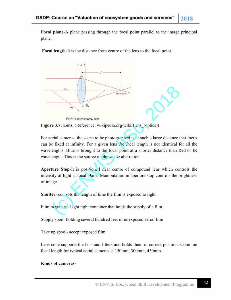
GSDP: Course on “Valuation of ecosystem goods and services” 2018
42 © ENVIS, IISc, Green Skill Development Programme
Focal plane-A plane passing through the focal point parallel to the image principal
plane.
Focal length-It is the distance from centre of the lens to the focal point.
Figure 3.7: Lens. (Reference: wikipedia.org/wiki/Lens_(optics))
For aerial cameras, the scene to be photographed is at such a large distance that focus
can be fixed at infinity. For a given lens the focal length is not identical for all the
wavelengths. Blue is brought to the focal point at a shorter distance than Red or IR
wavelength. This is the source of chromatic aberration.
Aperture Stop-It is positioned near centre of compound lens which controls the
intensity of light at focal plane. Manipulation in aperture stop controls the brightness
of image.
Shutter- controls the length of time the film is exposed to light.
Film magazine-Light tight container that holds the supply of a film.
Supply spool-holding several hundred feet of unexposed aerial film
Take up spool- accept exposed film
Lens cone-supports the lens and filters and holds them in correct position. Common
focal length for typical aerial cameras is 150mm, 300mm, 450mm.
Kinds of cameras-
(c) E
NVIS, I
ISc,
2018
GSDP: Course on “Valuation of ecosystem goods and services” 2018
43 © ENVIS, IISc, Green Skill Development Programme
Reconnaissance camera
Military use
Donot have geometric accuracy
Ability to take photograph at high speed
Ability to take photograph in unfavourable light conditions and low speed
Strip camera
It acquires images by moving film past a fixed slit that serves as shutter.
The speed of the film movement as it passes through the shutter is coordinated
with the speed of aircraft movement.
High quality image from planes flying at high speed and low altitude.
Panoramic cameras
It is designed to record a very wide field of view.
Photograph from panoramic camera show a narrow strip of terrain that is
perpendicular to the flight track from horizon to horizon.
Serious geometric distortions
Useful for large area they represents
Black and white aerial Films
Major components
Base- a thin (40-100µm), flexible transparent material that holds a light sensitive coating
(photographic emulsion).
Emulsion-Modern emulsion consists of Silver halide (silver bromide-95% and silver
iodide-5%).
Silver halide crystals are insoluble and donot adhere to the base. Silver halide crystals are
hold in suspension by gelatin and are evenly spread. Gelatin is transparent, porous and
absorbs light rays when light strikes the emulsion.
Physical properties of Silver halide-
Extremely small
irregular in shape
sharp edges
The finer the size of the grain the finer details can be recorded. Below the emulsion is
subbing layer to ensure that it adhere to the base. On the reverse side of the base there is
(c) E
NVIS, I
ISc,
2018
GSDP: Course on “Valuation of ecosystem goods and services” 2018
44 © ENVIS, IISc, Green Skill Development Programme
antihalation backing that absorbs light that passes through the emulsion and the base and
prevents reflection back to the emulsion.
Process-When the shutter opens it allows the light to enter and strike the emulsion .Silver
halide crystals are very small and even a small area of a film contains thousands of
crystals. When light strikes a crystal then it converts small portion of crystals into
metallic silver. The more intense the light striking a portion of the film the greater is the
number of crystals affected.
Development-The process of bathing the exposed film in an alkaline chemical developer
that reduces the silver halide grain that exposed to the light. Fixer is applied to dissolve or
remove unexposed silver halide grains. After development and fixing the resulting image
is a negative representation of a scene. Those areas which were brightest in the scene are
represented by greatest concentration of metallic silver. Film speed is the measure of
sensitivity of light. A fast film requires low intensity of light for proper exposure, slow
film requires more amount of light.
Contrast-It represents a range of gray tones recorded in the film. High contrast means a
scene largely in black and white with few gray tones. Low contrast indicates
representation of largely gray tones with less dark and bright tones.
Spectral sensitivity records the spectral region to which a film is sensitive.
Panchromatic film-emulsion that is sensitive to radiation throughout visible spectrum.
Orthochromatic film-films with preferred sensitivity in blue and green usually with
peak sensitivity in the green region.
Black and white infrared film- deep red filter that blocks visible radiation but allows IR
rays to pass. Living vegetation appears many times brighter in near IR portion of
spectrum.
Characteristic curve
When the original scene is bright then the negative has large amount of silver that creates
dark area. Where the original scene is dark the film is clear with shades of gray due to
variations in the abundance of crystals present in the film.
(c) E
NVIS, I
ISc,
2018
GSDP: Course on “Valuation of ecosystem goods and services” 2018
45 © ENVIS, IISc, Green Skill Development Programme
When light of intensity is passed through a portion of negative the brightness of light
measured on the other side is a measure of darkness of that region of the film.
Darkness of the film is related to the brightness of the original scene.
E = i x t
E = effect of light upon emulsion
i=intensity
t =time
Colour reversal films
Films coated with three separate emulsions each sensitive to one of the three additive
primaries. The layer between upper most blue sensitive emulsion and middle green
sensitive emulsion is treated to act as yellow filter to prevent the blue light from passing
through the upper layers. This filter is necessary as it is difficult to manufacture
emulsions which are sensitive to red and green light without sensitizing them to blue
light.
Upon exposure blue light passes through the blue layer and exposes it. Yellow
filter prevents the blue light from exposing the green sensitive emulsion and red
sensitive emulsion.
Green light passes through the blue layer and exposes the green sensitive
emulsion.
Red light passes through the emulsions to expose the red sensitive emulsion.
After Processing-
The areas which are not exposed to blue light on blue sensitive emulsion are
represented by yellow dye and those which are exposed to blue are left clear.
The areas which are not exposed to green light on green sensitive emulsion are
represented by magenta dye and those which are exposed to green are left clear.
The areas which are not exposed to red light on red sensitive emulsion are
represented by cyan dye and those which are exposed to red are left clear.
When the processed film is viewed as a transparency against a light source-
Magenta and cyan dye combines to form blue colour.
Yellow and cyan dye combines to give green colour.
Yellow and magenta dye combines to give red colour.
(c) E
NVIS, I
ISc,
2018
GSDP: Course on “Valuation of ecosystem goods and services” 2018
46 © ENVIS, IISc, Green Skill Development Programme
Colour IR Films-
Yellow filter is present to prevent blue light from entering the camera. Blue sensitive
layer is represented by a layer which is sensitive to a portion of near IR. After developing
representation of colour is shifted one position in the spectrum. Green in the scene
appears blue in the image, red appears green and objects representing near IR is depicted
red.
Objects in the scene reflects blue green red IR
Colour reversal films represents object as blue green red IR
Colour IR films represents object as blue green red
Green light exposes the green sensitive layer, red light expose the red sensitive layer and
IR radiation exposes the IR sensitive layer.
After Processing-
The areas which are not exposed to green light are represented by yellow dye.
The areas which are not exposed to red light are represented by magenta dye.
The areas which are not exposed to IR radiation are represented by cyan dye.
In the final transparency-
Magenta and cyan dye combine to form blue colour (green area as blue)
Yellow and cyan dye combine to give green colour ( red area as green)
Yellow and magenta dye combine to give red colour (near IR)
Geometry of Vertical aerial Photograph-
Oblique aerial Photograph-Cameras are oriented towards the side of the aircraft.
Vertical Photograph-Camera directly aimed at the earth’s surface.
Image Acquisition
Fiducial Marks - appear at edges and corners of Photographs
Principal Point-The lines that connects the opposite pairs of fiducial mark intersects at
one point called Principal Point.
Ground nadir-The point on the ground vertically beneath the centre of camera lens at the
time photograph was taken.
(c) E
NVIS, I
ISc,
2018
GSDP: Course on “Valuation of ecosystem goods and services” 2018
47 © ENVIS, IISc, Green Skill Development Programme
Photographic nadir - Intersection of the photograph of vertical line that intersects the
ground nadir and centre of the lens.
Relief displacement-Positional error in vertical aerial Photography
Amount of displacement depends upon-
Height of object
Distance of object from nadir
Optical distortion-error caused by inferior camera lens
Tilt- Displacement of focal length from truly horizontal position due to aircraft motion.
Coverage of Multiple Photographs-
Vertical aerial photographs are obtained by a series of parallel flight lines to get complete
coverage of specific region. When it is necessary to photograph large areas, coverage is
build by several strips of photography called flight line.
Stereoscopic Parallex-
Difference in the appearance of an object due to change in perspective.
The amount of parallex decreases as the distance increases between the source
and the observer.
Displacement due to stereo parallex is always parallel to the flight lines.
Tops of tall objects nearer to the camera show more displacement than shorter
objects which are more distant from camera.
Mosaics- A series of vertical photographs that shows adjacent regions on the ground
can be joined together to form mosaics
Uncontrolled mosaic-Photographs are placed together in a manner that gives
continuous coverage of an area without concern for its preservation of consistent scale
and positional relationships by simply placing the photograph in the correct sequence
Controlled mosaic-Individual photographs arranged in a manner that preserves its
positional relationship with the feature they represents.
Orthophotos -shows photographic details without error caused by tilt and relief
displacement.
Orthophotomap – preserve consistent scale throughout the image without
geometrical error.
(c) E
NVIS, I
ISc,
2018
GSDP: Course on “Valuation of ecosystem goods and services” 2018
48 © ENVIS, IISc, Green Skill Development Programme
Multispectral Remote Sensing
In the visual interpretation of remotely sensed images, a variety of image characteristics
are brought into consideration: colour (or tone in the case of panchromatic images),
texture, size, shape, pattern, context, and the like. However, with computer-assisted
interpretation, it is most often simply colour (i.e., the spectral response pattern) that is
used. It is for this reason that a strong emphasis is placed on the use of multispectral
sensors (sensors that, like the eye, look at more than one place in the spectrum and thus
are able to gauge spectral response patterns), and the number and specific placement of
these spectral bands.
It can be shown through analytical techniques such as Principal Components Analysis,
that in many environments, the bands that carry the greatest amount of information about
the natural environment are the near-infrared and red wavelength bands. Water is
strongly absorbed by infrared wavelengths and is thus highly distinctive in that region. In
addition, plant species typically show their greatest differentiation here. The red area also
very important because it is the primary region in which chlorophyll absorbs energy for
photosynthesis. Thus it is this band which can most readily distinguish between vegetated
and non-vegetated surfaces.
Given this importance of the red and near-infrared bands, it is not surprising that sensor
systems designed for earth resource monitoring will invariably include these in any
particular multi-spectral system. Other bands will depend upon the range of applications
envisioned. Many include the green visible band since it can be used, along with the other
two, to produce a traditional false colour composite - a full colour image derived from the
green, red, and infrared bands (as opposed to the blue, green, and red bands of natural
colour images). This format became common with the advent of colour infrared
photography, and is familiar to many specialists in the remote sensing field. In addition,
the combination of these three bands works well in the interpretation of the cultural
landscape as well as natural and vegetated surfaces. However, it is increasingly common
to include other bands that are more specifically targeted to the differentiation of surface
materials.
Hyper spectral remote Sensing: In addition to traditional multispectral imagery, some
new and experimental systems such as AVIRIS and MODIS are capable of capturing
hyperspectral data. These systems cover a similar wavelength range to multispectral
systems, but in much narrower bands. This dramatically increases the number of bands
(c) E
NVIS, I
ISc,
2018
GSDP: Course on “Valuation of ecosystem goods and services” 2018
49 © ENVIS, IISc, Green Skill Development Programme
(and thus precision) available for image classification (typically tens and even hundreds
of very narrow bands). Moreover, hyperspectral signature libraries have been created in
lab conditions and contain hundreds of signatures for different types of landcovers,
including many materials and other earth materials. Thus, it should be possible to match
signatures to surface materials with great precision. However, environmental conditions
and natural variations in materials (which make them different from standard library
materials) make this difficult. In addition, classification procedures have not been
developed for hyperspectral data to the degree they have been for multispectral imagery.
As a consequence, multispectral imagery still represents the major tool of remote sensing
today.
Some Operational Earth Observation Systems
The systems are grouped into following categories-
Low resolution system with spatial resolution 1Km-5Km.
Medium resolution system with spatial resolution between 10m-100m.
High resolution system with spatial resolution better than 10m.
Imaging spectrometric systems with high spectral resolution.
Table 1: Evolution of various satellites.
S.No Satellite Sensor Temporal
resolution
Spectral
resolution
Spatial
resolution
1. NOAA-17
National
Oceanic and
Atmospheric
Administration
AVHRR-3
Advanced Very
High Resolution
Radiometer
2-14 times
per day
0.58-0.68(1),
0.73-1.00(2),
1.58-1.64
(3A day)
3.55 -3.93
(3B night)
10.3-11.3(4)
11.5-12.5(5)
1 Km X 1Km
(at nadir)
6 Km X 2Km
(at limb)
2. Landsat MSS
Multispectral
scanner
18 days 0.5-0.6
0.6-0.7
0.7-0.8
0.8-1.1
79/82m
79/82m
79/82m
79/82m
79/82m
TM
The Thematic
Mapper
18 days 0.45-0.52(1)
0.52-0.60(2)
0.63-0.69(3)
0.76-0.90(4)
30m
30m
30m
30m
(c) E
NVIS, I
ISc,
2018
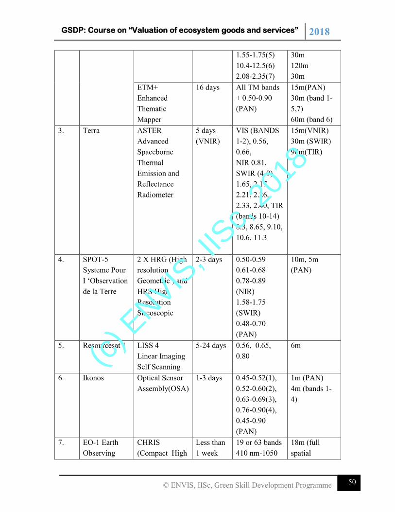
GSDP: Course on “Valuation of ecosystem goods and services” 2018
50 © ENVIS, IISc, Green Skill Development Programme
1.55-1.75(5)
10.4-12.5(6)
2.08-2.35(7)
30m
120m
30m
ETM+
Enhanced
Thematic
Mapper
16 days All TM bands
+ 0.50-0.90
(PAN)
15m(PAN)
30m (band 1-
5,7)
60m (band 6)
3. Terra ASTER
Advanced
Spaceborne
Thermal
Emission and
Reflectance
Radiometer
5 days
(VNIR)
VIS (BANDS
1-2), 0.56,
0.66,
NIR 0.81,
SWIR (4-9),
1.65, 2.17,
2.21, 2.26,
2.33, 2.40, TIR
(bands 10-14)
8.3, 8.65, 9.10,
10.6, 11.3
15m(VNIR)
30m (SWIR)
90m(TIR)
4. SPOT-5
Systeme Pour
I ‘Observation
de la Terre
2 X HRG (High
resolution
Geometric ) and
HRS High
Resolution
Streoscopic
2-3 days 0.50-0.59
0.61-0.68
0.78-0.89
(NIR)
1.58-1.75
(SWIR)
0.48-0.70
(PAN)
10m, 5m
(PAN)
5. Resourcesat 1 LISS 4
Linear Imaging
Self Scanning
5-24 days 0.56, 0.65,
0.80
6m
6. Ikonos Optical Sensor
Assembly(OSA)
1-3 days 0.45-0.52(1),
0.52-0.60(2),
0.63-0.69(3),
0.76-0.90(4),
0.45-0.90
(PAN)
1m (PAN)
4m (bands 1-
4)
7. EO-1 Earth
Observing
CHRIS
(Compact High
Less than
1 week
19 or 63 bands
410 nm-1050
18m (full
spatial
(c) E
NVIS, I
ISc,
2018
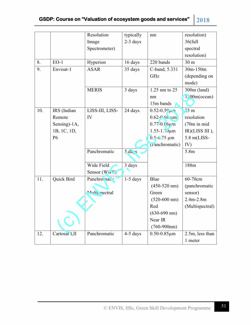
GSDP: Course on “Valuation of ecosystem goods and services” 2018
51 © ENVIS, IISc, Green Skill Development Programme
Resolution
Image
Spectrometer)
typically
2-3 days
nm resolution)
36(full
spectral
resolution)
8. EO-1 Hyperion 16 days 220 bands 30 m
9. Envisat-1 ASAR 35 days C-band, 5.331
GHz
30m-150m
(depending on
mode)
MERIS 3 days 1.25 nm to 25
nm
15m bands
300m (land)
1200m(ocean)
10. IRS (Indian
Remote
Sensing)-1A,
1B, 1C, 1D,
P6
LISS-III, LISS-
IV
24 days 0.52-0.59µm
0.62-0.68 µm
0.77-0.86µm
1.55-1.70µm
0.5-0.75 µm
(Panchromatic)
23 m
resolution
(70m in mid
IR)(LISS III ),
5.8 m(LISS-
IV)
Panchromatic
5 days 5.8m
Wide Field
Sensor (WiFS)
3 days 188m
11. Quick Bird Panchromatic
Multispectral
1-5 days Blue
(450-520 nm)
Green
(520-600 nm)
Red
(630-690 nm)
Near IR
(760-900nm)
60-70cm
(panchromatic
sensor)
2.4m-2.8m
(Multispectral)
12. Cartosat I,II Panchromatic
4-5 days 0.50-0.85µm 2.5m, less than
1 meter
(c) E
NVIS, I
ISc,
2018
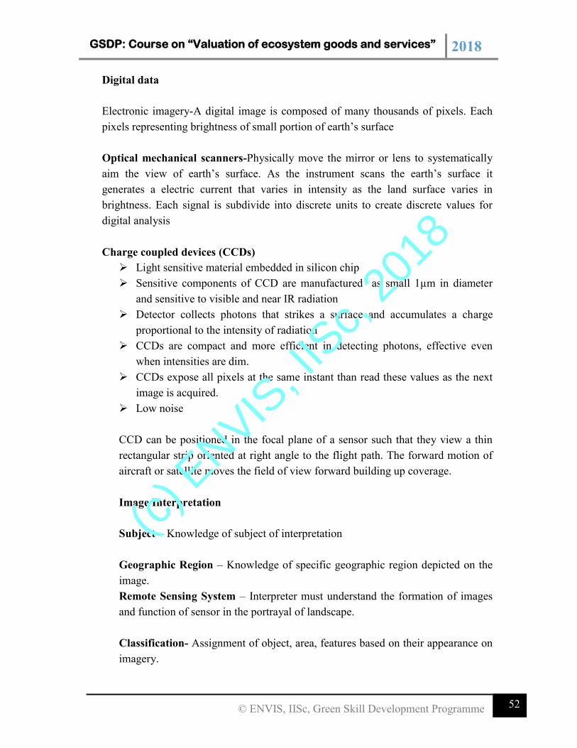
GSDP: Course on “Valuation of ecosystem goods and services” 2018
52 © ENVIS, IISc, Green Skill Development Programme
Digital data
Electronic imagery-A digital image is composed of many thousands of pixels. Each
pixels representing brightness of small portion of earth’s surface
Optical mechanical scanners-Physically move the mirror or lens to systematically
aim the view of earth’s surface. As the instrument scans the earth’s surface it
generates a electric current that varies in intensity as the land surface varies in
brightness. Each signal is subdivide into discrete units to create discrete values for
digital analysis
Charge coupled devices (CCDs)
Light sensitive material embedded in silicon chip
Sensitive components of CCD are manufactured as small 1µm in diameter
and sensitive to visible and near IR radiation
Detector collects photons that strikes a surface and accumulates a charge
proportional to the intensity of radiation
CCDs are compact and more efficient in detecting photons, effective even
when intensities are dim.
CCDs expose all pixels at the same instant than read these values as the next
image is acquired.
Low noise
CCD can be positioned in the focal plane of a sensor such that they view a thin
rectangular strip oriented at right angle to the flight path. The forward motion of
aircraft or satellite moves the field of view forward building up coverage.
Image Interpretation
Subject – Knowledge of subject of interpretation
Geographic Region – Knowledge of specific geographic region depicted on the
image.
Remote Sensing System – Interpreter must understand the formation of images
and function of sensor in the portrayal of landscape.
Classification- Assignment of object, area, features based on their appearance on
imagery.
(c) E
NVIS, I
ISc,
2018
GSDP: Course on “Valuation of ecosystem goods and services” 2018
53 © ENVIS, IISc, Green Skill Development Programme
Detection – Determination of presence or absence of a feature
Recognition – Higher level of knowledge about a feature
Identification – Identity of a given feature can be specified with enough
confidence.
Enumeration- Task of listing or counting discrete items present on an image.
Measurement -
Measurement of distance and height
Extension of volumes and areas as well.
Delineation –
Interpreter must delineate or outline regions as observed on remotely sensed
data.
Interpreter must be able to separate distinct areal units characterized by
specific tones and textures.
Identify edges or boundaries between separate areas.
Elements of Image interpretation
Image tone- denotes lightness or darkness of a region within an image
For black and white images – tones may be characterized by light, medium gray,
dark gray.
For colour images- tones simply refers to colours. Image tone refers ultimately to the
brightness of an area of the ground.
Hue refers to the colour on the image as defined in the intensity-hue –saturation
(IHS).
Tonal variations are an important interpretation element in an image
interpretation.
The tonal expression of object on the image is directly related to the amount of
light reflected from its surface.
Different types of rock, soil or vegetation most likely have different tones.
(c) E
NVIS, I
ISc,
2018
GSDP: Course on “Valuation of ecosystem goods and services” 2018
54 © ENVIS, IISc, Green Skill Development Programme
Image texture- Apparent roughness or smoothness of an image.
Usually image texture is caused by pattern of highlighted and shadowed area
created when an irregular surface is illuminated with an oblique angle.
Image texture depends on the surface and the angle of illumination.
Shadow
Provides an important clue
Features illuminated at an angle cast a shadow that reveal characteristic of its
shape and size.
Military photo interpreters have developed techniques to use shadows to
distinguish subtle difference that might not show otherwise.
Useful in identification of man-made landscape
Pattern
Arrangement of individual objects into distinctive recurring form that
facilitate the recognition.
Pattern can be described by terms such as concentric, radial, checkerboard,
etc.
Some land uses however have specific and characteristic pattern when
observed from on aerospace data.
Examples include the hydrological system rivers with its branches and
patterns related to erosion.
Association
When identification of a specific class of equipment implies that other more
important items are likely to be found nearby.
An example of association is an interpretation of a thermal power plant based
on the combined recognition of high chimneys, large buildings, cooling
towers, coal heaps etc.
Shape
Obvious clues of their identity
Individual structures have characteristic shapes.
Height differences are important to distinguish between different vegetation
types and also in geomorphological mapping. The shape of objects often helps
to determine the character of the object (build up, roads and railways
agricultural fields etc.).
(c) E
NVIS, I
ISc,
2018
GSDP: Course on “Valuation of ecosystem goods and services” 2018
55 © ENVIS, IISc, Green Skill Development Programme
Size
Relative size of the other object in relation to the other objects on the image
provides the interpreter with the notion of its scale and resolution.
Accurate measurement can be valuable as interpretation aid.
The width of road can be estimated by comparing it to the size of the cars,
which is generally known. Subsequently this width determine the road type,
e.g. primary road, secondary road etc.
Site
Refers to topological positions
Sewage treatment facility is positioned near low topological sites near the
steams or rivers to collect the waste water flowing from high location.
A typical example of this interpolation element is that back swamps can be
found in a flood plain but not in the centre of city area.
The global positioning system (GPS)
The Global Positioning System (GPS) is a location system based on a constellation of 24
satellites orbiting the earth at altitudes of approximately 20,200 kilometres. GPS satellites
are orbited high enough to avoid the problems associated with land based systems, yet
can provide accurate positioning 24 hours a day, anywhere in the world. Uncorrected
positions determined from GPS satellite signals produce accuracies in the range 100
meters. When using a technique called differential correction, users can get positions
accurate to within 5 meters or less. With some consideration for error, GPS can provide
any point on earth with a unique address (its precise location). A GIS is a descriptive
database of the earth (or a specific part of the earth). GPS provide location of a point (X,
Y, Z), while GIS gives the information at that location.
GPS is most useful for:
Locating new survey control stations and up grading the accuracy of the old
station
Measuring terrain features that are difficult to measure by conventional means
Positioning of offshore oil platforms
(c) E
NVIS, I
ISc,
2018
GSDP: Course on “Valuation of ecosystem goods and services” 2018
56 © ENVIS, IISc, Green Skill Development Programme
Updating road data with a GPS receiver in the vehicle
Marine navigation, including integration with electronic charts
Determining camera- carrying aircraft positions to reduce reliance on fixed marks
in aerial photography
Determination of difference in elevation.
GPS/GIS is reshaping the way users locate, organise, analyse and map the resources.
Successful application of remote sensing:
Evaluation for the potential for addressing the problem with remote
sensing techniques.
Identification of remote sensing data acquisition procedures appropriate
to the task.
Determination of data interpretation procedures to be employed and the
reference data needed.
Identification of the criteria by which the quality of information collected
can be judged.
Clear definition of problem at hand
Evaluation for the potential for addressing the problem with remote
sensing techniques.
Identification of remote sensing data acquisition procedures appropriate
to the task.
Determination of data interpretation procedures to be employed and the
reference data needed.
Identification of the criteria by which the quality of information collected
can be judged.
(c) E
NVIS, I
ISc,
2018
GSDP: Course on “Valuation of ecosystem goods and services” 2018
57 © ENVIS, IISc, Green Skill Development Programme
DIGITAL IMAGE PROCESSING.
As a result of solid state multispectral scanners and other raster input devices, we now
have available digital raster images of spectral reflectance data. The chief advantage of
having these data in digital form is that they allow us to apply computer analysis
techniques to the image data- a field of study called Digital Image Processing.
Digital Image Processing is largely concerned with four basic operations: image
restoration, image enhancement, image classification, image transformation. Image
restoration is concerned with the correction and calibration of images in order to achieve
as faithful a representation of the earth surface as possible – a fundamental consideration
for all applications. Image enhancement is predominantly concerned with the
modification of images to optimise their appearance to the visual system. Visual analysis
is a key element, even in digital image processing, and the effects of these techniques can
be dramatic. Image classification refers to the computer-assisted interpretation of
images—an operation that is vital to GIS. Finally, image transformation refers to the
derivation of new imagery as a result of some mathematical treatment of the raw image
bonds.
Digital image is an image f (x, y) that has been discritised both in spatial co-ordinates and
brightness. So, it is considered as a matrix whose rows and column indices identify a
point in the image and the corresponding matrix element value identifies the gray level at
that point. The elements of such a digital array are called image elements, pixels, or
picture elements.
(c) E
NVIS, I
ISc,
2018
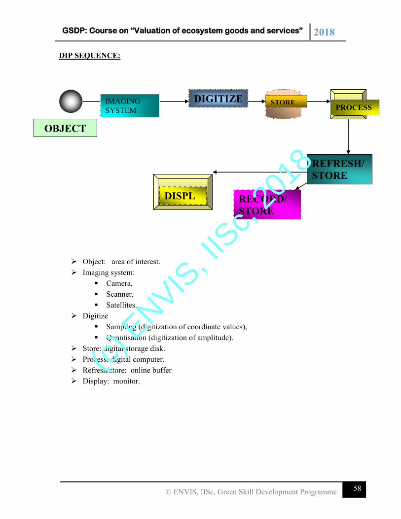
GSDP: Course on “Valuation of ecosystem goods and services” 2018
58 © ENVIS, IISc, Green Skill Development Programme
DIP SEQUENCE:
Object: area of interest.
Imaging system:
Camera,
Scanner,
Satellites.
Digitize
Sampling (digitization of coordinate values),
Quantisation (digitization of amplitude).
Store: digital storage disk.
Process: digital computer.
Refresh/store: online buffer
Display: monitor.
OBJECT
IMAGING
SYSTEM
DIGITIZE STORE PROCESS
REFRESH/
STORE
RECORD/
STORE
DISPL
AY
(c) E
NVIS, I
ISc,
2018
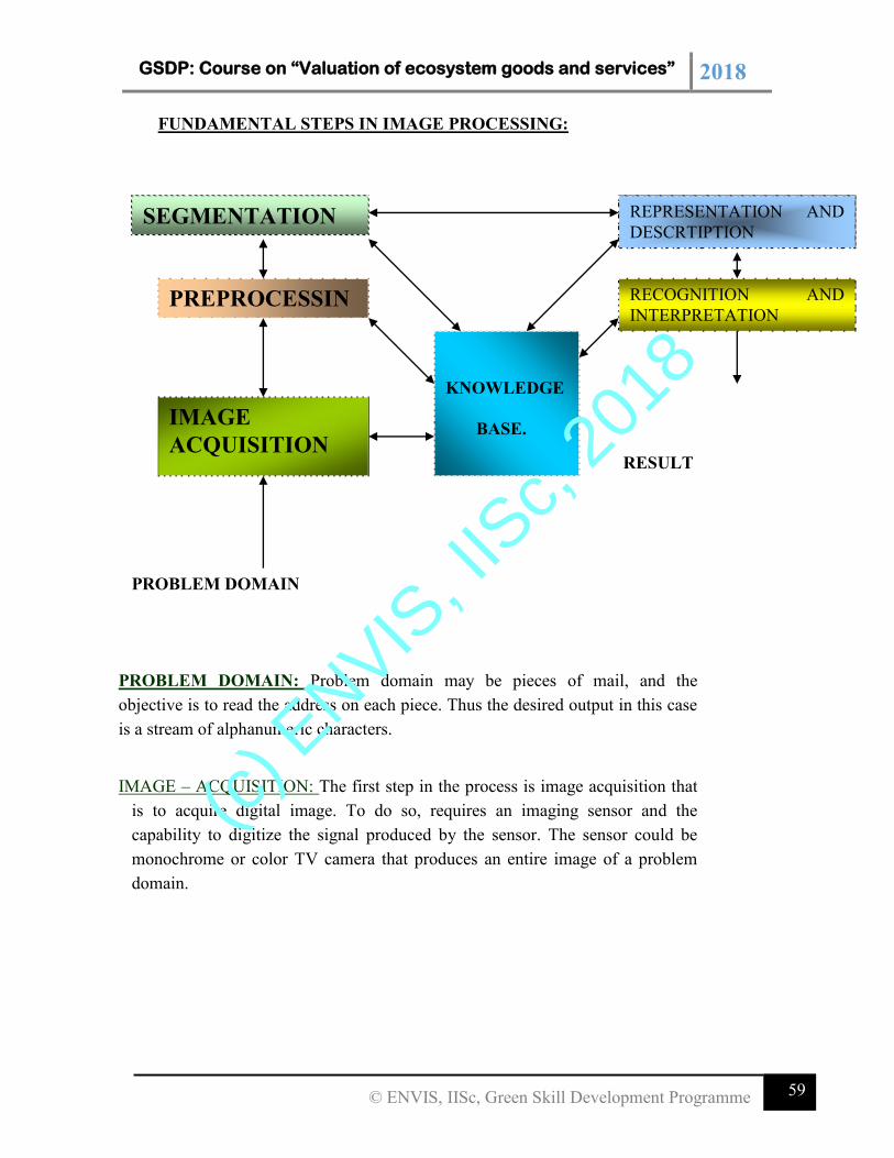
GSDP: Course on “Valuation of ecosystem goods and services” 2018
59 © ENVIS, IISc, Green Skill Development Programme
FUNDAMENTAL STEPS IN IMAGE PROCESSING:
RESULT
PROBLEM DOMAIN
PROBLEM DOMAIN: Problem domain may be pieces of mail, and the
objective is to read the address on each piece. Thus the desired output in this case
is a stream of alphanumeric characters.
IMAGE – ACQUISITION: The first step in the process is image acquisition that
is to acquire digital image. To do so, requires an imaging sensor and the
capability to digitize the signal produced by the sensor. The sensor could be
monochrome or color TV camera that produces an entire image of a problem
domain.
SEGMENTATION REPRESENTATION AND
DESCRTIPTION
PREPROCESSIN
G
RECOGNITION AND
INTERPRETATION
KNOWLEDGE
BASE. IMAGE
ACQUISITION
(c) E
NVIS, I
ISc,
2018
GSDP: Course on “Valuation of ecosystem goods and services” 2018
60 © ENVIS, IISc, Green Skill Development Programme
PREPROCESSING: The main objective of preprocessing is to improve the
image in ways that increase the chance for success of the other process. Ex:
Enhancing contrast, noise removal, and isolating regions.
SEGMENTATION: Segmentation is the process of partitioning an image
into its constituent parts.
REPRESENTATION AND DESCRIPTION: Representation is the only part of
solution for transforming raw data into a form suitable for subsequent computer
processing. Here the method should also be specified describing data so that
features of interests are highlighted.
Description is also called as feature selection which deals with extracting
features result in some quantitative information of interest or features that are
basic for differentiating one class of objects from another.
Recognition and interpretation: Recognition is a process that assigns the label to
an object based on the information provided by the descriptors. Interpretation
involves assigning meanings to an ensemble of recognised objects.
Knowledge base: Knowledge about the problem domain is coded into an image
processing system in the form of knowledge database. The order to guide the
operation of each processing module, the knowledge base also controls the
interaction between modules.
Digital data
Electronic imagery-A digital image is composed of many thousands of pixels. Each
pixels representing brightness of small portion of earth’s surface
Optical mechanical scanners-Physically move the mirror or lens to systematically
aim the view of earth’s surface. As the instrument scans the earth’s surface it
generates a electric current that varies in intensity as the land surface varies in
(c) E
NVIS, I
ISc,
2018
GSDP: Course on “Valuation of ecosystem goods and services” 2018
61 © ENVIS, IISc, Green Skill Development Programme
brightness. Each signal is subdivide into discrete units to create discrete values for
digital analysis
Charge coupled devices (CCDs)
Light sensitive material embedded in silicon chip
Sensitive components of CCD are manufactured as small 1µm in diameter
and sensitive to visible and near IR radiation
Detector collects photons that strikes a surface and accumulates a charge
proportional to the intensity of radiation
CCDs are compact and more efficient in detecting photons, effective even
when intensities are dim.
CCDs expose all pixels at the same instant than read these values as the next
image is acquired.
Low noise
CCD can be positioned in the focal plane of a sensor such that they view a thin
rectangular strip oriented at right angle to the flight path. The forward motion of
aircraft or satellite moves the field of view forward building up coverage.
Image Interpretation
Subject – Knowledge of subject of interpretation
Geographic Region – Knowledge of specific geographic region depicted on the
image.
Remote Sensing System – Interpreter must understand the formation of images
and function of sensor in the portrayal of landscape.
Classification- Assignment of object, area, features based on their appearance on
imagery.
Detection – Determination of presence or absence of a feature
Recognition – Higher level of knowledge about a feature
Identification – Identity of a given feature can be specified with enough
confidence.
(c) E
NVIS, I
ISc,
2018
GSDP: Course on “Valuation of ecosystem goods and services” 2018
62 © ENVIS, IISc, Green Skill Development Programme
Enumeration- Task of listing or counting discrete items present on an image.
Measurement -
Measurement of distance and height
Extension of volumes and areas as well.
Delineation –
Interpreter must delineate or outline regions as observed on remotely sensed
data.
Interpreter must be able to separate distinct areal units characterized by
specific tones and textures.
Identify edges or boundaries between separate areas.
Elements of Image interpretation
Image tone- denotes lightness or darkness of a region within an image
For black and white images – tones may be characterized by light, medium gray,
dark gray.
For colour images- tones simply refers to colours. Image tone refers ultimately to the
brightness of an area of the ground.
Hue refers to the colour on the image as defined in the intensity-hue –saturation
(IHS).
Tonal variations are an important interpretation element in an image
interpretation.
The tonal expression of object on the image is directly related to the amount of
light reflected from its surface.
Different types of rock, soil or vegetation most likely have different tones.
Image texture- Apparent roughness or smoothness of an image.
Usually image texture is caused by pattern of highlighted and shadowed area
created when an irregular surface is illuminated with an oblique angle.
Image texture depends on the surface and the angle of illumination.
Shadow
Provides an important clue
(c) E
NVIS, I
ISc,
2018
GSDP: Course on “Valuation of ecosystem goods and services” 2018
63 © ENVIS, IISc, Green Skill Development Programme
Features illuminated at an angle cast a shadow that reveal characteristic of its
shape and size.
Military photo interpreters have developed techniques to use shadows to
distinguish subtle difference that might not show otherwise.
Useful in identification of man-made landscape
Pattern
Arrangement of individual objects into distinctive recurring form that
facilitate the recognition.
Pattern can be described by terms such as concentric, radial, checkerboard,
etc.
Some land uses however have specific and characteristic pattern when
observed from on aerospace data.
Examples include the hydrological system rivers with its branches and
patterns related to erosion.
Association
When identification of a specific class of equipment implies that other more
important items are likely to be found nearby.
An example of association is an interpretation of a thermal power plant based
on the combined recognition of high chimneys, large buildings, cooling
towers, coal heaps etc.
Shape
Obvious clues of their identity
Individual structures have characteristic shapes.
Height differences are important to distinguish between different vegetation
types and also in geomorphological mapping. The shape of objects often helps
to determine the character of the object (build up, roads and railways
agricultural fields etc.).
Size
Relative size of the other object in relation to the other objects on the image
provides the interpreter with the notion of its scale and resolution.
Accurate measurement can be valuable as interpretation aid.
The width of road can be estimated by comparing it to the size of the cars,
which is generally known. Subsequently this width determine the road type,
e.g. primary road, secondary road etc.
(c) E
NVIS, I
ISc,
2018
GSDP: Course on “Valuation of ecosystem goods and services” 2018
64 © ENVIS, IISc, Green Skill Development Programme
Site
Refers to topological positions
Sewage treatment facility is positioned near low topological sites near the
steams or rivers to collect the waste water flowing from high location.
A typical example of this interpolation element is that back swamps can be
found in a flood plain but not in the centre of city area.
The possible forms of digital image manipulation:
1. Image restoration and rectification
2. Image enhancement
3. Image classification
4. Data merging & GIS integration
5. Biophysical modeling
Image rectification and restoration
These operations aim to correct distorted or degraded image data to create a
more faithful representation of the original scene.
- Corrections for geometric distortions,
- Calibrate the data radio metrically
- To eliminate noise present in the data
Remotely sensed images of the environment are typically taken at a great distance from
the earth’s surface. As a result, there is a substantial atmospheric path that
electromagnetic energy must pass through before it reaches the sensor. Depending upon
the wavelengths involved and atmospheric conditions (such as particulate matter,
moisture content and turbulence), the incoming energy may be substantially modified.
The sensor itself may then modify the character of that data since it may combine a
variety of mechanical, optical and electrical components that serve to modify or mask the
measured radiant energy. In addition, during the time the image is being scanned, the
satellite is following a path that is subject to minor variations at the same time that the
earth is moving underneath. The geometry of the image is thus in constant flux. Finally,
the signal needs to be tele-metered back to the earth, and subsequently received and
processed to yield the final data we receive. Consequently, a variety of systematic and
apparently random disturbances can combine to degrade the quality of the image we
finally receive. Image restoration seeks to remove these degradation effects.
(c) E
NVIS, I
ISc,
2018
GSDP: Course on “Valuation of ecosystem goods and services” 2018
65 © ENVIS, IISc, Green Skill Development Programme
Broadly, the image restoration can be broken down into the two sub-areas of radiometric
restoration and geometric restoration.
Geometric Restoration: For mapping purposes, it is essential that any form of remotely
sensed imagery be accurately registered to the purposed map base. With satellite imagery,
the very high altitude of the sensing platform results in minimal image displacements due
to relief. As a result, registration can usually be achieved through the use of a systematic
rubber sheet transformation process that gently warps an image (through the use of
polynomial equations) based on the known positions of a set of widely dispersed control
points.
With aerial photographs, however, the process is more complex. Not only are there
systematic distortions related to tilt and varying altitude, but variable topographic relief
leads to very irregular distortions (differential parallax) that cannot be removed through a
rubber sheet transformation procedure. In these instances, it is necessary to use
photogrammetric rectification to remove these distortions and provide accurate map
measurements. Failing this, the central portions of high altitude photographs can be
resampled with some success. Doing so also requires a thorough understanding of
reference systems and their associated parameters such as datums and projections.
The sources of geometric distortions:
- Variations in the altitude,
- Velocity of the sensor platform
- Earth curvature
- Atmospheric refraction
It is implemented as a two-step procedure:
- Systematic or predictable distortions
- Random or unpredictable distortions
Systematic distortions are well understood and easily corrected by applying formulas
derived by modeling the sources of distortions mathematically. Random distortions are
residual unknown systematic distortions are corrected by analyzing well-distributed
ground control points occurring in an image.
(c) E
NVIS, I
ISc,
2018
GSDP: Course on “Valuation of ecosystem goods and services” 2018
66 © ENVIS, IISc, Green Skill Development Programme
Radiometric Restoration: Radiometric restoration refers to the removal or
diminishment of distortions in the degree of electromagnetic energy registered by each
detector. A variety of agents can cause distortion in the values recorded for image cells.
Some of the most common distortions for which correction procedures exist include:
Uniformly elevated values, due to atmospheric haze, which preferentially scatters
short wavelength bands (particularly the blue wavelength);
Striping, due to detectors going out of calibration;
Random noise, due to unpredictable and unsystematic performance of the sensor
or transmission of the data; and
Scan line drop out, due to signal loss from specific detectors.
It is also appropriate to include here procedures that are used to convert the raw, uniless
relative reflectance values (known as digital numbers, or DN) of the original bands into
true measures of reflective power (radiance).
Radiance measured by any given system over a given object is influenced by
such factors as:
Changes in scene illumination,
Atmospheric conditions,
Viewing geometry, and
Instrument response characteristics
Sun – elevation correction and Earth-sun distance correction
The earth-sun distance correction is applied to normalize for the seasonal
changes in the distance between the earth and the sun.
The combined effect of solar-zenith angle and earth-sun distance on the
irradiance incident on the earth’s surface can be expressed as,
E = (E0 * Cos q0) / (d^2) where,
E = normalized solar irradiance
E0 = solar irradiance at mean earth-sun distance
q0 = sun’s angle from the zenith
d=earth-sun distance in AU [ASTRONOMICAL UNITS]
(c) E
NVIS, I
ISc,
2018
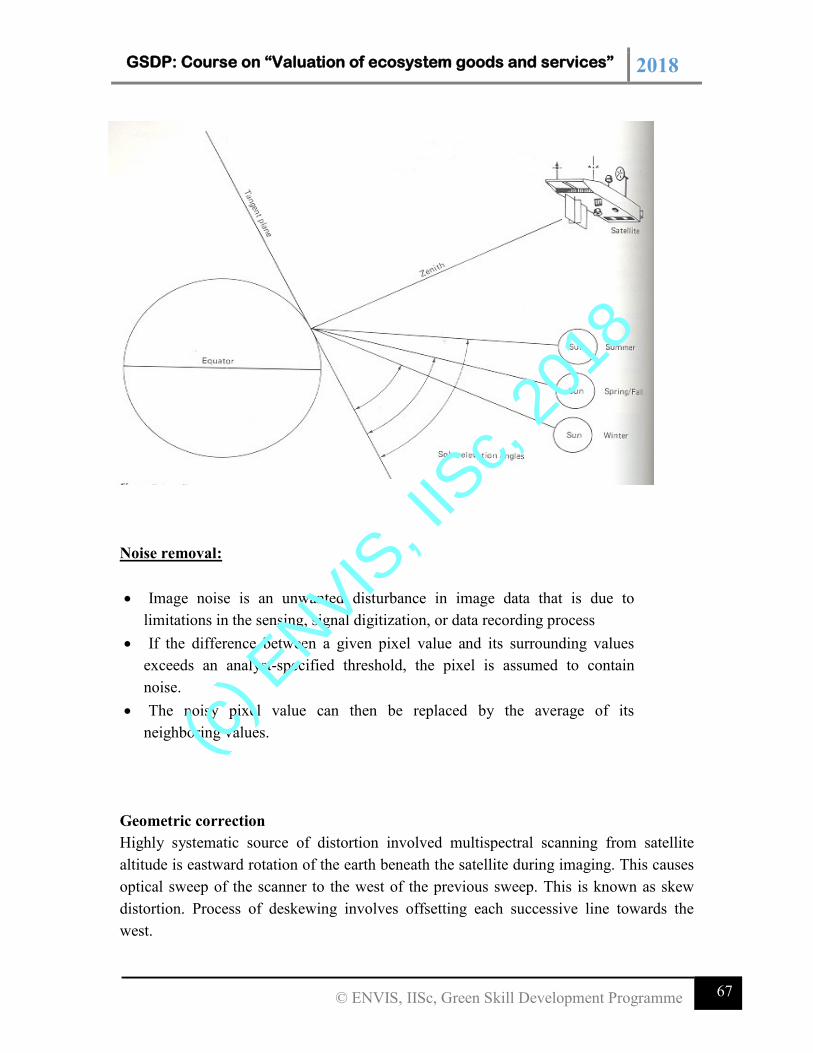
GSDP: Course on “Valuation of ecosystem goods and services” 2018
67 © ENVIS, IISc, Green Skill Development Programme
Noise removal:
Image noise is an unwanted disturbance in image data that is due to
limitations in the sensing, signal digitization, or data recording process
If the difference between a given pixel value and its surrounding values
exceeds an analyst-specified threshold, the pixel is assumed to contain
noise.
The noisy pixel value can then be replaced by the average of its
neighboring values.
Geometric correction
Highly systematic source of distortion involved multispectral scanning from satellite
altitude is eastward rotation of the earth beneath the satellite during imaging. This causes
optical sweep of the scanner to the west of the previous sweep. This is known as skew
distortion. Process of deskewing involves offsetting each successive line towards the
west.
(c) E
NVIS, I
ISc,
2018
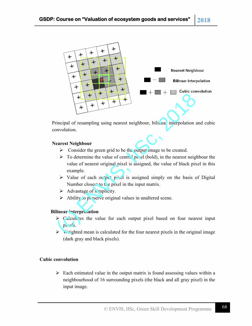
GSDP: Course on “Valuation of ecosystem goods and services” 2018
68 © ENVIS, IISc, Green Skill Development Programme
Principal of resampling using nearest neighbour, bilinear interpolation and cubic
convolution.
Nearest Neighbour
Consider the green grid to be the output image to be created.
To determine the value of central pixel (bold), in the nearest neighbour the
value of nearest original pixel is assigned, the value of black pixel in this
example.
Value of each output pixel is assigned simply on the basis of Digital
Number closest to the pixel in the input matrix.
Advantage of simplicity.
Ability to preserve original values in unaltered scene.
Bilinear interpretation
Calculates the value for each output pixel based on four nearest input
pixels.
Weighted mean is calculated for the four nearest pixels in the original image
(dark gray and black pixels).
Cubic convolution
Each estimated value in the output matrix is found assessing values within a
neighbourhood of 16 surrounding pixels (the black and all gray pixel) in the
input image.
(c) E
NVIS, I
ISc,
2018
GSDP: Course on “Valuation of ecosystem goods and services” 2018
69 © ENVIS, IISc, Green Skill Development Programme
Radiometric corrections-
Radiance measured by any given system over an object is influenced by-
Scene illumination
Atmospheric conditions
Viewing geometry
Instrument response
Radiometric corrections can be divided into relatively simple cosmetic
rectification, as well as atmospheric corrections.
Atmospheric corrections constitute an important step on the preprocessing
of remotely sensed data. Their effect is to rescale the atmospheric raw
radiance data.
Image data acquired under different solar illumination angles are normalized
by calculating pixel brightness values assuming that sun was at zenith
during each day of sensing.
The correction is applied by dividing each pixel in a scene by sine of solar
elevation angle for particular time and location of imaging.
Noise Removal
Random noise or spike noise
Image noise is the unwanted disturbance in image data.
Noise removal is done before any subsequent enhancement or classification
of image data.
The periodic line dropouts and striping are forms of random noise that may
be recognized and restored by simple means. Random noise on the other
hand, requires a more sophisticated restoration process such as digital
filtering.
Random noise or temporary noise may be due to errors during transmission
of data or temporary disturbance.
Individual pixels acquire DN – values that are much higher and lower than the
surrounding pixels. In image they produce a bright and dark spot that interferes with the
information extraction procedures.
Spike noise can be detected by mutually comparing neighbouring pixel
values. If neighbouring pixel values differ by more than threshold margin, it
(c) E
NVIS, I
ISc,
2018
GSDP: Course on “Valuation of ecosystem goods and services” 2018
70 © ENVIS, IISc, Green Skill Development Programme
is designated as spike noise and the DN is replaced by an interpolated DN
value.
De-striping
One method is to compile a set of histograms for the image –one for each
detector involved in a given band.
These histograms are then compared in terms of their mean and median
values to identify problem detector.
A grey scale adjustment factor is applied to adjust the histograms for
problem lines and others are not altered.
Line striping occurs due to non identical detectors response.
Although the detectors for all satellite sensors are carefully calibrated and
matched before launch of the satellite, with time response of some detectors
may drift to higher or lower levels.
Every scan lines are brighter or darker than the other lines. It is important to
understand that valid datas are present in the defective lines, but that must
be corrected to match the overall scene.
Periodic Line dropouts
A number of adjacent pixels along a line or an entire line may contain defective
Digital Number
This problem is addressed by replacing defective Digital Number with the
average of values for the pixels occurring in the line below and above.
Digital Number from the preceding line can simply be inserted in the defective
pixel.
Image enhancement: Image enhancement is concerned with the
modification of images to make them more suited to the capabilities of human
vision. Regardless of the extent of digital intervention, visual analysis invariably
plays a very strong role in all aspects of remote sensing. While the range of
image enhancement techniques is broad, the following fundamental issues form
the backbone of this area These procedures applied to image data in order to
more effectively display or record the data for subsequent visual interpretation.
Contrast manipulation
(c) E
NVIS, I
ISc,
2018
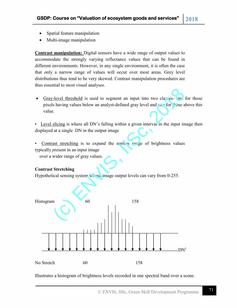
GSDP: Course on “Valuation of ecosystem goods and services” 2018
71 © ENVIS, IISc, Green Skill Development Programme
Spatial feature manipulation
Multi-image manipulation
Contrast manipulation: Digital sensors have a wide range of output values to
accommodate the strongly varying reflectance values that can be found in
different environments. However, in any single environment, it is often the case
that only a narrow range of values will occur over most areas. Grey level
distributions thus tend to be very skewed. Contrast manipulation procedures are
thus essential to most visual analyses.
Gray-level threshold is used to segment an input into two classes- one for those
pixels having values below an analyst-defined gray level and one for those above this
value.
• Level slicing is where all DN’s falling within a given interval in the input image then
displayed at a single DN in the output image
• Contrast stretching is to expand the narrow range of brightness values
typically present in an input image
over a wider range of gray values.
Contrast Stretching
Hypothetical sensing system whose image output levels can vary from 0-255.
Histogram 60 158
DN1
No Stretch 60 158
Illustrates a histogram of brightness levels recorded in one spectral band over a scene.
(c) E
NVIS, I
ISc,
2018
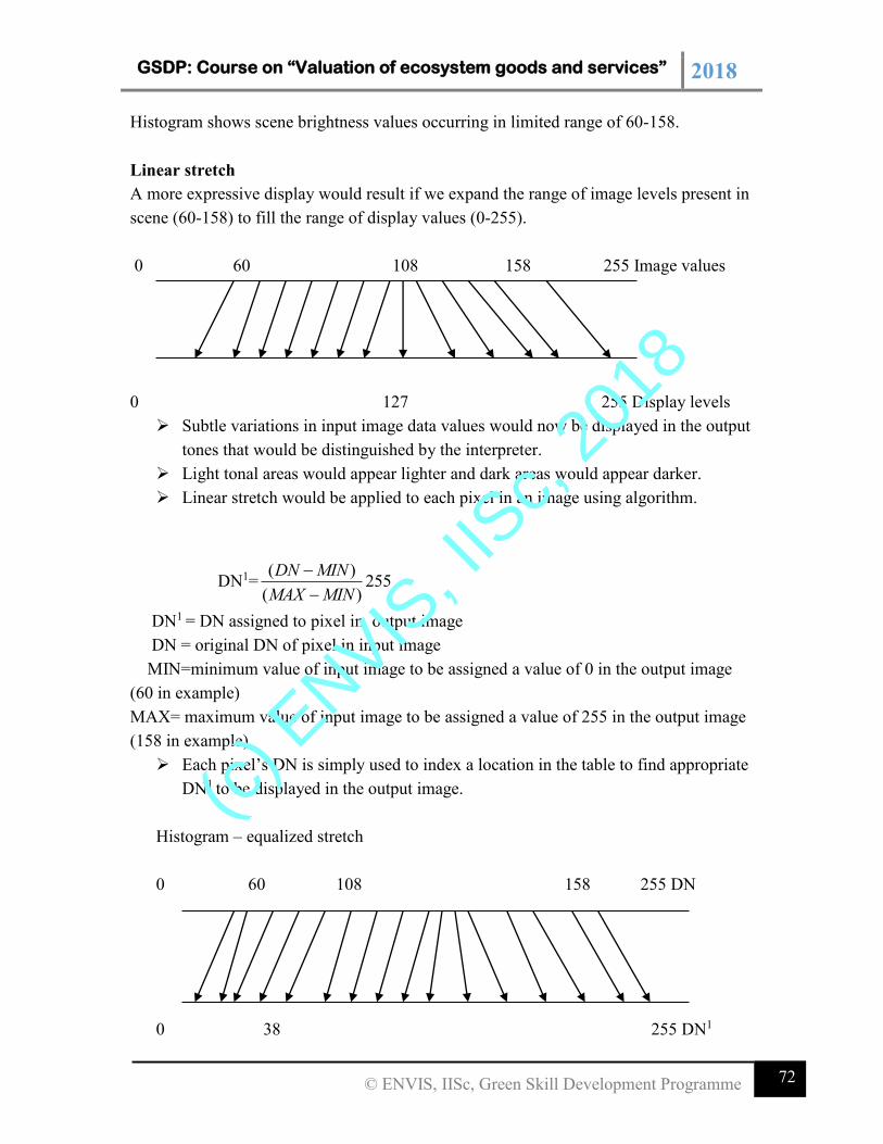
GSDP: Course on “Valuation of ecosystem goods and services” 2018
72 © ENVIS, IISc, Green Skill Development Programme
Histogram shows scene brightness values occurring in limited range of 60-158.
Linear stretch
A more expressive display would result if we expand the range of image levels present in
scene (60-158) to fill the range of display values (0-255).
0 60 108 158 255 Image values
0 127 255 Display levels
Subtle variations in input image data values would now be displayed in the output
tones that would be distinguished by the interpreter.
Light tonal areas would appear lighter and dark areas would appear darker.
Linear stretch would be applied to each pixel in an image using algorithm.
DN1=( )
255( )
DN MIN
MAX MIN
DN1 = DN assigned to pixel in output image
DN = original DN of pixel in input image
MIN=minimum value of input image to be assigned a value of 0 in the output image
(60 in example)
MAX= maximum value of input image to be assigned a value of 255 in the output image
(158 in example)
Each pixel’s DN is simply used to index a location in the table to find appropriate
DN1 to be displayed in the output image.
Histogram – equalized stretch
0 60 108 158 255 DN
0 38 255 DN1
(c) E
NVIS, I
ISc,
2018
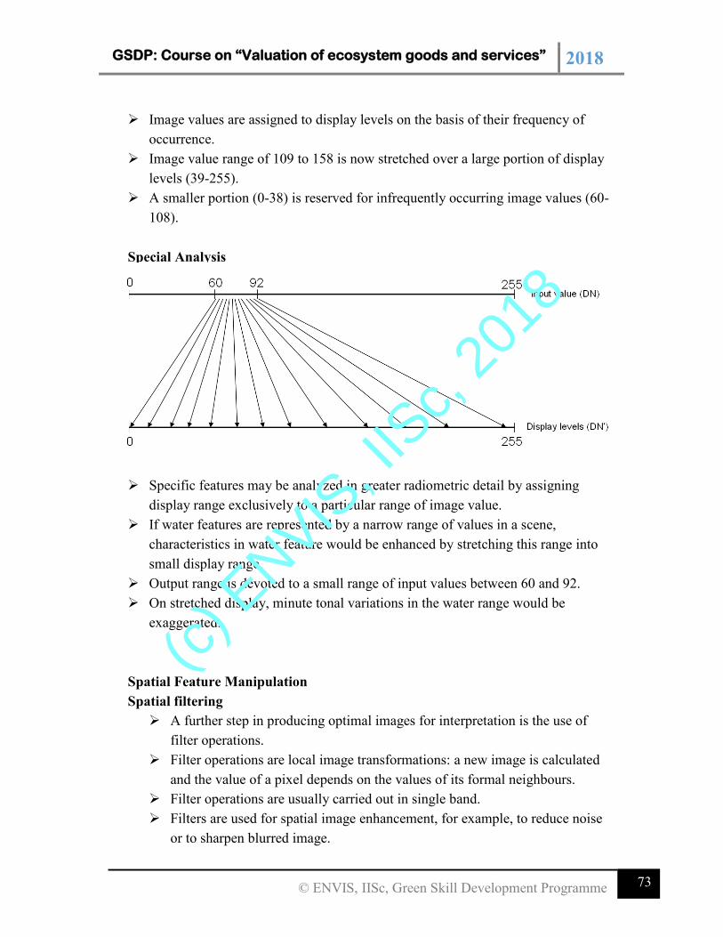
GSDP: Course on “Valuation of ecosystem goods and services” 2018
73 © ENVIS, IISc, Green Skill Development Programme
Image values are assigned to display levels on the basis of their frequency of
occurrence.
Image value range of 109 to 158 is now stretched over a large portion of display
levels (39-255).
A smaller portion (0-38) is reserved for infrequently occurring image values (60-
108).
Special Analysis
Specific features may be analyzed in greater radiometric detail by assigning
display range exclusively to a particular range of image value.
If water features are represented by a narrow range of values in a scene,
characteristics in water feature would be enhanced by stretching this range into
small display range.
Output range is devoted to a small range of input values between 60 and 92.
On stretched display, minute tonal variations in the water range would be
exaggerated.
Spatial Feature Manipulation
Spatial filtering
A further step in producing optimal images for interpretation is the use of
filter operations.
Filter operations are local image transformations: a new image is calculated
and the value of a pixel depends on the values of its formal neighbours.
Filter operations are usually carried out in single band.
Filters are used for spatial image enhancement, for example, to reduce noise
or to sharpen blurred image.
(c) E
NVIS, I
ISc,
2018
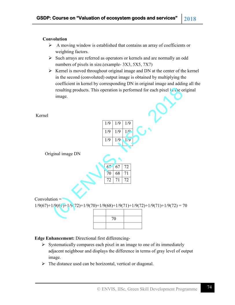
GSDP: Course on “Valuation of ecosystem goods and services” 2018
74 © ENVIS, IISc, Green Skill Development Programme
Convolution
A moving window is established that contains an array of coefficients or
weighting factors.
Such arrays are referred as operators or kernels and are normally an odd
numbers of pixels in size.(example- 3X3, 5X5, 7X7)
Kernel is moved throughout original image and DN at the center of the kernel
in the second (convoluted) output image is obtained by multiplying the
coefficient in kernel by corresponding DN in original image and adding all the
resulting products. This operation is performed for each pixel in the original
image.
Kernel
Original image DN
67 67 72
70 68 71
72 71 72
Convolution =
1/9(67)+1/9(67)+1/9(72)+1/9(70)+1/9(68)+1/9(71)+1/9(72)+1/9(71)+1/9(72) = 70
70
Edge Enhancement: Directional first differencing-
Systematically compares each pixel in an image to one of its immediately
adjacent neighbour and displays the difference in terms of gray level of output
image.
The distance used can be horizontal, vertical or diagonal.
1/9 1/9 1/9
1/9 1/9 1/9
1/9 1/9 1/9
(c) E
NVIS, I
ISc,
2018
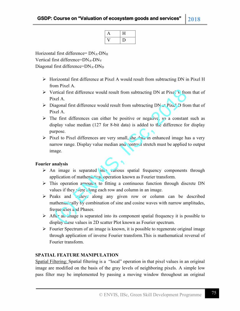
GSDP: Course on “Valuation of ecosystem goods and services” 2018
75 © ENVIS, IISc, Green Skill Development Programme
A H
V D
Horizontal first difference= DNA-DNH
Vertical first difference=DNA-DNV
Diagonal first difference=DNA-DND
Horizontal first difference at Pixel A would result from subtracting DN in Pixel H
from Pixel A.
Vertical first difference would result from subtracting DN at Pixel V from that of
Pixel A.
Diagonal first difference would result from subtracting DN at Pixel D from that of
Pixel A.
The first differences can either be positive or negative, so a constant such as
display value median (127 for 8-bit data) is added to the difference for display
purpose.
Pixel to Pixel differences are very small, the data in enhanced image has a very
narrow range. Display value median and contrast stretch must be applied to output
image.
Fourier analysis
An image is separated into various spatial frequency components through
application of mathematical operation known as Fourier transform.
This operation amounts to fitting a continuous function through discrete DN
values if they were along each row and column in an image.
Peaks and valleys along any given row or column can be described
mathematically by combination of sine and cosine waves with narrow amplitudes,
frequencies and Phases.
After an image is separated into its component spatial frequency it is possible to
display these values in 2D scatter Plot known as Fourier spectrum.
Fourier Spectrum of an image is known, it is possible to regenerate original image
through application of inverse Fourier transform.This is mathematical reversal of
Fourier transform.
SPATIAL FEATURE MANIPULATION
Spatial Filtering: Spatial filtering is a “local” operation in that pixel values in an original
image are modified on the basis of the gray levels of neighboring pixels. A simple low
pass filter may be implemented by passing a moving window throughout an original
(c) E
NVIS, I
ISc,
2018
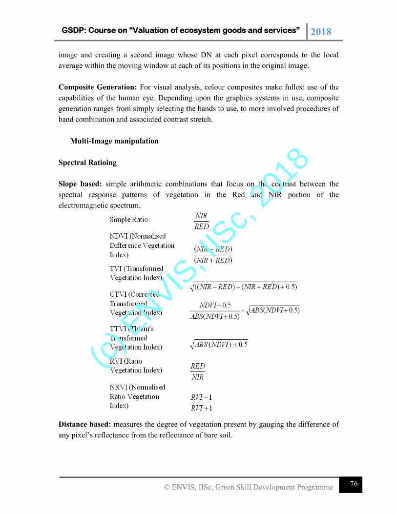
GSDP: Course on “Valuation of ecosystem goods and services” 2018
76 © ENVIS, IISc, Green Skill Development Programme
image and creating a second image whose DN at each pixel corresponds to the local
average within the moving window at each of its positions in the original image.
Composite Generation: For visual analysis, colour composites make fullest use of the
capabilities of the human eye. Depending upon the graphics systems in use, composite
generation ranges from simply selecting the bands to use, to more involved procedures of
band combination and associated contrast stretch.
Multi-Image manipulation
Spectral Ratioing
Slope based: simple arithmetic combinations that focus on the contrast between the
spectral response patterns of vegetation in the Red and NIR portion of the
electromagnetic spectrum.
Distance based: measures the degree of vegetation present by gauging the difference of
any pixel’s reflectance from the reflectance of bare soil.
(c) E
NVIS, I
ISc,
2018
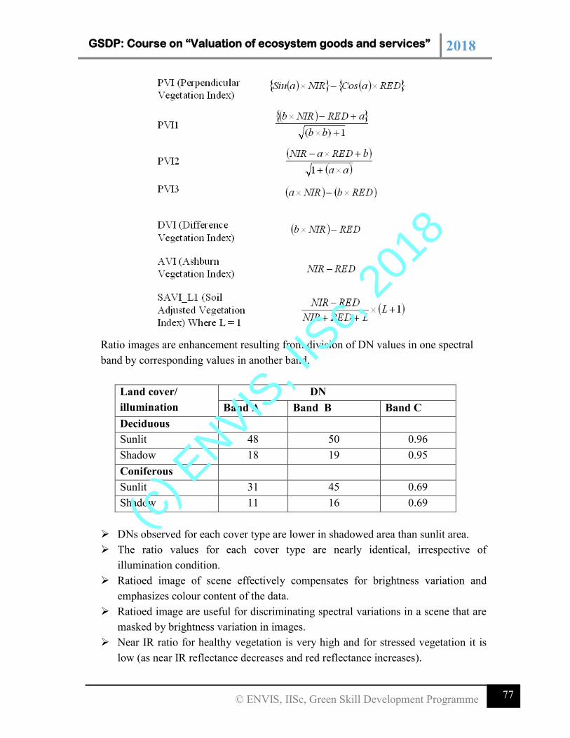
GSDP: Course on “Valuation of ecosystem goods and services” 2018
77 © ENVIS, IISc, Green Skill Development Programme
Ratio images are enhancement resulting from division of DN values in one spectral
band by corresponding values in another band.
Land cover/
illumination
DN
Band A Band B Band C
Deciduous
Sunlit 48 50 0.96
Shadow 18 19 0.95
Coniferous
Sunlit 31 45 0.69
Shadow 11 16 0.69
DNs observed for each cover type are lower in shadowed area than sunlit area.
The ratio values for each cover type are nearly identical, irrespective of
illumination condition.
Ratioed image of scene effectively compensates for brightness variation and
emphasizes colour content of the data.
Ratioed image are useful for discriminating spectral variations in a scene that are
masked by brightness variation in images.
Near IR ratio for healthy vegetation is very high and for stressed vegetation it is
low (as near IR reflectance decreases and red reflectance increases).
(c) E
NVIS, I
ISc,
2018
GSDP: Course on “Valuation of ecosystem goods and services” 2018
78 © ENVIS, IISc, Green Skill Development Programme
Thus, near IR to red (or red to near IR) ratioed image might be very useful for
differentiating between area of stressed and non stressed vegetation.
The form and number of ratio combinations available to image analyst varies
depending on the source of digital data.
The number of possible ratios that can be developed from n bands of data is
n(n-1). Thus, Landsat MSS data, 4(4-1), 12 different ratio combinations are
possible (six original and six reciprocal).
The ratio TM3/TM4 is depicted so that the features such as water and roads which
reflects highly in the red band (TM3) and little in IR band (TM4) are shown in
lighter tones.
Features such as vegetation appears in darker tones because of its low reflectance
in red band (TM3) and high reflectance in near IR (TM4).
Ratio TM5/TM2, vegetation appears in light tones because of its high reflectance
in mid IR band and low reflectance in green band (TM2).
Ratio TM3/TM7, roads and other cultural features appear in lighter tones in this
image due to high reflectance in red band (TM3) and low reflectance in mid-IR
band (TM7).
Differences in water turbidity are readily observable in ratio image.
Ratio images can be used to generate false colour composites by combining three
monochromatic ratio datasets.
Such composites have two fold advantages of combining data from more than two
bands and presenting it in colour which facilitates interpretation of subtle spectral
reflectance differences.
20 colour combinations are possible when 6 original ratios of landsat MSS data
are displayed 3 at a time.
15 original ratio of non thermal ratio of non thermal TM data result in 455
different possible combinations.
Caution should be taken generating and interpreting ratio images.
Such images are intensity blind. (c) E
NVIS, I
ISc,
2018
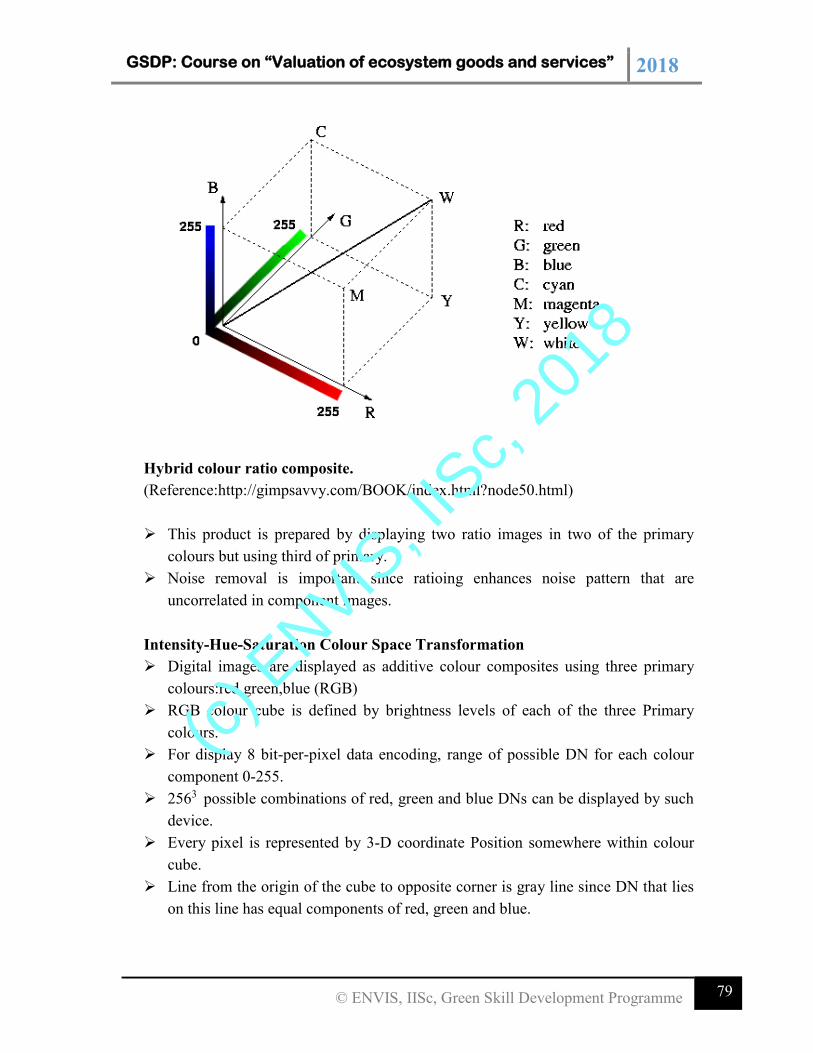
GSDP: Course on “Valuation of ecosystem goods and services” 2018
79 © ENVIS, IISc, Green Skill Development Programme
Hybrid colour ratio composite.
(Reference:http://gimpsavvy.com/BOOK/index.html?node50.html)
This product is prepared by displaying two ratio images in two of the primary
colours but using third of primary.
Noise removal is important since ratioing enhances noise pattern that are
uncorrelated in component images.
Intensity-Hue-Saturation Colour Space Transformation
Digital images are displayed as additive colour composites using three primary
colours:red,green,blue (RGB)
RGB colour cube is defined by brightness levels of each of the three Primary
colours.
For display 8 bit-per-pixel data encoding, range of possible DN for each colour
component 0-255.
2563 possible combinations of red, green and blue DNs can be displayed by such
device.
Every pixel is represented by 3-D coordinate Position somewhere within colour
cube.
Line from the origin of the cube to opposite corner is gray line since DN that lies
on this line has equal components of red, green and blue.
(c) E
NVIS, I
ISc,
2018
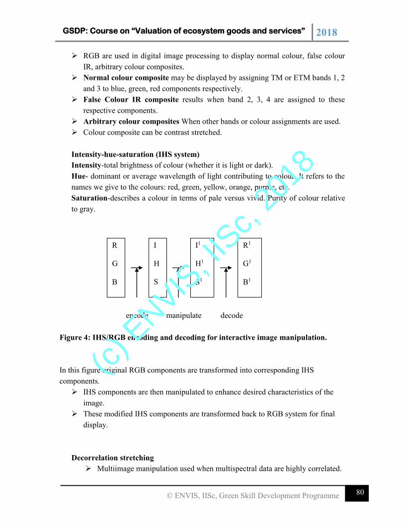
GSDP: Course on “Valuation of ecosystem goods and services” 2018
80 © ENVIS, IISc, Green Skill Development Programme
RGB are used in digital image processing to display normal colour, false colour
IR, arbitrary colour composites.
Normal colour composite may be displayed by assigning TM or ETM bands 1, 2
and 3 to blue, green, red components respectively.
False Colour IR composite results when band 2, 3, 4 are assigned to these
respective components.
Arbitrary colour composites When other bands or colour assignments are used.
Colour composite can be contrast stretched.
Intensity-hue-saturation (IHS system)
Intensity-total brightness of colour (whether it is light or dark).
Hue- dominant or average wavelength of light contributing to colour. It refers to the
names we give to the colours: red, green, yellow, orange, purple, etc.
Saturation-describes a colour in terms of pale versus vivid. Purity of colour relative
to gray.
encode manipulate decode
Figure 4: IHS/RGB encoding and decoding for interactive image manipulation.
In this figure original RGB components are transformed into corresponding IHS
components.
IHS components are then manipulated to enhance desired characteristics of the
image.
These modified IHS components are transformed back to RGB system for final
display.
Decorrelation stretching
Multiimage manipulation used when multispectral data are highly correlated.
R
G
B
I
H
S
I1
H1
S1
R1
G1
B1
(c) E
NVIS, I
ISc,
2018
GSDP: Course on “Valuation of ecosystem goods and services” 2018
81 © ENVIS, IISc, Green Skill Development Programme
Traditional contrast stretching of highly correlated data as R, G, and B
displays normally only expands the range of intensities.
Decorrelation stretching involves exaggeration of least correlated information
in an image primarily in terms of saturation with minimal change in image
intensity and hue.
IHS transformation, decorrelation stretching is applied in a transformed
image space, the results are transformed back to RGB system for final
display.
CLASSIFICATION
The term pattern refers to the set of radiance measurements obtained in the
various wavelength bands for each pixel.
Spectral pattern recognition refers to classification procedures that
utilize this pixel-by-pixel spectral information as the basis for automated
land cover classification.
Spatial Pattern recognition-Categorization of image pixels on the basis
of their spatial relationship with the pixel surrounding them. Spatial
classifier considers aspect such as – Image texture, pixel proximity,
feature size, shape directionality, repetition and context.
Temporal Pattern recognition-uses time as an aid in feature
identification. Distinct spectral and spatial changes during season can
permit discrimination on multidate imagery that would be impossible
given any single date.
Supervised Classification
Supervised classification - In this classification, the image analyst
“supervises” the pixel categorization process by specifying, to the computer
algorithm, numerical descriptors of the various land cover types present in a
scene.
One of the main steps in image classification is the partitioning of feature
space.
Supervised classification requires the operator to be familiar with the area of
interest.
The operator needs to know where to find the classes of interest in the area
covered in the image.
(c) E
NVIS, I
ISc,
2018
GSDP: Course on “Valuation of ecosystem goods and services” 2018
82 © ENVIS, IISc, Green Skill Development Programme
Three basic steps are involved:
1. Training stage - the analyst identifies representative training areas and
develops a numerical description of the spectral attributes of each land cover
type of interest in the scene.
2. Classification stage - each pixel in the image data set is categorized into the
land cover class it most closely resembles. The category label assigned to each
pixel in this process is then recorded in the corresponding cell of an interpreted
data set (an “output” image).
3. Output stage – After the entire data set has been categorized, the results are
presented in the output stage. Three typical forms of output products are
thematic maps, tables of full scene or sub scène area statistics for the various
land cover classes, and digital data files amenable to inclusion in a GIS.
THE CLASSIFICATION STAGE
Minimum-Distance-to-Means Classifier
Parallelepiped Classifier
Gaussian Maximum Likelihood Classifier
Each pixel in the image data set is categorized into class it closely
resembles. If pixel is insufficiently similar to any training data set it is
labeled as ‘unknown’.
Category label assigned to each pixel in this process is recorded in
corresponding cell of an interpreted data (output image).
After entire dataset has been categorized the results are presented in
output stage.
(c) E
NVIS, I
ISc,
2018
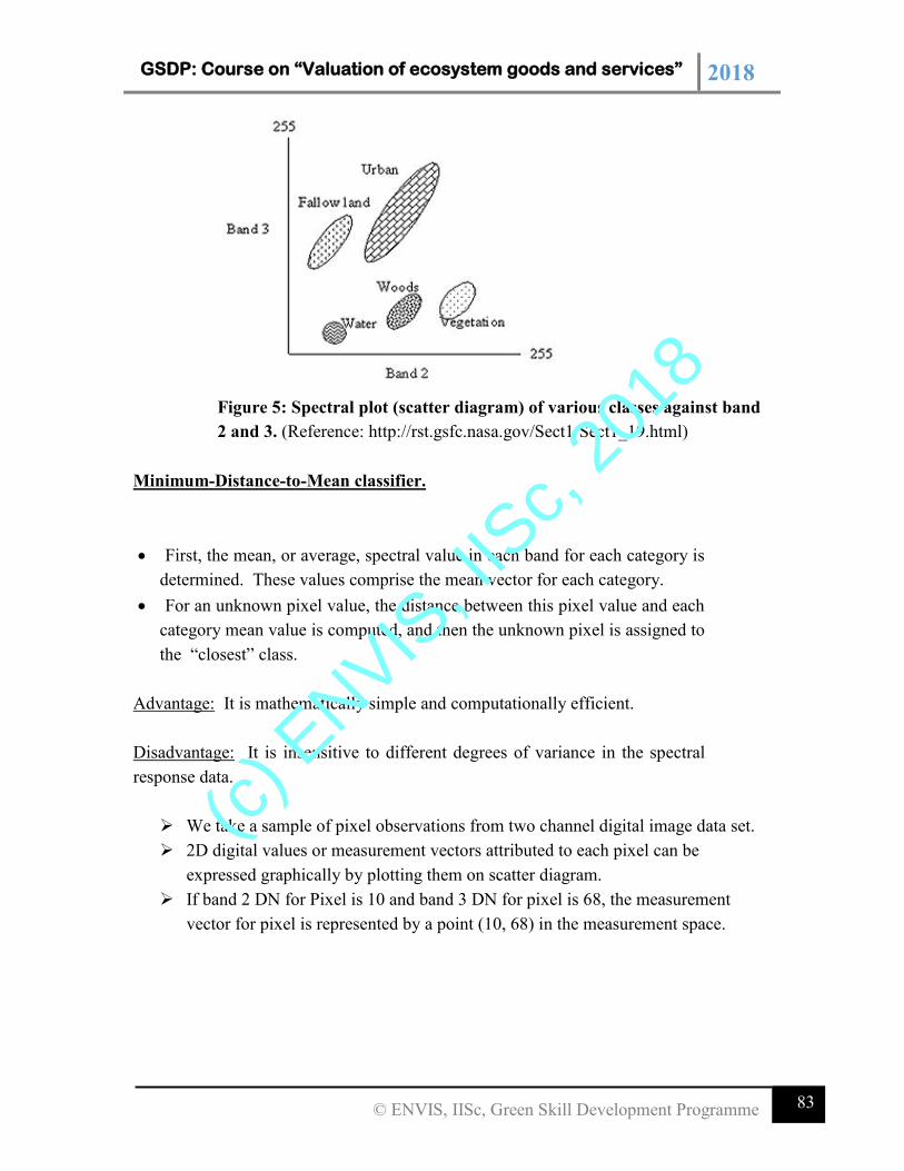
GSDP: Course on “Valuation of ecosystem goods and services” 2018
83 © ENVIS, IISc, Green Skill Development Programme
Figure 5: Spectral plot (scatter diagram) of various classes against band
2 and 3. (Reference: http://rst.gsfc.nasa.gov/Sect1/Sect1_19.html)
Minimum-Distance-to-Mean classifier.
First, the mean, or average, spectral value in each band for each category is
determined. These values comprise the mean vector for each category.
For an unknown pixel value, the distance between this pixel value and each
category mean value is computed, and then the unknown pixel is assigned to
the “closest” class.
Advantage: It is mathematically simple and computationally efficient.
Disadvantage: It is insensitive to different degrees of variance in the spectral
response data.
We take a sample of pixel observations from two channel digital image data set.
2D digital values or measurement vectors attributed to each pixel can be
expressed graphically by plotting them on scatter diagram.
If band 2 DN for Pixel is 10 and band 3 DN for pixel is 68, the measurement
vector for pixel is represented by a point (10, 68) in the measurement space.
(c) E
NVIS, I
ISc,
2018
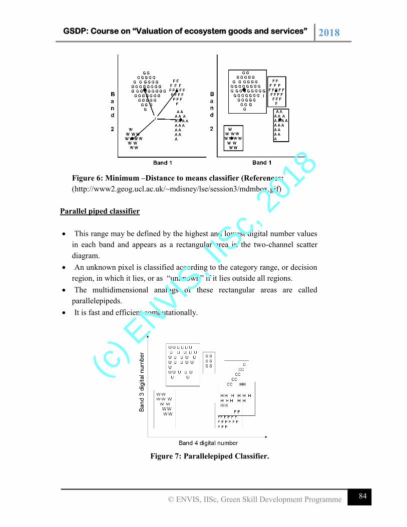
GSDP: Course on “Valuation of ecosystem goods and services” 2018
84 © ENVIS, IISc, Green Skill Development Programme
Figure 6: Minimum –Distance to means classifier (References:
(http://www2.geog.ucl.ac.uk/~mdisney/lse/session3/mdmbox.gif)
Parallel piped classifier
This range may be defined by the highest and lowest digital number values
in each band and appears as a rectangular area in the two-channel scatter
diagram.
An unknown pixel is classified according to the category range, or decision
region, in which it lies, or as “unknown” if it lies outside all regions.
The multidimensional analogs of these rectangular areas are called
parallelepipeds.
It is fast and efficient computationally.
Figure 7: Parallelepiped Classifier.
(c) E
NVIS, I
ISc,
2018
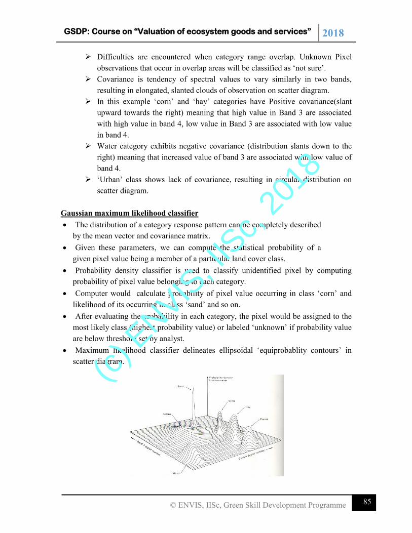
GSDP: Course on “Valuation of ecosystem goods and services” 2018
85 © ENVIS, IISc, Green Skill Development Programme
Difficulties are encountered when category range overlap. Unknown Pixel
observations that occur in overlap areas will be classified as ‘not sure’.
Covariance is tendency of spectral values to vary similarly in two bands,
resulting in elongated, slanted clouds of observation on scatter diagram.
In this example ‘corn’ and ‘hay’ categories have Positive covariance(slant
upward towards the right) meaning that high value in Band 3 are associated
with high value in band 4, low value in Band 3 are associated with low value
in band 4.
Water category exhibits negative covariance (distribution slants down to the
right) meaning that increased value of band 3 are associated with low value of
band 4.
‘Urban’ class shows lack of covariance, resulting in circular distribution on
scatter diagram.
Gaussian maximum likelihood classifier
The distribution of a category response pattern can be completely described
by the mean vector and covariance matrix.
Given these parameters, we can compute the statistical probability of a
given pixel value being a member of a particular land cover class.
Probability density classifier is used to classify unidentified pixel by computing
probability of pixel value belonging to each category.
Computer would calculate probability of pixel value occurring in class ‘corn’ and
likelihood of its occurring in class ‘sand’ and so on.
After evaluating the probability in each category, the pixel would be assigned to the
most likely class (highest probability value) or labeled ‘unknown’ if probability value
are below threshold set by analyst.
Maximum likelihood classifier delineates ellipsoidal ‘equiprobablity contours’ in
scatter diagram.
(c) E
NVIS, I
ISc,
2018
GSDP: Course on “Valuation of ecosystem goods and services” 2018
86 © ENVIS, IISc, Green Skill Development Programme
Bayesian classifier
Analyst determines ‘a priori probability’ or anticipated likelihood of
occurrence for each class in a given scene.
When classifying a pixel, probability of occurring ‘sand’ category might be
weighted lightly and more likely ‘urban’ class weighted heavily.
Drawback
Large number of computations required to classify each pixel.
Slower computationally.
Graphical representation of Spectral response Patterns
Distribution of training area response patterns can be graphically displayed in
many formats.
Histogram output is important when maximum likelihood classifier is used, it
provides a visual check on normality of spectral response distributions.
Quantitative expressions of category separation
A measure of statistical separation between category response patterns can be
computed for all pairs of classes and can be presented in form of matrix.
Self classification of training set data-
Classifying training set pixels.
Preliminary classification is only training set models (rather than full scene) is
made to determine what percentage of training set pixels are actually
classified as expected.
These percentages are actually shown in the form of error matrix.
Error matrix shows how well a classifier can classify training areas.
Training areas are usually good, homogeneous example of each cover type
can be expected to classify accurately than less pure that are found elsewhere
in the scene.
Interactive Preliminary classification
Training data are useful in classification of full scene.
Preliminary classification with computationally efficient algorithm.
Representative subscene classification
(c) E
NVIS, I
ISc,
2018
GSDP: Course on “Valuation of ecosystem goods and services” 2018
87 © ENVIS, IISc, Green Skill Development Programme
An image analyst will perform classification of representative subset of
full scene to be classified.
Unsupervised Classification
Classes that results are spectral classes
Analyst must compare classified data with some form of reference data.
Natural spectral groupings in the data can be visually identified by plotting
scatter diagram.
Classifier identifies distinct spectral classes present in image data.
There are numerous clustering algorithms that can be used to determine
natural spectral groupings present in the data set.
Unsupervised classification is the use of algorithms that incorporate
sensitivity to image ‘texture’ or ‘roughness’.
Texture defined by multidimensional variance observed in moving window
passed through image. (3X3 window).
Analyst set a variance threshold below which is considered smooth
homogenous and above which is considered rough heterogeneous.
Hybrid classification
Supervised training areas are located in regions of homogeneous cover type.
Unsupervised training areas are chosen to contain numerous cover types at
various locations throughout a scene.
Particularly valuable in analyses where there is variability in the spectral response
patterns for individual cover.
Classification of mixed Pixel
Lower resolution sensor operating at higher altitude might focus on same field yet
having its field of view occupied by mixture of soybean leaves, bare soil and
grass.
Presents a different problem for image classification since their spectral
characteristics are not representative of single land cover type.
Spectral Mixture Analysis
Range of techniques wherein mixed spectral signatures are compared to a set of
pure reference spectra.
Provides useful information at sub pixel level, since multiple land cover can be
detected within single pixel.
(c) E
NVIS, I
ISc,
2018
GSDP: Course on “Valuation of ecosystem goods and services” 2018
88 © ENVIS, IISc, Green Skill Development Programme
Linear mixture
Input to linear mixture model consists of single observed spectral signatures for
each pixel in an image.
Pure reference spectral signatures are referred as end members because they
represent cases where hundred percent of sensor’s field of view is occupied by
single cover type.
Sum of fractional proportions of end members included in a Pixel must be equal
to 1.
A given spectral band λ the observed DN λ for each pixel represents the sum of
DNs that would be obtained from Pixel that is completely covered by a given end
member weighted by fraction occupied by that member plus some unknown error.
Fuzzy classification
Membership grade values are assigned that describe how close a pixel
measurement is to means of all measurement.
Fuzzy Supervised classification
Fuzzy mean vectors and covariance matrices are developed from statistically
weighted training data.
Instead of delineating training areas that are purely homogeneous, a combination
of pure and mixed training site may be used.
Known mixtures of various feature types define fuzzy training class weight.
A classified pixel is weighted is assigned a membership grade with respect to
its membership in each information class.
Vegetation classification include pixel with grade 0.68 for class ‘forest’, 0.29 for
‘street’.
THE OUTPUT STAGE
Graphic Products
Tabular Data
Digital Information Files
Post classification smoothing
Classified data manifest salt and pepper due to inherent spectral variability
encountered by the classifier when applied on pixel by pixel basis.
Application of majority filter
(c) E
NVIS, I
ISc,
2018
GSDP: Course on “Valuation of ecosystem goods and services” 2018
89 © ENVIS, IISc, Green Skill Development Programme
A moving window is passed through the classified data set and majority of
classes within the window is determined.
If centre pixel in the window is not a majority class, its identity is changed to
majority class.
If there is no majority class in the window identity of center pixel is not
changed.
As window progresses through the data set, original class codes are
continually used not the labels as modified from previous window positions.
Major filters can incorporate some form of class / spatial weighting function.
Certain algorithms can preserve the boundaries between land cover regions
and involve user –specified minimum area of any given land cover that would
be maintained in the smoothed output.
Classification Accuracy Assessment
Classification error matrix
Compare on category by category basis, the relationship between known
reference data (ground truth).
Such matrices are square, with number of rows and columns equal to the
number of categories where classified accuracy is being assessed.
Several characteristics about classification performance are being expressed
by error matrix.
Sample considerations
Test areas are area of representative, uniform land cover that is different
from and considerably more extensive than training areas.
The accuracies obtained in these areas represent at least first
approximation to classification performance through out the scene.
Being homogeneous test areas might not provide valid indication of
classification accuracy at individual pixel level of land cover variability.
Random sampling
Collections of remote data for large sample of randomly distributed points
are often difficult and costly.
Validity of random sampling depends on ability to register reference data
to image data.
Simple random sampling tends to under sample small but important area.
Stratified random sampling where each land cover category may be
considered stratum is frequently used in each class.
(c) E
NVIS, I
ISc,
2018
GSDP: Course on “Valuation of ecosystem goods and services” 2018
90 © ENVIS, IISc, Green Skill Development Programme
Change detection process
Post classification comparison
Two dates of imagery are independently classified and registered.
An algorithm can be employed to determine those pixels with a change in
classification between dates.
Accuracy of such procedures depends upon accuracy of each of independent
classifications used in the analysis.
Classification of multitemporal data sets
Single classification is performed on a combined data set for two dates of
interest.
Principal component analysis
Used to analyze multi date image composites for change detection process.
Two or more images are registered to from new multiband image containing
all bands for each date.
It s often difficult to interpret and identify specific nature of changes involved.
Temporal image ratioing
Computing ratio of data from two dates of imaging.
Ratio of areas of no change tends towards 1 and areas of change will have higher
or lower ratio value.
Change vector analysis
Change detection procedure that is conceptual extension of image differencing.
Change verses no change binary mask to guide multidate classification
Traditional classification of one image as reference (time 1).
One of the spectral bands from this date (time 2).
This two-band dataset is analyzed using one of the algebraic operations
(example image differencing and ratioing).
Threshold is set to separate areas that have changed between data’s from those
that have not.
This mask is only applied to multiband image acquired at time 2 and only
areas of change are classified for time 2.
Hyper spectral Image Analysis
Provides vast information about physical and chemical composition of surface
under observation as well as insight into characteristics of atmosphere sensor and
the surface.
(c) E
NVIS, I
ISc,
2018
GSDP: Course on “Valuation of ecosystem goods and services” 2018
91 © ENVIS, IISc, Green Skill Development Programme
Disadvantage-
Poor signal to noise concentration
Increased susceptibility to effects of unwanted atmospheric interference.
Atmospheric correction of hyper spectral Images
The magnitude of absorption will vary from place to place and from time to time
depending on concentration and particle sizes of various atmospheric constituents.
‘raw’ radiance value observed by hyper spectral sensor cannot be directly
compared to laboratory spectra or remotely sensed hyper spectral imagery
acquired at other time or places.
Hyper image analysis techniques
Once a hyper spectral image has been corrected for effects of atmospheric
absorption and scattering reflectance “signatures” of each pixel can be compared
to previously acquired spectra for known material types.
Spectrum ratioing consists of dividing every reflectance value in the reference
spectrum by corresponding value in image spectrum.
If the average deviation from 1.0 across all wavelengths falls within some small
levels of tolerance, image spectrum for that pixel is considered to match the
reference spectrum.
Spectral angle mapping (SAM)
Observed reflectance spectrum can be considered as vector in multi dimensional
space, where the number of dimensions equals the number of spectral bands.
If the overall illumination increases or decreases the length of the vector increases
or decreases but angular orientation will remain constant.
DATA MERGING AND GIS INTEGRATION
Many applications of digital image processing are enhanced through the merger
of multiple data sets covering the same geographical area.
Multitemporal Data Merging – combining images of the same area taken
on more than one date to create a product useful for visual interpretation.
Change Detection Procedures – involves the use of land cover change
between dates of imaging.
(c) E
NVIS, I
ISc,
2018
GSDP: Course on “Valuation of ecosystem goods and services” 2018
92 © ENVIS, IISc, Green Skill Development Programme
Chapter 4: Basic Data Models
GIS depicts the real world through models involving geometry, attributes, relations, and
data quality. In this chapter, the realization of models is described, with the emphasis on
geometric spatial information, attributes, and relations. Spatial information is presented
in two ways: as vector data in the form of points, lines, and areas (polygons); or as grid
data in the form of uniform, systematically organized cells. Geometric presentations are
commonly called digital maps. Strictly speaking, a digital map would be peculiar because
it would comprise only numbers (digits). By their very nature, maps are analog, whether
they are drawn by hand or machine, or whether they appear on paper or displayed on a
screen. Technically speaking, GIS does not produce digital maps—it produces analog
maps from digital map data. Nonetheless, the term digital map is now widely used that
the distinction is well understood.
Vector Data Model: The basis of the vector model is the assumption that the real
world can be divided into clearly defined elements where each element consists an
identifiable object with its own geometry of points, lines, or areas (Figure 4.1). In
principle, every point on a map and every point in the terrain it represents is uniquely
located using two or three numbers in a coordinate system, such as in the northing,
easting, and elevation Cartesian coordinate system. On maps, coordinate systems are
commonly displayed in grids with location numbers along the map edges. On the ground,
coordinate systems are imaginary, yet marked out by survey control stations. Data usually
may be transformed from one coordinate system to another. With few exceptions, digital
representations of spatial information in a vector model are based on individual points
and their coordinates. The exceptions include cases where lines or parts of lines (e.g.,
those representing roads or property boundaries) may be described by mathematical
functions, such as those for circles or parabolas. In these cases, GIS data include equation
parameters: for example, the radii of the circles used to describe parts of lines. Together
with the coordinate data, instructions are entered as to which points in a line are
unconnected and which are connected. These instructions can subsequently be used to
create lines and polygons and to trigger “pen up” and “pen down” functions in drawing.
(c) E
NVIS, I
ISc,
2018
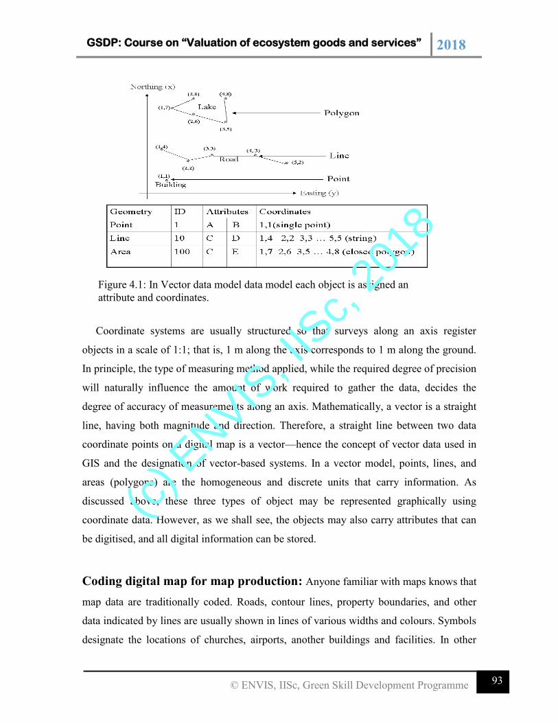
GSDP: Course on “Valuation of ecosystem goods and services” 2018
93 © ENVIS, IISc, Green Skill Development Programme
Coordinate systems are usually structured so that surveys along an axis register
objects in a scale of 1:1; that is, 1 m along the axis corresponds to 1 m along the ground.
In principle, the type of measuring method applied, while the required degree of precision
will naturally influence the amount of work required to gather the data, decides the
degree of accuracy of measurements along an axis. Mathematically, a vector is a straight
line, having both magnitude and direction. Therefore, a straight line between two data
coordinate points on a digital map is a vector—hence the concept of vector data used in
GIS and the designation of vector-based systems. In a vector model, points, lines, and
areas (polygons) are the homogeneous and discrete units that carry information. As
discussed above, these three types of object may be represented graphically using
coordinate data. However, as we shall see, the objects may also carry attributes that can
be digitised, and all digital information can be stored.
Coding digital map for map production: Anyone familiar with maps knows that
map data are traditionally coded. Roads, contour lines, property boundaries, and other
data indicated by lines are usually shown in lines of various widths and colours. Symbols
designate the locations of churches, airports, another buildings and facilities. In other
Figure 4.1: In Vector data model data model each object is assigned an
attribute and coordinates.
(c) E
NVIS, I
ISc,
2018
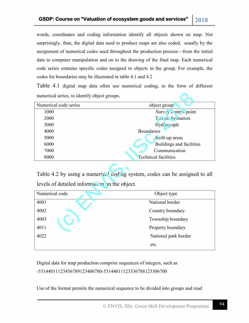
GSDP: Course on “Valuation of ecosystem goods and services” 2018
94 © ENVIS, IISc, Green Skill Development Programme
words, coordinates and coding information identify all objects shown on map. Not
surprisingly, than, the digital data used to produce maps are also coded, usually by the
assignment of numerical codes used throughout the production process—from the initial
data to computer manipulation and on to the drawing of the final map. Each numerical
code series contains specific codes assigned to objects in the group. For example, the
codes for boundaries may be illustrated in table 4.1 and 4.2
Table 4.1 digital map data often use numerical coding, in the form of different
numerical series, to identify object groups.
Numerical code series object group
1000 Survey control point
2000 Terrain formation
3000 Hydrograph
4000 Boundaries
5000 Built-up areas
6000 Buildings and facilities
7000 Communication
8000 Technical facilities
Table 4.2 by using a numerical coding system, codes can be assigned to all
levels of detailed information on the object.
Numerical code Object type
4001 National border
4002 Country boundary
4003 Township boundary
4011 Property boundary
4022 National park border
etc.
Digital data for map production comprise sequences of integers, such as
-53144011123456789123406780-53144011123336788123306700
Use of the format permits the numerical sequence to be divided into groups and read
(c) E
NVIS, I
ISc,
2018
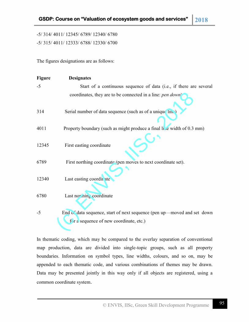
GSDP: Course on “Valuation of ecosystem goods and services” 2018
95 © ENVIS, IISc, Green Skill Development Programme
-5/ 314/ 4011/ 12345/ 6789/ 12340/ 6780
-5/ 315/ 4011/ 12333/ 6788/ 12330/ 6700
The figures designations are as follows:
Figure Designates
-5 Start of a continuous sequence of data (i.e., if there are several
coordinates, they are to be connected in a line: pen down)
314 Serial number of data sequence (such as of a unique line)
4011 Property boundary (such as might produce a final line width of 0.3 mm)
12345 First easting coordinate
6789 First northing coordinate (pen moves to next coordinate set).
12340 Last easting coordinate
6780 Last northing coordinate
-5 End of data sequence, start of next sequence (pen up—moved and set down
for a sequence of new coordinate, etc.)
In thematic coding, which may be compared to the overlay separation of conventional
map production, data are divided into single-topic groups, such as all property
boundaries. Information on symbol types, line widths, colours, and so on, may be
appended to each thematic code, and various combinations of themes may be drawn.
Data may be presented jointly in this way only if all objects are registered, using a
common coordinate system.
(c) E
NVIS, I
ISc,
2018
GSDP: Course on “Valuation of ecosystem goods and services” 2018
96 © ENVIS, IISc, Green Skill Development Programme
Coding digital data for GIS
Point objects may easily be realized in a database because a given number of attributes
and coordinates is associated with each point (Figure 4.1). Line and polygon objects are
more difficult to realize in a database because of the variation in the number of points
composing them. A line or a polygon may comprise two points or 2000 or more points,
depending on the extent of the line and the complexity of the area, which is delineated by
a boundary line that begins and ends at the same point. Object spatial information and
object attributes are often stored in different databases to ease the manipulation of lines
and areas, but in some systems they are stored together. As pivotal attributes are often
available in existing computer memory files, dividing the databases conserves memory
by precluding duplicate storage of the same data. The separate storage of attribute and
spatial information data requires that all objects in the attribute tables be associated with
the corresponding spatial information. This association is achieved by inserting spatially
stable and relevant attribute data or codes form the attribute table into the special
information, or vice-versa. In other words, identical objects have the same identities in
both databases. The identity (ID) codes used to label and connect spatial information and
attribute table data are most often numerical, but may be alphanumerical. Typical identity
codes include building numbers, property numbers and addresses. If the data are ordered
in a manuscript map, each object may be assigned a serial number used in both the spatial
information and the attribute databases. Polygons for vegetation mapping can, for
example, be numbered from 1 onward, while pipes, manholes, and so on, are usually
numbered according to an administrative system. ID codes allow differentiation between
objects, whereas theme codes allow differentiation between different groups of objects.
In theory, identity codes and thematic codes are both attributive data. However, they are
very closely tied to geometry and are therefore often treated as such, as described above.
(c) E
NVIS, I
ISc,
2018
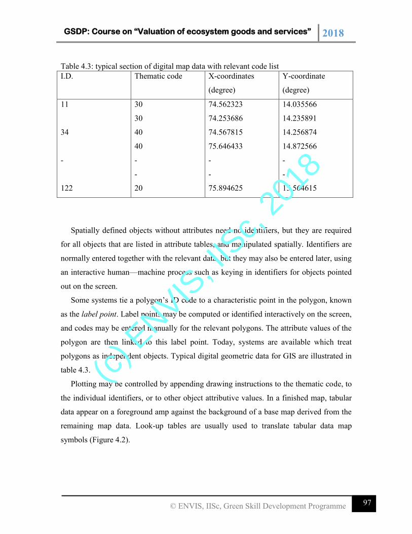
GSDP: Course on “Valuation of ecosystem goods and services” 2018
97 © ENVIS, IISc, Green Skill Development Programme
Table 4.3: typical section of digital map data with relevant code list
Spatially defined objects without attributes need no identifiers, but they are required
for all objects that are listed in attribute tables, and manipulated spatially. Identifiers are
normally entered together with the relevant data, but they may also be entered later, using
an interactive human—machine process such as keying in identifiers for objects pointed
out on the screen.
Some systems tie a polygon’s ID code to a characteristic point in the polygon, known
as the label point. Label points may be computed or identified interactively on the screen,
and codes may be entered manually for the relevant polygons. The attribute values of the
polygon are then linked to this label point. Today, systems are available which treat
polygons as independent objects. Typical digital geometric data for GIS are illustrated in
table 4.3.
Plotting may be controlled by appending drawing instructions to the thematic code, to
the individual identifiers, or to other object attributive values. In a finished map, tabular
data appear on a foreground amp against the background of a base map derived from the
remaining map data. Look-up tables are usually used to translate tabular data map
symbols (Figure 4.2).
I.D. Thematic code X-coordinates
(degree)
Y-coordinate
(degree)
11
34
-
122
30
30
40
40
-
-
20
74.562323
74.253686
74.567815
75.646433
-
-
75.894625
14.035566
14.235891
14.256874
14.872566
-
-
15.564615
(c) E
NVIS, I
ISc,
2018
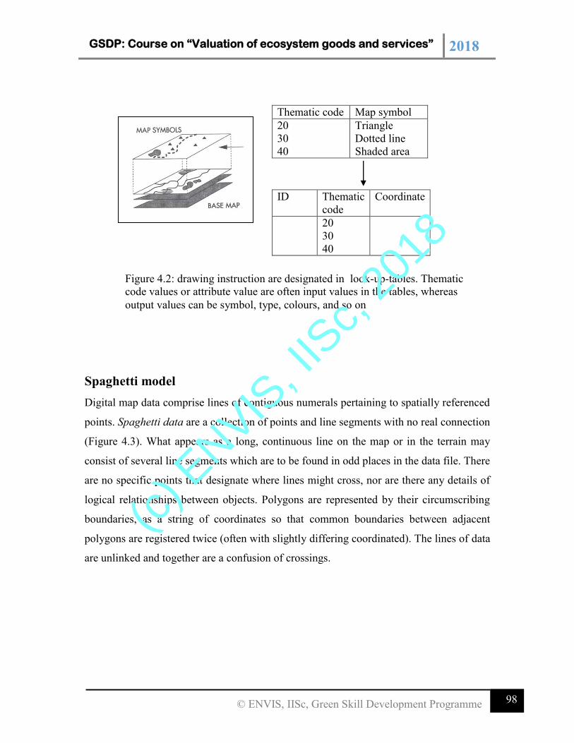
GSDP: Course on “Valuation of ecosystem goods and services” 2018
98 © ENVIS, IISc, Green Skill Development Programme
Spaghetti model
Digital map data comprise lines of contiguous numerals pertaining to spatially referenced
points. Spaghetti data are a collection of points and line segments with no real connection
(Figure 4.3). What appears as a long, continuous line on the map or in the terrain may
consist of several line segments which are to be found in odd places in the data file. There
are no specific points that designate where lines might cross, nor are there any details of
logical relationships between objects. Polygons are represented by their circumscribing
boundaries, as a string of coordinates so that common boundaries between adjacent
polygons are registered twice (often with slightly differing coordinated). The lines of data
are unlinked and together are a confusion of crossings.
Thematic code Map symbol
20
30
40
Triangle
Dotted line
Shaded area
ID Thematic
code
Coordinate
20
30
40
Figure 4.2: drawing instruction are designated in look-up-tables. Thematic
code values or attribute value are often input values in the tables, whereas
output values can be symbol, type, colours, and so on
(c) E
NVIS, I
ISc,
2018
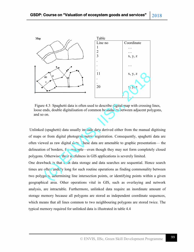
GSDP: Course on “Valuation of ecosystem goods and services” 2018
99 © ENVIS, IISc, Green Skill Development Programme
Unlinked (spaghetti) data usually include data derived either from the manual digitising
of maps or from digital photogrammetric registration. Consequently, spaghetti data are
often viewed as raw digital data. These data are amenable to graphic presentation— the
delineation of borders, for example—even though they may not form completely closed
polygons. Otherwise, their usefulness in GIS applications is severely limited.
One drawback is that both data storage and data searches are sequential. Hence search
times are often unduly long for such routine operations as finding commonality between
two polygons, determining line intersection points, or identifying points within a given
geographical area. Other operations vital in GIS, such as overlaying and network
analysis, are intractable. Furthermore, unlinked data require an inordinate amount of
storage memory because all polygons are stored as independent coordinate sequences,
which means that all lines common to two neighbouring polygons are stored twice. The
typical memory required for unlinked data is illustrated in table 4.4
Table
Line no
1
2
3
.
.
.
11
.
.
20
Coordinate
…
…
x, y, z
…
x, y, z
x, y, z
Figure 4.3: Spaghetti data is often used to describe digital map with crossing lines,
loose ends, double digitalisation of common boundaries between adjacent polygons,
and so on.
(c) E
NVIS, I
ISc,
2018
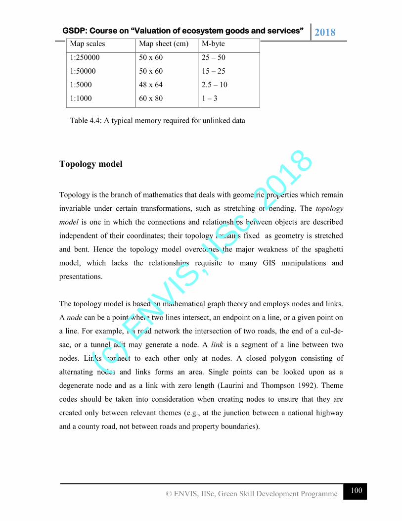
GSDP: Course on “Valuation of ecosystem goods and services” 2018
100 © ENVIS, IISc, Green Skill Development Programme
Topology model
Topology is the branch of mathematics that deals with geometric properties which remain
invariable under certain transformations, such as stretching or bending. The topology
model is one in which the connections and relationships between objects are described
independent of their coordinates; their topology remains fixed as geometry is stretched
and bent. Hence the topology model overcomes the major weakness of the spaghetti
model, which lacks the relationships requisite to many GIS manipulations and
presentations.
The topology model is based on mathematical graph theory and employs nodes and links.
A node can be a point where two lines intersect, an endpoint on a line, or a given point on
a line. For example, I a road network the intersection of two roads, the end of a cul-de-
sac, or a tunnel adit may generate a node. A link is a segment of a line between two
nodes. Links connect to each other only at nodes. A closed polygon consisting of
alternating nodes and links forms an area. Single points can be looked upon as a
degenerate node and as a link with zero length (Laurini and Thompson 1992). Theme
codes should be taken into consideration when creating nodes to ensure that they are
created only between relevant themes (e.g., at the junction between a national highway
and a county road, not between roads and property boundaries).
Table 4.4: A typical memory required for unlinked data
Map scales Map sheet (cm) M-byte
1:250000
1:50000
1:5000
1:1000
50 x 60
50 x 60
48 x 64
60 x 80
25 – 50
15 – 25
2.5 – 10
1 – 3
(c) E
NVIS, I
ISc,
2018
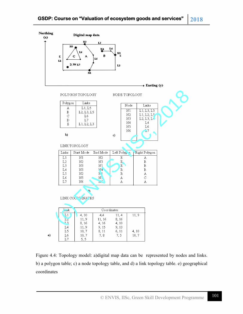
GSDP: Course on “Valuation of ecosystem goods and services” 2018
101 © ENVIS, IISc, Green Skill Development Programme
Figure 4.4: Topology model: a)digital map data can be represented by nodes and links.
b) a polygon table; c) a node topology table, and d) a link topology table. e) geographical
coordinates
(c) E
NVIS, I
ISc,
2018
GSDP: Course on “Valuation of ecosystem goods and services” 2018
102 © ENVIS, IISc, Green Skill Development Programme
Unique identities are assigned to all links, nodes, and polygons, and attribute data
describing connections are associated with all identities. Topology can therefore be
described in three tables (figure 4.4):The polygon topology table lists the links
comprising all polygons, each of which is identified by a number.
1. The node topology table lists the links that meet at each node.
2. the link topology table lists the nodes on which each link terminates and the
polygons on the right and left of each link, with right and left defined in the
direction from a designated start node to a finish code. The system creates these
tables automatically.
A table with point coordinates to the links ties these features to the real world and permits
computations of distances, areas, intersections, and other numerical parameters. The
geometry of the objects is stored in its own subordinate table (see Figure 4.4). Numerous
spatial analyses may then be performed, including:
Overlaying
Network analyses
Contiguity analyses
Connectivity analyses
Topological attribute data may be used directly in contiguity analyses and other
manipulations with no intervening, time-consuming geometric operations.
Once the topology has been created, a map can be plotted with solid colours. This is
not possible with spaghetti data. Thematic layers of topological data can also be used to
steer the plotting sequence. The sequence influences what becomes visible on the map.
For example, a green area superimposed on a white house will render the house invisible
on the map (unless the house creates a window in the area).
Topology requires that all lines should be connected, all polygons closed, and all
loose ends removed. Even gaps as small as 0.001 mm may be excessive, so errors should
(c) E
NVIS, I
ISc,
2018
GSDP: Course on “Valuation of ecosystem goods and services” 2018
103 © ENVIS, IISc, Green Skill Development Programme
be removed either prior to or during the compilation of topological tables.
A function known as snap can also be used in digitisation. Using the snap function
with a defined tolerance of, say, 1 mm, a search can be carried out around the end of a
line or around an existing point which is assumed to have the same coordinates as the last
point registered. When this point is found, the two points will be snapped together to
form a common node, thereby closing the polygon. The same procedure can be carried
out automatically on existing data. A node can also be created in existing data by
calculating the point of intersection between lines. Meaningless loose ends can be
removed by testing with a given minimum length.
Topological information permits automatic verification of data consistency to detect
such errors as the incomplete closing of polygons during the encoding process. The graph
theory contains formulas for the calculation of such data errors. There has to be a fixed
relationship between the number of nodes, lines, and polygons in one data set. A run-
through of the data in positive and negative directions will produce the same result.
The topological model has a few drawbacks. The computational time required to
identify all nodes may be relatively long. Uncertainties and errors may easily arise in
connection with the closing of polygons and formation of nodes in complex networks
(such as in road interchanges). Operators must solve such problems. When raw data are
entered and existing data updated, new nodes must be computed and the topology tables
brought up to date.
Topological data may require a longer plotting time than spaghetti data because of
the separation of lines into nodes and links. However, the overall advantages of the
topology model over the spaghetti model make it the prime choice in most GISs. Today,
efficient software and faster computers enable topology to be established on-the-fly; thus
the disadvantages of topological data as compared to spaghetti data have become less
important.
Here it suffices to say that usually. Map data are not stored in a contiguous unit, but
(c) E
NVIS, I
ISc,
2018
GSDP: Course on “Valuation of ecosystem goods and services” 2018
104 © ENVIS, IISc, Green Skill Development Programme
rather, divided into lesser units that are stored according to a selected structure. This
structure may be completely invisible to the user, but its effects, such as rapid screen
presentation of a magnified portion of a map, are readily observable.
Data Compression
The amount of computer resources (memory and storage space) needed can be reduced
by using data compression techniques. Most of these automatic techniques are based on
removing points from continuous lines (contour lines, etc.). Good data compression
techniques, therefore are those that preserve the highest possible degree of geometric
accuracy. The most basic technique involves the elimination of repetitive characters: for
example, the first character of all coordinates along a particular axis. The repetitive
character needs to be entered only once; subsequently, it may be added to each set of
coordinates. The particular technique has no effect on the geometry.
There are other automatic methods of removing points. One simple means is to keep only
every nth point on the line. The lower the value of n, the greater the number of points that
will be removed. This method does not take into account geometric accuracy; however,
this can be compensated for by testing the curvature of the line. One method is to draw a
straight line between the first and last points on a curved stretch of line and to calculate
the orthogonal distance from each point on the curve line below the straight one. Points
that are closer than a given distance from the straight line will be removed. The endpoint
of the straight line is then moved to the point with the greatest distance and the same
procedure for removing points is repeated. This continues until all the relevant points are
removed. This method is known as the Douglas-Peucker algorithm.
Points of little or no value in describing a line may be eliminated by moving a corridor
step by step along a line and deleting points that are closer to the neighbouring point than
a given value or where the vectors create an angle that is smaller than the given value.
Contours and other lines can also be replaced with mathematical functions, such as
straight lines, parabolas, and polynomials. A spline function comprises segments of
polynomials joined smoothly at a finite number of points so as to approximate a line. A
(c) E
NVIS, I
ISc,
2018
GSDP: Course on “Valuation of ecosystem goods and services” 2018
105 © ENVIS, IISc, Green Skill Development Programme
spline function can involve several polynomials to build a complex shape. It has been
reported that a spline function representing nautical chart data has reduced data volume
by 95%.
The amount of memory required to store a given amount of data often depends on the
format in which data are entered. Some formats contain more administrative routines than
others, some have vacant space. Thus, the gross volumes stored are frequently related to
format.
Storing vector data
The manner in which digital map data are stored in a record is determined by a format, a
set of instructions specifying how data are arranged in fields. The latter are groups of
characters or words, which, in turn, are treated as units of data. The format stipulates how
the computer will read data into the fields: total number of fields specified, number of
characters permissible in each field, number of spaces between fields, which fields are
numeric and which are text, and so on.
He information content of the data is designated not in the format but ancillary to it, for
example, in a heading. Typical specifications for information content might include field
assignments, such as the point number in the first field, the thematic code in the second,
easting in the third, northing in the fourth, and elevation in the fifth. The meanings of the
numeric codes used must also be given. The spaghetti data are stored in simple file
structure and in order in which the data have been registered.
Users of conventional maps know the frustrations of extracting information from maps
produced by various agencies using differing map sheet series, varying scales and
coordinate systems, and frequently, different symbols for the same themes. Moreover, the
graphic version of Murphy’s law dictates that the necessary information is all too often
located in the corners where four adjoining map sheets meet.
Database storage of cartographic data can overcome these problems because it involves
(c) E
NVIS, I
ISc,
2018
GSDP: Course on “Valuation of ecosystem goods and services” 2018
106 © ENVIS, IISc, Green Skill Development Programme
standardization of data through common reference systems and uniform formats.
Cartographic data from various sources can, with few limitations, be combined. The
results are then independent of map sheet series and scales.
Standardized storage makes the presentation of data compiled from dissimilar sources
much easier. For example, uniform storage formats permit the combination of
telecommunications administration network data with property survey data, or of
geological information from 1: 50,000 scale maps with vegetation data from 1: 20,000
scale maps.
Digital map data are stored in databases, the computerised equivalent of conventional
file drawers and cabinets. Although data entries in a database can be updated far more
rapidly than data printed on map sheets on file, the information is found more quickly
from map sheets than by searching in a database. This is because a single map sheet
contains an enormous amount of information, usually equivalent to 100,000 or more sets
of coordinates. A sequential computer search of 100,000 items in a database is slow even
for the most powerful computers in comparison with a quick visual scan of a map sheet.
Therefore, “smart” programs known as database management systems (DBMSs) have
been compiled to maintain, access, and manipulate databases. The various DBMSs differ
primarily in the ways in which data are organized. Their selection and use are vital in GIS
applications because they determine the speed and flexibility with which data may be
accessed.
It is usual to split topological data into different thematic layers to simplify storage and to
improve access to data. This division is done so that no overlap occurs between polygons
within each thematic layer. For example, property boundaries are stored in one layer
while other data overlapping the property, such as roads, buildings, and vegetation
boundaries, are stored in another. The disadvantage of this system is that common lines
between objects (e.g., roads and properties) that are stored in different layers have to be
removed several times. This problem can be avoided by using object-based storage.
(c) E
NVIS, I
ISc,
2018
GSDP: Course on “Valuation of ecosystem goods and services” 2018
107 © ENVIS, IISc, Green Skill Development Programme
Comments on spaghetti and topology models
When digitising lines such as those on land-use maps, the borders of surfaces are
digitised both as spaghetti data and as separate objects. When creating topology, this
model is converted to a layer model. The discussion of spaghetti and topology is very
much based on the assumption that a class of area entities is always a tiling of the plane
in which every point lies in exactly one polygon. However, the problems related to
spaghetti and topology have changed somewhat during recent years with the advent of
new GIS software which treats polygons as independent objects that may overlap and
need not fill the plane, and with systems permitting shapes. Many of the traditional
arguments for area coverage/ layer model and use of topology are based on the
assumption of needing to avoid computation. New and more powerful computers
eliminate the need for reduction in calculation time. Today, topology can easily be built
on-the-fly.
Raster data models
Raster data are applied in at least four ways:
1. Modelling describing the real world
2. Digital maps scans of exiting maps
3. Compiling digital satellite and image data
4. Automatic drawing by raster output units
In the first example, raster data are associated with selected data models of real world: in
the second and third, with compilation method, and in the fourth, with presentation
methods. The respective computer manipulation may be entered in a raster model.
Raster models
Raster model represents reality through selected surface arranged in a regular pattern.
Reality is thus generalised in terms of uniform, regular cells, which are usually
rectangular or square but may be triangular or hexagonal. The raster model is in many
ways a mathematical model, as represented by the regular cell pattern. Because square or
rectangles are often used and a pictorial view of them resembles a classic grid of squares,
(c) E
NVIS, I
ISc,
2018
GSDP: Course on “Valuation of ecosystem goods and services” 2018
108 © ENVIS, IISc, Green Skill Development Programme
it is sometimes called the grid model. Geometric resolution of the model depends on the
size of the cell. With in each cell the terrain is assumed to be flat.
The rectangular raster cells, usually of uniform size throughout a model, affect the final
drawing in two ways. First, lines that are continuous and smooth in a vector model will
become jagged, with the jag size corresponding to the cell size. Second, resolution is
constant: region with few variation are as detailed as those with major variations, and
vice versa.
The cells of a model are given in a sequence determined by a hierarchy of rows and
column in a matrix, with numbering usually starting from the upper left corner (figure
4.2). The geometric location of cell, and hence of the object it represents, is stated in
terms of its directional and column number. This identification corresponds to the
directional coordinates of the vector model. The cells are often called pixel. A pixel is the
smallest element of an image that can be processed and displayed individually. The raster
techniques used in GIS are sibling of the raster long used to facilitate the manipulation
and display of the information and consequently are suited to computerised technique.
Realizing the raster model
Raster models are created by assigning real-world values to pixels (Figure 4.5). The
assigned values comprise the attributes of the objects that the cells represent—and
because the cells themselves are in a raster, only the assigned values are stored. Values,
usually alphanumeric, should be assigned to all the pixels in a raster. Otherwise, there is
little purpose in drawing empty rows and columns in a raster.
Consider a grid of cells superimposed on the ground or on a map. Assigning the
values/ codes of the underlying objects/ features to the cells creates the model. The
approach is comprehensive because everything covered by the raster is included in the
model. Draping a ground surface in this way regards the ground or map as a plane
surface.
(c) E
NVIS, I
ISc,
2018
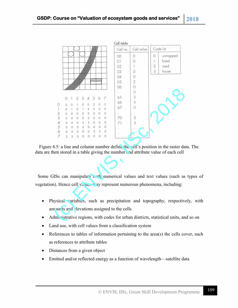
GSDP: Course on “Valuation of ecosystem goods and services” 2018
109 © ENVIS, IISc, Green Skill Development Programme
Figure 4.5: a line and column number define the cell’s position in the raster data. The
data are then stored in a table giving the number and attribute value of each cell
Some GISs can manipulate both numerical values and text values (such as types of
vegetation). Hence cell values may represent numerous phenomena, including:
Physical variables, such as precipitation and topography, respectively, with
amounts and elevations assigned to the cells
Administrative regions, with codes for urban districts, statistical units, and so on
Land use, with cell values from a classification system
References to tables of information pertaining to the area(s) the cells cover, such
as references to attribute tables
Distances from a given object
Emitted and/or reflected energy as a function of wavelength—satellite data
(c) E
NVIS, I
ISc,
2018
GSDP: Course on “Valuation of ecosystem goods and services” 2018
110 © ENVIS, IISc, Green Skill Development Programme
A single cell may be assigned only one value, so dissimilar objects and their values
must be assigned to different raster layers, each of which deals with one thematic topic
(figure 4.6). Hence in raster models as in vector models, there are thematic layers for
topography, water supply systems, land use, and soil type. However, because of the
differences in the way attribute information is manipulated, raster models usually have
more layers than those in vector models. In a vector model, attributes are assigned
directly to objects. For instance, pH value might be assigned directly to the object “lake”.
In a raster model, the equivalent assignment requires one thematic layer for the lake, in
which cells are assigned to the lake in question, and a second thematic layer for the cells
carrying the pH values. Raster databases may, therefore, contain hundreds of thematic
layers.
In practice, a single cell may cover parts of two or more objects or values. Normally,
the value assigned is that of the object taking up the greater part of the cell’s area, or of
the object at the middle of the cell, or that of an average computed for the whole of the
cells. Cell locations, defined in terms of rows and columns, may be transformed to
rectangular ground coordinates, for example, by assigning ground coordinates to the
centre of the upper left cell of a raster (cell 0, 0). If the raster is to be oriented north-
south, the columns are aligned along the northing axis and the rows along the existing
axis. The coordinates of all cell corners and centres can then be computed using the
known cell shapes and sizes.
Object relations, which in the vector model are described by topology, are only partly
inherent in the raster structure. When the row and column numbers of a cell are known,
the locations of neighbouring cells can easily be calculated. In the same way, cells
contained ii a given polygon may be located simply searching with a stipulated value. It
is much more difficult, however, to identify all the cells located on the border between
two polygons. Polygon areas are determined merely by adding up constituent cells. Some
operations, though, are more cumbersome. An example, of this is computation of a
polygon’s perimeter length, which requires a search for, and identification of, all the cells
along the polygon’s border.
(c) E
NVIS, I
ISc,
2018
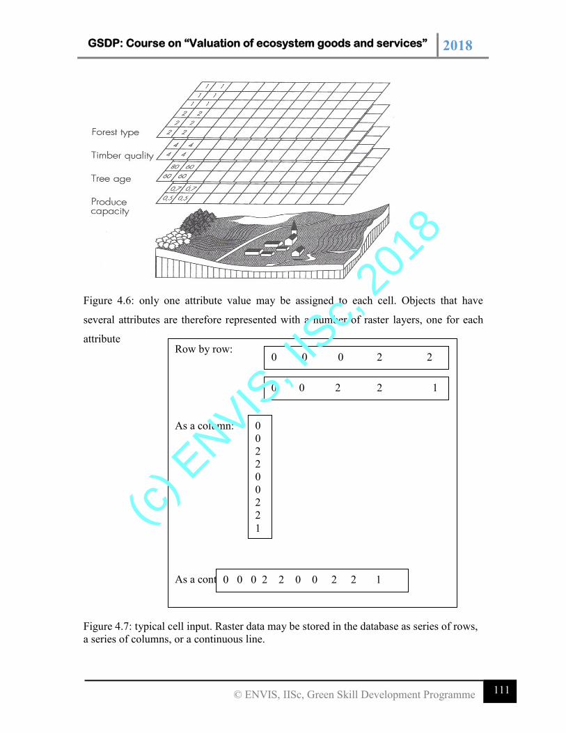
GSDP: Course on “Valuation of ecosystem goods and services” 2018
111 © ENVIS, IISc, Green Skill Development Programme
Figure 4.6: only one attribute value may be assigned to each cell. Objects that have
several attributes are therefore represented with a number of raster layers, one for each
attribute
Figure 4.7: typical cell input. Raster data may be stored in the database as series of rows,
a series of columns, or a continuous line.
Row by row:
As a column:
As a continuous line:
0 0 0 2 2
0 0 2 2 1
0
0
2
2
0
0
2
2
1
0 0 0 2 2 0 0 2 2 1
(c) E
NVIS, I
ISc,
2018
GSDP: Course on “Valuation of ecosystem goods and services” 2018
112 © ENVIS, IISc, Green Skill Development Programme
Overviews of phenomena in a given area are obtained from a raster model quickly and
easily b searching all the thematic layers for cells with the same row and column
numbers. The relevant overlay analysis is described later. Raster data are normally stored
as a matrix, as described above. However, they can also be stored in tabular form, where
each individual cell in a raster forms a line in the table (see Figure 4.7)
Coding raster data
Numerical codes and, in some systems, text codes may be assigned to cells. Cell values
are entered from word processing files, databases, or other sources in the same sequence
as they are registered (Figure 4.7). The way in which the figures are read is dictated by
format. For instance, it is essential to know the number of columns per row. Raster data
may be available from a variety of dissimilar sources, ranging from satellite data and data
entered manually to digital elevation data. Their collocation requires that cells from
differing sources and thematic layers correspond with each other. In other words, cells
having the same row and column numbers must refer to the same ground area. Various
computations may be necessary to accommodate any differences in cell shape and size.
Cells may contain values referenced to attribute tables. The cells of a thematic layer may
be coded so that their values correspond to identities in a given attribute table. Attribute
data or tabular data may be coded independently; irrespective of whether the geometry is
represented using vector data or raster data.
Compression of raster data
It the cell values of a raster model are entered in fixed matrices with rows and columns
identical to those of the registered data, only the cell values need to be stored; row and
column numbers need not. Even when only the cell values are stored, the volumes of data
can easily become unwieldy. Typical operations may involve 200 thematic layers, each
containing 5000 cells. The total number of cell values stored is thus 200 x 5000 =1
million. A land sat satellite raster image contains about 7 million pixels, a Landsat TM
image about 35 million pixels.
(c) E
NVIS, I
ISc,
2018
GSDP: Course on “Valuation of ecosystem goods and services” 2018
113 © ENVIS, IISc, Green Skill Development Programme
Various devices may be employed to reduce data volume and, consequently, storage
memory requirements. Cells of the same value are often neighbours because they pertain
to the same soil type, the same population density of an area, or other similar parameters.
Thus cells of the same value in a row may be compacted by stating the value and their
total. This type of compacting, called run-length encoding. Further compacting may be
achieved by applying the same process recursively to subsequent lines.
(c) E
NVIS, I
ISc,
2018

GSDP: Course on “Valuation of ecosystem goods and services” 2018
113 © ENVIS, IISc, Green Skill Development Programme
Housekeeping tools
From the users viewpoint the ideal GIS should include enough functions perform all
conceivable manipulations data. In practice, user needs comprise various tasks.
i). Database management system (DBMS)
ii). Query language (QL)
iii). User interface
iv). Application function and programs
Database management system
Data is the name given to the basic facts and entities such as names and numbers. Data
consists of a series of facts or statements that may have been collected, stored, processed
and / or manipulated but not have been organised or placed into context. When data is
organised, it becomes information. Information can be processed and used to draw
generalised conclusions or knowledge.
Database can be defined as ‘A collection of structured data’. The structure of the data is
independent of any particular application. A Database is a file of data structured in such
a way that it may serve a number of applications without its structure being dictated by
any one of those applications. A Database Management System is a computerised
record-keeping system that stores, maintains and provides access to information. A
Database system involves four major components Data, Hardware, Software and the
Users.
The Database Models that are been used to organise and represent the data are
1. Hierarchical Database Model,
2. Network Database Model and
3. Relational Database Model.
The Hierarchical Database Model uses one to many relationships. The parent-child
relations are employed here. This model is easy to understand and easy to update and
expand. The disadvantage of this model is that large memory is required and at times
(c) E
NVIS, I
ISc,
2018
GSDP: Course on “Valuation of ecosystem goods and services” 2018
114 © ENVIS, IISc, Green Skill Development Programme
certain attribute values should be repeated, which results in redundancy, storage and
access costs. This software uses this database model only.
The Network Database Model uses many to many relationships. The attributes are linked
from one place to another. These are interlinked within each other. The attributes can be
retrieved from another place also. The entity can have more than one parent. One member
can belong to more than one relationship. The Hierarchical and Network models are
conceptually simple but while implementing they appear to be complicated in giving the
interrelationships.
The Relational Database Model uses relations to store the data. A relational database is a
collection of tabular relations, each having a set of attributes. The data in a relation are
structured as a set of rows and is called as ‘tuples’ consisting of a list of values, one for
each attribute. An attribute has a domain, associated with it, from which its values are
drawn.
A Database Management System (DBMS) is a program that allows users to define,
manipulate and process the data in a database, in order to produce meaningful
information. DBMS is a collection of programs that enables one to store, modify and
extract information from a database. There are many types of DBMSs, ranging from
small systems that run on personal computers to huge systems that run on mainframes.
Functions of a DBMS:
To store data
To organise data
To control access to data
To protect data
Advantages of DBMS:
(c) E
NVIS, I
ISc,
2018
GSDP: Course on “Valuation of ecosystem goods and services” 2018
115 © ENVIS, IISc, Green Skill Development Programme
DBMS is not only effective for generating and maintaining a wide variety of routine
management and operating reports, but also adaptable to meeting the new and
emerging requirements of management to answer a myriad of “What if?” questions.
Data elements can be structured in a manner more suitable to their application,
allowing their retrieval with a minimum effort.
DBMS keeps redundancy of data elements to a minimum.
Application programs are independent of the changes in the database, so that their
maintenance is kept to a bare minimum.
It gives a clear picture of logical organisation of data set.
It provides data protection not only for accessing one database record at a time, but
also for preventing database access by unauthorised personnel.
It provides centralisation for multi-users.
It provides data independence.
It monitors database performance.
Centralised data reduces management problems.
Data redundancy and consistency are controllable.
Program-data interdependency is diminished.
Flexibility of data is increased.
Reduction in data redundancy.
Maintenance of data integrity and quality.
Data are self-documented or self-descriptive.
Avoidance of inconsistency.
Reduced cost of software development.
Security restrictions.
Application programs are independent of structure of DB.
Application programs share the same data.
New programs are easier and cost less to implement.
Normalization: Normalization is a process that involves eliminating problems by
decomposing the relation into two or more relations without loss of information. It is the
(c) E
NVIS, I
ISc,
2018
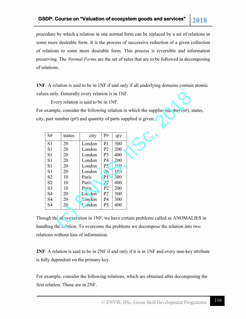
GSDP: Course on “Valuation of ecosystem goods and services” 2018
116 © ENVIS, IISc, Green Skill Development Programme
procedure by which a relation in one normal form can be replaced by a set of relations in
some more desirable form. It is the process of successive reduction of a given collection
of relations to some more desirable form. This process is reversible and information
preserving. The Normal Forms are the set of rules that are to be followed in decomposing
of relations.
1NF: A relation is said to be in 1NF if and only if all underlying domains contain atomic
values only. Generally every relation is in 1NF.
Every relation is said to be in 1NF.
For example, consider the following relation in which the supplier number (s#), status,
city, part number (p#) and quantity of parts supplied is given.
S# status city P# qty
S1
S1
S1
S1
S1
S1
S2
S2
S3
S4
S4
S4
20
20
20
20
20
20
10
10
10
20
20
20
London
London
London
London
London
London
Paris
Paris
Paris
London
London
London
P1
P2
P3
P4
P5
P6
P1
P2
P2
P2
P4
P5
300
200
400
200
100
100
300
400
200
300
300
400
Though the above relation in 1NF, we have certain problems called as ANOMALIES in
handling the relation. To overcome the problems we decompose the relation into two
relations without loss of information.
2NF: A relation is said to be in 2NF if and only if it is in 1NF and every non-key attribute
is fully dependent on the primary key.
For example, consider the following relations, which are obtained after decomposing the
first relation. These are in 2NF.
(c) E
NVIS, I
ISc,
2018
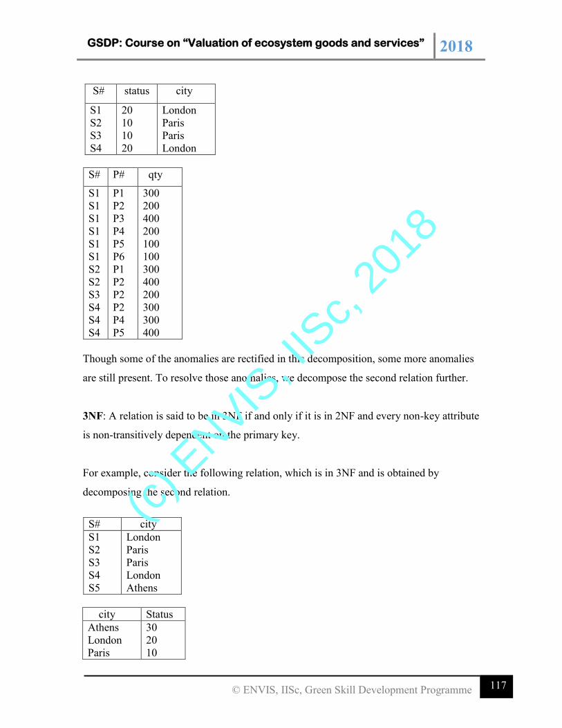
GSDP: Course on “Valuation of ecosystem goods and services” 2018
117 © ENVIS, IISc, Green Skill Development Programme
S# status city
S1
S2
S3
S4
20
10
10
20
London
Paris
Paris
London
S# P# qty
S1
S1
S1
S1
S1
S1
S2
S2
S3
S4
S4
S4
P1
P2
P3
P4
P5
P6
P1
P2
P2
P2
P4
P5
300
200
400
200
100
100
300
400
200
300
300
400
Though some of the anomalies are rectified in this decomposition, some more anomalies
are still present. To resolve those anomalies, we decompose the second relation further.
3NF: A relation is said to be in 3NF if and only if it is in 2NF and every non-key attribute
is non-transitively dependent on the primary key.
For example, consider the following relation, which is in 3NF and is obtained by
decomposing the second relation.
S# city
S1
S2
S3
S4
S5
London
Paris
Paris
London
Athens
city Status
Athens
London
Paris
30
20
10
(c) E
NVIS, I
ISc,
2018
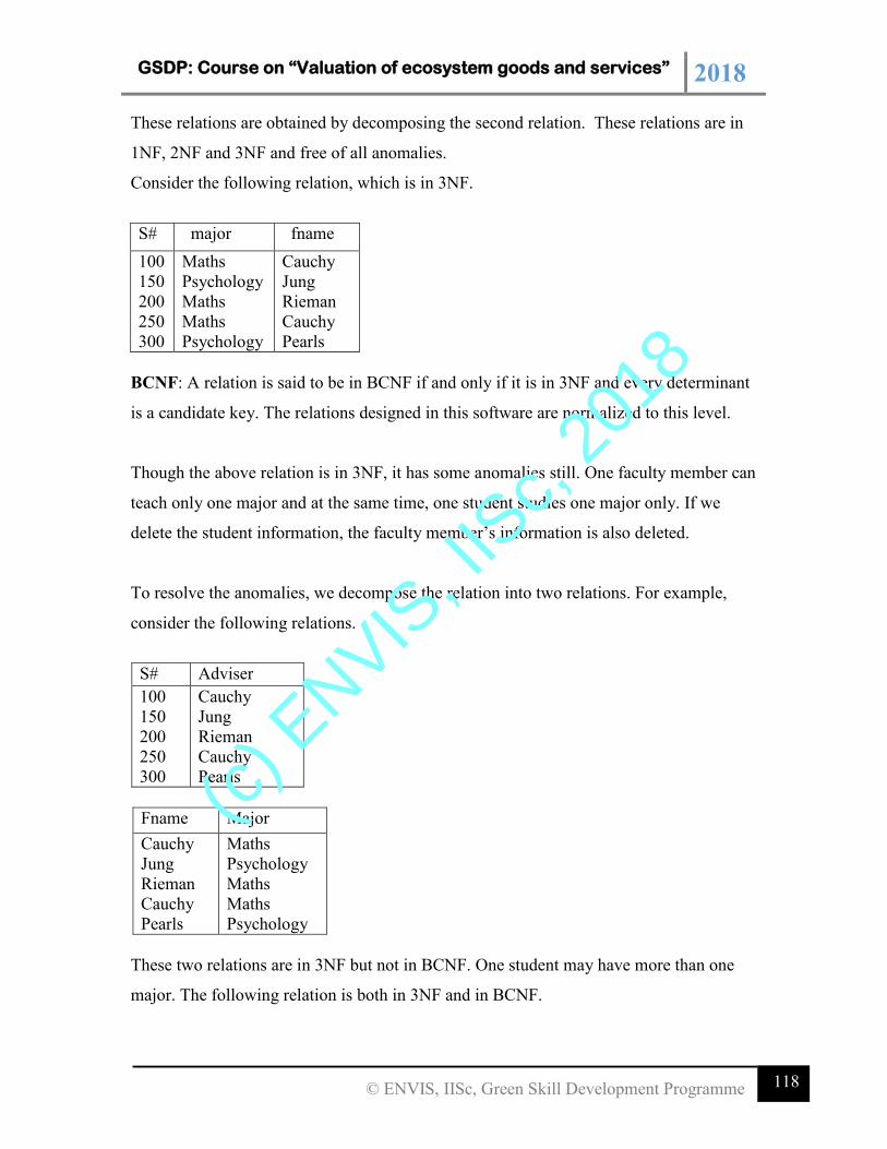
GSDP: Course on “Valuation of ecosystem goods and services” 2018
118 © ENVIS, IISc, Green Skill Development Programme
These relations are obtained by decomposing the second relation. These relations are in
1NF, 2NF and 3NF and free of all anomalies.
Consider the following relation, which is in 3NF.
S# major fname
100
150
200
250
300
Maths
Psychology
Maths
Maths
Psychology
Cauchy
Jung
Rieman
Cauchy
Pearls
BCNF: A relation is said to be in BCNF if and only if it is in 3NF and every determinant
is a candidate key. The relations designed in this software are normalized to this level.
Though the above relation is in 3NF, it has some anomalies still. One faculty member can
teach only one major and at the same time, one student studies one major only. If we
delete the student information, the faculty member’s information is also deleted.
To resolve the anomalies, we decompose the relation into two relations. For example,
consider the following relations.
S# Adviser
100
150
200
250
300
Cauchy
Jung
Rieman
Cauchy
Pearls
Fname Major
Cauchy
Jung
Rieman
Cauchy
Pearls
Maths
Psychology
Maths
Maths
Psychology
These two relations are in 3NF but not in BCNF. One student may have more than one
major. The following relation is both in 3NF and in BCNF.
(c) E
NVIS, I
ISc,
2018
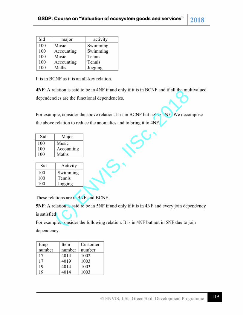
GSDP: Course on “Valuation of ecosystem goods and services” 2018
119 © ENVIS, IISc, Green Skill Development Programme
Sid major activity
100
100
100
100
100
Music
Accounting
Music
Accounting
Maths
Swimming
Swimming
Tennis
Tennis
Jogging
It is in BCNF as it is an all-key relation.
4NF: A relation is said to be in 4NF if and only if it is in BCNF and if all the multivalued
dependencies are the functional dependencies.
For example, consider the above relation. It is in BCNF but not in 4NF. We decompose
the above relation to reduce the anomalies and to bring it to 4NF.
Sid Major
100
100
100
Music
Accounting
Maths
Sid Activity
100
100
100
Swimming
Tennis
Jogging
These relations are in 4NF and BCNF.
5NF: A relation is said to be in 5NF if and only if it is in 4NF and every join dependency
is satisfied.
For example, consider the following relation. It is in 4NF but not in 5NF due to join
dependency.
Emp
number
Item
number
Customer
number
17
17
19
19
4014
4019
4014
4014
1002
1003
1003
1003
(c) E
NVIS, I
ISc,
2018
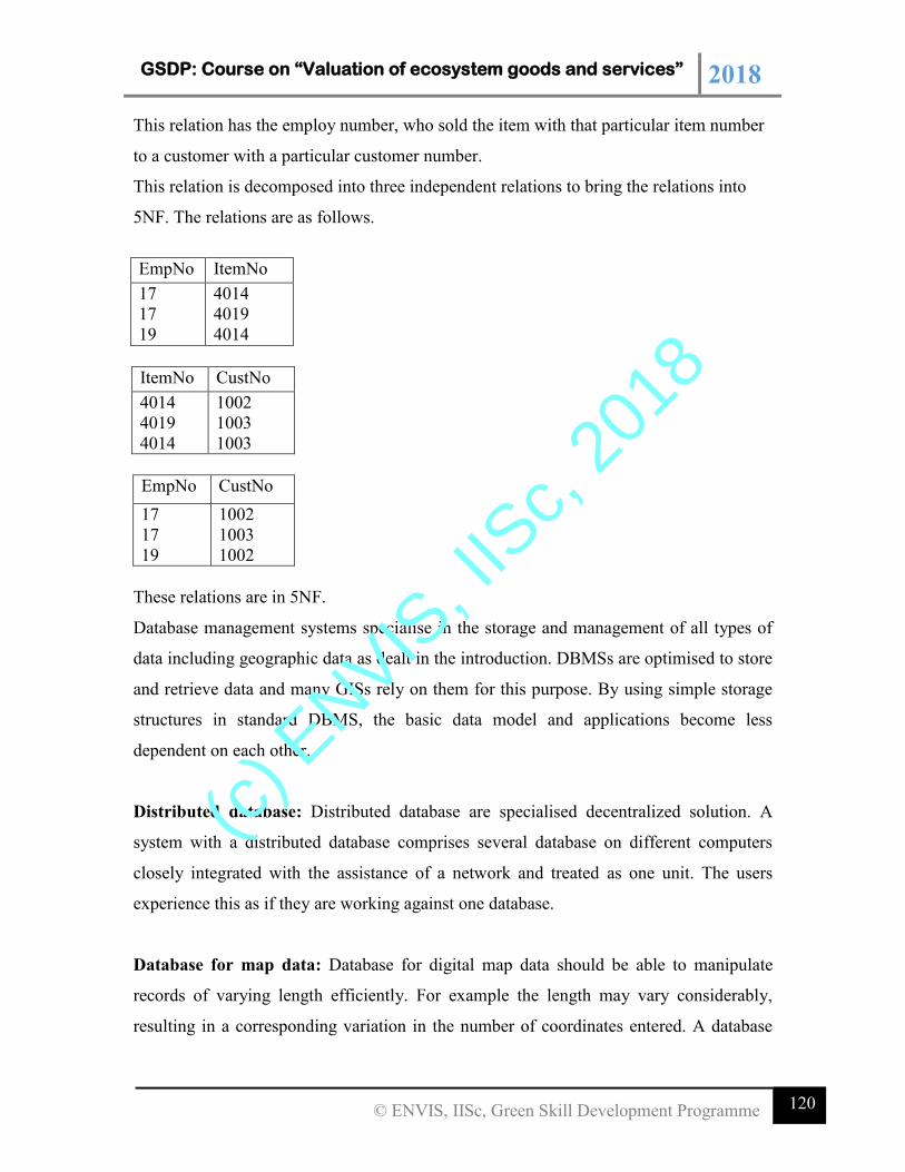
GSDP: Course on “Valuation of ecosystem goods and services” 2018
120 © ENVIS, IISc, Green Skill Development Programme
This relation has the employ number, who sold the item with that particular item number
to a customer with a particular customer number.
This relation is decomposed into three independent relations to bring the relations into
5NF. The relations are as follows.
EmpNo ItemNo
17
17
19
4014
4019
4014
ItemNo CustNo
4014
4019
4014
1002
1003
1003
EmpNo CustNo
17
17
19
1002
1003
1002
These relations are in 5NF.
Database management systems specialise in the storage and management of all types of
data including geographic data as dealt in the introduction. DBMSs are optimised to store
and retrieve data and many GISs rely on them for this purpose. By using simple storage
structures in standard DBMS, the basic data model and applications become less
dependent on each other.
Distributed database: Distributed database are specialised decentralized solution. A
system with a distributed database comprises several database on different computers
closely integrated with the assistance of a network and treated as one unit. The users
experience this as if they are working against one database.
Database for map data: Database for digital map data should be able to manipulate
records of varying length efficiently. For example the length may vary considerably,
resulting in a corresponding variation in the number of coordinates entered. A database
(c) E
NVIS, I
ISc,
2018
GSDP: Course on “Valuation of ecosystem goods and services” 2018
121 © ENVIS, IISc, Green Skill Development Programme
system should reflect geographic reality by such means as requiring that data on object of
the same type, such as the lines forming a property boundary, be stored in the close
proximity in the database, to speed up the response.
Partitioning and Indexing: We have ascertained that spaghetti data require a long
search time since the data are stored in a relatively casual and unconnected sequence in
this file. The time used to search for and retrieve topological data is also governed by the
way in which the data are structured for storage. A rational data structure will reduce the
storage volume. Special techniques have therefore been developed for dividing and
structuring data.
Generally, map data are stored in map sheets or other geographical units, but storing map
sheet data in single sequential files lengthens the response time. This has resulted in some
GISs employing indexing to speed up the searching process, and enabling current map
sheets to appear on screen almost immediately. Indexing specifies locations, so map
sheets are divided into sections which are distributed in such a manner as to accelerate
the search. For example, zooming focuses on data in those sections relevant to a selected
area and ignores the remainder of the map sheet.
The use of traditional hashing techniques and trees makes it very difficult to handle
divided areas that overlap. However, routines have been developed that can handle
overlapping data relatively efficiently. These have also been implemented for object-
oriented solutions. In recent years, more powerful and rapid hardware has made it easier
to use simple data structures for storage, but many GISs still use different “smart”
solutions to obtain rapid access to data stored on the disk.
No current database system or structure completely fulfils the needs of database
applications. There are grounds for suspecting that the excessively complex and
voluminous data collections of many GISs may be ascribed to the databases employed. It
goes without saying, then, that further database development is in order. One goal might
be to develop better object-oriented database systems.
(c) E
NVIS, I
ISc,
2018
GSDP: Course on “Valuation of ecosystem goods and services” 2018
122 © ENVIS, IISc, Green Skill Development Programme
Structured Query Language: The simple structures of relational database systems have
permitted the development of standard query languages, one of which is Structured
Query Language (SQL). SQL gives users access to data in relational DBMSs by
describing the data they may wish to see. SQL also allows users to define data in a
database and to manipulate those data. Additional functions that SQL supplies to
relational databases are very useful for many GIS applications.
Relational algebra may be performed using two classes of storage and retrieval
operations. The set operations include union, intersection, difference, and product. The
relational operations include selection (accessing rows), projection (accessing columns),
joining, and dividing. Relational joining links tables and creates a new table from data
retrieved from various tables. The new table need not be stored physically in the
database.
There are six logical operations in SQL:
1. = Equal
2. <> Not Equal
3. < Less than
4. > Greater then
5. Less than or equal
6. Greater than or equal
There are five aggregate functions:
1. The total of all rows, satisfying any conditions, of the given column, where the
given column is numerical
2. The average of the given column
3. The largest figure in the given column
4. The smallest figure in the given column
5. The number of rows satisfying the conditions
(c) E
NVIS, I
ISc,
2018
GSDP: Course on “Valuation of ecosystem goods and services” 2018
123 © ENVIS, IISc, Green Skill Development Programme
Most GIS users have developed application programs with various human—machine
interfaces. SQL is used most frequently in searching, although other query procedures are
also used. Complex GIS functions such as data search within specified rectangles or
circles, creation of buffer zones, and overlay require operations that are not implemented
in standard SQL. However, several suppliers of GIS software have developed special
SQL dialects. This applies in particular to systems that use relational databases for
storage of both geometry and attributes.
Organization of Data Storage Operations
Software systems often organize data to ensure effective use. Such organization may
involve various logical paradigms concerning the grouping of object types and the
divisions of geographical areas. The physical limitations of system file capacities may
also be a practical reason for thematic and geographic divisions. A list of all maps in a
system, organized by location and theme, forms a map library, from which the user can
select the map he or she needs and store it in the workspace of the computer.
Thematic layers: Data in most GIS are organized in layers (levels), much like the
overlays of conventional mapmaking. Similarly, individual data layers are stored in
individual data files. These layers may contain object types intended to be processed
together, such as points in one layer, lines in another, and polygons in a third.
Alternatively, the individual data layers may be organized by theme, perhaps one layer
for topography, another for property boundaries, others for roads or types of land use, and
so on. Furthermore, each layer may contain subsidiary layers in a hierarchy. Thus a layer
for roads might encompass subsidiary layers for national, county, urban, and private
roads.
Collecting logically similar objects can reduce the amount of data required to describe
an individual object. Objects that represent several themes, such as lines that are
simultaneously roads and property or land-use area boundaries, may be collected in one
layer. The line geometry of that layer may be transferred to other layers as needed.
(c) E
NVIS, I
ISc,
2018
GSDP: Course on “Valuation of ecosystem goods and services” 2018
124 © ENVIS, IISc, Green Skill Development Programme
Objects that are updated frequently or from the same source of information may also be
collected in a single layer to facilitate updating work. The cartographic effects of plotting
are frequently dependent on the sequential plotting of layers containing like objects.
The separation of data into layers may seem analogous to the traditional separation of
map information into overlays, and therefore not always a realistic data model of reality.
One of the reasons for this layered storage is that many earlier systems have not been able
to store overlapping polygons in the same layer. Today, however, there are systems that
can handle this problem. These GISs circumvent “map overlay thinking” by being more
object oriented; that is, each object is manipulated as an independent entity with regard to
both its geometry and its attributes.
Partitioning the area: Many GISs have facilities that will divide surfaces to promote
efficient storage, use, and updating of data. Individual surface segments are then stored in
individual files, division by map sheets being the most common. Some GISs support
divisions of data structures into projects, each of which may then be further divided into
subprojects.
The manipulation of data for a larger area often involves combining data for their
constituent segments. This is done either manually by the user or automatically by the
system. As many GISs are seamless (i.e., data need not be regarded as belonging to fixed
map sheets), though stored data may be divided into map sheets, which in turn may be
divided into cells in grids .
Users must select the most suitable elements for storing data, such as the map sheet sizes
and area divisions. Choice is vital for two reasons. First, the organization of data storage
elements can have a considerable influence on the efficiency with which data are been
used. Second, once the storage elements are chosen and data have been stored,
restructuring to other storage elements is extremely complicated.
(c) E
NVIS, I
ISc,
2018
GSDP: Course on “Valuation of ecosystem goods and services” 2018
125 © ENVIS, IISc, Green Skill Development Programme
Editing Attribute Data: Like digital map data, attribute data must be edited and
corrected. These operations include error correction, updating, and amending. The editing
tasks may be carried out by using standard editing tools, such as those available in word
processing, or specific GIS commands. Some GISs use SQL (Structured Query
Language) to manipulate attribute data in relational databases. Specific GIS commands
include commands for changing object thematic codes and switching codes between
objects, as well as for editing thematic codes containing texts.
The guidelines for entering data may change with time, mandating changes in the
codes of older data. Usually, common mathematical signs as +. -, * and / are used for this
purpose. The currencies in which prices in attributes are expressed may be changed [e.g.,
from U.S. dollars ($) to Indian rupees (Rs.)] by entering an exchange rate. Relational and
other databases used to store attribute data usually incorporate effective editing tools.
These permit a variety of operations, including searching for members of a prescribed
class and then editing one by one, or assigning new values to an entire class using a
single command.
(c) E
NVIS, I
ISc,
2018
GSDP: Course on “Valuation of ecosystem goods and services” 2018
126 © ENVIS, IISc, Green Skill Development Programme
Chapter 5: Basic Spatial Analysis
Analysis of Spatial Information
Even though most of the real world can be observed with the naked eye, it is often
difficult to interpret and systematize what is observed. It becomes even more difficult
when the image of that reality is stored in digital form as map data and attribute tables.
To bring out the patterns, connections, and possibly, the causes of variations in the data,
various computer-based techniques are applied to analyse the data. Spatial analysis
techniques are an attempt to imitate what concerns the human brain (i.e., to create an
understandable image of reality). These are the techniques discussed in this and the
following chapter.
Technology can still only help to a limited extent, however. Stating problems and
delineating the approaches to solutions together comprise one of the most difficult steps
in GIS analysing. This has to be solved by the individual user or operator before the
technology can be put into use, based on his or her professional knowledge in the fields
of agriculture, environmental protection, planning, and so on, supplemented with
knowledge of GIS. Analysing data normally comprises two principal phases:
1. Choice of data
2. Analyses of the data chosen
All GISs provide functions for analyses of data chosen and for storing the results of such
analyses. Data may be selected according to
Geographical location
Thematic content
Most GISs permit defining the criteria for selection. These are often based in SQL or
are in menus with provisions for generating SQL queries. Some GISs provide predefined
selection criteria; other systems use a macro language to set up the selection criteria.
(c) E
NVIS, I
ISc,
2018
GSDP: Course on “Valuation of ecosystem goods and services” 2018
127 © ENVIS, IISc, Green Skill Development Programme
Specific systems have predefined menus dedicated to the relevant applications. In most
systems, selection criteria may be stored for subsequent use.
Data may be analysed at various levels:
1. Data in attribute tables are sorted for presentation in reports or for use in other
computer systems.
2. Operations are performed on geometric data, either in search mode or for
computational purposes.
3. Arithmetic, Boolean, and statistical operations are performed in attribute tables.
4. Geometry and attribute tables are used jointly to:
a. Compile new sets of data, based on original and derived attributes
b. Compile new sets of data based on geographical relationships.
Within each of these levels, the operations used may be logical, arithmetic, geometric,
statistical, or a combination of two or more of these four types. Operations may be
performed on individual points or on areas, and may involve considerations of proximity
or of changes over time. Numerous operations may be performed on line networks. The
more important commands are discussed below. The functions implemented vary from
one GIS to another, and some GISs contain functions not discussed here.
Logic Operations: Logical searches in databases normally employ set algebra or
Boolean algebra. Set algebra uses the three operators equal to, greater than, and less than,
and combinations thereof:
=, >, <, , , <>
These operators are included under SQL.
Practical applications include:
Identifying extrema, such as finding attribute minima or maxima within various
polygons and, as a result, delineating a new thematic layer (new row in the
attribute table)
Selection or isolation, where particular values are selected for subsequent ranking
in a new thematic layer
(c) E
NVIS, I
ISc,
2018
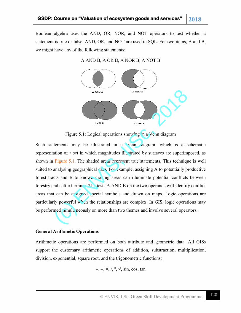
GSDP: Course on “Valuation of ecosystem goods and services” 2018
128 © ENVIS, IISc, Green Skill Development Programme
Boolean algebra uses the AND, OR, NOR, and NOT operators to test whether a
statement is true or false. AND, OR, and NOT are used in SQL. For two items, A and B,
we might have any of the following statements:
A AND B, A OR B, A NOR B, A NOT B
Figure 5.1: Logical operations showing in a Venn diagram
Such statements may be illustrated in a Venn diagram, which is a schematic
representation of a set in which magnitudes illustrated by surfaces are superimposed, as
shown in Figure 5.1. The shaded areas represent true statements. This technique is well
suited to analysing geographical data. For example, assigning A to potentially productive
forest tracts and B to known grazing areas can illuminate potential conflicts between
forestry and cattle farming. The tests A AND B on the two operands will identify conflict
areas that can be assigned special symbols and drawn on maps. Logic operations are
particularly powerful when the relationships are complex. In GIS, logic operations may
be performed simultaneously on more than two themes and involve several operators.
General Arithmetic Operations
Arithmetic operations are performed on both attribute and geometric data. All GISs
support the customary arithmetic operations of addition, substraction, multiplication,
division, exponential, square root, and the trigonometric functions:
, , ×, /, n, , sin, cos, tan
(c) E
NVIS, I
ISc,
2018
GSDP: Course on “Valuation of ecosystem goods and services” 2018
129 © ENVIS, IISc, Green Skill Development Programme
these operators may be used for many purposes, including assigning new thematic codes.
Typical examples include:
Reclassification of soil types, in which areas are to be converted from square
kilometers to hectares by dividing all area figures by 10.
Conversion of distances along roads to driving times, by dividing all distances by a
specified average vehicle speed. The result is a new set of attributes that are useful
in transportation planning.
Arithmetic functions are used in all geometric computations involving coordinates, as in
calculating distances, areas, volumes, and directions.
General Statistical Operations
Statistical operations are performed primarily on attribute data, but may also be effected
on some types of geometric data. Most GISs support a range of statistical operations,
including sum, maxima, minima, average, weighted average, frequency distribution, bi-
directional comparison, standard deviation, multivariate, and others. The computation of
averages requires averaging two or more attribute values and stating the result as a new
attribute. Frequency distributions are used to compile histograms, charts comprising
rectangles whose areas are proportional to relative frequencies and whose widths are
proportional to class intervals. The data used to draw a histogram may also be employed
to plot a curve. Other statistical operations in common use include least-squares
computations of transformation parameters from regression models, with the standard
deviation as an expression of accuracy. Bidirectional comparison involves point-by-point
correlation of two themes to produce a new statistical thematic layer and hence a new
attribute.
Satellite data are usually analysed statistically in dedicated image processing systems,
which are often connected to GIS facilities. Some vector GISs support image processing.
Multivariate operations, such as cluster analyses, are vital in image analyses. These
operations assign new classes to entities on the basis of statistical selection criteria.
Pattern recognition based on statistical models is incorporated in some GISs.
(c) E
NVIS, I
ISc,
2018
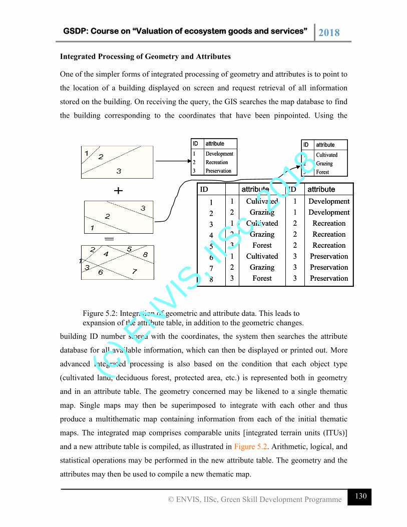
GSDP: Course on “Valuation of ecosystem goods and services” 2018
130 © ENVIS, IISc, Green Skill Development Programme
Integrated Processing of Geometry and Attributes
One of the simpler forms of integrated processing of geometry and attributes is to point to
the location of a building displayed on screen and request retrieval of all information
stored on the building. On receiving the query, the GIS searches the map database to find
the building corresponding to the coordinates that have been pinpointed. Using the
building ID number stored with the coordinates, the system then searches the attribute
database for all available information, which can then be displayed or printed out. More
advanced integrated processing is also based on the condition that each object type
(cultivated land, deciduous forest, protected area, etc.) is represented both in geometry
and in an attribute table. The geometry concerned may be likened to a single thematic
map. Single maps may then be superimposed to integrate with each other and thus
produce a multithematic map containing information from each of the initial thematic
maps. The integrated map comprises comparable units [integrated terrain units (ITUs)]
and a new attribute table is compiled, as illustrated in Figure 5.2. Arithmetic, logical, and
statistical operations may be performed in the new attribute table. The geometry and the
attributes may then be used to compile a new thematic map.
Development
Recreation
Preservation
1
2
3
attributeID
Development
Recreation
Preservation
1
2
3
attributeID
Cultivated
Grazing
Forest
1
2
3
attributeID
Cultivated
Grazing
Forest
1
2
3
attributeID
Development
Development
Recreation
Recreation
Recreation
Preservation
Preservation
Preservation
1
1
2
2
2
3
3
3
Cultivated
Grazing
Cultivated
Grazing
Forest
Cultivated
Grazing
Forest
1
2
1
2
3
1
2
3
1
2
3
4
5
6
7
8
attributeIDattributeID
Development
Development
Recreation
Recreation
Recreation
Preservation
Preservation
Preservation
1
1
2
2
2
3
3
3
Cultivated
Grazing
Cultivated
Grazing
Forest
Cultivated
Grazing
Forest
1
2
1
2
3
1
2
3
1
2
3
4
5
6
7
8
attributeIDattributeID
Figure 5.2: Integration of geometric and attribute data. This leads to
expansion of the attribute table, in addition to the geometric changes.
(c) E
NVIS, I
ISc,
2018
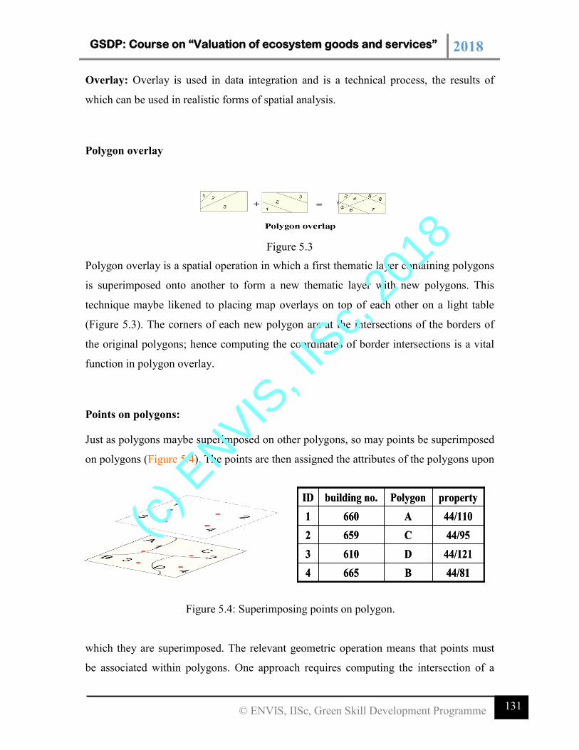
GSDP: Course on “Valuation of ecosystem goods and services” 2018
131 © ENVIS, IISc, Green Skill Development Programme
Overlay: Overlay is used in data integration and is a technical process, the results of
which can be used in realistic forms of spatial analysis.
Polygon overlay
Figure 5.3
Polygon overlay is a spatial operation in which a first thematic layer containing polygons
is superimposed onto another to form a new thematic layer with new polygons. This
technique maybe likened to placing map overlays on top of each other on a light table
(Figure 5.3). The corners of each new polygon are at the intersections of the borders of
the original polygons; hence computing the coordinates of border intersections is a vital
function in polygon overlay.
Points on polygons:
Just as polygons maybe superimposed on other polygons, so may points be superimposed
on polygons (Figure 5.4). The points are then assigned the attributes of the polygons upon
which they are superimposed. The relevant geometric operation means that points must
be associated within polygons. One approach requires computing the intersection of a
44/81B6654
44/121D6103
44/95C 6592
44/110A 6601
propertyPolygonbuilding no.ID
44/81B6654
44/121D6103
44/95C 6592
44/110A 6601
propertyPolygonbuilding no.ID
Figure 5.4: Superimposing points on polygon.
(c) E
NVIS, I
ISc,
2018
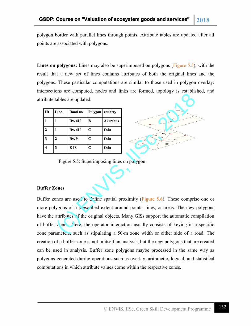
GSDP: Course on “Valuation of ecosystem goods and services” 2018
132 © ENVIS, IISc, Green Skill Development Programme
polygon border with parallel lines through points. Attribute tables are updated after all
points are associated with polygons.
Lines on polygons: Lines may also be superimposed on polygons (Figure 5.5), with the
result that a new set of lines contains attributes of both the original lines and the
polygons. These particular computations are similar to those used in polygon overlay:
intersections are computed, nodes and links are formed, topology is established, and
attribute tables are updated.
Buffer Zones
Buffer zones are used to define spatial proximity (Figure 5.6). These comprise one or
more polygons of a prescribed extent around points, lines, or areas. The new polygons
have the attributes of the original objects. Many GISs support the automatic compilation
of buffer zones. Here, the operator interaction usually consists of keying in a specific
zone parameters, such as stipulating a 50-m zone width or either side of a road. The
creation of a buffer zone is not in itself an analysis, but the new polygons that are created
can be used in analysis. Buffer zone polygons maybe processed in the same way as
polygons generated during operations such as overlay, arithmetic, logical, and statistical
computations in which attribute values come within the respective zones.
Oslo C E 1834
Oslo C Rv. 923
OsloC Rv. 41012
Akershus BRv. 41011
countryPolygon Road noLine ID
Oslo C E 1834
Oslo C Rv. 923
OsloC Rv. 41012
Akershus BRv. 41011
countryPolygon Road noLine ID
Figure 5.5: Superimposing lines on polygon.
(c) E
NVIS, I
ISc,
2018
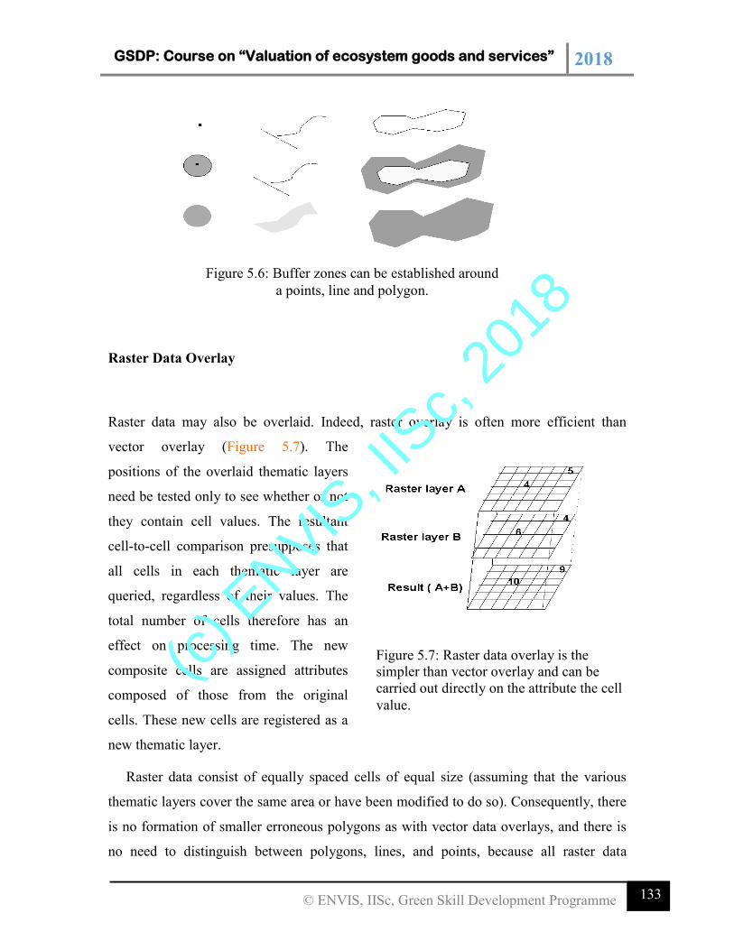
GSDP: Course on “Valuation of ecosystem goods and services” 2018
133 © ENVIS, IISc, Green Skill Development Programme
Raster Data Overlay
Raster data may also be overlaid. Indeed, raster overlay is often more efficient than
vector overlay (Figure 5.7). The
positions of the overlaid thematic layers
need be tested only to see whether or not
they contain cell values. The resultant
cell-to-cell comparison presupposes that
all cells in each thematic layer are
queried, regardless of their values. The
total number of cells therefore has an
effect on processing time. The new
composite cells are assigned attributes
composed of those from the original
cells. These new cells are registered as a
new thematic layer.
Raster data consist of equally spaced cells of equal size (assuming that the various
thematic layers cover the same area or have been modified to do so). Consequently, there
is no formation of smaller erroneous polygons as with vector data overlays, and there is
no need to distinguish between polygons, lines, and points, because all raster data
Figure 5.7: Raster data overlay is the
simpler than vector overlay and can be
carried out directly on the attribute the cell
value.
Figure 5.6: Buffer zones can be established around
a points, line and polygon.
(c) E
NVIS, I
ISc,
2018
GSDP: Course on “Valuation of ecosystem goods and services” 2018
134 © ENVIS, IISc, Green Skill Development Programme
comprise cells. In raster data, attributes are not usually listed in tables as in vector data,
but are represented by thematic layers. Therefore, arithmetic operations and some logical
and statistical operations may be performed directly during the overlay process; two
thematic layers may be combined, subtracted, multiplied, and so on. If for example, an
attribute of volume in liters is to be modified to decilitres, the thematic layer of volumes
merely needs to be multiplied by 10 in each cell of an ancillary thematic layer.
The arithmetic operations on two thematic layers, A and B, produce a new thematic
layer, C, through the operations
C=A + B, C=A –B, C=A/B, C=A x B
Typical logical operations might be
If A> 100, C =10; otherwise C= 0
Or
C= max. (or min.) of A nad B
Some GISs support logical operations in the resultant Clayer but not directly in the
original A and B layers.
As raster overlay is far more efficient than vector overlay, many GISs support functions
for manipulating both raster and vector data. Vector data may be converted to raster data
in order that overlaying can be performed, and results can then be converted back to
vector form.
Procedures in integrated Data analysis:
Integrated data analysis follows fixed procedures:
1.Starting the problem.
2.Adapt the data for geometric operation.
3.Perform the geometric operation.
4.Adapt attributes for the analysis.
(c) E
NVIS, I
ISc,
2018
GSDP: Course on “Valuation of ecosystem goods and services” 2018
135 © ENVIS, IISc, Green Skill Development Programme
5.Perform the analysis.
6.Evaluate the results.
7.Redefine and instigate new analysis if needed.
Stating the problem: It involves defining the problem, and the criteria to be used in the
analysis.
Adapting the data for geometric operations: Data available from a database must be
modified before they can be used for geometric operations.
Performing the geometric operations: Geometric operations, employed to sort out the
objects to be analysed include specification of the buffer zones, overlaying, search and
retrieval, joining polygons, and other operations.
For each task the geometric operations must be defined on the basis of the analytic
criteria involved.
Adapting attributes for analysis: Attribute data must also be processed before analysis.
Attribute table must contain an adequate number of empty rows and columns for new
entries.
Performing attributes analysis: arithmetic, logical and statistical operations are performed
on attribute data associated with the object chosen in geometric phase.
Evaluating the results: The results must be evaluated for their trustworthiness
Redefinitions and instigating new analysis: Unacceptable results must be modified or the
analysis that produced them improved and performed again.
Presenting the final results: Analytical results are best presented in easily read maps and
written reports.
• Selection of a recreational area that can provide a wilderness experience:
Step 1:
a) Remoteness, at a specified distance from the manufactured facilities
b) Reasonable accessibility
(c) E
NVIS, I
ISc,
2018
GSDP: Course on “Valuation of ecosystem goods and services” 2018
136 © ENVIS, IISc, Green Skill Development Programme
c) lakes and streams
d) varied topography
e) A variety of vegetation
Step 2: Map data or attribute data or both be modified by clipping a selected area out of a
map database, modifying the area from hectares to kilometers, etc.
Step3: a) In the location of the recreational area broad buffer zones may be set up around
the roads and other manufacturing facilities.
b) The untouched zones can areas outside these zones may then be overlaid with
vegetation, hydrology and other relevant data.
Step 4: A new attribute labeled “suitable characteristic ” may be complied to hold codes
that indicate the degree of suitability of various combinations of thematic layers.
Step 5: Analysis may be performed to identify all areas outside the buffer zone around
manufactured facilities. another analysis might aim to select areas classified as
moderately hilly, etc.
Step 6: Evaluation is done and if require modifications are made at suitable stage
(c) E
NVIS, I
ISc,
2018
GSDP: Course on “Valuation of ecosystem goods and services” 2018
137 © ENVIS, IISc, Green Skill Development Programme
Bibliography: 1. Peter A Burrough and Rachael A McDonnell, 1998. Principles of Geographic
Information Systems. Oxford University Press, Great Britain.
2. Nicholas Chrisman, 1997. Exploring Geographic Information Systems. John Wiley
and Sons, Inc. NewYork.
3. Tor Bernhardsen, 1999. Geographic Information Systems. John Wiley and Sons, Inc.
New York.
4. 4. Thomas M Lillesand and Ralph W Kiefer, 1994. Remote Sensing and Image
Interpretation. John Wiley and Sons, Inc. New York.
5. Rafael C Gonzalez and Richard E Woods, 1993. Digital Image Processing. Addison-
Wesley Reprint 1998, Gopsons Papers Ltd, India.
6. Paul J Gibson, 2000. Introductory Remote Sensing: Principles and Concepts.
Routledge, London.
7. Paul J Gibson and Claire H Power, 2000. Introductory Remote Sensing: Digital
Image Processing and Applications. Routledge, London.
8. Deekshatulu B L and Rajan Y S, 1984. Remote Sensing. Indian Academy of
Sciences, Bangalore.
9. Gert A Schultz and Edwin T Engman, 2000. Remote Sensing in Hydrology and
Water Management. Springer, Heidelberg.
10. Ramachandra,T.V.; Ahalya,N. (2001 ), Essentials in limnology and geographic
information systems (GIS),Monograph limgis2001 Karnataka Environment Research
Foundation, Bangalore
11. Zhang,Jingxiong; Goodchild,Maihael F. (2002 )Uncertainty in geographical
information,Research monographs in geographic information systems Taylor and
Francis, London
12. Wise,Stephen (2002 ),GIS basics,Taylor & Francis, London
13. Verbyla,David L. (2002 ),Practical GIS analysis,Taylor & Francis, London
14. Korte,George B. (2001 ),GIS book,5th Onward Press Thomson Learning, Australia
15. Sudhira,H.S.; Ramachandra,T.V.; Jagadish,K.S. (2003 ),Urban sprawl pattern
analysis using GIS,CES Technical report no.99 Centre for Ecological Sciences, IISc,
Bangalore
16. Reddy,Anji M. (2001 ), Textbook of remote sensing and geographical information
systems, 2nd BSPublications, Sultan Bazar, Hyderabad
17. Bharath, H.A., Ramachandra, T.V., (2015). Visualization of Urban Growth in
Chennai: spatio-temporal using Geoinformatics, Journal of the Indian Society of
Remote Sensing. 30, pp. 24-38.
18. Ramachandra, T.V., Bharath H. A., Shreejith, K., 2015a. GHG footprint of Major
cities in India, Renewable and Sustainable Energy Reviews. 44, pp.473-495. .
(c) E
NVIS, I
ISc,
2018
GSDP: Course on “Valuation of ecosystem goods and services” 2018
138 © ENVIS, IISc, Green Skill Development Programme
19. Ramachandra, T.V., Bharath, H.A., Sowmyashree M. V., 2015b. Monitoring
urbanization and its implications in a mega city from space: Spatiotemporal patterns
and its indicators, Journal of Environmental Management. 148, pp.67-91. Doi:
10.1016/j.jenvman.2014.02.015 .
20. Ramachandra, T.V., Bharath, H.A., Sowmyashree M. V., 2014. Urban Structure in
Kolkata: Metrics and Modeling through Geo-informatics, Applied Geomatics, 6(4),
229-244. doi: 10.1007/s12518-014-0135-y
21. Ramachandra T.V., Bharath, H.A., Barik, B., 2014. Urbanisation Pattern of Incipient
Mega Region in India, Tema. Journal of Land Use, Mobility and Environment, 7(1),
pp. 83-100.
22. Ramachandra, T.V., Bharath, H. A., Sowmyashree, M. V., 2014. Urban Footprint of
Mumbai - The Commercial Capital of India, Journal of Urban and Regional Analysis,
Vol. 6(1), pp. 71-94.
23. Ramachandra, T.V., Bharath, H. A., Sowmyashree, M. V., 2014. Monitoring spatial
patterns of urban dynamics in Ahmedabad city, textile hub of India, Spatium
International Review. Vol. 31, pp. 85-91. .
24. Ramachandra, T.V., Bharath, S., Bharath, H.A., 2013. Spatio-temporal dynamics
along the terrain gradient of diverse landscape. Journal of Environmental Engineering
and Landscape Management. 22 (1): 50-63.
25. Ramachandra T.V., Subash Chandran M D., Gururaja K V and Sreekantha, 2007.
Cumulative Environmental Impact Assessment, Nova Science Publishers, New York.
26. Ali, Sameer, G. R. Rao, Divakar K. Mesta, Sreekantha, Mukri Vishnu, M. D. Subash
Chandran, K. V. Gururaja, N. V. Joshi, and T. V. Ramachandra. Ecological Status of
Sharavathi Valley Wildlife Sanctuary. Prism Books Pvt Ltd., Bangalore, 2007
27. Ramachandra T.V., 2006. Management of Municipal Solid Waste, Commonwealth
Of Learning, Canada and Indian Institute of Science, Bangalore, Printed by Capital
Publishing Company, New Delhi [Reprinted in 2009 by TERI Press, New Delhi].
28. Ramachandra T.V., 2006.Soil and Groundwater Pollution from Agricultural
Activities, Commonwealth Of Learning, Canada and Indian Institute of Science,
Bangalore, Printed by Capital Publishing Company, New Delhi [Reprinted in 2009
by TERI Press, New Delhi].
29. Vijay Kulkarni and Ramachandra T.V., 2006. Environmental Management,
Commonwealth Of Learning, Canada and Indian Institute of Science, Bangalore,
Printed by Capital Publishing Company, New Delhi [Reprinted in 2009 by TERI
Press, New Delhi].
30. http://ces.iisc.ernet.in/ energy/monograph1/Frontpage.html
31. https://www.researchgate.net/profile/T_V_Ramachandra/contributions
32. https://scholar.google.co.in/citations?user=Woh1fa8AAAAJ&hl=en
33. http://wgbis.ces.iisc.ernet.in/energy/
34. http://wgbis.ces.iisc.ernet.in/biodiversity
(c) E
NVIS, I
ISc,
2018
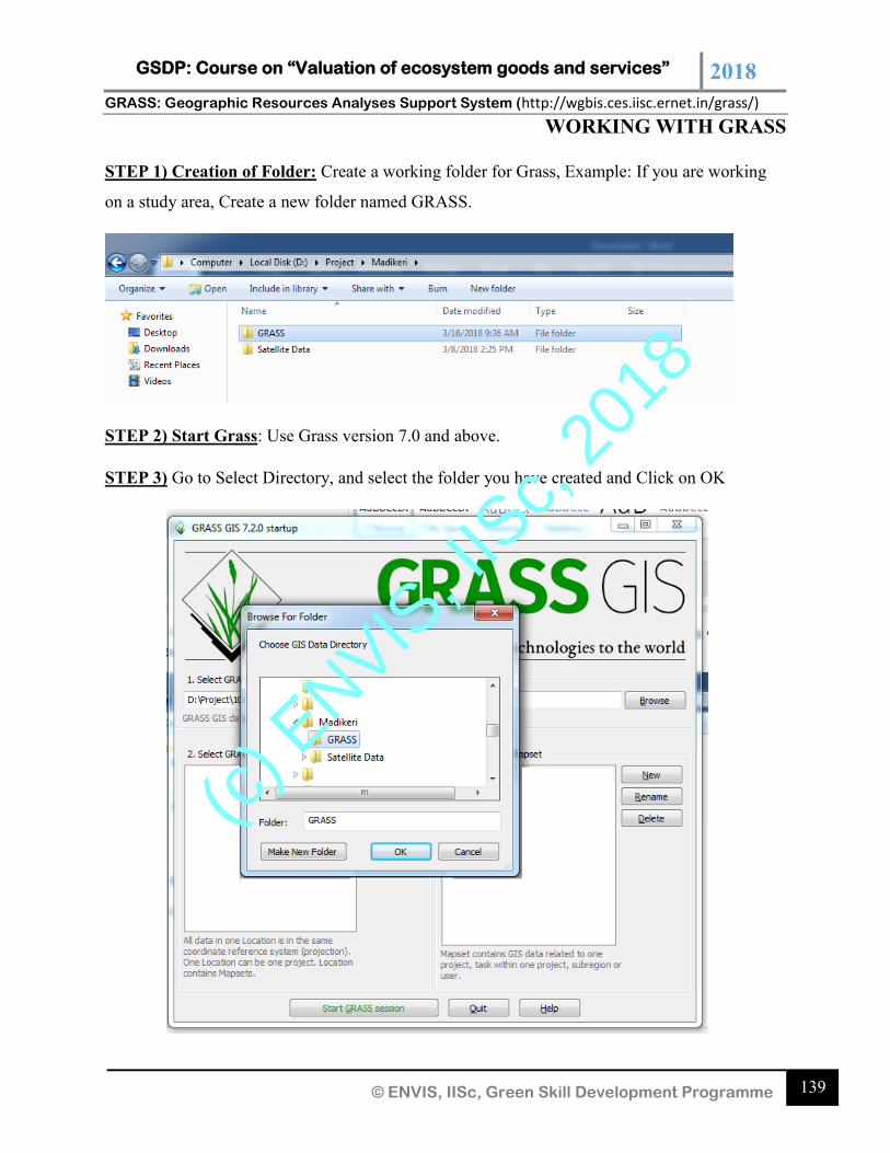
GSDP: Course on “Valuation of ecosystem goods and services” 2018 GRASS: Geographic Resources Analyses Support System (http://wgbis.ces.iisc.ernet.in/grass/)
139 © ENVIS, IISc, Green Skill Development Programme
WORKING WITH GRASS
STEP 1) Creation of Folder: Create a working folder for Grass, Example: If you are working
on a study area, Create a new folder named GRASS.
STEP 2) Start Grass: Use Grass version 7.0 and above.
STEP 3) Go to Select Directory, and select the folder you have created and Click on OK
(c) E
NVIS, I
ISc,
2018
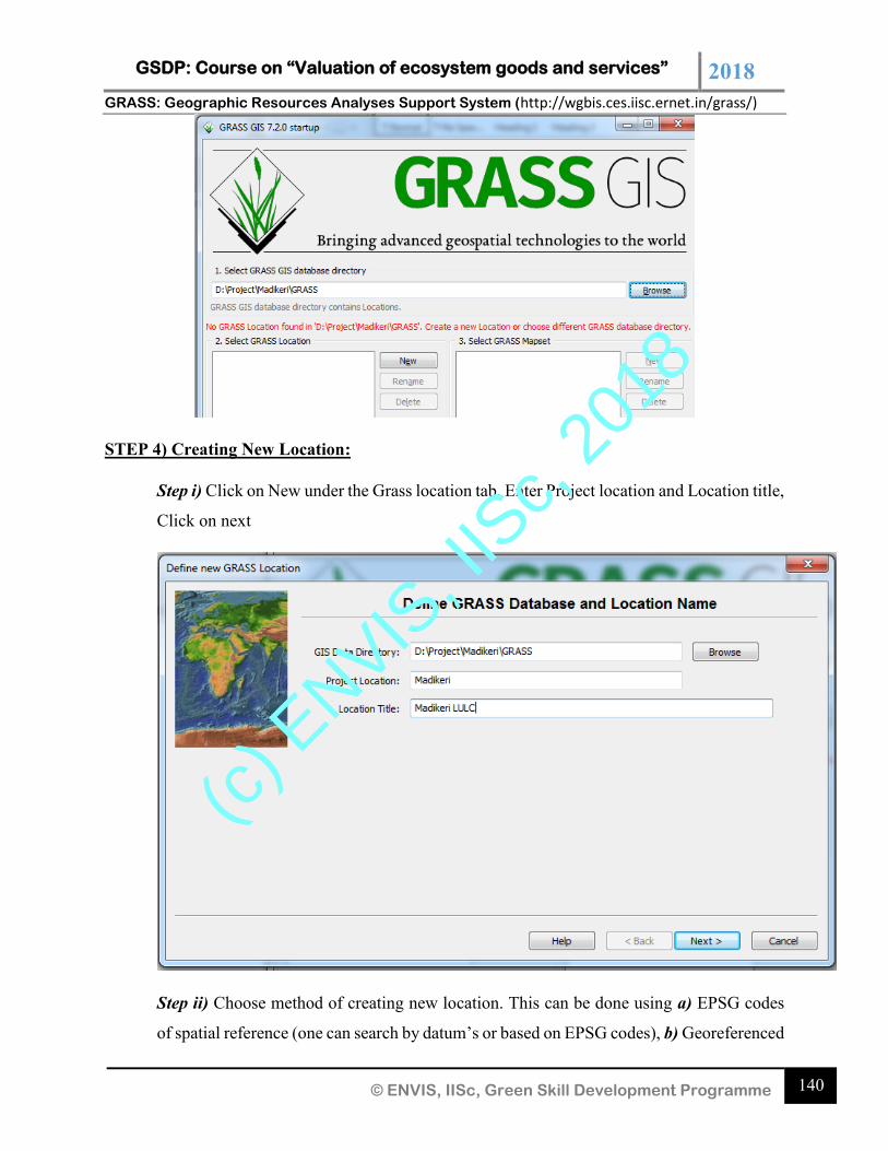
GSDP: Course on “Valuation of ecosystem goods and services” 2018 GRASS: Geographic Resources Analyses Support System (http://wgbis.ces.iisc.ernet.in/grass/)
140 © ENVIS, IISc, Green Skill Development Programme
STEP 4) Creating New Location:
Step i) Click on New under the Grass location tab, Enter Project location and Location title,
Click on next
Step ii) Choose method of creating new location. This can be done using a) EPSG codes
of spatial reference (one can search by datum’s or based on EPSG codes), b) Georeferenced
(c) E
NVIS, I
ISc,
2018
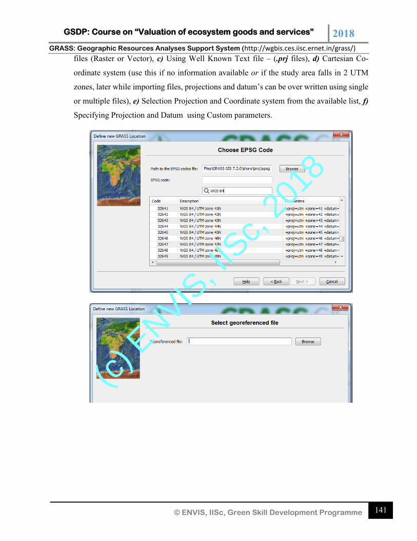
GSDP: Course on “Valuation of ecosystem goods and services” 2018 GRASS: Geographic Resources Analyses Support System (http://wgbis.ces.iisc.ernet.in/grass/)
141 © ENVIS, IISc, Green Skill Development Programme
files (Raster or Vector), c) Using Well Known Text file – (.prj files), d) Cartesian Co-
ordinate system (use this if no information available or if the study area falls in 2 UTM
zones, later while importing files, projections and datum’s can be over written using single
or multiple files), e) Selection Projection and Coordinate system from the available list, f)
Specifying Projection and Datum using Custom parameters.
(c) E
NVIS, I
ISc,
2018
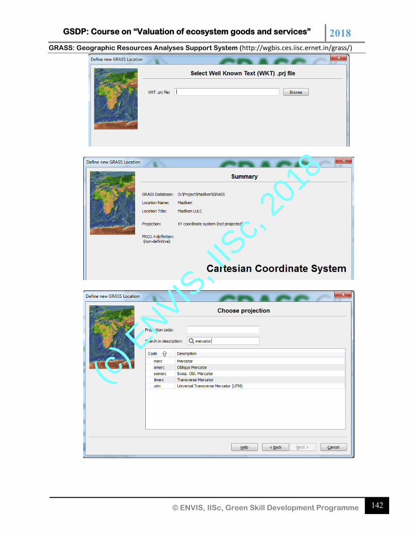
GSDP: Course on “Valuation of ecosystem goods and services” 2018 GRASS: Geographic Resources Analyses Support System (http://wgbis.ces.iisc.ernet.in/grass/)
142 © ENVIS, IISc, Green Skill Development Programme
(c) E
NVIS, I
ISc,
2018
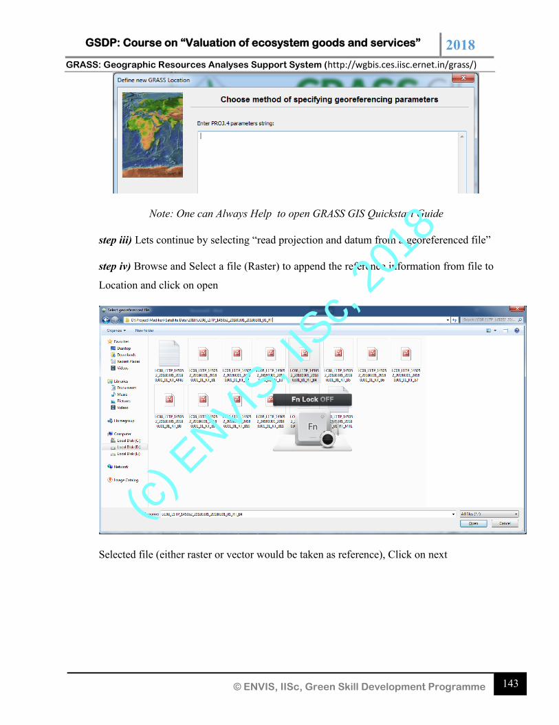
GSDP: Course on “Valuation of ecosystem goods and services” 2018 GRASS: Geographic Resources Analyses Support System (http://wgbis.ces.iisc.ernet.in/grass/)
143 © ENVIS, IISc, Green Skill Development Programme
Note: One can Always Help to open GRASS GIS Quickstart Guide
step iii) Lets continue by selecting “read projection and datum from a georeferenced file”
step iv) Browse and Select a file (Raster) to append the reference information from file to
Location and click on open
Selected file (either raster or vector would be taken as reference), Click on next
(c) E
NVIS, I
ISc,
2018
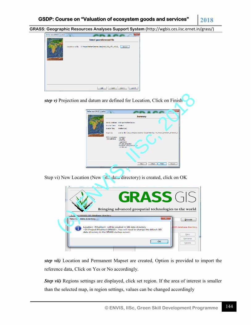
GSDP: Course on “Valuation of ecosystem goods and services” 2018 GRASS: Geographic Resources Analyses Support System (http://wgbis.ces.iisc.ernet.in/grass/)
144 © ENVIS, IISc, Green Skill Development Programme
step v) Projection and datum are defined for Location, Click on Finish
Step vi) New Location (New GIS data directory) is created, click on OK
step vii) Location and Permanent Mapset are created, Option is provided to import the
reference data, Click on Yes or No accordingly.
Step vii) Regions settings are displayed, click set region. If the area of interest is smaller
than the selected map, in region settings, values can be changed accordingly
(c) E
NVIS, I
ISc,
2018
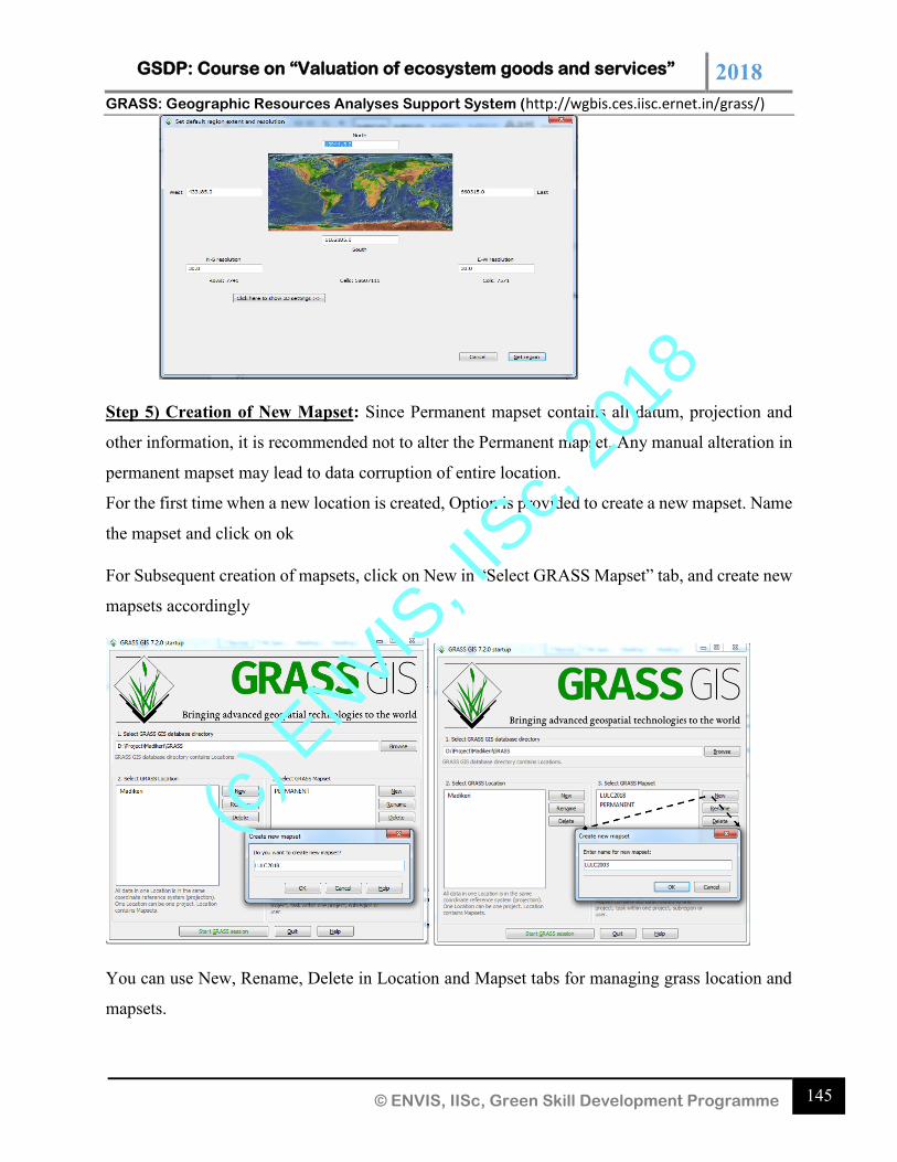
GSDP: Course on “Valuation of ecosystem goods and services” 2018 GRASS: Geographic Resources Analyses Support System (http://wgbis.ces.iisc.ernet.in/grass/)
145 © ENVIS, IISc, Green Skill Development Programme
Step 5) Creation of New Mapset: Since Permanent mapset contains all datum, projection and
other information, it is recommended not to alter the Permanent mapset. Any manual alteration in
permanent mapset may lead to data corruption of entire location.
For the first time when a new location is created, Option is provided to create a new mapset. Name
the mapset and click on ok
For Subsequent creation of mapsets, click on New in “Select GRASS Mapset” tab, and create new
mapsets accordingly
You can use New, Rename, Delete in Location and Mapset tabs for managing grass location and
mapsets.
(c) E
NVIS, I
ISc,
2018
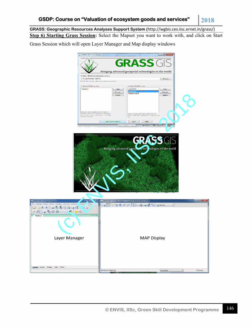
GSDP: Course on “Valuation of ecosystem goods and services” 2018 GRASS: Geographic Resources Analyses Support System (http://wgbis.ces.iisc.ernet.in/grass/)
146 © ENVIS, IISc, Green Skill Development Programme
Step 6) Starting Grass Session: Select the Mapset you want to work with, and click on Start
Grass Session which will open Layer Manager and Map display windows
(c) E
NVIS, I
ISc,
2018
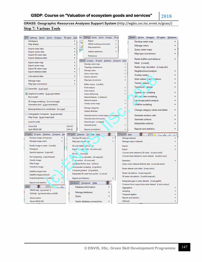
GSDP: Course on “Valuation of ecosystem goods and services” 2018 GRASS: Geographic Resources Analyses Support System (http://wgbis.ces.iisc.ernet.in/grass/)
147 © ENVIS, IISc, Green Skill Development Programme
Step 7: Various Tools
(c) E
NVIS, I
ISc,
2018
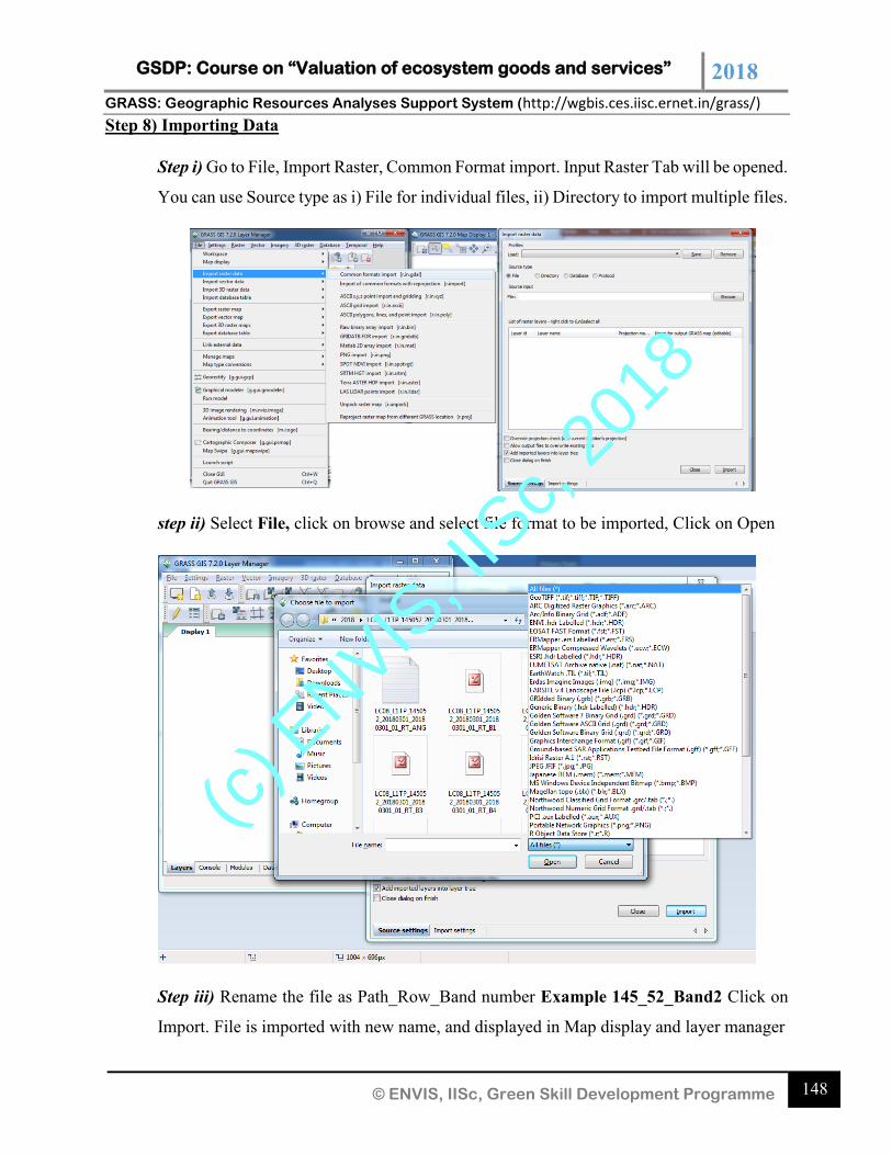
GSDP: Course on “Valuation of ecosystem goods and services” 2018 GRASS: Geographic Resources Analyses Support System (http://wgbis.ces.iisc.ernet.in/grass/)
148 © ENVIS, IISc, Green Skill Development Programme
Step 8) Importing Data
Step i) Go to File, Import Raster, Common Format import. Input Raster Tab will be opened.
You can use Source type as i) File for individual files, ii) Directory to import multiple files.
step ii) Select File, click on browse and select file format to be imported, Click on Open
Step iii) Rename the file as Path_Row_Band number Example 145_52_Band2 Click on
Import. File is imported with new name, and displayed in Map display and layer manager
(c) E
NVIS, I
ISc,
2018
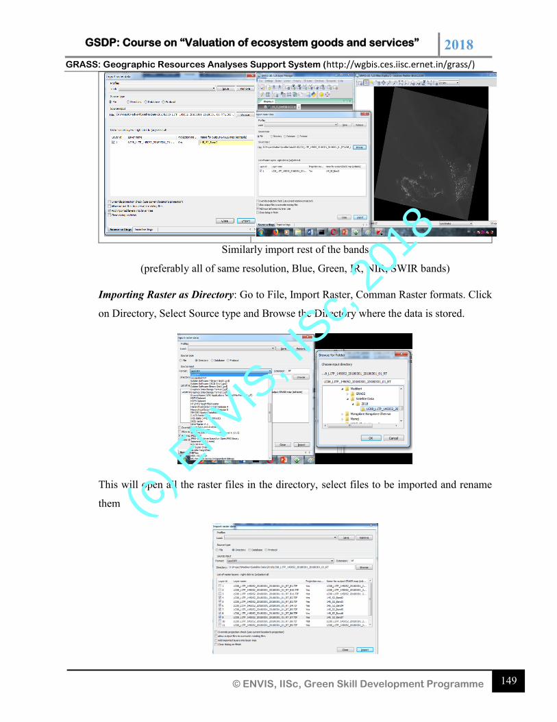
GSDP: Course on “Valuation of ecosystem goods and services” 2018 GRASS: Geographic Resources Analyses Support System (http://wgbis.ces.iisc.ernet.in/grass/)
149 © ENVIS, IISc, Green Skill Development Programme
Similarly import rest of the bands
(preferably all of same resolution, Blue, Green, IR, NIR, SWIR bands)
Importing Raster as Directory: Go to File, Import Raster, Comman Raster formats. Click
on Directory, Select Source type and Browse the Directory where the data is stored.
This will open all the raster files in the directory, select files to be imported and rename
them
(c) E
NVIS, I
ISc,
2018
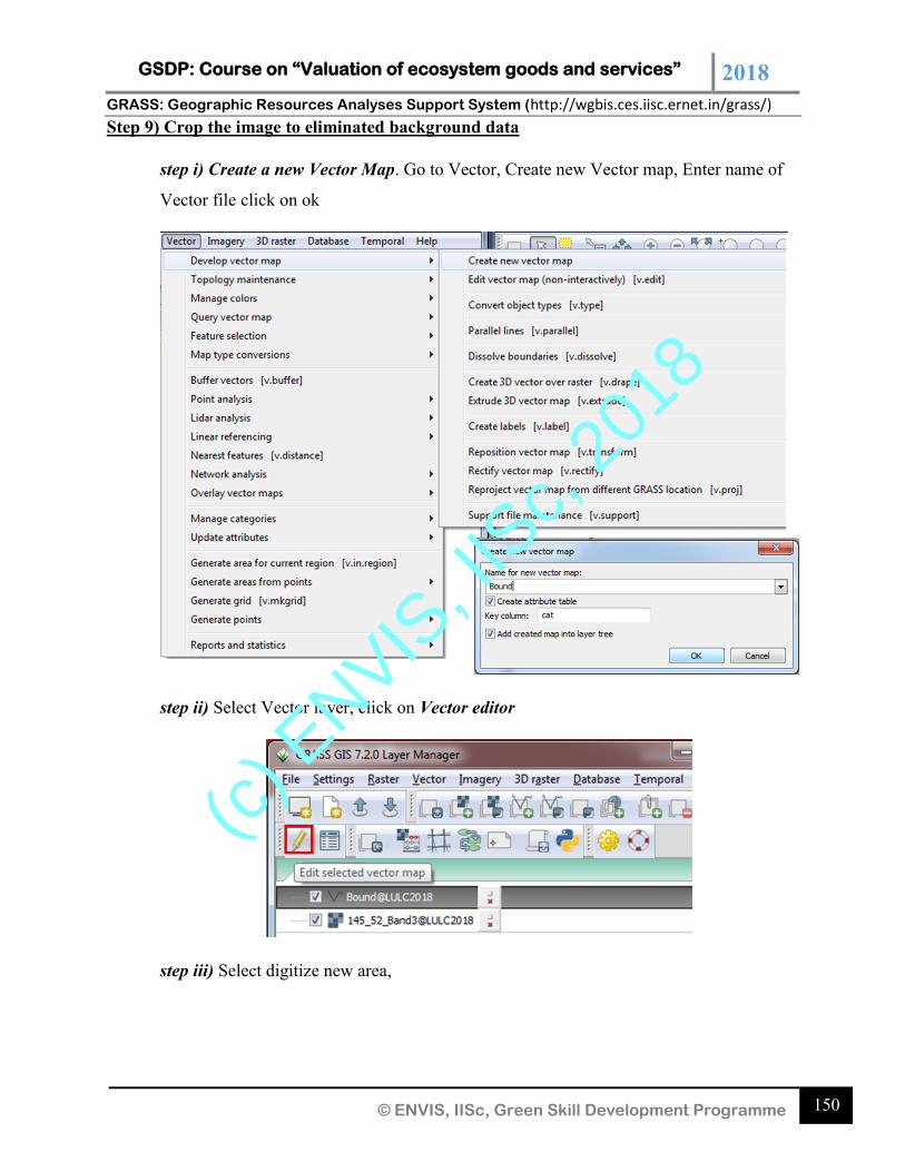
GSDP: Course on “Valuation of ecosystem goods and services” 2018 GRASS: Geographic Resources Analyses Support System (http://wgbis.ces.iisc.ernet.in/grass/)
150 © ENVIS, IISc, Green Skill Development Programme
Step 9) Crop the image to eliminated background data
step i) Create a new Vector Map. Go to Vector, Create new Vector map, Enter name of
Vector file click on ok
step ii) Select Vector layer, click on Vector editor
step iii) Select digitize new area,
(c) E
NVIS, I
ISc,
2018
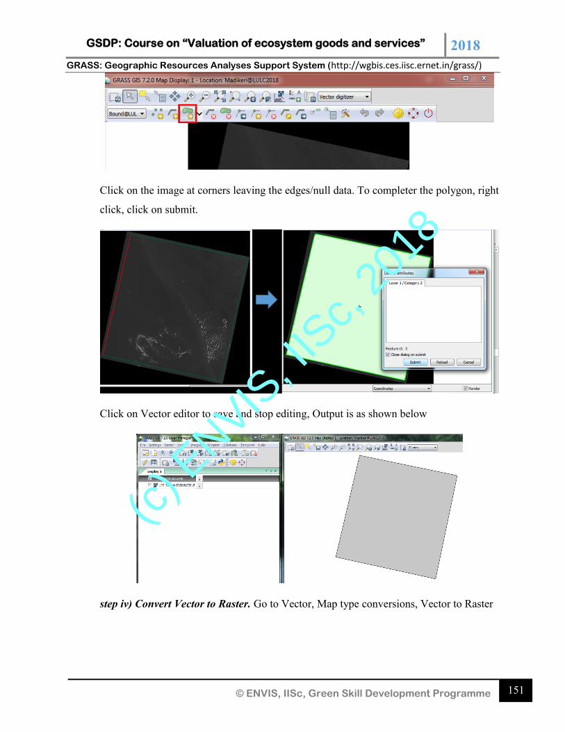
GSDP: Course on “Valuation of ecosystem goods and services” 2018 GRASS: Geographic Resources Analyses Support System (http://wgbis.ces.iisc.ernet.in/grass/)
151 © ENVIS, IISc, Green Skill Development Programme
Click on the image at corners leaving the edges/null data. To completer the polygon, right
click, click on submit.
Click on Vector editor to save and stop editing, Output is as shown below
step iv) Convert Vector to Raster. Go to Vector, Map type conversions, Vector to Raster
(c) E
NVIS, I
ISc,
2018
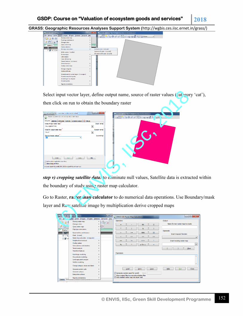
GSDP: Course on “Valuation of ecosystem goods and services” 2018 GRASS: Geographic Resources Analyses Support System (http://wgbis.ces.iisc.ernet.in/grass/)
152 © ENVIS, IISc, Green Skill Development Programme
Select input vector layer, define output name, source of raster values (category ‘cat’),
then click on run to obtain the boundary raster
step v) cropping satellite data: to eliminate null values, Satellite data is extracted within
the boundary of study using raster map calculator.
Go to Raster, raster map calculator to do numerical data operations. Use Boundary/mask
layer and Raw satellite image by multiplication derive cropped maps
(c) E
NVIS, I
ISc,
2018
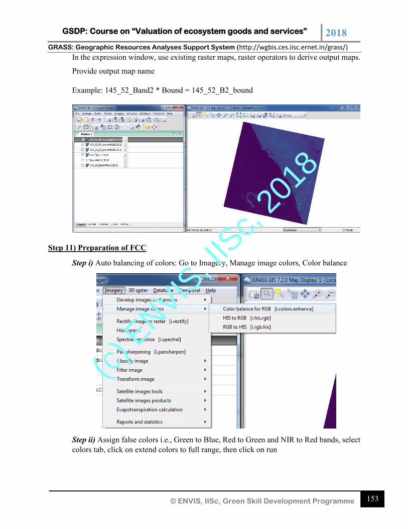
GSDP: Course on “Valuation of ecosystem goods and services” 2018 GRASS: Geographic Resources Analyses Support System (http://wgbis.ces.iisc.ernet.in/grass/)
153 © ENVIS, IISc, Green Skill Development Programme
In the expression window, use existing raster maps, raster operators to derive output maps.
Provide output map name
Example: 145_52_Band2 * Bound = 145_52_B2_bound
Step 11) Preparation of FCC
Step i) Auto balancing of colors: Go to Imagery, Manage image colors, Color balance
Step ii) Assign false colors i.e., Green to Blue, Red to Green and NIR to Red bands, select
colors tab, click on extend colors to full range, then click on run
(c) E
NVIS, I
ISc,
2018
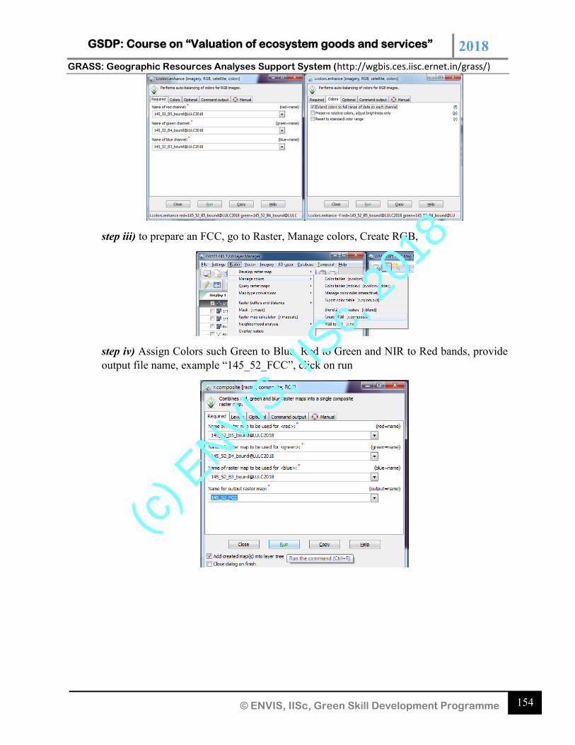
GSDP: Course on “Valuation of ecosystem goods and services” 2018 GRASS: Geographic Resources Analyses Support System (http://wgbis.ces.iisc.ernet.in/grass/)
154 © ENVIS, IISc, Green Skill Development Programme
step iii) to prepare an FCC, go to Raster, Manage colors, Create RGB,
step iv) Assign Colors such Green to Blue, Red to Green and NIR to Red bands, provide
output file name, example “145_52_FCC”, click on run
(c) E
NVIS, I
ISc,
2018
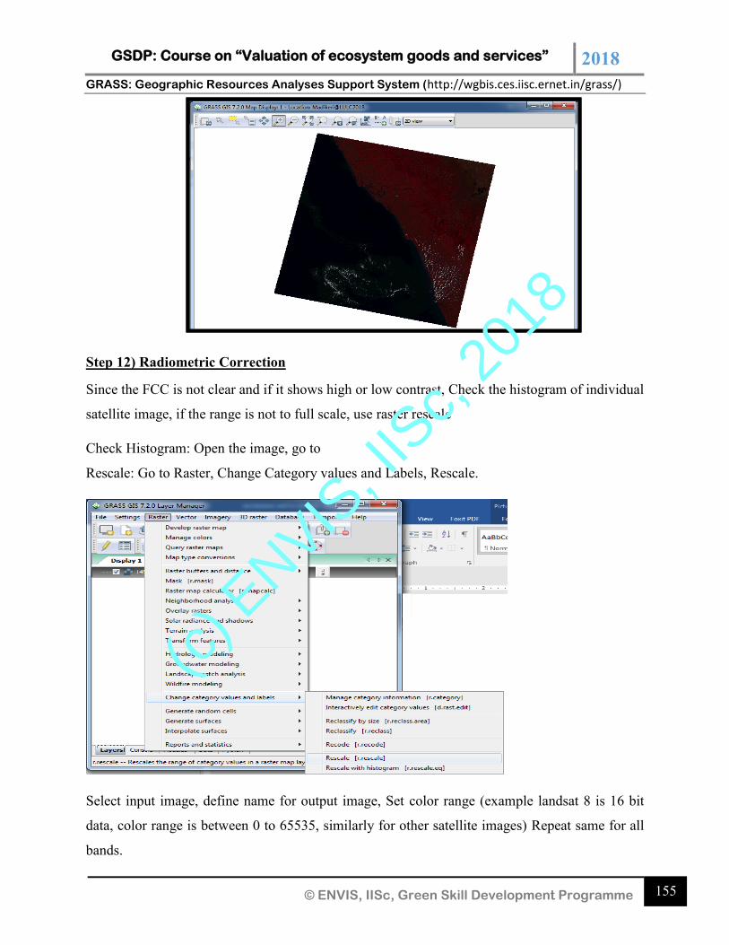
GSDP: Course on “Valuation of ecosystem goods and services” 2018 GRASS: Geographic Resources Analyses Support System (http://wgbis.ces.iisc.ernet.in/grass/)
155 © ENVIS, IISc, Green Skill Development Programme
Step 12) Radiometric Correction
Since the FCC is not clear and if it shows high or low contrast, Check the histogram of individual
satellite image, if the range is not to full scale, use raster rescale
Check Histogram: Open the image, go to
Rescale: Go to Raster, Change Category values and Labels, Rescale.
Select input image, define name for output image, Set color range (example landsat 8 is 16 bit
data, color range is between 0 to 65535, similarly for other satellite images) Repeat same for all
bands.
(c) E
NVIS, I
ISc,
2018
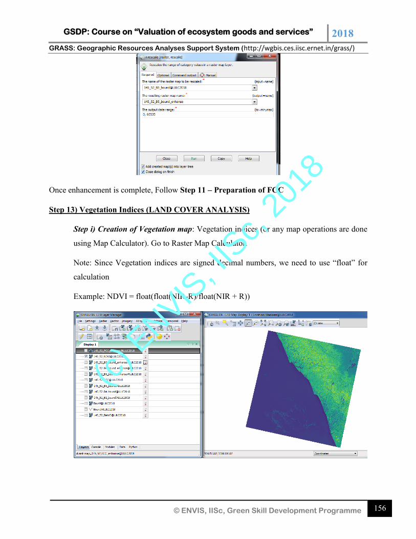
GSDP: Course on “Valuation of ecosystem goods and services” 2018 GRASS: Geographic Resources Analyses Support System (http://wgbis.ces.iisc.ernet.in/grass/)
156 © ENVIS, IISc, Green Skill Development Programme
Once enhancement is complete, Follow Step 11 – Preparation of FCC
Step 13) Vegetation Indices (LAND COVER ANALYSIS)
Step i) Creation of Vegetation map: Vegetation indices (or any map operations are done
using Map Calculator). Go to Raster Map Calculator.
Note: Since Vegetation indices are signed decimal numbers, we need to use “float” for
calculation
Example: NDVI = float(float(NIR-R)/float(NIR + R))
(c) E
NVIS, I
ISc,
2018
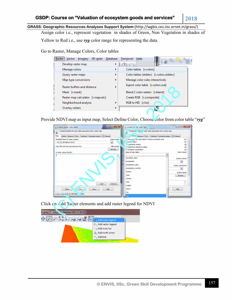
GSDP: Course on “Valuation of ecosystem goods and services” 2018 GRASS: Geographic Resources Analyses Support System (http://wgbis.ces.iisc.ernet.in/grass/)
157 © ENVIS, IISc, Green Skill Development Programme
Assign color i.e., represent vegetation in shades of Green, Non Vegetation in shades of
Yellow to Red i.e., use ryg color range for representing the data.
Go to Raster, Manage Colors, Color tables
Provide NDVI map as input map, Select Define Color, Choose color from color table “ryg”
Click on Add Raster elements and add raster legend for NDVI
(c) E
NVIS, I
ISc,
2018
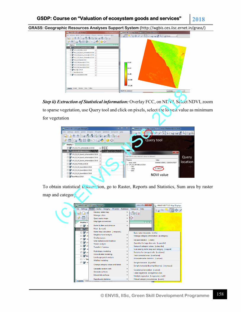
GSDP: Course on “Valuation of ecosystem goods and services” 2018 GRASS: Geographic Resources Analyses Support System (http://wgbis.ces.iisc.ernet.in/grass/)
158 © ENVIS, IISc, Green Skill Development Programme
Step ii) Extraction of Statistical information: Overlay FCC, on NDVI. Select NDVI, zoom
to sparse vegetation, use Query tool and click on pixels, select the lowest value as minimum
for vegetation
To obtain statistical information, go to Raster, Reports and Statistics, Sum area by raster
map and category
(c) E
NVIS, I
ISc,
2018
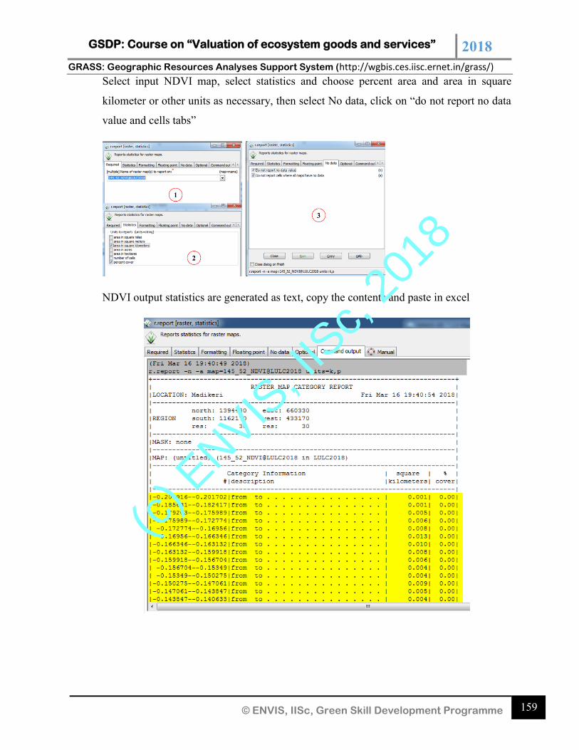
GSDP: Course on “Valuation of ecosystem goods and services” 2018 GRASS: Geographic Resources Analyses Support System (http://wgbis.ces.iisc.ernet.in/grass/)
159 © ENVIS, IISc, Green Skill Development Programme
Select input NDVI map, select statistics and choose percent area and area in square
kilometer or other units as necessary, then select No data, click on “do not report no data
value and cells tabs”
NDVI output statistics are generated as text, copy the contents and paste in excel
(c) E
NVIS, I
ISc,
2018
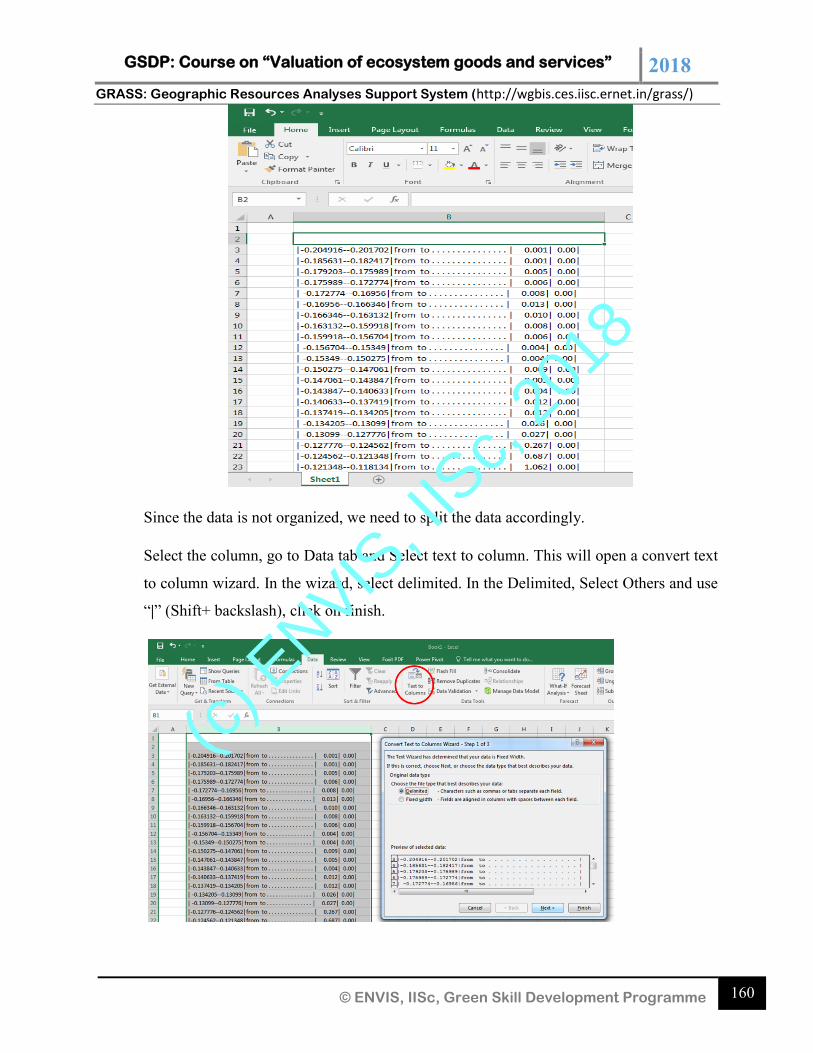
GSDP: Course on “Valuation of ecosystem goods and services” 2018 GRASS: Geographic Resources Analyses Support System (http://wgbis.ces.iisc.ernet.in/grass/)
160 © ENVIS, IISc, Green Skill Development Programme
Since the data is not organized, we need to split the data accordingly.
Select the column, go to Data tab and Select text to column. This will open a convert text
to column wizard. In the wizard, select delimited. In the Delimited, Select Others and use
“|” (Shift+ backslash), click on finish.
(c) E
NVIS, I
ISc,
2018
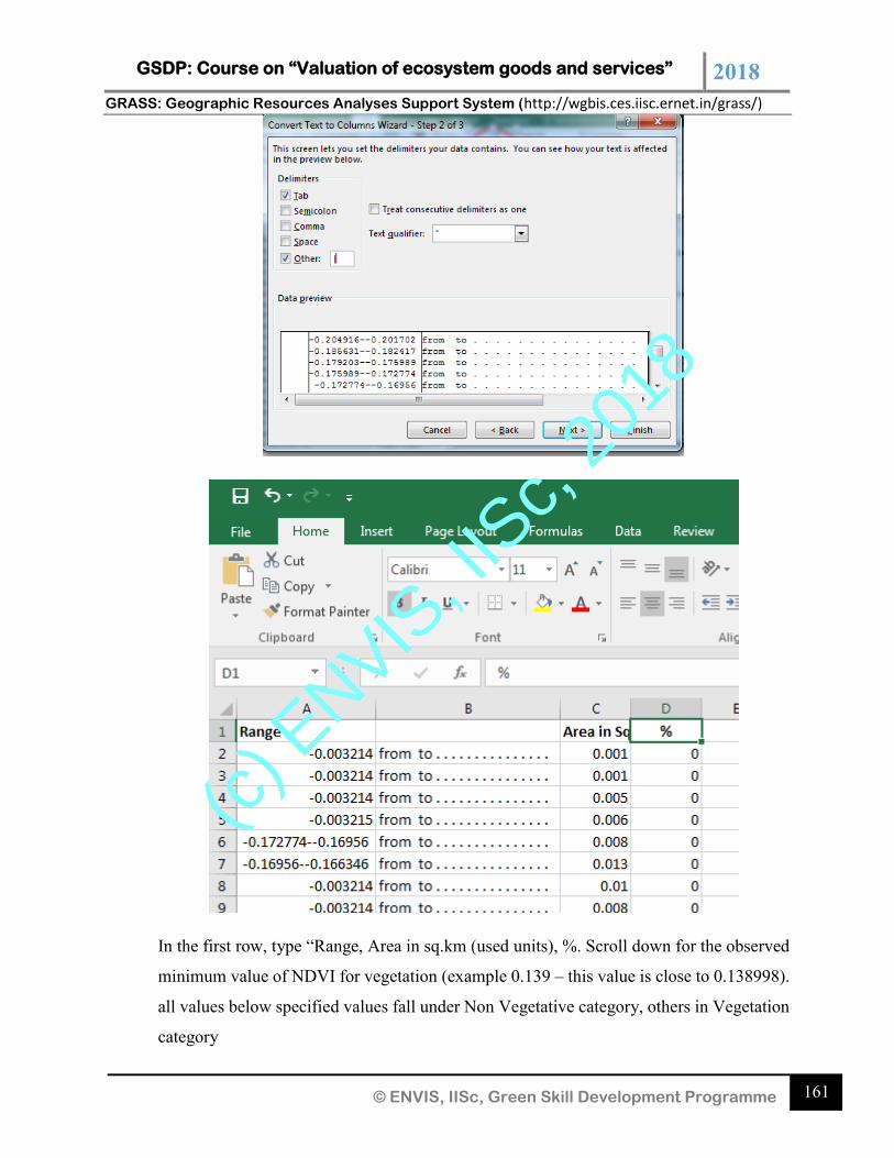
GSDP: Course on “Valuation of ecosystem goods and services” 2018 GRASS: Geographic Resources Analyses Support System (http://wgbis.ces.iisc.ernet.in/grass/)
161 © ENVIS, IISc, Green Skill Development Programme
In the first row, type “Range, Area in sq.km (used units), %. Scroll down for the observed
minimum value of NDVI for vegetation (example 0.139 – this value is close to 0.138998).
all values below specified values fall under Non Vegetative category, others in Vegetation
category
(c) E
NVIS, I
ISc,
2018
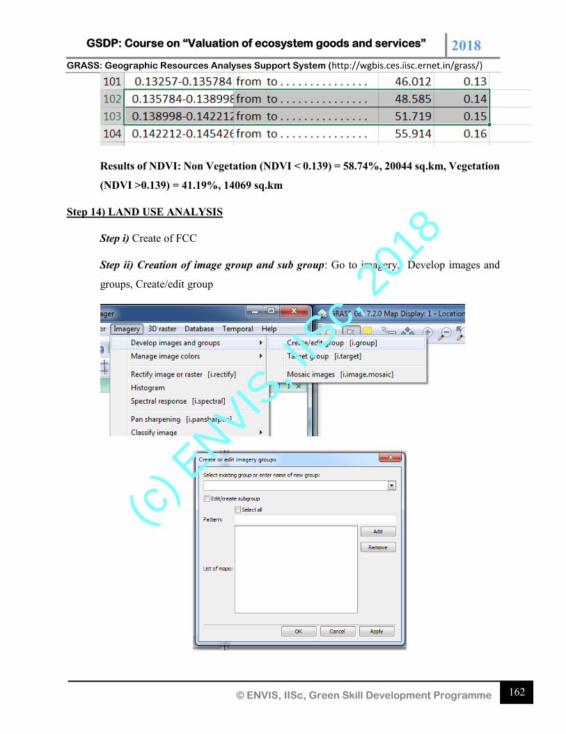
GSDP: Course on “Valuation of ecosystem goods and services” 2018 GRASS: Geographic Resources Analyses Support System (http://wgbis.ces.iisc.ernet.in/grass/)
162 © ENVIS, IISc, Green Skill Development Programme
Results of NDVI: Non Vegetation (NDVI < 0.139) = 58.74%, 20044 sq.km, Vegetation
(NDVI >0.139) = 41.19%, 14069 sq.km
Step 14) LAND USE ANALYSIS
Step i) Create of FCC
Step ii) Creation of image group and sub group: Go to imagery, Develop images and
groups, Create/edit group
(c) E
NVIS, I
ISc,
2018
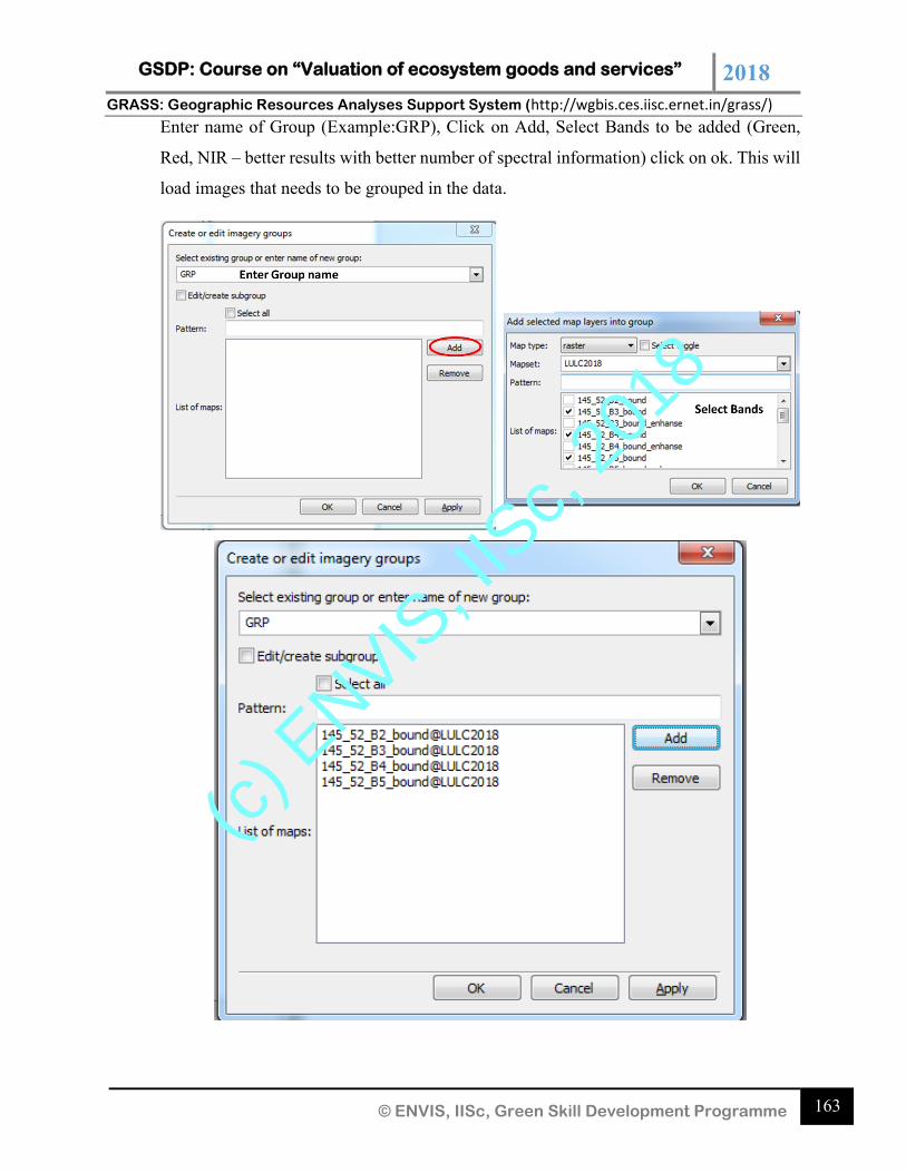
GSDP: Course on “Valuation of ecosystem goods and services” 2018 GRASS: Geographic Resources Analyses Support System (http://wgbis.ces.iisc.ernet.in/grass/)
163 © ENVIS, IISc, Green Skill Development Programme
Enter name of Group (Example:GRP), Click on Add, Select Bands to be added (Green,
Red, NIR – better results with better number of spectral information) click on ok. This will
load images that needs to be grouped in the data.
(c) E
NVIS, I
ISc,
2018
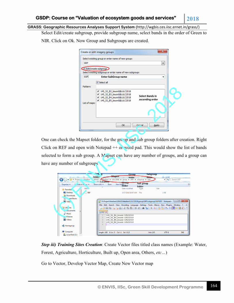
GSDP: Course on “Valuation of ecosystem goods and services” 2018 GRASS: Geographic Resources Analyses Support System (http://wgbis.ces.iisc.ernet.in/grass/)
164 © ENVIS, IISc, Green Skill Development Programme
Select Edit/create subgroup, provide subgroup name, select bands in the order of Green to
NIR. Click on Ok. Now Group and Subgroups are created.
One can check the Mapset folder, for the group and sub group folders after creation. Right
Click on REF and open with Notepad ++ or word pad. This would show the list of bands
selected to form a sub group. A Mapset can have any number of groups, and a group can
have any number of subgroups
Step iii) Training Sites Creation: Create Vector files titled class names (Example: Water,
Forest, Agriculture, Horticulture, Built up, Open area, Others, etc…)
Go to Vector, Develop Vector Map, Create New Vector map
(c) E
NVIS, I
ISc,
2018
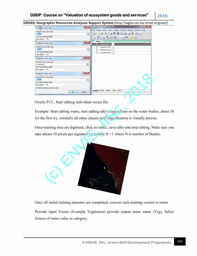
GSDP: Course on “Valuation of ecosystem goods and services” 2018 GRASS: Geographic Resources Analyses Support System (http://wgbis.ces.iisc.ernet.in/grass/)
165 © ENVIS, IISc, Green Skill Development Programme
Overly FCC, Start editing individual vector file
Example: Start editing water, start adding add polygon/lines on the water bodies, about 10
for the first try, similarly all other classes until classification is visually precise.
Once training sites are digitised, click on editor, save edits and stop editing. Make sure you
take atleast 10 pixels per signature (generally N +1 where N is number of Bands)
Once all initial training datasites are completed, convert each training vectors to raster.
Provide input Vector (Example Vegetation) provide output raster name (Veg), Select
Source of raster value as category.
(c) E
NVIS, I
ISc,
2018
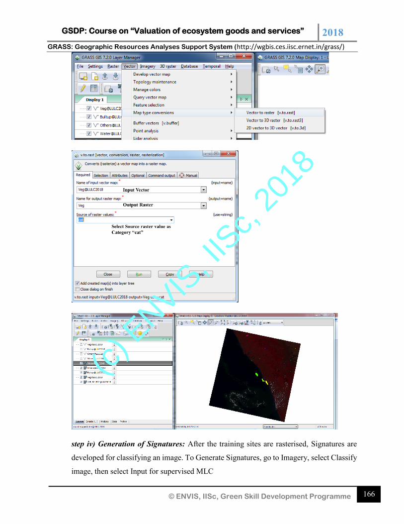
GSDP: Course on “Valuation of ecosystem goods and services” 2018 GRASS: Geographic Resources Analyses Support System (http://wgbis.ces.iisc.ernet.in/grass/)
166 © ENVIS, IISc, Green Skill Development Programme
step iv) Generation of Signatures: After the training sites are rasterised, Signatures are
developed for classifying an image. To Generate Signatures, go to Imagery, select Classify
image, then select Input for supervised MLC
(c) E
NVIS, I
ISc,
2018

GSDP: Course on “Valuation of ecosystem goods and services” 2018 GRASS: Geographic Resources Analyses Support System (http://wgbis.ces.iisc.ernet.in/grass/)
167 © ENVIS, IISc, Green Skill Development Programme
Provide information such as input training file (raster), Group and Subgroup, Output
signature name. Signatures are generated for each land use category separately.
After creating all signatures, go to the signature folder inside the subgroup folder created
in the earlier steps.
(c) E
NVIS, I
ISc,
2018
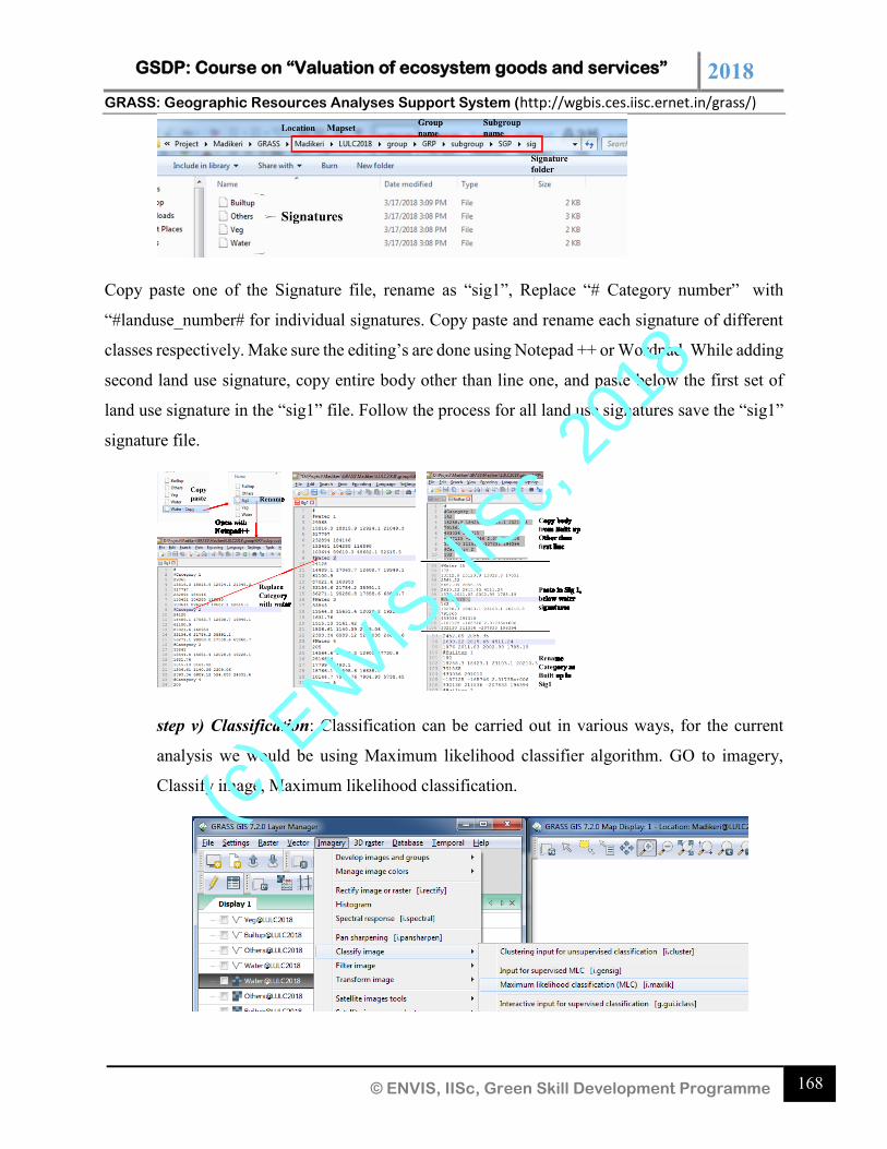
GSDP: Course on “Valuation of ecosystem goods and services” 2018 GRASS: Geographic Resources Analyses Support System (http://wgbis.ces.iisc.ernet.in/grass/)
168 © ENVIS, IISc, Green Skill Development Programme
Copy paste one of the Signature file, rename as “sig1”, Replace “# Category number” with
“#landuse_number# for individual signatures. Copy paste and rename each signature of different
classes respectively. Make sure the editing’s are done using Notepad ++ or Wordpad. While adding
second land use signature, copy entire body other than line one, and paste below the first set of
land use signature in the “sig1” file. Follow the process for all land use signatures save the “sig1”
signature file.
step v) Classification: Classification can be carried out in various ways, for the current
analysis we would be using Maximum likelihood classifier algorithm. GO to imagery,
Classify image, Maximum likelihood classification.
(c) E
NVIS, I
ISc,
2018
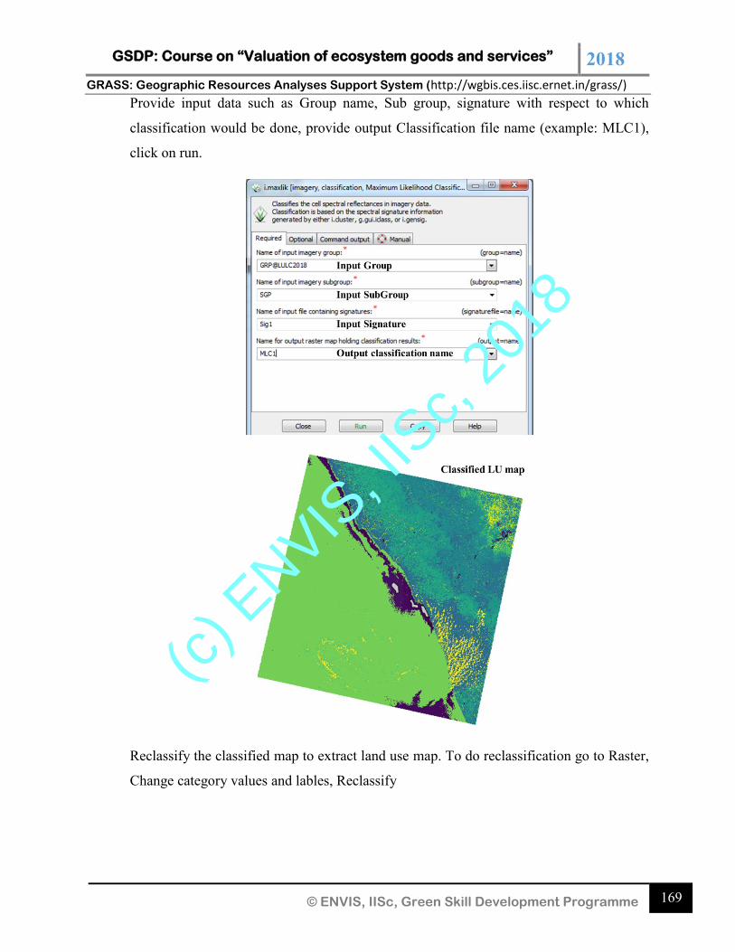
GSDP: Course on “Valuation of ecosystem goods and services” 2018 GRASS: Geographic Resources Analyses Support System (http://wgbis.ces.iisc.ernet.in/grass/)
169 © ENVIS, IISc, Green Skill Development Programme
Provide input data such as Group name, Sub group, signature with respect to which
classification would be done, provide output Classification file name (example: MLC1),
click on run.
Reclassify the classified map to extract land use map. To do reclassification go to Raster,
Change category values and lables, Reclassify
(c) E
NVIS, I
ISc,
2018
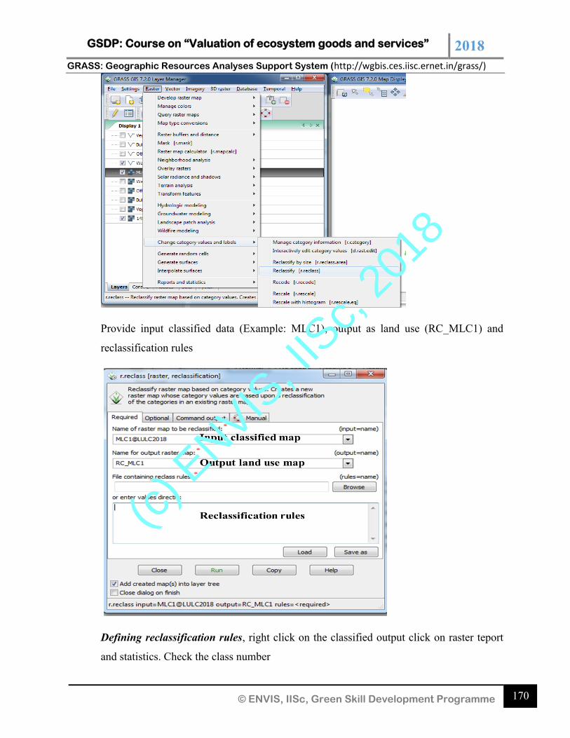
GSDP: Course on “Valuation of ecosystem goods and services” 2018 GRASS: Geographic Resources Analyses Support System (http://wgbis.ces.iisc.ernet.in/grass/)
170 © ENVIS, IISc, Green Skill Development Programme
Provide input classified data (Example: MLC1), output as land use (RC_MLC1) and
reclassification rules
Defining reclassification rules, right click on the classified output click on raster teport
and statistics. Check the class number
(c) E
NVIS, I
ISc,
2018
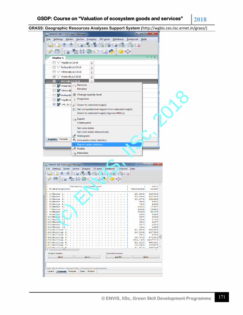
GSDP: Course on “Valuation of ecosystem goods and services” 2018 GRASS: Geographic Resources Analyses Support System (http://wgbis.ces.iisc.ernet.in/grass/)
171 © ENVIS, IISc, Green Skill Development Programme
(c) E
NVIS, I
ISc,
2018
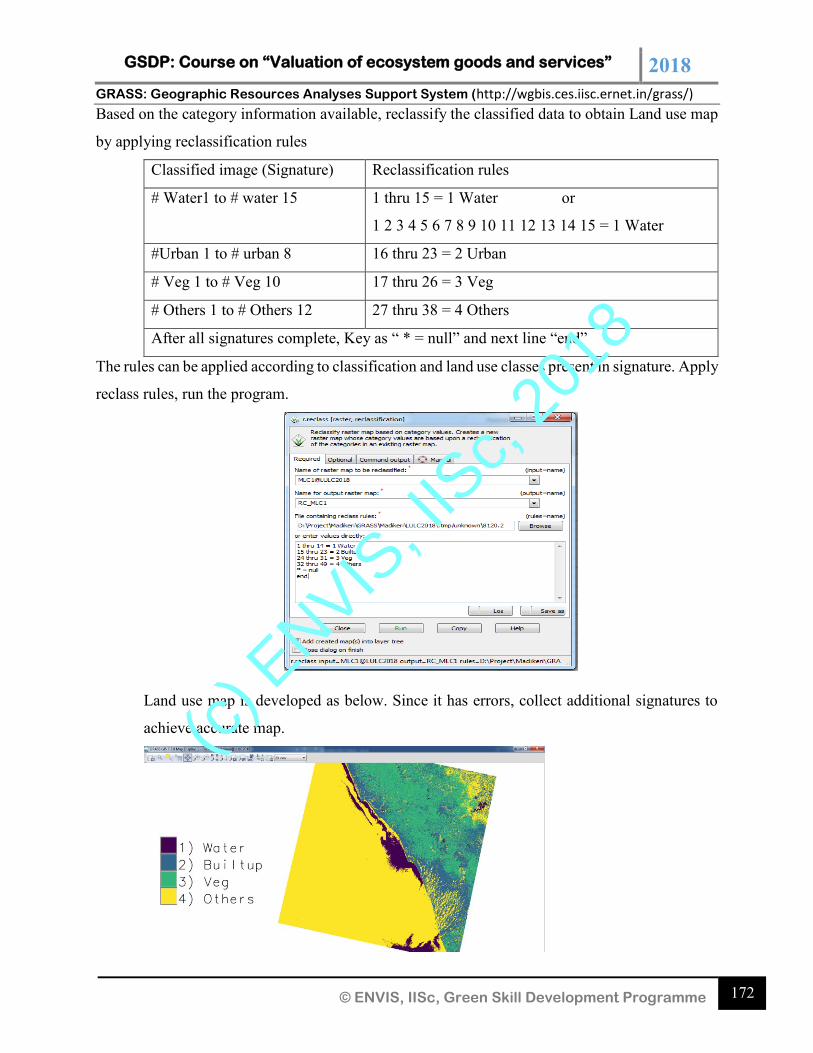
GSDP: Course on “Valuation of ecosystem goods and services” 2018 GRASS: Geographic Resources Analyses Support System (http://wgbis.ces.iisc.ernet.in/grass/)
172 © ENVIS, IISc, Green Skill Development Programme
Based on the category information available, reclassify the classified data to obtain Land use map
by applying reclassification rules
Classified image (Signature) Reclassification rules
# Water1 to # water 15 1 thru 15 = 1 Water or
1 2 3 4 5 6 7 8 9 10 11 12 13 14 15 = 1 Water
#Urban 1 to # urban 8 16 thru 23 = 2 Urban
# Veg 1 to # Veg 10 17 thru 26 = 3 Veg
# Others 1 to # Others 12 27 thru 38 = 4 Others
After all signatures complete, Key as “ * = null” and next line “end”
The rules can be applied according to classification and land use classes present in signature. Apply
reclass rules, run the program.
Land use map is developed as below. Since it has errors, collect additional signatures to
achieve accurate map.
(c) E
NVIS, I
ISc,
2018
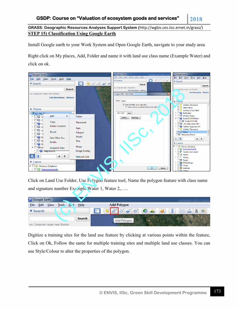
GSDP: Course on “Valuation of ecosystem goods and services” 2018 GRASS: Geographic Resources Analyses Support System (http://wgbis.ces.iisc.ernet.in/grass/)
173 © ENVIS, IISc, Green Skill Development Programme
STEP 15) Classification Using Google Earth
Install Google earth to your Work System and Open Google Earth, navigate to your study area.
Right click on My places, Add, Folder and name it with land use class name (Example Water) and
click on ok.
Click on Land Use Folder, Use Polygon feature tool, Name the polygon feature with class name
and signature number Example Water 1, Water 2,…..
Digitize a training sites for the land use feature by clicking at various points within the feature,
Click on Ok, Follow the same for multiple training sites and multiple land use classes. You can
use Style/Colour to alter the properties of the polygon.
(c) E
NVIS, I
ISc,
2018
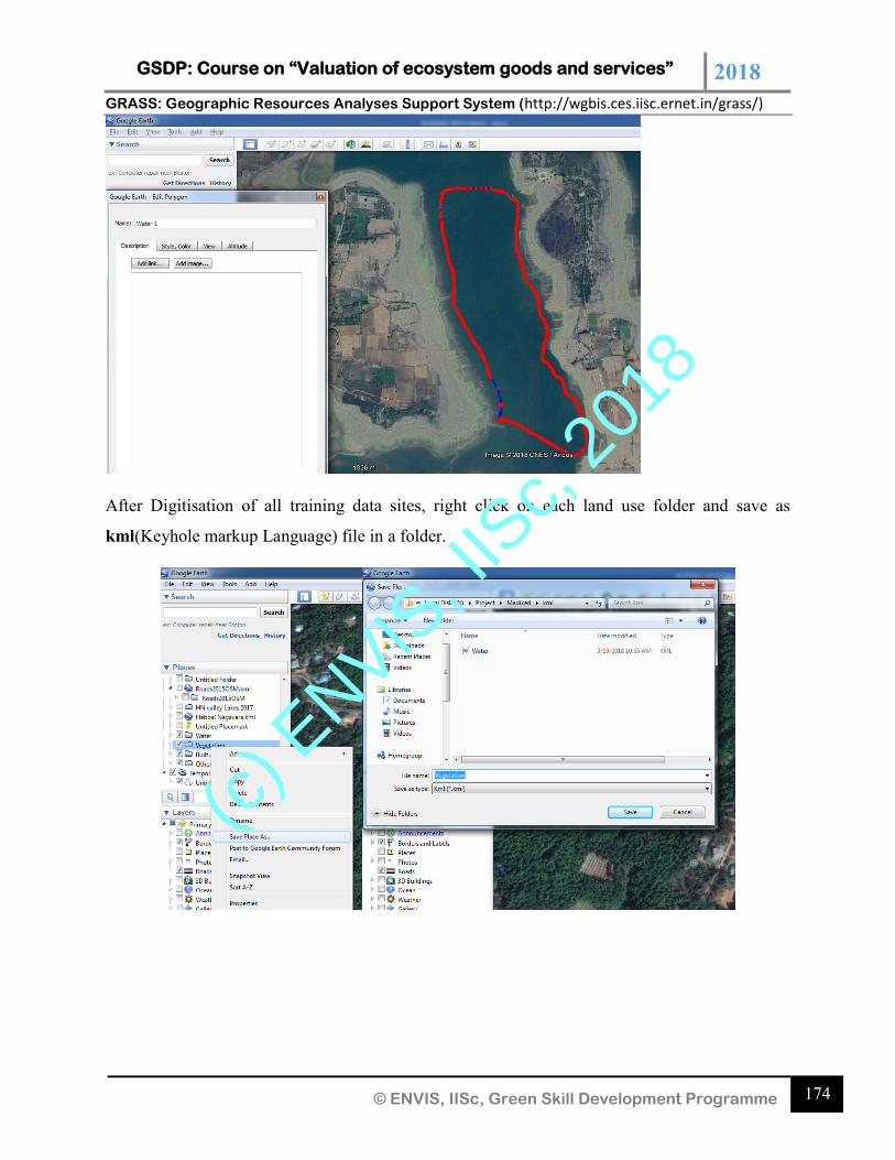
GSDP: Course on “Valuation of ecosystem goods and services” 2018 GRASS: Geographic Resources Analyses Support System (http://wgbis.ces.iisc.ernet.in/grass/)
174 © ENVIS, IISc, Green Skill Development Programme
After Digitisation of all training data sites, right click on each land use folder and save as
kml(Keyhole markup Language) file in a folder.
(c) E
NVIS, I
ISc,
2018
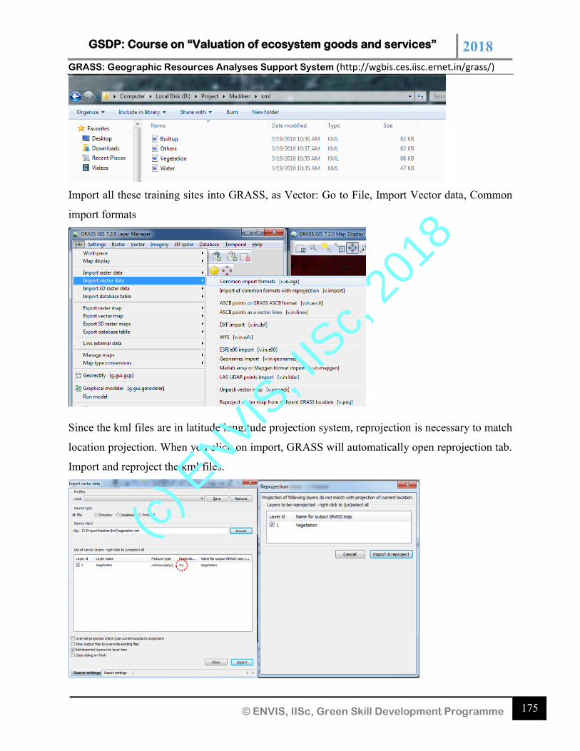
GSDP: Course on “Valuation of ecosystem goods and services” 2018 GRASS: Geographic Resources Analyses Support System (http://wgbis.ces.iisc.ernet.in/grass/)
175 © ENVIS, IISc, Green Skill Development Programme
Import all these training sites into GRASS, as Vector: Go to File, Import Vector data, Common
import formats
Since the kml files are in latitude longitude projection system, reprojection is necessary to match
location projection. When you click on import, GRASS will automatically open reprojection tab.
Import and reproject the kml files.
(c) E
NVIS, I
ISc,
2018
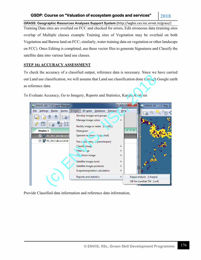
GSDP: Course on “Valuation of ecosystem goods and services” 2018 GRASS: Geographic Resources Analyses Support System (http://wgbis.ces.iisc.ernet.in/grass/)
176 © ENVIS, IISc, Green Skill Development Programme
Training Data sites are overlaid on FCC and checked for errors, Edit erroneous data (training sites
overlap of Multiple classes example Training sites of Vegetation may be overlaid on both
Vegetation and Barren land on FCC; similarly, water training data on vegetation or other landscaps
on FCC). Once Editing is completed, use these vector files to generate Signatures and Classify the
satellite data into various land use classes.
STEP 16) ACCURACY ASSESSMENT
To check the accuracy of a classified output, reference data is necessary. Since we have carried
out Land use classification, we will assume that Land use classification done through Google earth
as reference data.
To Evaluate Accuracy, Go to Imagery, Reports and Statistics, Kappa Analysis
Provide Classified data information and reference data information,
(c) E
NVIS, I
ISc,
2018
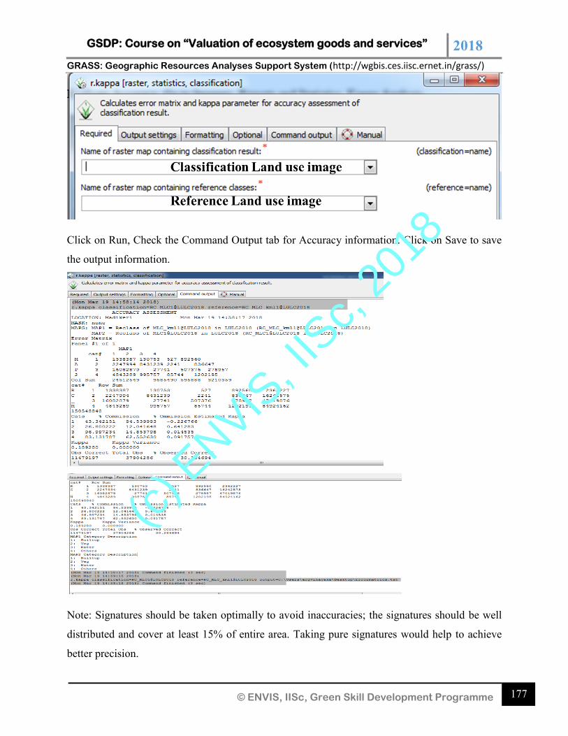
GSDP: Course on “Valuation of ecosystem goods and services” 2018 GRASS: Geographic Resources Analyses Support System (http://wgbis.ces.iisc.ernet.in/grass/)
177 © ENVIS, IISc, Green Skill Development Programme
Click on Run, Check the Command Output tab for Accuracy information. Click on Save to save
the output information.
Note: Signatures should be taken optimally to avoid inaccuracies; the signatures should be well
distributed and cover at least 15% of entire area. Taking pure signatures would help to achieve
better precision.
(c) E
NVIS, I
ISc,
2018
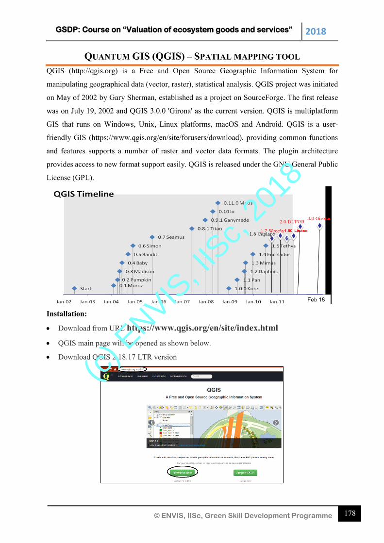
GSDP: Course on “Valuation of ecosystem goods and services” 2018
178 © ENVIS, IISc, Green Skill Development Programme
QUANTUM GIS (QGIS) – SPATIAL MAPPING TOOL
QGIS (http://qgis.org) is a Free and Open Source Geographic Information System for
manipulating geographical data (vector, raster), statistical analysis. QGIS project was initiated
on May of 2002 by Gary Sherman, established as a project on SourceForge. The first release
was on July 19, 2002 and QGIS 3.0.0 'Girona' as the current version. QGIS is multiplatform
GIS that runs on Windows, Unix, Linux platforms, macOS and Android. QGIS is a user-
friendly GIS (https://www.qgis.org/en/site/forusers/download), providing common functions
and features supports a number of raster and vector data formats. The plugin architecture
provides access to new format support easily. QGIS is released under the GNU General Public
License (GPL).
Installation:
Download from URL https://www.qgis.org/en/site/index.html
QGIS main page will be opened as shown below.
Download QGIS 2.18.17 LTR version
(c) E
NVIS, I
ISc,
2018
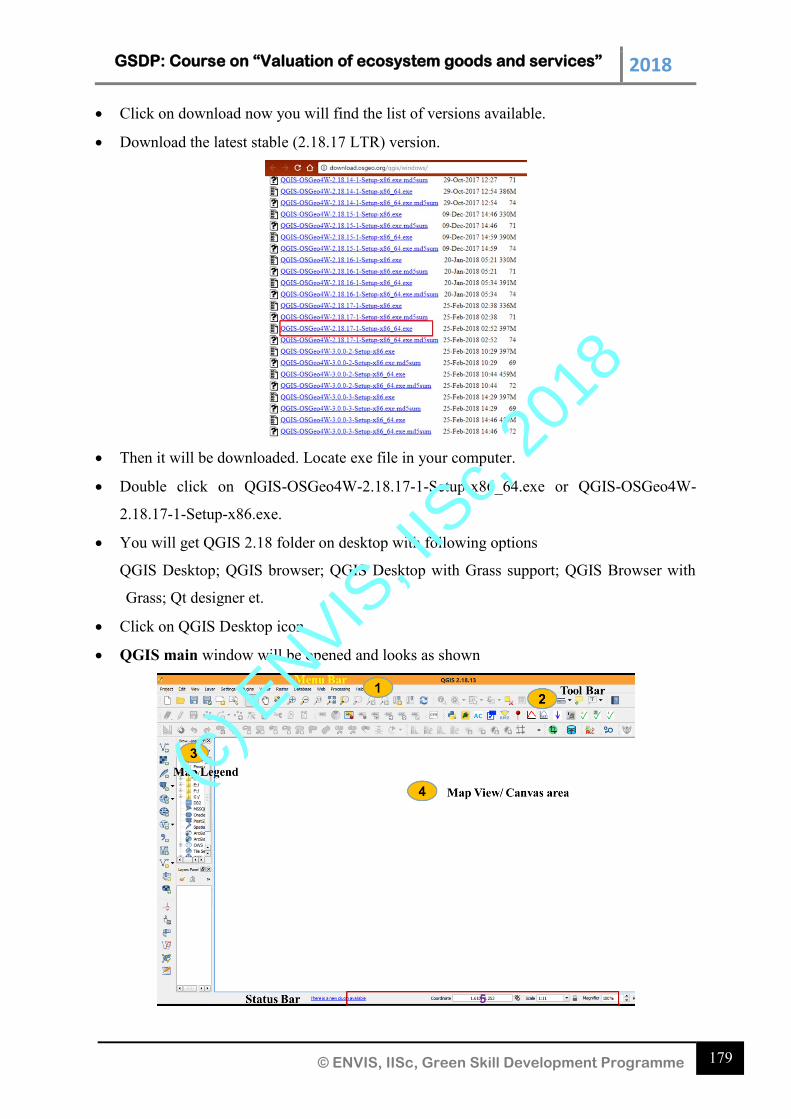
GSDP: Course on “Valuation of ecosystem goods and services” 2018
179 © ENVIS, IISc, Green Skill Development Programme
Click on download now you will find the list of versions available.
Download the latest stable (2.18.17 LTR) version.
Then it will be downloaded. Locate exe file in your computer.
Double click on QGIS-OSGeo4W-2.18.17-1-Setup-x86_64.exe or QGIS-OSGeo4W-
2.18.17-1-Setup-x86.exe.
You will get QGIS 2.18 folder on desktop with following options
QGIS Desktop; QGIS browser; QGIS Desktop with Grass support; QGIS Browser with
Grass; Qt designer et.
Click on QGIS Desktop icon.
QGIS main window will be opened and looks as shown
(c) E
NVIS, I
ISc,
2018
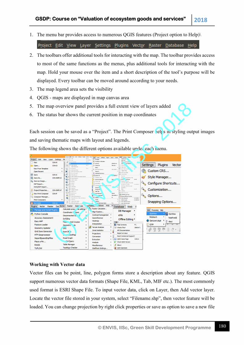
GSDP: Course on “Valuation of ecosystem goods and services” 2018
180 © ENVIS, IISc, Green Skill Development Programme
1. The menu bar provides access to numerous QGIS features (Project option to Help)\
2. The toolbars offer additional tools for interacting with the map. The toolbar provides access
to most of the same functions as the menus, plus additional tools for interacting with the
map. Hold your mouse over the item and a short description of the tool’s purpose will be
displayed. Every toolbar can be moved around according to your needs.
3. The map legend area sets the visibility
4. QGIS - maps are displayed in map canvas area
5. The map overview panel provides a full extent view of layers added
6. The status bar shows the current position in map coordinates
Each session can be saved as a “Project”. The Print Composer helps in styling output images
and saving thematic maps with layout and legends.
The following shows the different options available under each menu.
Working with Vector data
Vector files can be point, line, polygon forms store a description about any feature. QGIS
support numerous vector data formats (Shape File, KML, Tab, MIF etc.). The most commonly
used format is ESRI Shape File. To input vector data, click on Layer, then Add vector layer.
Locate the vector file stored in your system, select “Filename.shp”, then vector feature will be
loaded. You can change projection by right click properties or save as option to save a new file
(c) E
NVIS, I
ISc,
2018
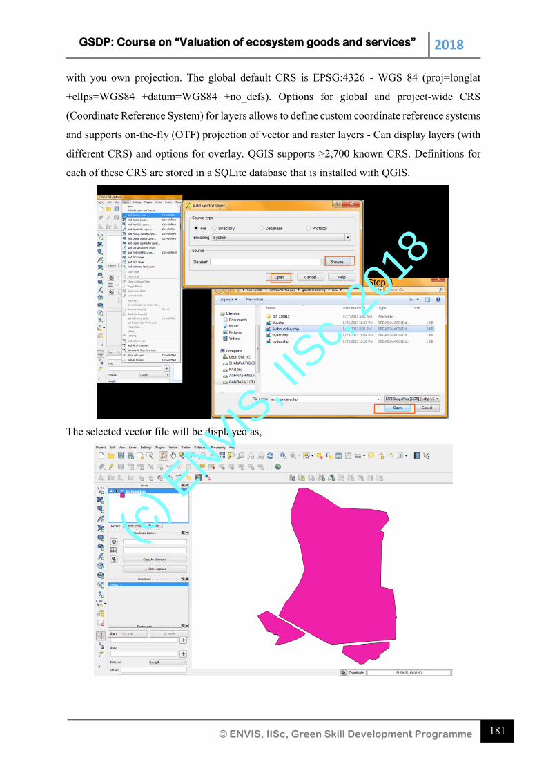
GSDP: Course on “Valuation of ecosystem goods and services” 2018
181 © ENVIS, IISc, Green Skill Development Programme
with you own projection. The global default CRS is EPSG:4326 - WGS 84 (proj=longlat
+ellps=WGS84 +datum=WGS84 +no_defs). Options for global and project-wide CRS
(Coordinate Reference System) for layers allows to define custom coordinate reference systems
and supports on-the-fly (OTF) projection of vector and raster layers - Can display layers (with
different CRS) and options for overlay. QGIS supports >2,700 known CRS. Definitions for
each of these CRS are stored in a SQLite database that is installed with QGIS.
The selected vector file will be displayed as,
(c) E
NVIS, I
ISc,
2018
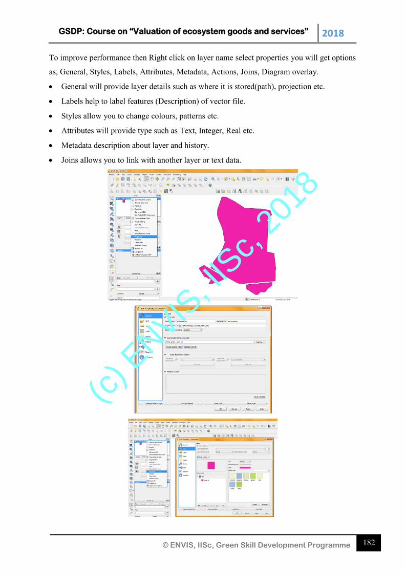
GSDP: Course on “Valuation of ecosystem goods and services” 2018
182 © ENVIS, IISc, Green Skill Development Programme
To improve performance then Right click on layer name select properties you will get options
as, General, Styles, Labels, Attributes, Metadata, Actions, Joins, Diagram overlay.
General will provide layer details such as where it is stored(path), projection etc.
Labels help to label features (Description) of vector file.
Styles allow you to change colours, patterns etc.
Attributes will provide type such as Text, Integer, Real etc.
Metadata description about layer and history.
Joins allows you to link with another layer or text data.
(c) E
NVIS, I
ISc,
2018
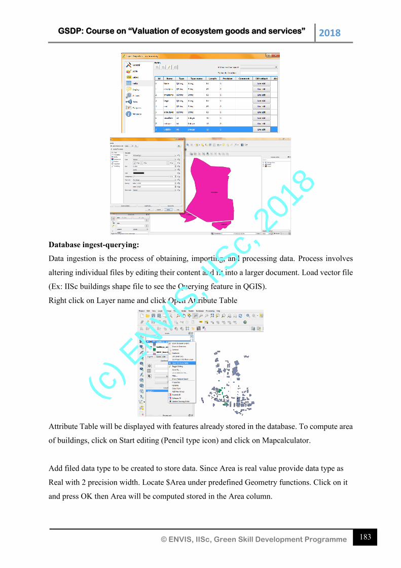
GSDP: Course on “Valuation of ecosystem goods and services” 2018
183 © ENVIS, IISc, Green Skill Development Programme
Database ingest-querying:
Data ingestion is the process of obtaining, importing, and processing data. Process involves
altering individual files by editing their content and fit into a larger document. Load vector file
(Ex: IISc buildings shape file to see the Querying feature in QGIS).
Right click on Layer name and click Open Attribute Table
Attribute Table will be displayed with features already stored in the database. To compute area
of buildings, click on Start editing (Pencil type icon) and click on Mapcalculator.
Add filed data type to be created to store data. Since Area is real value provide data type as
Real with 2 precision width. Locate $Area under predefined Geometry functions. Click on it
and press OK then Area will be computed stored in the Area column.
(c) E
NVIS, I
ISc,
2018
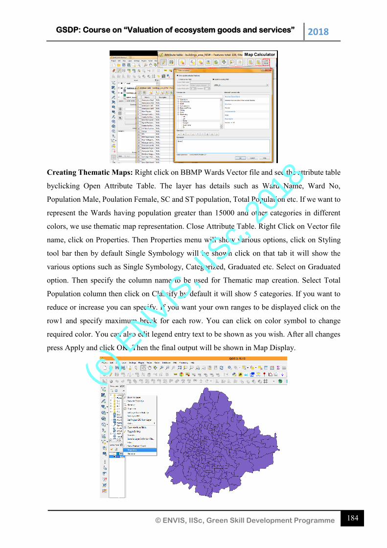
GSDP: Course on “Valuation of ecosystem goods and services” 2018
184 © ENVIS, IISc, Green Skill Development Programme
Creating Thematic Maps: Right click on BBMP Wards Vector file and see the attribute table
byclicking Open Attribute Table. The layer has details such as Ward Name, Ward No,
Population Male, Poulation Female, SC and ST population, Total Population etc. If we want to
represent the Wards having population greater than 15000 and other categories in different
colors, we use thematic map representation. Close Attribute Table. Right Click on Vector file
name, click on Properties. Then Properties menu will show various options, click on Styling
tool bar then by default Single Symbology will be shown click on that tab it will show the
various options such as Single Symbology, Categorized, Graduated etc. Select on Graduated
option. Then specify the column name to be used for Thematic map creation. Select Total
Population column then click on Classify by default it will show 5 categories. If you want to
reduce or increase you can specify. If you want your own ranges to be displayed click on the
row1 and specify maximum break for each row. You can click on color symbol to change
required color. You can also edit legend entry text to be shown as you wish. After all changes
press Apply and click OK. Then the final output will be shown in Map Display.
(c) E
NVIS, I
ISc,
2018
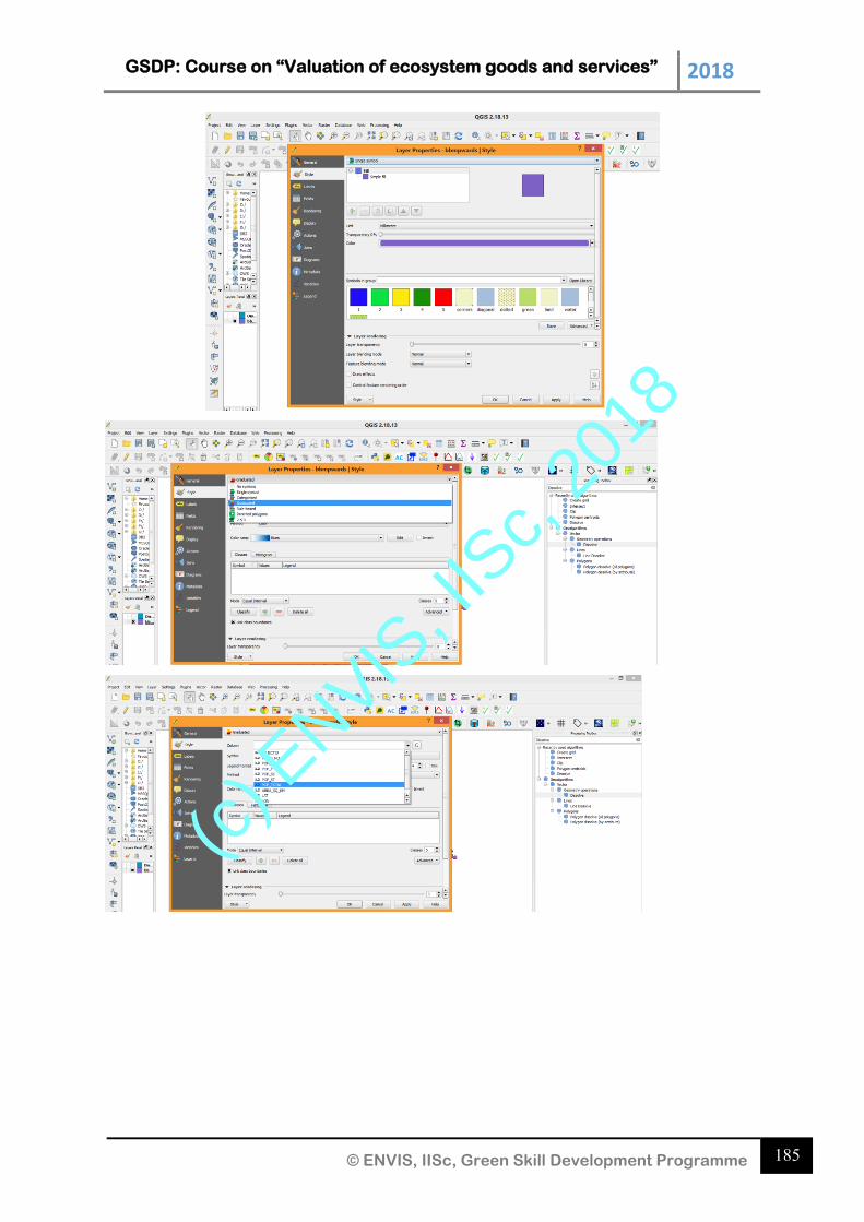
GSDP: Course on “Valuation of ecosystem goods and services” 2018
185 © ENVIS, IISc, Green Skill Development Programme
(c) E
NVIS, I
ISc,
2018
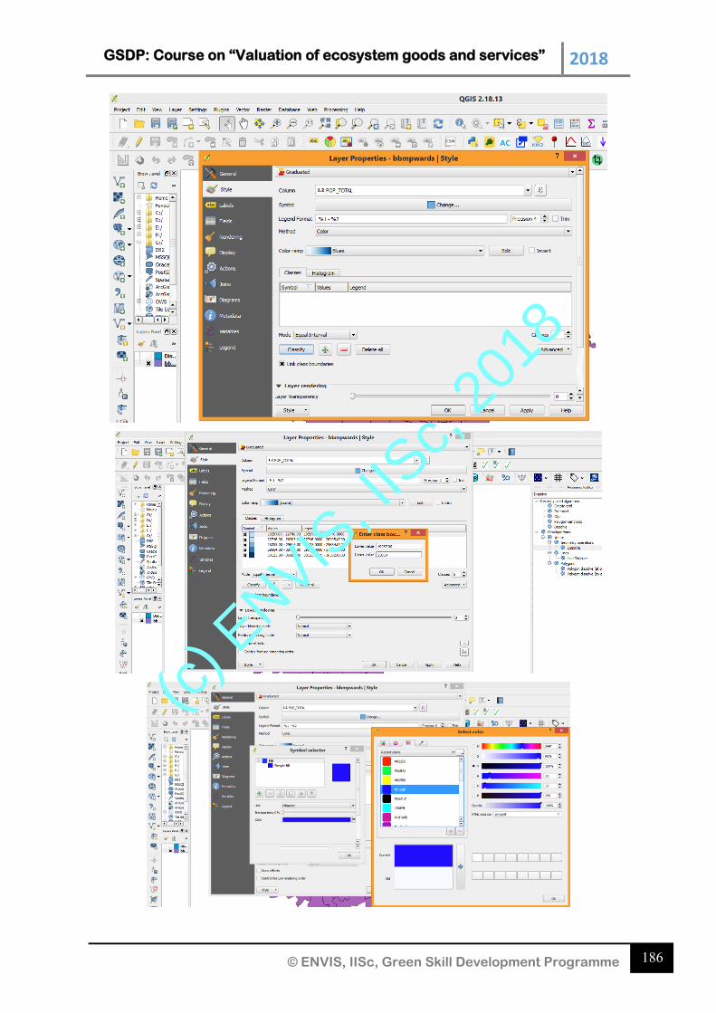
GSDP: Course on “Valuation of ecosystem goods and services” 2018
186 © ENVIS, IISc, Green Skill Development Programme
(c) E
NVIS, I
ISc,
2018
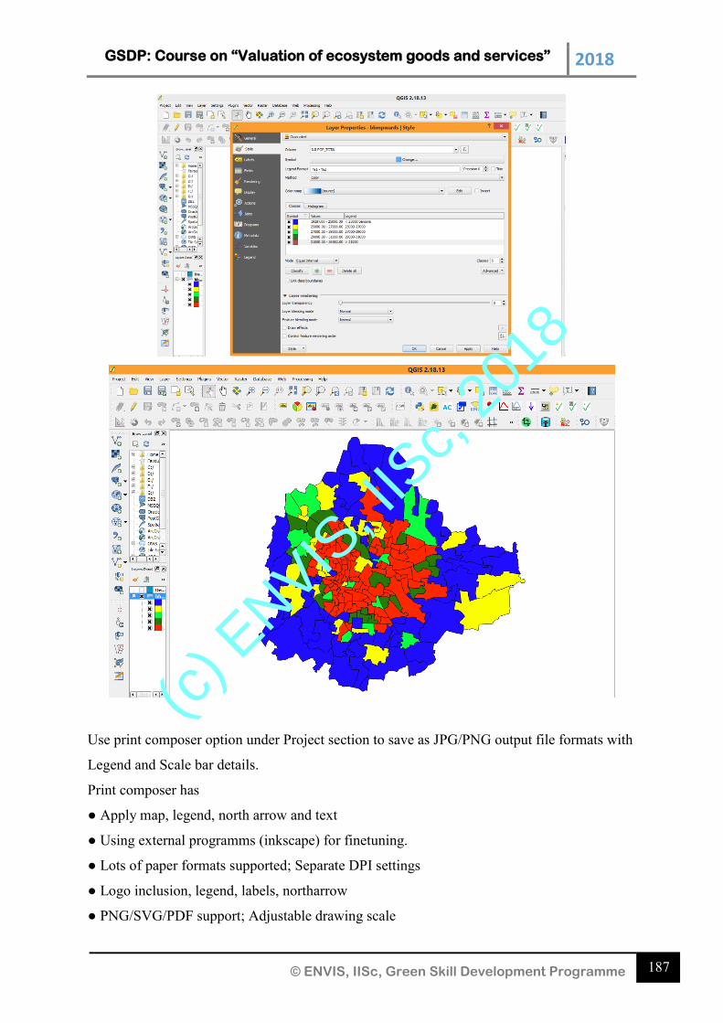
GSDP: Course on “Valuation of ecosystem goods and services” 2018
187 © ENVIS, IISc, Green Skill Development Programme
Use print composer option under Project section to save as JPG/PNG output file formats with
Legend and Scale bar details.
Print composer has
● Apply map, legend, north arrow and text
● Using external programms (inkscape) for finetuning.
● Lots of paper formats supported; Separate DPI settings
● Logo inclusion, legend, labels, northarrow
● PNG/SVG/PDF support; Adjustable drawing scale
(c) E
NVIS, I
ISc,
2018
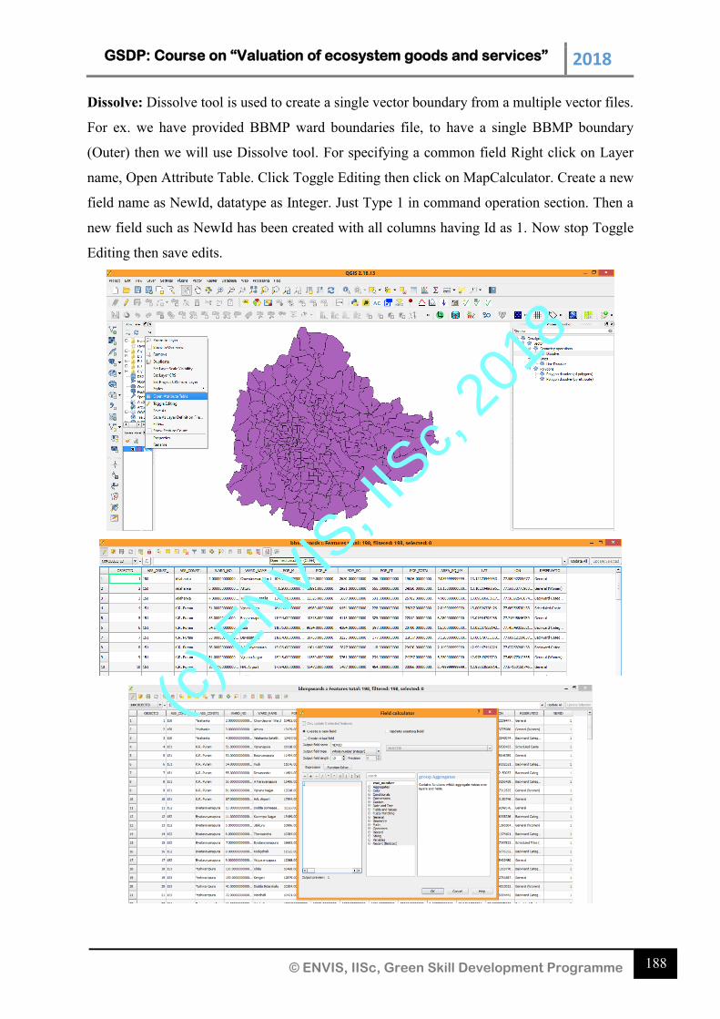
GSDP: Course on “Valuation of ecosystem goods and services” 2018
188 © ENVIS, IISc, Green Skill Development Programme
Dissolve: Dissolve tool is used to create a single vector boundary from a multiple vector files.
For ex. we have provided BBMP ward boundaries file, to have a single BBMP boundary
(Outer) then we will use Dissolve tool. For specifying a common field Right click on Layer
name, Open Attribute Table. Click Toggle Editing then click on MapCalculator. Create a new
field name as NewId, datatype as Integer. Just Type 1 in command operation section. Then a
new field such as NewId has been created with all columns having Id as 1. Now stop Toggle
Editing then save edits.
(c) E
NVIS, I
ISc,
2018
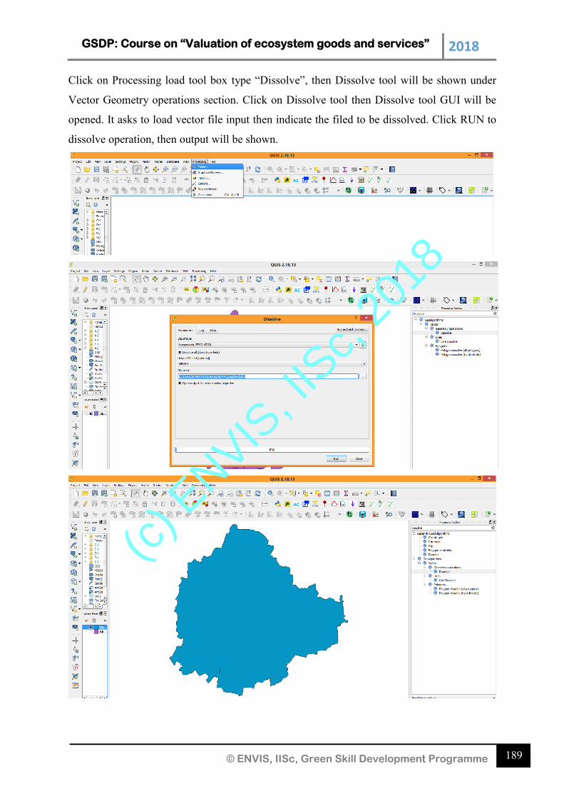
GSDP: Course on “Valuation of ecosystem goods and services” 2018
189 © ENVIS, IISc, Green Skill Development Programme
Click on Processing load tool box type “Dissolve”, then Dissolve tool will be shown under
Vector Geometry operations section. Click on Dissolve tool then Dissolve tool GUI will be
opened. It asks to load vector file input then indicate the filed to be dissolved. Click RUN to
dissolve operation, then output will be shown.
(c) E
NVIS, I
ISc,
2018
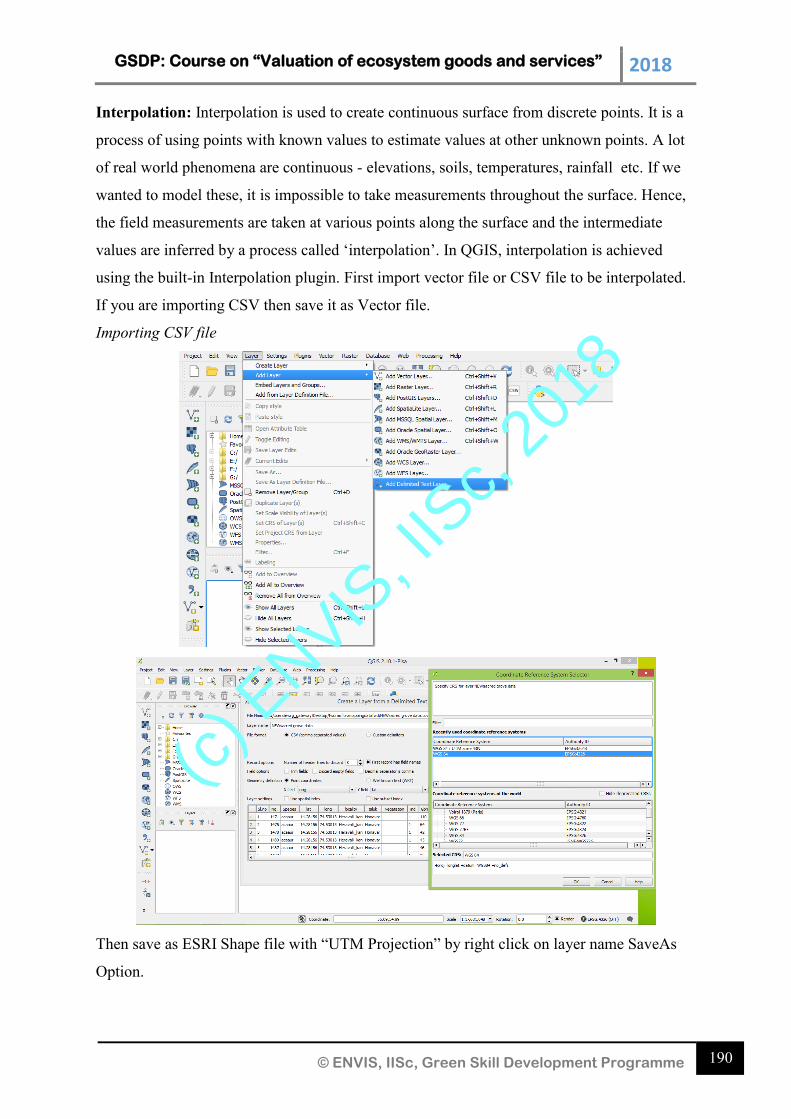
GSDP: Course on “Valuation of ecosystem goods and services” 2018
190 © ENVIS, IISc, Green Skill Development Programme
Interpolation: Interpolation is used to create continuous surface from discrete points. It is a
process of using points with known values to estimate values at other unknown points. A lot
of real world phenomena are continuous - elevations, soils, temperatures, rainfall etc. If we
wanted to model these, it is impossible to take measurements throughout the surface. Hence,
the field measurements are taken at various points along the surface and the intermediate
values are inferred by a process called ‘interpolation’. In QGIS, interpolation is achieved
using the built-in Interpolation plugin. First import vector file or CSV file to be interpolated.
If you are importing CSV then save it as Vector file.
Importing CSV file
Then save as ESRI Shape file with “UTM Projection” by right click on layer name SaveAs
Option.
(c) E
NVIS, I
ISc,
2018
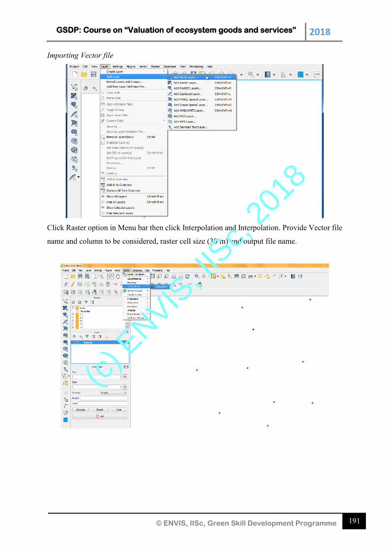
GSDP: Course on “Valuation of ecosystem goods and services” 2018
191 © ENVIS, IISc, Green Skill Development Programme
Importing Vector file
Click Raster option in Menu bar then click Interpolation and Interpolation. Provide Vector file
name and column to be considered, raster cell size (30 m) and output file name.
(c) E
NVIS, I
ISc,
2018
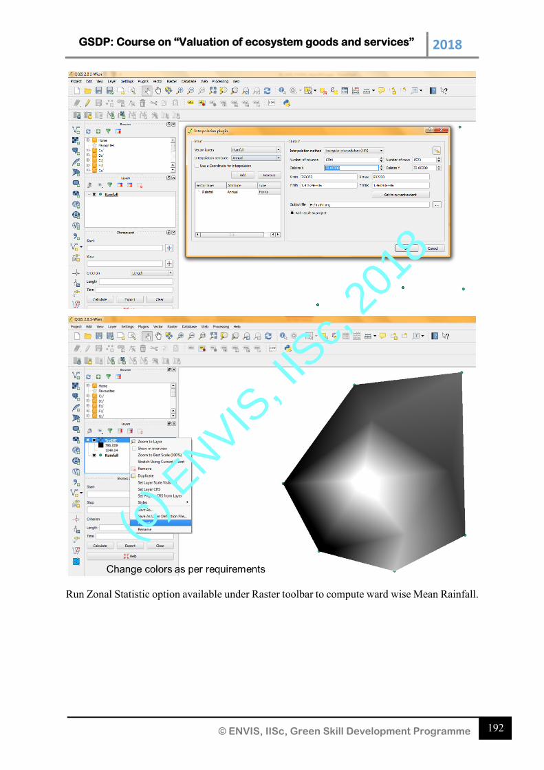
GSDP: Course on “Valuation of ecosystem goods and services” 2018
192 © ENVIS, IISc, Green Skill Development Programme
Run Zonal Statistic option available under Raster toolbar to compute ward wise Mean Rainfall.
(c) E
NVIS, I
ISc,
2018
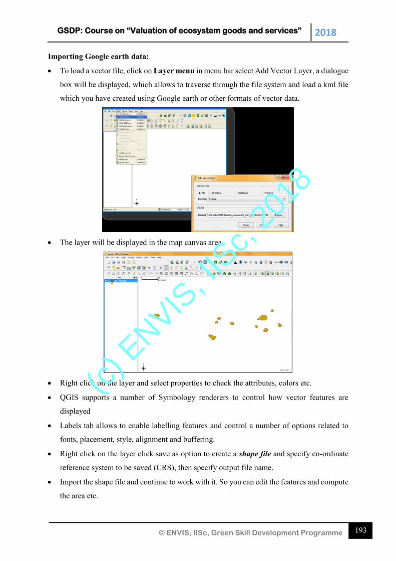
GSDP: Course on “Valuation of ecosystem goods and services” 2018
193 © ENVIS, IISc, Green Skill Development Programme
Importing Google earth data:
To load a vector file, click on Layer menu in menu bar select Add Vector Layer, a dialogue
box will be displayed, which allows to traverse through the file system and load a kml file
which you have created using Google earth or other formats of vector data.
The layer will be displayed in the map canvas area.
Right click on the layer and select properties to check the attributes, colors etc.
QGIS supports a number of Symbology renderers to control how vector features are
displayed
Labels tab allows to enable labelling features and control a number of options related to
fonts, placement, style, alignment and buffering.
Right click on the layer click save as option to create a shape file and specify co-ordinate
reference system to be saved (CRS), then specify output file name.
Import the shape file and continue to work with it. So you can edit the features and compute
the area etc.
(c) E
NVIS, I
ISc,
2018
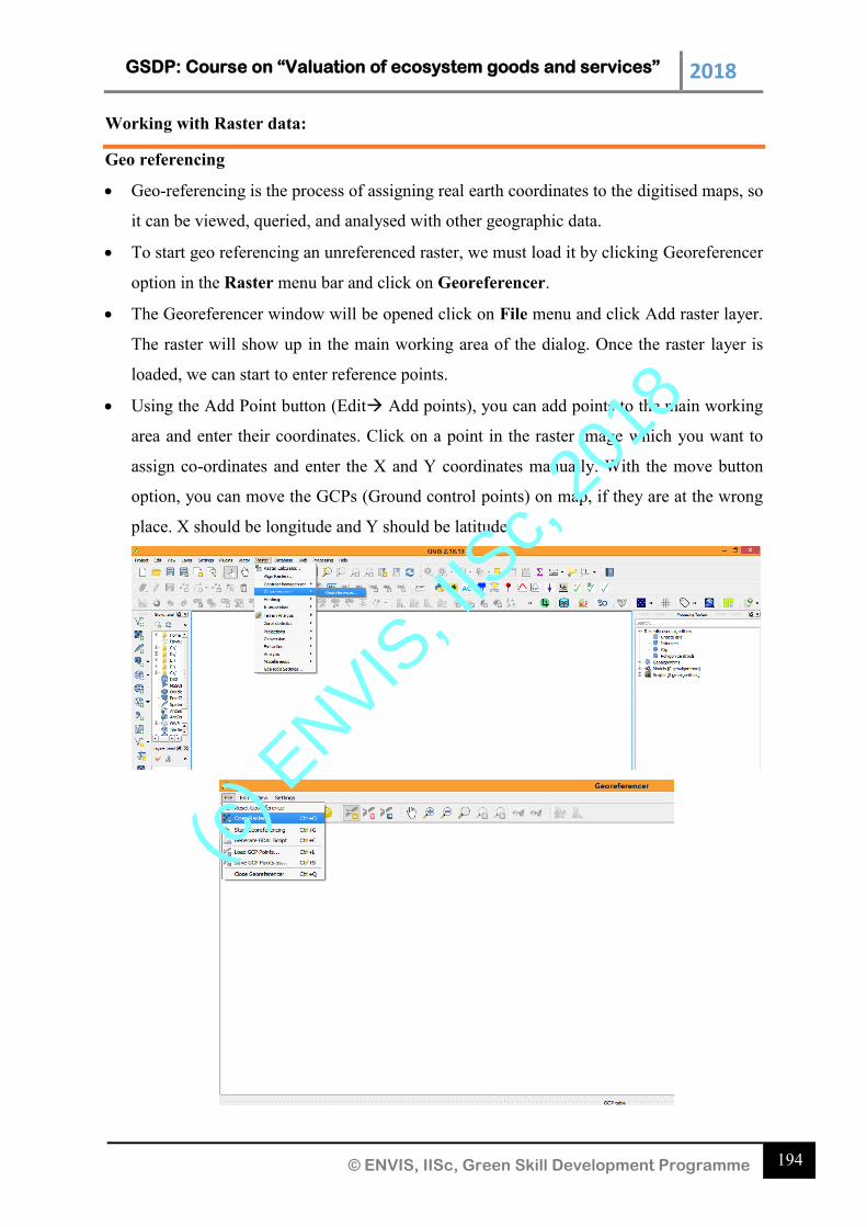
GSDP: Course on “Valuation of ecosystem goods and services” 2018
194 © ENVIS, IISc, Green Skill Development Programme
Working with Raster data:
Geo referencing
Geo-referencing is the process of assigning real earth coordinates to the digitised maps, so
it can be viewed, queried, and analysed with other geographic data.
To start geo referencing an unreferenced raster, we must load it by clicking Georeferencer
option in the Raster menu bar and click on Georeferencer.
The Georeferencer window will be opened click on File menu and click Add raster layer.
The raster will show up in the main working area of the dialog. Once the raster layer is
loaded, we can start to enter reference points.
Using the Add Point button (Edit Add points), you can add points to the main working
area and enter their coordinates. Click on a point in the raster image which you want to
assign co-ordinates and enter the X and Y coordinates manually. With the move button
option, you can move the GCPs (Ground control points) on map, if they are at the wrong
place. X should be longitude and Y should be latitude.
(c) E
NVIS, I
ISc,
2018
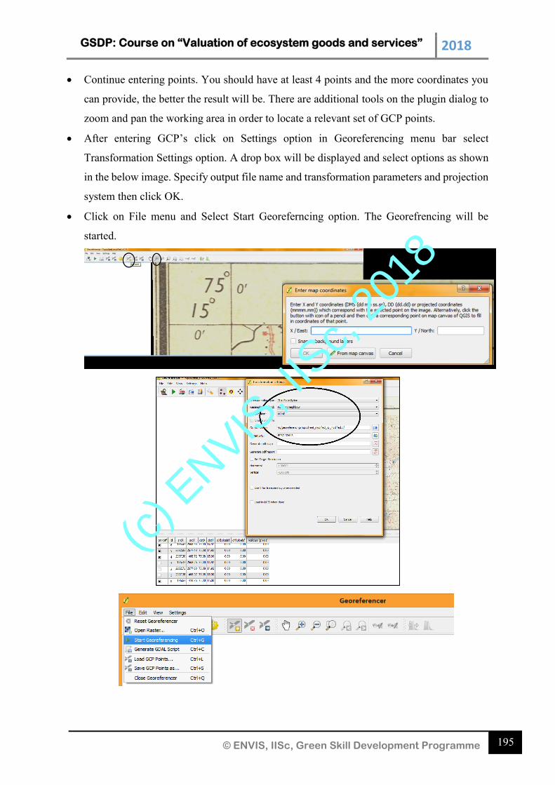
GSDP: Course on “Valuation of ecosystem goods and services” 2018
195 © ENVIS, IISc, Green Skill Development Programme
Continue entering points. You should have at least 4 points and the more coordinates you
can provide, the better the result will be. There are additional tools on the plugin dialog to
zoom and pan the working area in order to locate a relevant set of GCP points.
After entering GCP’s click on Settings option in Georeferencing menu bar select
Transformation Settings option. A drop box will be displayed and select options as shown
in the below image. Specify output file name and transformation parameters and projection
system then click OK.
Click on File menu and Select Start Georeferncing option. The Georefrencing will be
started.
(c) E
NVIS, I
ISc,
2018
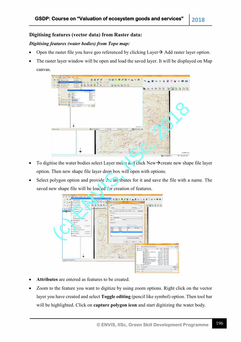
GSDP: Course on “Valuation of ecosystem goods and services” 2018
196 © ENVIS, IISc, Green Skill Development Programme
Digitising features (vector data) from Raster data:
Digitising features (water bodies) from Topo map:
Open the raster file you have geo referenced by clicking Layer Add raster layer option.
The raster layer window will be open and load the saved layer. It will be displayed on Map
canvas.
To digitise the water bodies select Layer menu and click Newcreate new shape file layer
option. Then new shape file layer drop box will open with options.
Select polygon option and provide the attributes for it and save the file with a name. The
saved new shape file will be loaded for creation of features.
Attributes are entered as features to be created.
Zoom to the feature you want to digitize by using zoom options. Right click on the vector
layer you have created and select Toggle editing (pencil like symbol) option. Then tool bar
will be highlighted. Click on capture polygon icon and start digitizing the water body.
(c) E
NVIS, I
ISc,
2018
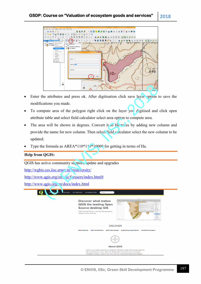
GSDP: Course on “Valuation of ecosystem goods and services” 2018
197 © ENVIS, IISc, Green Skill Development Programme
Enter the attributes and press ok. After digitisation click save layer option to save the
modifications you made.
To compute area of the polygon right click on the layer you digitised and click open
attribute table and select field calculator select area option to compute area.
The area will be shown in degrees. Convert it to Hectares by adding new column and
provide the name for new column. Then select field calculator select the new column to be
updated.
Type the formula as AREA*110*110*10000 for getting in terms of Ha.
Help from QGIS:
QGIS has active community support, update and upgrades
http://wgbis.ces.iisc.ernet.in/biodiversity/
http://www.qgis.org/en/site/forusers/index.html#
http://www.qgis.org/en/docs/index.html
(c) E
NVIS, I
ISc,
2018
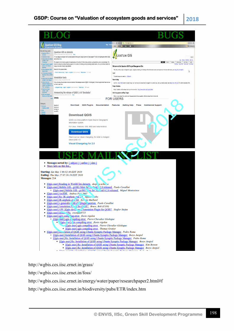
GSDP: Course on “Valuation of ecosystem goods and services” 2018
198 © ENVIS, IISc, Green Skill Development Programme
http://wgbis.ces.iisc.ernet.in/grass/
http://wgbis.ces.iisc.ernet.in/foss/
http://wgbis.ces.iisc.ernet.in/energy/water/paper/researchpaper2.html#f
http://wgbis.ces.iisc.ernet.in/biodiversity/pubs/ETR/index.htm
(c) E
NVIS, I
ISc,
2018
GSDP: Course on “Valuation of ecosystem goods and services” 2018
199 © ENVIS, IISc, Green Skill Development Programme
10. Ecosystem, LULC Analyses, Ecological Sampling
Reference:
1. Ramachandra T.V., Subash Chandran M D., Gururaja K V and Sreekantha, 2007. Cumulative
Environmental Impact Assessment, Nova Science Publishers, New York.
2. Ali, Sameer, G. R. Rao, Divakar K. Mesta, Sreekantha, Mukri Vishnu, M. D. Subash Chandran,
K. V. Gururaja, N. V. Joshi, and T. V. Ramachandra. Ecological Status of Sharavathi Valley
Wildlife Sanctuary. Prism Books Pvt Ltd., Bangalore, 2007
Ecosystems have several fundamental characteristics. First, an ecosystem has structure - non-
living (abiotic) and living parts (biotic). Non-living parts include rock, water and air. The living
part is the community, which is a set of interacting species. Second, an ecosystem has
processes, -energy flows and material recycling. Third, an ecosystem changes over time and
can undergo development through a process called succession. Ecosystems have natural
boundaries such as forests, rivers, or mountains; however, man-made constructions such as
highways, buildings, or sidewalks can also be considered boundaries to smaller ecosystems.
STRUCTURE OF THE ECOSYSTEM: From the structural point of view, all ecosystems
consist of the following basic components:
Abiotic component: Abiotic components of the ecosystem, include basic inorganic
molecules elements and compounds such as soil, water, oxygen, calcium, carbonates,
phosphates and a variety of organic compounds. The physical factors like light,
temperature, water, atmospheric gases, etc. are also included in them.
Biotic component: The biotic component includes all living organisms in the environmental
system. An ecosystem consists basically of the following.
Producers: Producers are organisms, which are able to manufacture organic
compounds from inorganic substances from their environment. Green plants are able to
do this by the means of photosynthesis, where the sun provides the necessary energy.
Therefore, these green plants are the autotrophic organisms or primary producers in
most ecosystems.
Consumers: These are organisms, which cannot make organic compounds from
inorganic substances. They are dependant upon autotrophic organisms and are the
consumers or heterotrophic organisms in an ecosystem. The consumers are further
subdivided according to their diet, into:
Herbivores or plant eaters which are the primary consumers, e.g. cows, giraffes,
elephants, etc;
Carnivores or meat eaters which are the secondary consumers; some carnivores are
called predators (eg. lions, leopard, fish eagle, etc) which catch their prey, kill it
and then eat it; others are called scavengers ( eg. vultures) which usually eat what
is left by the predators;
Omnivores eat plant and animal material and can be primary, secondary and
tertiary consumers simultaneously; a human being is a good example of an
omnivore.
Decomposers: They are the living components of the ecosystem such as bacteria
and fungi and obtain their energy by decomposing the corpses and other dead parts
(c) E
NVIS, I
ISc,
2018
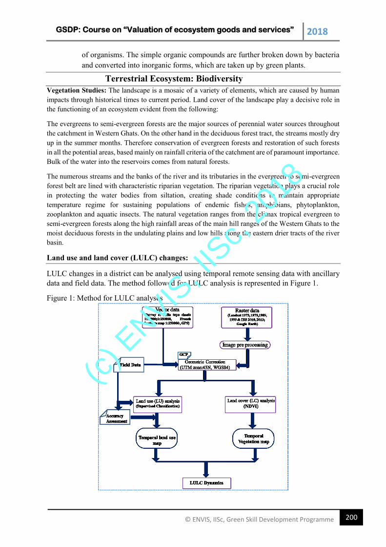
GSDP: Course on “Valuation of ecosystem goods and services” 2018
200 © ENVIS, IISc, Green Skill Development Programme
of organisms. The simple organic compounds are further broken down by bacteria
and converted into inorganic forms, which are taken up by green plants.
Terrestrial Ecosystem: Biodiversity
Vegetation Studies: The landscape is a mosaic of a variety of elements, which are caused by human
impacts through historical times to current period. Land cover of the landscape play a decisive role in
the functioning of an ecosystem evident from the following:
The evergreens to semi-evergreen forests are the major sources of perennial water sources throughout
the catchment in Western Ghats. On the other hand in the deciduous forest tract, the streams mostly dry
up in the summer months. Therefore conservation of evergreen forests and restoration of such forests
in all the potential areas, based mainly on rainfall criteria of the catchment are of paramount importance.
Bulk of the water into the reservoirs comes from natural forests.
The numerous streams and the banks of the river and its tributaries in the evergreen to semi-evergreen
forest belt are lined with characteristic riparian vegetation. The riparian vegetation plays a crucial role
in protecting the water bodies from siltation, creating shade conditions to maintain appropriate
temperature regime for sustaining populations of endemic fishes, amphibians, phytoplankton,
zooplankton and aquatic insects. The natural vegetation ranges from the climax tropical evergreen to
semi-evergreen forests along the high rainfall areas of the main hill ranges of the Western Ghats to the
moist deciduous forests in the undulating plains and low hills along the eastern drier tracts of the river
basin.
Land use and land cover (LULC) changes:
LULC changes in a district can be analysed using temporal remote sensing data with ancillary
data and field data. The method followed for LULC analysis is represented in Figure 1.
Figure 1: Method for LULC analyses
(c) E
NVIS, I
ISc,
2018
GSDP: Course on “Valuation of ecosystem goods and services” 2018
201 © ENVIS, IISc, Green Skill Development Programme
Remote sensing data: Temporal remote sensing data of Landsat satellite are available at
public domains at Global Land Cover Facility (GLCF) (http://www.glcf.umd.edu/index.shtml)
and United States Geological Survey (USGS) Earth Explorer
(http://edcsns17.cr.usgs.gov/NewEarthExplorer/). Base layers such as district, taluk boundary,
stream network, etc. are to be digitised from The Survey of India (SOI) topographic maps of
1:50000 and 1:250000 scales (http://surveyofindia.gov.in). Ground control points to register
and geo-correct remote sensing data are to be collected using hand held pre-calibrated GPS
(Global Positioning System), Survey of India topographic maps and Google earth
(http://earth.google.com, http://bhuvan.nrsc.gov.in).
Ancillary data: Ancillary data include cadastral revenue maps (1:6000), the Survey of India
(SOI) topographic maps (1:50000 and 1:250000 scales), vegetation map of South India
developed by French Institute (1986) of scale 1:250000. Topographic maps provides ground
control points (GCP’s) to rectify remote sensing data and scanned paper maps. Vegetation map
of South India (1986) of scale 1:250000 (Pascal, 1986) is useful to identify various forest cover
types and classify RS data of 1980’s. Other ancillary data includes land cover maps,
administration boundary data, transportation data (road network), etc. Pre-calibrated GPS
(Global Positioning System - Garmin GPS units) are useful in field data collection, required
for RS data classification as well as for validation.
Land use analysis: Land use analysis involves (i) generation of False Color Composite (FCC)
of remote sensing data (bands–green, red and NIR). This composite image helps in locating
heterogeneous patches in the landscape, (ii) selection of training polygons by covering 15% of
the study area (polygons are uniformly distributed over the entire study area) (iii) loading
these training polygons co-ordinates into pre-calibrated GPS, (vi) collection of the
corresponding attribute data (land use types) for these polygons from the field. GPS helped
in locating respective training polygons in the field, (iv) supplementing this information with
Google Earth and (v) 60% of the training data has been used for classification, while
the balance is used for validation or accuracy assessment. The land use analysis was done
using supervised classification technique based on Gaussian maximum likelihood algorithm
with training data (collected from field using GPS).
Computation of Area under intact forests/Interrior forests: Fragmentation of forests at the
pixel level are estimated through the computation of Pf (the ratio of the number of pixels that
are forested to the total number of non-water pixels in the window) as given in equations 1. If
Pf = 1, then that pixel belongs to intact forests
Pf = Proportion of number of forest pixels / Total number of non ‒ Water pixels in window
(1)
Pf are computed through a moving window of 5 x 5 pixels, given that the results of the
model are scale-dependent and threshold dependent.
(c) E
NVIS, I
ISc,
2018
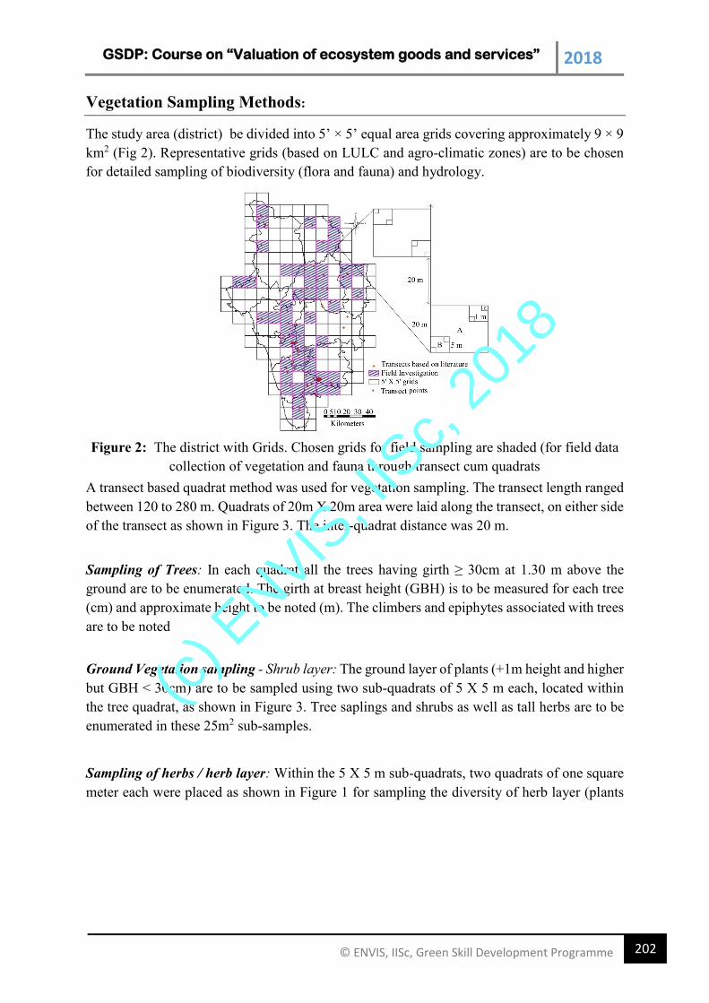
GSDP: Course on “Valuation of ecosystem goods and services” 2018
202 © ENVIS, IISc, Green Skill Development Programme
Vegetation Sampling Methods:
The study area (district) be divided into 5’ × 5’ equal area grids covering approximately 9 × 9
km2 (Fig 2). Representative grids (based on LULC and agro-climatic zones) are to be chosen
for detailed sampling of biodiversity (flora and fauna) and hydrology.
Figure 2: The district with Grids. Chosen grids for field sampling are shaded (for field data
collection of vegetation and fauna through transect cum quadrats
A transect based quadrat method was used for vegetation sampling. The transect length ranged
between 120 to 280 m. Quadrats of 20m X 20m area were laid along the transect, on either side
of the transect as shown in Figure 3. The inter-quadrat distance was 20 m.
Sampling of Trees: In each quadrat all the trees having girth ≥ 30cm at 1.30 m above the
ground are to be enumerated. The girth at breast height (GBH) is to be measured for each tree
(cm) and approximate height to be noted (m). The climbers and epiphytes associated with trees
are to be noted
Ground Vegetation sampling - Shrub layer: The ground layer of plants (+1m height and higher
but GBH < 30cm) are to be sampled using two sub-quadrats of 5 X 5 m each, located within
the tree quadrat, as shown in Figure 3. Tree saplings and shrubs as well as tall herbs are to be
enumerated in these 25m2 sub-samples.
Sampling of herbs / herb layer: Within the 5 X 5 m sub-quadrats, two quadrats of one square
meter each were placed as shown in Figure 1 for sampling the diversity of herb layer (plants
(c) E
NVIS, I
ISc,
2018
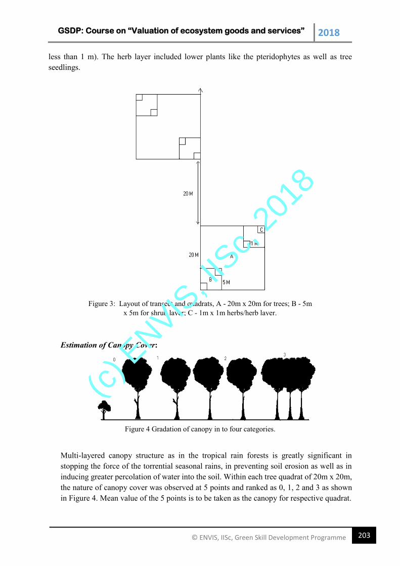
GSDP: Course on “Valuation of ecosystem goods and services” 2018
203 © ENVIS, IISc, Green Skill Development Programme
less than 1 m). The herb layer included lower plants like the pteridophytes as well as tree
seedlings.
Estimation of Canopy Cover:
Figure 4 Gradation of canopy in to four categories.
Multi-layered canopy structure as in the tropical rain forests is greatly significant in
stopping the force of the torrential seasonal rains, in preventing soil erosion as well as in
inducing greater percolation of water into the soil. Within each tree quadrat of 20m x 20m,
the nature of canopy cover was observed at 5 points and ranked as 0, 1, 2 and 3 as shown
in Figure 4. Mean value of the 5 points is to be taken as the canopy for respective quadrat.
Figure 3: Layout of transect and quadrats, A - 20m x 20m for trees; B - 5m
x 5m for shrub layer; C - 1m x 1m herbs/herb layer.
(c) E
NVIS, I
ISc,
2018
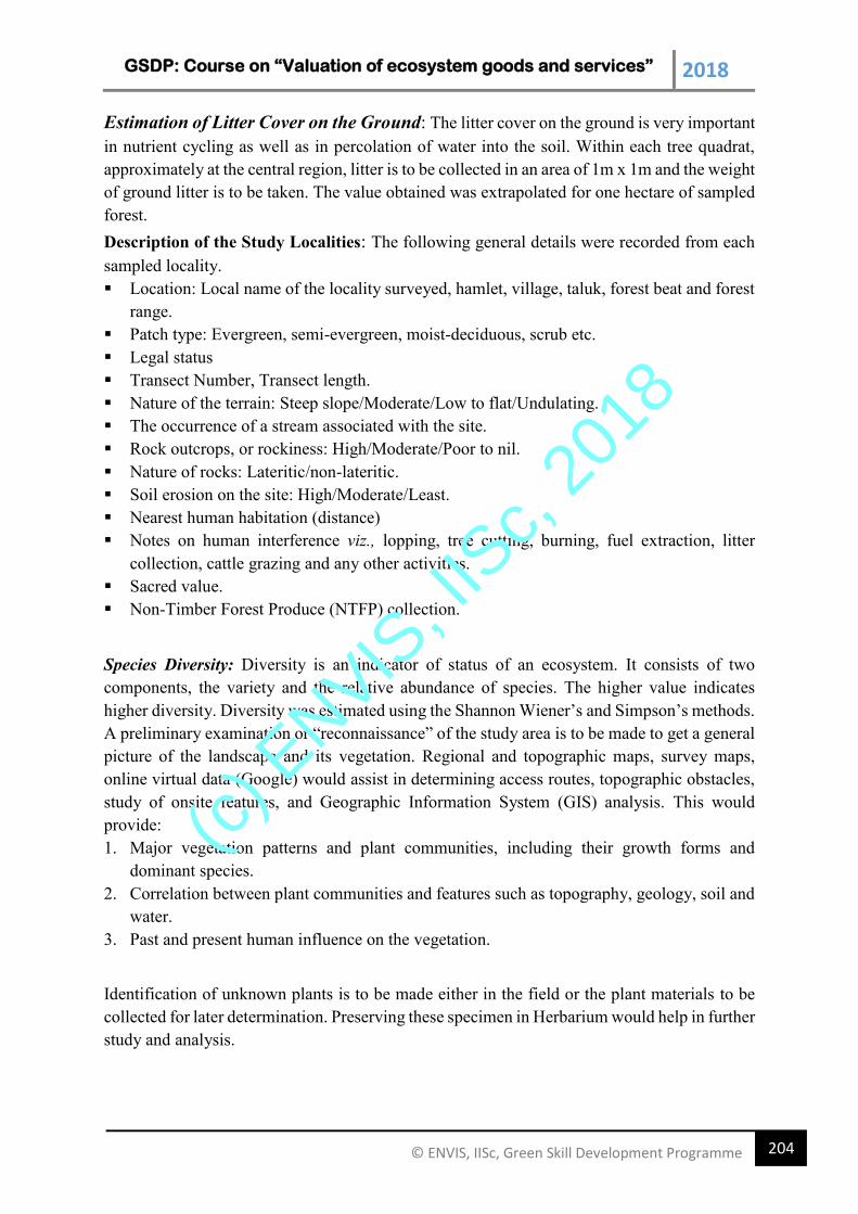
GSDP: Course on “Valuation of ecosystem goods and services” 2018
204 © ENVIS, IISc, Green Skill Development Programme
Estimation of Litter Cover on the Ground: The litter cover on the ground is very important
in nutrient cycling as well as in percolation of water into the soil. Within each tree quadrat,
approximately at the central region, litter is to be collected in an area of 1m x 1m and the weight
of ground litter is to be taken. The value obtained was extrapolated for one hectare of sampled
forest.
Description of the Study Localities: The following general details were recorded from each
sampled locality.
Location: Local name of the locality surveyed, hamlet, village, taluk, forest beat and forest
range.
Patch type: Evergreen, semi-evergreen, moist-deciduous, scrub etc.
Legal status
Transect Number, Transect length.
Nature of the terrain: Steep slope/Moderate/Low to flat/Undulating.
The occurrence of a stream associated with the site.
Rock outcrops, or rockiness: High/Moderate/Poor to nil.
Nature of rocks: Lateritic/non-lateritic.
Soil erosion on the site: High/Moderate/Least.
Nearest human habitation (distance)
Notes on human interference viz., lopping, tree cutting, burning, fuel extraction, litter
collection, cattle grazing and any other activities.
Sacred value.
Non-Timber Forest Produce (NTFP) collection.
Species Diversity: Diversity is an indicator of status of an ecosystem. It consists of two
components, the variety and the relative abundance of species. The higher value indicates
higher diversity. Diversity was estimated using the Shannon Wiener’s and Simpson’s methods.
A preliminary examination or “reconnaissance” of the study area is to be made to get a general
picture of the landscape and its vegetation. Regional and topographic maps, survey maps,
online virtual data (Google) would assist in determining access routes, topographic obstacles,
study of onsite features, and Geographic Information System (GIS) analysis. This would
provide:
1. Major vegetation patterns and plant communities, including their growth forms and
dominant species.
2. Correlation between plant communities and features such as topography, geology, soil and
water.
3. Past and present human influence on the vegetation.
Identification of unknown plants is to be made either in the field or the plant materials to be
collected for later determination. Preserving these specimen in Herbarium would help in further
study and analysis.
(c) E
NVIS, I
ISc,
2018
GSDP: Course on “Valuation of ecosystem goods and services” 2018
205 © ENVIS, IISc, Green Skill Development Programme
Ecological Measurements
A number of basic measurements help in describing population and communities. Among these
are density, frequency, coverage and biomass. Other important ecological measurements such
as population distribution, species diversity and productivity are made from these.
Density: In ecological population studies, numbers of individuals provide basic information.
Abundance (N) is the number of individuals in a given area and density (D) is the number
expressed per unit area or unit volume. For example, a species may have an abundance of 100
individuals in a particular area. If the total area were 2.5 hectares, then the density of this
species would be 40 per hectare (40/ha).
Density is the number of organisms per unit area or unit volume. Much of the area may be
habitat unsuitable for that species. Therefore it may be more meaningful to speak of the number
per unit habitable area. Thus, in the above example of 100 individuals in 2.5 hectares, if only
half the area provides suitable habitat for the species in question, then the species would have
an ecological density of 80 per hectare (80/ha).
A problem sometimes encountered in plant sampling is the determination of individuals. When
plants are growing in clumps or are producing vegetatively from underground rhizomes the
common concept of the individual falters. Then, the individual shoots or stems must be
counted; or, if the plants are growing in distinct clumps, whole clump is treated as an individual.
In many kinds of faunal sampling, accurate and absolute density determinations often are
difficult or impossible to obtain. However, if a standardised sampling procedure is used, then
at least an index of density (ID) may be calculated and used for comparative purposes. Such an
index might be the number of individuals per unit of habitat or the number per unit area.
Sometimes this is called population density. For example, the number per unit of habitat might
be the number of beetles per leaf or the number of parasites per host organism. Density
expressed per unit of sampling effort might be the number of grasshoppers per sweep of a net,
the number of fish caught per hour, the number of birds seen per kilometre of walking, or the
number of mice caught per trap per night.
In comparative studies, one wants to know the number of individuals relative to other
populations or relative to the same population at other times. Relative species density (RD) is
important in community studies. Relative species density is the total number of individuals of
all species. Example, if there are 50 trees in a given area, and 30 of them are Lophopetalum,
then the relative species density of Lophopetalum is 30/50 or 60%.
Relative population density is the number of individuals of a given species from one location
or time expressed as a proportion of the total number of individuals of that species for all
locations or times sampled. If one caught 10 locusts with 100 sweeps of a collecting net in July
of one year and 70 locusts in the same location with identical sweeping effort in September,
the relative density for July would be 10/80 or 0.125 and September 70/80 or 0.875
(c) E
NVIS, I
ISc,
2018
GSDP: Course on “Valuation of ecosystem goods and services” 2018
206 © ENVIS, IISc, Green Skill Development Programme
Frequency: Frequency (f) is the number of times a given event occurs. In many studies, the
term frequency indicates the number of samples in which a species occurs. This is expressed
as the proportion of the total number of samples taken that contains the species in question.
Thus, if a species were found in 7 out of 10 samples taken, it would have a frequency of 7/10
or 0.7. This is same as saying the probability of finding that species in a sample is 0.7. Since
frequency is sensitive to distribution patterns of individuals, it is also useful in describing and
testing such patterns. The relative frequency (RF) is the ratio of the number of individuals of a
particular species divided by the sum of the frequencies of the species in the community.
Basal Area: The basal area for a tree has been calculated for each transect based on the girth
measured using the formula (GBH)²/4π, which is summed for a quadrat and transect. The value
arrived has been extrapolated to a hectare so as to make standard comparisons with other
tropical forests. For sub-basins the basal area of respective sampled localities were pooled
based on different vegetation types and then the value was extrapolated for a hectare of sampled
forest.
Importance Value Index: The Importance Value Index gives an overall picture of the
importance of the species in the community. It considers the relative values of density,
frequency and basal area in a given sample.
Forest Classification: The forest has been classified as Evergreen, Semi-evergreen and Moist
deciduous based on the percentage of evergreens present in the sampled localities (Table 1).
Table 1Classification of vegetation.
Vegetation type Evergreen trees (%)
Evergreen 90 to 100
Semi-evergreen 50 to 90
Moist deciduous Less than 50
Endemic Species: Endemic species are species with restricted range of distribution. A taxon
is considered as endemic if confined to a particular area through historical, ecological or
physiological reasons. At the global level endemic areas are of high conservation priority
because these species can never be replaced if they are lost. The Western Ghats endemism is
of high conservation value. During field observations, it was noticed that the endemic
vegetation patches were more associated with perennial streams and other damp soils.
The geographical distributions of all plant species identified were listed with the help of the
flora (district flora publications such as flora of Shimoga, flora of Karnataka, flora of Hassan,
etc.). Similarly the percentages of the Western Ghats endemics were estimated for each
transect, and the same have been calculated for the sub-basins also.
(c) E
NVIS, I
ISc,
2018
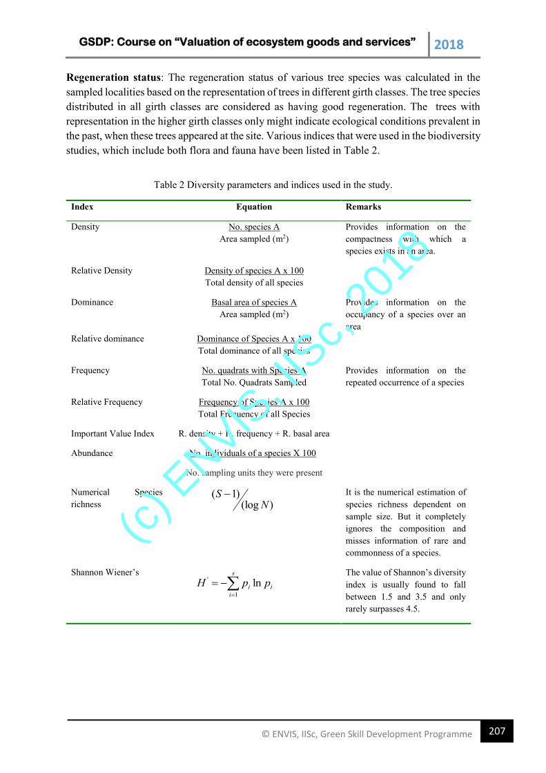
GSDP: Course on “Valuation of ecosystem goods and services” 2018
207 © ENVIS, IISc, Green Skill Development Programme
Regeneration status: The regeneration status of various tree species was calculated in the
sampled localities based on the representation of trees in different girth classes. The tree species
distributed in all girth classes are considered as having good regeneration. The trees with
representation in the higher girth classes only might indicate ecological conditions prevalent in
the past, when these trees appeared at the site. Various indices that were used in the biodiversity
studies, which include both flora and fauna have been listed in Table 2.
Table 2 Diversity parameters and indices used in the study.
Index Equation Remarks
Density No. species A
Area sampled (m2)
Provides information on the
compactness with which a
species exists in an area.
Relative Density Density of species A x 100
Total density of all species
Dominance Basal area of species A
Area sampled (m2)
Provides information on the
occupancy of a species over an
area
Relative dominance Dominance of Species A x 100
Total dominance of all species
Frequency No. quadrats with Species A
Total No. Quadrats Sampled
Provides information on the
repeated occurrence of a species
Relative Frequency Frequency of Species A x 100
Total Frequency of all Species
Important Value Index R. density + R. frequency + R. basal area
Abundance
No. individuals of a species X 100
No. sampling units they were present
Numerical Species
richness
It is the numerical estimation of
species richness dependent on
sample size. But it completely
ignores the composition and
misses information of rare and
commonness of a species.
Shannon Wiener’s The value of Shannon’s diversity
index is usually found to fall
between 1.5 and 3.5 and only
rarely surpasses 4.5.
)(log)1(
NS
s
i
ii ppH1
' ln
(c) E
NVIS, I
ISc,
2018
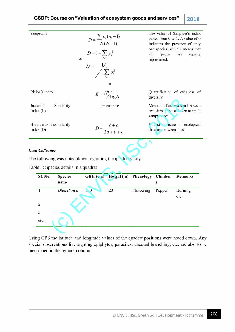
GSDP: Course on “Valuation of ecosystem goods and services” 2018
208 © ENVIS, IISc, Green Skill Development Programme
Simpson’s
or
or
The value of Simpson’s index
varies from 0 to 1. A value of 0
indicates the presence of only
one species, while 1 means that
all species are equally
represented.
Pielou’s index Quantification of evenness of
diversity.
Jaccard’s Similarity
Index (Ji)
Ji=a/a+b+c Measure of association between
two sites, unbiased even at small
sample sizes.
Bray-curtis dissimilarity
Index (D) cba
cbD
2
Robust measure of ecological
distance between sites.
Data Collection
The following was noted down regarding the quadrat study.
Table 3: Species details in a quadrat
Sl. No. Species
name
GBH (cm) Height (m) Phenology Climber
s
Remarks
1 Olea dioica 130 20 Flowering Pepper Burning
etc.
2
3
etc...
Using GPS the latitude and longitude values of the quadrat positions were noted down. Any
special observations like sighting epiphytes, parasites, unequal branching, etc. are also to be
mentioned in the remark column.
)1(
)1(
NN
nnD
ii
s
i
ip
D
1
2
1
s
i
ipD1
21
SHE
log'
(c) E
NVIS, I
ISc,
2018
GSDP: Course on “Valuation of ecosystem goods and services” 2018
209 © ENVIS, IISc, Green Skill Development Programme
11. Estimation of carbon sequestration by the terrestrial ecosystems
Forest ecosystems sequester atmospheric carbon and play a vital role in mitigating climate
change. Atmospheric carbon gets stored in the above and below ground biomass, dead organic
matter and soil organic matter. Mismanagement of forests leading to deforestation and
enhanced emissions during post industrial revolution has increased carbon dioxide
concentration in the atmosphere to 400 ppm from 270 ppm during the pre-industrial era. The
recent estimates of emissions in 30 developing countries (including Brazil, Bolivia, Indonesia,
Myanmar and Zambia) highlight that deforestation and forest degradation are the prime source
of CO2 imperilling productive ecosystems.
Figure 5 outlines the approach adopted for budgeting carbon in a district. The forest cover types
were identified using vegetation maps. Based on this, forest vegetation is sampled using
transect-based quadrats, which is validated and found appropriate especially in surveying
undulating forested landscapes of central Western Ghats. Topographic maps of 1:50000 scales
were used to do ground surveys and selection of sample plots. The analysis was carried out in
two major folds i.e., spatial mapping of carbon sinks, estimating carbon emissions.
Spatial mapping of carbon sinks
Field investigation: The study area is divided into 5’×5’ equal area grids covering approximately
81 km2 (9×9 km) and representative grids in each agro-climatic zone were chosen for further
investigations (Fig. 2). Field investigations are to be carried out in chosen grids through quadrat
based transects and compile data pertaining to the basal area, height, species, etc. Along a
transect of 180 m, 5 quadrats each of 20 m × 20 m are to be laid alternatively on the right and
left, for tree study (minimum girth of 30 cm at DBH (Diameter at Breast Height) or 130 cm
height from the ground), keeping intervals of 20 m length between successive quadrats. Within
each tree quadrat, at two diagonal corners, two sub-quadrats of 5 m × 5 m were laid for shrubs
and tree saplings (<30 cm girth). Within each of these 2 herb layer quadrats, 1 sq.m area each,
were also laid down for herbs and tree seedlings. Biomass is estimated from forests and also
plantations, to evaluate carbon sequestration potential of the respective ecosystem. Land use
analysis is performed to account grid wise forest cover, which helped further to estimate
biomass at the district level.
Quantification of biomass (Forests): The above ground standing biomass (AGB) of trees refers
to the cumulative weight of the tree biomass above ground, in a given area. The change in
standing biomass over a period of time is called productivity. Carbon storage in forests is
estimated by taking 50% of the biomass as carbon. AGB is a valuable measure for assessing
changes in forest structure and an essential aspect of studies of carbon cycle. AGB data at a
landscape scale can be used to understand changes in forest structure resulting from succession
or to differentiate between forest types. The AGB is calculated using the basal area (equation
1) and below ground biomass calculated from indirect estimation. The carbon storage is
computed by considering 50% of total biomass. The region specific allometric equations (Table
4) can be used to compute biomass. Probable relationship between basal area (BA), and forest
cover and extent of interior forest (equation 1) based on the field data coupled with land use
(c) E
NVIS, I
ISc,
2018

GSDP: Course on “Valuation of ecosystem goods and services” 2018
210 © ENVIS, IISc, Green Skill Development Programme
data. The multiple regression analysis is adopted, for estimating the relationship between a
dependent (standing biomass) and independent variables (forest cover, percentage of interior
forests-computed from land use analysis). The probable relationship helped in predicting the
standing biomass and carbon stock at the district level in all grids.
Fig. 5 Method adopted for carbon budgeting
𝐵𝑎𝑠𝑎𝑙 𝐴𝑟𝑒𝑎 (𝐵𝐴) = 𝐹{𝐼𝑛𝑡𝑒𝑟𝑖𝑜𝑟 𝑓𝑜𝑟𝑒𝑠𝑡, 𝑓𝑜𝑟𝑒𝑠𝑡 𝑐𝑜𝑣𝑒𝑟} ...1
Statistically, significant equations based on the basal area with land use and interior forest were obtained
and given in equations 2, 3, and 4 respectively for coastal, Sahyadri and plains. Validation of basal area
based on equation 2-4 was done with the known basal area in the respective grids. Later, basal area
(Table 5) for all grids in the respective agro-climatic zones are to be computed considering forest land
use and interior forests (in the respective grids) using equations 2, 3 and 4.
For Coastal regions,
BA = {30.1 +(0.0414 × (𝑓𝑜𝑟𝑒𝑠𝑡 𝑙𝑎𝑛𝑑 𝑢𝑠𝑒) + 0.053 × (𝑖𝑛𝑡𝑒𝑟𝑖𝑜𝑟 𝑓𝑜𝑟𝑒𝑠𝑡))};
𝑛 = 50, 𝑆𝐸 = 6.2 ...2
For Sahyadri Interior region,
BA = {39.1 +(−0.099 × (𝑓𝑜𝑟𝑒𝑠𝑡 𝑙𝑎𝑛𝑑 𝑢𝑠𝑒) + 0.091 × (𝑖𝑛𝑡𝑒𝑟𝑖𝑜𝑟 𝑓𝑜𝑟𝑒𝑠𝑡))};
𝑛 = 55, 𝑆𝐸 = 6.3 ...3
For plain region,
BA = {34.8 +(−0.186 × (𝑓𝑜𝑟𝑒𝑠𝑡 𝑙𝑎𝑛𝑑 𝑢𝑠𝑒) + 0.12 × (𝑖𝑛𝑡𝑒𝑟𝑖𝑜𝑟 𝑓𝑜𝑟𝑒𝑠𝑡))};
𝑛 = 11, 𝑆𝐸 = 5.5 . ...4
Where n is a number of transects and SE refers to standard error.
(c) E
NVIS, I
ISc,
2018
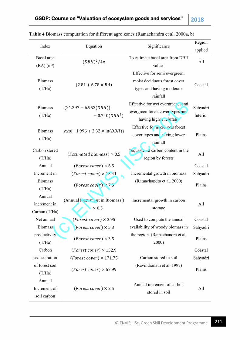
GSDP: Course on “Valuation of ecosystem goods and services” 2018
211 © ENVIS, IISc, Green Skill Development Programme
Table 4 Biomass computation for different agro zones (Ramachandra et al. 2000a, b)
Index Equation Significance Region
applied
Basal area
(BA) (m²) (𝐷𝐵𝐻)2 4𝜋⁄
To estimate basal area from DBH
values All
Biomass
(T/Ha) (2.81 + 6.78 × 𝐵𝐴)
Effective for semi evergreen,
moist deciduous forest cover
types and having moderate
rainfall
Coastal
Biomass
(T/Ha)
(21.297 − 6.953(𝐷𝐵𝐻))
+ 0.740(𝐷𝐵𝐻2)
Effective for wet evergreen, semi
evergreen forest cover types and
having higher rainfall)
Sahyadri
Interior
Biomass
(T/Ha)
𝑒𝑥𝑝{−1.996 + 2.32 × ln(𝐷𝐵𝐻)}
Effective for deciduous forest
cover types and having lower
rainfall
Plains
Carbon stored
(T/Ha) (𝐸𝑠𝑡𝑖𝑚𝑎𝑡𝑒𝑑 𝑏𝑖𝑜𝑚𝑎𝑠𝑠) × 0.5
Sequestered carbon content in the
region by forests All
Annual
Increment in
Biomass
(T/Ha)
(𝐹𝑜𝑟𝑒𝑠𝑡 𝑐𝑜𝑣𝑒𝑟) × 6.5
Incremental growth in biomass
(Ramachandra et al. 2000)
Coastal
(𝐹𝑜𝑟𝑒𝑠𝑡 𝑐𝑜𝑣𝑒𝑟) × 13.41 Sahyadri
(𝐹𝑜𝑟𝑒𝑠𝑡 𝑐𝑜𝑣𝑒𝑟) × 7.5 Plains
Annual
increment in
Carbon (T/Ha)
(Annual Increment in Biomass )
× 0.5
Incremental growth in carbon
storage All
Net annual
Biomass
productivity
(T/Ha)
(𝐹𝑜𝑟𝑒𝑠𝑡 𝑐𝑜𝑣𝑒𝑟) × 3.95 Used to compute the annual
availability of woody biomass in
the region. (Ramachandra et al.
2000)
Coastal
(𝐹𝑜𝑟𝑒𝑠𝑡 𝑐𝑜𝑣𝑒𝑟) × 5.3 Sahyadri
(𝐹𝑜𝑟𝑒𝑠𝑡 𝑐𝑜𝑣𝑒𝑟) × 3.5 Plains
Carbon
sequestration
of forest soil
(T/Ha)
(𝐹𝑜𝑟𝑒𝑠𝑡 𝑐𝑜𝑣𝑒𝑟) × 152.9
Carbon stored in soil
(Ravindranath et al. 1997)
Coastal
(𝐹𝑜𝑟𝑒𝑠𝑡 𝑐𝑜𝑣𝑒𝑟) × 171.75 Sahyadri
(𝐹𝑜𝑟𝑒𝑠𝑡 𝑐𝑜𝑣𝑒𝑟) × 57.99 Plains
Annual
Increment of
soil carbon
(𝐹𝑜𝑟𝑒𝑠𝑡 𝑐𝑜𝑣𝑒𝑟) × 2.5 Annual increment of carbon
stored in soil All
(c) E
NVIS, I
ISc,
2018
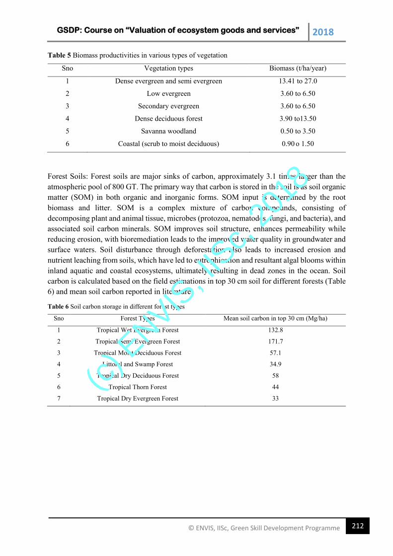
GSDP: Course on “Valuation of ecosystem goods and services” 2018
212 © ENVIS, IISc, Green Skill Development Programme
Table 5 Biomass productivities in various types of vegetation
Sno Vegetation types Biomass (t/ha/year)
1 Dense evergreen and semi evergreen 13.41 to 27.0
2 Low evergreen 3.60 to 6.50
3 Secondary evergreen 3.60 to 6.50
4 Dense deciduous forest 3.90 to13.50
5 Savanna woodland 0.50 to 3.50
6 Coastal (scrub to moist deciduous) 0.90 o 1.50
Forest Soils: Forest soils are major sinks of carbon, approximately 3.1 times larger than the
atmospheric pool of 800 GT. The primary way that carbon is stored in the soil is as soil organic
matter (SOM) in both organic and inorganic forms. SOM input is determined by the root
biomass and litter. SOM is a complex mixture of carbon compounds, consisting of
decomposing plant and animal tissue, microbes (protozoa, nematodes, fungi, and bacteria), and
associated soil carbon minerals. SOM improves soil structure, enhances permeability while
reducing erosion, with bioremediation leads to the improved water quality in groundwater and
surface waters. Soil disturbance through deforestation also leads to increased erosion and
nutrient leaching from soils, which have led to eutrophication and resultant algal blooms within
inland aquatic and coastal ecosystems, ultimately resulting in dead zones in the ocean. Soil
carbon is calculated based on the field estimations in top 30 cm soil for different forests (Table
6) and mean soil carbon reported in literature.
Table 6 Soil carbon storage in different forest types
Sno Forest Types Mean soil carbon in top 30 cm (Mg/ha)
1 Tropical Wet Evergreen Forest 132.8
2 Tropical Semi Evergreen Forest 171.7
3 Tropical Moist Deciduous Forest 57.1
4 Littoral and Swamp Forest 34.9
5 Tropical Dry Deciduous Forest 58
6 Tropical Thorn Forest 44
7 Tropical Dry Evergreen Forest 33
(c) E
NVIS, I
ISc,
2018
GSDP: Course on “Valuation of ecosystem goods and services” 2018
213 © ENVIS, IISc, Green Skill Development Programme
12. Forest Ecosystem – Goods and services
Ramachandra T. V., Divya Soman, Ashwath D. Naik and M. D. Subash Chandran, 2017. Appraisal of
Forest Ecosystems Goods and Services: Challenges and Opportunities for Conservation, Journal of
Biodiversity, 8(1): 12-33 (2017), DOI: http://10.1080/09766901.2017.1346160
FAO (2000) has defined forest as an area with an expected tree canopy of more than 10%; and
a total area of more 0.5 hectares where trees reach at least 5 meters in size. Among the terrestrial
biomes, forests occupy about 31 % (4,033 million hectare) of the world’s total land area and
of which 93% of the world’s forest cover is natural forest and 7% is planted (FAO, 2010;
TEEB, 2010). Forest ecosystems account for over two-thirds of net primary production on
land–the conversion of solar energy into biomass through photosynthesis making them a key
component of the global carbon cycle and climate (MEA, 2005). Forest can be defined as a
terrestrial unit of living organisms (plants, animals and microorganisms), interacting among
themselves and with the environment (soil, climate, water and light) in which they live. Forest
ecosystem services can provide both direct and indirect economic benefits. The forests of the
world harbor very large and complex biological species diversity and hence, it becomes a
complex thing to assign a specific definition or explanation for it. The species diversity is an
indicator for biological diversity and the species richness increases as we move from the poles
to the equatorial region.
India’s forest has been classified into four major groups, namely, tropical, sub-tropical,
temperate, and alpine (Champion and Seth, 1968). These major groups are further divided into
16 type groups: Tropical (wet evergreen, semi-evergreen, moist deciduous, littoral and swamp,
dry deciduous, thorn, dry evergreen), Sub-tropical (broad leaved hill forests, pine, and dry
evergreen), Temperate (montane wet, Himalayan moist temperate, Himalayan dry temperate),
and Alpine (sub-alpine, moist alpine and dry alpine scrub). Tropical forest in particular
contributes more than the other terrestrial biomes to climate relevant cycles and biodiversity
related processes (Pearce and Pearce, 2001). These forests constitute the earth’s major genetic
reservoir and global water cycles (Anderson and Bojo, 1992). They represent a huge economic
asset for the region where they occur.
13. Ecosystem Goods and Services
The ecosystem provides various fundamental benefits for our survival such as food; soil
production, erosion and control; climate regulation; water purification; bioenergy, etc. These
benefits and services are referred to as ‘Ecosystem services’ and are very crucial for the
survival of humans and other organisms on the earth. The ecosystems, if in a good condition
perform functions which are of bio-geophysical in nature. These functions result in the flow of
various services and benefits for humans and their society (Kumar and Kumar, 2008).
Ecosystem Functions can be defined as ‘the capacity of natural processes and components to
provide goods and services that satisfy human needs, directly or indirectly’ (De Groot et al.,
2002). MEA (2005) defines ecosystem services as the benefits people obtain from ecosystems.
It includes provisioning services such as food and water, regulating services such as flood and
(c) E
NVIS, I
ISc,
2018
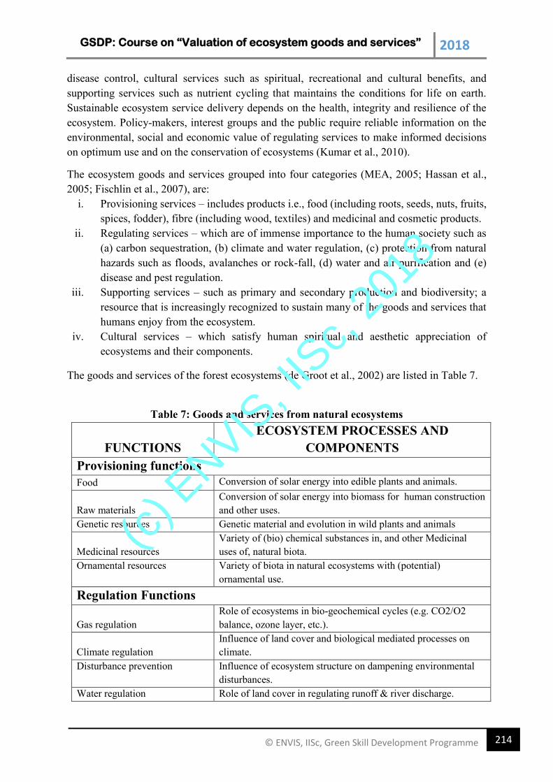
GSDP: Course on “Valuation of ecosystem goods and services” 2018
214 © ENVIS, IISc, Green Skill Development Programme
disease control, cultural services such as spiritual, recreational and cultural benefits, and
supporting services such as nutrient cycling that maintains the conditions for life on earth.
Sustainable ecosystem service delivery depends on the health, integrity and resilience of the
ecosystem. Policy-makers, interest groups and the public require reliable information on the
environmental, social and economic value of regulating services to make informed decisions
on optimum use and on the conservation of ecosystems (Kumar et al., 2010).
The ecosystem goods and services grouped into four categories (MEA, 2005; Hassan et al.,
2005; Fischlin et al., 2007), are:
i. Provisioning services – includes products i.e., food (including roots, seeds, nuts, fruits,
spices, fodder), fibre (including wood, textiles) and medicinal and cosmetic products.
ii. Regulating services – which are of immense importance to the human society such as
(a) carbon sequestration, (b) climate and water regulation, (c) protection from natural
hazards such as floods, avalanches or rock-fall, (d) water and air purification and (e)
disease and pest regulation.
iii. Supporting services – such as primary and secondary production and biodiversity; a
resource that is increasingly recognized to sustain many of the goods and services that
humans enjoy from the ecosystem.
iv. Cultural services – which satisfy human spiritual and aesthetic appreciation of
ecosystems and their components.
The goods and services of the forest ecosystems (de Groot et al., 2002) are listed in Table 7.
Table 7: Goods and services from natural ecosystems
FUNCTIONS
ECOSYSTEM PROCESSES AND
COMPONENTS
Provisioning functions
Food Conversion of solar energy into edible plants and animals.
Raw materials
Conversion of solar energy into biomass for human construction
and other uses.
Genetic resources Genetic material and evolution in wild plants and animals
Medicinal resources
Variety of (bio) chemical substances in, and other Medicinal
uses of, natural biota.
Ornamental resources Variety of biota in natural ecosystems with (potential)
ornamental use.
Regulation Functions
Gas regulation
Role of ecosystems in bio-geochemical cycles (e.g. CO2/O2
balance, ozone layer, etc.).
Climate regulation
Influence of land cover and biological mediated processes on
climate.
Disturbance prevention Influence of ecosystem structure on dampening environmental
disturbances.
Water regulation Role of land cover in regulating runoff & river discharge.
(c) E
NVIS, I
ISc,
2018
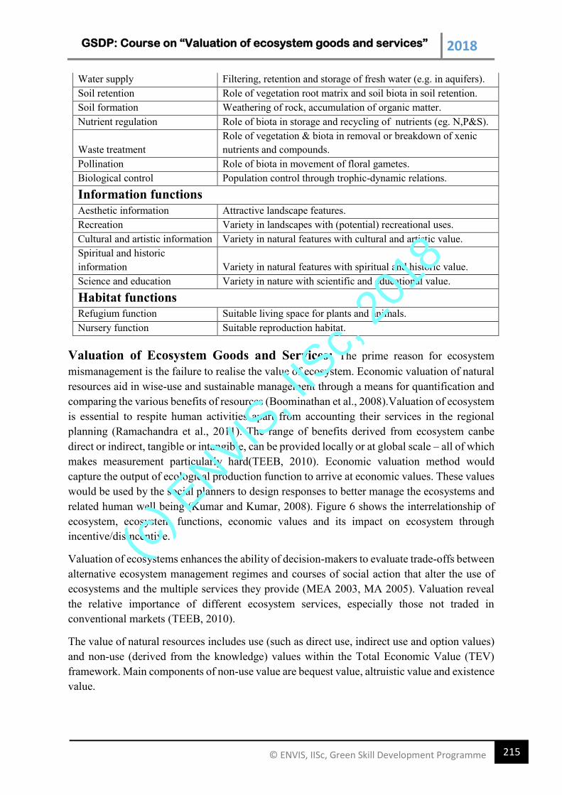
GSDP: Course on “Valuation of ecosystem goods and services” 2018
215 © ENVIS, IISc, Green Skill Development Programme
Water supply Filtering, retention and storage of fresh water (e.g. in aquifers).
Soil retention Role of vegetation root matrix and soil biota in soil retention.
Soil formation Weathering of rock, accumulation of organic matter.
Nutrient regulation Role of biota in storage and recycling of nutrients (eg. N,P&S).
Waste treatment
Role of vegetation & biota in removal or breakdown of xenic
nutrients and compounds.
Pollination Role of biota in movement of floral gametes.
Biological control Population control through trophic-dynamic relations.
Information functions
Aesthetic information Attractive landscape features.
Recreation Variety in landscapes with (potential) recreational uses.
Cultural and artistic information Variety in natural features with cultural and artistic value.
Spiritual and historic
information Variety in natural features with spiritual and historic value.
Science and education Variety in nature with scientific and educational value.
Habitat functions
Refugium function Suitable living space for plants and animals.
Nursery function Suitable reproduction habitat.
Valuation of Ecosystem Goods and Services: The prime reason for ecosystem
mismanagement is the failure to realise the value of ecosystem. Economic valuation of natural
resources aid in wise-use and sustainable management through a means for quantification and
comparing the various benefits of resources (Boominathan et al., 2008).Valuation of ecosystem
is essential to respite human activities apart from accounting their services in the regional
planning (Ramachandra et al., 2011). The range of benefits derived from ecosystem canbe
direct or indirect, tangible or intangible, can be provided locally or at global scale – all of which
makes measurement particularly hard(TEEB, 2010). Economic valuation method would
capture the output of ecological production function to arrive at economic values. These values
would be used by the social planners to design responses to better manage the ecosystems and
related human well being (Kumar and Kumar, 2008). Figure 6 shows the interrelationship of
ecosystem, ecosystem functions, economic values and its impact on ecosystem through
incentive/disincentive.
Valuation of ecosystems enhances the ability of decision-makers to evaluate trade-offs between
alternative ecosystem management regimes and courses of social action that alter the use of
ecosystems and the multiple services they provide (MEA 2003, MA 2005). Valuation reveal
the relative importance of different ecosystem services, especially those not traded in
conventional markets (TEEB, 2010).
The value of natural resources includes use (such as direct use, indirect use and option values)
and non-use (derived from the knowledge) values within the Total Economic Value (TEV)
framework. Main components of non-use value are bequest value, altruistic value and existence
value.
(c) E
NVIS, I
ISc,
2018
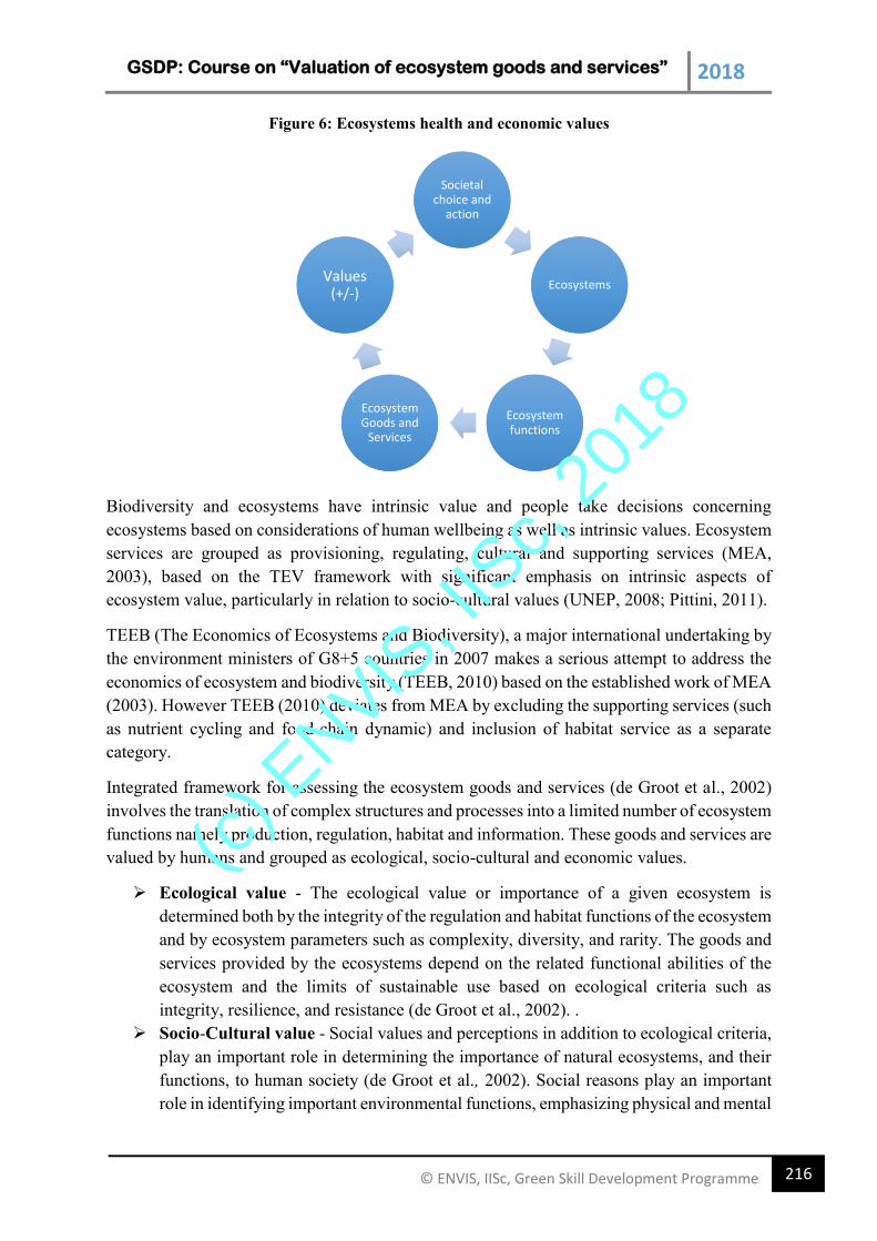
GSDP: Course on “Valuation of ecosystem goods and services” 2018
216 © ENVIS, IISc, Green Skill Development Programme
Figure 6: Ecosystems health and economic values
Biodiversity and ecosystems have intrinsic value and people take decisions concerning
ecosystems based on considerations of human wellbeing as well as intrinsic values. Ecosystem
services are grouped as provisioning, regulating, cultural and supporting services (MEA,
2003), based on the TEV framework with significant emphasis on intrinsic aspects of
ecosystem value, particularly in relation to socio-cultural values (UNEP, 2008; Pittini, 2011).
TEEB (The Economics of Ecosystems and Biodiversity), a major international undertaking by
the environment ministers of G8+5 countries in 2007 makes a serious attempt to address the
economics of ecosystem and biodiversity (TEEB, 2010) based on the established work of MEA
(2003). However TEEB (2010) deviates from MEA by excluding the supporting services (such
as nutrient cycling and food-chain dynamic) and inclusion of habitat service as a separate
category.
Integrated framework for assessing the ecosystem goods and services (de Groot et al., 2002)
involves the translation of complex structures and processes into a limited number of ecosystem
functions namely production, regulation, habitat and information. These goods and services are
valued by humans and grouped as ecological, socio-cultural and economic values.
Ecological value - The ecological value or importance of a given ecosystem is
determined both by the integrity of the regulation and habitat functions of the ecosystem
and by ecosystem parameters such as complexity, diversity, and rarity. The goods and
services provided by the ecosystems depend on the related functional abilities of the
ecosystem and the limits of sustainable use based on ecological criteria such as
integrity, resilience, and resistance (de Groot et al., 2002). .
Socio-Cultural value - Social values and perceptions in addition to ecological criteria,
play an important role in determining the importance of natural ecosystems, and their
functions, to human society (de Groot et al., 2002). Social reasons play an important
role in identifying important environmental functions, emphasizing physical and mental
Societal choice and
action
Societal choice and
action
EcosystemsEcosystems
Ecosystem functions
Ecosystem functions
Ecosystem Goods and
Services
Ecosystem Goods and
Services
Values (+/-)
Values (+/-)
(c) E
NVIS, I
ISc,
2018
GSDP: Course on “Valuation of ecosystem goods and services” 2018
217 © ENVIS, IISc, Green Skill Development Programme
health, education, cultural diversity and identity (heritage value), freedom and spiritual
values.
Economic value - Economic value is the value that a person is willing to give up in
order to obtain goods, service, or state of the world. A person’s willingness to pay states
the economic preferences attached to the particular environmental benefit.Thus their
willingness to pay reflects the economic value (Ramachandra et al., 2005). Economic
value establishes a common metric of value (money). All values are estimated using
the common metric, which helps in aggregating values of different goods and services
(DEFRA, 2007). When the market does not capture the value of environmental goods
or services, techniques associated with ‘shadow pricing’ or ‘proxy price’ are used to
indirectly estimate its value.
Estimation of the economic values for 17 different ecosystem services for 16 different biomes
based on earlier published studies and some original calculations (Costanza et al., 1997)
highlight that the annual value of the ecosystem services of the terrestrial and aquatic biomes
of the world is in the range of USD 16–54 trillion with an estimated average of USD 33 trillion.
This value was found to be 1.8 times higher than the global gross national product (GNP).
About 63% of the estimated values of ecosystem services were found to be contributed by the
marine ecosystems while about 38% of the estimated values were found to be contributed by
the terrestrial ecosystems, mainly from the forests and wetlands.
Forest Ecosystem Services
Forest ecosystem services, like services from other ecosystem, have great economic value
(Costanza et al., 1997; Pearce and Pearce 2001; Pearce et al., 2002). Forests worldwide are
known to be critically important habitats in terms of the biological diversity they contain and
in terms of the ecological functions they serve. Forests, particularly tropical forests, contribute
more than other terrestrial biomes to climate relevant cycles and processes and also to
biodiversity related processes (Nasi et al., 2002). Forest ecosystem services, as with other
nature’s services, have also been claimed to be of great economic value (Costanza et al., 1997;
Pearce and Pearce 2001; Pearce and Moran 1994). These ecosystems are extremely important
refuges for terrestrial biodiversity, serve as a central component of Earth’s biogeochemical
systems and are a source of ecosystem services essential for human well-being (Gonzalez et
al., 2005).
The forest ecosystem provides a large number of valuable products such as timber, firewood,
non-timber forest product, biodiversity, genetic resources, medicinal plants, etc. The forest
trees are felled on a large scale for using their wood as timber and firewood. There are two
types of needs for timber: commercial and industrial. The commercial timber production is the
local utilization of timber while the industrial timber is used by the industries. According to
FAO (2010), wood removals valued just over US$100 billion annually in the period 2003–
2007, mainly accounted for by industrial round wood. Further, 11% of world energy
consumption comes from biomass, mainly fuel wood (CBD, 2001). 19% of China's primary
energy consumption comes from biomass, the figure for India being 42%, and the figure for
developing countries generally being about 35% (IEA 1998; UNDP 2000). Non-commercial
(c) E
NVIS, I
ISc,
2018
GSDP: Course on “Valuation of ecosystem goods and services” 2018
218 © ENVIS, IISc, Green Skill Development Programme
sources of energy (such as fire wood, agriculturaland horticultural residues, and animal
residues) contribute about 54% of the total energy in Karnataka.
Timber and carbon wealth assessment in the forests of India (Atkinson and Gundimeda, 2006)
show the opening stock of forest resources as 4,740,858,000 cubic meters and about 639,600
sq. km of forest area at the beginning of 1993-94. Biomass density/ha in Indian forests is about
92 t/ha and carbon values of Indian forests is 2933.8 million tones assessed considering a
carbon content of 0.5 Mg C per Mg oven dry biomass (Haripriya, 2002). The closing stock of
the timber is 4704 million cum and the estimate of value is Rs. 9454 billion, the stock of the
carbon is 2872 million tons with a value estimate of Rs.1811 billion.
Apart from serving as a storehouse of wood which is used for various purposes, there are also
equally important non-wood products that are obtained from the forests. The botanical and
other natural products, other than timber extracted from the forest system are referred to as
non-timber forest products (NTFPs). These resources/products have been extracted from the
forest ecosystems and are being utilised within the household or marketed or have social,
cultural or religious significance (FAO, 1990). NTFP is a significant component due to its
important bearing on rural livelihoods and subsistence. NTFPs are also referred ‘minor forest
produce’ as most of NTFP are consumed by local populations, and are not marketed (Arnold
and Pérez, 2001). These include plants and plant materials used for food, fuel, storage and
fodder, medicine, cottage and wrapping materials, biochemical, animals, birds, reptiles and
fishes, for food and feather. Unlike timber-based products, these products come from variety
of sources like: fruits and vegetables to eat, leaves and twigs for decoration, flowers for various
purposes, herbal medicines from different plant parts, wood carvings and decorations, etc. The
values of NTFPs are of critical importance as source of income and employment for rural
people living around the forest regions, especially during lean seasons of agricultural crops.
NTFPs provide 40-63% of the total annual income of the people residing in rural areas of
Madhya Pradesh (Tewari and Campbell, 1996) and accounted 20-35% of the household
incomes in West Bengal. Similarly wild plant resources contributed US$ 194 – 1114per
household per year in seven study areas in southern African region (Shackleton et al., 2000).
The net present value (NPV) of the forest for sustainable fruit and latex production is estimated
at US$6,330/ha considering the net revenue from a single year’s harvest of fruit and latex
production as US$422/ha in Mishana, Rio Nanay, Peru (Peters et al., 1989) on the assumption
of availability in perpetuity, constant real prices and a discount rate of 5%.
Evaluation of the direct use benefits to rural communities’ from harvesting NTFPs and using
forest areas for agriculture and residential space, near the Mantadia National Park, in
Madagascar (Kramer et al., 1992; 1995)through contingency valuation (CV) show an aggregate
net present value for the affected population (about 3,400 people) of US$673,000 with an
annual mean value per household of USD 108.
Estimation of the quantity of the NTFPs collected by the locals and forest department based on
a questionnaire based survey in 21 villages of four different forest zones in Uttara Kannada
district (Murthy et al., 2005), indicate the collection of 59 different plant species in the
evergreen forests, 40 different plant species in the semi-evergreen forests, 12 different plant
(c) E
NVIS, I
ISc,
2018
GSDP: Course on “Valuation of ecosystem goods and services” 2018
219 © ENVIS, IISc, Green Skill Development Programme
species in moist deciduous and 15 different plant species in dry deciduous forests and about
42–80 NTFP species of medicinal importance are marketed in herbal shops. Valuation reveal
an annual income per household ranges from Rs. 3,445 (evergreen forests), 3,080 (moist
deciduous), 1,438 (semi-evergreen) to Rs. 1,233 (dry deciduous).
Assessment of the marketing potential of different value added products from Artocarpus sps.
in Uttara Kannada district based on field surveys and the discussions with the local people and
industries (Ramana and Patil, 2008), revealed that Artocarpus integrifolia collected from
nearby forest area and home gardens is most extensively used for preparing items like chips,
papad, sweets, etc. Chips and papads are commercially produced and sold in the markets, and
primary collectors get 25% and the processing industry get 50% of of the total amount paid by
the consumers.
Forest ecosystems also provide other indirect benefits like ground water recharge, soil
retention, gas regulation, waste treatment, pollination, refugium function, nursery function etc.
in addition to the direct benefits (De Groot et al., 2002). Forest vegetation aids in the
percolation and recharging of groundwater sources while allowing moderate run off. Gas
regulation functions include general maintenance of habits through the maintenance of clean
air, prevention of diseases (e.g. skin cancer), etc.
Forests act as carbon sinks by taking carbon during photosynthesis and synthesis of organic
compounds, which aids in maintaining CO2/O 2 balance, ozone layer and also sulphur dioxide
balance. Carbon sequestration potential of 131t of carbon per hectare with the above ground
biomass of 349 ton/ha has been estimated in the relic forest of Uttara Kannada (Chandran et
al., 2010) and 11.8 Metric ton (1995) in forests in India with the carbon uptake potential of
55.48 Mt (2020) and 73.48 Mt (2045) respectively (Lal and Singh, 2000) projected the total
carbon uptake for the year 2020 and 2045 and the value was found to be. The carbon
sequestration potential was found to be 4.1 and 9.8 Gt by 2020 and 2045 respectively.
Vegetative structure of forests through its storage capacity and surface resistance plays a vital
role in the disturbance regulation by altering potentially catastrophic effects of storms, floods
and droughts. Soil retention occurs by the presence of the vegetation cover which holds the soil
and prevents the loss of top soil. Pollination is an important ecological service provided by the
forest ecosystem and the studies have revealed of forest dwelling pollinators (such as bees)
make significant contribution to the agricultural production of a broad range of crops, in
particular fruits, vegetables, fiber crops and nuts (Costanza et al., 1997).
Forest also helps in aesthetic benefit, recreational benefit, science and education, spiritual
benefits, etc. The scenic beauty of forests provides aesthetic and recreational benefits through
psychological relief to the visitors. An investigation of cultural services of the forest of
Uttaranchal (Djafar, 2006) considering six services namely aesthetic, recreational, cultural
heritage and identity, inspirational, spiritual and religious and educational function, highlight
the recreational value of forests US$ 0.82/ha/yr for villager’s per visit. Aesthetic value derived
by the preference of the villagers was estimated as US$ 7-1760 /ha/yr derived by the preference
of the villagers to live in the sites where there is good scenery. Cultural heritage and identity
value was estimated as USD 1-25/ha/yr based on 24 places, 43 plant species and 16 animal
(c) E
NVIS, I
ISc,
2018
GSDP: Course on “Valuation of ecosystem goods and services” 2018
220 © ENVIS, IISc, Green Skill Development Programme
species. Spiritual and religious areas was about USD 1-25/ha/yr. Educational value was
obtained from the research activity and value was similar to spiritual and religious values.
Ecotourism benefit of the domestic visitor using the travel cost method in the Periyar tiger
reserve in Kerala is Rs. 161.3 per visitor (Manoharan et al. 1999), with average consumer
surplus at Rs. 9.89 per domestic visitor and Rs. 140 for foreign tourists. The value of eco-
tourism (as per 2005) is extrapolated as Rs. 84.5 million. The recreational value assessment of
Vazhachal and Athirappily of Kerala (Anitha and Muraleedharan, 2006) reveal that visitor flow
on an average is 2.3 lakh (at Vazhachal) and 5.3 lakh (Athirappily) visitors/year and the average
fee collection ranges from Rs. 10 (Vazhachal) to Rs.23.5 (Athirappily) lakh / year at. Parking
fee for vehicles itself is about Rs. 1.39 (Vazhachal) lakh /year and Rs. 2.7 (Athirappily) lakh/
year. About Rs. 5.6 lakh is earned from visitors entrance fee and parking charges. The
estimated aggregate recreation surplus of the sample is equal to Rs 20, 69,214 with an average
recreation surplus per visitor of Rs. 2,593.
Recreational value in the protected site of Western Ghats (Mohandas and Remadevi, 2011)
based on the relationship between travel cost and visitation rate and the willingness to pay is
Rs. 26.7 per visitor and the average consumer surplus per visit is Rs. 290. A similar study
carried out in the valley of a national park show the net recreational benefit as Rs.5,88,332 and
the average consumer surplus as Rs 194.68 (Gera et al., 2008). The total recreation value of
Dandeli wildlife sanctuary using travel cost method during 2004-05 show the total recreation
value of Rs. 37,142.86 per Sq. kmwith the total value of Rs. 1,76,43,600 (Panchamukhi et al.,
2007). Similarly, based on the willingness to pay for the preservation of watershed in Karnataka
estimate show a value of Rs.125.45per hectare and the total value of Rs. 480 million (for 2004-
05).
Valuation of forest in Uttarakhand, Himalayas using the benefit transfer method (Madhu
Verma, 2007) shows a value of Uttarkhand forests as Rs. 16,192 billion accounting Rs. 19,035
million from the direct benefits (including tourism) and Rs. are the indirect benefits as173,120
million and silt control service is accounted as Rs. 2062.2 million. Carbon sequestration is
accounted as Rs.2974/million at US $ 10 per t of C considering the net accumulation of 6.6 Mt
C per year in biomass. Aesthetic beauty of the landscape is estimated as 10,665.3 million and
pollination service value is accounted to be Rs. 25,610 million/yr. Natural ecosystems also
provide unlimited opportunities for environmental education and function as field laboratories
for scientific research (De Groot et al., 2002).
Sacred groves present in varied ecosystems viz., evergreen and deciduous forests, hill tops,
valleys, mangroves, swamps and even in agricultural fields in Uttara Kannada district represent
varied vegetation and animal profiles (Ray et al., 2011).The protection of patches of forest as
sacred groves and of several tree species as sacred trees leads to the spiritual function provided
by the forest (Chandran, 1993). Sacred groves also play an important role in the cultural service
provided by the forest. The groves do not fetch any produce which can be used for direct
consumptive or commercial purpose. Creation of hypothetical market fetches price worth Rs.
600/quintal for a woody species and Rs. 40/quintal for non wood product. The value of sacred
(c) E
NVIS, I
ISc,
2018
GSDP: Course on “Valuation of ecosystem goods and services” 2018
221 © ENVIS, IISc, Green Skill Development Programme
grove assessed through willingness to pay to preserve the sacred grove in Siddapur taluk of
Uttara Kannada district (Panchamukhi et al. 2008), show the value Rs. 7280/per hectare.
The major threat to the forests today is deforestation caused by several reasons such as rise in
the population, exploitation activities which include expansion of agriculture land, ranching,
wood extraction, development of infrastructure. Shifting cultivation is considered to be one of
the most important causes of deforestation (Myers, 1984). The loss of biodiversity is the second
most important problem in nearly every terrestrial ecosystem on Earth. This loss is accelerating
driven by the over-exploitation of natural resources, habitat destruction, fragmentation and
climate change (MEA, 2003). Even though the Convention on Biological Diversity (CBD) has
adopted a target of reducing the rate of biodiversity loss at global, regional and national levels
by 2010 (Mace, 2005; Fontaine et al., 2007), still the loss of biodiversity is at a high pace.
Nearly 75% of the genetic diversity of domesticated crop plants has been lost in the past century
(WEHAB, 2002),.About 24% of mammals and 12% of bird species are currently considered to
be globally threatened. Despite the essential functions of ecosystems and the consequences of
their degradation, ecosystem services are undervalued by society, because of the lack of
awareness of the link between natural ecosystems and the functioning of human support
systems.
METHOD – Valuation of Ecosystem Goods and Services
The framework for incorporating the true value of forest in the GDP requires thorough
valuation of the benefits derived from forest ecosystems. Taluk wise forest valuation has been
done through the quantification of goods, estimation of values based on the market price, and
compilation of values of ecosystem services form literatures. Total economic value of the
forest ecosystems in Uttara Kannada has been done (which is discussed in the following
sections) considering i) provisioning services, ii) regulating services, iii) supporting services
and iv) information services (MEA 2003). Various components of provisioning, regulating,
cultural and supporting services are listed in Figure 7. The research includes compilation of
data from primary (field investigations) and secondary sources (government agencies,
published scientific literatures in peer reviewed journals). Data on quantity of timber and non
– timber forest products harvested were collected from Divisional Office (Sirsi) of Karnataka
Forest Department, Government of Karnataka. Data on the prices of various marketed forest
products were collected through market survey. Data on various other provisioning goods and
services were compiled from literature pertaining to ecological and socio-economic studies in
the district and also through interview with the subject experts.
(c) E
NVIS, I
ISc,
2018
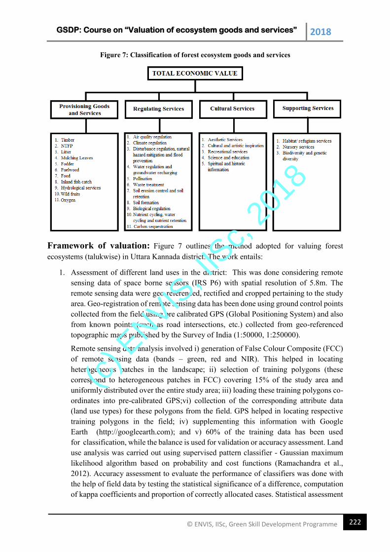
GSDP: Course on “Valuation of ecosystem goods and services” 2018
222 © ENVIS, IISc, Green Skill Development Programme
Figure 7: Classification of forest ecosystem goods and services
Framework of valuation: Figure 7 outlines the method adopted for valuing forest
ecosystems (talukwise) in Uttara Kannada district. The work entails:
1. Assessment of different land uses in the district: This was done considering remote
sensing data of space borne sensors (IRS P6) with spatial resolution of 5.8m. The
remote sensing data were geo-referenced, rectified and cropped pertaining to the study
area. Geo-registration of remote sensing data has been done using ground control points
collected from the field using pre calibrated GPS (Global Positioning System) and also
from known points (such as road intersections, etc.) collected from geo-referenced
topographic maps published by the Survey of India (1:50000, 1:250000).
Remote sensing data analysis involved i) generation of False Colour Composite (FCC)
of remote sensing data (bands – green, red and NIR). This helped in locating
heterogeneous patches in the landscape; ii) selection of training polygons (these
correspond to heterogeneous patches in FCC) covering 15% of the study area and
uniformly distributed over the entire study area; iii) loading these training polygons co-
ordinates into pre-calibrated GPS;vi) collection of the corresponding attribute data
(land use types) for these polygons from the field. GPS helped in locating respective
training polygons in the field; iv) supplementing this information with Google
Earth (http://googleearth.com); and v) 60% of the training data has been used
for classification, while the balance is used for validation or accuracy assessment. Land
use analysis was carried out using supervised pattern classifier - Gaussian maximum
likelihood algorithm based on probability and cost functions (Ramachandra et al.,
2012). Accuracy assessment to evaluate the performance of classifiers was done with
the help of field data by testing the statistical significance of a difference, computation
of kappa coefficients and proportion of correctly allocated cases. Statistical assessment
(c) E
NVIS, I
ISc,
2018
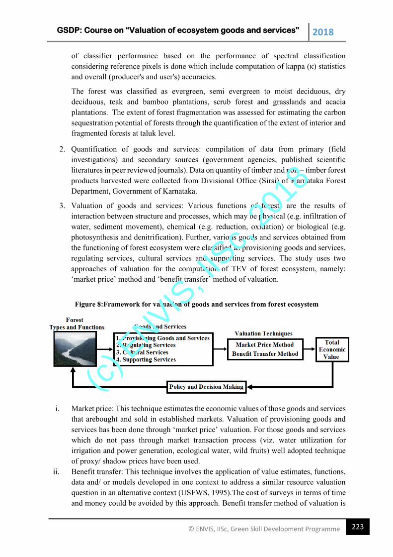
GSDP: Course on “Valuation of ecosystem goods and services” 2018
223 © ENVIS, IISc, Green Skill Development Programme
of classifier performance based on the performance of spectral classification
considering reference pixels is done which include computation of kappa (κ) statistics
and overall (producer's and user's) accuracies.
The forest was classified as evergreen, semi evergreen to moist deciduous, dry
deciduous, teak and bamboo plantations, scrub forest and grasslands and acacia
plantations. The extent of forest fragmentation was assessed for estimating the carbon
sequestration potential of forests through the quantification of the extent of interior and
fragmented forests at taluk level.
2. Quantification of goods and services: compilation of data from primary (field
investigations) and secondary sources (government agencies, published scientific
literatures in peer reviewed journals). Data on quantity of timber and non – timber forest
products harvested were collected from Divisional Office (Sirsi) of Karnataka Forest
Department, Government of Karnataka.
3. Valuation of goods and services: Various functions of forests are the results of
interaction between structure and processes, which may be physical (e.g. infiltration of
water, sediment movement), chemical (e.g. reduction, oxidation) or biological (e.g.
photosynthesis and denitrification). Further, various goods and services obtained from
the functioning of forest ecosystem were classified as provisioning goods and services,
regulating services, cultural services and supporting services. The study uses two
approaches of valuation for the computation of TEV of forest ecosystem, namely:
‘market price’ method and ‘benefit transfer’ method of valuation.
Figure 8:Framework for valuation of goods and services from forest ecosystem
i. Market price: This technique estimates the economic values of those goods and services
that arebought and sold in established markets. Valuation of provisioning goods and
services has been done through ‘market price’ valuation. For those goods and services
which do not pass through market transaction process (viz. water utilization for
irrigation and power generation, ecological water, wild fruits) well adopted technique
of proxy/ shadow prices have been used.
ii. Benefit transfer: This technique involves the application of value estimates, functions,
data and/ or models developed in one context to address a similar resource valuation
question in an alternative context (USFWS, 1995).The cost of surveys in terms of time
and money could be avoided by this approach. Benefit transfer method of valuation is
(c) E
NVIS, I
ISc,
2018
GSDP: Course on “Valuation of ecosystem goods and services” 2018
224 © ENVIS, IISc, Green Skill Development Programme
used to compute the value of regulating, cultural and supporting services. Some of the
components of these services were computed based on unit values of those services for
different types of forest based on the discussion and interview with subject experts.
2. Quantification of goods and services: The detailed procedure of valuation of different
components of ecosystem services is discussed below:
i). Provisioning services from forest ecosystem: Goods derived from the forests are
quantified as follows:
Timber: Timber is an important component of value on forestland properties. In many
cases, the value of the timber can be several times the value of the land. Timber
includes rose wood, teak wood, jungle wood, etc. Timber is mainly prominent in
Deciduous forest while is found in less amount in Evergreen forest patches. Plantation
forest is mainly abundant in timber producing trees like Acacia, Teak etc. Industrial
produce is also present from the forest which includes round wood, soft wood, match
wood etc.The data regarding the quantity of timber harvested and sold was obtained
from the Karnataka Forest department and the valuation is based on the current market
price.
Non timber forest product: The data on the harvesting of non timber forest product was
obtained from the Forest department. The total value of NTFP includes the value of a)
NTFPs extracted by Forest Department, b) NTFPs collected by households (Murthy et
al., 2005), c) bamboo extracted by the Karnataka Forest department, d) annual bamboo
productivity in the forest (NABARD, 2012), e) cane extracted by Forest department
and f) annual cane productivity in the forest (Lakshamana, 2007).
Litter: Litter is used as manure in horticulture and agriculture fields.Quantity of litter
productivity per year for different taluks was based on the earlier work (Ramachandra
et al., 2000a).
Mulching leaves: Mulching leaves is used as manure in arecanut gardens. Per year
requirement of mulching leaves from forest were quantified by the area of arecanut
gardens in each taluka multiplied by the minimum quantity of mulching leaves per
hectare of arecanut garden.
Fodder: Total value of fodder supplied from forest were quantified by using the data
from literature (Prasad et al., 1987; Ramachandra et al., 2000) on herb layer
productivity in different types of forests, extent of different types of forest and unit
market price of the fodder in the district.
Medicinal Plants: Various medicinal plants used by the local people were identified
(Harsha et al., 2002; 2003; 2005, Hegde et al., 2007) and the value of medicinal plants
per unit area of forest area (Kumar, 2004; Simpson et al., 1996) was extrapolated to
different types of forest in the district.
Fuelwood: The total value of fuelwood includes the value of fuelwood used for
domestic purpose i.e. for cooking and water heatingand also the value of fuelwood used
for various industrial and commercial purposes like jaggery making, areca processing,
cashew processing, restaurants and bakery, parboiling, cremation,etc.The quantity of
fuelwood for domestic usage in different locations of the district was obtained from
(c) E
NVIS, I
ISc,
2018
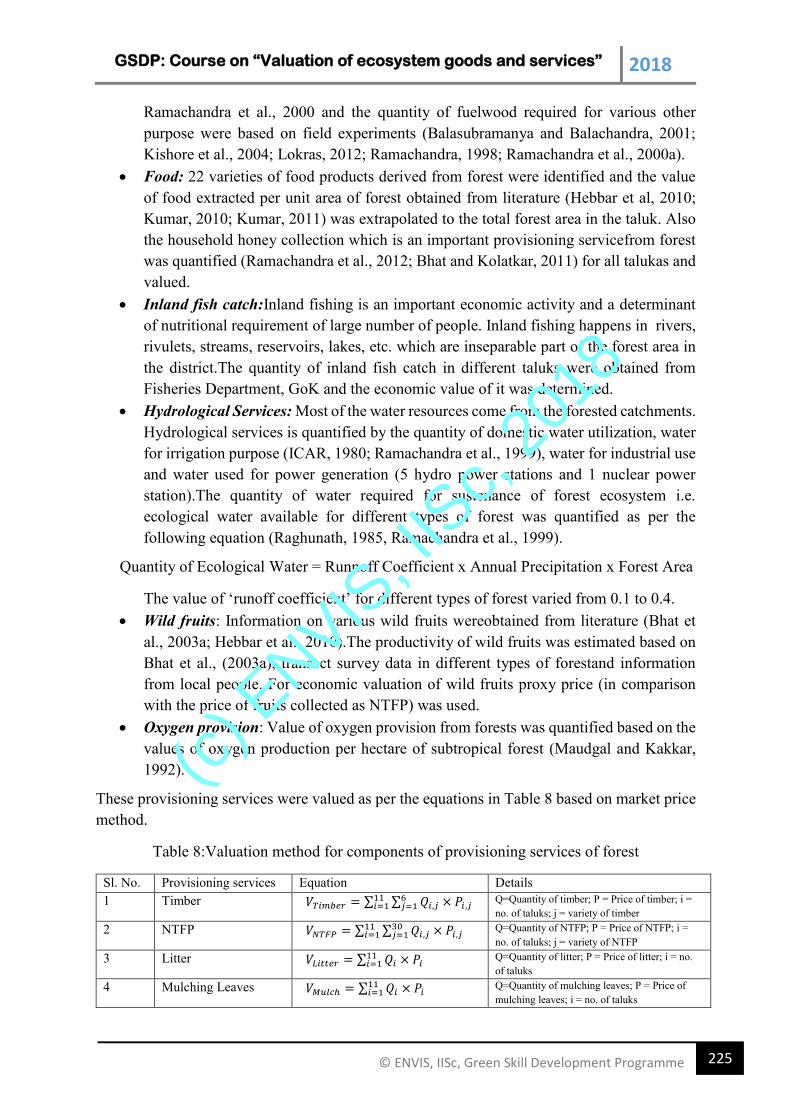
GSDP: Course on “Valuation of ecosystem goods and services” 2018
225 © ENVIS, IISc, Green Skill Development Programme
Ramachandra et al., 2000 and the quantity of fuelwood required for various other
purpose were based on field experiments (Balasubramanya and Balachandra, 2001;
Kishore et al., 2004; Lokras, 2012; Ramachandra, 1998; Ramachandra et al., 2000a).
Food: 22 varieties of food products derived from forest were identified and the value
of food extracted per unit area of forest obtained from literature (Hebbar et al, 2010;
Kumar, 2010; Kumar, 2011) was extrapolated to the total forest area in the taluk. Also
the household honey collection which is an important provisioning servicefrom forest
was quantified (Ramachandra et al., 2012; Bhat and Kolatkar, 2011) for all talukas and
valued.
Inland fish catch:Inland fishing is an important economic activity and a determinant
of nutritional requirement of large number of people. Inland fishing happens in rivers,
rivulets, streams, reservoirs, lakes, etc. which are inseparable part of the forest area in
the district.The quantity of inland fish catch in different taluks were obtained from
Fisheries Department, GoK and the economic value of it was determined.
Hydrological Services: Most of the water resources come from the forested catchments.
Hydrological services is quantified by the quantity of domestic water utilization, water
for irrigation purpose (ICAR, 1980; Ramachandra et al., 1999), water for industrial use
and water used for power generation (5 hydro power stations and 1 nuclear power
station).The quantity of water required for sustenance of forest ecosystem i.e.
ecological water available for different types of forest was quantified as per the
following equation (Raghunath, 1985, Ramachandra et al., 1999).
Quantity of Ecological Water = Runnoff Coefficient x Annual Precipitation x Forest Area
The value of ‘runoff coefficient’ for different types of forest varied from 0.1 to 0.4.
Wild fruits: Information on various wild fruits wereobtained from literature (Bhat et
al., 2003a; Hebbar et al., 2010).The productivity of wild fruits was estimated based on
Bhat et al., (2003a), transect survey data in different types of forestand information
from local people. For economic valuation of wild fruits proxy price (in comparison
with the price of fruits collected as NTFP) was used.
Oxygen provision: Value of oxygen provision from forests was quantified based on the
values of oxygen production per hectare of subtropical forest (Maudgal and Kakkar,
1992).
These provisioning services were valued as per the equations in Table 8 based on market price
method.
Table 8:Valuation method for components of provisioning services of forest
Sl. No. Provisioning services Equation Details
1 Timber 𝑉𝑇𝑖𝑚𝑏𝑒𝑟 = ∑ ∑ 𝑄𝑖,𝑗 × 𝑃𝑖,𝑗6𝑗=1
11𝑖=1 Q=Quantity of timber; P = Price of timber; i =
no. of taluks; j = variety of timber
2 NTFP 𝑉𝑁𝑇𝐹𝑃 = ∑ ∑ 𝑄𝑖,𝑗 × 𝑃𝑖,𝑗30𝑗=1
11𝑖=1 Q=Quantity of NTFP; P = Price of NTFP; i =
no. of taluks; j = variety of NTFP
3 Litter 𝑉𝐿𝑖𝑡𝑡𝑒𝑟 = ∑ 𝑄𝑖 × 𝑃𝑖11𝑖=1 Q=Quantity of litter; P = Price of litter; i = no.
of taluks
4 Mulching Leaves 𝑉𝑀𝑢𝑙𝑐ℎ = ∑ 𝑄𝑖 × 𝑃𝑖11𝑖=1 Q=Quantity of mulching leaves; P = Price of
mulching leaves; i = no. of taluks
(c) E
NVIS, I
ISc,
2018
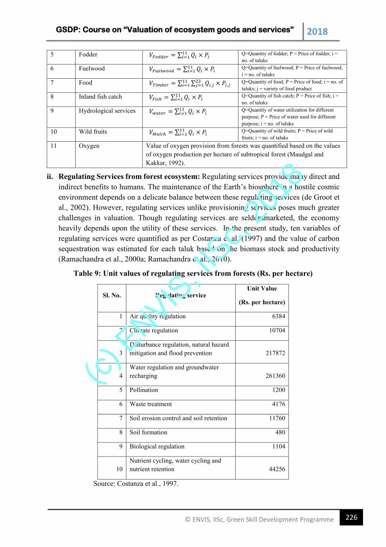
GSDP: Course on “Valuation of ecosystem goods and services” 2018
226 © ENVIS, IISc, Green Skill Development Programme
5 Fodder 𝑉𝐹𝑜𝑑𝑑𝑒𝑟 = ∑ 𝑄𝑖 × 𝑃𝑖11𝑖=1 Q=Quantity of fodder; P = Price of fodder; i =
no. of taluks
6 Fuelwood 𝑉𝐹𝑢𝑒𝑙𝑤𝑜𝑜𝑑 = ∑ 𝑄𝑖 × 𝑃𝑖11𝑖=1 Q=Quantity of fuelwood; P = Price of fuelwood;
i = no. of taluks
7 Food 𝑉𝑇𝑖𝑚𝑏𝑒𝑟 = ∑ ∑ 𝑄𝑖,𝑗 × 𝑃𝑖,𝑗22𝑗=1
11𝑖=1 Q=Quantity of food; P = Price of food; i = no. of
taluks; j = variety of food product
8 Inland fish catch 𝑉𝐹𝑖𝑠ℎ = ∑ 𝑄𝑖 × 𝑃𝑖11𝑖=1 Q=Quantity of fish catch; P = Price of fish; i =
no. of taluks
9 Hydrological services 𝑉𝑤𝑎𝑡𝑒𝑟 = ∑ 𝑄𝑖 × 𝑃𝑖11𝑖=1 Q=Quantity of water utilization for different
purpose; P = Price of water used for different
purpose; i = no. of taluks
10 Wild fruits 𝑉𝑀𝑢𝑙𝑐ℎ = ∑ 𝑄𝑖 × 𝑃𝑖11𝑖=1 Q=Quantity of wild fruits; P = Price of wild
fruits; i = no. of taluks
11 Oxygen Value of oxygen provision from forests was quantified based on the values
of oxygen production per hectare of subtropical forest (Maudgal and
Kakkar, 1992).
ii. Regulating Services from forest ecosystem: Regulating services provide many direct and
indirect benefits to humans. The maintenance of the Earth’s biosphere in a hostile cosmic
environment depends on a delicate balance between these regulating services (de Groot et
al., 2002). However, regulating services unlike provisioning services poses much greater
challenges in valuation. Though regulating services are seldommarketed, the economy
heavily depends upon the utility of these services. In the present study, ten variables of
regulating services were quantified as per Costanza et al. (1997) and the value of carbon
sequestration was estimated for each taluk based on the biomass stock and productivity
(Ramachandra et al., 2000a; Ramachandra et al., 2010).
Table 9: Unit values of regulating services from forests (Rs. per hectare)
Sl. No. Regulating service Unit Value
(Rs. per hectare)
1 Air quality regulation 6384
2 Climate regulation 10704
3
Disturbance regulation, natural hazard
mitigation and flood prevention 217872
4
Water regulation and groundwater
recharging 261360
5 Pollination 1200
6 Waste treatment 4176
7 Soil erosion control and soil retention 11760
8 Soil formation 480
9 Biological regulation 1104
10
Nutrient cycling, water cycling and
nutrient retention 44256
Source: Costanza et al., 1997.
(c) E
NVIS, I
ISc,
2018
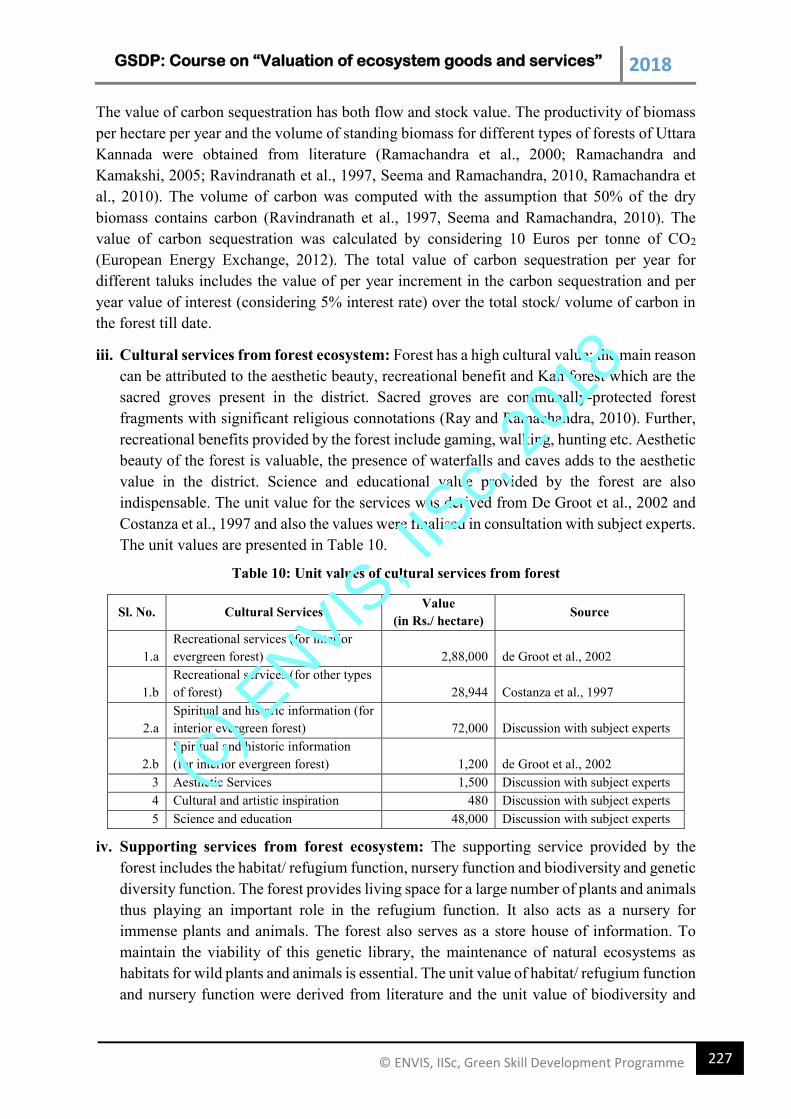
GSDP: Course on “Valuation of ecosystem goods and services” 2018
227 © ENVIS, IISc, Green Skill Development Programme
The value of carbon sequestration has both flow and stock value. The productivity of biomass
per hectare per year and the volume of standing biomass for different types of forests of Uttara
Kannada were obtained from literature (Ramachandra et al., 2000; Ramachandra and
Kamakshi, 2005; Ravindranath et al., 1997, Seema and Ramachandra, 2010, Ramachandra et
al., 2010). The volume of carbon was computed with the assumption that 50% of the dry
biomass contains carbon (Ravindranath et al., 1997, Seema and Ramachandra, 2010). The
value of carbon sequestration was calculated by considering 10 Euros per tonne of CO2
(European Energy Exchange, 2012). The total value of carbon sequestration per year for
different taluks includes the value of per year increment in the carbon sequestration and per
year value of interest (considering 5% interest rate) over the total stock/ volume of carbon in
the forest till date.
iii. Cultural services from forest ecosystem: Forest has a high cultural value; the main reason
can be attributed to the aesthetic beauty, recreational benefit and Kan forest which are the
sacred groves present in the district. Sacred groves are communally-protected forest
fragments with significant religious connotations (Ray and Ramachandra, 2010). Further,
recreational benefits provided by the forest include gaming, walking, hunting etc. Aesthetic
beauty of the forest is valuable, the presence of waterfalls and caves adds to the aesthetic
value in the district. Science and educational value provided by the forest are also
indispensable. The unit value for the services was derived from De Groot et al., 2002 and
Costanza et al., 1997 and also the values were finalised in consultation with subject experts.
The unit values are presented in Table 10.
Table 10: Unit values of cultural services from forest
Sl. No. Cultural Services Value
(in Rs./ hectare) Source
1.a
Recreational services (for interior
evergreen forest) 2,88,000 de Groot et al., 2002
1.b
Recreational services (for other types
of forest) 28,944 Costanza et al., 1997
2.a
Spiritual and historic information (for
interior evergreen forest) 72,000 Discussion with subject experts
2.b
Spiritual and historic information
(for interior evergreen forest) 1,200 de Groot et al., 2002
3 Aesthetic Services 1,500 Discussion with subject experts
4 Cultural and artistic inspiration 480 Discussion with subject experts
5 Science and education 48,000 Discussion with subject experts
iv. Supporting services from forest ecosystem: The supporting service provided by the
forest includes the habitat/ refugium function, nursery function and biodiversity and genetic
diversity function. The forest provides living space for a large number of plants and animals
thus playing an important role in the refugium function. It also acts as a nursery for
immense plants and animals. The forest also serves as a store house of information. To
maintain the viability of this genetic library, the maintenance of natural ecosystems as
habitats for wild plants and animals is essential. The unit value of habitat/ refugium function
and nursery function were derived from literature and the unit value of biodiversity and
(c) E
NVIS, I
ISc,
2018
GSDP: Course on “Valuation of ecosystem goods and services” 2018
228 © ENVIS, IISc, Green Skill Development Programme
genetic diversity was estimated based on the flow value of selected provisionservices that
represent the least value stock of biodiversity and genetic diversity. The unit values are
presented in Table 11.
Table 11: Unit value of supporting services from forest
Sl. No. Supporting Services Value
(in Rs./hectare) Source
1 Habitat/ refugium services 73104 de Groot, 2002
2 Nursery services 9360 de Groot, 2002
3 Biodiversity and genetic diversity 40000
Calculated from the flow value
selected provisioning services like
NTFP, medicinal plants, etc.
Total Economic Value
The total economic value (TEV) of forest ecosystem is obtained by aggregating provisiongoods
and services, regulating services, cultural services and supporting services.
TEV = Provisioning services + Regulating services + Cultural services + Supporting
Services
The total economic value that has been calculated for one year is divided by the area of forest
in each taluk to obtain the per hectare value of forest in respective taluk.
REFERENCES
1. Anderson, T and J Bojo. 1992. 'The Economic Value of Forests' in Anil Agarwal (edt.), The
Price of Forests, CSE, New Delhi.
2. Anitha, V. and P.K. Muraleedharan. 2006. Economic valuation of ecotourism development of
a recreational site in the natural forests of southern Western Ghats, KFRI Research Report,
Kerala Forest Research Institute, Peechi.
3. Arnold, J.E.M. and M. Ruiz Pérez. 2001. 'Can non-timber forest products match tropical forest
conservation and development objectives?', Ecological Economics, Vol. 39, No. 3, pp. 437–
447.
4. Atkinson, Giles and Haripriya Gundimeda. 2006. ‘Accounting for India's forest wealth’,
Ecological Economics, Vol. 59, No. 4, pp. 462-476.
5. Balasubramanya, M.H., and P Balachandra. 2001. An Exploratory Study of Environmental
Pollution by Small Scale Industries Sector in Karnataka, EERC Working Paper Series: IPP-2,
IGIDR, Mumbai.
6. Bauhus, J., Peter Van der Meer and M. Kanninen. 2010. Ecosystem goods and services from
plantation forest. Earthscan, London.
7. Beerappa, M. and A.G. Koppad. 2009. 'Assessment of fuel wood collection on depletion of
forest resources in Uttara Kannada district', Karnataka Journal of Agricultural Sciences. Vol.
22, No. 4, pp. 935-936.
8. Bhat, P. R. and Milind Kolatkar. 2011. Performance and problems of the bee keeping industry
in Karnataka, CES Technical Report No. 124, CES, IISc, Bangalore.
9. Bhat, D.M., N.S. Prasad, M. Hegde, C.J. Saldanha. 1984. Plant diversity studies in Uttara
Kannada district, CES Technical Report No. 9, CES, IISc, Bangalore.
(c) E
NVIS, I
ISc,
2018
GSDP: Course on “Valuation of ecosystem goods and services” 2018
229 © ENVIS, IISc, Green Skill Development Programme
10. Bhat, D. M., K. S. Murali and N. H. Ravindranath. 2003. 'Carbon stock dynamics in tropical
rain forest of Uttara Kannada district, Western Ghats, India', International Journal of
Environment and Pollution,Vol. 19, No. 2, pp. 139-149.
11. Bhat, P. R., K. S. Murali, G. T. Hegde, C. M. Shastri, D. M. Bhat, Indu K. Murthy and N. H.
Ravindranath. 2003a. 'Annual variation in non-timber forest product yield in Western Ghats,
Karnataka, India', Current science,Vol. 85, No. 9, pp. 1350-1355.
12. Bourgeon, G. 1989. Explanatory booklet on the reconnaissance soil map of forest area:
Western Karnataka and Goa,French Institute, Pondicherry.
13. Boominathan M., M.D. Subash Chandran and T.V. Ramachandra. 2008. Economic valuation
of bivalves in the Aghnashini Estuary, West Coast, Karnataka, ENVIS Technical Report No.
30, Environmental Information System, CES, Bangalore.
14. CBD (Secretariat of the Convention on Biological Diversity). 2001. The Value of Forest
Ecosystems. CBD Technical series number-4, Secretariat of the Convention
on Biological Diversity, Montreal.
15. Champion, H. and S.K. Seth. 1968. A revised survey of the forest types of India. Govt. of India
Publication, New Delhi.
16. Chandran, M. D. S. 1984. Ecosystem studies and management in Coastal Uttara Kannada. CES
Technical Report No. 3, CES, IISc, Bangalore.
17. Chandran, M. D. S. 1987. The Impact of Forest based industries on the Evergreen Forest of
Uttara Kannada. CES Technical Report No. 34, CES, IISc, Bangalore.
18. Chandran, M. D. S. 1993. Vegetational changes in the evergreen forest belt of the Uttara
Kannada District of Karnataka State, Ph.D. Thesis submitted to Karnataka University,
Dharwad, India.
19. Chandran M.D.S., G.R. Rao, K.V. Gururaja and T.V. Ramachandra. 2010. ‘Ecology of the
Swampy Relic Forests of Kathalekan from Central Western Ghats, India', Bioremediation,
Biodiversity and Bioavailability, Vol. 4, No. 1 (Special Issue), Global Science Books, pp. 54-
68.
20. Costanza, R., R d’Arge, R de Groot, S Farberk, M Grasso, B Hannon, K Limburg, S Naeem, R
V. O’Neill, J Paruelo, R G. Raskin, P Suttonkk and M van den. Belt. 1997. 'The value of the
world’s ecosystem services and natural capital', Nature, Vol. 387, No. 6630, pp. 253-260.
21. Daily, G.C., P.A. Matson. 2008. Ecosystem services: from theory to implementation. PNAS,
Vol. 105, No. 28, pp. 9455–9456.
22. Daniels, R.J.R. 1989. A Conservation Strategy for the Birds of Uttara Kannada district, Ph.D.
Thesis, Centre for Ecological Science, Indian Institute of Science, Bangalore.
23. Daniels, R.J.R., Malati Hegde, N.V. Joshi and Madhav Gadgil. 1991. 'Assigning conservation
value: A case study from India', Conservation Biology, Vol. 5, No. 4, pp. 464-475.
24. de Groot, R. S., Matthew A. Wilson, Roelof M.J. Boumans. 2002. 'A typology for the
classification, description and valuation of ecosystem functions, goods and services',
Ecological Economics, Vol. 41, No. 3, pp. 393–408.
25. DEFRA. 2007. An Introductory Guide to Valuing Ecosystem Services, Department for
Environment, Food and Rural Affairs, London.
26. Djafar, Febi. 2006. Cultural Services of Forests: A case study in Garhwal Hills, Uttaranchal,
India. NETFOP Report 07. Alterra, Wageningen UR
27. FAO. 1990. The major significance of Minor Forest roduct. The local use and value of forest
in the West African Humid Forest Zone, Community Forestry Note 6, FAO, Rome.
28. FAO. 2000. On definitions of forest and forest change. FRA Working Paper 33. FAO, Rome.
29. FAO. 2010. Global Forest Resources Assessment-2010, Forestry Paper 163, FAO, Rome.
(c) E
NVIS, I
ISc,
2018
GSDP: Course on “Valuation of ecosystem goods and services” 2018
230 © ENVIS, IISc, Green Skill Development Programme
30. Fontaine, B., P Bouchet, K V Achterberg, M A Alonso-Zarazaga, R Araujo, M Asche, U
Aspock, P Audisio and others. 2007. 'The European union’s 2010 target: putting rare species in
focus', Biological Conservation, Vol. 139, No. 1-2, pp. 167–185.
31. Fischlin, A., G.F. Midgley, J.T. Price, R. Leemans, B. Gopal, C. Turley, M.D.A. Rounsevell,
O.P. Dube, J. Tarazona, A.A. Velichko. 2007. Ecosystems, their properties, goods, and services
in M.L. Parry, O.F. Canziani, J.P. Palutikof, P.J. van der Linden and C.E. Hanson (Eds.),
Climate Change 2007: Impacts, Adaptation and Vulnerability. Contribution of Working Group
II to the Fourth Assessment Report of the Intergovernmental Panel on Climate Change,
Cambridge University Press, Cambridge.
32. Gera, Mohit., Akhilesh Yadav, N. S. Bisht and Giresh Mohan. 2008. 'Valuation of recreational
benefits from the Valley of flowers National Park', The Indian forester, Vol: 134, No. 1, pp.
26-35.
33. Gonzalez, Patrick., R Hassan, P Lakyda, I McCallum, S Nilsson, J Pulhin, B Rosenburg and B
Scholes. 2005. Forest and Woodland Systems in Hassan, R., R. Scholes and N. Ash, Eds.
Ecosystems and Human Wellbeing: Volume 1: Current State and Trends. Island Press,
Washington.
34. Haripriya, G.S. 2001. 'Integrated Environmental and Economic Accounting: An Application to
the Forest Resources in India', Environmental and Resource Economics, Vol. 19, No. 1, pp. 73-
95.
35. Haripriya, G. S. 2002. ‘Biomass carbon of truncated diameter classes in Indian forests’, Forest
Ecology and Management, Vol. 168, No. 1-3, pp. 1-13.
36. Harsha, V.H., S.S. Hebbar, G.R. Hegde, V Shripathy. 2002. 'Ethno medical knowledge of plants
used by Kunabi tribe of Karnataka in India', Fitoterapia, Vol. 73, No. 4, pp. 281-287.
37. Harsha, V.H., S.S. Hebbar, V. Shripathi and G.R. Hegde. 2003. 'Ethnomedicobotany of Uttara
Kannada district in Karnataka, India', Journal of Ethnopharmacology, Vol. 84, No. 1, pp. 37-
40.
38. Harsha, V.H., V. Shripathy and G.R. Hegde. 2005. 'Ethno veterinary practices in Uttara
Kannada district of Karnataka', Indian Journal of Traditional Knowledge, Vol. 4, No. 3, pp.
253-258.
39. Hassan, R., R. Scholes and N. Ash (Eds.). 2005. Ecosystems and Human Wellbeing: Volume
1: Current State and Trends. Island Press, Washington.
40. Hebbar, S.S., G. Hegde and G.R.Hegde. 2010. 'Less known wild edible fruits and seeds of
Uttara Kannada district', Indian Forester, Vol. 136, No. 9, pp. 1218-1222.
41. Hegde, H.V., G.R. Hegde and S.D. Kholkute. 2007. 'Herbal care for reproductive health:
Ethnomedicobotany from Uttara Kannada', Complementary Therapies in Clinical Practice,
Vol. 13, No. 1, pp. 38-45.
42. ICAR. 1980. Handbook of Agriculture, Indian Council of Agricultural Research, New Delhi.
43. International Energy Agency (IEA). 1998. Energy statistics and balances of non-OECD
Countries 1995-1996. IEA, Paris.
44. Inamati, S. S., K. V. Devar, A. Krishna. 2005. 'Regeneration frequency and stand composition
of tree species in Devimane Ghat of Uttara Kannada', Karnataka Journal of Agricultural
Sciences,Vol. 18, No. 4, pp, 1155-1159.
45. Jana, Bipal Kr., Soumyajit Biswas, Mrinmoy Majumder, Pankaj Kr Roy and Asis Mazumdar.
2009. 'Carbon sequestration rate and above ground biomass carbon potential of four young
species', Ecological Economics, Vol. 1, No. 22, pp. 112-118.
46. Kamath, S. U. (edt.). 1985. Uttara Kannada District. Karnataka State Gazetteer. Government
of Karnataka, Bangalore.
(c) E
NVIS, I
ISc,
2018
GSDP: Course on “Valuation of ecosystem goods and services” 2018
231 © ENVIS, IISc, Green Skill Development Programme
47. Kant,S., J Nautiyal, and R.Berry. 1996. 'Forests and economic welfare', Journal of Economic
Studies, Vol. 23, No. 2, pp. 31-43.
48. Kishore, V.V.N., Preety M. Bhandari and Pratul Gupta. 2004.'Biomass energy technologies for
rural infrastructure and village power—opportunities and challenges in the context of global
climate change concerns', Energy Policy, Vol. 32, No. 6, pp. 801-810.
49. Kramer, R., Munasinghe, M., Sharma, N., Mercer, E. and Shyamsundar, P. (1992), 'Valuing a
Protected Tropical Forest: A Case Study in Madagascar', paper presented at the IVth World
Congress on National Parks and Protected Areas, 10-21 February, Caracas, Venezuela.
50. Kramer, R., Sharma, N. and Munasinghe, M. (eds.) (1995), “Valuing Tropical Forests:
Methodology and Case Study of Madagascar,” Environment Paper No. 13. World Bank,
Washington D.C.
51. Kruijssen F and Mysore S. 2010. Integrating biodiversity conservation and livelihood
improvement: The role of markets for mango varieties and Garcinia species in India.
Biodiversity International, India.
52. Kumar, Bharath L.B. 2010. Impact of non-timber forest products on tribal economy: An
econometric analysis in western-ghats of Karnataka, M.Sc. Thesis submitted to University of
Agricultural Sciences, Dharwad.
53. Kumar, Bharath L. B., B. L. Patil, H. Basavaraja, S. M. Mundinamani, S. B. Mahajanashetty
and S. N. Megeri. 2011. 'Participation behaviour of indigenous people in non-timber forest
products extraction in western ghats forests', Karnataka Journal of Agricultural Sciences, Vol.
24, No. 2, pp. 170-172.
54. Kumar, P. 2004. 'Valuation of medicinal plants for pharmaceutical uses', Current Science, Vol.
86, No. 7, pp. 930-937.
55. Kumar, Pushpam., Madhu Verma, M D Wood and D Negandhi. 2010. Guidance Manual for
the Valuation of Regulating Services. UNEP, Nairobi.
56. Kumar, Manasi. and Pushpam Kumar. 2008. ‘Valuation of the ecosystem services: A psycho-
cultural perspective’, Ecological Economics, Vol. 64, No. 4, pp. 808-819.
57. Lakshamana, A. C. 2007. Challenges of Rattan Conservation and Development: Guidelines and
Policies,
Source:https://www1.inbar.int/news/proceedings_guangzhou/3CHALLENGES_OF_RATTA
N_CONSERVATION_AND_DEVELOPMENT.ppt, accessed on 02.10.2012
58. Lal, J. B. 1992. Economic value of India’s forest stock in Anil Agarwal (edt.), The Price of
Forests by CSE, New Delhi.
59. Lal, M. and Roma Singh. 2000. 'Carbon sequestration potential of Indian forests',
Environmental Monitoring and Assessment, Vol. 60, No. 3, pp. 315-327.
60. Lele, S. M. 1993. Degradation, Sustainability or transformation? A case study of villager’s use
of Forest lands in Malnad Region of Uttara Kannada district, India, CES Technical Report
No.27, CES, IISc, Bangalore
61. Lokras, S.S. 2012. 'Development and Dissemination of Fuel-Effcient Biomass Burning
Devices', Journal of Indian Institute of Science, Vol. 92, No. 1, pp. 99-110.
62. Mace, G.M., 2005. 'Biodiversity: An index of intactness', Nature, Vol. 434, No. 7029, pp. 32–
33.
63. Mahapatra, A. K. and D. D. Tewari. 2005. 'Importance of non-timber forest products in the
economic valuation of dry deciduous forest of India', Forest policy and Economics, Vol. 7, No.
3, pp. 455-467.
(c) E
NVIS, I
ISc,
2018
GSDP: Course on “Valuation of ecosystem goods and services” 2018
232 © ENVIS, IISc, Green Skill Development Programme
64. Manjunatha, G. O., V. M. Dabgar, V. M. Dasar and S. K. Patil. 2009. 'Conservation of NWFP
species through sustainable harvesting and cultivation in farm and betta lands in Uttara
Kannada district', My Forest, Vol.45, No. 4, pp. 437-444.
65. Manjunatha, G. O., V. Suryanarayana, G. V. Dasar, S. K. Patil and Nagaraja Hegde. 2009.
'Important indigenous tree species of medicinal importance and their utilization in Uttara
Kannada district', My Forest, Vol. 45, No. 4, pp. 475-484.
66. Manoharan, T.R. 1996. 'Economics of Protected Areas: A case Study of Periyar Tiger Reserve',
Ph. D. Thesis. Forest Research Institute, Dehra Dun.
67. Marigoudra, R., Sanjeev Kyatappanavar, R Rathod and A Krishna. 2004. 'Vegetation studies in
Bairumbe in Uttara Kannada', Karnataka Journal of Agricultural Sciences, Vol. 17, No. 4, pp.
878-880.
68. Mas, Margarita Triguero., Marc Olomi Sola and V.R. Garcia. 2007. Local Perception in
Dandeli Wildlife Sanctuary, Karnataka, India. Universitat Autònoma de Barcelona.
69. Mas, Margarita Triguero., Marc Olomi Sola, Naveen Jha, Francisco Zorondo Rodriguez And
V Ictoria Reyes Garcia. 2009. 'Urban and rural perceptions of protected areas: A case study in
Dandeli Wildlife Sanctuary, India', Environmental conservation, Vol. 36, No. 3 pp. 208-217.
70. Maudgal, S and Meenakshi Kakkar. 1992. Evaluation of forests for impact assessment of
development project in Anil Agarwal (edt.), The Price of Forests, CSE, New Delhi.
71. MEA (Millennium Ecosystem Assessment). 2003. Ecosystems and Human Well-Being: A
Framework for Assessment, Island Press, Washington, DC
72. Mohandas, T. V. and O. K. Remadevi. 2011. 'A study on tourist visitations in protected areas
of central western ghats in Karnataka', The Indian Forester, Vol. 137, No. 4, pp. 403-410.
73. Murali, K.S., D.M. Bhat and N.H. Ravindranath. 2000. 'Biomass estimation equations for
tropical deciduous and evergreen forest'. International Journal of Agricultural Resources,
Governance and Ecology. Vol. 4, No. 1, pp. 81-90.
74. Murthy, I.K., P.R. Bhat, N.H. Ravindranath and R. Sukumar. 2005. 'Financial valuation of non-
timber forest product flows in Uttara Kannada district, Western Ghats, Karnataka', Current
Science, Vol. 88, No. 10, pp. 1573-1579.
75. Myers, N. 1984. The primary source: Tropical forests and our future, W.W.Norton, New York.
76. Nadkarni, M. V. and S. A. Pasha. 1992. Contribution of forest to Agriculture: A study of
Arecanut gardens in Uttara Kannada in Anil Agarwal (edt.), The Price of Forests,CSE, New
Delhi.
77. Nasi, R., S Wunder and J. J. Campos. 2002. Forest ecosystem services: Can they pay our way
out of deforestation? A discussion paper prepared for the Forestry Roundtable held in
conjunction with the UNFF II, Costa Rica on March 11, 2002.
78. Newcome, Jodi., Allan Provins, Helen Johns, Ece Ozdemiroglu, Jaboury Ghazoul, Diane
Burgess and Kerry Turner. 2005. The Economic, Social and Ecological Value of Ecosystem
Services: A Literature Review, Economics for the Environment Consultancy, London.
79. Prasad, S. N., M. S. Hedge, Madhav Gadgil and K. M. Hegde. An Experiment in
Ecodevelopment in Uttara Kannada district of Karnataka, CES Technical Report No. 2, CES,
IISC, Bangalore.
80. Prasad, S. N., M Hedge and M.S. Hedge. 1987. Fuel consumption and Conservation method in
urban centres of Uttara Kannada, CES Technical Report 25. CES, IISc, Bangalore.
81. Nayak, R.B. 2008. Characterization of soils, cultivation practices and productivity of rice
(Oryza sativa) in Upghat region of Uttara Kannada district. M.Sc. Thesis submitted to
University of Agricultural Sciences, Dharwad.
(c) E
NVIS, I
ISc,
2018
GSDP: Course on “Valuation of ecosystem goods and services” 2018
233 © ENVIS, IISc, Green Skill Development Programme
82. Panchamukhi, P, R., P Trivedi, S Debi, A.K. Kulkarni, and P Sharma. 2008. Natural resource
accounting in Karnataka: A study on land and forestry sector (Excluding mining), Centre for
Multi-Disciplinary Development Research, Dharwad.
83. Pascal, J.P. 1984. Explanatory Booklet on the Forest Map of South India: Belgaum-Dharwar-
Panaji, Shimoga, Mercara-Mysore. Karnataka Forest Department and the French Institute,
Pondicherry.
84. Pearce, D.W., D Moran and Dan Biller. 2002. Handbook of biodiversity valuation: A guide for
policy makers, OECD, Paris.
85. Pearce, David and Dominic Moran. 1994. The Economic Value of Biodiversity. IUCN-The
World Conservation Union. Earthscan, London.
86. Pearce, D.W. and Pearce, C. (eds.) 2001. Valuing environmental benefits: case studies from the
developing world. Edward Elgar, Cheltenham.
87. Peters, C.M., A. H. Gentry and R. O. Mendelsohn. 1989. ‘Valuation of an Amazonian
rainforest’, Nature, Vol. 339, No.6227, pp. 655-656.
88. Pittini, Michele. 2011. Monetary Valuation for Ecosystem Accounting. Issue paper prepared
for the UN/World Bank/EEA Expert Meeting on Ecosystem Accounts, London, December
2011.
89. Pomeroy, M., R Primack, and S.N. Rai. 2003. 'Changes in four rainforest plots of the Western
Ghats, India, 1939-1993', Conservation and Society, Vol. 1, No. 1, pp. 113-135.
90. Prasad, N. S., H.G. Hegde, D.M. Bhat, and M Hegde. 1987. Estimates of standing biomass and
productivity of tropical moist forest of Uttara Kannada district, Karnataka, India, CES
Technical Report No. 19, CES, IISc, Bangalore.
91. Raghunath, H.M. 1985. Hydrology, Wiley Eastern Limited, New Delhi.
92. Raghu, C. 2006. Economics of production and marketing of Patchouli in North Karnataka.
M.Sc. Thesis submitted to University of Agricultural Sciences, Dharwad.
93. Rai, N.D. and C.F. Uhl. 2004. Forest product use, conservation and livelihood: The case of
uppage fruit harvest in the Western Ghats, India, Conservation and society, Vol. 2, No. 2, pp.
289-313.
94. Rajesh, D, B. 2006. Economic evaluation of vanilla cultivation in Uttara Kannada district of
Karnataka. M.Sc. Thesis submitted to University of Agricultural Sciences, Dharwad.
95. Ramachandra T.V. 2007. Vegetation Status in Uttara Kannada District, Mapana Journal of
Sciences, Vol. 6, No. 1, pp. 1-26.
96. Ramachandra, T.V. 1998. 'Energy utilisation in rural industries in Karnataka', International
Journal of Ambient Energy, Vol. 19, No. 2, pp.75-92.
97. Ramachandra, T. V. and Savitha Ganapathy. 2007. Vegetation analysis in Uttara Kannada
district using GIS and remote sensing techniques, ENVIS Technical Report No. 24,
Environmental Information System, CES, IISc, Bangalore.
98. Ramachandra, T.V. and A.V. Nagarathna. 2001. 'Energetics in paddy cultivation in Uttara
Kannada District', Energy Conversion and Management, Vol. 42, No. 2, pp. 132-155.
99. Ramachandra, T.V., D.K. Subramanian, N.V. Joshi, S.V. Gunaga and R.B. Harikanta. 2000.
'Domestic energy consumption patterns in Uttara Kannada district, Karnataka state, India',
Energy Conservation and Management, Vol. 41, No. 8, pp. 775-831.
100. Ramachandra, T.V., N.V. Joshi, D.K. Subramanian. 2000a. 'Present and prospective role of
bioenergy in regional energy system', Renewable and Sustainable Energy Reviews, Vol. 4, No.
4, pp. 375-430.
(c) E
NVIS, I
ISc,
2018
GSDP: Course on “Valuation of ecosystem goods and services” 2018
234 © ENVIS, IISc, Green Skill Development Programme
101. Ramachandra, T.V., G. Kamakshi and B.V. Shruthi. (2004). 'Bioresource status in Karnataka',
Renewable and Sustainable Energy Reviews, Vol. 8, No. 1, pp. 1-47.
102. Ramachandra, T, V., R. Rajinikanth and V. G. Ranjini. 2005. 'Economic Valuation of
Wetlands', Journal of Environmental Biology, Vol. 26, No. 2, pp. 439-447.
103. Ramachandra T.V., M. D. Subash Chandran, K V Gururaja and Sreekantha. 2007. Cumulative
Environmental Impact Assessment, Nova Science Publishers, New York.
104. Ramachandra, T, V., B. Alakananda, Ali Rani, M. A. Khan. 2011. 'Ecological and Socio-
Economic Assessment of Varthur Wetland, Bengaluru , India', Journal of Environmental
Science and Engineering,Vol. 53, No. 1, pp. 101-108.
105. Ramachandra, T. V., M.D. Subhash Chandran, N.V. Joshi and Balachandran. C. 2012.
Beekeeping: Sustainable Livelihood Option in Uttara Kannada, Central Western Ghats. ENVIS
Technical Report No. 19, Environmental Information System, CES, IISc, Bangalore.
106. Ramana, P. and S. K. Patil. 2008. 'Marketing of value added products from Artocarpus species
in Uttara Kannada district of Karnataka', My Forest, Vol. 44, No.1, pp. 49-53.
107. Rao., G.R., Divaker Mesta, M.D.Subhash Chandran and T. V. Ramachandra. 2008. Wetland
flora of Uttara Kannada in T. V. Ramachandra (ed.), Environmental Education for Ecosystem
Conservation. Capital Publishing Company, New Delhi.
108. Rao, D.N. 1990. 'Economics of forest products in India: Issues and Perspectives', in Anil
Agarwal (edt.), The Price of Forests,CSE, New Delhi, pp. 75-84.
109. Ravindranath, N.H., B.S. Somashekhar and Madhav Gadgil. 1997. 'Carbon flow in Indian
forests',Climatic Change, Vol. 35, No. 3, pp. 297-320.
110. Ray, Rajasri. and T. V. Ramachandra. 2011. ‘Small sacred goves in local landscape: are they
really worth for conservation?’, Current Science, Vol. 98, No. 9, pp. 1178-1180.
111. Ray, Rajasri., M.D.Subhash Chandran and T. V. Ramachandra. 2011. Sacred goves in Siddapur
Taluk, Uttara Kannada, Karnataka: Threats and Management Aspects, ENVIS Technical
Report 38, Environmental Information System, CES, IISc, Bangalore.
112. Riera, P. 2001. Assessment of methodologies for valuing biological diversity of forest: Report
to work programme on conservation and enhancement of biology and landscape diversity in
forest ecosystems, Internal Report No. 2, European Forest Institute, Finland.
113. Seema, D. and T.V. Ramachandra. 2010. Carbon sequestration potential of ecosystems in
Uttara Kannada district, Western Ghats of Karnataka, India. Conference paper, Lake 2010,
Bangalore.
114. Shackleton, S., C. Shackleton and B. Cousins. 2000. ‘Revaluing the communal lands of
southern Africa: new understandings of rural livelihoods’, ODI Natural Resource Perspectives
No. 62. The Overseas Development Institute, London.
115. Shastri, C.M., D.M. Bhat, B.C. Nagaraja, Murali, K,S; Ravindranath, N, H. 2002. 'Tree species
diversity in a village ecosystem in Uttara Kannada district in Western Ghats, Karnataka',
Current Science, Vol. 82, No. 9, pp. 1080-1083.
116. Simpson, R.D., Roger A. Sedjo and John W. Reid. 1996. 'Valuing biodiversity for use in
Pharmaceutical Research', The Journal of Political Economy, Vol. 104, No. 1, pp. 163-185.
117. Swamy, S. L., C.B.S. Dutt, M.S.R. Murthy, A. Mishra, S.S. Bargali. 2010. 'Floristic and dry
matter dynamics of tropical wet evergreen forest of Western Ghats, India', Current Science,
Vol. 99, No. 3, pp. 353-354.
118. TEEB. 2010. The Economics of Ecosystems and Biodiversity: Ecological and Economic
Foundations, London and Washington: Earthscan.
(c) E
NVIS, I
ISc,
2018
GSDP: Course on “Valuation of ecosystem goods and services” 2018
235 © ENVIS, IISc, Green Skill Development Programme
119. Tewari, D.O. and J.Y Campbell. 1996. 'Increased development of non-timber forest products
in India: Some issues and concern', Unasylva, Vol. 47, No. 187, pp. 26-31.
Source:http://www.fao.org/docrep/w2149e/w2149e06.htm#increased development of non timber forest
products in india: some issues and co accessed on 17.11.2012
120. UNDP (United Nations Development Programme). 2000. World energy assessment: energy
and the challenge of sustainability, UNDP, Department of Economic and Social and Affairs
and World Energy Council, New York.
121. UNEP. 2008. IEA Training Manual: A training manual on integrated environmental assessment
and reporting, UNEP-IISD.
122. USFWS. 1995. A manual for conducting Natural Resource Damage Assessment: The role of
Economics. Fish and Wildlife Service, US Department of Interior.
123. Varadaranganatha, G.H. and S.L. Madiwalar. 2010. 'Studies on species richness, density and
density of tree/ shrub species in agro forestry systems'. Karnataka Journal of Agricultural
Sciences, Vol. 23, No. 3, pp. 452-456.
124. Ved, D.K., A. Mudappa and A. Singh. 2002. Trade status of commercially important medicinal
plant species of the project area of Andhra Pradesh community forest management project,
FRLHT, Bangalore.
125. Verma, Madhu., Shailendra Joshi, Girija Godbole and Aman Singh. 2007. Valuation of
Ecosystem Services and Forest Governance: A scoping study from Uttarakhand, LEAD India,
2007.
126. WEHAB. 2002. 'A Framework for Action on Biodiversity and Ecosystem Management',
Water, Energy, Health, Agriculture and Biodiversity Working Group Report, contribution to
the World Summit on Sustainable Development, Johannesburg, South Africa, 26 August – 4
September 2002. United Nations, New York.
(c) E
NVIS, I
ISc,
2018
Appraisal of Forest Ecosystems Goods and Services:Challenges and Opportunities for Conservation
T. V. Ramachandra1,2,3, Divya Soman, Ashwath D. Naik1 and M. D. Subash Chandran1
1Energy & Wetlands Research Group, Centre for Ecological Sciences (CES)2Centre for Sustainable Technologies (ASTRA)
3Centre for infrastructure, Sustainable Transportation and Urban Planning (CiSTUP)Indian Institute of Science, Bangalore 560 012, Karnataka, India
Telephone: 91-80-23600985, 22932506, 22933099, Fax: 91-80-23601428, 23600085,23600683[CES-TVR], E-mail: <[email protected]>,<[email protected]>
KEYWORDS Economic Valuation. Provisioning Services. Regulating Services. Tropical Forests
ABSTRACT Valuation of ecosystem goods and services is essential to formulate sustainable development policiesoriented towards the protection or restoration of ecosystems. The present study estimates the value of forestecosystem of Uttara Kannada district by market price method. The total value of provisioning goods and servicesfrom the forests of Uttara Kannada district was estimated at Rs. 15,171 crores per year, which amounts to aboutRs. 2 lakh per hectare per year. The study highlights the undervaluation of forest goods and services that is evidentwhen the estimated total economic value of forest and the value of forest resources calculated in national incomeaccounting framework are compared. The quantification of all benefits associated with the forest ecosystem goodsand services would help in arriving at an appropriate policy and managerial decisions to ensure conservation whileopting sustainable development path.
INTRODUCTION
An ecosystem is a complex of interconnect-ed living organisms inhabiting a particular areaor unit space, together with their environmentand all their interrelationships and relationshipswith the environment having well-maintainedecological processes and interactions (Ram-achandra et al. 2007, 2015). Ecosystem functionsinclude the exchange of energy between theplants and animals that are needed for the suste-nance of life. These functions include nutrientcycling, oxygen regulation, water supply etc. Theflow of goods or services which occur naturallyby ecological interactions between biotic andabiotic components in an ecosystem is often re-ferred as ecosystem goods and services. Thesegoods and services not only provide tangibleand intangible benefits to human community, butalso are critical to the functioning of ecosystem.Thus, ecosystem goods and services are theprocess through which natural ecosystems andthe species that make up sustain and fulfill thehuman needs (Newcome et al. 2005). Ecosystemsare thus natural capital assets supporting andsupplying services highly valuable to humanlivelihoods and providing various goods and
services (MEA 2003; Daily and Matson 2008;Gunderson et al. 2016). The tropical forests arethe rich source of biodiversity and are probablythought of containing more than half of world’sbiodiversity. Biodiversity is important to humankind in fulfilling its needs by way of providingfood (80,000 species), medicine (20,000 species),drug formulations (8,000 species) and raw mate-rials (90% from forests) for industries (Ram-achandra et al. 2016a, b; Ramachandra and Na-garathna 2001: Ramachandra and Ganapathy2007). Among the terrestrial biomes, forests oc-cupy about 31 percent (4,033 million hectare) ofthe world’s total land area and of which 93 per-cent of the world’s forest cover is natural forestand 7 percent is planted (FAO 2010; TEEB 2010;Villegas-Palacio et al. 2016). Forest ecosystemsaccount for over two-thirds of net primary pro-duction on land – the conversion of solar ener-gy into biomass through photosynthesis, mak-ing them a key component of the global carboncycle and climate (MEA 2003). The forests ofthe world harbor very large and complex biolog-ical species diversity, which is an indicator forbiological diversity and the species richnessincreases as we move from the poles to the equa-torial region. Forest ecosystem services can pro-
J Biodiversity, 8(1): 12-33 (2017) 10.1080/09766901.2017.1346160DOI:
Dow
nloa
ded
by [
Indi
an I
nstit
ute
of S
cien
ce],
[T
. V. R
amac
hand
ra]
at 0
7:01
26
Sept
embe
r 20
17
236
(c) E
NVIS, I
ISc,
2018
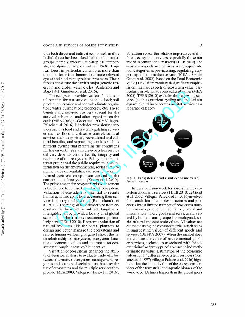
GOODS AND SERVICES OF FOREST ECOSYSTEMS 13
vide both direct and indirect economic benefits.India’s forest has been classified into four majorgroups, namely, tropical, sub-tropical, temper-ate, and alpine (Champion and Seth 1968). Trop-ical forest in particular contributes more thanthe other terrestrial biomes to climate relevantcycles and biodiversity related processes. Theseforests constitute the earth’s major genetic res-ervoir and global water cycles (Anderson andBojo 1992; Gunderson et al. 2016).
The ecosystem provides various fundamen-tal benefits for our survival such as food; soilproduction, erosion and control; climate regula-tion; water purification; bioenergy, etc. Thesebenefits and services are very crucial for thesurvival of humans and other organisms on theearth (MEA 2003; de Groot et al. 2002; Villegas-Palacio et al. 2016). It includes provisioning ser-vices such as food and water, regulating servic-es such as flood and disease control, culturalservices such as spiritual, recreational and cul-tural benefits, and supporting services such asnutrient cycling that maintains the conditionsfor life on earth. Sustainable ecosystem servicedelivery depends on the health, integrity andresilience of the ecosystem. Policy-makers, in-terest groups and the public require reliable in-formation on the environmental, social and eco-nomic value of regulating services to make in-formed decisions on optimum use and on theconservation of ecosystems (Kumar et al. 2010).The prime reason for ecosystem mismanagementis the failure to realise the value of ecosystem.Valuation of ecosystem is essential to respitehuman activities apart from accounting their ser-vices in the regional planning (Ramachandra etal. 2011). The range of benefits derived from ec-osystem can be direct or indirect, tangible orintangible, can be provided locally or at globalscale – all of which makes measurement particu-larly hard (TEEB 2010). Economic valuation ofnatural resources aids the social planners todesign and better manage the ecosystems andrelated human wellbeing. Figure 1 shows the in-terrelationship of ecosystem, ecosystem func-tions, economic values and its impact on eco-system through incentive/disincentive.
Valuation of ecosystems enhances the abili-ty of decision-makers to evaluate trade-offs be-tween alternative ecosystem management re-gimes and courses of social action that alter theuse of ecosystems and the multiple services theyprovide (MEA 2003; Villegas-Palacio et al. 2016).
Valuation reveal the relative importance of dif-ferent ecosystem services, especially those nottraded in conventional markets (TEEB 2010).Theecosystem goods and services are grouped intofour categories as provisioning, regulating, sup-porting and information services (MEA 2003; deGroot et al. 2002), based on the Total EconomicValue (TEV) framework with significant empha-sis on intrinsic aspects of ecosystem value, par-ticularly in relation to socio-cultural values (MEA2003). TEEB (2010) excludes the supporting ser-vices (such as nutrient cycling and food-chaindynamic) and incorporates habitat service as aseparate category.
Integrated framework for assessing the eco-system goods and services (TEEB 2010; de Grootet al. 2002; Villegas-Palacio et al. 2016) involvesthe translation of complex structures and pro-cesses into a limited number of ecosystem func-tions namely production, regulation, habitat andinformation. These goods and services are val-ued by humans and grouped as ecological, so-cio-cultural and economic values. All values areestimated using the common metric, which helpsin aggregating values of different goods andservices (DEFRA 2007). When the market doesnot capture the value of environmental goodsor services, techniques associated with ‘shad-ow pricing’ or ‘proxy price’ are used to indirectlyestimate its value. Estimation of the economicvalues for 17 different ecosystem services (Cos-tanza et al.1997; Villegas-Palacio et al. 2016) high-light that the annual value of the ecosystem ser-vices of the terrestrial and aquatic biomes of theworld to be 1.8 times higher than the global gross
Fig. 1. Ecosystems health and economic valuesSource: Author
Dow
nloa
ded
by [
Indi
an I
nstit
ute
of S
cien
ce],
[T
. V. R
amac
hand
ra]
at 0
7:01
26
Sept
embe
r 20
17
237
(c) E
NVIS, I
ISc,
2018
14 T. V. RAMACHANDRA, DIVYA SOMAN, ASHWATH D. NAIK ET AL.
national product (GNP). About 63 percent of theestimated values of ecosystem services werefound to be contributed by the marine ecosys-tems while, about 38 percent of the estimatedvalues were found to be contributed by the ter-restrial ecosystems, mainly from the forests andwetlands.
Forests, particularly tropical forests, contrib-ute more than other terrestrial biomes to climaterelevant cycles and processes and also to biodi-versity related processes (Nasi et al. 2002). For-est ecosystem services with great economic val-ue (Ramachandra et al. 2011, 2016b; Costanza etal. 1997; Pearce et al. 2002), are known to becritically important habitats in terms of the bio-logical diversity and ecological functions. Theseecosystems serve as a central component ofEarth’s biogeochemical systems and are a sourceof ecosystem services essential for human well-being (Gonzalez et al. 2005; Villegas-Palacio etal. 2016). These ecosystem provides a large num-ber of valuable products such as timber, fire-wood, non-timber forest product, biodiversity,genetic resources, medicinal plants, etc. The for-est trees are felled on a large scale for using theirwood as timber and firewood. According to FAO(2010) wood removals valued just over US$100billion annually in the period 2003–2007, mainlyaccounted by industrial round wood. Further,11 percent of world energy consumption comesfrom biomass, mainly fuel wood (CBD 2001). 19percent of China’s primary energy consumptioncomes from biomass and 42 percent in India.Non-commercial sources of energy (such as firewood, agricultural and horticultural residues, andanimal residues) contribute about 54 percent ofthe total energy in Karnataka (Ramachandra etal. 2000).
Timber and carbon wealth assessment in theforests of India (Atkinson and Gundimeda 2006)show the opening stock of forest resources as4,740,858,000 cubic meters and about 639,600 sq.km of forest area. Biomass density/ha in Indianforests is about 92 t/ha and carbon values ofIndian forests is 2933.8 million tones assessedconsidering a carbon content of 0.5 Mg C perMg oven dry biomass (Haripriya 2002). The clos-ing stock of the timber is 4704 million cum andthe estimate of value is Rs. 9454 billion, the stockof the carbon is 2872 million tons with a valueestimate of Rs.1811 billion. Apart from servingas a storehouse of wood which is used for vari-ous purposes, there are also equally important
non-wood products that are obtained from theforests. The botanical and other natural prod-ucts, other than timber extracted from the forestsystem are referred to as non-timber forest prod-ucts (NTFPs). These resources/products havebeen extracted from the forest ecosystems andare being utilized within the household or mar-keted or have social, cultural or religious signif-icance (Falconer and Koppell 1990; Schaafsmaet al. 2014; Pittini 2011). NTFP is a significantcomponent due to its important bearing on rurallivelihoods and subsistence. NTFPs are also re-ferred ‘minor forest produce’ as most of NTFPare consumed by local populations, and are notmarketed (Arnold and Pérez 2001). These includeplants and plant materials used for food, fueland fodder, medicine, cottage and wrappingmaterials, biochemical, animals, birds, reptilesand fishes, for food and feather. Unlike timber-based products, these products come from vari-ety of sources like: fruits and vegetables to eat,leaves and twigs for decoration, flowers for var-ious purposes, herbal medicines from differentplant parts, wood carvings and decorations, etc.The values of NTFPs are of critical importanceas a source of income and employment for ruralpeople living around the forest regions, espe-cially during lean seasons of agricultural crops.NTFPs provide 40-63 percent of the total annualincome of the people residing in rural areas ofMadhya Pradesh (Tewari and Campbell 1996)and accounted 20-35 percent of the householdincomes in West Bengal. The net present value(NPV) of the forest for sustainable fruit and latexproduction is estimated at US$6,330/ha consider-ing the net revenue from a single year’s harvestof fruit and latex production as US$422/ha in Mis-hana, Rio Nanay, Peru (Peters et al. 1989) on theassumption of availability in perpetuity, constantreal prices and a discount rate of 5 percent.
Evaluation of the direct use benefits to ruralcommunities’ from harvesting NTFPs and usingforest areas for agriculture and residential space,near the Mantadia National Park, in Madagas-car (Kramer et al. 1995) through contingencyvaluation (CV) show an aggregate net presentvalue for the affected population (about 3,400people) of US$673,000 with an annual mean val-ue per household of USD 108.
Estimation of the quantity of the NTFPs col-lected by the locals and forest department basedon a questionnaire based survey in 21 villagesof four different forest zones in Uttara Kannada
Dow
nloa
ded
by [
Indi
an I
nstit
ute
of S
cien
ce],
[T
. V. R
amac
hand
ra]
at 0
7:01
26
Sept
embe
r 20
17
238
(c) E
NVIS, I
ISc,
2018
GOODS AND SERVICES OF FOREST ECOSYSTEMS 15
district (Murthy et al. 2005), indicate the collec-tion of 59 different plant species in the ever-green forests, 40 different plant species in thesemi-evergreen forests, 12 different plant spe-cies in moist deciduous and 15 different plantspecies in dry deciduous forests and about 42–80 NTFP species of medicinal importance aremarketed in herbal shops. Valuation reveal anannual income per household depending on thegoods availability ranges from Rs. 3,445 (ever-green forests), 3,080 (moist deciduous), 1,438(semi-evergreen) to Rs. 1,233 (dry deciduous).
Assessment of the marketing potential ofdifferent value added products from Artocar-pus sp. in Uttara Kannada district based on fieldsurveys and the discussions with the local peo-ple and industries (Ramana and Patil 2008), re-vealed that Artocarpus integrifolia collectedfrom nearby forest area and home gardens ismost extensively used for preparing items likechips, papad, sweets, etc. Chips and papads arecommercially produced and sold in the markets,and primary collectors get 25 percent and theprocessing industry get 50 percent of the totalamount paid by the consumers.
Forest ecosystems also provide other indi-rect benefits like ground water recharge, soil re-tention, gas regulation, waste treatment, polli-nation, refugium function, nursery function etc.in addition to the direct benefits (de Groot et al.2002). Forest vegetation aids in the percolationand recharging of groundwater sources whileallowing moderate run off. Gas regulation func-tions include general maintenance of habitsthrough the maintenance of clean air, preven-tion of diseases (for example, skin cancer), etc.
Forests act as carbon sinks by taking car-bon during photosynthesis and synthesis of or-ganic compounds, which aids in maintainingCO2/O 2 balance, ozone layer and also sulphurdioxide balance. Carbon sequestration potentialof 131t of carbon per hectare with the aboveground biomass of 349 ton/ha has been estimat-ed in the relic forest of Uttara Kannada (Chan-dran et al. 2010) and 11.8 metric ton (1995) inforests in India (Lal and Singh 2000) with thecarbon uptake potential of 55.48 Mt (2020) and73.48 Mt (2045) respectively (projected the totalcarbon uptake for the year 2020 and 2045). Thecarbon sequestration potential was found to be4.1 and 9.8 Gt by 2020 and 2045 respectively.
Vegetative structure of forests through itsstorage capacity and surface resistance plays avital role in the disturbance regulation by alter-ing potentially catastrophic effects of storms,floods and droughts. Soil retention occurs bythe presence of the vegetation cover whichholds the soil and prevents the loss of top soil.Pollination is an important ecological serviceprovided by the forest ecosystem and the stud-ies have revealed that forest dwelling pollina-tors (such as bees) make significant contribu-tion to the agricultural production of a broadrange of crops, in particular fruits, vegetables,fiber crops and nuts (Costanza et al. 1997).
Forest also helps in aesthetic benefit, recre-ational benefit, science and education, spiritualbenefits, etc. The scenic beauty of forests pro-vides aesthetic and recreational benefits throughpsychological relief to the visitors. An investi-gation of cultural services of the forest of Utt-aranchal (Djafar 2006) considering six servicesnamely aesthetic, recreational, cultural heritageand identity, inspirational, spiritual and religiousand educational function, highlight the recre-ational value of forests US$ 0.82/ha/yr for vil-lager’s per visit. Aesthetic value derived by thepreference of the villagers was estimated as US$7-1760 /ha/yr, derived by the preference of thevillagers to live in the sites where there is goodscenery. Cultural heritage and identity value wasestimated as USD 1-25/ha/yr based on 24 plac-es, 43 plant species and 16 animal species. Spir-itual and religious areas was about USD 1-25/ha/yr. Educational value was obtained from theresearch activity and value was similar to spiri-tual and religious values.
Ecotourism benefit of the domestic visitorusing the travel cost method in the Periyar tigerreserve in Kerala is Rs. 161.3 per visitor (Mano-haran 1996), with average consumer surplus atRs. 9.89 per domestic visitor and Rs. 140 for for-eign tourists. The value of eco-tourism (as per2005) is extrapolated as Rs. 84.5 million. The rec-reational value assessment of Vazhachal andAthirappily of Kerala (Anitha and Muraleedha-ran 2006) reveal that visitor flow on an averageis 2.3 lakh (at Vazhachal) and 5.3 lakh (Athirappi-ly) visitors/year and the average fee collectionranges from Rs. 10 (Vazhachal) to Rs.23.5(Athirappily) lakh / year. Parking fee for vehiclesitself is about Rs. 1.39 (Vazhachal) lakh /yearand Rs. 2.7 (Athirappily) lakh/ year. About Rs.5.6 lakh is earned from visitors entrance fee and
Dow
nloa
ded
by [
Indi
an I
nstit
ute
of S
cien
ce],
[T
. V. R
amac
hand
ra]
at 0
7:01
26
Sept
embe
r 20
17
239
(c) E
NVIS, I
ISc,
2018
16 T. V. RAMACHANDRA, DIVYA SOMAN, ASHWATH D. NAIK ET AL.
parking charges. The estimated aggregate rec-reation surplus of the sample is equal to Rs 20,69,214 with an average recreation surplus pervisitor of Rs. 2,593.
Recreational value in the protected site ofWestern Ghats (Mohandas and Rema Devi 2011)based on the relationship between travel costand visitation rate and the willingness to pay isRs. 26.7 per visitor and the average consumersurplus per visit is Rs. 290. A similar study car-ried out in the valley of a national park show thenet recreational benefit as Rs. 5,88,332 and theaverage consumer surplus as Rs. 194.68 (Gera etal. 2008). The total recreation value of Dandeliwildlife sanctuary using travel cost method dur-ing 2004-05 shows the total recreation value ofRs. 37,142.86 per Sq. km with the total value ofRs. 1,76,43,600 (Panchamukhi et al. 2008). Simi-larly, based on the willingness to pay for thepreservation of watershed in Karnataka indicatea value of Rs.125.45 per hectare and the totalvalue of Rs. 480 million (for 2004-05).
Valuation of forest in Uttarakhand, Himala-yas using the benefit transfer method (Verma etal. 2007) shows a total economic value of Uttra-khand forests as Rs. 16,192 billion, accountingRs. 19,035 million from the direct benefits (in-cluding tourism) and Rs. 173,120 million fromthe indirect benefits and silt control service isaccounted as Rs. 2062.2 million. Carbon seques-tration is accounted as Rs.2974 million at US $10 per t of C considering the net accumulation of6.6 Mt C per year in biomass. Aesthetic beautyof the landscape is estimated as 10,665.3 millionand pollination service value is accounted to beRs. 25,610 million/yr. Natural ecosystems alsoprovide unlimited opportunities for environmen-tal education and function as field laboratoriesfor scientific research (de Groot et al. 2002).
Sacred groves present in varied ecosystemsviz., evergreen and deciduous forests, hill tops,valleys, mangroves, swamps and even in agri-cultural fields in Uttara Kannada district repre-sent varied vegetation and animal profiles (Rayet al. 2011, 2015). The protection of patches offorest as sacred groves and of several tree spe-cies as sacred trees leads to the spiritual func-tion provided by the forest (Chandran 1993).Sacred groves also play an important role in thecultural service provided by the forest. Thegroves do not fetch any produce which can beused for direct consumptive or commercial pur-pose. Creation of hypothetical market fetches
price worth Rs. 600/quintal for a woody speciesand Rs. 40/quintal for non-wood product. Thevalue of sacred grove assessed through willing-ness to pay to preserve the sacred grove in Sid-dapur taluk of Uttara Kannada district (Pancha-mukhi et al. 2008), show the value of Rs. 7280/per hectare.
The major threat to the forests today is de-forestation caused by several reasons such asrise in the population, exploitation activitieswhich include expansion of agriculture land,ranching, wood extraction, development of in-frastructure. Shifting cultivation is consideredto be one of the most important causes of defor-estation (Myers 1984). The loss of biodiversityis the second most important problem in nearlyevery terrestrial ecosystem on Earth. This lossis accelerating driven by the over-exploitationof natural resources, habitat destruction, frag-mentation and climate change (MEA 2003). Eventhough the Convention on Biological Diversity(CBD) has adopted a target of reducing the rateof biodiversity loss at global, regional and na-tional levels by 2010 (Mace 2005), still the lossof biodiversity is at a high pace. Nearly, 75 per-cent of the genetic diversity of domesticatedcrop plants has been lost in the past century.About 24 percent of mammals and 12 percent ofbird species are currently considered to be glo-bally threatened. Despite the essential functionsof ecosystems and the consequences of theirdegradation, ecosystem services are underval-ued by society, because of the lack of aware-ness of the link between natural ecosystems andthe functioning of human support systems.
Objectives
Forest ecosystems are critical habitats fordiverse biological diversity and perform array ofecological services that provide food, water,shelter, aesthetic beauty, etc. Valuation of theservices and goods provided by the forest eco-system would aid in the micro level policy de-sign for the conservation and sustainable man-agement of ecosystems. Main objective of thestudy is to value the forest ecosystems in Utt-ara Kannada forest. This involved computationof total economic value (TEV) of forest ecosys-tem considering provisioning, regulating, sup-porting and information services provided bythe ecosystem.
Dow
nloa
ded
by [
Indi
an I
nstit
ute
of S
cien
ce],
[T
. V. R
amac
hand
ra]
at 0
7:01
26
Sept
embe
r 20
17
240
(c) E
NVIS, I
ISc,
2018
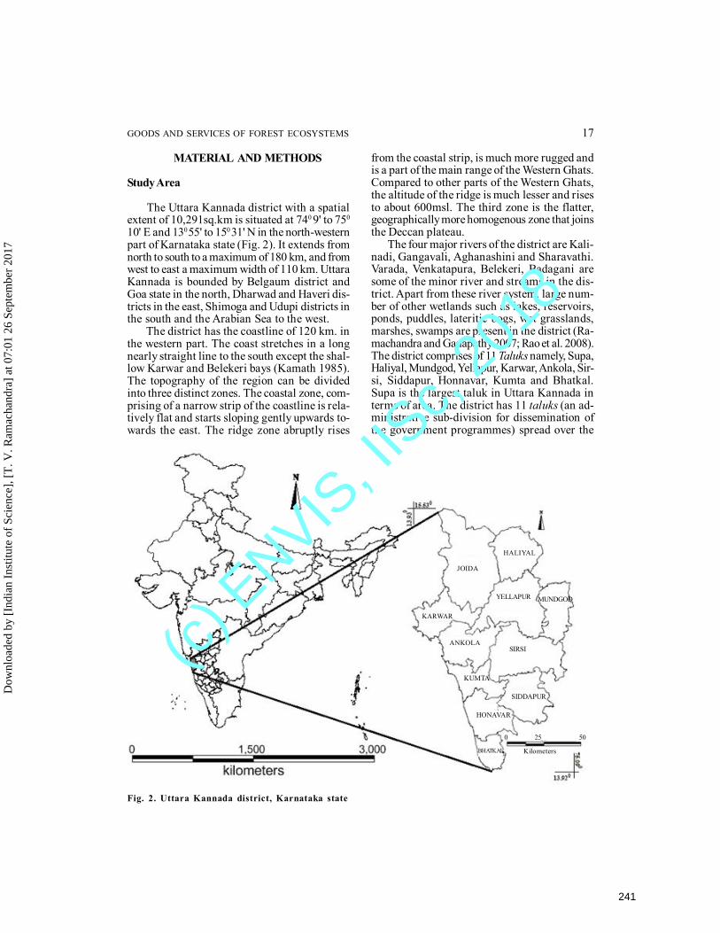
GOODS AND SERVICES OF FOREST ECOSYSTEMS 17
MATERIAL AND METHODS
Study Area
The Uttara Kannada district with a spatialextent of 10,291sq.km is situated at 740 9' to 750
10' E and 130 55' to 150 31' N in the north-westernpart of Karnataka state (Fig. 2). It extends fromnorth to south to a maximum of 180 km, and fromwest to east a maximum width of 110 km. UttaraKannada is bounded by Belgaum district andGoa state in the north, Dharwad and Haveri dis-tricts in the east, Shimoga and Udupi districts inthe south and the Arabian Sea to the west.
The district has the coastline of 120 km. inthe western part. The coast stretches in a longnearly straight line to the south except the shal-low Karwar and Belekeri bays (Kamath 1985).The topography of the region can be dividedinto three distinct zones. The coastal zone, com-prising of a narrow strip of the coastline is rela-tively flat and starts sloping gently upwards to-wards the east. The ridge zone abruptly rises
from the coastal strip, is much more rugged andis a part of the main range of the Western Ghats.Compared to other parts of the Western Ghats,the altitude of the ridge is much lesser and risesto about 600msl. The third zone is the flatter,geographically more homogenous zone that joinsthe Deccan plateau.
The four major rivers of the district are Kali-nadi, Gangavali, Aghanashini and Sharavathi.Varada, Venkatapura, Belekeri, Badagani aresome of the minor river and streams in the dis-trict. Apart from these river system, large num-ber of other wetlands such as lakes, reservoirs,ponds, puddles, lateritic bogs, wet grasslands,marshes, swamps are present in the district (Ra-machandra and Ganapathy 2007; Rao et al. 2008).The district comprises of 11 Taluks namely, Supa,Haliyal, Mundgod, Yellapur, Karwar, Ankola, Sir-si, Siddapur, Honnavar, Kumta and Bhatkal.Supa is the largest taluk in Uttara Kannada interms of area. The district has 11 taluks (an ad-ministrative sub-division for dissemination ofthe government programmes) spread over the
Fig. 2. Uttara Kannada district, Karnataka state
HALIYAL
JOIDA
YELLAPUR
KARWAR
ANKOLASIRSI
KUMTA
SIDDAPUR
HONAVAR
BHATKAL Kilometers
0 25 50
MUNDGOD
Dow
nloa
ded
by [
Indi
an I
nstit
ute
of S
cien
ce],
[T
. V. R
amac
hand
ra]
at 0
7:01
26
Sept
embe
r 20
17
241
(c) E
NVIS, I
ISc,
2018
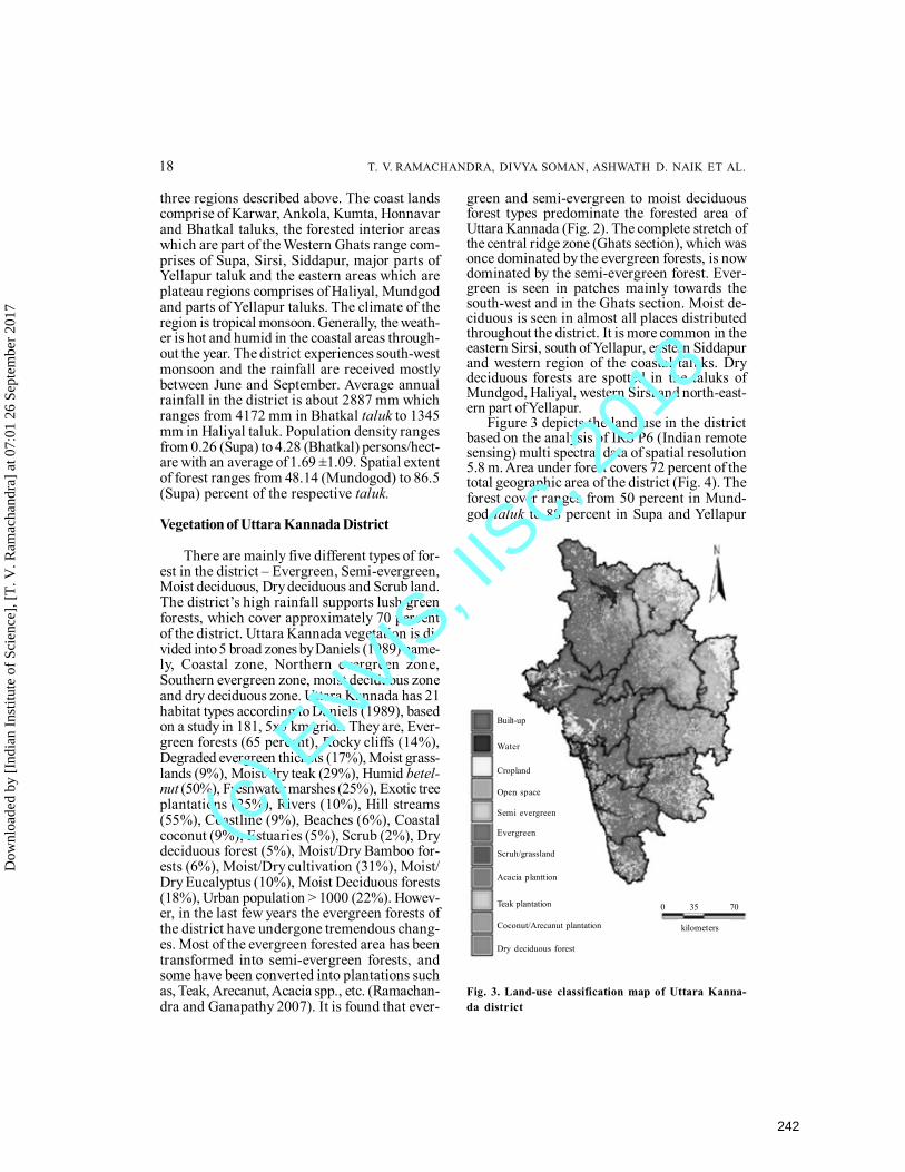
18 T. V. RAMACHANDRA, DIVYA SOMAN, ASHWATH D. NAIK ET AL.
three regions described above. The coast landscomprise of Karwar, Ankola, Kumta, Honnavarand Bhatkal taluks, the forested interior areaswhich are part of the Western Ghats range com-prises of Supa, Sirsi, Siddapur, major parts ofYellapur taluk and the eastern areas which areplateau regions comprises of Haliyal, Mundgodand parts of Yellapur taluks. The climate of theregion is tropical monsoon. Generally, the weath-er is hot and humid in the coastal areas through-out the year. The district experiences south-westmonsoon and the rainfall are received mostlybetween June and September. Average annualrainfall in the district is about 2887 mm whichranges from 4172 mm in Bhatkal taluk to 1345mm in Haliyal taluk. Population density rangesfrom 0.26 (Supa) to 4.28 (Bhatkal) persons/hect-are with an average of 1.69 ±1.09. Spatial extentof forest ranges from 48.14 (Mundogod) to 86.5(Supa) percent of the respective taluk.
Vegetation of Uttara Kannada District
There are mainly five different types of for-est in the district – Evergreen, Semi-evergreen,Moist deciduous, Dry deciduous and Scrub land.The district’s high rainfall supports lush greenforests, which cover approximately 70 percentof the district. Uttara Kannada vegetation is di-vided into 5 broad zones by Daniels (1989) name-ly, Coastal zone, Northern evergreen zone,Southern evergreen zone, moist deciduous zoneand dry deciduous zone. Uttara Kannada has 21habitat types according to Daniels (1989), basedon a study in 181, 5x5 km grids. They are, Ever-green forests (65 percent), Rocky cliffs (14%),Degraded evergreen thickets (17%), Moist grass-lands (9%), Moist/dry teak (29%), Humid betel-nut (50%), Freshwater marshes (25%), Exotic treeplantations (25%), Rivers (10%), Hill streams(55%), Coastline (9%), Beaches (6%), Coastalcoconut (9%), Estuaries (5%), Scrub (2%), Drydeciduous forest (5%), Moist/Dry Bamboo for-ests (6%), Moist/Dry cultivation (31%), Moist/Dry Eucalyptus (10%), Moist Deciduous forests(18%), Urban population > 1000 (22%). Howev-er, in the last few years the evergreen forests ofthe district have undergone tremendous chang-es. Most of the evergreen forested area has beentransformed into semi-evergreen forests, andsome have been converted into plantations suchas, Teak, Arecanut, Acacia spp., etc. (Ramachan-dra and Ganapathy 2007). It is found that ever-
green and semi-evergreen to moist deciduousforest types predominate the forested area ofUttara Kannada (Fig. 2). The complete stretch ofthe central ridge zone (Ghats section), which wasonce dominated by the evergreen forests, is nowdominated by the semi-evergreen forest. Ever-green is seen in patches mainly towards thesouth-west and in the Ghats section. Moist de-ciduous is seen in almost all places distributedthroughout the district. It is more common in theeastern Sirsi, south of Yellapur, eastern Siddapurand western region of the coastal taluks. Drydeciduous forests are spotted in the taluks ofMundgod, Haliyal, western Sirsi and north-east-ern part of Yellapur.
Figure 3 depicts the land use in the districtbased on the analysis of IRS P6 (Indian remotesensing) multi spectral data of spatial resolution5.8 m. Area under forest covers 72 percent of thetotal geographic area of the district (Fig. 4). Theforest cover ranges from 50 percent in Mund-god taluk to 88 percent in Supa and Yellapur
Fig. 3. Land-use classification map of Uttara Kanna-da district
Built-up
Water
Cropland
Open space
Semi evergreen
Evergreen
Scruh/grassland
Acacia planttion
Teak plantation
Coconut/Arecanut plantation
Dry deciduous forest
kilometers
0 35 70
Dow
nloa
ded
by [
Indi
an I
nstit
ute
of S
cien
ce],
[T
. V. R
amac
hand
ra]
at 0
7:01
26
Sept
embe
r 20
17
242
(c) E
NVIS, I
ISc,
2018
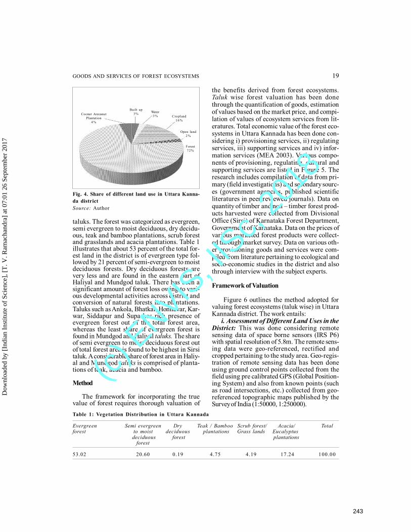
GOODS AND SERVICES OF FOREST ECOSYSTEMS 19
taluks. The forest was categorized as evergreen,semi evergreen to moist deciduous, dry decidu-ous, teak and bamboo plantations, scrub forestand grasslands and acacia plantations. Table 1illustrates that about 53 percent of the total for-est land in the district is of evergreen type fol-lowed by 21 percent of semi-evergreen to moistdeciduous forests. Dry deciduous forests arevery less and are found in the eastern part ofHaliyal and Mundgod taluk. There has been asignificant amount of forest loss owing to vari-ous developmental activities across district andconversion of natural forests into plantations.Taluks such as Ankola, Bhatkal, Honnavar, Kar-war, Siddapur and Supa has rich presence ofevergreen forest out of the total forest area,whereas the least share of evergreen forest isfound in Mundgod and Haliyal taluks. The shareof semi evergreen to moist deciduous forest outof total forest area is found to be highest in Sirsitaluk. A considerable share of forest area in Haliy-al and Mundgod taluks is comprised of planta-tions of teak, acacia and bamboo.
Method
The framework for incorporating the truevalue of forest requires thorough valuation of
the benefits derived from forest ecosystems.Taluk wise forest valuation has been donethrough the quantification of goods, estimationof values based on the market price, and compi-lation of values of ecosystem services from lit-eratures. Total economic value of the forest eco-systems in Uttara Kannada has been done con-sidering i) provisioning services, ii) regulatingservices, iii) supporting services and iv) infor-mation services (MEA 2003). Various compo-nents of provisioning, regulating, cultural andsupporting services are listed in Figure 5. Theresearch includes compilation of data from pri-mary (field investigations) and secondary sourc-es (government agencies, published scientificliteratures in peer reviewed journals). Data onquantity of timber and non – timber forest prod-ucts harvested were collected from DivisionalOffice (Sirsi) of Karnataka Forest Department,Government of Karnataka. Data on the prices ofvarious marketed forest products were collect-ed through market survey. Data on various oth-er provisioning goods and services were com-piled from literature pertaining to ecological andsocio-economic studies in the district and alsothrough interview with the subject experts.
Framework of Valuation
Figure 6 outlines the method adopted forvaluing forest ecosystems (taluk wise) in UttaraKannada district. The work entails:
i. Assessment of Different Land Uses in theDistrict: This was done considering remotesensing data of space borne sensors (IRS P6)with spatial resolution of 5.8m. The remote sens-ing data were geo-referenced, rectified andcropped pertaining to the study area. Geo-regis-tration of remote sensing data has been doneusing ground control points collected from thefield using pre calibrated GPS (Global Position-ing System) and also from known points (suchas road intersections, etc.) collected from geo-referenced topographic maps published by theSurvey of India (1:50000, 1:250000).
Fig. 4. Share of different land use in Uttara Kanna-da districtSource: Author
Built up3% Water
3% Cropland16%
Open land2%
Forest72%
Cocnut ArecanutPlantation
4%
Table 1: Vegetation Distribution in Uttara Kannada
Evergreen Semi evergreen Dry Teak / Bamboo Scrub forest/ Acacia/ Totalforest to moist deciduous plantations Grass lands Eucalyptus
deciduous forest plantationsforest
53.02 20.60 0.19 4.75 4.19 17.24 100.00
Dow
nloa
ded
by [
Indi
an I
nstit
ute
of S
cien
ce],
[T
. V. R
amac
hand
ra]
at 0
7:01
26
Sept
embe
r 20
17
243
(c) E
NVIS, I
ISc,
2018
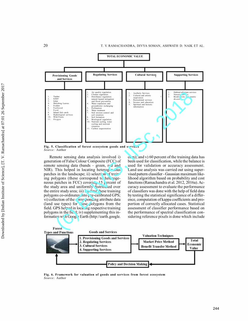
20 T. V. RAMACHANDRA, DIVYA SOMAN, ASHWATH D. NAIK ET AL.
Remote sensing data analysis involved i)generation of False Colour Composite (FCC) ofremote sensing data (bands – green, red andNIR). This helped in locating heterogeneouspatches in the landscape; ii) selection of train-ing polygons (these correspond to heteroge-neous patches in FCC) covering 15 percent ofthe study area and uniformly distributed overthe entire study area; iii) loading these trainingpolygons co-ordinates into pre-calibrated GPS;vi) collection of the corresponding attribute data(land use types) for these polygons from thefield. GPS helped in locating respective trainingpolygons in the field; iv) supplementing this in-formation with Google Earth (http://earth.google.
com); and v) 60 percent of the training data hasbeen used for classification, while the balance isused for validation or accuracy assessment.Land use analysis was carried out using super-vised pattern classifier - Gaussian maximum like-lihood algorithm based on probability and costfunctions (Ramachandra et al. 2012, 2016a). Ac-curacy assessment to evaluate the performanceof classifiers was done with the help of field databy testing the statistical significance of a differ-ence, computation of kappa coefficients and pro-portion of correctly allocated cases. Statisticalassessment of classifier performance based onthe performance of spectral classification con-sidering reference pixels is done which include
Fig. 5. Classification of forest ecosystem goods and servicesSource: Author
TOTAL ECONOMIC VALUE
Provisioning Goodsand Services
Regulating Services Cultural Services Supporting Services
1 . Timber2 . NTFP3 . Litter4 . Mulching Leaves5 . Fodder6 . Fuelwood7 . Food8 . Inland fish catch9 . Hydrological services10 . Wild Fruits11 . Oxygen
1 . Air quality regulation2 . Climate regulation3 . Distribance regulation
natural hazard mitigationand flood prevention
4 . Water repulation andgroundwater recharging
5 . Pollination6 . Water treatment7 . Soil erosion control and
soil retention8 . Soil formation9 . Biiological regulation10 . Nutrient cycling, water
cycling and nutrientretention
11 . Carbon sequestration
1 . Aesthetic Services2 . Cultural and artistic
inspiration3 . Recreational services4 . Science and education5 . Spiritual and historic
information
1 . Habitat/refugium services2 . Nursery services3 . Biodiversity and genetic
diversi ty
Fig. 6. Framework for valuation of goods and services from forest ecosystemSource: Author
Dow
nloa
ded
by [
Indi
an I
nstit
ute
of S
cien
ce],
[T
. V. R
amac
hand
ra]
at 0
7:01
26
Sept
embe
r 20
17
244
(c) E
NVIS, I
ISc,
2018
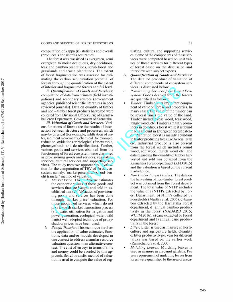
GOODS AND SERVICES OF FOREST ECOSYSTEMS 21
computation of kappa () statistics and overall(producer’s and user’s) accuracies.
The forest was classified as evergreen, semievergreen to moist deciduous, dry deciduous,teak and bamboo plantations, scrub forest andgrasslands and acacia plantations. The extentof forest fragmentation was assessed for esti-mating the carbon sequestration potential offorests through the quantification of the extentof interior and fragmented forests at taluk level.
ii. Quantification of Goods and Services:compilation of data from primary (field investi-gations) and secondary sources (governmentagencies, published scientific literatures in peerreviewed journals). Data on quantity of timberand non – timber forest products harvested werecollected from Divisional Office (Sirsi) of Karnata-ka Forest Department, Government of Karnataka.
iii. Valuation of Goods and Services: Vari-ous functions of forests are the results of inter-action between structure and processes, whichmay be physical (for example, infiltration of wa-ter, sediment movement), chemical (for example,reduction, oxidation) or biological (for example,photosynthesis and de-nitrification). Further,various goods and services obtained from thefunctioning of forest ecosystem were classifiedas provisioning goods and services, regulatingservices, cultural services and supporting ser-vices. The study uses two approaches of valua-tion for the computation of TEV of forest eco-system, namely: ‘market price’ method and ‘ben-efit transfer’ method of valuation.
a. Market Price: This technique estimatesthe economic values of those goods andservices that are bought and sold in es-tablished markets. Valuation of provision-ing goods and services has been donethrough ‘market price’ valuation. Forthose goods and services which do notpass through market transaction process(viz. water utilization for irrigation andpower generation, ecological water, wildfruits) well adopted technique of proxy/shadow prices have been used.
b. Benefit Transfer: This technique involvesthe application of value estimates, func-tions, data and/or models developed inone context to address a similar resourcevaluation question in an alternative con-text. The cost of surveys in terms of timeand money could be avoided by this ap-proach. Benefit transfer method of valua-tion is used to compute the value of reg-
ulating, cultural and supporting servic-es. Some of the components of these ser-vices were computed based on unit val-ues of those services for different typesof forest based on the discussion andinterview with subject experts.
iv. Quantification of Goods and Services:The detailed procedure of valuation ofdifferent components of ecosystem ser-vices is discussed below:
a. Provisioning Services from Forest Eco-system: Goods derived from the forestsare quantified as follows:
• Timber: Timber is an important compo-nent of value on forestland properties. Inmany cases, the value of the timber canbe several times the value of the land.Timber includes rose wood, teak wood,jungle wood, etc. Timber is mainly prom-inent in deciduous forest while it is foundin less amount in Evergreen forest patch-es. Plantation forest is mainly abundantin timber producing trees like Acacia, Teaketc. Industrial produce is also presentfrom the forest which includes roundwood, soft wood, match wood etc. Thedata regarding the quantity of timber har-vested and sold was obtained from theKarnataka Forest department (KFD 2015)and the valuation is based on the currentmarket price.
• Non Timber Forest Product: The data onthe harvesting of non-timber forest prod-uct was obtained from the Forest depart-ment. The total value of NTFP includesthe value of a) NTFPs extracted by For-est Department, b) NTFPs collected byhouseholds (Murthy et al. 2005), c) bam-boo extracted by the Karnataka Forestdepartment, d) annual bamboo produc-tivity in the forest (NABARD 2015;WCPM 2016), e) cane extracted by Forestdepartment and f) annual cane produc-tivity in the forest .
• Litter: Litter is used as manure in horti-culture and agriculture fields. Quantityof litter productivity per year for differenttaluks was based on the earlier work(Ramachandra et al. 2000).
• Mulching Leaves: Mulching leaves isused as manure in arecanut gardens. Peryear requirement of mulching leaves fromforest were quantified by the area of areca-
Dow
nloa
ded
by [
Indi
an I
nstit
ute
of S
cien
ce],
[T
. V. R
amac
hand
ra]
at 0
7:01
26
Sept
embe
r 20
17
245
(c) E
NVIS, I
ISc,
2018
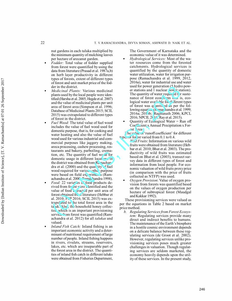
22 T. V. RAMACHANDRA, DIVYA SOMAN, ASHWATH D. NAIK ET AL.
nut gardens in each taluka multiplied bythe minimum quantity of mulching leavesper hectare of arecanut garden.
• Fodder: Total value of fodder suppliedfrom forest were quantified by using thedata from literature (Prasad et al. 1987a,b)on herb layer productivity in differenttypes of forests, extent of different typesof forest and unit market price of the fod-der in the district.
• Medicinal Plants: Various medicinalplants used by the local people were iden-tified (Harsha et al. 2005; Hegde et al. 2007)and the value of medicinal plants per unitarea of forest area (Simpson et al. 1996;Database of Medicinal Plants 2015; SCIL2015) was extrapolated to different typesof forest in the district.
• Fuel Wood: The total value of fuel woodincludes the value of fuel wood used fordomestic purpose, that is, for cooking andwater heating and also the value of fuelwood used for various industrial and com-mercial purposes like jaggery making,areca processing, cashew processing, res-taurants and bakery, parboiling, crema-tion, etc. The quantity of fuel wood fordomestic usage in different locations ofthe district was obtained from Ramachan-dra et al. (2000) and the quantity of fuelwood required for various other purposewere based on field experiments (Ram-achandra et al. 2000; Ramachandra 1998).
• Food: 22 varieties of food products de-rived from forest were identified and thevalue of food extracted per unit area offorest obtained from literature (Hebbar etal. 2010; PSP 2016; SCIL 2015) was ex-trapolated to the total forest area in thetaluk. Also, the household honey collec-tion which is an important provisioningservice from forest was quantified (Ram-achandra et al. 2012) for all talukas andvalued.
• Inland Fish Catch: Inland fishing is animportant economic activity and a deter-minant of nutritional requirement of largenumber of people. Inland fishing happensin rivers, rivulets, streams, reservoirs,lakes, etc. which are inseparable part ofthe forest area in the district. The quanti-ties of inland fish catch in different talukswere obtained from Fisheries Department,
The Government of Karnataka and theeconomic value of it was determined.
• Hydrological Services: Most of the wa-ter resources come from the forestedcatchments. Hydrological services isquantified by the quantity of domesticwater utilization, water for irrigation pur-pose (Ramachandra et al. 1999, 2012,2016a), water for industrial use and waterused for power generation (5 hydro pow-er stations and 1 nuclear power station).The quantity of water required for suste-nance of forest ecosystem that is, eco-logical water available for different typesof forest was quantified as per the fol-lowing equation (Ramachandra et al. 1999;2016a; 2016b; Raghunath 2006; KPCL2016; NPCIL 2016; Ray et al. 2015).
• Quantity of Ecological Water = Run offCoefficient x Annual Precipitation x For-est Area
The value of ‘runoff coefficient’ for differenttypes of forest varied from 0.1 to 0.4.
• Wild Fruits: Information on various wildfruits were obtained from literature (Heb-bar et al. 2010; Bhat et al. 2003). The pro-ductivity of wild fruits was estimatedbased on Bhat et al. (2003), transect sur-vey data in different types of forest andinformation from local people. For eco-nomic valuation of wild fruits proxy price(in comparison with the price of fruitscollected as NTFP) was used.
• Oxygen Provision: Value of oxygen pro-vision from forests was quantified basedon the values of oxygen production perhectare of subtropical forest (Maudgaland Kakkar 1992).
These provisioning services were valued asper the equations in Table 2 based on marketprice method.
b. Regulating Services from Forest Ecosys-tem: Regulating services provide manydirect and indirect benefits to humans.The maintenance of the Earth’s biospherein a hostile cosmic environment dependson a delicate balance between these reg-ulating services (de Groot et al. 2002).However, regulating services unlike pro-visioning services poses much greaterchallenges in valuation. Though regulat-ing services are seldom marketed, theeconomy heavily depends upon the util-ity of these services. In the present study,
Dow
nloa
ded
by [
Indi
an I
nstit
ute
of S
cien
ce],
[T
. V. R
amac
hand
ra]
at 0
7:01
26
Sept
embe
r 20
17
246
(c) E
NVIS, I
ISc,
2018
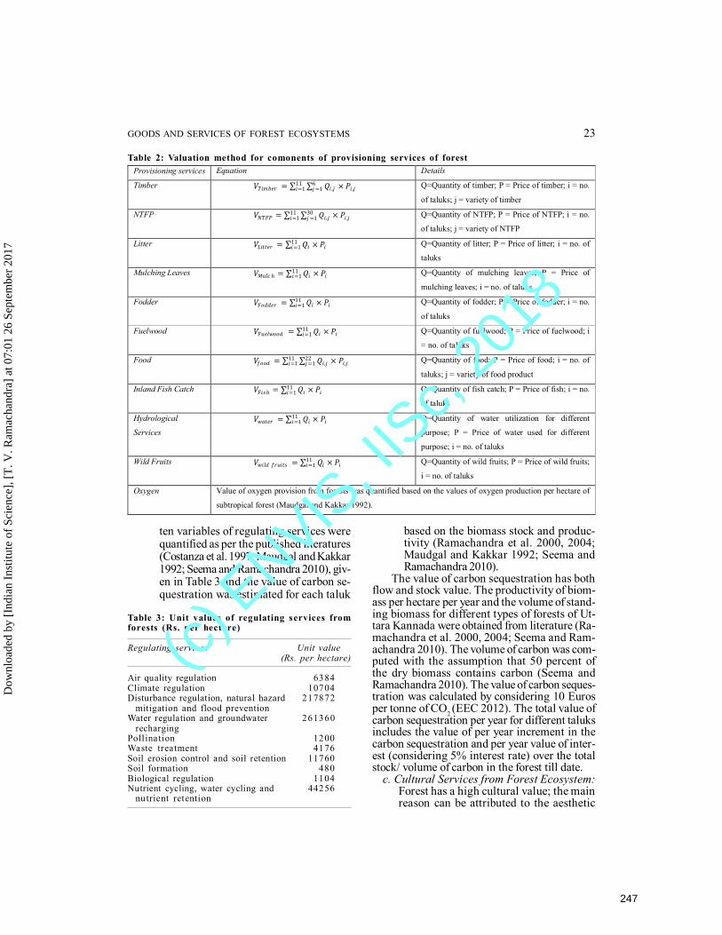
GOODS AND SERVICES OF FOREST ECOSYSTEMS 23
ten variables of regulating services werequantified as per the published literatures(Costanza et al. 1997; Maudgal and Kakkar1992; Seema and Ramachandra 2010), giv-en in Table 3 and the value of carbon se-questration was estimated for each taluk
based on the biomass stock and produc-tivity (Ramachandra et al. 2000, 2004;Maudgal and Kakkar 1992; Seema andRamachandra 2010).
The value of carbon sequestration has bothflow and stock value. The productivity of biom-ass per hectare per year and the volume of stand-ing biomass for different types of forests of Ut-tara Kannada were obtained from literature (Ra-machandra et al. 2000, 2004; Seema and Ram-achandra 2010). The volume of carbon was com-puted with the assumption that 50 percent ofthe dry biomass contains carbon (Seema andRamachandra 2010). The value of carbon seques-tration was calculated by considering 10 Eurosper tonne of CO2 (EEC 2012). The total value ofcarbon sequestration per year for different taluksincludes the value of per year increment in thecarbon sequestration and per year value of inter-est (considering 5% interest rate) over the totalstock/ volume of carbon in the forest till date.
c. Cultural Services from Forest Ecosystem:Forest has a high cultural value; the mainreason can be attributed to the aesthetic
Provisioning services Equation Details
Timber 푉푇푖푚푏푒푟 = ∑ ∑ 푄푖 ,푗 × 푃푖,푗6푗=1
11푖=1 Q=Quantity of timber; P = Price of timber; i = no.
of taluks; j = variety of timber
NTFP 푉푁푇퐹푃 = ∑ ∑ 푄푖,푗 × 푃푖 ,푗30푗=1
11푖=1 Q=Quantity of NTFP; P = Price of NTFP; i = no.
of taluks; j = variety of NTFP
Litter 푉퐿푖푡푡푒푟 = ∑ 푄푖 × 푃푖11푖=1 Q=Quantity of litter; P = Price of litter; i = no. of
taluks
Mulching Leaves 푉푀푢푙푐 ℎ = ∑ 푄푖 × 푃푖11푖=1 Q=Quantity of mulching leaves; P = Price of
mulching leaves; i = no. of taluks
Fodder 푉퐹표푑푑푒푟 = ∑ 푄푖 × 푃푖11푖=1 Q=Quantity of fodder; P = Price of fodder; i = no.
of taluks
Fuelwood 푉퐹푢푒푙푤표표푑 = ∑ 푄푖 × 푃푖11푖=1 Q=Quantity of fuelwood; P = Price of fuelwood; i
= no. of taluks
Food 푉푓표표푑 = ∑ ∑ 푄푖,푗 × 푃푖,푗22푗=1
11푖=1 Q=Quantity of food; P = Price of food; i = no. of
taluks; j = variety of food product
Inland Fish Catch 푉퐹푖푠ℎ = ∑ 푄푖 × 푃푖11푖=1 Q=Quantity of fish catch; P = Price of fish; i = no.
of taluks
Hydrological
Services 푉푤푎푡푒푟 = ∑ 푄푖 × 푃푖11
푖=1 Q=Quantity of water utilization for different
purpose; P = Price of water used for different
purpose; i = no. of taluks
Wild Fruits 푉푤푖푙푑 푓푟푢푖푡푠 = ∑ 푄푖 × 푃푖11푖=1 Q=Quantity of wild fruits; P = Price of wild fruits;
i = no. of taluks
Oxygen Value of oxygen provision from forests was quantified based on the values of oxygen production per hectare of
subtropical forest (Maudgal and Kakkar 1992).
Table 2: Valuation method for comonents of provisioning services of forest
Table 3: Unit values of regulating services fromforests (Rs. per hectare)
Regulating services Unit value(Rs. per hectare)
Air quality regulation 6384Climate regulation 10704Disturbance regulation, natural hazard 217872
mitigation and flood preventionWater regulation and groundwater 261360
rechargingPollination 1200Waste treatment 4176Soil erosion control and soil retention 11760Soil formation 480Biological regulation 1104Nutrient cycling, water cycling and 44256
nutrient retention
Dow
nloa
ded
by [
Indi
an I
nstit
ute
of S
cien
ce],
[T
. V. R
amac
hand
ra]
at 0
7:01
26
Sept
embe
r 20
17
247
(c) E
NVIS, I
ISc,
2018
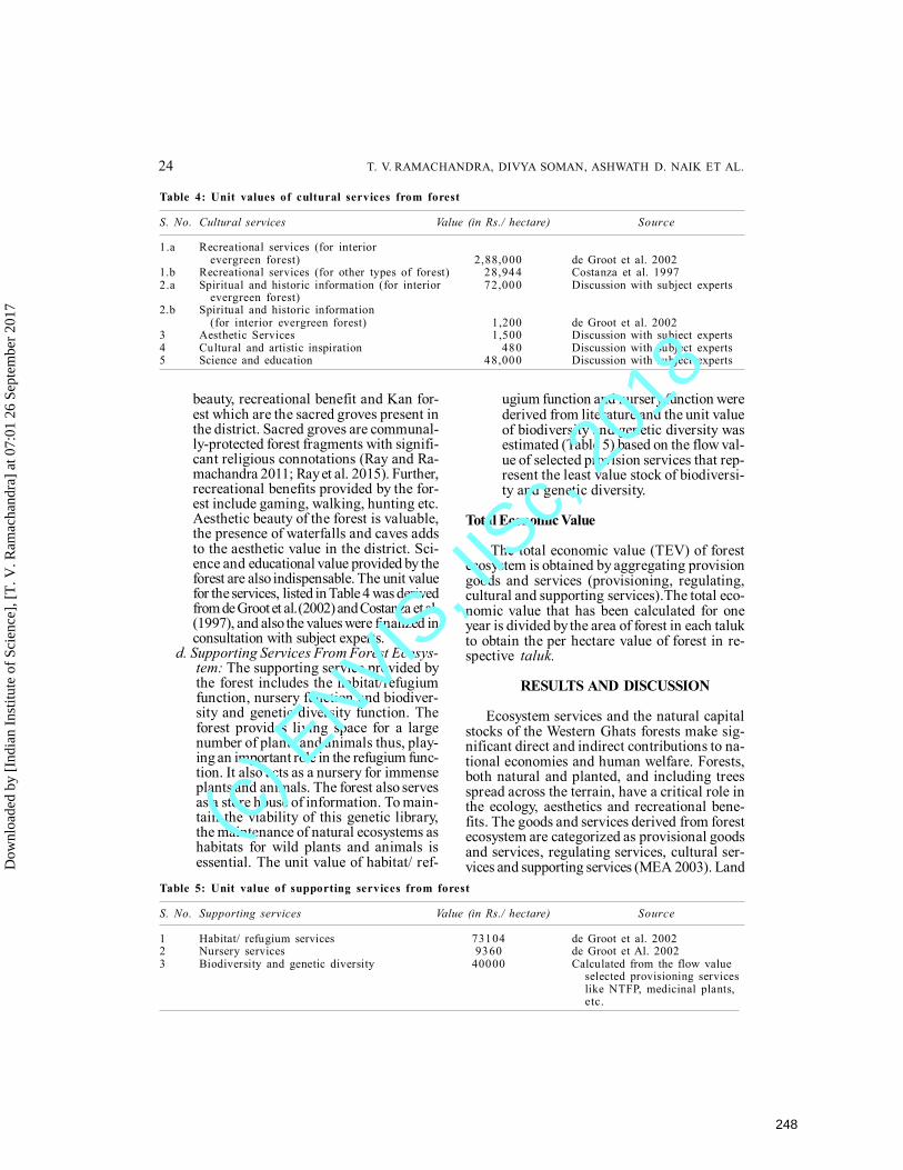
24 T. V. RAMACHANDRA, DIVYA SOMAN, ASHWATH D. NAIK ET AL.
beauty, recreational benefit and Kan for-est which are the sacred groves present inthe district. Sacred groves are communal-ly-protected forest fragments with signifi-cant religious connotations (Ray and Ra-machandra 2011; Ray et al. 2015). Further,recreational benefits provided by the for-est include gaming, walking, hunting etc.Aesthetic beauty of the forest is valuable,the presence of waterfalls and caves addsto the aesthetic value in the district. Sci-ence and educational value provided by theforest are also indispensable. The unit valuefor the services, listed in Table 4 was derivedfrom de Groot et al. (2002) and Costanza et al.(1997), and also the values were finalized inconsultation with subject experts.
d. Supporting Services From Forest Ecosys-tem: The supporting service provided bythe forest includes the habitat/refugiumfunction, nursery function and biodiver-sity and genetic diversity function. Theforest provides living space for a largenumber of plants and animals thus, play-ing an important role in the refugium func-tion. It also acts as a nursery for immenseplants and animals. The forest also servesas a store house of information. To main-tain the viability of this genetic library,the maintenance of natural ecosystems ashabitats for wild plants and animals isessential. The unit value of habitat/ ref-
ugium function and nursery function werederived from literature and the unit valueof biodiversity and genetic diversity wasestimated (Table 5) based on the flow val-ue of selected provision services that rep-resent the least value stock of biodiversi-ty and genetic diversity.
Total Economic Value
The total economic value (TEV) of forestecosystem is obtained by aggregating provisiongoods and services (provisioning, regulating,cultural and supporting services).The total eco-nomic value that has been calculated for oneyear is divided by the area of forest in each talukto obtain the per hectare value of forest in re-spective taluk.
RESULTS AND DISCUSSION
Ecosystem services and the natural capitalstocks of the Western Ghats forests make sig-nificant direct and indirect contributions to na-tional economies and human welfare. Forests,both natural and planted, and including treesspread across the terrain, have a critical role inthe ecology, aesthetics and recreational bene-fits. The goods and services derived from forestecosystem are categorized as provisional goodsand services, regulating services, cultural ser-vices and supporting services (MEA 2003). Land
Table 4: Unit values of cultural services from forest
S. No. Cultural services Value (in Rs./ hectare) Source
1.a Recreational services (for interiorevergreen forest) 2,88,000 de Groot et al. 2002
1.b Recreational services (for other types of forest) 28,944 Costanza et al. 19972.a Spiritual and historic information (for interior 72,000 Discussion with subject experts
evergreen forest)2.b Spiritual and historic information
(for interior evergreen forest) 1,200 de Groot et al. 20023 Aesthetic Services 1,500 Discussion with subject experts4 Cultural and artistic inspiration 480 Discussion with subject experts5 Science and education 48,000 Discussion with subject experts
Table 5: Unit value of supporting services from forest
S. No. Supporting services Value (in Rs./ hectare) Source
1 Habitat/ refugium services 73104 de Groot et al. 20022 Nursery services 9360 de Groot et Al. 20023 Biodiversity and genetic diversity 40000 Calculated from the flow value
selected provisioning serviceslike NTFP, medicinal plants,etc.
Dow
nloa
ded
by [
Indi
an I
nstit
ute
of S
cien
ce],
[T
. V. R
amac
hand
ra]
at 0
7:01
26
Sept
embe
r 20
17
248
(c) E
NVIS, I
ISc,
2018
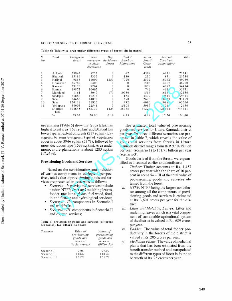
GOODS AND SERVICES OF FOREST ECOSYSTEMS 25
use analysis (Table 6) show that Supa taluk hashighest forest area (1635 sq.km) and Bhatkal haslowest spatial extent of forests (217 sq.km). Ev-ergreen to semi evergreen type of vegetationcover is about 3946 sq.km (53 %), followed bymoist deciduous type (1533 sq.km). Area undermonoculture plantations is about 1283 sq.km(17.24 %).
Provisioning Goods and Services
Based on the consideration and inclusionof various components in ecological perspec-tives, total value of provisioning goods and ser-vices are presented in scenarios as follows:
• Scenario - I: provisional services includetimber, NTFP, litter and mulching leaves,fodder, medicinal plants, fuel wood, food,inland fishing and hydrological services;
• Scenario - II: components in Scenario-Iand wild fruits;
• Scenario - III: components in Scenario-IIand oxygen services;
The estimated total value of provisioninggoods and services for Uttara Kannada districtper year for three different scenarios are pre-sented in Table 7, which reveals the value ofgoods and services from forests in UttaraKannada district ranges from INR 97.07 billionper year (scenario 1) to 151.71 billion per year(scenario 3).
Goods derived from the forests were quan-tified as discussed earlier and details are:
i. Timber: Timber accounts to Rs. 1,457crores per year with the share of 10 per-cent in scenario – III of the total value ofprovisioning goods and services ob-tained from the forest.
ii. NTFP: NTFP being the largest contribu-tor among all the components of provi-sioning goods and services is estimatedat Rs. 3,601 crores per year for the dis-trict.
iii. Litter and Mulching Leaves: Litter andmulching leaves which is a vital compo-nent of sustainable agricultural systemof the district is valued at Rs. 689 croresper year.
iv. Fodder: The value of total fodder pro-ductivity in the forests of the district isvalued at Rs. 205 crores per year.
v. Medicinal Plants: The value of medicinalplants that has been estimated from thebenefit transfer method and extrapolatedto the different types of forest is found tobe worth of Rs. 25 crores per year.
Table 6: Talukwise area under different types of forest (in hectares)
S. Taluk Evergreen Semi Dry Teak / Scrub Acacia/ TotalNo. forest evergreen deciduous Bam boo forest/ Eucalyptu
to Moist forest Plantations Grass splantationsdeciduous lands
1 Ankola 53943 8227 0 6 2 4598 6911 737412 Bhatkal 15189 5335 0 130 230 851 217343 Haliyal 9853 11609 1253 7720 2532 16062 490304 Honnavar 36782 6403 0 0 1508 4007 487005 Karwar 39176 9264 0 0 1878 4097 544146 Kumta 19873 10697 0 0 746 4615 359317 Mundgod 1161 3047 171 10080 1554 16144 321568 Siddapur 35882 10214 0 124 3479 9615 593159 Sirsi 24666 44070 0 1670 2620 20133 931591 0 Supa 124118 21923 0 492 6090 10882 1635041 1 Yellapura 34003 22541 0 15108 5987 35017 112656
District 394645 153330 1424 35385 31223 128334 744341 Total% 53.02 20.60 0.19 4.75 4.19 17.24 100.00
Table 7: Provisioning goods and services (differentscenarios) for Uttara Kannada
Scenario Value of Values ofprovisioning provisioninggoods and goods and
services services(in Rs. crores) (Billion Rs)
Scenario I 9707 97.07Scenario II 11842 118.42Scenario III 15171 151.71
Dow
nloa
ded
by [
Indi
an I
nstit
ute
of S
cien
ce],
[T
. V. R
amac
hand
ra]
at 0
7:01
26
Sept
embe
r 20
17
249
(c) E
NVIS, I
ISc,
2018
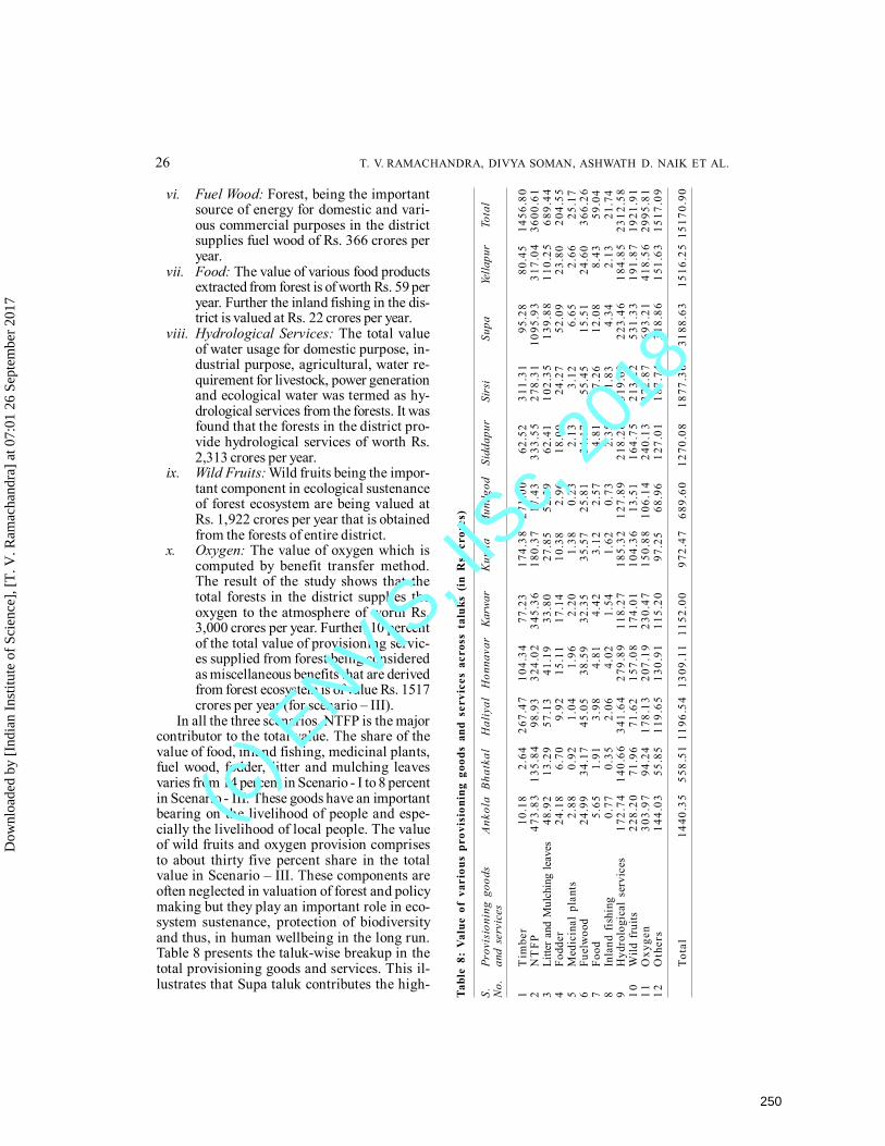
26 T. V. RAMACHANDRA, DIVYA SOMAN, ASHWATH D. NAIK ET AL.
vi. Fuel Wood: Forest, being the importantsource of energy for domestic and vari-ous commercial purposes in the districtsupplies fuel wood of Rs. 366 crores peryear.
vii. Food: The value of various food productsextracted from forest is of worth Rs. 59 peryear. Further the inland fishing in the dis-trict is valued at Rs. 22 crores per year.
viii. Hydrological Services: The total valueof water usage for domestic purpose, in-dustrial purpose, agricultural, water re-quirement for livestock, power generationand ecological water was termed as hy-drological services from the forests. It wasfound that the forests in the district pro-vide hydrological services of worth Rs.2,313 crores per year.
ix. Wild Fruits: Wild fruits being the impor-tant component in ecological sustenanceof forest ecosystem are being valued atRs. 1,922 crores per year that is obtainedfrom the forests of entire district.
x. Oxygen: The value of oxygen which iscomputed by benefit transfer method.The result of the study shows that thetotal forests in the district supplies theoxygen to the atmosphere of worth Rs.3,000 crores per year. Further, 10 percentof the total value of provisioning servic-es supplied from forest being consideredas miscellaneous benefits that are derivedfrom forest ecosystem is of value Rs. 1517crores per year (for scenario – III).
In all the three scenarios, NTFP is the majorcontributor to the total value. The share of thevalue of food, inland fishing, medicinal plants,fuel wood, fodder, litter and mulching leavesvaries from 14 percent in Scenario - I to 8 percentin Scenario - III. These goods have an importantbearing on the livelihood of people and espe-cially the livelihood of local people. The valueof wild fruits and oxygen provision comprisesto about thirty five percent share in the totalvalue in Scenario – III. These components areoften neglected in valuation of forest and policymaking but they play an important role in eco-system sustenance, protection of biodiversityand thus, in human wellbeing in the long run.Table 8 presents the taluk-wise breakup in thetotal provisioning goods and services. This il-lustrates that Supa taluk contributes the high-
Tabl
e 8:
Val
ue o
f va
riou
s pr
ovis
ioni
ng g
oods
and
ser
vice
s ac
ross
tal
uks
(in
Rs.
cro
res)
S.Pr
ovis
ioni
ng g
oods
Ank
ola
Bha
tkal
Hal
iyal
Hon
nava
r K
arw
ar K
umta
M
undg
od
Sidd
apur
Si
rsi
Su
pa
Yel
lapu
rTo
tal
No.
and
serv
ices
1T
imbe
r10
.18
2.64
267.
4710
4.34
77.2
317
4.38
271.
0062
.52
311.
3195
.28
80.4
514
56.8
02
NT
FP47
3.83
135.
8498
.93
324.
0234
5.36
180.
3717
.43
333.
5527
8.31
1095
.93
317.
0436
00.6
13
Litte
r an
d M
ulch
ing
leav
es48
.92
13.2
957
.13
41.1
933
.80
27.8
552
.39
62.4
110
2.35
139.
8811
0.25
689.
444
Fodd
er24
.18
6.70
9.92
15.1
117
.14
10.3
82.
9618
.00
24.2
752
.09
23.8
020
4.55
5M
edic
inal
pla
nts
2.88
0.92
1.04
1.96
2.20
1.38
0.23
2.13
3.12
6.65
2.66
25.1
76
Fuel
woo
d24
.99
34.1
745
.05
38.5
932
.35
35.5
725
.81
34.1
755
.45
15.5
124
.60
366.
267
Food
5.65
1.91
3.98
4.81
4.42
3.12
2.57
4.81
7.26
12.0
88.
4359
.04
8In
land
fis
hing
0.77
0.35
2.06
4.02
1.54
1.62
0.73
2.35
1.83
4.34
2.13
21.7
49
Hyd
rolo
gica
l se
rvic
es17
2.74
140.
6634
1.64
279.
8911
8.27
185.
3212
7.89
218.
2631
9.62
223.
4618
4.85
2312
.58
10W
ild f
ruits
228.
2071
.96
71.6
215
7.08
174.
0110
4.36
13.5
116
4.75
213.
2253
1.33
191.
8719
21.9
111
Oxy
gen
303.
9794
.24
178.
1320
7.19
230.
4715
0.88
106.
1424
0.13
372.
8769
3.21
418.
5629
95.8
112
Oth
ers
144.
0355
.85
119.
6513
0.91
115.
2097
.25
68.9
612
7.01
187.
7431
8.86
151.
6315
17.0
9
Tota
l14
40.3
555
8.51
1196
.54
1309
.11
1152
.00
972.
4768
9.60
1270
.08
1877
.36
3188
.63
1516
.25
1517
0.90
Dow
nloa
ded
by [
Indi
an I
nstit
ute
of S
cien
ce],
[T
. V. R
amac
hand
ra]
at 0
7:01
26
Sept
embe
r 20
17
250
(c) E
NVIS, I
ISc,
2018
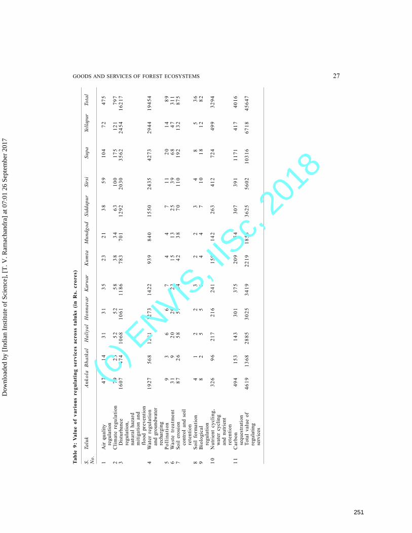
GOODS AND SERVICES OF FOREST ECOSYSTEMS 27Ta
ble
9: V
alue
of
vari
ous
regu
lati
ng s
ervi
ces
acro
ss t
aluk
s (i
n R
s. c
rore
s)
S.Ta
luk
Ank
ola
Bha
tkal
Hal
iyal
Hon
nava
r K
arw
ar K
umta
M
undg
od
Sidd
apur
Si
rsi
Su
pa
Yel
lapu
rTo
tal
No.
1A
ir q
ualit
y47
1431
3135
2321
3859
104
7247
5
regu
latio
n2
Clim
ate
regu
latio
n79
2352
5258
3834
6310
017
512
179
73
D
istu
rban
ce16
0747
410
6810
6111
8678
370
112
9220
3035
6224
5416
217
re
gula
tion,
na
tura
l ha
zard
m
itiga
tion
and
fl
ood
prev
entio
n4
Wat
er r
egul
atio
n19
2756
812
8112
7314
2293
984
015
5024
3542
7329
4419
454
an
d gr
ound
wat
er
rech
argi
ng5
Poll
inat
ion
93
66
74
47
1120
1489
6W
aste
tre
atm
ent
319
2020
2315
1325
3968
4731
17
Soil
eros
ion
8726
5857
6442
3870
110
192
132
875
co
ntro
l an
d so
il
rete
ntio
n8
Soil
for
mat
ion
41
22
32
23
48
536
9B
iolo
gica
l8
25
56
44
710
1812
82
regu
latio
n10
Nut
rien
t cy
clin
g,32
696
217
216
241
159
142
263
412
724
499
3294
w
ater
cyc
ling
an
d nu
trie
nt
rete
ntio
n11
Car
bon
494
153
143
301
375
209
5430
739
111
7141
740
16
sequ
estr
atio
n
Tota
l va
lue
of46
1913
6828
8530
2534
1922
1918
5336
2556
0210
316
6718
4564
7
regu
latin
g
serv
ices
Dow
nloa
ded
by [
Indi
an I
nstit
ute
of S
cien
ce],
[T
. V. R
amac
hand
ra]
at 0
7:01
26
Sept
embe
r 20
17
251
(c) E
NVIS, I
ISc,
2018
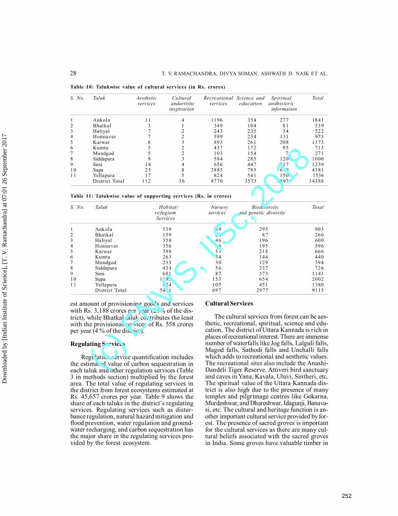
28 T. V. RAMACHANDRA, DIVYA SOMAN, ASHWATH D. NAIK ET AL.
est amount of provisioning goods and serviceswith Rs. 3,188 crores per year (21% of the dis-trict), while Bhatkal taluk contributes the leastwith the provisional services of Rs. 558 croresper year (4 % of the district).
Regulating Services
Regulation service quantification includesthe estimated value of carbon sequestration ineach taluk and other regulation services (Table3 in methods section) multiplied by the forestarea. The total value of regulating services inthe district from forest ecosystems estimated atRs. 45,657 crores per year. Table 9 shows theshare of each taluks in the district’s regulatingservices. Regulating services such as distur-bance regulation, natural hazard mitigation andflood prevention, water regulation and ground-water recharging, and carbon sequestration hasthe major share in the regulating services pro-vided by the forest ecosystem.
Cultural Services
The cultural services from forest can be aes-thetic, recreational, spiritual, science and edu-cation. The district of Uttara Kannada is rich inplaces of recreational interest. There are immensenumber of waterfalls like Jog falls, Lalguli falls,Magod falls, Sathodi falls and Unchalli fallswhich adds to recreational and aesthetic values.The recreational sites also include the Anashi-Dandeli Tiger Reserve, Attiveri bird sanctuaryand caves in Yana, Kavala, Uluvi, Sintheri, etc.The spiritual value of the Uttara Kannada dis-trict is also high due to the presence of manytemples and pilgrimage centres like Gokarna,Murdeshwar, and Dhareshwar, Idagunji, Banava-si, etc. The cultural and heritage function is an-other important cultural service provided by for-est. The presence of sacred groves is importantfor the cultural services as there are many cul-tural beliefs associated with the sacred grovesin India. Some groves have valuable timber in
Table 10: Talukwise value of cultural services (in Rs. crores)
S. No. Taluk Aesthetic Cultural Recreational Science and Spiritual Totalservices andartistic services education andhistoric
inspiration information
1 Ankola 1 1 4 1196 354 277 18412 Bhatkal 3 1 349 104 8 1 5393 Haliyal 7 2 243 235 3 4 5224 Honnavar 7 2 599 234 131 9735 Karwar 8 3 893 261 208 13736 Kumta 5 2 437 172 9 5 7137 Mundgod 5 2 103 154 7 2718 Siddapura 9 3 584 285 120 10009 Sirsi 1 4 4 656 447 117 12391 0 Supa 2 5 8 2885 785 679 43811 1 Yellapura 1 7 5 824 541 150 1536
District Total 112 3 6 8770 3573 1897 14388
Table 11: Talukwise value of supporting services (Rs. in crores)
S. No. Taluk Habitat/ Nursery Biodiversity Totalrefugium services and genetic diversityServices
1 Ankola 539 6 9 295 9032 Bhatkal 159 2 0 8 7 2663 Haliyal 358 4 6 196 6004 Honnavar 356 4 6 195 5965 Karwar 398 5 1 218 6666 Kumta 263 3 4 144 4407 Mundgod 235 3 0 129 3948 Siddapura 434 5 6 237 7269 Sirsi 681 8 7 373 11411 0 Supa 1195 153 654 20021 1 Yellapura 824 105 451 1380
District Total 5441 697 2977 9115
Dow
nloa
ded
by [
Indi
an I
nstit
ute
of S
cien
ce],
[T
. V. R
amac
hand
ra]
at 0
7:01
26
Sept
embe
r 20
17
252
(c) E
NVIS, I
ISc,
2018
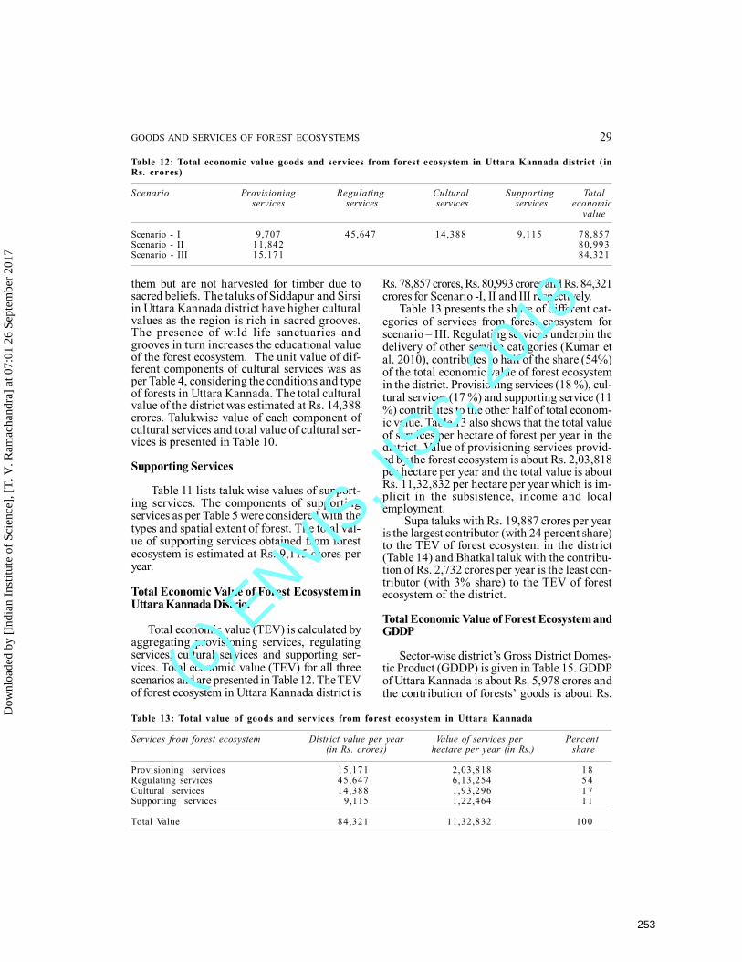
GOODS AND SERVICES OF FOREST ECOSYSTEMS 29
them but are not harvested for timber due tosacred beliefs. The taluks of Siddapur and Sirsiin Uttara Kannada district have higher culturalvalues as the region is rich in sacred grooves.The presence of wild life sanctuaries andgrooves in turn increases the educational valueof the forest ecosystem. The unit value of dif-ferent components of cultural services was asper Table 4, considering the conditions and typeof forests in Uttara Kannada. The total culturalvalue of the district was estimated at Rs. 14,388crores. Talukwise value of each component ofcultural services and total value of cultural ser-vices is presented in Table 10.
Supporting Services
Table 11 lists taluk wise values of support-ing services. The components of supportingservices as per Table 5 were considered with thetypes and spatial extent of forest. The total val-ue of supporting services obtained from forestecosystem is estimated at Rs. 9,115 crores peryear.
Total Economic Value of Forest Ecosystem inUttara Kannada District
Total economic value (TEV) is calculated byaggregating provisioning services, regulatingservices, cultural services and supporting ser-vices. Total economic value (TEV) for all threescenarios and are presented in Table 12. The TEVof forest ecosystem in Uttara Kannada district is
Rs. 78,857 crores, Rs. 80,993 crores and Rs. 84,321crores for Scenario -I, II and III respectively.
Table 13 presents the share of different cat-egories of services from forest ecosystem forscenario – III. Regulating services underpin thedelivery of other service categories (Kumar etal. 2010), contributes to half of the share (54%)of the total economic value of forest ecosystemin the district. Provisioning services (18 %), cul-tural services (17 %) and supporting service (11%) contributes to the other half of total econom-ic value. Table 13 also shows that the total valueof services per hectare of forest per year in thedistrict. Value of provisioning services provid-ed by the forest ecosystem is about Rs. 2,03,818per hectare per year and the total value is aboutRs. 11,32,832 per hectare per year which is im-plicit in the subsistence, income and localemployment.
Supa taluks with Rs. 19,887 crores per yearis the largest contributor (with 24 percent share)to the TEV of forest ecosystem in the district(Table 14) and Bhatkal taluk with the contribu-tion of Rs. 2,732 crores per year is the least con-tributor (with 3% share) to the TEV of forestecosystem of the district.
Total Economic Value of Forest Ecosystem andGDDP
Sector-wise district’s Gross District Domes-tic Product (GDDP) is given in Table 15. GDDPof Uttara Kannada is about Rs. 5,978 crores andthe contribution of forests’ goods is about Rs.
Table 13: Total value of goods and services from forest ecosystem in Uttara Kannada
Services from forest ecosystem District value per year Value of services per Percent(in Rs. crores) hectare per year (in Rs.) share
Provisioning services 15,171 2,03,818 1 8Regulating services 45,647 6,13,254 5 4Cultural services 14,388 1,93,296 1 7Supporting services 9,115 1,22,464 1 1
Total Value 84,321 11,32,832 100
Table 12: Total economic value goods and services from forest ecosystem in Uttara Kannada district ( inRs. crores)
Scenario Provisioning Regulating Cultural Supporting Totalservices services services services economic
value
Scenario - I 9,707 45,647 14,388 9,115 78,857Scenario - II 11,842 80,993Scenario - III 15,171 84,321
Dow
nloa
ded
by [
Indi
an I
nstit
ute
of S
cien
ce],
[T
. V. R
amac
hand
ra]
at 0
7:01
26
Sept
embe
r 20
17
253
(c) E
NVIS, I
ISc,
2018
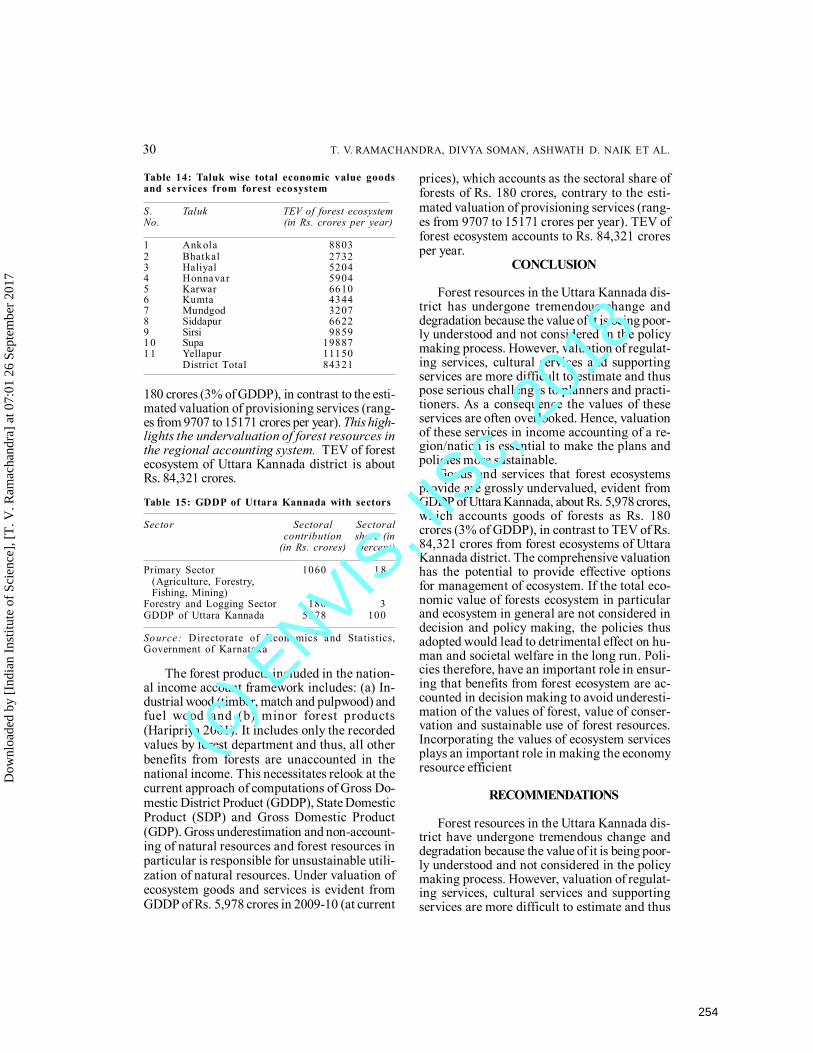
30 T. V. RAMACHANDRA, DIVYA SOMAN, ASHWATH D. NAIK ET AL.
180 crores (3% of GDDP), in contrast to the esti-mated valuation of provisioning services (rang-es from 9707 to 15171 crores per year). This high-lights the undervaluation of forest resources inthe regional accounting system. TEV of forestecosystem of Uttara Kannada district is aboutRs. 84,321 crores.
The forest products included in the nation-al income account framework includes: (a) In-dustrial wood (timber, match and pulpwood) andfuel wood and (b) minor forest products(Haripriya 2001). It includes only the recordedvalues by forest department and thus, all otherbenefits from forests are unaccounted in thenational income. This necessitates relook at thecurrent approach of computations of Gross Do-mestic District Product (GDDP), State DomesticProduct (SDP) and Gross Domestic Product(GDP). Gross underestimation and non-account-ing of natural resources and forest resources inparticular is responsible for unsustainable utili-zation of natural resources. Under valuation ofecosystem goods and services is evident fromGDDP of Rs. 5,978 crores in 2009-10 (at current
prices), which accounts as the sectoral share offorests of Rs. 180 crores, contrary to the esti-mated valuation of provisioning services (rang-es from 9707 to 15171 crores per year). TEV offorest ecosystem accounts to Rs. 84,321 croresper year.
CONCLUSION
Forest resources in the Uttara Kannada dis-trict has undergone tremendous change anddegradation because the value of it is being poor-ly understood and not considered in the policymaking process. However, valuation of regulat-ing services, cultural services and supportingservices are more difficult to estimate and thuspose serious challenges to planners and practi-tioners. As a consequence the values of theseservices are often overlooked. Hence, valuationof these services in income accounting of a re-gion/nation is essential to make the plans andpolicies more sustainable.
Goods and services that forest ecosystemsprovide are grossly undervalued, evident fromGDDP of Uttara Kannada, about Rs. 5,978 crores,which accounts goods of forests as Rs. 180crores (3% of GDDP), in contrast to TEV of Rs.84,321 crores from forest ecosystems of UttaraKannada district. The comprehensive valuationhas the potential to provide effective optionsfor management of ecosystem. If the total eco-nomic value of forests ecosystem in particularand ecosystem in general are not considered indecision and policy making, the policies thusadopted would lead to detrimental effect on hu-man and societal welfare in the long run. Poli-cies therefore, have an important role in ensur-ing that benefits from forest ecosystem are ac-counted in decision making to avoid underesti-mation of the values of forest, value of conser-vation and sustainable use of forest resources.Incorporating the values of ecosystem servicesplays an important role in making the economyresource efficient
RECOMMENDATIONS
Forest resources in the Uttara Kannada dis-trict have undergone tremendous change anddegradation because the value of it is being poor-ly understood and not considered in the policymaking process. However, valuation of regulat-ing services, cultural services and supportingservices are more difficult to estimate and thus
Table 15: GDDP of Uttara Kannada with sectors
Sector Sectoral Sectoralcontribution share (in
(in Rs. crores) percent)
Primary Sector 1060 1 8 (Agriculture, Forestry, Fishing, Mining)Forestry and Logging Sector 180 3GDDP of Uttara Kannada 5978 100
Source: Directorate of Economics and Statistics,Government of Karnataka
Table 14: Taluk wise total economic value goodsand services from forest ecosystem
S. Taluk TEV of forest ecosystemNo. (in Rs. crores per year)
1 Ankola 88032 Bhatkal 27323 Haliyal 52044 Honnavar 59045 Karwar 66106 Kumta 43447 Mundgod 32078 Siddapur 66229 Sirsi 98591 0 Supa 198871 1 Yellapur 11150
District Total 84321
Dow
nloa
ded
by [
Indi
an I
nstit
ute
of S
cien
ce],
[T
. V. R
amac
hand
ra]
at 0
7:01
26
Sept
embe
r 20
17
254
(c) E
NVIS, I
ISc,
2018
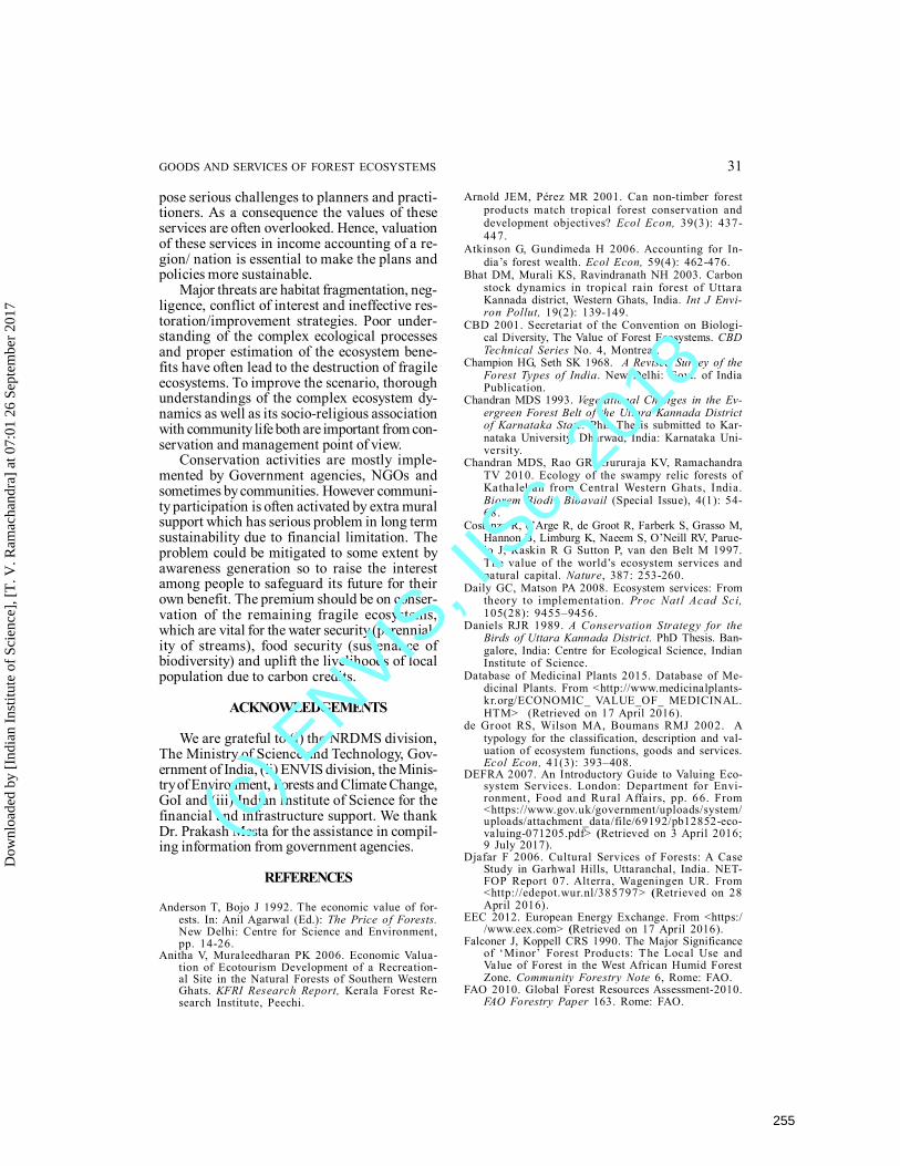
GOODS AND SERVICES OF FOREST ECOSYSTEMS 31
pose serious challenges to planners and practi-tioners. As a consequence the values of theseservices are often overlooked. Hence, valuationof these services in income accounting of a re-gion/ nation is essential to make the plans andpolicies more sustainable.
Major threats are habitat fragmentation, neg-ligence, conflict of interest and ineffective res-toration/improvement strategies. Poor under-standing of the complex ecological processesand proper estimation of the ecosystem bene-fits have often lead to the destruction of fragileecosystems. To improve the scenario, thoroughunderstandings of the complex ecosystem dy-namics as well as its socio-religious associationwith community life both are important from con-servation and management point of view.
Conservation activities are mostly imple-mented by Government agencies, NGOs andsometimes by communities. However communi-ty participation is often activated by extra muralsupport which has serious problem in long termsustainability due to financial limitation. Theproblem could be mitigated to some extent byawareness generation so to raise the interestamong people to safeguard its future for theirown benefit. The premium should be on conser-vation of the remaining fragile ecosystems,which are vital for the water security (perennial-ity of streams), food security (sustenance ofbiodiversity) and uplift the livelihoods of localpopulation due to carbon credits.
ACKNOWLEDGEMENTS
We are grateful to (i) the NRDMS division,The Ministry of Science and Technology, Gov-ernment of India, (ii) ENVIS division, the Minis-try of Environment, Forests and Climate Change,GoI and (iii) Indian Institute of Science for thefinancial and infrastructure support. We thankDr. Prakash Mesta for the assistance in compil-ing information from government agencies.
REFERENCES
Anderson T, Bojo J 1992. The economic value of for-ests. In: Anil Agarwal (Ed.): The Price of Forests.New Delhi: Centre for Science and Environment,pp. 14-26.
Anitha V, Muraleedharan PK 2006. Economic Valua-tion of Ecotourism Development of a Recreation-al Site in the Natural Forests of Southern WesternGhats. KFRI Research Report, Kerala Forest Re-search Institute, Peechi.
Arnold JEM, Pérez MR 2001. Can non-timber forestproducts match tropical forest conservation anddevelopment objectives? Ecol Econ, 39(3): 437-447.
Atkinson G, Gundimeda H 2006. Accounting for In-dia’s forest wealth. Ecol Econ, 59(4): 462-476.
Bhat DM, Murali KS, Ravindranath NH 2003. Carbonstock dynamics in tropical rain forest of UttaraKannada district, Western Ghats, India. Int J Envi-ron Pollut, 19(2): 139-149.
CBD 2001. Secretariat of the Convention on Biologi-cal Diversity, The Value of Forest Ecosystems. CBDTechnical Series No. 4, Montreal.
Champion HG, Seth SK 1968. A Revised Survey of theForest Types of India. New Delhi: Govt. of IndiaPublication.
Chandran MDS 1993. Vegetational Changes in the Ev-ergreen Forest Belt of the Uttara Kannada Districtof Karnataka State. PhD Thesis submitted to Kar-nataka University. Dharwad, India: Karnataka Uni-versity.
Chandran MDS, Rao GR, Gururaja KV, RamachandraTV 2010. Ecology of the swampy relic forests ofKathalekan from Central Western Ghats, India.Biorem Biodiv Bioavail (Special Issue), 4(1): 54-68.
Costanza R, d’Arge R, de Groot R, Farberk S, Grasso M,Hannon B, Limburg K, Naeem S, O’Neill RV, Parue-lo J, Raskin R G Sutton P, van den Belt M 1997.The value of the world’s ecosystem services andnatural capital. Nature, 387: 253-260.
Daily GC, Matson PA 2008. Ecosystem services: Fromtheory to implementation. Proc Natl Acad Sci,105(28): 9455–9456.
Daniels RJR 1989. A Conservation Strategy for theBirds of Uttara Kannada District. PhD Thesis. Ban-galore, India: Centre for Ecological Science, IndianInstitute of Science.
Database of Medicinal Plants 2015. Database of Me-dicinal Plants. From <http://www.medicinalplants-kr.org/ECONOMIC_ VALUE_OF_ MEDICINAL.HTM> (Retrieved on 17 April 2016).
de Groot RS, Wilson MA, Boumans RMJ 2002. Atypology for the classification, description and val-uation of ecosystem functions, goods and services.Ecol Econ, 41(3): 393–408.
DEFRA 2007. An Introductory Guide to Valuing Eco-system Services. London: Department for Envi-ronment, Food and Rural Affairs, pp. 66. From<https://www.gov.uk/government/uploads/system/uploads/attachment_data/file/69192/pb12852-eco-valuing-071205.pdf> (Retrieved on 3 April 2016;9 July 2017).
Djafar F 2006. Cultural Services of Forests: A CaseStudy in Garhwal Hills, Uttaranchal, India. NET-FOP Report 07. Alterra, Wageningen UR. From<http://edepot.wur.nl/385797> (Retrieved on 28April 2016).
EEC 2012. European Energy Exchange. From <https://www.eex.com> (Retrieved on 17 April 2016).
Falconer J, Koppell CRS 1990. The Major Significanceof ‘Minor’ Forest Products: The Local Use andValue of Forest in the West African Humid ForestZone. Community Forestry Note 6, Rome: FAO.
FAO 2010. Global Forest Resources Assessment-2010.FAO Forestry Paper 163. Rome: FAO.
Dow
nloa
ded
by [
Indi
an I
nstit
ute
of S
cien
ce],
[T
. V. R
amac
hand
ra]
at 0
7:01
26
Sept
embe
r 20
17
255
(c) E
NVIS, I
ISc,
2018
32 T. V. RAMACHANDRA, DIVYA SOMAN, ASHWATH D. NAIK ET AL.
Gera M, Yadav AKR, Bisht NS, Mohan G 2008. Valua-tion of recreational benefits from the valley offlowers National Park. Indian For, 134(1): 26-35.
Gonzalez P, Hassan R, Lakyda P, McCallum I, NilssonS, Pulhin J, Rosenburg B, Scholes B 2005. Forestand woodland systems. In: R Hassan, R Scholes, NAsh (Eds.): Ecosystems and Human Wellbeing: Vol-ume 1: Current State and Trends. Washington: Is-land Press, pp 68-77.
Gunderson LH, Cosens B, Garmestani AS 2016. Adaptivegovernance of riverine and wetland ecosystem goodsand services. Journal of Environmental Management,183(2): 353-360. doi.org/10.1016/j.jenvman. 2016.05.024.
Haripriya GS 2001. Integrated environmental and eco-nomic accounting: An application to the forestresources in India. Environ Resour Econ , 19(1):73-95.
Haripriya GS 2002. Biomass carbon of truncated diam-eter classes in Indian forests. Forest Ecol Manage,168(1-3): 1-13.
Harsha VH, Shripathi V, Hegde GR 2005. Ethno veter-inary practices in Uttara Kannada district of Kar-nataka. Indian J Tradit Know, 4(30): 253-258.
Hebbar SS, Hegde G, Hegde GR 2010. Less known wildedible fruits and seeds of Uttara Kannada district.Indian For, 136(9): 1218-1222.
Hegde HV, Hegde GR, Kholkute SD 2007. Herbal carefor reproductive health: Ethnomedicobotany fromUttara Kannada district, Karnataka, India. Com-plement Ther Clin Pract, 13(1): 38-45.
Kamath SU 1985. Uttara Kannada District. Karnata-ka State Gazetteer. Bangalore: Government of Kar-nataka.
KFD 2015. Karwar Division, Karnataka Forest De-partment. From <http://www.aranya.gov.in/Static%20Pages/Karwar.aspx> (Retrieved on 12 January2015, 18 June 2017; 9 July 2017).
KPCL 2016. Karnataka Power Corporation Limited.From <http://www.karnatakapower.com > (Retrievedon 17 April 2016).
Kramer RA, Sharma N, Munasinghe M 1995. ValuingTropical Forests: Methodology and Case Study ofMadagascar. World Bank Environment Paper No.13, Washington D.C.
Kumar P, Verma M, Wood MD, Negandhi D 2010.Guidance Manual for the Valuation of RegulatingServices. UNEP, Nairobi, 2010.
Lal M, Singh R 2000. Carbon sequestration potentialof Indian forests. Environ Monit Assess, 60(3): 315-327.
Mace GM 2005. Biodiversity: An index of intactness.Nature, 434(7029): 32-33.
Manoharan TR 1996. Economics of Protected Areas:A Case Study of Periyar Tiger Reserve. PhD Thesis.Dehra Dun: Forest Research Institute.
Maudgal S, Kakkar M 1992. Evaluation of forests forimpact assessment of development project. In: AAgarwal (Ed.): The Price of Forests. New Delhi:CSE, pp. 53-60.
MEA (Millennium Ecosystem Assessment) 2003. Eco-systems and Human Well-being: A Framework forAssessment. Washington, DC: Island Press.
Mohandas TV, Remadevi OK 2011. A study on touristvisitations in protected areas of central WesternGhats in Karnataka. Indian For, 137(4): 403-410.
Murthy IK, Bhat PR, Ravindranath NH, Sukumar R,2005. Financial valuation of non-timber forest prod-uct flows in Uttara Kannada district, Western Ghats,Karnataka. Curr Sci India, 88(10): 1573-1579.
Myers N 1984. The Primary Source: Tropical Forestsand Our Future. New York: W. W. Norton.
NABARD (National Bank for Agricultural and RuralDevelopment) 2015. From <http://www.nabard.org/modelbankprojects> (Retrieved on 12 January2015, 18 June 2017).
Nasi R, Wunder S, Campos AJJ 2002. Forest EcosystemServices: Can They Pay Our Way Out of Deforesta-tion? Bogor, Indonesia: CIFOR for the Global En-vironmental Facility (GEF).
Newcome J, Provins A, Johns H, Ozdemiroglu E, GhazoulJ, Burgess D, Turner K 2005. The Economic, So-cial and Ecological Value of Ecosystem Services: ALiterature Review. London: Economics for the En-vironment Consultancy.
NPCIL (Nuclear Power Corporation of India Limited)2016. From <http://www.npcil.nic.in/main/ProjectOperationDisplay.aspx?ReactorID=76&Page> (Re-trieved on 21 February 2016).
Panchamukhi PR, Trivedi P, Debi S, Kulkarni AK, Shar-ma P 2008. Natural Resource Accounting In Kar-nataka: A Study on Land and Forestry Sector (Ex-cluding Mining). Centre for Multi-Disciplinary De-velopment Research, Dharwad, p. 242. From<http://docplayer.net/45191657-Natural-resource-accounting-in-karnataka-a-study-of-the-land-for-estry-sector-excluding-mining.html> (Retrieved on28 September 2016; 9 July 2017).
Pearce DW, Moran D, Biller D 2002. Handbook ofBiodiversity Valuation: A Guide for Policy Makers.Paris and Washington, D.C.: OECD, p. 40. From< h t t p : / / p o r t a l s . w i . w u r . n l / f i l e s / d o c s / F i l e /nfp%20for%20all/FinancingMech/OECD Hand-book on Biodiversity Valuation.pdf> (Retrieved on28 September 2016).
Peters CM, Gentry AH, Mendelsohn RO 1989. Valua-tion of an Amazonian rainforest. Nature, 339: 655-656.
Pittini M 2011. Monetary Valuation for Ecosystem Ac-counting. Issue Paper Prepared for the UN/WorldBank/EEA Expert Meeting on Ecosystem Accounts,London., p. 30. From <https://unstats.un.org/unsd/envaccounting/seeaLES/egm/Issue10_UK.pdf> (Re-trieved on 28 September 2016; 9 July 2017).
Prasad SN, Hedge M, Hedge MS 1987b. Fuel Consump-tion and Conservation Method in Urban Centres ofUttara Kannada. CES Technical Report 25. CES, IISc,Bangalore.
Prasad SN, Hegde HG, Bhat DM, Hegde M 1987a. Esti-mates of Standing Biomass and Productivity of Trop-ical Moist Forest of Uttara Kannada District, Karna-taka, India. CES Technical Report No. 19, CES, IISc,Bangalore.
PSP 2016. Parrys Sugar Factory. From <http://www.parrysugar.in/html/locations-Haliyal > (Retrievedon 28 September 2016; 9 July 2017).
Raghunath HM 2006. Hydrology: Principles, Analysisand Design. New Delhi: Wiley Eastern Limited.
Ramachandra TV, Nagarathna AV 2001. Energetics inpaddy cultivation in Uttara Kannada District. EnergConvers and Manage, 42(2): 132-155.
Dow
nloa
ded
by [
Indi
an I
nstit
ute
of S
cien
ce],
[T
. V. R
amac
hand
ra]
at 0
7:01
26
Sept
embe
r 20
17
256
(c) E
NVIS, I
ISc,
2018
GOODS AND SERVICES OF FOREST ECOSYSTEMS 33
Ramachandra TV 1998. Energy utilisation in rural indus-tries in Karnataka. Int J Ambient Energy, 19(2): 75-92.
Ramachandra TV, Subramanian DK, Joshi NV 1999.Hydroelectric resource assessment in Uttara Kanna-da District, Karnataka State, India. J Clean Prod,7(3): 195-211.
Ramachandra TV, Joshi NV, Subramanian DK 2000.Present and prospective role of bioenergy in re-gional energy system. Renew Sust Energ Rev, 4(4):375-430.
Ramachandra TV, Kamakshi G, Shruthi BV 2004. Biore-source status in Karnataka. Renew Sust Energ Rev,8(1): 1-47.
Ramachandra TV, Ganapathy S 2007. Vegetation Anal-ysis in Uttara Kannada District Using GIS and Re-mote Sensing Techniques. ENVIS Technical ReportNo . 24, Environmental Information System, CES,IISc, Bangalore.
Ramachandra TV, Chandran MDS, Gururaja KV, Sree-kantha 2007. Cumulative Environmental ImpactAssessment. New York: Nova Science Publishers.
Ramachandra TV, Alakananda B, Ali Rani, Khan MA2011. Ecological and socio-economic assessmentof Varthur wetland, Bengaluru, India. J Environ SciEng, 53(1): 101-108.
Ramachandra TV, Chandran MDS, Joshi NV, Balachan-dran C 2012. Beekeeping: Sustainable LivelihoodOption in Uttara Kannada, Central Western Ghats.ENVIS Technical Report No . 19, EnvironmentalInformation System, CES, IISc, Bangalore.
Ramachandra TV, Subramanian DK, Joshi NV, GunagaSV, Harikanta RB 2000. Domestic energy consump-tion patterns in Uttara Kannada district, Karnata-ka state, India. Energ Convers Manage, 41(8): 775-831.
Ramachandra TV, Chandran MDS, Joshi NV, KarthickB, Mukri VD 2015. Ecohydrology of Lotic Systemsin Uttara Kannada, Central Western Ghats, India.Springer: Environmental Management of River Ba-sin Ecosystems, Springer Earth System Sciences.
Ramachandra TV, Bharath Setturu, Rajan KS, Chan-dran MDS 2016a. Stimulus of DevelopmentalProjects to Landscape Dynamics in Uttara Kanna-da, Central Western Ghats. The Egyptian Journalof Remote Sensing and Space Sciences. From <http://dx.doi.org/10.1016/j.ejrs.2016.09.001>, pp.1-19.
Ramachandra, TV, Vinay S, Aithal BH 2016b. Envi-ronmental flow assessment in a lotic ecosystem ofCentral Western Ghats, India. Hydrol Curr Res, 7:1-14.
Ramana P, Patil SK 2008. Marketing of value addedproducts from Artocarpus species in Uttara Kanna-da district of Karnataka. My Forest, 44(1): 49-53.
Rao GR, Mesta D, Chandran MDS, Ramachandra TV2008. Wetland flora of Uttara Kannada. In: TVRamachandra (Ed.): Environmental Education forEcosystem Conservation. New Delhi: Capital Pub-lishing Company, pp 140-152.
Ray R, Chandran MDS, Ramachandra TV 2011. SacredGroves in Siddapur Taluk, Uttara Kannada, Karna-taka: Threats and Management Aspects. ENVIS Tech-nical Report 38, Environmental Information Sys-tem, CES, IISc, Bangalore.
Ray R, Ramachandra TV 2011. Small sacred groves inlocal landscape: Are they really worth for conser-vation? Curr Sci India, 98(9): 1178-1180.
Ray R, Chandran MDS, Ramachandra TV 2015. Hy-drological importance of sacred forest fragmentsin Central Western Ghats of India. Trop Ecol, 56:87-99.
Schaafsma M, Morse-Jones S, Posen P, Swetnam R.D,Balmford A, Bateman IJ, Burgess ND, ChamshamaSAO., Fisher B, Freeman T, Geofrey V, Green RE,Hepelwa AS, Turner RK 2014. The importance oflocal forest benefits: Economic valuation of Non-Timber Forest Products in the Eastern Arc Moun-tains in Tanzania. Global Environmental Change,24(2014): 295-305.
SCIL 2015. Solaris Chemtech Industries Limited, Bi-naga, Karwar. From <http://www. solarischemtech.com/infra-falt.asp?links=falt> (Retrieved on 17 June2015).
Seema D, Ramachandra TV 2010. Carbon Sequestra-tion Potential of Ecosystems in Uttara KannadaDistrict, Western Ghats of Karnataka, India, In: TVRamachandra (Ed.): Proceedings of Lake 2010: Con-ference on Wetlands, Biodiversity and ClimateChange, 22-24 Dec. 2010, Bangalore, pp. 162-178.From <http://wgbis.ces.iisc.ernet.in/energy/lake2010/Theme%201/seema_day.pdf>.
Simpson RD, Sedjo RA, Reid JW 1996. Valuing biodi-versity for use in pharmaceutical research. The J ofPolit Econ, 104(1): 163-185.
TEEB 2010. The Economics of Ecosystems and Biodi-versity Ecological and Economic Foundations. Push-pam Kumar (Ed.). London and Washington: Earth-scan, pp 31-224. From <http://www.teebweb.org/our-publications/teeb-study-reports/ecological-and-economic-foundations>. (Retrieved on 21 Febru-ary 2016)
Tewari DD, Campbell JY 1996. Increased Develop-ment of Non-Timber Forest Products in India: SomeIssues and Concern. Unasylva, 47(187): 26-31.From <http://www.fao.org/docrep/w2149e/w2149e06.htm#increased development of non timberforest products in India: some issues and co> (Re-trieved on 17 January 2015).
Verma M, Joshi S, Godbole G, Singh A 2007. Valuationof Ecosystem Services and Forest Governance: AScoping Study from Uttarakhand, Leadership inEnvironment and Development (LEAD-India),New Delhi. Pp 125. From <http://www. leadindia.org> (Retrieved on 21 February 2016)
Villegas-Palacio C, Berrouet L, Connie L, Ruiz A, UpeguiA 2016. Lessons from the integrated valuation ofecosystem services in a developing country: Threecase studies on ecological, socio-cultural and economicvaluation. Ecosystem Services, 22(2016): 297-308.http://dx.doi.org/10.1016/j.ecoser.2016. 10.017
WCPM 2016. West Cosast Paper Mill, Dandeli. From<http:// westcoastpaper.com/index.php?q=node/23> (Retrieved on 22 October 2016).
Paper received for publication on February 2017Paper accepted for publication on July 2017
Dow
nloa
ded
by [
Indi
an I
nstit
ute
of S
cien
ce],
[T
. V. R
amac
hand
ra]
at 0
7:01
26
Sept
embe
r 20
17
257
(c) E
NVIS, I
ISc,
2018
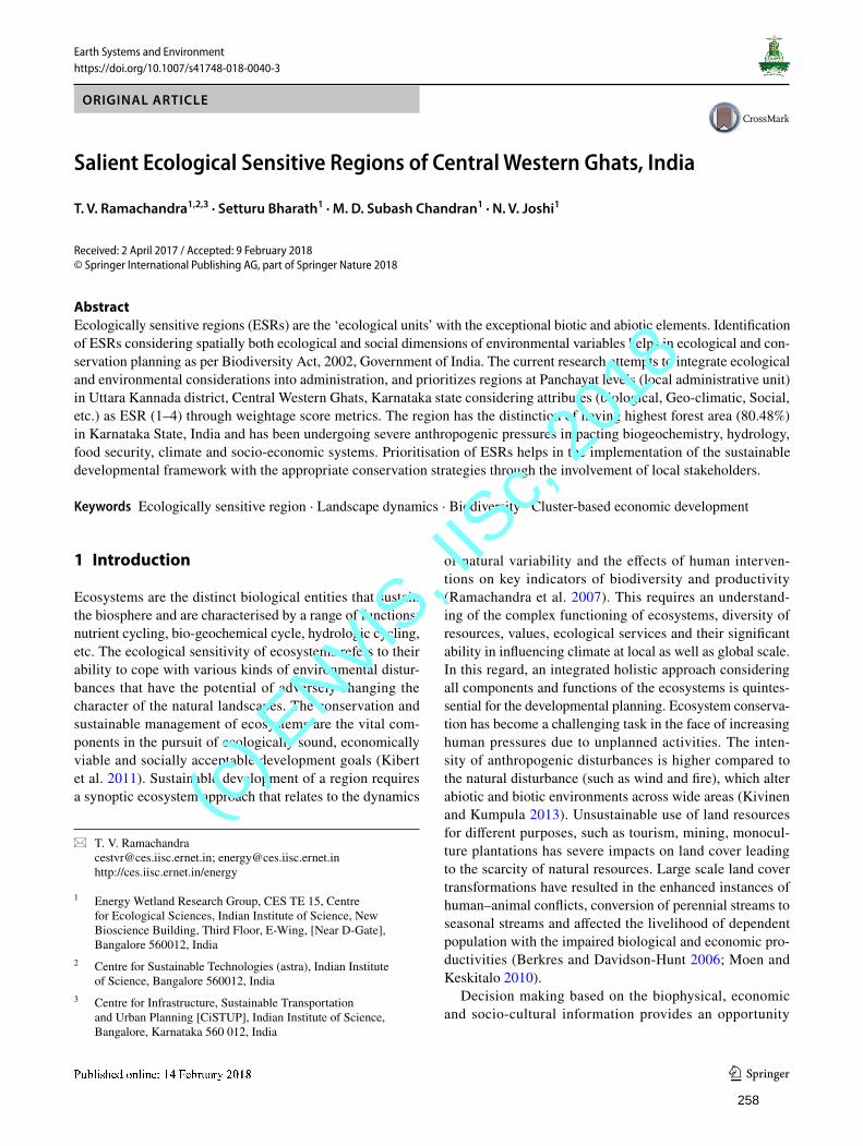
Vol.:(0123456789)1 3
Earth Systems and Environment https://doi.org/10.1007/s41748-018-0040-3
ORIGINAL ARTICLE
Salient Ecological Sensitive Regions of Central Western Ghats, India
T. V. Ramachandra1,2,3 · Setturu Bharath1 · M. D. Subash Chandran1 · N. V. Joshi1
Received: 2 April 2017 / Accepted: 9 February 2018 © Springer International Publishing AG, part of Springer Nature 2018
AbstractEcologically sensitive regions (ESRs) are the ‘ecological units’ with the exceptional biotic and abiotic elements. Identification of ESRs considering spatially both ecological and social dimensions of environmental variables helps in ecological and con-servation planning as per Biodiversity Act, 2002, Government of India. The current research attempts to integrate ecological and environmental considerations into administration, and prioritizes regions at Panchayat levels (local administrative unit) in Uttara Kannada district, Central Western Ghats, Karnataka state considering attributes (biological, Geo-climatic, Social, etc.) as ESR (1–4) through weightage score metrics. The region has the distinction of having highest forest area (80.48%) in Karnataka State, India and has been undergoing severe anthropogenic pressures impacting biogeochemistry, hydrology, food security, climate and socio-economic systems. Prioritisation of ESRs helps in the implementation of the sustainable developmental framework with the appropriate conservation strategies through the involvement of local stakeholders.
Keywords Ecologically sensitive region · Landscape dynamics · Biodiversity · Cluster-based economic development
1 Introduction
Ecosystems are the distinct biological entities that sustain the biosphere and are characterised by a range of functions: nutrient cycling, bio-geochemical cycle, hydrologic cycling, etc. The ecological sensitivity of ecosystems refers to their ability to cope with various kinds of environmental distur-bances that have the potential of adversely changing the character of the natural landscapes. The conservation and sustainable management of ecosystems are the vital com-ponents in the pursuit of ecologically sound, economically viable and socially acceptable development goals (Kibert et al. 2011). Sustainable development of a region requires a synoptic ecosystem approach that relates to the dynamics
of natural variability and the effects of human interven-tions on key indicators of biodiversity and productivity (Ramachandra et al. 2007). This requires an understand-ing of the complex functioning of ecosystems, diversity of resources, values, ecological services and their significant ability in influencing climate at local as well as global scale. In this regard, an integrated holistic approach considering all components and functions of the ecosystems is quintes-sential for the developmental planning. Ecosystem conserva-tion has become a challenging task in the face of increasing human pressures due to unplanned activities. The inten-sity of anthropogenic disturbances is higher compared to the natural disturbance (such as wind and fire), which alter abiotic and biotic environments across wide areas (Kivinen and Kumpula 2013). Unsustainable use of land resources for different purposes, such as tourism, mining, monocul-ture plantations has severe impacts on land cover leading to the scarcity of natural resources. Large scale land cover transformations have resulted in the enhanced instances of human–animal conflicts, conversion of perennial streams to seasonal streams and affected the livelihood of dependent population with the impaired biological and economic pro-ductivities (Berkres and Davidson-Hunt 2006; Moen and Keskitalo 2010).
Decision making based on the biophysical, economic and socio-cultural information provides an opportunity
* T. V. Ramachandra [email protected]; [email protected] http://ces.iisc.ernet.in/energy
1 Energy Wetland Research Group, CES TE 15, Centre for Ecological Sciences, Indian Institute of Science, New Bioscience Building, Third Floor, E-Wing, [Near D-Gate], Bangalore 560012, India
2 Centre for Sustainable Technologies (astra), Indian Institute of Science, Bangalore 560012, India
3 Centre for Infrastructure, Sustainable Transportation and Urban Planning [CiSTUP], Indian Institute of Science, Bangalore, Karnataka 560 012, India
258
(c) E
NVIS, I
ISc,
2018
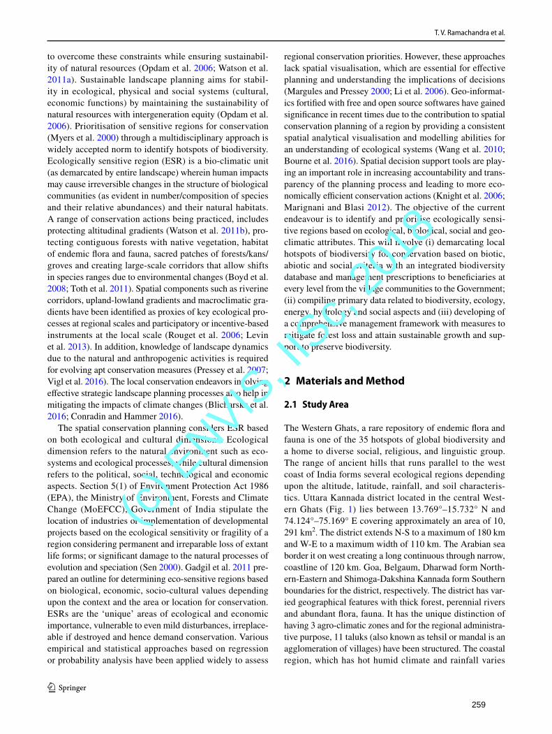
T. V. Ramachandra et al.
1 3
to overcome these constraints while ensuring sustainabil-ity of natural resources (Opdam et al. 2006; Watson et al. 2011a). Sustainable landscape planning aims for stabil-ity in ecological, physical and social systems (cultural, economic functions) by maintaining the sustainability of natural resources with intergeneration equity (Opdam et al. 2006). Prioritisation of sensitive regions for conservation (Myers et al. 2000) through a multidisciplinary approach is widely accepted norm to identify hotspots of biodiversity. Ecologically sensitive region (ESR) is a bio-climatic unit (as demarcated by entire landscape) wherein human impacts may cause irreversible changes in the structure of biological communities (as evident in number/composition of species and their relative abundances) and their natural habitats. A range of conservation actions being practiced, includes protecting altitudinal gradients (Watson et al. 2011b), pro-tecting contiguous forests with native vegetation, habitat of endemic flora and fauna, sacred patches of forests/kans/groves and creating large-scale corridors that allow shifts in species ranges due to environmental changes (Boyd et al. 2008; Toth et al. 2011). Spatial components such as riverine corridors, upland-lowland gradients and macroclimatic gra-dients have been identified as proxies of key ecological pro-cesses at regional scales and participatory or incentive-based instruments at the local scale (Rouget et al. 2006; Levin et al. 2013). In addition, knowledge of landscape dynamics due to the natural and anthropogenic activities is required for evolving apt conservation measures (Pressey et al. 2007; Vigl et al. 2016). The local conservation endeavors involving effective strategic landscape planning processes also help in mitigating the impacts of climate changes (Blicharska et al. 2016; Conradin and Hammer 2016).
The spatial conservation planning considers ESR based on both ecological and cultural dimensions. Ecological dimension refers to the natural environment such as eco-systems and ecological processes, while cultural dimension refers to the political, social, technological and economic aspects. Section 5(1) of Environment Protection Act 1986 (EPA), the Ministry of Environment, Forests and Climate Change (MoEFCC), Government of India stipulate the location of industries or implementation of developmental projects based on the ecological sensitivity or fragility of a region considering permanent and irreparable loss of extant life forms; or significant damage to the natural processes of evolution and speciation (Sen 2000). Gadgil et al. 2011 pre-pared an outline for determining eco-sensitive regions based on biological, economic, socio-cultural values depending upon the context and the area or location for conservation. ESRs are the ‘unique’ areas of ecological and economic importance, vulnerable to even mild disturbances, irreplace-able if destroyed and hence demand conservation. Various empirical and statistical approaches based on regression or probability analysis have been applied widely to assess
regional conservation priorities. However, these approaches lack spatial visualisation, which are essential for effective planning and understanding the implications of decisions (Margules and Pressey 2000; Li et al. 2006). Geo-informat-ics fortified with free and open source softwares have gained significance in recent times due to the contribution to spatial conservation planning of a region by providing a consistent spatial analytical visualisation and modelling abilities for an understanding of ecological systems (Wang et al. 2010; Bourne et al. 2016). Spatial decision support tools are play-ing an important role in increasing accountability and trans-parency of the planning process and leading to more eco-nomically efficient conservation actions (Knight et al. 2006; Marignani and Blasi 2012). The objective of the current endeavour is to identify and prioritise ecologically sensi-tive regions based on ecological, biological, social and geo-climatic attributes. This will involve (i) demarcating local hotspots of biodiversity for conservation based on biotic, abiotic and social criteria with an integrated biodiversity database and management prescriptions to beneficiaries at every level from the village communities to the Government; (ii) compiling primary data related to biodiversity, ecology, energy, hydrology and social aspects and (iii) developing of a comprehensive management framework with measures to mitigate forest loss and attain sustainable growth and sup-port to preserve biodiversity.
2 Materials and Method
2.1 Study Area
The Western Ghats, a rare repository of endemic flora and fauna is one of the 35 hotspots of global biodiversity and a home to diverse social, religious, and linguistic group. The range of ancient hills that runs parallel to the west coast of India forms several ecological regions depending upon the altitude, latitude, rainfall, and soil characteris-tics. Uttara Kannada district located in the central West-ern Ghats (Fig. 1) lies between 13.769°–15.732° N and 74.124°–75.169° E covering approximately an area of 10, 291 km2. The district extends N-S to a maximum of 180 km and W-E to a maximum width of 110 km. The Arabian sea border it on west creating a long continuous through narrow, coastline of 120 km. Goa, Belgaum, Dharwad form North-ern-Eastern and Shimoga-Dakshina Kannada form Southern boundaries for the district, respectively. The district has var-ied geographical features with thick forest, perennial rivers and abundant flora, fauna. It has the unique distinction of having 3 agro-climatic zones and for the regional administra-tive purpose, 11 taluks (also known as tehsil or mandal is an agglomeration of villages) have been structured. The coastal region, which has hot humid climate and rainfall varies
259
(c) E
NVIS, I
ISc,
2018
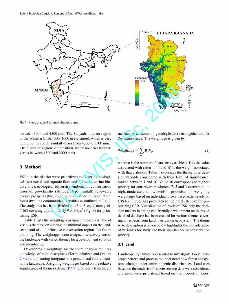
Salient Ecological Sensitive Regions of Central Western Ghats, India
1 3
between 3000 and 4500 mm. The Sahyadri interior region of the Western Ghats (500–1000 m elevation), which is very humid to the south (rainfall varies from 4000 to 5500 mm). The plains are regions of transition, which are drier (rainfall varies between 1500 and 2000 mm).
3 Method
ESRs in the district were prioritized considering biologi-cal (terrestrial and aquatic flora and fauna, estuarine bio-diversity), ecological (diversity, endemism, conservation reserve), geo-climatic (altitude, slope, rainfall), renewable energy prospects (bio, solar, wind), and social (population, forest dwelling communities) variables as outlined in Fig. 2. The study area has been divided into 5′ × 5′ equal area grids (168) covering approximately 9 × 9 km2 (Fig. 3) for prior-itizing ESR.
Table 1 lists the weightages assigned to each variable of various themes considering the minimal impact on the land-scape and also to prioritise conservation regions for future planning. The weightages were assigned iteratively across the landscape with varied themes for a development solution and monitoring.
Developing a weightage metric score analysis requires knowledge of multi disciplines (Termorshuizen and Opdam 2009) and planning integrates the present and future needs in the landscape. Assigning weightages based on the relative significance of themes (Beinat 1997) provides a transparent
mechanism for combining multiple data sets together to infer the significance. The weightage is given by,
where n is the number of data sets (variables), Vi is the value associated with criterion i, and Wi is the weight associated with that criterion. Table 1 expresses the theme wise deci-sion variable considered with their level of significance, ranked between 1 and 10. Value 10 corresponds to highest priority for conservation whereas 7, 5 and 3 correspond to high, moderate and low levels of prioritisation. Assigning weightages based on individual proxy based extensively on GIS techniques has proved to be the most effective for pri-oritizing ESR. Visualisation of levels of ESR help the deci-sion makers in opting eco-friendly development measures. A detailed database has been created for various themes cover-ing all aspects from land to estuarine ecosystem. The theme wise description is given below highlights the consideration of variables for study and their significance in conservation priority.
3.1 Land
Landscape dynamics is essential to investigate forest land-scape pattern and process to understand how forest ecosys-tems change under anthropogenic disturbances. Land uses based on the analysis of remote sensing data were considered and grids were prioritised based on the proportion forest
(1)Weighatge =
n∑
i=1
WiVi,
Fig. 1 Study area and its agro-climatic zones
260
(c) E
NVIS, I
ISc,
2018
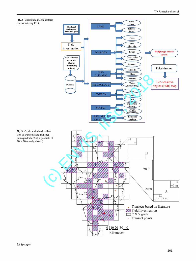
T. V. Ramachandra et al.
1 3
Fig. 2 Weightage metric criteria for prioritizing ESR
Fig. 3 Grids with the distribu-tion of transects and transect cum quadrats (2 of 5 quadrats of 20 × 20 m only shown)
261
(c) E
NVIS, I
ISc,
2018
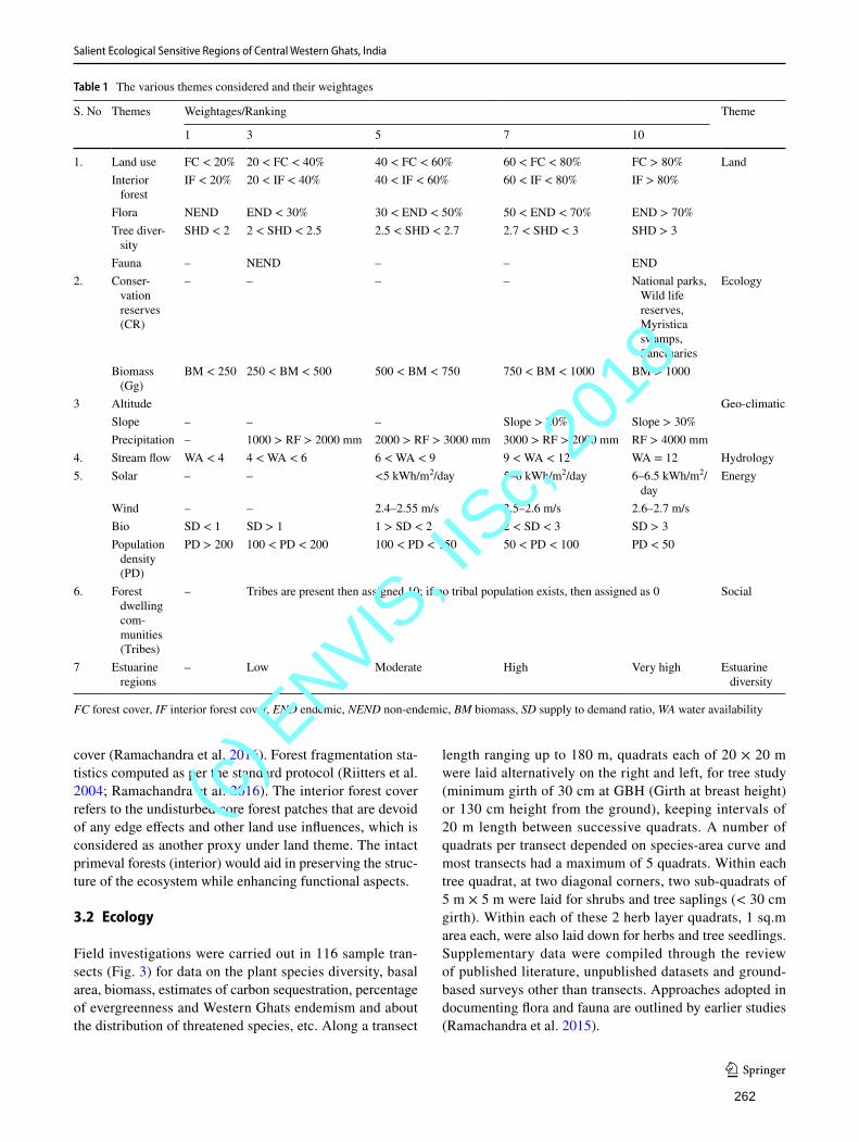
Salient Ecological Sensitive Regions of Central Western Ghats, India
1 3
cover (Ramachandra et al. 2016). Forest fragmentation sta-tistics computed as per the standard protocol (Riitters et al. 2004; Ramachandra et al. 2016). The interior forest cover refers to the undisturbed core forest patches that are devoid of any edge effects and other land use influences, which is considered as another proxy under land theme. The intact primeval forests (interior) would aid in preserving the struc-ture of the ecosystem while enhancing functional aspects.
3.2 Ecology
Field investigations were carried out in 116 sample tran-sects (Fig. 3) for data on the plant species diversity, basal area, biomass, estimates of carbon sequestration, percentage of evergreenness and Western Ghats endemism and about the distribution of threatened species, etc. Along a transect
length ranging up to 180 m, quadrats each of 20 × 20 m were laid alternatively on the right and left, for tree study (minimum girth of 30 cm at GBH (Girth at breast height) or 130 cm height from the ground), keeping intervals of 20 m length between successive quadrats. A number of quadrats per transect depended on species-area curve and most transects had a maximum of 5 quadrats. Within each tree quadrat, at two diagonal corners, two sub-quadrats of 5 m × 5 m were laid for shrubs and tree saplings (< 30 cm girth). Within each of these 2 herb layer quadrats, 1 sq.m area each, were also laid down for herbs and tree seedlings. Supplementary data were compiled through the review of published literature, unpublished datasets and ground-based surveys other than transects. Approaches adopted in documenting flora and fauna are outlined by earlier studies (Ramachandra et al. 2015).
Table 1 The various themes considered and their weightages
FC forest cover, IF interior forest cover, END endemic, NEND non-endemic, BM biomass, SD supply to demand ratio, WA water availability
S. No Themes Weightages/Ranking Theme
1 3 5 7 10
1. Land use FC < 20% 20 < FC < 40% 40 < FC < 60% 60 < FC < 80% FC > 80% LandInterior
forestIF < 20% 20 < IF < 40% 40 < IF < 60% 60 < IF < 80% IF > 80%
Flora NEND END < 30% 30 < END < 50% 50 < END < 70% END > 70%Tree diver-
sitySHD < 2 2 < SHD < 2.5 2.5 < SHD < 2.7 2.7 < SHD < 3 SHD > 3
Fauna – NEND – – END2. Conser-
vation reserves (CR)
– – – – National parks, Wild life reserves, Myristica swamps, Sanctuaries
Ecology
Biomass (Gg)
BM < 250 250 < BM < 500 500 < BM < 750 750 < BM < 1000 BM > 1000
3 Altitude Geo-climaticSlope – – – Slope > 20% Slope > 30%Precipitation – 1000 > RF > 2000 mm 2000 > RF > 3000 mm 3000 > RF > 2000 mm RF > 4000 mm
4. Stream flow WA < 4 4 < WA < 6 6 < WA < 9 9 < WA < 12 WA = 12 Hydrology5. Solar – – <5 kWh/m2/day 5–6 kWh/m2/day 6–6.5 kWh/m2/
dayEnergy
Wind – – 2.4–2.55 m/s 2.5–2.6 m/s 2.6–2.7 m/sBio SD < 1 SD > 1 1 > SD < 2 2 < SD < 3 SD > 3Population
density (PD)
PD > 200 100 < PD < 200 100 < PD < 150 50 < PD < 100 PD < 50
6. Forest dwelling com-munities (Tribes)
– Tribes are present then assigned 10; if no tribal population exists, then assigned as 0 Social
7 Estuarine regions
– Low Moderate High Very high Estuarine diversity
262
(c) E
NVIS, I
ISc,
2018
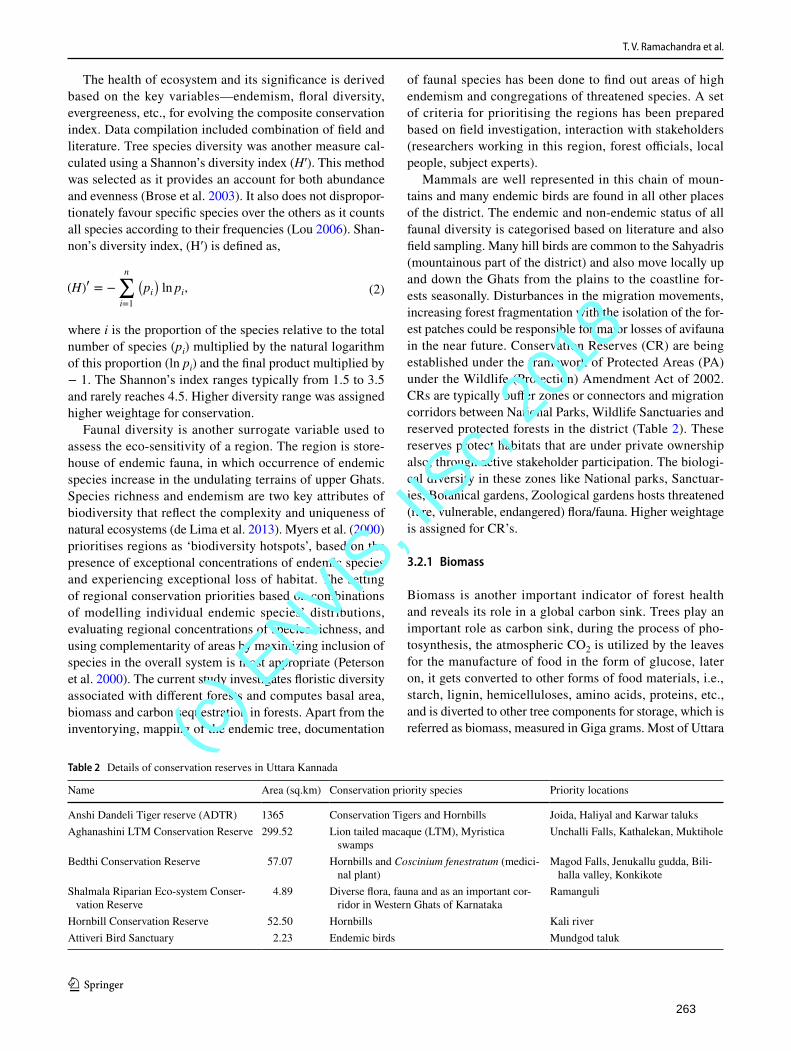
T. V. Ramachandra et al.
1 3
The health of ecosystem and its significance is derived based on the key variables—endemism, floral diversity, evergreeness, etc., for evolving the composite conservation index. Data compilation included combination of field and literature. Tree species diversity was another measure cal-culated using a Shannon’s diversity index (H′). This method was selected as it provides an account for both abundance and evenness (Brose et al. 2003). It also does not dispropor-tionately favour specific species over the others as it counts all species according to their frequencies (Lou 2006). Shan-non’s diversity index, (H′) is defined as,
where i is the proportion of the species relative to the total number of species (pi) multiplied by the natural logarithm of this proportion (ln pi) and the final product multiplied by − 1. The Shannon’s index ranges typically from 1.5 to 3.5 and rarely reaches 4.5. Higher diversity range was assigned higher weightage for conservation.
Faunal diversity is another surrogate variable used to assess the eco-sensitivity of a region. The region is store-house of endemic fauna, in which occurrence of endemic species increase in the undulating terrains of upper Ghats. Species richness and endemism are two key attributes of biodiversity that reflect the complexity and uniqueness of natural ecosystems (de Lima et al. 2013). Myers et al. (2000) prioritises regions as ‘biodiversity hotspots’, based on the presence of exceptional concentrations of endemic species and experiencing exceptional loss of habitat. The setting of regional conservation priorities based on combinations of modelling individual endemic species’ distributions, evaluating regional concentrations of species richness, and using complementarity of areas by maximizing inclusion of species in the overall system is most appropriate (Peterson et al. 2000). The current study investigates floristic diversity associated with different forests and computes basal area, biomass and carbon sequestration in forests. Apart from the inventorying, mapping of the endemic tree, documentation
(2)(H)� = −
n∑
i=1
(
pi)
ln pi,
of faunal species has been done to find out areas of high endemism and congregations of threatened species. A set of criteria for prioritising the regions has been prepared based on field investigation, interaction with stakeholders (researchers working in this region, forest officials, local people, subject experts).
Mammals are well represented in this chain of moun-tains and many endemic birds are found in all other places of the district. The endemic and non-endemic status of all faunal diversity is categorised based on literature and also field sampling. Many hill birds are common to the Sahyadris (mountainous part of the district) and also move locally up and down the Ghats from the plains to the coastline for-ests seasonally. Disturbances in the migration movements, increasing forest fragmentation with the isolation of the for-est patches could be responsible for major losses of avifauna in the near future. Conservation Reserves (CR) are being established under the framework of Protected Areas (PA) under the Wildlife (Protection) Amendment Act of 2002. CRs are typically buffer zones or connectors and migration corridors between National Parks, Wildlife Sanctuaries and reserved protected forests in the district (Table 2). These reserves protect habitats that are under private ownership also, through active stakeholder participation. The biologi-cal diversity in these zones like National parks, Sanctuar-ies, Botanical gardens, Zoological gardens hosts threatened (rare, vulnerable, endangered) flora/fauna. Higher weightage is assigned for CR’s.
3.2.1 Biomass
Biomass is another important indicator of forest health and reveals its role in a global carbon sink. Trees play an important role as carbon sink, during the process of pho-tosynthesis, the atmospheric CO2 is utilized by the leaves for the manufacture of food in the form of glucose, later on, it gets converted to other forms of food materials, i.e., starch, lignin, hemicelluloses, amino acids, proteins, etc., and is diverted to other tree components for storage, which is referred as biomass, measured in Giga grams. Most of Uttara
Table 2 Details of conservation reserves in Uttara Kannada
Name Area (sq.km) Conservation priority species Priority locations
Anshi Dandeli Tiger reserve (ADTR) 1365 Conservation Tigers and Hornbills Joida, Haliyal and Karwar taluksAghanashini LTM Conservation Reserve 299.52 Lion tailed macaque (LTM), Myristica
swampsUnchalli Falls, Kathalekan, Muktihole
Bedthi Conservation Reserve 57.07 Hornbills and Coscinium fenestratum (medici-nal plant)
Magod Falls, Jenukallu gudda, Bili-halla valley, Konkikote
Shalmala Riparian Eco-system Conser-vation Reserve
4.89 Diverse flora, fauna and as an important cor-ridor in Western Ghats of Karnataka
Ramanguli
Hornbill Conservation Reserve 52.50 Hornbills Kali riverAttiveri Bird Sanctuary 2.23 Endemic birds Mundgod taluk
263
(c) E
NVIS, I
ISc,
2018
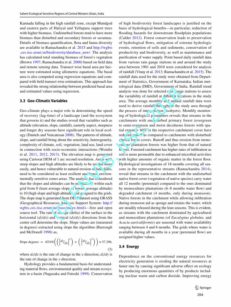
Salient Ecological Sensitive Regions of Central Western Ghats, India
1 3
Kannada falling in the high rainfall zone, except Mundgod and eastern parts of Haliyal and Yellapura support trees with higher biomass. Undisturbed forests tend to have more biomass than disturbed and secondary forests or savannas. Details of biomass quantification, flora and fauna diversity are available in Ramachandra et al. 2015 and http://wgbis .ces.iisc.ernet .in/biodi versi ty/datab ase_new/. The analysis has calculated total standing biomass of forest’s vegetation (Brown 1997; Ramachandra et al. 2000) based on field data and remote sensing data. Transect wise basal area per hec-tare were estimated using allometric equations. The basal area is also computed using regression equations and com-pared with field transect wise estimations. This approach has revealed the strong relationship between predicted basal area and estimated values using regression.
3.3 Geo‑Climatic Variables
Geo-climate plays a major role in determining the speed of recovery (lag-time) of a landscape (and the ecosystem that governs it) and the studies reveal that variables such as altitude (elevation, slope, rainfall), easterly aspect, steepness and longer dry seasons have significant role in local ecol-ogy (Daniels and Vencatesan 2008). The patterns of altitude, slope, and rainfall bring about the sensitivity, heterogeneity, complexity of climate, soil, vegetation, land use, land cover in connection with socio-economic interactions (Wondie et al. 2011, 2012, 2013). The elevation map is generated using Cartosat DEM of 1 arc second resolution. Areas with steep slopes and high altitudes are likely to be eroded more easily, and hence vulnerable to natural erosion or landslides, need to be considered as least resilient and hence environ-mentally sensitive zones areas. The analysis has considered that the slopes and altitudes can be normalized within each grid from 0 (least average slope or lowest average altitude) to 10 (high slope and high altitude) and assigned to the grids. The slope map is generated from DEM dataset using GRASS (Geographical Resources Analysis Support System- http://wgbis .ces.iisc.ernet .in/grass /index .html)—free and open source tool. The rate of change (delta) of the surface in the horizontal (dz/dx) and vertical (dz/dy) directions from the center cell determine the slope. Slope values are (measured in degrees) extracted using slope the algorithm (Burrough and McDonell 1998) as,
where dz/dx is the rate of change in the x-direction; dz/dy is the rate of change in the y-direction.
Hydrology provides a fundamental basis for understand-ing material flows, environmental quality and stream ecosys-tem in a basin (Nagasaka and Futoshi 1999). Conservation
(3)
Slope degrees = ATAN
((
[
dz∕dx
]2)
+
(
[
dz∕dy
]2))
× 57.296,
of high biodiversity forest landscapes is justified on the basis of hydrological benefits—in particular, reduction of flooding hazards for downstream floodplain populations (Calder 2012). Forest conservation leads to preservation of hydrological flows, mitigation of extreme hydrologic events, retention of soils and sediments, conservation of productivity and biodiversity, as well as maintenance and purification of water supply. Point based daily rainfall data from various rain gauge stations in and around the study area between 1901 and 2010 were considered for analysis of rainfall (Vinay et al. 2013; Ramachandra et al. 2015). The rainfall data used for the study were obtained from Depart-ment of Statistics, Government of Karnataka; Indian met-rological data (IMD), Government of India. Rainfall trend analysis was done for selected rain gauge stations to assess the variability of rainfall at different locations in the study area. The average monthly and annual rainfall data were used to derive rainfall throughout the study area through the process of interpolation (isohyets). Monthly monitor-ing of hydrological parameters reveals that streams in the catchments with undisturbed primary forest (evergreen to semi-evergreen and moist deciduous forests with spa-tial extent > 60% in the respective catchment) cover have reduced runoff as compared to catchments with disturbed/altered forest covers. Runoff and thus erosion from mono-culture plantation forests was higher from that of natural forests. Forested catchment has higher rates of infiltration as soil is more permeable due to enhanced microbial activities with higher amounts of organic matter in the forest floor. Hydrological investigations of 18 months covering all sea-sons in the representative streams (Ramachandra 2014), reveal that streams in the catchment with the undisturbed native forest cover (vegetation of native species) carry water all 12 months (perennial) compared to the ones dominated by monoculture plantations (6–8 months water flow) and degraded catchment (4 months, only during monsoon). Native forests in the catchment while allowing infiltration during monsoon aid as sponge and retains the water, which are steadily released during the lean seasons. This is evident, as streams with the catchment dominated by agricultural and monoculture plantations (of Eucalyptus globulus. and Acacia auriculiformis) are seasonal with water availability ranging between 4 and 6 months. The grids where water is available during all months in a year (perennial flow) are assigned higher values.
3.4 Energy
Dependence on the conventional energy resources for electricity generation is eroding the natural resources at faster rate by causing significant adverse effect on ecology by producing enormous quantities of by products includ-ing nuclear waste and carbon dioxide. Improving energy
264
(c) E
NVIS, I
ISc,
2018
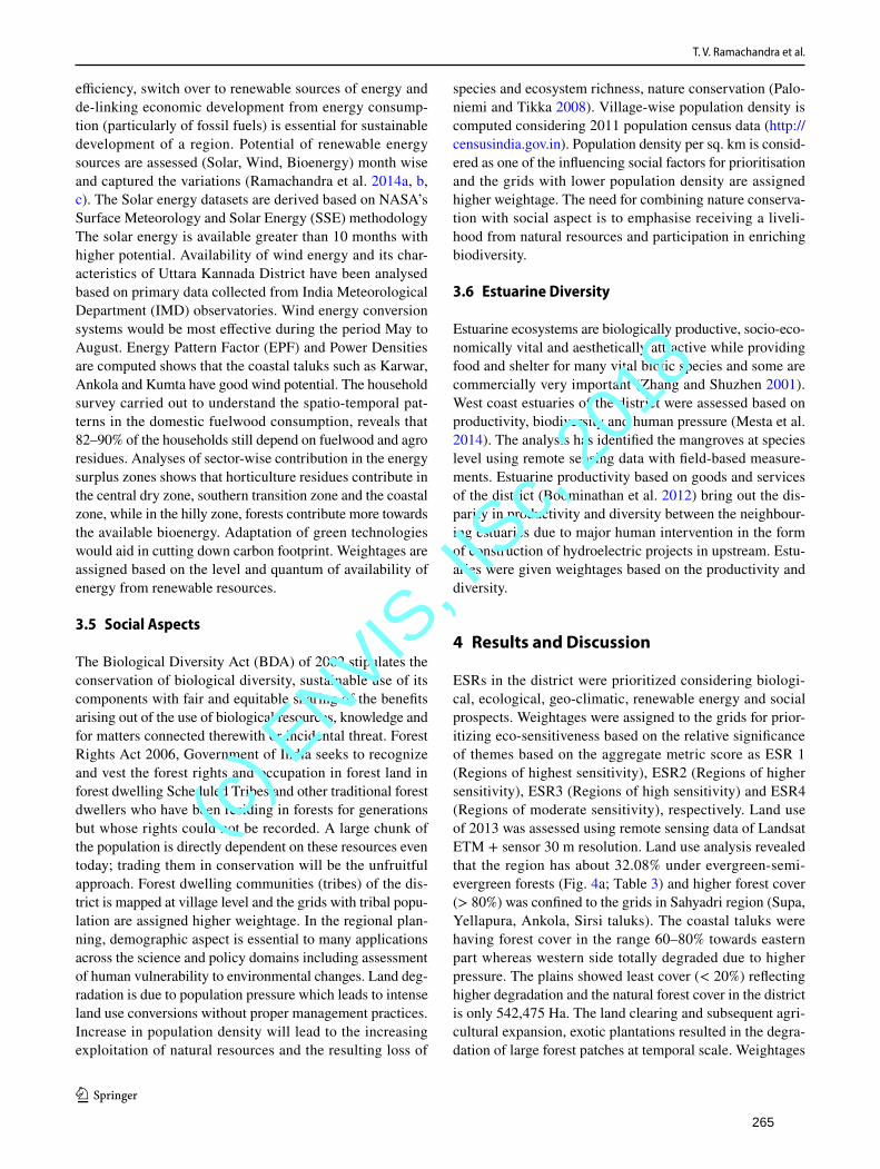
T. V. Ramachandra et al.
1 3
efficiency, switch over to renewable sources of energy and de-linking economic development from energy consump-tion (particularly of fossil fuels) is essential for sustainable development of a region. Potential of renewable energy sources are assessed (Solar, Wind, Bioenergy) month wise and captured the variations (Ramachandra et al. 2014a, b, c). The Solar energy datasets are derived based on NASA’s Surface Meteorology and Solar Energy (SSE) methodology The solar energy is available greater than 10 months with higher potential. Availability of wind energy and its char-acteristics of Uttara Kannada District have been analysed based on primary data collected from India Meteorological Department (IMD) observatories. Wind energy conversion systems would be most effective during the period May to August. Energy Pattern Factor (EPF) and Power Densities are computed shows that the coastal taluks such as Karwar, Ankola and Kumta have good wind potential. The household survey carried out to understand the spatio-temporal pat-terns in the domestic fuelwood consumption, reveals that 82–90% of the households still depend on fuelwood and agro residues. Analyses of sector-wise contribution in the energy surplus zones shows that horticulture residues contribute in the central dry zone, southern transition zone and the coastal zone, while in the hilly zone, forests contribute more towards the available bioenergy. Adaptation of green technologies would aid in cutting down carbon footprint. Weightages are assigned based on the level and quantum of availability of energy from renewable resources.
3.5 Social Aspects
The Biological Diversity Act (BDA) of 2002 stipulates the conservation of biological diversity, sustainable use of its components with fair and equitable sharing of the benefits arising out of the use of biological resources, knowledge and for matters connected therewith or incidental threat. Forest Rights Act 2006, Government of India seeks to recognize and vest the forest rights and occupation in forest land in forest dwelling Scheduled Tribes and other traditional forest dwellers who have been residing in forests for generations but whose rights could not be recorded. A large chunk of the population is directly dependent on these resources even today; trading them in conservation will be the unfruitful approach. Forest dwelling communities (tribes) of the dis-trict is mapped at village level and the grids with tribal popu-lation are assigned higher weightage. In the regional plan-ning, demographic aspect is essential to many applications across the science and policy domains including assessment of human vulnerability to environmental changes. Land deg-radation is due to population pressure which leads to intense land use conversions without proper management practices. Increase in population density will lead to the increasing exploitation of natural resources and the resulting loss of
species and ecosystem richness, nature conservation (Palo-niemi and Tikka 2008). Village-wise population density is computed considering 2011 population census data (http://censu sindi a.gov.in). Population density per sq. km is consid-ered as one of the influencing social factors for prioritisation and the grids with lower population density are assigned higher weightage. The need for combining nature conserva-tion with social aspect is to emphasise receiving a liveli-hood from natural resources and participation in enriching biodiversity.
3.6 Estuarine Diversity
Estuarine ecosystems are biologically productive, socio-eco-nomically vital and aesthetically attractive while providing food and shelter for many vital biotic species and some are commercially very important (Zhang and Shuzhen 2001). West coast estuaries of the district were assessed based on productivity, biodiversity and human pressure (Mesta et al. 2014). The analysis has identified the mangroves at species level using remote sensing data with field-based measure-ments. Estuarine productivity based on goods and services of the district (Boominathan et al. 2012) bring out the dis-parity in productivity and diversity between the neighbour-ing estuaries due to major human intervention in the form of construction of hydroelectric projects in upstream. Estu-aries were given weightages based on the productivity and diversity.
4 Results and Discussion
ESRs in the district were prioritized considering biologi-cal, ecological, geo-climatic, renewable energy and social prospects. Weightages were assigned to the grids for prior-itizing eco-sensitiveness based on the relative significance of themes based on the aggregate metric score as ESR 1 (Regions of highest sensitivity), ESR2 (Regions of higher sensitivity), ESR3 (Regions of high sensitivity) and ESR4 (Regions of moderate sensitivity), respectively. Land use of 2013 was assessed using remote sensing data of Landsat ETM + sensor 30 m resolution. Land use analysis revealed that the region has about 32.08% under evergreen-semi-evergreen forests (Fig. 4a; Table 3) and higher forest cover (> 80%) was confined to the grids in Sahyadri region (Supa, Yellapura, Ankola, Sirsi taluks). The coastal taluks were having forest cover in the range 60–80% towards eastern part whereas western side totally degraded due to higher pressure. The plains showed least cover (< 20%) reflecting higher degradation and the natural forest cover in the district is only 542,475 Ha. The land clearing and subsequent agri-cultural expansion, exotic plantations resulted in the degra-dation of large forest patches at temporal scale. Weightages
265
(c) E
NVIS, I
ISc,
2018
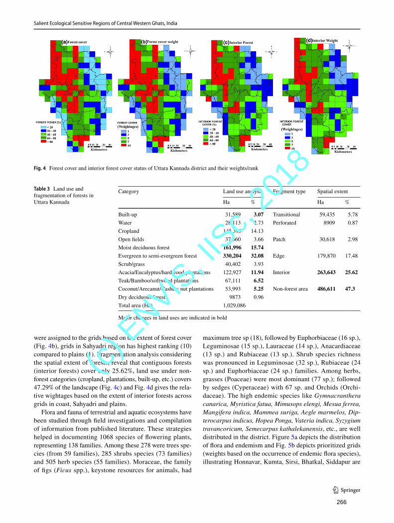
Salient Ecological Sensitive Regions of Central Western Ghats, India
1 3
were assigned to the grids based on the extent of forest cover (Fig. 4b), grids in Sahyadri region has highest ranking (10) compared to plains (1). Fragmentation analysis considering the spatial extent of forests, reveal that contiguous forests (interior forests) cover only 25.62%, land use under non-forest categories (cropland, plantations, built-up, etc.) covers 47.29% of the landscape (Fig. 4c) and Fig. 4d gives the rela-tive wightages based on the extent of interior forests across grids in coast, Sahyadri and plains.
Flora and fauna of terrestrial and aquatic ecosystems have been studied through field investigations and compilation of information from published literature. These strategies helped in documenting 1068 species of flowering plants, representing 138 families. Among these 278 were trees spe-cies (from 59 families), 285 shrubs species (73 families) and 505 herb species (55 families). Moraceae, the family of figs (Ficus spp.), keystone resources for animals, had
maximum tree sp (18), followed by Euphorbiaceae (16 sp.), Leguminosae (15 sp.), Lauraceae (14 sp.), Anacardiaceae (13 sp.) and Rubiaceae (13 sp.). Shrub species richness was pronounced in Leguminosae (32 sp.), Rubiaceae (24 sp.) and Euphorbiaceae (24 sp.) families. Among herbs, grasses (Poaceae) were most dominant (77 sp.); followed by sedges (Cyperaceae) with 67 sp. and Orchids (Orchi-daceae). The high endemic species like Gymnacranthera canarica, Myristica fatua, Mimusops elengi, Mesua ferrea, Mangifera indica, Mammea suriga, Aegle marmelos, Dip-terocarpus indicus, Hopea Ponga, Vateria indica, Syzygium travancoricum, Semecarpus kathalekanensis, etc., are well distributed in the district. Figure 5a depicts the distribution of flora and endemism and Fig. 5b depicts prioritized grids (weights based on the occurrence of endemic flora species), illustrating Honnavar, Kumta, Sirsi, Bhatkal, Siddapur are
Fig. 4 Forest cover and interior forest cover status of Uttara Kannada district and their weights/rank
Table 3 Land use and fragmentation of forests in Uttara Kannada
Major changes in land uses are indicated in bold
Category Land use analysis Fragment type Spatial extent
Ha % Ha %
Built-up 31,589 3.07 Transitional 59,435 5.78Water 28,113 2.73 Perforated 8909 0.87Cropland 145,395 14.13Open fields 37,660 3.66 Patch 30,618 2.98Moist deciduous forest 161,996 15.74Evergreen to semi-evergreen forest 330,204 32.08 Edge 179,870 17.48Scrub/grass 40,402 3.93Acacia/Eucalyptus/hardwood plantations 122,927 11.94 Interior 263,643 25.62Teak/Bamboo/softwood plantations 67,111 6.52Coconut/Arecanut/Cashew nut plantations 53,993 5.25 Non-forest area 486,611 47.3Dry deciduous forest 9873 0.96Total area (Ha) 1,029,086
266
(c) E
NVIS, I
ISc,
2018
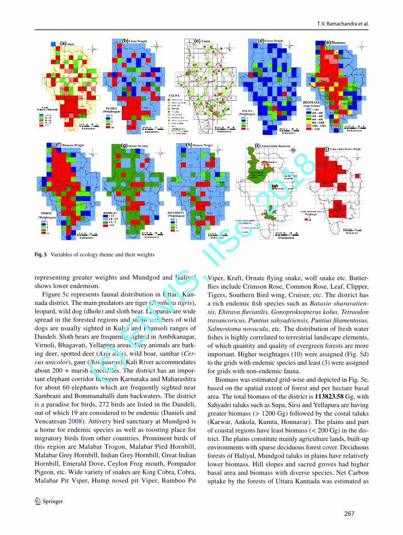
T. V. Ramachandra et al.
1 3
representing greater weights and Mundgod and Haliyal shows lower endemism.
Figure 5c represents faunal distribution in Uttara Kan-nada district. The main predators are tiger (Panthera tigris), leopard, wild dog (dhole) and sloth bear. Leopards are wide spread in the forested regions and small numbers of wild dogs are usually sighted in Kulgi and Phansoli ranges of Dandeli. Sloth bears are frequently sighted in Ambikanagar, Virnoli, Bhagavati, Yellapura areas. Prey animals are bark-ing deer, spotted deer (Axis axis), wild boar, sambar (Cer-vus unicolor), gaur (Bos gaurus). Kali River accommodates about 200 + marsh crocodiles. The district has an impor-tant elephant corridor between Karnataka and Maharashtra for about 60 elephants which are frequently sighted near Sambrani and Bommanahalli dam backwaters. The district is a paradise for birds, 272 birds are listed in the Dandeli, out of which 19 are considered to be endemic (Daniels and Vencatesan 2008). Attivery bird sanctuary at Mundgod is a home for endemic species as well as roosting place for migratory birds from other countries. Prominent birds of this region are Malabar Trogon, Malabar Pied Hornbill, Malabar Grey Hornbill, Indian Grey Hornbill, Great Indian Hornbill, Emerald Dove, Ceylon Frog mouth, Pompador Pigeon, etc. Wide variety of snakes are King Cobra, Cobra, Malabar Pit Viper, Hump nosed pit Viper, Bamboo Pit
Fig. 5 Variables of ecology theme and their weights
Viper, Kraft, Ornate flying snake, wolf snake etc. Butter-flies include Crimson Rose, Common Rose, Leaf, Clipper, Tigers, Southern Bird wing, Cruiser, etc. The district has a rich endemic fish species such as Batasio sharavatien-sis, Ehirava fluviatilis, Gonoproktopterus kolus, Tetraodon travancoricus, Puntius sahyadriensis, Puntius filamentosus, Salmostoma novacula, etc. The distribution of fresh water fishes is highly correlated to terrestrial landscape elements, of which quantity and quality of evergreen forests are more important. Higher weightages (10) were assigned (Fig. 5d) to the grids with endemic species and least (3) were assigned for grids with non-endemic fauna.
Biomass was estimated grid-wise and depicted in Fig. 5e, based on the spatial extent of forest and per hectare basal area. The total biomass of the district is 113823.58 Gg, with Sahyadri taluks such as Supa, Sirsi and Yellapura are having greater biomass (> 1200 Gg) followed by the costal taluks (Karwar, Ankola, Kumta, Honnavar). The plains and part of coastal regions have least biomass (< 200 Gg) in the dis-trict. The plains constitute mainly agriculture lands, built-up environments with sparse deciduous forest cover. Deciduous forests of Haliyal, Mundgod taluks in plains have relatively lower biomass. Hill slopes and sacred groves had higher basal area and biomass with diverse species. Net Carbon uptake by the forests of Uttara Kannada was estimated as
267
(c) E
NVIS, I
ISc,
2018
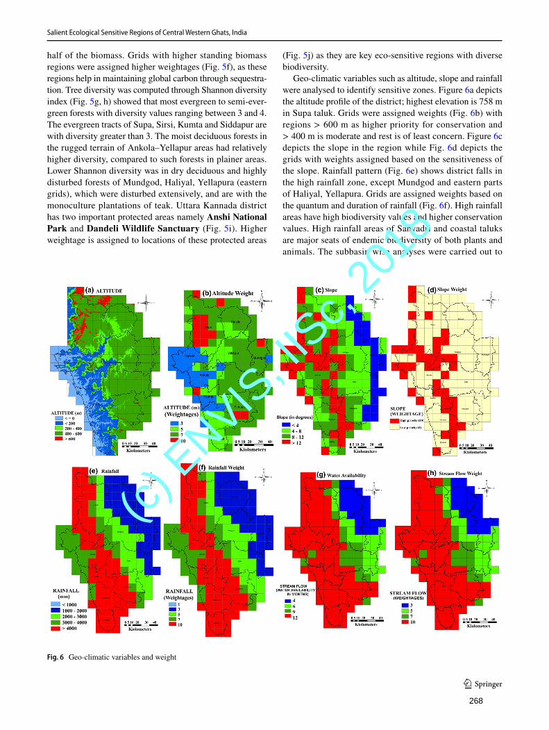
Salient Ecological Sensitive Regions of Central Western Ghats, India
1 3
half of the biomass. Grids with higher standing biomass regions were assigned higher weightages (Fig. 5f), as these regions help in maintaining global carbon through sequestra-tion. Tree diversity was computed through Shannon diversity index (Fig. 5g, h) showed that most evergreen to semi-ever-green forests with diversity values ranging between 3 and 4. The evergreen tracts of Supa, Sirsi, Kumta and Siddapur are with diversity greater than 3. The moist deciduous forests in the rugged terrain of Ankola–Yellapur areas had relatively higher diversity, compared to such forests in plainer areas. Lower Shannon diversity was in dry deciduous and highly disturbed forests of Mundgod, Haliyal, Yellapura (eastern grids), which were disturbed extensively, and are with the monoculture plantations of teak. Uttara Kannada district has two important protected areas namely Anshi National Park and Dandeli Wildlife Sanctuary (Fig. 5i). Higher weightage is assigned to locations of these protected areas
(Fig. 5j) as they are key eco-sensitive regions with diverse biodiversity.
Geo-climatic variables such as altitude, slope and rainfall were analysed to identify sensitive zones. Figure 6a depicts the altitude profile of the district; highest elevation is 758 m in Supa taluk. Grids were assigned weights (Fig. 6b) with regions > 600 m as higher priority for conservation and > 400 m is moderate and rest is of least concern. Figure 6c depicts the slope in the region while Fig. 6d depicts the grids with weights assigned based on the sensitiveness of the slope. Rainfall pattern (Fig. 6e) shows district falls in the high rainfall zone, except Mundgod and eastern parts of Haliyal, Yellapura. Grids are assigned weights based on the quantum and duration of rainfall (Fig. 6f). High rainfall areas have high biodiversity values and higher conservation values. High rainfall areas of Sahyadri and coastal taluks are major seats of endemic biodiversity of both plants and animals. The subbasin wise analyses were carried out to
Fig. 6 Geo-climatic variables and weight
268
(c) E
NVIS, I
ISc,
2018
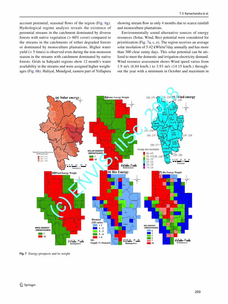
T. V. Ramachandra et al.
1 3
account perennial, seasonal flows of the region (Fig. 6g). Hydrological regime analysis reveals the existence of perennial streams in the catchment dominated by diverse forests with native vegetation (> 60% cover) compared to the streams in the catchments of either degraded forests or dominated by monoculture plantations. Higher water yield (> 5 times) is observed even during the non-monsoon season in the streams with catchment dominated by native forests. Grids in Sahyadri regions show 12 month’s water availability in the streams and were assigned higher weight-ages (Fig. 6h). Haliyal, Mundgod, eastern part of Yellapura
showing stream flow as only 4 months due to scarce rainfall and monoculture plantations.
Environmentally sound alternative sources of energy resources (Solar, Wind, Bio) potential were considered for prioritization (Fig. 7a, c, e). The region receives an average solar insolation of 5.42 kWh/m2/day annually and has more than 300 clear sunny days. This solar potential can be uti-lized to meet the domestic and irrigation electricity demand. Wind resource assessment shows Wind speed varies from 1.9 m/s (6.84 km/h.) to 3.93 m/s (14.15 km/h.) through-out the year with a minimum in October and maximum in
Fig. 7 Energy prospects and its weight
269
(c) E
NVIS, I
ISc,
2018
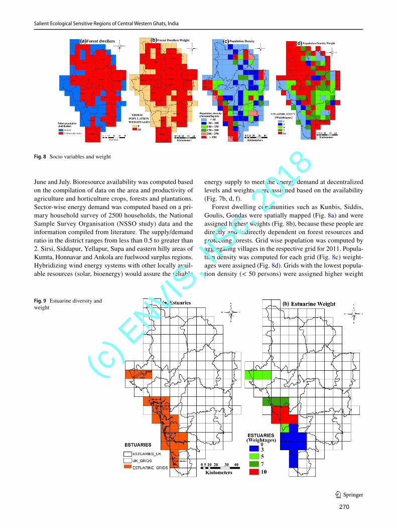
Salient Ecological Sensitive Regions of Central Western Ghats, India
1 3
June and July. Bioresource availability was computed based on the compilation of data on the area and productivity of agriculture and horticulture crops, forests and plantations. Sector-wise energy demand was computed based on a pri-mary household survey of 2500 households, the National Sample Survey Organisation (NSSO study) data and the information compiled from literature. The supply/demand ratio in the district ranges from less than 0.5 to greater than 2. Sirsi, Siddapur, Yellapur, Supa and eastern hilly areas of Kumta, Honnavar and Ankola are fuelwood surplus regions. Hybridizing wind energy systems with other locally avail-able resources (solar, bioenergy) would assure the reliable
energy supply to meet the energy demand at decentralized levels and weights were assigned based on the availability (Fig. 7b, d, f).
Forest dwelling communities such as Kunbis, Siddis, Goulis, Gondas were spatially mapped (Fig. 8a) and were assigned highest weights (Fig. 8b), because these people are directly and indirectly dependent on forest resources and protecting forests. Grid wise population was computed by aggregating villages in the respective grid for 2011. Popula-tion density was computed for each grid (Fig. 8c) weight-ages were assigned (Fig. 8d). Grids with the lowest popula-tion density (< 50 persons) were assigned higher weight
Fig. 8 Socio variables and weight
Fig. 9 Estuarine diversity and weight
270
(c) E
NVIS, I
ISc,
2018
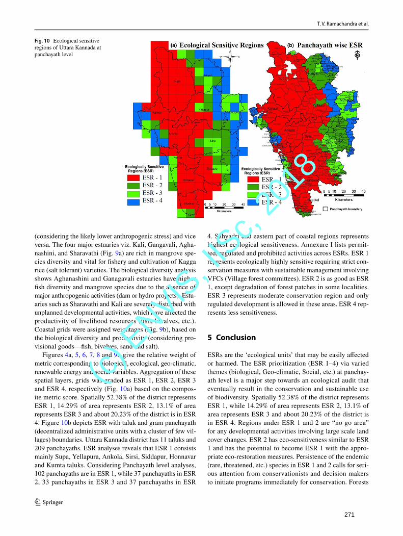
T. V. Ramachandra et al.
1 3
(considering the likely lower anthropogenic stress) and vice versa. The four major estuaries viz. Kali, Gangavali, Agha-nashini, and Sharavathi (Fig. 9a) are rich in mangrove spe-cies diversity and vital for fishery and cultivation of Kagga rice (salt tolerant) varieties. The biological diversity analysis shows Aghanashini and Ganagavali estuaries have higher fish diversity and mangrove species due to the absence of major anthropogenic activities (dam or hydro projects). Estu-aries such as Sharavathi and Kali are severely disturbed with unplanned developmental activities, which have affected the productivity of livelihood resources (fish, bivalves, etc.). Coastal grids were assigned weightages (Fig. 9b), based on the biological diversity and productivity (considering pro-visional goods—fish, bivalves, sand and salt).
Figures 4a, 5, 6, 7, 8 and 9b give the relative weight of metric corresponding to biological, ecological, geo-climatic, renewable energy and social variables. Aggregation of these spatial layers, grids was graded as ESR 1, ESR 2, ESR 3 and ESR 4, respectively (Fig. 10a) based on the compos-ite metric score. Spatially 52.38% of the district represents ESR 1, 14.29% of area represents ESR 2, 13.1% of area represents ESR 3 and about 20.23% of the district is in ESR 4. Figure 10b depicts ESR with taluk and gram panchayath (decentralized administrative units with a cluster of few vil-lages) boundaries. Uttara Kannada district has 11 taluks and 209 panchayaths. ESR analyses reveals that ESR 1 consists mainly Supa, Yellapura, Ankola, Sirsi, Siddapur, Honnavar and Kumta taluks. Considering Panchayath level analyses, 102 panchayaths are in ESR 1, while 37 panchayaths in ESR 2, 33 panchayaths in ESR 3 and 37 panchayaths in ESR
4. Sahyadri and eastern part of coastal regions represents highest ecological sensitiveness. Annexure I lists permit-ted, regulated and prohibited activities across ESRs. ESR 1 represents ecologically highly sensitive requiring strict con-servation measures with sustainable management involving VFCs (Village forest committees). ESR 2 is as good as ESR 1, except degradation of forest patches in some localities. ESR 3 represents moderate conservation region and only regulated development is allowed in these areas. ESR 4 rep-resents less sensitiveness.
5 Conclusion
ESRs are the ‘ecological units’ that may be easily affected or harmed. The ESR prioritization (ESR 1–4) via varied themes (biological, Geo-climatic, Social, etc.) at panchay-ath level is a major step towards an ecological audit that eventually result in the conservation and sustainable use of biodiversity. Spatially 52.38% of the district represents ESR 1, while 14.29% of area represents ESR 2, 13.1% of area represents ESR 3 and about 20.23% of the district is in ESR 4. Regions under ESR 1 and 2 are “no go area” for any developmental activities involving large scale land cover changes. ESR 2 has eco-sensitiveness similar to ESR 1 and has the potential to become ESR 1 with the appro-priate eco-restoration measures. Persistence of the endemic (rare, threatened, etc.) species in ESR 1 and 2 calls for seri-ous attention from conservationists and decision makers to initiate programs immediately for conservation. Forests
Fig. 10 Ecological sensitive regions of Uttara Kannada at panchayath level
271
(c) E
NVIS, I
ISc,
2018
Salient Ecological Sensitive Regions of Central Western Ghats, India
1 3
with innumerable streams (i.e., water course forests) in the Western Ghats, offer tremendous potential for carbon stocking per unit area while also bettering the hydrology of these mountains, which form the main watershed for the entire Indian peninsula. These water course forests are not only rich with biodiversity, but are also with high biomass, which highlights the greater carbon sequestration potential and their prime role towards mitigation of impacts of global warming. This emphasizes the need for the review of exist-ing forest policies to ensure sustenance of ecological ser-vices through the sustainable forest management strategies. Millions of subsistence farmers and other forest dwellers of Western Ghats can not only be partners in micro-level plan-ning for prudent water use, but also stand to gain in a big way from carbon credits for their new role as promoters and guardians of watershed vegetation. Rendering such service for mitigating global climatic change can also, same time, serve well the cause of eco-sensitive regions in an otherwise much impacted biodiversity hotspot. The premium should be on conservation of the remaining ecologically sensitive regions, which are vital for the water security (perenniality of streams), mitigation of global carbon and food security (sustenance of biodiversity). There still exists a chance to restore the lost natural evergreen to semi-evergreen forests in the Western Ghats region through appropriate conservation and management practices. The management of biodiversity hotspot regions should focus on the conservation as well as socio-economic developmental aspects.
These ESRs or eco-clusters approach aids in the con-servation of ecology, biodiversity, water resources, culture and traditions while paving way for location specific eco-nomic development, primarily aimed at elevating levels of
livelihood security. ESRs are seen in the context of sustain-ability and environmental friendly behavior as means for a socio-ecological transition in the long run. The eco-clusters at decentralized levels aid as driver for conservation of eco-logically sensitive regions and implementation of an appro-priate regional economic policy with the necessary incen-tive structures to foster eco-innovation as well as growth and employment at local levels (with the region specific industries such as agro processing, etc.). This envisage the foundation of an on-going process to integrate ecological and environmental considerations into administration in the ecologically fragile and biodiversity rich districts of Western Ghats. The integrated database on biodiversity and socio processes furnishes analyzed data, advice and management prescriptions to beneficiaries at every level from the village communities to the Government. It is shown that eco-clus-ters are crucial for a sustainable development and thus need political commitment and incentives for the development of eco-industry sector (based on the local renewable natural resources). Thus, ESRs will aid as catalysts in a well-ordered decision making process through stake holder’s active par-ticipation with the priorities for sustainable livelihood.
Acknowledgement We are grateful to (i) ENVIS Division, the Minis-try of Environment, Forests and Climate Change, Government of India, (ii) NRDMS Division, the Ministry of Science and Technology (DST), Government of India, (iii) Karnataka Biodiversity Board, Western Ghats Task Force, Government of Karnataka and (iv) Indian Institute of Science for the financial and infrastructure support. We acknowledge the support of Karnataka Forest Department for giving necessary per-missions to undertake ecological research in Central Western Ghats. We thank Vishnu Mukri and Srikanth Naik for the assistance during field data collection.
272
(c) E
NVIS, I
ISc,
2018
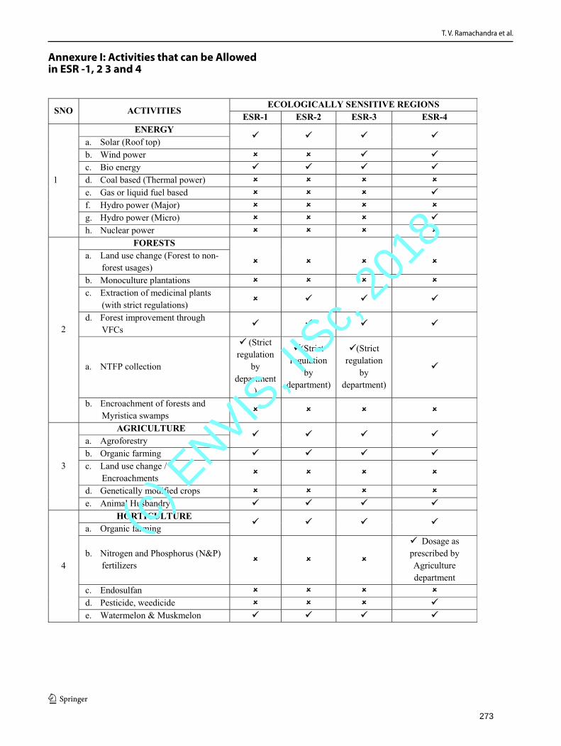
T. V. Ramachandra et al.
1 3
Annexure I: Activities that can be Allowed in ESR ‑1, 2 3 and 4
273
(c) E
NVIS, I
ISc,
2018
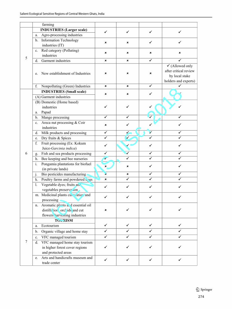
Salient Ecological Sensitive Regions of Central Western Ghats, India
1 3274
(c) E
NVIS, I
ISc,
2018
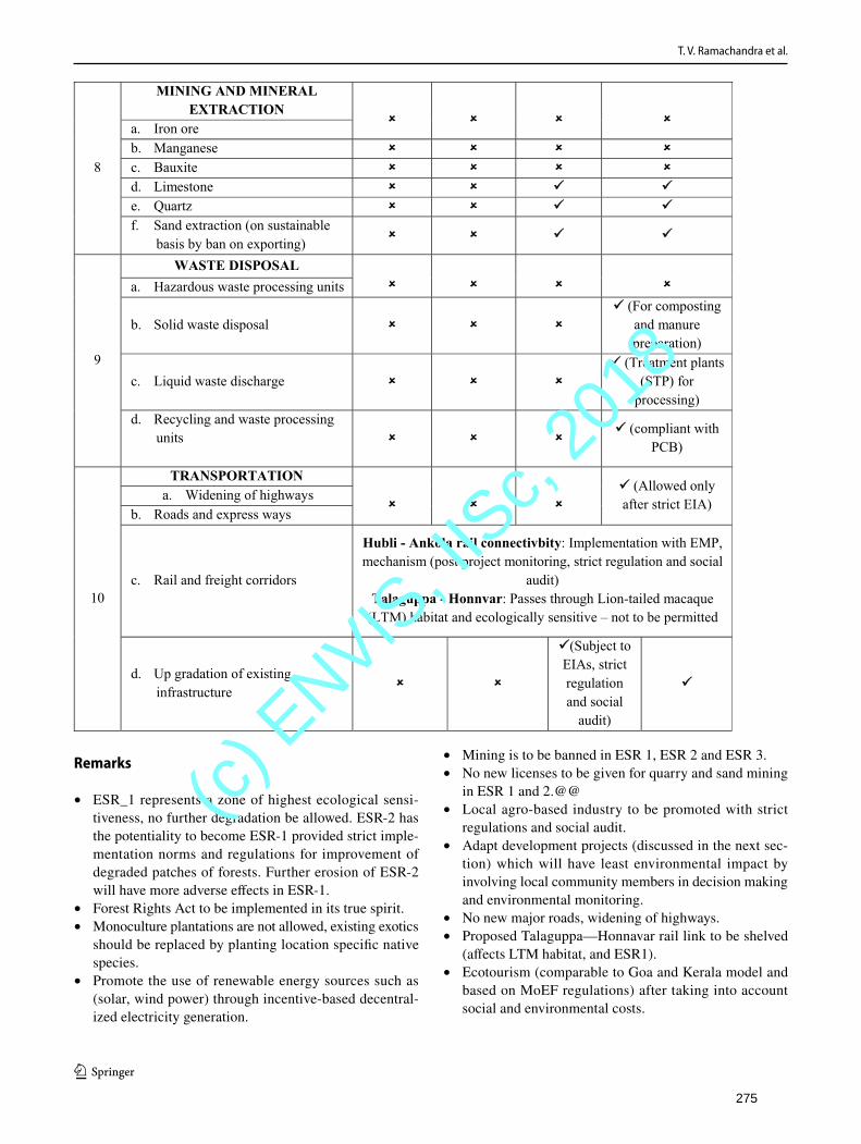
T. V. Ramachandra et al.
1 3
Remarks
• ESR_1 represents a zone of highest ecological sensi-tiveness, no further degradation be allowed. ESR-2 has the potentiality to become ESR-1 provided strict imple-mentation norms and regulations for improvement of degraded patches of forests. Further erosion of ESR-2 will have more adverse effects in ESR-1.
• Forest Rights Act to be implemented in its true spirit.• Monoculture plantations are not allowed, existing exotics
should be replaced by planting location specific native species.
• Promote the use of renewable energy sources such as (solar, wind power) through incentive-based decentral-ized electricity generation.
• Mining is to be banned in ESR 1, ESR 2 and ESR 3.• No new licenses to be given for quarry and sand mining
in ESR 1 and 2.@@• Local agro-based industry to be promoted with strict
regulations and social audit.• Adapt development projects (discussed in the next sec-
tion) which will have least environmental impact by involving local community members in decision making and environmental monitoring.
• No new major roads, widening of highways.• Proposed Talaguppa—Honnavar rail link to be shelved
(affects LTM habitat, and ESR1).• Ecotourism (comparable to Goa and Kerala model and
based on MoEF regulations) after taking into account social and environmental costs.
275
(c) E
NVIS, I
ISc,
2018
Salient Ecological Sensitive Regions of Central Western Ghats, India
1 3
• The laterite formations are aesthetically pleasing, and particularly with the massive flowering of rainy season herbs. The terrain is ideal for tourism and scientific stud-ies.
References
Beinat E (1997) Value functions for environmental management. Klu-wer Academic, Boston, p 241
Berkres F, Davidson-Hunt IJ (2006) Biodiversity, traditional manage-ment systems, and cultural landscapes: examples from the boreal forest of Canada. Int Soc Sci J 58:35–47
Blicharska M, Orlikowska EH, Roberge JM, Grodzinska-Jurczak M (2016) Contribution of social science to large scale biodiversity conservation: a review of research about the natura 2000 network. Biol Cons 199:110–122
Bourne A, Holness S, Holden P, Scorgie S, Donatti CI, Midgley G (2016) A Socio-Ecological Approach for Identifying and Con-textualising Spatial Ecosystem-Based Adaptation Priorities at the Sub-National Level. PLoS ONE 11(5):e0155235
Boyd C, Brooks TM, Butchart SH, Edgar GJ, Da Fonseca GA, Hawk-ins F, Hoffmann M, Sechrest W, Stuart SN, Van Dijk PP (2008) Spatial scale and the conservation of threatened species. Conserv Lett 1(1):37–43
Brose U, Martinez ND, Williams RJ (2003) Estimating species rich-ness: sensitivity to sample coverage and insensitivity to spatial patterns. Ecology 84:2364–2377
Brown S (1997) Estimating biomass and biomass change of tropical forests: a primer, FAO Forestry Paper, 134
Burrough PA, McDonell RA (1998) Principles of Geographical Infor-mation Systems. Oxford University Press, New York, p 190
Calder IR (2012) Forests and hydrological services: reconciling public and science perceptions. Land Use Water Resour Res 2(2):21–212
Boominathan M, Ravikumar G, Chandran, MDS, Ramachandra TV (2012) The impact of dams on the edible bivalves–a compara-tive study of Kali and Aghanashini Estuaries of Uttara Kan-nada District, Karnataka, India. In: Ramanathan AL, Sreekesh S, Sundararajan M (eds) The proceedings of national conference on mangrove wetlands and near shore marine ecosystems from sustainability issues to management and restoration. pp 45–46
Conradin K, Hammer T (2016) Making the most of world natural herit-age—linking conservation and sustainable regional development? Sustainability 8(4):323
Daniels RJR, Vencatesan J (2008) Western Ghats: biodiversity, people conservation. Rupa & Co, New Delhi
de Lima RF, Dallimer M, Atkinson PW, Barlow J (2013) Biodiversity and land-use change: understanding the complex responses of an endemic-rich bird assemblage. Divers Distrib 19(4):411–422
Gadgil M, Daniels RJR, Ganeshaiah KN, Prasad SN, Murthy MSR, Jha CS, Ramesh BR, Subramaniam KA (2011) Mapping ecologically sensitive, significant and salient areas of Western Ghats: proposed protocol and methodology. Curr Sci 100(2):175–182
Kibert CJ, Thiele L, Peterson A, Monroe M (2011) The ethics of sus-tainability. John Wiley & Sons Ltd, UK
Kivinen S, Kumpula T (2013) Detecting land cover disturbances in the Lappi reindeer herding district using multi-source remote sens-ing and GIS data. Int J Appl Earth Obs Geo Inf 27:13–19 (ISSN 0303-2434)
Knight AT, Cowling RM, Campbell BM (2006) An operational model for implementing conservation action. Conserv Biol 20:408–419
Levin N, Watson JE, Joseph LN, Grantham HS, Hadar L, Apel N, Perevolotsky A, DeMalach N, Possingham HP, Kark S (2013) A
framework for systematic conservation planning and management of Mediterranean landscapes. Biol Cons 158:371–383
Li A, Wang A, Liang S, Zhou W (2006) Eco-environmental vulner-ability evaluation in mountainous region using remote sensing and GIS-a case study in the upper reaches of Minjiang River, China. Ecol Model 192:175–187
Lou J (2006) Entropy and diversity. Oikos 113(2):363–375Margules C, Pressey R (2000) Systematic conservation planning.
Nature 405:243–253Marignani M, Blasi C (2012) Looking for important plant areas: selec-
tion based on criteria, complementarity, or both? Biodivers Con-serv 21:1853–1864
Mesta PN, Setturu B, Chandran MDS, Rajan KS, Ramachandra TV (2014) Inventorying, mapping and monitoring of mangroves towards sustainable management of West Coast, India. J Geophys Remote Sens 3:130. https ://doi.org/10.4172/2169-0049.10001 30
Moen J, Keskitalo EC (2010) Interlocking panarchies in multi-use boreal forests in Sweden. Ecol Soc 15(3):17
Myers N, Mittermeier RA, Mittermeier CG, Da Fonseca GA, Kent J (2000) Biodiversity hotspots for conservation priorities. Nature 403(6772):853–858
Nagasaka A, Futoshi N (1999) The influences of land-use changes on hydrology and riparian environment in a northern Japanese landscape. Landscape Ecol 14:543–556
Opdam P, Steingröver E, Van Rooij S (2006) Ecological networks: a spatial concept for multi-actor planning of sustainable landscapes. Landsc Urban Plan 75(3):322–332
Paloniemi R, Tikka PM (2008) Ecological and social aspects of biodiversity conservation on private lands. Environ Sci Policy 11(4):336–346
Peterson AT, Egbert SL, Cordero VS, Price KP (2000) Geographic analysis of conservation priority: endemic birds and mammals in Veracruz, Mexico. Biol Cons 93(1):85–94
Pressey RL, Cabeza M, Watts ME, Cowling RM, Wilson KA (2007) Conservation planning in a changing world. Trends Ecol Evol 22(11):583–592
Ramachandra TV (2014) Hydrological responses at regional scale to landscape dynamics. J Biodivers 5(1-2):11–32
Ramachandra TV, Joshi NV, Subramanian DK (2000) Present and prospective role of bio-energy in regional energy system. Renew Sustain Energy Rev 4:375–430
Ramachandra TV, Chandran MDS, Gururaja KV, Sreekantha (2007) Cumulative environmental impact assessment. Nova Science Pub-lishers, New York
Ramachandra TV, Hegde G, Das GK (2014a) Scope of solar energy in Uttara Kannada, Karnataka State, India: roof top PV for domes-tic electricity and standalone systems for irrigation. Productivity 55(1):100
Ramachandra TV, Hegde G, Krishnadas G (2014b) Potential assess-ment and decentralized applications of wind energy in Uttara Kan-nada, Karnataka. Int J Renew Energy Res 4(1):1
Ramachandra TV, Hegde G, Setturu B, Krishnadas G (2014c) Bio-energy: a sustainable energy option for rural India. Adv For Lett (AFL) 3(1):1–5
Ramachandra TV, Chandran MDS, Rao GR, Mukri Vishnu, Joshi NV (2015) Floristic diversity in Uttara Kannada district, Karna-taka. In: Pullaiah T, Sandhya R (eds) Biodiversity in India, vol 8. Regency Publications, New Delhi, pp 1–87
Ramachandra TV, Setturu B, Chandran S (2016) Geospatial analy-sis of forest fragmentation in Uttara Kannada District, India. For Ecosyst 3(1):10
Riitters KH, Wickham JD, Coulston JW (2004) A preliminary assess-ment of Montréal process indicators of forest fragmentation for the United States. Environ Monit Assess 91:257–276
276
(c) E
NVIS, I
ISc,
2018
T. V. Ramachandra et al.
1 3
Rouget M, Cowling RM, Lombard AT, Knight AT, Kerley GI (2006) Designing large-scale conservation corridors for pattern and pro-cess. Conserv Biol 20(2):54
Sen P (2000) Report of The Committee on Identifying Parameters for Designating Ecologically Sensitive Areas in India. Ministry of Environment and Forests, Government of India, New Delhi
Termorshuizen JW, Opdam P (2009) Landscape services as a bridge between landscape ecology and sustainable development. Land-scape Ecol 24(8):1037–1052
Toth S, Haight RG, Rogers L (2011) Dynamic reserve selection, optimal land retention with land price feedbacks. Oper Res 59(5):1059–1078
Vigl LE, Schirpke U, Tasser E, Tappeiner U (2016) Linking long-term landscape dynamics to the multiple interactions among ecosystem services in the European Alps. Landscape Ecol 31:1–6
Vinay S, Bharath S, Bharath HA, Ramachandra TV (2013) Hydro-logic model with landscape dynamics for drought monitoring. In: Proceeding of joint international workshop of ISPRS WG VIII/1 and WG IV/4 on geospatial data for disaster and risk reduction, Hyderabad, November 2013, pp. 21–22
Wang X, Zhong X, Gao P (2010) A GIS-based decision support system for regional eco-security assessment and its application on the Tibetan Plateau. J Environ Manage 91:1981–1990
Wasige JE, Thomas AG, Smaling E, Victor J (2013) Monitoring basin-scale land cover changes in Kagera Basin of Lake Victoria using
ancillary data and remote sensing. Int J Appl Earth Obs Geoinf 21:32–42
Watson JEM, Grantham H, Wilson KA, Possingham HP (2011a) Systematic conservation planning: past, present and future. In: Whittaker R, Ladle R (eds) Conservation Biogeograph. Wiley-Blackwell, Oxford, pp 136–160
Watson JEM, Cross M, Rowland E, Joseph LN, Rao M, Seimon A (2011b) Planning for species conservation in a time of climate change Climate change, research and technology for climate change adaptation and mitigation, vol 3. InTech Publishers, Lon-don, pp 379–402 (ISBN: 979-953-307-278-3)
Wondie M, Schneider W, Melesse AM, Teketay D (2011) Spatial and temporal land cover changes in the Simen Mountains National Park, a world heritage site in northwestern Ethiopia. Remote Sens 3(4):752–766
Wondie M, Teketay D, Melesse AM, Schneider W (2012) Relationship between topographic variables and land cover in the Simen Moun-tains National Park, a world heritage site in northern Ethiopia. Int J Remote Sens Appl 2(2):3
Zhang Q, Shuzhen S (2001) The mangrove wetland resources and their conservation in China. J Nat Resour 16(1):28–36
277
(c) E
NVIS, I
ISc,
2018
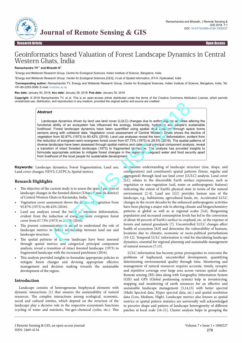
Geoinformatics based Valuation of Forest Landscape Dynamics in CentralWestern Ghats, IndiaRamachandra TV1* and Bharath S2
1Energy and Wetlands Research Group, Centre for Ecological Sciences, Indian Institute of Science, Bangalore, India2Energy and Wetlands Research Group, Center for Ecological Sciences [CES], d Lab of Spatial Informatics, IIIT-H, Hyderabad, India*Corresponding author: Ramachandra TV, Energy and Wetlands Research Group, Centre for Ecological Sciences, Indian Institute of Science, Bangalore, India, Tel:+91-80-2293-3099; E-mail: [email protected]
Rec date: January 05, 2018; Acc date: January 29, 2018; Pub date: January 30, 2018
Copyright: © 2018 Ramachandra TV, et al. This is an open-access article distributed under the terms of the Creative Commons Attribution License, which permitsunrestricted use, distribution, and reproduction in any medium, provided the original author and source are credited.
Abstract
Landscape dynamics driven by land use land cover (LULC) changes due to anthropogenic activities altering thefunctional ability of an ecosystem has influenced the ecology, biodiversity, hydrology and people’s sustainablelivelihood. Forest landscape dynamics have been quantified using spatial data acquired through space bornesensors along with collateral data. Vegetation cover assessment of Central Western Ghats shows the decline ofvegetation from 92.87% (1973) to 80.42% (2016). Land use analyses reveal the trend of deforestation, evident fromthe reduction of evergreen-semi evergreen forest cover from 67.73% (1973) to 29.5% (2016). The spatial patterns ofdiverse landscape have been assessed through spatial metrics and categorical principal component analysis, reveala transition of intact forested landscape (1973) to fragmented landscape. The analysis has provided insights toformulate appropriate policies to mitigate forest changes in the region to safeguard water and food security apartfrom livelihood of the local people for sustainable development.
Keywords: Landscape dynamics; Forest fragmentation; Land use;Land cover changes; NDVI; CATPCA; Spatial metrics
Research Highlights• The objective of the current study is to assess the spatial patterns of
landscape changes in the forested district (Uttara Kannada district)of Central Western Ghats in Karnataka, India.
• Vegetation cover assessment shows the decline of vegetation from92.87% (1973) to 80.42% (2016).
• Land use analyses reveal the trend of intensive deforestation,evident from the reduction of evergreen-semi evergreen forestcover from 67.73% (1973) to 29.5% (2016).
• The present communication is aimed to understand the role oflandscape metrics to define relationship between land use andlandscape structure.
• The spatial patterns of diverse landscape have been assessedthrough spatial metrics and categorical principal componentanalysis; reveal a transition of intact forested landscape (1973) tofragmented landscape with the increased patchiness (2016).
• This analysis provided insights to formulate appropriate policies tomitigate forest changes and devising appropriate effectivemanagement and decision making towards the sustainabledevelopment of the region.
IntroductionLandscape consists of heterogeneous biophysical elements with
dynamic interactions [1] that ensures the sustainability of naturalresources. The complex interactions among ecological, economic,social and cultural entities, which depend on the structure of thelandscape play a decisive role in the respective ecosystem’s functions(cycling of water and nutrients, bio-geo-chemical cycles, etc.). This
necessitates understanding of landscape structure (size, shape, andconfiguration) and constituent’s spatial patterns (linear, regular andaggregated) through land use land cover [LULC] analysis. Land cover[LC] relates to the discernible Earth surface expressions, such asvegetation or non-vegetation (soil, water or anthropogenic features)indicating the extent of Earth’s physical state in terms of the naturalenvironment [2-4]. Land use [LU] provides human uses of thelandscape, e.g., habitations, agricultural lands, etc. Accelerated LULCchanges in the recent decades by the enhanced anthropogenic activitieshave been playing a major role in altering climate and biogeochemistrypatterns at global as well as at regional scales [5,6]. Burgeoningpopulation and increased consumption levels has led to the conversionof about 40 percent of Earth's surface to cropland, etc. at the expense offorests and natural grasslands [7]. Uncontrolled LULC changes affecthealth of ecosystem [8,9] and determine the vulnerability of humans,locations due to climatic, economic or socio-political perturbations[10-12]. Temporal LULC information is vital for elucidating landscapedynamics, essential for regional planning and sustainable managementof natural resources [7,13].
LULC information has become prime prerequisites to overcome theproblems of haphazard, uncontrolled development, quantifyingdeteriorating environmental quality through time. Monitoring andmanagement of natural resources requires accurate, timely, synopticand repetitive coverage over large area across various spatial scales.Remote sensing (RS) data along with Geographic Information System(GIS) and GPS (Global positioning system) help in inventorying,mapping and monitoring of earth resources for an effective andsustainable landscape management [3,14,15] with better spectral(Multi Spectral data, Hyper spectral data, etc.) and spatial resolutiondata (Low, Medium, High). Landscape metrics also known as spatialmetrics or spatial pattern statistics are universally well acknowledgedto perceive shape and pattern of landscape heterogeneity of differentpatches at local scale [16-21]. Cluster analysis helps in grouping the
Jour
nal o
f Remote Sensing & G
IS
ISSN: 2469-4134 Journal of Remote Sensing & GISRamachandra and Bharath, J Remote Sensing &
GIS 2018, 7:1DOI: 10.4172/2469-4134.1000227
Research Article Open Access
J Remote Sensing & GIS, an open access journalISSN: 2469-4134
Volume 7 • Issue 1 • 1000227278
(c) E
NVIS, I
ISc,
2018
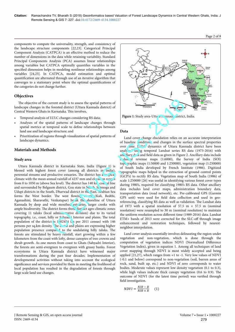
components to compute the universality, strength, and consistency ofthe landscape structure components [22,23]. Categorical PrincipalComponent Analysis (CATPCA) is an effective method to reduce thenumber of dimensions in the data while retaining variability. StandardPrincipal Components Analysis (PCA) assumes linear relationshipsamong variables but CATPCA optimally quantifies variables in thespecified dimension helps in modeling nonlinear relationships amongvariables [24,25]. In CATPCA, model estimation and optimalquantification are alternated through use of an iterative algorithm thatconverges to a stationary point where the optimal quantifications ofthe categories do not change further.
ObjectivesThe objective of the current study is to assess the spatial patterns of
landscape changes in the forested district (Uttara Kannada district) ofCentral Western Ghats in Karnataka. This involves,
• Temporal analysis of LULC changes considering RS data;• Analyses of the spatial patterns of landscape changes through
spatial metrics at temporal scale to define relationships betweenland use and landscape structure; and
• Prioritization of regions through visualization of spatial patterns oflandscape dynamics.
Materials and Methods
Study areaUttara Kannada district in Karnataka State, India (Figure 1) is
blessed with highest forest cover (among all districts in India),perennial streams and productive estuaries. The district has a tropicalclimate with the mean annual rainfall of 4237 mm and elevation rangesfrom 0 to 1050 m (above Sea level). The district has 140 km coastal lineand surrounded by Belgaum district, Goa state in North, Shimoga andUdupi districts in the South, Dharwad district in the East, Arabian Seaforms the West border. The west flowing rivers (Kali, Bedthi,Aganashini, Sharavathi, Venkatapur) break the shoreline of UttaraKannada by deep and wide mouthed estuaries, larger creeks withample biodiversity. The district forms three distinct agro climatic zonescovering 11 taluks (local administrative division) due to its variedtopography, i.e., coast, hilly or Sahyadri Interior and plains. The totalpopulation of the district is 1502454 (as per 2011 census) with 146persons per sq.km density. The costal and plains are expressing higherpopulation presence compared to the undulating hilly taluks. Theforests are stimulated by heavy rainfall, start growing within a fewkilometers from the coast with lofty, dense canopies of tree crowns andshrub growth. As one moves from coast to Ghats (Sahyadri Interior),the forests are semi-evergreen to evergreen with grassy banks. Forestecosystems in Uttara Kannada district have witnessed majortransformations during the past four decades. Implementation ofdevelopmental activities without taking into account the ecologicalsignificance and services provided by them in meeting the livelihood oflocal population has resulted in the degradation of forests throughlarge scale land use changes.
Figure 1: Study area-Uttara Kannada district, India.
DataLand cover change elucidation relies on an accurate interpretation
of baseline conditions and changes in the surface spectral propertiesover time. LULC dynamics of Uttara Kannada district have beenanalyzed using temporal Landsat series RS data (1973-2016) withancillary data and field data as given in Figure 2. Ancillary data includecadastral revenue maps (1:6000), the Survey of India (SOI)topographic maps (1:50000 and 1:250000), vegetation map (1:250000)of South India developed by French Institute (1986). Digitizedtopographic maps helped in the extraction of ground control points(GCP’s) to rectify RS data. Vegetation map of South India (1986) ofscale 1:250000 [26] was useful in identifying various forest cover typesduring 1980’s, required for classifying 1980’s RS data. Other ancillarydata includes land cover maps, administration boundary data,transportation data (road network), etc. Pre-calibrated GPS (GarminGPS unit) were used for field data collection and used in geo-referencing, classifying RS data as well as validation. The Landsat dataof 1973 with a spatial resolution of 57.5 m × 57.5 m (nominalresolution) were resampled to 30 m (nominal resolution) to maintainthe uniform resolution across different time (1989-2016) data. LandsatETM+ bands of 2013 were corrected for the SLC-off through imageenhancement and restoration techniques, followed by nearest-neighbor interpolation.
Land cover analysis essentially involves delineating the region undervegetation and non-vegetation, which is done through thecomputation of vegetation indices NDVI (Normalized DifferenceVegetation Index), given in equation 1. Among all techniques of landcover mapping through NDVI is most widely accepted and beingapplied [21,27], which ranges from +1 to -1. Very low values of NDVI(-0.1 and below) correspond to non-vegetation (soil, barren areas ofrock, sand, built up, etc.) and NDVI of zero corresponds to waterbodies. Moderate values represent low density vegetation (0.1 to 0.3),while high values indicate thick canopy vegetation (0.6 to 0.9). Theoutcome of NDVI (for the latest time period) was verified throughfield investigation.���� = ��� − ����+ � (1)
Citation: Ramachandra TV, Bharath S (2018) Geoinformatics based Valuation of Forest Landscape Dynamics in Central Western Ghats, India. JRemote Sensing & GIS 7: 227. doi:10.4172/2469-4134.1000227
Page 2 of 8
J Remote Sensing & GIS, an open access journalISSN: 2469-4134
Volume 7 • Issue 1 • 1000227279
(c) E
NVIS, I
ISc,
2018
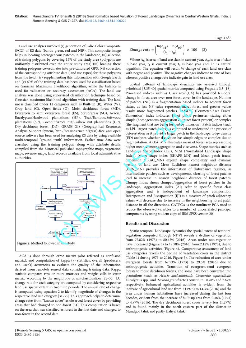
Land use analyses involved (i) generation of False Color Composite(FCC) of RS data (bands–green, red and NIR). This composite imagehelps in locating heterogeneous patches in the landscape, (ii) selectionof training polygons by covering 15% of the study area (polygons areuniformly distributed over the entire study area) (iii) loading thesetraining polygons co-ordinates into pre-calibrated GPS, (vi) collectionof the corresponding attribute data (land use types) for these polygonsfrom the field, (iv) supplementing this information with Google Earthand (v) 60% of the training data has been used for classification basedon Gaussian Maximum Likelihood algorithm, while the balance isused for validation or accuracy assessment (ACA). The land useanalysis was done using supervised classification technique based onGaussian maximum likelihood algorithm with training data. The landuse is classified under 11 categories such as Built-up (B), Water (W),Crop land (C), Open fields (O), Moist deciduous forest (MD),Evergreen to semi evergreen forest (ES), Scrub/grass (SG), Acacia/Eucalyptus/Hardwood plantations (HP), Teak/Bamboo/Softwoodplantations (SP), Coconut/Areca nut/Cashew nut plantations (CP),Dry deciduous forest (DD). GRASS GIS (Geographical ResourcesAnalysis Support System, http://ces.iisc.ernet.in/grass)-free and opensource software has been used for analyzing RS data by using availablemulti-temporal “ground truth” information. Earlier time data wereclassified using the training polygon along with attribute detailscompiled from the historical published topographic maps, vegetationmaps, revenue maps, land records available from local administrativeauthorities.
Figure 2: Method followed in the study.
ACA is done through error matrix (also referred as confusionmatrix), and computation of kappa (κ) statistics, overall (producer'sand user's) accuracies to evaluate the quality of the informationderived from remotely sensed data considering training data. Kappastatistic compares two or more matrices and weighs cells in errormatrix according to the magnitude of misclassification [28-30]. LUchange rate for each category are computed by considering respectiveland use spatial extent in two time periods. The annual rate of changeis computed using equation 2 to identify magnitude of changes in therespective land use category [31-33]. This approach helps to determinechange rates from “known cover” as observed forest cover by providingareas that had changed to non-forest [34]. This computation is basedon the area that was classified as forest in the first date and changed tonon-forest in the second date.
�ℎ���� ���� = ln(��1)− ln(��0)(�1− �0) × 100 (2)Where At1 is area of land use class in current year, At0 is area of class
in base year, t1 is current year, t0 is base year and Ln is naturallogarithm. The equation will result % change of each land use classwith negate and positive. The negative changes indicate to rate of loss;whereas positive change rate indicate gain in land use class.
Spatial patterns of landscape dynamics are assessed throughprioritised [3,35-40] spatial metrics computed using Fragstats 3.3 [16].Prioritised indices such as Class area (CA) has provided temporalchange in forest area over non-forest cover in the landscape. Numberof patches (NP) is a fragmentation based indices to account foreststatus, as less NP value represents intact forest and greater valuesresults more fragmented patches. PAFRAC (Perimeter-Area FractalDimension) index indicates forest patch perimeter, stating eithersimple (homogeneous aggregation or intact forest present) or complex(the fragment that are being formed by intrusion). Patch indices (suchas LPI- largest patch index) is computed to understand the process ofdeforestation as it provides larger patch in the landscape. Edge density(ED) analyses whether the region has simple edges or complex due tofragmentation. AREA_MN illustrates mean of forest area representinghigher mean as more aggregation and vice versa. Shape metrics such asLandscape Shape Index (LSI), NLSI (Normalized Landscape ShapeIndex), Mean shape index (SHAPE_MN) and Mean patch fractaldimension (FRAC_MN) explain shape complexity and dynamicpattern of land use. Mean Euclidean nearest neighbour distance(ENN_MN) provides the information of disturbance regimes, asintermediate patches such as developments, clearing of forest patcheslead to increase in nearest neighbour distance of forest patches.Clumpy Index shows clumped/aggregation of forest patches in thelandscape, Aggregation index (AI) refer to specific forest classaggregation and is independent of landscape composition.Interspersion and Juxtaposition (IJI) is a measure of patch adjacency,values will decrease due to increase in the neighbouring forest patchdistance in all the directions. CATPCA is the nonlinear PCA used toreduce the observed variables to a number of uncorrelated principalcomponents by using student copy of IBM SPSS version 20.
Results and DiscussionSpatio temporal Landscape dynamics the spatial extent of temporal
vegetation computed through NDVI reveals a decline of vegetationfrom 97.82% (1973) to 80.42% (2016). Areas under non-vegetationhave increased (Figure 3) to 19.58% (2016) from 2.18% (1973), due toanthropogenic activities (Figure 4). Comparative assessment of landuse categories reveals the decline of vegetation cover in the district(Table 1) during 1973 to 2016, Figure 5). The reduction of area underevergreen forests from 67.73% (1973) to 29.5% (2016) due toanthropogenic activities. Transition of evergreen-semi evergreenforests to moist deciduous forests, and some have been converted intoplantations (such as Acacia auriculiformis, Casuarina equisetifolia,Eucalyptus spp., and Tectona grandis etc.) constitute 10.78% and 7.67%respectively. Enhanced agricultural activities is evident from theincrease of agricultural land use from 7 (1973) to 14.3% (2016) and thearea under human habitations have increased during the last fourdecades, evident from the increase of built-up area from 0.38% (1973)to 4.97% (2016). The dry deciduous forest cover is very less (1.27%)and is found mainly in the north eastern part of the district inMundgod taluk and partly Haliyal taluk.
Citation: Ramachandra TV, Bharath S (2018) Geoinformatics based Valuation of Forest Landscape Dynamics in Central Western Ghats, India. JRemote Sensing & GIS 7: 227. doi:10.4172/2469-4134.1000227
Page 3 of 8
J Remote Sensing & GIS, an open access journalISSN: 2469-4134
Volume 7 • Issue 1 • 1000227280
(c) E
NVIS, I
ISc,
2018
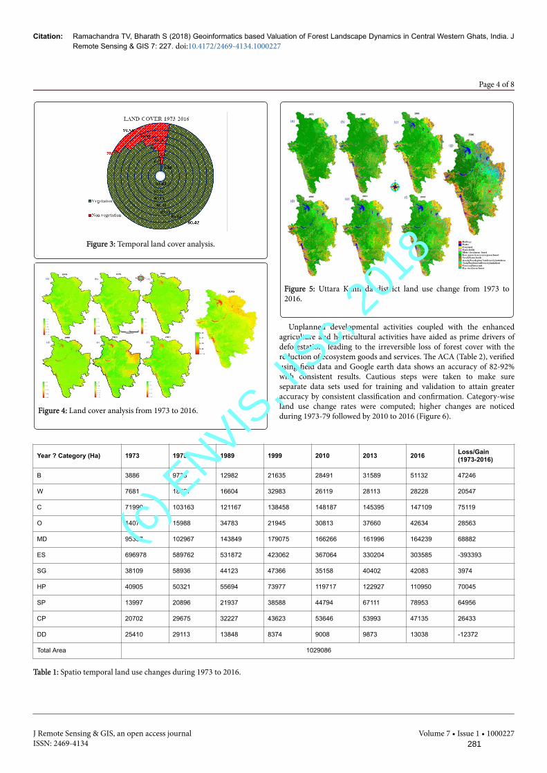
Figure 3: Temporal land cover analysis.
Figure 4: Land cover analysis from 1973 to 2016.
Figure 5: Uttara Kannada district land use change from 1973 to2016.
Unplanned developmental activities coupled with the enhancedagriculture and horticultural activities have aided as prime drivers ofdeforestation, leading to the irreversible loss of forest cover with thereduction of ecosystem goods and services. The ACA (Table 2), verifiedusing field data and Google earth data shows an accuracy of 82-92%with consistent results. Cautious steps were taken to make sureseparate data sets used for training and validation to attain greateraccuracy by consistent classification and confirmation. Category-wiseland use change rates were computed; higher changes are noticedduring 1973-79 followed by 2010 to 2016 (Figure 6).
Year ? Category (Ha) 1973 1979 1989 1999 2010 2013 2016 Loss/Gain(1973-2016)
B 3886 9738 12982 21635 28491 31589 51132 47246
W 7681 18527 16604 32983 26119 28113 28228 20547
C 71990 103163 121167 138458 148187 145395 147109 75119
O 14071 15988 34783 21945 30813 37660 42634 28563
MD 95357 102967 143849 179075 166266 161996 164239 68882
ES 696978 589762 531872 423062 367064 330204 303585 -393393
SG 38109 58936 44123 47366 35158 40402 42083 3974
HP 40905 50321 55694 73977 119717 122927 110950 70045
SP 13997 20896 21937 38588 44794 67111 78953 64956
CP 20702 29675 32227 43623 53646 53993 47135 26433
DD 25410 29113 13848 8374 9008 9873 13038 -12372
Total Area 1029086
Table 1: Spatio temporal land use changes during 1973 to 2016.
Citation: Ramachandra TV, Bharath S (2018) Geoinformatics based Valuation of Forest Landscape Dynamics in Central Western Ghats, India. JRemote Sensing & GIS 7: 227. doi:10.4172/2469-4134.1000227
Page 4 of 8
J Remote Sensing & GIS, an open access journalISSN: 2469-4134
Volume 7 • Issue 1 • 1000227281
(c) E
NVIS, I
ISc,
2018
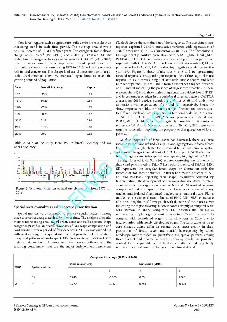
Non-forest regions such as agriculture, built environments show anincreasing trend in each time period. The built-up area shows apositive increase of 15.31% y-1(per year). The evergreen forest showschange of -2.78% y-1 (1973-1979) and -2.80% y-1 (2013-2016). Thegrater loss of evergreen forests can be seen as 3.53% y-1 (2010-2013)due to major motor ways expansion. Forest plantations andhorticulture show an increase during 1973 to 2016, indicating market’srole in land conversion. The abrupt land use changes are due to large-scale developmental activities, increased agriculture to meet thegrowing demand of population.
Year Overall Accuracy Kappa
1973 82.52 0.81
1979 84.29 0.81
1989 92.22 0.89
1999 90.71 0.87
2010 91.51 0.89
2013 91.98 0.90
2016 90.0 0.88
Table 2: ACA of the study. Here, PA Producer’s Accuracy and UAUser’s Accuracy.
Figure 6: Temporal variation of land use change rate from 1973 to2016.
Spatial metrics analysis and landscape prioritizationSpatial metrics were computed to quantify spatial patterns among
three diverse landscapes at class level over time. The analysis of spatialmetrics representing area, edge/border, compactness/dispersion, shapecategories provided an overall summary of landscape composition andconfiguration over a period of four decades. CATPCA was carried outwith relative weights of spatial metrics that provided vital insights tothe spatial patterns of landscape. CATPCA considering 1973 and 2016metrics data retained all components that were significant and theresulting components that are the major independent dimensions
(Table 3) shows the combination of the categories. The two dimensionstogether explained 74.49% cumulative variance with eigenvalues of7.98 (Dimension-1), 3.196 (Dimension-2) in 1973. The Dimension-1has significantly positive correlation with SHAPE_MN, FRAC_MN,PAFRAC, NLSI, CA representing shape complexity property andnegatively with CLUMPY, AI. The Dimension-2 represents NP, ED aspositive and AREA_MN, LPI are showing negative correlation for theyear 1973. Figure 7a shows taluks 1, 3, 4, 5, 9 and 10 representingforested regions (corresponding to major taluks of three agro-climaticregions) in 1973 form a single cluster with simple shapes and leastnumber of patches. Taluks 7 and 2 form a cluster with higher influenceof LPI and IJI indicating the presence of largest forest patches in theseregions. Sirsi (8) taluk show higher fragmentation evident from NP, EDand large number of edges in the peripheral forested patches. CATPCAanalysis for 2016 depicts cumulative variance of 69.14% under twodimensions with eigenvalues of 5.7 and 4.7 respectively. Figure 7bshows response variables exhibited a range of behaviours with respectto different levels of class proportion at temporal scale. In Dimension1, NP, LPI, ED, LSI, SHAPE_MN are positively correlated andPARA_MN, CLUMPY, AI are negatively correlated. Dimension-2represents CA, AREA_MN as positive and ENN_MN, NLSI representsnegative correlation depicting the property of disaggregation of forestpatches.
As class proportion of forest cover has decreased, there is a largeincrease in the standardized CLUMPY and aggregation indices, whichlead to form a single cluster for all coastal taluks with similar spatialpatterns of changes (coastal taluks 1, 2, 3, 4 and partly 5). The SahyadriInterior region show intra spatial heterogeneity highlighted by CA, IJI.The high forested taluk Supa (6) has not expressing any influence ofshape and patch metrics. Taluk 7 has major influence of SHAPE_MN,ED represents the irregular forest shape by alternation with theincrease of non-forest activities. Taluks 8 had major influence of NP,LSI and PAFRAC depicting their shape irregularity followed byfragmentation. The development of new individual non-forest patches,as reflected by the slightly increases in NP and LSI resulted in morecomplicated patch shapes in the meantime, also produced manysmaller and isolated fragmented patches at a temporal scale. Plains(taluks 10, 11) cluster shows influence of ENN_MN, NLSI as increaseof nearest neighbour of forest patch with decrease of mean area coverindicating the region is losing its forest cover abruptly at temporal scalewith increase in shape complexity. ED indicates that all taluksrepresenting simple edges (almost square) in 1973 and transform tocomplex with convoluted edges in all directions in 2016 due tofragmentation with newly developing edges. The landscapes of threeagro climatic zones differ in several ways, most clearly in theirproportion of forest cover and spatial heterogeneity by 2016.Landscape metrics aided in quantifying the spatial patterns amongthree distinct and diverse landscapes. This approach has providedcontext for interpretable set of landscape patterns that objectivelyrepresent temporal land use changes in each forested taluk.
Component loadings (1973 and 2016)
SNO Spatial metricsDimension (1973) Dimension (2016)
1 2 1 2
1 CA 0.649 -0.688 0.35 0.806
2 NP 0.370 0.743 0.786 -0.423
Citation: Ramachandra TV, Bharath S (2018) Geoinformatics based Valuation of Forest Landscape Dynamics in Central Western Ghats, India. JRemote Sensing & GIS 7: 227. doi:10.4172/2469-4134.1000227
Page 5 of 8
J Remote Sensing & GIS, an open access journalISSN: 2469-4134
Volume 7 • Issue 1 • 1000227282
(c) E
NVIS, I
ISc,
2018
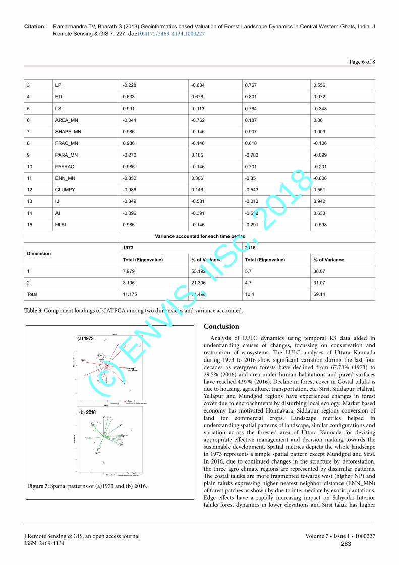
3 LPI -0.228 -0.634 0.767 0.556
4 ED 0.633 0.676 0.801 0.072
5 LSI 0.991 -0.113 0.764 -0.348
6 AREA_MN -0.044 -0.762 0.187 0.86
7 SHAPE_MN 0.986 -0.146 0.907 0.009
8 FRAC_MN 0.986 -0.146 0.618 -0.106
9 PARA_MN -0.272 0.165 -0.783 -0.099
10 PAFRAC 0.986 -0.146 0.701 -0.201
11 ENN_MN -0.352 0.306 -0.35 -0.806
12 CLUMPY -0.986 0.146 -0.543 0.551
13 IJI -0.349 -0.581 -0.013 0.942
14 AI -0.896 -0.391 -0.558 0.633
15 NLSI 0.986 -0.146 -0.291 -0.598
Variance accounted for each time period
Dimension1973 2016
Total (Eigenvalue) % of Variance Total (Eigenvalue) % of Variance
1 7.979 53.192 5.7 38.07
2 3.196 21.306 4.7 31.07
Total 11.175 74.498 10.4 69.14
Table 3: Component loadings of CATPCA among two dimensions and variance accounted.
Figure 7: Spatial patterns of (a)1973 and (b) 2016.
ConclusionAnalysis of LULC dynamics using temporal RS data aided in
understanding causes of changes, focussing on conservation andrestoration of ecosystems. The LULC analyses of Uttara Kannadaduring 1973 to 2016 show significant variation during the last fourdecades as evergreen forests have declined from 67.73% (1973) to29.5% (2016) and area under human habitations and paved surfaceshave reached 4.97% (2016). Decline in forest cover in Costal taluks isdue to housing, agriculture, transportation, etc. Sirsi, Siddapur, Haliyal,Yellapur and Mundgod regions have experienced changes in forestcover due to encroachments by disturbing local ecology. Market basedeconomy has motivated Honnavara, Siddapur regions conversion ofland for commercial crops. Landscape metrics helped inunderstanding spatial patterns of landscape, similar configurations andvariation across the forested area of Uttara Kannada for devisingappropriate effective management and decision making towards thesustainable development. Spatial metrics depicts the whole landscapein 1973 represents a simple spatial pattern except Mundgod and Sirsi.In 2016, due to continued changes in the structure by deforestation,the three agro climate regions are represented by dissimilar patterns.The costal taluks are more fragmented towards west (higher NP) andplain taluks expressing higher nearest neighbor distance (ENN_MN)of forest patches as shown by due to intermediate by exotic plantations.Edge effects have a rapidly increasing impact on Sahyadri Interiortaluks forest dynamics in lower elevations and Sirsi taluk has higher
Citation: Ramachandra TV, Bharath S (2018) Geoinformatics based Valuation of Forest Landscape Dynamics in Central Western Ghats, India. JRemote Sensing & GIS 7: 227. doi:10.4172/2469-4134.1000227
Page 6 of 8
J Remote Sensing & GIS, an open access journalISSN: 2469-4134
Volume 7 • Issue 1 • 1000227283
(c) E
NVIS, I
ISc,
2018
NP due to more intermediate patches of non-forest types. CATPCAalong with spatial metric clustering information visually demonstratedthe ability of these metrics to express the variation of patterns at thelandscape scale. Variation in landscape spatial heterogeneity/similarityhas provided regional level picture of the district, which can be used toframe conservation policies to protect social and ecologicalsustainability of ecosystems.
AcknowledgementsWe acknowledge the sustained financial support for ecological
research in Western Ghats from (i) NRDMS division, The Ministry ofScience and Technology (DST), Government of India, (ii) Indianinstitute of Science and (iii) ENVIS division, The Ministry ofEnvironments, Forests and Climate Change, Government of India. Wethank Vishnu Mukri and Srikanth Naik for the assistance during fielddata collection.
References1. Forman RTT, Godron M (1986) Landscape Ecology. Willey, New York,
USA.2. Lambin EF, Geist H, Lepers E (2003) Dynamics of land use and land
cover change in tropical regions. Environment and Resources 28:205-241.
3. Ramachandra TV, Bharath S, Bharath HA (2012) Peri-Urban to UrbanLandscape Patterns Elucidation through Spatial Metrics. InternationalJournal of Engineering Research and Development 2: 58-81.
4. Ramachandra TV, Bharath S, Nimish G (2018) Modelling landscapedynamics with LST in protected areas of Western Ghats,Karnataka. Journal of Environmental Management 206: 1253-1262.
5. Dupont L, Van EV (2013) Assessing the potential impacts of climatechange on traditional landscapes and their heritage values on the locallevel: Case studies in the Dender basin in Flanders, Belgium. Land UsePolicy 35: 179-191.
6. Bharath S, Rajan KS, Ramachandra TV (2013) Land Surface TemperatureResponses to Land Use Land Cover Dynamics. Geoinfor Geostat AnOverview 1: 4.
7. Ramachandra TV, Shruthi BV (2007) Spatial mapping of renewableenergy potential. Renewable and Sustainable Energy Reviews 11:1460-1480.
8. Kindu M, Schneider T, Teketay D, Knoke T (2016) Changes of ecosystemservice values in response to land use/land cover dynamics in Munessa–Shashemene landscape of the Ethiopian highlands. Science of the TotalEnvironment 547: 137-147.
9. Bharath S, Nimish G, Ramachandra TV (2017) Visualization andPrediction of Landscape Dynamics in The Protected Areas of Karnataka.International Journal of Research in Engineering and Technology 6:53-62.
10. Simon B, Che E, Robert H, Adrienne G (2012) Assessing the impacts ofeconomic and climate changes on land-use in mountain regions: A spatialdynamic modeling approach. Agriculture Ecosystems & Environment149: 50-63.
11. Geneletti D (2015) A conceptual approach to promote the integration ofecosystem services in strategic environmental assessment. Journal ofEnvironmental Assessment Policy and Management 17: 1-27.
12. Smiraglia D, Ceccarelli T, Bajocco S, Salvati L, Perini L (2016) Linkingtrajectories of land change, land degradation processes and ecosystemservices. Environmental Research 147: 590-600.
13. Vinay S, Bharath S, Bharath HA, Ramachandra TV (2013) Hydrologicmodel with landscape dynamics for drought monitoring. Proceeding ofJoint International Workshop of ISPRS WG VIII/1 and WG IV/4 onGeospatial Data for Disaster and Risk Reduction, Hyderabad, India, pp:21-22.
14. Zhou W, Troy A, Grove M (2008) Modeling residential lawn fertilizationpractices: Integrating high resolution remote sensing with socioeconomicdata. Environmental Management 41: 742-752.
15. Svoray T, Avi P, Atkinson PM (2013) Ecological sustainability inrangelands: the contribution of remote sensing. International Journal ofRemote Sensing 34: 6216-6242.
16. McGarigal K, Marks BJ (1995) FRAGSTATS: Spatial pattern analysisprogram for quantifying landscape structure. Gen Tech Report PNW-GTR-351, USDA Forest Service, Pacific Northwest Research Station,Portland, Oregon, USA.
17. Herold M, Couclelis H, Clarke KC (2005) The role of spatial metrics inthe analysis and modeling of urban land use change. Computers,Environment and Urban Systems 29: 369-399.
18. Uuemaa E, Antrop M, Roosaare J, Marja R, Mander U (2009) LandscapeMetrics and Indices: An Overview of Their Use in Landscape Research.Living Reviews in Landscape Research 3: 1-28.
19. Bhattarai K, Conway D, Mahmoud Y (2009) Determinants ofdeforestation in Nepal's central development region. Journal ofEnvironmental Management 91: 471-488.
20. Jiao L, Liu Y, Li H (2012) Characterizing land-use classes in remotesensing imagery by shape metrics. ISPRS Journal of Photogrammetry andRemote Sensing 72: 46-55.
21. Ramachandra TV, Bharath S, Bharath AH (2014) Spatio-temporaldynamics along the terrain gradient of diverse landscape. Journal ofEnvironmental Engineering and Landscape Management 22: 50-63.
22. Jackson DA (1993) Stopping rules in principal components analysis: acomparison of heuristical and statistical approaches. Ecology 74:2204-2214.
23. Samuel AC, McGarigal K, Neel MC (2008) Parsimony in landscapemetrics: Strength, universality, and consistency. Ecological Indicators 8:691-703.
24. Meulman JJ, Heiser WJ (2004) SPPS, SPSS Categories 13.0. Chicago,USA.
25. Linting M, Meulman JJ, Groenen PJ, van der Koojj AJ (2007) Nonlinearprincipal components analysis: introduction and application.Psychological methods 12: 336-358.
26. Pascal JP (1986) Explanatory booklet on the forest map of South India.French Institute, Pondicherry, India 3: 19-30.
27. Nelson RF (1983) Detecting forest canopy change due to insect activityusing Landsat MSS. Photogrammetric Engineering & Remote Sensing 49:1303-1314.
28. Lillesand T, Kiefer RW, Chipman J (2014) Remote sensing and imageinterpretation. John Wiley & Sons, New Jersey, USA.
29. Kennedy RE, Townsend PA, Gross JE, Cohen WB, Bolstad P, et al. (2009)Remote sensing change detection tools for natural resource managers:understanding concepts and tradeoffs in the design of landscapemonitoring projects. Remote Sensing of Environment 113: 1382-1396.
30. Liu C, Frazier P, Kumar L (2007) Comparative assessment of themeasures of thematic classification accuracy. Remote Sensing ofEnvironment 107: 606-616.
31. FAO (1995) Forest resources assessment 1990: Global Synthesis. Rome.32. Puyravaud JP (2003) Standardizing the evaluation of the annual rate of
deforestation. Forest Ecology Management 177: 593-596.33. Armenteras D, Rudas G, Rodriguez N, Sua S, Romero M (2006) Patterns
and causes of deforestation in the Colombian Amazon. EcologicalIndicators 6: 353-368.
34. Riitters KH, O'Neill RV, Hunsaker CT, Wickham JD, Yankee DH, et al.(1995) A factor analysis of landscape pattern and structure metrics.Landscape Ecology 10: 23-39.
35. Echeverria C, David AC, Hall M, Newton AC (2008) Spatially explicitmodels to analyze forest loss and fragmentation between 1976 and 2020in southern Chile. Ecological Modelling 212: 439-449.
36. Tabor K, Burgess ND, Mbilinyi BP, Kashaigili JJ, Steininger MK (2010)Forest and woodland cover and change in coastal Tanzania and Kenya,1990 to 2000. Journal of East African Natural History 99: 19-45.
Citation: Ramachandra TV, Bharath S (2018) Geoinformatics based Valuation of Forest Landscape Dynamics in Central Western Ghats, India. JRemote Sensing & GIS 7: 227. doi:10.4172/2469-4134.1000227
Page 7 of 8
J Remote Sensing & GIS, an open access journalISSN: 2469-4134
Volume 7 • Issue 1 • 1000227284
(c) E
NVIS, I
ISc,
2018

37. Setturu B, Bharath HA, Sanna Durgappa D, Ramachandra TV (2012)Landscape dynamics through spatial metrics. Proceedings of IndiaGeoSpatial Conference, Epicentre, Gurgaon, India.
38. Plexida SG, Sfougaris AI, Ispikoudis IP, Papanastasis VP (2014) Selectinglandscape metrics as indicators of spatial heterogeneity—A comparisonamong Greek landscapes. International Journal of Applied EarthObservation and Geoinformation 26: 26-35.
39. Singh SK, Srivastava PK, Szabó S, Petropoulos GP, Gupta M, et al. (2017)Landscape transform and spatial metrics for mapping spatiotemporalland cover dynamics using Earth Observation data-sets. GeocartoInternational 32: 113-27.
40. Turner MG, Simard M (2017) Using Spatial Statistics and LandscapeMetrics to Compare Disturbance Mosaics. In: Learning LandscapeEcology. Springer, New York, USA, pp: 175-190.
Citation: Ramachandra TV, Bharath S (2018) Geoinformatics based Valuation of Forest Landscape Dynamics in Central Western Ghats, India. JRemote Sensing & GIS 7: 227. doi:10.4172/2469-4134.1000227
Page 8 of 8
J Remote Sensing & GIS, an open access journalISSN: 2469-4134
Volume 7 • Issue 1 • 1000227285
(c) E
NVIS, I
ISc,
2018
Green Skill Development Programme, MOEFCC, GoI– GSDP Manual
ENVIS Resource Partner: Sahyadri ENVIS, CES, IISc, Bengaluru;
ENVIS Hub: EMPRI, Bengaluru.
ENERGY AND WETLANDS RESEARCH GROUP
CENTRE FOR ECOLOGICAL SCIENCES
NEW BIOSCIENCE BUILDING, III FLOOR, E-WING, LAB: TE15
Indian Institute of Science, Telephone: 91-80-
22933099/22933503(Ext:107)/23600985
Fax: 91-80-23601428/23600085/23600683[CES-TVR]
Email: [email protected]; envis.ces@ iisc.ac.in
Web: http://ces.iisc.ernet.in/energy, http://ces.iisc.ernet.in/biodiversity
Open Source GIS: http://ces.iisc.ernet.in/grass
Related Documents