58 American Economic Journal: Economic Policy 2012, 4(1): 58–97 http://dx.doi.org/10.1257/pol.4.1.58 E xposure to airborne pollution has substantial adverse health consequences. 1 A recent World Health Organization (WHO) study has estimated that urban air pollution accounts for 6.4 million years of life lost worldwide annually (Cohen et al. 2004). Many harmful pollutants are emitted by automobiles. For example, Currie and Walker (2011) estimate that prenatal exposure to traffic congestion alone reduces welfare in the United States by $557 million per year. However, while the adverse health consequences of automobile pollution are widely acknowledged, little is known about the effects of transportation infrastructure on air pollution. In this paper, we ask whether the air quality effects of one major type of transportation infrastructure—urban rail transit—represent significant benefits. Conceptually, whether rail transit infrastructure has any meaningful effects on air quality is unclear. On the one hand, a rich theoretical literature following Mohring (1972) has argued that rail transit is subject to increasing returns to scale. Ridership increases engender higher service frequencies, reduce the average waiting times at stops, thus encouraging further ridership. The “Mohring Effect” implies that invest- ments in rail transit infrastructure divert marginal automobile travelers away from 1 For recent examples, see Currie and Neidell (2005) and Chay and Greenstone (2003) for evidence on the infant mortality effects of exposure to air pollution. * Chen: School of Social Sciences, Humanities and Arts, University of California - Merced, 5200 N. Lake Road, Merced, CA 95343 (e-mail: [email protected]); Whalley: School of Social Sciences, Humanities and Arts, University of California - Merced, 5200 N. Lake Road, Merced, CA 95343 and National Bureau of Economic Research, 1050 Massachusetts Avenue, Cambridge, MA 02138 (e-mail: [email protected]). We thank Severin Borenstein, Lucas Davis, Rob Innes, Mark Jacobsen, Shawn Kantor, Catherine Wolfram, anonymous referees, and participants at the 11th Occasional California Workshop on Environmental and Natural Resource Economics at UC Santa Barbara, and seminars at UC Berkeley and UC Merced for helpful comments. We are grate- ful to the excellent research assistance provided by Chi-Chung Tsao. All errors are our own. † To comment on this article in the online discussion forum, or to view additional materials, visit the article page at http://dx.doi.org/10.1257/pol.4.1.58. Green Infrastructure: The Effects of Urban Rail Transit on Air Quality † By Yihsu Chen and Alexander Whalley* The transportation sector is a major source of air pollution world- wide, yet little is known about the effects of transportation infrastruc- ture on air quality. This paper quantifies the effects of one major type of transportation infrastructure—urban rail transit—on air quality using the sharp discontinuity in ridership on opening day of a new rail transit system in Taipei. We find that the opening of the Metro reduced air pollution from one key tailpipe pollutant, carbon monox- ide, by 5 to 15 percent. Little evidence that the opening of the Metro affected ground level ozone pollution is found however. (JEL L92, Q53, R41, R53)

Welcome message from author
This document is posted to help you gain knowledge. Please leave a comment to let me know what you think about it! Share it to your friends and learn new things together.
Transcript
58
American Economic Journal: Economic Policy 2012, 4(1): 58–97http://dx.doi.org/10.1257/pol.4.1.58
Exposure to airborne pollution has substantial adverse health consequences.1 A recent World Health Organization (WHO) study has estimated that urban
air pollution accounts for 6.4 million years of life lost worldwide annually (Cohen et al. 2004). Many harmful pollutants are emitted by automobiles. For example, Currie and Walker (2011) estimate that prenatal exposure to traffic congestion alone reduces welfare in the United States by $557 million per year. However, while the adverse health consequences of automobile pollution are widely acknowledged, little is known about the effects of transportation infrastructure on air pollution. In this paper, we ask whether the air quality effects of one major type of transportation infrastructure—urban rail transit—represent significant benefits.
Conceptually, whether rail transit infrastructure has any meaningful effects on air quality is unclear. On the one hand, a rich theoretical literature following Mohring (1972) has argued that rail transit is subject to increasing returns to scale. Ridership increases engender higher service frequencies, reduce the average waiting times at stops, thus encouraging further ridership. The “Mohring Effect” implies that invest-ments in rail transit infrastructure divert marginal automobile travelers away from
1 For recent examples, see Currie and Neidell (2005) and Chay and Greenstone (2003) for evidence on the infant mortality effects of exposure to air pollution.
* Chen: School of Social Sciences, Humanities and Arts, University of California - Merced, 5200 N. Lake Road, Merced, CA 95343 (e-mail: [email protected]); Whalley: School of Social Sciences, Humanities and Arts, University of California - Merced, 5200 N. Lake Road, Merced, CA 95343 and National Bureau of Economic Research, 1050 Massachusetts Avenue, Cambridge, MA 02138 (e-mail: [email protected]). We thank Severin Borenstein, Lucas Davis, Rob Innes, Mark Jacobsen, Shawn Kantor, Catherine Wolfram, anonymous referees, and participants at the 11th Occasional California Workshop on Environmental and Natural Resource Economics at UC Santa Barbara, and seminars at UC Berkeley and UC Merced for helpful comments. We are grate-ful to the excellent research assistance provided by Chi-Chung Tsao. All errors are our own.
† To comment on this article in the online discussion forum, or to view additional materials, visit the article page at http://dx.doi.org/10.1257/pol.4.1.58.
Green Infrastructure: The Effects of Urban Rail Transit on Air Quality†
By Yihsu Chen and Alexander Whalley*
The transportation sector is a major source of air pollution world-wide, yet little is known about the effects of transportation infrastruc-ture on air quality. This paper quantifies the effects of one major type of transportation infrastructure—urban rail transit—on air quality using the sharp discontinuity in ridership on opening day of a new rail transit system in Taipei. We find that the opening of the Metro reduced air pollution from one key tailpipe pollutant, carbon monox-ide, by 5 to 15 percent. Little evidence that the opening of the Metro affected ground level ozone pollution is found however. (JEL L92, Q53, R41, R53)
ContentsGreen Infrastructure: The Effects of Urban Rail Transit on Air Quality† 58
I. Institutional Setting and Empirical Approach 62A. Institutional Setting 62B. Empirical Approach 65II. Data 70III. Results 74A. OLS Results 74B. Main Results: Two-Year Window Specification 74C. Identifying Assumption Validity and Robustness Checks: Two-Year Window Specification 75D. Main Results: 30-Day Window Specification 82E. Estimate Magnitudes 88F. Heterogeneous Effects 91IV. Conclusion 94References 95
VoL. 4 No. 1 59CHEN ANd WHALLEy: GrEEN INfrAsTruCTurE
their vehicles resulting in a traffic diversion effect, and thereby reduce air pollution. On the other hand, another highly influential literature following Vickrey(1969) argues that investments in transportation infrastructure simply induce demand for travel, resulting in a traffic creation effect. As rail transit infrastructure investments are likely to both divert travelers away from automobile travel, as well as induce more travel, the net effect on automobile travel—and air pollution—is unclear.
Beyond an obvious interest for transportation and environmental economists, the question of whether rail transit infrastructure has meaningful air quality effects has tre-mendous practical relevance. Every day 155 million people travel on urban rail transit systems in over 110 cities throughout the world and publicly subsidized investments in rail transit infrastructure continue to grow (International Association of Public Transport 2009). Since the year 2000 alone, urban rail transit systems in 37 cities have opened, including Delhi, Dubai, and most recently Shenyang, China. Indeed, rail transit advocates and policy makers often point to the environmental benefits of rail transit infrastructure to justify these substantial investments. For example, an initiative to transform Beijing into a “public transport city” by doubling the size of the metro system from 224 km to 554 km of track by 2015 is based on the goal of reducing air pollution below 2008 levels (CCTV 2009). Similarly, in the United States, the Obama administration recently announced that the environmental effects of rail transit will be taken into account in the allocation of federal funding (Cooper 2010).
While environmental impacts often feature prominently in transportation policy debates, traditional estimates of the benefits of transportation infrastructure have focused largely on the value of reduced travel time.2 More recently the literature has used two approaches to incorporate a broader set of effects in cost-benefit estimates.3 A first approach uses a hedonic method based on differences in house prices in neigh-borhoods with and without access to rail transit to value rail transit infrastructure.4 A recent example of this approach is Gibbons and Machin (2005) who study the effects of the expansion of the London Underground system and find a 7 to 20 percent shift in house prices for a one-standard-deviation reduction in distance to the rail transit. However, as the air quality effects of rail transit infrastructure are likely to be citywide, neighborhood comparisons may not fully capture the air quality effects.
A second approach uses the best available estimates of the many potential effects of rail transit in a highly complete model and computes optimal rail transit subsidies.5
2 Seminal contributions on the effects of transportation infrastructure include Fernald (1999). For a few recent examples see papers such as Baum-Snow and Kahn (2005) on modes of travel, Baum-Snow (2007) on suburbaniza-tion, and Michaels (2008) on trade. See Small and Verhoef (2007) for an excellent overview of the economics of urban transportation. See Mackie et al. (2001) and also Small and Verhoef (2007) for discussions of the traditional approach.
3 While the literature on transportation infrastructure has generally not discussed environmental effects, there is now a substantial literature on automobile externalities and policies that incorporates environmental effects. Recent studies examining taxation of automobile travel include Feng, Fullerton, and Gan (2005) and Fullerton and Gan (2005) who study whether second-best taxes on automobile travel can be similarly effective as a first-best tax. Similarly, Parry and Small (2005) study optimal gas taxes and find that gas taxes in the United States are lower than the optimal gas tax, but higher in the UK. Davis (2008) demonstrates that regulations designed to reduce vehicle travel in Mexico City have virtually no effect on air quality. Similarly, Auffhammer and Kellogg (2009) show that gasoline content regulations are largely ineffective in reducing ground-level ozone pollution in the United States. See Parry, Walls, and Harrington (2007) for a survey of automobile externalities and policies.
4 See Gibbons and Machin (2008) for a survey of the literature that uses the hedonic method to value transporta-tion infrastructure.
5 See Parry and Small (2009) for a survey of the literature that computes optimal transit subsidies.
60 AMErICAN ECoNoMIC JourNAL: ECoNoMIC PoLICy fEBruAry 2012
A recent example is Parry and Small (2009) who incorporate the costs of air pollution, among numerous other factors. They find that even starting with fares at 50 percent of operating costs, incremental fare reductions are welfare improving in almost all cases. Conclusions about the importance of air quality effects hinge crucially on the esti-mated behavioral responses and social costs of automobile travel incorporated into the models. As many key parameter estimates are subject to debate, whether this approach fully captures the air quality effects remains an open question.
The central empirical challenge in measuring the effects of rail transit infrastruc-ture on air quality is one of identification. Variation in rail transit infrastructure that is not confounded with other factors, that also affect air pollution, is difficult to come by. For example, rail transit infrastructure is likely to be built in areas where the demand for automobile travel, and hence air pollution, is likely to be elevated anyway. Variation in the utilization of a particular rail transit system over time is similarly problematic. Times of the day when the utilization of rail transit infrastruc-ture is especially high are also likely to be times when automobile travel, and air pollution are similarly elevated. Credible estimates of the air quality effects of rail transit infrastructure require a solution to the identification problem.
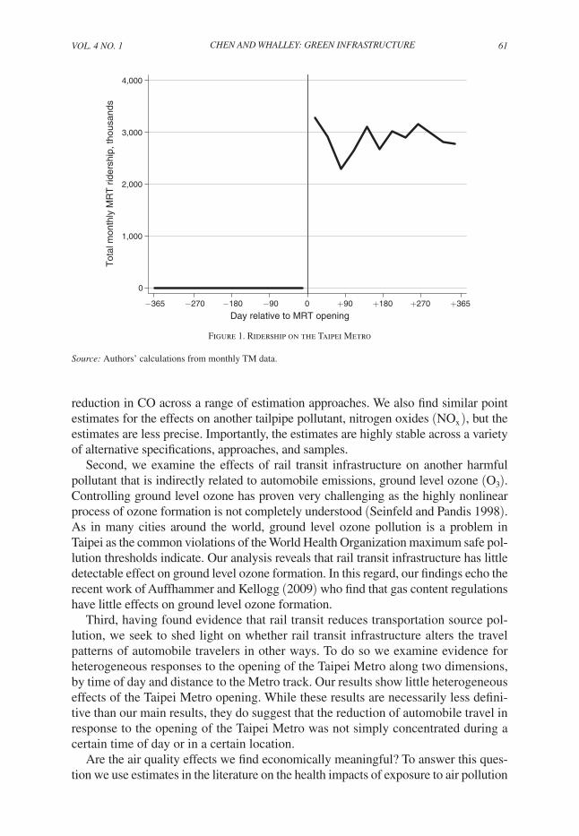
In this paper we tackle the identification challenge by exploiting exogenous varia-tion in the availability of rail transit infrastructure from the opening of a new metro system in Taipei, Taiwan. We use the discontinuity in rail transit ridership on opening day of the Taipei Metro system to identify the effect of rail transit infrastructure on air pollution based on a discontinuity based (DB) approach. Because high frequency air pollution data for a range of pollutants were collected before and after the opening date of the Metro system, Taipei provides a uniquely compelling context to estimate these effects. Figure 1 displays the time series of Taipei Metro ridership and clearly shows the sharp discontinuity in ridership on opening day (March 28, 1996). It is this discontinuity in rail transit availability that forms the heart of our analysis.6
The identifying assumption underlying our ridership discontinuity approach is that in the absence of opening the Taipei Metro, air quality would have changed smoothly on March 28, 1996, in Taipei. More precisely, air pollution levels in Taipei on the days just before the opening of the Taipei Metro form a valid counterfactual for air pollu-tion levels in Taipei on days just after the opening of the Taipei Metro, conditional on differences in weather, a host of time-specific fixed effects, and a very flexible smooth time trend. This assumption seems reasonable as construction delays and safety issues are highly uncertain, and Metro operators would have faced great difficulties in holding back the opening of the Taipei Metro from an expectant public for any strategic reasons.
Our analysis reveals three main findings. First, we find significant effects for trans-portation source air pollution. Our ridership discontinuity based analysis indicates that the opening of the Taipei Metro caused a meaningful reduction in the concentration of one tailpipe pollutant, carbon monoxide (CO). The effects appear to be both statisti-cally and economically significant as the Taipei Metro opening caused a 5 to 15 percent
6 Our approach is similar in spirit to recent studies in the public health literature on the impact of transportation restrictions imposed during the Olympics on air quality and health outcomes. Examples include Friedman et al. (2001) who examine the effect of the 1996 Olympics in Atlanta on air quality and asthma, and Li et al. (2010) who examine the effect of the 2008 Olympics in Beijing on asthma.
VoL. 4 No. 1 61CHEN ANd WHALLEy: GrEEN INfrAsTruCTurE
reduction in CO across a range of estimation approaches. We also find similar point estimates for the effects on another tailpipe pollutant, nitrogen oxides ( NO x ), but the estimates are less precise. Importantly, the estimates are highly stable across a variety of alternative specifications, approaches, and samples.
Second, we examine the effects of rail transit infrastructure on another harmful pollutant that is indirectly related to automobile emissions, ground level ozone ( O 3 ). Controlling ground level ozone has proven very challenging as the highly nonlinear process of ozone formation is not completely understood (Seinfeld and Pandis 1998). As in many cities around the world, ground level ozone pollution is a problem in Taipei as the common violations of the World Health Organization maximum safe pol-lution thresholds indicate. Our analysis reveals that rail transit infrastructure has little detectable effect on ground level ozone formation. In this regard, our findings echo the recent work of Auffhammer and Kellogg (2009) who find that gas content regulations have little effects on ground level ozone formation.
Third, having found evidence that rail transit reduces transportation source pol-lution, we seek to shed light on whether rail transit infrastructure alters the travel patterns of automobile travelers in other ways. To do so we examine evidence for heterogeneous responses to the opening of the Taipei Metro along two dimensions, by time of day and distance to the Metro track. Our results show little heterogeneous effects of the Taipei Metro opening. While these results are necessarily less defini-tive than our main results, they do suggest that the reduction of automobile travel in response to the opening of the Taipei Metro was not simply concentrated during a certain time of day or in a certain location.
Are the air quality effects we find economically meaningful? To answer this ques-tion we use estimates in the literature on the health impacts of exposure to air pollution
Figure 1. Ridership on the Taipei Metro
source: Authors’ calculations from monthly TM data.
0
1,000
2,000
3,000
4,000
Tot
al m
onth
ly M
RT
rid
ersh
ip, t
hous
ands
−365 −270 −180 −90 0 +90 +180 +270 +365
Day relative to MRT opening
62 AMErICAN ECoNoMIC JourNAL: ECoNoMIC PoLICy fEBruAry 2012
to understand the health effects that our results would imply. The benefits of the implied health effects are significantly larger than those incorporated in prior work. Strikingly, our estimates are more than double those incorporated into the Parry and Small (2009) optimal rail transit subsidy calculations. Furthermore, the fact that our estimates account for at least 30 percent of the social value of rail transit infrastructure estimated by Parry and Small (2009) indicates that the air quality benefits we measure are a substantial component of the benefit of rail transit infrastructure.7
The availability of air pollution data from other sources and other cities in Taiwan provides a number of opportunities to evaluate the credibility of our identification strategy. We first examine whether other air pollutants closely related to indus-try activity (and presumably the demand for travel) also display a discontinuous change in Taipei on the day that the Taipei Metro opened. Comfortingly, we find little evidence that the Taipei Metro was opened on a day when local demand for travel appeared to be especially high or low. Second, we examine whether the same transportation source pollutants in two other Taiwanese air sheds (Kaohsiung and the east coast) also display a discontinuity on the day the Metro system opened in Taipei. Again we find little evidence that the Taipei Metro was opened on a day when automobile pollution was especially high or low in Taiwan. Lastly, we use the air pollution outcomes in Kaohsiung in the narrow window around the Taipei Metro opening date as a control to conduct a simple difference-in-differences analysis that also yields very similar conclusions. These tests and alternative approach estimates provide further support for the validity of our main findings.
The remainder of the paper is organized as follows. Section I provides the insti-tutional setting and outlines the empirical approach. Section II describes the data. Section III presents the results. Section IV concludes.
I. Institutional Setting and Empirical Approach
A. Institutional setting
Simple comparisons suggest that Taipei is most comparable to highly dense cities in the emerging economies of East Asia. The metropolitan Taipei area is located in the Taipei Basin in northern Taiwan, stretching over approximately 900 square miles. In 2009, the total population was 2.7 million in Taipei city, with nearly 6.5 million in the greater metro area. The country’s per capita income was US $15,000 in 2009, compatible with other countries such as South Korea and about one-third that of the United States (International Monetary Fund 2009). The Taipei metropolitan area is highly populated with a density of approximately 25,000 people per square mile, roughly comparable to New York City.
The public transportation system in Taipei has improved substantially since the Taipei Metro system began operating in 1996. The planning and construction of
7 Environmental effects are frequently included in the Environmental Impact Assessments (EIAs) required in many local planning processes. However, as the environmental effects incorporated in EIAs are often vague, dif-ficult to verify, and subject to influence by interest groups (Dipper 1998) economists have typically sought other methods to quantify the costs and benefits of transportation infrastructure.
VoL. 4 No. 1 63CHEN ANd WHALLEy: GrEEN INfrAsTruCTurE
the Metro was a lengthy and highly uncertain process that involved the displace-ment of various communities, numerous protests, and wrestling among compet-ing interest groups. The original concept for the Metro was initiated in 1967 in anticipation of the increasing traffic congestion and resulting air pollution prob-lems expected in a rapidly growing economy. However, it was not until 20 years later that the master plan specifying the routes, transportation capacity, and other engineering details was completed. The official construction began in December 1988. The first line was opened on March 28, 1996. Importantly for the empirical analysis, the planning and announcement of the precise route occurred many years in advance of the actual opening day, allowing time for households and firms to undertake substantial adjustments.
After construction began, the initial opening day of the Taipei Metro was sched-uled to be on December 31, 1992. However, opening day was soon postponed to August 12, 1993 as delays in construction as well as difficulties in integrating com-munication and operation systems lead to slow progress. The project also expe-rienced further setbacks. For example, during an operating test on May 5, 1993, one train caught fire due to the overheating of the brake system upon attempting to enter a station. A similar accident resulting in trains being derailed and burned occurred on September 24, 1993 due to a malfunction of the automatic-control system. As the numerous safety issues had become apparent government regula-tors took an even larger role in determining when the metro was safe to operate. Ultimately, the Taipei Metro was not fully inspected and certified by the govern-ment until May 5, 1995. The opening date of Taipei Metro was finally set to be March 28, 1996 after a successful public test ride on February 27, 1996.
There were of course other public transport alternatives to a metro system avail-able in Taipei. One prominent alternative was high speed buses. As a number of authors have argued that high speed buses are more likely to pass the cost-benefit test than a subway system (see for example Kain 1992, and Gordon and Kolesar 2011) it is worthwhile to discuss the decision to invest in a metro system in Taipei. One key reason was the international rivalry with mainland China. The fact that Beijing was due to open a subway system in 1971 led to public pressure to plan a similar system in Taipei, which opened long after it was initially planned. The international rivalry rationale for the Metro is reflected in how the project was funded. The central Taiwanese government contributed two-thirds of the costs, and the city government contributed only one third of the total costs. A second reason for the construction of a subway rather than utilizing high speed busses was the lack of a road network in Taipei capable of handling high speed busses. The pre-metro road network consisted of many narrow short streets that frequently turned at sharp angles due to a poorly organized city planning process. To imple-ment a meaningful high speed bus system an entirely new network of high speed roads would first have to be constructed. Thus, it seems that the decision to con-struct the Taipei Metro rather then invest in high speed buses was primarily driven by international rivalry and a lack of a road network capable of handling high speed busses rather than air pollution concerns.
As shown in Figure 2, the original Taipei Metro system began with a single route. The dotted line in the figure indicates the first route, Muzha, that was opened on
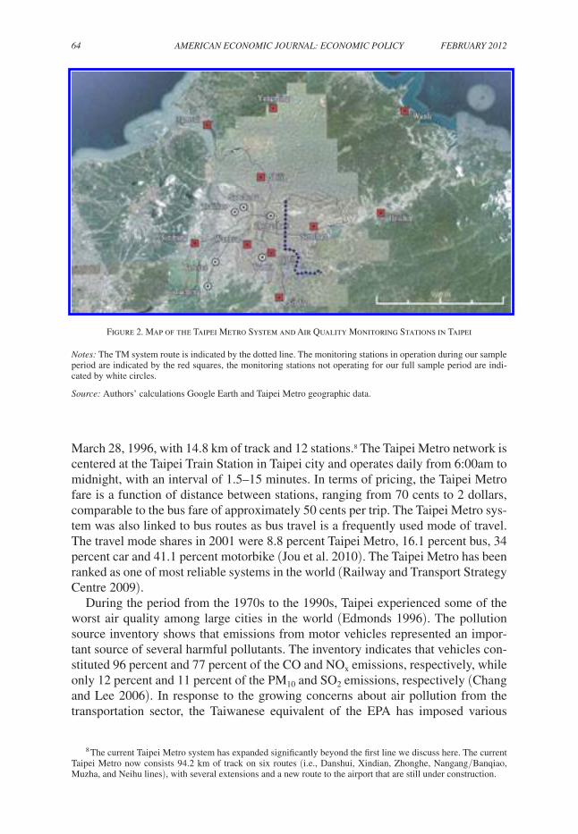
64 AMErICAN ECoNoMIC JourNAL: ECoNoMIC PoLICy fEBruAry 2012
March 28, 1996, with 14.8 km of track and 12 stations.8 The Taipei Metro network is centered at the Taipei Train Station in Taipei city and operates daily from 6:00am to midnight, with an interval of 1.5–15 minutes. In terms of pricing, the Taipei Metro fare is a function of distance between stations, ranging from 70 cents to 2 dollars, comparable to the bus fare of approximately 50 cents per trip. The Taipei Metro sys-tem was also linked to bus routes as bus travel is a frequently used mode of travel. The travel mode shares in 2001 were 8.8 percent Taipei Metro, 16.1 percent bus, 34 percent car and 41.1 percent motorbike (Jou et al. 2010). The Taipei Metro has been ranked as one of most reliable systems in the world (Railway and Transport Strategy Centre 2009).
During the period from the 1970s to the 1990s, Taipei experienced some of the worst air quality among large cities in the world (Edmonds 1996). The pollution source inventory shows that emissions from motor vehicles represented an impor-tant source of several harmful pollutants. The inventory indicates that vehicles con-stituted 96 percent and 77 percent of the CO and N O x emissions, respectively, while only 12 percent and 11 percent of the P M 10 and S O 2 emissions, respectively (Chang and Lee 2006). In response to the growing concerns about air pollution from the transportation sector, the Taiwanese equivalent of the EPA has imposed various
8 The current Taipei Metro system has expanded significantly beyond the first line we discuss here. The current Taipei Metro now consists 94.2 km of track on six routes (i.e., Danshui, Xindian, Zhonghe, Nangang/Banqiao, Muzha, and Neihu lines), with several extensions and a new route to the airport that are still under construction.
Figure 2. Map of the Taipei Metro System and Air Quality Monitoring Stations in Taipei
Notes: The TM system route is indicated by the dotted line. The monitoring stations in operation during our sample period are indicated by the red squares, the monitoring stations not operating for our full sample period are indi-cated by white circles.
source: Authors’ calculations Google Earth and Taipei Metro geographic data.
VoL. 4 No. 1 65CHEN ANd WHALLEy: GrEEN INfrAsTruCTurE
regulations over the years. These include performance standards that impose limits on tailpipe emissions of CO and N O x for newly manufactured vehicles and scooters. In compliance with the standards, manufactures have enhanced vehicle and scooter performance by introducing more efficient fuel injection, carburetors systems, or catalytic convertors. At the same time, reformulated gasoline (RFG) regulations have been introduced to reduce sulfur content in gasoline and diesel in 1992, 1995, and 1997.9 In addition, tax revenue from fuel consumption has been used to fund various programs related to air quality, including vehicle inspection and mainte-nance, subsides for retrofitting particulate filters, etc. (Taiwanese EPA 2009a). One of the key challenges for the empirical analysis is to separate the effects of the Taipei Metro from these other environmental and transportation policy changes that also effect air pollution.
B. Empirical Approach
In this section we introduce the empirical approaches we use. We first describe a basic Ordinary Least Squares (OLS) approach to estimate the conditional correla-tion between transit ridership and air pollution in Taipei over time. The OLS models serve as a useful baseline for our main estimation strategy. They also provide a sense of what estimates of the correlation between ridership and air pollution would reveal without the event of the opening of a new metro system, though they are sub-ject to the significant endogeneity concerns noted above. Our second approach is a Discontinuity Based Ordinary Least Squares (DB-OLS) model that addresses the key sources of bias likely present in the simple OLS models.
Basic ordinary Least squares.—The most straightforward approach is to simply estimate the time series model by OLS,
(1) y t = γ 0 + γ 1 Metroridershi p t + γ 2 x t + e t ,
where y t is the log of air quality at time t, Metroridershi p t is the number of Taipei Metro riders at time t, x t includes indicator variables for gas content regulations being in place and weather variables including current and 1-hour lags of quartics in temperature, and wind speed, and e t is the error term. The coefficient of interest is γ 1 which is the Metro ridership-air quality gradient.
We would expect that γ 1 would reflect a negative relationship between transit rider-ship and tailpipe emissions if people substitute away from high-emission automobile travel towards low-emission Taipei Metro travel. As noted above there are at least two reasons why the simple approach in (1) is likely to yield an estimate of γ 1 that is biased upwards. First, the demand for rail transit travel is likely greatest when the demand for automobile travel is greatest, as the value of a trip varies over time due to work start time and other factors (Small 1982; Small and Verhoef 2007). Metro ridership is likely
9 The sulfur content regulations for both diesel and gasoline is set at 50 ppmw (parts per million by weight). See Auffhammer and Kellogg (2009) for evidence on the effects of RFG regulation on air pollution in the United States.
66 AMErICAN ECoNoMIC JourNAL: ECoNoMIC PoLICy fEBruAry 2012
to be high when automobile travel is high, due to peak travel demand for the Taipei Metro and automobile travel happening at the same time. As peak travel times are likely to result in high levels of tailpipe emissions anyway, we would estimate a posi-tive effect even if none were present. In addition, as the level and composition of the economic activity is likely to change over time, and be correlated with Taipei Metro ridership, omitted variable bias is an important concern.
A second reason why a simple time-series regression of Taipei Metro ridership on air pollution is unlikely to yield an estimate of γ 1 with a causal interpretation is that transportation choices are likely to be endogenously related to air quality. This is especially true in Taipei given the daily publication of air quality estimates and warnings. The avoidance behavior may lead optimizing individuals to substi-tute towards modes of transportation less exposed to ambient pollution that are also lower pollution intensity travel modes, such as the Taipei Metro.10 Alternatively, individuals may substitute intertemporally to avoid air pollution, so that the number of Taipei Metro trips is lower when pollution is expected to be high. In either case, γ 1 in a simple OLS model will likely be upwards biased from the desire of optimiz-ing individuals to avoid pollution exposure.
discontinuity Based ordinary Least squares.—To address concerns that Metro ridership might be endogenously related to unobservable determinants of air qual-ity, we also estimate a Discontinuity Based specification. Our empirical strategy attempts to identify potentially exogenous sources of variation in expected Taipei Metro availability on a given day by taking advantage of the sharp discontinuity in Taipei Metro ridership that occurs on the opening day of the new transit system.11
Specifically, we use ordinary least squares to estimate the following Discontinuity Based (DB-OLS) model:
(2) y t = δ 0 + δ 1 Metroope n t + δ 2 x t + δ 3 P(t) + δ 4 P(t) × Metroope n t + e t ,
where the coefficient of interest, δ 1 , is the effect of Taipei Metro’s opening on air pollution. The variable Metroope n t is an indicator variable that takes a value of one for all hours after the Taipei Metro is operational and a value of zero before the Taipei Metro is operational. The vector of covariates, x t , includes indicator vari-ables for gas content regulations being in place and weather variables including current and 1-hour lags of quartics in temperature, wind speed, and humidity, in addition to, month, day of the week, hour fixed effects and the full set of interactions between hour and day of week fixed effects. The vector P(t) contains a third-order polynomial time trend to flexibly control for time series variation in pollution that would have occurred in absence of the opening of the Taipei Metro. These controls
10 Recent evidence from Taiwan indicates that Taipei Metro commuters have about half the exposure to par-ticulate matter of motorcycle commuters, the dominant private vehicle transportation model in Taiwan. See Tsai, Yi-Her Wu, and Chan (2008).
11 An alternative identification strategy would be to use pollution data from other cities to form a counterfactual for air pollution in Taipei without the Metro, and conduct a difference in difference analysis. We present results from a difference-in-difference analysis later in the paper, but focus on the discontinuity based specification to ease comparability with the prior work in Davis (2008).
VoL. 4 No. 1 67CHEN ANd WHALLEy: GrEEN INfrAsTruCTurE
are designed to pick up the smooth changes in the composition of economic activ-ity in Taiwan in this time period. They will also pick up the smooth changes in air pollution due to changes in new vehicle emission standards and other policies that take effect slowly over time. We also include interactions between the Metroope n t dummy variable and the polynomial time trend to allow the time trend in pollution to differ on either side of the opening date.12 We include the gas content regulation events as separate controls as these are the one other policy change we are aware of that could have a discrete effect on air pollution.
The implementation of the DB-OLS strategy we focus on here uses a full year of data on either side of the Taipei Metro opening date, but controls the variation coming from days far from the opening day threshold using flexible controls for the time-series variation.13 Assuming that the conditional expectation of the unob-served determinants of y t is continuous, we can approximate it by a polynomial of order g.
The intuition behind our identification strategy is straightforward. The key assumption is that the only reason for air pollution to discontinuously change on Taipei Metro’s opening day is the opening of the Taipei Metro itself. By flexibly controlling for nonlinearities in air pollution from other factors using the polyno-mial time trends, we are able to isolate the change in air pollution solely due to the operation of Taipei Metro. The DB-OLS approach will not be threatened if other unobservable variables affecting air pollution change smoothly in the neighborhood of the Taipei Metro opening date (Hahn, Todd, and Van der Klaauw, 2001). Our implementation of the DB-OLS approach based on a time-series discontinuity is similar to that used by Davis (2008).
Our coefficient of interest δ 1 will estimate the reduced form effect of the Taipei Metro’s opening on air quality. The effect of rail transit on air quality depends cru-cially on the behavioral responses of automobile travelers.14 If rail transit primarily attracts automobile travelers who would have travelled anyway, the traffic diversion effect will be large, and the overall effect of rail transit infrastructure on emissions may be meaningful. In contrast, if rail transit primarily draws discretionary travelers who would not have travelled at all, rail transit ridership will have little effect on total emissions as the traffic creation effect dominates. As the precise magnitude of these effects are unclear the magnitude of δ 1 remains an empirical question.
12 Our specification differs from Davis (2008) as we include an interaction between the metro open dummy and the time trend. This specification allows for a very flexible time trend and for the time trend to change after metro opening date. We thank an anonymous referee for suggesting this more flexible specification.
13 An RD design can be estimated parametrically or nonparametrically, focusing on only dates very close to the Taipei Metro opening or the larger sample of a full year of data on either side of the opening date. We follow a parametric approach using two years of data because it allows straightforward hypothesis testing, and precise esti-mates. See Lee and Lemeuix (2009) for a detailed comparison of alternative approaches to estimating RD models.
14 Of course, the size of the effect of rail transit infrastructure will also depend on the pollution intensity of automobile travel. While the pollution intensity of automobile technology in Taipei is likely different in other areas, it seems unlikely that differences in automobile technology alone will limit the portability of our results. As the pol-lution intensity of automobile travel is largely a function of the type of automobile (car, motorcycle, etc.) (Borken et al. 2007), adjusting of our estimates to account for differences in the composition of automobile types across areas would likely account for differences in automobile technology.
68 AMErICAN ECoNoMIC JourNAL: ECoNoMIC PoLICy fEBruAry 2012
A few other estimation details are worth noting. First, as we are conducting our analysis with time-series data, the observations are unlikely to be independent.15 To address this issue we cluster the standard errors at the 5-week level.16 Second, we chose the third-order polynomial specification as our baseline model as additional orders of polynomials do not tend to increase the precision of our estimates and the work of Porter (2003) indicates that odd order polynomials tend to have better econometric properties. Third, we probe the validity and robustness of our estimates with a number of alternative specifications. We examine the robustness of our find-ings by considering alternative polynomial orders, sets of other controls, and sam-ples. Lastly, as we lack detailed high frequency data on automobile or other travel we are unable to separately quantify the precise substitution responses underlying the reduced form effect we identify. For example, while we focus the discussion above on substitution responses of automobile travelers to rail transit infrastructure, it is possible that the substitution responses of bus travelers may be meaningful. As such, our estimates capture all of the responses of travelers to rail transit infrastruc-ture that affect air pollution.17
Threats to Identification.—Our identifying assumption is that absent the opening of the Metro, air quality would not have discontinuously changed in Taipei on that date. This assumption is reasonable since there is no reason to expect a large dis-continuous change in economic or travel activity on the date that the Taipei Metro opened. Of course, days before and after the opening of the Metro may differ in ways that could affect levels of air pollution, such as seasonal variation in the demand for travel or atmospheric conditions. Any such differences that smoothly change near the Taipei Metro opening date will be captured by the flexible polynomial time trend, and will not contribute to identification. Only discontinuous changes in air quality on the Taipei Metro opening date driven by unobservables could pose a threat to our identification strategy. While it seems reasonable that our assumption is valid, it is instructive to consider cases where it might be violated.
First, it is useful to consider the implications for our estimates if Taipei Metro officials sought and were able to time the opening of the Taipei Metro with unob-servable levels of travel demand. It is possible Taipei Metro officials strategically chose the opening date to maximize ridership (and good publicity) in the first few days. If officials opened the Taipei Metro on a day when the quantity of travel and pollution levels would be high regardless of Taipei Metro utilization, our strat-egy would yield a smaller estimate than the true causal effect. Conversely, Taipei Metro officials may have been concerned with the functionality of the new system,
15 See Henderson (1996) for a detailed discussion of serial correlation in air pollution.16 We choose this lag length using the standard methods of estimating the models with multiple lags and choos-
ing the model that minimized the AIC statistic. We choose the 5-week level as it reflects the level of persistence for the most persistent pollutant in our sample, CO, to be conservative and consistent. Other transportation based pol-lutants display less persistence N O x and O 3 are persistent at the 3 and 1 week frequency, respectively. Davis (2008) also finds a similar 5-week persistence level in air pollutants for Mexico City.
17 In an (unreported) analysis, we have examined the low frequency (monthly) data we have on bus travel responses to the opening of the Taipei Metro. This analysis reveals little relationship between bus travel and the opening of the Taipei Metro in either direction. Of course, the limited sample size implies that any test has low statistical power.
VoL. 4 No. 1 69CHEN ANd WHALLEy: GrEEN INfrAsTruCTurE
and any negative publicity that would occur if it did not perform as expected. In this case officials might well have preferred that the Taipei Metro opened on a low travel demand day so that they could see how it performed with lower levels of ridership, and address any problems that may have been revealed. In this case we would estimate a larger effect than the actual causal effect of Taipei Metro rider-ship. Each of these possibilities would be a concern for our empirical strategy. However, they seem unlikely given the numerous delays due to unsafe operating conditions and malfunctions that resulted in tight oversight of the opening time-line by government regulators.18
Second, it is possible that the building of, and operation of, the Taipei Metro affected the level of air pollution in Taipei independently of ridership. This could occur because the process of building the Taipei Metro generated substantial pollu-tion, or the traffic congestion generated by the Taipei Metro construction increased the level of pollution. However, mean differences in Taipei Metro construction-induced air pollution before and after the opening of the Taipei Metro will not invali-date our research design. Only discontinuous changes in Taipei Metro construction induced pollution would bias our results. As any air pollution effects of Taipei Metro construction likely declined gradually in the months before the Taipei Metro actually opened, this is unlikely to be a serious concern in this context. For example, near the end of the construction cycle most activity is focused on installing equipment and fixtures, rather than actually constructing the metro system. In addition, as the Taipei Metro is based on electric power, changes in transportation source air pollu-tion would not occur due to the operation of the Taipei Metro itself.19
However, as we are unable to test for discontinuous changes in confounding fac-tors directly we also examine whether there is any evidence that the discontinuities we estimate also appear where they should not. Evidence of this sort would cast doubt on our assumption that the date the Taipei Metro became operational was unre-lated to discontinuous changes in unobservable determinants of air quality. We do this in two ways. We first examine whether there is any evidence of discontinuous jumps in nontransportation source pollutants in Taipei on the date that the Taipei Metro opened. We then examine whether there are any discontinuous changes in transportation source pollutants in the two other main areas of Taiwan on the day that the Taipei Metro opened. As unobservable changes in national travel demand, regula-tory enforcement, or other government policies will affect travel in these two areas we regard this last smoothness test as especially important.
18 Of course, we are not able to fully rule out manipulation of the opening date by Taipei Metro officials over long or short-time spans. However, our reading of the historical record is that in practice the scope for the manipu-lation of the opening date by metro officials was quite low over both long and short time periods. On one hand, officials faced mounting public pressure to open the system as the many more delays than anticipated had pushed the opening date more than four years behind schedule. On the other hand, the numerous malfunctions and safety problems had increased the level of government oversight over all aspects of the opening significantly limiting the ability of metro officials to chose any opening date that they preferred.
19 In principle, the operation of the Taipei Metro system itself could affect the levels of pollution we observe as the Taipei Metro area as it is powered by electricity from a power plant located near to Taipei. However, as the air pollution from power plants is primarily S O 2 , and not the transportation sources we focus on, these effects will not appear in our central analysis. In any case, we find little evidence of significant increases in S O 2 pollution due to the opening of the Taipei Metro.
70 AMErICAN ECoNoMIC JourNAL: ECoNoMIC PoLICy fEBruAry 2012
In sum, while we cannot completely rule out the possibility that some of the effect reflects discontinuous changes in unobserved determinants of air pollution on the date that the Metro opened in Taipei, it appears that many sources of spurious correlation are accounted for by our discontinuity based analysis.
II. Data
Our empirical analysis requires high-frequency data on both air pollution and transit ridership. Fortunately, high quality data for both of these sets of variables are available for Taipei. Our data source for hourly air quality data is the Taiwanese EPA air quality monitoring network (Taiwanese EPA 2009b). For regulatory pur-poses, the Taiwanese EPA maintains an air quality monitoring network that con-sists of 74 stations. It began as a network of 19 stations that gradually expanded. These stations record the hourly data of the criteria pollutants (CO, N O x , O 3 , P M 10 , S O 2 ) and other weather related variables (temperature, wind speed, and humidity).20 We obtained these data for the Metro-Taipei area, Kaohsiung city, and the East Coast by selecting the stations within each city that were operating in 1995. The number of stations included in our sample is 10, 5 and 1, for Taipei, Kaohsiung, and the East Coast, respectively. Several stations (marked by circles in Figure 2) in the Metro Taipei area that were subsequently added to the network by the Taiwanese EPA are not included in our sample because they were not in operation in 1995. The entries with zero concentration were treated as missing values in our analysis. The daily Taipei Metro ridership data were obtained from the Taipei Rapid Transit Company (Taipei Rapid Transit Company 2009). For our main analysis we take the average accross monitoring stations in a city to obtain an hourly time-series of pollution.
We chose our sample period to be all observations within a two-year window around the Taipei Metro opening date, one year before and one year after. As our central analysis is based on a Discontinuity Based OLS, using observations fur-ther from the Taipei Metro opening date is unlikely to add additional precision or validity of our method. In fact, as the conceptual basis of a Discontinuity Based estimate is local to the Taipei Metro opening threshold, choosing a sample con-taining observations as close as possible to the discontinuity is generally preferred. The tradeoff of using only observations very close to the discontinuity is a loss of precision as the sample size falls. As air quality has a significant degree of persis-tence (Henderson, 1996) the precision gains from using observations further from the window may be meaningful. We ultimately chose to use a two-year window for our baseline specification as it seems to balance this tradeoff. Furthermore, as Davis (2008) notes, controlling for seasonal variation in air pollution becomes difficult with less than two years of data. However, as the conceptual basis of our estimation approach is local to the ridership discontinuity, we also present
20 There are other stations reporting additional pollutants such as P M 2.5 and various species of VOC. However, these few stations are located in specific locations (e.g., a heavy-traffic intersection or an industrial complex) and so are not a representative sample.
VoL. 4 No. 1 71CHEN ANd WHALLEy: GrEEN INfrAsTruCTurE
estimates using only observations from a two month window around the opening date as an important validity check.21
Table 1 summarizes the descriptive statistics for the air quality, weather, and rid-ership data. Results for the full sample are presented in the first column, and are
21 We thank an anonymous referee for pointing out the value of considering a narrower window to demonstrate the validity of our approach.
Table 1—Descriptive Statistics, Taipei
Full sample Pre-Taipei
MetroPost-Taipei
Metro (2)–(3) t-stat(1) (2) (3) (4)
Panel A. Primarily transportation source pollutantsCarbon monoxide (CO) 0.802
[0.422]N = 17,495
0.834[0.440]
N = 8,735
0.770[0.400]
N = 8,760
−10.03(0.000)
Nitrogen oxides (NOx) 0.033[0.021]
N = 16,872
0.035[0.021]
N = 8,437
0.031[0.020]
N = 8,435
−9.65(0.000)
Panel B. Indirect transportation source pollutantsGround-level ozone (O3) 0.023
[0.015]N = 17,489
0.023[0.015]
N = 8,731
0.022[0.014]
N = 8,758
−4.43(0.000)
Panel C. Primarily non-transportation source pollutantsParticulate matter (PM10) 46.961
[27.612]N = 17,470
48.868[27.898]N = 8,734
45.055[27.193]N = 8,736
−9.15(0.000)
Sulfur dioxide (SO2) 0.005[0.004]
N = 17,494
0.006[0.005]
N = 8,735
0.004[0.003]
N = 8,759
−32.48(0.000)
Panel d. WeatherWind speed 2.25
[1.19]N = 17,496
2.23[1.16]
N = 8,736
2.27[1.21]
N = 8,760
1.86(0.063)
Temperature 21.83[6.01]
N = 17,495
21.68[6.12]
N = 8,735
21.98[5.90]
N = 8,760
3.33(0.001)
Humidity 73.86[7.86]
N = 17,120
73.21[8.22]
N = 8,373
74.47[7.44]
N = 8,747
10.39(0.000)
Panel E. TransportationTaipei Metro ridership (daily) – – 40,410 –
[9,153]N = 365
Notes: The unit of observation is hour for all variables in panels A–D. The unit of observation is day in panel E. All pollutants are expressed in parts per million, wind speed is expressed in meters per second, temperature is expressed in degrees Celsius, and humidity is expressed in percentage terms. The main entries in columns 1, 2 and 3 report the mean level of the variable indicated in the row heading and the sample indicated in the column heading. The entries in square brackets in columns 1, 2 and 3 report the standard deviation of the variable indicated in the row heading and the sample indicated in the column heading. The t-statistic and the p-value in square brackets for the hypothesis test that the variable indicated in the row heading does not differ between columns 2 and 3 is reported in column 4.
source: Authors’ Calculations from Taiwanese EPA air quality monitoring network and TM data.
72 AMErICAN ECoNoMIC JourNAL: ECoNoMIC PoLICy fEBruAry 2012
decomposed into pre-Metro (the year before the Taipei Metro opened and post-Metro (the year after the Taipei Metro opened) periods in columns 2 and 3, respectively. The sample size N refers to the number of hours with valid data. The results from a t-test based on the comparison between columns 2 and 3 are presented in column 4.
The first notable feature of these data revealed in Table 1 is pollution reporting is in general very complete. Data of this quality are not available for many cities in emerging economies. Most pollutants and weather variables have nearly as many reported observations as the maximum number of potential observations (17,520). The variables with the least complete data are N O x and humidity. To address any concerns about reporting we also estimate our models on only the sample of stations or hours with very high levels of reporting as a robustness check.22
A number of patterns emerge in Table 1. First, we see that the levels of concentra-tions of both carbon monoxide (CO) and nitrogen oxides (N O x ) are noticeably lower in the post-Metro period than in the pre-Metro period.23 These reductions in pollu-tion concentrations are also highly statistically significant, suggesting that the Taipei Metro opening led to large reductions in tailpipe emissions. However, as noted above there are many other factors that may account for the reductions in tailpipe emissions. The second finding to note is that ground level ozone ( O 3 ) is also lower in the post-Metro period than in the pre-Metro period. However, the magnitude of the reduction in ground-level ozone is substantially smaller than for the tailpipe emissions. Third, the level of pollution from nontransportation based pollutants also declines. Lastly, there are differences in the average levels of relevant weather conditions which likely also affect air pollution concentrations. Thus, a key challenge to quantifying the effect of rail transit infrastructure on air pollution is separating the effect of rail transit infra-structure from other unobservable determinants of air pollution.
The fact that there are differences in average nontransportation based air pollut-ants and weather conditions before and after the opening of the Taipei Metro raises two important issues. First, as the identification assumption underlying the disconti-nuity based method is that air pollution would have changed smoothly on the open-ing date if the Taipei Metro had not opened that day possible discontinuous changes on other observable determinants are important to note. We explore whether the mean differences in Table 1 reflect discontinuous changes in these observable vari-ables and transportation based pollutants in other cities in the analysis that follows. As noted above, substantial evidence of discontinuous changes might suggest that metro officials sought and were able to manipulate the opening date of the Taipei Metro to occur on a particularly high or low pollution day. While the historic record suggests that officials were seeking to open the system as soon as possible but were
22 The missing values are largely due to the quality control protocol in Taiwanese EPA to calibrate the sampling instruments at 7 am every day. This calibration exercise leads to a few missing values, particularly for N O x in hour 7 of our data. However, as shown in Table 1 the level of reporting for N O x does not differ substantially between the pre- and post-Taipei Metro periods. In an (unreported) analysis of reporting we have found no evidence of dif-ferential reporting behavior around the Taipei Metro opening date.
23 The baseline level of CO is far lower in Taipei than found in New Jersey by Currie, Neidell, and Schmieder (2009), or in Mexico City by Davis (2008). The difference in baseline levels of CO is likely due to CO monitors being placed many stories above the roadway in Taipei due to space limitations and security reasons, but much closer to the ground in other cities (C.-C. Chan, National Taiwan University, personal communication).
VoL. 4 No. 1 73CHEN ANd WHALLEy: GrEEN INfrAsTruCTurE
delayed by difficult to predict accidents and government regulatory scrutiny rather than trying to open the metro to demonstrate any effect on air pollution, it is impor-tant to explore this possibility further.
A second issue is whether and what controls to include in the discontinu-ity model above. We first follow Davis (2008) and estimate the model with the relatively wide two-year window around the opening date with an extensive set of controls for weather conditions. As atmospheric conditions have significant explanatory power for air pollution including these controls allows for relatively precise estimates of the metro opening effect.24 These models also address a con-cern that the estimates are driven by unusual changes in weather conditions occur-ring on opening day. However, we also estimate models in a much shorter 30-day window around the metro opening date as our second main approach. We estimate these models both with and without the time series and weather controls. Lastly, we estimate difference-in-difference models where we use changes in air pollu-tion in Kaohsiung (Taiwan’s second largest city far from the Taipei airshed) in the 30-day window around the Taipei Metro opening date to form the counterfactual. The difference-in-differences model is based on the quite different assumption that the before-after opening day differences in air pollution in Kaohsiung form the counterfactual for the before-after opening day differences in air pollution in Taipei. We view all three approaches as complementary as they place different assumptions on the data generating process.
24 As noted by Lee and Lemeuix (2009) covariates are often included in a Regression Discontinuity specifica-tions to enhance the precision of the treatment effect estimates.
Table 2— The Effect of Metro Ridership on Transportation Source Pollutants: Basic OLS Estimates
Dependent variable: Log(CO) Log(NOx) Log(O3)Model: OLS OLS OLS
(1) 2) (3)Taipei Metro ridership (‘000) 0.006
(0.013)0.021
(0.017)0.017
(0.021)
Sample Post-Metro Post-Metro Post-MetroObservations 8,745 8,421 8,743
Notes: Each column reports the result from one regression. The unit of observation is hour. The sample is for one full year after the TM opens. The main entries in columns 1–3 report the coef-ficient estimate from fitting model (1) in the text by ordinary least squares, with standard errors clustered at the 5-week level reported in brackets. The models fit equation 1 in the text by ordi-nary least squares and also contain controls for gas content regulation events, quartics in wind speed, temperature, and humidity, as well as, one hour lags of these variables as controls, with standard errors clustered at the 5-week level reported in brackets.
*** Significant at the 1 percent level. ** Significant at the 5 percent level. * Significant at the 10 percent level.
source: Authors’ Calculations from Taiwanese EPA air quality monitoring network and TM data.
74 AMErICAN ECoNoMIC JourNAL: ECoNoMIC PoLICy fEBruAry 2012
III. Results
A. oLs results
Table 2 presents the results from OLS estimates from fitting equation (1) above. Each column reports the results from one regression. Our sample for this analy-sis only includes post-Metro data, as this analysis seeks to estimate the time-series correlation between Metro ridership and pollution without use of the opening day discontinuity in transit ridership. As many cities with Metro systems did not begin to collect air quality data until long after their transit systems were operational, these types of correlations are similar to what would be estimable in other contexts.
The results in Table 2 indicate that Taipei Metro ridership is positively related to pollution levels, though the effect is not statistically significant from zero. The lack of a clear negative relationship between airborne pollutants and Metro rider-ship could reflect a number of possibilities. First, higher levels of Metro ridership could reflect the use of Metro travel to avoid high pollution or high traffic con-gestion days. Alternatively, the substitution response of automobile travel for rail travel could be very small. In this case observed Metro travel could reflect addi-tional travel induced by rail transit availability. To shed some light on the source of the statistically insignificant correlations we next turn to our discontinuity based OLS analysis.
B. Main results: Two-year Window specification
We report the central estimates of this paper in Table 3. Each column reports the results from one regression using the discontinuity in Metro ridership that occurred on opening day to identify the effect. In columns 1, 2 and 3 we report the results from fitting equation 2.
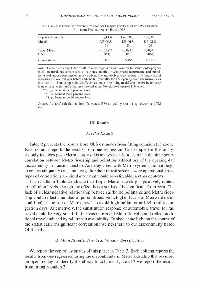
Table 3—The Effect of Metro Opening on Transportation Source Pollutants: Ridership Discontinuity Based OLS
Dependent variable: Log(CO) Log(NOx) Log(O3)Model: DB-OLS DB-OLS DB-OLS
(1) 2) (3)Taipei Metro Open
−0.156**(0.059)
−0.083(0.052)
−0.037(0.063)
Observations 17,076 16,466 17,070
Notes: Each column reports the result from one regression with controls for a third-order polyno-mial time trend, gas content regulation events, quartics in wind speed, temperature, and humid-ity, as well as, one hour lags of these variables. The unit of observation is hour. The sample for all regressions is one full year before and one full year after the TM opening date. The main entries in columns 1, 2 and 3 report the coefficient estimate from fitting model 2 in the text by ordinary least squares, with standard errors clustered at the 5-week level reported in brackets.
*** Significant at the 1 percent level. ** Significant at the 5 percent level. * Significant at the 10 percent level.
source: Authors’ calculations from Taiwanese EPA air quality monitoring network and TM data.
VoL. 4 No. 1 75CHEN ANd WHALLEy: GrEEN INfrAsTruCTurE
Table 3 contains two central findings. First, the point estimates indicate that the opening of the Metro substantially reduced emissions from one automobile source, CO. The results in column 1 indicate that the opening of the Taipei Metro reduced CO pollution by more than 15 percent and this result is statistically significant at the 5 percent level. The point estimate in column 2 indicates that the opening of the Taipei Metro reduced N O x pollution by 8 percent, but this point estimate is not sta-tistically significant at the 5 percent level. Thus, the opening of the Taipei Metro has a statistically significant effect of reducing pollution from key transportation based pollutant, carbon monoxide.
Second, Taipei Metro’s opening had little effect on air pollution from O 3 . The point estimate in column 3 does indicate that the opening of the Taipei Metro reduced O 3 , but the results are not statistically significant at any conventional level of statis-tical significance. As the health consequences of ground level ozone exposure are quite significant, this lack of effect on ozone pollution is notable.
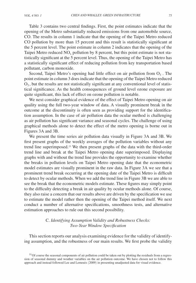
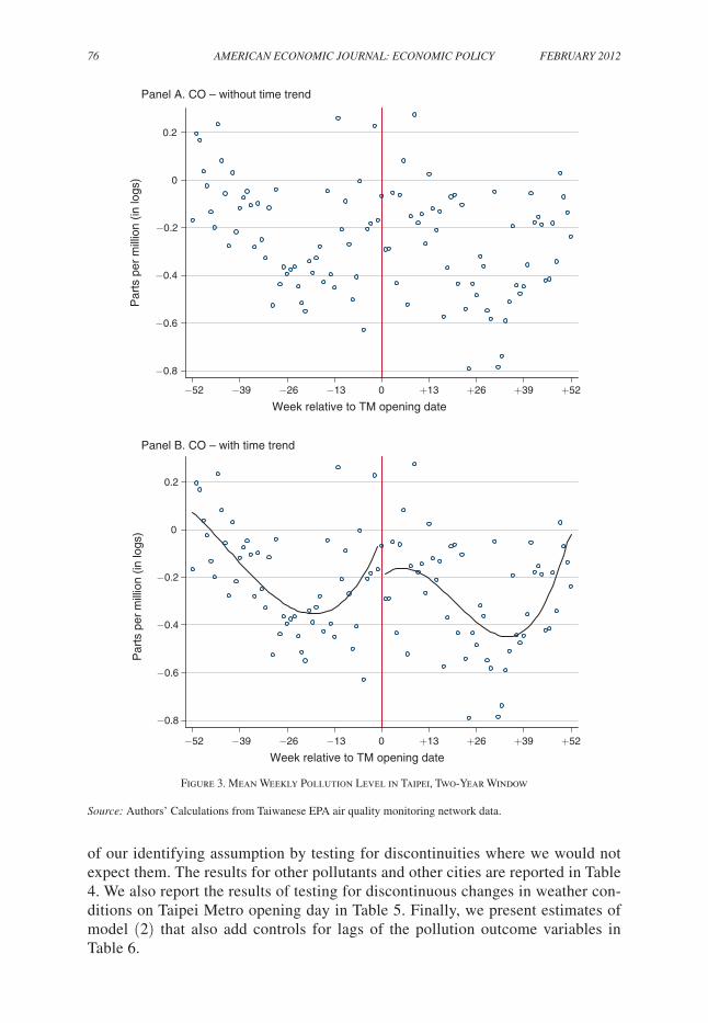
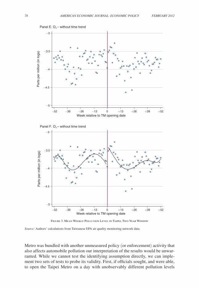
We next consider graphical evidence of the effect of Taipei Metro opening on air quality using the full two-year window of data. A visually prominent break in the outcome at the discontinuity is often seen as providing support for the identifica-tion assumption. In the case of air pollution data the ocular method is challenging as air pollution has significant variance and seasonal cycles. The challenge of using graphical methods alone to detect the effect of the metro opening is borne out in Figures 3A and 3B.
We present the time series air pollution data visually in Figure 3A and 3B. We first present graphs of the weekly averages of the pollution variables without any trend line superimposed.25 We then present graphs of the data with the third-order trend line and break at the Taipei Metro opening date superimposed. Displaying graphs with and without the trend line provides the opportunity to examine whether the breaks in pollution levels on Taipei Metro opening date that the econometric model estimates are visually prominent in the raw data. In Figure 3A we see that a prominent trend break occurring at the opening date of the Taipei Metro is difficult to detect by ocular methods. When we add the trend line in Figure 3B we are able to see the break that the econometric models estimate. These figures may simply point to the difficulty detecting a break in air quality by ocular methods alone. Of course, they also raise a concern that our results above are driven by the specification we use to estimate the model rather then the opening of the Taipei method itself. We next conduct a number of alternative specifications, smoothness tests, and alternative estimation approaches to rule out this second possibility.
C. Identifying Assumption Validity and robustness Checks: Two-year Window specification
This section reports our analysis examining evidence for the validity of identify-ing assumption, and the robustness of our main results. We first probe the validity
25 Of course the seasonal components of air pollution could be taken out by plotting the residuals from a regres-sion of seasonal dummy and weather variables on the air pollution outcome. We have chosen not to follow this approach and instead followed Lee and Lemeuix (2009) in presenting unadjusted data for visual evidence.
76 AMErICAN ECoNoMIC JourNAL: ECoNoMIC PoLICy fEBruAry 2012
of our identifying assumption by testing for discontinuities where we would not expect them. The results for other pollutants and other cities are reported in Table 4. We also report the results of testing for discontinuous changes in weather con-ditions on Taipei Metro opening day in Table 5. Finally, we present estimates of model (2) that also add controls for lags of the pollution outcome variables in Table 6.
Figure 3. Mean Weekly Pollution Level in Taipei, Two-Year Window
source: Authors’ Calculations from Taiwanese EPA air quality monitoring network data.
Panel A. CO – without time trend
−0.8
−0.6
−0.4
−0.2
0
0.2P
arts
per
mill
ion
(in lo
gs)
−52 −39 −26 −13 0 +13 +26 +39 +52
Week relative to TM opening date
Panel B. CO – with time trend
−0.8
−0.6
−0.4
−0.2
0
0.2
Par
ts p
er m
illio
n (in
logs
)
−52 −39 −26 −13 0 +13 +26 +39 +52
Week relative to TM opening date

VoL. 4 No. 1 77CHEN ANd WHALLEy: GrEEN INfrAsTruCTurE
A central potential concern for our identifying assumption is that the opening date of the Taipei Metro was not chosen randomly. As noted above, if officials wished to open the Taipei Metro on either a high or low travel day, were able to do so, and were able to accurately predict the level of travel on a given day, our iden-tifying assumption may be threatened. Alternatively, if the opening of the Taipei
Figure 3. Mean Weekly Pollution Level in Taipei, Two Year Window
source: Authors’ calculations from Taiwanese EPA air quality monitoring network data.
Panel C. NOx – without time trend
−4.5
−4
−3.5
−3
−2.5P
arts
per
mill
ion
(in lo
gs)
−52 −39 −26 −13 0 +13 +26 +39 +52
Week relative to TM opening date
Panel D. NOx – with time trend
−4.5
−4
−3.5
−3
−2.5
Par
ts p
er m
illio
n (in
logs
)
−52 −39 −26 −13 0 +13 +26 +39 +52
Week relative to TM opening date
78 AMErICAN ECoNoMIC JourNAL: ECoNoMIC PoLICy fEBruAry 2012
Metro was bundled with another unmeasured policy (or enforcement) activity that also affects automobile pollution our interpretation of the results would be unwar-ranted. While we cannot test the identifying assumption directly, we can imple-ment two sets of tests to probe its validity. First, if officials sought, and were able, to open the Taipei Metro on a day with unobservably different pollution levels
Figure 3. Mean Weekly Pollution Level in Taipei, Two-Year Window
source: Authors’ calculations from Taiwanese EPA air quality monitoring network data.
Panel E. O3 – without time trend
−5
−4.5
−4
−3.5
−3
Par
ts p
er m
illio
n (in
logs
)
−52 −39 −26 −13 0 +13 +26 +39 +52
Week relative to TM opening date
−5
−4.5
−4
−3.5
−3
Par
ts p
er m
illio
n (in
logs
)
−52 −39 −26 −13 0 +13 +26 +39 +52Week relative to TM opening date
Panel F. O3 – without time trend
VoL. 4 No. 1 79CHEN ANd WHALLEy: GrEEN INfrAsTruCTurE
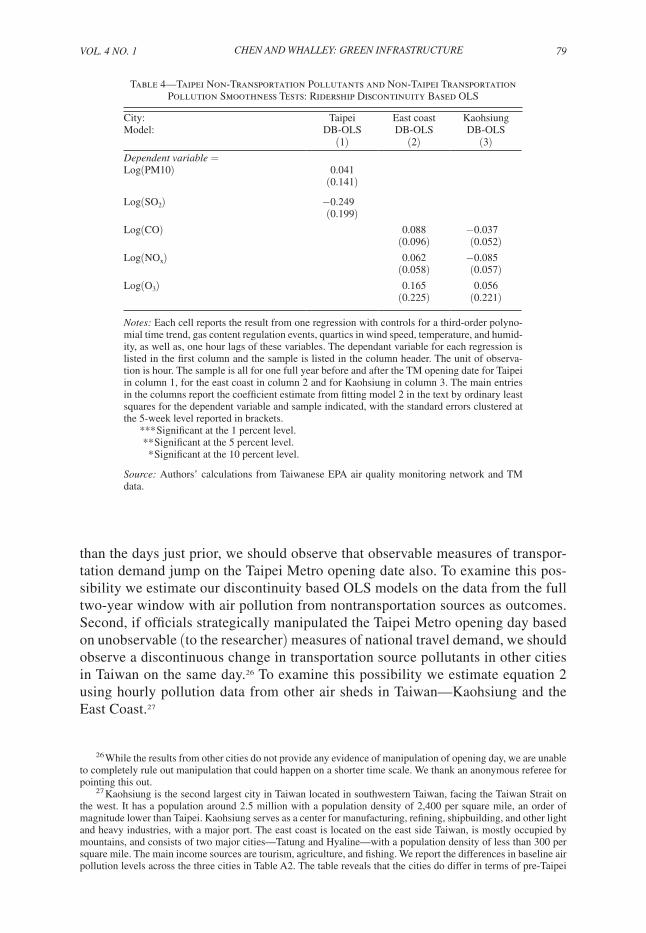
than the days just prior, we should observe that observable measures of transpor-tation demand jump on the Taipei Metro opening date also. To examine this pos-sibility we estimate our discontinuity based OLS models on the data from the full two-year window with air pollution from nontransportation sources as outcomes. Second, if officials strategically manipulated the Taipei Metro opening day based on unobservable (to the researcher) measures of national travel demand, we should observe a discontinuous change in transportation source pollutants in other cities in Taiwan on the same day.26 To examine this possibility we estimate equation 2 using hourly pollution data from other air sheds in Taiwan—Kaohsiung and the East Coast.27
26 While the results from other cities do not provide any evidence of manipulation of opening day, we are unable to completely rule out manipulation that could happen on a shorter time scale. We thank an anonymous referee for pointing this out.
27 Kaohsiung is the second largest city in Taiwan located in southwestern Taiwan, facing the Taiwan Strait on the west. It has a population around 2.5 million with a population density of 2,400 per square mile, an order of magnitude lower than Taipei. Kaohsiung serves as a center for manufacturing, refining, shipbuilding, and other light and heavy industries, with a major port. The east coast is located on the east side Taiwan, is mostly occupied by mountains, and consists of two major cities—Tatung and Hyaline—with a population density of less than 300 per square mile. The main income sources are tourism, agriculture, and fishing. We report the differences in baseline air pollution levels across the three cities in Table A2. The table reveals that the cities do differ in terms of pre-Taipei
Table 4—Taipei Non-Transportation Pollutants and Non-Taipei Transportation Pollution Smoothness Tests: Ridership Discontinuity Based OLS
City: Taipei East coast KaohsiungModel: DB-OLS DB-OLS DB-OLS
(1) (2) (3)dependent variable =Log(PM10) 0.041
(0.141)
Log(SO2) −0.249(0.199)
Log(CO) 0.088(0.096)
−0.037(0.052)
Log(NOx) 0.062(0.058)
−0.085(0.057)
Log(O3) 0.165(0.225)
0.056(0.221)
Notes: Each cell reports the result from one regression with controls for a third-order polyno-mial time trend, gas content regulation events, quartics in wind speed, temperature, and humid-ity, as well as, one hour lags of these variables. The dependant variable for each regression is listed in the first column and the sample is listed in the column header. The unit of observa-tion is hour. The sample is all for one full year before and after the TM opening date for Taipei in column 1, for the east coast in column 2 and for Kaohsiung in column 3. The main entries in the columns report the coefficient estimate from fitting model 2 in the text by ordinary least squares for the dependent variable and sample indicated, with the standard errors clustered at the 5-week level reported in brackets.
*** Significant at the 1 percent level. ** Significant at the 5 percent level. * Significant at the 10 percent level.
source: Authors’ calculations from Taiwanese EPA air quality monitoring network and TM data.
80 AMErICAN ECoNoMIC JourNAL: ECoNoMIC PoLICy fEBruAry 2012
Table 4 reports the results of our tests for discontinuities in observable measures of travel demand in Taipei on Taipei Metro opening day in column 1. Comfortingly, we find little evidence of discontinuities on Taipei Metro opening day in Taipei for either primarily industry source pollutants. Columns 2 and 3 of Table 4 report the results from the tests of fitting equation 2 to data on air pollution on the East Coast and in Kaohsiung (Taiwan’s second largest city). East Coast cities and Kaohsiung are located far from the Metro Taipei area, and so air quality is not expected to be affected by the Taipei Metro opening directly, but will be affected by any national changes in unobserved determinants of pollution due to changes in regulatory enforcement or economic activity, for example. Overall, we find little evidence for a large disconti-nuity in pollution on Taipei Metro opening date in other cities. These findings lend further credence to the validity of our identifying assumption, however concerns about whether our results are driven by unusual weather conditions remain.
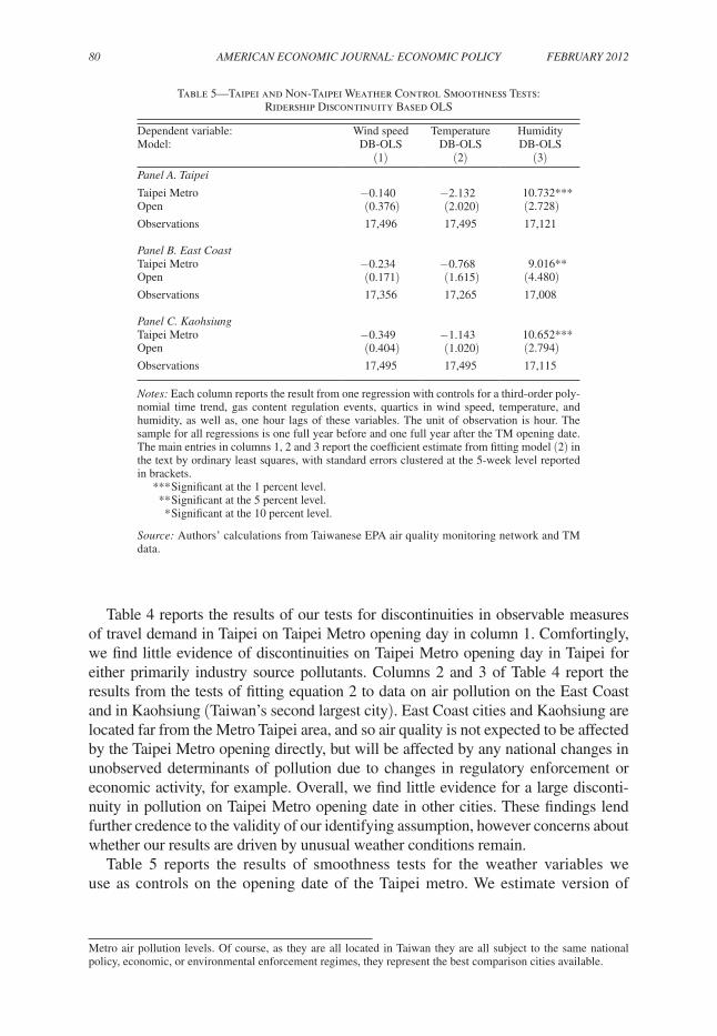
Table 5 reports the results of smoothness tests for the weather variables we use as controls on the opening date of the Taipei metro. We estimate version of
Metro air pollution levels. Of course, as they are all located in Taiwan they are all subject to the same national policy, economic, or environmental enforcement regimes, they represent the best comparison cities available.
Table 5—Taipei and Non-Taipei Weather Control Smoothness Tests: Ridership Discontinuity Based OLS
Dependent variable: Wind speed Temperature HumidityModel: DB-OLS DB-OLS DB-OLS
(1) (2) (3)Panel A. Taipei
Taipei MetroOpen
−0.140(0.376)
−2.132(2.020)
10.732***(2.728)
Observations 17,496 17,495 17,121
Panel B. East CoastTaipei MetroOpen
−0.234(0.171)
−0.768 (1.615)
9.016**(4.480)
Observations 17,356 17,265 17,008
Panel C. KaohsiungTaipei MetroOpen
−0.349(0.404)
−1.143(1.020)
10.652***(2.794)
Observations 17,495 17,495 17,115
Notes: Each column reports the result from one regression with controls for a third-order poly-nomial time trend, gas content regulation events, quartics in wind speed, temperature, and humidity, as well as, one hour lags of these variables. The unit of observation is hour. The sample for all regressions is one full year before and one full year after the TM opening date. The main entries in columns 1, 2 and 3 report the coefficient estimate from fitting model (2) in the text by ordinary least squares, with standard errors clustered at the 5-week level reported in brackets.
*** Significant at the 1 percent level. ** Significant at the 5 percent level. * Significant at the 10 percent level.
source: Authors’ calculations from Taiwanese EPA air quality monitoring network and TM data.

VoL. 4 No. 1 81CHEN ANd WHALLEy: GrEEN INfrAsTruCTurE
equation (2) with the indicated weather variable as the outcome and all weather controls dropped from the specification. We report estimates of the models for Taipei, Kaohsiung, and the East Coast. The results in Table 5 show that wind speed and temperature change smoothly on the Taipei Metro opening date in all three cities. Humidity however does not change smoothly on Taipei Metro opening day in any of the cities. Ideally all the weather controls would change smoothly at the discontinuity, however we feel the discontinuous change in humidity is not a major problem in this context for two reasons. First, wind speed and temperature have more explanatory power for air pollution than humidity. Second, the CO results in the last row of online Appendix Table A1 of model (2) without humidity covari-ates are very similar with a slightly smaller to those above in magnitude, but at 10 percent comfortably within the range we note above, and remain statistically significant at the 10 percent level. However, as Table 5 reveals that not all of the control variables are smooth on opening day we present further estimates that use only the 30-day window around opening day without any weather control variables to further address this potential concern in the subsection D.
One additional issue to examine in a time-series discontinuity based approach is how persistence in air pollution affects the magnitude of the metro opening
Table 6—The Effect of Metro Opening on Transportation Source Pollutants: Ridership Discontinuity Based OLS, Lagged Outcome Controls
Dependent variable: Log(CO) Log(NOx) Log(O3)Model: DB-OLS DB-OLS DB-OLS
(1) (2) (3)Taipei MetroOpen
−0.035**(0.015)
−0.028*(0.014)
−0.001(0.016)
First lag 1.092***(0.020)
0.922***(0.031)
0.686***(0.039)
Second lag −0.332***(0.026)
−0.092*(0.032)
0.220***(0.021)
Third lag 0.052**(0.015)
−0.007(0.013)
−0.027*(0.016)
Fourth lag −0.005(0.006)
−0.020**(0.007)
−0.096***(0.007)
Observations 17,072 14,027 17,042Cumulative effect of Taipei Metro open −0.141 −0.105 −0.003
Notes: Each column reports the result from one regression with controls for a third-order poly-nomial time trend, gas content regulation events, quartics in wind speed, temperature, and humidity, as well as, one hour lags of these variables. The unit of observation is hour. The sample for all regressions is one full year before and one full year after the TM opening date. The main entries in columns 1, 2 and 3 report the coefficient estimate from fitting model (2) in the text by ordinary least squares, with standard errors clustered at the 5-week level reported in brackets.
*** Significant at the 1 percent level. ** Significant at the 5 percent level. * Significant at the 10 percent level.
source: Authors’ calculations from Taiwanese EPA air quality monitoring network and TM data.
82 AMErICAN ECoNoMIC JourNAL: ECoNoMIC PoLICy fEBruAry 2012
effect.28 While clustering the standard errors at the 5 week level addresses for the effects of persistence on inference, it is well worth examining whether con-trolling for shorter-term lags substantially affects the point estimate results. As Henderson (1996) notes, ozone concentrations in the United States persist for 4 hours. Thus, we estimate (2) with controls for 1, 2, 3, and 4 hour lags of the pollu-tion outcome added. The results of these estimates are presented in Table 6. Table 6 demonstrates that adding lagged pollution measures has little effect on the sign or statistical significance of the metro opening effect, as both the CO and N O x results demonstrate. The magnitude of the point estimates are indeed smaller than in Table 3, as would be expected. The models in Table 3 reflect the total effect of the metro opening between the pre-TM pollution and post-TM pollution levels, whereas the point estimate in the Table 6 reflect only the very short-term effect. To make the estimates comparable we solve for the total effect of the metro open-ing by iteratively substituting into the lagged version of equation (2) and present the results in the last column of Table 6.29 The total Taipei Metro opening effect estimates in the last row of Table 6 are very close to those reported above indi-cating that persistence in air pollution does little to alter the magnitude of the air effects in this context.
We also examine in the supplementary Appendix the robustness of our results along three dimensions: reporting, polynomial order specification, and covariate choice. These results reported in Table A1 show that our CO results from the two-year window discontinuity based OLS specification are highly robust in general, while the estimates for O3 and N O x pollution outcome are more sensitive to speci-fication choices.30
D. Main results: 30-day Window specification
In this subsection we consider two further specifications that use only the obser-vations within 30 days of the Taipei Metro opening date.31 First, in Table 7 we report the results of estimating equation (2) without any weather, regulation, or time trend controls. Second, we report estimates from a simple difference-in-differences model that compares the change in air pollution before and after the Taipei metro opening in Taipei where the metro opens to Kaohsiung where there is no change in transpor-tation infrastructure in Table 8.
28 We thank an anonymous referee for this suggestion.29 We express the lagged version of equation (2) as:
y t = δ 0 + δ 1 Metroope n t + δ 2 x t + δ 3 P(t) + δ 4 P(t) × Metroope n t + β 1 y t−1 + β 2 y t−2 + β 3 y t−3 + β 4 y t−4 + e t .
Following Henderson (1996), we stack the equations for y t to y t−4 and recursively substitute for the lagged outcomes to obtain the total effect of the metro opening, δ 1
TE . We obtain the expression δ 1 TE = [1 + β 1 + β 1
2 + β 1
3 + β 1 4 + 3( β 1
2 β 2 ) + 2( β 1 β 2 ) + 2( β 1 β 3 ) + β 2 + β 2 2 + β 3 + β 4 ]x δ 1 = γ × δ 1 . We refer to γ as the multiplier for
the total effect. Based on the estimates of β 1 , β 2 , β 3 , and β 4 for each pollutant in Table 6 we obtain γ Co = 4.03, γ N o x = 3.75, and γ o 3 = 3.42. With these multipliers in hand the total effect of the metro opening (reported in the last row of Table 6) are obtained by multiplying the relevant γ multiplier times the relevant δ 1 estimate.
30 The supplementary Appendix is available at: faculty.ucmerced.edu/awhalley/.31 We thank an anonymous referee for suggesting this alternative narrow window specification.
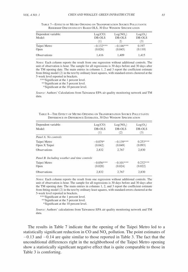
VoL. 4 No. 1 83CHEN ANd WHALLEy: GrEEN INfrAsTruCTurE
The results in Table 7 indicate that the opening of the Taipei Metro led to a statistically significant reduction in CO and N O x pollution. The point estimates of −0.13 and −0.14 are quite similar to those reported in Table 3. The fact that the unconditional differences right in the neighborhood of the Taipei Metro opening show a statistically significant negative effect that is quite comparable to those in Table 3 is comforting.
Table 8—The Effect of Metro Opening on Transportation Source Pollutants: Difference-in-Difference Estimates, 30 Day Window Specification
Dependent variable: Log(CO) Log(NOx) Log(O3)Model: DB-OLS DB-OLS DB-OLS
(1) (2) (3)Panel A. No controls
Taipei MetroOpen X Taipei
−0.079*(0.042)
−0.139***(0.049)
0.253***(0.093)
Observations 2,832 2,767 2,830
Panel B. Including weather and time controls
Taipei Metro Open
−0.056***(0.020)
−0.101***(0.024)
0.232***(0.022)
Observations 2,832 2,767 2,830
Notes: Each column reports the result from one regression without additional controls. The unit of observation is hour. The sample for all regressions is 30 days before and 30 days after the TM opening date. The main entries in columns 1, 2, and 3 report the coefficient estimate from fitting model (2) in the text by ordinary least squares, with standard errors clustered at the 5-week level reported in brackets.
*** Significant at the 1 percent level. ** Significant at the 5 percent level. * Significant at the 10 percent level.
source: Authors’ calculations from Taiwanese EPA air quality monitoring network and TM data.
Table 7—Effects of Metro Opening on Transportation Source Pollutants: Ridership Discontinuity Based OLS, 30 Day Window Specification
Dependent variable: Log(CO) Log(NOx) Log(O3)Model: DB-OLS DB-OLS DB-OLS
(1) 2) (3)Taipei Metro Open
−0.132***(0.026)
−0.146***(0.045)
0.197(0.110)
Observations 1,416 1,409 1,415
Notes: Each column reports the result from one regression without additional controls. The unit of observation is hour. The sample for all regressions is 30 days before and 30 days after the TM opening date. The main entries in columns 1, 2 and 3 report the coefficient estimate from fitting model (2) in the text by ordinary least squares, with standard errors clustered at the 5-week level reported in brackets.
*** Significant at the 1 percent level. ** Significant at the 5 percent level. * Significant at the 10 percent level.
source: Authors’ Calculations from Taiwanese EPA air quality monitoring network and TM data.
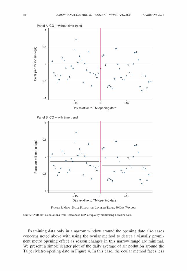
84 AMErICAN ECoNoMIC JourNAL: ECoNoMIC PoLICy fEBruAry 2012
Examining data only in a narrow window around the opening date also eases concerns noted above with using the ocular method to detect a visually promi-nent metro opening effect as season changes in this narrow range are minimal. We present a simple scatter plot of the daily average of air pollution around the Taipei Metro opening date in Figure 4. In this case, the ocular method faces less
Figure 4. Mean Daily Pollution Level in Taipei, 30 Day Window
source: Authors’ calculations from Taiwanese EPA air quality monitoring network data.
Panel A. CO – without time trend
Par
ts p
er m
illio
n (in
logs
)
−15 0 +15
Day relative to TM opening date
Panel B. CO – with time trend
Par
ts p
er m
illio
n (in
logs
)
−15 0 +15Day relative to TM opening date
1
0.5
0
−0.5
−1
1
0.5
0
−0.5
−1
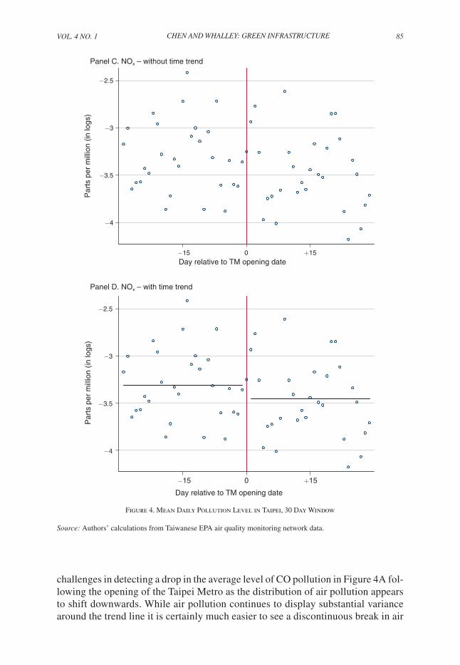
VoL. 4 No. 1 85CHEN ANd WHALLEy: GrEEN INfrAsTruCTurE
challenges in detecting a drop in the average level of CO pollution in Figure 4A fol-lowing the opening of the Taipei Metro as the distribution of air pollution appears to shift downwards. While air pollution continues to display substantial variance around the trend line it is certainly much easier to see a discontinuous break in air
Figure 4. Mean Daily Pollution Level in Taipei, 30 Day Window
source: Authors’ calculations from Taiwanese EPA air quality monitoring network data.
−2.5
−3
−3.5
−4
Panel C. NOx – without time trend
Par
ts p
er m
illio
n (in
logs
)
−15 0 +15Day relative to TM opening date
Panel D. NOx – with time trend
Par
ts p
er m
illio
n (in
logs
)
−15 0 +15
Day relative to TM opening date
−2.5
−3
−3.5
−4
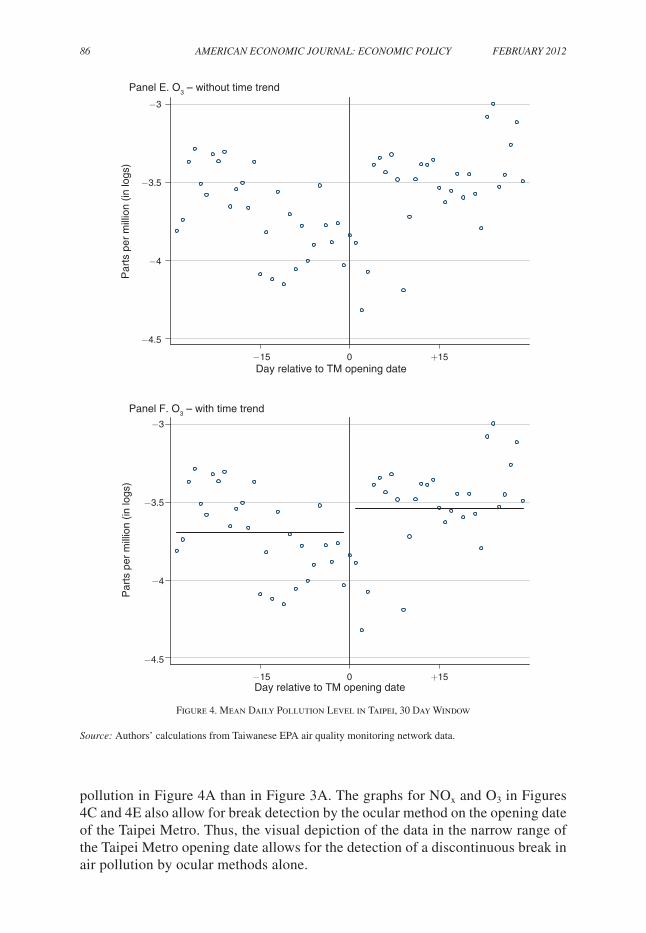
86 AMErICAN ECoNoMIC JourNAL: ECoNoMIC PoLICy fEBruAry 2012
pollution in Figure 4A than in Figure 3A. The graphs for N O x and O 3 in Figures 4C and 4E also allow for break detection by the ocular method on the opening date of the Taipei Metro. Thus, the visual depiction of the data in the narrow range of the Taipei Metro opening date allows for the detection of a discontinuous break in air pollution by ocular methods alone.
Figure 4. Mean Daily Pollution Level in Taipei, 30 Day Window
source: Authors’ calculations from Taiwanese EPA air quality monitoring network data.
−3
−3.5
−4
−4.5
Panel E. O3 – without time trend
Par
ts p
er m
illio
n (in
logs
)
−15 0 +15Day relative to TM opening date
Panel F. O3 – with time trend
Par
ts p
er m
illio
n (in
logs
)
−15 0 +15Day relative to TM opening date
−3
−3.5
−4
−4.5
VoL. 4 No. 1 87CHEN ANd WHALLEy: GrEEN INfrAsTruCTurE
In our last set of specifications we consider an alternative approach to forming the counterfactual of what would have happened to air pollution in Taipei if the metro had not opened. Here we use the trend in air pollution in Kaohsiung, the second largest city in Taiwan, to form the counterfactual in a simple difference in difference specification.32 The model RD-OLS model we estimate is given by,
(3) y t = δ 0 + δ 1 Metroope n t + δ 2 x t + δ 3 Taipei + δ 4 Taipei × Metroope n t + e t ,
where the coefficient of interest, δ 4 , is the effect of Taipei Metro’s opening on air pollution. Again, the variable Metroope n t is an indicator variable that takes a value of one for all hours after the Taipei Metro is operational and a value of zero before the Taipei Metro is operational. The vector of covariates, x t , includes indicator vari-ables for gas content regulations being in place and weather variables including current and 1-hour lags of quartics in temperature, wind speed, and humidity, in addition to, month, day of the week, hour fixed effects, a third order time trend, and the full set of interactions between hour and day of week fixed effects. The variable Taipei is a dummy variable that takes a value of one for air pollution monitoring sta-tion in Taipei and zero otherwise.33
The results for the difference-in-difference model are presented in Table 8. We first present results for specifications without any weather and time series controls in Panel A. We then present results of models that include controls for city weather conditions and time trends in Panel B to account for differences in weather condi-tions between the two cities. The broad pattern of results is very similar to those reported in Table 3 above. The point estimates indicate that the opening of the Taipei Metro reduced air pollution from CO and N O x , and increased air pollution from O 3 .
34 The magnitude of the point estimates do differ somewhat from those above. Compared to the results above the absolute value of the point estimates in Table 8 are smaller for CO, larger for N O x , and larger for O 3 . We take the results of differ-ence-in-difference specification to form the lower bound of the range of estimates noted in the introduction. The majority of estimates are statistically significant at the 5 percent level, with the exception of the CO estimate in Panel A that illustrates the precision gain from including the weather controls. Thus, the results in Table 8 indicate that the effect of Taipei Metro opening on CO pollution is robust alternative
32 We chose Kaohsiung as the control city for two reasons. First, it is a completely different airshed from Taipei and so air pollution there will not be directly affect by the opening of the Taipei Metro itself. Second, as the results in Table A2 demonstrate Kaohsiung is more comparable to Taipei in terms of baseline pollution levels than the East Coast (though many baseline levels are far from identical).
33 We continue to collapse the monitoring station data to one observation per city in an hour by taking the aver-age level of pollution across all monitoring stations in that city. We thus have two observations per hour, one for Taipei and one for Kaohsiung.
34 A positive estimate for Ozone is expected because Taipei has a VOC-limited climate leading to a negative relationship between N O x emissions and O 3 concentrations. Ozone is produced by a series of chemical reactions that involve nitrogen oxides (N O x ) and volatile organic compounds (VOCs) in the presence of sunlight and heat. The formation involves highly nonlinear and complicated processes, depending on the relative forcing of various chemical species and local meteorological conditions that could vary over space and time (Seinfeld and Pandis 1998). Overall in urban areas, such as Taipei, which O 3 formation is VOC-limited, implying that a reduction in N O x emissions would increase O 3 concentrations. On the other hand in the VOC-limited climate, O 3 concentrations will decrease if N O x emissions increase.
88 AMErICAN ECoNoMIC JourNAL: ECoNoMIC PoLICy fEBruAry 2012
formulations of the counterfactual, even though they indicate the effect is smaller then those reported above.
E. Estimate Magnitudes
Implied Behavioral responses.—Are CO effects of the magnitudes we find plau-sible? One way to think about the answer is to compute the implied traffic diversion ratio away from automobile travel towards rail transit. As the emissions inventory indicates that virtually all CO emissions are transportation based, our estimates can be interpreted as an approximation of the percentage change in automobile vehicle miles travelled from the opening of the Taipei Metro. To compute the traffic diver-sion ratio, we then need to compute the ratio of the daily number of Taipei Metro trips in Table 1 of 40,000 to the number of total automobile commuting trips in Taipei before the Taipei Metro. Unfortunately, this simple calculation proves diffi-cult as detailed transportation mode utilization data are unavailable for Taipei before the Taipei Metro opened. However, we can infer the number of automobile trips before the Taipei Metro by using 2001 mode share data in concert with an estimate of the total number of commuters before the Taipei Metro opened. Doing so we obtain an estimate of 375,000 automobile trips per day in Taipei before the Taipei Metro opened.35 The daily Taipei Metro ridership is just over 10 percent of the auto-mobile trips. Our estimated effect strikes us as quite plausible as our estimated CO effects ranging from a 5 percent to 15 percent reduction in CO pollution contains this back of the envelope calculation of the percentage change of total automobile commute trips Taipei Metro ridership represents.
A second exercise is to calculate what the expected magnitude of a CO pollution response would be if Taipei had the same traffic diversion ratio as used in Parry and Small (2009) for Washington, DC. Conducting this calculation allows us to see whether our estimates are plausible based on the available estimates of the behav-ioral responses of automobile travelers to mass urban transit. Parry and Small (2009) use a traffic diversion ratios of 0.70 (peak) and 0.60 (off-peak) for Washington, DC. Multiplying these estimates by the observed number of daily trips on the Taipei Metro from Table 1 (40,000) we obtain estimates of the number of automobile trips diverted to the metro of 28,000 (peak) and 24,000 (off-peak). As virtually all of CO emissions are due to automobile trips we can estimate the expected CO effect by simply dividing the number of diverted trips by the total number of trips. Based on these calculations we would expect the Taipei Metro opening to reduce CO pol-lution by 7 percent (peak) to 6 percent (off-peak). Thus, these calculations lead to estimates that are smaller but close to our DB-OLS estimates and larger than our dif-ference-in-difference estimates. Again, as the range of our CO estimates contain an estimate derived from existing estimates of the behavioral response of automobile
35 According to a large sample survey of Taipei commuters in 1988, there were 250,000 people commuting daily in and out of Taipei city for a total of 500,000 trips per day (Chen 1992). We do not have access to mode-share data before the Taipei Metro, however, Jou et al. (2010) report that in 2001 in Taipei 75 percent of commuters used a car or motorbike as the primary travel modes. Together these estimates suggest that a rough estimate of the daily number of automobile trips, before the Taipei Metro opened, was approximately 375,000.
VoL. 4 No. 1 89CHEN ANd WHALLEy: GrEEN INfrAsTruCTurE
travel this calculation provides further reassurance that the magnitudes of estimated pollution effects are plausible.
Economic significance.—It is also interesting to ask, how large are air quality benefits we estimate in economic terms? One way to assess the size of the benefit of our estimates is to first calculate the effects of the reduction in CO pollution due to Taipei Metro ridership focusing on the well documented health effects.36 To make this comparison we proceed in two steps. We first calculate the magnitude of the health effects that our CO estimates imply. We then scale the health effect benefits by the Metro ridership per mile so that a comparison to the estimates in Small and Parry (2009) is possible.37
We first use the recent estimates of the health effects of air pollution to calculate the implied health benefits of the Taipei Metro opening. Recent work by Currie, Neidell, and Schmieder (2009) finds that a one ppm reduction in CO reduced infant mortality by 2.5 percent in proportion to the baseline risk, accounting for avoid-ance behavior.38 Focusing very narrowly on infant mortality health effects only we obtain estimates of 1.7 lives saved valued at $8.7 Million USD in the first year of Taipei Metro operation using our baseline estimates.39 More broadly, and perhaps speculatively, if we apply the infant mortality estimate to the elderly population who are also at risk of mortality from air pollution exposure we obtain an estimate of 58 elderly lives saved, leading to a total value of all lives saved of around $85.2 Million USD in the first year of Taipei Metro operation.40
36 While the epidemiological literature has carefully estimated relationships between air pollution and a range of health outcomes, the avoidance behavior of optimizing individuals is typically not accounted for (Dockery et al. 1993; Samet et al. 2000; Bell et al. 2004). As the economics literature has demonstrated that accounting for avoid-ance behavior is important, estimates that account for avoidance are preferred to understand the magnitude of the health effects of air pollution (Neidell 2004, 2009, and Moretti and Neidell 2008). We thus focus on using estimates that account for avoidance behavior in estimating the welfare consequences of Taipei Metro ridership.
37 An implicit assumption with our calculation of the health effects implied by the air quality benefits is that the majority of the pollution in Taipei is from sources in Taipei itself. Certainly, the air pollution from the neigh-boring areas is likely to affect the air quality in Taipei. However, as Taipei has a basin-type topology (similar to Los Angeles) it is an independent airshed, so that the effect of nonlocal activity on air pollution is relatively minor compared to the local source activity (Chang and Lee 2006). We thank an anonymous referee for pointing out this implicit assumption in our calculation.
38 We are unaware of studies of other health effects of CO exposure that account for avoidance behavior. However, one recent study of the effects of CO exposure of asthma incidence suggests that nonmortality effects are likely to be small. For example, the estimates in Clark et al. (2010) allow us to get a sense of how large the reduc-tions in asthma would be. To calculate incremental risk associated with 1ppm of CO, we assume that asthma is rare so that the odds ratio is a good approximation of the relative risk. Given that we do not have access to data on the baseline incidence of asthma, we used prevalence of (4.5 percent) as a surrogate (Lee et al. 2007). Under these assumptions, our calculation shows that the Taipei Metro reduced lifetime asthma by 234 cases per year (=(1 − 1/ e 0.834ppm×0.7745×0.157 ) × 0.045 × 77,209). As the annual health cost of a patient with asthma in Taiwan is estimated to be $260 (Sun et al. 2007) higher than that of a patient without asthma, the economic benefit of these avoided asthma related health care costs is estimated to be roughly $57,000 per year.
39 In 1996 there were 77,029 infants (children less than one year) with a mortality rate of 6.66 per 1000 infants in the Taipei Metro area according to census data. Thus, our baseline estimates of the reduction in CO caused by Taipei Metro ridership of 15.6 percent, yields an estimated reduction in infant deaths in Taipei of about 1.7 (=0.834ppm × 0.156 × 0.025 × 0.00666 × 77,029) in the first year of operation. We apply the value of $4.87 million per life used in Small and Kazimi (1995) for comparison purposes as this estimate is utilized in total benefit of mass transit calculations in Small and Perry (2009) enabling comparisons to be made on an equal footing. It is important to note however that this value of a statistical life is significantly larger than that estimated for Taiwan. Liu and Hammitt (1999) estimate the statistical value life for Taiwan as being $1.2 million.
40 To calculate the number of elderly lives saved we use the mortality rate, excluding accidents, for elder popula-tion of roughly 4,275 per 100,000, and the number of elders is 422,995 in the Metropolitan Taipei area according to
90 AMErICAN ECoNoMIC JourNAL: ECoNoMIC PoLICy fEBruAry 2012
To complete the comparison, we next express the air pollution benefit of rail tran-sit infrastructure in terms of cents per passenger mile. Doing so yields an implied local air pollution benefit of between 6.4 and 62.7 cents per passenger mile.41 This is significantly larger than what prior work would imply. The calculations in Parry and Small (2009) are based on an external costs of automobile travel from local pol-lution of 2.0 cents per mile (Parry and Small 2009, App-13, and Small and Kazimi 1995). Dividing the per mile vehicle local air pollution cost by the average modal diversion rate for Washington, DC (Parry and Small 2009, Table 2) of 0.65 leads to an implied air pollution benefit of 3 cents per passenger mile of rail transit, less than half of what we find for our infant only calculation.
In addition, the air quality effects we measure here represent a sizable compo-nent of the total benefits of rail transit infrastructure calculated by Parry and Small (2009). Again for the Washington DC Metro, Parry and Small (2009) report overall social values of 19.8 (peak) and 13.9 (off-peak) cents per passenger mile. Our esti-mates of 5.4 cents per passenger mile imply that the air quality effects account for between 32 and over 450 percent of the social value of rail transit they compute. Indeed, our (more speculative) upper bound calculations suggest that the air quality effects of rail transit may be an order of magnitude larger than the total social value of rail transit computed in prior work. Regardless of the precise method used to interpret the magnitude of the air quality benefits, our estimated effects are signifi-cantly larger than those in prior work, and indicate that the air quality effects of rail transit infrastructure are economically substantial.
Of course our calculation is subject to many limitations. In one sense, our calcu-lation is likely to represent a lower bound estimate of the full benefit of enhanced air quality as it does not include the full range of potential health effects or include the social costs of avoidance behavior. It is also possible that the effects of CO on health in Taipei could differ from those in the United States, where the data underlying the health effect estimates we employ are based. Furthermore, the long-run substitution response towards the metro could well be larger than the short run response underly-ing the estimates here.
However, our calculation may represent an upper bound to the long-term health effects of a metro system. This would be the case if the substitution away from non-travel activities toward travel caused by the metro opening took substantial time. For example, as the metro system leads to substitution away from automobile travel con-gestion on the roads is reduced. If potential travelers learn of the congestion reduction over time and respond by driving more total traffic levels may fall less in the long term than the short term. To the extent that the effects of rail transit on travel time are
census data. With these numbers in hand our estimate of the reduction in CO caused by the Taipei Metro ridership yields an estimated reduction in elder deaths of 58.8 cases (= 0.834ppm × 0.156 × 0.025 × 0.04275 × 422,995) As those older than 65 have a much shorter life remaining we apply the adjustment for life expectancy formula in Aldy and Viscusi (2007, p. 8) with their suggested value of a year of life of $300,000, a remaining life for the over 65 in Taiwan of 5 years, and a discount rate of 5 percent. Doing so yields a statistical value of remaining life for this population of $1.3 Million, and a total value of the reduction in mortality of $76.4 Million for the over-65 population.
41 The exact calculation of the air quality benefit in cents per passenger mile = totalbenefit
___ [trips/day] × [days/year] × [milesoftrack] .
The infant health effect = 8.6M __
40, 000 × 365 × 9.3 = 0.063. The infant and elderly effect is = 85.2M
__ 40, 000 × 365 × 9.3
= 0.627.
VoL. 4 No. 1 91CHEN ANd WHALLEy: GrEEN INfrAsTruCTurE
expected, our estimates will incorporate the short run adjustment responses of workers and firms, such as changes in work schedules. However, as some of the adjustments to rail transit infrastructure may take time (such as changes in land use), longer term traffic creation responses may well be larger than the shorter term traffic creation responses in our estimates. As the best available estimates of traffic creation (i.e. that account for the endogenous location of highway capacity) indicate that the majority of traffic creation occurs in the short term our estimates likely capture much of the traffic creation effect. These estimates indicate that the short term traffic creation elasticity (0.54) is about two thirds of the longer term traffic creation elasticity (0.78–0.84), and that the long-run elasticity is less than one (Cervevo 2002).42
While we regard our results as being informative about the effects urban rail transit in air quality over more than the very short term, it is important to be clear about the limitations in applying our estimates over a much longer time period. One central limitation is that our estimates do not capture any sorting responses to local public good provision (i.e., Seig, Smith, Banzhaf, and Walsh 2004). These sorting responses have been shown to be important for large scale urban transit projects in particular. As Kahn (2007) and Glaeser, Kahn, and Rappaport (2008) demonstrate that urban transit infrastructure projects tend to tend to attract a lower income popu-lation who do not own vehicles. The effects of these types of sorting responses on air quality are not entirely clear. On one hand, a lower income population might travel more by public transit and less by private vehicles so that the sorting responses lead to further negative impacts on local air pollution. On the other hand, population density is likely to increase with the reduction in average income which could lead to additional private vehicle travel in the area. In any case, we are able to say little about population sorting responses in the analysis here and leave the question of whether sorting attenuates or amplifies the air quality effects of urban rail transit we document for future research.
F. Heterogeneous Effects
The results thus far have demonstrated an important effect of the Metro’s open-ing on average level of tailpipe air pollution in Taipei. In the next subsection we examine whether there is any evidence of heterogeneous effects of the Taipei Metro opening. We first examine whether there are any distributional effects of the metro opening by examining whether neighborhoods with a larger number of households in poverty experience especially large or small metro opening effects. To do so, we classify each pollution monitoring station as being above or below median pov-erty level and interact the high poverty indicator variable with the metro opening dummy.43 The results of this exercise are useful for understanding whether there are “environmental justice” implications of the results and are particularly worth
42 More recently, Duranton and Turner (2011) estimate a long run highway capacity traffic creation elasticity of one.
43 Unfortunately, after numerous attempts we were unable to obtain data on the characteristics of the population by neighborhood before the Taipei Metro opened. The reported results are based on the earliest year of neighbor-hood poverty data we were able to obtain, from 2006. Thus, the estimates may partially reflect sorting response to the metro opening in addition to the distributional effects of interest.
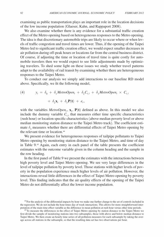
92 AMErICAN ECoNoMIC JourNAL: ECoNoMIC PoLICy fEBruAry 2012
examining as public transportation plays an important role in the location decisions of the low income population (Glaeser, Kahn, and Rappaport 2008).
We also examine whether there is any evidence for a substantial traffic creation effect of the Metro opening based on heterogeneous responses to the Metro opening. The idea is that discretionary automobile trips are likely to occur where or when lev-els of traffic congestion and travel times are lower. Thus, if the opening of the Taipei Metro led to significant traffic creation effect, we would expect smaller decreases in air pollution during off-peak hours or locations far from the central business district. Of course, if adjusting the time or location of travel time is quite costly for auto-mobile travelers then we would expect to see little adjustments made by optimiz-ing travelers. To shed some light on these issues we study whether travel patterns adapt to the availability of rail transit by examining whether there are heterogeneous responses to the Taipei Metro.
To conduct our analysis we simply add interactions to our baseline RD model above. Specifically, we fit the following model,
(4) y t = δ 0 + δ 1 Metroope n t + δ 2 C t, i + δ 3 Metroope n t × C t, i
+ δ 2 x t + δ 3 P(t) + e t ,
with the variables Metroope n t , x t , P(t) defined as above. In this model we also include the dummy variable C t, i that measures either time specific characteristics (rush hour) or location specific characteristics (above median poverty level or above median monitoring station distance to the Taipei Metro track). The coefficient esti-mate δ 3 measures whether there are differential effects of Taipei Metro opening by the relevant time or location.44
We present evidence for heterogeneous responses of tailpipe pollutants to Taipei Metro opening by monitoring station distance to the Taipei Metro, and time of day in Table 9.45 Again, each entry in each panel of the table presents the coefficient estimates with the outcome variable given in the column heading and the sample in the row heading.
In the first panel of Table 9 we present the estimates with the interactions between high poverty level and Taipei Metro opening. We see very large differences in the level of tailpipe pollution by poverty level. Those stations with higher levels of pov-erty in the population experience much higher levels of air pollution. However, the interactions reveal little differences in the effect of Taipei Metro opening by poverty level. This finding indicates that the air quality effects of the opening of the Taipei Metro do not differentially affect the lower income population.
44 For the analysis of the differential impacts by hour we make one further change to the set of controls included in the regression. We do not include the hour times day of week interactions. This allows for more straightforward inter-pretation of the main time effect variable as the difference in mean pollution at rush hour versus other time periods.
45 To measure the differences in the effect of Taipei Metro opening by station distance to the Taipei Metro we first divide the sample of monitoring stations into two subsamples, those with above and below median distance to Taipei Metro. We then create an hourly time series of all pollution measures for each subsample by taking the aver-age across all stations in the subsample, so that the resulting data set has two observations per hour.
VoL. 4 No. 1 93CHEN ANd WHALLEy: GrEEN INfrAsTruCTurE
In the second panel of Table 9 we present the estimates with the interactions between above median monitoring station distance from the Taipei Metro track and Taipei Metro opening. We see very large differences in the level of tailpipe pollution by distance to the Taipei Metro track. As expected, those stations located near the Taipei Metro track in the central business district experience much larger levels of air pollution. Most importantly, the interactions reveal little differences in the effect of Taipei Metro opening by distance to the Taipei Metro. This finding suggests that automobile travellers did not significantly alter their route of travel in response to the opening of the Taipei Metro.
In the third panel of Table 9 we examine whether the response of air quality to Taipei Metro opening differs during peak travel hours. Again, we see very large differ-ences in the level of tailpipe pollution between peak and nonpeak travel hours. Perhaps surprisingly, peak travel hours experience lower levels of tailpipe air pollution than other hours of the day, though this fact is likely due to the persistence in air pollution
Table 9—The Effect of Metro Opening on Primarily Transportation Source Pollutants, Heterogeneous Effects: Ridership Discontinuity Based OLS
Dependent variable: Log(CO) Log(NOx)Model: DB-OLS DB-OLS
(1) (2)Panel A. Poverty level
Metro open −0.086**(0.039)
0.034(0.100)
High poverty monitoring station −0.085***(0.016)
−0.471**(0.044)
Metro open × high poverty monitoring station 0.019(0.020)
0.004(0.073)
Panel B. station location
Metro open −0.129**(0.046)
−0.004(0.115)
Monitoring station close to metro 0.426***(0.013)
0.636***(0.043)
Metro open × monitoring station close to metro 0.040(0.035)
0.013(0.073)
Panel C. Time of dayMetro open −0.078**
(0.040)0.035
(0.119)Rush hour −0.144***
(0.049)−0.140*(0.073)
Metro open × rush hour 0.006(0.032)
0.034(0.049)
Notes: Each cell reports the result from one regression with controls for a third-order polyno-mial time trend, gas content regulation events, quartics in wind speed, temperature, and humid-ity, as well as, one hour lags of these variables. The unit of observation is hour. The sample is all observations for one full year before and after the TM opening date. The main entries in col-umns 1 and 2 report the coefficient estimate from fitting model (4) in the text by ordinary least squares, with the standard errors clustered at the 5-week level reported in brackets..
*** Significant at the 1 percent level. ** Significant at the 5 percent level. * Significant at the 10 percent level.
source: Authors’ calculations from Taiwanese EPA air quality monitoring network and TM data.
94 AMErICAN ECoNoMIC JourNAL: ECoNoMIC PoLICy fEBruAry 2012
noted above. We again see little evidence of a travel pattern response. The interac-tion effects are very small and statistically indistinguishable from zero at conventional statistical significance levels. Thus, it does not appear that automobile travelers sig-nificantly altered their time of travel in response to the opening of the Taipei Metro.
It is important to note an important limitation with using high frequency air pollu-tion data to measure high frequency travel behavior. As air pollution displays some persistence in the atmosphere, high frequency changes in air pollution may well understate high frequency changes in travel behavior. As such we regard the evi-dence reported in Table 9 on the heterogeneous effects as more suggestive than our main results above. Taking the results in Table 9 at face value the fact that we find little evidence of changes in automobile time or route of travel in response to the opening of the Metro could be due to two possibilities. First, it could be the case that because the opening and route of the Taipei Metro were known years in advance of opening day individuals already made adjustments to these travel pat-terns in advance of opening day. It could also be the case that adjustments in time or route of travel are costly. For example, if the costs of finding a new job with differ-ent work hours are meaningful, they may outweigh the benefits from adjustment in terms of reduced travel time. Of course, without additional evidence it is difficult to untangle the precise reason for the lack of adjustment in the time or route of travel.
IV. Conclusion
The transportation sector is a major source of air pollution worldwide. Recent evi-dence has indicated that automobile pollution poses significantly larger adverse health impacts than previously realized. Despite the importance of the transportation sector for air pollution, little work has examined the air pollution effects of transportation infrastructure directly. This paper seeks to fill the gap by examining the effects of one major type of transportation infrastructure—urban rail transit—on air quality.
Our analysis of the effects of the opening of a completely new Metro system in Taipei reveals three findings. First, we find that the opening of the Taipei Metro reduced air pollution from one tailpipe pollutant, carbon monoxide, by 5 to 15 percent. Our second set of findings shows little evidence that ground level ozone pollution is affected by the opening of the Taipei Metro however. Lastly, our results show little evi-dence of sizable travel pattern adjustments by automobile travelers in response to rail transit infrastructure. Importantly, the air quality effects we identify here for a large fraction of the total social value of rail transit infrastructure estimated in prior work. Thus, the air quality effects we measure here are important components of the benefits of rail transit infrastructure. Our results demonstrate that environmental effects can be important components of the social value of public infrastructure.
While this paper has reported new evidence on the environmental effects of rail transit infrastructure, it is natural to ask whether our results will carry over to other cities. Of course, the precise effects of rail transit infrastructure depend on many fac-tors, which may differ across areas. While it seems likely the differences in automo-bile technology can be accounted for relatively easily the portability of our estimates to other areas also depends on behavioral responses of travellers. A more definitive answer awaits compelling evidence for other areas.
VoL. 4 No. 1 95CHEN ANd WHALLEy: GrEEN INfrAsTruCTurE
There are several worthwhile directions for future research. First, applying a similar discontinuity approach to evaluate the air quality effects of other types of transport infrastructure would be fruitful. For example, the air quality effects of high speed rail or an airport infrastructure could be measured by using the opening of project that was subject to hard to predict construction delays. As a number of anecdotal accounts suggest that high-speed rail ridership has come in below expec-tations, the air quality effects of high speed rail might well be smaller than those documented here. Secondly, measuring the effects of transportation infrastructure on health outcomes directly would be very interesting, as the responsiveness of indi-vidual travel behavior to transportation infrastructure availability may depend partly on their underlying health conditions.
REFERENCES
Aldy, Joseph E., and W. Kip Viscusi. 2007. “Age Differences in the Value of Statistical Life: Revealed Preference Evidence.” review Environmental Economics and Policy, 1(2): 241–60.
Auffhammer, Maximilian, and Ryan Kellogg. Forthcoming. “Clearing the Air? The Effects of Gasoline Content Regulation on Air Quality.” American Economic review.
Baum-Snow, Nathaniel. 2007. “Did Highways Cause Suburbanization?” Quarterly Journal of Eco-nomics, 122(2): 775–805.
Baum-Snow, Nathaniel, and Matthew E. Kahn. 2005. “Effects of Urban Rail Transit Expansions: Evi-dence from Sixteen Cities, 1970–2000.” In Brookings-Wharton Papers on urban Affairs: 2005, ed. Gary T. Burtless and Janet Rothenberg Pack, 147–97. Washington, DC: Brookings Institution Press.
Bell, Michelle L., Aidan McDermott, Scott I. Zeger, Jonathan M. Samet, and Francesca Dominici. 2004. “Ozone and Short-term Mortality in 95 US Urban Communities, 1987–2000.” Journal of the American Medical Association, 292(19): 2372–78.
Borken, Jens, Heike Steller, Tamás Meretei, and Filip Vanhove. 2007. “Global and Country Inventory of Road Passenger and Freight Transportation, Fuel Consumption and Emissions of Air Pollutants in Year 2000.” Transportation research record: Journal of the Transportation research Board, 2011: 127–36.
Clark, Nina Annika, Paul A. Demers, Catherine J. Karr, Mieke Koehoorn, Cornel Lencar, Lillian Tam-buric, and Michael Brauer. 2010. “Effect of Early Life Exposure to Air Pollution on Development of Childhood Asthma.” Environmental Health Perspectives, 118(2): 284–90.
CCTV. 2009. “Beijing to Build ‘Public Transport City.’” June 10. http://www.cctv.com/english/special/excl/20090610/110347.shtml.
Cervero, Robert. 2002. “Induced Travel Demand: Research Design, Empirical Evidence, and Norma-tive Policies.” Journal of Planning Literature, 17(1): 3–20.
Chang, Shuenn-Chin, and Chung-Te Lee. 2006. “Ozone Variations through Vehicle Emissions Reduc-tions Based on Air Quality Monitoring Data in Taipei City, Taiwan, from 1994–2003.” Atmospheric Environment, 40(19): 3513–26.
Chay, Kenneth Y., and Michael Greenstone. 2003. “The Impact of Air Pollution on Infant Mortality: Evidence from Geographic Variation in Pollution Shocks Induced by a Recession.” Quarterly Jour-nal of Economics, 118(3): 1121–67.
Chen, Chao-Nan. 1992. “Extended Commuting and Migration in the Taipei Metropolitan Area.” Jour-nal of Population studies, (15): 161–83.
Chen, Yihsu, and Alexander Whalley. 2012. “Green Infrastructure: The Effects of Urban Rail Transit on Air Quality: Dataset.” American Economic Journal: Economic Policy. http://dx.doi.org/10.1257/pol.4.1.58.
Cohen, Aaron J., H. Ross Anderson, Bart Ostro, Kiran Dev Pandey, Michal Krzyzanowski, Nino Künzli, Kersten Gutschmidt, et al. 2004. “Urban Air Pollution.” In Comparative Quantification of Health risks: Global and regional Burden of disease Attributable to selected Major risk fac-tors, Vol. 1, ed. Majid Ezzati, Alan D. Lopez, Anthony Rodgers, and Christopher J. L., 1353–1434. Geneva: World Health Organization.
Cooper, Michael. 2010. “Administration Loosens Purse Strings for Transit Projects.” New york Times, January 13. http://www.nytimes.com/2010/01/14/us/14streetcar.html.
96 AMErICAN ECoNoMIC JourNAL: ECoNoMIC PoLICy fEBruAry 2012
Currie, Janet, and Matthew Neidell. 2005. “Air Pollution and Infant Health: What Can We Learn from California’s Recent Experience?” Quarterly Journal of Economics, 120(3): 1003–30.
Currie, Janet, Matthew Neidell, and Johannes F. Schmieder. 2009. “Air Pollution and Infant Health: Lessons from New Jersey.” Journal of Health Economics, 28(3): 688–703.
Currie, Janet, and Reed Walker. 2011. “Traffic Congestion and Infant Health: Evidence from E-ZPass.” American Economic Journal: Applied Economics, 3(1): 65–90.
Davis, Lucas W. 2008. “The Effect of Driving Restrictions on Air Quality in Mexico City.” Journal of Political Economy, 116(1): 38–81.
Dipper, Ben. 1998. “Monitoring and Post-auditing in Environmental Impact Assessment: A Review.” Journal of Environmental Planning and Management, 41(6): 731–47.
Dockery, Douglas W., C. Arden Pope, Xiping Xu, John D. Spengler, James H. Ware, Martha E. Fay, Benjamin G. Ferris, and Frank E. Speizer. 1993. “An Association between Air Pollution and Mor-tality in Six U.S. Cities.” New England Journal of Medicine, 329(24): 1753–59.
Duranton, Gilles, and Matthew A. Turner. 2011. “The Fundamental Law of Road Congestion: Evi-dence from US Cities.” American Economic review, 101(6): 2616–52.
Edmonds, Richard Louis. 1996. “Taiwan’s Environment Today.” China Quarterly, 148(Special Issue): 1224–59.
Feng, Ye, Don Fullerton, and Li Gan. 2005. “Vehicle Choices, Miles Driven, and Pollution Policies.” National Bureau of Economic Research Working Paper 11553.
Fernald, John G. 1999. “Roads to Prosperity? Assessing the Link between Public Capital and Produc-tivity.” American Economic review, 89(3): 619–38.
Friedman, Michael S., Kenneth E. Powell, Lori Hutwagner, LeRoy M. Graham, and W. Gerald Teague. 2001. “Impact of Changes in Transportation and Commuting Behaviors During the 1996 Summer Olympic Games in Atlanta on Air Quality and Childhood Asthma.” Journal of the American Medi-cal Association, 285(7): 897–905.
Fullerton, Don, and Li Gan. 2005. “Cost-Effective Policies to Reduce Vehicle Emissions.” American Economic review, 95(2): 300–304.
Gibbons, Stephen, and Stephen Machin. 2005. “Valuing Rail Access Using Transport Innovations.” Journal of urban Economics, 57(1): 148–69.
Gibbons, Stephen, and Stephen Machin. 2008. “Valuing School Quality, Better Transport, and Lower Crime: Evidence from House Prices.” oxford review of Economic Policy, 24(1): 99–119. Glaeser, Edward L., Matthew E. Kahn, and Jordan Rappaport. 2008. “Why Do the Poor Live in Cit-
ies? The Role of Public Transportation.” Journal of urban Economics, 63(1): 1–24.Gordon, Peter, and Paige Elise Kolesar. 2011. “A Note on Rail Transit Cost-Benefit Analysis: Do Non-
user Benefits Make A Difference?” Public Works Management and Policy, 16(2): 100–10. Hahn, Jinyong, Petra Todd, and Wilbert Van der Klaauw. 2001. “Identification and Estimation of
Treatment Effects with a Regression-Discontinuity Design.” Econometrica, 69(1): 201–09.Henderson, J. Vernon. 1996. “Effects of Air Quality Regulation.” American Economic review, 86(4):
789–813.International Association of Public Transport. 2009. “Metro.” http://www.uitp.org/PublicTransport/
metro/index.cfm (accessed April 25, 2011). International Monetary Fund. 2009. World Economic outlook database, october 2009 Edition:
Nominal GdP List of Countries. Washington, DC. http://imf.org/external/pubs/ft/weo/2009/02/weodata/weorept.aspx?sy=2008&ey=2008&scsm=1&ssd=1&sort=country&ds=.&br=1&c=512.
Jou, Rong-Chang, David A. Hensher, Yu-Hsin Liu, and Ching-Shu Chiu. 2010. “Urban Commuters’ Mode-Switching Behaviour in Taipai, with an Application of the Bounded Rationality Principle.” urban studies, 47(3): 650–65.
Kahn, Matthew E. 2007. “Gentrification Trends in New Transit-Oriented Communities: Evidence from 14 Cities That Expanded and Built Rail Transit Systems.” real Estate Economics, 35(2): 155–82.
Kain, John F. 1992. “The Use of Straw Men in the Economic Evaluation of Rail Transport Projects.” American Economic review, 82(2): 487–93.
Lee, David S., and Thomas Lemieux. 2009. “Regression Discontinuity Designs in Economics.” National Bureau of Economic Research Working Paper 14723.
Lee, Yung-Ling, Bing-Fang Hwang, Ying-Chu Lin, and Yueliang Leon Guo. 2007. “Time Trend of Asthma Prevalence Among School Children in Taiwan: ISAAC Phase I and III Surveys.” Pediatric Allergy Immunology, 18(3): 188–95.
Li, Yi, Wen Wang, Jizhi Wang, Xiaoling Zhang, Weili Lin, and Yuanqin Yang. Forthcoming. “Impact of Air Pollution Control Measures and Weather Conditions on Asthma During the 2008 Summer Olympic Games in Beijing.” International Journal of Biometeorology.
VoL. 4 No. 1 97CHEN ANd WHALLEy: GrEEN INfrAsTruCTurE
Liu, Jin-Tan, and James K. Hammitt. 1999. “Perceived Risk and Value of Workplace Safety in a Developing Country.” Journal of risk research, 2(3): 263–75.
Mackie, P. J., S. Jara-Diaz, and A. S. Fowkes. 2001. “The Value of Travel Time Savings in Evaluation.” Transportation research Part E: Logistics and Transportation review, 37(2–3): 91–106.
Michaels, Guy. 2008. “The Effect of Trade on the Demand for Skill: Evidence from the Interstate High-way System.” review of Economics and statistics, 90(4): 683–701.
Mohring, Herbert. 1972. “Optimization and Scale Economies in Urban Bus Transportation.” Ameri-can Economic review, 62(4): 591–604.
Moretti, Enrico, and Matthew Neidell. 2011. “Pollution, Health, and Avoidance Behavior: Evidence from the Ports of Los Angeles.” Journal of Human resources, 46(1): 154–75.
Neidell, Matthew J. 2004. “Air Pollution, Health, and Socio-economic Status: The Effect of Outdoor Air Quality on Childhood Asthma.” Journal of Health Economics, 23(6): 1209–36.
Neidell, Matthew. 2009. “Information, Avoidance Behavior, and Health: The Effect of Ozone on Asthma Hospitalizations.” Journal of Human resources, 44(2): 450–78.
Newey, Whitney K., and Kenneth D. West. 1987. “A Simple, Positive Semi-definite, Heteroskedasticity and Autocorrelation Consistent Covariance Matrix.” Econometrica, 55(3): 703–08.
Parry, Ian W. H., and Kenneth A. Small. 2005. “Does Britain or the United States Have the Right Gas-oline Tax?” American Economic review, 95(4): 1276–89.
Parry, Ian W. H., and Kenneth A. Small. 2009. “Should Urban Transit Subsidies Be Reduced?” Ameri-can Economic review, 99(3): 700–724.
Parry, Ian W. H., Margaret Walls, and Winston Harrington. 2007. “Automobile Externalities and Poli-cies.” Journal of Economic Literature, 45(2): 373–99.
Porter, Jack. 2003. “Estimation in the Regression Discontinuity Model.” Unpublished.Railway and Transport Strategy Centre (RTSC). 2009. http://citeseerx.ist.psu.edu/viewdoc/summary
?doi=10.1.1.133.540 (accessed April 25, 2011). Samet, J. M., F. Dominici, F. C. Curriero, I. Coursac, S. L. Zeger. 2000. “Fine Particulate Air Pollution
and Mortality in 20 U.S. Cities, 1987–1994.” New England Journal Medicine, 343(24): 1742–49. Seig, Holger, V. Kerry Smith, H. Spencer Banzhaf, and Randy Walsh. 2004. “Estimating the General
Equilibrium Benefits of Large Changes in Spatially Delineated Public Goods.” International Eco-nomic review, 45(4): 1047–77.
Seinfeld, John H., and Spyros N. Pandis. 1998. Atmospheric Chemistry and Physics: from Air Pollu-tion to Climate Change. New York: Wiley-Interscience.
Small, Kenneth A. 1982. “The Scheduling of Consumer Activities: Work Trips.” American Economic review, 72(3): 467–79.
Small, Kenneth A., and Camilla Kazimi. 1995. “On the Costs of Air Pollution from Motor Vehicles.” Journal of Transport Economics and Policy, 29(1): 7–32.
Small, Kenneth A., and Erik T. Verhoef. 2007. The Economics of urban Transportation. New York: Routledge.
Sun, Hai-Lun, Yea-Huei Kao, Tsung-Hsueh Lu, Ming-Chieh Chou, and Ko-Huang Lue. 2007. “Health-care Utilization and Costs in Taiwanese Pediatric Patients with Asthma.” Pediatrics International, 49(1): 48–52.
Taipei City Government. 2009. “Department of Rapid Transit System.” http://english.dorts.taipei.gov.tw/MP_115002.html (accessed April 25, 2011).
Taipei Rapid Transit Corporation. 2009. Taipei Metro Ridership. http://english.trtc.com.tw/ct.asp?xitem-1056489&ctNode=45027&mp=122032 (accessed April 25, 2011).
Taiwanese Environmental Protection Administration. 2009a. Control of Mobile Sources of Air Pollution. http://www.epa.gov.tw/en/epashow.aspx?list=99&path=128&guid=8d668c67-e27f-4a96-ac41-323149899ff2&lan g=en-us (accessed April 25, 2011).
Taiwanese Environmental Protection Administration. 2009b. Air Quality Monitoring Network. http://taqm.epa.gov.tw/taqm/zh-tw/YearlyDataDownload.aspx (accessed April 25, 2011).
Tsai, Dai-Hua, Yi-Her Wu, and Chang-Chuan Chan. 2008. “Comparisons of Commuter’s Exposure to Particulate Matters while Using Different Transportation Modes.” science of the Total Environ-ment, 405(1–3): 71–77.
Vickrey, William S. 1969. “Congestion Theory and Transport Investment.” American Economic review, 59(2): 251–60.
http://www.epa.gov.tw/en/epashow.aspx?list=99&path=128&guid=8d668c67-e27f-4a96-ac41-323149899ff2&lan
Related Documents