Welcome message from author
This document is posted to help you gain knowledge. Please leave a comment to let me know what you think about it! Share it to your friends and learn new things together.
Transcript

BBM402-Lecture 5: Greedy algorithms: tape
sorting, scheduling, exchange arguments
Lecturer: Lale Özkahya
Resources for the presentation:https://courses.engr.illinois.edu/cs374/fa2016/lectures.htmlhttps://courses.engr.illinois.edu/cs374/fa2015/lectures.html
CS
374
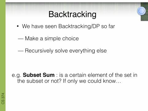
• We have seen Backtracking/DP so far
— Make a simple choice
— Recursively solve everything else
e.g. Subset Sum : is a certain element of the set in the subset or not? If only we could know…
Backtracking
CS
374
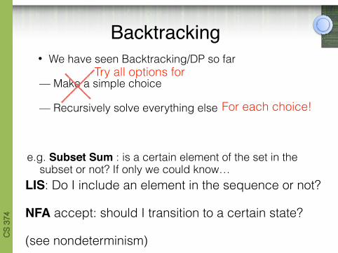
• We have seen Backtracking/DP so far
— Make a simple choice
— Recursively solve everything else
e.g. Subset Sum : is a certain element of the set in the subset or not? If only we could know…
Backtracking
Try all options for
For each choice!
LIS: Do I include an element in the sequence or not?
NFA accept: should I transition to a certain state?
(see nondeterminism)
CS
374
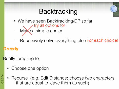
• We have seen Backtracking/DP so far
— Make a simple choice
— Recursively solve everything else
Backtracking
Try all options for
For each choice!
Greedy
Really tempting to
• Choose one option
• Recurse (e.g. Edit Distance: choose two characters that are equal to leave them as such)

CS
374
Course Policy on Greedy
• When you use greedy algorithm, you need to ALWAYS prove correctness. Otherwise you get a zero, EVEN IF THE ALGORITHM IS CORRECT!
• Greedy is a loaded gun!

CS
374
• Sorting files on magnetic tape (not RAM)
• Remember music cassettes?
• Blue Water Supercomputer.
Greedy Algorithm Example

CS
374
• Sorting files on magnetic tape (not RAM)
• Remember music cassettes?
• Blue Water Supercomputer.
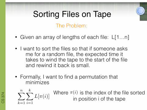
The Problem:
• Given an array of lengths of each file: L[1…n]
• I want to sort the files so that if someone asks me for a random file, the expected time it takes to wind the tape to the start of the file and rewind it back is small.
Greedy Algorithm Example
CS
374
The Problem:
• Given an array of lengths of each file: L[1…n]
• I want to sort the files so that if someone asks me for a random file, the expected time it takes to wind the tape to the start of the file and rewind it back is small.
• Formally, I want to find a permutation that minimizes
Sorting Files on Tape
nX
k=1
kX
i=1
L[⇡(i)]Where is the index of the file sorted
in position i of the tape ⇡(i)
CS
374
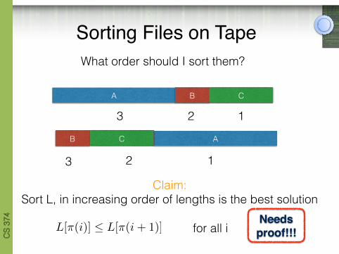
Sorting Files on Tape
A B C
What order should I sort them?
AB C
Claim: Sort L, in increasing order of lengths is the best solution
3 2 1
3 2 1
L[⇡(i)] L[⇡(i + 1)] for all iNeeds proof!!!
CS
374
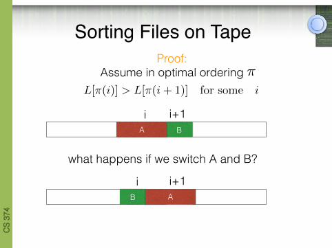
Sorting Files on TapeProof:
Assume in optimal ordering L[⇡(i)] > L[⇡(i + 1)] for some i
⇡
B
iA
i+1
B
iA
i+1
what happens if we switch A and B?
CS
374
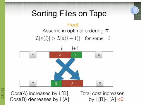
Sorting Files on TapeProof:
Assume in optimal ordering L[⇡(i)] > L[⇡(i + 1)] for some i
⇡
B
iA
i+1
B
iA
i+1X
X
Y
Y
Cost(A) increases by L[B] Cost(B) decreases by L[A]
Total cost increases by L[B]-L[A] <0

CS
374
Exchange Argument• Consider any non-greedy solution
• Perform an exchange to make the solution look more greedy
• Argue that the new solution after doing the exchange is no worse.
• In out example, the new solution was strictly better, so greedy is the only way.
CS
374
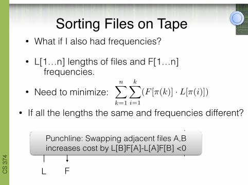
Sorting Files on Tape• What if I also had frequencies?
• L[1…n] lengths of files and F[1…n] frequencies.
• Need to minimize:nX
k=1
kX
i=1
(F [⇡(k)] · L[⇡(i)])
L F
If both are different? Sort by L/F (ratio!)
Punchline: Swapping adjacent files A,B increases cost by L[B]F[A]-L[A]F[B] <0
• If all the lengths the same and frequencies different?

CS
374
• University decides to start a new major, CS+ climbing
• Degree requirements involve taking certain number of classes, certain hours and certain categories.
• Bulk of the degree is determined by taking a certain number of classes. None of these classes require actual work.
• Without the instructors permission, you cannot register for two classes whose times overlap.
• You only need to sign up! Goal: sign up for as many classes as possible, without overlapping classes.
Class Scheduling

CS
374
• Given a collection of intervals with start and end time, want to choose a subset of those intervals such that no pair overlaps.
• Subset needs to be as large as possible.
• Model it as a graph problem (next time): Independent Set!
Class Scheduling
CS
374
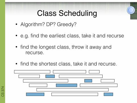
• Algorithm? DP? Greedy?
• e.g. find the earliest class, take it and recurse
• find the longest class, throw it away and recurse.
• find the shortest class, take it and recurse.
Class Scheduling
CS
374
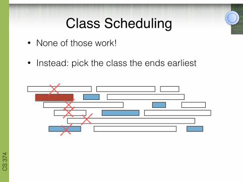
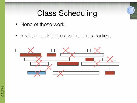
• None of those work!
• Instead: pick the class the ends earliest
Class Scheduling
CS
374
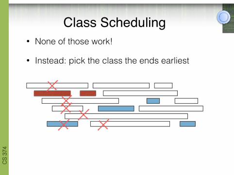
• None of those work!
• Instead: pick the class the ends earliest
Class Scheduling

CS
374
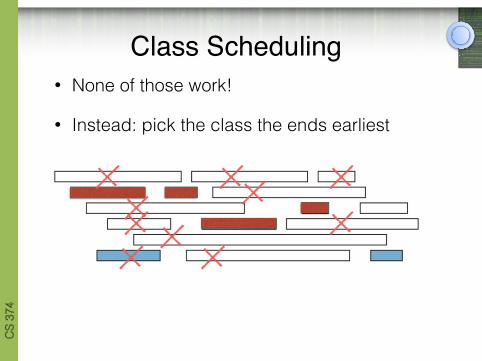
• None of those work!
• Instead: pick the class the ends earliest
Class Scheduling
CS
374
• None of those work!
• Instead: pick the class the ends earliest
Class Scheduling
CS
374
• None of those work!
• Instead: pick the class the ends earliest
Class Scheduling
CS
374
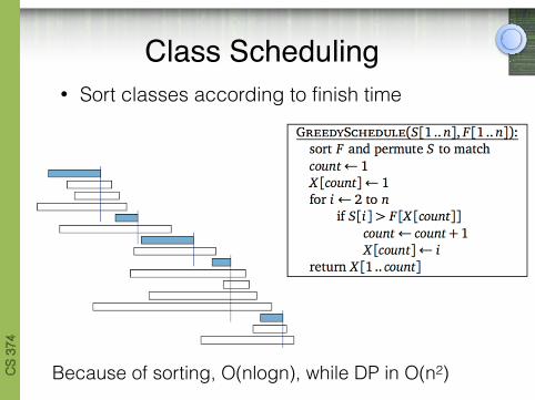
• Sort classes according to finish time
Class Scheduling
Because of sorting, O(nlogn), while DP in O(n2)
CS
374
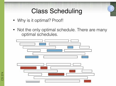
• Why is it optimal? Proof!
• Not the only optimal schedule. There are many optimal schedules.
Class Scheduling

CS
374
• Exchange argument.
• Think of it as a recursive algorithm. Pick the class what finishes first and then recurse.
• Proof by induction!
Class Scheduling
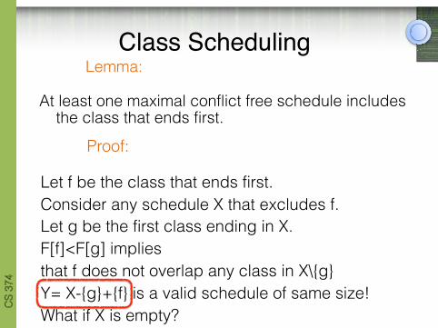
Lemma:
At least one maximal conflict free schedule includes the class that ends first.
CS
374
Lemma:
At least one maximal conflict free schedule includes the class that ends first.
Class Scheduling
Proof:
Let f be the class that ends first. Consider any schedule X that excludes f. Let g be the first class ending in X. F[f]<F[g] implies that f does not overlap any class in X\{g} Y= X-{g}+{f} is a valid schedule of same size! What if X is empty?

CS
374
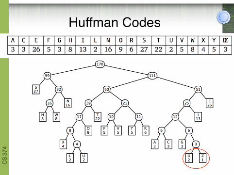
• Binary code assigns a string of 0s and 1s to each character in the alphabet.
• 7-bit ASCII code, Unicode, Morse
• We want the code to be prefix free (Morse code is not).
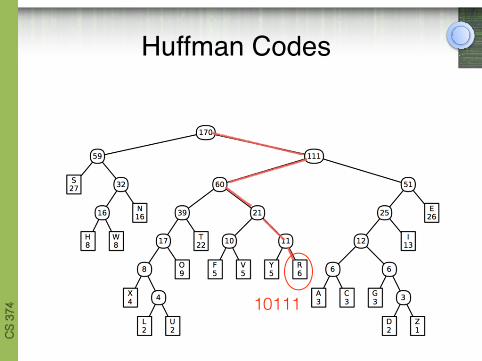
• Any prefix free code can be visualized as a binary code tree, where the characters are stored at the leafs.
• Codeword for each symbol is given by the path from the root to the corresponding leaf (e.g 1 for right 0 for left).
• Length of codeword for a symbol is the depth of the corresponding leaf.
Huffman Codes
CS
374
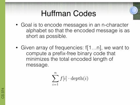
• Goal is to encode messages in an n-character alphabet so that the encoded message is as short as possible.
• Given array of frequencies: f[1…n], we want to compute a prefix-free binary code that minimizes the total encoded length of message.
Huffman Codes
nX
i=1
f [i] · depth(i)
CS
374
Huffman Codes
10111
CS
374
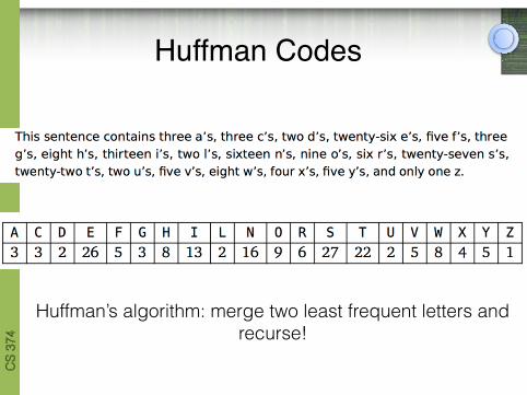
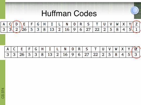
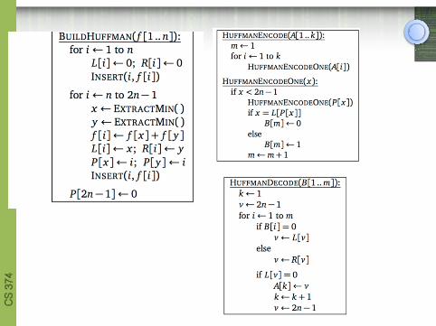
Huffman Codes
Huffman’s algorithm: merge two least frequent letters and recurse!
CS
374
Huffman Codes
CS
374
Huffman Codes
CS
374
Lemma: Let x and y be the two least frequent characters. There is an optimal code tree in which x and y are siblings, and have the largest depth of any leaf.
Huffman Codes
Proof: Exchange argument!
Assume, for the optimal schedule that the deepest two leaves are not x and y.
CS
374

Part I
Greedy Algorithms: Tools andTechniques
Chandra & Manoj (UIUC) CS374 2 Fall 2015 2 / 40

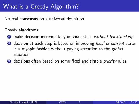
What is a Greedy Algorithm?
No real consensus on a universal definition.
Greedy algorithms:
1 make decision incrementally in small steps without backtracking
2 decision at each step is based on improving local or current statein a myopic fashion without paying attention to the globalsituation
3 decisions often based on some fixed and simple priority rules
Chandra & Manoj (UIUC) CS374 3 Fall 2015 3 / 40

Pros and Cons of Greedy Algorithms
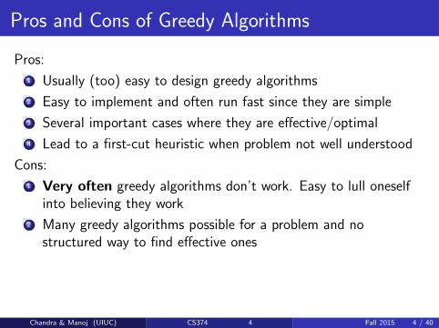
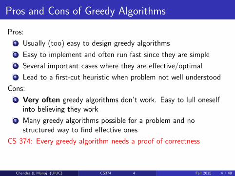
Pros:
1 Usually (too) easy to design greedy algorithms
2 Easy to implement and often run fast since they are simple
3 Several important cases where they are effective/optimal
4 Lead to a first-cut heuristic when problem not well understood
Cons:
1 Very often greedy algorithms don’t work. Easy to lull oneselfinto believing they work
2 Many greedy algorithms possible for a problem and nostructured way to find effective ones
CS 374: Every greedy algorithm needs a proof of correctness
Chandra & Manoj (UIUC) CS374 4 Fall 2015 4 / 40
Pros and Cons of Greedy Algorithms
Pros:
1 Usually (too) easy to design greedy algorithms
2 Easy to implement and often run fast since they are simple
3 Several important cases where they are effective/optimal
4 Lead to a first-cut heuristic when problem not well understood
Cons:
1 Very often greedy algorithms don’t work. Easy to lull oneselfinto believing they work
2 Many greedy algorithms possible for a problem and nostructured way to find effective ones
CS 374: Every greedy algorithm needs a proof of correctness
Chandra & Manoj (UIUC) CS374 4 Fall 2015 4 / 40
Greedy Algorithm Types
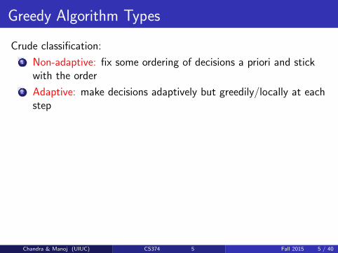
Crude classification:
1 Non-adaptive: fix some ordering of decisions a priori and stickwith the order
2 Adaptive: make decisions adaptively but greedily/locally at eachstep
Plan:
1 See several examples
2 Pick up some proof techniques
Chandra & Manoj (UIUC) CS374 5 Fall 2015 5 / 40

Greedy Algorithm Types
Crude classification:
1 Non-adaptive: fix some ordering of decisions a priori and stickwith the order
2 Adaptive: make decisions adaptively but greedily/locally at eachstep
Plan:
1 See several examples
2 Pick up some proof techniques
Chandra & Manoj (UIUC) CS374 5 Fall 2015 5 / 40

Part II
Scheduling Jobs to Minimize AverageWaiting Time
Chandra & Manoj (UIUC) CS374 6 Fall 2015 6 / 40

The Problem
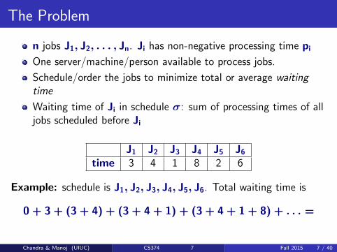
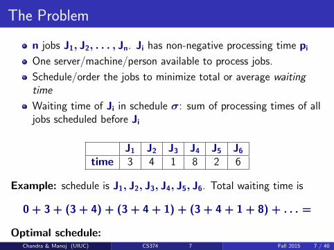
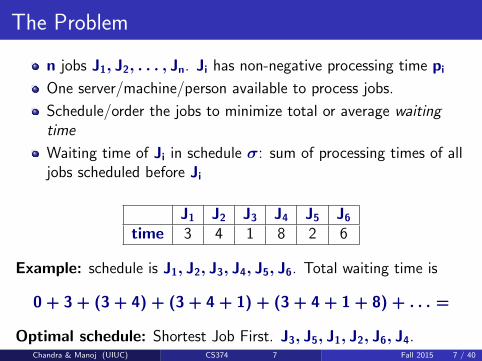
n jobs J1, J2, . . . , Jn. Ji has non-negative processing time pi
One server/machine/person available to process jobs.
Schedule/order the jobs to minimize total or average waitingtime
Waiting time of Ji in schedule σ: sum of processing times of alljobs scheduled before Ji
J1 J2 J3 J4 J5 J6time 3 4 1 8 2 6
Example: schedule is J1, J2, J3, J4, J5, J6. Total waiting time is
0 + 3 + (3 + 4) + (3 + 4 + 1) + (3 + 4 + 1 + 8) + . . . =
Optimal schedule: Shortest Job First. J3, J5, J1, J2, J6, J4.
Chandra & Manoj (UIUC) CS374 7 Fall 2015 7 / 40
The Problem
n jobs J1, J2, . . . , Jn. Ji has non-negative processing time pi
One server/machine/person available to process jobs.
Schedule/order the jobs to minimize total or average waitingtime
Waiting time of Ji in schedule σ: sum of processing times of alljobs scheduled before Ji
J1 J2 J3 J4 J5 J6time 3 4 1 8 2 6
Example: schedule is J1, J2, J3, J4, J5, J6. Total waiting time is
0 + 3 + (3 + 4) + (3 + 4 + 1) + (3 + 4 + 1 + 8) + . . . =
Optimal schedule:
Shortest Job First. J3, J5, J1, J2, J6, J4.
Chandra & Manoj (UIUC) CS374 7 Fall 2015 7 / 40
The Problem
n jobs J1, J2, . . . , Jn. Ji has non-negative processing time pi
One server/machine/person available to process jobs.
Schedule/order the jobs to minimize total or average waitingtime
Waiting time of Ji in schedule σ: sum of processing times of alljobs scheduled before Ji
J1 J2 J3 J4 J5 J6time 3 4 1 8 2 6
Example: schedule is J1, J2, J3, J4, J5, J6. Total waiting time is
0 + 3 + (3 + 4) + (3 + 4 + 1) + (3 + 4 + 1 + 8) + . . . =
Optimal schedule: Shortest Job First. J3, J5, J1, J2, J6, J4.Chandra & Manoj (UIUC) CS374 7 Fall 2015 7 / 40
Optimality of SJF
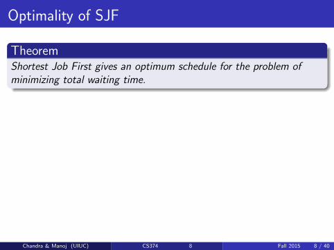
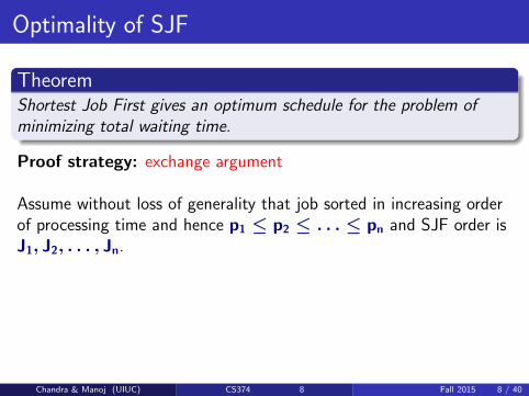
TheoremShortest Job First gives an optimum schedule for the problem ofminimizing total waiting time.
Proof strategy: exchange argument
Assume without loss of generality that job sorted in increasing orderof processing time and hence p1 ≤ p2 ≤ . . . ≤ pn and SJF order isJ1, J2, . . . , Jn.
Chandra & Manoj (UIUC) CS374 8 Fall 2015 8 / 40

Optimality of SJF
TheoremShortest Job First gives an optimum schedule for the problem ofminimizing total waiting time.
Proof strategy: exchange argument
Assume without loss of generality that job sorted in increasing orderof processing time and hence p1 ≤ p2 ≤ . . . ≤ pn and SJF order isJ1, J2, . . . , Jn.
Chandra & Manoj (UIUC) CS374 8 Fall 2015 8 / 40
Inversions
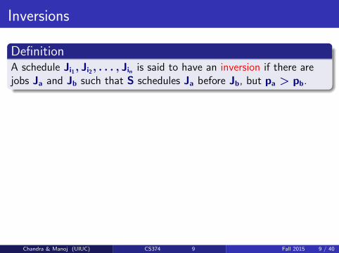
DefinitionA schedule Ji1, Ji2, . . . , Jin is said to have an inversion if there arejobs Ja and Jb such that S schedules Ja before Jb, but pa > pb.
ClaimIf a schedule has an inversion then there is an inversion between twoadjacently scheduled jobs.
Proof: exercise.
Chandra & Manoj (UIUC) CS374 9 Fall 2015 9 / 40
Inversions
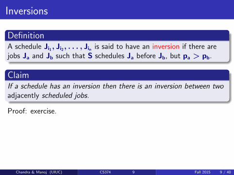
DefinitionA schedule Ji1, Ji2, . . . , Jin is said to have an inversion if there arejobs Ja and Jb such that S schedules Ja before Jb, but pa > pb.
ClaimIf a schedule has an inversion then there is an inversion between twoadjacently scheduled jobs.
Proof: exercise.
Chandra & Manoj (UIUC) CS374 9 Fall 2015 9 / 40
Proof of optimality of SJF
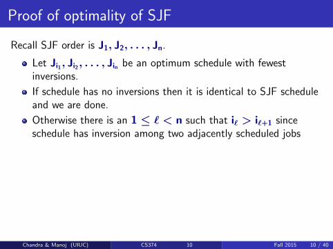
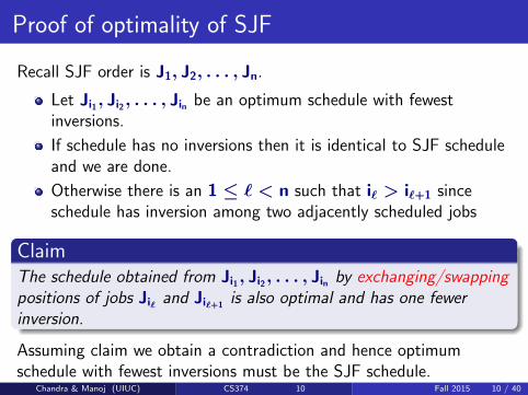
Recall SJF order is J1, J2, . . . , Jn.
Let Ji1, Ji2, . . . , Jin be an optimum schedule with fewestinversions.
If schedule has no inversions then it is identical to SJF scheduleand we are done.
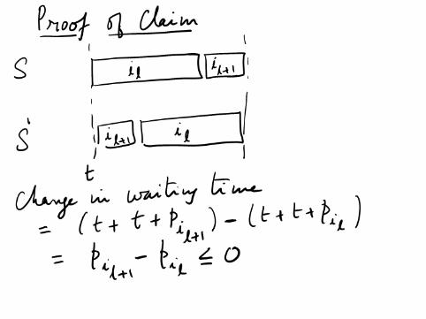
Otherwise there is an 1 ≤ ` < n such that i` > i`+1 sinceschedule has inversion among two adjacently scheduled jobs
ClaimThe schedule obtained from Ji1, Ji2, . . . , Jin by exchanging/swappingpositions of jobs Ji` and Ji`+1
is also optimal and has one fewerinversion.
Assuming claim we obtain a contradiction and hence optimumschedule with fewest inversions must be the SJF schedule.
Chandra & Manoj (UIUC) CS374 10 Fall 2015 10 / 40
Proof of optimality of SJF
Recall SJF order is J1, J2, . . . , Jn.
Let Ji1, Ji2, . . . , Jin be an optimum schedule with fewestinversions.
If schedule has no inversions then it is identical to SJF scheduleand we are done.
Otherwise there is an 1 ≤ ` < n such that i` > i`+1 sinceschedule has inversion among two adjacently scheduled jobs
ClaimThe schedule obtained from Ji1, Ji2, . . . , Jin by exchanging/swappingpositions of jobs Ji` and Ji`+1
is also optimal and has one fewerinversion.
Assuming claim we obtain a contradiction and hence optimumschedule with fewest inversions must be the SJF schedule.
Chandra & Manoj (UIUC) CS374 10 Fall 2015 10 / 40
Part III
Scheduling to Minimize Lateness
Chandra & Manoj (UIUC) CS374 11 Fall 2015 11 / 40
Scheduling to Minimize Lateness
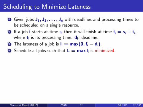
1 Given jobs J1, J2, . . . , Jn with deadlines and processing times tobe scheduled on a single resource.
2 If a job i starts at time si then it will finish at time fi = si + ti,where ti is its processing time. di: deadline.
3 The lateness of a job is li = max(0, fi − di).4 Schedule all jobs such that L = max li is minimized.
J1 J2 J3 J4 J5 J6ti 3 2 1 4 3 2di 6 8 9 9 14 15
0 1 2 3 4 5 6 7 8 9 10 11 12 13 14 15
J3 J2 J6 J1 J5 J4
l1 = 2 l5 = 0 l4 = 6
Chandra & Manoj (UIUC) CS374 12 Fall 2015 12 / 40

Scheduling to Minimize Lateness
1 Given jobs J1, J2, . . . , Jn with deadlines and processing times tobe scheduled on a single resource.
2 If a job i starts at time si then it will finish at time fi = si + ti,where ti is its processing time. di: deadline.
3 The lateness of a job is li = max(0, fi − di).4 Schedule all jobs such that L = max li is minimized.
J1 J2 J3 J4 J5 J6ti 3 2 1 4 3 2di 6 8 9 9 14 15
0 1 2 3 4 5 6 7 8 9 10 11 12 13 14 15
J3 J2 J6 J1 J5 J4
l1 = 2 l5 = 0 l4 = 6
Chandra & Manoj (UIUC) CS374 12 Fall 2015 12 / 40

Greedy Template
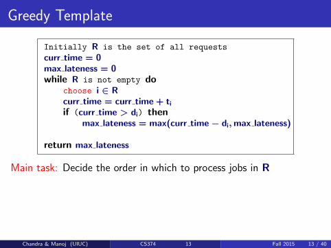
Initially R is the set of all requests
curr time = 0max lateness = 0while R is not empty do
choose i ∈ Rcurr time = curr time + tiif (curr time > di) then
max lateness = max(curr time− di,max lateness)
return max lateness
Main task: Decide the order in which to process jobs in R
Chandra & Manoj (UIUC) CS374 13 Fall 2015 13 / 40
Greedy Template
Initially R is the set of all requests
curr time = 0max lateness = 0while R is not empty do
choose i ∈ Rcurr time = curr time + tiif (curr time > di) then
max lateness = max(curr time− di,max lateness)
return max lateness
Main task: Decide the order in which to process jobs in R
Chandra & Manoj (UIUC) CS374 13 Fall 2015 13 / 40
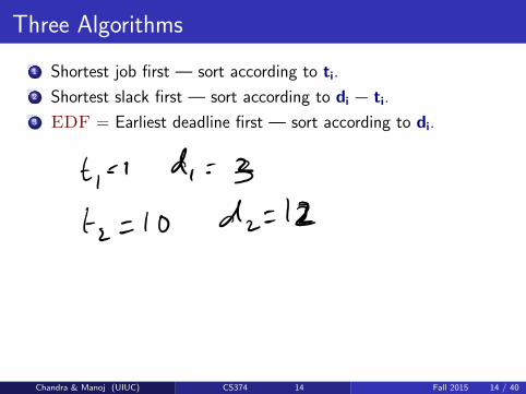
Three Algorithms
1 Shortest job first — sort according to ti.
2 Shortest slack first — sort according to di − ti.
3 EDF = Earliest deadline first — sort according to di.
Counter examples for first two: exercise
Chandra & Manoj (UIUC) CS374 14 Fall 2015 14 / 40
Three Algorithms
1 Shortest job first — sort according to ti.
2 Shortest slack first — sort according to di − ti.
3 EDF = Earliest deadline first — sort according to di.
Counter examples for first two: exercise
Chandra & Manoj (UIUC) CS374 14 Fall 2015 14 / 40
Earliest Deadline First
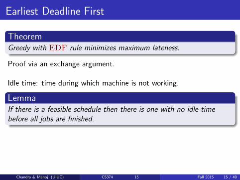
TheoremGreedy with EDF rule minimizes maximum lateness.
Proof via an exchange argument.
Idle time: time during which machine is not working.
LemmaIf there is a feasible schedule then there is one with no idle timebefore all jobs are finished.
Chandra & Manoj (UIUC) CS374 15 Fall 2015 15 / 40
Earliest Deadline First
TheoremGreedy with EDF rule minimizes maximum lateness.
Proof via an exchange argument.
Idle time: time during which machine is not working.
LemmaIf there is a feasible schedule then there is one with no idle timebefore all jobs are finished.
Chandra & Manoj (UIUC) CS374 15 Fall 2015 15 / 40
Inversions
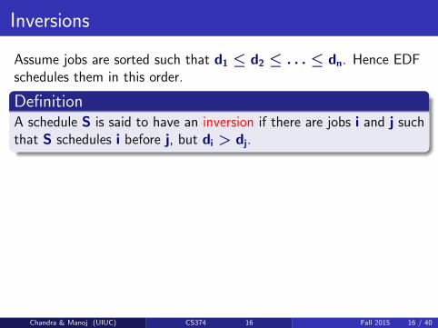
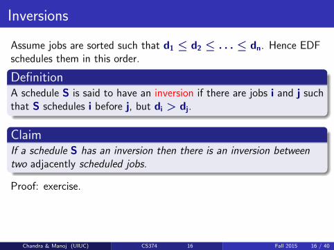
Assume jobs are sorted such that d1 ≤ d2 ≤ . . . ≤ dn. Hence EDFschedules them in this order.
DefinitionA schedule S is said to have an inversion if there are jobs i and j suchthat S schedules i before j, but di > dj.
ClaimIf a schedule S has an inversion then there is an inversion betweentwo adjacently scheduled jobs.
Proof: exercise.
Chandra & Manoj (UIUC) CS374 16 Fall 2015 16 / 40
Inversions
Assume jobs are sorted such that d1 ≤ d2 ≤ . . . ≤ dn. Hence EDFschedules them in this order.
DefinitionA schedule S is said to have an inversion if there are jobs i and j suchthat S schedules i before j, but di > dj.
ClaimIf a schedule S has an inversion then there is an inversion betweentwo adjacently scheduled jobs.
Proof: exercise.
Chandra & Manoj (UIUC) CS374 16 Fall 2015 16 / 40
Proof sketch of Optimality of EDP
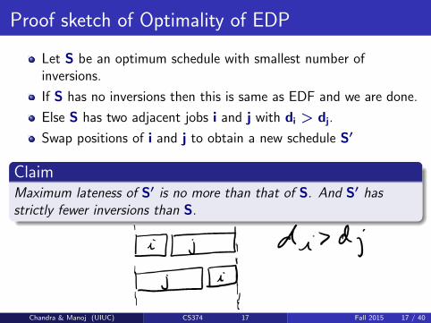
Let S be an optimum schedule with smallest number ofinversions.
If S has no inversions then this is same as EDF and we are done.
Else S has two adjacent jobs i and j with di > dj.
Swap positions of i and j to obtain a new schedule S′
ClaimMaximum lateness of S′ is no more than that of S. And S′ hasstrictly fewer inversions than S.
Chandra & Manoj (UIUC) CS374 17 Fall 2015 17 / 40
Part IV
Maximum Weight Subset of Elements:Cardinality and Beyond
Chandra & Manoj (UIUC) CS374 18 Fall 2015 18 / 40
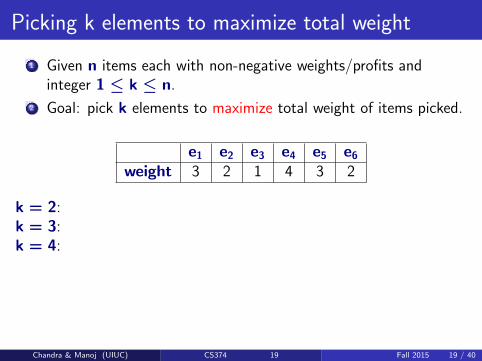
Picking k elements to maximize total weight
1 Given n items each with non-negative weights/profits andinteger 1 ≤ k ≤ n.
2 Goal: pick k elements to maximize total weight of items picked.
e1 e2 e3 e4 e5 e6weight 3 2 1 4 3 2
k = 2:k = 3:k = 4:
Chandra & Manoj (UIUC) CS374 19 Fall 2015 19 / 40

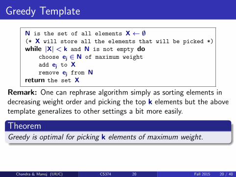
Greedy Template
N is the set of all elements X← ∅(* X will store all the elements that will be picked *)
while |X| < k and N is not empty dochoose ej ∈ N of maximum weight
add ej to Xremove ej from N
return the set X
Remark: One can rephrase algorithm simply as sorting elements indecreasing weight order and picking the top k elements but the abovetemplate generalizes to other settings a bit more easily.
TheoremGreedy is optimal for picking k elements of maximum weight.
Chandra & Manoj (UIUC) CS374 20 Fall 2015 20 / 40
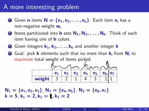
A more interesting problem
1 Given n items N = {e1, e2, . . . , en}. Each item ei has anon-negative weight wi.
2 Items partitioned into h sets N1,N2, . . . ,Nh. Think of eachitem having one of h colors.
3 Given integers k1, k2, . . . , kh and another integer k
4 Goal: pick k elements such that no more than ki from Ni tomaximize total weight of items picked.
e1 e2 e3 e4 e5 e6, e7weight 3 2 1 4 3 2, 1
N1 = {e1, e2, e3}, N2 = {e4, e5}, N3 = {e6, e7}k = 5, k1 = 2, k2 = 2, k3 = 2
Chandra & Manoj (UIUC) CS374 21 Fall 2015 21 / 40
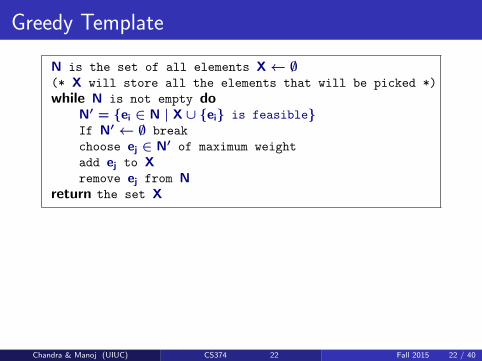
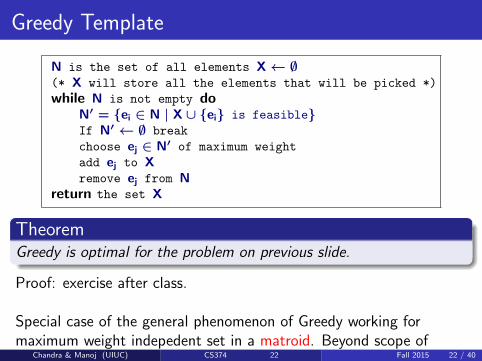
Greedy Template
N is the set of all elements X← ∅(* X will store all the elements that will be picked *)
while N is not empty doN′ = {ei ∈ N | X ∪ {ei} is feasible}If N′ ← ∅ break
choose ej ∈ N′ of maximum weight
add ej to Xremove ej from N
return the set X
TheoremGreedy is optimal for the problem on previous slide.
Proof: exercise after class.
Special case of the general phenomenon of Greedy working formaximum weight indepedent set in a matroid. Beyond scope ofcourse.
Chandra & Manoj (UIUC) CS374 22 Fall 2015 22 / 40
Greedy Template
N is the set of all elements X← ∅(* X will store all the elements that will be picked *)
while N is not empty doN′ = {ei ∈ N | X ∪ {ei} is feasible}If N′ ← ∅ break
choose ej ∈ N′ of maximum weight
add ej to Xremove ej from N
return the set X
TheoremGreedy is optimal for the problem on previous slide.
Proof: exercise after class.
Special case of the general phenomenon of Greedy working formaximum weight indepedent set in a matroid. Beyond scope ofcourse.Chandra & Manoj (UIUC) CS374 22 Fall 2015 22 / 40
Part V
Interval Scheduling
Chandra & Manoj (UIUC) CS374 23 Fall 2015 23 / 40
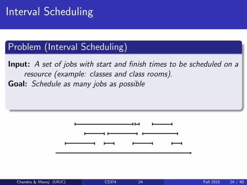
Interval Scheduling
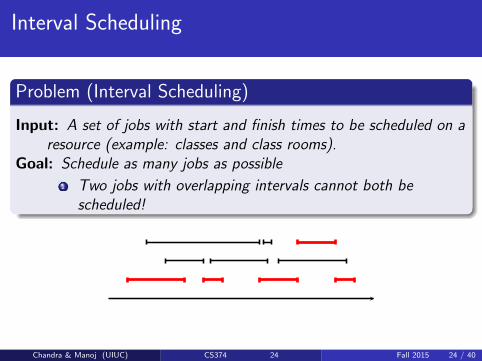
Problem (Interval Scheduling)
Input: A set of jobs with start and finish times to be scheduled on aresource (example: classes and class rooms).
Goal: Schedule as many jobs as possible
1 Two jobs with overlapping intervals cannot both bescheduled!
Chandra & Manoj (UIUC) CS374 24 Fall 2015 24 / 40
Interval Scheduling
Problem (Interval Scheduling)
Input: A set of jobs with start and finish times to be scheduled on aresource (example: classes and class rooms).
Goal: Schedule as many jobs as possible
1 Two jobs with overlapping intervals cannot both bescheduled!
Chandra & Manoj (UIUC) CS374 24 Fall 2015 24 / 40
Greedy Template
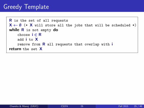
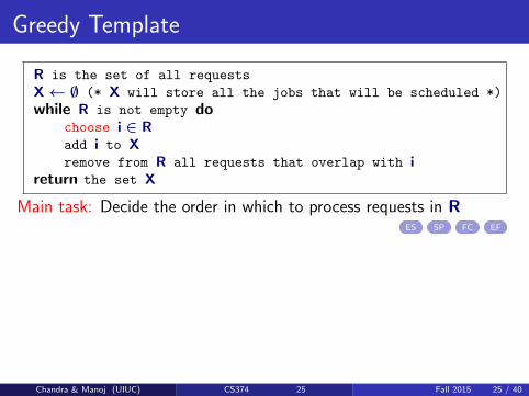
R is the set of all requests
X← ∅ (* X will store all the jobs that will be scheduled *)
while R is not empty dochoose i ∈ Radd i to Xremove from R all requests that overlap with i
return the set X
Main task: Decide the order in which to process requests in RES SP FC EF
Chandra & Manoj (UIUC) CS374 25 Fall 2015 25 / 40
Greedy Template
R is the set of all requests
X← ∅ (* X will store all the jobs that will be scheduled *)
while R is not empty dochoose i ∈ Radd i to Xremove from R all requests that overlap with i
return the set X
Main task: Decide the order in which to process requests in RES SP FC EF
Chandra & Manoj (UIUC) CS374 25 Fall 2015 25 / 40
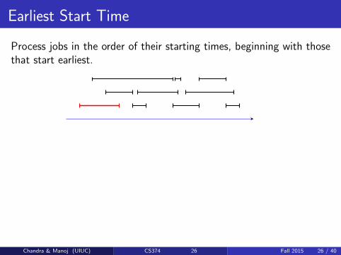
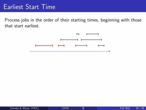
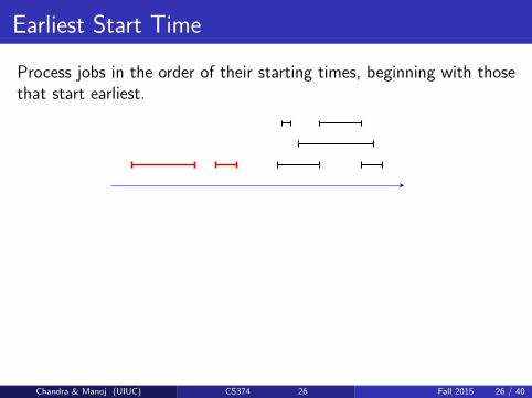
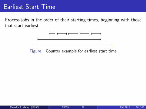
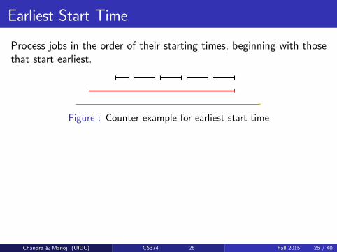
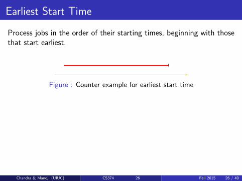
Earliest Start Time
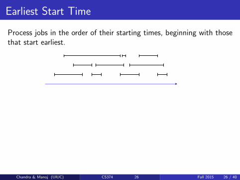
Process jobs in the order of their starting times, beginning with thosethat start earliest.
Chandra & Manoj (UIUC) CS374 26 Fall 2015 26 / 40
Earliest Start Time
Process jobs in the order of their starting times, beginning with thosethat start earliest.
Chandra & Manoj (UIUC) CS374 26 Fall 2015 26 / 40

Earliest Start Time
Process jobs in the order of their starting times, beginning with thosethat start earliest.
Chandra & Manoj (UIUC) CS374 26 Fall 2015 26 / 40
Earliest Start Time
Process jobs in the order of their starting times, beginning with thosethat start earliest.
Chandra & Manoj (UIUC) CS374 26 Fall 2015 26 / 40
Earliest Start Time
Process jobs in the order of their starting times, beginning with thosethat start earliest.
Chandra & Manoj (UIUC) CS374 26 Fall 2015 26 / 40
Earliest Start Time
Process jobs in the order of their starting times, beginning with thosethat start earliest.
Chandra & Manoj (UIUC) CS374 26 Fall 2015 26 / 40
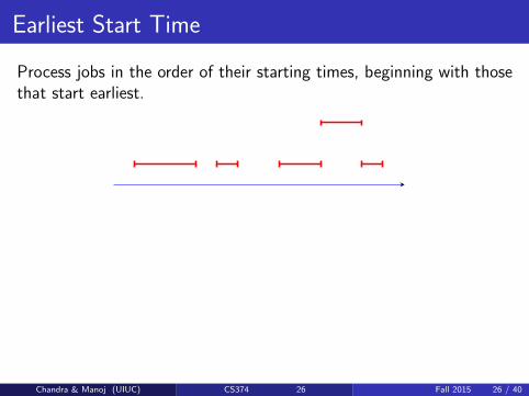
Earliest Start Time
Process jobs in the order of their starting times, beginning with thosethat start earliest.
Figure : Counter example for earliest start time
Chandra & Manoj (UIUC) CS374 26 Fall 2015 26 / 40
Earliest Start Time
Process jobs in the order of their starting times, beginning with thosethat start earliest.
Figure : Counter example for earliest start time
Chandra & Manoj (UIUC) CS374 26 Fall 2015 26 / 40
Earliest Start Time
Process jobs in the order of their starting times, beginning with thosethat start earliest.
Figure : Counter example for earliest start time
Chandra & Manoj (UIUC) CS374 26 Fall 2015 26 / 40
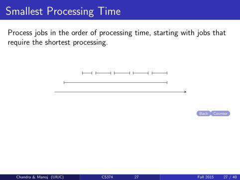
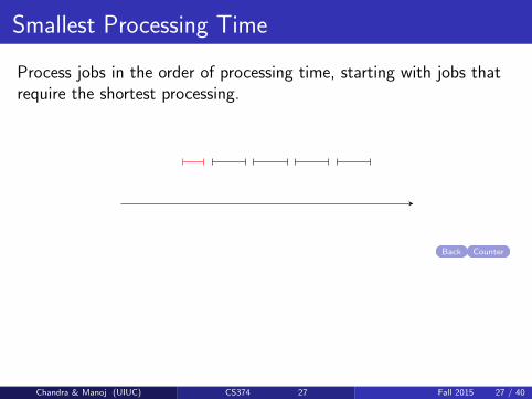
Smallest Processing Time
Process jobs in the order of processing time, starting with jobs thatrequire the shortest processing.
Back Counter
Chandra & Manoj (UIUC) CS374 27 Fall 2015 27 / 40

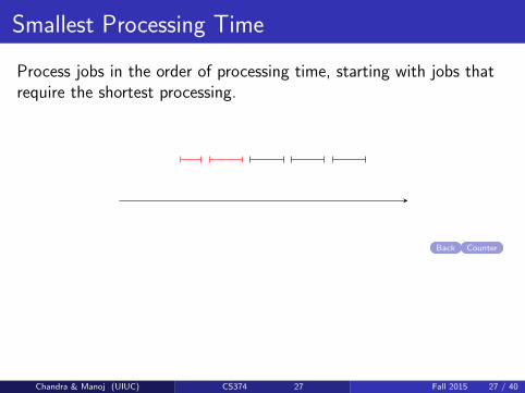
Smallest Processing Time
Process jobs in the order of processing time, starting with jobs thatrequire the shortest processing.
Back Counter
Chandra & Manoj (UIUC) CS374 27 Fall 2015 27 / 40
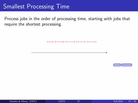
Smallest Processing Time
Process jobs in the order of processing time, starting with jobs thatrequire the shortest processing.
Back Counter
Chandra & Manoj (UIUC) CS374 27 Fall 2015 27 / 40
Smallest Processing Time
Process jobs in the order of processing time, starting with jobs thatrequire the shortest processing.
Back Counter
Chandra & Manoj (UIUC) CS374 27 Fall 2015 27 / 40
Smallest Processing Time
Process jobs in the order of processing time, starting with jobs thatrequire the shortest processing.
Back Counter
Chandra & Manoj (UIUC) CS374 27 Fall 2015 27 / 40
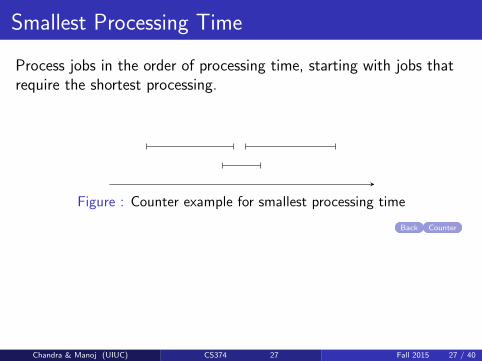
Smallest Processing Time
Process jobs in the order of processing time, starting with jobs thatrequire the shortest processing.
Figure : Counter example for smallest processing time
Back Counter
Chandra & Manoj (UIUC) CS374 27 Fall 2015 27 / 40

Smallest Processing Time
Process jobs in the order of processing time, starting with jobs thatrequire the shortest processing.
Figure : Counter example for smallest processing time
Back Counter
Chandra & Manoj (UIUC) CS374 27 Fall 2015 27 / 40
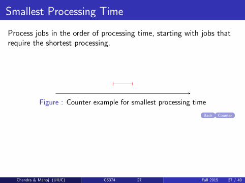
Smallest Processing Time
Process jobs in the order of processing time, starting with jobs thatrequire the shortest processing.
Figure : Counter example for smallest processing time
Back Counter
Chandra & Manoj (UIUC) CS374 27 Fall 2015 27 / 40

Fewest Conflicts
Process jobs in that have the fewest “conflicts” first.
Back Counter
Chandra & Manoj (UIUC) CS374 28 Fall 2015 28 / 40

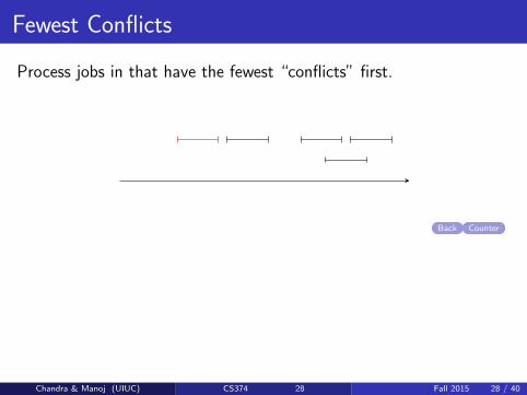
Fewest Conflicts
Process jobs in that have the fewest “conflicts” first.
Back Counter
Chandra & Manoj (UIUC) CS374 28 Fall 2015 28 / 40
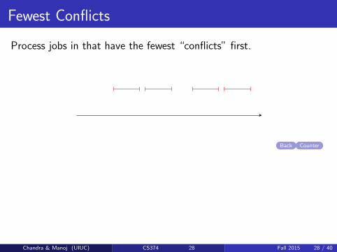
Fewest Conflicts
Process jobs in that have the fewest “conflicts” first.
Back Counter
Chandra & Manoj (UIUC) CS374 28 Fall 2015 28 / 40

Fewest Conflicts
Process jobs in that have the fewest “conflicts” first.
Back Counter
Chandra & Manoj (UIUC) CS374 28 Fall 2015 28 / 40
Fewest Conflicts
Process jobs in that have the fewest “conflicts” first.
Back Counter
Chandra & Manoj (UIUC) CS374 28 Fall 2015 28 / 40

Fewest Conflicts
Process jobs in that have the fewest “conflicts” first.
Figure : Counter example for fewest conflicts
Back Counter
Chandra & Manoj (UIUC) CS374 28 Fall 2015 28 / 40

Fewest Conflicts
Process jobs in that have the fewest “conflicts” first.
Figure : Counter example for fewest conflicts
Back Counter
Chandra & Manoj (UIUC) CS374 28 Fall 2015 28 / 40
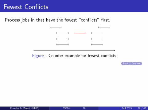
Fewest Conflicts
Process jobs in that have the fewest “conflicts” first.
Figure : Counter example for fewest conflicts
Back Counter
Chandra & Manoj (UIUC) CS374 28 Fall 2015 28 / 40

Fewest Conflicts
Process jobs in that have the fewest “conflicts” first.
Figure : Counter example for fewest conflicts
Back Counter
Chandra & Manoj (UIUC) CS374 28 Fall 2015 28 / 40

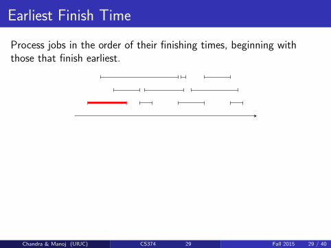
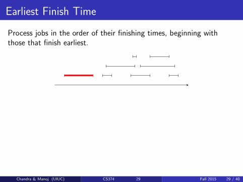
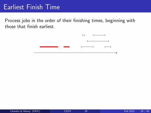
Earliest Finish Time
Process jobs in the order of their finishing times, beginning withthose that finish earliest.
Chandra & Manoj (UIUC) CS374 29 Fall 2015 29 / 40
Earliest Finish Time
Process jobs in the order of their finishing times, beginning withthose that finish earliest.
Chandra & Manoj (UIUC) CS374 29 Fall 2015 29 / 40
Earliest Finish Time
Process jobs in the order of their finishing times, beginning withthose that finish earliest.
Chandra & Manoj (UIUC) CS374 29 Fall 2015 29 / 40

Earliest Finish Time
Process jobs in the order of their finishing times, beginning withthose that finish earliest.
Chandra & Manoj (UIUC) CS374 29 Fall 2015 29 / 40
Earliest Finish Time
Process jobs in the order of their finishing times, beginning withthose that finish earliest.
Chandra & Manoj (UIUC) CS374 29 Fall 2015 29 / 40

Earliest Finish Time
Process jobs in the order of their finishing times, beginning withthose that finish earliest.
Chandra & Manoj (UIUC) CS374 29 Fall 2015 29 / 40

Earliest Finish Time
Process jobs in the order of their finishing times, beginning withthose that finish earliest.
Chandra & Manoj (UIUC) CS374 29 Fall 2015 29 / 40
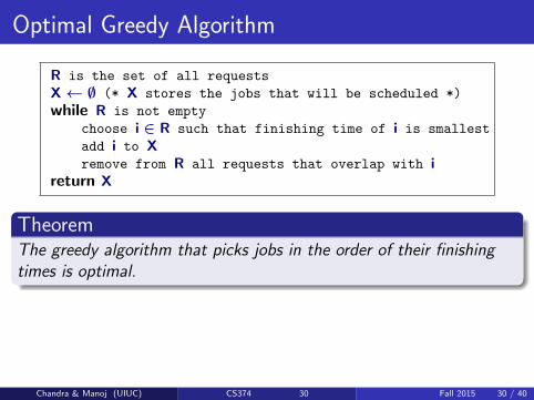
Optimal Greedy Algorithm
R is the set of all requests
X← ∅ (* X stores the jobs that will be scheduled *)
while R is not empty
choose i ∈ R such that finishing time of i is smallest
add i to Xremove from R all requests that overlap with i
return X
TheoremThe greedy algorithm that picks jobs in the order of their finishingtimes is optimal.
Chandra & Manoj (UIUC) CS374 30 Fall 2015 30 / 40
Proving Optimality
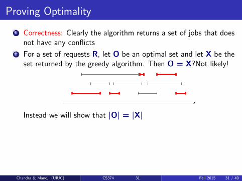
1 Correctness: Clearly the algorithm returns a set of jobs that doesnot have any conflicts
2 For a set of requests R, let O be an optimal set and let X be theset returned by the greedy algorithm. Then O = X?
Not likely!
Instead we will show that |O| = |X|
Chandra & Manoj (UIUC) CS374 31 Fall 2015 31 / 40
Proving Optimality
1 Correctness: Clearly the algorithm returns a set of jobs that doesnot have any conflicts
2 For a set of requests R, let O be an optimal set and let X be theset returned by the greedy algorithm. Then O = X?
Not likely!
Instead we will show that |O| = |X|
Chandra & Manoj (UIUC) CS374 31 Fall 2015 31 / 40
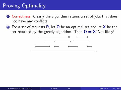
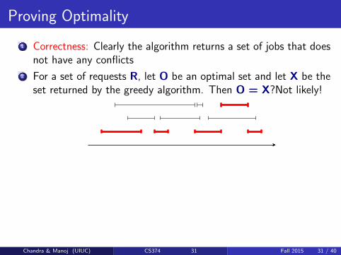
Proving Optimality
1 Correctness: Clearly the algorithm returns a set of jobs that doesnot have any conflicts
2 For a set of requests R, let O be an optimal set and let X be theset returned by the greedy algorithm. Then O = X?Not likely!
Instead we will show that |O| = |X|
Chandra & Manoj (UIUC) CS374 31 Fall 2015 31 / 40
Proof of Optimality: Key Lemma
LemmaLet i1 be first interval picked by Greedy. There exists an optimumsolution that contains i1.
Proof.Let O be an arbitrary optimum solution. If i1 ∈ O we are done.
Claim: If i1 6∈ O then there is exactly one interval j1 ∈ O thatconflicts with i1. (proof later)
1 Form a new set O′ by removing j1 from O and adding i1, that isO′ = (O− {j1}) ∪ {i1}.
2 From claim, O′ is a feasible solution (no conflicts).
3 Since |O′| = |O|, O′ is also an optimum solution and itcontains i1.
Chandra & Manoj (UIUC) CS374 32 Fall 2015 32 / 40
Proof of Optimality: Key Lemma
LemmaLet i1 be first interval picked by Greedy. There exists an optimumsolution that contains i1.
Proof.Let O be an arbitrary optimum solution. If i1 ∈ O we are done.Claim: If i1 6∈ O then there is exactly one interval j1 ∈ O thatconflicts with i1. (proof later)
1 Form a new set O′ by removing j1 from O and adding i1, that isO′ = (O− {j1}) ∪ {i1}.
2 From claim, O′ is a feasible solution (no conflicts).
3 Since |O′| = |O|, O′ is also an optimum solution and itcontains i1.
Chandra & Manoj (UIUC) CS374 32 Fall 2015 32 / 40
Proof of Claim
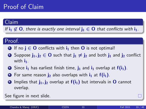
ClaimIf i1 6∈ O, there is exactly one interval j1 ∈ O that conflicts with i1.
Proof.1 If no j ∈ O conflicts with i1 then O is not optimal!
2 Suppose j1, j2 ∈ O such that j1 6= j2 and both j1 and j2 conflictwith i1.
3 Since i1 has earliest finish time, j1 and i1 overlap at f(i1).
4 For same reason j2 also overlaps with i1 at f(i1).
5 Implies that j1, j2 overlap at f(i1) but intervals in O cannotoverlap.
See figure in next slide.
Chandra & Manoj (UIUC) CS374 33 Fall 2015 33 / 40
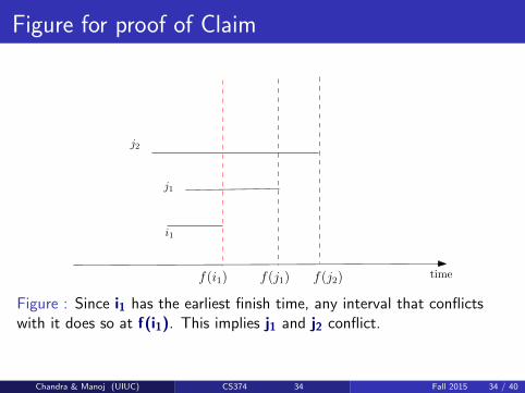
Figure for proof of Claim
f(i1) f(j1)
i1
j1
j2
f(j2) time
Figure : Since i1 has the earliest finish time, any interval that conflictswith it does so at f(i1). This implies j1 and j2 conflict.
Chandra & Manoj (UIUC) CS374 34 Fall 2015 34 / 40

Proof of Optimality of Earliest Finish Time First
Proof by Induction on number of intervals.Base Case: n = 1. Trivial since Greedy picks one interval.Induction Step: Assume theorem holds for i < n.Let I be an instance with n intervalsI′: I with i1 and all intervals that overlap with i1 removedG(I),G(I′): Solution produced by Greedy on I and I′
From Lemma, there is an optimum solution O to I and i1 ∈ O.Let O′ = O− {i1}. O′ is a solution to I′.
|G(I)| = 1 + |G(I′)| (from Greedy description)
≥ 1 + |O′| (By induction, G(I′) is optimum for I′)
= |O|
Chandra & Manoj (UIUC) CS374 35 Fall 2015 35 / 40
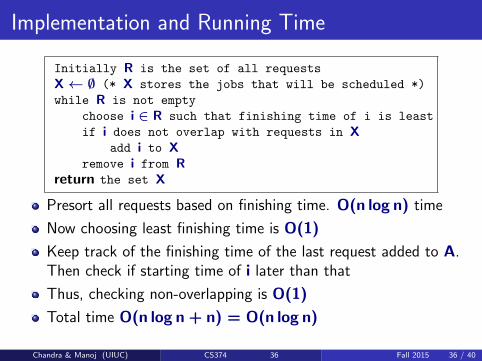
Implementation and Running Time
Initially R is the set of all requests
X← ∅ (* X stores the jobs that will be scheduled *)
while R is not empty
choose i ∈ R such that finishing time of i is least
if i does not overlap with requests in Xadd i to X
remove i from Rreturn the set X
Presort all requests based on finishing time. O(n log n) time
Now choosing least finishing time is O(1)
Keep track of the finishing time of the last request added to A.Then check if starting time of i later than that
Thus, checking non-overlapping is O(1)
Total time O(n log n + n) = O(n log n)
Chandra & Manoj (UIUC) CS374 36 Fall 2015 36 / 40

Comments
1 Interesting Exercise: smallest interval first picks at least half theoptimum number of intervals.
2 All requests need not be known at the beginning. Such onlinealgorithms are a subject of research
Chandra & Manoj (UIUC) CS374 37 Fall 2015 37 / 40
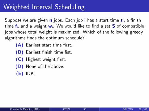
Weighted Interval Scheduling
Suppose we are given n jobs. Each job i has a start time si, a finishtime fi, and a weight wi. We would like to find a set S of compatiblejobs whose total weight is maximized. Which of the following greedyalgorithms finds the optimum schedule?
(A) Earliest start time first.
(B) Earliest finish time fist.
(C) Highest weight first.
(D) None of the above.
(E) IDK.
Weighted problem can be solved via dynamic prog. See notes.
Chandra & Manoj (UIUC) CS374 38 Fall 2015 38 / 40
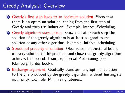
Greedy Analysis: Overview
1 Greedy’s first step leads to an optimum solution. Show thatthere is an optimum solution leading from the first step ofGreedy and then use induction. Example, Interval Scheduling.
2 Greedy algorithm stays ahead. Show that after each step thesolution of the greedy algorithm is at least as good as thesolution of any other algorithm. Example, Interval scheduling.
3 Structural property of solution. Observe some structural boundof every solution to the problem, and show that greedy algorithmachieves this bound. Example, Interval Partitioning (seeKleinberg-Tardos book).
4 Exchange argument. Gradually transform any optimal solutionto the one produced by the greedy algorithm, without hurting itsoptimality. Example, Minimizing lateness.
Chandra & Manoj (UIUC) CS374 39 Fall 2015 39 / 40

Takeaway Points
1 Greedy algorithms come naturally but often are incorrect. Aproof of correctness is an absolute necessity.
2 Exchange arguments are often the key proof ingredient. Focuson why the first step of the algorithm is correct: need to showthat there is an optimum/correct solution with the first step ofthe algorithm.
3 Thinking about correctness is also a good way to figure outwhich of the many greedy strategies is likely to work.
Chandra & Manoj (UIUC) CS374 40 Fall 2015 40 / 40
Related Documents