GraphVar: a brief tutorial for getting started

Outline:

1. Example investigation: „chilli contest“ (global and local efficiency) 2. Group comparison (global efficiency) 3. Raw connectivity matrix and Network Based Statistics 4. Within design I (change of efficiency T1 T2 between sex) 5. Within design II (change of efficiency and behavior T1 T2)

GraphVar: a brief tutorial for getting started

Interpreting GraphVar output

d: Difference between Group Means

F(df1,df2): F-value

d(b): Difference between Standardized Regression Weights

b: Standardized Regression Weight

t(df): t-Value

p: p-Value

m: Mean

significant

not-significant

Hypothesis: 1. Chilli eating champs probably have more efficient brains… otherwise they could not deal with all the pain! 2. Probably orbito frontal gyrus and supplementary motor area contribute here… something like value representations and motor inhibition (… „don´t spit out these delicious chillies“)

1. Example investigation: „chilli contest“ (global and local efficiency)

Hypothesis: … a potential confound could be how much beer somebody had to drink before (i.e., cooling effect on the brain)

1. Use the right mouse to start GraphVar by clicking RUN on the „start_GraphVar“ script in the main folder

2. Create a new Workspace „Chilli_Contest“

• The demo (default) data selection window appears (refer to the manual for how to change this)

• Research_site and sex are initially not selected as these variables are encoded as

strings in the variable spread sheet … you may select them if you want

• Hit the okay button (or simply close the window)

• Selected variables will be loaded in the „statistics window“

• FYI: there is also a help button in the top right! • When help is enabled, you will have a mouse over info most functions of the GUI

• Now, select the subjects (in general settings) • Navigate to the „Sample Workspace“ and select subject 20-30 • Path: …GraphVar/workspaces/SampleWorkspace/data/CorrMatrix

• A selection windows appears asking for the array in the CorrMatrix .mat file in which the correlations are saved (here this is CorrMatrix)

• The name will subsequently appear in the Corr Matrix Array box

• Highlight the subject ID with the mouse to provide the reference between the CorrMatrices and the subject data in the variable spreadsheet (these should be identical)

• If you don´t want to do statistics (only calculation of graph metrics and export) no spreadsheet is required

• Now, you´ll have to specify a network in the network construction panel (by default AAL labels are loaded) -> the network nodes/brain areas refer to the „brain regions file“ (see manual)

• For this tutorial we specify the „chilly-responsive-network“:

starting from Precentral gyrus (left) until Insula (right) -> select the 30 consecutive nodes with your mouse or keyboard

• Here, we want to construct different networks using relative thresholding (i.e., densities) • Simply select all the thresholds in the box with „ctrl+A“ (see manual for how to add more thresholds)

• For this investigation let´s construct subject specific null-model networks to calculate „small-worldness“

• Here, we ONLY generate 10 binary random networks per subject per threshold using the „randomizer_bin_und“ BCT function (for small-worldness, normalization purposes, or non-parametric testing you would normally use 100-1000 or even more … but this will take a lot of time)

• As we have the hypothesis, that chilli eating champs probably have more efficient brains and that probably insula and orbito frontal cortex may contribute here, we select: Binary: Efficiency global Binary: Efficiency local

• Select also “Use random network to calc smallworldness”

• FYI: you can also add custom functions (see appendix in the manual); also note that for some of the functions it would not make sense to do statistics on (e.g., modularity affiliation vector; get components)

• In the GLM panel add „eating_contest_chilli“ and „beer_pong_score“ as predictors in the between covariates field

• Also select the option to perform permuation testing with 1000 permutations per threshold

Parallel Computing (with toolbox)

• If you have the parallel computing toolbox installed, you may want to use more workers (cores) to speed up the generation of null-model networks!

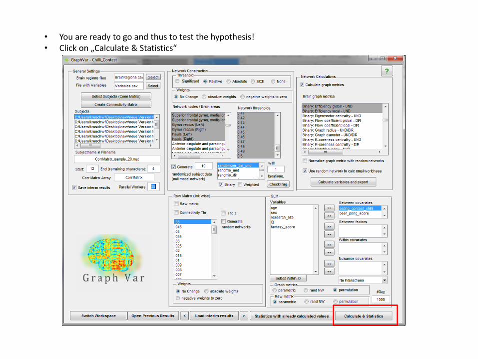
• You are ready to go and thus to test the hypothesis! • Click on „Calculate & Statistics“

• This computation will take about 2-3 minutes …

• This is the results viewer

• To see the results for global efficiency across thresholds, select the „eating_contest_chilli“, „beer_pong_score“, „efficiency_bin“, and all thresholds (ctrl+A)

• Selection of brain areas does not have an effect on global variables • FYI: the „Intercept“ is the constant in the GLM (i.e., expected mean value of Y when all X=0)

• Now, you should see the association of chilli eating contest scores, beer pong scores to global efficiency • The red dots indicate where the correlation is significant according to the desired alpha level

(which you can change here)

• To explore the p-values across thresholds select the „show p-Values“ button • By hitting the button again the correlation appears again

• To plot the non-parametric prediction of chilli scores and global efficiency derived from the random data (null-model distribution with 1000 permutations per threshold), select only „eating_contest_chilli“, select the correction method „Random Networks/Groups“ and click in „show randomize…“

• The confidence intervall (according to the selected alpha) and the null-model distribution appears • You can drag and drop the legend box

The plot of random data is reduced to maximally 100 to make the programm faster

• You can also explore the overlap of the parametric und non-parametric p-values • Here, non-parametric p-values are nearly identical to the parametric distribution

• By scaling down the thresholds, we notice that the association of global efficiency and chilli eating scores starts at a threshold of 0.19

• Driven by this beautiful association of global efficiency and chilli eating scores, we now decide to explore the local efficiencies of all the regions in our chilli-responsive-network across the threshold range 0.19-0.5

• Specify the threshold range and select the Graphvar „efficiency_local_bin“

• Here you see the association of local efficiency of each of the 30 regions in the network to the chilli score • Notice the mouse over box telling you the area, threshold, beta, and p-value

• FYI: it is possible to hide all non-significant associations

• If we a-priori determined that only significant associations on minimally 10 thresholds would be meaningful, we can use the build in filter function and set the number on 9 (i.e., thr > 9)

• Subsequently, the viewer will only show the areas with the specified criteria • Note that these regions are highlighted in the „Brain Areas“ field. • All subsequent actions will only apply to these regions (e.g. filtering) • If you want the full network again you will have to select all nodes (ctrl+A) • If you have an a-prioir hypothesis on specific structures you can also simply select those in

the „Brain Areas“ field

• You can also change the properties of the colour map (right mouse click on the colour map)

• Also use the colour map editor to set the range of correlations in the clolour bar (e.g., -1 to 1)

• We think that these results are meaningful and decide to save and to export these to a csv file (which we open with excel later on)

• Only things that are visible in the results window will be exported Everything we have computed (global efficiency and local efficiency across thresholds) may be saved

Hypothesis – confirmed! 1. YES - Chilli eating champs probably have more efficient brains… otherwise they could not deal with all the pain! 2. YES - orbito frontal gyrus and the olfactory gyrus contribute here…with a positive correlation of local efficiency to chilli eating … much more spicy information transfer here!

Interpretation

2. Group comparison (global efficiency)

• Now, we can also go back and decide to to a group comparison (ANOVA) on the previously calculated efficiencies, where we regress out the influence of IQ and compute the model on the residuals

• Add „research site“ as a „between factor“, add „IQ“ as „nuisance covariate“ and „test against 1000 perm“ • Finally hit „Statistics with already calculated values“

• You see the distribution of F values across thresholds for the group differences (i.e., factor research site) on global efficiency and small-worldness

• Red dots again indicate significance

• Plot the paramteric and non-parametric p-values …

• Select only „efficiency_bin“ • Exlplore how the groups contribute to this effect by selecting „Show/Hide group value“

• Examine the mean of „efficiency_bin“ for each single group (i.e., significance test against zero) • The blue line shows the group mean for the selected group

• Perform pair-wise comparisons by switching through the group contrasts (here: London vs. NewYork) • The blue line shows the group difference for the specific contrast

• Examine the permutation testing derived null-model distribution for the selected contrast • You can see how the confidence intervall will change with decreasing alpha values (e.g. 0.001)

3. Raw Conn Matrix and Network Based Statistics

• Let´s try some computations on the raw correlation matrices! • Deselect „Calculate graph metrics“ and only use the following setting in:

• This is the interaction of age and IQ and the raw connectivities between the nodes in the 30x30 matrix

• Show only the significant brain areas for the selected interaction by selecting the „hide non significant“ button

• FYI: in the „brain areas field“ you can also select only some areas to be plottet

• Select the non-parametric results and apply the Bonferroni corretion method: observe also the corresponding corrected alpha level (you may also try FDR correction)

• You can now perform NBS! Note that for NBS the selected correction method will provide the p-values for the „initial-link-thresholding“ (here we take the non-parametric Bonferroni corrected p-values)

• Hit the „NBS“ button (for the „get component button please refer to the PDF „new features beta 0.62“)

• The initial-link threshold is carried over from the results viewer (here: non-parametric) • And observe a significant graph component comprised of 12 nodes for the interaction • The selection box allows you to plot positive and/or negative associations (here we only have positive) • Please refer to the Manual for how to interpret and to use the Network Inspector

• Also use the „show all labels“ and „Enable Mouse Over“ to explore this component

• You can export the graph component in matrix format (.csv) but also in Pajeck (PAJ) format for other visualization purposes

• You can also directly open the graph component in BrainNetViewer (Xia et al.) if this nice viewer is installed • INFO: BrainNetViewer mus be added to the MATLAB path with subfolders

4. Within design I (change of

efficiency T1 T2) Research option 1 - example: investigate the association between a constant independent variable (e.g. sex or genotype) and a changing dependent network variable (e.g. efficiency in T1 and T2)

• Select the „Variables_Within_Design“ sheet under …/workspaces/SampleWorkspace • Notice: Scan_ID (one subject = T1: sample_01a, T2: sample_01b) and Subj_ID (sample 1)

Within Variables

Yellow: constant variables repeated Purple: changing variables T1 T2

• Select the „Variables_Within_Design“ sheet under …/workspaces/SampleWorkspace • Notice: Scan_ID (one subject = T1: sample_01a, T2: sample_01b) and Subj_ID (sample 1)

• Select the „Scan_ID“ as file identifier • Select also „Subj_ID“ as subject ID

• Select: age, sex, and IQ

• Navigate to GraphVar/workspaces/SampleWorkspace/data/CorrMatrix_Within_Design • Select all 15 subjects (i.e., 30 files as 1 subject = T1: sample_01a, T2: sample_01b)

• Highlight the Scan_ID • Select all nodes, threshold 0.1, and local efficiency • GLM: sex as between factor

• Click on „Select Within ID“ • And highlight the „Subj_ID“

• The Within deviding field will appear as such on the button • „Calculate & Statistics“

• After Bonferroni correction we can observe a significant difference in change of local efficiency between T1 and T1 as a function of sex (i.e., females as comnpared to males have a stronger change in local efficiency between T1 and T2)

4. Within design II (change of efficiency and behavior T1 T2)

Research option 2 - example: investigate the association between a changing independent variable (e.g. cognitive function in T1 and T2) and the change of a dependent network variable (e.g. network efficiency in T1 T2)

• Select the „Variables_Within_Design“ sheet under …/workspaces/SampleWorkspace • Notice: Scan_ID (one subject = T1: sample_01a, T2: sample_01b) and Subj_ID (sample 1)

Within Variables

Yellow: constant variables repeated Purple: changing variables T1 T2

• Navigate to GraphVar/workspaces/SampleWorkspace/data/CorrMatrix_Within_Design • Select all 15 subjects (i.e., 30 files as 1 subject = T1: sample_01a, T2: sample_01b)

• Highlight the Scan_ID • Select all nodes, all thresholds, binary „Transitivity“

• 1. GLM: select beer_pong_score as within covariate • 2. Select „Subj_ID“ as within dividing field in the automatic pop-up window

• Run 1000 permutations • Calculate & Statistics

• You will obvserve a significant positive association between change in behavior and a change in transitivity in the low threshold range