Graphs and the Jacobian conjecture

Journal of Pure and Applied Algebra 212 (2008) 578–598www.elsevier.com/locate/jpaa

Graphs and the Jacobian conjecture

Arno van den Essen, Roel Willems∗

Radboud University of Nijmegen, Department of Mathematics, Postbus 9100, 6500 GL, Nijmegen, Netherlands

Received 2 March 2007; received in revised form 13 June 2007; accepted 26 June 2007Available online 4 September 2007

Communicated by C.A. Weibel

Abstract

It is proved in [M. de Bondt, A. van den Essen, A reduction of the Jacobian conjecture to the symmetric case, Proceedings ofthe AMS 133 (8) (2005) 2201–2205] that it suffices to study the Jacobian Conjecture for maps of the form x + ∇ f , where f is ahomogeneous polynomial of degree d (=4). The Jacobian Condition implies that f is a finite sum of d-th powers of linear forms,〈α, x〉

d , where 〈x, y〉 = x t y and each α is an isotropic vector i.e. 〈α, α〉 = 0. To a set {α1, . . . , αs} of isotropic vectors, we assigna graph and study its structure in case the corresponding polynomial f =

∑〈α j , x〉

d has a nilpotent Hessian. The main result ofthis article asserts that in the case dim([α1, . . . , αs ]) ≤ 2 or ≥ s − 2, the Jacobian Conjecture holds for the maps x + ∇ f . In fact,we give a complete description of the graphs of such f ’s, whose Hessian is nilpotent. As an application of the result, we show thatlines and cycles cannot appear as graphs of HN polynomials.c© 2007 Elsevier B.V. All rights reserved.

MSC: Primary: 14R15; secondary: 05C99; 31B05

1. Introduction

Let F := ( f1, . . . , fn) : Cn→ Cn be a polynomial mapping. And let J F := (

∂ fi∂x j

)n×n denote the Jacobian Matrix

of F . The condition “det J F ∈ C∗” is called the Jacobian Condition.The Jacobian Condition is a necessary condition for a polynomial mapping to be invertible. Whether it is also a

sufficient condition is still an open problem.Jacobian Conjecture (JC).If F : Cn

→ Cn satisfies the Jacobian Condition, then F is invertible.This conjecture, which originates from a paper by Ott-Heinrich Keller in 1939, is the main subject of this article.

Since it was originally formulated by Keller, it is also known as “Keller’s Problem”. In 1998, Keller’s Problemappeared as Problem 16 on a list of 18 famous open problems in the paper “Mathematical problems for the nextcentury” by Smale [9].

∗ Corresponding author.E-mail addresses: [email protected] (A. van den Essen), [email protected] (R. Willems).

0022-4049/$ - see front matter c© 2007 Elsevier B.V. All rights reserved.doi:10.1016/j.jpaa.2007.06.016

A. van den Essen, R. Willems / Journal of Pure and Applied Algebra 212 (2008) 578–598 579

In the past decades, a number of reductions and alternative formulations of the JC have been proved. Here we onlystate the ones that are important for this article. More details on these reductions and reformulations can be foundin [3].

In [1] Bass, Connell, and Wright and [12] Yagzhev proved that it suffices to study the JC for all n ≥ 1 and allpolynomial maps of the form F = x + H , where H = (H1, . . . , Hn) is homogeneous (of degree 3) and J H isnilpotent.

Next, de Bondt and van den Essen in [2] showed that it suffices to study polynomial mappings of the formF = x + H with J H not only nilpotent but also symmetric. Now let J H be a Jacobian matrix. From Lemma1.3.53 in [6], one easily deduces that J H is symmetric iff H is a gradient mapping, i.e. H = ∇ f (=(

∂ f∂x1

, . . . ,∂ f∂xn

))

for some f ∈ C[x]. Define the Hessian of a polynomial f as H( f ) := J∇ f = (∂2 f

∂xi ∂x j)n×n . They showed that the

following statements are equivalent:

(i) The Jacobian Conjecture.(ii) The Jacobian Conjecture for polynomial maps of the form x + ∇ f with H( f ) nilpotent and f homogeneous of

degree 4.

Using this result, Zhao obtained a remarkable result [13]. Recall that the Laplace operator, denoted by ∆, is equalto ∂2

1 + · · · + ∂2n .

Theorem 1.1. Let f ∈ C[x1, . . . , xn], then

(i) H( f ) is nilpotent ⇔ ∆m( f m) = 0 ∀m ≥ 1.(ii) F := x + ∇ f is invertible ⇔ ∆m( f m+1) = 0 ∀m � 0.

So we are going to investigate polynomial maps of the form F = x + ∇ f ∈ C[x]n with H( f ) nilpotent, using

Theorem 1.1. Such f ∈ C[x] we call Hessian Nilpotent (HN).In Section 2, we remark that for homogeneous polynomials f of degree d, if ∆( f ) = 0, then f can be written

in the form∑

j 〈α j , x〉d , where α j are isotropic vectors. Now let A := {α1, . . . , αs} be a set of non-zero isotropic

vectors. Then we assign a graph G(A) to such a set, where each vertex corresponds to a vector αi , and two verticescorresponding to αi and α j respectively are connected iff 〈αi , α j 〉 6= 0.

We show that it suffices to study sets with connected graphs. And in Section 2.3, we describe a large class of HNpolynomials. In Section 3, we prove the main theorem of this paper. It gives a complete description of all possiblegraphs, of which the corresponding polynomials are Hessian Nilpotent, in case either dim[A] := dim([α1, . . . αs]) ≤ 2or dim[A] ≥ s − 2 and the set A is reduced, which means that no two αi ’s are linearly dependent. More precisely, weshow

Theorem 1.2. Let A = {α1, . . . , αs} be a reduced set of isotropic vectors in Cn and let fA(x) =∑s

j=1〈α j , x〉d with

d ≥ 4. If fA(x) is HN, then

(i) if dim[A] = 1, 2, s, s − 1, then G(A) is totally disconnected, which means that 〈αi , α j 〉 = 0 for all 1 ≤ i, j ≤ s.Furthermore F := x + ∇ fA(x) is invertible.

(ii) if dim[A] = s − 2 and G(A) is connected, then G(A) = K (4, s − 4) and d = 4. Furthermore F := x +∇ fA(x)

is invertible.

Here, K (4, s − 4) means a bipartite graph with four vertices on one side, which are all mutually disconnected andon the other side s − 4 vertices which are also mutually disconnected, and all vertices from one side are connected toall vertices on the other side.

The fact that in both cases of Theorem 1.2 the polynomial mapping F is invertible follows from the followingTheorem, which is proved in Section 3.2.

Theorem 1.3. Let f be of the form g(〈α1, x〉, . . . , 〈αt , x〉), where all αi are linearly independent (over C) vectors inCn and g ∈ C[y1, . . . , yt ]. Let

A := (〈αi , α j 〉)1≤i, j≤t

and r := rank(A). Suppose r ≤ 4. If f is HN, then x + ∇ f is invertible.

580 A. van den Essen, R. Willems / Journal of Pure and Applied Algebra 212 (2008) 578–598

In Section 4, we deduce from Theorem 1.2, that HN polynomials of which the corresponding graph is a line or a cycledo not exist. Furthermore, we give an example of a set of isotropic vectors with the dimension of the span being s − 2and the corresponding polynomial Hessian Nilpotent. Finally in Section 5, we describe sets of isotropic vectors, withcorresponding graphs of the form K (r, t) for all r ≥ 1, t ≥ 4, and we describe a set of isotropic vectors of which thecorresponding graph is not of the form K (r, t) for any r, t .

2. Preliminaries

2.1. Harmonic polynomials

From the reduction in [2] and Theorem 1.1, it follows that in order to investigate the JC, we need to studyhomogeneous Hessian Nilpotent polynomials. We saw that a homogeneous polynomial f is HN, iff ∆m( f m) = 0 forall m ≥ 1. Recall that a function s with ∆(s) = 0 is called harmonic. So a HN polynomial f is harmonic. Now weshow why homogeneous harmonic polynomials are of a special form.

First, we need some notations and generalities. Let O(n) = On(C) be the orthogonal group, i.e. the set of n × nmatrices T with elements in C, such that T tT = In . Furthermore, let Hm be the (finite dimensional) C-vectorspace of homogeneous harmonic polynomials of degree m in n variables. Now Hm is a C[O(n)]-module, whereC[O(n)] is the group ring of O(n), with the following operation: let T ∈ O(n) and P(x) ∈ Hm , and then defineT · P = P(T −1x) = P(T tx).

Theorem 2.1. If Hm 6= 0, then Hm is an irreducible C[O(n)]-module.

A proof of this theorem and the following corollary can be found in [8] (Theorem 5.2.4 and Proposition 5.2.6).Recall that a vector is called isotropic if it is orthogonal to itself, with respect to the standard bilinear form on

Cn , denoted as 〈·, ·〉. So for α = (α1, . . . , αn) ∈ Cn to be isotropic means that 〈α, α〉 =∑n

i=1 α2i = 0. Now from

Theorem 2.1, it follows that

Corollary 2.2. f ∈ Hm if and only if

f =

s∑j=1

〈α j , x〉m (1)

for some s and α j ∈ Cn isotropic vectors.

So in order to investigate HN polynomials, we need to investigate the polynomials of the form (1). From now on,we denote the set of all isotropic vectors in Cn by X (Cn).

2.2. Graphs

Assume that f is a harmonic, homogeneous polynomial of degree d ≥ 2. Then by Corollary 2.2, f can be writtenas:

f (x) =

s∑j=1

hdα j

(x), (2)

for some s ∈ N, where hα j (x) = 〈α j , x〉 and α j ∈ X (Cn).Now we want to investigate when such a polynomial f is HN. Since every (homogeneous) harmonic polynomial

is given by a set of isotropic vectors, we need to study these sets. Note that, given a harmonic polynomial, thecorresponding set of isotropic vectors need not be unique and in fact rarely is. So instead of starting with a harmonicpolynomial, we start with a set of isotropic vectors and then study the corresponding polynomial.

In [13], Zhao introduces two matrices using these isotropic vectors. Let A = {α1, . . . αs} be a set of isotropicvectors, and let fA be the corresponding harmonic polynomial of the form (2). Then define

MA := (〈αi , α j 〉)s×s, (3)

ΨA := (〈αi , α j 〉hd−2α j

(x))s×s . (4)

A. van den Essen, R. Willems / Journal of Pure and Applied Algebra 212 (2008) 578–598 581

In his article, Zhao proves the following proposition:

Proposition 2.3. Let A be a set of isotropic vectors and let fA(x) be the corresponding harmonic (homogeneous)polynomial given by (2). Then for any m ≥ 1, we have

TraceH( fA)m= (d(d − 1))m Trace Ψm

A. (5)

In particular, fA(x) is HN if and only if the matrix ΨA is nilpotent.

So to investigate whether a harmonic function fA(x) is HN, one needs to study the matrix ΨA. With respect to thenilpotency of ΨA, recall the following lemma:

Lemma 2.4. Let M ∈ Ms(C[x]); then M is nilpotent iff the sum of the (r × r) principal minors is zero for all1 ≤ r ≤ rank(M).

This is Wright’s Theorem 2.3 in [11].To make the sets of isotropic vectors more understandable and to make it easier to talk about them, we are going

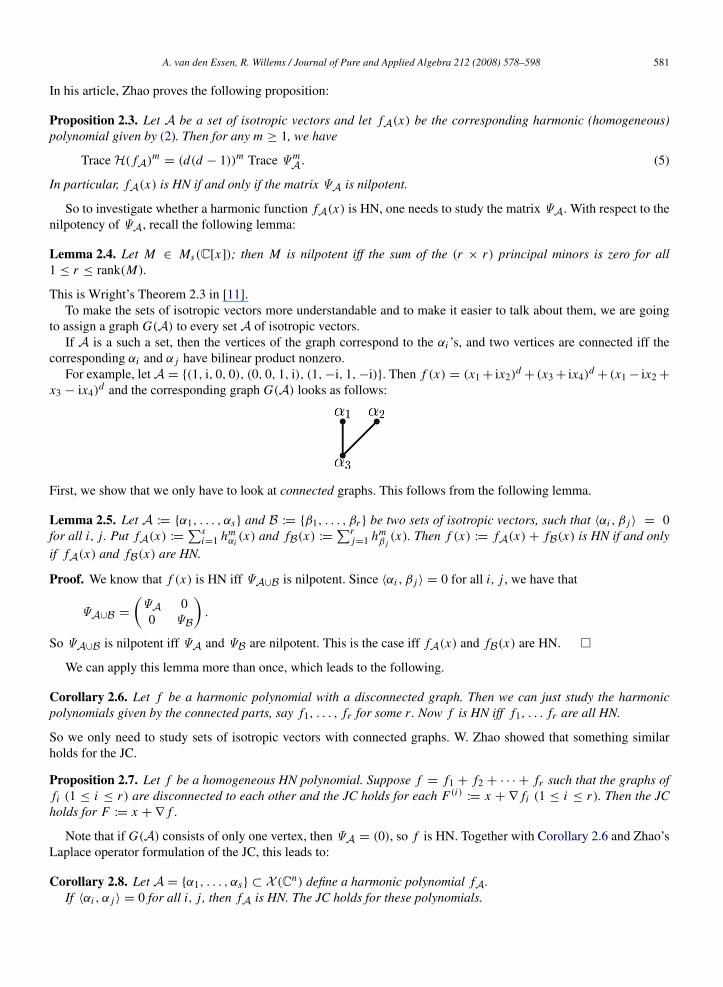
to assign a graph G(A) to every set A of isotropic vectors.If A is a such a set, then the vertices of the graph correspond to the αi ’s, and two vertices are connected iff the

corresponding αi and α j have bilinear product nonzero.For example, letA = {(1, i, 0, 0), (0, 0, 1, i), (1, −i, 1, −i)}. Then f (x) = (x1 + ix2)

d+ (x3 + ix4)

d+ (x1 − ix2 +

x3 − ix4)d and the corresponding graph G(A) looks as follows:

First, we show that we only have to look at connected graphs. This follows from the following lemma.

Lemma 2.5. Let A := {α1, . . . , αs} and B := {β1, . . . , βr } be two sets of isotropic vectors, such that 〈αi , β j 〉 = 0for all i, j . Put fA(x) :=

∑si=1 hm

αi(x) and fB(x) :=

∑rj=1 hm

β j(x). Then f (x) := fA(x) + fB(x) is HN if and only

if fA(x) and fB(x) are HN.

Proof. We know that f (x) is HN iff ΨA∪B is nilpotent. Since 〈αi , β j 〉 = 0 for all i, j , we have that

ΨA∪B =

(ΨA 00 ΨB

).

So ΨA∪B is nilpotent iff ΨA and ΨB are nilpotent. This is the case iff fA(x) and fB(x) are HN. �

We can apply this lemma more than once, which leads to the following.

Corollary 2.6. Let f be a harmonic polynomial with a disconnected graph. Then we can just study the harmonicpolynomials given by the connected parts, say f1, . . . , fr for some r. Now f is HN iff f1, . . . fr are all HN.

So we only need to study sets of isotropic vectors with connected graphs. W. Zhao showed that something similarholds for the JC.

Proposition 2.7. Let f be a homogeneous HN polynomial. Suppose f = f1 + f2 + · · · + fr such that the graphs offi (1 ≤ i ≤ r) are disconnected to each other and the JC holds for each F (i)

:= x + ∇ fi (1 ≤ i ≤ r). Then the JCholds for F := x + ∇ f .

Note that if G(A) consists of only one vertex, then ΨA = (0), so f is HN. Together with Corollary 2.6 and Zhao’sLaplace operator formulation of the JC, this leads to:

Corollary 2.8. Let A = {α1, . . . , αs} ⊂ X (Cn) define a harmonic polynomial fA.If 〈αi , α j 〉 = 0 for all i, j , then fA is HN. The JC holds for these polynomials.

582 A. van den Essen, R. Willems / Journal of Pure and Applied Algebra 212 (2008) 578–598

We will call such a set of isotropic vectors α1, . . . , αs orthogonal or completely disconnected.Now the question arises as to which graphs can appear: for instance, do there exist HN polynomials such that the

graph of that polynomial is a cycle? Another general group of graphs that is of interest, are the so-called bipartitegraphs:

Definition 2.9.

K (r, s) := {α1, . . . , αr } ∪ {β1, . . . , βs},

where αi , β j ∈ X (Cn) for all i, j , such that 〈αi , α j 〉 = 0, 〈βi , β j 〉 = 0 and 〈αi , β j 〉 6= 0.

A special subclass of K (r, s), is formed by the so-called shrubs S(r) := K (r, 1).

2.3. The class Hess(n, R)

In this section, we will describe a class Hess(n, R) of polynomials over a commutative ring R, that contains asquare root of −1, and we prove that all polynomials in this class are HN.

Definition 2.10. Let R be a commutative ring with an element i, such that i2 = −1. Now let

• Hess(0, R) := R,• Hess(1, R) := Rx1 + R.

For n ≥ 2, f ∈ Hess(n, R) ⊆ R[x1, . . . , xn] iff there exist c0, . . . , cn ∈ R, T ∈ O(n, R) and g ∈ Hess(n−2, R[t])such that

f (T x) = g(x1, . . . , xn−2)|t=xn−1+ixn +

n∑j=1

c j x j + c0. (6)

So the first nontrivial class becomes

Example 2.11. Hess(2, R).f ∈ Hess(2, R) ⊆ R[x1, x2] iff there exist c0, c1, c2 ∈ R, T ∈ O(2, R) and g ∈ R[t] such that

f (T x) = g(x1 + ix2) + c1x1 + c2x2 + c0.

First, we prove

Lemma 2.12. Let f (x) ∈ R[x1, . . . , xn] and T ∈ O(n, R). Then f (T x) is HN iff f (x) is HN.

Proof. Since we know that f (x) is HN iffH( f (x)) is nilpotent, we know that the following statements are equivalent

• f (T x) is HN iff f (x) is HN.• H( f (T x)) is nilpotent iffH( f (x)) is nilpotent.

But the second statement follows from the fact that H( f (T x)) = T tH( f (x))|T x T and the fact that T t= T −1

(since T ∈ O(n, R)). �

Lemma 2.13. Let g(x1, . . . , xn−2, xn−1 + ixn) ∈ R[x1, . . . , xn].Hx1,...,xn−2(g) is nilpotent iff H(g) is nilpotent.

Proof. To simplify notation, we write H forHx1,...,xn−2(g). One can verify (by simply writing it out) that

H(g) =

H u iuut a iaiut ia −a

with u ∈ R[x1, . . . , xn−2]

n−2 and a ∈ R[x1, . . . , xn−2]. By induction on r , one can prove that

H(g)r=

H r H r−1u iH r−1u(H r−1u)t b ibi(H r−1u)t ib −b

for some b ∈ R[x1, . . . , xn−2]. It follows that ifH(g)r

= (0), then H r= (0).

A. van den Essen, R. Willems / Journal of Pure and Applied Algebra 212 (2008) 578–598 583

The other way around: if H r= (0), then

H(g)r=

0 v ivvt b ibivt ib −b

with v = H r−1u and b ∈ R[x1, . . . , xn−2]. Then vtv = (H r−1u)t H r−1u = ut(H r−1)2u = 0, because H is symmetricand r ≥ 2. But thenH(g)2r

= (0). �

Now we can prove the following theorem.

Theorem 2.14. Let f ∈ R[x1, . . . , xn]. If f ∈ Hess(n, R), thenH( f ) is nilpotent.

Proof. It is clear that if f ∈ Hess(0, R) or f ∈ Hess(1, R), then H( f ) is nilpotent. So with Lemma 2.12 andDefinition 2.10, we have that

f (x) is HN ⇔ f (T x) is HN (7)

⇔ g(x1, . . . xn−2, xn−1 + ixn) +

n∑j=1

c j x j + c0 is HN (8)

⇔ g(x1, . . . xn−2, xn−1 + ixn) is HN (9)

⇔ Hx1,...,xn−2(g) is nilpotent. (10)

Statement (10) follows from Lemma 2.13. So the theorem follows by induction on n. �

A large class of HN polynomials, which we will use in Section 4.3 below, is described in the following corollary.

Corollary 2.15. Let f ∈ C[x1, . . . , xn], with n even, be of the form g(x1 + ix2, . . . , xn−1 + ixn) + (x3 − ix4 + · · · +

xn−1 − ixn)h(x1 + ix2) for some g ∈ C[y1, . . . , yn/2] and h ∈ C[y]. Then f is HN.

Proof. From Definition 2.10 and by induction on n, it follows that f ∈ Hess(n, C), so the conclusion follows fromTheorem 2.14. �

3. Proof of the main theorem

Throughout the remainder of this article, letA = {α1, . . . , αs} be a set of isotropic vectors. We write l = dim[A] :=

dim([α1, . . . , αs]), where [α1, . . . , αs] denotes the C-span of α1, . . . , αs . We may also assume that α1, . . . , αl arelinearly independent and that αl+1, . . . , αs ∈ [α1, . . . , αl ]; this can easily be accomplished by a rearrangment ofα1, . . . , αs . Furthermore let

Tl :=

αt1...

αtl

∈ Ml×n(C),

be the l × n-matrix, with αti on the i-th row. Tl has rank l, so we can extend Tl to an invertible n × n-matrix TA. Now

if we substitute T −1A x for x , then for i ≤ l we have that

hαi (T −1A x)d

:= 〈αi , T −1A x〉

d= 〈αt

i T−1A , x〉

d= 〈ei , x〉

d= xd

i , (11)

where ei denotes the i-th standard basis vector.Doing the same substitution, for i > l, so αi =

∑lj=1 λ jα j for some λ j ∈ C, we get:

hαi (T −1A x)d

=

(l∑

j=1

λ j x j

)d

. (12)

If, given a set of isotropic vectors α1, . . . , αs , we can show that 〈αi , α j 〉 = 0, then with Corollary 2.8, the polynomialthey represent is HN and for that polynomial the JC holds. So a way to prove that the JC holds for some class of

584 A. van den Essen, R. Willems / Journal of Pure and Applied Algebra 212 (2008) 578–598

polynomials is to show that their sets of isotropic vectors are orthogonal. We start with a few lemmas, which areelementary, so we leave the proofs to the reader – they can also be found in [10].

Lemma 3.1 (Linear Dependency of Two Isotropic Vectors). Let α1, α2 ∈ X (Cn). If α1, α2 are linearly dependent,say α2 = λα1 with λ 6= 0 ∈ C, then

hdα1

(x) + hdα2

(x) = hdα(x).

with α =d√

1 + λdα1. �

In this manner, we can reduce a set of isotropic vectors until there does not exist a pair of linearly dependent isotropicvectors. Such a set we will call reduced. For the remainder of this article, we assume that a given set of isotropicvectors is reduced.

Lemma 3.2 (Three Dependent Isotropic Vectors). Let α1, α2, α3 ∈ X (Cn), such that α3 = λ1α1 + λ2α2, withλ1, λ2 6= 0. Then 〈αi , α j 〉 = 0 for all i, j .

From now on, we assume that d ≥ 4.Note that for most of the proofs given in the remainder of this subsection, we only use the fact that the sum of the

(2 × 2) principal minors of ΨA has to be zero in order for fA(x) to be HN, which is clearly a weaker condition thanfA(x) is HN.

The following lemma, whose proof follows easily from (11), describes the set of isotropic vectors, if dim[A] = s.

Lemma 3.3 (Independent Isotropic Vectors). Let A := {α1, . . . , αs} ⊂ X (Cn), that defines a harmonic polynomialfA(x). If α1, . . . , αs are linearly independent and fA(x) is HN, then 〈αi , α j 〉 = 0 for all 1 ≤ i, j ≤ s.

The next lemma gives a similar result when dim[A] is minimal.

Lemma 3.4 (Dimension of [α1, . . . , αs] ≤ 2). LetA := {α1, . . . , αs} ⊂ X (Cn), which defines a harmonic polynomialfA(x), where dim[A] ≤ 2 and A is reduced. If fA(x) is HN, then 〈αi , α j 〉 = 0 for all i, j .

The following lemma deals with the case where dim[A] = s − 1. Since the technique used in this proof is similarto the ones used in the proof of Theorem 1.2(ii), we give the proof as an appetizer.

Lemma 3.5 (Dimension of [α1, . . . , αs] = s − 1). Let A := {α1, . . . , αs} ⊂ X (Cn) define a harmonic polynomialfA(x), with dim[A] = s − 1 and A reduced. If fA(x) is HN, then 〈αi , α j 〉 = 0 for all i, j .

Proof. We may assume that α1, . . . , αs−1 are linearly independent and that αs ∈ [α1, . . . , αs−1]. Since {α1, . . . , αs}

is reduced, we may assume that αs =∑s−1

i=1 λiαi and that there are at least two i’s for which λi 6= 0. Using the factthat the sum of the (2 × 2) principal minors of ΨA has to be zero for fA(x) to be HN, we get that∑

1≤i< j≤s

〈αi , α j 〉2he

αi(x)he

α j(x) = 0,

where e = d − 2. Substituting T −1A x for x , we get

0 =

∑1≤i< j≤s−1

〈αi , α j 〉2xe

i xej +

s−1∑i=1

〈αi , αs〉2xe

i

(s−1∑j=1

λ j x j

)e

. (13)

Remember that the xi are independent. Now fix 1 ≤ i ≤ s − 1. Then there are two possibilities:

(1) If λi 6= 0, then on the right hand side of the equality there appears one term of the form x2ei with coefficient

〈αi , αs〉2λe

i , which has to be zero because the xi are independent. Because λi 6= 0, we have that 〈αi , αs〉 = 0.(2) If λi = 0, then there exist 1 ≤ l < m ≤ s − 1 for which λl , λm are nonzero. Then there exists a term of the form

xei xl xe−1

m with coefficient e〈αi , αs〉2λlλ

e−1m , which has to be zero because the xi are independent. Since λl , λm are

nonzero, we have that 〈αi , αs〉 = 0.

We now have that 〈αi , αs〉 = 0 for 1 ≤ i ≤ s − 1. Using Lemmas 2.5 and 3.3, we get that 〈αi , α j 〉 = 0 for alli, j . �

A. van den Essen, R. Willems / Journal of Pure and Applied Algebra 212 (2008) 578–598 585

3.1. Proof of Theorem 1.2

Theorem 1.2(i) follows from Lemmas 3.3–3.5, and Corollary 2.8. Next we prove part (ii).

Proof of Theorem 1.2(ii). For the remainder of this subsection, we assume that A = {α1, . . . , αs} ⊂ X (Cn), withA reduced, dim[A] = s − 2, G(A) connected and fA is HN. Furthermore, we may assume that, after a suitablepermutation of α1, . . . , αs , the vertices α1, . . . , αs−2 are linearly independent and αs−1, αs ∈ [α1, . . . , αs−2]. Thenwe can write:

αs−1 =

s−2∑j=1

λ jα j (14)

αs =

s−2∑j=1

µ jα j (15)

with λ j , µ j ∈ C. Define

Es−1 = {i |λi 6= 0} (16)

Es = {i |µi 6= 0}. (17)

Note that since A is reduced, we have #Es−1 ≥ 2 and #Es ≥ 2.Also note that since fA is HN, it follows from Proposition 2.3, that ΨA is nilpotent. According to Lemma 2.4 this

is equivalent to the fact that the sum of the (m × m) principal minors of ΨA is zero for 1 ≤ m ≤ s. In particular, thesum of the (2 × 2) principal minors of ΨA is zero, which means that∑

1≤i< j≤s

〈αi , α j 〉2he

αi(x)he

α j(x) = 0

where e = d − 2 ≥ 2. Now substituting T −1A x for x ,it follows from (11) and (12) that

f2(x) :=

∑1≤i< j≤s−2

〈αi , α j 〉2xe

i xej +

(s−2∑i=1

〈αi , αs−1〉2xe

i

)L(x)e

+

(s−2∑i=1

〈αi , αs〉2xe

i

)M(x)e

+ 〈αs−1, αs〉2L(x)e M(x)e

= 0, (18)

where

M(x) =

s−2∑j=1

µ j x j

L(x) =

s−2∑j=1

λ j x j .

The proof is in six steps:

(1) First we show that d = 4.(2) Second we prove that Es−1 = Es .(3) Then we show that 〈αs−1, αs〉 = 0.(4) Next we prove that

αs−1 = λ1αs−3 + λ2αs−2,

αs = µ1αs−3 + µ2αs−2,

with λ1, λ2, µ1, µ2 ∈ C∗.(5) Then we show that G(A) = K (4, s − 4).(6) Finally, we prove that F := x + ∇ fA is invertible.

586 A. van den Essen, R. Willems / Journal of Pure and Applied Algebra 212 (2008) 578–598

The fact that d = 4 follows from the following lemma, a proof of which can be found in [5].

Lemma 3.6. Let k ≥ 3 and R(y1, . . . , yr+2) ∈ C[y1, . . . , yr+2], where degyi(R(y)) ≤ 1 ∀i and λ, µ ∈ Cr such that

R(zk1, . . . , zk

r , (λ1z1 + · · · + λr zr )k, (µ1z1 + · · · + µr zr )

k) = 0.

Then either λ = λi ei or µ = µi ei with ei is the i th unit vector in Cr for some i or λ and µ are linearly dependent.

Since α1, . . . , αs−2 are linearly independent, we also have that 〈α1, x〉, . . . , 〈αs−2, x〉 are linearly independent.Furthermore, we have that 〈αs−1, x〉

k= (λ1〈α1, x〉 + · · · + λs−2〈αs−2, x〉)k and that 〈αs, x〉

k= (µ1〈α1, x〉 + · · · +

µs−2〈αs−2, x〉)k . If we define zi := 〈αi , x〉 for 1 ≤ i ≤ s − 2, then f2(x) gives us exactly such a relation as describedin Lemma 3.6, with k = e = d − 2. So if k ≥ 3, which means that d ≥ 5, then either αs−1 = λiαi for some i orαs = λiαi for some i , which would mean that A is not reduced. Or αs−1 and αs are linearly dependent, but againthat would mean that A is not reduced. Since we assumed that A was reduced, we know that d ≤ 4. Because we alsoassumed d ≥ 4, we have that d = 4.

The second claim follows from the following lemma:

Lemma 3.7. Let A be as above, then Es−1 = Es .

Proof. We will show that (i) if Es−1 6⊆ Es , then αs−1 is an isolated vertex. Similarly, one can show that(ii) if Es 6⊆ Es−1, then αs is an isolated vertex. Since we assumed that G(A) was connected, we get that Es−1 = Es .

It remains to prove (i) and (ii).Proof of (i): Suppose that i0 ∈ Es−1, but i0 6∈ Es . Now we rewrite

f2(x) = A(x)L(x)e+ B(x),

where

A(x) =

s−2∑i=1

〈αi , αs−1〉2xe

i + 〈αs−1, αs〉2 M(x)e

B(x) =

∑1≤i< j≤s−2

〈αi , α j 〉2xe

i xej +

s−2∑i=1

〈αi , αs〉2xe

i M(x)e.

In L(x)e, there is a nonzero monomial whose xi0 -degree is 1; however, any nonzero monomial appearing in A(x) orB(x) has xi0 -degree equal to 0 or e ≥ 2. So A(x)L(x)e

+ B(x) = 0 implies that A(x) = 0. Suppose j0, j1 ∈ Es . Then,since x j0 xe−1

j1appears as a monomial in M(x)e, we get that 〈αs−1, αs〉 = 0, because the xi are independent variables.

And this together with A(x) = 0 implies that 〈αi , αs〉 = 0, again because the xi ’s are independent variables. Whichmeans that αs is an isolated vertex.

The proof of (ii) goes similarly. �

The third claim follows from the following lemma.

Lemma 3.8. Let A as above; then 〈αs−1, αs〉 = 0.

Proof. If #Es−1 = 2, then 〈αs−1, αs〉 = 0 (with Lemma 3.2). So assume that #Es−1 ≥ 3. Then for all subsets{ j1, j2, j3} ⊂ Es−1. we look at the coefficients of x2e

j1, x2e−1

j1x j2 , x2e−1

j1x j3 of f2(x) and get:

λej1 µe

j1 λej1µ

ej1

λe−1j1

λ j2 µe−1j1

µ j2 λe−1j1

λ j2µej1 + λe

j1µe−1j1

µ j2

λe−1j1

λ j3 µe−1j1

µ j3 λe−1j1

λ j3µej1 + λe

j1µe−1j1

µ j3

〈α j1 , αs−1〉

2

〈α j1 , αs〉2

〈αs−1, αs〉2

=

000

(19)

and

det

λe

j1 µej1 λe

j1µej1

λe−1j1

λ j2 µe−1j1

µ j2 λe−1j1

λ j2µej1 + λe

j1µe−1j1

µ j2

λe−1j1

λ j3 µe−1j1

µ j3 λe−1j1

λ j3µej1 + λe

j1µe−1j1

µ j3

= −λ2e−1j1

µ2e−1j1

det(

λ j2 µ j2λ j3 µ j3

).

A. van den Essen, R. Willems / Journal of Pure and Applied Algebra 212 (2008) 578–598 587

If

det(

λ j2 µ j2λ j3 µ j3

)= 0

for all j2, j3, then αs−1 = καs for a κ ∈ C. This is impossible, because we assumed that {α1, . . . , αs} was reduced.So there is at least one pair j2, j3 such that

det(

λ j2 µ j2λ j3 µ j3

)6= 0,

But then, the 3 × 3 matrix in (19) is invertible, whence 〈αs−1, αs〉 = 0. �

The fourth claim follows from the next lemma:

Lemma 3.9. Let A again be as above. Then we can rearrange α1, . . . , αs−2 such that

αs−1 = λs−3αs−3 + λs−2αs−2, (20)

αs = µs−3αs−3 + µs−2αs−2, (21)

with λs−3, λs−2, µs−3, µs−2 ∈ C∗.

Proof. Note that this is equivalent to showing that #Es−1 = 2.If for every pair j2, j3 ∈ Es−1 we have

det(

λ j2 µ j2λ j3 µ j3

)= 0,

then αs−1 = καs , which is impossible because {α1, . . . , αs} is reduced. So there is at least one pair j2, j3 ∈ Es−1such that

det(

λ j2 µ j2λ j3 µ j3

)6= 0.

Now assume that #Es−1 ≥ 3, i.e. ∃ j1 ∈ Es−1, j1 6∈ { j2, j3}. For m = 1, . . . , s − 2 look at the coefficients ofxe

m xe−1j1

x j2 and of xem xe−1

j1x j3 in f2(x):

xem xe−1

j1x j2 : 〈αm, αs−1〉

2λe−1j1

λ j2 + 〈αm, αs〉2µe−1

j1µ j2 = 0

xem xe−1

j1x j3 : 〈αm, αs−1〉

2λe−1j1

λ j3 + 〈αm, αs〉2µe−1

j1µ j3 = 0.

So (λe−1

j1λ j2 µe−1

j1µ j2

λe−1j1

λ j3 µe−1j1

µ j3

)(〈αm, αs−1〉

2

〈αm, αs〉2

)=

(00

).

But

det

(λe−1

j1λ j2 µe−1

j1µ j2

λe−1j1

λ j3 µe−1j1

µ j3

)= λe−1

j1µe−1

j1det

(λ j2 µ j2λ j3 µ j3

)6= 0.

So by Lemma 3.8 〈αm, αs−1〉 = 〈αm, αs〉 = 0 for all m ∈ {1, . . . , s}. Again, this is in contradiction with theassumption that G(A) is connected. So #Es−1 = 2 as desired. �

The fifth claim follows from:

Lemma 3.10. Let A as above; then G(A) = K (4, s − 4).

Proof. From Eqs. (20) and (21), Lemmas 3.2 and 3.8 it follows that

〈αi , α j 〉 = 0 for i, j ∈ {s − 3, s − 2, s − 1, s}. (22)

588 A. van den Essen, R. Willems / Journal of Pure and Applied Algebra 212 (2008) 578–598

Substituting all previous results in Eq. (18), we get

f2(x) =

∑1≤i< j≤s−4

〈αi , α j 〉2x2

i x2j +

∑1≤i≤s−4

(〈αs−3, αi 〉2x2

s−3x2i + 〈αs−2, αi 〉

2x2s−2x2

i

+ 〈αs−1, αi 〉2(λs−3xs−3 + λs−2xs−2)

2x2i + 〈αs, αi 〉

2(µs−3xs−3 + µs−2xs−2)2x2

i ). (23)

Since f2 = 0 and the xi are algebraically independent variables, it follows that the coefficient of x2i x2

j is zero for1 ≤ i < j ≤ s − 4, from which it immediately follows that

〈αi , α j 〉 = 0 for i, j ∈ {1, . . . , s − 4}. (24)

If 〈αi , α j 〉 = 0 for some i ∈ {1, . . . , s − 4} and all j ∈ {s − 3, s − 2, s − 1, s}, then G(A) is not connected. So wehave that for every i ∈ {1, . . . , s − 4}, there is a j ∈ {s − 3, s − 2, s − 1, s} such that 〈αi , α j 〉 6= 0. We show belowthat for all i ∈ {1, . . . , s − 4}, the following holds:

〈αi , α j 〉 6= 0 for a j ∈ {s − 3, s − 2, s − 1, s} ⇒ 〈αi , α j 〉 6= 0 for all j ∈ {s − 3, s − 2, s − 1, s}. (25)

Now let β1 := αs−3, β2 := αs−2, β3 := αs−1, β4 := αs . Consider the set {α1, . . . , αs−4, β1, . . . , β4}. It thenfollows from the Eqs. (22) and (24) and statement (25) that 〈αi , β j 〉 6= 0 and 〈αi , α j 〉 = 〈βi , β j 〉 = 0 for all i, j . SoG(A) = K (4, s − 4).

It remains to prove statement (25). Observe that if there exists a j ∈ {s − 3, s − 2, s − 1, s} such that 〈αi , α j 〉 6= 0,then either 〈αi , αs−3〉 6= 0, or 〈αi , αs−2〉 6= 0, because of the Eqs. (20) and (21). So 〈αi , α j 〉 6= 0 for j = s − 3 orj = s − 2. Then look at the coefficient of xe

i xej in f2:

〈αi , α j 〉2+ 〈αi , αs−1〉

2λ2j + 〈αi , αs〉

2µ2j = 0. (26)

Since 〈αi , α j 〉 6= 0, it follows from Eq. (26) that either 〈αi , αs−1〉 6= 0 or 〈αi , αs〉 6= 0. Furthermore, looking at thecoefficient of x2

i xs−3xs−2 gives:

〈αi , αs−1〉2λs−3λs−2 + 〈αi , αs〉

2µs−3µs−2 = 0.

So if both 〈αi , αs−1〉 and 〈αi , αs〉 are nonzero, then they are both nonzero. So since G(A) is connected, itfollows that for all i ∈ {1, . . . , s − 4}, we have that 〈αi , αs−1〉 6= 0 and 〈αi , αs〉 6= 0. Now define A′

:=

{α1, . . . , αs−4, αs−1, αs, αs−3, αs−2}. Then A′ satisfies exactly the same conditions as A, and applying the aboveargument to A′ shows that for all i ∈ {1, . . . , s − 4}, we have that 〈αi , αs−3〉 6= 0, 〈αi , αs−2〉 6= 0. This provesstatement (25). �

To prove the sixth and last claim, we use Theorem 1.3. First we show that fA can be written in the form as describedin Theorem 1.3.

Let A = {α1, . . . , αs} ⊂ X (Cn). Let fA be the corresponding harmonic polynomial, and let t := dim[A]. Thenwe can rearrange the α’s in such a manner that α1, . . . , αt are linearly independent and αt+1, . . . , αs ∈ [α1, . . . , αt ].So

αi =

t∑j=1

λi, jα j , (27)

for t + 1 ≤ i ≤ s.We deduce that

fA =

s∑i=1

〈αi , x〉d

=

t∑i=1

〈αi , x〉d

+

s∑i=t+1

⟨t∑

j=1

λi, jα j , x

⟩d

(28)

=

t∑i=1

〈αi , x〉d

+

s∑i=t+1

(t∑

j=1

λi, j 〈α j , x〉

)d

. (29)

So f = g(〈α1, x〉, . . . , 〈αt , x〉) for some g ∈ C[y1, . . . , yt ]. So every polynomial fA can be written in the form ofTheorem 1.3. Let A be as in Theorem 1.3. Then rank(A) ≤ rank(MA). So to prove the last claim of Theorem 1.2, weneed to show that rank(MA) ≤ 4. This will be done in the following lemma.

A. van den Essen, R. Willems / Journal of Pure and Applied Algebra 212 (2008) 578–598 589

Lemma 3.11. Let A be as above. Then rank(MA) ≤ 4.

Proof. Then from Lemma 3.10, it follows that

MA =

∅

〈α1, αs−3〉 〈α1, αs−2〉 〈α1, αs−1〉 〈α1, αs〉...

......

...

〈αs−4, αs−3〉 〈αs−4, αs−2〉 〈αs−4, αs−1〉 〈αs−4, αs〉

〈α1, αs−3〉 . . . 〈αs−4, αs−3〉

〈α1, αs−2〉 . . . 〈αs−4, αs−2〉

〈α1, αs−1〉 . . . 〈αs−4, αs−1〉

〈α1, αs〉 . . . 〈αs−4, αs〉

∅

.

From Lemma 3.9, it follows that the last two rows are linearly dependent of the s − 3-th and the s − 2-nd row.Similarly, the last two columns are linearly dependent of the s − 3-th and the s − 2-nd columns. So the dimension ofthe row-space generated by the last four rows is less than or equal to two. The dimension of the row-space generatedby the first s − 4 rows is equal to the dimension of the column-space generated by the last four columns, which is alsoless than or equal to two. This means that rank(MA) ≤ 4. �

This proves Theorem 1.2. �

3.2. Proof of Theorem 1.3

LetA = {α1, . . . , αs} be a set of isotropic vectors, such that the corresponding polynomial fA =∑

i hdαi

(x) is HNand such that rank(MA) ≤ 4. Then F := x + ∇ fA is invertible. This result is due to Michiel de Bondt, Arno van denEssen and Sherwood Washburn, but remained unpublished. See also [7]. To prove it, we need the following theorem.Let R be an arbitrary Q-algebra.

Theorem 3.12. Let f ∈ R[x1, . . . , xn] with n ≤ 4, and let F := x + ∇ f . If J (∇ f ) is nilpotent, then F is invertible.

Proof. (i) First, we assume that R is a domain. Since J (∇ f ) is nilpotent, it follows that det(J F) = 1. Let R − 0 bethe finitely generated Q-subalgebra of R generated by the coefficients of f . So R0 is Noetherian. By [6], Lemma1.1.13 we can view R0 as a subring of C and F as a polynomial map over C. Then by [4], Theorem 5.1 F isinvertible over C. Since F ∈ R0[x]

n and det(J F) = 1, it follows from [6], Lemma 1.1.8 that F is invertible overR0 and hence over R.

(ii) Now let R be an arbitrary (Q)-algebra. Replacing R by R0, we may assume that R is Noetherian. Furthermoreby [6], Lemma 1.1.9 we may assume that R is reduced. In particular, (0) = p1 ∩ · · · ∩ pr for some finite set ofprime ideals pi of R.

(iii) Since for each i R/pi is a domain, it follows from (i) that F is invertible over R/pi (where F is obtainedby reducing its coefficients mod pi ). Then a wellnknown argument (see for example part (iii) in the proof ofPropisition 1.1.12 in [6] gives that F is invertible over R. �

To formulate the next lemma, we introduce some notations.Let f be of the form g(〈α1, x〉, . . . , 〈αt , x〉), where α1, . . . , αt ∈ Cn are linearly independent over C and

g ∈ C[y1, . . . , yt ]. Put

A := (〈αi , α j 〉)1≤i, j≤t

and let r := rank(A).Then it is well known that there exists a T ∈ Glt (C) such that

T t AT =

(Ir 00 0

).

Furthermore, define: (α1 · · · αt ) := (α1 · · · αt )T , z := T t y andg(z) := g((T t)−1z) (=g(y)). With those notations, we get

Lemma 3.13. (i) f = g(〈α1, x〉, . . . , 〈αt , x〉).

590 A. van den Essen, R. Willems / Journal of Pure and Applied Algebra 212 (2008) 578–598

(ii) T t AT = (〈αi , α j 〉)1≤i, j≤t .(iii) If we put H := ∇ f , then J H is nilpotent iff Hz1,...,zr (g), the Hessian of g with respect to z1, . . . , zr , where g is

viewed as a polynomial in z1, . . . , zr with coefficients in C[zr+1, . . . , zt ], is nilpotent.

Proof. (i) follows directly from the definitions above. (ii) follows readily from Lemma 1.3 from [7]: just replaceeverywhere n − 1 by t . Finally, (iii) follows from the proof of Corollary 1.4 in the same article. �

Now we can give.

Proof of Theorem 1.3. As above choose T ∈ Glt (C), such that

T t AT =

(Ir 00 0

).

If we replace αi by αi and g by g, we are in the situation that f = g(〈α1, x〉, . . . , 〈αt , x〉), where α1, . . . , αt ∈ Cn arelinearly independent over C, g ∈ C[y1, . . . , yt ] and

A =

(Ir 00 0

).

Furthermore, if we put H := ∇ f , then from Lemma 3.13(iii) and the hypothesis that f is HN, it follows that

Hy1,...,yr (g(y1, . . . , yt )) is nilpotent. (30)

We want to deduce that F is invertible if r ≤ 4.Since α1, . . . , αt are linearly independent, we can extend the matrixαt

1...

αtt

∈ Mt×n(C)

to an invertible n × n matrix

M :=

αt1...

αtt

β tt+1...

β tn

,

for suitable βt+1, . . . , βn ∈ Cn .Then we have that

Mx =

〈α1, x〉

...

〈αt , x〉

〈βt+1, x〉

...

〈βn, x〉

.

If we now consider g as a polynomial in C[y1, . . . , yn], then g(Mx) = g(〈α1, x〉, . . . , 〈αt , x〉) = f . So we have that

J f = (Jg)(Mx)M = (gy1(Mx), . . . , gyt (Mx), 0, . . . , 0)

αt1...

αtt

β tt+1...

β tn

.

A. van den Essen, R. Willems / Journal of Pure and Applied Algebra 212 (2008) 578–598 591

And thus

∇ f =(α1 · · · αt βt+1 · · · βn

)

gy1(Mx)...

gyt (Mx)

0...

0

.

Now consider

F = x + ∇ f = x + M t

gy1(Mx)...

gyt (Mx)

0...

0

.

Then F is invertible iff F ◦ (M−1x) is invertible iff M F ◦ (M−1x) is invertible. This leads to F is invertible iff

x + M M t

gy1(x)...

gyt (x)

0...

0

is invertible.

Now

M M t=

αt1...

αtt

β tt+1...

β tn

(α1 · · · αt βt+1 · · · βn

)=

(A CC t D

),

for some C ∈ Mt×n−t (C) and D ∈ Mn−t×n−t (C). And this leads to

M M t

gy1(x)...

gyt (x)

0...

0

=

(Ir ∅

∅ ∅t−r

)C

C t D

gy1(x)...

gyt (x)

0...

0

=

gy1(x)...

gyr (x)

0...

0

C t

gy1(x)...

gyt (x)

.

592 A. van den Essen, R. Willems / Journal of Pure and Applied Algebra 212 (2008) 578–598

So F is invertible iff

x1 + gx1(x1, . . . xt )...

xr + gxr (x1, . . . xt )

xr+1...

xtxt+1 + Pt+1(x1, . . . , xt )

...

xn + Pn(x1, . . . , xt )

is invertible. After composing with the elementary transformations

xt+1 7−→ xt+1 − Pt+1(x1, . . . , xt )

...

xn 7−→ xn − Pn(x1, . . . , xt )

we get that F is invertible iff

x1 + gx1(x1, . . . xt )...

xr + gxr (x1, . . . xt )

xr+1...

xn

is invertible. If we now consider g as a polynomial in C[xr+1, . . . , xn][x1, . . . , xr ], i.e. as a polynomial in r variablesover the ring C[xr+1, . . . , xn], then the result follows from (30) and Theorem 3.12. �

We have shown that for a set A of isotropic vectors with rank(MA) ≤ 4, such that the corresponding polynomialfA(x) is HN, the Jacobian Conjecture is true.

4. Applications of Theorem 1.2

Let A := {α1, . . . , αs} ⊂ X (Cn), and fA be the corresponding harmonic polynomial of degree d ≥ 4. DefineMA := (〈αi , α j 〉)1≤i, j≤s .

Note that if s < 5, it follows from Theorem 1.2 that G(A) is totally disconnected, because dim[A] ∈ {1, 2, s−1, s}.Since we are only interested in sets A with G(A) connected, we may always assume that s ≥ 5.

First, we show that if fA is HN, then G(A) is not a line. Secondly, we prove that if fA is HN, then G(A) isnot a cycle. Finally we give, for every s ≥ 5, an example of an HN polynomial fA(x) with G(A) connected anddim[A] = s − 2.

4.1. HN polynomials where G(A) is a line do not exist

Suppose we have a set A = {α1, . . . , αs} ⊂ X (Cn), which defines a harmonic polynomial fA(x) and with G(A)

a line. Then we have that

A. van den Essen, R. Willems / Journal of Pure and Applied Algebra 212 (2008) 578–598 593

MA =

0 a1 0 . . . 0a1 0 a2 0 . . . 00 a2 0 a3 0 . . . 0...

. . .. . .

. . .. . .

. . ....

0 . . . 0 as−3 0 as−2 00 . . . 0 as−2 0 as−10 . . . 0 as−1 0

where ai = 〈αi , αi+1〉 6= 0.

Lemma 4.1. Let A = {α1, . . . , αs}, with s ≥ 5, and MA as above. Then rank(MA) ≥ s − 1.

Proof. If we remove from MA the first column and the last row, we get a lower triangular matrix with determinant∏s−1i=1 ai 6= 0. So this matrix has maximal rank, which is s − 1. It follows that rank(MA) ≥ s − 1. �

Now we can prove the following:

Theorem 4.2. The non-existence of A with G(A) a line.LetA := {α1, . . . , αs} ⊂ X (Cn) be such thatA is reduced and G(A) is connected, which defines a HN polynomial

fA. If G(A) is a line, then s = 1.

Proof. Suppose G(A) is a line. With Lemma 4.1, we have that rank(MA) ≥ s − 1, but rank(MA) ≤ dim[A]. Sodim[A] ≥ s − 1, but from Theorem 1.2(i), then it follows that G(A) is totally disconnected. So the only possible setA with G(A) a line is A = {α}. �

4.2. HN polynomials with cyclic graphs do not exist

Suppose we have a set A := {α1, . . . , αs} that defines an HN polynomial fA, where G(A) is cyclic. Then MAwould be symmetric and look as follows

MA =

0 a1 0 . . . 0 asa1 0 a2 0 . . . 00 a2 0 a3 0 . . . 0...

. . .. . .

. . .. . .

. . ....

0 . . . 0 as−3 0 as−2 00 . . . 0 as−2 0 as−1as 0 . . . 0 as−1 0

,

with ai = 〈αi , αi+1〉, as = 〈αs, α1〉and ai 6= 0 ∀i .

Lemma 4.3. Let A = {α1, . . . , αs}, with s ≥ 5, and MA as above. Then rank(MA) ≥ s − 2.

Proof. If we remove the first two columns and the first and the last rows of mA, we get a lower triangular matrix withdeterminant

∏s−1i=2 ai 6= 0, so the rank of this matrix is maximal, which is s −2. It follows that rank(MA) ≥ s −2. �

Now we can prove the following:

Theorem 4.4. The non-existence of a cyclic G(A).Let A := {α1, . . . , αs} ⊂ X (Cn) such that A is reduced and G(A) is connected, which defines a HN polynomial

fA. Then G(A) is not a cycle.

Proof. Suppose G(A) is a cycle. With Lemma 4.3, we have that rank(MA) ≥ s − 2. But rank(MA) ≤ dim[A]. Sodim[A] ≥ s −2. But from Theorem 1.2(ii), it follows that either G(A) is totally disconnected or G(A) = K (4, s −4).In both cases, G(A) is not a cycle. �

594 A. van den Essen, R. Willems / Journal of Pure and Applied Algebra 212 (2008) 578–598

4.3. The existence of a HN polynomial fA with dim[A] = s − 2

In this subsection, we describe a class of sets A ⊂ X (Cn) with dim[A] = s − 2 and G(A) connected for all s ≥ 5such that fA is HN.

We denote by e j the j-th standard basis vector in Cn .

Example 4.5. Let n = 2s − 6, and define

α j := e2 j+1 + ie2 j+2 for 1 ≤ j ≤ s − 4,

αs−3 :=

s−4∑j=1

(e2 j+1 − ie2 j+2) + e1 + ie2,

αs−2 :=

s−4∑j=1

(−e2 j+1 + ie2 j+2) + e1 + ie2,

αs−1 :=

s−4∑j=1

(ie2 j+1 + e2 j+2) + e1 + ie2,

αs :=

s−4∑j=1

(−ie2 j+1 − e2 j+2) + e1 + ie2.

Then let A := {α1, . . . , αs} and define

fA(x) :=

s−3∑j=1

〈α j , x〉4− 〈αs−2, x〉

4− i〈αs−1, x〉

4+ i〈αs, x〉

4. (31)

It is easily seen that α1, . . . , αs−2 are linearly independent, and one can also verify that

αs−1 =12(1 + i)αs−3 +

12(1 − i)αs−2,

αs =12(1 − i)αs−3 +

12(1 + i)αs−2.

Now define g(y) ∈ C[y1, y2, y3, y4] as follows:

g(y) := 〈(1, i, 1, −i), (y1, y2, y3, y4)〉4− 〈(1, i, −1, i), (y1, y2, y3, y4)〉

4

− i〈(1, i, i, 1), (y1, y2, y3, y4)〉4+ i〈(1, i, −i, −1), (y1, y2, y3, y4)〉

4

= 16(y1 + iy2)3(y3 − iy4).

Then we have that

fA(x) =

s−4∑j=1

(x2 j+1 + ix2 j+2)4+ g

(x1, x2,

s−4∑j=1

x2 j+1,

s−4∑j=1

x2 j+2

)

=

s−4∑j=1

(x2 j+1 + ix2 j+2)4+ 16(x1 + ix2)

3

(s−4∑j=1

x2 j+1 − is−4∑j=1

x2 j+2

)

=

s−4∑j=1

(x2 j+1 + ix2 j+2)4+ 16(x1 + ix2)

3

(s−4∑j=1

(x2 j+1 − ix2 j+2)

).

So fA is of the form as described in Corollary 2.15, and hence fA is HN. Furthermore, we have that

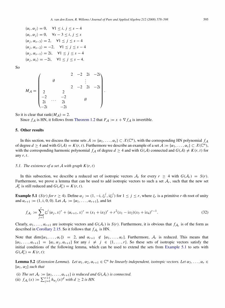
A. van den Essen, R. Willems / Journal of Pure and Applied Algebra 212 (2008) 578–598 595

〈αi , α j 〉 = 0, ∀1 ≤ i, j ≤ s − 4

〈αi , α j 〉 = 0, ∀s − 3 ≤ i, j ≤ s

〈α j , αs−3〉 = 2, ∀1 ≤ j ≤ s − 4

〈α j , αs−2〉 = −2, ∀1 ≤ j ≤ s − 4

〈α j , αs−1〉 = 2i, ∀1 ≤ j ≤ s − 4

〈α j , αs〉 = −2i, ∀1 ≤ j ≤ s − 4.

So

MA =

∅

2 −2 2i −2i...

2 −2 2i −2i2

−22i

−2i

. . .

2−22i

−2i

∅

.

So it is clear that rank(MA) = 2.Since fA is HN, it follows from Theorem 1.2 that FA := x + ∇ fA is invertible.

5. Other results

In this section, we discuss the some sets A := {α1, . . . , αs} ⊂ X (Cn), with the corresponding HN polynomial fAof degree d ≥ 4 and with G(A) = K (r, t). Furthermore we describe an example of a setA := {α1, . . . , αs} ⊂ X (Cn),with the corresponding harmonic polynomial fA of degree d ≥ 4 and with G(A) connected and G(A) 6= K (r, t) forany r, t .

5.1. The existence of a set A with graph K (r, t)

In this subsection, we describe a reduced set of isotropic vectors Ar for every r ≥ 4 with G(Ar ) = S(r).Furthermore, we prove a lemma that can be used to add isotropic vectors to such a set Ar , such that the new setAt

r is still reduced and G(Atr ) = K (r, t).

Example 5.1 (S(r) for r ≥ 4). Define α j := (1, −i, ζ jr , iζ j

r ) for 1 ≤ j ≤ r , where ζr is a primitive r -th root of unityand αr+1 := (1, i, 0, 0). Let Ar := {α1, . . . , αr+1}, and let

fAr :=

r∑j=1

ζj

r 〈α j , x〉r+ 〈αr+1, x〉

r= (x1 + ix2)

r+ r2(x1 − ix2)(x3 + ix4)

r−1. (32)

Clearly, α1, . . . , αr+1 are isotropic vectors and G(Ar ) is S(r). Furthermore, it is obvious that fAr is of the form asdescribed in Corollary 2.15. So it follows that fAr is HN.

Note that dim([α1, . . . , αr ]) = 2, and αr+1 6∈ [α1, . . . , αr ]. Furthermore, Ar is reduced. This means that[α1, . . . , αr+1] = [αi , α j , αr+1] for any i 6= j ∈ {1, . . . , r}. So these sets of isotropic vectors satisfy theinitial conditions of the following lemma, which can be used to extend the sets from Example 5.1 to sets withG(At

r ) = K (r, t):

Lemma 5.2 (Extension Lemma). Let α1, α2, αr+1 ∈ Cn be linearly independent, isotropic vectors. Let α3, . . . , αr ∈

[α1, α2] such that

(i) The set Ar := {α1, . . . , αr+1} is reduced and G(Ar ) is connected.(ii) fAr (x) :=

∑r+1j=1 hα j (x)d with d ≥ 2 is HN.

596 A. van den Essen, R. Willems / Journal of Pure and Applied Algebra 212 (2008) 578–598

Further let µ, ν ∈ C be such that µ 6= 0, ν 6= 0, and µ〈α1, αr+1〉+ν〈α2, αr+1〉 = 0. Now choose αr+2, . . . , αr+t ∈

[µα1 + να2, αr+1], in such a manner that the coefficient of αr+1 is nonzero and the set Atr := {α1, . . . , αr+t } is

reduced. Then we have that

fAtr(x) :=

r+t∑j=1

hα j (x)d

is HN. Furthermore, FAtr

:= x + ∇ fAtr

is invertible.

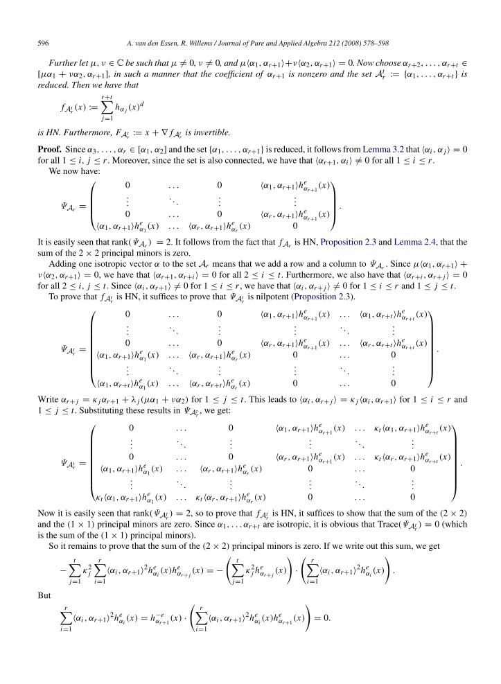
Proof. Since α3, . . . , αr ∈ [α1, α2] and the set {α1, . . . , αr+1} is reduced, it follows from Lemma 3.2 that 〈αi , α j 〉 = 0for all 1 ≤ i, j ≤ r . Moreover, since the set is also connected, we have that 〈αr+1, αi 〉 6= 0 for all 1 ≤ i ≤ r .

We now have:

ΨAr =

0 . . . 0 〈α1, αr+1〉h

eαr+1

(x)

.... . .

......

0 . . . 0 〈αr , αr+1〉heαr+1

(x)

〈α1, αr+1〉heα1

(x) . . . 〈αr , αr+1〉heαr

(x) 0

.

It is easily seen that rank(ΨAr ) = 2. It follows from the fact that fAr is HN, Proposition 2.3 and Lemma 2.4, that thesum of the 2 × 2 principal minors is zero.

Adding one isotropic vector α to the set Ar means that we add a row and a column to ΨAr . Since µ〈α1, αr+1〉 +

ν〈α2, αr+1〉 = 0, we have that 〈αr+1, αr+i 〉 = 0 for all 2 ≤ i ≤ t . Furthermore, we also have that 〈αr+i , αr+ j 〉 = 0for all 2 ≤ i, j ≤ t . Since 〈αi , αr+1〉 6= 0 for 1 ≤ i ≤ r , we have that 〈αi , αr+ j 〉 6= 0 for 1 ≤ i ≤ r and 1 ≤ j ≤ t .

To prove that fAtr

is HN, it suffices to prove that ΨAtr

is nilpotent (Proposition 2.3).

ΨAtr

=

0 . . . 0 〈α1, αr+1〉heαr+1

(x) . . . 〈α1, αr+t 〉heαr+t

(x)

.... . .

......

. . ....

0 . . . 0 〈αr , αr+1〉heαr+1

(x) . . . 〈αr , αr+t 〉heαr+t

(x)

〈α1, αr+1〉heα1

(x) . . . 〈αr , αr+1〉heαr

(x) 0 . . . 0...

. . ....

.... . .

...

〈α1, αr+t 〉heα1

(x) . . . 〈αr , αr+t 〉heαr

(x) 0 . . . 0

.

Write αr+ j = κ jαr+1 + λ j (µα1 + να2) for 1 ≤ j ≤ t . This leads to 〈αi , αr+ j 〉 = κ j 〈αi , αr+1〉 for 1 ≤ i ≤ r and1 ≤ j ≤ t . Substituting these results in ΨAt

r, we get:

ΨAtr

=

0 . . . 0 〈α1, αr+1〉heαr+1

(x) . . . κt 〈α1, αr+1〉heαr+t

(x)

.... . .

......

. . ....

0 . . . 0 〈αr , αr+1〉heαr+1

(x) . . . κt 〈αr , αr+1〉heαr+t

(x)

〈α1, αr+1〉heα1

(x) . . . 〈αr , αr+1〉heαr

(x) 0 . . . 0...

. . ....

.... . .

...

κt 〈α1, αr+1〉heα1

(x) . . . κt 〈αr , αr+1〉heαr

(x) 0 . . . 0

.

Now it is easily seen that rank(ΨAtr) = 2, so to prove that fAt

ris HN, it suffices to show that the sum of the (2 × 2)

and the (1 × 1) principal minors are zero. Since α1, . . . αr+t are isotropic, it is obvious that Trace(ΨAtr) = 0 (which

is the sum of the (1 × 1) principal minors).So it remains to prove that the sum of the (2 × 2) principal minors is zero. If we write out this sum, we get

−

t∑j=1

κ2j

r∑i=1

〈αi , αr+1〉2he

αi(x)he

αr+ j(x) = −

(t∑

j=1

κ2j he

αr+ j(x)

)·

(r∑

i=1

〈αi , αr+1〉2he

αi(x)

).

Butr∑

i=1

〈αi , αr+1〉2he

αi(x) = h−e

αr+1(x) ·

(r∑

i=1

〈αi , αr+1〉2he

αi(x)he

αr+1(x)

)= 0.

A. van den Essen, R. Willems / Journal of Pure and Applied Algebra 212 (2008) 578–598 597

This last equality holds because it is the sum of the (2 × 2) principal minors of fAr , which is HN. This proves thatΨAt

ris nilpotent, so fAt

ris HN.

Since we assumed that dim[Atr ] = 3, we have that rank(MAt

r) ≤ 3. It follows from Theorem 1.3 that

FAtr

:= x + ∇ fAtr

is invertible, and therefore the JC holds for these polynomials. �

5.2. An example of a set A with G(A) 6= K (r, t)

In this subsection, we describe a set of isotropic vectors A with fA HN and G(A) connected, but G(A) 6= K (r, t)for any r, t ∈ N.

Let

α1 := (1, i, 0, 0, 0, 0),

α2 := (1, −i, 1, i, 0, 0),

α3 := (−1, i, 1, i, 0, 0),

α4 := (i, 1, 1, i, 0, 0),

α5 := (−i, −1, 1, i, 0, 0),

α6 := (0, 0, 1, i, 0, 0),

α7 := (0, 0, 1, −i, 1, i),

α8 := (0, 0, −1, i, 1, i),

α9 := (0, 0, i, 1, 1, i),

α10 := (0, 0, −i, −1, 1, i).

Then we have that α1, α2, α3, α7, α8 are linearly independent. Furthermore, we have that

α4 =12(1 + i)α2 +

12(1 − i)α3,

α5 =12(1 − i)α2 +

12(1 + i)α3,

α6 =12α2 +

12α3,

α9 =12(1 + i)α7 +

12(1 − i)α8,

α10 =12(1 − i)α7 +

12(1 + i)α8.

Now let A := {α1, . . . , α10}, and define

P(x) := 〈α1, x〉4+ 〈α2, x〉

4− 〈α3, x〉

4− i〈α4, x〉

4+ i〈α5, x〉

4,

Q(x) := 〈α6, x〉4+ 〈α7, x〉

4− 〈α8, x〉

4− i〈α9, x〉

4+ i〈α10, x〉

4,

and

Rλ,µ(x) := λ · P(x) + µ · Q(x)

for λ, µ ∈ C∗.

Then P(x), Q(x), Rλ,µ(x) are HN. Since rank(MA) = 4, we have from Theorem 1.3 that F := x + ∇ Rλ,µ(x) isinvertible. (One can easily see G(A) 6= K (r, t) for any r, t ∈ N.)

Note that G({α1, . . . , α5}) = G({α6, . . . , α10}) = S(4).

598 A. van den Essen, R. Willems / Journal of Pure and Applied Algebra 212 (2008) 578–598

Acknowledgements

The authors would like to thank the referee for various helpful suggestions, especially for the proof of Lemma 3.7and the final step in Lemma 3.11, which improved the proof of Theorem 1.2(ii) considerably. The second author wassupported by the Netherlands Organisation for Scientific Research (NWO).

References

[1] H. Bass, E. Connell, D. Wright, The Jacobian conjecture: Reduction of degree and formal expansion of the inverse, Bulletin of the AmericanMathematical Society 7 (1982) 287–330.

[2] M. de Bondt, A. van den Essen, A reduction of the Jacobian conjecture to the symmetric case, Proceedings of the AMS 133 (8) (2005)2201–2205.

[3] M. de Bondt, A. van den Essen, Recent progress on the Jacobian conjecture, Annales Polonici Mathematici 87 (2005) 1–11.[4] M. de Bondt, A. van den Essen, Nilpotent symmetric Jacobian matrices and the Jacobian conjecture II, Journal of Pure and Applied Algebra

196 (2005) 135–148.[5] M. de Bondt, H. Tong, Power linear Keller maps with ditto triangularizations, Report No. 0603, Radboud Univ. of Nijmegen, 2006.[6] A. van den Essen, Polynomial Automorphisms and the Jacobian Conjecture, in: Progress in Math., vol. 190, Birkhauser, Basel, 2000.[7] A. van den Essen, S. Washburn, The Jacobian conjecture for symmetric Jacobian matrices, Journal of Pure and Applied Algebra 189 (2004)

123–133.[8] R. Goodman, N. Wallach, Representations and Invariants of the Classical Groups, in: Encyclopedia of Mathematics and its Applications, vol.

68, Cambridge Univ. Press, 1998.[9] S. Smale, Mathematical problems for the next century, The Mathematical Intelligencer 20 (2) (1998) 7–15.

[10] R. Willems, Graphs and the Jacobian conjecture, M.Sc. Thesis, Radboud Univ. of Nijmegen, 2005.[11] D. Wright, Formal inverse expansion and the Jacobian conjecture, Journal of Pure and Applied Algebra 48 (1987) 199–219.[12] A. Yagzhev, On Keller’s problem, Siberian Mathematical Journal 21 (1980) 747–754.[13] W. Zhao, Hessian nilpotent polynomials and the Jacobian conjecture, Transactions of the AMS 359 (1) (2007) 249–274.