Graph Planning for Environmental Coverage · 2011-08-09 · For this work, we model the set of coverage problems as arc routing problems. Al-though these routing problems are generally

Graph Planning for Environmental Coverage

Ling Xu

CMU-RI-TR-11-24

Submitted in partial fulfillment of the

requirements for the degree of

Doctor of Philosophy in Robotics

The Robotics Institute

Carnegie Mellon University

Pittsburgh, Pennsylvania 15213

August 2011

Thesis Committee:

Anthony Stentz (co-chair)

Omead Amidi (co-chair)

Howie Choset

John Krumm, Microsoft Research

Copyright c© 2011 by Ling Xu. All rights reserved.

For my grandparents

iv

Abstract

Tasks such as street mapping and security surveillance seek a route that traverses

a given space to perform a function. These task functions may involve mapping the

space for accurate modeling, sensing the space for unusual activity, or searching the

space for objects. When these tasks are performed autonomously by robots, the con-

straints of the environment must be considered in order to generate more feasible

paths. Additionally, performing these tasks in the real world presents the challenge

of operating in dynamic, changing environments.

This thesis addresses the problem of effective graph coverage with environmental

constraints and incomplete prior map information. Prior information about the en-

vironment is assumed to be given in the form of a graph. We seek a solution that

effectively covers the graph while accounting for space restrictions and online changes.

For real-time applications, we seek a complete but efficient solution that has fast re-

planning capabilities.

For this work, we model the set of coverage problems as arc routing problems. Al-

though these routing problems are generally NP-hard, our approach aims for optimal

solutions through the use of low-complexity algorithms in a branch-and-bound frame-

work when time permits and approximations when time restrictions apply. Addition-

ally, we account for environmental constraints by embedding those constraints into

the graph. In this thesis, we present algorithms that address the multi-dimensional

routing problem and its subproblems and evaluate them on both computer-generated

and physical road network data.

vi

Funding

This work was partially sponsored by the U.S. Army Research Laboratory contract

of the Robotics Collaborative Technology Alliance (contract number DAAD19-01-2-

0012) and the Collaborative Technology Alliance Program, Cooperative Agreement

W911NF-10-2-0016. The views and conclusions contained in this document are those

of the authors and should not be interpreted as representing the official policies or

endorsements of the U.S. Government. Additionally, this work was sponsored by the

ONR Contract Number N00014-09-1-1031.

viii

Acknowledgments

First, I would like to thank my advisors Tony and Omead. Your guidance and

encouragement has been invaluable throughout this PhD process. I would also like

to thank my committee members, John and Howie, for taking the time to meet with

me and giving great feedback on the thesis. Thanks to the rCommerce and helicopter

labs for the facilities and technical support which allowed me to run various tests both

on and offline. A big thanks to Suzanne who deserves the “RI Cool Person” award

every year.

Many people have made my graduate experience wonderful. Thanks to Bernardine,

Joyce, and the Techbridgeworld team for giving me the opportunity to see technology

in a new light. Many thanks to Carol, Mary, and the Women@SCS group for teaching

me the importance of outreach. My friends both at CMU and outside have truly made

Pittsburgh home – thanks for all the fun times!

Thanks to all my family especially my parents for your support and encouragement

and my parents-in-law for your enthusiasm and multiple trips out to Pittsburgh.

Thanks to Carolyn for always being a phone call away. Finally, thanks to Jevan for

your patience and love throughout the past six years.

x

Contents

1 Introduction 1

1.1 Types of Problems . . . . . . . . . . . . . . . . . . . . . . . . . . . . . . . . . . . . 2

1.1.1 Mapping . . . . . . . . . . . . . . . . . . . . . . . . . . . . . . . . . . . . . . 4

1.1.2 Search . . . . . . . . . . . . . . . . . . . . . . . . . . . . . . . . . . . . . . . 4

1.1.3 Patrol . . . . . . . . . . . . . . . . . . . . . . . . . . . . . . . . . . . . . . . 6

2 Problem Statement 7

3 Background and Related Work 9

3.1 Model Construction . . . . . . . . . . . . . . . . . . . . . . . . . . . . . . . . . . . 9

3.1.1 Next Best View . . . . . . . . . . . . . . . . . . . . . . . . . . . . . . . . . . 9

3.1.2 Active Exploration . . . . . . . . . . . . . . . . . . . . . . . . . . . . . . . . 10

3.2 Continuous Coverage Planning . . . . . . . . . . . . . . . . . . . . . . . . . . . . . 11

3.2.1 Robot-size Coverage Device . . . . . . . . . . . . . . . . . . . . . . . . . . . 11

3.2.2 Infinite-size Coverage Device . . . . . . . . . . . . . . . . . . . . . . . . . . 12

3.2.3 Extended-range Coverage Device . . . . . . . . . . . . . . . . . . . . . . . . 13

3.3 Comparison of Existing Work . . . . . . . . . . . . . . . . . . . . . . . . . . . . . . 13

3.4 Graph Theoretical Problems . . . . . . . . . . . . . . . . . . . . . . . . . . . . . . . 14

3.4.1 Vertex Routing Problems . . . . . . . . . . . . . . . . . . . . . . . . . . . . 14

3.4.2 Art Gallery and Watchman Problems . . . . . . . . . . . . . . . . . . . . . 15

3.4.3 Arc Routing Problems . . . . . . . . . . . . . . . . . . . . . . . . . . . . . . 16

3.5 Approach . . . . . . . . . . . . . . . . . . . . . . . . . . . . . . . . . . . . . . . . . 21

4 Partial Coverage with a Single Robot without Environmental Constraints 23

4.1 Approach Algorithms . . . . . . . . . . . . . . . . . . . . . . . . . . . . . . . . . . 24

4.1.1 Chinese Postman Problem . . . . . . . . . . . . . . . . . . . . . . . . . . . . 24

4.1.2 Rural Postman Problem . . . . . . . . . . . . . . . . . . . . . . . . . . . . . 25

4.1.3 Online Changes . . . . . . . . . . . . . . . . . . . . . . . . . . . . . . . . . . 29

4.1.4 Farthest Distance Heuristic . . . . . . . . . . . . . . . . . . . . . . . . . . . 32

4.2 Comparison Tests . . . . . . . . . . . . . . . . . . . . . . . . . . . . . . . . . . . . . 35

xi

4.2.1 Rectilinear Graphs . . . . . . . . . . . . . . . . . . . . . . . . . . . . . . . . 37

4.2.2 Real-world Example . . . . . . . . . . . . . . . . . . . . . . . . . . . . . . . 37

4.2.3 Metrics . . . . . . . . . . . . . . . . . . . . . . . . . . . . . . . . . . . . . . 37

4.3 Results . . . . . . . . . . . . . . . . . . . . . . . . . . . . . . . . . . . . . . . . . . . 38

4.3.1 Rectilinear Graphs . . . . . . . . . . . . . . . . . . . . . . . . . . . . . . . . 38

4.3.2 Real-world Example . . . . . . . . . . . . . . . . . . . . . . . . . . . . . . . 39

4.3.3 Evaluation of the Coverage Algorithm . . . . . . . . . . . . . . . . . . . . . 39

4.3.4 Discussion . . . . . . . . . . . . . . . . . . . . . . . . . . . . . . . . . . . . . 40

4.4 Market-based Parallel Branch-and-bound . . . . . . . . . . . . . . . . . . . . . . . 42

4.4.1 Approach . . . . . . . . . . . . . . . . . . . . . . . . . . . . . . . . . . . . . 44

4.4.2 Testing Framework . . . . . . . . . . . . . . . . . . . . . . . . . . . . . . . . 47

4.4.3 Results . . . . . . . . . . . . . . . . . . . . . . . . . . . . . . . . . . . . . . 48

4.4.4 Discussion . . . . . . . . . . . . . . . . . . . . . . . . . . . . . . . . . . . . . 52

4.5 Conclusion . . . . . . . . . . . . . . . . . . . . . . . . . . . . . . . . . . . . . . . . 52

5 Partial Coverage with Multiple Robots without Environmental Constraints 55

5.1 Cluster First, Route Second Approach . . . . . . . . . . . . . . . . . . . . . . . . . 56

5.1.1 Improved k-RPP Algorithm . . . . . . . . . . . . . . . . . . . . . . . . . . . 57

5.1.2 Dynamic k-RPP Algorithm . . . . . . . . . . . . . . . . . . . . . . . . . . . 61

5.1.3 Comparison Tests . . . . . . . . . . . . . . . . . . . . . . . . . . . . . . . . 63

5.1.4 Results . . . . . . . . . . . . . . . . . . . . . . . . . . . . . . . . . . . . . . 64

5.2 Route First, Cluster Second Approach . . . . . . . . . . . . . . . . . . . . . . . . . 69

5.2.1 k-RPP Approximation: Approximation Algorithm for RPP . . . . . . . . . 69

5.2.2 k-RPP Approximation: Optimal Algorithm for RPP . . . . . . . . . . . . . 71

5.3 Conclusion . . . . . . . . . . . . . . . . . . . . . . . . . . . . . . . . . . . . . . . . 74

6 Partial Coverage with Multiple Robots with Environmental Constraints 75

6.1 Approach . . . . . . . . . . . . . . . . . . . . . . . . . . . . . . . . . . . . . . . . . 76

6.1.1 Mixed Rural Postman Problem . . . . . . . . . . . . . . . . . . . . . . . . . 76

6.1.2 Mixed Chinese Postman Problem . . . . . . . . . . . . . . . . . . . . . . . . 77

6.2 k-Mixed Rural Postman Problem . . . . . . . . . . . . . . . . . . . . . . . . . . . . 79

6.2.1 Route First, Cluster Second Approach . . . . . . . . . . . . . . . . . . . . . 81

6.2.2 Cluster First, Route Second Approach . . . . . . . . . . . . . . . . . . . . . 81

6.2.3 Online Changes with Single and Multiple Robots . . . . . . . . . . . . . . . 82

6.3 Testing Framework . . . . . . . . . . . . . . . . . . . . . . . . . . . . . . . . . . . . 83

6.3.1 Test Graphs . . . . . . . . . . . . . . . . . . . . . . . . . . . . . . . . . . . . 83

6.3.2 Static k-MRPP Tests . . . . . . . . . . . . . . . . . . . . . . . . . . . . . . 83

6.3.3 Dynamic Tests . . . . . . . . . . . . . . . . . . . . . . . . . . . . . . . . . . 83

6.3.4 Metrics . . . . . . . . . . . . . . . . . . . . . . . . . . . . . . . . . . . . . . 85

xii

6.4 Results . . . . . . . . . . . . . . . . . . . . . . . . . . . . . . . . . . . . . . . . . . . 85

6.4.1 Static k-MRPP Tests . . . . . . . . . . . . . . . . . . . . . . . . . . . . . . 85

6.4.2 Dynamic k-MRPP Tests . . . . . . . . . . . . . . . . . . . . . . . . . . . . . 87

6.5 Discussion . . . . . . . . . . . . . . . . . . . . . . . . . . . . . . . . . . . . . . . . . 87

6.6 Conclusion . . . . . . . . . . . . . . . . . . . . . . . . . . . . . . . . . . . . . . . . 87

7 Conclusion 91

7.1 Thesis Contributions . . . . . . . . . . . . . . . . . . . . . . . . . . . . . . . . . . . 91

7.2 Future Directions and Problems . . . . . . . . . . . . . . . . . . . . . . . . . . . . . 92

A Coverage on Directed Graphs 95

B Real World Map 99

C Multi-Robot Coverage with Communication Failure 101

Bibliography 105

xiii

xiv

List of Figures

1.1 Map of road network . . . . . . . . . . . . . . . . . . . . . . . . . . . . . . . . . . . 3

1.2 Example image captured from street . . . . . . . . . . . . . . . . . . . . . . . . . . 3

1.3 Construction area example . . . . . . . . . . . . . . . . . . . . . . . . . . . . . . . 3

1.4 Example of search task . . . . . . . . . . . . . . . . . . . . . . . . . . . . . . . . . . 5

1.5 Example of warehouse space . . . . . . . . . . . . . . . . . . . . . . . . . . . . . . . 6

4.1 Map of urban environment . . . . . . . . . . . . . . . . . . . . . . . . . . . . . . . 24

4.2 Graph representation of urban environment . . . . . . . . . . . . . . . . . . . . . . 25

4.3 CPP solution of urban environment . . . . . . . . . . . . . . . . . . . . . . . . . . 25

4.4 Example of branch-and-bound for the RPP . . . . . . . . . . . . . . . . . . . . . . 26

4.5 Example of travel edges versus OTPs . . . . . . . . . . . . . . . . . . . . . . . . . . 27

4.6 Example of path building step . . . . . . . . . . . . . . . . . . . . . . . . . . . . . . 34

4.7 Example of randomly chosen edges . . . . . . . . . . . . . . . . . . . . . . . . . . . 34

4.8 Example of Farthest Distance heuristic . . . . . . . . . . . . . . . . . . . . . . . . . 34

4.9 Missing edge detected during travel of CPP plan . . . . . . . . . . . . . . . . . . . 35

4.10 Conversion of visited edges into travel edges for replanning . . . . . . . . . . . . . 35

4.11 Detection of another missing edges when traversing new plan . . . . . . . . . . . . 36

4.12 Reset newly visited again to travel . . . . . . . . . . . . . . . . . . . . . . . . . . . 36

4.13 Final replan for the updated graph . . . . . . . . . . . . . . . . . . . . . . . . . . . 36

4.14 Comparison between travel edges and optimal travel paths for road network . . . . 41

4.15 Comparison between travel edges and optimal travel paths for rectilinear graphs . 41

4.16 Comparison between optimal travel paths and size of search tree for road network 41

4.17 Comparison between optimal travel paths and runtime for road network . . . . . . 41

4.18 Comparison between optimal travel paths and size of search tree for rectilinear

graphs . . . . . . . . . . . . . . . . . . . . . . . . . . . . . . . . . . . . . . . . . . . 42

4.19 Comparison between optimal travel paths and runtime for rectilinear graphs . . . . 42

4.20 Search tree generated using branch-and-bound . . . . . . . . . . . . . . . . . . . . 44

4.21 Parallel branch-and-bound algorithm . . . . . . . . . . . . . . . . . . . . . . . . . . 45

4.22 Parallel branch-and-bound with auction strategy . . . . . . . . . . . . . . . . . . . 47

4.23 Branch improvement for coverage algorithm with no auctions . . . . . . . . . . . . 49

xv

4.24 Time improvement for coverage algorithm with no auctions . . . . . . . . . . . . . 50

4.25 Branch improvement for coverage algorithm with auctions . . . . . . . . . . . . . . 50

4.26 Time improvement for coverage algorithm with no auctions . . . . . . . . . . . . . 51

5.1 Farthest Point clustering method example . . . . . . . . . . . . . . . . . . . . . . . 59

5.2 Example of representative edges . . . . . . . . . . . . . . . . . . . . . . . . . . . . . 59

5.3 Clustering using the representative edges . . . . . . . . . . . . . . . . . . . . . . . . 59

5.4 Clustering example . . . . . . . . . . . . . . . . . . . . . . . . . . . . . . . . . . . . 59

5.5 Clustering using the representative edges . . . . . . . . . . . . . . . . . . . . . . . . 60

5.6 Clustering using k-means . . . . . . . . . . . . . . . . . . . . . . . . . . . . . . . . 60

5.7 k-CPP solution of the urban environment with four robots . . . . . . . . . . . . . . 62

5.8 Detection of missing edge during traversal of four paths . . . . . . . . . . . . . . . 62

5.9 Conversion of all visited edges into travel for replanning . . . . . . . . . . . . . . . 62

5.10 Newly generated paths for four robots . . . . . . . . . . . . . . . . . . . . . . . . . 62

5.11 Average path length on static graphs for multiple team sizes . . . . . . . . . . . . . 66

5.12 Average path variance on static graphs for multiple team sizes . . . . . . . . . . . 67

5.13 Average path length for dynamic tests for multiple team sizes . . . . . . . . . . . . 67

5.14 Runtimes for dynamic tests . . . . . . . . . . . . . . . . . . . . . . . . . . . . . . . 67

5.15 Average path length on static graphs for multiple team sizes . . . . . . . . . . . . . 71

5.16 Normalized path variance on static graphs for multiple team sizes . . . . . . . . . . 72

5.17 Path variation for k-RPP using the optimal RPP algorithm . . . . . . . . . . . . . 73

6.1 Flow chart of original MCPP algorithm . . . . . . . . . . . . . . . . . . . . . . . . 80

6.2 Flow chart of improved MCPP algorithm . . . . . . . . . . . . . . . . . . . . . . . 80

6.3 Average path lengths for kMRPP static tests . . . . . . . . . . . . . . . . . . . . . 84

6.4 Path variance for static k-MRPP tests . . . . . . . . . . . . . . . . . . . . . . . . . 86

6.5 Average computation time for the static k-MRPP tests . . . . . . . . . . . . . . . . 86

6.6 Average path length for dynamic k-MRPP tests . . . . . . . . . . . . . . . . . . . . 88

6.7 Path variance for dynamic k-MRPP tests . . . . . . . . . . . . . . . . . . . . . . . 88

6.8 Example of routing approaches . . . . . . . . . . . . . . . . . . . . . . . . . . . . . 88

6.9 Example of C1R2 approach . . . . . . . . . . . . . . . . . . . . . . . . . . . . . . . 89

6.10 Example of R1C2 approach . . . . . . . . . . . . . . . . . . . . . . . . . . . . . . . 89

B.1 Road network of real-world city neighborhood . . . . . . . . . . . . . . . . . . . . . 100

C.1 Maximum cost path for communication failure experiments . . . . . . . . . . . . . 103

C.2 Variance for communication failure experiments . . . . . . . . . . . . . . . . . . . . 103

xvi

List of Tables

3.1 Comparison of related robotics approaches . . . . . . . . . . . . . . . . . . . . . . . 14

3.2 Eulerian conditions for different graph types . . . . . . . . . . . . . . . . . . . . . . 16

3.3 Comparison of graph theoretical problems . . . . . . . . . . . . . . . . . . . . . . . 21

4.1 Path adjustment steps for the online coverage algorithm . . . . . . . . . . . . . . . 32

4.2 Supplementary graph information for RPP tests. . . . . . . . . . . . . . . . . . . . 38

4.3 First set of computational results obtained from tests with rectilinear graphs. . . . 39

4.4 Second set of computational results obtained from tests with rectilinear graphs. . . 39

4.5 First set of computational results obtained from tests with road network graph. . . 40

4.6 Second set of computational results obtained from tests with road network graph. . 40

4.7 Supplementary graph information for parallel branch-and-bound tests . . . . . . . 48

5.1 Supplementary graph information for k-RPP tests . . . . . . . . . . . . . . . . . . 64

5.2 Labels for k-RPP algorithms . . . . . . . . . . . . . . . . . . . . . . . . . . . . . . 65

5.3 Graph information for dynamic k-RPP tests . . . . . . . . . . . . . . . . . . . . . . 65

6.1 Supplementary graph information for the static k-MRPP tests . . . . . . . . . . . 85

6.2 Supplementary graph information for the dynamic k-MRPP tests . . . . . . . . . . 85

xvii

xviii

List of Algorithms

1 Chinese Postman Problem Algorithm . . . . . . . . . . . . . . . . . . . . . . . . . . 24

2 Rural Postman Problem Algorithm . . . . . . . . . . . . . . . . . . . . . . . . . . . 28

3 Modified Chinese Postman Problem Algorithm . . . . . . . . . . . . . . . . . . . . . 30

4 Online Coverage Algorithm . . . . . . . . . . . . . . . . . . . . . . . . . . . . . . . 31

5 Cycle Building Algorithm . . . . . . . . . . . . . . . . . . . . . . . . . . . . . . . . . 33

6 End-Pairing Algorithm . . . . . . . . . . . . . . . . . . . . . . . . . . . . . . . . . . 33

7 k-RPP Algorithm for the Leader . . . . . . . . . . . . . . . . . . . . . . . . . . . . . 45

8 k-RPP Algorithm . . . . . . . . . . . . . . . . . . . . . . . . . . . . . . . . . . . . . 57

9 k-Means Clustering Algorithm . . . . . . . . . . . . . . . . . . . . . . . . . . . . . . 58

10 MST Algorithm . . . . . . . . . . . . . . . . . . . . . . . . . . . . . . . . . . . . . . 70

11 MRPP Algorithm . . . . . . . . . . . . . . . . . . . . . . . . . . . . . . . . . . . . . 76

12 Mixed MST Algorithm . . . . . . . . . . . . . . . . . . . . . . . . . . . . . . . . . . 77

13 InOutDegree Algorithm . . . . . . . . . . . . . . . . . . . . . . . . . . . . . . . . . . 79

14 Route First, Cluster Second Algorithm for the k-MRPP . . . . . . . . . . . . . . . . 81

15 Cluster First, Route Second algorithm for the k-MRPP . . . . . . . . . . . . . . . . 82

16 Directed Chinese Postman Problem Algorithm . . . . . . . . . . . . . . . . . . . . . 96

17 Directed Rural Postman Problem Algorithm . . . . . . . . . . . . . . . . . . . . . . 97

xix

xx

Glossary

balanced Describes a graph where for any subset vertices S in the graph, the difference between

the number of incoming arcs and the number of outgoing arcs from S to V \S must be less

than or equal to the number of edges between S and V \S. 16, 78

Eulerian path A path that visits all edges in the graph or a designated subgraph of the original

graph. 7

even Describes a graph where the total number of arcs and edges incident to each of the vertices

is even. 16, 18, 78

MinMax objective An objective function that seeks to minimize the maximum cost. For mul-

tiple robots, this translates to minimizing the worst performing robot which corresponds

with minimizing the total mission time. 7, 73

rectilinear graphs Graphs where the vertices are generated uniformly in the plane. Edges

connect one vertex to its closest neighbors (separated by an edge), and are vertical and

horizontal connectors that represent the Euclidean distance between the vertices. In other

words, these graphs consist of a regular pattern of vertices and edges or arcs. We chose

rectilinear graphs because they are similar to the networks used in many coverage applica-

tions. For example, in street coverage, the graph layout is similar to a grid where all streets

(edges or arcs) meet at intersection points (vertices), and most intersections are four ways.

37, 47, 64, 83

strongly connected Describes a graph where there exists a directed path from every vertex to

every other vertex. 76, 95

symmetric Describes a graph where the number of incoming arcs equals the number of outgoing

arcs for each vertex. 16, 18, 95

xxi

xxii

Chapter 1

Introduction

Many tasks such as street sweeping, street mapping, mail delivery, and robotic surveillance and

patrol require visiting a series of points in or traversing parts of an environment to accomplish a

goal. These goals usually entail effectively mapping, sensing, or searching the space. For example,

in street mapping, the goal is to traverse all the streets in the environment to capture 3D images

of the urban landscape. Applications such as surveillance and patrolling seek an efficient way to

monitor a target region for unusual activity. These tasks may be dangerous or repetitive, making

them ideally suited for robots. The problem of generating a plan that enables one or more robots

to effectively and efficiently visit points or cover a space within an environment is the focus of

this thesis.

Because the problem of open space coverage has been addressed extensively in robotics litera-

ture, this thesis focuses on coverage in constrained spaces. Road networks are the classic example

of constrained spaces that are bounded in a structured way. While bounded spaces can be derived

directly from the layout of the environment, they may also result from other factors such as the

limited field of view of the sensors or the task goals. For example, if the task is to map an open

space with a robot that has a relatively large sensor range, the coverage space can be transformed

into a network-like environment through representing the area as a generalized Voronoi diagram.

Using a prior map can lead to better, perhaps optimal, coverage routes and faster traversal

times. While satellite maps are a means of providing this prior information, these maps have

several limitations. The satellite imagery may be subject to occlusions. For example, a ground

robot operating under a tree canopy or inside a covered building derives little benefit from over-

head imagery. Maps may be out of date, which occurs frequently when operating in a dynamic

environment. Overhead maps typically have a lower resolution than ground maps, which may

obscure crucial details of the scene. Finally, satellite imagery represents a two-dimensional (2D)

scene while the environment is three-dimensional (3D). Even with an otherwise accurate map,

dynamic conditions such as the presence of people or vehicles can diminish the effective accuracy

of prior information. However, despite these limitations, prior maps are a good first step toward

effective coverage of an environment.

1

Because coverage tasks are often performed in large environments, using multiple robots can

improve task performance. A large team of robots leads to more robustness in the event of

hardware or software failure. If one robot fails, other robots on the team can take over its

workload and complete the task. Furthermore, having more than one robot enables the work

to be distributed among members of the team which leads to faster task completion. Dividing

the workload evenly among the robots can minimize traversal time, but requires taking into

consideration the layout of the environment and the starting locations of the robots.

In real-world environments, additional factors such as environmental constraints can limit the

traversability of certain parts of the space. For this work, these constraints are directionality

restrictions which prevent traversal of an area in a specific direction. Incorporating these con-

straints in the problem is important because they can make certain solutions in the search space

infeasible. Moreover, these restrictions can affect the computation time needed to generate a

solution.

Changes in the environment arise when the actual world state differs from the perceived world

state. These differences can be the result of moving objects (such as people) or static factors (such

as occlusion, age of the map, or resolution limitations). Two categories of planners handle these

differences. Contingency planners model the uncertainty in the environment and generate plans

for all possible scenarios. Assumptive planners presume that the perceived world state is correct

and generate plans based on this assumption. If disparities arise, the perceived state is corrected

and replanning occurs.

Formulating our coverage problem using a contingency planner would be difficult given the

richness of the problem and the lack of probabilistic uncertainty models. Furthermore, finding

the optimal or bounded solution for the problem would be intractable for the problem sizes con-

sidered in our tests since contingency planners evaluate a combinatorial set of possible solutions.

Therefore, we plan to use the lower complexity assumptive planner to handle dynamics in the

problem.

This thesis addresses the problem of coverage in constrained, network-like spaces for single

and multiple robots. To model real-world tasks, environmental restrictions are integrated into

the coverage problem. An additional requirement of the coverage problem is to plan efficiently

and effectively in scenarios where computation time is limited.

1.1 Types of Problems

Many robotics tasks can be modeled as constrained coverage problems. Among the many con-

strained coverage applications, we focus on three problem types: mapping, searching, and pa-

trolling.

2

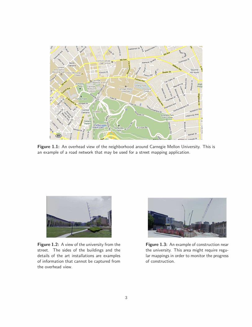
Figure 1.1: An overhead view of the neighborhood around Carnegie Mellon University. This isan example of a road network that may be used for a street mapping application.

Figure 1.2: A view of the university from thestreet. The sides of the buildings and thedetails of the art installations are examplesof information that cannot be captured fromthe overhead view.

Figure 1.3: An example of construction nearthe university. This area might require regu-lar mappings in order to monitor the progressof construction.

3

1.1.1 Mapping

The task of mapping is an important and well-studied problem in the field of robotics. Mapping

refers to traveling around a space in order to create a diagram or blueprint of the space. In

this work, we assume that a prior map is already available. The mapping problem becomes

a map updating problem where the goal is to maintain the freshness of information about the

environment. As differences arise between the environment and the prior map during online

traversal, fast replanning of a new route through the space is essential.

One mapping task, street mapping, has recently gained a lot of attention. For example, Figure

1.1 shows an overhead map of Carnegie Mellon University and the surrounding neighborhoods.

In order to build a visual map of the university from the viewpoint of the major roads around

the area, it is necessary to find an efficient way to traverse the roads and take pictures such as

those shown in Figures 1.2 and 1.3. In this scenario, the environment is a road network that

consists of both one-way and two-way streets. One-way streets commonly arise from the initial

map of the road networks, especially in urban settings. Additionally, dynamic factors such as

traffic or construction can change two-ways streets into one-way streets. On certain highways and

bridges, lanes can change from one direction to another depending on the time of day. Finally,

directionality constraints can occur as a result of the coverage goal. For example, in urban

street mapping, building occlusion makes capturing images of an area from a specific direction

important. If the prior map contains 3D points from one viewpoint, the coverage task may be

to capture images from other viewpoints to reconstruct the scene. These viewpoint restrictions

translate into directionality constraints for the coverage task.

Changes to the environment can occur without warning so it is important to update the map

and replan efficiently. In street mapping, the initial plan may be generated optimally offline.

However, during traversal, the map may be updated with changes such as introducing road

blockages, converting certain streets from two-way to one-way, or assigning a high traversability

cost to certain roads due to traffic. As these changes can occur online during traversal, an

algorithm with a low computation time is necessary in order to generate a new plan quickly and

continue the traversal with little delay.

Finally, using multiple robots allows the road network environment to be mapped more ef-

ficiently. By dividing the work among several robots, the total traversal time can be reduced.

Moreover, the use of more robots adds redundancy to the coverage solution if team members

become stuck in traffic or are delayed due to refueling. Finally, as more robots become available,

they can distribute the computation cost of generating a plan and reduce the total time spent

finding a solution.

1.1.2 Search

Search is an important component of many applications. For this work, we focus on search for

an object or objects that are generally static. In other words, the objects are not trying to evade

4

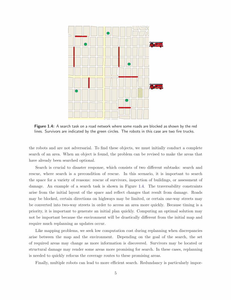
Figure 1.4: A search task on a road network where some roads are blocked as shown by the redlines. Survivors are indicated by the green circles. The robots in this case are two fire trucks.

the robots and are not adversarial. To find these objects, we must initially conduct a complete

search of an area. When an object is found, the problem can be revised to make the areas that

have already been searched optional.

Search is crucial to disaster response, which consists of two different subtasks: search and

rescue, where search is a precondition of rescue. In this scenario, it is important to search

the space for a variety of reasons: rescue of survivors, inspection of buildings, or assessment of

damage. An example of a search task is shown in Figure 1.4. The traversability constraints

arise from the initial layout of the space and reflect changes that result from damage. Roads

may be blocked, certain directions on highways may be limited, or certain one-way streets may

be converted into two-way streets in order to access an area more quickly. Because timing is a

priority, it is important to generate an initial plan quickly. Computing an optimal solution may

not be important because the environment will be drastically different from the initial map and

require much replanning as updates occur.

Like mapping problems, we seek low computation cost during replanning when discrepancies

arise between the map and the environment. Depending on the goal of the search, the set

of required areas may change as more information is discovered. Survivors may be located or

structural damage may render some areas more promising for search. In these cases, replanning

is needed to quickly refocus the coverage routes to these promising areas.

Finally, multiple robots can lead to more efficient search. Redundancy is particularly impor-

5

Figure 1.5: An example of a warehouse that requires regular patrols by a team of robots.

tant in disaster scenarios because the environment can be dangerous. Robots may get stuck or

be damaged by falling debris, for instance, and be unable to carry out the search. Therefore,

having more robots will increase the robustness of the team and ensure a complete search in spite

of unforeseen circumstances.

1.1.3 Patrol

Patrolling tasks seek a route through a space as a way to sweep the space and detect any unex-

pected changes. Patrolling is integral to security and surveillance problems where the environment

is expected to be relatively static, and any intrusions or discrepancies in the space need to be

reported. These tasks are also fairly routine jobs where the patrol is performed at regular inter-

vals throughout a period of time. Since the environment is fairly static, an efficient route can be

computed offline and then be used online.

An example is warehouse patrol, where a robot or team of robots is tasked with patrolling a

warehouse. A warehouse is a structured, bounded space that stores rows of objects separated into

aisles with corridors that connect each row as shown in Figure 1.5. Warehouses can sometimes

be divided into several floors. The patrol task is to check the storage facility to ensure nothing is

amiss.

Generally, warehouse patrols occur at night or when there is no activity in the space, i.e., no

work being done. While the environment is normally static throughout the length of the patrol,

it may change between patrol events. For example, if patrol sessions occur every night, objects in

the warehouse may have been moved, added, or removed during the daytime, rendering the map

from the previous night obsolete. As a result, the patrol route may need to be recomputed daily.

A team of robots can traverse a warehouse space more efficiently than a single robot can.

With a multi-floor warehouse, one robot or a pair of robots can be responsible for each floor. If

there is an intruder on the floor, the robots can signal to each other, and share this information.

When a robot fails or needs to go back to its charging station, other robots can take over its

share of the task.

6

Chapter 2

Problem Statement

This thesis addresses the problem of effective coverage of dynamic environments with incomplete

prior map information. For this problem, we strive for complete solutions while balancing com-

putation cost and solution quality. The environments we focus on are constrained, network-like

environments. As a result, they can be represented using a graph network. Additionally, the

following dimensions are included in the coverage problem we focus on in this thesis.

Partial Coverage: We define graph coverage or partial coverage as finding an Eulerian path

that visits all edges or a designated subset of the edges in the graph. Each edge has a cost

associated with it. The cost of a path is the sum of the costs of the edges that made up the path.

For this work, we seek a minimum cost Eulerian path for a graph.

Multiple Robots: We address the coverage problem for both single and multiple robots. With

multiple robots, the focus is on generating paths that are equivalent in cost. We follow a MinMax

objective where we strive to minimize the maximum cost path on the team.

Environmental Constraints: To make the algorithm more applicable to real-world problems,

we address environmental constraints in the form of travel restrictions in certain directions on

the graph. In this manner, we seek to minimize redundant traversals of each edge while respect-

ing its directionality. In the graph representation, the unrestricted or two-way connections are

undirected edges and the restricted or one-way connections are directed edges or arcs.

Replanning: Finally, during execution of the plan, the robot or robots may receive updates to

the graph prompting a replanning procedure. To achieve real-time operation, we aim for efficient

replanning techniques to handle online graph changes. We ensure that the new plans generated

for the robot or team of robots account for their current locations, which may be different from

their starting locations.

7

Assumptions

To bound the complexity of the problem, we make the following assumptions:

1. Perfect localization: We assume that changes detected by the navigation sensors are accurately

propagated into the map.

2. Perfect sensor readings: We do not model for sensor failures or incorrect readings.

3. Map representation: We assume that the environment is network-like so it can be represented

as a graph.

4. Assumptive planning: We assume the current map representation is an accurate reflection of

the environment. This belief holds until we detect discrepancies with our sensors. We also make

no assumptions about missing or incorrect map information.

5. Homogeneous teams: The types of the coverage problems are limited to teams of homogeneous

robots. Although these ideas can be applied to heterogeneous teams, we did not explicitly model

and test with those teams.

6. No robot interference: We do not explicitly plan for positions conflicts, i.e., when two or more

robots are at the same place at the same time. We assume this issue is handled by a lower level

planner during execution by adding delays to the plan.

Metrics

To evaluate the algorithms we present, we use the following metrics:

1. Path cost: The cost of the path or paths generated by the algorithms show the quality of the

solution.

2. Computation time: The time needed to compute the solution indicates the efficiency of the

approach, which is crucial for real-time operation.

3. Path cost variance: When evaluating the problem with multiple robots, the variance in the

cost of the paths reflects the balance of work between the robots. This translates to the total

traversal time for the team.

8

Chapter 3

Background and Related Work

The concept of covering a space has been explored extensively in the literature. We present

existing work from the areas of computer vision, path planning, and graph theory. We focus

on techniques in these areas that have been introduced for mapping, searching, and patrolling

applications. For each area, we describe how current approaches in the area relate to our thesis

problem in terms of the four problem dimensions: partial coverage, multiple robots, environmental

constraints, and replanning. Finally, we present a table comparing each of the approaches and

how well these approaches address the problem dimensions.

3.1 Model Construction

Model construction describes the problem of capturing information to construct a model or map

of the environment. This problem has been tackled in computer vision in the form of static

object construction and active sensing. These methods have been extended to robotics and used

for tasks such as mapping of unknown, dynamic 3D spaces.

3.1.1 Next Best View

In computer vision, an approach known as Next Best View finds the next camera placement

that will return the greatest amount of scene information. Since computing the information gain

from all points in the space is expensive, one of the Next Best View algorithms borrows from the

art gallery algorithm to randomly sample environment points from which to compute visibility

[Gonzalez-Banos, 2001]. This algorithm has been extended to a Next Best View approach used

to guide robots in mapping 3D indoor environments where the initial map is unknown [Gonzalez-

Banos and Latombe, 2002][Surmann et al., 2003]. While these methods can be applied to 3D

scenes, they rely on either 2D horizontal slices of the 3D model or 2D polygonal representations

which can be combined to create a 3D model. The visibility-based next view planning has been

used for only static environments.

9

Another set of Next Best View techniques uses occupancy grids as the model for assessing

information gain. Frontier-based planning methods threshold the occupancy probability to deter-

mine the next unvisited region [Yamauchi, 1997]. Frontiers are the known areas in the space that

border unknown regions. Stachniss and Burgard refine this idea by adding a belief probability

to each cell in the grid and choosing the next position as the closest cell with the lowest belief

probability [Stachniss and Burgard, 2003]. Other methods incorporate sensor geometry and speci-

fications to improve the reliability of obstacle detection [Grabowski et al., 2003] or to handle scene

occlusions [Maver and Bajcsy, 1993]. These planning methods present a more global approach

by searching over all locations in the environment rather than using only a sample location set.

As mentioned earlier, one of the early works in frontier search for multiple robots enabled

the robots to share an occupancy grid [Yamauchi, 1998]. However, the robots did not explicitly

coordinate their searches so multiple robots could potentially execute the same plan. The use of

multiple robots to ensure accurate localization while mapping the space has been addressed by

using the various robots to cover the region in a line pattern and stay close to one another in order

to estimate each other’s position [Rekleitis et al., 2000]. One work includes a bidding framework

between multiple robots for exploration and mapping as a way to maximize the information

gain [Simmons et al., 2000]. This work introduces a communication structure to coordinate the

exploration tasks. A simple bidding framework allows the robots to offer bids on the unknown

locations. A bid is a value that represents the estimated information gain and travel cost of a

particular robot to an unknown location in the space. A centralized agent collects these bids and

assigns the tasks using a greedy allocation algorithm. More recently, a fully distributed market-

based system has been used for multi-robot coordinaton that consists of an auctions [Zlot et al.,

2002]. In this system, the robots coordinate exploration by auctioning part of their work to the

other robots who bid on the auctioned task; the robot with the best bid wins. This approach

enables the robots to coordinate with each other using bids without relying on a centralized agent,

making this system more robust to communication failures.

3.1.2 Active Exploration

A related approach known as active exploration uses information-based methods to improve the

accuracy of the resulting map. One way to build more accurate maps is to use localization tech-

niques to minimize uncertainty [Bourgault et al., 2002]. Kollar and Roy leverage POMDPs to

learn optimal travel policies [Kollar and Roy, 2008]. While POMDPs provide optimal solutions,

they are computationally expensive for large problems. Hence, Kollar and Roy formulate the

problem as a reinforcement learning problem which enables more efficient computation. These

techniques mainly explore indoor environments where the scene is relatively static. Recent work

tackles the problem of dynamic indoor scenes. Hahnel et al. use learning techniques during map-

ping to detect dynamic objects such as people [Hahnel et al., 2003]. Biswas and Anguelov et al.

develop learned models of the dynamic objects using probabilistic representations [Biswas et al.,

10

2002][Anguelov et al., 2002]. Using the learned model, positions of certain objects in the environ-

ment can be determined at all times. However, for their experiments, the robot was stationary

and did not use the resulting maps for route planning.

The approaches for model construction focus on guiding robots to visit and build maps of unknown

spaces. These algorithms are efficient which is advantageous for replanning purposes even though

these algorithms do not explicitly address the issue of replanning. However, for our problem,

we assume a prior map is available and is fairly up-to-date. This allows us to start with more

information at the beginning of the problem which should lead to a more informed initial plan.

They also generally address open spaces unlike our focus on network-like spaces. Moreover, while

these approaches aim for completeness, they do not guarantee optimality or give bounds on the

solution quality. Finally, these algorithms do not address directionality constraints.

3.2 Continuous Coverage Planning

Continuous coverage is defined as finding a path through an open space such that the robot

passes a device over every part of the space. The navigation pattern employed depends mainly

on the range of the coverage device. The range of the device varies from robot-size devices to

infinite-size devices. These methods mainly operate on unknown, 2D and 3D spaces.

3.2.1 Robot-size Coverage Device

A robot-sized coverage device refers to an effector such as a mower or a floor cleaner. Solutions

to this set of continuous coverage problems first divide the map into cells and finds a path that

covers all the cells. The map division process is known as cellular decomposition. A survey

of these methods categorizes them into heuristic, approximate, semi-approximate, and exact

decompositions [Choset, 2001]. Template-based [Schmidt and Hofner, 1998][Liu et al., 2004]

methods belong to the heuristic category. The advantages of these methods are that they can

easily capture the vehicle characteristics in a set of motion parameters. However they are unable

to provide optimal coverage of a space.

Approximate cellular decompositions overlay a uniform grid over onto the space. One repre-

sentation model is a uniform rectangular grid. Techniques such as the wavefront algorithm [Zelin-

sky et al., 1993] and Spiral-STC [Gabriely and Rimon, 2002] give reasonable coverage results.

However, in complex worlds, these algorithm can result in redundant coverage. Additionally, the

Spanning Tree Coverage algorithm has been extended to multiple robots. The proposed algo-

rithms generate coverage routes through backtracking [Hazon and Kaminka, 2005] and minimize

the largest distance between every two robots [Agmon et al., 2006]. In this way, the coverage

paths can be spread out over the space. However, the total traversal time does not reduce pro-

11

portionally as the number of robots increases – the time for three or more robots may be the

same as the time for two robots. An improvement to this algorithm, known as Multi-robot Forest

Coverage [Zheng et al., 2005], generates a forest of trees that covers the environment where the

objective is to minimize the cost of the largest tree. The algorithm guarantees that its solution

cost is at most sixteen times the cost of the optimal solution. This algorithm performs better

than the multi-robot spanning tree coverage algorithm in finding routes that cover the space and

return the robots to their starting locations. A recent method, the Backtracking Spiral Algorithm

[Gonzalez et al., 2005], uses a spiral pattern to cover the grid. As the spirals proceed, backtrack-

ing points are collected and saved. These points are used to initialize other spirals for complete

coverage. An extension of the Backtracking Spiral Algorithm to multiple robots focuses on the

communication framework and negotiation strategies between the robots to visit unknown regions

of the space [Gonzalez and Gerlein, 2009]. Another representation model, triangular-based grid,

has been applied to cleaning robots [Oh et al., 2004]. This method generates smoother, more

efficient paths. Grid-based models perform poorly when the environment consists of nonpolygo-

nal objects since partially occluded cells are treated as obstacle cells. For complex environments,

there is a constant tradeoff between increasing cell resolution for more accurate coverage and

decreasing computation time for efficiency. Semi-approximate decompositions refine the uniform

grid by allowing parts of the cell to be any shape [Lumelsky et al., 1990], but still provide no

optimality guarantees.

Exact cellular decompositions use a segmentation method that accurately divides the space

into free or obstacle cells, allowing for complete coverage. A common exact cellular decomposition

divides a space into a set of trapezoids; each cell in the decomposition is then covered by up and

down motions. Boustrophedon decomposition decreases the number of map cells by combining

neighboring cells [Choset, 2000]. Another method, Morse decomposition, divides the space by

calculating critical points and operates using a few task-based coverage patterns [Acar et al.,

2002]. This approach also works incrementally to build the map in unknown environments. The

exact cellular decomposition technique has been extended to multiple robots [Latimer et al.,

2002]. In their approach, the robots cover the environment in close formation. After detecting an

obstacle in the environment and consequently encountering a critical point, the robot team splits

into subteams that investigate each region separated by the obstacle. The subteams merge when

they meet up with each other and continue traversing the space together. In this manner, a team

of robots can cover the environment more efficiently than a single robot. However it requires a

high level of communication and coordination.

3.2.2 Infinite-size Coverage Device

While most robotic devices have finite range, in certain cluttered spaces, they can be modeled

as infinite range devices. In this class, the coverage visibility of the vehicle is constrained by

the environment. A common approach for large footprint problems is path planning using the

12

generalized Voronoi diagram (GVD). The GVD is a roadmap for an environment where the road

stays equidistant from all obstacles and boundaries. This roadmap enables the robot to completely

cover the space. The hierarchical generalized Voronoi graph (HGVG) is an extension of the

GVD that operates in higher dimensions [Choset and Burdick, 2000]. An incremental version

of the HGVG has also been developed which enables coverage of an unknown space [Choset

et al., 2000]. Recent work in this area address the problem of building Voronoi regions in non-

convex environments with multiple robots [Breitenmoser et al., 2010]. By using a decentralized

framework using virtual targets and robot locations to build the Voronoi model, this work allows

for a better division of the environment among multiple robots.

3.2.3 Extended-range Coverage Device

For extended range devices where the detector range is greater than the robot but of finite mag-

nitude, Acar et al. present a hybrid approach called the hierarchical decomposition that combines

Morse decompositions and GVDs [Acar et al., 2006]. First, the environment is divided into re-

gions and each region assigned a label of either vast or narrow space. Vast spaces refer to regions

where the space is greater than the detector range and narrow spaces refer to regions where the

space is smaller than the detector range. Vast spaces can be covered using Morse decompositions

while narrow spaces are covered using a GVD. This incremental method provides complete cov-

erage, but makes no guarantees about optimality.

Most of the existing work in the continuous coverage planning present algorithms that guarantee

completeness of the entire space, but do not consider partial coverage or efficient replanning.

Since these techniques are intended for the coverage of open spaces, they may not work well for

the graph-like environments that we want to address. Finally, environmental constraints are not

considered in these approaches.

3.3 Comparison of Existing Work

Table 3.1 shows a comparison of the related work we just described and how well they address

each of the problem aspects.

So far, the algorithms discussed have been in robotics research which is the area in which this

thesis resides. However, while the approaches in model construction and open space coverage

13

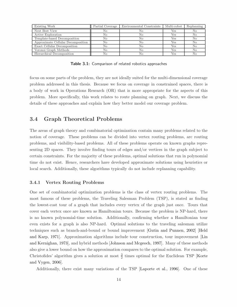
Existing Work Partial Coverage Environmental Constraints Multi-robot Replanning

Next Best View No No Yes NoActive Exploration No No Yes NoTemplate-based Decomposition No No Yes NoApproximate Cellular Decomposition No No Yes NoExact Cellular Decomposition No No Yes NoVoronoi Graph Methods No No Yes NoHierarchical Decomposition No No Yes No

Table 3.1: Comparison of related robotics approaches

focus on some parts of the problem, they are not ideally suited for the multi-dimensional coverage

problem addressed in this thesis. Because we focus on coverage in constrained spaces, there is

a body of work in Operations Research (OR) that is more appropriate for the aspects of this

problem. More specifically, this work relates to route planning on graph. Next, we discuss the

details of these approaches and explain how they better model our coverage problem.

3.4 Graph Theoretical Problems

The areas of graph theory and combinatorial optimization contain many problems related to the

notion of coverage. These problems can be divided into vertex routing problems, arc routing

problems, and visibility-based problems. All of these problems operate on known graphs repre-

senting 2D spaces. They involve finding tours of edges and/or vertices in the graph subject to

certain constraints. For the majority of these problems, optimal solutions that run in polynomial

time do not exist. Hence, researchers have developed approximate solutions using heuristics or

local search. Additionally, these algorithms typically do not include replanning capability.

3.4.1 Vertex Routing Problems

One set of combinatorial optimization problems is the class of vertex routing problems. The

most famous of these problems, the Traveling Salesman Problem (TSP), is stated as finding

the lowest-cost tour of a graph that includes every vertex of the graph just once. Tours that

cover each vertex once are known as Hamiltonian tours. Because the problem is NP-hard, there

is no known polynomial-time solution. Additionally, confirming whether a Hamiltonian tour

even exists for a graph is also NP-hard. Optimal solutions to the traveling salesman utilize

techniques such as branch-and-bound or bound improvement [Gutin and Punnen, 2002] [Held

and Karp, 1971]. Approximation algorithms include tour construction, tour improvement [Lin

and Kernighan, 1973], and hybrid methods [Johnson and Mcgeoch, 1997]. Many of these methods

also give a lower bound on how the approximation compares to the optimal solution. For example,

Christofides’ algorithm gives a solution at most 32 times optimal for the Euclidean TSP [Korte

and Vygen, 2006].

Additionally, there exist many variations of the TSP [Laporte et al., 1996]. One of these

14

variations, the Generalized TSP (G-TSP), clusters the vertices into neighborhoods and seeks a

tour that includes one point from each neighborhood. This problem can be reduced to a TSP

but with modified distances between the vertex pairs [Dimitrijevic and Saric, 1997]. Unlike the

TSP, the G-TSP is not only NP-hard, but all constant factor approximations are also NP-hard

[Safra and Schwartz, 2006]. In essence, the G-TSP requires running a TSP on all combinations

of vertices where each vertex resides in a different cluster.

An extension of the Traveling Salesman Problem to multiple robots is the k-Traveling Sales-

man Problem (k-TSP). The k-TSP seeks to find an optimal solution for k vehicles such that each

vertex in the graph is visited exactly once and the total cost of the k paths is minimized. The

k-TSP is NP-hard since it is a higher complexity version of the regular TSP, when k equals one.

Many exact algorithms have been proposed for the k-TSP, either as linear programming formu-

lation, or transformations to the TSP, as well as heuristics; many of them have been detailed in

a survey [Bektas, 2006].

Another version of the k-TSP with a different objective function is the Min Max k-TSP,

where the goal is to minimize the maximum cost path. Because the path cost is proportional

to time, the goal of this problem is to minimize the overall traversal time. Similar to the k-

TSP, it is NP-hard since it contains the TSP as a special case of k equals to one. An heuristic

algorithm for this problem was proposed that gave (52 −1k)-factor approximation on the optimal

solution [Frederickson et al., 1976a]. Additionally, in more recent work, there is an exact algorithm

and tabu search heuristic for algorithm [Franca et al., 1995].

While most research on routing problems focuses on static environments, some work addresses

dynamic graphs. The Dynamic Traveling Salesman Problem (DTSP) was introduced by Psaraftis

as part of dynamic vehicle routing problems. Recent work by Zhou et al. and Guntsch et al. uses

evolutionary methods to find approximate solutions to the DTSP [Zhou et al., 2003][Guntsch

et al., 2001]. Both approaches assume the changes rendered onto the graph are gradual, meaning

the number and location of vertices in the graph remain relatively constant.

While these algorithms do model the dimensions of our problem, they are more suited to

visiting specific areas of the space that are relatively sparse. However, the goal of our problem

is to visit all or most of the space. As a result, these vertex routing problems are not accurate

representations of our coverage problem.

3.4.2 Art Gallery and Watchman Problems

Another group of graph theoretic problems include the visibility-based art gallery problems and

the watchman problems. The art gallery problem, introduced by Victor Klee, is the problem

of finding the minimum number of guards that can maintain complete visibility of a polygonal

space, such as an art gallery. While polygonal algorithms exist that give an upper bound on the

number of guards that sufficiently cover a 2D polygonal space, finding the minimum number of

guards is NP-hard [Lee and Lin, 1986]. Greedy algorithms, such as [Amit et al., 2007], offer

15

heuristic-based approximate solutions that iteratively add to and prune a candidate guard set

while other sampling methods [Efrat and Har-Peled, 2006] randomly select a set of guard loca-

tions. The watchman problem similarly seeks to find the optimal route that a single guard can

travel to completely cover a space. Dror et al. introduce a O(n3logn) solution for a variation of

the watchman problem in a convex polygonal environment where the starting point is fixed [Dror

et al., 2003]. Using this solution, Tan infers a O(n4logn) exact algorithm for the general watch-

man problem [Tan, 2007] where the starting point is not fixed. Additionally, Tan presents an

approximation algorithm that gives good guarantees while maintaining a close-to-linear running

time for a simple polygon [Tan, 2007].

While these algorithms are good for finding the ideal locations or exact number of robots

to use for tasks with multiple robots, they do not account for partial coverage of the space.

Moreover, they do not take directionality constraints into consideration.

3.4.3 Arc Routing Problems

The set of combinatorial optimization problems that is the closest to our problem is the class of

arc routing problems. Arc routing problems generally seek an Eulerian tour, which is a path that

covers each edge once and begins and ends at the same vertex in the graph. Deciding whether

an Eulerian tour exists is solvable in polynomial time. For different types of graphs, the Eulerian

criterion changes depending on the kinds of edges in the graph. Edges in the graph can either be

directed or undirected. Throughout this thesis, the directed edges in a graph will be called arcs

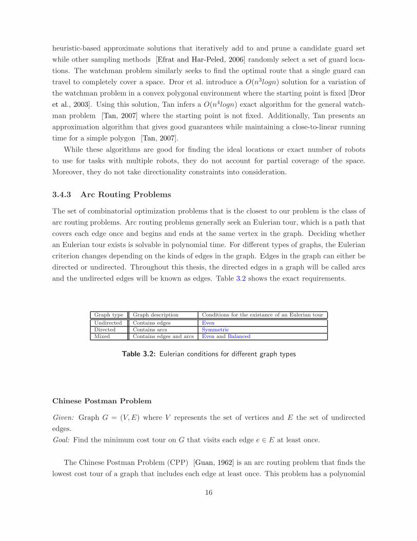
and the undirected edges will be known as edges. Table 3.2 shows the exact requirements.

Graph type Graph description Conditions for the existance of an Eulerian tour

Undirected Contains edges EvenDirected Contains arcs SymmetricMixed Contains edges and arcs Even and Balanced

Table 3.2: Eulerian conditions for different graph types

Chinese Postman Problem

Given: Graph G = (V,E) where V represents the set of vertices and E the set of undirected

edges.

Goal: Find the minimum cost tour on G that visits each edge e ∈ E at least once.

The Chinese Postman Problem (CPP) [Guan, 1962] is an arc routing problem that finds the

lowest cost tour of a graph that includes each edge at least once. This problem has a polynomial

16

time solution and algorithms to solve to this problem are surveyed in [Eiselt et al., 1995a]. From

Table 3.2, the criterion for an undirected graph to be Eulerian is for the degree of every vertex in

the graph to be even. We describe a general CPP algorithm. The first step is to determine the odd

degree vertices in the graph. Next, using a weighted matching algorithm, a minimum matching

is found over the set of odd degree vertices. A minimum weighted matching is a minimum

cost group of edges where the endpoints of the edges comprise the vertex set. This matching is

added to the graph as redundant edges. This graph addition essentially transforms the odd degree

vertices to even degree. Finally, a tour is created using the End-Pairing algorithm [Edmonds and

Johnson, 1973]. The next chapter contains more details of this algorithm. The CPP works well

for applications where it is necessary to traverse every part of the space. For example, Sorensen

uses the CPP to plan tours for farming machines in static known environments [Sorensen et al.,

2004]. Recently, this algorithm has been applied to open space coverage. Using a Boustrophedon

decomposition of the space, the order in which the cells are visited can be cast as a CPP. Using

the optimal cell order, the robot visits each cell in the CPP solution, and covers each cell in a

back and forth motion [Mannadiar and Rekleitis, 2010].

Rural Postman Problem

Given: Graph G = (V,ER ⊂ E) where V represents the set of vertices, E the set of undirected

edges, and ER is the required set of edges.

Goal: Find the minimum cost tour on G that visits each edge e ∈ ER at least once.

In many practical problems, it is not necessary to traverse all the edges in the graph. A routing

problem, the Rural Postman Problem (RPP), seeks a tour that traverses a required subset of the

graph edges using the remaining edges as travel links. Unlike the CPP, the RPP is a NP-hard

problem. Optimal solutions exist that formulate the RPP as an integer linear program and solve

it using branch-and-bound; many different formulations have been proposed for this problem as

surveyed in [Eiselt et al., 1995b]. Many TSP heuristics can be extended to the RPP [Laporte,

1997]. For example, Christofides’ approximation for the Euclidean TSP was modified for the

undirected RPP and maintains its 32 constant factor performance [Frederickson, 1979][Eiselt

et al., 1995b]. For arc routing problems, Moreira et al. present a heuristic-based approach for the

Dynamic Rural Postman Problem (DRPP) [Moreira et al., 2007]. They frame the problem as a

machine cutting application where the graph changes as pieces of the cutting surface are cut and

removed. Their approach uses visibility information to determine cut paths. Recently, the RPP

algorithm has been applied to the task of spray forming objects in automotive manufacturing

[Tewolde and Sheng, 2008]. The authors present two heuristic algorithms to solve this problem

efficiently.

17

Mixed Chinese Postman Problem

Given: Graph G = (V,E,A) where V represents the set of vertices, E the set of undirected edges,

and A is the set of arcs.

Goal: Find the minimum cost tour on G that visits each edge e ∈ E and each arc a ∈ A at least

once.

When there exist edge constraints in the graph, then the graph becomes a mixed graph

consisting of undirected edges and arcs. The problem of finding a single path that visits all edges

and arcs of a mixed graphs is known as the Mixed Chinese Postman Problem (MCPP). Related

work on this NP-hard problem includes both optimal and heuristic algorithms as summarized

in [Eiselt et al., 1995a]. Optimal techniques consist of either linear programming techniques

that solve the problem in a branch-and-bound fashion such as [Christofides et al., 1984][Win,

1992] or find a solution by a constraint relaxation approach to find the best solution [Nobert

and Picard, 1996]. Approximation algorithms consist of a algorithm introduced by Frederickson

[Frederickson, 1979] that returns a solution guaranteed to be at least 53 times the optimal solution.

Their algorithm consists of running two methods: one where the graph is first made even and

then symmetric, and second where the graph is first made symmetric, and then made even. Since

both methods do better in some cases and worse in others, both methods are run, and the lower

cost solution is returned. This algorithm was improved to give a 32 -factor approximation through

a change in one of the two methods [Raghavachari and Veerasamy, 1998].

Mixed Rural Postman Problem

Given: Graph G = (V,ER ⊂ E,AR ⊂ A) where V represents the set of vertices, E the set of

undirected edges, A is the set of arcs, and ER and AR are the sets of required edges and arcs,

respectively.

Goal: Find the minimum cost tour on G that visits each edge e ∈ ER and each arc a ∈ AR at

least once.

For our work, we focus on a general version of the MCPP known as the Mixed Rural Post-

man Problem (MRPP) where it is necessary to visit only a subset of the edges and arcs of the

graph. In previous work, this problem has been addressed by transforming and solving it as other

NP-hard problems such as the Mixed General Routing Problem [Corberan et al., 2005] and the

Asymmetric TSP [Laporte, 1997] . Additionally, one set of approximation algorithms have been

introduced [Corberan et al., 2000] that consist of a constructive heuristic and a tabu method that

refines the solution. While the constructive heuristic is computationally inexpensive, it does not

provide solutions that are as high in quality as the tabu method (which can produce near-optimal

solutions at a much higher computation cost). One related problem to the MRPP is the Windy

Rural Postman Problem (WRPP) which seeks a route for an undirected graph where the cost of

18

each edge changes depending on the direction of traversal. This problem contains the Undirected

Rural Postman problem, Directed Rural Postman problem, and Mixed Rural Postman problem as

special cases. A set of constructive heuristics and improvement procedures has been proposed for

this [Benavent et al., 2003] with results where the average difference between the approximation

solution and the lower bound on the optimal solution is 4%. These heuristics and procedures have

been improved and combined with a multi-start algorithm within a scatter search framework to

further decrease the amount of deviation from the optimal solution to 1.75% [Benavent et al.,

2005].

For multiple robots, there are extensions of the single robot arc routing problems on undirected

graphs: k-Chinese Postman Problem and k-Rural Postman Problem. For mixed graphs, these

problems are the k-Mixed Chinese Postman Problem and the k-Mixed Rural Postman Problem.

k-Chinese Postman Problem

Given: Graph G = (V,E) where V represents the set of vertices, E the set of undirected edges,

and k robots.

Goal: Find the set of k tours on G that in total visit each edge e ∈ E such that the cost of the

maximum cost tour is minimized.

Two versions of the k-Chinese Postman Problem (k-CPP) exist: one is a direct extension

of the CPP where the objective is to minimize the sum of the k tour lengths. Polynomial

algorithms [Assad et al., 1987][Zhang, 1992] exist that produce optimal solutions to this problem.

However, for many practical applications, optimizing the total tour length may not be ideal since

the optimal solution may assign one robot to do all the work. A second version of the k-CPP

is known as the Min Max k-CPP (MM k-CPP), where the goal is to minimize the maximum

length path as a way to reduce the total time spent and to equalize the work among the k

robots. The MM k-CPP is NP-hard. While an optimal solution does exist [Ahr, 2004], it is not

computationally efficient enough for practical problems. As a result, a number of heuristics have

been developed to provide more efficient solutions to the MM k-CPP problem [Frederickson et al.,

1976b][Ahr and Reinelt, 2002][Ahr and Reinelt, 2006].

k-Rural Postman Problem

Given: Graph G = (V,ER ⊂ E) where V represents the set of vertices, E the set of undirected

edges, ER the set of required edges and k robots.

Goal: Find the set of k tours on G that in total visit each edge e ∈ ER such that the cost of the

maximum cost tour is minimized.

19

The RPP is extended to multiple robots in the form of the k-Rural Postman Problem (k-

RPP). To our knowledge, only one algorithm exists for the k-RPP. The algorithm is a heuristic

algorithm introduced by Easton and Burdick [Easton and Burdick, 2005]. The k-RPP algorithm

consists of two main parts: clustering the graph into k sections using the farthest-point clustering

algorithm [Gonzalez, 1985] and finding a route for each cluster with the spanning tree and CPP

algorithms. The k robots are assumed to start from the same depot. This approach has been

extended to dynamic settings where the graph and number of robots can change [Williams and

Burdick, 2006].

k-Mixed Chinese Postman Problem and k-Mixed Rural Postman Problem

k-MCPP

Given: Graph G = (V,E,A) where V represents the set of vertices, E the set of undirected edges,

A the set of arcs, and k robots.

Goal: Find the set of k tours on G that in total visit each edge e ∈ E and a ∈ A such that the

cost of the maximum cost tour is minimized.

k-MRPP

Given: Graph G = (V,ER ⊂ E,AR ⊂ A) where V represents the set of vertices, E the set of

undirected edges, A is the set of arcs, and ER and AR are the sets of required edges and arcs,

respectively and k robots.

Goal: Find the set of k tours on G that in total visit each edge e ∈ ER and each arc a ∈ AR such

that the cost of the maximum cost tour is minimized.

In many applications, it is common to have multiple robots working together to complete

a task. In these cases, the above problems become the k-Mixed Chinese Postman Problem (k-

MCPP) and the k-Mixed Rural Postman Problem (k-MRPP) where k is the number of robots.

We clarify that we are focused on the Min Max versions of these problems, meaning that we

want to minimize the maximum path cost. To our knowledge, there have been no algorithms

that specifically address the k-MCPP and the k-MRPP. A related problem, the k-Windy Rural

Postman problem has an optimal algorithm [Benavent et al., 2009] which can be applied to these

two problems, but the optimal approach is not suitable for applications where computation time

is limited. Since the k-MCPP is a special case of the k-MRPP (when there are no optional edges),

we will focus on the k-MRPP in this work since any solution to it can directly be applied to the

k-MCPP.

Table 3.3 shows a comparison of the graph theoretical problems, how well they model each of

the problem dimensions, and whether there are existing algorithms for the problem.

20

Problem Partial Coverage Environmental Constraints Multiple robots Replanning Existing work

CPP No No No No YesRPP Yes No No No YesMCPP No Yes No No YesMRPP Yes Yes No No Yesk-CPP No No Yes No Yesk-RPP Yes No Yes No Yesk-MCPP No Yes Yes No Nok-MRPP Yes Yes Yes No No

Table 3.3: Comparison of graph theoretical problems

For environmental coverage with robots, it is important to replan efficiently in order to gen-

erate new routes as the map is updated when new information is discovered. However, this is

not a consideration for operations research algorithms, so an important goal of this thesis is to

use these arc routing problems to model the coverage problem, and find solution approaches that

are both effective in completing the task and computationally efficient for replanning on robotics

tasks.

3.5 Approach

Our approach focuses on an integrated framework that strives for complete solutions to the cov-

erage problem by using lower complexity algorithms to approximate solutions to higher

complexity problems. Environmental restrictions in the form of directionality constraints

are incorporated into the framework. While this framework can generate optimal solutions to

specific cases of the coverage problem, it provides approximate solutions for the general

problem where the lower complexity algorithm is computationally expensive. The

extension of the approach to multiple robots uses a two-fold technique, which consists of

a routing step and a clustering step. Finally, efficient replanning is achieved through ad-

ditions to the model and incorporating preventative heuristics during plan building.

Because computation time for replanning can be considerable in these cases, we aim for a dy-

namic approach that seeks optimal solutions if time permits and heuristic solutions

to provide real-time computation.

21

22

Chapter 4

Partial Coverage with a Single Robot

without Environmental Constraints

The first problem that we address is the single robot coverage problem, where coverage can be

partial and replanning is important. While this problem is missing two dimensions (environmental

constraints and multiple robots) of the general coverage problem, it is still important for many

tasks. Street mapping tasks that operate on road networks without directionality constraints

occur in many suburban areas and on major roads and highways. In disaster response, debris

may block a corridor and obscure it from both sides rather than from just one side. Finally, in

warehouse patrolling, there are generally no limitations on the direction of travel in the aisles of

the building. For all three of these tasks, it is not necessary to use more than one robot. However,

replanning is crucial for these tasks since changes can always occur in the environment.

The problem of partial coverage with a single robot is the least complex of the problems

we are addressing. Therefore we focus on finding an optimal solution that is computationally

efficient and suitable for real-time operation. In a graph representation, this problem can be cast

as the Rural Postman problem for which the Chinese Postman problem is a special case. Both

optimal and heuristic algorithms exist for this problem. While these approaches work for a range

of Rural Postman problems with any combination of optional and required edges, we focus on

graphs where the set of optional edges is relatively small (meaning that the problem is a slightly

deviation from the Chinese Postman problem). We present a path building strategy with the goal

of maintaining or minimizing the size of the optional edge set. In this chapter, we describe both

the Chinese Postman and Rural Postman problems, explain our optimal algorithm and heuristic

for the Rural Postman problem, show results from tests, and discuss our approach. Finally, we

present a method that parallelizes the Rural Postman algorithm among multiple processes and

show how this strategy improves computational efficiency.

23

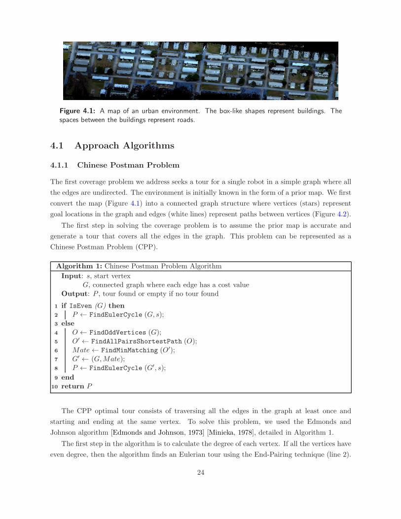
Figure 4.1: A map of an urban environment. The box-like shapes represent buildings. Thespaces between the buildings represent roads.

4.1 Approach Algorithms

4.1.1 Chinese Postman Problem

The first coverage problem we address seeks a tour for a single robot in a simple graph where all

the edges are undirected. The environment is initially known in the form of a prior map. We first

convert the map (Figure 4.1) into a connected graph structure where vertices (stars) represent

goal locations in the graph and edges (white lines) represent paths between vertices (Figure 4.2).

The first step in solving the coverage problem is to assume the prior map is accurate and

generate a tour that covers all the edges in the graph. This problem can be represented as a

Chinese Postman Problem (CPP).

Algorithm 1: Chinese Postman Problem Algorithm

Input: s, start vertexG, connected graph where each edge has a cost value

Output: P , tour found or empty if no tour found

1 if IsEven (G) then2 P ← FindEulerCycle (G, s);3 else4 O ← FindOddVertices (G);5 O′ ← FindAllPairsShortestPath (O);6 Mate← FindMinMatching (O′);7 G′ ← (G,Mate);8 P ← FindEulerCycle (G′, s);

9 end10 return P

The CPP optimal tour consists of traversing all the edges in the graph at least once and

starting and ending at the same vertex. To solve this problem, we used the Edmonds and

Johnson algorithm [Edmonds and Johnson, 1973] [Minieka, 1978], detailed in Algorithm 1.

The first step in the algorithm is to calculate the degree of each vertex. If all the vertices have

even degree, then the algorithm finds an Eulerian tour using the End-Pairing technique (line 2).

24

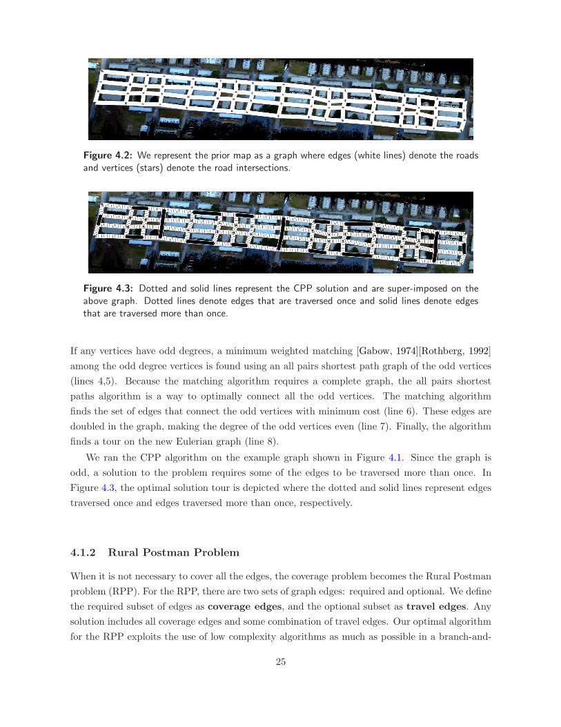
Figure 4.2: We represent the prior map as a graph where edges (white lines) denote the roadsand vertices (stars) denote the road intersections.

Figure 4.3: Dotted and solid lines represent the CPP solution and are super-imposed on theabove graph. Dotted lines denote edges that are traversed once and solid lines denote edgesthat are traversed more than once.

If any vertices have odd degrees, a minimum weighted matching [Gabow, 1974][Rothberg, 1992]

among the odd degree vertices is found using an all pairs shortest path graph of the odd vertices

(lines 4,5). Because the matching algorithm requires a complete graph, the all pairs shortest

paths algorithm is a way to optimally connect all the odd vertices. The matching algorithm

finds the set of edges that connect the odd vertices with minimum cost (line 6). These edges are

doubled in the graph, making the degree of the odd vertices even (line 7). Finally, the algorithm

finds a tour on the new Eulerian graph (line 8).

We ran the CPP algorithm on the example graph shown in Figure 4.1. Since the graph is

odd, a solution to the problem requires some of the edges to be traversed more than once. In

Figure 4.3, the optimal solution tour is depicted where the dotted and solid lines represent edges

traversed once and edges traversed more than once, respectively.

4.1.2 Rural Postman Problem

When it is not necessary to cover all the edges, the coverage problem becomes the Rural Postman

problem (RPP). For the RPP, there are two sets of graph edges: required and optional. We define

the required subset of edges as coverage edges, and the optional subset as travel edges. Any

solution includes all coverage edges and some combination of travel edges. Our optimal algorithm

for the RPP exploits the use of low complexity algorithms as much as possible in a branch-and-

25

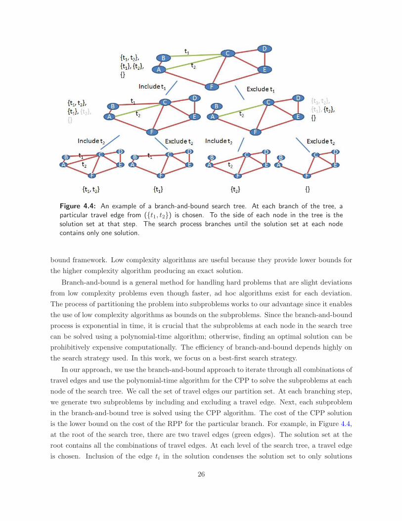
Figure 4.4: An example of a branch-and-bound search tree. At each branch of the tree, aparticular travel edge from ({t1, t2}) is chosen. To the side of each node in the tree is thesolution set at that step. The search process branches until the solution set at each nodecontains only one solution.

bound framework. Low complexity algorithms are useful because they provide lower bounds for

the higher complexity algorithm producing an exact solution.

Branch-and-bound is a general method for handling hard problems that are slight deviations

from low complexity problems even though faster, ad hoc algorithms exist for each deviation.

The process of partitioning the problem into subproblems works to our advantage since it enables

the use of low complexity algorithms as bounds on the subproblems. Since the branch-and-bound

process is exponential in time, it is crucial that the subproblems at each node in the search tree

can be solved using a polynomial-time algorithm; otherwise, finding an optimal solution can be

prohibitively expensive computationally. The efficiency of branch-and-bound depends highly on

the search strategy used. In this work, we focus on a best-first search strategy.

In our approach, we use the branch-and-bound approach to iterate through all combinations of

travel edges and use the polynomial-time algorithm for the CPP to solve the subproblems at each

node of the search tree. We call the set of travel edges our partition set. At each branching step,

we generate two subproblems by including and excluding a travel edge. Next, each subproblem

in the branch-and-bound tree is solved using the CPP algorithm. The cost of the CPP solution

is the lower bound on the cost of the RPP for the particular branch. For example, in Figure 4.4,

at the root of the search tree, there are two travel edges (green edges). The solution set at the

root contains all the combinations of travel edges. At each level of the search tree, a travel edge

is chosen. Inclusion of the edge ti in the solution condenses the solution set to only solutions

26

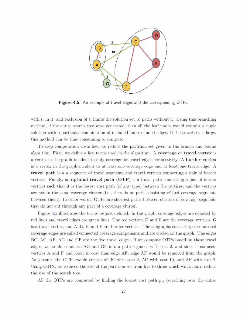
Figure 4.5: An example of travel edges and the corresponding OTPs.

with ti in it, and exclusion of ti limits the solution set to paths without ti. Using this branching

method, if the entire search tree were generated, then all the leaf nodes would contain a single

solution with a particular combination of included and excluded edges. If the travel set is large,

this method can be time consuming to compute.

To keep computation costs low, we reduce the partition set given to the branch and bound

algorithm. First, we define a few terms used in the algorithm. A coverage or travel vertex is

a vertex in the graph incident to only coverage or travel edges, respectively. A border vertex

is a vertex in the graph incident to at least one coverage edge and at least one travel edge. A

travel path is a a sequence of travel segments and travel vertices connecting a pair of border

vertices. Finally, an optimal travel path (OTP) is a travel path connecting a pair of border

vertices such that it is the lowest cost path (of any type) between the vertices, and the vertices

are not in the same coverage cluster (i.e., there is no path consisting of just coverage segments

between them). In other words, OTPs are shortest paths between clusters of coverage segments

that do not cut through any part of a coverage cluster.

Figure 4.5 illustrates the terms we just defined. In the graph, coverage edges are denoted by

red lines and travel edges are green lines. The red vertices D and E are the coverage vertices, G

is a travel vertex, and A, B, E, and F are border vertices. The subgraphs consisting of connected

coverage edges are called connected coverage components and are circled on the graph. The edges

BC, AC, AF, AG and GF are the five travel edges. If we compute OTPs based on these travel

edges, we would condense AG and GF into a path segment with cost 2, and since it connects

vertices A and F and lower in cost than edge AF, edge AF would be removed from the graph.

As a result, the OTPs would consist of BC with cost 2, AC with cost 10, and AF with cost 2.

Using OTPs, we reduced the size of the partition set from five to three which will in turn reduce

the size of the search tree.

All the OTPs are computed by finding the lowest cost path pij (searching over the entire

27

graph) between each pair of border vertices vi and vj in different clusters. If pij is a travel path,

we save it as an OTP. If pij is not a travel path, then vi and vj do not have an OTP between them

(i.e., pij = NULL). The OTPs become our partition set. The OTPs are unlabeled at the beginning

of the algorithm. We iterate through the OTP set within the branch-and-bound framework. At

each branch step, the algorithm generates a new subproblem by either including or excluding

an OTP. At the beginning of the RPP algorithm shown in Algorithm 2, we assign cost 0 to the

unlabeled OTPs and solve the problem with all the OTPs set as required edges using the CPP

algorithm (lines 2,3). The problem and CPP cost are pushed onto a priority queue (line 4). The

CPP cost is the lower bound on the problem since all the OTPs have zero cost. While the queue

is not empty, the lowest cost subproblem is selected from the queue (lines 5,6).

Algorithm 2: Rural Postman Problem Algorithm

Input: s, start vertexG = (C, T ), graph where each edge has a label and a cost value. C is the subset ofcoverage edges, and T is the subset of travel edgesOTP , subset of OTPs

Output: P , tour found or empty if no tour found

1 pq ← [];2 G′ ← [G,OTP ] where ∀pij ∈ OTP , cost(pij) = 03 P ← CPP (s,G′);4 pq.Push ([G′, P ]);5 while pq.Size () > 0 do6 [G′, P ]← pq.Pop ();7 pij ← FindMaxOTP (G′);8 if pij == [] then9 return P ;

10 end11 G1 ← IncludeEdge (G′, pij);12 P1← CPP (s,G1);13 pq.Push ([G1, P1]);14 G2 ← RemoveEdge (G′, pij);15 P2← CPP (s,G2);16 pq.Push ([G2, P2]);

17 end18 return [];

For the subproblem, the algorithm selects an unlabeled OTP pij with the highest path cost

(line 7). By employing this strategy of choosing the OTP with the highest path cost, our aim

is to increase the lower bound by the largest amount, which may help focus the search to the

correct branch and prevent extraneous explorations. Once an OTP pij is selected, two branches

are generated; the first branch includes pij in the solution (line 11), this time with the real path

cost assigned, and the second branch omits pij from the solution (line 14). A solution to each

28

branch is found using the CPP algorithm (lines 12,15). Because each solution is generated with

a cost of 0 assigned to the unlabeled OTPs in the subproblem, the costs of the inclusion and

exclusion CPP solutions represent lower bounds on the cost of the RPP with and without using

pij for travel, respectively. These new subproblems are added to the priority queue (lines 13, 16),

and the algorithm iterates until the lowest cost problem in the queue contains no OTPs (line 8).

The solution to this problem is the optimal solution to the RPP since it has either included or

excluded every single OTP, and has a path cost that is equal to or lower than the lower bounds

of the other branches. The branch-and-bound algorithm for the RPP is an exponential algorithm

with a complexity of O(|V |32t) where t is the number of OTPs and |V | is the number of vertices

in the graph.

Two additional improvements were made to the CPP algorithm to work with the RPP, shown

in Algorithm 3. The first permitted the use of travel edges as part of the shortest path segments

between the set of odd vertices. This allows the CPP to reason directly about the paths that cut

through coverage clusters. More specifically, while the partition set for the branch-and-bound

method consists only of OTPs, we retain some of the travel edges in the original graph. These

travel edges do not connect disjoint coverage components. They instead are edges that travel

between coverage vertices within a component. Having these extra travel edges allows the CPP

algorithm to use them as part of the matching. In this manner, these travel edges can enable

a lower cost set of doubled edges. As a result, in the modified CPP algorithm shown in line

5, the FindAllPairsShortestPath method is modified to include travel edges as part of the path

computation.

The second improvement to the CPP algorithm concerns the generation of Euler cycles. Since

the FindEulerCycle method can be expensive, we modified the CPP algorithm so the Eulerian

tour is generated only when necessary. When a solution graph is found (i.e., it contains no

OTPs), it is necessary to generate a path (lines 8 - 11). Otherwise, only a lower bound is needed

in order to progress the search during most of the branch-and-bound process. This lower bound

is computed by taking the sum of all the edge costs in the graph G′ where any OTPs have zero

cost, and all other edges, travel or coverage, retain their original costs (line 14).

This approach can be extended to the Directed Rural Postman problem (where the graph

contains only arcs). Since this problem is not as applicable as the undirected RPP to various

coverage problems, we discuss the details in the Appendix A.

4.1.3 Online Changes

Dynamic changes occur when the environment differs from the original map. As stated previously,

we choose to use lower-complexity assumptive planning in order to generate solutions quickly.

In our planner, an initial plan is found based on the graph of the environment. As the

vehicle uncovers differences between the map and environment during traversal, the algorithm

propagates them into the graph structure. This may require a simple graph modification such

29

Algorithm 3: Modified Chinese Postman Problem Algorithm

Input: s, start vertexG, connected graph where each edge has a cost value

Output: LB, P where LB is the cost of the graph path and P is tour found or empty ifno tour is found or if the graph still contains OTPs

1 if IsEven(G) then2 P ← FindEulerCycle (G, s);3 else4 O ← FindOddVertices (G);5 O′ ← FindAllPairsShortestPathUsingTravel (O);6 Mate← FindMinMatching (O′);7 G′ ← (G,Mate);8 if ContainsOTP (G) then9 P ← FindEulerCycle (G′, s);

10 LB ← SumPathCost (P );

11 end12 else13 P ← [];14 LB ← ComputeCost (G′);

15 end

16 end17 return LB,P ;

30

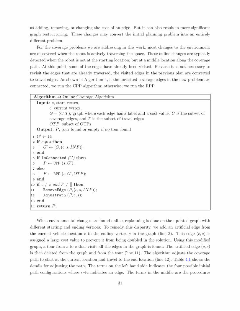
as adding, removing, or changing the cost of an edge. But it can also result in more significant

graph restructuring. These changes may convert the initial planning problem into an entirely

different problem.

For the coverage problems we are addressing in this work, most changes to the environment

are discovered when the robot is actively traversing the space. These online changes are typically

detected when the robot is not at the starting location, but at a middle location along the coverage

path. At this point, some of the edges have already been visited. Because it is not necessary to

revisit the edges that are already traversed, the visited edges in the previous plan are converted

to travel edges. As shown in Algorithm 4, if the unvisited coverage edges in the new problem are

connected, we run the CPP algorithm; otherwise, we run the RPP.

Algorithm 4: Online Coverage Algorithm

Input: s, start vertex,c, current vertex,G = (C, T ), graph where each edge has a label and a cost value. C is the subset ofcoverage edges, and T is the subset of travel edgesOTP , subset of OTPs

Output: P , tour found or empty if no tour found

1 G′ ← G;2 if c 6= s then3 G′ ← [G, (c, s, INF )];4 end5 if IsConnected (C) then6 P ← CPP (s,G′);7 else8 P ← RPP (s,G′, OTP );9 end

10 if c 6= s and P 6= [] then11 RemoveEdge (P, (c, s, INF ));12 AdjustPath (P, c, s);

13 end14 return P ;

When environmental changes are found online, replanning is done on the updated graph with

different starting and ending vertices. To remedy this disparity, we add an artificial edge from

the current vehicle location c to the ending vertex s in the graph (line 3). This edge (c, s) is

assigned a large cost value to prevent it from being doubled in the solution. Using this modified

graph, a tour from s to s that visits all the edges in the graph is found. The artificial edge (c, s)

is then deleted from the graph and from the tour (line 11). The algorithm adjusts the coverage

path to start at the current location and travel to the end location (line 12). Table 4.1 shows the

details for adjusting the path. The terms on the left hand side indicates the four possible initial

path configurations where s→c indicates an edge. The terms in the middle are the procedures

31

for adjusting the specific path, and the terms on the right are the final paths returned after the

adjustment method.

s...s→(c...s) ⇒ (c...s)→s...s ⇒ c...s...s(s...c)→s...s ⇒ Reverse(s...c)→s...s ⇒ c...s...ss→(c...s) ⇒ (c...s)→s ⇒ c...s(s...c)→s ⇒ Reverse(s...c)→s ⇒ c...s

Table 4.1: Path adjustment steps for the online coverage algorithm

We now step through an example that illustrates the online coverage algorithm. In Figure

4.3, a CPP solution of the example graph is shown. In Figure 4.9, the vehicle traverses the initial

CPP path until it discovers the third edge in its path is missing. The vehicle does not know about

this change until it reaches the previous edge. The algorithm then sets the traversed edges in the

path to be travel (Figure 4.10) and replans a new coverage tour shown in Figure 4.11. However,

it encounters another missing edge as it travels along the new path. The traversed edges in the

previous path are also converted to travel edges (Figure 4.12) and a final plan is found (Figure

4.13).

4.1.4 Farthest Distance Heuristic

In our algorithm, when a robot encounters a change at a particular vertex, these changes are

obstacles which prevent the robot from completing the current coverage solution. As a result, the

problem needs to be re-solved with the previously traversed edges converted to travel edges. The

number of optimal travel paths can be very large if the travel edges break the coverage subgraph

into a large number of connected components. Therefore, to maintain efficiency, we want to keep

the number of coverage components close to one. Ideally, we want the coverage subgraph and

travel subgraph to be mutually independent. This would ensure that the required subgraph is

connected, which is important for maintaining the coverage problem as a CPP, and maximize the

likelihood that when the next change is detected, the travel edges do not disconnect the coverage

components.

In the CPP algorithm, we use the End-Pairing technique (Algorithm 6) to generate the Eu-

lerian cycle from the graph. The algorithm consists of two steps. First, it builds cycles that

intersect at at least one vertex. Next, the cycles are merged together two at a time by adding

one cycle onto another at the intersecting vertex. The cycle building step is shown in Algorithm

5. During each step of the algorithm, edges are added to a path sequence and removed from the

graph until the starting vertex of the path is encountered. In the original End-Pairing algorithm,

the heuristic for choosing the next edge to add to the sequence consisted of picking a random

32

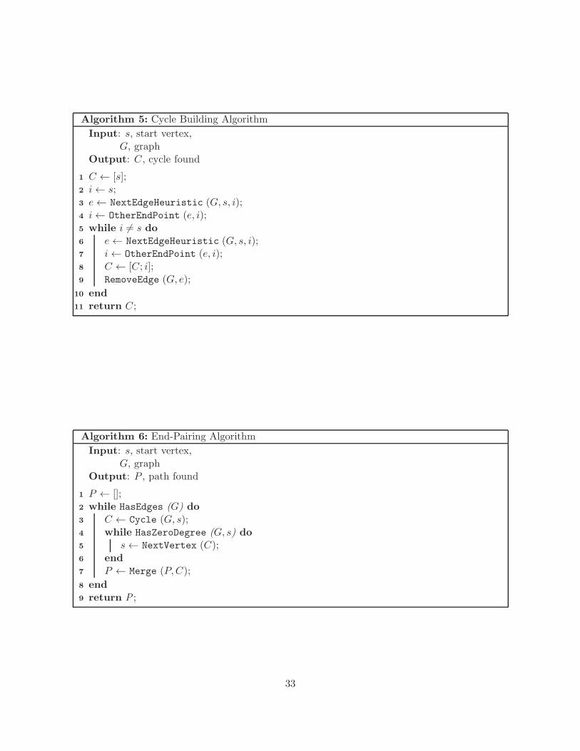
Algorithm 5: Cycle Building Algorithm

Input: s, start vertex,G, graph

Output: C, cycle found

1 C ← [s];2 i← s;3 e← NextEdgeHeuristic (G, s, i);4 i← OtherEndPoint (e, i);5 while i 6= s do6 e← NextEdgeHeuristic (G, s, i);7 i← OtherEndPoint (e, i);8 C ← [C; i];9 RemoveEdge (G, e);

10 end11 return C;

Algorithm 6: End-Pairing Algorithm

Input: s, start vertex,G, graph

Output: P , path found

1 P ← [];2 while HasEdges (G) do3 C ← Cycle (G, s);4 while HasZeroDegree (G, s) do5 s← NextVertex (C);6 end7 P ← Merge (P,C);

8 end9 return P ;

33

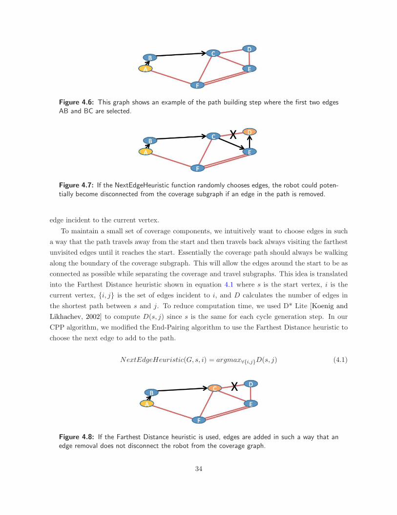
Figure 4.6: This graph shows an example of the path building step where the first two edgesAB and BC are selected.

Figure 4.7: If the NextEdgeHeuristic function randomly chooses edges, the robot could poten-tially become disconnected from the coverage subgraph if an edge in the path is removed.

edge incident to the current vertex.

To maintain a small set of coverage components, we intuitively want to choose edges in such

a way that the path travels away from the start and then travels back always visiting the farthest

unvisited edges until it reaches the start. Essentially the coverage path should always be walking

along the boundary of the coverage subgraph. This will allow the edges around the start to be as

connected as possible while separating the coverage and travel subgraphs. This idea is translated

into the Farthest Distance heuristic shown in equation 4.1 where s is the start vertex, i is the

current vertex, {i, j} is the set of edges incident to i, and D calculates the number of edges in

the shortest path between s and j. To reduce computation time, we used D* Lite [Koenig and

Likhachev, 2002] to compute D(s, j) since s is the same for each cycle generation step. In our

CPP algorithm, we modified the End-Pairing algorithm to use the Farthest Distance heuristic to

choose the next edge to add to the path.

NextEdgeHeuristic(G, s, i) = argmax∀{i,j}D(s, j) (4.1)

Figure 4.8: If the Farthest Distance heuristic is used, edges are added in such a way that anedge removal does not disconnect the robot from the coverage graph.

34

Figure 4.9: During traversal of the CPP solution, the robot discovers that the third edge inthe path is missing and ends the traversal. Dotted lines denote edges that are traversed onceand solid lines denote edges that are traversed more than once. The robot started out at theupper left corner of the graph.

Figure 4.10: To prevent visiting edges that have been already traversed, the graph is modifiedby setting the traversed edges to be travel edges, represented by green lines.

To illustrate the heuristic, we step through an example. In Figure 4.6, the graph is shown with

the starting location at vertex A. During the path building step, the NextEdgeHeuristic function

chooses edges AB and BC using either the Farthest Distance heuristic or the random heuristic. If

the random heuristic is used, then the function could potentially choose CE and ED as the next

edges. If during travel, CD is discovered to be blocked, then the vehicle would be at location D.

Since the visited edges would be converted into travel, vertex D would be disconnected from the

remaining coverage edges by the travel edges. However, if the Farthest Distance heuristic had

been used when the vehicle was at vertex C, CD would be the next edge chosen since D is the

farthest from the starting vertex. In this case if CD is found to be blocked, the vehicle would be

at vertex C and still be connected to the coverage edges.

4.2 Comparison Tests

Our testing compared the Farthest Distance heuristic against the original heuristic of randomly

selecting a neighboring edge as the next edge. For the tests, we vary four different parameters:

traversal heuristic, graph, starting vertex s, and set of changes. At the beginning of each test run,

the graph is connected and has no travel edges. Using the CPP algorithm, a tour is computed.

The test simulates a robot executing the tour starting at vertex s. If along the execution, the

next edge to be traversed is in the change set, that edge is considered blocked. It is removed

35

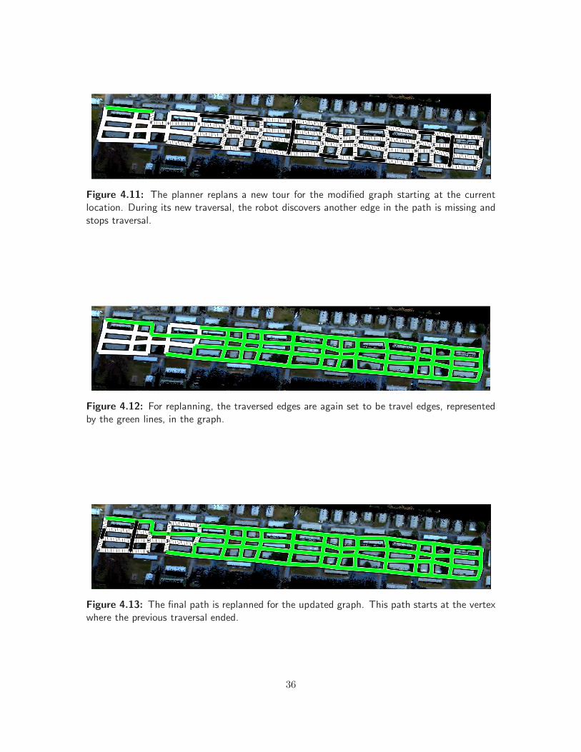
Figure 4.11: The planner replans a new tour for the modified graph starting at the currentlocation. During its new traversal, the robot discovers another edge in the path is missing andstops traversal.

Figure 4.12: For replanning, the traversed edges are again set to be travel edges, representedby the green lines, in the graph.

Figure 4.13: The final path is replanned for the updated graph. This path starts at the vertexwhere the previous traversal ended.

36

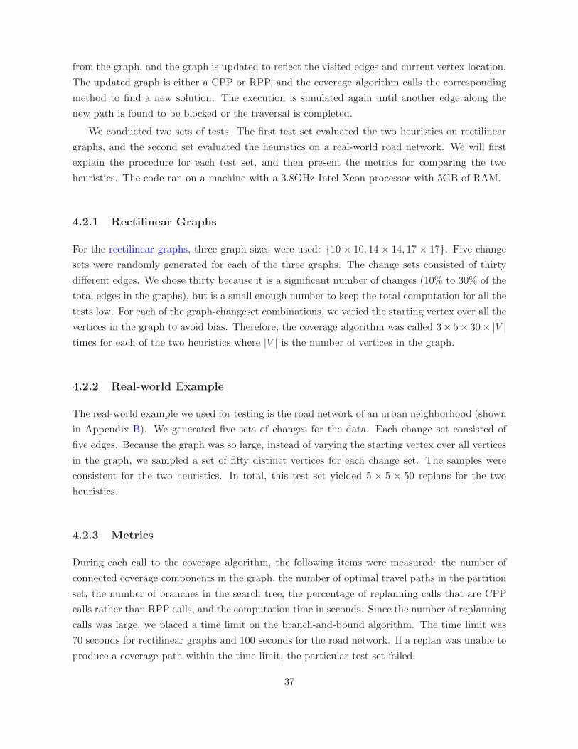
from the graph, and the graph is updated to reflect the visited edges and current vertex location.

The updated graph is either a CPP or RPP, and the coverage algorithm calls the corresponding

method to find a new solution. The execution is simulated again until another edge along the

new path is found to be blocked or the traversal is completed.

We conducted two sets of tests. The first test set evaluated the two heuristics on rectilinear

graphs, and the second set evaluated the heuristics on a real-world road network. We will first

explain the procedure for each test set, and then present the metrics for comparing the two

heuristics. The code ran on a machine with a 3.8GHz Intel Xeon processor with 5GB of RAM.

4.2.1 Rectilinear Graphs

For the rectilinear graphs, three graph sizes were used: {10 × 10, 14 × 14, 17 × 17}. Five change

sets were randomly generated for each of the three graphs. The change sets consisted of thirty

different edges. We chose thirty because it is a significant number of changes (10% to 30% of the

total edges in the graphs), but is a small enough number to keep the total computation for all the

tests low. For each of the graph-changeset combinations, we varied the starting vertex over all the

vertices in the graph to avoid bias. Therefore, the coverage algorithm was called 3× 5× 30× |V |

times for each of the two heuristics where |V | is the number of vertices in the graph.

4.2.2 Real-world Example

The real-world example we used for testing is the road network of an urban neighborhood (shown

in Appendix B). We generated five sets of changes for the data. Each change set consisted of

five edges. Because the graph was so large, instead of varying the starting vertex over all vertices

in the graph, we sampled a set of fifty distinct vertices for each change set. The samples were

consistent for the two heuristics. In total, this test set yielded 5 × 5 × 50 replans for the two

heuristics.

4.2.3 Metrics

During each call to the coverage algorithm, the following items were measured: the number of

connected coverage components in the graph, the number of optimal travel paths in the partition

set, the number of branches in the search tree, the percentage of replanning calls that are CPP

calls rather than RPP calls, and the computation time in seconds. Since the number of replanning

calls was large, we placed a time limit on the branch-and-bound algorithm. The time limit was

70 seconds for rectilinear graphs and 100 seconds for the road network. If a replan was unable to

produce a coverage path within the time limit, the particular test set failed.

37

4.3 Results

Before presenting the results, we first highlight some aspects of the graphs used during testing to

supplement the results. This information is shown in Table 4.2. The first two columns display the

number of vertices and edges in the graphs. The last two columns show the mean and standard

deviation of the degrees of the vertices.

Graph |V | |E| Mean Degree Std Dev

10×10 100 180 3.6 0.57

14×14 196 364 3.7 0.50

17×17 289 544 3.8 0.47

Road network 764 1130 2.96 1.00

Table 4.2: Supplementary graph information for RPP tests.

Results from the testing are presented in Tables 4.3 through 4.6. The first table shows the

average percentage of calls to the CPP algorithm over all trials, average computation time for

successful trials, and the success percentage. The success percentage is the average number of

successful replans over the total number of trials for each graph-heuristic combination. The

second table shows the number of coverage components in the problem for each replan, number

of OTPs when the number of components is greater than one, and number of branches in the

branch-and-bound tree for each RPP call. These values are computed only on the successful trials

since the failed trials never return a solution path. Each column contains two numbers. The first

number in the column represents the average for the metric and the second number represents

the maximum.

4.3.1 Rectilinear Graphs

For the rectilinear graphs, the Farthest Distance heuristic performed a factor of two better than

the random heuristic in percentage of CPP calls as shown in Table 4.3. Using the heuristic,

on average 96% of the replans resulted in graphs where the coverage subgraph was connected

(number of connected components is one) and the lower complexity CPP was used. For the

random heuristic, roughly half of the graphs were CPP graphs meaning the other half were the

harder RPP problems. Furthermore, with our traversal heuristic, when the RPP algorithm did

get called, the run time for all trials was never more than 70 seconds which results in 100%

success. While the random heuristic did well on the 10 × 10 rectilinear trials with 84% of the

replans successful, as the graph size got larger, the computation time for replans took longer and

the success percentage went down to roughly 43%.

Looking at Table 4.4, we can see that on average, the Farthest Distance heuristic keeps

the number of connected coverage components smaller. Furthermore, when branch-and-bound is

needed, the heuristic generates problems with a smaller set of OTPs. This smaller set translates to

38

a shallower search tree. In terms of computation times, the Farthest Distance heuristic performs

roughly 150 times better than the random heuristic.

Computational results I for Rectilinear Graphs

|V | Heuristic CPP Calls Time(s) Success Percentage

100Random 46.67% 1.68 84.21%FarDist 92.19% 0.01 100.0%

196Random 55.18% 3.02 51.08%FarDist 97.63% 0.02 100.0%

289Random 59.59% 3.25 42.57%FarDist 98.66% 0.02 100.0%

Table 4.3: First set of computational results obtained from tests with rectilinear graphs.

Computational results II for Rectilinear Graph

|V | Heuristic Components OTPs Branches

100Random 2.11, 9.0 35.62, 153.2 352.45, 7823.8FarDist 1.08, 3.8 9.42, 38.8 15.86, 268.6

196Random 1.67, 7.2 38.96, 204.4 276.03, 3773.6FarDist 1.03, 3.6 11.30, 36.6 24.42, 324.0

289Random 1.52, 6.6 38.79, 244.2 182.52, 2135.2FarDist 1.01, 2.8 11.97, 30.4 18.66, 106.2

Table 4.4: Second set of computational results obtained from tests with rectilinear graphs.

4.3.2 Real-world Example

For the road network, the Farthest Distance heuristic performed more than a factor of two better

than the random heuristic in maintaining connectivity among the coverage edges as shown in

Table 4.5. When using the random heuristic, due to the high number of calls to the RPP

algorithm, the run time on the majority of the trials exceeded the time limit. In contrast, the

Farthest Distance heuristic had 98.4% success rate. Part of the reason for the drastic difference

in successes was due to the large size of the graph (this graph is more than twice the size of

the 17 × 17 graph). This resulted in the RPP algorithm needing more computation time. As

shown in Table 4.6, the number of connected components was similar for both heuristics. For the

branch-and-bound data, we can see that the number of OTPs for the Farthest Distance heuristic

was half the number of OTPs for the random heuristic (which led to a smaller search tree).

4.3.3 Evaluation of the Coverage Algorithm

So far, we have shown results comparing the Farthest Distance heuristic and the random heuristic.

Next, we want to show some results of the coverage algorithm. From the road network data, we

39

calculated the ratio of the travel edges over the total number of edges in the graphs for all the

trials. The mean of the distribution was 0.44 with a standard deviation of 0.28. This denotes the

travel set ranged from almost zero to almost the entire graph. Next, we calculated the size of the

OTP sets that corresponded to each travel set (Figure 4.14). The ratio of the OTPs to travel edges

has a mean of 0.08 with a standard deviation of 0.14. This indicates that our coverage algorithm

dramatically reduced the partition set given to the branch-and-bound algorithm through the use

of OTPs. For the rectilinear graphs, we combined the results for the three types of graphs.

The ratio of the travel edges over the total number of edges has a mean of 0.47 and a standard

deviation of 0.24, which is similar to the road network tests. As shown in Figure 4.15, the ratio

of the OTP sets to the travel edges is less dramatic, but still roughly reduces the travel set by

two. The mean and standard deviation of OTPs over travel edges are 0.24 and 0.2, respectively.

Next, we show how the smaller partition set affected the search tree and run time. From

Figure 4.16, the maximum number of branches in the search tree was 435 for the road network

data. Given that the largest number of travel edges was 1085, if we had used the travel edges

as the partition set, the branch-and-bound problem corresponding to the maximum set would

need to solve at least 1085 subproblems before finding the optimal solution. The smaller search

tree translated into faster computation as evidenced in Figure 4.17. Similarly, the relationship

between the number of OTPs and branches, and OTPs and run time for the rectilinear graphs

are shown in Figures 4.18 and 4.19. The reason the number of branches in the search tree is

larger than that of the road network data is most likely due to the costs being the same for all the

edges in the graph. In this case, the branches in the search tree do not have drastically different

lower bounds so choosing more promising branches based on cost is more difficult.

4.3.4 Discussion

The results show that the Farthest Distance heuristic improves the percentage of CPP calls by

a factor of two. The difference in the percentage between the rectilinear graphs and the road

Computational results I for Road Network graph

|V | Heuristic CPP Calls Time(s) Success Percentage

764Random 34.39% 12.63 30.40%FarDist 87.25% 1.14 98.40%

Table 4.5: First set of computational results obtained from tests with road network graph.

Computational results II for Road Network data

|V | Heuristic Components OTPs Branches

764Random 1.62, 4.0 23.59, 56.6 53.47, 326.4FarDist 1.14, 2.8 12.44, 40.0 18.65, 63.6

Table 4.6: Second set of computational results obtained from tests with road network graph.

40

0 200 400 600 800 1000 12000

10

20

30

40

50

60

70

# of Travel Edges

# of

OT

Ps

Figure 4.14: Correspondence between thenumber of travel edges (x-axis) and the num-ber of OTPs (y-axis) for the road networkdata.

0 100 200 300 400 500 6000

50

100

150

200

250

300

# of Travel Edges

# of

OT

Ps

Figure 4.15: Correspondence between thenumber of travel edges (x-axis) and thenumber of OTPs (y-axis) for the rectilineargraphs.

0 10 20 30 40 50 60 700

50

100

150

200

250

300

350

400

450

# of OTPs

# of

Bra

nche

s

Figure 4.16: Relationship between the OTPset size (x-axis) and the number of branchesin the search tree (y-axis) for the road net-work data.

0 10 20 30 40 50 60 700

10

20

30

40

50

60

70

80

90

100

# of OTPs

Run

Tim

e (s

)

Figure 4.17: Relationship between the OTPset size (x-axis) and the computation time inseconds (y-axis) for the road network data.

41

0 50 100 150 200 250 3000

500

1000

1500

2000

2500

# of OTPs

# of

Bra

nche

s

Figure 4.18: Relationship between the OTPset size (x-axis) and the number of branchesin the search tree (y-axis) for the rectilineargraphs.

0 50 100 150 200 250 3000

10

20

30

40

50

60

70

# of OTPs

Run

Tim

e (s

)

Figure 4.19: Relationship between the OTPset size (x-axis) and the computation timein seconds (y-axis) for the rectilinear graphdata.

network is due to the lower degree of the vertices in the road network. As we can see from Figure

B.1, the road network is not a completely regular grid. There are intersections where more than

four roads meet. Additionally, some streets dead end in one direction. One aspect of the graph

that the heuristic relies on is that there is a path from the start vertex to another vertex j in

the graph, and a path from j back to the start. This assumption depends on path redundancy

in the graph, which may not hold for all graphs. For example, in a graph that contains bridges,

the coverage problem will almost definitely become the more complex RPP when graph changes

occur. This is due to the fact that converting a bridge edge to a travel edge will usually separate

the start vertex and the remaining unvisited edges into different components. Hence, a coverage

problem on a graph with multiple bridges will limit the performance of not only the Farthest

Distance heuristic, but also the random heuristic.

As shown in the results, the coverage algorithm greatly reduces the size of the partition set

used to search for a solution. By limiting the branch-and-bound algorithm to only reason about

the travel edges that make up the optimal path between boundary vertices, the faster CPP can

be used to evaluate the remaining travel edges. For the RPP algorithm, the results show lower

computation time on rectilinear graphs than for the road network graph. This is due to the

smaller problem sizes of the rectilinear graphs. The larger problem size increases both the run

time of the CPP algorithm and increases the time it takes to generate the OTP set.

4.4 Market-based Parallel Branch-and-bound

If the size of the RPP problem is large, finding the solution can be expensive. To address these

large problems, we introduce a modified branch-and-bound framework that takes inspiration from

market-based techniques. Market-based approaches are an established paradigm for coordinating

42

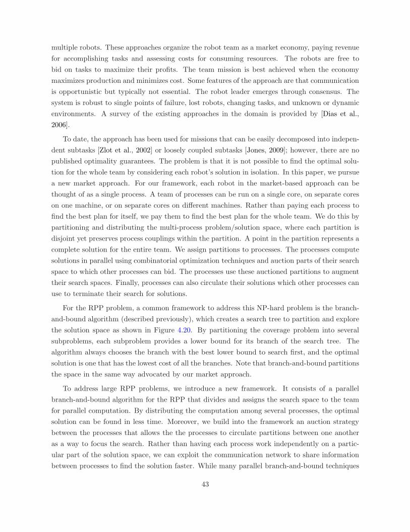
multiple robots. These approaches organize the robot team as a market economy, paying revenue

for accomplishing tasks and assessing costs for consuming resources. The robots are free to

bid on tasks to maximize their profits. The team mission is best achieved when the economy

maximizes production and minimizes cost. Some features of the approach are that communication

is opportunistic but typically not essential. The robot leader emerges through consensus. The

system is robust to single points of failure, lost robots, changing tasks, and unknown or dynamic

environments. A survey of the existing approaches in the domain is provided by [Dias et al.,

2006].

To date, the approach has been used for missions that can be easily decomposed into indepen-

dent subtasks [Zlot et al., 2002] or loosely coupled subtasks [Jones, 2009]; however, there are no

published optimality guarantees. The problem is that it is not possible to find the optimal solu-

tion for the whole team by considering each robot’s solution in isolation. In this paper, we pursue

a new market approach. For our framework, each robot in the market-based approach can be

thought of as a single process. A team of processes can be run on a single core, on separate cores

on one machine, or on separate cores on different machines. Rather than paying each process to

find the best plan for itself, we pay them to find the best plan for the whole team. We do this by

partitioning and distributing the multi-process problem/solution space, where each partition is

disjoint yet preserves process couplings within the partition. A point in the partition represents a

complete solution for the entire team. We assign partitions to processes. The processes compute

solutions in parallel using combinatorial optimization techniques and auction parts of their search

space to which other processes can bid. The processes use these auctioned partitions to augment

their search spaces. Finally, processes can also circulate their solutions which other processes can

use to terminate their search for solutions.

For the RPP problem, a common framework to address this NP-hard problem is the branch-

and-bound algorithm (described previously), which creates a search tree to partition and explore

the solution space as shown in Figure 4.20. By partitioning the coverage problem into several

subproblems, each subproblem provides a lower bound for its branch of the search tree. The

algorithm always chooses the branch with the best lower bound to search first, and the optimal

solution is one that has the lowest cost of all the branches. Note that branch-and-bound partitions

the space in the same way advocated by our market approach.

To address large RPP problems, we introduce a new framework. It consists of a parallel

branch-and-bound algorithm for the RPP that divides and assigns the search space to the team

for parallel computation. By distributing the computation among several processes, the optimal

solution can be found in less time. Moreover, we build into the framework an auction strategy

between the processes that allows the the processes to circulate partitions between one another

as a way to focus the search. Rather than having each process work independently on a partic-

ular part of the solution space, we can exploit the communication network to share information

between processes to find the solution faster. While many parallel branch-and-bound techniques

43

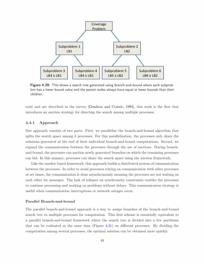
Figure 4.20: This shows a search tree generated using branch-and-bound where each subprob-lem has a lower bound value and the parent nodes always have equal or lower bounds than theirchildren.

exist and are described in the survey [Gendron and Crainic, 1994], this work is the first that

introduces an auction strategy for directing the search among multiple processes.

4.4.1 Approach

Our approach consists of two parts. First, we parallelize the branch-and-bound algorithm that

splits the search space among k processes. For this parallelization, the processes only share the

solutions generated at the end of their individual branch-and-bound computations. Second, we

expand the communication between the processes through the use of auctions. During branch-

and-bound, the processes can auction newly generated branches on which the remaining processes

can bid. In this manner, processes can share the search space using the auction framework.

Like the market-based framework, this approach builds a distributed system of communication

between the processes. In order to avoid processes relying on communication with other processes

at set times, the communication is done asynchronously meaning the processes are not waiting on

each other for messages. The lack of reliance on synchroneity constraints enables the processes

to continue processing and working on problems without delays. This communication strategy is

useful when communication interruptions or network outages occur.

Parallel Branch-and-bound

The parallel branch-and-bound approach is a way to assign branches of the branch-and-bound

search tree to multiple processes for computation. This first scheme is essentially equivalent to

a parallel branch-and-bound framework where the search tree is divided into a few partitions

that can be evaluated at the same time (Figure 4.21) on different processes. By dividing the

computation among several processes, the optimal solution can be obtained more quickly.

44

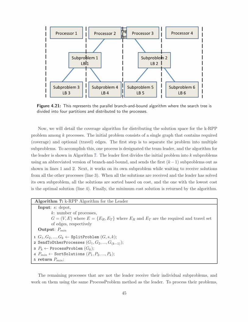
Figure 4.21: This represents the parallel branch-and-bound algorithm where the search tree isdivided into four partitions and distributed to the processes.

Now, we will detail the coverage algorithm for distributing the solution space for the k-RPP

problem among k processes. The initial problem consists of a single graph that contains required

(coverage) and optional (travel) edges. The first step is to separate the problem into multiple

subproblems. To accomplish this, one process is designated the team leader, and the algorithm for

the leader is shown in Algorithm 7. The leader first divides the initial problem into k subproblems

using an abbreviated version of branch-and-bound, and sends the first (k−1) subproblems out as

shown in lines 1 and 2. Next, it works on its own subproblem while waiting to receive solutions

from all the other processes (line 3). When all the solutions are received and the leader has solved

its own subproblem, all the solutions are sorted based on cost, and the one with the lowest cost

is the optimal solution (line 4). Finally, the minimum cost solution is returned by the algorithm.

Algorithm 7: k-RPP Algorithm for the Leader

Input: s: depot,k: number of processes,G = (V,E) where E = {ER, ET } where ER and ET are the required and travel setof edges, respectively

Output: Pmin

1 G1, G2, ..., Gk ← SplitProblem (G, s, k);2 SendToOtherProcesses (G1, G2, ..., G(k−1));

3 Pk ← ProcessProblem (Gk);4 Pmin ← SortSolutions (P1, P2, ..., Pk);5 return Pmin;

The remaining processes that are not the leader receive their individual subproblems, and

work on them using the same ProcessProblem method as the leader. To process their problems,

45

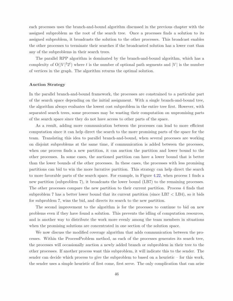
each processes uses the branch-and-bound algorithm discussed in the previous chapter with the

assigned subproblem as the root of the search tree. Once a processes finds a solution to its

assigned subproblem, it broadcasts the solution to the other processes. This broadcast enables

the other processes to terminate their searches if the broadcasted solution has a lower cost than

any of the subproblems in their search trees.

The parallel RPP algorithm is dominated by the branch-and-bound algorithm, which has a

complexity of O(|V |32t) where t is the number of optional path segments and |V | is the number

of vertices in the graph. The algorithm returns the optimal solution.

Auction Strategy

In the parallel branch-and-bound framework, the processes are constrained to a particular part

of the search space depending on the initial assignment. With a single branch-and-bound tree,

the algorithm always evaluates the lowest cost subproblem in the entire tree first. However, with

separated search trees, some processes may be wasting their computation on unpromising parts

of the search space since they do not have access to other parts of the space.

As a result, adding more communication between the processes can lead to more efficient

computation since it can help direct the search to the more promising parts of the space for the

team. Translating this idea to parallel branch-and-bound, when several processes are working

on disjoint subproblems at the same time, if communication is added between the processes,

when one process finds a new partition, it can auction the partition and lower bound to the

other processes. In some cases, the auctioned partition can have a lower bound that is better

than the lower bounds of the other processes. In these cases, the processes with less promising

partitions can bid to win the more lucrative partition. This strategy can help direct the search

to more favorable parts of the search space. For example, in Figure 4.22, when process 1 finds a

new partition (subproblem 7), it broadcasts the lower bound (LB7) to the remaining processes.

The other processes compare the new partition to their current partition. Process 4 finds that

subproblem 7 has a better lower bound that its current partition (since LB7 < LB4), so it bids

for subproblem 7, wins the bid, and directs its search to the new partition.

The second improvement to the algorithm is for the processes to continue to bid on new

problems even if they have found a solution. This prevents the idling of computation resources,

and is another way to distribute the work more evenly among the team members in situations

when the promising solutions are concentrated in one section of the solution space.

We now discuss the modified coverage algorithm that adds communication between the pro-

cesses. Within the ProcessProblem method, as each of the processes generates its search tree,

the processes will occasionally auction a newly added branch or subproblem in their tree to the

other processes. If another process want this subproblem, it will indicate this to the sender. The

sender can decide which process to give the subproblem to based on a heuristic – for this work,

the sender uses a simple heuristic of first come, first serve. The only complication that can arise

46

Figure 4.22: Communication strategy where each process is working on a part of the searchtree. With communication, process 1 is able to auction part of its search, subproblem 7, toother processes. In this case, process 4 decides to accept subproblem 7 from process 1.

is if the sender itself is currently processing the subproblem (this can occur if the subproblem

had a low cost and low cost subproblems are processed first). In this situation, the sender does

not send the subproblem out.

4.4.2 Testing Framework

Our tests evaluated the performance of the parallel branch-and-bound algorithm and the auction

strategy. We ran the tests on a single machine with four processing units, each of which contained

a 2.67GHz Intel Core i5 processor; they all shared 8GB of RAM. Each process ran on a separate

core. One process was designated the leader. Each process communicated with the others through

the network layer using the TCP protocol.

To enable communication, each process consisted of two threads. One thread was dedicated to

the branch-and-bound search processing, and the other focused on the networking. Each process

started a server with a specific address and a client, both of which communicated across the

socket layer.

There were two main sets of tests: one evaluating the performance of the parallel branch-and-

bound algorithm without the auction strategy, and the second evaluating the parallel branch-

and-bound with the auction strategy. To describe the testing framework, we will first explain

the test graphs, then the procedure for each test, and finally present the metrics for performance

evaluation.

For our testing, we used rectilinear graphs. Three graph sizes were used: {10×10, 14×14, 17×

17}. For each graph, a random set of edges were selected to be travel. To keep computation time

reasonable, graphs that took longer than 10 minutes to find a solution were excluded from the

test set.

47

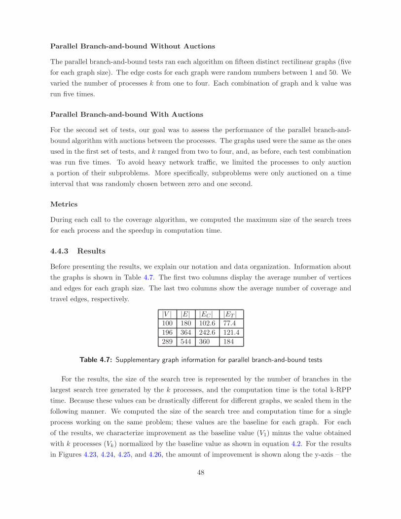
Parallel Branch-and-bound Without Auctions

The parallel branch-and-bound tests ran each algorithm on fifteen distinct rectilinear graphs (five

for each graph size). The edge costs for each graph were random numbers between 1 and 50. We

varied the number of processes k from one to four. Each combination of graph and k value was

run five times.

Parallel Branch-and-bound With Auctions

For the second set of tests, our goal was to assess the performance of the parallel branch-and-

bound algorithm with auctions between the processes. The graphs used were the same as the ones

used in the first set of tests, and k ranged from two to four, and, as before, each test combination

was run five times. To avoid heavy network traffic, we limited the processes to only auction

a portion of their subproblems. More specifically, subproblems were only auctioned on a time

interval that was randomly chosen between zero and one second.

Metrics

During each call to the coverage algorithm, we computed the maximum size of the search trees

for each process and the speedup in computation time.

4.4.3 Results

Before presenting the results, we explain our notation and data organization. Information about

the graphs is shown in Table 4.7. The first two columns display the average number of vertices

and edges for each graph size. The last two columns show the average number of coverage and

travel edges, respectively.

|V | |E| |EC | |ET |

100 180 102.6 77.4

196 364 242.6 121.4

289 544 360 184

Table 4.7: Supplementary graph information for parallel branch-and-bound tests

For the results, the size of the search tree is represented by the number of branches in the

largest search tree generated by the k processes, and the computation time is the total k-RPP

time. Because these values can be drastically different for different graphs, we scaled them in the

following manner. We computed the size of the search tree and computation time for a single

process working on the same problem; these values are the baseline for each graph. For each

of the results, we characterize improvement as the baseline value (V1) minus the value obtained

with k processes (Vk) normalized by the baseline value as shown in equation 4.2. For the results

in Figures 4.23, 4.24, 4.25, and 4.26, the amount of improvement is shown along the y-axis – the

48

Figure 4.23: Improvement in the number of branches in the search tree for the coveragealgorithm with no auctions. The number of processors ranged from two to four.

higher the value, the better the performance. Additionally, in these figures, the x-axis denotes

the set of fifteen test graphs and the y-axis values are the averages over the five trials for each

graph.

Improvementk =V1 − Vk

V1(4.2)

Parallel Branch-and-bound Without Auctions

The results show that dividing the work between multiple processes helps reduce the size of the

maximum search tree by decreasing the number of branches in the tree (Fig. 4.23). Since the

solution space is initially split into k sections and the optimal solution resides in one of these

sections, in most cases, the work is not distributed evenly among the processes. However, based

on the results, it is clear that increasing the number of processes can reduce the size of the

maximum individual search trees such as for graphs 6 and 9. In terms of total computation time,

for most of the graphs, using more processors leads to a decrease in runtime. However, there

is an overhead in the parallel k-RPP algorithm with two or more processes since it consists of

splitting the initial problem, and includes some time costs due to communication. For graph 3 in

Fig. 4.24, the computation time gets worse when more than one process is used to parallelize the

search effort. For this particular graph, because the runtime of search using a single process is

fairly low at 1.5 seconds, the overhead costs are relatively high in comparison. As a result, there

is an increase in computation time leading to a decline in performance with more processes. Since

most of the coverage problems that are solved using branch-and-bound are computationally more

expensive, the overhead of adding communication is negligible as shown by the remaining graph

instances.

49

Figure 4.24: Improvement in the total computation time for the coverage algorithm with noauctions. The number of processors ranged from two to four.

Figure 4.25: Improvement in the number of branches in the search tree for the coveragealgorithm with auctions. The number of processors ranged from two to four.

50

Figure 4.26: Improvement in the computation time for the coverage algorithm with auctions.The number of processors ranged from two to four.

Parallel Branch-and-bound With Auctions

Adding the auction strategy to the parallel k-RPP algorithm enables the processes to share the

work better by distributing problems more evenly. Overall, the addition of the auctions improves

the efficiency of the search algorithm by reducing the number of branches as shown in Figure 4.25.

Compared with the same algorithm run without auctions, the performance for all instances of k

improves when information is shared. In some instances, such as graph 1, the relative differences

between the improvements for the different values of k shrinks. Furthermore, in many cases,

the use of auctions enables a team of processes to perform much better than a larger team size.

For example, for graph 12, two processors using the auction strategy performs roughly twice

as well as four processors without auctions. There is less improvement with graph 3 because

the search tree is small, meaning there is not a lot of room for improvement in general. With

more communication between the processes, there is a higher overhead which is reflected in the

computation times in Figure 4.26. These overhead costs can mask the improvement which occurs

with graphs 3 and 8.

We consider the single process as the baseline in terms of search tree size. In the ideal case,

having four processes would divide the work evenly between them. However, this would require

close to perfect sharing of work so that no process will do any extra work. In the ideal case, if the

total work is represented as 1, then the amount of work each process does is 1kand the amount

of improvement each process would achieve in the parallel branch-and-bound framework is1− 1

k

1 .

When k ranges from 2 to 4, this ideal improvement would be 0.5, 0.66, and 0.75, respectively.

Looking at Figure 4.25, for tests 9 through 15, the use of auctions with parallel branch-and-bound

enables each process to generate a search tree that is extremely close in size to that of a single

process. This shows that auctions truly do allow multiple processes to act as one cohesive unit

51

when sharing the computation work in solving a problem.

4.4.4 Discussion

Our results indicate that parallelizing the branch-and-bound algorithm, and employing auctions

between the processes can solve large coverage problems more efficiently. Distributing the search

tree among k processes alone may not result in major improvements in efficiency since the promis-

ing solutions may not be distributed evenly among the partitions. In some cases, the size of the

search tree with more processes is the same as for a single process, as shown by graphs 4, 10, and

11 in Figure 4.23. However, for problems such as those shown in graphs 6 and 9, distributing the

initial problem can significantly reduce the branching factor in the search process.

When auctions occur between the processes, efficiency substantially increases for all values

of k. The auctioning of subproblems during the search process allows the processes to share the

whole search space. In this manner, the k processes act more like a single process since they

have access to and can evaluate solutions outside their initial assignment. In most instances,

auctioning subproblems helps reduce the amount of computation performed by each process.

However, in some instances, the sharing of subproblems can lead to certain branches which may

look promising but are dead ends to be distributed among all the processes. In this case, this

could lead to a larger search tree and high computation time such as the case of graph 5 with

four processes in Figures 4.25 and 4.26.

For this implementation, we adhere to a relatively simple auction framework and bidding

strategy. It would be interesting to analyze more complicated auction strategies where only

certain subproblems are offered to the other processes. Rather than auctioning the problems at

certain time intervals, strategies such as auctioning problems when the priority queue is more than

a certain size limit or auctioning only problems that have high lower bounds are ways to only share

work when necessary. Likewise, bidding strategies can also make better use of other information.

For example, a process’s bid on an auctioned problem could be the difference between its own

lowest cost problem and the problem being auctioned. In this way, the auctioneer can choose

the bid with the highest value in an effort to ensure the team always works on the lowest cost

problem at any point in time.

4.5 Conclusion

This chapter addresses the problem of partial environmental coverage with a single robot. When

representing the environment as a graph, the problem translates to a Rural Postman problem. An

optimal algorithm for this problem is introduced that uses the idea of path segments instead of

edges as the partition set for building the branch-and-bound search tree. While the algorithm can

find a solution for any graph, it is more computationally efficient on graphs where the number

of travel edges is relatively low, and the coverage components are sparse. To aid replanning

52

when graph updates occur, a heuristic is introduced into the path building method that seeks

to maintain connectivity of the coverage edges in the path. This strategy aims to prevent the

problem from becoming more complex when a replan is required. Both the use of path segments

in the branch-and-bound algorithm and the path building heuristic are shown to improve the

runtime of finding an optimal solution during replanning.

For many RPP problems, the branch-and-bound problem can be large, making it computa-

tionally expensive to solve the problem. To handle large problems, we introduce a framework

that parallelizes the branch-and-bound computation among several processes. Similar to market-

based systems for multi-robot coordination, the parallel branch-and-bound approach includes an

auction framework whereby a process can offer parts of its work to other members of the team.

For these problems, this auction system allow the processes to share the search tree in a way that

enables them to act like a single unit and find the solution faster. As the results show, in some

cases, the computation can be distributed so well that no process incurs extra work when using

the parallel branch-and-bound approach.

53

54

Chapter 5

Partial Coverage with Multiple

Robots without Environmental

Constraints

In this chapter, we extend the partial coverage problem from a single robot to multiple robots. To

maintain a computationally efficient runtime, the approaches that we introduce are approximate

rather than optimal.

For this area of work, we seek k coverage paths that visit a designated subset of the graph

edges where k is the number of robots. This coverage problem can be modeled as an arc-routing

problem. We focus on two types of arc-routing problems: the k-Chinese Postman Problem and

the k-Rural Postman Problem. The k-Chinese Postman Problem (k -CPP) seeks k paths that

visit all the edges of the graph at least once. The k-Rural Postman Problem (k-RPP) seeks k

paths that visit a predefined subset of graph edges at least once.

The objectives of a multiple robot routing problem can vary. Common objectives include

minimizing resource usage, time, or cost of the total plan. We focus on minimizing the path cost

of the worst performing robot. This goal is appropriate for the problems that we are addressing

because we have allocated a team of robots for a particular task, and want the work to be divided

evenly among the members of the team. This means no single robot should be performing more

work than the others. If minimizing the resource usage or total path cost were the objective,

in some cases the optimal plan would be to only use one robot to perform a task and the total

mission time would be much higher. Existing work in the area of multiple robots have cautioned

against the objective of minimizing total path cost if reducing traversal time is important, which

is usually the case for most practical applications [Mosteo and Montano, 2007]. Moreover, having

multiple robots adds a degree of redundancy to the solution. If one robot was used and it broke

down, another robot would have to start from the depot or starting position to complete the task.

If multiple robots were used, another robot would already be traversing the environment and be

55

available to finish the task.

When multiple robots are added to the coverage problem, we focus on approximation algo-

rithms since an optimal solution cannot be efficiently obtained. As a result, we choose to tackle

this problem using a “divide and conquer” technique, but consider the two steps as interchange-

able. Hence, we use two common approaches that have been introduced for arc routing problems

with multiple agents: a Cluster First, Route Second (C1R2) paradigm and a Route First, Cluster

Second (R1C2) paradigm.

The C1R2 approach first separates the space into separate sections, one for each robot. It

then computes a solution for each cluster using the lower-complexity single robot algorithm. On

the other hand, the R1C2 approach first poses the problem as a single robot lower-complexity

coverage problem; once a solution is found for a single robot, the solution is then separated into

one path for each robot. Although we are not producing an exact solution, the division of the

problem into two separate subproblems does allow the use of lower complexity approximations,

some of which have guarantees with regard to the optimal solution. We discuss each approach in

the next few sections.

5.1 Cluster First, Route Second Approach

To our knowledge, only one algorithm exists for the k-RPP. The algorithm is a C1R2 heuristic

algorithm [Easton and Burdick, 2005]. The k-RPP algorithm consists of four steps: first, it

divides the graph into k clusters using a method [Ahr, 2004] based on the farthest-point clustering

algorithm [Gonzalez, 1985]. Second, it connects the edges in each cluster by creating a spanning

tree between the disconnected components. Third, it utilizes the CPP algorithm to find a route

for each cluster. Finally, the algorithm refines each cluster by removing extraneous edges at the

end of the tour once all the required edges have been visited. The extra edges are replaced by

the shortest path to the depot from the final required edge in the tour. While the k robots are

assumed to start from the same depot for the static algorithm, the dynamic version [Williams

and Burdick, 2006] handles varying starting locations and changes within the graph and team

size.

In this section, we present a k-RPP algorithm with two major improvements over the prior

algorithm detailed above. The first improvement is to the clustering step. It enables a better

division of the graph edges into k partitions. The second improvement is to the routing step.

It allows for shorter tours of the clusters by using the optional edges to connect required edges.

These two improvements to the algorithm help generate more evenly-distributed paths for faster

coverage of the environment.

56

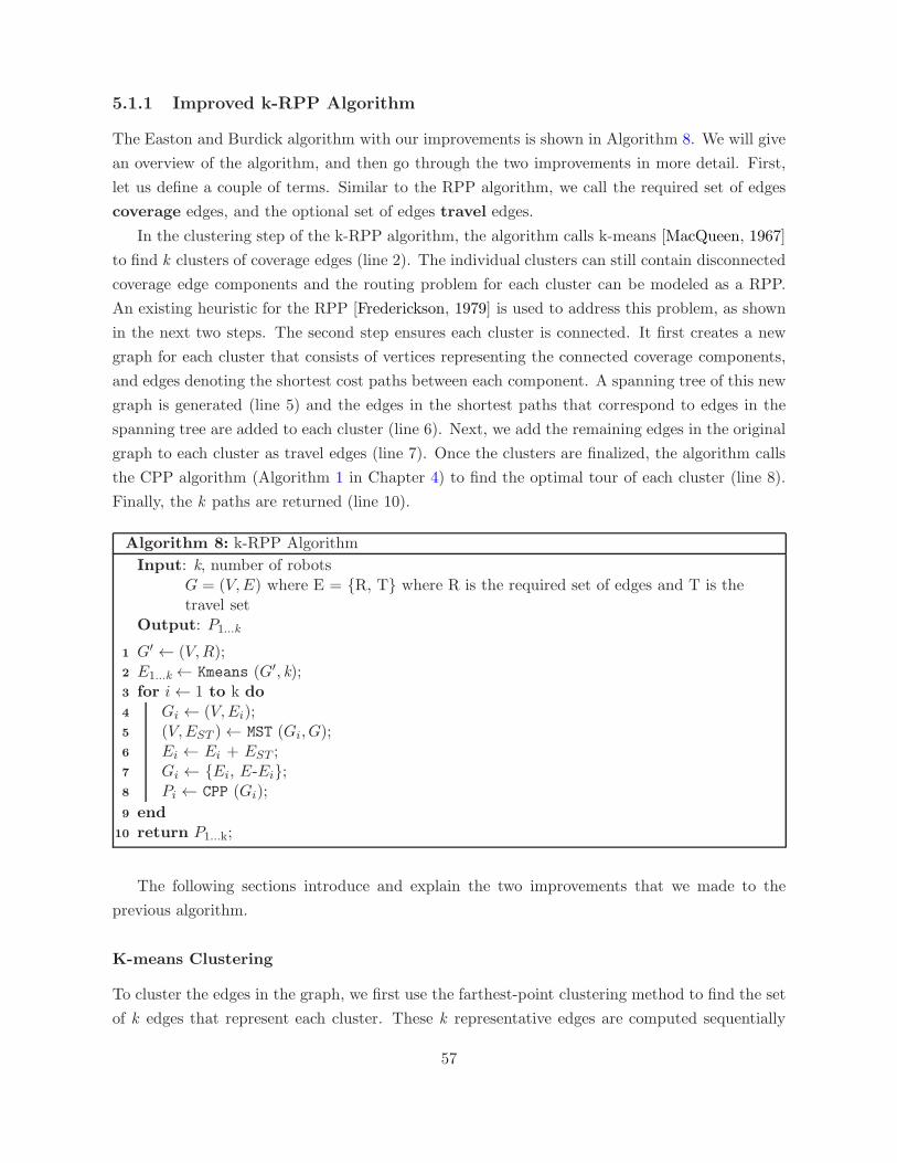
5.1.1 Improved k-RPP Algorithm

The Easton and Burdick algorithm with our improvements is shown in Algorithm 8. We will give

an overview of the algorithm, and then go through the two improvements in more detail. First,

let us define a couple of terms. Similar to the RPP algorithm, we call the required set of edges

coverage edges, and the optional set of edges travel edges.

In the clustering step of the k-RPP algorithm, the algorithm calls k-means [MacQueen, 1967]

to find k clusters of coverage edges (line 2). The individual clusters can still contain disconnected

coverage edge components and the routing problem for each cluster can be modeled as a RPP.

An existing heuristic for the RPP [Frederickson, 1979] is used to address this problem, as shown

in the next two steps. The second step ensures each cluster is connected. It first creates a new

graph for each cluster that consists of vertices representing the connected coverage components,

and edges denoting the shortest cost paths between each component. A spanning tree of this new

graph is generated (line 5) and the edges in the shortest paths that correspond to edges in the

spanning tree are added to each cluster (line 6). Next, we add the remaining edges in the original

graph to each cluster as travel edges (line 7). Once the clusters are finalized, the algorithm calls

the CPP algorithm (Algorithm 1 in Chapter 4) to find the optimal tour of each cluster (line 8).

Finally, the k paths are returned (line 10).

Algorithm 8: k-RPP Algorithm

Input: k, number of robotsG = (V,E) where E = {R, T} where R is the required set of edges and T is thetravel set

Output: P1...k

1 G′ ← (V,R);2 E1...k ← Kmeans (G′, k);3 for i← 1 to k do4 Gi ← (V,Ei);5 (V,EST )← MST (Gi, G);6 Ei ← Ei + EST ;7 Gi ← {Ei, E-Ei};8 Pi ← CPP (Gi);

9 end10 return P1...k;

The following sections introduce and explain the two improvements that we made to the

previous algorithm.

K-means Clustering

To cluster the edges in the graph, we first use the farthest-point clustering method to find the set

of k edges that represent each cluster. These k representative edges are computed sequentially

57

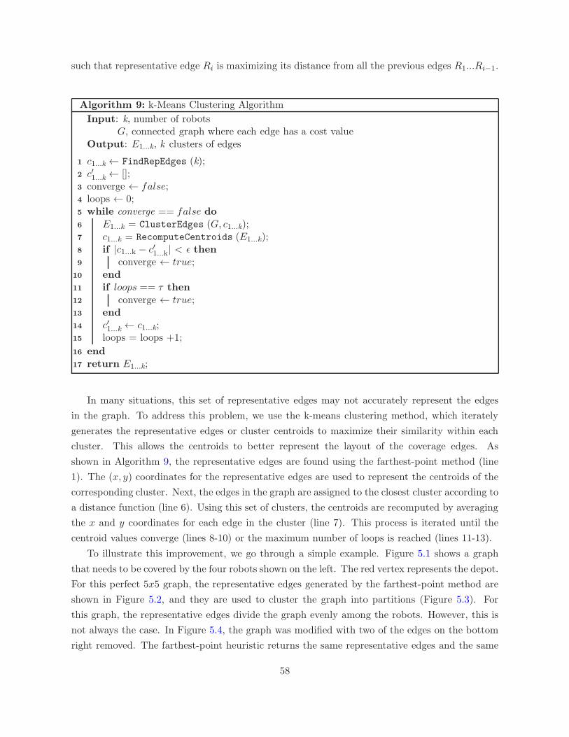
such that representative edge Ri is maximizing its distance from all the previous edges R1...Ri−1.

Algorithm 9: k-Means Clustering Algorithm

Input: k, number of robotsG, connected graph where each edge has a cost value

Output: E1...k, k clusters of edges

1 c1...k ← FindRepEdges (k);2 c′1...k ← [];3 converge ← false;4 loops ← 0;5 while converge == false do6 E1...k = ClusterEdges (G, c1...k);7 c1...k = RecomputeCentroids (E1...k);8 if |c1...k − c′1...k| < ǫ then9 converge ← true;

10 end11 if loops == τ then12 converge ← true;13 end14 c′1...k ← c1...k;15 loops = loops +1;

16 end17 return E1...k;

In many situations, this set of representative edges may not accurately represent the edges

in the graph. To address this problem, we use the k-means clustering method, which iterately

generates the representative edges or cluster centroids to maximize their similarity within each

cluster. This allows the centroids to better represent the layout of the coverage edges. As

shown in Algorithm 9, the representative edges are found using the farthest-point method (line

1). The (x, y) coordinates for the representative edges are used to represent the centroids of the

corresponding cluster. Next, the edges in the graph are assigned to the closest cluster according to

a distance function (line 6). Using this set of clusters, the centroids are recomputed by averaging

the x and y coordinates for each edge in the cluster (line 7). This process is iterated until the

centroid values converge (lines 8-10) or the maximum number of loops is reached (lines 11-13).

To illustrate this improvement, we go through a simple example. Figure 5.1 shows a graph

that needs to be covered by the four robots shown on the left. The red vertex represents the depot.

For this perfect 5x5 graph, the representative edges generated by the farthest-point method are

shown in Figure 5.2, and they are used to cluster the graph into partitions (Figure 5.3). For

this graph, the representative edges divide the graph evenly among the robots. However, this is

not always the case. In Figure 5.4, the graph was modified with two of the edges on the bottom

right removed. The farthest-point heuristic returns the same representative edges and the same

58

Figure 5.1: An example of the clustering al-gorithms on this 5x5 graph with four robots.The depot vertex is red while the remainingvertices are blue. The vertices are connectedby edges denoted by the blue lines.

Figure 5.2: The farthest-point clusteringmethod finds four representative edges in thegraph which are denoted by the orange lines.

Figure 5.3: The edges in the graph are thenclustered into four partitions using the rep-resentative edges.

Figure 5.4: Next, we test the farthest-pointmethod on a slightly modified 5x5 graphwhere two of the edges are removed (rightbottom). k is still four in this case.

59

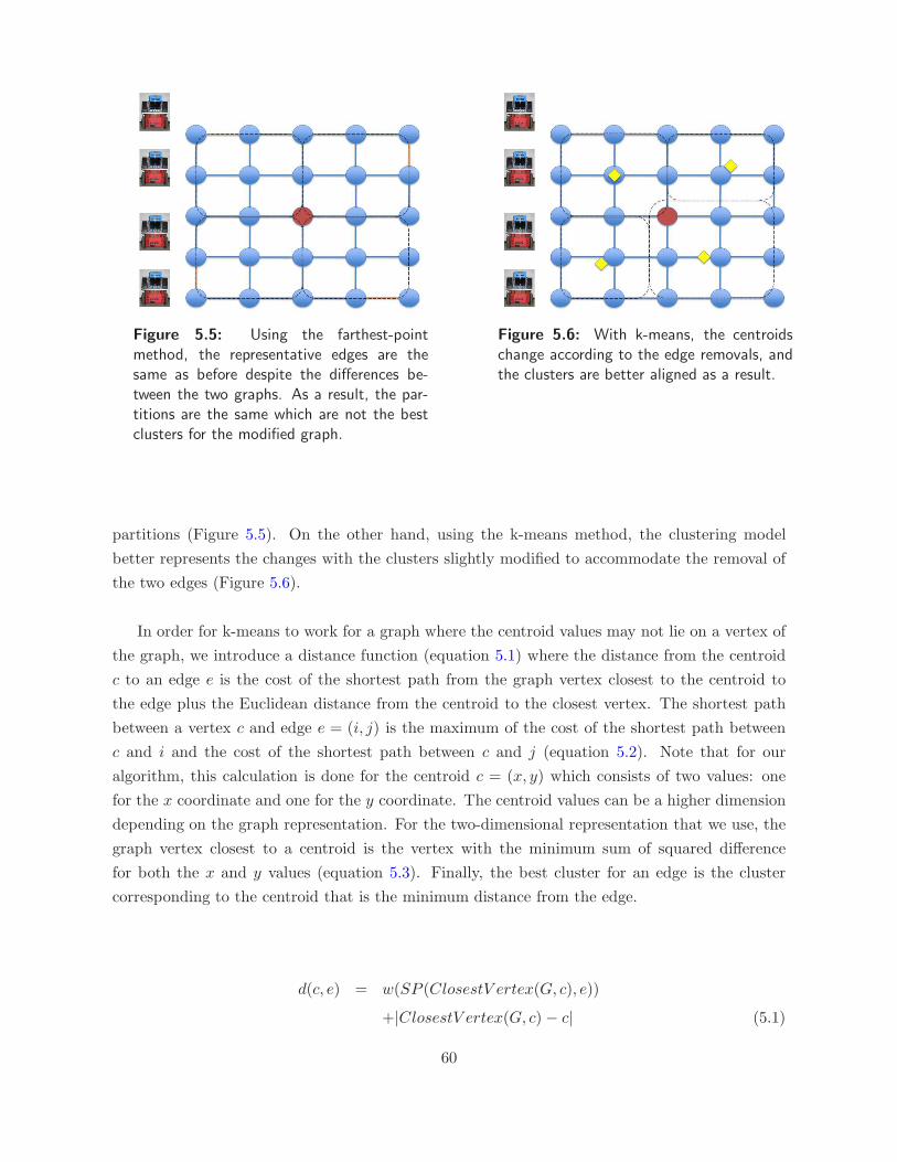
Figure 5.5: Using the farthest-pointmethod, the representative edges are thesame as before despite the differences be-tween the two graphs. As a result, the par-titions are the same which are not the bestclusters for the modified graph.

Figure 5.6: With k-means, the centroidschange according to the edge removals, andthe clusters are better aligned as a result.

partitions (Figure 5.5). On the other hand, using the k-means method, the clustering model

better represents the changes with the clusters slightly modified to accommodate the removal of

the two edges (Figure 5.6).

In order for k-means to work for a graph where the centroid values may not lie on a vertex of

the graph, we introduce a distance function (equation 5.1) where the distance from the centroid

c to an edge e is the cost of the shortest path from the graph vertex closest to the centroid to

the edge plus the Euclidean distance from the centroid to the closest vertex. The shortest path

between a vertex c and edge e = (i, j) is the maximum of the cost of the shortest path between

c and i and the cost of the shortest path between c and j (equation 5.2). Note that for our

algorithm, this calculation is done for the centroid c = (x, y) which consists of two values: one

for the x coordinate and one for the y coordinate. The centroid values can be a higher dimension

depending on the graph representation. For the two-dimensional representation that we use, the

graph vertex closest to a centroid is the vertex with the minimum sum of squared difference

for both the x and y values (equation 5.3). Finally, the best cluster for an edge is the cluster

corresponding to the centroid that is the minimum distance from the edge.

d(c, e) = w(SP (ClosestV ertex(G, c), e))

+|ClosestV ertex(G, c) − c| (5.1)

60

SP (ClosestV ertex(G, c), e = (i, j)) = max(w(SP (ClosestV ertex(G, c), i),

w(SP (ClosestV ertex(G, c), j)) (5.2)

ClosestV ertex(G, c = (cx, cy)) = argminv=(vx,vy)(vx − cx)2 + (vy − cy)

2 (5.3)

Use of Travel Edges

In the prior k-RPP algorithm [Easton and Burdick, 2005], after clustering all the edges, the

CPP algorithm generates a path for each cluster, and the path is refined. We implemented an

improvement to these two steps that enables the removal of the refinement step by having the

CPP find the optimal plan for each cluster of coverage edges. In order to generate an Eulerian

tour, the CPP algorithm must decide which edges in the graph to traverse twice; these edges

would be doubled in the solution. To maintain a low cost path, it is important to double the

minimum cost set of edges. Therefore, if we allow travel edges as well as coverage edges to be

doubled, the doubled set may have a lower cost than if we only consider coverage edges.

5.1.2 Dynamic k-RPP Algorithm

Dynamic changes occur when the environment differs from the original map. For the coverage

problems we are addressing in this work, most changes to the environment are discovered when

the robots are actively traversing the space. These online changes are typically detected when the

robots have traveled to middle locations along the coverage path and have already visited some

of the edges. Because it is not necessary to revisit those edges, the visited edges in the previous

plans are converted to travel edges.

To replan with the robots starting at a different location from the depot or goal location, we

extend an idea that we used with the single robot RPP. To account for different start and end

locations, we add an artificial edge to each of the k clusters that has one endpoint at the current

robot location and the other endpoint at the depot. This edge is assigned a large cost to ensure

it is not doubled in the solution. After the k tours are found, the artificial edge in each tour is

removed and the paths are adjusted to start at the current robot positions.

To illustrates the online coverage algorithm, in Figure 5.7, we show a k-CPP solution of

the example graph shown previously. In Figure 5.8, four robots (blue, red, cyan, and magenta)

traverse the initial paths until one of them (blue) discovers that an edge in its path is missing. The

robot does not know about this discrepancy until it reaches the adjacent vertex. The algorithm

then sets the traversed edges in the four paths to be travel edges (Figure 5.9) and the problem

becomes a k-RPP. The replanned coverage tours are shown in Figure 5.10.

61

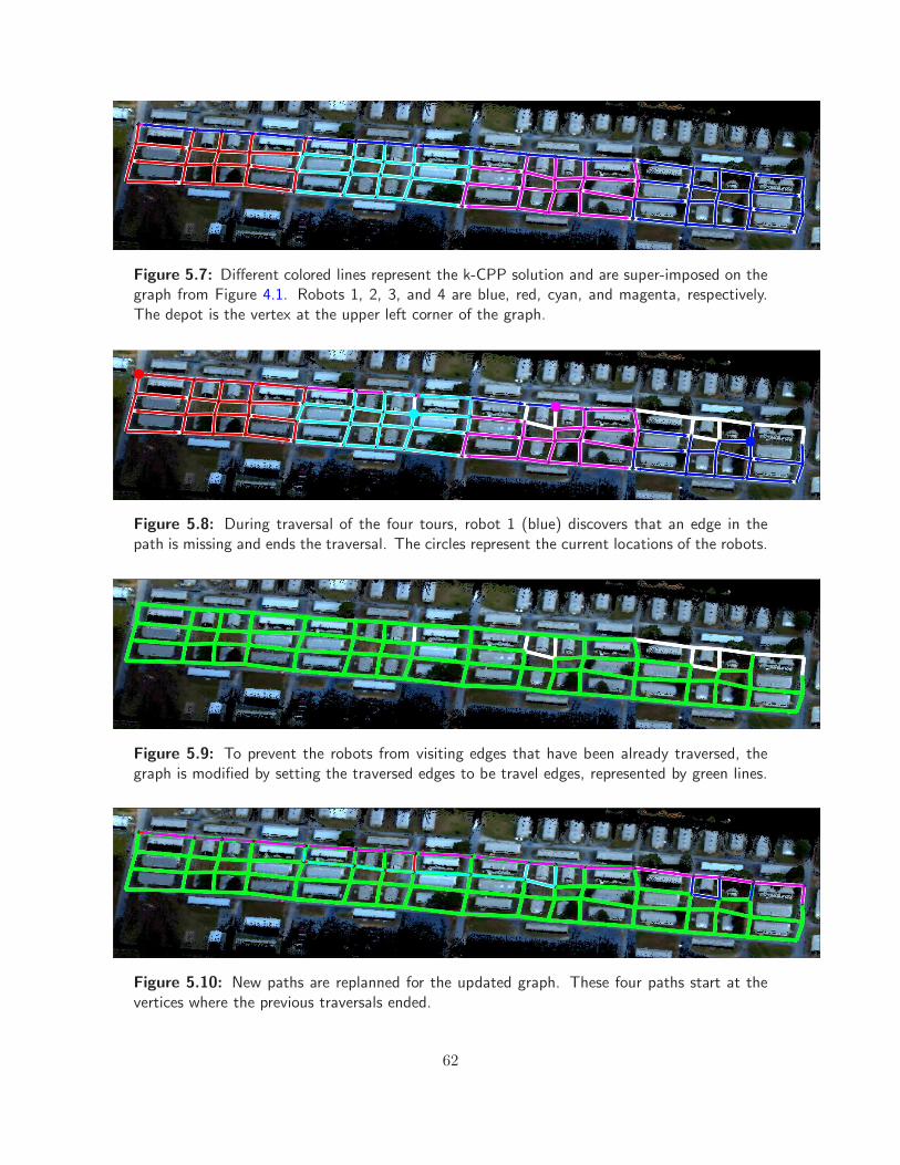
Figure 5.7: Different colored lines represent the k-CPP solution and are super-imposed on thegraph from Figure 4.1. Robots 1, 2, 3, and 4 are blue, red, cyan, and magenta, respectively.The depot is the vertex at the upper left corner of the graph.

Figure 5.8: During traversal of the four tours, robot 1 (blue) discovers that an edge in thepath is missing and ends the traversal. The circles represent the current locations of the robots.

Figure 5.9: To prevent the robots from visiting edges that have been already traversed, thegraph is modified by setting the traversed edges to be travel edges, represented by green lines.

Figure 5.10: New paths are replanned for the updated graph. These four paths start at thevertices where the previous traversals ended.

62

One advantage to this revision strategy is that it supports the case where the robots start at

different depots. Instead of all robots starting at the same depot, different robots can start at

different depots. Morever, this method can be easily extended to handle changing team sizes (for

example, due to robot failure or new robots entering the scene) by excluding the artificial edge

corresponding to the failed robot or not having artificial edges for the new robots, respectively.

We considered using the the revision algorithm given in [Williams and Burdick, 2006] which,

when replanning, uses the next edge in the original path of each robot as the representative edge

for its new cluster. While this method works well on graphs where the clusters are far apart,

it does not perform as well when the clusters are close together, particularly in situations when

some of the robots are at the same location. In this case, the representative edges of the clusters

corresponding to those robots would be the same, and the resulting clusters would not be well

distributed.

5.1.3 Comparison Tests

Our testing compared the improved k-RPP algorithm against the original k-RPP algorithm. For

the tests, we wanted to assess the two algorithmic improvements, k-means clustering and travel

edges usage, individually. To do this, we compared four combinations of the algorithm: the

original algorithm, the original algorithm with k-means clustering, the original algorithm using

travel edges, and the original algorithm with both improvements (our algorithm). For the tests,

we varied four different parameters: algorithm combination, size of graph, starting vertex s, and

number of robots k. The test simulated k robots executing k tours starting at vertex s.

We conducted two sets of tests: static and dynamic k-RPP tests. The first test set evaluated

the algorithm combinations on four graphs. The second test set demonstrated the replanning

capability of the algorithm when handling online changes. We will first explain the procedure

for each test, and then present the metrics for comparing the two heuristics. The code ran on a

machine with a 2.53GHz Intel processor and 4GB of RAM.

Static k-RPP Tests

The first set of tests ran each algorithm on four different graphs: three rectilinear graphs and

one real-world road network dataset. We ran five trials on each graph with each trial having a

random set of travel edges. Each set of travel edges constituted half of the edges in the graph.

The results were averaged over the five trials. The number of robots, k, ranged from one to ten.

For the rectilinear graphs and each k value, we varied the starting vertex over all the vertices in

the graph to avoid bias. Therefore, each of the algorithm combinations was called k× 3× 5× |V |

times where |V | is the number of vertices in the graph. Because the road network graph is so

large, instead of varying the starting vertex over all vertices in the graph, we sampled a set of fifty

distinct vertices. The samples were consistent for the four methods. In total, the road network

test yielded k× 5× 50 plans for each combination.

63

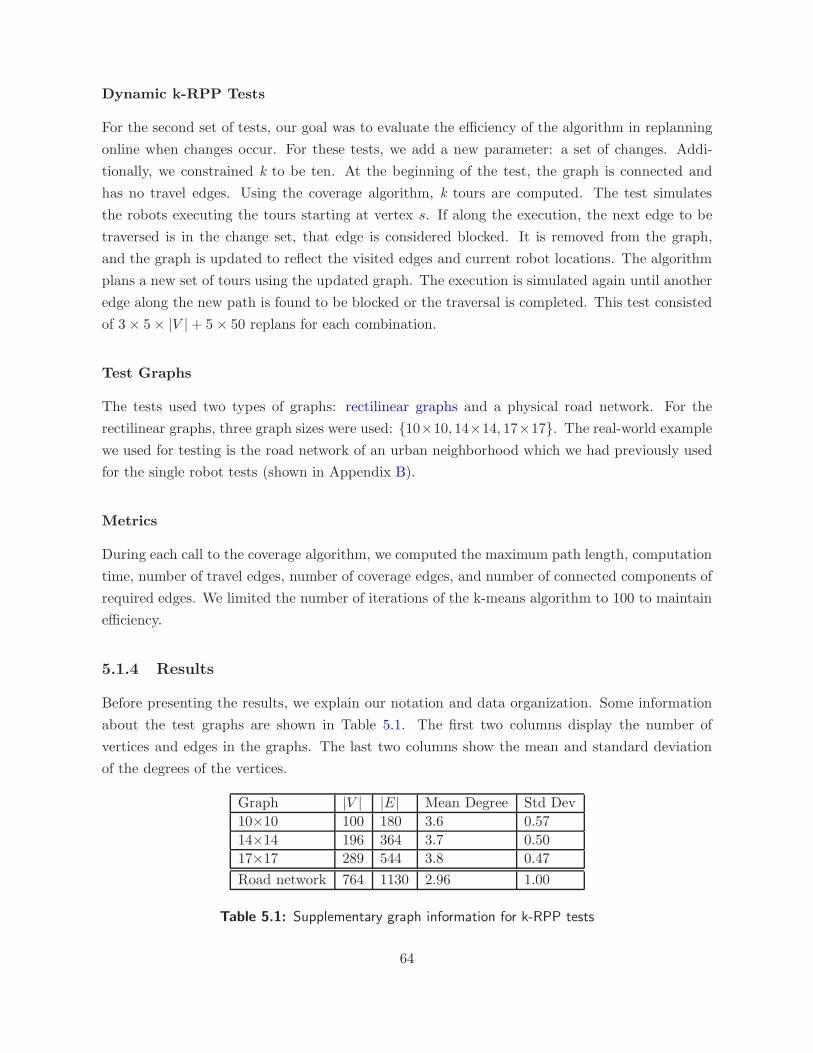
Dynamic k-RPP Tests

For the second set of tests, our goal was to evaluate the efficiency of the algorithm in replanning

online when changes occur. For these tests, we add a new parameter: a set of changes. Addi-

tionally, we constrained k to be ten. At the beginning of the test, the graph is connected and

has no travel edges. Using the coverage algorithm, k tours are computed. The test simulates

the robots executing the tours starting at vertex s. If along the execution, the next edge to be

traversed is in the change set, that edge is considered blocked. It is removed from the graph,

and the graph is updated to reflect the visited edges and current robot locations. The algorithm

plans a new set of tours using the updated graph. The execution is simulated again until another

edge along the new path is found to be blocked or the traversal is completed. This test consisted

of 3× 5× |V |+ 5× 50 replans for each combination.

Test Graphs

The tests used two types of graphs: rectilinear graphs and a physical road network. For the

rectilinear graphs, three graph sizes were used: {10×10, 14×14, 17×17}. The real-world example

we used for testing is the road network of an urban neighborhood which we had previously used

for the single robot tests (shown in Appendix B).

Metrics

During each call to the coverage algorithm, we computed the maximum path length, computation

time, number of travel edges, number of coverage edges, and number of connected components of

required edges. We limited the number of iterations of the k-means algorithm to 100 to maintain

efficiency.

5.1.4 Results

Before presenting the results, we explain our notation and data organization. Some information

about the test graphs are shown in Table 5.1. The first two columns display the number of

vertices and edges in the graphs. The last two columns show the mean and standard deviation

of the degrees of the vertices.

Graph |V | |E| Mean Degree Std Dev

10×10 100 180 3.6 0.57

14×14 196 364 3.7 0.50

17×17 289 544 3.8 0.47

Road network 764 1130 2.96 1.00

Table 5.1: Supplementary graph information for k-RPP tests

64

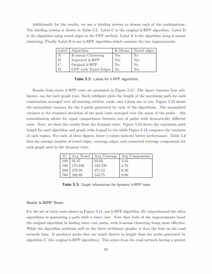
Additionally for the results, we use a labeling system to denote each of the combinations.

The labeling system is shown in Table 5.2. Label C is the original k-RPP algorithm. Label D

is the algorithm using travel edges in the CPP method. Label A is the algorithm using k-means

clustering. Finally Label B is our k-RPP algorithm which contains the two improvements.

Label Algorithm K-Means Travel edges

A K-means Clustering Yes NoB Improved k-RPP Yes YesC Original k-RPP No NoD CPP with Travel Edges No Yes

Table 5.2: Labels for k-RPP algorithms

Results from static k-RPP tests are presented in Figure 5.11. The figure contains four sub-

figures, one for each graph type. Each subfigure plots the length of the maximum path for each

combination averaged over all starting vertices, trials, and k from one to ten. Figure 5.12 shows

the normalized variance for the k paths generated by each of the algorithms. The normalized

variance is the standard deviation of the path costs averaged over the mean of the paths – this

normalization allows for equal comparisions between sets of paths with dramatically different

costs. Next, we show the results from the dynamic tests. Figure 5.13 shows the maximum path

length for each algorithm and graph with k equal to ten while Figure 5.14 compares the runtimes

of each replan. For each of these figures, lower y-values indicate better performance. Table 5.3

lists the average number of travel edges, coverage edges, and connected coverage components for

each graph used in the dynamic tests.

|V | Avg Travel Avg Coverage Avg Components

100 91.47 95.02 3.41196 175.836 194.738 4.70289 279.49 271.12 6.20769 592.88 542.75 9.90

Table 5.3: Graph information for dynamic k-RPP tests

Static k-RPP Tests

For the set of static tests shown in Figure 5.11, our k-RPP algorithm (B) outperformed the other

algorithms in generating a path with a lower cost. Note that both of the improvements boost

the original algorithm in finding lower cost paths, with k-means clustering being more effective.

While the algorithm performs well on the three rectilinear graphs, it does the best on the road

network data. It produces paths that are much shorter in length than the paths generated by

algorithm C (the original k-RPP algorithm). This arises from the road network having a greater

65

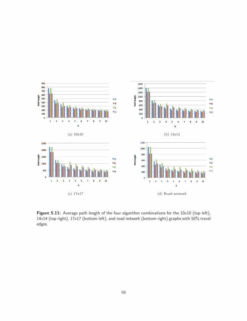
(a) 10x10 (b) 14x14

(c) 17x17 (d) Road network

Figure 5.11: Average path length of the four algorithm combinations for the 10x10 (top left),14x14 (top right), 17x17 (bottom left), and road network (bottom right) graphs with 50% traveledges.

66

(a) 10x10 (b) 14x14

(c) 17x17 (d) Road network

Figure 5.12: Average path variance of the four algorithm combinations for the 10x10 (topleft), 14x14 (top right), 17x17 (bottom left), and road network (bottom right) graphs with50% travel edges.

Figure 5.13: Average path length of thefour algorithm combinations for the dynamictests with five replans for each set of edgeremovals.

Figure 5.14: Computation time for each al-gorithm in the dynamic tests.

67

variety in the degree of its vertices resulting in more distinct coverage clusters. The k-means

algorithm is better at finding these clusters.

From the path variance results shown in Figure 5.12, algorithms A and B do much better than

algorithms C and D in terms of generating paths with more consistent costs – in some cases, the

variance is half the variance of C and D such as on the road network graph with six robots. On

average, algorithms A and B have path variances of 0.18, and algorithms C and D have variances

of 0.32. This shows that our approach is more successful in generating paths with similar costs,

and that the lower variance is due to the k-means method. However, in certain cases, algorithm

A performs better than algorithm B, such as for the trial with the 17x17 graph with five robots.

This indicates that while the use of travel edges in computing the route reduces the maximum

cost path, it can also have the side effect of increasing the variation between the k paths.

Dynamic k-RPP Tests

In the dynamic tests shown in Figure 5.13, our k-RPP algorithm (B) finds the lowest cost paths as

well. Because each algorithm produces different paths initially, the revised graph at each replan

will vary for the four heuristics. As a result, algorithm B does not perform as well as it does

in the static case since the updated graphs will have different sets of coverage and travel edges.

This test shows that in spite of the variations in graphs, our k-RPP still performs the best.

Figure 5.14 shows that the original k-RPP algorithm has the lowest runtime while our k-RPP

algorithm has the highest runtime. Of the two improvements, k-means is the more expensive.

However, for the sizes of the graphs we used, the computation times for the improved algorithm

are reasonable. Finally, Table 5.3 shows that, on average, the graphs used for the dynamic tests

were roughly the same as the graphs used for the static tests where half the edges in the graph

are travel and half are coverage.

Discussion

The results show that our k-RPP algorithm does find shorter maximum paths, which translates to

a shorter traversal time for robot teams of differing sizes. Our static tests show that our algorithm

can produce paths that are lower than those generated by the original algorithm as well as paths

that are more similar in cost. While the sole use of k-means enables a more even distribution

between the costs of the paths as well as lower path costs, including travel edges in the CPP

algorithm helps further decrease the cost of the worst performing path. The combination of the

two algorithms led to a better set of paths overall. Moreover, the improved k-RPP algorithm

is robust to graph discrepancies as the dynamic tests demonstrate. Of the two improvements,

k-means is more effective when the value of k is larger than four while using travel edges is better

when k is lower than four.

From the timing results, we can see that k-means clustering is more computationally costly

to use than including travel edges. Despite being more costly, replans still take less than a second

68

on the rectilinear graphs and one and a half seconds on the large road network. However, if

computation resources are limited, one strategy is to always include the travel edge improvement

since it is inexpensive; when planning offline, the algorithm would use both improvements, and

when replanning online, it would exclude the k-means clustering. Additionally, we chose to limit

the number of iterations of k-means at 100, but this number could be lowered to decrease the

computation time.

5.2 Route First, Cluster Second Approach

So far, we have described a C1R2 approach. We also looked into a R1C2 approach. In this

framework, the k-RPP problem is cast as a RPP problem and a solution is computed. The next

step is to divide the solution into k segments for each of the robots. For the division process, we

use an algorithm introduced for the Min Max k-CPP problem [Frederickson et al., 1976b]. We

call this algorithm FHK, and it operates in the following manner. The FHK algorithm begins

with a tour s...s where s is the depot vertex. Next, it partitions the tour into k sections with

similar cost: {(s...v1), (v2...v3), ..., (vk...s)} where vi is a vertex along the path. Finally the path

segments are modified to begin and end at s by adding a shortest path segment from vi to s or

from s to vi when needed. Moreover, it generates a (2 − 1k)-optimal approximation if the initial

RPP path is optimal.

We present two approximate algorithms that differ in the computation of the RPP. The first

uses an approximation algorithm for the RPP. The second uses the optimal algorithm for the

RPP that was presented in the previous chapter.

5.2.1 k-RPP Approximation: Approximation Algorithm for RPP

The first approximation algorithm consists of calling two bounded approximation methods in

sequence. The first method uses Frederickson’s 32 -optimal approximation for the RPP as detailed

in [Eiselt et al., 1995b]. Since the second method used is the (2 − 1k)-optimal path division

algorithm, the total heuristic gives (3 − 32k ) approximation factor on the optimal solution to the

k-RPP. When k is one, the 3/2-optimal bound is maintained, but can go up to three times the

optimal when k is large.

The RPP approximation algorithm consists of two steps. First, it computes the set of travel

edges that need to be added to the graph. To do this, we generate a Minimum Spanning Tree

(MST) shown in Algorithm 10. The MST is computed using Kruskal’s algorithm [Kruskal, 1956]

which uses a union-find method to track the affinity of vertices to connected components. First,

the connected coverage components from the original graph are computed. Each component

becomes a vertex in a condensed graph (lines 1 and 2). Edges are added to the condensed graph,

G′, that represent the shortest paths between the vertices in the different components (line 3).

Next, the edges are added to a priority queue (line 4). While the priority queue is not empty, an

69

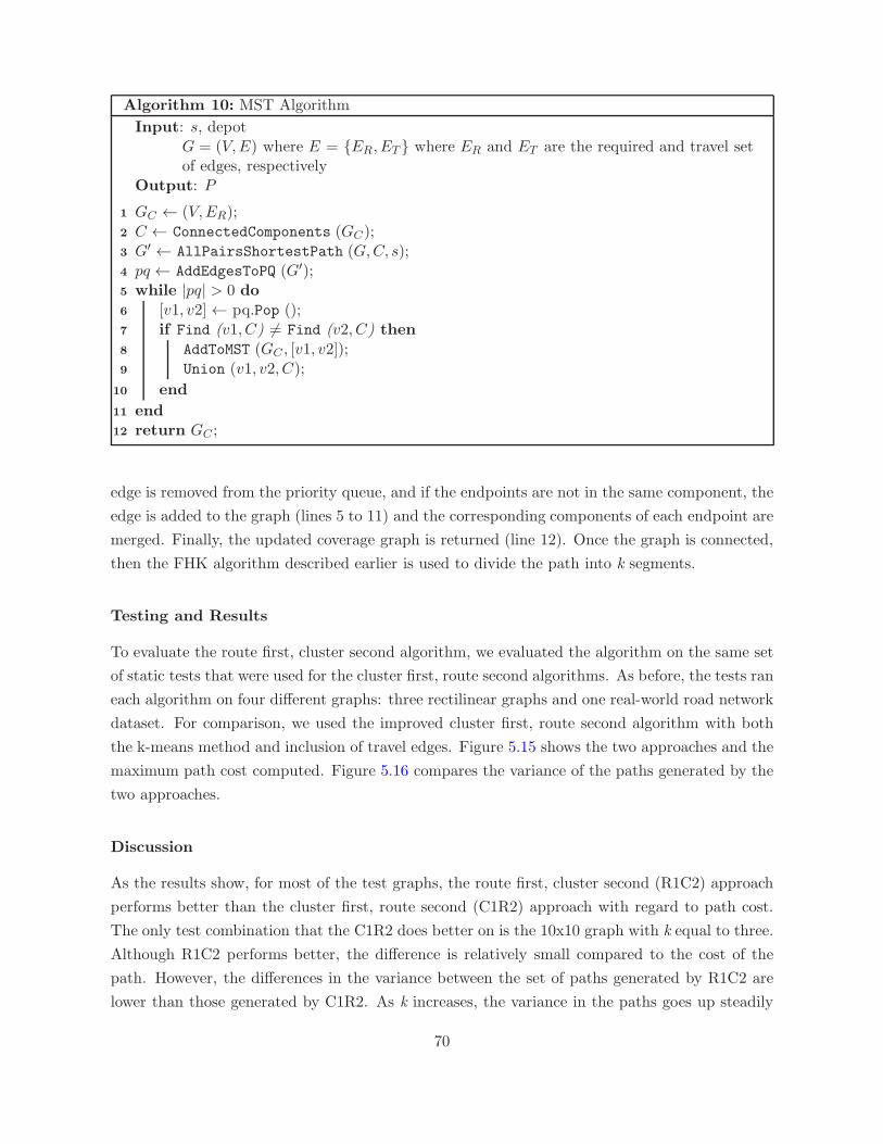
Algorithm 10: MST Algorithm

Input: s, depotG = (V,E) where E = {ER, ET } where ER and ET are the required and travel setof edges, respectively

Output: P

1 GC ← (V,ER);2 C ← ConnectedComponents (GC);3 G′ ← AllPairsShortestPath (G,C, s);4 pq ← AddEdgesToPQ (G′);5 while |pq| > 0 do6 [v1, v2] ← pq.Pop ();7 if Find (v1, C) 6= Find (v2, C) then8 AddToMST (GC , [v1, v2]);9 Union (v1, v2, C);

10 end

11 end12 return GC ;

edge is removed from the priority queue, and if the endpoints are not in the same component, the

edge is added to the graph (lines 5 to 11) and the corresponding components of each endpoint are

merged. Finally, the updated coverage graph is returned (line 12). Once the graph is connected,

then the FHK algorithm described earlier is used to divide the path into k segments.

Testing and Results

To evaluate the route first, cluster second algorithm, we evaluated the algorithm on the same set

of static tests that were used for the cluster first, route second algorithms. As before, the tests ran

each algorithm on four different graphs: three rectilinear graphs and one real-world road network

dataset. For comparison, we used the improved cluster first, route second algorithm with both

the k-means method and inclusion of travel edges. Figure 5.15 shows the two approaches and the

maximum path cost computed. Figure 5.16 compares the variance of the paths generated by the

two approaches.

Discussion

As the results show, for most of the test graphs, the route first, cluster second (R1C2) approach

performs better than the cluster first, route second (C1R2) approach with regard to path cost.

The only test combination that the C1R2 does better on is the 10x10 graph with k equal to three.

Although R1C2 performs better, the difference is relatively small compared to the cost of the

path. However, the differences in the variance between the set of paths generated by R1C2 are

lower than those generated by C1R2. As k increases, the variance in the paths goes up steadily

70

(a) 10x10 (b) 14x14

(c) 17x17 (d) Road network

Figure 5.15: Average path length of the C1R2 heuristics versus the R1C2 heuristic for the10x10 (top left), 14x14 (top right), 17x17 (bottom left), and road network (bottom right)graphs with 50% travel edges.

for the R1C2. For the C1R2 algorithm, the variance is more erratic, but overall the trend goes

up proportional to k.

The R1C2 algorithm performs better both in path cost and variance because its initial gen-

eration of a path helps to minimize the set of travel edges used, and the path division algorithm

effectively splits the path such that the cost of each segment is relatively equal among the mem-

bers of the team. On the other hand, while the clustering step in the C1R2 algorithm may divide

the edges evenly among the team, this initially fair distribution may not translate to similar cost

routes generated for each cluster.

5.2.2 k-RPP Approximation: Optimal Algorithm for RPP

The second heuristic algorithm that we present for the k-RPP computes an optimal route first

for the RPP and then divides it using the FHK method. As a result, this algorithm has an

approximation factor of (2 − 1k). As k gets larger, the bound gets closer to two times optimal.

71

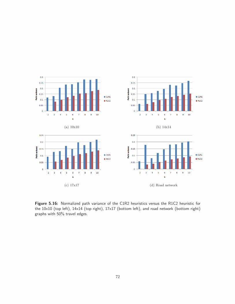
(a) 10x10 (b) 14x14

(c) 17x17 (d) Road network

Figure 5.16: Normalized path variance of the C1R2 heuristics versus the R1C2 heuristic forthe 10x10 (top left), 14x14 (top right), 17x17 (bottom left), and road network (bottom right)graphs with 50% travel edges.

72

Figure 5.17: The normalized value and standard deviation of the variation of k path costs.Each value represents the average over k where k ranges from two to four.

Since the routing step is the more expensive portion of the algorithm, we focus on minimizing

the computation time for the search. This will, in turn, minimize the total computation time for

the k-RPP problem.

Finding an optimal RPP solution can be expensive. One way to overcome this is to use

the parallel branch-and-bound framework presented in the previous chapter. For multi-robot

problems, each robot is assumed to contain a separate processor. Team members communicate

over a wireless network. This setup makes use of the entire robot team to expedite the search

problem.

Testing and Results

The tests for this algorithm were similar to the tests used in section 4.4.2. The only addition

was the call to the FHK method to divide the optimal path into k routes. The same results from

the previous testing hold for this set of tests. To evaluate the performance of this algorithm, we

focus on the set of paths generated.

For the k-RPP problem, we are trying to minimize the maximum or worst cost path for k

robots. The goal of the MinMax objective is to better distribute the work and reduce the total

traversal time for the team. As a result, we computed the path variation of the k generated

paths. Figure 5.17 shows the variation of the paths normalized by the mean of the paths. This

value is averaged over all values of k. As shown, the variation is fairly low for the different

graphs. By using an optimal algorithm, the solution includes the minimum set of optional edges.

Furthermore, the route division process is bounded which ensures that few extraneous edges are

added. As a result, the final solution is a set of paths that are highly similar in cost.

This work comprises a first implementation of an optimal market solution for coupled robot

73

systems where a combinatorial optimization technique, the branch-and-bound algorithm, is paral-

lelized for a team of robots. It is combined with an auction framework between the robots to solve

large coverage problems more efficiently. As the results show, the market-based approach helps

divide the solution space of the coverage problem among multiple robots, but allows the robots to

still access the entire space through the use of auctions. These techniques enable multiple robots

to generate a bounded solution for the k-RPP through working together.

While our experiments did not model this scenario, this distributed auction system can be

extended in cases where communication fails between the robots by making minor modifications

to the algorithm. When robots cannot share information with each other, the ability of the

system to find an optimal solution to the RPP problem is compromised. To tackle this situation,

when the robots realize they are no longer in contact, each group of robots still connected must

switch from working on the part of the search tree they were assigned to also working on the

remaining parts of the tree to which the disconnected robots are computing. In essence, the

individual groups of robots still in communication must recreate the entire search tree themselves

and perform the extra work required to find the optimal solution. More details of this strategy

are discussed in Appendix C.

5.3 Conclusion

This chapter addressed the partial coverage problem with multiple robots. Based on the op-

erational research literature, this problem is cast as a k-Rural Postman problem. Solving this

problem optimally is not ideal for fast planning and replanning. Two heuristic approaches were

proposed. The first, a cluster first, route second, approach is an improved version of the only

existing algorithm for this problem. Our improved algorithm used k-means to cluster the graph

edges and travel edges to generate shorter routes. Through the two modifications, the algorithm

performs better by returning lower cost paths and less variation within the path costs. The second

approach is a route first, cluster second approach which uses two bounded heuristic algorithms

to solve this problem. From our tests, the second approach performs better than the first in

generating lower cost and less variable solutions.

While these heuristics provide efficient algorithms for the real-time robotic operation, they do

not provide high quality solutions. Another version of the route first, cluster second algorithm

was introduced that uses an optimal algorithm to find the initial route. To increase efficiency, this

algorithm uses the parallel branch-and-bound algorithm to generate the optimal solution. This

approach demonstrates the extension of the parallel branch-and-bound framework to a team of

robots.

74

Chapter 6

Partial Coverage with Multiple

Robots with Environmental

Constraints

This chapter addresses the most general of the coverage problems presented in this thesis. This

coverage problem is also the most complex since it incorporates all the problem dimensions:

partial coverage, multiple robots, environmental constraints, and replanning. The addition of

directionality constraints in the form of arcs allows the coverage problem to model more practical

environments and applications. This problem can be framed as the k-Mixed Chinese Postman

problem and the k-Mixed Rural Postman problem.

For the coverage problems discussed in the previous chapters, the branch-and-bound approach

has been used to address the whole problem or a part of the problem. This optimal algorithm

produces solutions relatively efficiently because the subproblems are polynomial-time. When

multiple robots and arcs are added to the coverage problem, the problem becomes more complex

given the two extra dimensions added to an already NP-hard problem of partial coverage. The

branch-and-bound technique is not sufficient anymore because every node of the tree would

now contain an NP-hard problem with no polynomial-time solution. In this case, finding an

optimal solution is computationally expensive and infeasible for the real-time tasks that this

work addresses.

For this class of problems, we do not expect to generate optimal solutions, and focus instead

on approximate solutions using heuristics. In general, we still follow the same paradigm of using

lower complexity algorithms to solve more complex problems by breaking the problem down into

its different dimensions. In this manner, we can focus on each dimension of the problem separately

through a reduction process. The problem of partial coverage in an environment with edges and

arcs with multiple robots can be solved by first factoring out and solving the multiple robot

problem independently. This reduces the problem to partial coverage in an environment with

75

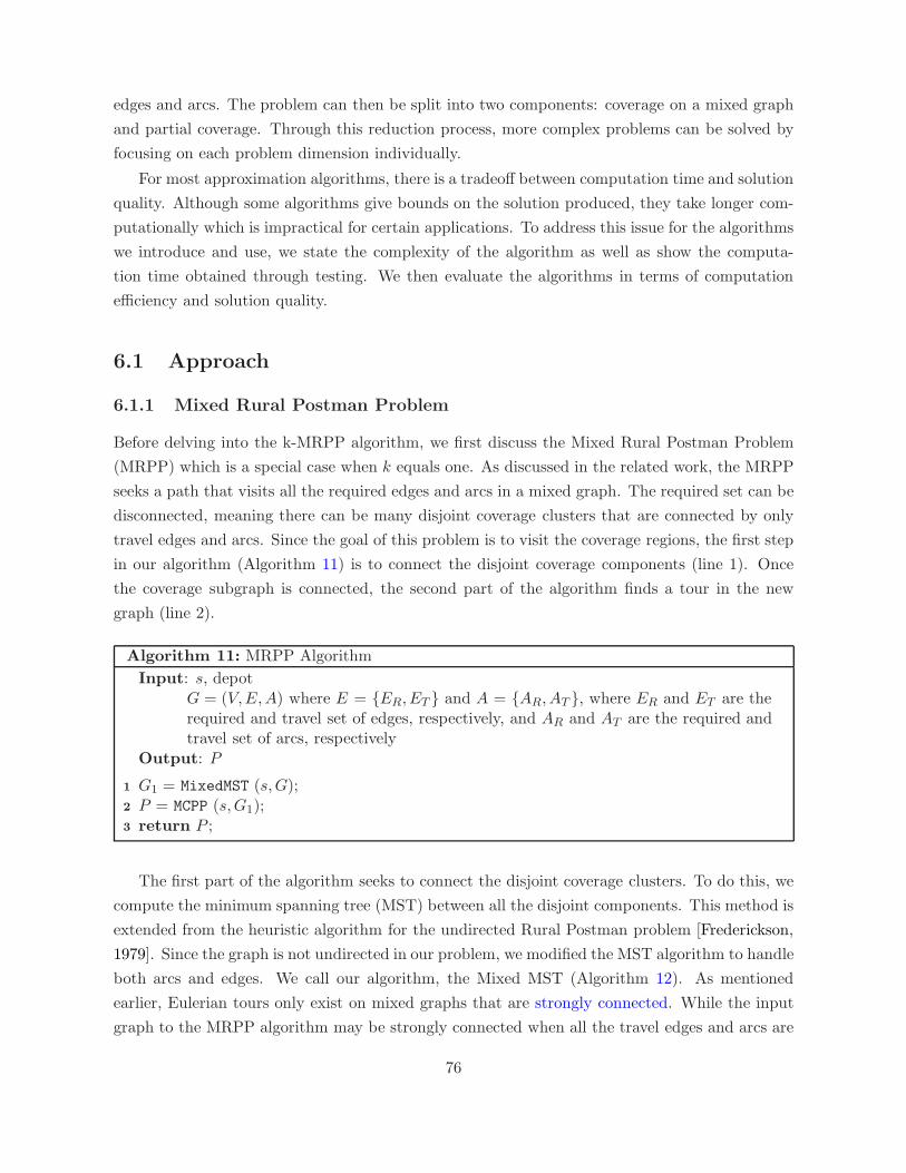
edges and arcs. The problem can then be split into two components: coverage on a mixed graph

and partial coverage. Through this reduction process, more complex problems can be solved by

focusing on each problem dimension individually.

For most approximation algorithms, there is a tradeoff between computation time and solution

quality. Although some algorithms give bounds on the solution produced, they take longer com-

putationally which is impractical for certain applications. To address this issue for the algorithms

we introduce and use, we state the complexity of the algorithm as well as show the computa-

tion time obtained through testing. We then evaluate the algorithms in terms of computation

efficiency and solution quality.

6.1 Approach

6.1.1 Mixed Rural Postman Problem

Before delving into the k-MRPP algorithm, we first discuss the Mixed Rural Postman Problem

(MRPP) which is a special case when k equals one. As discussed in the related work, the MRPP

seeks a path that visits all the required edges and arcs in a mixed graph. The required set can be

disconnected, meaning there can be many disjoint coverage clusters that are connected by only

travel edges and arcs. Since the goal of this problem is to visit the coverage regions, the first step

in our algorithm (Algorithm 11) is to connect the disjoint coverage components (line 1). Once

the coverage subgraph is connected, the second part of the algorithm finds a tour in the new

graph (line 2).

Algorithm 11: MRPP Algorithm

Input: s, depotG = (V,E,A) where E = {ER, ET } and A = {AR, AT }, where ER and ET are therequired and travel set of edges, respectively, and AR and AT are the required andtravel set of arcs, respectively

Output: P

1 G1 = MixedMST (s,G);2 P = MCPP (s,G1);3 return P ;

The first part of the algorithm seeks to connect the disjoint coverage clusters. To do this, we

compute the minimum spanning tree (MST) between all the disjoint components. This method is

extended from the heuristic algorithm for the undirected Rural Postman problem [Frederickson,

1979]. Since the graph is not undirected in our problem, we modified the MST algorithm to handle

both arcs and edges. We call our algorithm, the Mixed MST (Algorithm 12). As mentioned

earlier, Eulerian tours only exist on mixed graphs that are strongly connected. While the input

graph to the MRPP algorithm may be strongly connected when all the travel edges and arcs are

76

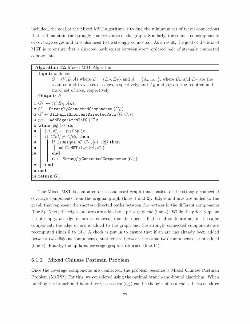
included, the goal of the Mixed MST algorithm is to find the minimum set of travel connections

that still maintain the strongly connectedness of the graph. Similarly, the connected components

of coverage edges and arcs also need to be strongly connected. As a result, the goal of the Mixed

MST is to ensure that a directed path exists between every ordered pair of strongly connected

components.

Algorithm 12: Mixed MST Algorithm

Input: s, depotG = (V,E,A) where E = {ER, ET } and A = {AR, AT }, where ER and ET are therequired and travel set of edges, respectively, and AR and AT are the required andtravel set of arcs, respectively

Output: P

1 GC ← (V,ER, AR);2 C ← StronglyConnectedComponents (GC);3 G′ ← AllPairsShortestDirectedPath (G,C, s);4 pq ← AddEdgesArcsToPQ (G′);5 while |pq| > 0 do6 [v1, v2] ← pq.Pop ();7 if C[v1] 6= C[v2] then8 if IsUnique (C,GC , [v1, v2]) then9 AddToMST (GC , [v1, v2]);

10 end11 C ← StronglyConnectedComponents (GC);

12 end

13 end14 return GC ;

The Mixed MST is computed on a condensed graph that consists of the strongly connected

coverage components from the original graph (lines 1 and 2). Edges and arcs are added to the

graph that represent the shortest directed paths between the vertices in the different components

(line 3). Next, the edges and arcs are added to a priority queue (line 4). While the priority queue

is not empty, an edge or arc is removed from the queue. If the endpoints are not in the same

component, the edge or arc is added to the graph and the strongly connected components are

recomputed (lines 5 to 13). A check is put in to ensure that if an arc has already been added

between two disjoint components, another arc between the same two components is not added

(line 8). Finally, the updated coverage graph is returned (line 14).

6.1.2 Mixed Chinese Postman Problem

Once the coverage components are connected, the problem becomes a Mixed Chinese Postman

Problem (MCPP). For this, we considered using the optimal branch-and-bound algorithm. When

building the branch-and-bound tree, each edge (i, j) can be thought of as a choice between three

77

types of arc sets: {i → j}, {j → i}, and {i → j, j → i}. Each branch in the search tree

would consist of these three choices, and each subproblem could be solved as a Directed Chinese

Postman problem (see Appendix A). While this method generates the optimal solution for the

MCPP, it is computationally prohibitive to use. As a result, we chose to use an existing heuristic

algorithm to solve this problem.

An existing algorithm by Frederickson and subsequent improvements by Raghavachari and

Veerasamy solve the MCPP heuristically [Frederickson, 1979][Raghavachari and Veerasamy, 1998].

A mixed graph contains an Eulerian tour if it is both even and balanced. Since finding a balanced

graph can be difficult, Frederickson uses the more general approach of making the graph even

and symmetric.

The MCPP algorithm consists of two main methods, Mixed1 and Mixed2, which take two

complementary approaches to solving this problem. Figure 6.1 shows the methods used in the

original MCPP algorithm. Mixed1 first ensures the graph is even and then symmetric. The first

function EvenDegree copies the input graph and converts every arc to an edge. Next, it adds

the minimum cost matching generated on this copy to the original graph effectively transforming

all the vertices to even. Next, the graph is augmented to be symmetric using the minimum cost

maximum flow method in the InOutDegree function. More details on this are given later. Since

the InOutDegree function may have converted some vertices to be odd, the EvenParity function

is used to restore those vertices back to an even degree. Finally, a tour is computed on the

augmented graph and the cost of the tour is returned. For Mixed2, the goal is to make the graph

symmetric, then even. Making the graph symmetric is done by using the InOutDegree function.

The graph is then transformed into an even graph by adding a minimum cost matching that is

based only on the edges in the graph. A solution is computed and the cost is returned. The lower

cost of the solutions returned by Mixed1 and Mixed2 is the final solution for the MCPP.

This original algorithm generates a bounded solution that is 53 times optimal. It was improved

to a tighter bound by the improved MCPP algorithm shown in Figure 6.2. To accomplish this, the

InOutDegree function is first called on the input graph. Mixed2 stays the same. The algorithm

for Mixed1 changes slightly. Let the set of arcs and converted edges in the graph returned by

InOutDegree be denoted by M . The same arcs and edges in the original graph that correspond

to those in M are set to a cost of zero, and then the remainder of Mixed1 is run as before.

Through this change, methods Mixed1 and Mixed2 return the same bound for disjoint halves of

the solution space. Therefore, by selecting the minimum cost of the solutions returned by Mixed1

and Mixed2, the MCPP algorithm guarantees a solution that is at most 32 times optimal.

While the other methods are relatively straightforward, we go into more details about the

InOutDegree method. The method InOutDegree, shown in Alg. 13, augments the graph with

additional edges and arcs to make it symmetric. To do so, it converts some of the existing edges

into arcs and adds additional arcs and edges. In order to use the minimum cost maximum flow

method which only operates on directed graphs, we transform the original graph into a new graph

78

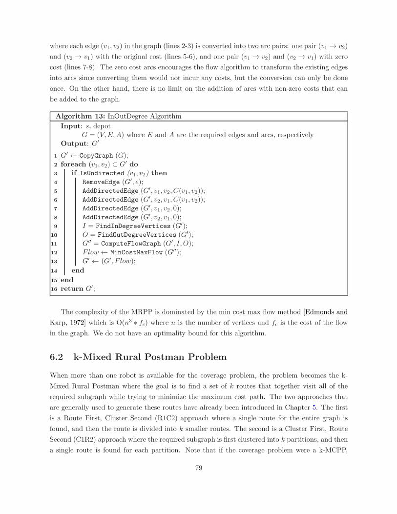
where each edge (v1, v2) in the graph (lines 2-3) is converted into two arc pairs: one pair (v1 → v2)

and (v2 → v1) with the original cost (lines 5-6), and one pair (v1 → v2) and (v2 → v1) with zero

cost (lines 7-8). The zero cost arcs encourages the flow algorithm to transform the existing edges

into arcs since converting them would not incur any costs, but the conversion can only be done

once. On the other hand, there is no limit on the addition of arcs with non-zero costs that can

be added to the graph.

Algorithm 13: InOutDegree Algorithm

Input: s, depotG = (V,E,A) where E and A are the required edges and arcs, respectively

Output: G′

1 G′ ← CopyGraph (G);2 foreach (v1, v2) ⊂ G′ do3 if IsUndirected (v1, v2) then4 RemoveEdge (G′, e);5 AddDirectedEdge (G′, v1, v2, C(v1, v2));6 AddDirectedEdge (G′, v2, v1, C(v1, v2));7 AddDirectedEdge (G′, v1, v2, 0);8 AddDirectedEdge (G′, v2, v1, 0);9 I = FindInDegreeVertices (G′);

10 O = FindOutDegreeVertices (G′);11 G′′ = ComputeFlowGraph (G′, I, O);12 Flow ← MinCostMaxFlow (G′′);13 G′ ← (G′, F low);

14 end

15 end16 return G′;

The complexity of the MRPP is dominated by the min cost max flow method [Edmonds and

Karp, 1972] which is O(n3 ∗ fc) where n is the number of vertices and fc is the cost of the flow

in the graph. We do not have an optimality bound for this algorithm.

6.2 k-Mixed Rural Postman Problem

When more than one robot is available for the coverage problem, the problem becomes the k-

Mixed Rural Postman where the goal is to find a set of k routes that together visit all of the

required subgraph while trying to minimize the maximum cost path. The two approaches that

are generally used to generate these routes have already been introduced in Chapter 5. The first

is a Route First, Cluster Second (R1C2) approach where a single route for the entire graph is

found, and then the route is divided into k smaller routes. The second is a Cluster First, Route

Second (C1R2) approach where the required subgraph is first clustered into k partitions, and then

a single route is found for each partition. Note that if the coverage problem were a k-MCPP,

79

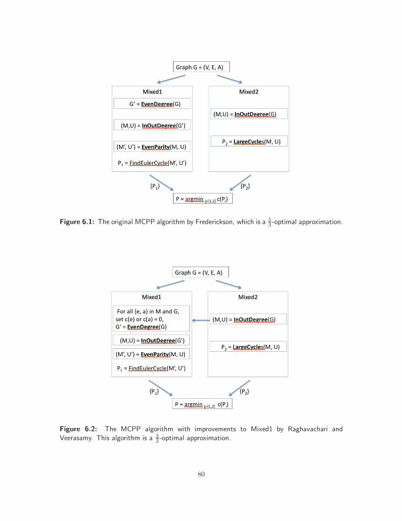
Figure 6.1: The original MCPP algorithm by Frederickson, which is a 53 -optimal approximation.

Figure 6.2: The MCPP algorithm with improvements to Mixed1 by Raghavachari andVeerasamy. This algorithm is a 3

2 -optimal approximation.

80

then we can just use the bounded algorithm for the MCPP to substitute for the MRPP method

calls.

Next, we discuss each of the approaches in detail and how they are framed for our problem.

6.2.1 Route First, Cluster Second Approach

The R1C2 approach consists of two steps (Algorithm 14). Step one simplifies the problem by

assuming k equals one. As a result, the problem becomes the MRPP, and a solution can be found

using the MRPP algorithm that we introduced earlier (line 1). Next, the solution is split into k

routes by using the FHK algorithm [Frederickson et al., 1976b] (line 2).

This algorithm is dominated by the MRPP and therefore has the same complexity. If an

optimal algorithm for the MRPP was used as part of this approach, then it can generate a

(2 − 1k)-optimal solution but will have an exponential complexity due to solving the NP-hard

MRPP problem optimally.

Algorithm 14: Route First, Cluster Second Algorithm for the k-MRPP

Input: s, depotG = (V,E,A) where E = {ER, ET } and A = {AR, AT }, where ER and ET are therequired and travel set of edges, respectively, and AR and AT are the required andtravel set of arcs, respectively

Output: P

1 P ← MRPP (G, s);2 P1...k ← FHK (G,P, s);3 return P1...k;

6.2.2 Cluster First, Route Second Approach

The C1R2 approach also consists of two main steps (Algorithm 15). This algorithm is an extended

version of the k-RPP method discussed in the previous chapter. In the algorithm, the first step

separates the required subgraph into k portions using the k-means method [MacQueen, 1967]

(lines 1 and 2). The goal of k-means is to maximize the distance between the centers of the

different clusters and minimize the distance between required edges and arcs within each cluster.

After the graph is divided into the k clusters, the algorithm finds a route for every cluster by

calling the MRPP algorithm. Note that the edges and arcs within a cluster may not be connected

after the clustering step. To handle this situation, for each cluster, we subtract the required edges

and arcs from the original set of arcs and edges. We include the remainder as travel edges in

the graphs Gi for each cluster i (lines 4 to 6). Next, the algorithm calls the MRPP algorithm

on Gi and a path is returned for robot i (line 7). Finally, all k paths are returned (line 9). This

algorithm has the same worst case complexity as the MRPP.

81

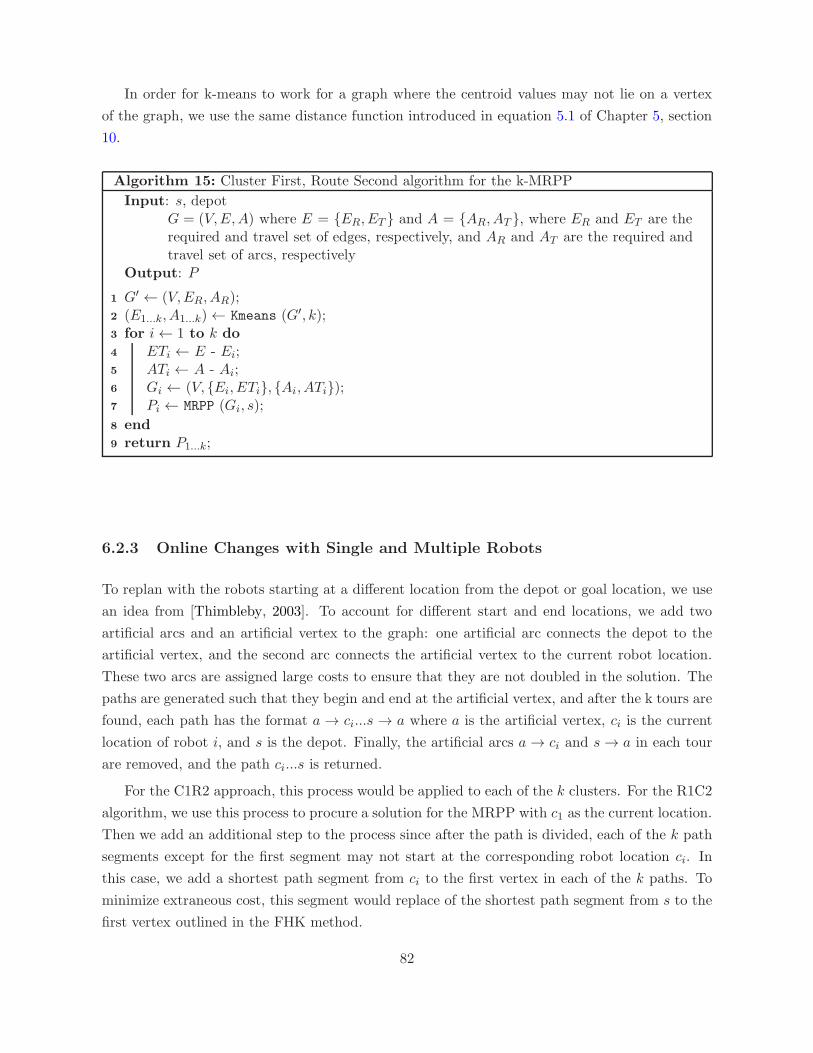
In order for k-means to work for a graph where the centroid values may not lie on a vertex

of the graph, we use the same distance function introduced in equation 5.1 of Chapter 5, section

10.

Algorithm 15: Cluster First, Route Second algorithm for the k-MRPP

Input: s, depotG = (V,E,A) where E = {ER, ET } and A = {AR, AT }, where ER and ET are therequired and travel set of edges, respectively, and AR and AT are the required andtravel set of arcs, respectively

Output: P

1 G′ ← (V,ER, AR);2 (E1...k, A1...k)← Kmeans (G′, k);3 for i← 1 to k do4 ETi ← E - Ei;5 ATi ← A - Ai;6 Gi ← (V, {Ei, ETi}, {Ai, ATi});7 Pi ← MRPP (Gi, s);

8 end9 return P1...k;

6.2.3 Online Changes with Single and Multiple Robots

To replan with the robots starting at a different location from the depot or goal location, we use

an idea from [Thimbleby, 2003]. To account for different start and end locations, we add two

artificial arcs and an artificial vertex to the graph: one artificial arc connects the depot to the

artificial vertex, and the second arc connects the artificial vertex to the current robot location.

These two arcs are assigned large costs to ensure that they are not doubled in the solution. The

paths are generated such that they begin and end at the artificial vertex, and after the k tours are

found, each path has the format a → ci...s → a where a is the artificial vertex, ci is the current

location of robot i, and s is the depot. Finally, the artificial arcs a→ ci and s→ a in each tour

are removed, and the path ci...s is returned.

For the C1R2 approach, this process would be applied to each of the k clusters. For the R1C2

algorithm, we use this process to procure a solution for the MRPP with c1 as the current location.

Then we add an additional step to the process since after the path is divided, each of the k path

segments except for the first segment may not start at the corresponding robot location ci. In

this case, we add a shortest path segment from ci to the first vertex in each of the k paths. To

minimize extraneous cost, this segment would replace of the shortest path segment from s to the

first vertex outlined in the FHK method.

82

6.3 Testing Framework

Our testing compared the two versions of k-MRPP algorithm, both of which utilize the MRPP

heuristic. We conducted two sets of tests: static and dynamic k-MRPP tests. The first set of tests

evaluated the two multi-robot approaches, C1R2 and R1C2, on several sets of graphs. The second

test set assesses the replanning capability of the algorithm when handling online changes. For

each test, we varied four different parameters: algorithm, graph, starting vertex s, and number of

robots k. The tests were simulated with k robots executing k tours starting at vertex s. The code

ran on a machine with a 2.53GHz Intel processor and 4GB of RAM. For the testing framework,

we will first explain the test graphs, then the procedure for each test, and finally present the

metrics for performance evaluation.

6.3.1 Test Graphs

For our tests, we utilized two sets of graphs: rectilinear graphs and a physical road network (shown

in Appendix B). For the rectilinear graphs, three graph sizes were used: {10×10, 14×14, 17×17}.

For both the rectilinear and physical road graphs, a random set of edges were selected to be arcs.

6.3.2 Static k-MRPP Tests

The static k-MRPP tests ran each algorithm on twenty different graphs: fifteen distinct rectilinear

graphs (five for each graph size) and five road network graphs. For each graph, we varied the

number of robots, k, from one to ten. For the rectilinear graphs and each k value, we varied the

starting vertex over a random set consisting of half of the vertices in the graph to avoid bias.

Therefore, both algorithms were called k × 3× 5× |V |2 times where |V | is the number of vertices

in the graph. For the road network, we sampled a set of fifty distinct vertices. The samples were

consistent for both approaches, and this test yielded k × 5× 50 plans for each algorithm.

6.3.3 Dynamic Tests

For the second set of tests, our goal was to evaluate the performance of both k-MRPP algorithms

in replanning online when changes occur. For these tests, we add a new parameter, a set of

changes. Additionally, we constrained k to be ten. At the beginning of the test, the graph is

connected and has no travel edges or arcs. Using the coverage algorithm, ten tours are computed.

Each trial simulates the robots executing the tours starting at vertex s. If along the execution,

the next edge or arc to be traversed is in the change set, that edge or arc is considered blocked.

It is removed from the graph, and the graph is updated to reflect the visited edges and arcs and

current robot locations. Using the updated graph, the algorithm plans a new set of tours. The

execution is simulated again until another edge or arc along the new path is found to be blocked

or the traversal is completed. This test consisted of 3×5× |V |2 +5×50 replans for each approach.

83

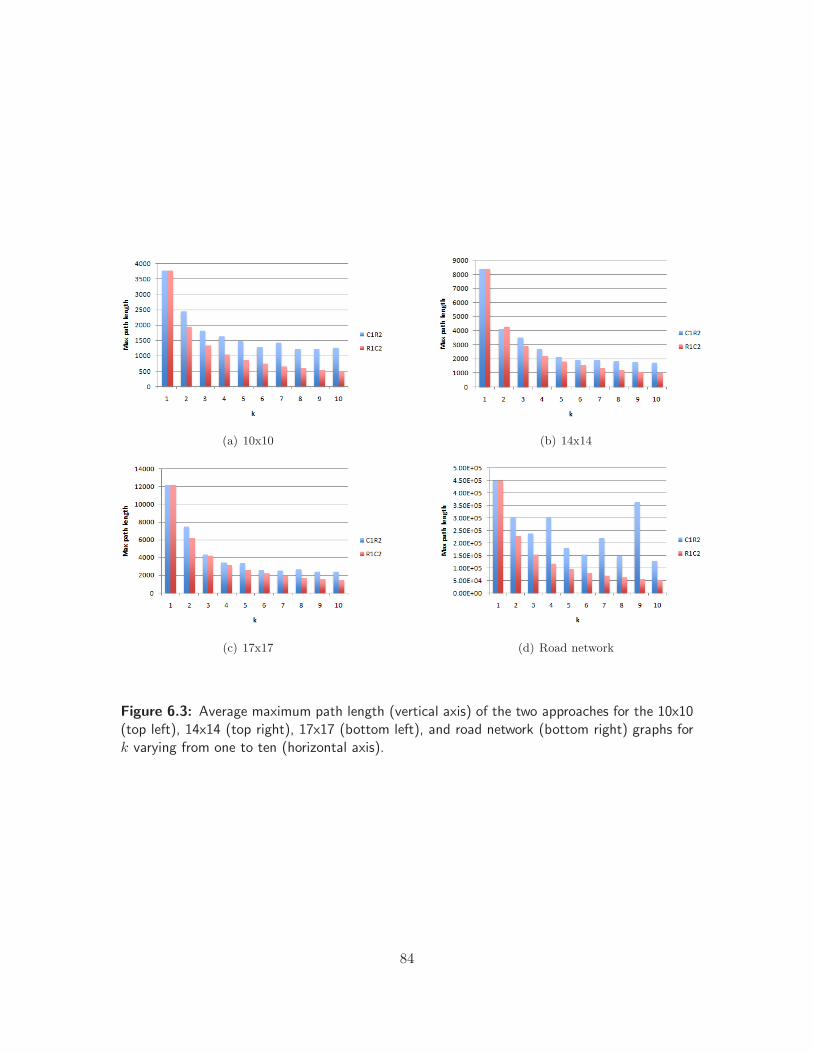
(a) 10x10 (b) 14x14

(c) 17x17 (d) Road network

Figure 6.3: Average maximum path length (vertical axis) of the two approaches for the 10x10(top left), 14x14 (top right), 17x17 (bottom left), and road network (bottom right) graphs fork varying from one to ten (horizontal axis).

84

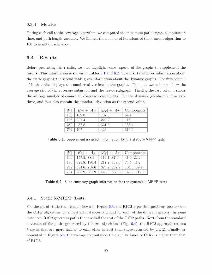
6.3.4 Metrics

During each call to the coverage algorithm, we computed the maximum path length, computation

time, and path length variance. We limited the number of iterations of the k-means algorithm to

100 to maintain efficiency.

6.4 Results

Before presenting the results, we first highlight some aspects of the graphs to supplement the

results. This information is shown in Tables 6.1 and 6.2. The first table gives information about

the static graphs; the second table gives information about the dynamic graphs. The first column

of both tables displays the number of vertices in the graphs. The next two columns show the

average size of the coverage subgraph and the travel subgraph. Finally, the last column shows

the average number of connected coverage components. For the dynamic graphs, columns two,

three, and four also contain the standard deviation as the second value.

|V | |ER| + |AR| |ET | + |AT | Components

100 162.8 107.6 54.4

196 321.4 220.2 115

289 487.8 321.6 155.4

764 707 423 316.2

Table 6.1: Supplementary graph information for the static k-MRPP tests

|V | |ER| + |AR| |ET | + |AT | Components

100 157.5, 88.1 114.1, 87.0 41.0, 22.2

196 325.8, 170.4 217.2, 169.6 74.5, 41.2

289 484.6, 258.6 326.2, 257.7 104.6, 59.2

764 685.9, 361.9 445.3, 360.8 148.8, 119.3

Table 6.2: Supplementary graph information for the dynamic k-MRPP tests

6.4.1 Static k-MRPP Tests

For the set of static test results shown in Figure 6.3, the R1C2 algorithm performs better than

the C1R2 algorithm for almost all instances of k and for each of the different graphs. In some

instances, R1C2 generates paths that are half the cost of the C1R2 paths. Next, from the standard

deviation of the paths generated by the two algorithms (Fig. 6.4), the R1C2 approach returns

k paths that are more similar to each other in cost than those returned by C1R2. Finally, as

presented in Figure 6.5, the average computation time and variance of C1R2 is higher than that

of R1C2.

85

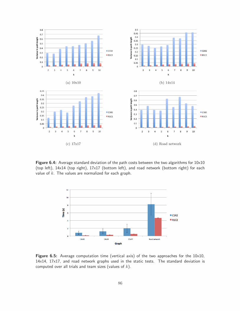
(a) 10x10 (b) 14x14

(c) 17x17 (d) Road network

Figure 6.4: Average standard deviation of the path costs between the two algorithms for 10x10(top left), 14x14 (top right), 17x17 (bottom left), and road network (bottom right) for eachvalue of k. The values are normalized for each graph.

Figure 6.5: Average computation time (vertical axis) of the two approaches for the 10x10,14x14, 17x17, and road network graphs used in the static tests. The standard deviation iscomputed over all trials and team sizes (values of k).

86

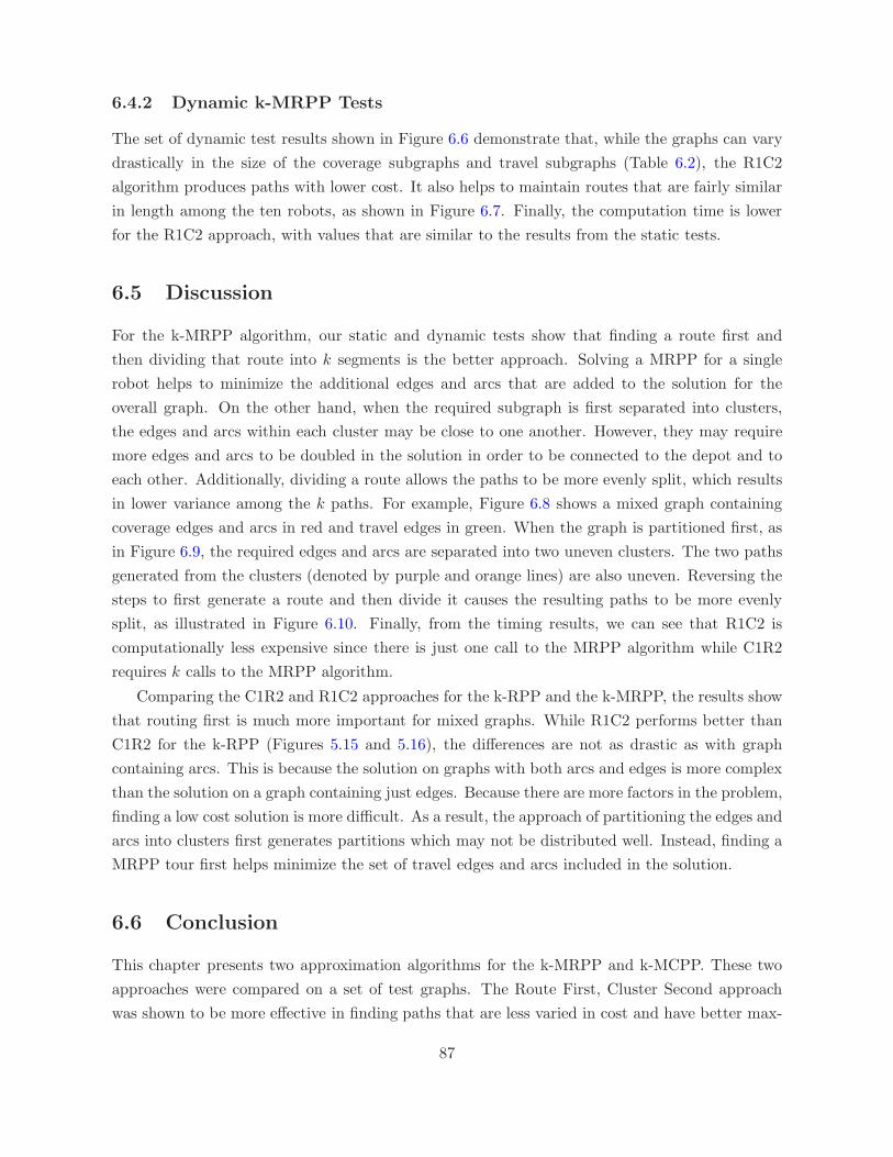
6.4.2 Dynamic k-MRPP Tests

The set of dynamic test results shown in Figure 6.6 demonstrate that, while the graphs can vary

drastically in the size of the coverage subgraphs and travel subgraphs (Table 6.2), the R1C2

algorithm produces paths with lower cost. It also helps to maintain routes that are fairly similar

in length among the ten robots, as shown in Figure 6.7. Finally, the computation time is lower

for the R1C2 approach, with values that are similar to the results from the static tests.

6.5 Discussion

For the k-MRPP algorithm, our static and dynamic tests show that finding a route first and

then dividing that route into k segments is the better approach. Solving a MRPP for a single

robot helps to minimize the additional edges and arcs that are added to the solution for the

overall graph. On the other hand, when the required subgraph is first separated into clusters,

the edges and arcs within each cluster may be close to one another. However, they may require

more edges and arcs to be doubled in the solution in order to be connected to the depot and to

each other. Additionally, dividing a route allows the paths to be more evenly split, which results

in lower variance among the k paths. For example, Figure 6.8 shows a mixed graph containing

coverage edges and arcs in red and travel edges in green. When the graph is partitioned first, as

in Figure 6.9, the required edges and arcs are separated into two uneven clusters. The two paths

generated from the clusters (denoted by purple and orange lines) are also uneven. Reversing the

steps to first generate a route and then divide it causes the resulting paths to be more evenly

split, as illustrated in Figure 6.10. Finally, from the timing results, we can see that R1C2 is

computationally less expensive since there is just one call to the MRPP algorithm while C1R2

requires k calls to the MRPP algorithm.

Comparing the C1R2 and R1C2 approaches for the k-RPP and the k-MRPP, the results show

that routing first is much more important for mixed graphs. While R1C2 performs better than

C1R2 for the k-RPP (Figures 5.15 and 5.16), the differences are not as drastic as with graph

containing arcs. This is because the solution on graphs with both arcs and edges is more complex

than the solution on a graph containing just edges. Because there are more factors in the problem,

finding a low cost solution is more difficult. As a result, the approach of partitioning the edges and

arcs into clusters first generates partitions which may not be distributed well. Instead, finding a

MRPP tour first helps minimize the set of travel edges and arcs included in the solution.

6.6 Conclusion

This chapter presents two approximation algorithms for the k-MRPP and k-MCPP. These two

approaches were compared on a set of test graphs. The Route First, Cluster Second approach

was shown to be more effective in finding paths that are less varied in cost and have better max-

87

Figure 6.6: Average maximum path cost (vertical axis) of the C1R2 and R1C2 approaches forthe 10x10, 14x14, 17x17, and road network graphs for five sets of online changes where k isten. The values for the road network have been scaled to fit.

Figure 6.7: Average standard deviation in length among the ten paths generated by the C1R2and R1C2 algorithms for the grid graphs and road graphs in the dynamic tests.

Figure 6.8: In this example, the graph is a mixed graph with arcs and edges. The red arcs/edgesare coverage and the green arcs/edges are travel.

88

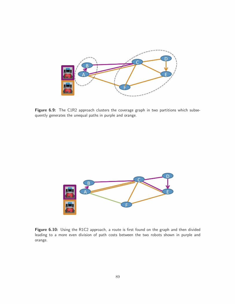
Figure 6.9: The C1R2 approach clusters the coverage graph in two partitions which subse-quently generates the unequal paths in purple and orange.

Figure 6.10: Using the R1C2 approach, a route is first found on the graph and then dividedleading to a more even division of path costs between the two robots shown in purple andorange.

89

imum cost paths. While we introduced a heuristic for the MRPP that is fast computationally,

it does not give any guarantees on solution quality. If the quality of the solution is important, a

better performing algorithm may be substituted to solve this problem. These algorithms include

constructive heuristic and tabu search methods suggested by [Corberan et al., 2000] or heuris-

tics for the Windy Rural Postman Problem [Benavent et al., 2003][Benavent et al., 2003]. As

demonstrated by the communication tests performed with the k-RPP (Appendix C), finding a

higher quality solution for part of the problem may translate to an overall solution that is lower in

cost. However, it is not guaranteed to always produce better solutions. Therefore, when deciding

on the algorithm, it is important to consider the trade-offs between computational efficiency or

solution quality within the context of the coverage application.

90

Chapter 7

Conclusion

7.1 Thesis Contributions

The approach presented in this thesis represents the first integrated planner that tackles the

multi-robot constrained coverage problem with environmental restrictions and replanning capa-

bilities. As discussed earlier, these coverage problems arise often in searching, mapping, and

patrolling applications. Our approach strives for optimal solutions when computation time is

flexible (namely, offline processing) and heuristic approximations when time is limited (which

often occurs when planning online in robotics applications).

We frame the coverage problem in constrained, network-like environments as an arc routing

problem where the environment is represented as a graph. To solve the multi-dimensional cov-

erage problem, the least complex problem is addressed first. The other dimensions are added to

the problem one by one and each resulting problem is modeled and addressed.

The contributions of this thesis are as follows:

1. The first coverage problem addressed is the partial coverage problem with replanning ca-

pabilities. This problem can be cast as a Rural Postman problem. We introduce a tractable,

optimal solution to this routing problem when the number of travel edges is small. The com-

plexity of the algorithm is O(v32t), where t is the number of travel edges and v is the number

of vertices in the graph. Additionally, we presented a novel path generation heuristic that helps

ensure graph connectivity as a way to maintain lower complexity replanning problems.

2. We introduce a parallel branch-and-bound approach that distributes the optimal solution

computation among multiple processes. Taking inspiration from market-based approaches, we

present a novel auction framework within the branch-and-bound approach for the processes to

share their individual search trees and avoid extraneous computation.

91

3. The second coverage problem tackled is the partial coverage problem with replanning capa-

bilities for a team of robots. This problem can be represented as a k-Rural Postman problem.

Since finding an optimal solution could be computationally costly, three heuristic approaches were

introduced: one Cluster First, Route Second approach, and two Route First, Cluster Second ap-

proaches. One version of the Route First, Cluster Second algorithm uses the branch-and-bound

method for the Rural Postman Problem to solve part of the problem. Our algorithms generate

solutions with lower cost paths and have lower path variances than the existing algorithm.

4. The final and most general coverage problem is the partial coverage problem with replan-

ning capabilities and environmental constraints for a team of robots. This problem becomes the

k-Mixed Rural Postman problem. A Cluster First, Route Second approach and a Route First,

Cluster Second approach were used to address this problem. The Route First, Cluster Second

approach performs better in generating paths with lower cost and less variability. These methods

represent the first algorithms that directly address this multi-dimensional coverage problem.

7.2 Future Directions and Problems

Coverage with No Prior Map For this work, we made an assumption that a prior map is

available. However, in certain cases, the environment may not be known ahead of time or the

initial map may be sparse. In these cases, as the robot explores the environment, the graph

is updated and replanning occurs whenever the robot encounters a change in the environment.

Initially, the robot’s map of the world may consist of a few vertices and edges. If new edges

and vertices are detected while covering the initial graph, they are added to the graph, and

the algorithm will generate a coverage path of the updated graph. When covering an unknown

space, exploration is crucial. One exploration strategy is to focus the coverage path toward

visiting newly added vertices and edges or the frontier first to gather new information about the

environment. In these situations, generating an optimal solution may not be important since the

graph will be continuously updated and replanning will occur frequently. Additionally, during

coverage of unknown environments, localization becomes vital. Currently, we are not addressing

the localization or correspondence problem, but this is an interesting research direction for future

work.

Multi-Robot Coverage with Different Starting Points For the multi-robot algorithm, we

assumed that the robots initially started from the same location in the environment. When they

92

begin at different locations, the online versions of the coverage algorithms are used to generate

solutions. In these situations, the Route First, Cluster Second approach performs better than

the Cluster First, Route Second approach. However, in situations where the robots start at

disparate parts of the space, the Cluster First, Route Second approach could potentially be

modified to generate lower-cost paths. For example, the robot locations could be incorporated

into the clustering process which may lead to a better partitioning of the graph resulting in lower

path costs. Exploring this idea is another future direction.

Parallel Branch-and-bound We introduced a parallel version of the branch-and-bound algo-

rithm which can be run on multiple robots. For our tests, we only simulated the robots using

four processors on one machine. For future work, these tests can be extended to a larger set of

processors that are networked together, such as computer arrays. Additionally, for the parallel

branch-and-bound framework, more bidding and auction strategies can be investigated to achieve

better efficiency and to obtain the best performance with multiple robots. Finally, a more thor-

ough evaluation of the algorithm requires testing it in more complex multi-robot scenarios with

different types of communication failures. These tests will help highlight new issues that need to

be addressed for this approach.

Vehicle Constraints One dimension we did not include in this work is the consideration of

vehicle constraints, which is important for generating safe and feasible plans. While ignoring

vehicle constraints may still result in feasible plans, including them may decrease traversal time

and path cost. For example, minimizing turns for a skid steer vehicle may reduce mission time

since turns are expensive.

One way to incorporate these constraints is to integrate them into the edge costs of the

coverage graph. This embedding allows the edges in the graph to represent accurate, high fidelity

paths between goal locations. These costs can be generated by forward simulating the vehicle

control commands along with route generated by the global planner, similar to the ideas presented

in [Xu and Stentz, 2008]. The cost of the path is a mathematical formulation combining the costs

of the simulated commands and the global path. This cost calculation enables the planner to

assess the feasibility of complex actions. For example, a sharp turn between two nearby parallel

streets may be impossible for a robot with a large minimum turn radius. Additionally, the cost

calculation will penalize for motions which may be expensive but feasible such as turning more

than 90 degrees. For an anytime approach, a smaller set of motion commands can be used to give

an approximate, feasible path. A denser set of commands can be used as more time is available

and a higher accuracy is needed. These ideas represent a first step towards reasoning about

vehicle limitations.

Constraints such as turning minimization and forbidden actions can also be incorporated

through the use of path sequences [Arkin et al., 2005] [Corberan et al., 2002] [Clossey et al.,

2001]. By assigning a cost to certain sequences, expensive motions can be directly represented by

93

the integrated edge cost. One interesting area of study is the process in which these path sequences

can be incorporated into the tour generation step. For example, at a 4-way intersection, we can

group pairs of edges to reflect left and right turns as well as moving forwards or backwards. We

can also remove forbidden actions such as U-turns from the set of allowable motions. Since the

best coverage tour may not include the entire set of allowable motions from every location in the

graph, these motion sequences can be incorporated into the graph as travel paths. Investigating

this and other ways to intelligently reason about these sequences during the planning process is

another subject of future work.

Hybrid Environments The ideas presented so far have focused on developing approaches to

tackle different classes of arc routing problems. While certain problems fall under one of these two

categories, others bridge the divide and include elements of both classes. For example, suppose

we have a robot that is assigned the task of mapping an environment that contains both narrow

and open spaces. This problem can be modeled as both a continuous coverage problem and a

constrained coverage problem, highlighting the fact that many tasks can unite multiple types

of routing problems. The focus for future work is on developing an integrated approach that

addresses problems that contains several different types of coverage subproblems. The integrated

approach must not only identify and represent the various subproblems within a larger problem,

but also devise methods to combine the approaches for each subproblem such that the resulting

solution is complete, high quality, and computationally efficient.

94

Appendix A

Coverage on Directed Graphs

Directed Chinese Postman and Directed Rural Postman problems

The Directed Chinese Postman problem (DCPP) and the Directed Rural Postman problem

(DRPP) operate on directed graphs. Similar to their undirected counterparts, the DCPP seeks

a minimum cost route that visits every arc in the graph at least once, and the DRPP seeks a

minimum cost route that visits a subset of arcs in the graph. Optimal and heuristic algorithms

exist for both problems as summarized in [Eiselt et al., 1995a] and [Eiselt et al., 1995b]. Like

the undirected CPP, the DCPP also has a polynomial-time optimal solution – instead of using

the matching algorithm to find the set of arcs that need to be doubled, the algorithm uses the

minimum cost maximum flow method to determine the doubled arcs. The DRPP is NP-hard, and

we introduce an algorithm for it that extends similar ideas from our algorithm for the undirected

RPP to solve the problem optimally.

Directed Chinese Postman problem

First, we discuss the algorithm for the DCPP shown in Algorithm 16. In order for an Eulerian

tour to exist, the strongly connected graph must be symmetric (line 1). If the graph is already

symmetric, then a tour can be generated using a slightly modified version of the End-Pairing

algorithm (line 2) where instead of selecting edges at random, the method selects the starting

vertices of arcs to generate cycles. If the graph is not initially symmetric, then the graph can be

augmented to be symmetric by doubling some of the arcs in the graph (lines 3-10). As mentioned

before, this is done by using the minimum cost maximum flow algorithm. In order to compute

the flow, the number of incoming arcs and outgoing arcs are computed for each vertex (lines 4,5).

All the vertices where the incoming arcs is greater than the outgoing arcs are considered source

vertices, and the vertices where the outgoing arcs are greater than incoming arcs are considered

sinks. The original graph is converted into a flow graph with two extra vertices, one for the super

sink and one for the super source (line 6). Arcs are added between the super source and the

95

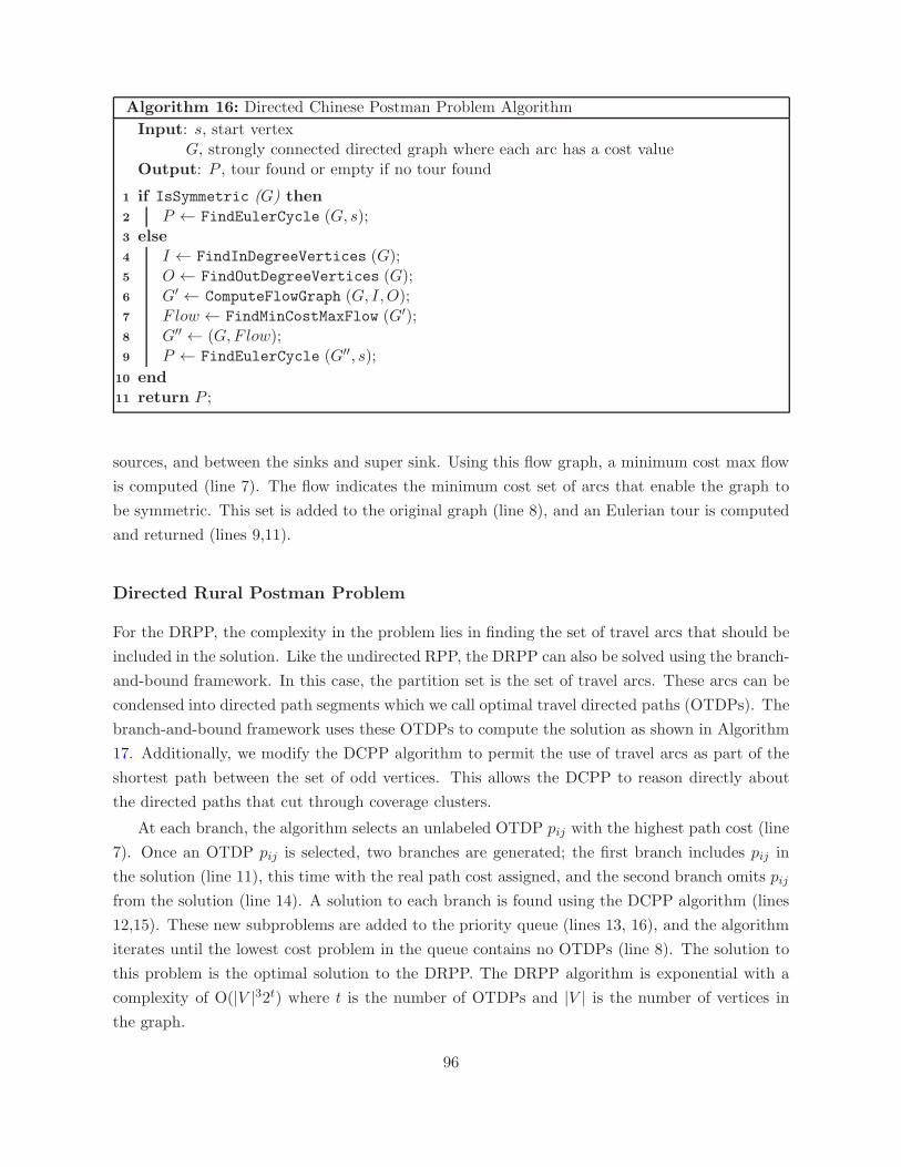
Algorithm 16: Directed Chinese Postman Problem Algorithm

Input: s, start vertexG, strongly connected directed graph where each arc has a cost value

Output: P , tour found or empty if no tour found

1 if IsSymmetric (G) then2 P ← FindEulerCycle (G, s);3 else4 I ← FindInDegreeVertices (G);5 O ← FindOutDegreeVertices (G);6 G′ ← ComputeFlowGraph (G, I,O);7 Flow ← FindMinCostMaxFlow (G′);8 G′′ ← (G,F low);9 P ← FindEulerCycle (G′′, s);

10 end11 return P ;

sources, and between the sinks and super sink. Using this flow graph, a minimum cost max flow

is computed (line 7). The flow indicates the minimum cost set of arcs that enable the graph to

be symmetric. This set is added to the original graph (line 8), and an Eulerian tour is computed

and returned (lines 9,11).

Directed Rural Postman Problem

For the DRPP, the complexity in the problem lies in finding the set of travel arcs that should be

included in the solution. Like the undirected RPP, the DRPP can also be solved using the branch-

and-bound framework. In this case, the partition set is the set of travel arcs. These arcs can be

condensed into directed path segments which we call optimal travel directed paths (OTDPs). The

branch-and-bound framework uses these OTDPs to compute the solution as shown in Algorithm

17. Additionally, we modify the DCPP algorithm to permit the use of travel arcs as part of the

shortest path between the set of odd vertices. This allows the DCPP to reason directly about

the directed paths that cut through coverage clusters.

At each branch, the algorithm selects an unlabeled OTDP pij with the highest path cost (line

7). Once an OTDP pij is selected, two branches are generated; the first branch includes pij in

the solution (line 11), this time with the real path cost assigned, and the second branch omits pij

from the solution (line 14). A solution to each branch is found using the DCPP algorithm (lines

12,15). These new subproblems are added to the priority queue (lines 13, 16), and the algorithm

iterates until the lowest cost problem in the queue contains no OTDPs (line 8). The solution to

this problem is the optimal solution to the DRPP. The DRPP algorithm is exponential with a

complexity of O(|V |32t) where t is the number of OTDPs and |V | is the number of vertices in

the graph.

96

The DCPP algorithm is modified slightly to accommodate the OTDPs. The sources and sinks

of the flow graph are computed on a graph that contains only the coverage arcs. Directed travel

paths made up of OTDPs and travel arcs are added to the flow graph as arcs between the vertices.

In this way, the flow algorithm finds the lowest cost set of arcs to double. Because the optimal

travel paths are now directed, the set of paths in the partition set may be larger since connecting

vertices i to j may consist of two directed paths instead of one undirected path. Additionally,

the path generation algorithm is only used when the graph contains no more OTDPs. Otherwise,

the DCPP algorithm computes the lower bound by adding together the costs of the edges in the

graph with OTDPs having zero cost.

Algorithm 17: Directed Rural Postman Problem Algorithm

Input: s, start vertexG = (C, T ), strongly connected directed graph where each arc has a label and a costvalue. C is the subset of coverage arcs, and T is the subset of travel arcsOTDP , subset of OTDPs

Output: P , tour found or empty if no tour found

1 pq ← [];2 G′ ← [G,OTDP ] where ∀OTDP , cost(pij) = 03 P ← DCPP (s,G′);4 pq.Push ([G′, P ]);5 while HasItems (pq) do6 [G′, P ]← pq.Pop ();7 pij ← FindMaxOTDP (G′);8 if pij == [] then9 return P ;

10 end11 G1 ← IncludeArc (G′, pij);12 P1← DCPP (s,G1);13 pq.Push ([G1, P1]);14 G2 ← RemoveArc (G′, pij);15 P2← DCPP (s,G2);16 pq.Push ([G2, P2]);

17 end18 return [];

Online Replanning

For online replanning, the method proposed by [Thimbleby, 2003] can be used to return paths

that start and end at different vertices. The Farthest Distance heuristic can also be extended

to handle directed graphs. Using these two methods, the DRPP algorithm can effectively replan

when graph changes occur during online traversal.

97

98

Appendix B

Real World Map

The real-world example we used for testing is the road network of an urban neighborhood obtained

from a dataset presented in [Newson and Krumm, 2009]. The network is shown in Figure B.1.

We converted the network into a graph with 764 vertices and 1130 edges.

99

Figure B.1: The road network we used as our real-world example. This network covers an areaof 1.5 miles by 2 miles. The edges and vertices included in our graph are highlighted in blue.

100

Appendix C

Multi-Robot Coverage with

Communication Failure

Communication failures are common in many practical multi-robot coordination tasks where

the robots communicate with one another. We discuss how to handle these failures within the

framework of the parallel branch-and-bound approach. For this problem, we assume that each

robot possesses its own processing unit.

Handling Communication Failures for Parallel Branch-and-bound

Problems

The first step in handling communication breakdowns is to recognize when a breakdown has

occurred. One way to recognize a breakdown is through the use of roll-call and timeout events.

At regular intervals, each robot will announce itself to the other robots as a way of notifying the

rest of the team it is still alive and working – this is the roll-call step. Each robot listens for

the other robots’ announcements. To determine communication or mechanical failures, once a

robot has announced itself a certain number of times, but has not heard from a teammate during

that time, then it deems the teammate to be out of range – this is the timeout step. Using this

communication scheme, robots can keep track of each other in a distributed fashion and detect

disruptions in the communication network.

One major problem that can arise when communication failures occur is the prevention of

environmental change updates to the map. For example, if a particular robot R1 discovers an edge

is blocked during its traversal, under normal circumstances, it would propagate that information

to the rest of the team to update their maps and replan. However, in the event of a communication

breakdown, R1 is unable to share this information with other members of the team. One strategy

to address this problem is for the robots that do receive the new information to replan under

the assumption that a particular subset of the team does not have access to this information.

101

For instance, for a team of four robots, if robots R1 and R2 can communicate and share map

information while being disconnected from robots R3 and R4, then if R1 discovers a change in the

environment, it can notify R2, but not R3 or R4. As a result, R3 and R4 executes their original

plans while R1 and R2 replan using the updated map. Since R1 and R2 do not need to visit the

edges that R3 and R4 are visiting, they modify the updated map labeling the edges that R3 and

R4 are covering as travel edges. This is one way to handle replanning in case of communication

failures.

We conducted a small set of tests to assess the validity of this technique. We evaluated

the quality of the solution by comparing it to the optimal solution obtained in the event of no

communication failure, i.e., robots R3 and R4 also plan using the updated map. For each of the

parallel branch-and-bound calls, the set of robots that are working on the problem and are in

communication uses the auction framework to share subproblems and parts of the search tree.

The tests start with an optimal solution for the initial problem that has been generated by four

robots with perfect communication. Then the communication network breaks down separating

robots R1 and R2 from robots R3 and R4. R1 discovers a change in the graph which corresponds

to a few edges becoming less traversable or having high cost. Next, R1 and R2 replan using

this updated map with the edges they are responsible for labeled as coverage and the remaining

edges labeled as travel. An optimal solution using parallel branch-and-bound with auctions is

computed, and then is divided into two routes using the FHK method. The graphs used for the

testing were the same ones used for the testing done in Chapter 4, section 4.4.2.

Figure C.1 shows the difference between the maximum cost paths generated from replanning

within the group of R1 and R2 (break in communication) and replanning within the team of

four robots (full communication). As the results show, replanning within the team performs

better, but not significantly better than the case with communication loss. Figure C.2 shows

the standard deviation between the paths generated by these two algorithms. While replanning

within the whole team results in lower variance of the path set for most of the graphs, for graph

6, it does significantly worse. This demonstrates that while computing an optimal solution for

the RPP does result in a k-RPP solution with lower bounds, it does not always guarantee paths

with lower variance over a method with looser bounds.

102

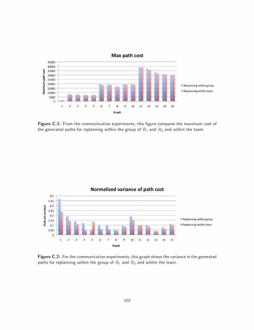
Figure C.1: From the communication experiments, this figure compares the maximum cost ofthe generated paths for replanning within the group of R1 and R2 and within the team.

Figure C.2: For the communication experiments, this graph shows the variance in the generatedpaths for replanning within the group of R1 and R2 and within the team.

103

104

Bibliography

E. U. Acar, H. Choset, A. A. Rizzi, P. N. Atkar, and D. Hull. Morse Decompositions for Coverage

Tasks. The International Journal of Robotics Research, 21(4):331–344, 2002. 3.2.1

E. U. Acar, H. Choset, and J. Y. Lee. Sensor-based Coverage with Extended Range Detectors.

IEEE Transactions on Robotics, 22(1):189–198, Feb. 2006. 3.2.3

N. Agmon, N. Hazon, and G. A. Kaminka. Constructing Spanning Trees for Efficient Multi-Robot

Coverage. In Proceedings of the IEEE International Conference on Robotics and Automation,

2006. 3.2.1

D. Ahr. Contributions to Multiple Postmen Problems. PhD thesis, Heidelberg University, 2004.

3.4.3, 5.1

D. Ahr and G. Reinelt. New Heuristics and Lower Bounds for the Min-Max k-Chinese Postman

Problem. In Algorithms ESA 2002, volume 2461 of Lecture Notes in Computer Science, pages

7–19. 2002. 3.4.3

D. Ahr and G. Reinelt. A Tabu Search Algorithm for the Min-Max k-Chinese Postman Problem.

Computers and Operations Research, 33(12):3403–3422, 2006. 3.4.3

Y. Amit, J. S. B. Mitchell, and E. Packer. Locating Guards for Visibility Coverage of Polygons.

In Workshop on Algorithm Engineering and Experiments. SIAM, 2007. 3.4.2

D. Anguelov, R. Biswas, D. Koller, B. Limketkai, S. Sanner, and S. Thrun. Learning Hierarchi-

cal Object Maps of Non-stationary Environments with Mobile Robots. In Proceedings of the

Conference on Uncertainty in Artificial Intelligence, 2002. 3.1.2

E. M. Arkin, M. A. Bender, E. D. Demaine, S. P. Fekete, J. S. B. Mitchell, and S. Sethia. Optimal

Covering Tours with Turn Costs. In Proceedings of the ACM-SIAM Symposium on Discrete

Algorithms, volume 35, pages 531–566, Philadelphia, PA, USA, 2005. 7.2

A. A. Assad, W. L. Pearn, and B. L. Golden. The Capacitated Chinese Postman Problem: Lower

Bounds and Solvable Cases. American Journal of Mathematical and Management Sciences, 7:

63 – 88, 1987. 3.4.3

T. Bektas. The Multiple Traveling Salesman Problem: An Overview of Formulations and Solution

Procedures. Omega, 34(3):209 – 219, 2006. 3.4.1

105

E. Benavent, A. Carrotta, A. Corbern, J. M. Sanchis, and D. Vigo. Lower Bounds and Heuristics

for the Windy Rural Postman Problem. Technical report, 2003. 3.4.3, 6.6

E. Benavent, A. Corberan, E. Pinana, I. Plana, and J. M. Sanchis. New Heuristic Algorithms

for the Windy Rural Postman Problem. Computers and Operations Research, 32:3111–3128,

December 2005. 3.4.3

E. Benavent, A. Corberan, I. Plana, and J. M. Sanchis. Min-Max k-Vehicles Windy Rural

Postman Problem. Networks, 54(4):216–226, 2009. 3.4.3

R. Biswas, B. Limketkai, S. Sanner, and S. Thrun. Towards Object Mapping in Non-stationary

Environments with Mobile Robots. In Proceedings of the IEEE/RSJ International Conference

on Intelligent Robots and System, volume 1, pages 1014–1019, 2002. 3.1.2

F. Bourgault, A. A. Makarenko, S. B. Williams, B. Grocholsky, and H. F. Durrant-Whyte. Infor-

mation Based Adaptive Robotic Exploration. In Proceedings of the IEEE/RSJ International

Conference on Intelligent Robots and System, volume 1, pages 540–545, 2002. 3.1.2

A. Breitenmoser, M. Schwager, J.-C. Metzger, R. Siegwart, and D. Rus. Voronoi Coverage of

Non-convex Environments with a Group of Networked Robots. In Proceedings of the IEEE

International Conference on Robotics and Automation, pages 4982 –4989, May 2010. 3.2.2

H. Choset. Coverage for Robotics - A Survey of Recent Results. Annals of Mathematics and

Artificial Intelligence, 31:113 – 126, 2001. 3.2.1

H. Choset. Coverage of Known Spaces: The Boustrophedon Cellular Decomposition. Autonomous

Robots, 9:247 – 253, 2000. 3.2.1

H. Choset and J. Burdick. Sensor-based Exploration: The Hierarchical Generalized Voronoi

Graph. The International Journal of Robotics Research, 19(2):96–125, 2000. 3.2.2

H. Choset, S. Walker, K. Eiamsa-Ard, and J. Burdick. Sensor-based Exploration: Incremental

Construction of the Hierarchical Generalized Voronoi Graph. The International Journal of

Robotics Research, 19(2):126–148, 2000. 3.2.2

N. Christofides, E. Benavent, V. Campos, A. Corbern, and E. Mota. An Optimal Method for the

Mixed Postman Problem. In P. Thoft-Christensen, editor, System Modeling and Optimization,

volume 59 of Lecture Notes in Control and Information Sciences, pages 641–649. Springer

Berlin / Heidelberg, 1984. 3.4.3

J. Clossey, G. Laporte, and P. Soriano. Solving Arc Routing Problems with Turn Penalties. The

Journal of the Operational Research Society, 52(4):433–439, 2001. 7.2

A. Corberan, R. Martı, and A. Romero. Heuristics for the Mixed Rural Postman Problem.

Computers and Operations Research, 27:183–203, February 2000. 3.4.3, 6.6

A. Corberan, R. Marti, E. Martinez, and D. Soler. The Rural Postman Problem on Mixed Graphs

with Turn Penalties. Journal of Computers and Operations Research, 29(7):887–903, 2002. 7.2

106

A. Corberan, G. Mejıa, and J. M. Sanchis. New Results on the Mixed General Routing Problem.

Operations Research, 53:363–376, March 2005. 3.4.3

M. B. Dias, R. Zlot, N. Kalra, and A. Stentz. Market-based Multirobot Coordination: A Survey

and Analysis. Proceedings of the IEEE, 94(7):1257 –1270, 2006. 4.4

V. Dimitrijevic and Z. Saric. An Efficient Transformation of the Generalized Traveling Sales-

man Problem into the Traveling Salesman Problem on Digraphs. International Journal of

Information Sciences, 102(1-4):105–110, 1997. 3.4.1

M. Dror, A. Efrat, A. Lubiw, and J. S. B. Mitchell. Touring a Sequence of Polygons. In Proceedings

of the Annual ACM Symposium on the Theory of Computating, pages 473–482. ACM Press,

2003. 3.4.2

K. Easton and J. Burdick. A Coverage Algorithm for Multi-Robot Boundary Inspection. In

Proceedings of the IEEE International Conference on Robotics and Automation, pages 727 –

734, Apr. 2005. 3.4.3, 5.1, 17

J. Edmonds and E. Johnson. Matching, Euler Tours, and the Chinese Postman. Mathematical

Programming, 5(1):88–124, 1973. 3.4.3, 10

J. Edmonds and R. M. Karp. Theoretical Improvements in Algorithmic Efficiency for Network

Flow Problems. Journal of the ACM, 19:248–264, April 1972. 16

A. Efrat and S. Har-Peled. Guarding Galleries and Terrains. Information Processing Letters, 100

(6):238–245, 2006. 3.4.2

H. A. Eiselt, M. Gendreau, and G. Laporte. Arc Routing Problems, Part I: The Chinese Postman

Problem. Operations Research, 43(2):231–242, 1995a. 3.4.3, 3.4.3, A

H. A. Eiselt, M. Gendreau, and G. Laporte. Arc Routing Problems, Part II: The Rural Postman

Problem. Operations Research, 43(3):399–414, 1995b. 3.4.3, 5.2.1, A

P. M. Franca, M. Gendreau, G. Laporte, and F. M. Muller. The m-Traveling Salesman Problem

with Minmax Objective. Transportation Science, 29(3):267–275, 1995. 3.4.1

G. N. Frederickson. Approximation Algorithms for Some Postman Problems. Journal of the

ACM, 26:538–554, July 1979. 3.4.3, 3.4.3, 5.1.1, 3, 6.1.2

G. N. Frederickson, M. S. Hecht, and C. E. Kim. Approximation Algorithms for Some Routing

Problems. Annual IEEE Symposium on the Foundations of Computer Science, 0:216–227,

1976a. 3.4.1

G. N. Frederickson, M. S. Hecht, and C. E. Kim. Approximation Algorithms for Some Routing

Problems. Annual Symposium on Foundations of Computer Science, 7:216 –227, Oct. 1976b.

3.4.3, 5.2, 6.2.1

H. N. Gabow. Implementation of Algorithms for Maximum Matching on Nonbipartite Graphs.

PhD thesis, Stanford, CA, USA, 1974. 10

107

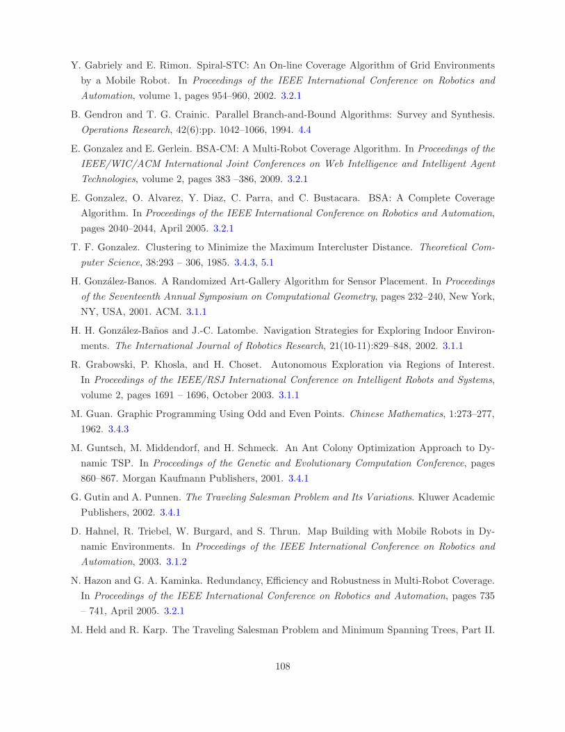
Y. Gabriely and E. Rimon. Spiral-STC: An On-line Coverage Algorithm of Grid Environments

by a Mobile Robot. In Proceedings of the IEEE International Conference on Robotics and

Automation, volume 1, pages 954–960, 2002. 3.2.1

B. Gendron and T. G. Crainic. Parallel Branch-and-Bound Algorithms: Survey and Synthesis.

Operations Research, 42(6):pp. 1042–1066, 1994. 4.4

E. Gonzalez and E. Gerlein. BSA-CM: A Multi-Robot Coverage Algorithm. In Proceedings of the

IEEE/WIC/ACM International Joint Conferences on Web Intelligence and Intelligent Agent

Technologies, volume 2, pages 383 –386, 2009. 3.2.1

E. Gonzalez, O. Alvarez, Y. Diaz, C. Parra, and C. Bustacara. BSA: A Complete Coverage

Algorithm. In Proceedings of the IEEE International Conference on Robotics and Automation,

pages 2040–2044, April 2005. 3.2.1

T. F. Gonzalez. Clustering to Minimize the Maximum Intercluster Distance. Theoretical Com-

puter Science, 38:293 – 306, 1985. 3.4.3, 5.1

H. Gonzalez-Banos. A Randomized Art-Gallery Algorithm for Sensor Placement. In Proceedings

of the Seventeenth Annual Symposium on Computational Geometry, pages 232–240, New York,

NY, USA, 2001. ACM. 3.1.1

H. H. Gonzalez-Banos and J.-C. Latombe. Navigation Strategies for Exploring Indoor Environ-

ments. The International Journal of Robotics Research, 21(10-11):829–848, 2002. 3.1.1

R. Grabowski, P. Khosla, and H. Choset. Autonomous Exploration via Regions of Interest.

In Proceedings of the IEEE/RSJ International Conference on Intelligent Robots and Systems,

volume 2, pages 1691 – 1696, October 2003. 3.1.1

M. Guan. Graphic Programming Using Odd and Even Points. Chinese Mathematics, 1:273–277,

1962. 3.4.3

M. Guntsch, M. Middendorf, and H. Schmeck. An Ant Colony Optimization Approach to Dy-

namic TSP. In Proceedings of the Genetic and Evolutionary Computation Conference, pages

860–867. Morgan Kaufmann Publishers, 2001. 3.4.1

G. Gutin and A. Punnen. The Traveling Salesman Problem and Its Variations. Kluwer Academic

Publishers, 2002. 3.4.1

D. Hahnel, R. Triebel, W. Burgard, and S. Thrun. Map Building with Mobile Robots in Dy-

namic Environments. In Proceedings of the IEEE International Conference on Robotics and

Automation, 2003. 3.1.2

N. Hazon and G. A. Kaminka. Redundancy, Efficiency and Robustness in Multi-Robot Coverage.

In Proceedings of the IEEE International Conference on Robotics and Automation, pages 735

– 741, April 2005. 3.2.1

M. Held and R. Karp. The Traveling Salesman Problem and Minimum Spanning Trees, Part II.

108

Mathematical Programming, 6:62–88, 1971. 3.4.1

D. S. Johnson and L. A. Mcgeoch. The Traveling Salesman Problem: A Case Study. In Local

Search in Combinatorial Optimization. Wiley and Sons, 1997. 3.4.1

E. G. Jones. Multi-Robot Coordination in Domains with Intra-Path Constraints. PhD thesis,

Robotics Institute, Carnegie Mellon University, Pittsburgh, PA, August 2009. 4.4

S. Koenig and M. Likhachev. Improved Fast Replanning for Robot Navigation in Unknown

Terrain. In Proceedings of the IEEE International Conference on Robotics and Automation,

volume 1, pages 968–975, 2002. 9

T. Kollar and N. Roy. Trajectory Optimization Using Reinforcement Learning for Map Explo-

ration. The International Journal of Robotics Research, 27(2):175–196, 2008. 3.1.2

B. Korte and J. Vygen. Combinatorial Optimization: Theory and Algorithms. Springer, Germany,

3rd edition, 2006. 3.4.1

J. B. Kruskal. On the Shortest Spanning Subtree of a Graph and the Traveling Salesman Problem.

In Proceedings of the American Mathematical Society, volume 7, page 4850, 1956. 12

G. Laporte. Modeling and Solving Several Classes of Arc Routing Problems as Traveling Salesman

Problems. Computers and Operations Research, 24(11):1057–1061, 1997. 3.4.3, 3.4.3

G. Laporte, A. Asef-Vaziri, and C. Sriskandarajah. Some Applications of the Generalized Trav-

eling Salesman Problem. The Journal of the Operational Research Society, 47(12):1461–1467,

1996. 3.4.1

D. Latimer, S. Srinivasa, V. Lee-Shue, S. Sonne, H. Choset, and A. Hurst. Towards Sensor Based

Coverage with Robot Teams. In Proceedings of the IEEE International Conference on Robotics

and Automation, volume 1, pages 961 – 967, 2002. 3.2.1

D. Lee and A. Lin. Computational Complexity of Art Gallery Problems. IEEE Transactions on

Information Theory, 32(2):276–282, Mar 1986. 3.4.2

S. Lin and B. W. Kernighan. An Effective Heuristic Algorithm for the Traveling-Salesman Prob-

lem. Operations Research, 21(2):498–516, 1973. 3.4.1

Y. Liu, S. Zhu, B. Jin, S. Feng, and H. Gong. Sensory Navigation of Autonomous Cleaning Robots.

Fifth World Congress on Intelligent Control and Automation, 6:4793–4796, June 2004. 3.2.1

V. J. Lumelsky, S. Mukhopadhyay, and K. Sun. Dynamic Path Planning in Sensor-based Terrain

Acquisition. IEEE Transactions on Robotics and Automation, 6(4):462–472, Aug 1990. 3.2.1

J. B. MacQueen. Some Methods for Classification and Analysis of Multivariate Observations. In

Proceedings of the Fifth Berkeley Symposium on Mathematical Statistics and Probability, pages

281–297, 1967. 5.1.1, 6.2.2

R. Mannadiar and I. Rekleitis. Optimal Coverage of a Known Arbitrary Environment. In Pro-

ceedings of the IEEE International Conference on Robotics and Automation, pages 5525 –5530,

109

May 2010. 3.4.3

J. Maver and R. Bajcsy. Occlusions as a Guide for Planning the Next View. IEEE Transactions

on Pattern Analysis and Machine Intelligence, 15(5):417–433, 1993. 3.1.1

E. Minieka. Optimization Algorithms for Networks and Graphs. M. Dekker, New York, 1978. 10

L. M. Moreira, J. F. Oliveira, A. M. Gomes, and J. S. Ferreira. Heuristics for a Dynamic Rural

Postman Problem. Computers and Operations Research, 34(11):3281–3294, 2007. 3.4.3

A. R. Mosteo and L. Montano. Comparative Experiments on Optimization Criteria and Algo-

rithms for Auction Based Multi-Robot Task Allocation. In Proceedings of the IEEE Interna-

tional Conference on Robotics and Automation, pages 3345 –3350, April 2007. 5

P. Newson and J. Krumm. Seattle Road Network Data. http://research.microsoft.com/en-

us/um/people/jckrumm/MapMatchingData/data.htm, 2009. B

Y. Nobert and J.-C. Picard. An Optimal Algorithm for the Mixed Chinese Postman Problem.

Networks, 27(2):95–108, 1996. 3.4.3

J. S. Oh, Y. H. Choi, J. B. Park, and Y.F. Zheng. Complete Coverage Navigation of Cleaning

Robots using Triangular-Cell-based Map. IEEE Transactions on Industrial Electronics, 51(3):

718–726, 2004. 3.2.1

B. Raghavachari and J. Veerasamy. Approximation Algorithms for Mixed Postman Problem.

SIAM Journal of Discrete Mathematics, 12, 1998. 3.4.3, 6.1.2

I. M. Rekleitis, G. Dudek, and E. E. Milios. Multi-Robot Collaboration for Robust Exploration.

In Proceedings of the IEEE International Conference on Robotics and Automation, volume 4,

pages 3164 –3169, 2000. 3.1.1

E. Rothberg. Implementation of H. Gabow’s Weighted Matching Algorithm.

ftp://dimacs.rutgers.edu/pub/netflow/matching/weighted/, 1992. 10

S. Safra and O. Schwartz. On the Complexity of Approximating TSP with Neighborhoods and

Related Problems. Computational Complexity, 14(4):281–307, 2006. 3.4.1

G. Schmidt and C. Hofner. An Advanced Planning and Navigation Approach for Autonomous

Cleaning Robot Operations. In Proceedings of the IEEE/RSJ International Conference on

Intelligent Robots and Systems, volume 2, pages 1230–1235, 1998. 3.2.1

R. Simmons, D. Apfelbaum, W. Burgard, D. Fox, M. Moors, S. Thrun, and H. Younes. Co-

ordination for Multi-Robot Exploration and Mapping. In Proceedings of the AAAI National

Conference on Artificial Intelligence, Austin, TX, 2000. AAAI. 3.1.1

C. G. Sorensen, T. Bak, and R. N. Jorgensen. Mission Planner for Agricultural Robotics. Agri-

cultural Engineering International, 2004. 3.4.3

C. Stachniss and W. Burgard. Exploring Unknown Environments with Mobile Robots Using

Coverage Maps. In Proceedings of the International Conference on Artificial Intelligence, 2003.

110

3.1.1

H. Surmann, A. Nuchter, and J. Hertzberg. An Autonomous Mobile Robot with a 3D Laser

Range Finder for 3D Exploration and Digitalization of Indoor Environments. Robotics and

Autonomous Systems, 45(3-4):181–198, 2003. 3.1.1

X. Tan. A Linear-time 2-Approximation Algorithm for the Watchman Route Problem for Simple

Polygons. Theoretical Computer Science, 384(1):92 – 103, 2007. 3.4.2

G. S. Tewolde and W. Sheng. Robot Path Integration in Manufacturing Processes: Genetic

Algorithm Versus Ant Colony Optimization. In Proceedings of the IEEE Transactions on

Systems, Man and Cybernetics, Part A: Systems and Humans, volume 38, pages 278 –287,

March 2008. 3.4.3

H. Thimbleby. The Directed Chinese Postman Problem. Journal of Software Practice and Expe-

rience, 33:2003, 2003. 6.2.3, 18

K. Williams and J. Burdick. Multi-Robot Boundary Coverage with Plan Revision. In Proceedings

of the IEEE International Conference on Robotics and Automation, pages 1716 –1723, May.

2006. 3.4.3, 5.1, 5.1.2

M. Grotscheland Z. Win. A Cutting Plane Algorithm for the Windy Postman Problem. Mathe-

matical Programming, 55:339–358, June 1992. 3.4.3

L. Xu and A. Stentz. Blended Local Planning for Generating Safe and Feasible Paths. In

Proceedings of the IEEE/RSJ International Conference on Intelligent Robots and Systems,

pages 709–716, Sept. 2008. 7.2

B. Yamauchi. A Frontier-based Approach for Autonomous Exploration. In Proceedings of the

IEEE International Symposium on Computational Intelligence in Robotics and Automation,

pages 146–151, Jul 1997. 3.1.1

B. Yamauchi. Frontier-based Exploration Using Multiple Robots. In Proceedings of the Second

International Conference on Autonomous Agents, AGENTS ’98, pages 47–53, New York, NY,

USA, 1998. ACM. 3.1.1

A. Zelinsky, R. A. Jarvis, J. C. Byrne, and S. Yuta. Planning Paths of Complete Coverage of an

Unstructured Environment by a Mobile Robot. In Proceedings of International Conference on

Advanced Robotics, pages 533–538, 1993. 3.2.1

L. Zhang. Polynomial Algorithms for the k-Chinese Postman Problem. In IFIP World Computer

Congress on Algorithms, Software, Architecture - Information Processing, pages 430–435, 1992.

3.4.3

X. Zheng, S. Jain, S. Koenig, and D. Kempe. Multi-Robot Forest Coverage. In Proceedings of

the IEEE International Conference on Intelligent Robots and Systems, pages 3852 – 3857, Aug.

2005. 3.2.1

111

A. Zhou, L. Kang, and Z. Yan. Solving Dynamic TSP with Evolutionary Approach in Real Time.

The Congress on Evolutionary Computation, 2:951–957, Dec. 2003. 3.4.1

R. M. Zlot, A. Stentz, M. B. Dias, and S. Thayer. Multi-Robot Exploration Controlled by

a Market Economy. In Proceedings of the IEEE International Conference on Robotics and

Automation, pages 3016 – 3023, May 2002. 3.1.1, 4.4

112