Graph-Based Navigation Strategies for Heterogeneous Spatial Data Sets

Graph-based Navigation Strategies forHeterogeneous Spatial Data Sets

Andrea Rodrıguez1 and Francisco Godoy2

1 Department of Computer Science, University of ConcepcionEdmundo Larenas 215, 4070409 Concepcion, Chile

[email protected] Center for Oceanographic Research in the Eastern South-Pacific

FONDAP-COPAS, University of ConcepcionP.O. Box 160-C, Concepcion, Chile

[email protected]

Abstract. Querying heterogeneous spatial databases involves not onlycharacterizing and comparing the information content of several databases,but also navigating or accessing the data sets with the query answer.This work proposes a formalism that relates the information content ofdata sets by three basic types of correspondence relations: data equiv-alence, difference of data omission, and difference of data commission.These correspondence relations define the information space over whicha navigation process is carried out. Based on a complete or an incom-plete information space, this work proposes strategies that optimize theretrieval process of information coming from different databases. The re-sults of this study show the advantages of defining the information spaceto select and access databases. In particular, strategies that estimate theinformation contribution of data sets based on correspondence relationsoutperform a strategy that considers a random list or a list of data setssorted by size.

1 Introduction

In presence of syntactic, schematic, and semantic differences [15], accessing dis-tributed databases requires an important effort to compare user queries withdata stored in diverse databases. Most research in this area has focused on es-tablishing the relationship among databases; that is, similarity, difference, andequivalence between database schemas [8] [7] [12] [17] [9]. A subsequent, but notless important, issue in querying and accessing heterogeneous databases dealswith the way users navigate among data sets that contain the query answer.Users are typically presented with only a ranked list of databases that totallyor partially satisfy their requests and then, they have to decide which of thesedatabases they will access.

This work considers the process of accessing different databases that containdesired data as a problem of information navigation. For example, consider auser who wants to retrieve data of utility networks in a given urban area. These

data may be obtained from different databases, each of them containing partialdata of utility networks. The query to each database may result in differentdata sets (i.e., sets of tuples in relational databases), and users have to decidewhat data sets and in which sequence should be accessed. We claim that is notonly important to know what databases contain the desired data, but to providewith strategies to organize the results of the query so that an efficient retrievalprocess is accomplished. In this context, efficiency refers to getting all or mostinformation (i.e., new data) with the access to few databases.

The contribution of this work relates to the navigation in an informationspace composed of heterogeneous spatial data sets. This can be done afterdatabase schemas or metadata have been compared and databases that containthe desired type of data have been detected. This work proposes a formalism thatallows one to relate spatial databases in terms of the equivalences and differencesbetween their data sets.

We define an information space by characterizing the correspondences be-tween data sets with three basic categories: data equivalence, difference of dataomission, and difference of data commission. Using these categories in a graph-base representation, this work describes strategies that optimize the navigationof data sets with the query results. The objective of this optimization is to re-trieve data that contribute to the answer, minimizing duplications while increas-ing the data retrieved. The work concentrates on spatial objects represented byregions. At an abstract level, the same approach may be useful in other domainsof information.

The structure of the paper is as follows. Section 2 gives a brief review ofrelated work. Section 3 describes the modeling of the information space with thecorrespondence relations between data sets and the graph-based representation.Section 4 presents the different strategies for information navigation, and Sec-tion 5 shows the implementation of the strategies. Final conclusions and futureresearch directions are given in Section 6.

2 Related Work

In the area of information systems, the concept of information navigation hasbeen associated with the visualization of retrieval results. In a retrieval processwith heterogeneous data collections that totally and partially satisfied a userquery, the problem becomes to select and browse the query results. The generalidea for solving this problem is to use overviews of the information that mayguide users in the retrieval process [2]. We consider the process of selecting andbrowsing documents as a process of information navigation, where two importantapproaches are:

– Category hierarchies. This approach assigns metadata to data sets based ontheir categories, which are then organized into a hierarchy. The problem withthis strategy is that one could often need to look at a large collection of tagsand, when the category has been found, search within the category. Examplesof this type of approach are the computer classification system of the ACM

[1], which has developed a hierarchy of 1200 categories or the the popularsearch site Yahoo [19], which organized documents in many categories.

– Clustering techniques. There are several cluster-based solutions for helpingusers in searching and navigating data sets. They attempt to display overviewinformation derived from the metadata or the extraction of common featuresin a collection. Then, clusters group data sets based on the similarity to oneanother. An early contribution is the paradigm Scatter/Gatter [3], whereusers are provided with a summary of the documents that have been clus-tered. More recent works have also considered dynamic clusters [20] andclustering and summary of query results for information navigation [14]. Anexample of such approaches is the web site VIVISIMO [16], which dynami-cally organizes the query results by topics.

A second perspective of information navigation relates to the process of ac-cessing heterogeneous data sources. In this context, the navigation is carriedout over a semantic structure, called information space, that connects differentsources [13]. This work concerns the second perspective of a navigation process.It defines a structure upon which different strategies for selecting the path inthe navigation process can be taken.

3 The Information Space

The information space describes the content relations between data sets. Theserelations are basic correspondence categories upon which a graph representationis defined to be used in the navigation process.

3.1 Types of correspondences between data sets

Three types of basic correspondence relations between data sets are: equivalence,difference of commission, and difference of omission. The distinction betweendifference of commission and difference of omission resembles the notions oferror of commission and error of omission, respectively, associated with typesof inaccuracy in an ontology of imperfection for information integration [18]. Insuch ontology, inaccuracy is the lack of correlation with the actual state of affair.Our notions of difference of commission and difference of omission, however,do not relate to errors. Commission and omission are here converse conceptsrelated to the presence or absence of data, respectively. Since this work assumesno further information about the origin of data, all data sets are considered toequally contribute to the integration or retrieval of information. Thus, solvingconflicting geometric representations (e.g., two different geometries for a sameobject) is a process carried out after all data are retrieved.

A definition of the correspondence relations follows.

– Equivalence. Considering the same thematic layer, two objects are said to beequivalent if they occupied the same space or have the same representativeset of coordinates. We relax the definition of equivalence for not totally

equivalent objects by considering that two objects from different databasesand a same thematic layer are represented by equivalent and different regions.The equivalent regions are the intersection of the geometric representations ofobjects, whereas the different regions are the non intersecting representationsof objects. This difference between objects is further classified into differenceof commission and difference of omission.Let x, y, z be regions belonging to objects from different data sets, then theequivalence relation between x and y (x ≡ y) satisfies the following basicproperties:

∀ x, y [x ≡ y → y ≡ x] symmetry (1)∀ x, y, z [(x ≡ y ∧ y ≡ z) → x ≡ z] transitivity (2)

We define an Equivalent Operator between two data sets A and B (E(A,B))to be the equivalent regions between the data sets. The total area of theseequivalent regions will be expressed by |E(A,B)|.

– Difference of commission. The difference of omission between two data setsA and B (C(A,B)) corresponds to the regions that are in A and not in B.

– Difference of omission. As the converse relation of C(A,B), the difference ofomission between data sets A and B (O(A,B)) corresponds to the regionsthat are in B and not in A.

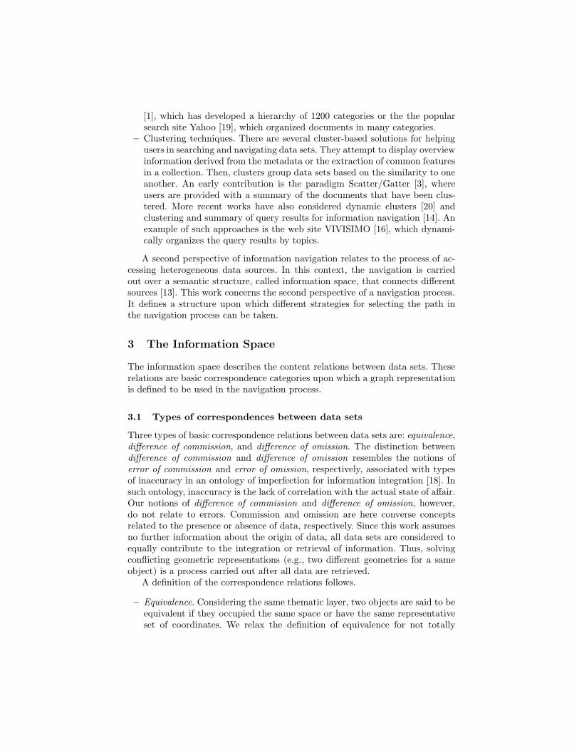
Figure 1 presents the basic cases of the three types of correspondence betweendata sets A and B when considering the same spatial window ω. In this case,features a and c are equivalent in both data sets, feature b is in data set A butnot in B; that is, there is a difference of commission of feature b between datasets A and B, and a difference of omission of feature b between data sets B andA. Likewise, d is a feature in data set B and not in data set A.

a b

c

a

dc

ωω

A B

Fig. 1. Example of equivalences and differences between data sets

In the case of partial equivalence and matching of composite objects betweentwo data sets A, B, the operators |E(A,B)|, |C(A,B)| and |O(A,B)| define thepercentages of areas that are equivalent and different, without indicating how

many objects are really equivalent or different. A further study could analyzewhen an object is equivalent or not, a problem that has been addressed in studiesof data integration [18] [6] and consistency at multiple representations [5] [10][4].

Let a and b be the total areas of objects in data sets A and B, respectively,the correspondence operators satisfy the following properties:

a = |E(A,A)| (3)a = |E(A,B)| + |C(A,B)| (4)a = |E(A,B)| + |O(B,A)| (5)b = (a − |O(B,A)|) + |O(A,B)| (6)

3.2 Graph-based representation of the information space

The set of data sets with their correspondence relations can be seen as a directedand labeled graph, with nodes being data sets and edges being the correspon-dence categories between data sets. The graph can be simplified by using onlyone directed edge between nodes, since the inverse directed edge can be deter-mined by the converse properties |C(A,B)| = |O(B,A)|.

For n data sets, a complete graph is of order O(n2). Under incomplete infor-mation, the composition of correspondence relations allows one to constrain thepossible values of unknown information. Thus, a composition of correspondencerelations between data sets A and B and between B and C indicates possiblevalues for the correspondence relations between A and C.

Proposition 1. Given three different data sets A, B, and C, with total areasof objects a, b, and c, respectively, and where known information are the resultsof the equivalent operator between A and B (E(A,B)) and between B and C(E(B,C)), the value of |E(A,C)| has lower and upper bounds given by

∀A,B,C[max(0, |E(A,B)| + |E(B,C)| − b) ≤ |E(A,C)| ≤ min(a, c)] (7)

Proof. A lower bound of equivalent areas between data sets A and C isdetermined by the minimum area of regions that are in common between regionsin E(A,B) and E(B,C). These regions must be also in the equivalent regionsbetween A and C by the transitivity property of equivalence (Equation 2).The minimum area can be obtained from the maximum area of regions that aredifferent between the equivalent regions E(A,B) and E(B,C). In order to have aregion in E(A,B) that is not in E(B,C), the equivalent region in E(A,B) mustbe in C(B,C). Thus, we cannot have more regions that are different betweenE(A,B) and C(B,C). Once |C(B,C)| is less than |E(A,B)|, the lower boundof |E(A,C)| is equal to |E(A,B)| − |C(B,C)|. Once |C(B,C)| is larger than|E(A,B)|, the lower bound of |E(A,C)| is equal to zero, since it assumes thatall equivalent regions between A and B are also in the set of regions that are inB and not in C.

An upper bound of the area of equivalent regions between data sets A andC is given by the minimum area of the space used by objects in each data set,since one cannot have an area of equivalent regions larger than the total area ofobjects in the data sets.

Corollary 1. Given that |C(A,C)| = a−|E(A,C)| and |O(A,C)| = c−|E(A,C)|,then

∀A,B,C[a − min(a, c) ≤ |C(A,C)| ≤ a − max(0, |E(A,B)| − |C(B,C)|)] (8)∀A,B,C[c − min(a, c) ≤ |O(A,C)| ≤ c − max(0, |E(A,B)| − |C(B,C)|)] (9)

4 Information Navigation

The navigation strategies proposed in this paper aim at retrieving all data witha minimum effort or cost. Effort or cost in this case are considered to be the totalamount of retrieved data, measured as the total area of objects retrieved. In suchretrieval process, duplication may occur and the idea is to obtain all data, whileaccessing the minimum number of databases or accessing databases in a sequencethat obtains most data as quick as possible. For all data we mean all differentregions, since these regions are the real information contribution of data sets. Ifone of the data sets retrieved from a database contains all regions (objects) in adesired geographic window, the system should just access this database to obtaina complete answer. In an imperfect world, however, databases are incomplete. Insuch cases, to obtain a complete answer means to access more than one database,but hopefully, not all of them.

4.1 Navigation Strategies

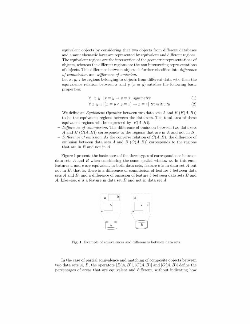
There are different strategies retrieving all data from an information space. To il-lustrate the different alternatives, consider a simple case of four data sets (comingfrom different databases) (Figure 2), whose correspondence relations are codifiedby the triple (|O()|, E()|, |C()|) as labels of the directed graph, and where the to-tal area of objects in each data set is codified by the value in each correspondingnode.

Common to all strategies is that they favor data sets with large objects’geometries. It is not the number of objects, but the objects that occupy morespace what will guide the navigation strategy.

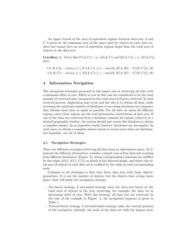
– Size-based strategy. A size-based strategy sorts the data sets based on thetotal area of objects in the sets, retrieving, for example, the data set indecreasing order of area. With this strategy, all data sets are retrieved. Inthe case of the example in Figure 2, the navigation sequence is given inTable 1.

– Forward-based strategy. A forward-based strategy takes the current positionof the navigation (initially, the node of the data set with the largest area)

10

A

20

B

12C

15D

(2,8,12)

(6,4,11)

(8,7,5)

(5,7,3)

(7,5,15)

(8,7,13)

Fig. 2. Complete graph with four data sets

Data Set Total area Sequence order

A 10 4B 20 1C 12 3D 15 2

Table 1. An example of navigation with the size-based strategy

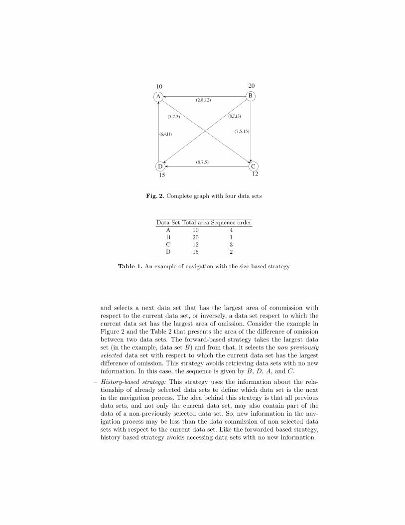
and selects a next data set that has the largest area of commission withrespect to the current data set, or inversely, a data set respect to which thecurrent data set has the largest area of omission. Consider the example inFigure 2 and the Table 2 that presents the area of the difference of omissionbetween two data sets. The forward-based strategy takes the largest dataset (in the example, data set B) and from that, it selects the non previouslyselected data set with respect to which the current data set has the largestdifference of omission. This strategy avoids retrieving data sets with no newinformation. In this case, the sequence is given by B, D, A, and C.

– History-based strategy: This strategy uses the information about the rela-tionship of already selected data sets to define which data set is the nextin the navigation process. The idea behind this strategy is that all previousdata sets, and not only the current data set, may also contain part of thedata of a non-previously selected data set. So, new information in the nav-igation process may be less than the data commission of non-selected datasets with respect to the current data set. Like the forwarded-based strategy,history-based strategy avoids accessing data sets with no new information.

O() A B C D

A 0 12 5 11B 2 0 7 8C 3 15 0 8D 6 13 5 0

Table 2. An example of navigation with the forward-based strategy

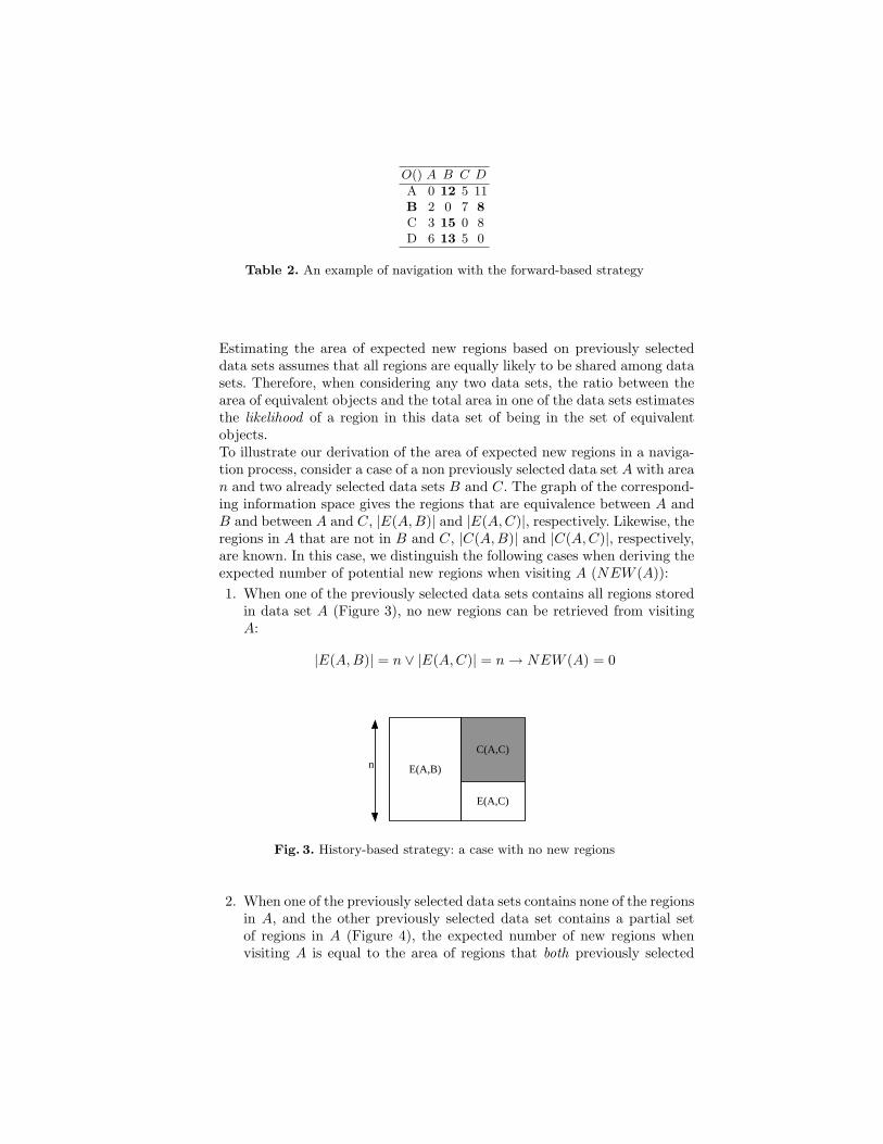
Estimating the area of expected new regions based on previously selecteddata sets assumes that all regions are equally likely to be shared among datasets. Therefore, when considering any two data sets, the ratio between thearea of equivalent objects and the total area in one of the data sets estimatesthe likelihood of a region in this data set of being in the set of equivalentobjects.To illustrate our derivation of the area of expected new regions in a naviga-tion process, consider a case of a non previously selected data set A with arean and two already selected data sets B and C. The graph of the correspond-ing information space gives the regions that are equivalence between A andB and between A and C, |E(A,B)| and |E(A,C)|, respectively. Likewise, theregions in A that are not in B and C, |C(A,B)| and |C(A,C)|, respectively,are known. In this case, we distinguish the following cases when deriving theexpected number of potential new regions when visiting A (NEW (A)):1. When one of the previously selected data sets contains all regions stored

in data set A (Figure 3), no new regions can be retrieved from visitingA:

|E(A,B)| = n ∨ |E(A,C)| = n → NEW (A) = 0

E(A,B)

C(A,C)

E(A,C)

n

Fig. 3. History-based strategy: a case with no new regions

2. When one of the previously selected data sets contains none of the regionsin A, and the other previously selected data set contains a partial setof regions in A (Figure 4), the expected number of new regions whenvisiting A is equal to the area of regions that both previously selected

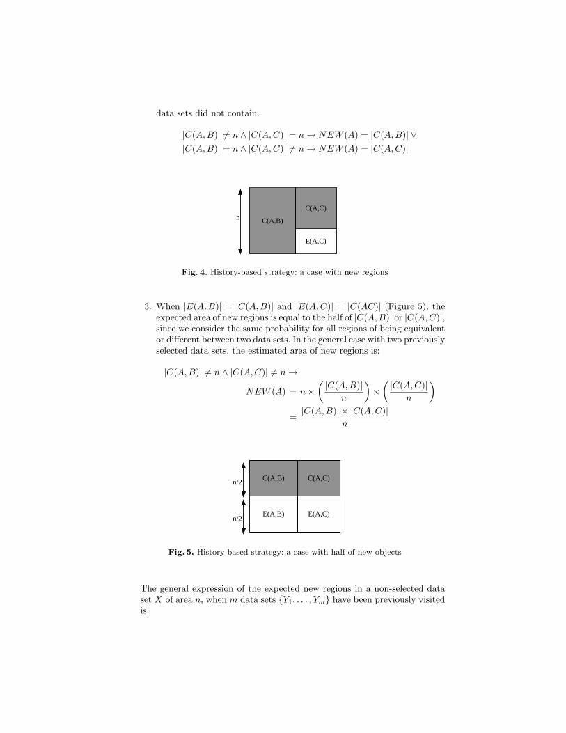
data sets did not contain.

|C(A,B)| �= n ∧ |C(A,C)| = n → NEW (A) = |C(A,B)| ∨|C(A,B)| = n ∧ |C(A,C)| �= n → NEW (A) = |C(A,C)|

C(A,B)

C(A,C)

E(A,C)

n

Fig. 4. History-based strategy: a case with new regions

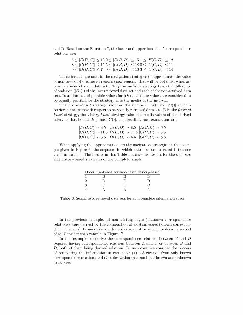
3. When |E(A,B)| = |C(A,B)| and |E(A,C)| = |C(AC)| (Figure 5), theexpected area of new regions is equal to the half of |C(A,B)| or |C(A,C)|,since we consider the same probability for all regions of being equivalentor different between two data sets. In the general case with two previouslyselected data sets, the estimated area of new regions is:

|C(A,B)| �= n ∧ |C(A,C)| �= n →NEW (A) = n ×

( |C(A,B)|n

)×

( |C(A,C)|n

)

=|C(A,B)| × |C(A,C)|

n

C(A,B) C(A,C)n/2

E(A,B) E(A,C)n/2

Fig. 5. History-based strategy: a case with half of new objects

The general expression of the expected new regions in a non-selected dataset X of area n, when m data sets {Y1, . . . , Ym} have been previously visitedis:

NEW (X) =

∏i �=j |C(Yi, Yj)|

nm−1(10)

In the example of Figure 2, this strategy takes the data set with the largestarea and continues accessing the non-selected data sets in the following se-quence: B, D, C and A.

4.2 Incomplete Information Space

Since the cost of constructing a complete information space may be very high,this section analyzes the strategies in presence of an incomplete representationof the information space. In this analysis, the total area of objects per data set isknown, and the data equivalence, difference of data commission, and difference ofdata omission may be unknown. The focus of the analysis is on the equivalence,since knowing the data equivalence between data sets and the total area perdata set allows us to quantify the differences between data sets.

The size-based strategy is not affected by the incomplete information space.The last two strategies, forward- and history-based strategies, however, needsome derivation or approximation. Useful to this approximation are the lowerand upper bounds defined by composition of correspondence relations describedin Section 2.2. Such an approximation requires a connected information space(connected graph); that is, there exists at least one path between any two nodesin the graph representation. Consider for example the connected and incompleteinformation space in Figure 6.

10

A

20

B

12C

15D

(2,8,12)

(6,4,11)

(5,7,3)

Fig. 6. Example 1: Incomplete and connected information space

In the information space of Figure 6, three edges of correspondence relationsare missing: edge between B and C, edge between B and D, and edge between C

and D. Based on the Equation 7, the lower and upper bounds of correspondencerelations are:

5 ≤ |E(B,C)| ≤ 12 2 ≤ |E(B,D)| ≤ 15 1 ≤ |E(C,D)| ≤ 128 ≤ |C(B,C)| ≤ 15 5 ≤ |C(B,D)| ≤ 18 0 ≤ |C(C,D)| ≤ 110 ≤ |O(B,C)| ≤ 7 0 ≤ |O(B,D)| ≤ 13 3 ≤ |O(C,D)| ≤ 14

These bounds are used in the navigation strategies to approximate the valueof non-previously retrieved regions (new regions) that will be obtained when ac-cessing a non-retrieved data set. The forward-based strategy takes the differenceof omission (|O()|) of the last retrieved data set and each of the non-retrived datasets. In an interval of possible values for |O()|, all these values are considered tobe equally possible, so the strategy uses the media of the interval.

The history-based strategy requires the numbers |E()| and |C()| of non-retrieved data sets with respect to previously retrieved data sets. Like the forward-based strategy, the history-based strategy takes the media values of the derivedintervals that bound |E()| and |C()|. The resulting approximations are:

|E(B,C)| � 8.5 |E(B,D)| � 8.5 |E(C,D)| � 6.5|C(B,C)| � 11.5 |C(B,D)| � 11.5 |C(C,D)| � 5.5|O(B,C)| � 3.5 |O(B,D)| � 6.5 |O(C,D)| � 8.5

When applying the approximations to the navigation strategies in the exam-ple given in Figure 6, the sequence in which data sets are accessed is the onegiven in Table 3. The results in this Table matches the results for the size-baseand history-based strategies of the complete graph.

Order Size-based Forward-based History-based

1 B B B2 D D D3 C C C4 A A A

Table 3. Sequence of retrieved data sets for an incomplete information space

In the previous example, all non-existing edges (unknown correspondencerelations) were derived by the composition of existing edges (known correspon-dence relations). In same cases, a derived edge must be needed to derive a secondedge. Consider the example in Figure 7.

In this example, to derive the correspondence relations between C and Drequires having correspondence relations between A and C or between B andD, both of them being derived relations. In such case, we consider the processof completing the information in two steps: (1) a derivation from only knowncorrespondence relations and (2) a derivation that combines known and unknowncategories.

10

A

20

B

12C

15D

(2,8,12)

(6,4,11)(7,5,15)

Fig. 7. Example 2: Incomplete and connected information space

An algebraic analysis of using a derived correspondence relations to derivea new correspondence relations follows. Constants are the total areas per dataset or the known correspondence relations. Consider the example in Figure 7,the constants a, b, c are the areas in data sets A, B, and C, respectively. Thederivation of |E(A,C)| follows the Equation 11.

max(0, |E(A,B)| − (b − |E(B,C)|) ≤ |E(A,C)| ≤ min(a, c) (11)

If d ≤ |E(A,B)| ≤ e, where d and e are previously derived lower and upperbounds, then

max(0, d − (b − |E(B,C)|) ≤ |E(A,C)| ≤ min(a, c)

includes all possible values of |E(A,C)|, since the effect of the upper bound of|E(A,B)| is already considered within the interval between the lower bound of|E(A,B)| and the upper bound of |E(A,C)|. Likewise, if d ≤ |E(B,C)| ≤ e,then

max(0, |E(A,B)| − (b − d) ≤ |E(A,C)| ≤ min(a, c)

includes all posssible values.When deriving the correspondence relations, if there exist more than one

composition path between data sets, it is the intersection of all intervals derivedfrom composition paths of length 2 between data sets what defines the intervalof a correspondence relation. Such intersection comes from the definition of pathconsistency of logical consistency in a graph [11].

In the intersection of these intervals, upper bounds of different compositionpaths between two data sets are the same, since these intervals are bounded by

the minimum of total objects between data sets. For lower bound, the intersectionis equivalent to the maximum of lower bounds. For example, the derivation of|E(C,D)| in Figure 7 can be done by using |E(C,B)| and |E(B,D)| or by using|E(C,A)| and |E(A,D)|. Thus, it is the intersection of both results what defines|E(C,D)|. The derived intervals of the example in Figure 7 are:

0 ≤ |E(A,C)| ≤ 10 2 ≤ |E(B,D)| ≤ 15 0 ≤ |E(C,D)| ≤ 120 ≤ |C(A,C)| ≤ 10 5 ≤ |C(B,D)| ≤ 18 0 ≤ |C(C,D)| ≤ 122 ≤ |O(A,C)| ≤ 12 0 ≤ |O(B,D)| ≤ 13 3 ≤ |O(C,D)| ≤ 15

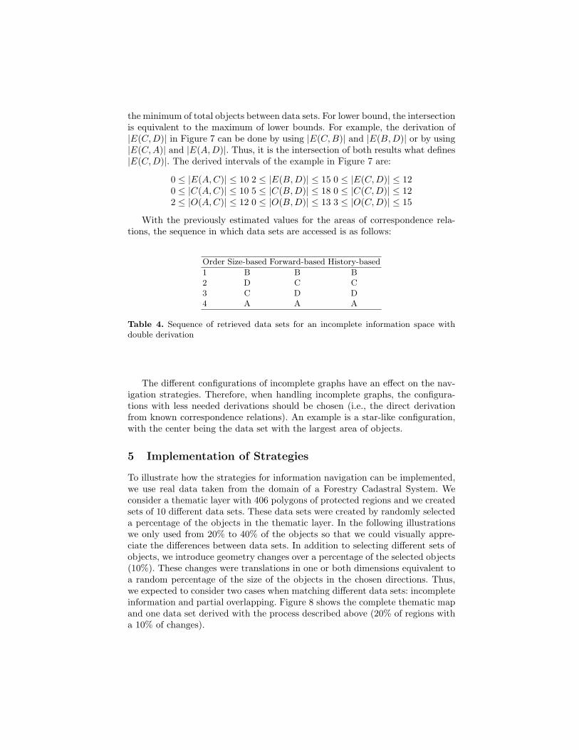
With the previously estimated values for the areas of correspondence rela-tions, the sequence in which data sets are accessed is as follows:

Order Size-based Forward-based History-based

1 B B B2 D C C3 C D D4 A A A

Table 4. Sequence of retrieved data sets for an incomplete information space withdouble derivation

The different configurations of incomplete graphs have an effect on the nav-igation strategies. Therefore, when handling incomplete graphs, the configura-tions with less needed derivations should be chosen (i.e., the direct derivationfrom known correspondence relations). An example is a star-like configuration,with the center being the data set with the largest area of objects.

5 Implementation of Strategies

To illustrate how the strategies for information navigation can be implemented,we use real data taken from the domain of a Forestry Cadastral System. Weconsider a thematic layer with 406 polygons of protected regions and we createdsets of 10 different data sets. These data sets were created by randomly selecteda percentage of the objects in the thematic layer. In the following illustrationswe only used from 20% to 40% of the objects so that we could visually appre-ciate the differences between data sets. In addition to selecting different sets ofobjects, we introduce geometry changes over a percentage of the selected objects(10%). These changes were translations in one or both dimensions equivalent toa random percentage of the size of the objects in the chosen directions. Thus,we expected to consider two cases when matching different data sets: incompleteinformation and partial overlapping. Figure 8 shows the complete thematic mapand one data set derived with the process described above (20% of regions witha 10% of changes).

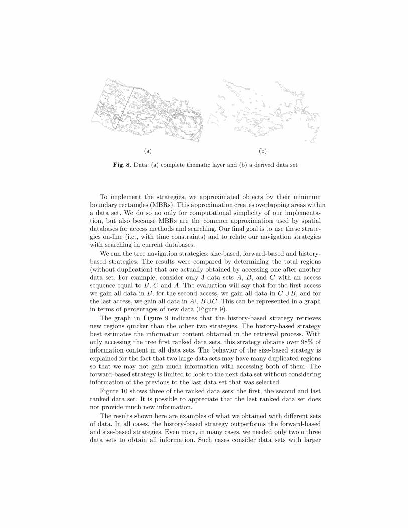
(a) (b)

Fig. 8. Data: (a) complete thematic layer and (b) a derived data set

To implement the strategies, we approximated objects by their minimumboundary rectangles (MBRs). This approximation creates overlapping areas withina data set. We do so no only for computational simplicity of our implementa-tion, but also because MBRs are the common approximation used by spatialdatabases for access methods and searching. Our final goal is to use these strate-gies on-line (i.e., with time constraints) and to relate our navigation strategieswith searching in current databases.

We run the tree navigation strategies: size-based, forward-based and history-based strategies. The results were compared by determining the total regions(without duplication) that are actually obtained by accessing one after anotherdata set. For example, consider only 3 data sets A, B, and C with an accesssequence equal to B, C and A. The evaluation will say that for the first accesswe gain all data in B, for the second access, we gain all data in C ∪ B, and forthe last access, we gain all data in A∪B∪C. This can be represented in a graphin terms of percentages of new data (Figure 9).

The graph in Figure 9 indicates that the history-based strategy retrievesnew regions quicker than the other two strategies. The history-based strategybest estimates the information content obtained in the retrieval process. Withonly accessing the tree first ranked data sets, this strategy obtains over 98% ofinformation content in all data sets. The behavior of the size-based strategy isexplained for the fact that two large data sets may have many duplicated regionsso that we may not gain much information with accessing both of them. Theforward-based strategy is limited to look to the next data set without consideringinformation of the previous to the last data set that was selected.

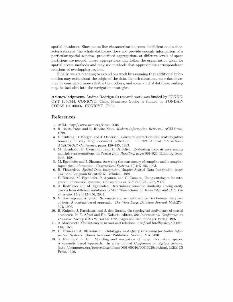
Figure 10 shows three of the ranked data sets: the first, the second and lastranked data set. It is possible to appreciate that the last ranked data set doesnot provide much new information.

The results shown here are examples of what we obtained with different setsof data. In all cases, the history-based strategy outperforms the forward-basedand size-based strategies. Even more, in many cases, we needed only two o threedata sets to obtain all information. Such cases consider data sets with larger

0,8

0,82

0,84

0,86

0,88

0,9

0,92

0,94

0,96

0,98

1

1 2 3 4 5 6 7 8 9 10

Number of databases navigated

% N

ew i

nfo

rma

tio

n

Size-based stratey

Forward-based strategy

History-base strategy

Fig. 9. Results in terms of percentages of new information

(a) (b)

(c)

Fig. 10. Ranked data sets: (a) first, (b) second, and (c) last data set

numbers of objects than the number of objects in the illustrated example and,therefore, data sets with larger numbers of duplications.

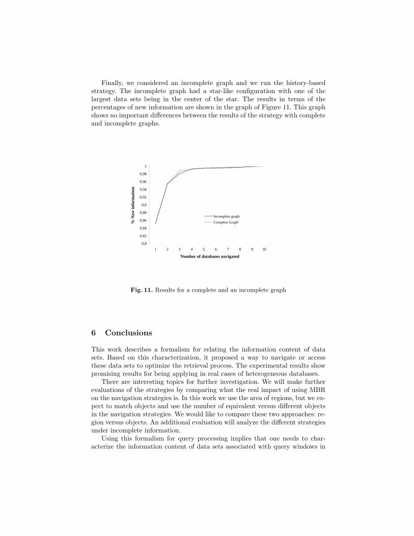
Finally, we considered an incomplete graph and we run the history-basedstrategy. The incomplete graph had a star-like configuration with one of thelargest data sets being in the center of the star. The results in terms of thepercentages of new information are shown in the graph of Figure 11. This graphshows no important differences between the results of the strategy with completeand incomplete graphs.

0,8

0,82

0,84

0,86

0,88

0,9

0,92

0,94

0,96

0,98

1

1 2 3 4 5 6 7 8 9 10

Number of databases navigated

% N

ew i

nfo

rmati

on

Incomplete graph

Complete Graph

Fig. 11. Results for a complete and an incomplete graph

6 Conclusions

This work describes a formalism for relating the information content of datasets. Based on this characterization, it proposed a way to navigate or accessthese data sets to optimize the retrieval process. The experimental results showpromising results for being applying in real cases of heterogeneous databases.

There are interesting topics for further investigation. We will make furtherevaluations of the strategies by comparing what the real impact of using MBRon the navigation strategies is. In this work we use the area of regions, but we ex-pect to match objects and use the number of equivalent versus different objectsin the navigation strategies. We would like to compare these two approaches: re-gion versus objects. An additional evaluation will analyze the different strategiesunder incomplete information.

Using this formalism for query processing implies that one needs to char-acterize the information content of data sets associated with query windows in

spatial databases. Since an on-line characterization seems inefficient and a char-acterization at the whole databases does not provide enough information of aparticular spatial window, pre-defined aggregations at different levels of spacepartitions are needed. These aggregations may follow the organization given forspatial access methods and may use methods that approximate correspondencerelations of overlapping regions.

Finally, we are planning to extend our work by assuming that additional infor-mation may exist about the origin of the data. In such situation, some databasesmay be considered more reliable than others, and some kind of database rankingmay be included into the navigation strategies.

Acknowledgment. Andrea Rodrıguez’s research work was funded by FONDE-CYT 1050944, CONICYT, Chile. Francisco Godoy is funded by FONDAP-COPAS 150100007, CONICYT, Chile.

References

1. ACM. http://www.acm.org/class. 2006.2. R. Baeza-Yates and B. Ribeiro-Neto. Modern Information Retrieval. ACM Press,

1999.3. D. Cutting, D. Karger, and J. Oederson. Constant interaction-time scatter/gather

browsing of very large document collection. In 16th Annual InternationalACM/SIGIR Conference, pages 126–135, 1993.

4. M. Egenhofer, E. Clementini, and P. Di Felice. Evaluating inconsistency amongmultiple representations. In Spatial Data Handling, pages 901–920, Edinburg, Scot-land, 1994.

5. M. Egenhofer and J. Sharma. Assessing the consistency of complete and incompletetopological information. Geographical Systems, 1(1):47–68, 1993.

6. R. Flowerdew. Spatial Data Integration, chapter Spatial Data Integration, pages375–387. Longman Scientific & Technical, 1991.

7. F. Fonseca, M. Egenhofer, P. Agouris, and C. Camara. Using ontologies for inte-grated information systems. Transactions in GIS, 6(3):231–257, 2002.

8. A. Rodrıguez and M. Egenhofer. Determining semantic similarity among entityclasses from different ontologies. IEEE Transactions on Knowledge and Data En-gineering, 15(2):442–456, 2003.

9. V. Kashyap and A. Sheth. Schematic and semantic similarities between batabaseobjects: A context-based approach. The Very Large Database Journal, 5(4):276–304, 1996.

10. B. Kuipers, J. Paredaens, and J. den Busshe. On topological equivalence of spatialdatabases. In F. Afrati and Ph. Kolaitis, editors, 6th International Conference onDatabase Theory ICDT97, LNCS 1186, pages 432–446. Springer Verlag, 1997.

11. A. Mackworth. Consistency in networks of relations. Artificial Intelligence, 8(1):99–118, 1977.

12. E. Mena and A. Illarramendi. Ontology-Based Query Processing for Global Infor-mation Systems. Kluwer Academic Publishers, Norwell, MA, 2001.

13. S. Ram and S. G. Modeling and navigation of large information spaces:A semantic based approach. In International Conference on System Science.[http://computer.org/proceedings/hicss/0001/00016/00016020abs.htm], IEEE CSPress, 1999.

14. D. Roussinov and M. McQuaid. Information navigation by clustering and summaryquery results. In International Conference on System Sciences, page 3006. IEEECS Press, 2000.

15. A. Sheth. Interoperating Geographic Information Systems, chapter Changing Focuson Interoperability in Information Systems: From System, Syntax, Structure toSemantics, pages 5–30. Kluwer Academic Plublishers, 1999.

16. VIVISMO. http://vivismo.com. 2006.17. P. Weinstein and P. Birmingham. Comparing concepts in differentiated ontologies.

In 12th Workshop on Knowledge Adquisition, Modeling, and Management, Banff,Canada, 1999.

18. M. Worboys and E. Clementini. Integration of imperfect spatial information. Jour-nal of Visual Languages and Computing, 12:61–80, 2001.

19. Yahoo! http://www.yahoo.com. 2006.20. O. Zamir and O. Etzioni. Grouper: A dynamic cluster interface to web search

results. In WWW8, 1999.