´ ECOLE NORMALE SUP ´ ERIEURE DE LYON Graph-based hierarchical knowledge representation an application to rule-based modelling and bio-curation by Eugenia Oshurko Report of M2 Internship in the PLUME team (CNRS, ENS Lyon, UCBL, LIP) under supervision of Russ Harmer Computer Science Department June 2017

Welcome message from author
This document is posted to help you gain knowledge. Please leave a comment to let me know what you think about it! Share it to your friends and learn new things together.
Transcript

ECOLE NORMALE SUPERIEURE DE LYON
Graph-based hierarchical knowledge
representation
an application to rule-based modelling and bio-curation
by
Eugenia Oshurko
Report of M2 Internship
in the
PLUME team (CNRS, ENS Lyon, UCBL, LIP)
under supervision of Russ Harmer
Computer Science Department
June 2017

Abstract
The aim of this project was to develop a framework, both conceptual and software, which
would allow coherent aggregation of fragmentary biological facts about individual protein-protein
interactions. This framework at the same time tries to solve a bio-curation problem and enables
the accommodated knowledge to be directly ‘executed’ with tools for rule-based modelling and
simulations.
Moreover, our goal was to build an expressive and mathematically robust general-purpose
knowledge representation system that can be used for building graph-based models in any domain.
As the result of our efforts, the Python library ReGraph was developed and was adopted as the
main tool for building a knowledge representation system for the specific use case of modelling
in cellular signalling.
The second part of the project was dedicated to the development of a software platform KAMI:
Knowledge Aggregator and Model Instantiator for semi-automatic aggregation and annotation of
knowledge about individual protein-protein interactions from multiple sources. This platform
also provides means for automatic instantiation of knowledge into concrete systems’ models and
their export to a rule-based modelling language Kappa.

Contents
1 Introduction and background 1
2 Knowledge representation system 2
2.1 Basic formalism . . . . . . . . . . . . . . . . . . . . . . . . . . . . . . . . . . . . . . . 2
2.2 Type respecting graph rewriting . . . . . . . . . . . . . . . . . . . . . . . . . . . . . 4
2.3 Graph hierarchy . . . . . . . . . . . . . . . . . . . . . . . . . . . . . . . . . . . . . . 5
2.4 Rewriting in a hierarchy . . . . . . . . . . . . . . . . . . . . . . . . . . . . . . . . . . 6
3 Knowledge representation for modeling of protein-protein interactions 8
3.1 Meta-model . . . . . . . . . . . . . . . . . . . . . . . . . . . . . . . . . . . . . . . . . 8
3.2 Nuggets . . . . . . . . . . . . . . . . . . . . . . . . . . . . . . . . . . . . . . . . . . . 9
3.3 Action graph . . . . . . . . . . . . . . . . . . . . . . . . . . . . . . . . . . . . . . . . 10
3.4 Semantic nuggets and semantic action graph . . . . . . . . . . . . . . . . . . . . . . 12
3.5 Hierarchy . . . . . . . . . . . . . . . . . . . . . . . . . . . . . . . . . . . . . . . . . . 13
4 Graph rewriting library ReGraph 14
4.1 Library overview . . . . . . . . . . . . . . . . . . . . . . . . . . . . . . . . . . . . . . 14
4.2 Graph hierarchy data structure . . . . . . . . . . . . . . . . . . . . . . . . . . . . . . 15
5 KAMI: Knowledge Aggregator and Model Instantiator 16
5.1 Architecture . . . . . . . . . . . . . . . . . . . . . . . . . . . . . . . . . . . . . . . . . 16
5.2 KAMI server . . . . . . . . . . . . . . . . . . . . . . . . . . . . . . . . . . . . . . . . 16
6 Conclusions 19
7 Future work 19
Appendix A Sesqui-pushout rewriting 22
Appendix B Graph hierarchy and partial homomorphisms 24
Appendix C Propagation procedure 26
Appendix D ReGraph examples 27
D.1 Simple graph rewriting with ReGraph . . . . . . . . . . . . . . . . . . . . . . . . . . 27
D.2 Graph hierarchy and rewriting in the hierarchy . . . . . . . . . . . . . . . . . . . . . 28
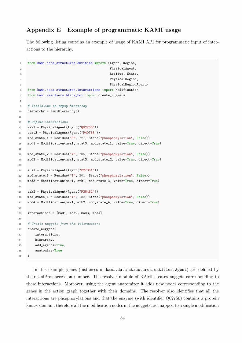
Appendix E Example of programmatic KAMI usage 34

1 Introduction and background
Knowledge about the behaviour of systems in sciences such as physics and chemistry traditionally
relies on sound models built on fundamental laws. In addition, it suffices for these models to be
a ‘good’ approximation of real phenomena. For biology, on the other hand, approaches inherited
from these sciences become infeasible due to the complexity of the systems under study. Biological
systems comprise an enormous numbers of hierarchically structured agents interacting in a non-linear
fashion, which invalidates any crude approximations in the modelling of these systems [13].
Our main interest is focused on studies of cellular signalling mechanisms which underlie essential
activities of a living cell. Thousands of highly complex molecules, proteins, take part in signalling
through various protein-protein interactions (PPIs). In addition, a single protein can have multiple
post-translational modifications of amino acids in various locations. All combinations of these mod-
ifications induce a large number of physical states of a protein, which alter its behaviour in PPIs [2].
Classical techniques for modelling the evolution of chemically reacting molecules (like modelling with
ODE’s, stochastic chemical kinetics) require an explicit listing of molecular species in the system. In
the context of cellular signalling a protein in every physical state is regarded as a distinct molecular
species [11], therefore these techniques fail as a number of species grows rapidly.
Rule-based modelling is an alternative approach to modelling PPIs which overcomes the diffi-
culties associated with the combinatorial explosion in the number of protein agents [5, 8, 9]. It
represents a system as a large graph structured in a particular way and models the system’s evolu-
tion by application of a collection of graph rewriting rules which represent individual PPIs. A rule
representing a PPI states only the necessary conditions for the interaction to appear. A language
for rule-based modelling of protein interactions Kappa and a stochastic simulator KaSim have been
developed in recent years [1].
Another difficulty which arises in the studies of biological mechanisms such as cellular signalling
is also rooted in the complexity of the systems. Due to the way biological knowledge has been tradi-
tionally obtained and accumulated, it tends to be fragmentary and dispersed over multiple sources
containing only partial mechanistic details of some phenomena. Knowledge of different provenance
can also be incoherent or be valid only in some particular context. In addition, different biological
facts can have different epistemic status: they can represent experimental results, hypotheses, or be
inferred from other facts. Depending on its status every fact should be treated by a modeller in a
respective way.
Therefore, there is a need of a knowledge representation system that would be able to gradually
aggregate knowledge in a consistent way, and at the same time would allow maintaining variant
models of the system obtained from the different versions of a single or a collection of PPIs. The
aggregation of partial knowledge should be based on the understanding of the mechanisms underlying
the interactions and on the refinement of phenomenological observations with detailed mechanistic
descriptions of the interactions.
1
We would also like to build this infrastructure in a way that would enable us to directly instantiate
models in Kappa and run simulations with KaSim. This way our knowledge representation system
would not only accommodate data but also would be directly ‘executable’.
To summarize, our goal is to build a platform that implements this knowledge representation
system. The main use case lies in the systems biology field, and in particular, we are interested in
building such an infrastructure for accommodating knowledge about signalling pathways in the cell.
2 Knowledge representation system
We have built an expressive and flexible mathematical model for knowledge representation (KR)
based on category theory, that provides robust mechanisms for incremental aggregation of partial
knowledge and for its transfer to the various representations.
The main modelling units in our KR system are graphs whose nodes correspond to arbitrary
entities of the system, and edges represent relations between them (for example, hierarchical or-
ganisation of entities and so on), both equipped with dictionary attributes. Such graphs define a
modeller’s world-view on a system on some abstraction level. We keep our framework as generic as
possible and provide a sophisticated mechanism through which ‘syntax’ and ‘semantics’ of the mod-
els can be expressed. Graphical representation of the models provides us a mechanism for expressing
changes in the system, as well as changes in ‘syntax’ or ‘semantics’ with rules of graph rewriting.
Here we give the basic formalism used in the system together with the particular specification
that we adopt for the solution of curation problem for cellular signalling we stated above as the main
use-case of such KR system.
2.1 Basic formalism
First, we introduce a dictionary structure, which will be used to represent attributes assigned to
different objects in the KR system. Attributes can be used to express properties of the entities in
the system as well as to assign annotations to the accommodated facts (i.e. meta-data).
Definition 2.1. A dictionary is a function d : V → K that maps a finite set of values to a finite set
of keys, V and K here are the objects of the category Setsfin
Definition 2.2. A dictionary d1 : V1 → K1 is a subdictionary of d2 : V2 → K2 (d1 ≤ d2) if the
following square commutes:V1 K1
V2 K2
d1
f g
d2
where arrows f and g are injective maps. Intuitively, these injective maps can be seen as set inclusions
V1 ⊆ V2 and K1 ⊆ K2 up to renaming (of keys and values). This defines the dictionary inclusion
relation ≤.
2

In the category of dictionaries Dict (it is also the subcategory of monos of the arrow category
Sets→fin) the objects are dictionaries, the homomorphisms are dictionary inclusions ≤.
We would like to represent models in our KR graphically, therefore the main structure in the
KR system is a graph equipped with the dictionary attributes.
Definition 2.3. A simple graph with attributes G is defined by a tuple (V,E,AV , AE , f, g), where
V is a set of vertices, E ⊆ V × V is a set of edges, AV and AE are sets of dictionaries, a function
f : V → AV assigns a dictionary from AV to every vertex and g : E → AE assigns a dictionary from
AE to every edge of the graph.
Definition 2.4. A homomorphism on graphs with attributes G = (V G, EG, AGV , A
GE , f
G, gG) and
H = (V H , EH , AHV , AH
E , fH , gH) is defined by a mapping h : V G → V H such that:
1. If (u, v) ∈ EG, (h(u), h(v)) ∈ EH (edges are preserved).
2. For all u ∈ V G fG(u) ≤ fH(h(u)).
3. For all (u, v) ∈ EG, gG(u, v) ≤ gH(h(u), h(v)).
The latter two definitions give the objects and the arrows of the category of graphs with attributes
Graphsattrs.
We introduce a notion of typing for graphs with attributes via graph homomorphisms. Note that
for a fixed graph T the category of graphs typed by T is a slice category Graphsattrs/T for which
the following diagram commutes:
G G′
T
h
f
f ′
i. e. f = f ′ ◦ hConsider the following example of knowledge representation with two graphs G and T and a
typing of G by T via homomorphism f (represented with dashed arrows) describing simple facts
about people living and working in some cities on the figure 1.
G Alice
lives in
works in
Lyon works in Bob lives in Dijon
T Person
lives in
works in
City
f
Figure 1: Example of KR system
Graph typing G → T sends nodes of the graph G to their types represented by the nodes of
the graph T . Talking about graph typing by their homomorphisms, we often refer to G as a model
3

and to T as a meta-model in this context. Meta-model in some sense defines a ‘syntax’ for all the
graphical models it types by defining a set of allowed types (possibly with their attributes) and a
set of allowed edges between different types of nodes.
2.2 Type respecting graph rewriting
Graph rewriting is a natural way to express the evolution of the system modeled by a graph with
attributes. The category Graphsattrs has all pushouts and pullback complements over injective
morphisms, therefore we have a well-defined procedure of sesqui-pushout rewriting in this category
[7] (more details can be found in the appendix A). Rewriting procedure applies a rule of the form
L← P → R to an instance (defined by a matching morphism mL : L� G) in a given graph G. We
denote rewriting of G that produces G′ as G G′.
A single rule can have multiple instances (matching morphisms mL : L� G) in a given graph
G. If G is typed by some graph T , it can be useful, however, to define a typing of L, namely a
homomorphism fL : L → T . This typing restricts a set of possible matchings to the ones that
commute with the typing fL, i.e. f ◦mL = fL as on the diagram:
L P R
G
T
mLfL
h1 h2
f
Moreover, having a typing f : G→ T we are often interested in rewriting G G′ such that the
resulting graph G′ remains typed by T , i.e. there exists a unique f ′ : G′ → T (an object of the slice
category Graphsattrs/T ). A rule of such type-preserving rewriting is given by a span Lh1← P
h2
→ R
and a homomorphism fR : R → T that defines a typing of the right-hand side of the rule. Then
the typing G′ → T is given by the universal property of the pushout from G−� P → R (see more
details in the appendix A).
Recall the example from the figure 1 which illustrated a simple model describing facts about
people living and working in some cities. Now consider the situation when Alice is being reallocated
by her employer to another city, for example to Paris. The respective change in the system can be
done using the graph rewriting rule depicted on the figure 2.L P R
a b c a b c a b c
Paris
h1 h2
Figure 2: Example of a graph rewriting rule. This rule deletes the edge ‘b’→ ‘c’, adds a new node‘Paris’ and the edge ‘b’→ ‘Paris’.
Four different matchings L � G of this rule can be found in our system represented with the
graph G from the example 1: (1) mL(a) = Alice, mL(b) = lives in, mL(c) = Lyon; (2) mL(a) =
Alice, mL(b) = works in, mL(c) = Lyon; (3) mL(a) = Bob, mL(b) = lives in, mL(c) = Dijon; (4)
mL(a) = Bob, mL(b) = works in, mL(c) = Lyon.
4

However, we are interested in the ones where the node ‘b’ is being matched to a node of the
type ‘works in’, therefore we define the following typing fL of L by the graph T : fL(a) = Person,
fL(b) = works in, fL(c) = City. Now there exist only two possible matchings of the rule that
respect fL, namely the instances (2) and (4). Finally, to model the previously described reallocation
of Alice to Paris we rewrite instance (2). However, if we want the resulting graph to remain typed
by T , we need to explicitly provide a typing homomorphism fR of the right-hand side of the rule R
where newly added node ‘Paris’ is mapped to the node ‘City’ from the meta-model T . The figure 3
illustrates the result of such rewriting.
G′ Alice
lives in
works in
Lyon
Paris
works in Bob lives in Dijon
T Person
lives in
works in
City
f ′
Figure 3: KR system after rewriting. The result of rewriting G G′ obtained with an applicationof the rule from the figure 2 with the typing fR of the right hand-side which maps the node ‘Paris’to the node ‘City’ in T .
2.3 Graph hierarchy
The higher level construction which enables us to represent complex knowledge systems is a graph
hierarchy. A graph hierarchy is a DAG, where nodes are graphs with attributes and edges are
(partial) homomorphisms representing graph typing in the system. This construction provides means
for mathematically robust procedures of propagation of changes (expressed through graph rewriting
rules) on any level of the hierarchy, up to all the graphs which are transitively typed by the graph
subject to rewriting.
Definition 2.5. A graph hierarchy is a DAG, where nodes are objects of the category Graphsattrs,
edges represent typing homomorphisms between graphs, and for any two paths h1, h2, . . . , hn and
i1, i2, . . . , im from G1 to G2 (i.e. dom(h1) = dom(i1) = G1 and cod(hn) = cod(im) = G2), the
homomorphisms f = hn ◦ hn−1 ◦ . . . ◦ h2 ◦ h1 and g = im ◦ im−1 ◦ . . . ◦ i2 ◦ i1 (constructed with the
composition of the homomorphisms along the paths) are equal.
In practice, we also allow to explicitly accommodate in the hierarchy undirected edges repre-
senting symmetric relations between graphs, which are defined by sets of pairs of nodes. A relation
between two graphs G1 and G2 also corresponds to the span G1 ← G12 → G2, therefore can be
treated as such in the procedures of rewriting and propagation that will be defined in the next
section. Introducing relations to a graph hierarchy would be useful further for definition of domain-
specific semantic properties, as will be discussed in the section 3.
5

2.4 Rewriting in a hierarchy
In general, after rewriting G G′ in a hierarchy, the following steps should be performed: (1) an
update of the typings by all immediate successors of G; (2) a propagation of changes from G to all
the graphs in the hierarchy which are transitively typed by it; (3) an update of all the edges affected
by the rewriting. The following points give a detailed description of the respective steps.
1. Consider some graph G in a graph hierarchy and a set of its immediate successors (graphs
typing G) as in the figure below:G
T1 T2 . . . Tm−1 Tm
. . .
We want to perform a type-preserving rewriting G G′ with a rule r : L ← P → R in this
context, namely we want G′ to be typed by T1, T2, . . . , Tn after rewriting, and for this purpose
typing of R by every such successor should be provided as discussed in the previous section.
Remark 2.6. In general, we allow hierarchies to have partial typing homomorphisms (more
details can be found in the appendix B), in which case it is not required to type the right-hand
side of the rule R. If the rewriting rule creates new nodes which are not typed by some Tk
and if typing G→ Tk was total, as the result of rewriting this typing becomes partial.
2. Consider a set of graphs typed by G (both immediate predecessors and graphs typed transi-
tively via composition of homomorphisms along the path to G) H1, H2, . . . ,Hn as on the figure
below:H1 H2 . . . Hn−1 Hn
G
. . .
After rewriting G G′ we would like to propagate the changes in G to all the graphs
H1, H2, . . . ,Hn typed by it. Specifically, to preserve the coherence of the hierarchy we want to
remove and clone all the nodes (and edges) that map to the nodes in G which are respectively
removed or cloned. Adds and merges produced by the application of the rule do not affect the
graphs typed by G in the hierarchy.
For every graph Hk typed by G (immediately or transitively) and the span G ← G− → G′
produced as the result of sesqui-pushout rewriting procedure, propagation of deletions and
clones from G to Hk can be performed with the pullback from Hk → G ← G− as illustrated
on the diagram below (here and further in this section we denote with green arrows the newly
constructed homomorphisms to distinguish them from the homomorphisms initially given in
the hierarchy and denoted with black arrows):
Hk H−k
G G− G′
6
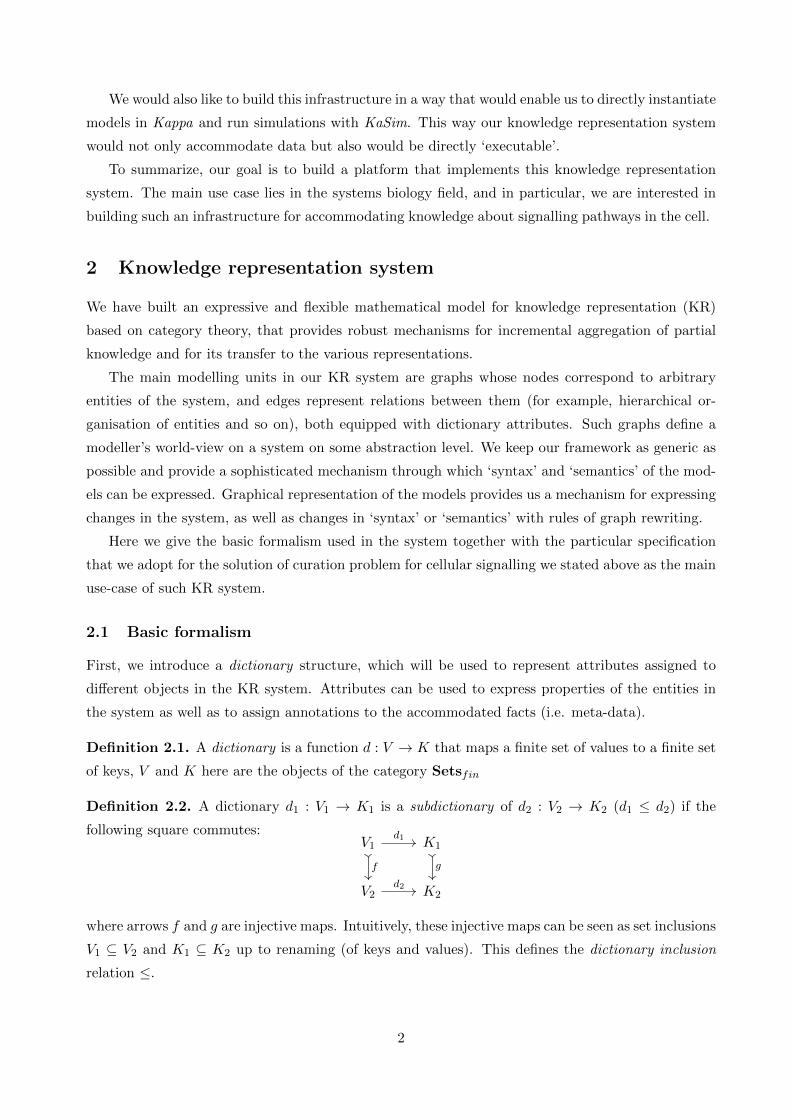
The graph H−k corresponds to the result of deletions and cloning of all the nodes in Hk which
are typed by the nodes in G that were either deleted or cloned in the course of rewriting.
3. For all Hl that type Hk, which has been affected by the previously specified propagation, the
typing is updated with the composition (Hk → Hl) ◦ (H−k → Hk) as shows the diagram below:
Hk H−k
Hl G G− G′
Consider a graph Hk typed by G via some homomorphism f1 and a graph Hl typed by Hk
via f2 (illustrated on the diagram below). Hl is typed by G not directly, but transitively
via the homomorphism constructed from the composition f1 ◦ f2. In this case propagation of
changes in G is performed similarly by finding the pullback from Hl → G← G−. However, to
preserve the initial graph structure of the hierarchy, a homomorphism f ′2 : H−l → H−k should
be found. Due to the fact that f1 ◦ f2 ◦ h2 = g ◦ u and the universal property of the pullback
Hk ← H−k → G− from Hk → G ← G−, there exists a unique homomorphism f ′2 as on the
diagram below: Hl H−l
Hk H−k
G G−
f2
h2
u
f ′2
f1
h1
f ′1
g
A special case arises when we propagate the changes to a graph whose predecessor has already
been updated. For example, consider a hierarchy with the following structure: Hk → G,
Hl → G and Hk → Hl (denoted with black arrows on the diagram below). The changes to Hk
have already been propagated (and therefore H−k has been constructed). Now we would like
to propagate the changes to Hl, and to find an updated edge H−k → H−l . H−l is constructed
the same way as previously by finding the pullback Hl ← H−l → G− from Hl → G ← G−.
From the fact that g ◦ f ′1 = f2 ◦ f3 ◦ h1 and the universal property of the pullback follows that
there exists a unique homomorphism f ′3 : H−k → H−l (denoted with red dashed arrow on the
diagram).
H−k H−l
Hk Hl
G G−
h1 f ′1
f ′3
h2
f ′2
f1
f3
f2
g
The high-level pseudocode of propagation procedure is presented in the appendix C. Starting
from the initial rewritten graph G this procedure traverses a hierarchy in the breadth-first manner
(in the reverse direction of the edges). Traversal propagates the changes to all the graphs transitively
typed by G and updates all the edges affected by the propagation.
7
3 Knowledge representation for modeling of protein-protein inter-
actions
We now present the specification of the knowledge representation system for rule-based modelling
of protein-protein interactions. This KR system is the main component of the bio-curation platform
KAMI: Knowledge Aggregator and Model Instantiator that will be presented section 5. Here we
gradually present the graphs it encapsulates as well as the functions and the relations between these
graphs, and their interpretation and usage in the rule-based modeling framework.
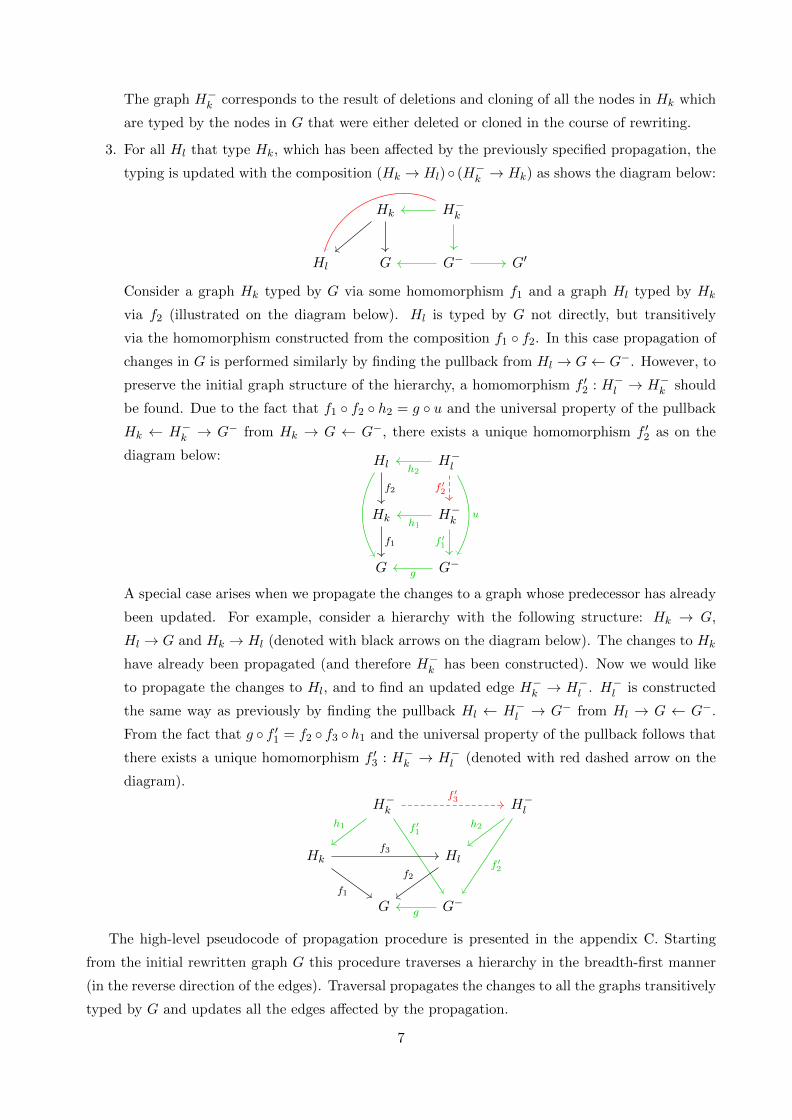
3.1 Meta-model
First we define a concrete graph M representing the meta-model for our protein-protein interaction
KR. The meta-model defines a set of agents and actions in rule-based models, as well as a set of
allowed edges between different types of nodes. The adopted meta-model (shown on the figure 4)
represents a refined version of the meta-model previously presented in [5].
Gene
Region
Residue
State
Locus
is freeis bnd
mod bnd brk
Figure 4: Graph M , the meta-model for protein-protein interaction knowledge representation
In figure 4 we schematically denote nodes corresponding to agents and their structural elements
with circular nodes, and interactions with rectangular nodes. The node State denoted with dashed
borders represents a special type of node with a unique attribute whose value can be modified during
system evolution; using nodes of this type we will express modifications of different protein states
such as phosphorylation, activity state, etc. The node Locus is another special node that, unlike
other agent nodes in the meta-model (such as Region or Residue), does not represent a physical
structural element of a protein, but serves a purely formal purpose in the meta-model, which will be
explained later. The main protein-protein interactions of interest are modification of protein states,
protein binding and breaking of protein bonds. In the meta-model these interactions are represented
explicitly by the nodes mod, bnd and brk respectively. With diamonds we denote the nodes that
we call ‘test’ nodes, and that are used to express the conditions of presence or absence of bindings.
By choosing this meta-model we build our KR system around a notion of gene as our ‘reference
entity’. From genes we can define their products (i.e. proteins) by providing specific regions, residues
8
and states. Therefore, in our system an agent actually represents not a single protein, but a feasible
‘neighbourhood in sequence space’ [5] of gene products. For example, we can specify an interaction,
for which a particular gene product should have a specific mutation of some residue, by attaching a
Residue node with a fixed value of amino acid corresponding to the mutation. More examples of
the biological facts expressed with graphs typed by the meta-model M will follow.
3.2 Nuggets
Nugget is the main unit of information in our knowledge representation system. It describes a single
biological fact, and formally it is a connected graph typed by the meta-model M . In addition,
every nugget has the following properties: (1) it contains exactly one action node (a node of the
type mod, bnd or brk); (2) any bnd and brk node has exactly two out-going edges; (4) for
every agent node in a nugget there exists a path to a gene node. The first property forces our
nuggets to contain knowledge about a single protein-protein interaction, property 2 guarantees that
the expressed interactions are semantically correct (according to the domain-specific semantics of
protein interactions), and the last one guarantees that the participating agents are grounded to their
reference gene.
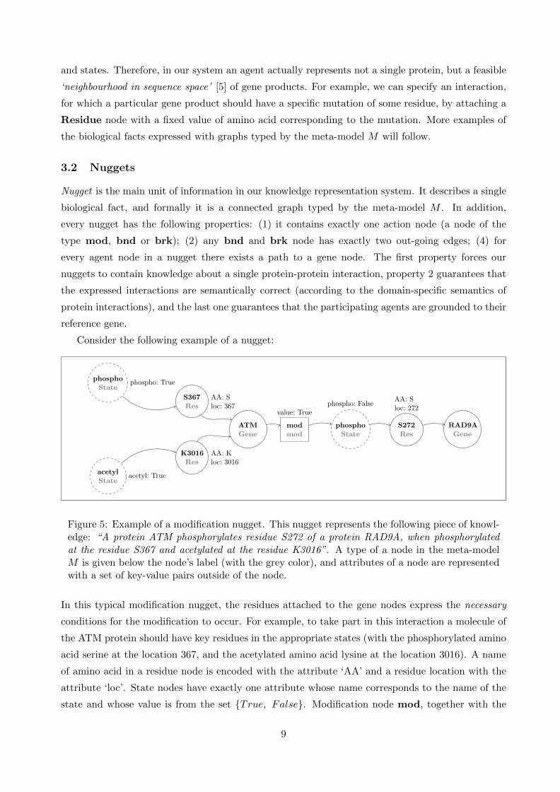
Consider the following example of a nugget:
ATMGene
S367Res
AA: Sloc: 367
phosphoState
phospho: True
K3016Res
AA: Kloc: 3016
acetylState
acetyl: True
modmod
value: True
S272Res
AA: Sloc: 272
phosphoState
phospho: False
RAD9AGene
Figure 5: Example of a modification nugget. This nugget represents the following piece of knowl-edge: “A protein ATM phosphorylates residue S272 of a protein RAD9A, when phosphorylatedat the residue S367 and acetylated at the residue K3016”. A type of a node in the meta-modelM is given below the node’s label (with the grey color), and attributes of a node are representedwith a set of key-value pairs outside of the node.
In this typical modification nugget, the residues attached to the gene nodes express the necessary
conditions for the modification to occur. For example, to take part in this interaction a molecule of
the ATM protein should have key residues in the appropriate states (with the phosphorylated amino
acid serine at the location 367, and the acetylated amino acid lysine at the location 3016). A name
of amino acid in a residue node is encoded with the attribute ‘AA’ and a residue location with the
attribute ‘loc’. State nodes have exactly one attribute whose name corresponds to the name of the
state and whose value is from the set {True, False}. Modification node mod, together with the
9

state node phospho it points to, defines an interaction represented in a nugget, namely, it states
that as the result of this interaction the phosphorylation state of the residue S272 of a molecule of
RAD9A will be set to True.
3.3 Action graph
An action graph A ~N associated with a collection of nuggets ~N (also called a pre-model in [5]) is
a graph typed by the meta-model M that types every nugget in this collection (via a respective
collection of homomorphisms ~N → A ~N ). An action graph assembles the knowledge represented in
the nuggets from ~N , and together with ~N → A ~N it specifies the interpretation of nuggets.
Having a collection of nuggets ~N = {N1, N2, . . . , Nm}, A ~N , and ~N → A ~N = {f1 : N1 → A ~N , f2 :
N2 → A ~N , . . . , fm : Nm → A ~N}, for any two nuggets Nk = (Vk, Ek) and Nl = (Vl, El), we say that
a node u ∈ Vk corresponds to a node v ∈ Vl, if they are mapped to the same node in A ~N , i.e. if
fk(u) = fl(v). For example, if two gene nodes in different nuggets map to the same gene node in an
action graph, these two nodes are interpreted as the same gene.
Note that for a given collection of nuggets we can construct multiple action graphs. Therefore,
we say that a model of a system is given by a tuple ( ~N,A ~N , ~N → A ~N ) [5], thus by a collection of
facts and their interpretation defined in terms of correspondences between agents and interactions
mentioned in these facts.
Consider two binding nuggets presented on the figure 6. These nuggets represent two rules of
protein binding. In the first one a molecule of Grb2 binds to a molecule of EGFR through the SH2
domain region, and in the second one a molecule of the same protein Grb2 binds to a molecule of
Shc through the SH2 domain.
Grb2Gene
S90Res
AA: Sloc: 90
SH2Reg
start: 60end: 135
Grb2locus
Locus
bndbnd
EGFRlocus
Locus
EGFRGene
Y1092Res
AA: Yloc: 1092
phosphoState
phospho: True
(a) Nugget N1: “Protein Grb2 with amino acid S at the location 90 binds EGFR through the SH2 domainprovided that EGFR is phosphorylated on Y1092.”
Grb2Gene
S90Res
AA: Tloc: 90
SH2Reg
start: 60end: 135
Grb2locus
Locus
bndbnd
Shclocus
Locus
ShcGene
phosphoState
phospho: True
(b) Nugget N2: “Protein Grb2 with amino acid T at the location 90 binds Shc through the SH2 domainprovided that Shc is phosphorylated.”
Figure 6: Examples of binding nuggets N1 and N2 (from [5])
10

Now consider the action graph A illustrated on the figure 7, and two functions f1 : N1 → A
and f2 : N2 → A which map the nodes from the nuggets to the action graph nodes with the
same name (labeled with bold font on the figures), except for the bnd and Grb2 locus nodes,
namely, f1(Grb2 locus) = Grb2 locus 1, f2(Grb2 locus) = Grb2 locus 2, f1(bnd) = bnd 1,
f2(bnd) = bnd 2.
Grb2Gene
S90Res
AA: {S, T}loc: 90
SH2Reg
start: 60end: 135
Grb2locus 1
Locus
Grb2locus 2
Locus
bnd 1bnd
bnd 2bnd
EGFRlocus
Locus
EGFRGene
Y1092Res
AA: Yloc: 1092
phosphoState
phospho: True
Shclocus
Locus
ShcGene
phosphoState
phospho: True
Figure 7: Action graph A
In the model ({N1, N2}, A, {f1, f2}) the interactions represented by the nuggets are interpreted
in such a way that two bindings can happen at the same time, namely a molecule of Grb2 can
bind both EGFR and Shc at the same time, creating the Grb2/EGFR/Shc complex. Now, consider
another action graph A′ depicted on the figure 8 and the functions f ′1 : N1 → A′ and f ′2 : N2 → A′
for which f ′1(EGFR locus) = EGFR/Shc locus and f ′2(Shc locus) = EGFR/Shc locus, and
all the other nodes are mapped to the action graph nodes with the same name.
Grb2Gene
S90Res
AA: {S, T}loc: 90
SH2Reg
start: 60end: 135
Grb2locus
Locus
bndbnd
EGFR/Shclocus
Locus
EGFRGene
Y1092Res
AA: Yloc: 1092
phosphoState
phospho: True
ShcGene
phosphoState
phospho: True
Figure 8: Action graph A′
In the model ({N1, N2}, A′, f ′1, f ′2) the biological facts represented by the nuggets are interpreted
in a different way: a molecule of Grb2 can bind either EGFR or Shc, but not both at the same
time, as the bindings use the same locus and so the two interactions are conflicting. For this set of
11
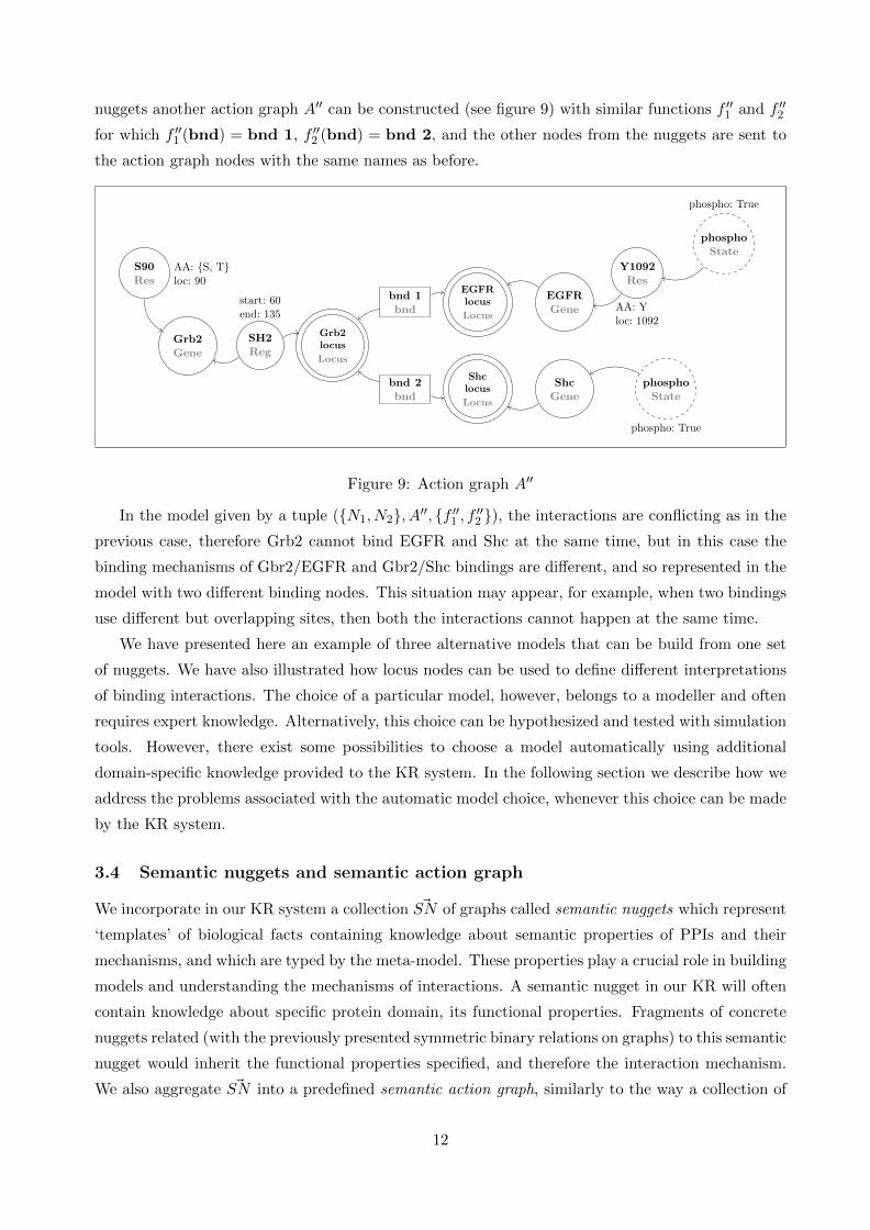
nuggets another action graph A′′ can be constructed (see figure 9) with similar functions f ′′1 and f ′′2
for which f ′′1 (bnd) = bnd 1, f ′′2 (bnd) = bnd 2, and the other nodes from the nuggets are sent to
the action graph nodes with the same names as before.
Grb2Gene
S90Res
AA: {S, T}loc: 90
SH2Reg
start: 60end: 135
Grb2locus
Locus
bnd 1bnd
bnd 2bnd
EGFRlocus
Locus
EGFRGene
Y1092Res
AA: Yloc: 1092
phosphoState
phospho: True
Shclocus
Locus
ShcGene
phosphoState
phospho: True
Figure 9: Action graph A′′
In the model given by a tuple ({N1, N2}, A′′, {f ′′1 , f ′′2 }), the interactions are conflicting as in the
previous case, therefore Grb2 cannot bind EGFR and Shc at the same time, but in this case the
binding mechanisms of Gbr2/EGFR and Gbr2/Shc bindings are different, and so represented in the
model with two different binding nodes. This situation may appear, for example, when two bindings
use different but overlapping sites, then both the interactions cannot happen at the same time.
We have presented here an example of three alternative models that can be build from one set
of nuggets. We have also illustrated how locus nodes can be used to define different interpretations
of binding interactions. The choice of a particular model, however, belongs to a modeller and often
requires expert knowledge. Alternatively, this choice can be hypothesized and tested with simulation
tools. However, there exist some possibilities to choose a model automatically using additional
domain-specific knowledge provided to the KR system. In the following section we describe how we
address the problems associated with the automatic model choice, whenever this choice can be made
by the KR system.
3.4 Semantic nuggets and semantic action graph
We incorporate in our KR system a collection ~SN of graphs called semantic nuggets which represent
‘templates’ of biological facts containing knowledge about semantic properties of PPIs and their
mechanisms, and which are typed by the meta-model. These properties play a crucial role in building
models and understanding the mechanisms of interactions. A semantic nugget in our KR will often
contain knowledge about specific protein domain, its functional properties. Fragments of concrete
nuggets related (with the previously presented symmetric binary relations on graphs) to this semantic
nugget would inherit the functional properties specified, and therefore the interaction mechanism.
We also aggregate ~SN into a predefined semantic action graph, similarly to the way a collection of
12
~N is aggregated in the action graph A in the previous section, and relate the action graph to the
semantic action graph.
Semantic nuggets help us to (1) check that an input interaction is semantically correct; (2)
autocomplete nuggets with more mechanistic details if required; (3) impose constraints on the action
graph (which helps us to build and constrain the models).
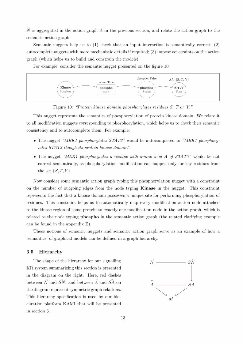
For example, consider the semantic nugget presented on the figure 10:
KinaseRegion
phosphomod
value: True
S,T,YRes
AA: {S, T, Y}
phosphoState
phospho: False
Figure 10: “Protein kinase domain phosphorylates residues S, T or Y.”
This nugget represents the semantics of phosphorylation of protein kinase domain. We relate it
to all modification nuggets corresponding to phosphorylation, which helps us to check their semantic
consistency and to autocomplete them. For example:
• The nugget “MEK1 phosphorylates STAT3” would be autocompleted to “MEK1 phosphory-
lates STAT3 though its protein kinase domain”.
• The nugget “MEK1 phosphorylates a residue with amino acid A of STAT3” would be not
correct semantically, as phosphorylation modification can happen only for key residues from
the set {S, T, Y }.
Now consider some semantic action graph typing this phosphorylation nugget with a constraint
on the number of outgoing edges from the node typing Kinase in the nugget. This constraint
represents the fact that a kinase domain possesses a unique site for performing phosphorylation of
residues. This constraint helps us to automatically map every modification action node attached
to the kinase region of some protein to exactly one modification node in the action graph, which is
related to the node typing phospho in the semantic action graph (the related clarifying example
can be found in the appendix E).
These notions of semantic nuggets and semantic action graph serve as an example of how a
‘semantics’ of graphical models can be defined in a graph hierarchy.
3.5 Hierarchy
The shape of the hierarchy for our signalling
KR system summarizing this section is presented
in the diagram on the right. Here, red dashes
between ~N and ~SN , and between ~A and ~SA on
the diagram represent symmetric graph relations.
This hierarchy specification is used by our bio-
curation platform KAMI that will be presented
in section 5.
~N ~SN
A SA
M
13
4 Graph rewriting library ReGraph
The previous two sections presented the formalism for graph-based hierarchical KR and its speci-
fication for modelling individual PPIs. The following two sections present the generic software im-
plementing the formalism and the platform for accommodating and managing the domain-specific
graph hierarchy for rule-based modelling of PPIs.
In collaboration with other interns and post-docs involved in the project I started working on
the Python library for graph rewriting ReGraph during my M1 internship. By the beginning of the
M2 internship ReGraph contained data structures and functionality necessary for the basic rewriting
and knowledge representation purposes.
ReGraph implements a general-purpose framework for modelling graph-based systems, and is the
main tool used for building our domain-specific knowledge infrastructure. Most of the functionality of
the library uses graph data structures from the NetworkX library for graph manipulation (hereafter
we refer to this as nx), which is widely used in the network science community and contains a
great number of implemented algorithms on graphs. ReGraph provides various utilities for graph
rewriting which can be used for modelling the evolution of a system represented by a graph subject
to rewriting. The rewriting functionality is based on the sesqui-pushout rewriting procedure [7]. In
addition, the library enables a user to define a typing for models (graphs) that gives specifications for
the structure of the models. This later functionality allows both to preserve the specified structure
during rewriting and to propagate the changes to the specifications up to the models.
However, in order to make our knowledge infrastructure more powerful, a substantial refactoring
of ReGraph was required. The main goal of this refactoring was to make the functionality more
general, more flexible and, most importantly, more rigorous from the mathematical point of view.
The major novelty of the new version of ReGraph lies in replacing the rigid typing structure
introduced by Typed(Di)Graph with a DAG-like structure implementing a typing hierarchy, where
a directed edge is a typing homomorphisms between two graphs. The following section will detail
the data structures and the functionality developed during this refactoring process. The source code
of the library can be found by the following link https://github.com/Kappa-Dev/ReGraph. Also
a short tutorial can be found by the link1.
4.1 Library overview
ReGraph contains a collection of utilities for graph rewriting on nx graph objects, both undirected
graphs (nx.Graph) and directed ones (nx.DiGraph). The library consists of the following main
modules:
• regraph.primitives contains a set of functions for manipulating nx graphs (slightly extends
the functionality provided by nx.Graph and nx.DiGraph). In addition, provides functions for
finding subgraph matching in a graph (regraph.primitives.find matching) and rewriting
of a graph with a rule (regraph.primitives.rewrite). Subgraph matching procedure uses
1https://github.com/Kappa-Dev/ReGraph/blob/master/examples/ReGraph_demo.ipynb
14

nx.networkx.algorithms.isomorphism.(Di)GraphMatcher class which provides the method
for subgraph isomorphism finding based on the VF2 algorithm [6]. The rewriting function
implements sesqui-pushout rewiting.
• regraph.rules provides the data structure for representation of graph rewriting rules
regraph.rules.Rule, which encapsulates the rule span L ← P → R used in sesqui-pushout
rewriting. In addition, it provides an interface for gradual creation of rules from a pattern
graph (left-hand side L) in an imperative way by either invoking primitive methods (methods
corresponding to individual actions on the pattern like addition of nodes, cloning of nodes, etc.)
or providing a respective list of commands (following a simple grammar for specifying graph
transformations that can be parsed by regraph.parser).
• regraph.category contains a set of various category theory operations on graphs with at-
tributes and their homomorphisms used in sesqui-pushout rewriting and propagation in a graph
hierarchy, such as pullback, pushout, pullback complement, etc. It also provides functions
for checking validity of graph homomorphisms and functions for finding unique maps by the
universal property of pullbacks.
• regraph.hierarchy provides an implementation of the graph hierarchy data structure (more
details follow in the section 4.2).
Some examples of ReGraph usage can be found in the appendix D.
4.2 Graph hierarchy data structure
Graph hierarchy, the specification of which was presented in the section 2.3, is implemented in
regraph.hierarchy.Hierarchy (hereafter we refer to it as Hierarchy) data structure. Essentially,
the data structure is a DAG. It inherits the nx.DiGraph class, therefore all the functionality for
manipulating directed graphs can be applied to the hierarchy. Additionally, during the initialization
and addition of edges, an instance of Hierarchy is checked to be acyclic and to respect the property
of commuting paths from the same source to the same target.
Hierarchy supports two types of nodes: regraph.hierarchy.GraphNode and
regraph.hierarchy.RuleNode, thus we slightly extend the structure from the section 2.3 by allowing
to incorporate rewriting rules in a hierarchy as well. Rules are typed by edges which contain two
typing homomorphisms corresponding to the left-hand side typing and the right-hand side typing.
No nodes are allowed to be typed by a rule node, therefore during construction of the hierarchy
and addition of edges Hierarchy forbids incoming edges for rule nodes. Incorporating rules into
the hierarchy allows us to propagate changes to all the rules typed by a graph subject to rewriting,
which is useful for rules that have to remain coherent with their meta-models during the modelling
process.
Edges in a hierarchy are directed and represent typing homomorphisms. Two types of edges are
allowed in the hierarchy: regraph.hierarchy.Typing (typing of a graph by another graph) and
regraph.hierarchy.RuleTyping (typing of a rule by a graph, which includes left-hand side typing
15

and right-hand side typing). We also introduce another type of edges between the nodes representing
graph relations (regraph.hierarchy.GraphRelation). Relational edges are undirected, and are
treated separately from the typing edges in the hierarchy.
5 KAMI: Knowledge Aggregator and Model Instantiator
KAMI: Knowledge Aggregator and Model Instantiator is a semi-automatic bio-curation platform
which provides a user with tools for gradual aggregation of biological facts about individual protein-
protein interactions of different provenance, their annotation, visualisation and further instantiation
for building rule-based models of concrete systems and performing hypothesis testing.
The platform allows to input annotated biological facts through the graphical interface or pro-
grammatically through the API. The input facts can be automatically merged with an existing model
in a context-dependent manner (the knowledge present in the model influences the way these facts
are interpreted and, therefore, merged with the model). The model itself is a graph hierarchy (an
instance of ReGraph’s core data structure). Apart from the user input knowledge, the hierarchy con-
tains expert knowledge used by KAMI for the interpretation of interactions, for example, definitions
of protein families, protein variants definitions, the semantics of particular protein domains. This
expert knowledge is obtained from both publicly available data (such as UniProt, Pfam, InterPro
databases) and from collaboration with biologists. From the knowledge aggregated by a user in the
hierarchy, KAMI allows to automatically instantiate models expressed with Kappa rules and perform
simulations with KaSim. The source code of the library can be found by in the repository by the
link2.
5.1 Architecture
We have designed KAMI as a server-client application, where the server accommodates the hierarchy
presented in the section 3.5, and contains a set of tools for accessing and manipulating the hierar-
chy, instantiating concrete models, and automatically resolving input knowledge for aggregation to
the hierarchy. The client part of KAMI provides the graphical user interface and the application
programming interface (API), as well as tools for the import of knowledge from various biological
data formats. Figure 11 illustrates a schematic architecture of the main modules of KAMI and their
relationships.
5.2 KAMI server
A web-server application for KAMI is being implemented by my collaborator Yves-Stan Le Cornec
using Python micro-framework Flask. It follows a paradigm of thin-client and encapsulates the ma-
jority of functionality for manipulating the KAMI hierarchy. The server-side of KAMI incorporates
several modules which are able to perform various tasks related to the automatic aggregation and
instantiation of knowledge.
2https://github.com/Kappa-Dev/KAMI-python
16

Figure 11: High-level architecture of modules in KAMI
My main contribution to the KAMI project during the internship concerns the implementation of
an import from different biological data formats (currently the INDRA [12] importer is implemented)
and the development of a resolver of protein-protein interactions, which is able to automatically
aggregate individual facts into the existing hierarchy.
Resolver
The main purpose of the resolver module is, provided an input protein-protein interaction, to be
able to automatically:
1. create a nugget graph that respects the meta-model and corresponds to the most detailed mech-
anistic description possible of the interaction (including the interpretation of phenomenological
interactions, auto-completion of nuggets);
2. identify genes, regions, residues and states mentioned in the interaction and map the corre-
sponding nugget nodes to the ones in the existing action graph; alternatively, if the corre-
sponding nodes do not exist in the action graph, the resolver is able to add new nodes to the
action graph;
3. disambiguate and identify the interaction and map it into the corresponding node in the action
graph. For binding interactions, in particular, the resolver should identify the interaction
together with all the loci attached to it (as in the example from 3.3);
4. finally, add the nugget together with its typing by the action graph to the hierarchy.
17

For the purposes of input knowledge representation a set of intermediate data structures was im-
plemented (in kami.data structures.entites and kami.data structures.interactions mod-
ules). These data structures represent biological entities of interest and their interactions. They
serve both as the bridge between the input representation formats and our graphical representation,
and as the unified interface for programmatic input of knowledge to KAMI. The idea behind these
data structures is similar to the one of Statements in INDRA: Integrated Network and Dynamical
Reasoning Assembler (a project tangent to KAMI) [12]. INDRA provides a set of tools for reading
biological facts expressed with natural language and other formats like BioPAX [10] and represent-
ing these facts with a set of computable statements. As was mentioned earlier, we also implement
an importer which is able to convert INDRA statements to the respective KAMI data structures
(kami.importers.indra to kami).
The KAMI data structures for entities and interactions of interest differ from the INDRA state-
ments in a couple of crucial points. The first important difference is that INDRA statements cannot
represent the protein domains involved in the interactions, whereas in KAMI they play an important
role in the identification of interaction mechanisms and their interpretation. In addition, KAMI is
focused on the specific level of mechanistic details related to the interaction, which is in some cases
does not coincide with such level of INDRA knowledge representation. For example, using the IN-
DRA statement of the type indra.statements.Complex we can represent a formation of the protein
complex A/B/C (from the respective proteins A, B, C). On the other hand, to be able to input this
fact to KAMI we need to provide a direct binary binding mechanisms involved in the formation of
this complex (e.g. A binds B, and B binds C). Therefore, a direct import into KAMI data structures
from the input sources would prevent us from losing the pertinent information about mechanistic
details of interactions.
The sub-module kami.resolvers.generators contains a set of tools for generating nuggets
from the KAMI interaction objects. A generator takes as an input a particular interaction object,
and outputs a nugget together with its typing by the meta-model and the action graph. It does it
in three steps:
• build a nugget graph and type it by the meta-model;
• use anatomizer (the kami.anatomizer module) to identify genes, regions, residues and states;
• use semantic nuggets ~SN from the hierarchy to identify the interactions, and autocomplete
the nugget with more mechanistic details if necessary.
The kami.anatomizer module implemented by our biologist collaborator Sebastien Legare en-
capsulates a set of client utilities for collecting information of interest from the biological databases.
This tool plays a crucial role for identification of standardized gene and protein domains references
which carry functional annotations.
To disambiguate and identify an interaction we need to be able to understand the mechanism
that underlies it. For this purpose KAMI tries to relate an input nugget with a semantic nugget
from ~SN as it was presented in 3.4. Once the relation was established, the nugget is checked to be
18
semantically correct (otherwise discarded), then autocompleted, and finally its action is mapped to
an existing action node in the action graph related to the corresponding semantic action. A small
example of programmatic input of interactions into KAMI model is presented in the appendix E.
We have tested the resolver on a real-world dataset (PID: the pathway interaction database [14]
converted to the INDRA statements from its initial BioPAX format) containing 1724 phosphory-
lation modifications with no domains specified. As the result, 1724 nuggets were created, 1322 of
which where successfully autocompleted with the identified protein kinase region and related to
the phosphorylation semantic nugget. Aggregation of this knowledge resulted in the action graph
with 2312 nodes (including all the regions found for every gene by the anatomizer), among which
only 95 were modification nodes. It means that all 1322 phosphorylation modification nodes in the
nuggets (with the unique protein kinase region found) were identified and classified into 95 distinct
phosphorylation activities. Among the top three modification nodes with the highest number of out-
going edges in the action graph (which represents distinct genes that can be phosphorylated), the
modifications performed by the genes belonging to the Mitogen-activated protein kinase superfamily
of proteins were found (MAPK3 phosphorylates products of 57 distinct genes, MAPK14 – 56, and
MAPK1 – 54).
6 Conclusions
In this report I have presented the results of my M2 internship in the ongoing project dedicated to the
development of a graph-based hierarchical knowledge representation system for rule-based modeling
of cellular signaling. We are developing both a formalism and software tools implementing it (the
ReGraph library). Despite the fact that it is inspired and driven by the problem of bio-curation in
cellular signalling, we tried to make it as generic as possible and potentially applicable for modelling
of graph-based systems in any domain.
Another direction of our work is focused on the developments of a concrete specification of this
KR system for purposes of modelling of protein-protein interactions and a tool which would be able
to accommodate and manage it (the KAMI platform). In addition, this tool allows coherent aggrega-
tion of fragmentary biological facts about individual protein-protein interactions and encapsulates a
machinery for specific to cellular signalling automated reasoning about interaction mechanisms based
on expert knowledge. KAMI aims to facilitate the modelling processes for biologists. At the same
time time tries to solve a bio-curation problem, serves as a modelling environment and enables the
accommodated knowledge to be directly ‘executed’ and analyzed with tools for rule-based modeling
and simulations.
7 Future work
In the short-term future, there are several things should be implemented for the KAMI platform.
First, we would like to implement a set of importers which would support biological formats such
as BioPAX, and existing tools for signalling-specific natural language processing, such as TRIPS
19

[3] or REACH [15]. Potentially, we would also like to implement our own tools for processing of
biochemical literature, which would be able to extract relevant knowledge with the high accuracy
and the required level of mechanistic details (but it goes beyond our short-term goals).
Another crucial part of KAMI that requires a substantial amount of further work is the resolver.
We would like to provide a better support for aggregation and autocompletion of nuggets, and
mechanistic interpretation of phenomenological knowledge. For this purpose, we need to acquire
more semantic nuggets, and at the moment, it remains a bottleneck as the acquisition and the hard-
wiring of semantic nuggets in our system requires deep expert knowledge. However, the number of
semantic nuggets covering most of the common binding and modification mechanisms is rather small
and remains feasible for our application.
In the long term future, we would like to make KAMI not only a tool for ‘smart’ knowledge
aggregation but a full-blown modelling environment, which provides means for visualization, so-
phisticated annotation, hypothesis testing and assertions. In addition, KAMI should be able to
accommodate model variants, support the simultaneous development of multiple models and their
automated merge (similar to version control systems).
Our goal is to build a powerful modelling tool for the biological community, which by automating
the curation process would leave biologists room for experimenting, hypothesizing, discovering new
knowledge and understanding complex signalling mechanisms.
Acknowledgements
I would like to express my gratitude to my supervisor Russ Harmer for his motivation, support, trust
and guidance throughout the internship. I also would like to thank my collaborators Yves-Stan Le
Cornec and Sebastien Legare for their help, valuable advice and fruitful discussions.
This work was sponsored by the Defense Advanced Research Projects Agency (DARPA) and the
U.S. Army Research Office under grant numbers W911NF-14-1-0367 and W911NF-15-1-0544. The
views, opinions, and/or findings contained in this report are those of the authors and should not be
interpreted as representing the official views or policies, either expressed or implied, of the Defense
Advanced Research Projects Agency or the Department of Defense.
20
References
[1] KaSim Development Homepage. http://dev.executableknowledge.org/.
[2] B. Alberts, A. Johnson, J. Lewis, M. Raff, K. Roberts, and P. Walter. Molecular biology of the
cell. new york: Garland science; 2002. Classic textbook now in its 5th Edition, 2010.
[3] J. Allen, W. de Beaumont, L. Galescu, and C. M. Teng. Complex event extraction using drum.
ACL-IJCNLP 2015, page 1, 2015.
[4] S. Awodey. Category theory. Oxford University Press, 2010.
[5] A. Basso-Blandin, W. Fontana, and R. Harmer. A knowledge representation meta-model for
rule-based modelling of signalling networks. arXiv preprint arXiv:1603.01488, 2016.
[6] L. P. Cordella, P. Foggia, C. Sansone, and M. Vento. A (sub) graph isomorphism algorithm
for matching large graphs. IEEE transactions on pattern analysis and machine intelligence,
26(10):1367–1372, 2004.
[7] A. Corradini, T. Heindel, F. Hermann, and B. Konig. Sesqui-pushout rewriting. In International
Conference on Graph Transformation, pages 30–45. Springer, 2006.
[8] V. Danos, J. Feret, W. Fontana, R. Harmer, and J. Krivine. Rule-based modelling of cellular
signalling. In International Conference on Concurrency Theory, pages 17–41. Springer, 2007.
[9] V. Danos, J. Feret, W. Fontana, R. Harmer, and J. Krivine. Rule-based modelling and model
perturbation. In Transactions on Computational Systems Biology XI, pages 116–137. Springer,
2009.
[10] E. Demir, M. P. Cary, S. Paley, K. Fukuda, C. Lemer, I. Vastrik, G. Wu, P. D’Eustachio,
C. Schaefer, J. Luciano, et al. Biopax–a community standard for pathway data sharing. Nature
biotechnology, 28(9):935, 2010.
[11] D. T. Gillespie. Stochastic simulation of chemical kinetics. Annu. Rev. Phys. Chem., 58:35–55,
2007.
[12] B. M. Gyori, J. A. Bachman, K. Subramanian, J. L. Muhlich, L. Galescu, and P. K. Sorger. From
word models to executable models of signaling networks using automated assembly. bioRxiv,
page 119834, 2017.
[13] A. Moreno, K. Ruiz-Mirazo, and X. Barandiaran. The impact of the paradigm of complexity
on the foundational frameworks of biology and cognitive science. Handbook of the philosophy of
science, pages 311–333, 2011.
[14] C. F. Schaefer, K. Anthony, S. Krupa, J. Buchoff, M. Day, T. Hannay, and K. H. Buetow. Pid:
the pathway interaction database. Nucleic acids research, 37(suppl 1):D674–D679, 2009.
[15] M. A. Valenzuela-Escarcega, G. Hahn-Powell, and M. Surdeanu. Description of the odin event
extraction framework and rule language. arXiv preprint arXiv:1509.07513, 2015.
21

Appendix A Sesqui-pushout rewriting
Sesqui-pushout (SqPO) rewriting is an approach for abstract deterministic rewriting in any category
with pushouts and all pullback complements over monos [7]. We denote informally rewriting of a
graph G as G G′, where G′ is a result of rewriting. In our context, SqPO allows to perform
the following operations on graphs: addition/deletion of the nodes, addition/deletion of the edges,
cloning and merging of the nodes.
Any sequence of these operations can be expressed with a rewriting rule which is defined by a
span L ← P → R, where L represents a pattern that is going to be matched in G. An instance of
a rule is a matching morphism L� G, SqPO procedure performs rewriting of the instance in two
steps:
1. Perform all the deletions and cloning by constructing a graph G− as a final pullback comple-
ment from P → L� G.
2. Build the graph G′ as a pushout from the span G− ← P → R containing all the nodes and
edges added by the rule as well as merges of the nodes.
The diagram below illustrates the constructs used in the rewriting procedure from G to G′:
L P R
G G− G′
h1
h2
Informally application of a rule L ← P → R can be reformulated as follows (in this canonical
order):
1. Deletion of nodes: if node nL in L does not have a preimage in h1 : P → L, node in G
mapped by nL in L� G is going to be deleted by the rewriting (together with all its adjacent
edges as a side effect).
2. Deletion of edges: for h1 : P → L, if nL1 = h1(n
P1 ), and nL
2 = h1(nP2 ), and there is an edge
between nL1 and nL
2 in L, and there is no edge between nP1 and nP
2 in P , the edge in G between
nodes mapped by nL1 and nL
2 in L� G will be deleted.
3. Cloning of nodes: if two nodes nP1 , n
P2 of P map to the same node nL in L, node in G
mapped by nL in L� G is going to be cloned during graph rewriting.
4. Merging of nodes: if two nodes of nP1 and nP
2 in P match to the same node nR in R,
corresponding nodes in G are merged.
5. Addition of nodes: if node nR in R does not have a preimage in h2 : P → R, nR is going to
be added by the rewriting.
6. Addition of edges: for h2 : P → R, if nR1 = h2(n
P1 ), and nR
2 = h2(nP2 ), and there is an edge
between nR1 and nR
2 in R, and there is no edge between nP1 and nP
2 in P , the edge between
corresponding nodes in G will be added.
22

A rule L← P → R is typed by T iff L, P and R are typed by T s.t.
L P R
T
= =
The result of rewriting G G′ with a rule r : L ← P → R, where G and r are typed by T , is
also typed by T . The following proposition illustrates this fact.
Proposition A.1. There exists a unique typing f ′ : G′ → T , where G′ is the result of G G′
sesqui-pushout rewriting of a graph G with a rule Lh1← P
h2
→ R with fR : R→ T (typing of R by T )
on an instance mL : L� G.
Proof. In the first step of rewriting graph G−
is obtained from the final pullback complement
from P → L � G. G− is typed by T by the
homomorphism f ◦ g1 as illustrated on the dia-
gram. In the second step of rewriting, G′ is ob-
tained with the pushout from the span G− �
P → R, and there exists a unique homomor-
phism f ′ : G′ → T , which follows from the uni-
versal property of the pushout and the fact that
f ◦ g1 ◦mP = fR ◦ h2, as it is illustrated on the
diagram.
L P R
G G− G′
T
mL
h1 h2
mP mR
fR
fg1
g2
f ′
23

Appendix B Graph hierarchy and partial homomorphisms
Partial graph homomorphisms
To make our knowledge representation system more flexible we allow partial typing of graphs defined
by a partial homomorphism A ⇀ B in a graph hierarchy. Intuitively, partial typing does not require
for all nodes of A to be typed by nodes in B.
Definition B.1. Partial homomorphism f : A ⇀ B approximates g : A ⇀ B (f ≤ g) iff for all
x ∈ A, if f(x) is defined and f(x) = y, then g(x) is also defined and g(x) = y.
Definition B.2. Partial homomorphisms f : A ⇀ B and g : A ⇀ B are “Kleene equal” (f ' g) iff
f ≤ g and g ≤ f .
Our category of Graphsattrs is a category with pullbacks, therefore a partial homomorphism
f : A ⇀ B can be defined as the span A� AB → B, where AB is the domain of f and composition
is defined by pullback. Note that a total homomorphism is a special case of a partial one, namely a
homomorphism f : A→ B can be expressed as the span Aid� A→ B.
In terms of spans the fact that f : A ⇀ B approximates g : A ⇀ B can be reformulated as
follows. f ≤ g iff there exists a monomorphism u such that f1 = g1 ◦ u and f2 = g2 ◦ u, as shown on
the diagram below:
A
AfB Ag
B
B
f g
f1
f2
u
g1
g2
In a hierarchy with partial typing we require that any two homomorphisms f and g constructed
with the composition of the homomorphisms along the paths from A to B to be “Kleene equal”:
A
. .
. . . . . .
B
h1 i1
f g'h2 i2
hn im
Propagation to partially typed graphs
Recall in a graph hierarchy we would like to propagate the result of rewriting G G′ to all the
graphs typed by G. Previously we have considered the procedure of propagation in case of total
typing. If some graph Hk in a hierarchy is partially typed by G (Hk ⇀ G) the propagation of
changes from G to Hk is performed similarly with the pullback from Hk ⇀ G← G−.
24
Hk H−k
G G−
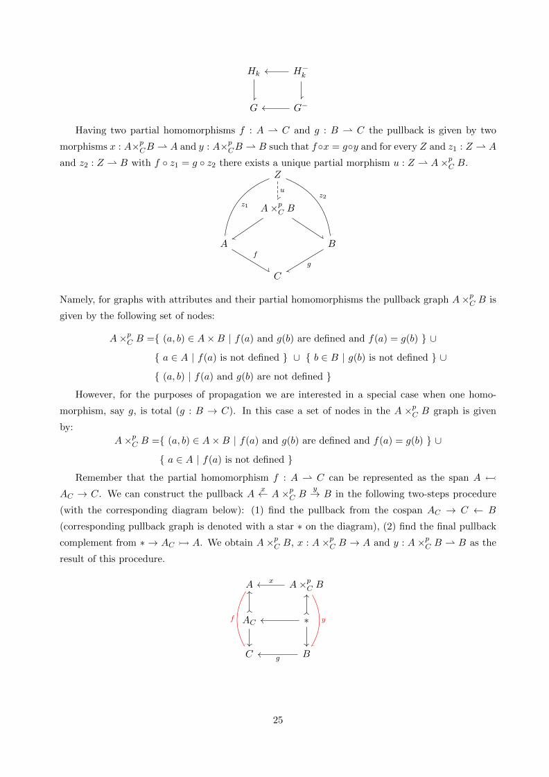
Having two partial homomorphisms f : A ⇀ C and g : B ⇀ C the pullback is given by two
morphisms x : A×pCB ⇀ A and y : A×p
CB ⇀ B such that f◦x = g◦y and for every Z and z1 : Z ⇀ A
and z2 : Z ⇀ B with f ◦ z1 = g ◦ z2 there exists a unique partial morphism u : Z ⇀ A×pC B.
Z
A×pC B
A B
C
z1
z2u
f
g
Namely, for graphs with attributes and their partial homomorphisms the pullback graph A×pC B is
given by the following set of nodes:
A×pC B ={ (a, b) ∈ A×B | f(a) and g(b) are defined and f(a) = g(b) } ∪
{ a ∈ A | f(a) is not defined } ∪ { b ∈ B | g(b) is not defined } ∪
{ (a, b) | f(a) and g(b) are not defined }
However, for the purposes of propagation we are interested in a special case when one homo-
morphism, say g, is total (g : B → C). In this case a set of nodes in the A ×pC B graph is given
by:
A×pC B ={ (a, b) ∈ A×B | f(a) and g(b) are defined and f(a) = g(b) } ∪
{ a ∈ A | f(a) is not defined }
Remember that the partial homomorphism f : A ⇀ C can be represented as the span A �
AC → C. We can construct the pullback Ax← A ×p
C By→ B in the following two-steps procedure
(with the corresponding diagram below): (1) find the pullback from the cospan AC → C ← B
(corresponding pullback graph is denoted with a star ∗ on the diagram), (2) find the final pullback
complement from ∗ → AC � A. We obtain A×pC B, x : A×p
C B → A and y : A×pC B ⇀ B as the
result of this procedure.
A A×pC B
AC ∗
C B
f
x
y
g
25

Appendix C Propagation procedure
Data: G,G−, G− → G
Result: (V,E), where V is a set of updated graphs, E is a set of updated typing
homomorphisms
V := {G−};E := ∅;visited := ∅;current level := predecessors(G);
while current level 6= ∅ do
next level := ∅;for H ∈ current level do
visited := visited ∪ {H};H → G := compose homomorphisms along the path from H to G;
H−, H− → H,H− → G := find the pullback from H ← G→ G−;
V := V ∪ {H−};for S ∈ successors(H) do
if S ∈ visited then
find a unique homomorphism H− → S using the fact that S ← S− → G− is the
pullback from S → G← G−;
E := E ∪ {H− → S};else
H− → S := compose H− → H and H → S;
E := E ∪ {H− → S};end
end
for P ∈ predecessors(H) do
if P ∈ visited then
find a unique homomorphism P− → H− using the fact that H ← H− → G− is
the pullback from H → G← G−;
E := E ∪ {P− → H−};else
end
next level := next level ∪ {P ∈ predecessors(H) | P /∈ visited };end
current level := next level;
end
Algorithm 1: Propagation procedure
26

Appendix D ReGraph examples
D.1 Simple graph rewriting with ReGraph
Graph rewriting is implemented as an application of a graph rewriting rule to a given input graph
object G, the rule is defined by a span L← P → R (more details can be found in appendix A). The
library provides a data structure regraph.rules.Rule (we will refer to it as Rule) for definition of
rewriting rules. In addition, ReGraph provides several options for the rule definition: (a) L, P and
R can be defined as NetworkX graph objects and passed to the constructor of Rule together with
valid homomorphisms P → L and P → R; (b) a rule can be constructed from L and a sequence of
primitive operations on L, for example:
1 import NetworkX as nx
2 from regraph.rules import Rule
3
4 # Initialize a pattern
5 edge_list = [(1, 2), (3, 2), (3, 4)]
6 L = nx.DiGraph(edge_list)
7
8 # Initialize a rule with a pattern
9 rule = Rule.from_transform(L)
10
11 # Perform operations on the rule
12 rule.remove_edge(3, 2)
13 rule.clone_node(1)
14 rule.add_node(5)
15 rule.add_edge(5, 3)
16 rule.add_edge(2, 4)
This code creates a rule visualized on the figure below.
Figure 12: Example of a rewriting rule (output of regraph.plotting.plot rule): illustratedrule deletes an edge between nodes corresponding to the nodes ‘4’ and ‘3’ in the left-hand side ofthe rule, clones a node corresponding to the node ‘1’, adds a new node (labeled ‘5’ on the figure)together with a new edge to the node corresponding to ‘3’, and, finally, adds a new edge betweenthe nodes corresponding to ‘2’ and ‘4’.
27

Matching of a rule
Matching of L in G is defined by a homomorphism L� G. A pattern graph L may have several in-
stances of such matching in a graph G. ReGraph provides a function regraph.primitives.find matching
that finds all the instances of L. This function returns a list whose elements are dictionaries repre-
senting instances of the matching. Figure below illustrates instances of the matching of L from the
previous example found in a graph from the subfigure a.
(a) Input graph G (b) Instances of matching L� G
Figure 13: Example of a matching in a graph with several instances (output ofregraph.plotting.plot instance function)
Rewriting procedure
Graph rewriting is performed with the regraph.primitives.rewrite function. It takes as an
input a graph, an instance of the matching (dictionary that defines L � G) and a rewriting rule
(an instance of Rule).
(a) Input graph G (b) Instance of matching (c) Resulting graph
Figure 14: Result of rewriting of the graph G with the previously defined rule
ReGraph allows to perform rewriting of a graph object both in-place and by returning a new
object corresponding to the result of rewriting.
D.2 Graph hierarchy and rewriting in the hierarchy
Initialization of a hierarchy
Consider the following example of a simple graph hierarchy (related to the example from the figure
1). The two graphs M and MM are being created and added to the hierarchy. Afterwards a typing
28
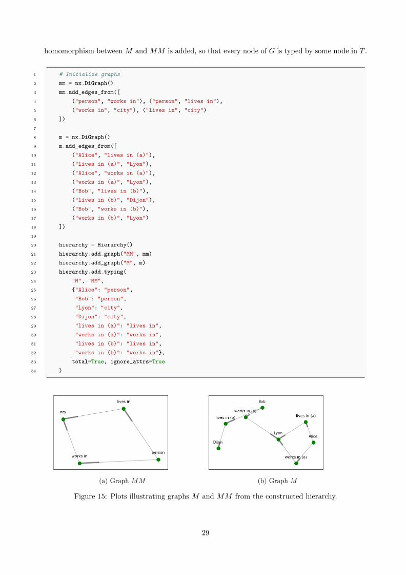
homomorphism between M and MM is added, so that every node of G is typed by some node in T .
1 # Initialize graphs
2 mm = nx.DiGraph()
3 mm.add_edges_from([
4 ("person", "works in"), ("person", "lives in"),
5 ("works in", "city"), ("lives in", "city")
6 ])
7
8 m = nx.DiGraph()
9 m.add_edges_from([
10 ("Alice", "lives in (a)"),
11 ("lives in (a)", "Lyon"),
12 ("Alice", "works in (a)"),
13 ("works in (a)", "Lyon"),
14 ("Bob", "lives in (b)"),
15 ("lives in (b)", "Dijon"),
16 ("Bob", "works in (b)"),
17 ("works in (b)", "Lyon")
18 ])
19
20 hierarchy = Hierarchy()
21 hierarchy.add_graph("MM", mm)
22 hierarchy.add_graph("M", m)
23 hierarchy.add_typing(
24 "M", "MM",
25 {"Alice": "person",
26 "Bob": "person",
27 "Lyon": "city",
28 "Dijon": "city",
29 "lives in (a)": "lives in",
30 "works in (a)": "works in",
31 "lives in (b)": "lives in",
32 "works in (b)": "works in"},
33 total=True, ignore_attrs=True
34 )
(a) Graph MM (b) Graph M
Figure 15: Plots illustrating graphs M and MM from the constructed hierarchy.
29

Type-respecting rewriting
Let us now define the following rewriting rule:
1 # Initialize the left-hand side
2 lhs = nx.DiGraph()
3 lhs.add_edges_from([(1, 2), (2, 3)])
4
5 # Initialize the preserved part
6 p = nx.DiGraph()
7 p.add_nodes_from([1, 2, 3])
8 p.add_edges_from([(1, 2)])
9
10 # Initialize the right-hand side
11 rhs = nx.DiGraph()
12 rhs.add_nodes_from([1, 2, 3, "Paris"])
13 rhs.add_edges_from([(1, 2), (2, "Paris")])
14
15 # By default if `p_lhs` and `p_rhs` are not provided
16 # to a rule, it tries to construct this homomorphisms
17 # automatically by matching the names. In this case we
18 # have defined lhs, p and rhs in such a way that that
19 # the names of the matching nodes correspond
20 rule_1 = Rule(p, lhs, rhs)
21
22 lhs_typing = {
23 "MM": {
24 1: "person",
25 2: "works in",
26 3: "city"
27 }
28 }
29 rhs_typing = {
30 "MM": {
31 "Paris": "city"
32 }
33 }
Figure 16: Rewriting rule defined in the previous listing (output ofregraph.plotting.plot rule)
30
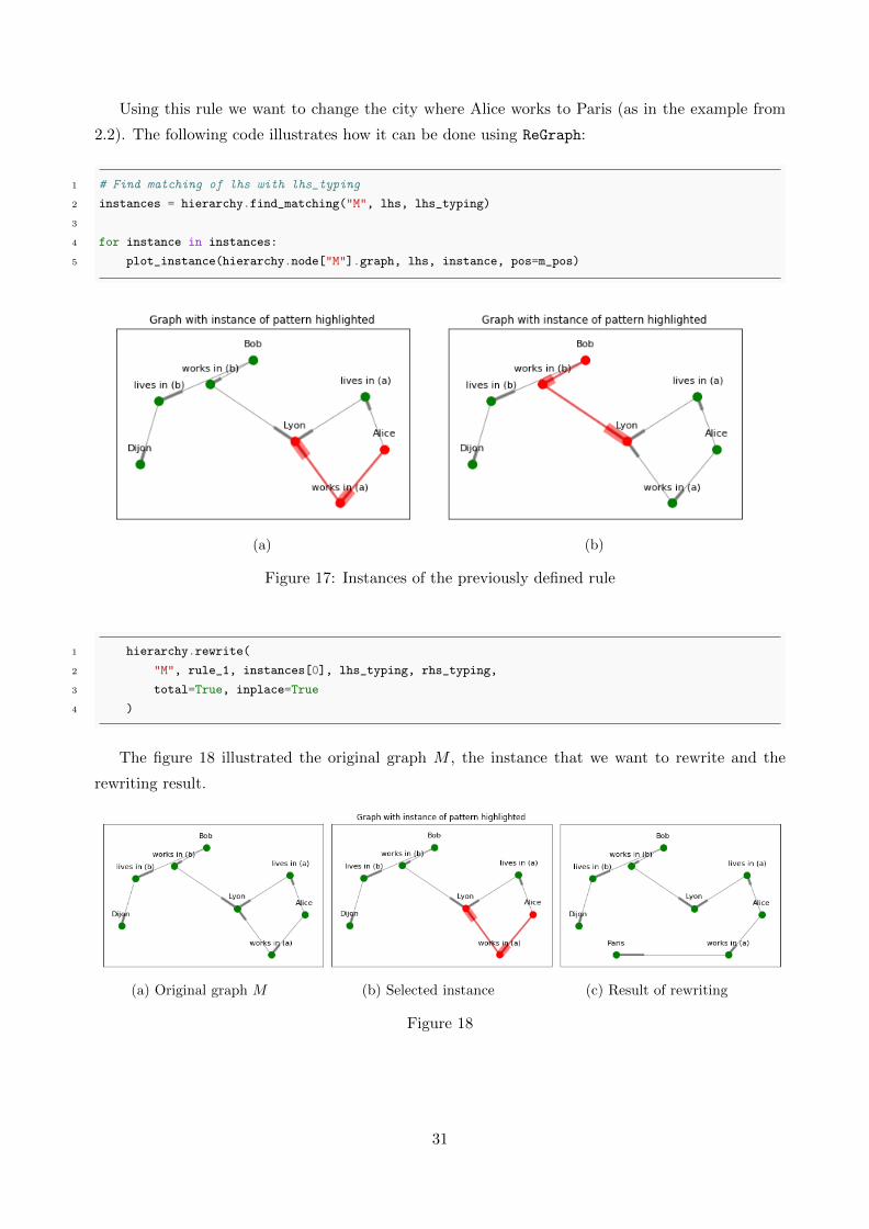
Using this rule we want to change the city where Alice works to Paris (as in the example from
2.2). The following code illustrates how it can be done using ReGraph:
1 # Find matching of lhs with lhs_typing
2 instances = hierarchy.find_matching("M", lhs, lhs_typing)
3
4 for instance in instances:
5 plot_instance(hierarchy.node["M"].graph, lhs, instance, pos=m_pos)
(a) (b)
Figure 17: Instances of the previously defined rule
1 hierarchy.rewrite(
2 "M", rule_1, instances[0], lhs_typing, rhs_typing,
3 total=True, inplace=True
4 )
The figure 18 illustrated the original graph M , the instance that we want to rewrite and the
rewriting result.
(a) Original graph M (b) Selected instance (c) Result of rewriting
Figure 18
31

Rewriting and propagation
Now consider another example of the meta-model rewriting and propagation of the changes to the
graph M . In the listing below we define a rule that clones the node ‘person’ in the meta-model and
creates two nodes ‘inhabitant’ and ‘employee’ connecting the first one to the node ‘lives in’ and the
second one to the node ‘works in’.
1 lhs = nx.DiGraph()
2 lhs.add_edges_from([("person", "lives in"), ("person", "works in")])
3
4 p = nx.DiGraph()
5 p.add_edges_from([("employee", "works in"), ("inhabitant", "lives in")])
6
7 # Right-hand side is identical to the preserved part
8 rhs = copy.deepcopy(p)
9 p_lhs = {
10 "employee": "person", "inhabitant": "person",
11 "works in": "works in", "lives in": "lives in",
12 }
13
14 rule_2 = Rule(p, lhs, rhs, p_lhs)
Figure 19: Rewriting rule defined in the previous listing (output ofregraph.plotting.plot rule)
Similarly, we search for the matching of the left-hand side of the rule in the graph MM and with
the selected instance we rewrite MM in the hierarchy.
1 instances = hierarchy.find_matching("MM", lhs)
2 hierarchy.rewrite("MM", rule_2, instances[0], total=True, inplace=True)
(a) Original graph MM (b) Selected instance (c) Result of rewriting
32

As the result of rewriting of MM in the hierarchy graph the respective changes are propagated
to M :
Figure 21: M after propagation of changes in MM
The following code:
1 print("Alice - type: ", hierarchy.node_type("M", "Alice")["MM"])
2 print("Alice1 - type: ", hierarchy.node_type("M", "Alice1")["MM"])
3 print("Bob - type: ", hierarchy.node_type("M", "Bob")["MM"])
4 print("Bob1 - type: ", hierarchy.node_type("M", "Bob1")["MM"])
outputs:
Alice - type: inhabitant
Alice1 - type: employee
Bob - type: inhabitant
Bob1 - type: employee
33
Appendix E Example of programmatic KAMI usage
The following listing contains an example of usage of KAMI API for programmatic input of inter-
actions to the hierarchy.
1 from kami.data_structures.entities import (Agent, Region,
2 PhysicalAgent,
3 Residue, State,
4 PhysicalRegion,
5 PhysicalRegionAgent)
6 from kami.data_structures.interactions import Modification
7 from kami.resolvers.black_box import create_nuggets
8
9 # Initialize an empty hierarchy
10 hierarchy = KamiHierarchy()
11
12 # Define interactions
13 mek1 = PhysicalAgent(Agent("Q02750"))
14 stat3 = PhysicalAgent(Agent("P40763"))
15 mod_state_1 = Residue("S", 727, State("phosphorylation", False))
16 mod1 = Modification(mek1, stat3, mod_state_1, value=True, direct=True)
17
18 mod_state_2 = Residue("Y", 705, State("phosphorylation", False))
19 mod2 = Modification(mek1, stat3, mod_state_2, value=True, direct=True)
20
21 erk1 = PhysicalAgent(Agent("P27361"))
22 mod_state_3 = Residue("T", 201, State("phosphorylation", False))
23 mod3 = Modification(mek1, erk1, mod_state_3, value=True, direct=True)
24
25 erk2 = PhysicalAgent(Agent("P28482"))
26 mod_state_4 = Residue("T", 182, State("phosphorylation", False))
27 mod4 = Modification(mek1, erk2, mod_state_4, value=True, direct=True)
28
29 interactions = [mod1, mod2, mod3, mod4]
30
31 # Create nuggets from the interactions
32 create_nuggets(
33 interactions,
34 hierarchy,
35 add_agents=True,
36 anatomize=True
37 )
In this example genes (instances of kami.data structures.entities.Agent) are defined by
their UniProt accession number. The resolver module of KAMI creates nuggets corresponding to
these interactions. Moreover, using the agent anatomizer it adds new nodes corresponding to the
genes in the action graph together with their domains. The resolver also identifies that all the
interactions are phosphorylations and that the enzyme (with identifier Q02750) contains a protein
kinase domain, therefore all the modification nodes in the nuggets are mapped to a single modification
34

action in the action graph, which represents the addition of phosphate group to the substrate by the
protein kinase domain. The following figure illustrates the resulting nuggets and the corresponding
action graph:
mod
phospho
res S727
STAT3
68-361
MEK1
mod
phospho
res Y705
STAT3
68-361
MEK1
mod
phospho
res T201
ERK1
68-361
MEK1
mod
phospho
res T182
ERK2
68-361
MEK1
(a)
68-361 (Pk) MEK1 mod1
584-674
STAT3
141-319
321-573
2-119
res 727
phospho
phospho
phospho
phospho
res 705
42-330 (Pk)
ERK1
res 201
25-313 (Pk)
ERK2res 182
(b)
Figure 22: Visualization of (a) the nuggets and (b) the action graph produced in the listing(plotted with Gephi). Regions are represented with the nodes containing integer intervals, wealso denote with ‘(Pk)’ protein kinase domains.
35
Related Documents