Welcome message from author
This document is posted to help you gain knowledge. Please leave a comment to let me know what you think about it! Share it to your friends and learn new things together.
Transcript

UNIVERSIDADE FEDERAL FLUMINENSE
SANDERSON LINCOHN GONZAGA DE OLIVEIRA
Graph-based adaptive simplicial-mesh renement fornite volume discretizations
Niterói
2009
UNIVERSIDADE FEDERAL FLUMINENSE
SANDERSON LINCOHN GONZAGA DE OLIVEIRA
Graph-based adaptive simplicial-mesh renement fornite volume discretizations
Thesis submitted to the Programa de Pós-
Graduação em Computação at Universidade
Federal Fluminense in partial fullllment of
the requirements for the degree of Doctor in
Computer Science.
Advisor:Mauricio Kischinhevsky
Niterói
2009
Graph-based adaptive simplicial-mesh renement fornite volume discretizations
SANDERSON LINCOHN GONZAGA DE OLIVEIRA
Tese submetida ao Programa de Pós-Graduação emComputação da Universidade Federal Fluminense comorequisito parcial para obtenção de título de Doutor.Área de concentração: Modelagem Computacional.
Aprovada por:
Prof. D.Sc. Mauricio Kischinhevsky / IC-UFF (Presidente)
Prof. Ph.D. Jorge Stol / IC-UNICAMP
Prof. Ph.D. Carlos Antonio de Moura / IME-UERJ
Prof. D.Sc. Luiz Nélio Henderson Guedes de Oliveira / IPRJ-UERJ
Profa. D.Sc. Regina Célia Paula Leal Toledo / IC-UFF
Profa. D.Sc. José Henrique Carneiro de Araújo / IC-UFF
Prof. D.Sc. Anselmo Antunes Montenegro / IC-UFF
Niterói, 26 de janeiro de 2009.
Este trabalho é dedicado
a meu pai,
Luiz Gonzaga de Oliveira,
à doce Tatiana Maduro
e
à memória de minha mãe,
Selma Andrade de Oliveira.
Acknowledgements
I must express my gratitute to many people who helped me during this work. Trying to
mention all of them would certainly lead me to an incomplete list with someone important
missing. However, I am particularly grateful to Professor Mauricio Kischinhevsky for his
supervision and teaching and to Tatiana Barbosa Maduro, Jacques Alves da Silva, Diego
Nunes Brandão and Mauricio José Guedes for their contributions. Likewise, I acknowledge
CAPES for the nancial support. Similarly, I thank the entire group of professors and
employees from IC-UFF. I also must express my thanks to Prof. Denise Burgarelli for
sending me the program code to solve the Laplace Equation based on the quadrangular
ALG.
Abstract
This work proposes an adaptive mesh renement technique for discretizations based on
triangles of any shape. It employs the Finite Volume Method in a cell-centered scheme
in order to solve partial dierential equations. The mesh is represented by a graph data
structure. The scheme intends to reduce the computational cost to construct the rened
mesh in evolutionary problems. Furthermore, it admits more exibility to link nodes
among neighbors in dierent levels of renement, in comparison to a local renement
scheme which uses a tree-like data structure. A Sierpi«ski-like Curve is used to order
the nite volumes. Volumes are rened by the 4-triangles longest-side partition scheme,
allowing straightforward updating of the linked list. A specic linear approximation is
used to determine the gradients of diusive and viscous terms and the dependent variable
of the partial dierential equation in the control volume is solved by a specic linear inter-
polation. Additionally, linear-system solvers based on the minimization of functionals can
be easily employed. Specically, the Conjugate Gradient Method is used. This approach
enables any polygonal shape in the initial domain. Numerical results demonstrate the
eciency and advantages of this scheme.

Keywords
1. Numerical methods
2. Numerical solution and simulation of PDEs
3. Finite Volume Method
4. Adaptive mesh renement
5. Computational analysis
6. Space-lling curve
7. Sierpi«ski Curve
8. Eulerian approach
9. Eulerian-Lagrangian approach

Glossary
2D : two-dimensional;
3D : three-dimensional;
4TLSP : 4-triangles longest-side partition;
ALG : Autonomous Leaves Graph;
AMR : adaptive mesh renement;
FVM : Finite Volume Method;
M : mass inside a volume;
PDE : Partial Dierential Equation;
R : reference length used in the Reynolds number;
S : source term;
p : pressure;
t : time;
~u : velocity vector;
u∞ : air velocity in the free-stream region (at-plate Boundary Layer Problem);~A : vector area;
ν : kinematic viscosity;
φ : density of a substance;
ρ : specic uid mass;
Γφ : diusive coecient;
4 : velocity boundary-layer thickness (at-plate Boundary Layer Problem).

Contents
List of Figures x
1 Introduction 1
1.1 Uniform meshes × AMR technique . . . . . . . . . . . . . . . . . . . . . . 2
1.2 Tree-like × graph-based data structures . . . . . . . . . . . . . . . . . . . . 3
1.3 Triangular meshes . . . . . . . . . . . . . . . . . . . . . . . . . . . . . . . . 4
1.4 A graph-based adaptive triangular mesh renement for nite volume ap-proximations . . . . . . . . . . . . . . . . . . . . . . . . . . . . . . . . . . 4
1.5 Brief introduction to the Finite Volume Method . . . . . . . . . . . . . . . 5
1.5.1 Convergence analysis . . . . . . . . . . . . . . . . . . . . . . . . . . 6
2 A review of nite volume schemes with triangular meshes 7
2.1 A brief comparison between cell and vertex-centered control volume schemes 7
2.2 A review of vertex-centered control volume schemes . . . . . . . . . . . . . 8
2.2.1 The Median dual scheme . . . . . . . . . . . . . . . . . . . . . . . . 8
2.2.2 Voronoi Diagrams . . . . . . . . . . . . . . . . . . . . . . . . . . . . 10
2.3 A review of cell-centered control volume schemes . . . . . . . . . . . . . . . 11
2.3.1 Cell-centered Green-Gauss integration technique . . . . . . . . . . . 12
2.3.2 Cell-centered least-squares schemes . . . . . . . . . . . . . . . . . . 12
2.3.3 The Green-Gauss technique and the least-squares method . . . . . . 12
2.4 A review of higher-order resolution schemes . . . . . . . . . . . . . . . . . 13
2.4.1 MUSCL . . . . . . . . . . . . . . . . . . . . . . . . . . . . . . . . . 14
2.4.2 PPM . . . . . . . . . . . . . . . . . . . . . . . . . . . . . . . . . . . 14
2.4.3 ENO . . . . . . . . . . . . . . . . . . . . . . . . . . . . . . . . . . . 14

Contents viii
2.4.4 WENO . . . . . . . . . . . . . . . . . . . . . . . . . . . . . . . . . . 14
2.4.5 Quadratic reconstruction . . . . . . . . . . . . . . . . . . . . . . . . 15
2.4.6 H -box methods . . . . . . . . . . . . . . . . . . . . . . . . . . . . . 15
2.4.7 Frinck's reconstruction . . . . . . . . . . . . . . . . . . . . . . . . . 16
2.4.8 CIP . . . . . . . . . . . . . . . . . . . . . . . . . . . . . . . . . . . 16
2.4.9 CIVA . . . . . . . . . . . . . . . . . . . . . . . . . . . . . . . . . . 16
2.4.10 ADER . . . . . . . . . . . . . . . . . . . . . . . . . . . . . . . . . . 17
2.4.11 Other schemes . . . . . . . . . . . . . . . . . . . . . . . . . . . . . . 17
3 Description of a discrete formulation based on the Finite Volume Method 18
3.1 A nite volume approximation . . . . . . . . . . . . . . . . . . . . . . . . . 19
3.1.1 Linear interpolation of the convective term . . . . . . . . . . . . . . 21
3.1.2 Treatment of the diusion term . . . . . . . . . . . . . . . . . . . . 23
4 A graph-based adaptive mesh renement technique with triangular cell-centeredvolumes 26
4.1 The 4-triangles longest-side partition of volumes . . . . . . . . . . . . . . . 27
4.1.1 The 4-triangles longest-side partition scheme . . . . . . . . . . . . . 27
4.2 A graph-based AMR representation of triangular cell-centered volumes . . 29
4.3 Graph simplication for volumes of the same level . . . . . . . . . . . . . . 31
4.4 Generalization of the renement scheme . . . . . . . . . . . . . . . . . . . 31
4.5 Unrenement process . . . . . . . . . . . . . . . . . . . . . . . . . . . . . . 33
5 Mesh total ordering 36
5.1 Sierpi«ski Curve . . . . . . . . . . . . . . . . . . . . . . . . . . . . . . . . . 37
5.2 Sierpi«ski-like Curve for the total-order relation on the triangular volumesof the mesh . . . . . . . . . . . . . . . . . . . . . . . . . . . . . . . . . . . 39
6 Experimental tests 40
6.1 Information system modeling using UML . . . . . . . . . . . . . . . . . . . 40

Contents ix
6.2 Renement criteria . . . . . . . . . . . . . . . . . . . . . . . . . . . . . . . 41
6.3 Laplace Equation (elliptic problem) . . . . . . . . . . . . . . . . . . . . . . 42
6.4 Heat Conduction Equation (parabolic problem) . . . . . . . . . . . . . . . 43
6.4.1 Performance of the renement process . . . . . . . . . . . . . . . . 43
6.4.1.1 Complexity analysis of the space-lling curves: MHC andSierpi«ski-like Curve . . . . . . . . . . . . . . . . . . . . . 47
6.4.1.2 Quadrangular volumes× Triangular volumes . . . . . . . 52
6.5 Wave Equation (hyperbolic problem) . . . . . . . . . . . . . . . . . . . . . 52
6.6 Flat-plate Boundary Layer Problem . . . . . . . . . . . . . . . . . . . . . . 55
6.6.1 A nite volume discretization of the Boundary Layer Problem . . . 56
6.6.2 The analytical solution of the at-plate Boundary Layer Problem . 57
6.6.3 A numerical simulation of the at-plate Boundary Layer Problem . 58
7 Conclusion 61
Appendix A -- Some historical descriptions 63
Appendix B -- Finite volume approximations 69
Appendix C -- A mathematical proof by induction 71
Appendix D -- Remarks for 3D 76
Bibliography 78

List of Figures
2.1 Triangulation duals. . . . . . . . . . . . . . . . . . . . . . . . . . . . . . . . 8
2.2 (a) A control volume of the Median dual scheme and; (b) a control volumefrom the scheme proposed by [Schneider and Raw, 1987]. . . . . . . . . . . 9
2.3 A Voronoi volume. . . . . . . . . . . . . . . . . . . . . . . . . . . . . . . . 10
2.4 Example meshes with control volumes in the proper nite volume. . . . . . 11
3.1 Three neighbor volumes, whose centroids areP, 1 and 2, whereas ip is theintegration point between volumesP and 1. . . . . . . . . . . . . . . . . . 20
4.1 (a) Renement by simple centroid insertion; (b) Renement by centroidinsertion and adding midpoints of the three edges; (c) Renement by addingthe three midpoints; and (d) Renement by successive bisections. . . . . . 27
4.2 A triangular volume rened, the single graph node that represented theoriginal triangular volume and on the mostright side a sub-graph createdafter a renement of the triangular volume, respectively. The opposite isperformed in the unrenement process. . . . . . . . . . . . . . . . . . . . . 30
4.3 Unit square as the problem domain; and links of the graph data structure- nodes represent the renement of level 0. . . . . . . . . . . . . . . . . . . 30
4.4 Renement example with triangular volumes; and graph with transitionand volume nodes that forms the scheme of this triangular volume rene-ment, respectively. . . . . . . . . . . . . . . . . . . . . . . . . . . . . . . . 31
4.5 Renement of another volume depicted in Fig. 4.4, its graph representa-tion, and graph simplication, respectively. . . . . . . . . . . . . . . . . . . 31
4.6 Volume rened directly in sixteen new volumes, and its graph representa-tion, respectively. . . . . . . . . . . . . . . . . . . . . . . . . . . . . . . . . 33
4.7 A discretized domain and its graph representation showing a pack selectedto be unrened. . . . . . . . . . . . . . . . . . . . . . . . . . . . . . . . . . 34
4.8 Final conguration of the discretization, pack collapse, and nal congu-ration of the graph, respectively. . . . . . . . . . . . . . . . . . . . . . . . . 34
List of Figures xi
5.1 Generator process of the Sierpi«ski Curve through equilateral triangles di-vided into 4, 10 and 22 triangles, respectively. . . . . . . . . . . . . . . . . 37
5.2 Sierpi«ski Curve generation. . . . . . . . . . . . . . . . . . . . . . . . . . . 37
5.3 Sierpi«ski Curve ordering scalene triangles. . . . . . . . . . . . . . . . . . . 37
5.4 Sierpi«ski Curves in a unit square with 23, 23, . . ., 211 volumes. . . . . . . . 38
5.5 Successive adaptive renements with volumes ordered by a Sierpi«ski-likeCurve on the right-hand side of each discretization. . . . . . . . . . . . . . 39
6.1 Simplied diagram class of this work. . . . . . . . . . . . . . . . . . . . . . 41
6.2 Sierpinski-like Curve of the AMR scheme applied to the Laplace Equation. 42
6.3 Final mesh conguration of an AMR approximation to the Heat Conduc-tion Equation. . . . . . . . . . . . . . . . . . . . . . . . . . . . . . . . . . . 44
6.4 Final time step of an AMR approximation to the Heat Conduction Equa-tion with boundary condition: x− y. . . . . . . . . . . . . . . . . . . . . . 44
6.5 AMR approximation of the Heat Conduction Equation with boundary con-dition: x2 − y2. . . . . . . . . . . . . . . . . . . . . . . . . . . . . . . . . . 45
6.6 Volume ordering in a local triangular renement. . . . . . . . . . . . . . . 48
6.7 AMR approximation of the Wave Equation through the Modied Methodof Characteristics. . . . . . . . . . . . . . . . . . . . . . . . . . . . . . . . . 55
6.8 Flat-plate boundary-layer process. . . . . . . . . . . . . . . . . . . . . . . . 56
6.9 Flat-plate boundary-layer process forφ = 10m/s. . . . . . . . . . . . . . . 58
6.10 Flat-plate Boundary Layer Problem withu∞ = 10, ν = 1.5 · · · 10−5, u∞ =
10, and (x, y) = [0; 1]2. . . . . . . . . . . . . . . . . . . . . . . . . . . . . . 59
6.11 Error of the numerical approximations to the at-plate Boundary LayerProblem with u∞ = 10, ν = 1.5 · · · 10−5, u∞ = 10, and (x, y) = [0; 1]2. . . . 60
B.1 Elementar 2D control volume. . . . . . . . . . . . . . . . . . . . . . . . . . 70
D.1 (a) Tetrahedral volume with view from top; (b) detail of the front faceview; (c) detail of the left front face view; (d) detail of the background faceand; (e) detail of the right face. . . . . . . . . . . . . . . . . . . . . . . . . 76
D.2 (a) original tetrahedral; (b) new tetrahedral, which is in the back; (c) newtetrahedral, which is in front; (d) both new tetrahedral uncoupled; (e) fournew tetrahedral; (f) rst two tetrahedra and (g) last two tetrahedra. . . . . 77
List of Figures xii
D.3 (a) Three tetrahedral volumes (GFBC, FACB and CBAD); (b) renementof the front left tetrahedral volume into two new ones where black pointsindicate the tetrahedral volume centroids and there is a curve representingthe 3D Sierpi«ski-like Curve as well as lines indicating median lines of thebackground of tetrahedral volumes. . . . . . . . . . . . . . . . . . . . . . . 77
Chapter 1
Introduction
The Finite Volume Method is a numerical method for solution of partial dierential equa-tions (PDEs). It is a method for representing and evaluating PDEs as algebraic1 equationsand values are calculated at discrete places on a meshed geometry. This results in a linearsystem to be computed. When one increases the number of discrete places in the dis-cretized domain in order to improve the quality of the numerical solution, the resultinglinear system is proporcionally increased. As a result, the computational cost in order tocompute the resulting linear system is also increased. On the other hand, the solutionmay require more discrete places only where the solution and/or its derivatives changerapidly. Thus, the adaptive mesh renement (AMR) technique is used to concentratemore discrete places in certain regions of the mesh allowing a coarse level of renementin other regions. Increasing discrete places only in such regions of the discretized domainpresents two characteristics: i) allows to maintain the quality being sought and; ii) theresulting linear system is smaller than a solution in which the discretized domain is uni-formly rened. For evolutionary problems, such scheme becomes particularly importantsince, by the dynamic nature of such problems, migration (or occurrence) of regions ofrapid solution change may happen whereas the solution in other parts is relatively stable.Thus, a non-uniform (irregular or sometimes used as unstructured in the nite volumeeld) mesh is adaptively rened in order to improve the quality of a computed solution.
1Appendix A presents historical descriptions of some terms, researchers, and others.

1.1 Uniform meshes × AMR technique 2
1.1 Uniform meshes × AMR technique
In relation to data structures, a mesh of a numerical method should eciently describethose features. A mesh is called uniform if each discrete place has the same numberof neighbors. In terms of data structures, it requires to deal with discrete places justthrough indices of multi-dimensional arrays and matrices. Using a regular mesh in orderto cover the domain of the dierential problem is not appropriate in certain situationsbecause those meshes do not take into account the dierent scales of the phenomena beingstudied. Usually, regular meshes are computationally expensive because they should havea large number of discrete places in the entire discretized domain in order to provide aquality solution.
On the other hand, techniques that use AMR are, usually, computationally less ex-pensive in certain problems than using a uniform mesh. In other words, an AMR schemecan signicantly improve the computational eciency of scientic and engineering calcu-lations involving solutions to large gradients, complicated geometries, and other specialcharacteristics in problems. Emphasizing, the idea is to automatically build a coarsemesh whose numerical solution provides an appropriate approximation and to constructa ne mesh where the numerical solution does not supply an appropriate approximationamong cells, such as singularities, boundary layers, among others. Furthermore, it shouldhave a smooth transition among neighbor discrete places, which have dierent levels ofrenement. Usually, an AMR reduces the required number of discrete places to obtainan accurate numerical solution to problems that are almost smooth, and can reach anumerical solution with the desired quality in non-smooth problems.
[Rivara, 1984a] explained that multigrid methods use iterative solvers of equations tosmooth either the solution or related residual functions over ne and coarse grids. Thisproceeds only until the functions become smooth, namely, while the iterative methods arerapidly convergent. Adaptivity of the mesh is a central feature since it relieves the user ofcritical decisions and allows use of all the exibility of the a numerical method for gettinga minimum number of discrete places. In this sense, the generation of the discretization(triangulation) should not be a rst separate step of the solution process, but a dynamicadaptive process. In order to deal with singular solutions, the capability for managinglocal renement of the discretization is indispensable, and mesh renement algorithmsthat maintain the nondegeneracy of the volumes and smoothness of the mesh are certainlydesirable. The techniques chosen to satisfy the dierent goals proposed should also ttogether in an ecient way. One of the most critical decisions with this kind of softwareis the denition of data structure to be used to construct the sequence of discretizedproblems and to manage the multigrid method. This denition must necessarily considerthe dierent algorithms to be used with it.
1.2 Tree-like × graph-based data structures 3
1.2 Tree-like × graph-based data structures
Usually, a tree-like data structure is used in order to construct regions of the mesh withmore discrete places. From an initial discretization, represented by the root of a tree-like data strucutre, children nodes are created recursively, which represent the discretizeddomain with more discrete places. When setting up the linear system, connectivity in-formation among neighbors is needed. Using a tree-like data structutre, this can be onlyobtained from a leaf node li seeking (up) many nodes until a certain original node in com-mon (also one original node of the leaf node being searched) and again seeking (down)the leaf node lj that is the neighbor of the leaf li.
In order to avoid this overhead, [Burgarelli, Kischinhevsky and Biezuner, 2006] pro-posed a graph-based data structure for representing the AMR. In this work, either neigh-bors can be directly connected or the steps to reach nodes among neighbors are greatlyreduced when there are dierent levels of renement among cells. The authors pro-posed a simple, yet exible and powerful, strategy within a group of methods thatdeal with the AMR scheme, which provides local mesh renement with low compu-tational cost. The technique displays a plug-in feature that enables replacement ofa single discrete place by a pack of discrete places in any region of interest. More-over, only strict local changes in the data structure occur. Besides, low storage isachieved since the rened nodes are not stored. The authors named the graph datastructure as Autonomous Leaves Graph (ALG). ALG represents a mesh composed bysquare-shaped control volumes and the initial discrete domain is, generally, a unit square.In [Brandao, Gonzaga and Kischinhevsky, 2008], the scheme was applied with square-shaped nite-element approximations in the Laplace Equation Problem and, similarly,in [Brandao, Gonzaga and Kischinhevsky, 2009], it was applied in the Poisson EquationProblem. Furthermore, as long as a discrete place is rened, a graph node is substitutedby a sub-graph that represents the new discrete places inserted. The data structure wasespecially designed to minimize the number of operations needed in the AMR process.Implementation of this AMR scheme allows exibility in reaching neighbors with dier-ent levels of renement. Since ALG was not conceived with any particular problem orgeometry, its concepts can be applied to the study of several phenomena and classes ofPDEs. To summarize, there are low storage requirements and low computational costwhen representing an AMR.

1.3 Triangular meshes 4
1.3 Triangular meshes
Triangular meshes, or triangulations, are one of the most widely used representations forgeometric models. A triangulation is a 2D simplicial complex, a simple structure with con-venient combinatorial properties [Velho, Figueiredo and Gomes, 1999]. Simplicial meshescan be related to general meshes. Here, the meshes are related to simplicial complexstructures (see [Velho, Figueiredo and Gomes, 1999]) in non-conform meshes since thoseare not a concern in nite volume discretizations.
A triangular mesh is said to be distorted (or bad quality) if it has triangles in whichthe ratio between the radius r of the incircle and the radius R of the cincumcircle of thetriangle tends to zero ( r
R<< 1). Thus, generating a quality mesh is crucial when solving
PDEs. This present work intends to generate quality meshes during the dynamic AMRprocess.
1.4 A graph-based adaptive triangular mesh renementfor nite volume approximations
Considering those aspects, this work follows the concepts of the graph data structure pro-posed by [Burgarelli, Kischinhevsky and Biezuner, 2006]; however, in this present work,the graph data structure represents a triangular mesh. Thus, the main novelty proposedhere is that this technique uses a discrete adaptive mesh comprised of volumes with anytriangular shape and the mesh is represented by a graph. An irregular mesh comprised oftriangular volumes can be more appropriate near physical boundary regions and featuresof a problem with complex geometries. In relation to the total ordering, a Hamiltoniantriangulation is generated with respect to the Hamiltonian ordering found. Additionally,linear-system solvers based on the minimization of functionals can be easily employed.Moreover, this technique operates all the required elements for AMR in the Finite Vol-ume Method. Triangular meshes are shown in the experimental tests in order to exemplifythis technique.
1.5 Brief introduction to the Finite Volume Method 5
1.5 Brief introduction to the Finite Volume Method
The Finite Volume Method (FVM) has been applied to approximate complex problems inseveral areas of science and engineering, especially for environmental draining, predictionof scattering of pollutants in the atmosphere, water and earth, in aerodynamic problems,draining study over several surfaces, in petroleum reservoirs, in simulations to increaseeciency of recovery of petroleum in a reservoir, among others.
As stated before, the FVM is a method for representing and evaluating PDEs asalgebraic equations and values are calculated at discrete places on a meshed geometry.Finite volume refers to the small volume surrounding each node point on a mesh. Inthe FVM, volume integrals in a PDE that contain a divergence term are converted tosurface integrals using the Divergence Theorem [Leithold, 1994]. In Vector Calculus, theDivergence Theorem, also known as Gauss Theorem or Ostrogradsky-Gauss Theorem, isa result that links the divergence of a vector eld to the value of surface integrals of theow dened by the eld. Those terms are then evaluated as uxes at the surfaces ofeach nite volume. Because the ux entering a given volume is identical to that leavingthe adjacent volume, these methods are conservative. Another advantage of the FVM isthat it is easily formulated to allow unstructured meshes. The method is used in manycomputational uid dynamics packages [Versteeg and Malalasekera, 1995].
In other words, the FVM is naturally based on the mass conservation laws and itsapplication is simple and convenient. Classically, it is applied to a PDE in its conservativeform, that is, with conservation laws. Such equations characteristically employ a divergentoperator. Each equation is located in each control volume and the Divergence Theoremconverts each equation to the integral of the ux along the boundary of the control volume.Moreover, integral conservation laws state that the total size rate of a substance withdensity φ in a specic nite volume is equal to the total ux of the substance through thenite volume boundary. Namely, the key concept used during the FVM formulation is theprinciple of conservation of a specic physical quantity expressed by governing equationsover any nite volume.
The mesh generation with a proper generation of control volumes is required. Thisshould be carefully considered in order to obtain an optimal order of convergence. Theaverage ux along each edge of a control volume is then approximated by a special nite-dierence scheme by using data in the neighboring cells. From the code implementationpoint of view, FVM is easier to code than other similar numerical methods. Appendix Bpresents a brief introduction to nite volume approximations by integrating the PDE inthe conservative form on an elementar control volume.
To summarize, the ux domain is discretized in a set of non-overlapped control vol-

1.5 Brief introduction to the Finite Volume Method 6
umes, which can be irregular in size and shape. Namely, similarly to other methods thatobtain approximated equations from balance equations, the FVM consists of integratingthe dierential equation in a conservative form of the control volume set.
1.5.1 Convergence analysis
The reader is referred to [Arnold, 2001] for an introduction to numerical analysis. Basi-cally, convergence analysis of the Finite Volume Method can be obtained from the frame-work of the Finite Element Method (FEM). Indeed, convergence can be analyzed directlyin discrete norms, or function space norms can be used by constructing either an equivalentor an asymptotically equivalent FEM. Some authors obtained stability and convergenceanalysis from other forms, which do not use a FEM basis [Jeon and Sheen, 2005]. Forexample, [Bouche, Ghidaglia and Pascal, 2005] investigated the order of convergence ofthe upwind FVM for solving linear steady convection problem on a bounded domain withnatural boundary conditions. In order to overcome the non-consistency in the nite dier-ence sense of the scheme, those authors introduced a sequence that they called geometriccorrectors. It is associated with each nite volume and each constant convection vector.Under a local quasi-uniformity condition for the triangulation and if the continuous solu-tion is regular enough, they rst established a link between the convergence of the nitevolume scheme and those geometric correctors. As a result, the study of that correctorin the case of uniformly rened triangular meshes in 2D led to the proof of the optimalorder of convergence for the nite volume scheme.
After this brief introduction, Chapter 2 deals with the discretization schemes used inthe FVM with irregular meshes. Chapter 3 presents the numerical solution adopted. Al-though informally presented, the algebraic operations in Chapter 3 are somewhat technicaland may be omitted on a rst reading. Chapter 4 explains the 4-triangles longest-sidepartition of triangular volumes, and also introduces the AMR scheme as well as discussesthe graph data structure in detail, including the renement/unrenement process. Sincethe characterists in Chapter 4 are the main novelties proposed, it can be considered asthe core of this work. Another important feature of this work is presented in Chapter 5.It briey explains the space-lling curve employed to number the mesh nodes and givesdetails of the mesh total ordering. Chapter 6 discusses the experimental tests. Finally,Chapter 7 discusses some additional remarks and presents future directions as well.

Chapter 2
A review of nite volume schemes withtriangular meshes
Approaches seek appropriate forms in order to fulll the Finite Volume Method (FVM)requirements, e.g. to adequately establish an orthogonal segment between evaluationpoints and the outward normal vector, which is used in the Divergence Theorem.
Generally, there are two main schemes for nite volume discretizations in triangularmeshes: cell-centered and vertex-centered. Both discretizations dier in the location ofthe control volumes in the mesh and the ux variable:
(i) In cell-centered schemes, ux quantities are stored in the nite volume centroidthemselves and the mesh has simple geometry;
(ii) In vertex-centered schemes, ux variables are stored in the mesh vertices. Conse-quently, control volumes are comprised of sub-nite volumes, i.e. parts of nite volumes,which the vertex belongs.
2.1 A brief comparison between cell and vertex-centeredcontrol volume schemes
Vertex-centered schemes are rst-order accurate on distorted grids. On Cartesian or onsmooth grids, the vertex-centered schemes are second or higher-order accurate dependingon the ux evaluation scheme. On the other hand, the discretization error of cell-centeredschemes depends strongly on the smoothness of the grid. In general, a cell-centered schemeon triangular/tetrahedral grid leads to about two/six times more control volumes than avertex-centered scheme. Hence, cell-centered schemes have more degrees (more unknowns)of freedom than the Median dual scheme (see 2.2.1). In addition, control volumes in cell-centered schemes are usually smaller than those in vertex-centered schemes. This suggests

2.2 A review of vertex-centered control volume schemes 8
Figure 2.1: Triangulation duals.
that cell-centered schemes are more accurate than vertex-centered schemes. However,residual of cell-centered schemes results from much smaller number of uxes compared tothe Median dual scheme, which is a vertex-centered scheme (see Section 2.2.1). Boundarycondition implementation in vertex-centered schemes requires additional logic in order toassure a consistent solution at boundary points, contrary to cell-centered schemes, whichis simple [Yousuf, 2005]. As a result, there is no clear evidence about the better scheme.
There are publications that used both cell and vertex-centered strategies. Amongthese examples one nds [McManus et al., 2000], who showed a scalable strategy for theparallelization of multiphysics unstructured mesh-iterative codes on distributed-memorysystems.
2.2 A review of vertex-centered control volume schemes
In general, there are two main triangular vertex-centered schemes: the Median dualscheme for general triangular meshes and Voronoi Diagrams (or the Dirichlet tessela-tion). Both create a dual mesh for determining the required quantities. In Fig. 2.1 (from[Barth, 1994]), edges and faces around the central vertex are formed by duals mediansegments, centroid segments, and by the Dirichlet Tesselation.
2.2.1 The Median dual scheme
One of the rst formulations using triangular meshes for the generation of control vol-umes appeared in the end of 1970s and in the begining of 1980s, proposed by Baliga andPatankar [Schneider and Maliska, 2002]. The Finite Element Method (FEM) test func-tions were adapted to the nite-volume discretization. Figure 2.2a (from[Schneider and Maliska, 2002]) depicts a control volume according to this scheme.

2.2 A review of vertex-centered control volume schemes 9
Figure 2.2: (a) A control volume of the Median dual scheme and; (b) a control volumefrom the scheme proposed by [Schneider and Raw, 1987].
The Median dual scheme can be used with general meshes. It plays a special rolebecause one can show that using a specic numerical quadrature, the FEM method withlinear elements and the FVM on median duals are equivalent [Barth and Ohlberger, 2004].This enables convergence analysis directly from the FEM.
Although the Median dual scheme enables generic mesh usage, consider a DelaunayTesselation (or triangulation), common in the FEM, where the control volumes are gen-erated, depicted in Fig. 2.2a. The geometric center of the triangle P12 in Fig. 2.2a isjoined to the mean point of its edges P1 and P2. Thus, the ve triangular elements, sim-ilar to the element P12, form the control volume centered in P. Each triangular elementcontributes with two integration points, ip1 and ip2, in the balance conservation of thecontrol volume centered in P.
Aiming towards maintaining the praticity in the mesh generation,[Schneider and Raw, 1987] proposed to obtain control volumes similarly to the proposalin [Baliga and Patankar, 1980]. Their approach is based on a mesh formed by quadranglessimilarly to the generalized coordinates [Schneider and Maliska, 2002]. The advance in theeld given in [Schneider and Raw, 1987] was the coupling introduced in the equations inorder to improve the convergence process. Figure 2.2b (from [Schneider and Maliska, 2002])illustrates an elementar volume according to this scheme. The control volumes are ob-tained by joining the barycenter of the quadrangle P123 to the mean point of the edges.Quadrangular elements similar to the element P123 form the control volume centered inP. Furthermore, a local coordinate system is needed in order to implement the approxi-mations. It provides more options to create the mesh and does not need to have a xednumber of points in the coordinate directions, what diers from the generalized coordi-nates [Schneider and Maliska, 2002]. Each element also contributes with two integrationpoints, ip and ip1, in the balance conservation of the control volume centered in P.

2.2 A review of vertex-centered control volume schemes 10
Figure 2.3: A Voronoi volume.
2.2.2 Voronoi Diagrams
Voronoi Diagrams are another important vertex-centered scheme for its simplicity in theformulation. Voronoi Diagrams take advantage that the edges that comprise a controlvolume are orthogonal to the segment between control volume centroids (of simplices).More precisely, Voronoi Diagrams (see Fig. 2.1) of a set of points P are convex regionsin the plane, each region being the portion of the plane closer to one of the points of Pthan to any other point of P. Figure 2.3 (from [Schneider and Maliska, 2002]) representsa Voronoi volume. It is obtained from joinning the mean point of each edge to theadjacent triangle barycenters. Each segment contributes with one integration point ip inthe balance conservation.
Voronoi Diagrams have a rich mathematical theory. According to [Barth, 1994],Voronoi Diagrams are believed to be one of the most fundamental constructs of compu-tational geometry dened by discrete data. Voronoi Diagrams have been independentlydiscovered in a wide variety of disciplines.
The Delaunay Tesselation of a point set is dened as the dual of the Voronoi Diagramsof the set. The 2D Delaunay Tesselation is formed by connecting two points if and only iftheir Voronoi regions have a common border segment. If no four or more points are cocir-cular, the vertices of the Voronoi Diagrams are circumcenters of the Delaunay triangles.This is true because vertices of the Voronoi represent locations are equidistant to three (ormore) sites. Because edges of the Voronoi Diagrams are the loci of points equidistant totwo sites, each edge of the Voronoi Diagrams is perpendicular to the corresponding edgeof the Delaunay Tesselation. This duality extends straightforwardly to 3D [Barth, 1994].
In summary, Voronoi Diagrams use an elegant characteristic from the Delaunay Tes-

2.3 A review of cell-centered control volume schemes 11
Figure 2.4: Example meshes with control volumes in the proper nite volume.
selation: Voronoi volumes have edges orthogonal to the line segment between adjacentvertices and the intersection point is on the mean point of the edge that connects the twovertices.
As examples of the wide research in Voronoi Diagrams, the following are mentioned:[Guibas and Stol, 1985] presented primitives for the manipulation of general subdivi-sions and the computation of Voronoi Diagrams; [Barth, 1994] presented aspects of un-structured grids and nite volume solvers for the Euler and Navier-Stokes Equations;[Shewchuk, 1999] presented aspects of the Delaunay mesh generation; [Ju, 2004] presentedan algorithm for mesh generation; [Iske and Kaser, 2004] proposed a conservative semi-lagrangian advection on adaptive unstructured meshes; [Galante, 2006] applied paralellmultigrid methods in the simulation of CFD problems.
2.3 A review of cell-centered control volume schemes
In this strategy, the control volumes are the cell themselves. For instance, Fig. 2.4a (from[Barth and Ohlberger, 2004]) sketches a triangular mesh with centroids in the proper nitevolumes. Figure 2.4b (from [Schneider and Maliska, 2002]) sketches the discretizationusing arbitrary polygons. The nite volume approximations are performed on each edgeof the polygon P. The integration point ip in Fig. 2.4a is not necessarily the mean pointbetween the volumes P and 1 [Schneider and Maliska, 2002].
Many publications used this strategy. Examples are: [Turner and Ferguson, 1995] ap-plied a hexagonal mesh in the numerical simulation of mass and heat transfer in porousmedia; a generalization of the discretization through convex arbitrary polygons was pro-posed in [Mathur and Murthy, 1997] employing a versatile mesh;[Berger, Aftosmis and Melton, 1998] described their approach to computing accurate so-

2.3 A review of cell-centered control volume schemes 12
lutions for time dependent uid ows in complex geometry; [Pascal and Ghidaglia, 2001]introduced an algorithm for the discretization of second order elliptic operators in thecontext of nite volume schemes on unstructured meshes.
Two common techniques for simplied linear reconstruction include a Green-Gaussintegration technique and the simplied least-squares technique, treated in the followingsections.
2.3.1 Cell-centered Green-Gauss integration technique
A common technique for simplied linear reconstruction is the Green-Gauss linear in-tegration technique reconstruction, where gradients are computed in specic integrationpoints. Moreover, convective and diusion terms are evaluated on all control volumeedges.
As an example of article using this strategy, [Sachdev, Groth and Gottlieb, 2005] im-plemented a parallel adaptive mesh renement (AMR) scheme for turbulent multi-phaserocket motor core ows.
2.3.2 Cell-centered least-squares schemes
The simplied least-square gradient reconstruction was proposed by Barth in 1991[Barth and Ohlberger, 2004]. The principle of the least-squares reconstruction is to min-imize the error in numerically approximating the integrals in the cell averages of theneighboring cells, which locally support the higher-order method[Bramkamp, Lamby and Muller, 2004]. An example of publication using this scheme is[Kobayashi, Pereira and Pereira, 1999], who presented a conservative nite volume second-order accurate projection method on hybrid unstructured grids in steady 2D incompress-ible viscous recirculating ows.
2.3.3 The Green-Gauss technique and the least-squares method
Some publications proposed hybrid approaches using the Green-Gauss technique andthe least-squares method. Examples are: [Bramkamp, Ballmann and Muller, 2000] de-veloped a ow solver employing local adaptation based on multiscale analysis on b-spline grids; [Bramkamp et al., 2003] described h-adaptive multiscale schemes for the com-pressible Navier-Stokes Equations with polyhedral discretization and Data Compression;[Northrup, 2004] implemented a parallel AMR scheme for predicting laminar diusionames; [Bramkamp, Lamby and Muller, 2004] presented an adaptive multiscale nite vol-

2.4 A review of higher-order resolution schemes 13
ume solver for unsteady and steady state ow computations; [Iaccarino and Ham, 2004]presented automatic mesh generation for LES in complex geometries.
2.4 A review of higher-order resolution schemes
First-order accurate schemes are strongly diusive (numerical oscillations). For this rea-son, higher-order accurate schemes seek to avoid numerical oscillations. High-resolutionschemes are used in the numerical solution of PDEs where high accuracy in the presenceof shocks or discontinuities is required. They have the following properties: second orhigher-order spatial accuracy is obtained in smooth parts of the solution; solutions arefree from spurious oscillations or wiggles; high accuracy is obtained around shocks anddiscontinuities; the number of mesh points in parts of the discretized domain (containingthe wave in a convective problem) is small compared with a rst-order scheme with similaraccuracy [Harten, 1983].
High-resolution schemes often use ux/slope limiters to limit the gradient aroundshocks or discontinuities. Some of those methods are:
i) Monotone Upstream centered Scheme for Conservation Laws (MUSCL) proposed byvan Leer in 1979. Notice that functions between ordered sets are monotonic (or monotone,or even isotone) if they preserve the given order;
ii) Piecewise Parabolic Method (PPM) proposed by Colella and Woodward in 1981;
iii) Essentially Non-Oscillatory (ENO) scheme proposed by Harten in 1983;
vi) Quadratic reconstruction proposed by Barth in 1990;
v) H -box methods proposed by Berger and LeVeque in 1990;
vi) Frink's reconstruction proposed by Frink, Parikh and Pirzadeh in 1991;
vii) Cubic Interpolation Prole (CIP) proposed by Yabe, Aoki, Ishikawa and Wang in1991;
viii) Weighted Essentially Non-Oscillatory (WENO) proposed by Liu, Osher and Chanin 1994;
ix) Cubic Interpolation with Volume/Area Coordinates (CIVA) proposed by Tanakain 1999;
x) Arbitrary high order, using high-order DERivatives of polynomials (ADER) pro-posed by Toro, Millington and Nejad in 2001.

2.4 A review of higher-order resolution schemes 14
2.4.1 MUSCL
A general family of Total Variation Diminishing (TVD) discretizations is the Mono-tone Upstream-centered Scheme for Conservation Laws (MUSCL) discretization of vanLeer, proposed in 1979. MUSCL is a second-order accurate extension of the schemeproposed by Godunov in 1959 [Barth and Ohlberger, 2004]. An example of publicationis [Azevedo and Korzenowsk, 1999], who developed an unstructured grid solver for inertand reactive high speed ow simulations.
2.4.2 PPM
PPM is a higher-order extension of Godunov's method of a type rst introduced by vanLeer in his MUSCL algorithm. Examples of publications are: [Colella and Woodward, 1984]presented the PPM for Gas-Dynamical Simulations (1984); [Carpenter et al., 1989] ap-plied the PPM to meteorological modeling.
2.4.3 ENO
ENO is also a higher-order accuracy scheme that follows the Godunov scheme datingback to Harten, who introduced the concept of ENO schemes for 1D conservation laws.Later, Harten and Chakravarthy in 1991, Abgrall in 1994, and Sonar in 1997 extendedthis nite volume formulation to unstructured triangular meshes. The basic idea of ENOschemes is to, rstly, select, for each control volume, a set of stencils comprising of neigh-bouring control volumes. Secondly, for each stencil, a recovery polynomial is computed,which interpolates the given cell averages on the control volumes in the stencil. Amongthe dierent recovery polynomials, the smoothest (i.e. least oscillatory) polynomial isnally selected, which constitutes the numerical solution of the hyperbolic conservationlaws over its corresponding control volume. In this way, ENO schemes lead to nite vol-ume discretizations of high-order space accuracy, provided that high-order reconstructionpolynomials are utilized. Moreover, by the selection of smoothest polynomials, spuriousoscillations can be avoided [Kaser and Iske, 2005].
2.4.4 WENO
In the more sophisticated WENO approach, the whole stencil set is used in order toconstruct, for a corresponding control volume, a weighted sum of reconstruction poly-nomials, each belonging to one stencil. Moreover, the weights are determined by a spe-cic oscillation indicator, which measures the oscillation behaviour of each reconstruction

2.4 A review of higher-order resolution schemes 15
polynomial. WENO schemes show, in comparison with ENO schemes, superior conver-gence to steady-state solutions and higher-order accuracy, especially in smooth regionsand around extrema of the solution. Friedrich in 1998, Hu and Shu in 1999, constructedWENO schemes on unstructured meshes [Kaser and Iske, 2005]. Examples of publica-tions are: [Furst, 2006] applied a weighted least-square scheme for compressible ows;[Kaser and Iske, 2005] applied ADER schemes on adaptive triangular meshes for scalarconservation laws; [Pantano et al., 2007] presented a low numerical dissipation patch-based AMR scheme for large-eddy simulation of compressible ows.
2.4.5 Quadratic reconstruction
Quadratic reconstruction was rstly proposed by Barth in 1990 to vertex-centered controlvolumes [Barth and Ohlberger, 2004]. Due to a simple FVM scheme based on quadraticreconstruction would have great appeal, Delanaye and Essers (1997) developed a particu-lar form of quadratic reconstruction for the cell-centered scheme, which is computationallymore ecient than the Barth's method [Yousuf, 2005]. However, quadratic reconstructionis not an easy task on irregular meshes and still there are some problems: (i) ill condition-ing of the quadratic reconstruction, which can occur on distorted (or "bad") meshes; (ii)ill conditioning of the quadratic reconstruction that can occur near physical boundariesdue to the larger stencil used in quadratic reconstruction; and (iii) usually it requirescurved elements on physical boundaries, otherwise the accuracy signicantly deteriorates.Also, the issue of monotonicity via limiting becomes less robust. Examples of publica-tions are: [Barth, 1993] presented developments in high-order k-exact reconstruction onunstructured meshes; [Yousuf, 2005] presented a 2D compressible viscous-ow solver onunstructured meshes with linear and quadratic reconstruction of convective uxes.
2.4.6 H -box methods
The basic idea of the so-called h-box methods is to approximate the numerical uxesat the interfaces of a small cell based on initial values specic over regions of lengthh, i.e. of the length of a regular grid cell. If this is done appropriately, the resultingmethod remains stable for time steps based on a CFL number appropriate for the regu-lar part of the grid (Berger, Helzel, and LeVeque, 2002). Examples of publications are:[Berger, Helzel and LeVeque, 2003] presented the approximation of hyperbolic conserva-tion laws; [Helzel, Berger and LeVeque, 2005] considered a high-resolution rotated gridmethod for conservation laws with embedded geometries.
2.4 A review of higher-order resolution schemes 16
2.4.7 Frinck's reconstruction
Frink's reconstruction is an extension for 3D problems of the scheme proposed by Barthand Jaspersen in 1989 [Barth and Ohlberger, 2004]. Examples of publications are:[Frink, 1994] improved the scheme by a pseudo-Laplacian weighted averaging algorithm;[Frink, 1996] presented an assesment of the method for predicting 3D turbulent vis-cous ows; [Pandya and Frink, 2004] presented an agglomeration multigrid Euler/Navier-Stokes solver.
2.4.8 CIP
The Cubic Interpolation Prole Method improves the accuracy of the numerical solutionby using the spatial derivatives as prognostic variables. It is a third-order scheme interms of spatial accuracy. CIP reconstructs advection by cubic interpolation based on arectangular parallepiped mesh [Tanaka, Yamasaki and Tagushi, 2004]. Examples of pub-lications are: [Ozawa and Tanahashi, 2005] solved the Boltzmann equation for the spatialderivatives as in the CIP method; [Tanaka, Yamasaki and Tagushi, 2004] performed thediscretization by the FVM combined with the CIP for universal capability to handlingcompressible and incompressible uid ows.
2.4.9 CIVA
Since CIP was implemented in an unstructured and xed (Eulerian) rectangular mesh-based nite volume solver, [Tanaka, 1999] developed the Cubic-interpolation with Vol-ume/Area Coordinates, a highly accurate interpolation method for meshfree ow simu-lations. Moreover, CIVA is an extension of the CIP to a triangular or tetrahedral meshsystem. In CIVA, interpolation is based on n-simplex directions (triangle and tetrahe-dron), where n means the spatial dimension of Euclidian space. The method was originallydeveloped for meshfree approaches, such as the Lagrangian (particle) approach and thegridless method in order to improve the accuracy and stability. Barycentric coordinatesare used for the formulation of the CIVA, instead of Cartesian coordinates. Barycentriccoordinates are called volume coordinates in 3D and area coordinates in 2D. ThroughCIVA, achieving highly accurate interpolation based on n-simplex directions as in thecase of meshfree approaches [Tanaka, Yamasaki and Tagushi, 2004] is possible. Examplesof articles are: [Ozawa and Tanahashi, 2005] applied CIVA for the Discrete BoltzmannEquation; [Tanaka, Yamasaki and Tagushi, 2004] presented an accurate and robust uidanalysis using CIVA.

2.4 A review of higher-order resolution schemes 17
2.4.10 ADER
Toro, Millington and Nejad proposed an explicit one-step nite volume scheme in 2001.It is an arbitrary high-order scheme, using high-order derivatives of polynomials. Thenite volume discretization of ADER combines high-order polynomial reconstruction fromcell averages with high-order ux evaluation. The latter is done by solving GeneralizedRiemann Problems across the cell interfaces, i.e. boundaries of adjacent control volumes.Therefore, the nite-volume ADER scheme of the work can be viewed as a generalizationof the classical rst-order Godunov scheme to arbitrary high orders [Kaser and Iske, 2005].
2.4.11 Other schemes
There are publications that seek second-order accuracy for specic classes of problems.Other publications use both approaches for vertex and cell-centered control volumes.Examples are: [Kim and Choi, 2000] presented a second-order time-accurate numericalsolution to unsteady incompressible ow problems; [McManus et al., 2000] presented ascalable strategy for the parallelization of multiphysics irregular mesh-iterative codes ondistributed-memory systems; [Bertolazzi and Manzini, 2008] presented polynomial recon-structions and limiting strategies in nite volume approximations;[Barth and Ohlberger, 2004] presented a complete FVM foundation and analysis of someof the earlier cited schemes. Besides, there are several other publications that use theFVM with irregular meshes either applying to specic problems or proposing specicsolutions.
Chapter 3
Description of a discrete formulationbased on the Finite Volume Method
The main objetive of this work is to produce a computational analysis of implementingthe concepts of the Autonomous Leaves Graph in a triangular mesh. Thus, choosingan appropriate scheme for numerical integration in order to introduce those concepts intriangular meshes is critical.
Higher-order accurate schemes seek to avoid numerical oscillation; however, theyare computationally expensive, such as Frinck's reconstruction, PPM and ENO/WENOschemes, as well as in the generation of a dual mesh of the quadratic reconstruction.MUSCL demands to include some non-linearity, namely ux limiters. The design andimplementation of limiters and especially multidimensional limiters is an active eld ofresearch. Simplied least-square gradient reconstruction requires solving small linear sys-tems to each average cell, such in the FEM.
Using a Median dual or centroid dual mesh and a Green-Gauss integration aroundthe control volume is equivalent to a Galerkin discretization of the gradient on linearelements which is known to be linearity preserving. Median dual may be computationallymore expensive than other schemes because the dual-mesh generation and also because thecomputation of small linear systems required for each control volume (elementar systems),in the same form that the Finite Element Method (FEM) does. Besides, producing ghosttriangular volumes in the border for determination through Median dual scheme wouldrequire evaluation of the dependent variable of the partial dierential equation (PDE) alsoin the vertices that early existed. This would increase the linear system inn unknowns,where n is the number of the triangular volumes in the mesh.
Voronoi Diagrams are attractive for its simplicity in evaluating the dependent variableand its gradients on the control volume edges; though, it requires the strict dual-mesh De-launay Tesselation and hybrid meshes are not allowed. Besides, points may be determined

3.1 A nite volume approximation 19
outside of the volumes [Barth, 1994].
Determining the PDE dependent variable in the triangular volume centroids has anadvantage similar to that of Median dual, that is, using nite volume centroids for gen-erating control volumes, one can assure that the mesh will not have exterior points inthe mesh. In addition, general meshes can be used. Dierently from control volumes cre-ated, for instance, from Voronoi Diagrams, whose centroids are circumcenters and hence,the centroids can be exterior to the triangular volumes (because it requires DelaunayTesselation).
Although the simplied least-square gradient reconstruction gives better results thanthe Green-Gauss reconstruction for distorted meshes, the simplied least-square gradientreconstruction is computationally more expensive than Green-Gauss reconstruction.
Employing a linear integration in a cell-centered approach demands an extra com-putational eort in order to evaluate the ux on the vertices of the edge between con-trol volumes. Though, this present approach, which is mainly characterized by a dia-mond cell, determinates the gradients, namely, diusion and viscous terms, as easy asa vertex-centered dual scheme; however, without generating that dual mesh. There-fore, seeking low computational cost, this work tailors a scheme based on the work of[Schneider and Maliska, 2002].
Since the original ALG [Burgarelli, Kischinhevsky and Biezuner, 2006] was proposedin a cell-centered scheme, adapting it to a vertex-centered approach would demand anapproach similar to the proposed by [Brandao, Gonzaga and Kischinhevsky, 2008] and[Brandao, Gonzaga and Kischinhevsky, 2009], i.e. an extra linked list is implemented inorder to number the mesh vertices, increasing the computational eort. In other words,the data structure to number the volumes would have to be adapted to a vertex-centeredscheme, whereas it is straightforward in a cell-centered scheme. For that purpose, thiswork implements a cell-centered approach tailoring the vertex-center approach of[Schneider and Maliska, 2002], shown in the next section.
To summarize, taking in account the above characteristics, this work determines thePDE dependent variable at the centroids of the proper triangular volumes, namely, using acell-centered scheme. This work determines the barycenter as the centroid of the triangle.The barycenter is the gravity and mass center of the triangle.
3.1 A nite volume approximation
The discretization by elements, based on the FEM, eases the modeling of the approxi-mated equations and normalizes the computational implementation, resulting in a better

3.1 A nite volume approximation 20
Figure 3.1: Three neighbor volumes, whose centroids areP, 1 and 2, whereas ip is theintegration point between volumesP and 1.
accuracy in the solution. The arbitrary discretization of [Schneider and Maliska, 2002]consists of obtaining the control volume from a set of diamond elements limited by twocenters of volumes and one area, where the equations are integrated. The elementPa1bin Fig. 3.1 links the volumes centered inP and 1 through the segment P1.
Figure 3.1 sketches three volumes, whose centroids are indicated by pointsP, 1 and2. The edge between volumesP and 1 is limited by points a and b. The integration pointbetween those volumes is indicated by point ip, and the vector area is indicated by ~A.
Thus, each element Pa1b has one integration point. The position of the integrationpoint in each element is fundamental in order to minimize the numerical error introducedby the approximation. Points a and b of Fig. 3.1 determine the eective area where owis changed in element Pa1b, and also is the addition of the vector areas of the segmentsaip and ipb, indicated by the vector ~A over the integration point ip. Vector ~A is not,necessarily, parallel to P1. Such area can be applied at an integration point ip that is notin the intersection of the segments ab and P1.
According to [Schneider and Maliska, 2002], the eetive area, where the ux is changed,does not depend on the position of the integration point. Consequently, this value can be12Pa1b when using source terms involving a sub-volume quantity, i.e. the computation of
sub-volumes is not needed. Thus, the integration point is the mean point of the segmentP1.
[Schneider and Maliska, 2002] showed a formulation applied to an evolutionary convective-diusive problem, whose velocity eld ~u is known and the concentration φ evolves

3.1 A nite volume approximation 21
ρ∂φ
∂t+ ~uρ∇ · φ = Γφ∇2φ + Sφ, (3.1)
where Γφ is the diusion coecient, Sφ is the source term, ρ is the specic uid mass andt is time.
Following the Finite Volume Method basic formulation for non-uniform meshes, theintegration is performed over the volume named P. Applying the Divergence Theorem,with the source term lineariazed, numerical integration in time and space yield
MnP φn
P−Mn−1P φn−1
P +4t
3∑ip=1
[ρ(~u· ~A)ipφip−Γφ(−−→∇φP .
−→A )ip−(SP φip+SC)
4VPa1b
2] = 0, (3.2)
where MP = ρ4VP is the mass contained in the control volume, ~A is the vector area ofeach face and4VP is the volume area. When the quantity parcels of all elements are addedand boundary conditions applied, there is a conservative algebraic equation of volumeP ,connected to its neighbors. Applying this scheme to all volumes results in a system ofalgebraic equations. When it is solved, the values φ in all centroids that comprise thediscretization are obtained. The reader is referred to [Schneider and Maliska, 2002] fordetails.
3.1.1 Linear interpolation of the convective term
An interpolation function evaluates the value of a generic property φ on the controlvolume edge. Dierencing schemes for the linearization of convective terms are employed,i.e. the discretization of convected quantities. Early attempts to solve advection-diusionproblems applied the Central Dierencing scheme (CDS). However, for problems withpredominant convection, solutions exhibited non-physical behavior. Those issues initiatedthe development of a multitude of dierencing schemes. Some of these are:
i) CDS is the most straightforward discretization of the convected variable, since itsimply follows the linear interpolation idea. In terms of a Taylor-series expansion, CDS issecond-order accurate, but it is rarely used due to its conditional stability [Madsen, 1998].Oscillations in numerical solutions lead to upstream propagation of any disturbance. InFig. 3.1, through a Taylor-series expansion around ip integration point, φP and φ1 valuescan be calculated by
φP = φip − ∂φ
∂n|ip(L
2) +
∂2φ
∂n2 |ip(L
2)2
2− ... + ... , (3.3)
3.1 A nite volume approximation 22
φ1 = φip +∂φ
∂n|ip(L
2) +
∂2φ
∂n2 |ip(L
2)2
2+ ... + ... . (3.4)
In CDS, the value φip is given by adding Eqs. 3.3 and 3.4, assuming second-orderaccuracy
φip =φP + φ1
2. (3.5)
ii) Upwind Dierencing Scheme (UDS) is a well-known remedy for the dicultiesencountered in CDS. It consists of setting the cell-edge value equal to the nearest cell-center value in the upstream direction. UDS is only rst-order accurate but still animprovement over CDS since it avoids disturbances in the upstream propagation of theux. The low accuracy of the relatively crude UDS is often interpreted as causing excessivenumerical diusion, and makes it quite common to apply higher-order upwind schemesincluding more upstream points for the interpolation ofφip. In UDS, the value of φip isgiven by adding Eqs. 3.3 and 3.4, assuming rst-order accuracy:
φip = φP for cosβ > 0, (3.6)
φip = φ1 for cosβ < 0, (3.7)
where β is the angle of the velocity vector ~u with segment P1 in Fig. 3.1.
iii) Weighted Upwind Dierencing Scheme is a combination of CDS and UDS usingweights;
iv) Hybrid Dierencing Scheme is also a combination of CDS and UDS, which wassuggested by Spalding in 1972 [Madsen, 1998];
v) A quick scheme was proposed in 1979 [Versteeg and Malalasekera, 1995]. It per-forms the interpolation by tting a parabola through the two upstream points and thedownstream point nearest to the edge;
vi) Higher-order accurate schemes for interpolating φ in the interface of the controlvolume use information from two or more points in the upstream direction. An exampleis Skew Upwind Dierencing Scheme, which interpolates values on the edges using twopoints of the ow. [Schneider and Maliska, 2002] cited
φip =1 + cos β
2φP +
1− cos β
2φ1, (3.8)

3.1 A nite volume approximation 23
where β is the angle between segment P1 and ~u.
The literature still presents other schemes and for each case, options should be care-fully studied in order to choose the best one. Usually, one implements some schemes forchoosing the scheme that ts the PDE being approximated. In this work, the UDS wasapplied.
3.1.2 Treatment of the diusion term
The dot product between the gradient vector of the PDE dependent variable and the vec-tor area of Eq. 3.2 was adopted from the proposal presented in [Schneider and Maliska, 2002].The authors determined an expression to the gradient of φ, described in the Cartesiancoordinates (x, y)
φ(x, y) = NP ΦP + N1Φ1, (3.9)
where ΦP and Φ1 are values of φ stored in the respective vertices of the elementPa1b, andNP and N1 are weighted (shape) functions from a coordinate transformation. Equation3.9 is written in two coordinates in order to easily obtain the derivative expressions ofφ in x and y to posteriorly compose the gradient vector. Therefore, Eq. 3.9 is a 2Dinterpolation function with only two points for its construction.
[Schneider and Maliska, 2002] built an equation of plane in the form of a 2D slopebetween values ΦP and Φ1. This function presents maximum gradient in the direction ofthe vector area and null gradient in the direction of the segmentab in Fig. 3.1. The thirdpoint is obtained, for example, passing the slope perpendicularly through the vector area.Such function yields
NP =(yb − ya)x + (xa − xb)y + (xb − xa)y1 + (ya − yb)x1
LM cos α, (3.10)
N1 =(ya − yb)x + (xb − xa)y + (yb − ya)xP + (xa − xb)yP
LM cos α, (3.11)
where
LM cos α = (x1 − xP )(ya − yb) + (y1 − yP )(xb − xa) (3.12)
where M is the area, α is the angle between ~A and P1, and L is the distance of points Pand 1 in the direction of the segment ab, represented in Fig. 3.1.

3.1 A nite volume approximation 24
Afterwards, in order to obtain the gradient vector ofφ, Eq. 3.9 is derived with respectto (x,y)
−→∇φ =−−−→∇NP ΦP +
−−→∇N1Φ1. (3.13)
Substituting Eqs. 3.10 and 3.11 in Eq. 3.13 results in
−→∇φ = (ya − yb, xb − xa)(Φ1 − ΦP )
LM cos α. (3.14)
Although Eqs. 3.10 and 3.11, and consequently Eq. 3.14, are dierent from the onespresented in [Schneider and Maliska, 2002], the idea is from those authors and here thethird point of the equation of plane is obtained passing the slope perpendicularly throughthe vector area. Thus, the dot product of the gradient by the vector area (its module isequal to the elemental area) of Eq. 3.2 is
−→∇φ · ~A =M
L cos α(Φ1 − ΦP ). (3.15)
The scheme presented by [Schneider and Maliska, 2002] can be simplied. From Eq.3.12, one can write
D = (x1 − xP )(ya − yb) + (y1 − yP )(xb − xa) = LM cos α (3.16)
or
M =D
L cos α. (3.17)
Substituting L = lP1 cos α, where lP1 is the distance between points P and 1 (seeFig. 3.1), and substituting Eq. 3.17 in Eq. 3.15 yield
−→∇φ · ~A =D(Φ1 − ΦP )
(lP1 cos2α)2. (3.18)
Since point 1 is on the right side of point P, i.e. x1 > xP if they are at the samehorizontal coordinate, vector ~c = (x1 − xP , y1 − yP ) is generated from segment P1. Inaddition, since cos α is given by the inner product between~c = (xc, yc) and ~A = (xA, yA) =
(yb−ya, xa−xb) and the distance of a segment is given by the Euclidian norm, calculationsof square root are eliminated in

3.1 A nite volume approximation 25
−→∇φ · ~A =(x1 − xP )(ya − yb) + (y1 − yP )(xb − xa)
[(x1 − xP )2 + (y1 − yP )2]( (xcxA+ycyA)2
(x2c+y2
c )(x2A+y2
A))2
(Φ1 − ΦP ). (3.19)
According to [Schneider and Maliska, 2002], the calculated ux is subjected to two er-rors: one of orderL2 because of the linear approximation of the derivative (as usual,L2 is aspace of 2-power integrable functions, and corresponding sequence spaces [Moura, 2002]);and another error involving the cosines of the angles between the real ux and the vectorarea with the segment P1, which compromises the conditioning of the matrix associatedwith the resulting linear system. However, this present work intends to improve the meshquality by the adopted renement scheme.
Chapter 4
A graph-based adaptive mesh renementtechnique with triangular cell-centeredvolumes
Using a graph for representing a triangular mesh is not a novelty. [Arkin et al., 1994]considered several issues related to paths on the dual graph of general triangular meshes.[Speckmann and Snoeyink, 1997] built triangle strips based on the dual graph of a statictriangulation. [Velho, Figueiredo and Gomes, 1999] also described a dual graph for tri-angular mesh in order to build triangle strips by heuristics. These authors consideredseveral issues related to paths on the dual graph of general triangular meshes. Be-sides, [Velho, Figueiredo and Gomes, 1999] proposed an adaptive mesh renement (AMR)scheme using a dual graph in an approach similar to the one showed in Fig. 4.1din order to accelerate rendering and produce better results in geometry compression.They divided the triangle in ve ways, depending on the edge to be rened. On theother hand, this present work applies a 4-triangles longest-side partition (4TLSP) schemefollowing the Autonomous Leaves Graph (ALG) concepts. The reader is referred to[Burgarelli, Kischinhevsky and Biezuner, 2006] for a further reading about ALG.
To summarize, this present work proposes a graph-based AMR scheme that providesall the requirements for solution of partial dierential equations (PDEs) based on theFinite Volume Method (FVM) with cell-centered triangular volumes through an adaptedFVM scheme ([Schneider and Maliska, 2002]) in order to reduce the computational costin solving PDEs.

4.1 The 4-triangles longest-side partition of volumes 27
Figure 4.1: (a) Renement by simple centroid insertion; (b) Renement by centroid in-sertion and adding midpoints of the three edges; (c) Renement by adding the threemidpoints; and (d) Renement by successive bisections.
4.1 The 4-triangles longest-side partition of volumes
In relation to triangle partition, the essential is that no angle be too close to 0 orπ. In otherwords, triangulations which minimize the maximun angle (or maximize the minimumangle) are more desirable.
There are several possibilities of rening a triangle. For instance, the intuitive cen-troid insertions in Figs. 4.1a-b rapidly deteriorate the quality of triangulations (especiallyalong boundaries), even when global renement is performed [Rivara and Iribarren, 1996].Besides, Fig. 4.1a is not compliant with the ALG scheme of renement because it does notdivide an edge into two new segments. Another option, shown in Fig. 4.1c, is to insert atriangle formed by adding the three midpoints generating four new triangles. This optionmaintains the quality of the original triangle. Moreover, the scheme showed in Fig. 4.1ccould be used with initial equilateral triangles. However, [Velho, Figueiredo and Gomes, 1999]revealed that the approach showed in Fig. 4.1c does not produce a generalized sequentialtriangulation (see Chapter 5), whereas the approach showed in Fig. 4.1d does. Otheroptions in order to rene triangles were presented by [Márquez et al., 2008], where thetriangle-partition schemes presented do not generate triangle strip sequences and the 7T-Delaunay partition scheme isO(N lg N ).
4.1.1 The 4-triangles longest-side partition scheme
An interface orthogonal to the segment between two centroids facilitates nite volumeapproximations. Namely, it improves its accuracy and reduces the computational eort.In fact, an approach that improves the quality of triangles must be sought. A fourthoption is to divide the triangle through successive bisections, as shown in Fig. 4.1d. Thisscheme enables the use of any shape of triangles. Thus, bisection divides the triangulararea exactly in half.
Since in this work the triangle partition of Fig. 4.1d was considered the most appropri-ate, a review of the literature was performed related to it. Fortunately, there is a numberof works in this eld. Rosenberg and Stenger demonstrated in 1975 that the angles of
4.1 The 4-triangles longest-side partition of volumes 28
a bisected triangle tj do not go toward zero as j → ∞ [Rivara, 1984b]. [Stynes, 1980]demonstrated that the shape regularity of the triangles is improved as the method pro-ceeds, i.e. the domain tends to be covered by triangles which are approximately equilateralin a certain sense. As long as triangles are bisected only across their longest edge, one canbound the maximum and minimum angles of the resulting triangles independently of thenumber of times the resulting triangles are bisected. In other words, the author provedthat the largest resulting angle is bounded away from0 and π. Furthermore, some anglesof the next renement phase tend to go toward π
3as k → ∞, where k is the number of
renements. Namely, asymptotically, the rened triangles tend to be equilateral. Hence,the edges tend to be orthogonal to the segment between neighbor centroids facilitating thenite volume resolution, improving its accuracy and reducing the computational eort.
In relation to the 4-triangles longest-side partition (4TLSP), each resulting trianglehas one-fourth of the area of the original triangulation [Rivara, 1984a].
Denition. The 4TLSP is obtained by joining the midpoint of the longest side with theopposite vertex and the midpoints of the two remaining sides [Rivara and Iribarren, 1996](see Fig. 4.1d).
The 4TLSP was rstly proposed by [Rivara, 1984b]. [Rivara, 1984c] demonstratedthat provided a triangle and its descendants are repeatedly bisected across their longestedges, all angles in subsequent rened triangulations are greater than or equal to one-half the smallest angle in the original triangulation. Moreover, the author adapted theworks of Rosenberg and Stenger from 1975 and [Stynes, 1980]. [Rivara, 1984a] used the4TLSP scheme or other two ones in order to conform nite-element meshes. By meansof simple geometrical arguments, [Rivara and Iribarren, 1996] showed that the iterativepartition of obtuse triangles systematically improves the triangles while they remain ob-tuse in the following sense: the sequence of smallest angles monotonically increases whilethe sequence of largest angles monotonically decreases in an amount (at least) equal tothe smallest angle of each iteration. This is true for at least two triangles since thereare two classes of similar triangles. Besides, [Rivara and Iribarren, 1996] claimed thatpure longest-side bisection-based algorithms are the most suitable ones in two importantcontexts: (1) in the adaptive renement/unrenement of triangulations such as needed incomplex time-dependent problems; (2) in the practical use of multigrid numerical methodsover irregular meshes (since the algorithms guarantee the construction of nested trian-gulations). Moreover, [Rivara and Iribarren, 1996] dened that, since the rst 4TLSP ofany triangle introduces new sides parallel to the sides of the original one, the followingresults hold:
Propositions. (a) The rst 4TLSP of any triangle produces two triangles similar tooriginal one and two (potentially) new similar triangles. (b) The iterative 4TLSP of any
4.2 A graph-based AMR representation of triangular cell-centered volumes 29
triangle introduces (at most) one new distinct (up to similarity) triangle for iteration.
A survey of partition schemes was presented by [Jones and Plassmann, 1997], includ-ing the 4TLSP scheme. Those researches are in the context of nite-element meshes. Onthe other hand, [Velho, Figueiredo and Gomes, 1999] presented the 4TLSP scheme as oneof ve ways of partition schemes in the context of rendering and compression of images. Inaddition, these authors explained that the partition showed in Fig. 4.1d is a better choicethan the others in relation to accelerated rendering and geometric compression. Noticethat the renement process of Fig. 4.1d produces a triangular sequence that follows thepath of a Sierpinski-like space-lling Curve, which is a fractal curve.
To summarize, the scheme in Fig. 4.1d locally introduces new smaller triangles thatare similar to the original triangle, but improved. Among those options, in the contextof this present work, the partition scheme showed in Fig. 4.1d is the most suitable fordening a sequential renement scheme. Therefore, this work implements the 4TLSPscheme.
4.2 A graph-based AMR representation of triangularcell-centered volumes
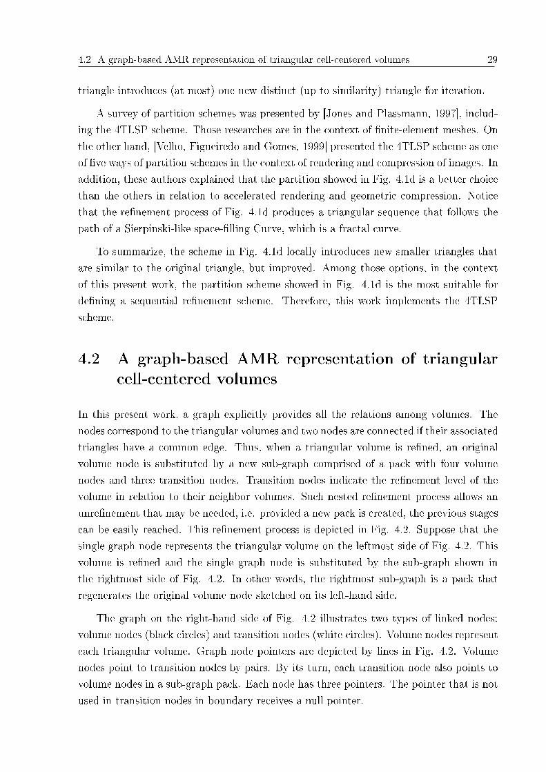
In this present work, a graph explicitly provides all the relations among volumes. Thenodes correspond to the triangular volumes and two nodes are connected if their associatedtriangles have a common edge. Thus, when a triangular volume is rened, an originalvolume node is substituted by a new sub-graph comprised of a pack with four volumenodes and three transition nodes. Transition nodes indicate the renement level of thevolume in relation to their neighbor volumes. Such nested renement process allows anunrenement that may be needed, i.e. provided a new pack is created, the previous stagescan be easily reached. This renement process is depicted in Fig. 4.2. Suppose that thesingle graph node represents the triangular volume on the leftmost side of Fig. 4.2. Thisvolume is rened and the single graph node is substituted by the sub-graph shown inthe rightmost side of Fig. 4.2. In other words, the rightmost sub-graph is a pack thatregenerates the original volume node sketched on its left-hand side.
The graph on the right-hand side of Fig. 4.2 illustrates two types of linked nodes:volume nodes (black circles) and transition nodes (white circles). Volume nodes representeach triangular volume. Graph node pointers are depicted by lines in Fig. 4.2. Volumenodes point to transition nodes by pairs. By its turn, each transition node also points tovolume nodes in a sub-graph pack. Each node has three pointers. The pointer that is notused in transition nodes in boundary receives a null pointer.
4.2 A graph-based AMR representation of triangular cell-centered volumes 30
Figure 4.2: A triangular volume rened, the single graph node that represented the orig-inal triangular volume and on the mostright side a sub-graph created after a renementof the triangular volume, respectively. The opposite is performed in the unrenementprocess.
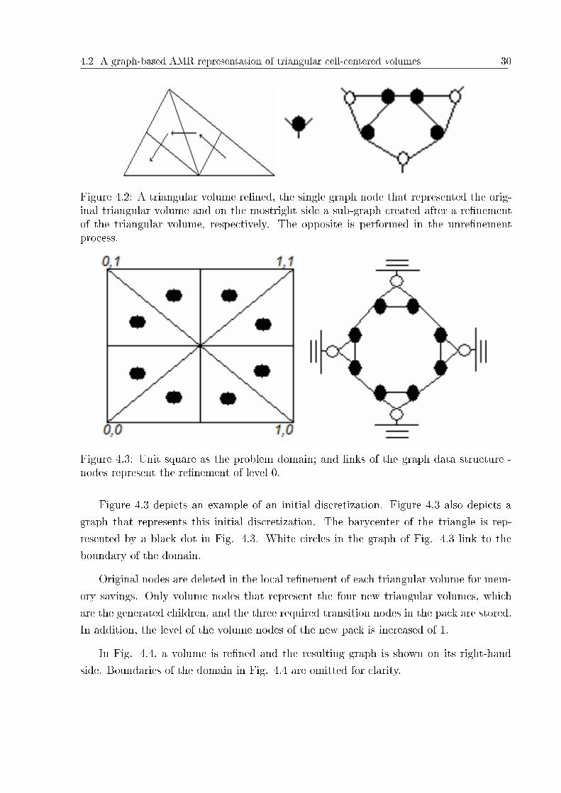
Figure 4.3: Unit square as the problem domain; and links of the graph data structure -nodes represent the renement of level 0.
Figure 4.3 depicts an example of an initial discretization. Figure 4.3 also depicts agraph that represents this initial discretization. The barycenter of the triangle is rep-resented by a black dot in Fig. 4.3. White circles in the graph of Fig. 4.3 link to theboundary of the domain.
Original nodes are deleted in the local renement of each triangular volume for mem-ory savings. Only volume nodes that represent the four new triangular volumes, whichare the generated children, and the three required transition nodes in the pack are stored.In addition, the level of the volume nodes of the new pack is increased of 1.
In Fig. 4.4, a volume is rened and the resulting graph is shown on its right-handside. Boundaries of the domain in Fig. 4.4 are omitted for clarity.

4.3 Graph simplication for volumes of the same level 31
Figure 4.4: Renement example with triangular volumes; and graph with transition andvolume nodes that forms the scheme of this triangular volume renement, respectively.
Figure 4.5: Renement of another volume depicted in Fig. 4.4, its graph representation,and graph simplication, respectively.
4.3 Graph simplication for volumes of the same level
Figure 4.5 illustrates another renement of the discretized domain of Fig. 4.4, its graphrepresentation, and the simplication of the graph, respectively. More precisely, since vol-umes have the same renement level, namely, their vertices are coincident; the mostrighthand-side graph of Fig. 4.5 illustrates its simplication.
4.4 Generalization of the renement scheme
During time evolution, the mesh is rened and a linear system must be solved each timestep. As long as the dierence in scale of ux between two neighbor volumes is large, onecould choose to rene the volume in more than four new volumes. Table I describes theoptions.

4.4 Generalization of the renement scheme 32
Table I: Number of transition and mesh nodes in a pack.n L Transition nodes Volume nodes1 +1 3 42 +2 9 163 +3 21 644 +4 45 2565 +5 93 1024. . . . . . . . . . . .
n +n 3 ·n−1∑i=0
2i 4n
In Table I, column n means in how much levels (L) the pack is rened. For example,the experimental tests presented in this work shown=1. The last line of Table I generalizesthe proposal. Namely, one can choose n (n|n ∈ N∗) in order to rene a volume in 4n
volumes in the new pack. Hence, the pack will have3 ·n−1∑i=0
2i new transition nodes, wherethe sum until n − 1 is because the levels are nested. Moreover, the sum of 2i is becauseeach edge is bisected and one transition node links two volumes. In addition, the sum ismultiplied by three due to the number of edges of (the original volume: level 0) a triangle.There will be
3 · 2n−1 transition nodes in level +n,3 · 2n−2 transition nodes in level +(n-1),
. . .
3 · 20 transition nodes in level +1.
Figure 4.6 shows an example with n=2. Hence, there are sixteen (42) volumes inthe new pack, sixteen volume nodes and nine (3 · (1 + 2)) transition nodes in the newsub-graph, being three (3 · 20) transition nodes of level n+1 and six (3 · 21) transitionnodes of level n+2.
Observing the new pack in Fig. 4.6, one can notice that columns (and lines) and lineshave odd number of volumes. Clearly, the sum of the number of volumes of the columns(or the lines) results in the number of volumes of the pack. Consequently, one can write
[∀n ∈ N |n even ∧ 2n =2
n2∑
i=1
(2i− 1)] since
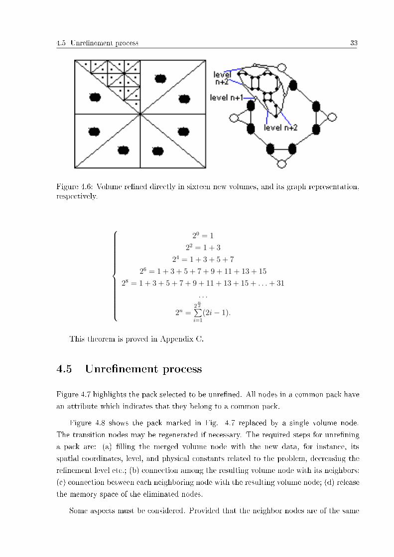
4.5 Unrenement process 33
Figure 4.6: Volume rened directly in sixteen new volumes, and its graph representation,respectively.
20 = 1
22 = 1 + 3
24 = 1 + 3 + 5 + 7
26 = 1 + 3 + 5 + 7 + 9 + 11 + 13 + 15
28 = 1 + 3 + 5 + 7 + 9 + 11 + 13 + 15 + . . . + 31
. . .
2n =2
n2∑
i=1
(2i− 1).
This theorem is proved in Appendix C.
4.5 Unrenement process
Figure 4.7 highlights the pack selected to be unrened. All nodes in a common pack havean attribute which indicates that they belong to a common pack.
Figure 4.8 shows the pack marked in Fig. 4.7 replaced by a single volume node.The transition nodes may be regenerated if necessary. The required steps for unreninga pack are: (a) lling the merged volume node with the new data, for instance, itsspatial coordinates, level, and physical constants related to the problem, decreasing therenement level etc.; (b) connection among the resulting volume node with its neighbors;(c) connection between each neighboring node with the resulting volume node; (d) releasethe memory space of the eliminated nodes.
Some aspects must be considered. Provided that the neighbor nodes are of the same
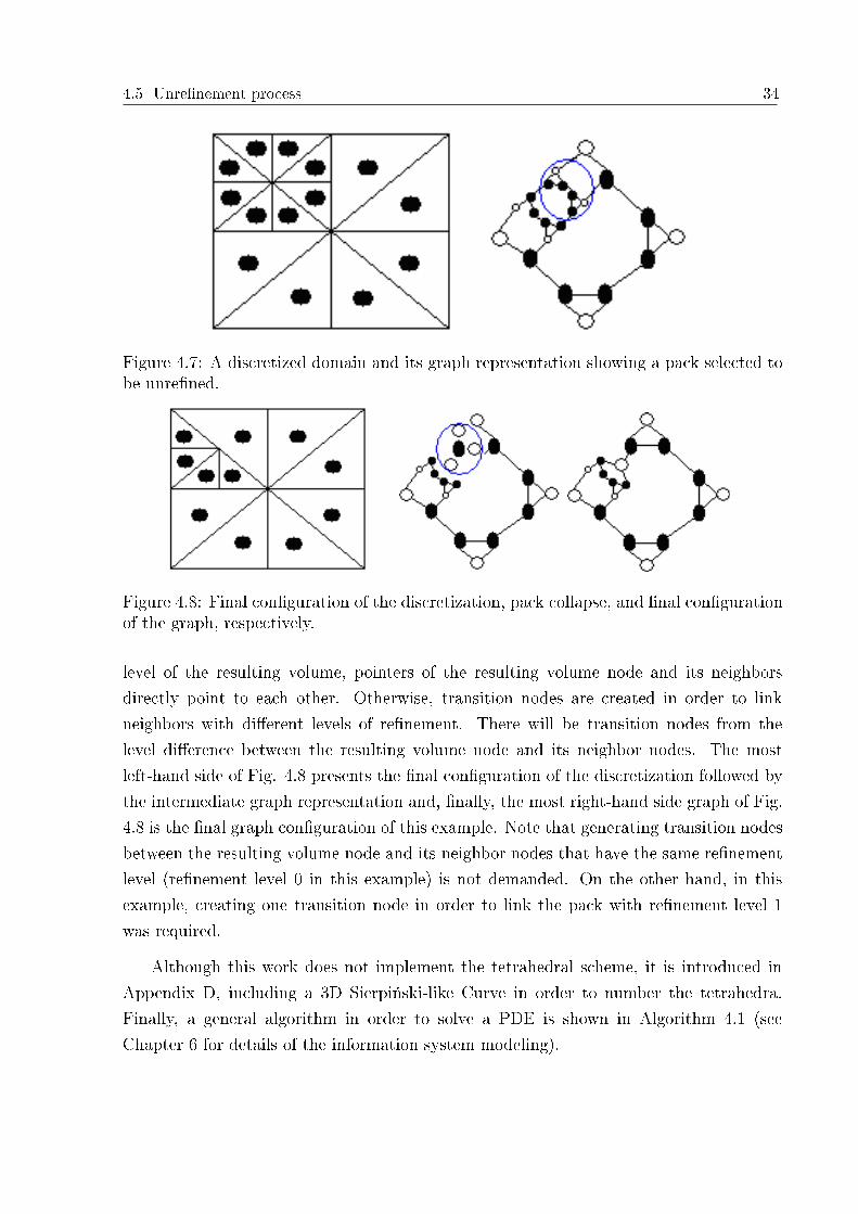
4.5 Unrenement process 34
Figure 4.7: A discretized domain and its graph representation showing a pack selected tobe unrened.
Figure 4.8: Final conguration of the discretization, pack collapse, and nal congurationof the graph, respectively.
level of the resulting volume, pointers of the resulting volume node and its neighborsdirectly point to each other. Otherwise, transition nodes are created in order to linkneighbors with dierent levels of renement. There will be transition nodes from thelevel dierence between the resulting volume node and its neighbor nodes. The mostleft-hand side of Fig. 4.8 presents the nal conguration of the discretization followed bythe intermediate graph representation and, nally, the most right-hand side graph of Fig.4.8 is the nal graph conguration of this example. Note that generating transition nodesbetween the resulting volume node and its neighbor nodes that have the same renementlevel (renement level 0 in this example) is not demanded. On the other hand, in thisexample, creating one transition node in order to link the pack with renement level 1was required.
Although this work does not implement the tetrahedral scheme, it is introduced inAppendix D, including a 3D Sierpi«ski-like Curve in order to number the tetrahedra.Finally, a general algorithm in order to solve a PDE is shown in Algorithm 4.1 (seeChapter 6 for details of the information system modeling).

4.5 Unrenement process 35
Algorithm 4.1: Solving a PDE.beginboolean: continueRening← true;initialize grid;initialize φ with initial conditions;FOR t← initial step time UNTIL t < tfinal STEP ∆t
WHILE (continueRening) renement iterations initializes entries of the grid discretization matrix determines values of all entries in the matrix and the independent vector b each line of the coecient matrix is a linked list Element of the volume node bi is an attribute of the volume node set discretization matrix (t);Conjugate Gradient Method;release memories of the Element linked lists;continueRening← ReneGrid ();
end-WHILE;unrenement;
end-FOR;draw Sierpinski-like Curve;end.

Chapter 5
Mesh total ordering
Mesh volumes should have some ordering so that each volume is related to each line ofthe resulting linear system in an implicit formulation. Thus, creating a direct strip isappropriate. [Velho, Figueiredo and Gomes, 1999] described a dual graph for triangularmesh in order to build triangle strips by heuristics. Those authors considered severalissues related to paths on the dual graph of general triangular meshes.
A triangular sequence designates a sequential triangulation, as well as its generaliza-tions. A triangular sequence denes a total-order relation on the set of triangles of amesh. Dividing a triangular mesh in a collection of sub-triangulations so that each newpack is a triangular sequence is always possible [Velho, Figueiredo and Gomes, 1999].
[Velho, Figueiredo and Gomes, 1999] also explained that a generalized sequential tri-angulation, or Hamiltonian triangulation, is a triangulation in which there is an orderingT1, . . . , TN of all its triangles so that two consecutive trianglesTj and Tj+1 share an edge.A path in a graph is said to be Hamiltonian if it visits all nodes in the graph exactly once.They also claimed that each triangle in a Hamiltonian triangulation has an entry and anexit edges with respect to the Hamiltonian ordering. The knowledge of these edges com-pletely characterizes the sequence. Geometrically, a generalized triangular sequence canbe represented by drawing an oriented path on the mesh domain that visits each trianglecrossing its entry and exit edges, called a sequential path (see Fig. 4.1d). Likewise, thescheme proposed here always generates a generalized sequential triangulation.
Finite volumes of the mesh must be numbered so that the corresponding linear systemhas each row matching a specic nite volume. Thus, similarly to[Velho, Figueiredo and Gomes, 1999], this present work builds the triangle strip whilecreating a triangulation. This work proposes a dynamic Sierpi«ski-like space-lling Curvefor total ordering of a graph-based triangular mesh.

5.1 Sierpi«ski Curve 37
Figure 5.1: Generator process of the Sierpi«ski Curve through equilateral triangles dividedinto 4, 10 and 22 triangles, respectively.
Figure 5.2: Sierpi«ski Curve generation.
5.1 Sierpi«ski Curve
A curve (with endpoints) is a continuous function whose domain is the unit interval[0, 1]2. Moreover, the limit of the sequence given by curves of order1, 2, . . ., is the curvethat passes through each point in the unit square [0; 1]2, or in a closed continuous surface.Furthermore, space-lling curves are curves whose ranges contain the entire 2D unit square(or the 3D unit cube).
The Sierpi«ski Curve is a space-lling curve proposed by [Sierpi«ski, 1912] and com-plemented in [Sierpi«ski, 1916]. Moreover, Sierpi«ski Curves are a recursively denedsequence of continuous closed plane fractal curves, which in the limitn→∞ completelyll the unit square: thus, their limit curve is an example of a space-lling curve. Sierpi«skiCurves in uniform successive renement in equilateral triangles are depicted in Fig. 5.1.
Figure 5.2 depicts another example of Sierpi«ski Curve generation. As long as thedomain shape is the left-hand side triangle of Fig. 5.2, and also the triangles are uniformlyrened, the third level of renement and ordering is such as the right-hand side curve ofFig. 5.2. Figure 5.3 depicts Sierpi«ski Curve ordering scalene triangles.
Consider the 2D Laplace Equation with equal prescribed boundary condition in allsides of the unit square. Let the Dirichlet Problem given by
∇2φ = 0 in Ω, φ = f on ∂Ω, (5.1)
Figure 5.3: Sierpi«ski Curve ordering scalene triangles.

5.1 Sierpi«ski Curve 38
Figure 5.4: Sierpi«ski Curves in a unit square with23, 23, . . ., 211 volumes.
where φ is the dependent variable of the EDP, Ω is a limited domain in R2, and f is adened smooth function on boundary ∂Ω.
In 1902, Jacques Salomon Hadamard (1865-1963) claimed that, for a mathematicalproblem correspond to reality, the following basic conditions should be satised: thesolution must exist (existence); the solution must be determined by data of a unique form(unicity); and the solution must depend on data of continual form (stability). Problem5.1 is well-posed in the sense of Hadamard according to [Zachmanoglou and Thoe, 1986].
Consider now the approximation of 5.1 in a unit square. Following the Finite VolumeMethod basic formulation for irregular meshes gives
∮∇φ · ~nd(∂vi) = 0, (5.2)
where ~n is the normal outward vector of control volumevi and ∂vi represents the boundaryof the control volume vi. After numerical integration, the numerical solution of equation5.2 is illustrated in Fig. 5.4 with constant boundary conditions. Moreover, through settingf as a constant function, Fig. 5.4 illustrates nine levels of the Sierpi«ski Curve.

5.2 Sierpi«ski-like Curve for the total-order relation on the triangular volumes of the mesh 39
Figure 5.5: Successive adaptive renements with volumes ordered by a Sierpi«ski-likeCurve on the right-hand side of each discretization.
5.2 Sierpi«ski-like Curve for the total-order relation onthe triangular volumes of the mesh
In [Gonzaga and Kischinhevsky, 2008], a non-regular Sierpi«ski Curve for total orderingof volumes of a discretized mesh was introduced. It is generated by a double-linked list.Exemplifying, Fig. 5.5 sketches successive adaptive renements by volume bisection in aquadrangular domain with triangular volumes ordered by a Sierpi«ski-like Curve. Thisscheme allows straightforward update of the linked list for mesh node ordering. Thismeans that, in the sense of data structures, this adaptive renement scheme of triangularvolumes enables straightforward update of the linked list in the modication of volumenodes in the adaptive renement process during the evolution of the partial dierentialequation.
In summary, since triangular volumes are adaptively rened, this work uses a Sierpi«ski-like Curve. The modication is that volumes are adaptively rened by sucessive bisections.
Chapter 6
Experimental tests
Tests show numerical results in the Laplace (elliptic problem), Heat Conduction (parabolicproblem), Wave (hyperbolic problem) Equations and at-plate Boundary Layer Problemperformed in an Intelr CeleronTM 2.6GHz (approximated) processor with 256MB DDRSDRAM (plus 360MB virtual memory) and XGA display integrated with 32MB VRAMvideo memory.
In all tests accomplished, the linear systems presented sparse, symmetric and positive-denite coecient matrices. It is very likely that this scheme always produces matriceswith those properties.
Linear-system solvers based on the minimization of functionals were easily employedin this work. Specically, the Conjugate Gradient Method [Hestenes and Stiefel, 1952]was employed. This method is one of the most proeminent iterative methods for solvingsparse systems of linear equations. Notice that a pre-conditioner was not used.
Before showing the experimental tests, the modeling information is briey presentedas well as the renement criteria adopted.
6.1 Information system modeling using UML
These object-oriented projects were coded in C++ language using OpenGL [OpenGL, 1993].The main classes of the modeling are described in Fig. 6.1. The Grid object is composedby at least eight Volume objects. The Volume objects are strongly related to the Gridone. Namely, if the Grid object is deleted, so are all the Volume instances. Afterwards, aVolume instance has a constant number of Side objects. In the codes of this work, eachVolume instance has three Side objects. Moreover, although the Side was implemented asa class, the objects are parts of the Volume object. Namely, the Side objects are allocatedwhen the Volume objects are allocated. However, the code is prepared to be implemented

6.2 Renement criteria 41
Figure 6.1: Simplied diagram class of this work.
with general polygonal volumes. Furthermore, if one codes volumes withn edges, thevolume will have n Side objects.
A Volume class is also composed by one Element class. Moreover, an Element classis strongly related to the volume it belongs to: if the Volume object is deleted, so is theassociated Element object.
The Grid class is the main one of the implementation. In this class, the data struc-tures, the mesh node numbering, the adaptive mesh renement (AMR) algorithm and theConjugate Gradient Method calling are programmed. Next, the Volume class is responsi-ble for implementing the volume nodes. It stores the connectivity information of the meshnodes, and in its objects the Sierpinski-like Curve is implemented, among other functions.Subsequently, a Side object stores geometrical information about the edge (that it repre-sents) of the volume which it belongs to. Finally, in the Element class, a simple linkedlist is implemented. In this linked list, the non-null coecients of a line (related to thespecic volume) of the resulting linear system are stored.
6.2 Renement criteria
The renement criteria is based on the gradient of the edge between two neighbor volumes.Namely, provided that the gradient of the ux in an edge is greater than a renementquota established by the user, both volumes are rened. The choice of the user is basedon the requirements of a larger or smaller renement in certain regions of the domainwhere there is larger or smaller variation in the solution behavior. Since a large varia-tion in certain regions may occur in the analytical solution, a large dierence of uxesamong neighboring volumes does not necessarily mean that there is a large variation inthe dierence between the approximation and the analytical solution. Therefore, thosecriteria chosen by the user overestimate the number of renements needed. Similarlyto [Burgarelli, Kischinhevsky and Biezuner, 2006], an error estimator, tailored to specicapplications, can be used in order to improve the performance of the algorithm.
Since this present approach tailors the work proposed in [Schneider and Maliska, 2002],

6.3 Laplace Equation (elliptic problem) 42
Figure 6.2: Sierpinski-like Curve of the AMR scheme applied to the Laplace Equation.
this choice could present a less homogeneous distribution of the edge sizes and the sizesof the proper control volumes. For this reason, seeking a smooth (or graded) transitionamong neighbor volumes in the experimental tests, a limit of the dierence of renementlevels between neighbor volumes was implemented. That was performed in order to avoidnumerical oscillations, though the scheme and the graph data structure allow any dier-ence in the level of renements between neighbor volumes. In other words, the areas ofneighboring triangles do not dier dramatically.
6.3 Laplace Equation (elliptic problem)
[Gonzaga et al., 2008] approximated the problem given in 5.1, where on top, bottom,and left sides of the unit square present prescribed boundary condition with a uniqueconstant f . On the other hand, right side of the unit square presents a dierent valuefor f . Moreover, Fig. 6.2 illustrates the Sierpinski-like Curve of this AMR scheme.Furthermore, Fig. 6.2 shows the nal mesh conguration after eight time steps using1.5 in the renement criteria. The mesh is comprised of 4421 volumes, whose ConjugateGradient Method converges after 729 iterations.

6.4 Heat Conduction Equation (parabolic problem) 43
6.4 Heat Conduction Equation (parabolic problem)
Consider the 2D Heat Conduction Equation with continuous initial and boundary data
φt = ∇2φ
φ(u, 0) = f(u), u ∈ Ω, f(u) ≡ 0,
φ(u, t) = g(u), u(u) ∈ Ω, t ≥ 0, (6.1)
where the bounded Ω ⊂ R2, thus, u = (x, y), and f is a smooth function limited in Ω.Problem 6.1 is well-dened in the sense of Hadamard [Zachmanoglou and Thoe, 1986].Therefore, consider the approximation of 6.1 in a unit square. Consider now the FiniteVolume Method (FVM) basic implicit formulation for irregular meshes
Mk+1P φk+1
P −∆t
∮
∂Ω
∇φk+1 · ~nd(∂Ω) = MkP φk
P , (6.2)
where M represents the area of4P and ∆t = 0.1.
Boundary conditions on top, bottom and left sides of the unit square have a uniqueprescribed boundary value f and right side has a dierent value. Figure 6.3 illustratesthe nal mesh conguration after ten time steps (∆t = 0.1) using 1.0 in the renementcriteria and seven maximum renement levels for each volume. The mesh is comprised of5285 volumes, whose Conjugate Gradient Method converges in 578 iterations.
Figure 6.4 illustrates a test with boundary conditionx−y and the renement criteriais 0.05. Moreover, Fig. 6.4 shows the nal discretizations after ten time steps (∆t = 0.1)with six maximum levels of renement for each volume making up 6110 volumes whoseConjugate Gradient Method converges in 10 rounds comprising from 520 to 181 iterations.
Figure 6.5 illustrates a test with boundary conditionx2 − y2, 0.07 as the renementcriteria and ten time steps where∆t = 0.1. Moreover, Fig. 6.5 shows the nal discretiza-tions with seven maximum levels of renement for each volume making up 4472 volumeswhose Conjugate Gradient Method converges in 10 rounds comprising from 640 to 278iterations.
6.4.1 Performance of the renement process
[Burgarelli, Kischinhevsky and Biezuner, 2006] showed those boundary conditions of theapproximation to the Heat Conduction Equation in order to demonstrate the performance

6.4 Heat Conduction Equation (parabolic problem) 44
Figure 6.3: Final mesh conguration of an AMR approximation to the Heat ConductionEquation.
Figure 6.4: Final time step of an AMR approximation to the Heat Conduction Equationwith boundary condition: x− y.
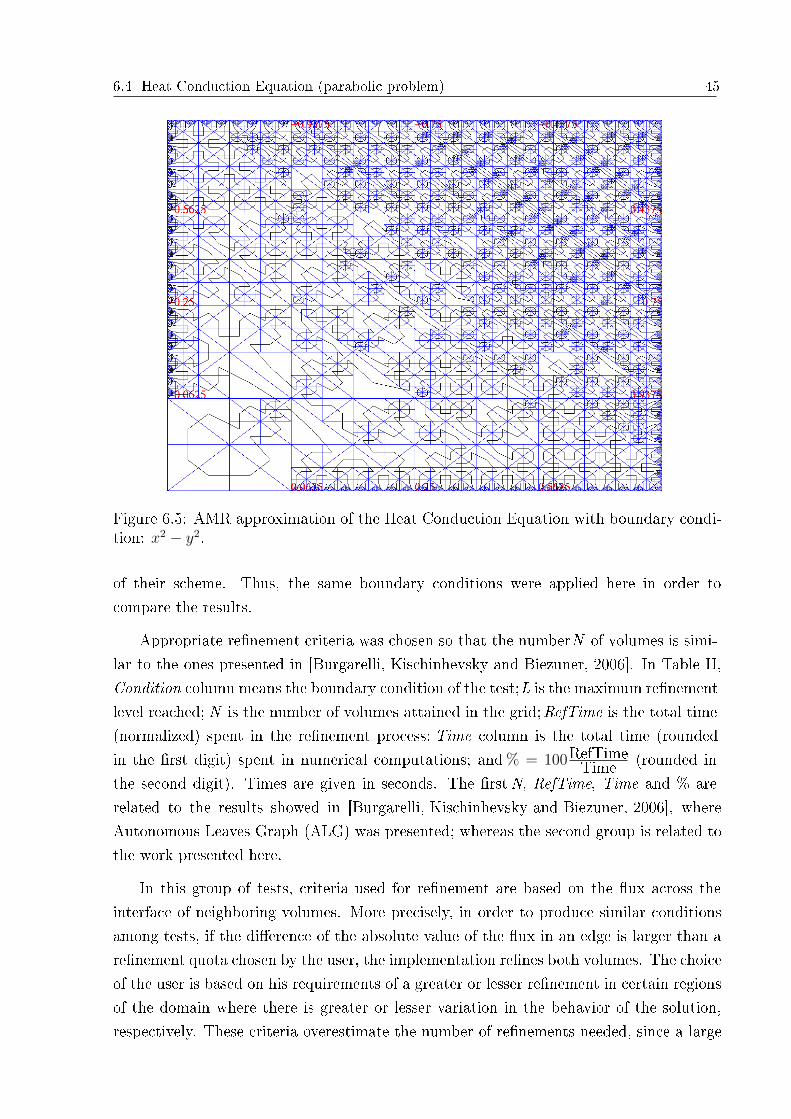
6.4 Heat Conduction Equation (parabolic problem) 45
Figure 6.5: AMR approximation of the Heat Conduction Equation with boundary condi-tion: x2 − y2.
of their scheme. Thus, the same boundary conditions were applied here in order tocompare the results.
Appropriate renement criteria was chosen so that the numberN of volumes is simi-lar to the ones presented in [Burgarelli, Kischinhevsky and Biezuner, 2006]. In Table II,Condition column means the boundary condition of the test;L is the maximum renementlevel reached; N is the number of volumes attained in the grid;RefTime is the total time(normalized) spent in the renement process; Time column is the total time (roundedin the rst digit) spent in numerical computations; and% = 100RefTime
Time (rounded inthe second digit). Times are given in seconds. The rstN, RefTime, Time and % arerelated to the results showed in [Burgarelli, Kischinhevsky and Biezuner, 2006], whereAutonomous Leaves Graph (ALG) was presented; whereas the second group is related tothe work presented here.
In this group of tests, criteria used for renement are based on the ux across theinterface of neighboring volumes. More precisely, in order to produce similar conditionsamong tests, if the dierence of the absolute value of the ux in an edge is larger than arenement quota chosen by the user, the implementation renes both volumes. The choiceof the user is based on his requirements of a greater or lesser renement in certain regionsof the domain where there is greater or lesser variation in the behavior of the solution,respectively. These criteria overestimate the number of renements needed, since a large

6.4 Heat Conduction Equation (parabolic problem) 46
dierence of uxes does not necessarily mean that there is a large variation in the dierencebetween the approximate and exact solutions, for this variation can already occur in theexact solution. The tests were performed choosing∆t = 0.1 with the program runninguntil t = 10∆t. The initial conditions were set asf(x, 0) = 0. In the level L, the minimumvolume size attained is 2−L.
Results are summarized in Table II where comparisons between the results from[Burgarelli, Kischinhevsky and Biezuner, 2006] and this present work can be carried outsince the number of volumes is similar in the simulations. Moreover, Table II shows thatmost of the computing time is spent in the core of the computation, leaving very lowprocessing time to renement stages. Furthermore, the higher resolution of results is re-quired, the more the computational cost in renement stages decreases. Notice that sincethe hardware that [Burgarelli, Kischinhevsky and Biezuner, 2006] obtained their resultsis not known, the comparison is performed in percentual as described.
Table II: Numerical results for the Heat Conduction Equation.Tests Quadrangular ALG Triangular AMR scheme
Condition L N RefTime Time % N RefTime Time %5 856 6.8 · 10−3 5.6 · 10−2 12.1 845 1.3 · 10−2 1.5 0.89
g(x, y) = 10 6 3016 1.9 · 10−2 0.8 2.4 2906 4.1 · 10−2 13.1 0.327 3580 3.5 · 10−2 2.5 1.4 3755 8.6 · 10−2 29.6 0.295 934 7.5 · 10−3 0.2 3.8 956 8.1 · 10−3 1.5 0.53
g(x, y) = x− y 6 4090 5.0 · 10−2 3.2 1.6 4028 4.5 · 10−2 21.8 0.237 15682 1.2 · 10−1 21.6 0.6 15734 2.1 · 10−1 285.5 0.07
g(x, y) = x2 − y2 6 3529 3.4 · 10−2 4.7 0.7 3431 7.7 · 10−3 37.5 0.027 12442 1.2 · 10−1 28.6 0.4 12479 2.9 · 10−2 282.9 0.01
According to Table II, the computing time spent in the renement stage of this presentwork is smaller than ALG. This is mainly because these points:
i) Dierence in the complexity of the algorithms that implement the space-llingcurves in both approaches. In the original quadrangular ALG,[Burgarelli, Kischinhevsky and Biezuner, 2006] tailored the Hilbert Curve for this issue.Moreover, the authors proposed a Modied Hilbert Curve (MHC) in order to number thevolumes. In this present work, a Sierpi«ski-like Curve is employed;
ii) Searching connectivity information in order to adjust the pointers of the graphnodes. The original quadrangular ALG scans each graph node from (a set of) four pointerswhereas this present approach scans each graph node from (a set of) three pointers.

6.4 Heat Conduction Equation (parabolic problem) 47
6.4.1.1 Complexity analysis of the space-lling curves: MHC and Sierpi«ski-like Curve
i) Complexity analysis of the MHC
The MHC algorithm requires to nd the local shape of the Hilbert Curve for each localrenement. Namely, the local curve can have four shapes: @, A, u and t. Algorithm 6.1evaluates which local shape the new pack is.
Algorithm 6.1: Evaluate the Hilbert Shape.HilbertShape (integer: volHilbertCoordinate, integer: volRenementLevel): integerbegininteger: i← 0, j, k;matrix hilbertTable[4:4]: integer;hilbertTable[0][0]← 1; hilbertTable[0][1]← 0;hilbertTable[0][2]← 0; hilbertTable[0][3]← 3;hilbertTable[1][0]← 0; hilbertTable[1][1]← 1;hilbertTable[1][2]← 1; hilbertTable[1][3]← 2;hilbertTable[2][0]← 3; hilbertTable[2][1]← 2;hilbertTable[2][2]← 2; hilbertTable[2][3]← 1;hilbertTable[3][0]← 2; hilbertTable[3][1]← 3;hilbertTable[3][2]← 3; hilbertTable[3][3]← 0;FOR k ← 1 UNTIL volRenementLevel STEP 1 DO
In computing, the modulo operation nds theremainder of division of one number by another.
j ← volHilbertCoordinate modulo 4;i ← hilbertTable[i][j];volHilbertCoordinate← vollHilbertCoordinate / 4;
end-FOR;RETURN i;end-HilbertShapeNumber.
· · ·integer: numberOfHilbertShape;

6.4 Heat Conduction Equation (parabolic problem) 48
Figure 6.6: Volume ordering in a local triangular renement.
numberOfHilbertShape← HilbertShape (volHilbertCoordinate, volRenementLevel+1);IF (numberOfHilbertShape = 0) Shape: @
11 changes + 1 condition ELSE IF (numberOfHilbertShape = 1) Shape: t
11 changes + 1 condition ELSE IF (numberOfHilbertShape = 2) Shape: A
11 changes + 1 condition ELSE IF (numberOfHilbertShape = 3) Shape: u
11 changes + 1 condition · · ·
Analysing Algorithm 6.1, the core of the computation is the instruction FOR. Theloop in the instruction FOR performs volRenementLevel times and it denes the orderof growth of the running time of the algorithm. Therefore, MHC ∈ O(L), where Lis the level of renements of the rened pack. Moreover, since the instruction FORruns volRenementLevel times, it denes the order of growth of the running time of thealgorithm. CHM could store in each node the volRenementLevel already evaluated inorder to improve its eciency.
ii) Complexity analysis of the Sierpi«ski-like_Curve
Figure 6.6 shows a local renement of a triangle. Since the local Sierpi«ski-like Curveorders the new pack starting (or nishing in) from volume d1 and nishing (or startingfrom) in volume d2, the curve can link: A→ d1 → · · · d2 → B; A → d1 → · · · d2 →C; or B → d2 → · · · d1 → C; and the path from B/C to A/B, respectively, since it isimplemented by a double-linked list.
Algorithm 6.2 presents a solution of the local Sierpi«ski-like Curve.
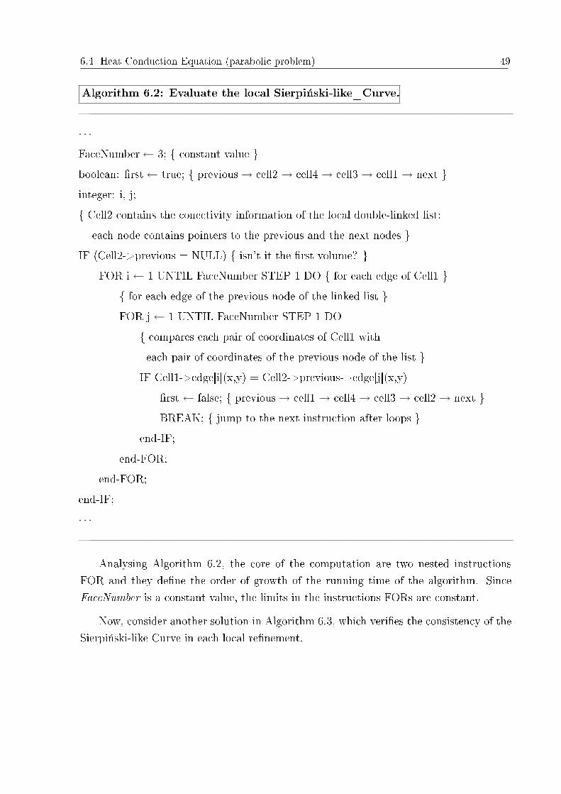
6.4 Heat Conduction Equation (parabolic problem) 49
Algorithm 6.2: Evaluate the local Sierpi«ski-like_Curve.· · ·FaceNumber← 3; constant value boolean: rst← true; previous→ cell2 → cell4 → cell3 → cell1 → next integer: i, j; Cell2 contains the conectivity information of the local double-linked list:
each node contains pointers to the previous and the next nodes IF (Cell2->previous = NULL) isn't it the rst volume?
FOR i ← 1 UNTIL FaceNumber STEP 1 DO for each edge of Cell1 for each edge of the previous node of the linked list FOR j ← 1 UNTIL FaceNumber STEP 1 DO
compares each pair of coordinates of Cell1 witheach pair of coordinates of the previous node of the list
IF Cell1->edge[i](x,y) = Cell2->previous->edge[j](x,y)rst ← false; previous→ cell1 → cell4 → cell3 → cell2 → next BREAK; jump to the next instruction after loops
end-IF;end-FOR;
end-FOR;end-IF;· · ·
Analysing Algorithm 6.2, the core of the computation are two nested instructionsFOR and they dene the order of growth of the running time of the algorithm. SinceFaceNumber is a constant value, the limits in the instructions FORs are constant.
Now, consider another solution in Algorithm 6.3, which veries the consistency of theSierpi«ski-like Curve in each local renement.
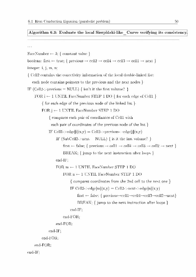
6.4 Heat Conduction Equation (parabolic problem) 50
Algorithm 6.3: Evaluate the local Sierpi«ski-like_Curve verifying its consistency.· · ·FaceNumber← 3; constant value boolean: rst← true; previous→ cell2 → cell4 → cell3 → cell1 → next integer: i, j, m, n; Cell2 contains the conectivity information of the local double-linked list:
each node contains pointers to the previous and the next nodes IF (Cell2->previous = NULL) isn't it the rst volume?
FOR i ← 1 UNTIL FaceNumber STEP 1 DO for each edge of Cell1 for each edge of the previous node of the linked list FOR j ← 1 UNTIL FaceNumber STEP 1 DO
compares each pair of coordinates of Cell1 witheach pair of coordinates of the previous node of the list
IF Cell1->edge[i](x,y) = Cell2->previous->edge[j](x,y)IF (SubCell2->next = NULL) is it the last volume?
rst ← false; previous→ cell1 → cell4 → cell3 → cell2 → next BREAK; jump to the next instruction after loops
end-IF;FOR m← 1 UNTIL FaceNumber STEP 1 DO
FOR n ← 1 UNTIL FaceNumber STEP 1 DO compares coordinates from the 2nd cell to the next one IF Cell2->edge[m](x,y) = Cell2->next->edge[n](x,y)
rst ← false; previous→cell1→cell4→cell3→cell2→nextBREAK; jump to the next instruction after loops
end-IF;end-FOR;
end-FOR;end-IF;
end-FOR;end-FOR;
end-IF;

6.4 Heat Conduction Equation (parabolic problem) 51
· · ·
Algorithm 6.2 or 6.3 is followed by Algorithm 6.4.
Algorithm 6.4: Sierpi«ki-like_Curve links the nodes of the new pack.· · ·IF (rst = true) update the double-linked list
IF (Cell2->next = true) Cell2->next->previous← Cell1;Cell1->next← Cell2->next;Cell3->next← Cell1;Cell4->next← Cell3;Cell2->next← Cell4;Cell1->previous← Cell3;Cell3->previous← Cell4;Cell4->previous← Cell2;
ELSECell2->previous->next← Cell1;Cell1->next← Cell3;Cell3->next← Cell4;Cell4->next← Cell2;Cell1->previous← Cell2->previous;Cell3->previous← Cell1;Cell4->previous← Cell3;Cell2->previous← Cell4;
end-IF.· · ·
Since the implementation was coded in order to use volumes withn edges, FaceNumberdenotes the number of edges of the volume. Even employing the Algorithm 6.3 in whichthere are four nested intructions FOR, in a superior quota, there are34 conditions, i.e. thelimits of the loops are constant values that do not depend on any input of the algorithm(or the level of the renement). Therefore, Sierpi«ski-like_Curve∈ O(1).

6.5 Wave Equation (hyperbolic problem) 52
Emphasizing, Ω denes an inferior quota for the growth of the procedure. Necessarily,CHM performs the main loopvolRenementLevel times. Therefore, CHM∈ Ω(L). On theother hand, Sierpi«ski-like_Curve may nd the node in one round even in the Algorithm6.3. Thus, Algorithm 6.2 or 6.3 may break a loop if it nds the node being searched.Therefore, Sierpi«ski-like_Curve∈ Ω(1).
Corollary. CHM ∈ Θ(L) ∧ Sierpi«ski-like_Curve ∈ Θ(1). (6.3)
Proof. Straightforwardly, using [Cormen et al., 2001]
Theorem. ((∀f(n), g(n))(f(n) ∈ Θ(g(n))⇔ f(n) ∈ O(g(n)) ∧ f(n) ∈ Ω(g(n)))).¤ (6.4)
6.4.1.2 Quadrangular volumes × Triangular volumes
In the local renement, each volume node is scanned in order to adjust the pointers of thenew pack in relation to the original node. Each volume node is scanned from (a set of)four pointers in the quadrangular original ALG. On the other hand, each volume node isscanned from (a set of) three pointers in this present work. At a rst sight, this could notcontribute signicantly; however, with a large number of volumes (nodes) rened afterseveral time steps, this may contribute to the dierence of performance presented in TableII.
In summary, there are two main dierences: i) complexity of the space-lling curvealgorithms; and ii) number of pointers when searching conectivity information for adjust-ing the pointers of the graph nodes. Those dierences in the approaches may be relevantif applied to several of nodes after n time steps.
6.5 Wave Equation (hyperbolic problem)
The 2D rst-order Wave Equation is
∂φ
∂t+ c1
∂φ
∂x+ c2
∂φ
∂y= 0. (6.5)
Consider two waves moving along opposite directions with the coordinated axes.Namely, one wave moves diagonally from (0,0) to (1,1) and the other moves from (1,1) to(0,0). In particular, let c1 = c2 =
√2
2and φ = φ1(x, y, t) + φ2(x, y, t), where φ1 satises
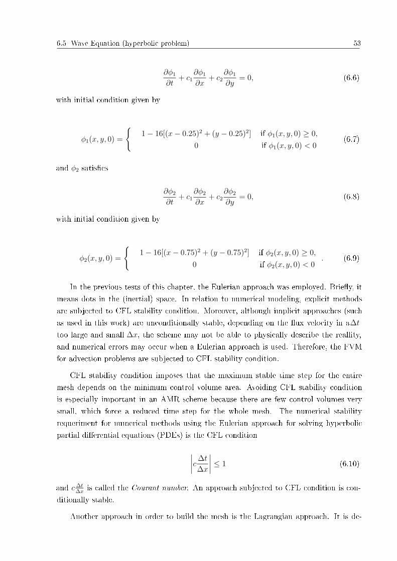
6.5 Wave Equation (hyperbolic problem) 53
∂φ1
∂t+ c1
∂φ1
∂x+ c2
∂φ1
∂y= 0, (6.6)
with initial condition given by
φ1(x, y, 0) =
1− 16[(x− 0.25)2 + (y − 0.25)2] if φ1(x, y, 0) ≥ 0,
0 if φ1(x, y, 0) < 0(6.7)
and φ2 satises
∂φ2
∂t+ c1
∂φ2
∂x+ c2
∂φ2
∂y= 0, (6.8)
with initial condition given by
φ2(x, y, 0) =
1− 16[(x− 0.75)2 + (y − 0.75)2] if φ2(x, y, 0) ≥ 0,
0 if φ2(x, y, 0) < 0. (6.9)
In the previous tests of this chapter, the Eulerian approach was employed. Briey, itmeans dots in the (inertial) space. In relation to numerical modeling, explicit methodsare subjected to CFL stability condition. Moreover, although implicit approaches (suchas used in this work) are unconditionally stable, depending on the ux velocity in a∆t
too large and small ∆x, the scheme may not be able to physically describe the reallity,and numerical errors may occur when a Eulerian approach is used. Therefore, the FVMfor advection problems are subjected to CFL stability condition.
CFL stability condition imposes that the maximum stable time step for the entiremesh depends on the minimum control volume area. Avoiding CFL stability conditionis especially important in an AMR scheme because there are few control volumes verysmall, which force a reduced time step for the whole mesh. The numerical stabilityrequeriment for numerical methods using the Eulerian approach for solving hyperbolicpartial dierential equations (PDEs) is the CFL condition
∣∣∣∣c∆t
∆x
∣∣∣∣ ≤ 1 (6.10)
and c ∆t∆x
is called the Courant number. An approach subjected to CFL condition is con-ditionally stable.
Another approach in order to build the mesh is the Lagrangian approach. It is de-

6.5 Wave Equation (hyperbolic problem) 54
ned as forming a mesh scheme that in each time step the moviment of the parcels of the(non-inertial) uid is accompanied. Moreover, in such mesh scheme, a certain magnitudeof ux is in function of time and the element of the uid. Afterwards, the main ideaof the Eulerian-Lagrangian approach is to reconcile the advantages of both approaches,i.e. the regular distribution of the particles in time step t + ∆t is maintained, compu-tation is facilitated and it enables larger time steps than the other approaches since theEulerian-Lagrangian approach is unconditionally stable because the domain of the de-pendency of the numerical solution always include the dependency of the exact solution[Fonseca, 2005].
Thus, a Eulerian-Lagrangian approach is employed in this test. The applied procedureto nd the value in the volume that contains the coordinates of the foot of a characteristicline, i.e. the intersection point of a characteristic line with the computational domain, inthe previous instant is the Modied Method of Characteristics [Douglas and Russel, 1982].In the linear approach, if (xP , yP ) denote the coordinates of the current volume, thecoordinates (xC , yC) of the foot of the characteristic line that intersects this volume areobtained by xC = xP − c1∆t and yC = yP − c2∆t.
After calculating the coordinates of the foot of a characteristic line, one needs to ndthe volume that corresponds to these coordinates. The starting point is the volume, whichin the previous time step meets the characteristic line. The neighbors are scanned andthe walking direction is chosen through comparing the horizontal and vertical distancesbetween the barycenter of the current volume and the foot of the characteristic line. Thedirection of the largest distance is taken as the walking direction, moving thus to thecontiguous volume, which then becomes the current volume for walking, and the processcontinues until the volume that contains the foot of the characteristic line is reached.Algorithm 6.5 presents the basic algorithm for solving this problem through dynamicrenements and unrenements.
Algorithm 6.5: A Wave Equation solution.begininitialize φ with initial conditions;initial renement;store φold;WHILE (t < tfinal)
Modied Method of Characteristics;store uold;rene/unrene;

6.6 Flat-plate Boundary Layer Problem 55
Figure 6.7: AMR approximation of the Wave Equation through the Modied Method ofCharacteristics.
t = t + ∆t;end-WHILE;end.
The rst discretized domain in Fig. 6.7 shows the mesh rened for this problem atthe instant t = 0 with 272 volumes. The second discretized domain in Fig. 6.7 illustratesthe same pattern with more renements comprising of 800 volumes. Afterwards, theprogram scans the entire mesh trying detecting if there is some unrenement that fulllsthe required tolerance for the problem. Some regions are then unrened, e.g. where thesolution pack has zero value. The third discretized domain in Fig. 6.7 displays a posteriorstage of this adaptive renement and unrenement for a certain instant of time when thetwo waves overlap.
6.6 Flat-plate Boundary Layer Problem
In Physics and Fluid Mechanics, the boundary layer is the uid layer in the immediatevicinity of a bounding surface. It is important in many aerodynamic problems. Thissection presents a numerical simulation of the 2D laminar Boundary Layer Problem con-sidering a steady incompressible ow with no-slip condition on the surface. The numericalsolution for the at-plate Boundary Layer Problem is compared to its analytical solution,namely Blasius Solution. Figure 6.8, tailored from [Anderson, Tannehill and Pletcher, 1984],sketches the at-plate boundary-layer process.
Let ε = 4R, where 4 is the velocity boundary-layer thickness andR is the reference
length used in the Reynolds number [Anderson, Tannehill and Pletcher, 1984]. Using amagnitude analysis order, no term in they-momentum equation is larger than ε in the es-timated magnitude and the well-known governing Navier-Stokes Equations of viscous uidow can be greatly simplied within the boundary layer. Notably, the PDE characteristic

6.6 Flat-plate Boundary Layer Problem 56
Figure 6.8: Flat-plate boundary-layer process.
becomes parabolic, rather than the elliptical form of the full Navier-Stokes Equations.This greatly simplies the solution of the equations. Thus, the Navier-Stokes Equationsfor a 2D steady incompressible ow in Cartesian coordinates are given by the momentumand the continuity equations, i.e. the nonlinear governing PDEs in terms of dimensionalvariables are given by [Anderson, Tannehill and Pletcher, 1984]
Continuity : ∇ · φ = 0, (6.11)
Momentum : ~u∇ · φ = −1
ρ
dp
dx+ ν
∂2φ
∂y2, (6.12)
where p is pressure, ~u is the vector eld, φ(u, v) is the PDE dependent variable, ρ is theuid density and ν is the kinematic viscosity.
6.6.1 A nite volume discretization of the Boundary Layer Prob-lem
[Gonzaga, Guedes and Kischinhevsky, 2007] presented details of a quadrangular nite vol-ume discretization of the at-plate Boundary Layer Problem. In addition,[Gonzaga and Kischinhevsky, 2009] presented more details of the quadrangular nite vol-ume discretization of the Boundary Layer Problem also simulating a NACA0012 airfoil inthe domain. Tailoring their approach, the triangular nite volume discretization of Eq.(6.11) is
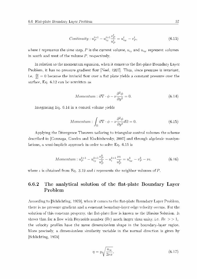
6.6 Flat-plate Boundary Layer Problem 57
Continuity : ut+1P − ut+1
iS
vtP
utP
= utiW− vt
P , (6.13)
where t represents the time step, P is the current volume, uiS and uiW represent volumesin south and west of the volume P , respectively.
In relation to the momentum equation, when it comes to the at-plate Boundary LayerProblem, it has no pressure gradient ow [Neel, 1997]. Thus, since pressure is invariant,i.e. dp
dx= 0 because the inviscid ow over a at plate yields a constant pressure over the
surface, Eq. 6.12 can be rewritten as
Momentum : ~u∇ · φ− ν∂2φ
∂y2= 0. (6.14)
Integrating Eq. 6.14 in a control volume yields
Momentum :
∫
Ω
~u∇ · φ− ν∂2φ
∂y2dΩ = 0. (6.15)
Applying the Divergence Theorem tailoring to triangular control volumes the schemedescribed in [Gonzaga, Guedes and Kischinhevsky, 2007] and through algebraic manipu-lations, a semi-implicit approach in order to solve Eq. 6.15 is
Momentum : uk+1P − uk+1
iS
vkP
ukP
− uk+1i
νι
ukP
= ukiW− vk
P − νι. (6.16)
where ι is obtained from Eq. 3.19 and i represents the neighbor volumes of P .
6.6.2 The analytical solution of the at-plate Boundary LayerProblem
According to [Schlichting, 1979], when it comes to the at-plate Boundary Layer Problem,there is no pressure gradient and a constant boundary-layer edge velocity occurs. For thesolution of this constant property, the at-plate ow is known as the Blasius Solution. Itshows that for a ow with Reynolds number (Re) much larger than unity, i.e. Re > > 1,the velocity proles have the same dimensionless shape in the boundary-layer region.More precisely, a dimensionless similarity variable in the normal direction is given by[Schlichting, 1979]
η = y
√u∞2νx
, (6.17)

6.6 Flat-plate Boundary Layer Problem 58
Figure 6.9: Flat-plate boundary-layer process forφ = 10m/s.
where x, y are the distances from the at-plate leading edge,u∞ is the air velocity in thefree-stream region, and ν is the air kinematic viscosity.
Subsequently, the velocity parallel to the plate is dimensionless by the edge velocityu∞, which is also the free-stream velocity for this particular case. Briey, the boundary-layer thickness over a at plate is given by [Schlichting, 1979]
4 =5x√u∞x
ν
. (6.18)
Exemplifying, Fig. 6.9 depicts the at-plate boundary-layer process forφ = 10m/s.
6.6.3 A numerical simulation of the at-plate Boundary LayerProblem
The numerical error applied is the dierence between the numerical simulation and theBlasius Solution as the maximum norm
||error||∞ = max(|A1 −B1|, |A2 −B2|, . . . , |AN −BN |), (6.19)
where Ai means the approximations, Bi means the Blasius Solution points andN is thenumber of volumes.
One example of the tests is depicted in Fig. 6.10 with u∞ = 10, ν = 1.5 · 10−5,u∞ = 10, and (x, y) = [0; 1]2.
In a test with nine levels of renement, the generated average error was2.77 · 10−4.This error magnitude is, very probably, related to the consistency of the scheme applied.
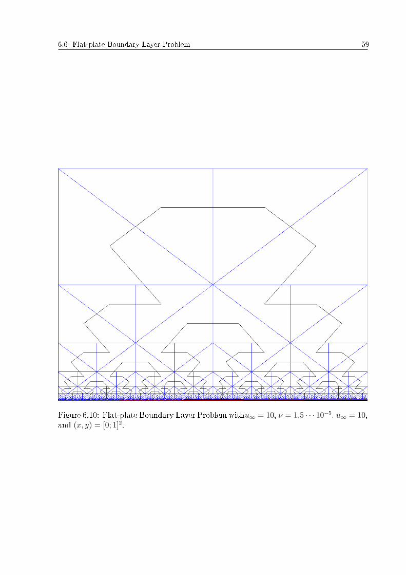
6.6 Flat-plate Boundary Layer Problem 59
Figure 6.10: Flat-plate Boundary Layer Problem withu∞ = 10, ν = 1.5 · · · 10−5, u∞ = 10,and (x, y) = [0; 1]2.

6.6 Flat-plate Boundary Layer Problem 60
Figure 6.11: Error of the numerical approximations to the at-plate Boundary LayerProblem with u∞ = 10, ν = 1.5 · · · 10−5, u∞ = 10, and (x, y) = [0; 1]2.
Therefore, a higher-order scheme should be applied in a future work. Figure 6.11 showsthe errors of the approximations with dierent levels of renement.
Finally, the total time (in seconds) spent in computations by a test presented in[Gonzaga, Guedes and Kischinhevsky, 2007] with 511 volumes was 8.75 · 10−1 and thetime spent in the renement process was2.1 ·10−2 (2.4%); whereas the total time spent incomputations by this present test with 521 volumes spent4.44 · 10−1 and the time spentin the renement process was 8.46 · 10−3 (1.82%).

Chapter 7
Conclusion
This work implements the Autonomous Leaves Graph (ALG) in a triangular discretizationbased on the Finite Volume Method for solving partial dierential equations (PDEs) withnon-uniform meshes through a cell-centered scheme. Triangular volumes may be moreecient to discretize complex domains than quadrangular volumes. The required datafor solving a PDE are stored in a graph data structure that performs the adaptive meshrenement (AMR). Original nodes in the local renement are not stored. This renementprocess allows that the created new pack from a single volume may be unrened, i.e. itmay return to a previous stage. This process intends to be as simple and straightforwardas the ALG original technique.
In addition, this scheme seeks to have low computational cost and exibility in order-ing the mesh and also linking neighbor volumes rened in dierent levels of renement incomparison with tree-based methods (quadtree and octree) and also the ALG technique.The mesh total-ordering scheme is performed by a Sierpi«ski-like Curve, which is imple-mented by means of a double-linked list. It is a non-regular version of the well-knowncurve due to the AMR. The renement and unrenement scheme of the triangular vol-ume enables straightforward update both in the linked list for mesh volume total orderingand graph nodes as well. Moreover, the Modied Hilbert Curve is more computationallyexpensive than the Sierpinski-like Curve.
Since this scheme yields a generalized sequential triangulation for total ordering, it isa triangular strip-like scheme. Besides, such sequential structure presents reduced connec-tivity information. Therefore, this scheme may be appropriate to be used in algorithmsthat generate triangle strip for accelerated rendering, algorithms that compute sequentialtriangulations for geometry compression and also in theoretical investigation of paths ontriangular meshes.
Additionally, in all tests accomplished, the linear systems presented sparse, symmetricand positive-denite coecient matrices. It is very likely that this scheme always produces

7 Conclusion 62
matrices with those properties and linear-system solvers based on the minimization offunctionals can be easily employed. Specically, the Conjugate Gradient Method wasemployed. Notice that no pre-conditioner was used.
These eciency results in much smaller memory requirements and larger savings incomputation times during the solution phase than tree-based schemes. The relative gainin eciency may be even more compelling for 3D problems. Since accessing the mainmemory of a computer system is currently a bottleneck in terms of performance, thosefeatures may be quite interesting.
Each problem is evaluated with its own features, and the most appropriate linearinterpolation must be employed for the problem. A specic linear integration is usedin order to construct the solution in respect to required gradients. This scheme maybe applied to either a simplied least-square gradient reconstruction or a vertex-centeredscheme. Moreover, the Median Dual scheme and Voronoi Diagrams (and its dual DelaunayTesselation) may be employed.
In the renement process, neither very large nor very small generated angles aredesirable. Thus, triangles are divided through successive bisections so that the anglesgenerated by the algorithm are necessarily bounded away from 0 andπ. Moreover, rstlyeach edge is divided into two equal parts, and, secondly, both triangles are bisected again.As a result, four new volumes with equal area are generated. Thus, this scheme intendsto present high-quality meshes during the renement process. This scheme intends toproduce graded and smoothed meshes. Namely, the area of neighboring triangles doesnot dramatically dier, though the scheme makes it possible through the graph datastructure. New studies may demonstrate that this approach may generate high-qualitymeshes during renement propagation even if the initial mesh does not present a qualitymesh. In addition, this scheme may be easily employed to the Finite Element Method.
Finally, although tests show only rectangular triangular volumes, any kind of trianglescan be used. Besides, this scheme can be extended to any polygonal volume shape.Furthermore, this technique enables any arbitrary polygonal shape for the initial domain,such as squares, rectangles, any kind of triangles and so on.
Tests showed numerical results in the Laplace (elliptic problem), Heat Conduction(parabolic problem), Wave (hyperbolic problem) Equations and at-plate Boundary LayerProblem.
Certainly, there is a lot of work yet to be done in this issue, including using thegraph data structure in moving meshes, implementing the 3D scheme, and in higher-order schemes, among others.
63
APPENDIX A -- Some historical descriptions
These historical descriptions can be mainly found in Wikipédia.
The word algebra is named after an Arabic word from the title of a book meaningThe book of Summary Concerning Calculating by Transposition and Reduction, a bookwritten by Abu Ja'far Muhammad ibn Musa al-Khwarizmi (about 790 - about 840), in820ac. The word Al-Jabr means reunion. On the other hand, Diophantus (between 200and 214 - between 284 and 290) has traditionally been known asthe father of algebra.
Abu Ja'far Muhammad ibn Musa al-Khwarizmi wrote a treatise in 825ac, On Cal-culation with Hindu Numerals, translated into Latin in the 12th century as Algoritmide numero indorum, which title was likely intended to mean Algoritmi on the numbersof the Indians, where Algoritmi was the rendition of the author's name; but peoplemisunderstanding the title led it to mean calculation method.
The Finite Element Methodoriginated from the need for solving complex elasticityand structural analysis problems in civil and aeronautical engineering. Its developmentcan be traced back to the work by Alexander Hrenniko (1896-1984) in 1941 and RichardCourant (1888-1972) in 1942. While the approaches used by these pioneers are dramati-cally dierent, they share one essential characteristic: mesh discretization of a continuousdomain into a set of discrete sub-domains, usually called elements. Hrenniko's workdiscretizes the domain by using a lattice analogy whereas Courant's approach divides thedomain into nite triangular subregions for solution of second order elliptic PDEs thatarise from the problem of torsion of a cylinder. Courant's contribution was evolutionary,drawing on a large body of earlier results for variational formulation of PDEs. Courantis also a namesake of the Courant minimax principle.
Hamiltonian triangulation is named after Willian Rowan Hamilton (1805-1865).His studies of mechanical and optical systems led him to discover far-reaching mathemat-ical concepts and techniques. His greatest contribution is perhaps the reformulation ofNewtonian mechanics, now called Hamiltonian mechanics, through the development ofaction principles and the eikonal function. This work has proven to be the central to themodern study of classical eld theories such as electromagnetism, and to the development

Appendix A -- Some historical descriptions 64
of quantum mechanics. In mathematics, he is perhaps best known for his discovery ofquaternions.
Isaac Newton (1642-1727) was a precursor in nite-dierences publishing a tract,Methodis dierentialis, in 1711, whereasMethodus incrementorum directa et inversa from1715 also qualies Brook Taylor (1685-1731) as one of the dierence-nite calculus founders.Isaac Newton's book, Philosophiæ Naturalis Principia Mathematica, published in 1687, isconsidered to be the most inuential one in the history of science. In this work, Newtondescribed universal gravitation and the three laws of motion, laying the groundwork forclassical mechanics, which dominated the scientic view of the physical Universe for thenext three centuries and is the basis for modern engineering. Newton showed that themotions of objects on Earth and of celestial bodies are governed by the same set of naturallaws by demonstrating the consistency between Kepler's laws of planetary motion and histheory of gravitation, thus removing the last doubts about heliocentrism and advancingthe scientic revolution. In mechanics, Newton enunciated the principles of conservationof momentum and angular momentum. In optics, he built the rst "practical" reectingtelescope and developed a theory of color based on the observation that a prism decom-poses white light into a visible spectrum. He also formulated an empirical law of coolingand studied the speed of sound. In mathematics, Newton shares the credit with GottfriedWilhelm Leibniz (1646-1716) for the development of the dierential and integral calculus.He also demonstrated the generalized binomial theorem, developed the so-called "New-ton's method" for approximating the zeroes of a function, and contributed to the studyof power series.
TheDivergence Theorem is an important result for the Mathematics of Physics, inparticular in Electrostatics and Fluid Dynamics. The theorem was rst stated by JosephLouis Lagrange (1736-1813) in 1762, then later described independently by Carl FriedrichGauss (1777-1855) in 1813, by George Green (1793-1841) in 1825 and in 1831 by MikhailVasilievich Ostrogradsky (1801-1862), who also provided the rst proof of the theorem.Born Giuseppe Lodovico Lagrangia, Lagrange made signicant contributions to analysis,to number theory, and to classical and celestial mechanics. Lagrange's treatise on ana-lytical mechanics (Mécanique Analytique, 4. ed., 2 vols. Paris: Gauthier-Villars et ls,1888-89), rst published in 1788, oered the most comprehensive treatment of classicalmechanics since Newton and formed a basis for the development of mathematical physics.Lagrange was one of the creators of the calculus of variations, deriving the Euler-Lagrangeequations for extrema of functionals. He also extended the method to take into accountpossible constraints, arriving at the method of Lagrange multipliers. Lagrange inventedthe method of solving dierential equations known as variation of parameters, applieddierential calculus to the theory of probabilities and attained notable work on the so-lution of equations. He proved that every natural number is a sum of four squares. His
Appendix A -- Some historical descriptions 65
treatise Theorie des fonctions analytiques laid some of the foundations of group theory.In calculus, Lagrange developed a novel approach to interpolation and Taylor series. Hestudied the three-body problem for the Earth, Sun, and Moon (1764) and the movementof Jupiter's satellites (1766), and in 1772 found the special-case solutions to this problemthat are now known as Lagrangian points. But above all he impressed on mechanics, hav-ing transformed Newtonian mechanics into a branch of analysis, Lagrangian mechanics asit is now called, and exhibited the so-called mechanical "principles" as simple results ofthe variational calculus. Ostrogradsky worked mainly in the mathematical elds of cal-culus of variations, integration of algebraic functions, number theory, algebra, geometry,probability theory and in the elds of mathematical physics and classical mechanics. Inthe latter his most important work includes researches of the motion of an elastic bodyand the development of methods for integration of the equations of dynamics.
The Green-Gauss technique is named after Green and Gauss. Gauss contributedsignicantly to many elds, including number theory, statistics, analysis, dierential ge-ometry, geodesy, electrostatics, astronomy, and optics. Green wroteAn Essay on theApplication of Mathematical Analysis to the Theories of Electricity and Magnetism in1828. The essay introduced several important concepts, among them a theorem similar tomodern Green's theorem, the idea of potential functions as currently used in physics, andthe concept of what are now called Green's functions. He was the rst to try to explain amathematical theory of the theories of electricity and magnetism which formed the basisfor other scientists.
The Cartesian coordinate system allowing geometric shapes to be expressed inalgebraic equations is named after René Descartes (1596-1650). He is accreditied as thefather of analytical geometry.
Voronoi Diagrams was proposed by Georgy Feodosevich Voronoi (1868-1908) in1907. He worked on continued fractions.
Dirichlet Tesselation is named after Johan Peter Gustav Lejeune Dirichlet (1805-1859), credited with the modern "formal" denition of a function.
Delaunay Tesselation, proposed in 1934, is named after Boris Nikolaevich Delone(1890-1980). He worked in the elds of modern algebra, the geometry of numbers. He alsoworked in the modern mathematical crystallography and general mathematical model ofcrystals.
Euler Equation is named after Leonhard Paul Euler (1707-1783). Euler made im-portant discoveries in elds as diverse as calculus and graph theory. He also introducedmuch of the modern mathematical terminology and notation, particularly for mathemat-ical analysis, such as the notion of a mathematical function. He is also renowned for his
Appendix A -- Some historical descriptions 66
work in mechanics, optics, and astronomy.
Navier-Stokes Equations, central to uid mechanics, are named after Claude-LouisNavier (1785-1836) and George Gabriel Stokes (1819-1903). Navier formulated the generaltheory of elasticity in a mathematically usable form in 1821, making it available to theeld of construction with sucient accuracy for the rst time. In 1819 he succeededin determining the zero line of mechanical stress, and in 1826 he established the elasticmodulus as a property of materials independent of the second moment of area. Navier istherefore often considered to be the founder of modern structural analysis. Stokes madeimportant contributions to uid dynamics, optics, and mathematical physics (includingStokes' theorem).
The Courant-Friendrichs-Lewy (CFL) condition was rstly proposed in 1928by: Richard Courant (1888-1972), who is attached to the Finite Element Method; KurtFriedrichs (1901-1982), who greatest contribution was his work on PDEs and; Hans Lewy(1904-1988), who was also known for his work on PDEs.
Euclidian space is named after Euclid of Alexandria (about 325bc - about 265bc).He is often referred to as the Father of Geometry. His workElements is the most suc-cessful textbook in the history of mathematics. In it, the principles of what is now calledEuclidean geometry were deduced from a small set of axioms. Euclid also wrote works onperspective, conic sections, spherical geometry, number theory and rigor.
Discrete Boltzmann Equation is named after Ludwig Eduard Boltzmann (1844-1906). He is famous for his founding contributions in the elds of statistical mechanicsand statistical thermodynamics. He was one of the most important advocates for atomictheory when that scientic model was still highly controversial.
Generalized Riemann Problems are named after Georg Friedrich Bernhard Rie-mann (1826-1866). He gave fundamental contributions to the dierential analysis andgeometry, which some opened a path to the development of the general relativity. Hisname is linked to Riemann Zeta function, Riemann Lemma, Rieman Fold and the Rie-mann surfaces.
Taylor-series expansion are named after Brook Taylor (1685-1731). He obtaineda remarkable solution of the problem of the "centre of oscillation", published in 1714.Taylor's Methodus Incrementorum Directa et Inversa (1715) added a new branch to thehigher mathematics, now designated the "calculus of nite dierences". He used it todetermine the form of movement of a vibrating string, by him rst successfully reduced tomechanical principles. The same work contained the celebrated formula known as Taylor'stheorem, the importance of which remained unrecognized until 1772, when J. L. Lagrangerealized its powers and termed it le principal fondement du calcul diérentiel. In his 1715

Appendix A -- Some historical descriptions 67
essay Linear Perspective, Taylor set forth the true principles of the art in an original andmore general form than any of his predecessors; but the work suered from the brevityand obscurity which aected most of his writings.
The upwind scheme was rst proposed, in 1952, by Richard Courant (1888-1972),Eugene Isaacson (1919-2008), one of the pioneers of modern numerical mathematics, andMina Spiegel Rees (1902-1997), who worked in Applied Mathematics.
In 1887, Marie Ennemond Camille Jordan (1838-1922) introduced a rigorous deni-tion, since adopted a precise description, of the continuous curve notion. He is knownboth for his foundational work in group theory and for his inuentialCours d'analyse.
Space-lling curves or Peano Curves are curves, rst described by Giuseppe Peano(1858-1932) in 1880, whose ranges contain the entire 2D unit square (or the 3D unit cube).He was author of over 200 books and papers. He was a founder of mathematical logic andset theory, to which he contributed with much notation. The standard axiomatizationof the natural numbers is named in his honor. As part of this axiomatization eort, hemade key contributions to the modern rigorous and systematic treatment of the methodof mathematical induction.
Wacªaw Franciszek Sierpi«ski (1882-1969) was known for outstanding contributions toset theory (research on the axiom of choice and the continuum hypothesis), number theory,theory of functions and topology. He published over 700 papers and 50 books. Three well-known fractals are named after him (the Sierpi«ski triangle, the Sierpi«ski carpet and theSierpi«ski curve), as are Sierpi«ski numbers and the associated Sierpi«ski problem.
Jacques Salomon Hadamard (1865-1963) was known for his proof of the prime numbertheorem in 1896. He introduced the idea ofwell-posed problem in the theory of partialdierential equations. He also gave his name to the Hadamard inequality on volumes,and the Hadamard matrix, on which the Hadamard transform is based. The Hadamardgate in quantum computing uses this matrix.
David Hilbert (1862-1943) proposed the Hilbert Curve, a space-lling curve, in1891. He is recognized as one of the most inuential and universal mathematicians of the19th and early 20th centuries. He invented or developed a broad range of fundamentalideas in many areas, including invariant theory and the axiomatization of geometry. Healso formulated the theory of Hilbert spaces, one of the foundations of functional anal-ysis. Hilbert adopted and warmly defended the set theory and transnite numbers. Afamous example of his leadership in mathematics is his 1900 presentation of a collection ofproblems that set the course for much of the mathematical research of the 20th century.Hilbert and his students supplied signicant portions of the mathematical infrastructurerequired for quantum mechanics and general relativity. He is also known as one of the

Appendix A -- Some historical descriptions 68
founders of proof theory, mathematical logic and the distinction between mathematicsand metamathematics.
Boundary layers have been of great importance in the study of viscous uid ow.In 1904, Ludwig Prandtl (1875-1953) demonstrated the existence of a thin boundary layerin uid ow. Moreover, he found that there exists a thin layer near an object surface,where the viscous aerodynamic forces are as important as the inertial forces. He wasa pioneer of aerodynamics, and developed the mathematical basis for the fundamentalprinciples of subsonic aerodynamics in the 1920s. His studies identied the boundarylayer, thin-airfoils, and lifting-line theories. The Prandtl number was named after him.
Blasius Solution is named after Paul Richard Heinrich Blasius (1883-1970). Oneof his contributions involves a description of the steady two-dimensional boundary-layerthat forms on a semi-innite plate which is held parallel to a constant unidirectional ow.
Reynolds number is named after Osborne Reynolds (1842-1912). He was a promi-nent innovator in the understanding of uid dynamics. Separately, his studies of heattransfer between solids and uids brought improvements in boiler and condenser design.
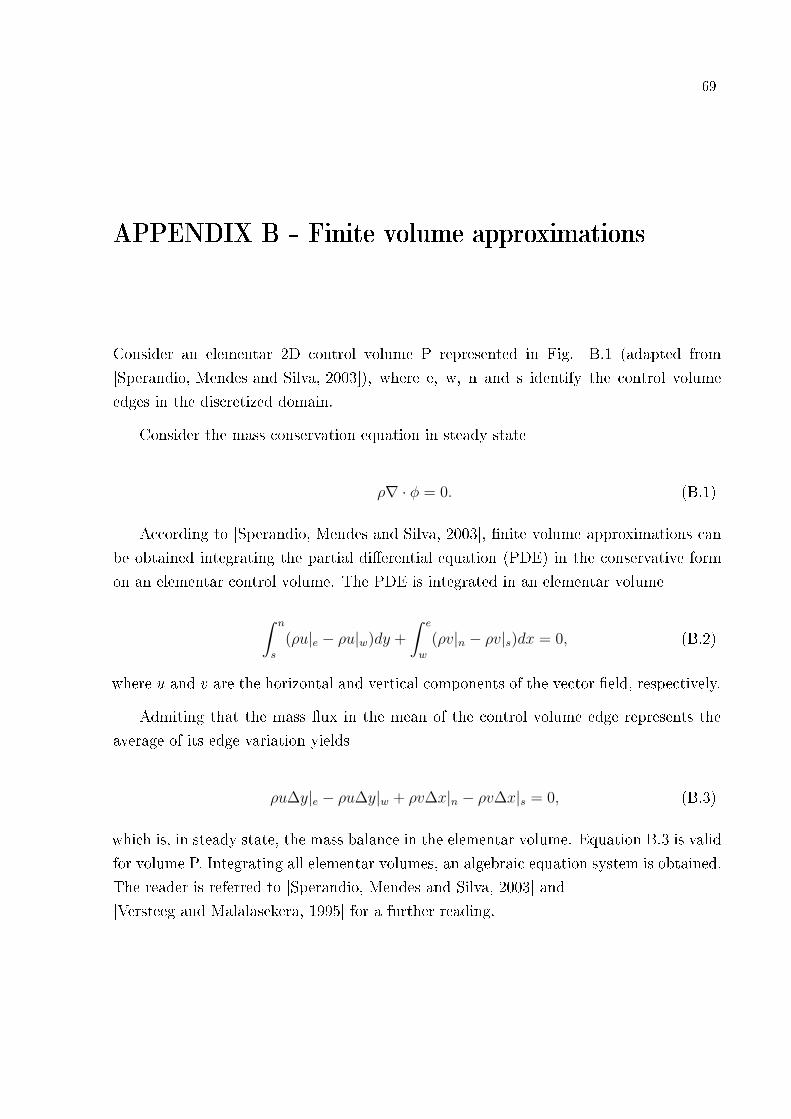
69
APPENDIX B -- Finite volume approximations
Consider an elementar 2D control volume P represented in Fig. B.1 (adapted from[Sperandio, Mendes and Silva, 2003]), where e, w, n and s identify the control volumeedges in the discretized domain.
Consider the mass conservation equation in steady state
ρ∇ · φ = 0. (B.1)
According to [Sperandio, Mendes and Silva, 2003], nite volume approximations canbe obtained integrating the partial dierential equation (PDE) in the conservative formon an elementar control volume. The PDE is integrated in an elementar volume
∫ n
s
(ρu|e − ρu|w)dy +
∫ e
w
(ρv|n − ρv|s)dx = 0, (B.2)
where u and v are the horizontal and vertical components of the vector eld, respectively.
Admiting that the mass ux in the mean of the control volume edge represents theaverage of its edge variation yields
ρu∆y|e − ρu∆y|w + ρv∆x|n − ρv∆x|s = 0, (B.3)
which is, in steady state, the mass balance in the elementar volume. Equation B.3 is validfor volume P. Integrating all elementar volumes, an algebraic equation system is obtained.The reader is referred to [Sperandio, Mendes and Silva, 2003] and[Versteeg and Malalasekera, 1995] for a further reading.

Appendix B -- Finite volume approximations 70
Figure B.1: Elementar 2D control volume.

71
APPENDIX C -- A mathematical proof by induction
Theorem : [∀n ∈ N|n even ∧ 2n =2
n2∑
i=1
(2i− 1)] (C.1)
The theorem C.1 states that for alln natural even, 2n is the sum of odd numbers from1 to 2
n2 .
20 = 1
22 = 1 + 3
24 = 1 + 3 + 5 + 7
26 = 1 + 3 + 5 + 7 + 9 + 11 + 13 + 15
28 = 1 + 3 + 5 + 7 + 9 + 11 + 13 + 15 + . . . + 31
. . .
2n =2
n2∑
i=1
(2i− 1).
Proof: for this demonstration, the induction basis is
P (0) : 20 = 1 (C.2)
orP (2) : 22 = 1 + 3. (C.3)
The inductive hypothesis is
P (k) : 2k =2
k2∑
i=1
(2i− 1). (C.4)
The inductive step is
P (k + 2) : 2k+2 ?=
2·2 k2∑
i=1
(2i− 1) (C.5)

Appendix C -- A mathematical proof by induction 72
or
P (k + 2) : 4 · 2k ?= 4 ·
2k2∑
i=1
(2i− 1)
︸ ︷︷ ︸2k
HI=
2·2k2∑
i=1
(2i− 1)
︸ ︷︷ ︸4·2k?
. (C.6)
The righ-hand side summation of C.6 can be decomposed in
2k2 +1∑i=1
(2i− 1) =2
k2∑
i=1
(2i− 1)
︸ ︷︷ ︸2k
+2
k2 +1∑
i=2k2 +1
(2i− 1)
︸ ︷︷ ︸3·2k?
. (C.7)
By the inductive hypothesis, C.4 is assumed true. Then, the rst summation on right-hand side of C.7 is 2k. Thus, the second summation on right-hand side of C.7 must beveried if it is equal to 3 · 2k.
One can dene
Lemma : [∀n ∈ N∗|n even ∧ 2n =
2n2 +1∑
i=2n2 +1
(2i− 1)
3]. (C.8)
Proof: for the sum2·2 k
2∑
i=2k2 +1
(2i− 1)
︸ ︷︷ ︸3·2k?
, a variable transformation from i to j is performed
j = i− 2k2 . (C.9)
Thus,i = j + 2
k2 . (C.10)
For the initial limit of the summation in j
j = 2k2 + 1− 2
k2 = 1. (C.11)
For the nal limit of the summation in j
j = 2 · 2 k2 − 2
k2 = 2
k2 . (C.12)
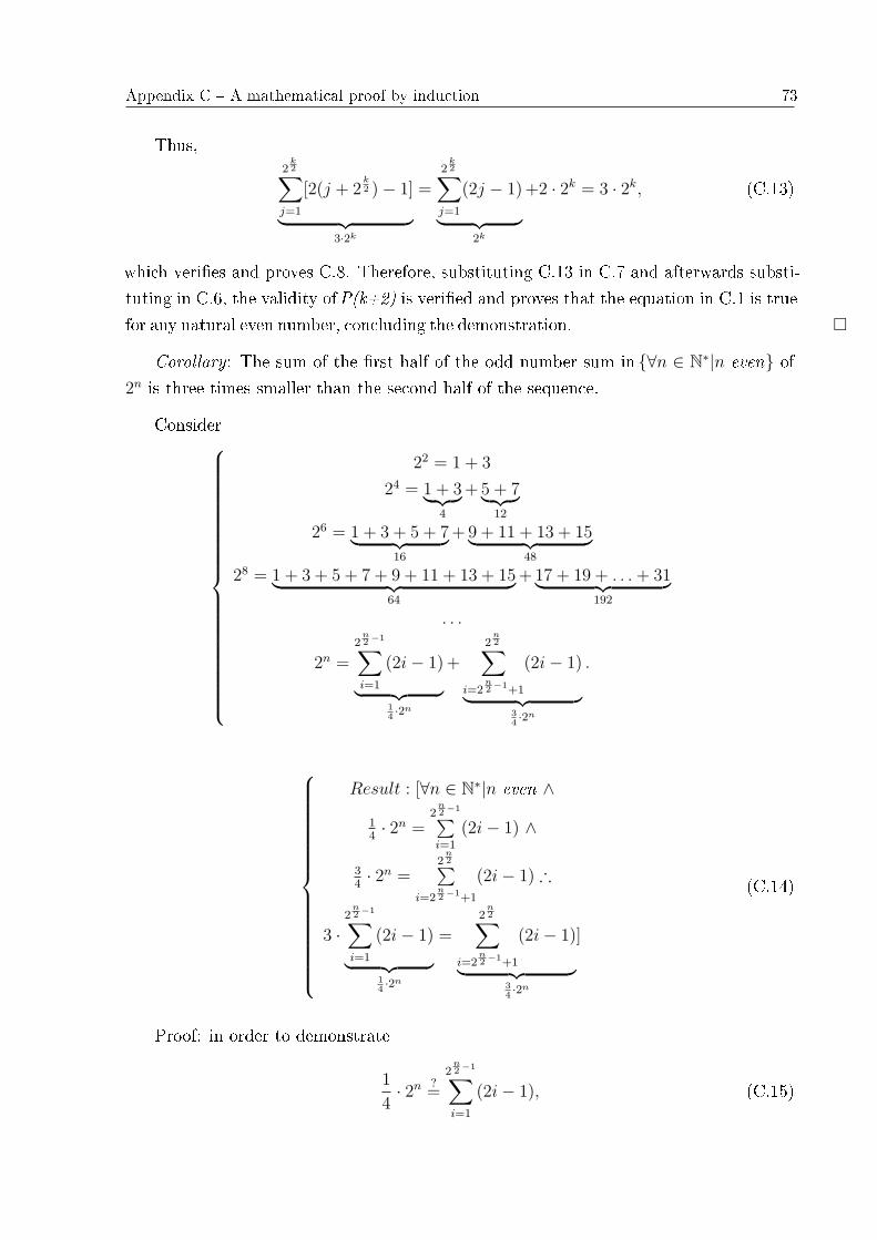
Appendix C -- A mathematical proof by induction 73
Thus,2
k2∑
j=1
[2(j + 2k2 )− 1]
︸ ︷︷ ︸3·2k
=2
k2∑
j=1
(2j − 1)
︸ ︷︷ ︸2k
+2 · 2k = 3 · 2k, (C.13)
which veries and proves C.8. Therefore, substituting C.13 in C.7 and afterwards substi-tuting in C.6, the validity ofP(k+2) is veried and proves that the equation in C.1 is truefor any natural even number, concluding the demonstration. ¤
Corollary: The sum of the rst half of the odd number sum in ∀n ∈ N∗|n even of2n is three times smaller than the second half of the sequence.
Consider
22 = 1 + 3
24 = 1 + 3︸ ︷︷ ︸4
+ 5 + 7︸ ︷︷ ︸12
26 = 1 + 3 + 5 + 7︸ ︷︷ ︸16
+ 9 + 11 + 13 + 15︸ ︷︷ ︸48
28 = 1 + 3 + 5 + 7 + 9 + 11 + 13 + 15︸ ︷︷ ︸64
+ 17 + 19 + . . . + 31︸ ︷︷ ︸192
. . .
2n =2
n2−1∑i=1
(2i− 1)
︸ ︷︷ ︸14·2n
+2
n2∑
i=2n2−1+1
(2i− 1)
︸ ︷︷ ︸34·2n
.
Result : [∀n ∈ N∗|n even ∧14· 2n =
2n2−1∑i=1
(2i− 1) ∧
34· 2n =
2n2∑
i=2n2−1+1
(2i− 1) ∴
3 ·2
n2−1∑i=1
(2i− 1)
︸ ︷︷ ︸14·2n
=2
n2∑
i=2n2−1+1
(2i− 1)
︸ ︷︷ ︸34·2n
]
(C.14)
Proof: in order to demonstrate
1
4· 2n ?
=2
n2−1∑i=1
(2i− 1), (C.15)

Appendix C -- A mathematical proof by induction 74
the basis induction is
P (2) :1
4· 22 =
222−1∑i=1
(2i− 1) = 1. (C.16)
The inductive hypothesis is
P (k) :1
4· 2k =
2k2−1∑i=1
(2i− 1). (C.17)
One must verify if
1
4· 2k ?
=1
4·
2k2∑
i=1
(2i− 1)
︸ ︷︷ ︸2n
= 2−2 ·2
k2∑
i=1
(2i− 1)
︸ ︷︷ ︸2n
(C.18)
or
2k−2 HI=
2k2−1∑i=1
(2i− 1)
︸ ︷︷ ︸14·2n?
. (C.19)
The inductive step
P (k + 2) : 2k−2+2 ?=
2·2 k2−1∑
i=1
(2i− 1) =2
k2−1+1∑i=1
(2i− 1) (C.20)
is the theorem C.1 already proved: 2n =2
n2∑
i=1
(2i− 1). Consequently, it proves that C.15 istrue.
In order to prove 34· 2n =
2n2∑
i=2n2−1+1
(2i − 1), a variable transformation from i to j is
performedj = i− 2
k2−1. (C.21)
Thus,i = j + 2
k2−1. (C.22)
For the initial limite of the summation in j
j = 2k2−1 + 1− 2
k2−1 = 1. (C.23)

Appendix C -- A mathematical proof by induction 75
For the nal limit of the summation in j
j = 2k2 − 1
2· 2 k
2 = 2k2−1. (C.24)
Thus,
2k2−1∑
j=1
[2(j + 2k2−1)− 1] =
2k2−1∑
j=1
(2j − 1)
︸ ︷︷ ︸14·2k
+ 2 · (2−1 · 2 k2 ) · (2 k
2 · 2−1)︸ ︷︷ ︸(2·2−1)·2k · 2−1︸ ︷︷ ︸
24 ·2k
=3
4· 2k, (C.25)
which veries and proves that C.14 is true, concluding the demonstration. ¤

76
APPENDIX D -- Remarks for 3D
This scheme allows tetrahedral volumes to be straightforwardly rened and ordered. Fig-ure D.1 sketches a tetrahedral volume and its faces highlighted. A tetrahedral volumepresents 12 external angles (three angles for each four faces).
Figure D.2 sketches a tetrahedral renement. Similarly to the 2D case, the largestedge (of the largest face) is chosen for renement. Assume that the face with the largestarea is ACD and the edge AD is the longest-edge of the tetrahedral shown in Fig. D.2a.Locating the mean point E of the edge AD, the medians BE and CE are traced.
The triangular face BCE divides the tetrahedral in two new ones which each one hasthe half-volume of the original tetrahedral. Figures D.2b-d display the two new tetrahedra.Figures D.2e-g depict both tetrahedra divided a second time. The four new tetrahedrapresents each one the fourth-volume of the original tetrahedral.
This scheme is similar to the 4-triangles largest side partition of the largest faceACD, where point E is the mean point of the largest edge. This is followed by tracing themedians of the three remaining faces: BE, BF and BG, since the vertexB is the oppositevertex of mean points E, F and G in the faces ABD, ABC and BCD, respectively.
Figure D.3a sketches three tetrahedral volumesABCD, ABCF and BCFG, which
Figure D.1: (a) Tetrahedral volume with view from top; (b) detail of the front face view;(c) detail of the left front face view; (d) detail of the background face and; (e) detail ofthe right face.

Appendix D -- Remarks for 3D 77
Figure D.2: (a) original tetrahedral; (b) new tetrahedral, which is in the back; (c) newtetrahedral, which is in front; (d) both new tetrahedral uncoupled; (e) four new tetrahe-dral; (f) rst two tetrahedra and (g) last two tetrahedra.
Figure D.3: (a) Three tetrahedral volumes (GFBC, FACB and CBAD); (b) renementof the front left tetrahedral volume into two new ones where black points indicate thetetrahedral volume centroids and there is a curve representing the 3D Sierpi«ski-likeCurve as well as lines indicating median lines of the background of tetrahedral volumes.
are linked by a 3D Sierpi«ski-like Curve. The tetrahedral volume on left is rened andthe 3D Sierpi«ski-like Curve is updated in Fig. D.3b. Each new tetrahedral has thehalf-volume of the original tetrahedral. As a simple example, it is parted in just twotetrahedra and the new partition of both could follow the scheme shown. Solution of thisscheme should follow the Frink's reconstruction [Frink, Parikh and Pirzadeh, 1991].
Bibliography
[Anderson, Tannehill and Pletcher, 1984]ANDERSON, D. A.; TANNEHILL, J. C.;PLETCHER, R. H. Computational Fluid Mechanics and Heat Transfer: Hemisphere,1984.
[Arkin et al., 1994]ARKIN, E.; HELD, M.; MITCHEL, J.; SKIENA, S. Hamiltonian tri-angulations for fast rendering. The 2nd Annual European Symposium on Algorithms,(LNCS), v. 855, p. 3647, . Springer, Berlin Heidelberg New York 1994.
[Arnold, 2001]ARNOLD, D. N. A Concise Introduction to Numerical Analysis:http://www.ima.umn.edu/ arnold/, 2001.
[Azevedo and Korzenowsk, 1999]AZEVEDO, L. F. F. da Silvaand João L. F.; KO-RZENOWSK, H. On the development of an unstructured grid solver for inert and reac-tive high speed ow simulations. J. Braz. Soc. Mech. Sci., v. 21, n. 4, 1999.
[Baliga and Patankar, 1980]BALIGA, B.; PATANKAR, S. V. A new nite element for-mulation for convection diusion problems.Numerical Heat Transfer, v. 3, p. 393409,1980.
[Barth, 1993]BARTH, T. J. Recent developments in high order k-exact reconstruction onunstructured meshes. 31st Aerospace Sciences Meeting and Exhibit, January 1993.
[Barth, 1994]BARTH, T. J.Aspects of unstructured grids and nite-volume solvers for theEuler and Navier-Stokes Equations: VKI Lecture Series, 1994.
[Barth and Ohlberger, 2004]BARTH, T. J.; OHLBERGER, M.Finite Volume Methods:foundation and analysis: John Wiley and Sons, 2004.
[Berger, Aftosmis and Melton, 1998]BERGER, M. J.; AFTOSMIS, M.; MELTON, J. Ac-curacy, adaptive methods and complex geometry. Proc. First AFOSR Conference onDynamic Motion CFD, 1998.
[Berger, Helzel and LeVeque, 2003]BERGER, M. J.; HELZEL, C.; LEVEQUE, R. J.H -box methods for the approximation of hyperbolic conservation laws on irregular grids.SIAM Journal on Numerical Analysis, v. 41, n. 3, p. 893918, 2003.

BIBLIOGRAPHY 79
[Bertolazzi and Manzini, 2008]BERTOLAZZI, E.; MANZINI, G. Polynomialreconstructions and limiting strategies in nite volume approximations:http://historical.ncstrl.org/tr/fulltext/tr/ercimcnr/2002-1289.txt, 2008.
[Bouche, Ghidaglia and Pascal, 2005]BOUCHE, D.; GHIDAGLIA, J.-M.; PASCAL, F.Error estimate and the geometric corrector for the upwind Finite Volume Method appliedto the linear advection equation. SIAM J. Numer. Anal., v. 43, n. 2, p. 578603, 2005.
[Bramkamp, Ballmann and Muller, 2000]BRAMKAMP, F.; BALLMANN, J.; MULLER,S. Development of a ow solver employing local adaptation based on multiscale analysison b-spline grids. Proceedings of 8th Annual Conf. of the CFD Society of Canada, June2000.
[Bramkamp et al., 2003]BRAMKAMP, F. et al. H-adaptive multiscale schemes for thecompressible Navier-Stokes Equations - polyhedral discretization, data compression andmesh generation. Numerical Notes on Fluid Mechanics, v. 84, p. 125204, 2003.
[Bramkamp, Lamby and Muller, 2004]BRAMKAMP, F.; LAMBY, P.; MULLER, S. Anadaptive multiscale nite volume solver for unsteady and steady state ow computations.Journal of Computational Physics, v. 197, p. 460490, 2004.
[Brandao, Gonzaga and Kischinhevsky, 2008]BRANDAO, D. N.; GONZAGA, S. L. deO.; KISCHINHEVSKY, M. Finite element h-adaptive renement procedure based onautonomous leaves graph.XXIX CILAMCE - Iberian Latin American Congress on Com-putational Methods in Engineering, November 2008.
[Brandao, Gonzaga and Kischinhevsky, 2009]BRANDAO, D. N.; GONZAGA, S. L. deO.; KISCHINHEVSKY, M. Finite-element non-conforming h-adaptivity strategy basedon autonomous leaves graph (to appear). International Conference on ComputationalScience. LNCS,, May 2009.
[Burgarelli, Kischinhevsky and Biezuner, 2006]BURGARELLI, D. D.; KISCHIN-HEVSKY, M.; BIEZUNER, R. J. A new adaptive mesh renement strategy fornumerically solving evolutionary PDE's. Journal of Computational and AppliedMathematics, v. 196, p. 115131, 2006.
[Carpenter et al., 1989]CARPENTER, R. L. J.; DROEGEMEIER, K. K.; WOODWARD,P. R.; HANE, C. E. Application of the piecewise parabolic method (PPM) to metereo-logical modeling. Monthly Weather Review, v. 118, p. 586612, 1989.
[Colella and Woodward, 1984]COLELLA, P.; WOODWARD, P. R. The piecewiseparabolic method (PPM) for gas-dynamical simulations. Journal of ComputationalPhysics, v. 54, p. 174201, 1984.

BIBLIOGRAPHY 80
[Cormen et al., 2001]CORMEN, T. H.; LEISERSON, C. E.; RIVEST, R. L.; STEIN, C.Introduction to Algorithms: McGraw-Hill Book Company, 2001.
[Douglas and Russel, 1982]DOUGLAS, J.; RUSSEL, T. Diusion problems on combiningthe method of characteristics with nite element or nite dierence procedures.SIAMJ. Numer. Anal., v. 19, p. 871885, 1982.
[Fonseca, 2005]FONSECA, L. C. M. da. Estudo comparativo de esquemas para o cálculode trajetórias no método semi-lagrangeano: Dissertation, Universidade Federal do Riode Janeiro, 2005.
[Frink, 1994]FRINK, N. T. Recent progress toward a three-dimensional unstructuredNavier-Stokes ow solver. 32nd Aerospace Sciences Meeting, n. 0061, January 1994.
[Frink, 1996]FRINK, N. T. Assessment of an unstructured-grid method for predicting 3-Dturbulent viscous ows. 34th Aerospace Sciences Meeting, n. 0292, January 1996.
[Frink, Parikh and Pirzadeh, 1991]FRINK, N. T.; PARIKH, P.; PIRZADEH, S. A fastupwind solver for the Euler Equations on three-dimensional unstructured meshes.AIAA,n. 0102, 1991.
[Furst, 2006]FURST, J. A weighted least square scheme for compressible ows.AppliedScientic Research, v. 76, n. 4, p. 331342, June 2006.
[Galante, 2006]GALANTE, G. Métodos Multigrid Paralelos Aplicados à Simulação deProblemas de Dinâmica de Fluidos Computacional: Universidade Federal do Rio Grandedo Sul, 2006.
[Gonzaga, Guedes and Kischinhevsky, 2007]GONZAGA, S. L. de O.; GUEDES, M.;KISCHINHEVSKY, M. Método dos Volumes Finitos com renamento adaptativo demalhas aplicado ao problema da camada limite.XXIIX CILAMCE - Iberian Latin Amer-ican Congress on Computational Methods in Engineering, June 2007.
[Gonzaga and Kischinhevsky, 2008]GONZAGA, S. L. de O.; KISCHINHEVSKY, M. Sier-pinski curve for total ordering of a graph-based adaptive simplicial-mesh renement fornite volume discretizations.XXXI CNMAC - Congresso Nacional de Matemática Apli-cada e Computacional, September 2008.
[Gonzaga and Kischinhevsky, 2009]GONZAGA, S. L. de O.; KISCHINHEVSKY, M. Au-tonomous leaves graph applied to the boundary layer problem (to appear).InternationalConference on Computational Science. LNCS,, May 2009.

BIBLIOGRAPHY 81
[Gonzaga et al., 2008]GONZAGA, S. L. de O.; KISCHINHEVSKY, M.; BURGARELLI,D. D.; BIEZUNER, R. Graph-based adaptive simplicial-mesh renement for nite vol-ume discretizations. XXIX CILAMCE - Iberian Latin American Congress on Computa-tional Methods in Engineering, October 2008.
[Guibas and Stol, 1985]GUIBAS, L.; STOLFI, J. Primitives for the manipulation ofgeneral subdivisions and the computation of Voronoi Diagrams.ACM Transactions onGraphics, v. 4, n. 2, p. 74123, 1985.
[Harten, 1983]HARTEN, A. High resolution schemes for hyperbolic conservation laws.J.Comput. Phys., v. 49, n. 197, p. 357293, 1983.
[Helzel, Berger and LeVeque, 2005]HELZEL, C.; BERGER, M. J.; LEVEQUE, R. J. Ahigh-resolution rotated grid method for conservation laws with embedded geometries.SIAM Journal on Scientic Computing, v. 26, n. 3, p. 785809, 2005.
[Hestenes and Stiefel, 1952]HESTENES, M. R.; STIEFEL, E. L. Methods of conjugategradients for solving linear systems. J.Res.Nat.Bur.Stand., v. 49, p. 409436, 1952.
[Iaccarino and Ham, 2004]IACCARINO, G.; HAM, F. Automatic mesh generation for lesin complex geometries. Annual Research Briefs 2005 - Center for Turbulence Research,v. 197, p. 460490, 2004.
[Iske and Kaser, 2004]ISKE, A.; KASER, M. Conservative semi-lagrangian advection onadaptive unstructured meshes. Numer. Meth. Par. Di. Eq., v. 20, n. 3, p. 388411,2004.
[Jeon and Sheen, 2005]JEON, Y.; SHEEN, D. Analysis of a cell Boundary ElementMethod. Advances in Computational Mathematics, v. 22, p. 201222, 2005.
[Jones and Plassmann, 1997]JONES, M.; PLASSMANN, P. Adaptive renement of un-structured nite-element meshes. Journal of Finite Elements in Analysis and Design,v. 25, n. 1-2, p. 4160, 1997.
[Ju, 2004]JU, L. Conforming centroidal Voronoi Delaunay triangulation for quality meshgeneration. International Journal of Numerical Analysis and Modeling, v. 1, n. 1, p.117, 2004.
[Kaser and Iske, 2005]KASER, M.; ISKE, A. Ader schemes on adaptive triangular meshesfor scalar conservation laws. Journal of Computational Physics, v. 205, p. 486508, 2005.
[Kim and Choi, 2000]KIM, D.; CHOI, H. A second-order time-accurate Finite VolumeMethod for unsteady incompressible ow on hybrid unstructured grids.Journal of Com-putational Physics, v. 162, p. 411428, 2000.
BIBLIOGRAPHY 82
[Kobayashi, Pereira and Pereira, 1999]KOBAYASHI, M.; PEREIRA, J.; PEREIRA, J. Aconservative nite-volume second-order-accurate projection method on hybrid unstruc-tured grids. Journal of Computational Physics, v. 150, p. 4075, 1999.
[Leithold, 1994]LEITHOLD, L. O cálculo com Geometria Analítica (3a. ed.): EditoraHarbra, 1994.
[Madsen, 1998]MADSEN, J.Design optimization of internal ow devices. Thesis (Ph.D.),1998.
[Márquez et al., 2008]MÁRQUEZ, A.; MORENO-GONZÁLEZ, A.; PLAZA, A.;SUÁREZ, J. P. The seven-triangle longest-side partition of triangles and mesh qual-ity improvement. Finite Elements in Analysis and Design, v. 44, p. 748758, July 2008.
[Mathur and Murthy, 1997]MATHUR, S.; MURTHY, J. A pressure based method forunstructured meshes. Numerical Heat Transfer part B, v. 31, p. 195215, 1997.
[McManus et al., 2000]MCMANUS, K. et al. A scalable strategy for the paralelizationof multiphysics unstructured mesh-iterative codes on distributed-memory systems.TheInternational Journal of High Performance Computing Applications, v. 4, n. 14, p. 137174, 2000.
[Moura, 2002]MOURA, C. A. Análise Funcional para aplicações - Posologia: EditoraCiência Moderna, 2002.
[Neel, 1997]NEEL, R. Advances in computational uid dynamics: turbulent separatedows and transonic potential ows: Dissertation, Faculty of Virginia Polytechnic In-stitute and State University, 1997.
[Northrup, 2004]NORTHRUP, S. A. A Parallel Adaptive-Mesh Renement Scheme forPredicting Laminar Diusion Flames: Dissertation, University of Toronto, 2004.
[OpenGL, 1993]OPENGL, A. R. B.OpenGL Reference Manual: Addison Wesley, 1993.
[Ozawa and Tanahashi, 2005]OZAWA, T.; TANAHASHI, T. CIVA (Cubic Interpolationwith Volume/Area Coordinates) and AMR (Adaptive Mesh Renement) Method forDiscrete Boltzmann Equation. JSME International Journal, Series B, v. 48, n. 2, p.229234, 2005.
[Pandya and Frink, 2004]PANDYA, M. J.; FRINK, N. T. An agglomeration multigrid foran unstructured-grid ow solver. 42nd AIAA Aerospace Sciences Meeting and Exhibit,n. 0759, January 2004.
BIBLIOGRAPHY 83
[Pantano et al., 2007]PANTANO, C.; DEITERDING, R.; HILL, D.; PULLIN, D. A lownumerical dissipation patch-based adaptive mesh renement method for large-eddy sim-ulation of compressible ows. Journal of Computational Physics, v. 221, p. 6387, 2007.
[Pascal and Ghidaglia, 2001]PASCAL, F.; GHIDAGLIA, J.-M. Footbridges between nitevolumes and nite elements with applications to CFD.Int. J. for Numer. Meth. in Fluids,v. 37, p. 951986, 2001.
[Rivara, 1984a]RIVARA, M. C. Design and data structure of fully adaptive, multigrid,nite-element software. ACM Transactions on Mathematical Software, v. 10, n. 3, p.242264, September 1984a.
[Rivara, 1984b]RIVARA, M. C. Algorithms for rening triangular grids suitable for adap-tive and multigrid techniques. Int. J. for Num. Meth. in Eng., v. 20, p. 745756, 1984b.
[Rivara, 1984c]RIVARA, M. C. Mesh renement processes based on the generalized bi-section of simplices. SIAM Journal on Numerical Analysis, v. 21, n. 3, p. 604613, June1984c.
[Rivara and Iribarren, 1996]RIVARA, M. C.; IRIBARREN, G. The 4-triangles longest-side partition of triangles and linear renement algorithms.Mathematics of Computation,v. 65, n. 216, p. 14851502, November 1996.
[Sachdev, Groth and Gottlieb, 2005]SACHDEV, J.; GROTH, C.; GOTTLIEB, J. ParallelAMR scheme for turbulent multi-phase rocket motor core ows.17th AIAA Computa-tional Fluid Dynamics Conference, n. 5334, p. 69, June 2005.
[Schlichting, 1979]SCHLICHTING, H.Boundary-Layer Theory: McGraw-Hill Inc., 1979.
[Schneider and Maliska, 2002]SCHNEIDER, F. A.; MALISKA, C. R. Solução numérica deproblemas convectivos-difusivos bidimensionais pelo Método dos Volumes Finitos usandomalhas não estruturadas. IX Congresso Brasileiro de Engenharias e Ciências Térmicas,n. 0346, 2002.
[Schneider and Raw, 1987]SCHNEIDER, G.; RAW, M. Control volume Finite ElementMethod for heat transfer and uid ow using co-located variables 2: Application andvalidation. Numerical Heat Transfer, v. 11, p. 391400, 1987.
[Shewchuk, 1999]SHEWCHUK, J. R.Lecture Notes on Delaunay Mesh Generation: Uni-versity of California at Berkeley, 1999.
[Sierpi«ski, 1912]SIERPISKI, W. Sur une nouvelle courbe continue qui remplit touteune aire plane. Bull. l'Acad. des Sciences Cracovie A, p. 462478, 1912.
BIBLIOGRAPHY 84
[Sierpi«ski, 1916]SIERPISKI, W. Sur une courbe cantorienne qui contient une imagebiunivoque et continue de toute courbe donee. Comptes Rendus Acad. Sci., v. 162, p.629632, 1916.
[Speckmann and Snoeyink, 1997]SPECKMANN, B.; SNOEYINK, J. Easy triangle stripsfor TIN terrain models. Canadian Conference on Computational Geometry, p. 239244,1997.
[Sperandio, Mendes and Silva, 2003]SPERANDIO, D.; MENDES, J. ao T.; SILVA, L.H. M. e. Cálculo Numérico: Características Matemáticas e Computacionais dos MétodosNuméricos: Pearson Prentice Hall, 2003.
[Stynes, 1980]STYNES, M. On faster convergence of the bisection method for all triangles.Mathematics of Computation, v. 35, n. 152, p. 11951201, October 1980.
[Tanaka, 1999]TANAKA, N. Development of a highly accurate interpolation method formesh-free ow simulations i. integration of gridless, particle and CIP methods.J. Numer.Methods Fluids, v. 30, n. 8, p. 957976, 1999.
[Tanaka, Yamasaki and Tagushi, 2004]TANAKA, N.; YAMASAKI, T.; TAGUSHI, T. Ac-curate and robust uid analysis using cubic interpolation with volume/area coordinates(CIVA) method on unstructured grids. JSME International Journal, Series B, v. 47,n. 4, p. 672680, 2004.
[Turner and Ferguson, 1995]TURNER, I.; FERGUSON, W. An unstructured mesh cell-centered control volume method for simulating heat and mass transfer in porous media:application to softwood drying-part ii: the anisotropic model.Appl. Math. Modeling,v. 19, p. 668674, 1995.
[Velho, Figueiredo and Gomes, 1999]VELHO, L.; FIGUEIREDO, L. H. de; GOMES, J.Hierarchical generalized triangle strips.The Visual Computer, v. 15, p. 2135, 1999.
[Versteeg and Malalasekera, 1995]VERSTEEG, H.; MALALASEKERA, W.An introduc-tion to computational uid dynamics: the Finite Volume Method: Longman Scienticand Technical, 1995.
[Yousuf, 2005]YOUSUF, M. 2D Compressible viscous-ow solver on unstructured mesheswith linear and quadratic reconstruction of convective uxes: Dissertation, Indian Insti-tute of Technology Guwahati, 2005.
[Zachmanoglou and Thoe, 1986]ZACHMANOGLOU, E.; THOE, D. W. Introduction topartial dierential equations with applications: Courier Dover Publications, 1986.
Related Documents