Granularity Adjustment for Risk Measures: Systematic vs Unsystematic Risks Patrick Gagliardini ∗ Christian Gouri´ eroux † September 2010 ‡ ∗ Swiss Finance Institute and University of Lugano. † CREST, CEPREMAP and University of Toronto. ‡ Acknowledgements: We thank the participants at the Workshop on Granularity at AXA (Paris) and at the Finance Seminar of HEC Geneva for very useful comments. The first author gratefully acknowledges financial support of the Swiss National Science Foundation through the NCCR FINRISK network. The second author gratefully acknowledges financial support of NSERC Canada and the chair AXA/Risk Foundation: ”Large Risks in Insurance”. 1

Welcome message from author
This document is posted to help you gain knowledge. Please leave a comment to let me know what you think about it! Share it to your friends and learn new things together.
Transcript

Granularity Adjustment for Risk Measures:
Systematic vs Unsystematic Risks
Patrick Gagliardini ∗
Christian Gourieroux †
September 2010 ‡
∗Swiss Finance Institute and University of Lugano.†CREST, CEPREMAP and University of Toronto.‡Acknowledgements: We thank the participants at the Workshop on Granularity at AXA (Paris) and at the Finance
Seminar of HEC Geneva for very useful comments. The first author gratefully acknowledges financial support of the
Swiss National Science Foundation through the NCCR FINRISK network. The second author gratefully acknowledges
financial support of NSERC Canada and the chair AXA/Risk Foundation: ”Large Risks in Insurance”.
1
Granularity Adjustment for Risk Measures:
Systematic vs Unsystematic Risks
Abstract
The granularity principle [Gordy (2003)] allows for closed form expressions of the risk mea-
sures of a large portfolio at order 1/n, where n is the portfolio size. The granularity principle
yields a decomposition of such risk measures that highlights the different effects of systematic and
unsystematic risks. This paper derives the granularity adjustment of the Value-at-Risk (VaR), the
Expected Shortfall and the other distortion risk measures for both static and dynamic risk factor
models. The systematic factor can be multidimensional. The methodology is illustrated by several
examples, such as the stochastic drift and volatility model, or the dynamic factor model for joint
analysis of default and loss given default.
Keywords: Value-at-Risk, Granularity, Large Portfolio, Credit Risk, Systematic Risk, Loss Given
Default, Basel 2 Regulation, Credibility Theory.
JEL classification: G12, C23.
2

1 Introduction
Risk measures such as the Value-at-Risk (VaR), the Expected Shortfall (also called Tail VaR) and
more generally the Distortion Risk Measures (DRM) [Wang (2000)] are the basis of the new risk
management policies and regulations in both Finance (Basel 2) and Insurance (Solvency 2). These
measures are used to define the minimum capital required to hedge risky investments (Pillar 1 in
Basel 2). They are also used to monitor the risk by means of internal risk models (Pillar 2 in Basel
2).
These risk measures have in particular to be computed for large portfolios of individual con-
tracts, which can be loans, mortgages, life insurance contracts, or Credit Default Swaps (CDS),
and for derivative assets written on such large portfolios, such as Mortgage Backed Securities,
Collateralized Debt Obligations, derivatives on a CDS index (such as iTraxx, or CDX), Insurance
Linked Securities, or longevity bonds. The value of a portfolio risk measure is often difficult to
derive even numerically due to
i) the large size of the support portfolio, which can include from about one hundred 1 to several
thousands of individual contracts;
ii) the nonlinearity of individual risks, such as default, recovery, claim occurrence, prepayment,
surrender, lapse;
iii) the need to take into account the dependence between individual risks induced by the sys-
tematic components of these risks.
The granularity principle has been introduced for static single factor models during the dis-
cussion on the New Basel Capital Accord [BCBS (2001)], following the contributions by Gordy
(2003) and Wilde (2001). The granularity principle allows for closed form expressions of the risk
measures for large portfolios at order 1/n, where n denotes the portfolio size. More precisely, any
portfolio risk measure can be decomposed as the sum of an asymptotic risk measure corresponding
to an infinite portfolio size and 1/n times an adjustment term. The asymptotic portfolio risk mea-
sure, called Cross-Sectional Asymptotic (CSA) risk measure, captures the non diversifiable effect
of systematic risks on the portfolio. The adjustment term, called Granularity Adjustment (GA),
summarizes the effect of the individual specific risks and their cross-effect with systematic risks,
1This corresponds to the number of names included in the iTraxx, or CDX indexes.
3
when the portfolio size is large, but finite.
Despite its analytical tractability and intuitive appeal, the static single risk factor model is too
restrictive to capture the complexity and dynamics of systematic risks. Multiple dynamic factors
are needed for a joint analysis of stochastic drift and volatility, of default and loss given default,
to model country and industrial sector specific effects, to monitor the risk of loans with guaran-
tees, when the guarantors themselves can default [Ebert, Lutkebohmert (2009)], or to distinguish
between trend and cycle effects. Motivated by these applications, the purpose of our paper is to
extend the granularity approach to a dynamic multiple factor framework.
The static risk factor model is introduced in Section 2, and the granularity adjustment of the
VaR is given in Section 3. The GA for the VaR can be used to derive easily the GA for any
other Distortion Risk Measure, including for instance Expected Shortfall. Section 4 provides the
granularity adjustment for a variety of static single and multiple risk factor models. The analysis is
extended to dynamic risk factor models in Section 5. In the dynamic framework, two granularity
adjustments are required. The first GA concerns the conditional VaR with current factor value
assumed to be observed. The second GA takes into account the unobservability of the current
factor value. This new decomposition relies on recent results on the granularity principle applied
to nonlinearing filtering problems [Gagliardini, Gourieroux (2010)a]. Whereas the initial version
of the Basel 2 regulation has focused on modeling the stochastic probability of default assuming a
deterministic loss given default, the most advanced approaches have to account for the uncertainty
in the recovery rate and its correlation with the probability of default. In Section 6 we introduce a
dynamic two-factor model with stochastic probability of default and loss given default, and derive
the patterns of the granularity adjustment. Section 7 concludes. The theoretical derivations of the
granularity adjustments are done in the Appendices.
2 Static Risk Factor Model
We first consider the static risk factor model to focus on the individual risks and their dependence
structure. We omit the unnecessary time index.
4
2.1 Homogenous Portfolio
Let us assume that the individual risks (e.g. asset values, or default indicators) depend on some
common factors and on individual specific effects:
yi = c(F, ui), i = 1, . . . , n, (2.1)
where yi denotes the individual risk, F the systematic factor and ui the idiosyncratic term. Both
F and ui can be multidimensional, whereas yi is one-dimensional. Variables F and ui satisfy the
following assumptions:
Distributional Assumptions: For any portfolio size n:
A.1: F and (u1, . . . , un) are independent.
A.2: u1, . . . , un are independent and identically distributed.
The portfolio of individual risks is homogenous, since the joint distribution of (y1, . . . , yn) is
invariant by permutation of the n individuals, for any n. This exchangeability property of the indi-
vidual risks is equivalent to the fact that variables y1, . . . , yn are independent, identically distributed
conditional on some factor F [de Finetti (1931), Hewitt, Savage (1955)]. When the unobservable
systematic factor F is integrated out, the individual risks become dependent.
2.2 Examples
We describe below simple examples of static Risk Factor Model (RFM) (see Section 4 for further
examples).
Example 2.1: Linear Single-Factor Model
We have:
yi = F + ui,
where the specific error terms ui are Gaussian N(0, σ2) and the factor F is Gaussian N(μ, η2).
Since Corr (yi, yj) = η2/(η2+σ2), for i �= j, the common factor creates the (positive) dependence
between individual risks, whenever η2 �= 0. This model has been used rather early in the literature
5
on individual risks. For instance, it is the Buhlmann model considered in actuarial science and is
the basis for credibility theory [Buhlmann (1967), Buhlmann, Straub (1970)].
Example 2.2: The Single Risk Factor Model for Default
The individual risk is the default indicator, that is yi = 1, if there is a default of individual i,
and yi = 0, otherwise. This risk variable is given by:
yi =
⎧⎨⎩ 1, if F + ui < 0,
0, otherwise,
where F ∼ N(μ, η2) and ui ∼ N(0, σ2). The quantity F + ui is often interpreted as a log as-
set/liability ratio, when i is a company [see e.g. Merton (1974), Vasicek (1991)]. Thus, the com-
pany defaults when the asset value becomes smaller than the amount of debt.
The basic specifications in Examples 2.1 and 2.2 can be extended by introducing additional
individual heterogeneity, or multiple factors.
Example 2.3: Model with Stochastic Drift and Volatility
The individual risks are such that:
yi = F1 + (exp F2)1/2ui,
where F1 (resp. F2) is a common stochastic drift factor (resp. stochastic volatility factor). When
yi is an asset return, we expect factors F1 and F2 to be dependent, since the (conditional) expected
return generally contains a risk premium.
Example 2.4: Linear Single Risk Factor Model with Beta Heterogeneity
This is a linear factor model, in which the individual risks may have different sensitivities
(called betas) to the systematic factor. The model is:
yi = βiF + vi,
where ui = (βi, vi)′ is bidimensional. In particular, the betas are assumed unobservable and are
included among the idiosyncratic risks. This type of model is the basis of Arbitrage Pricing Theory
(APT) [see e.g. Ross (1976), and Chamberlain, Rothschild (1983), in which similar assumptions
are introduced on the beta coefficients].
6
3 Granularity Adjustment for Portfolio Risk Measures
3.1 Portfolio Risk
Let us consider an homogenous portfolio including n individual risks. The total portfolio risk is:
Wn =n∑
i=1
yi =n∑
i=1
c(F, ui). (3.1)
The total portfolio risk can correspond to a profit and loss (P&L), for instance when yi is an asset
return and Wn/n the equally weighted portfolio return. In other cases, it corresponds to a loss and
profit (L&P), for instance when yi is a default indicator and Wn/n the portfolio default frequency
2. As usual, we pass from a P&L to a L&P by a change of sign 3. The quantile of Wn at a given
risk level is used to define a VaR (resp. the opposite of a VaR), if Wn is a L&P (resp. a P&L).
The distribution of Wn is generally unknown in closed form due to the risks dependence and
the aggregation step. The density of Wn involves integrals with a large dimension, which can reach
dim(F ) + n dim(u) − 1. Therefore, the quantiles of the distribution of Wn, can also be difficult
to compute 4. To address this issue we consider a large portfolio perspective.
3.2 Asymptotic Portfolio Risk
The standard limit theorems such as the Law of Large Numbers (LLN) and the Central Limit
Theorem (CLT) cannot be applied directly to the sequence y1, . . . , yn due to the common factors.
However, LLN and CLT can be applied conditionally on the factor values, under Assumptions
A.1 and A.2. This is the condition of infinitely fine grained portfolio 5 in the Basel 2 terminology
2The results of the paper are easily extended to obligors with different exposures Ai, say. In this case we have
Wn =n∑
i=1
Aiyi =n∑
i=1
Aic(F, ui) =n∑
i=1
c∗(F, u∗i ), where the idiosyncratic risks u∗
i = (ui, Ai) contain the individual
shocks ui and the individual exposures Ai [see e.g. Emmer, Tasche (2005) in a particular case].3This means that asset returns will be replaced by opposite asset returns, that are returns for investors with short
positions.4The VaR can often be approximated by simulations [see e.g. Glasserman, Li (2005)], but these simulations are
very time consuming, if the portfolio size is large and the risk level of the VaR is small, especially in dynamic factor
models.5Loosely speaking, “the portfolio is infinitely fine grained, when the largest individual exposure accounts for an
infinitely small share of the total portfolio exposure” [Ebert, Lutkebohmert (2009)]. This condition is satisfied under
Assumptions A.1 and A.2.
7

[BCBS (2001)].
Let us denote by
m(F ) = E[yi|F ] = E[c(F, ui)|F ], (3.2)
the conditional individual expected risk, and
σ2(F ) = V [yi|F ] = V [c(F, ui)|F ], (3.3)
the conditional individual volatility. By applying the CLT conditional on F , we get:
Wn/n = m(F ) + σ(F )X√n
+ O(1/n), (3.4)
where X is a standard Gaussian variable independent of factor F . The term at order O(1/n) is
zero mean, conditional on F , since Wn/n is a conditionally unbiased estimator of m(F ).
Expansion (3.4) differs from the expansion associated with the standard CLT. Whereas the
first term of the expansion is constant, equal to the unconditional mean in the standard CLT, it is
stochastic in expansion (3.4) and linked with the second term of the expansion by means of factor
F . Moreover, each term in the expansion depends on the factor value, but also on the distribution of
idiosyncratic risk by means of functions m(.) and σ(.). By considering expansion (3.4), the initial
model with dim(F ) + n dim(u) dimensions of uncertainty is approximated by a 3-dimensional
model, with uncertainty summarized by means of m(F ), σ(F ) and X .
3.3 Granularity principle
The granularity principle has been introduced for static single risk factor models by Gordy in
2000 for application in Basel 2 [Gordy (2003)]. We extend below this principle to multiple factor
models. The granularity principle requires several steps, which are presented below for a loss and
profit variable.
i) A standardized risk measure
Instead of the VaR of the portfolio risk, which explodes with the portfolio size, it is preferable to
consider the VaR per individual risk (asset) included in this portfolio. Since by Assumptions A.1-
A.2 the individuals are exchangeable and a quantile function is homothetic, the VaR per individual
8
risk is simply a quantile of Wn/n. The VaR at risk level α∗ = 1 − α is denoted by V aRn(α) and
is defined by the condition:
P [Wn/n < V aRn(α)] = α, (3.5)
where α is a positive number close to 1, typically α = 95%, 99%, 99.5%, which correspond to
probabilities of large losses equal to α∗ = 5%, 1%, 0.5%, respectively.
ii) The CSA risk measure
Vasicek [Vasicek (1991)] proposed to first consider the limiting case of a portfolio with infinite
size. Since
limn→∞
Wn/n = m(F ), a.s., (3.6)
the infinite size portfolio is not riskfree. Indeed, the systematic risk is undiversifiable. We deduce
that the CSA risk measure:
V aR∞(α) = limn→∞
V aRn(α), (3.7)
is the α-quantile associated with the systematic component of the portfolio risk:
P [m(F ) < V aR∞(α)] = α. (3.8)
The CSA risk measure is suggested in the Internal Ratings Based (IRB) approach of Basel 2 for
minimum capital requirement. This approach neglects the effect of unsystematic risks in a portfolio
of finite size.
iii) Granularity Adjustment for the risk measure
The main result in granularity theory applied to risk measures provides the next term in the
asymptotic expansion of V aRn(α) with respect to n, for large n. It is given below for a multiple
factor model.
Proposition 1: In a static RFM, we have:
V aRn(α) = V aR∞(α) +1
nGA(α) + o(1/n),
9

where:
GA(α) = −1
2
{d log g∞
dw[V aR∞(α)]E[σ2(F )|m(F ) = V aR∞(α)]
+d
dwE[σ2(F )|m(F ) = w]
∣∣∣∣w=V aR∞(α)
}
= −1
2E[σ2(F )|m(F ) = V aR∞(α)
]{d log g∞dw
[V aR∞(α)]
+d
dwlog E
[σ2(F )|m(F ) = w
]∣∣∣∣w=V aR∞(α)
},
and g∞ [resp. V aR∞(.)] denotes the probability density function (resp. the quantile function) of
the random variable m(F ).
Proof: See Appendix 1.
The GA in Proposition 1 depends on the tail magnitude of the systematic risk component
m(F ) by means ofd log g∞
dw[V aR∞(α)], which is expected to be negative. The GA depends also
ond
dwlog E
[σ2(F )|m(F ) = w
]∣∣∣∣w=V aR∞(α)
, which is a measure of the reaction of the individual
volatility to shocks on the individual drift. When yi,t is the opposite of an asset return, this reaction
function is expected to be nonlinear and increasing for positive values of m(F ), according to the
leverage effect interpretation [Black (1976)].
When the tail effect is larger than the leverage effect, the GA is positive, which implies an
increase of the required capital compared to the CSA risk measure. In the special case of indepen-
dent stochastic drift and volatility, the GA reduces to GA(α) = −1
2E[σ2(F )|m(F ) = V aR∞(α)
]d log g∞
dw[V aR∞(α)], which is generally positive. The adjustment involves both the tail of the sys-
tematic risk component and the expected conditional variability of the individual risks.
The asymptotic expansion of the VaR in Proposition 1 is important for several reasons. i) The
computation of quantities V aR∞(α) and GA(α) does not require the evaluation of large dimen-
sional integrals. Indeed, V aR∞(α) and GA(α) involve the distribution of transformations m(F )
and σ2(F ) of the systematic factor only, which are independent of the portfolio size n.
ii) The second term in the expansion is of order 1/n, and not 1/√
n as might have been expected
from the Central Limit Theorem. This implies that the approximation V aR∞(α) +1
nGA(α) is
likely rather accurate, even for rather small values of n such as n = 100.
10
iii) The expansion is valid for single as well as multiple factor models.
iv) The expansion is easily extended to the other Distortion Risk Measures, which are weighted
averages of VaR:
DRMn(H) =
∫V aRn(u)dH(u), say,
where H denotes the distortion measure [Wang (2000)]. The granularity adjustment for the DRM
is simply:1
n
∫GA(u)dH(u).
In particular, the Expected Shortfall at confidence level α corresponds to the distortion measure
with cumulative distribution function H(u; α) = (u−α)+/(1−α), and the granularity adjustment
is1
n(1 − α)
∫ 1
α
GA(u)du,
that is an average of the granularity adjustments for VaR above level α.
v) Proposition 1 can be used to investigate the difficult task of aggregation of risk measures.
In Appendix 2 we derive the granularity approximation for the VaR of an heterogeneous portfolio
and relate it to the risk measures of the different homogeneous subpopulations.
4 Examples
This section provides the closed form expressions of the GA for the examples introduced in Section
2. We first consider single factor models, in which the GA formula is greatly simplified, then
models with multiple factor.
4.1 Single Risk Factor Model
In a single factor model, the factor can generally be identified with the expected individual risk:
m(F ) = F. (4.1)
Then, V aR∞(α) is the α-quantile of factor F and g∞ is its density function. The granularity
adjustment of the VaR becomes:
GA(α) = −1
2
{d log g∞
dF[V aR∞(α)]σ2[V aR∞(α)] +
dσ2
dF[V aR∞(α)]
}. (4.2)
11

This formula has been initially derived by Wilde (2001) [see also Martin, Wilde (2002), Gordy
(2003, 2004)], based on the local analysis of the VaR [Gourieroux, Laurent, Scaillet (2000)] and
Expected Shortfall [Tasche (2000)]. 6
Example 4.1: Linear Single Risk Factor Model [Gordy (2004)]
In the linear model yi = F + ui, with F ∼ N(μ, η2) and ui ∼ N(0, σ2), we have m(F ) = F ,
σ2(F ) = σ2, g∞(F ) =1
ηϕ
(F − μ
η
), and V aR∞(α) = μ + ηΦ−1(α), where ϕ (resp. Φ) is the
density function (resp. cumulative distribution function) of the standard normal distribution. We
deduce:
GA(α) = −σ2
2
d log g∞dF
[V aR∞(α)] =σ2
2ηΦ−1(α).
In this simple Gaussian framework, the quantile V aRn(α) is known in closed form, and the
above GA corresponds to the first-order term in a Taylor expansion of V aRn(α) w.r.t. 1/n. Indeed,
we have Wn/n ∼ N (μ, η2 + σ2/n) and:
V aRn(α) = μ +
√η2 +
σ2
nΦ−1(α) = μ + ηΦ−1(α) +
1
n
σ2
2ηΦ−1(α) + o(1/n).
As expected the GA is positive for large α, more precisely for α > 0.5. The GA increases when the
idiosyncratic risk increases, that is, when σ2 increases. Moreover, the GA is a decreasing function
of η, which means that the adjustment is smaller, when systematic risk increases.
Example 4.2: Static RFM for Default
Let us assume that the individual risks follow independent Bernoulli distributions conditional
on factor F :
yi ∼ B(1, F ),
where B(1, p) denotes a Bernoulli distribution with probability p. This is the well-known model
with stochastic probability of default, often called reduced form model or stochastic intensity
model in the Credit Risk literature. In this case Wn/n is the default frequency in the portfolio.
6When the factor F is not identified with the conditional mean m(F ), but the function m(.) is increasing, formula
(4.2) becomes:
GA(α) = −12
⎧⎪⎨⎪⎩
1g∞(F )
d
dF
⎡⎢⎣σ2(F )g∞(F )
dm
dF(F )
⎤⎥⎦⎫⎪⎬⎪⎭
F=m−1(V aR∞(α))
, (4.3)
where g∞ is the density of F (see Appendix 3 for the derivation).
12

It also corresponds to the portfolio loss given default, if the loans have a unitary nominal and a
zero recovery rate. In this model we have m(F ) = F , σ2(F ) = F (1 − F ), and we deduce:
GA(α) = −1
2
{d log g∞
dF[V aR∞(α)]V aR∞(α)[1 − V aR∞(α)] + 1 − 2V aR∞(α)
}. (4.4)
This formula appears for instance in Rau-Bredow (2005).
Different specifications have been considered in the literature for stochastic intensity F . 7 Let
us assume that there exists an increasing transformation A, say, from (−∞, +∞) to (0,1) such
that:
A−1(F ) ∼ N(μ, η2). (4.5)
We get a logit (resp. probit) normal specification, when A is the cumulative distribution function
of the the logistic distribution (resp. the standard normal distribution). A logit specification is used
in CreditPortfolioView by Mc Kinsey, a probit specification is proposed in KMV/Moody’s and
CreditMetrics. Let us denote a(y) =dA(y)
dythe associated derivative. We have:
V aR∞(α) = A[μ + ηΦ−1(α)],
(4.6)d log g∞
dF[V aR∞(α)] = − 1
a[μ + ηΦ−1(α)]
(Φ−1(α)
η+
d log a
dy[μ + ηΦ−1(α)]
).
i) In the logit normal reduced form, the transformation A−1(F ) = log[F/(1−F )] corresponds
to the log of an odd ratio, and the formula for the GA simplifies considerably:
V aR∞(α) =1
1 + exp[−μ − ηΦ−1(α)], GA(α) =
1
2ηΦ−1(α).
In particular, the GA doesn’t depend on parameter μ.
ii) Let us now consider the structural Merton (1974) - Vasicek (1991) model [see Example
2.2]. This model can be written in terms of two structural parameters, that are the unconditional
7Gordy (2004) and Gordy, Lutkebohmert (2007) derive the GA in the CreditRisk+ model [Credit Suisse Financial
Products (1997)], which has been the basis for the granularity adjustment proposed in the New Basel Capital Accord
[see BCBS (2001, Chapter 8) and Wilde (2001)]. The CreditRisk+ model has some limitations. First, it assumes that
the stochastic probability of default F follows a gamma distribution, that admits values of default probability larger
than 1. Second, it assumes a constant expected loss given default. We present a multi-factor model with stochastic
default probability and expected loss given default in Section 6.
13

probability of default PD and the asset correlation ρ, such as:
yi = 1l−Φ−1(PD) +√
ρF ∗ +√
1 − ρu∗i < 0
,
where F ∗ and u∗i , for i = 1, · · · , n, are independent standard Gaussian variables. The structural
factor F ∗ is distinguished from the reduced form factor F which is the stochastic probability of
default. They are related by:
Φ−1(F ) =Φ−1(PD)√
1 − ρ−
√ρ√
1 − ρF ∗.
From (4.5) we deduce that:
μ =Φ−1(PD)√
1 − ρ, η =
√ρ
1 − ρ. (4.7)
Thus, from (4.4)-(4.7) we deduce the CSA VaR [Vasicek (1991)]:
V aR∞(α) = Φ
(Φ−1(PD) +
√ρΦ−1(α)√
1 − ρ
), (4.8)
and the granularity adjustment (see Appendix 4):
GA(α) =1
2
⎧⎪⎪⎨⎪⎪⎩
√1 − ρ
ρΦ−1(α) − Φ−1 [V aR∞(α)]
φ (Φ−1 [V aR∞(α)])V aR∞(α)[1 − V aR∞(α)] + 2V aR∞(α) − 1
⎫⎪⎪⎬⎪⎪⎭ .
(4.9)
Equation (4.9) is similar to formula (2.17) in Emmer, Tasche (2005) [see also Gordy, Marrone
(2010), equation (5)], but is written in a way that shows how the GA depends on the uncondi-
tional probability of default PD and asset correlation ρ. This dependence occurs through the term√(1 − ρ)/ρ and the CSA quantile V aR∞(α).
In Figure 1 we display the CSA quantile V aR∞(α) and the granularity adjustment per contract
1nGA(α) as functions of asset correlation ρ and for different values of the unconditional proba-
bility of default, that are PD = 0.5%, 1%, 5%, and 20%, respectively. These values of PD are
representative for the default probabilities of a firm with rating BBB, BB, B and C, respectively, in
the rating system by S&P. The confidence level is α = 0.99 and the portfolio size is n = 1000.
[Insert Figure 1: CSA CreditVaR and granularity adjustment as functions of the asset correla-
tion in the Merton-Vasicek model.]
14

The CSA VaR is monotone increasing w.r.t. asset correlation ρ when the probability of default is
such that PD ≥ 1−α; for PD < 1−α, the CSA VaR is increasing w.r.t. ρ up to a maximum and
then converges to zero as ρ approaches 1. In the interval of asset correlation values ρ ∈ [0.12, 0.24]
considered for obligors in the Basel 2 regulation [see BCBS(2001)], the CSA VaR is about 0.05
for obligors with PD = 1%, while the GA per contract is about 0.005 for n = 1000 (and 0.05 for
n = 100). Thus, the magnitude of the GA can be significant w.r.t. the CSA VaR. The granularity
adjustment is decreasing w.r.t. asset correlation ρ, when ρ is not close to 1.
In Figure 2 we display the CSA quantile V aR∞(α) and the granularity adjustment per contract
1nGA(α) as functions of probability of default PD and for different values of the asset correlation,
that are ρ = 0.05, 0.12, 0.24, and 0.50, respectively.
[Insert Figure 2: CSA CreditVaR and granularity adjustment as functions of the unconditional
probability of default in the Merton-Vasicek model.]
The CSA VaR is monotone increasing w.r.t. the probability of default PD. The granularity adjust-
ment features an inverse-U shape. The maximum GA occurs for values of PD corresponding to
speculative grade ratings, when ρ is between 0.12 and 0.24.
Example 4.3: Linear Static RFM with Beta Heterogeneity
Let us consider the model of Example 2.4. We have yi = βiF + vi, where F ∼ N(μ, η2),
vi ∼ N(0, σ2), and βi ∼ N(1, γ2), with all these variables independent. Due to a problem of
factor identification, the mean of βi can always be fixed to 1. This also facilitates the comparison
with the model with constant beta of Example 4.1. We get m(F ) = F , σ2(F ) = σ2 + γ2F 2, and:
GA(α) =σ2
2ηΦ−1(α) + γ2
[V aR∞(α)2 Φ−1(α)
2η− V aR∞(α)
], (4.10)
where V aR∞(α) = μ + ηΦ−1(α). Thus, the CSA risk measure V aR∞(α) is computed in the
homogenous model with factor sensitivity β = 1. The granularity adjustment accounts for beta
heterogeneity in the portfolio through the variance γ2 of the heterogeneity distribution. More
precisely, the first term in the RHS of (4.10) is the GA already derived in Example 4.1, whereas
the second term is specific of the beta heterogeneity.
15
4.2 Multiple Risk Factor Model
Example 4.4: Stochastic Drift and Volatility Model
Let us assume that yi ∼ N(F1, exp F2), conditional on the bivariate factor F = (F1, F2)′, and
that
F ∼ N
⎡⎣⎛⎝ μ1
μ2
⎞⎠ ,
⎛⎝ η2
1 ρη1η2
ρη1η2 η22
⎞⎠⎤⎦ .
This type of stochastic volatility model is standard for modelling the dynamic of asset returns, or
equivalently of opposite asset returns.
We can introduce the regression equation:
F2 = μ2 +ρη2
η1
(F1 − μ1) + v,
where v is independent of F1, with Gaussian distribution N [0, η22(1 − ρ2)]. We have m(F ) = F1,
σ2(F ) = exp(F2), and
E[σ2(F )|m(F )] = E[exp F2|F1] = E[exp{μ2 +ρη2
η1
(F1 − μ1) + v}|F1]
= exp
[μ2 +
ρη2
η1
(F1 − μ1)
]E[exp(v)]
= exp
[μ2 +
ρη2
η1
(F1 − μ1) +η2
2(1 − ρ2)
2
].
In particular:
d
dwlog E
[σ2(F )|m(F ) = w
]=
d
dF1
log E [F2|F1] =ρη2
η1
.
When yi is the opposite of an asset return, a positive value ρ > 0, i.e. a negative correlation
between return and volatility, can represent a leverage effect. From Proposition 1, we deduce that:
GA(α) =1
2η1
[Φ−1(α) − ρη2] exp[μ2 + η22/2] exp
[ρη2Φ
−1(α) +ρ2η2
2
2
].
The GA of the linear single-factor RFM (see Example 4.1) is obtained when either factor F2 is
constant (η2 = 0), or factors F1 and F2 are independent (ρ = 0), by noting that E[exp F2] =
exp[μ2 + η22/2].
16

5 Dynamic Risk Factor Model (DRFM)
The static risk factor model implicitly assumes that the past observations are not informative to
predict the future risk. In dynamic factor models, the VaR becomes a function of the available
information. This conditional VaR has to account for the unobservability of the current and lagged
factor values. We show in this section that factor unobservability implies an additional GA for the
VaR. Despite this further layer of complexity in dynamic models, the granularity principle becomes
even more useful compared to the static framework. Indeed, the conditional cdf of the portfolio
value at date t involves an integral that can reach dimension (t+1)dim(F )+n dim(u)−1, which
now depends on t, due to the integration w.r.t. the factor path.
5.1 The Model
Dynamic features can easily be introduced in the following way:
i) We still assume a static relationship between the individual risks and the systematic factors.
This relationship is given by the static measurement equations:
yit = c(Ft, uit), (5.1)
where the idiosyncratic risks (ui,t) are independent, identically distributed across individuals and
dates, and independent of the factor process (Ft).
ii) Then, we allow for factor dynamic. The factor process (Ft) is Markov with transition pdf
g(ft|ft−1), say. Thus, all the dynamics of individual risks pass by means of the factor dynamic.
Let us now consider the future portfolio risk per individual asset defined by Wn,t+1/n =
1
n
n∑i=1
yi,t+1. The (conditional) VaR at horizon 1 is defined by the equation:
P [Wn,t+1/n < V aRn,t(α)|In,t] = α, (5.2)
where the available information In,t includes all current and past individual risks yi,t, yi,t−1, . . .,
for i = 1, . . . , n, but not the current and past factor values. The conditional quantile V aRn,t(α)
depends on date t through the information In,t.
17

5.2 Granularity Adjustment
i) Asymptotic expansion of the portfolio risk
Let us first perform an asymptotic expansion of the portfolio risk. By the cross-sectional CLT
applied conditional on the factor path, we have:
Wn,t+1/n = m(Ft+1) + σ(Ft+1)Xt+1√
n+ O(1/n),
where the variable Xt+1 is standard normal, independent of the factor process, and O(1/n) denotes
a term of order 1/n, which is zero-mean conditional on Ft+1, Ft, · · · . The functions m(.) and σ2(.)
are defined analogously as in (3.2)-(3.3), and depend on Ft+1 only by the static measurement
equations (5.1).
In order to compute the conditional cdf of Wn,t+1/n, it is useful to reintroduce the current
factor value in the conditioning set through the law of iterated expectation. We have:
P [Wn,t+1/n < y|In,t] = E[P (Wn,t+1/n < y|Ft, In,t)|In,t]
= E[P (Wn,t+1/n < y|Ft)|In,t]
= E[P (m(Ft+1) + σ(Ft+1)Xt+1√
n+ O(1/n) < y|Ft)|In,t]
= E[a(y,Xt+1√
n+ O(1/n); Ft)|In,t], (5.3)
where function a is defined by:
a(y, ε; ft) = P [m(Ft+1) + σ(Ft+1)ε < y|Ft = ft]. (5.4)
ii) Cross-sectional approximation of the factor
Function a depends on the unobserved factor value Ft = ft, and we have first to explain how
this value can be approximated from observed individual variables. For this purpose, let us denote
by h(yi,t|ft) the conditional density of yi,t given Ft = ft, deduced from model (5.1), and define
the cross-sectional maximum likelihood approximation of ft given by:
fn,t = arg maxft
n∑i=1
log h(yi,t|ft). (5.5)
18
The factor value ft is treated as an unknown parameter in the cross-sectional conditional model at
date t and is approximated by the maximum likelihood principle. Approximation fnt is a function
of the current individual observations and hence of the available information In,t.
iii) Granularity Adjustment for factor prediction
It might seem natural to replace the unobserved factor value ft by its cross-sectional approxi-
mation fn,t in the expression of function a, and then to use the GA of the static model in Proposition
1, for the distribution of Ft+1 given Ft = fn,t. However, replacing ft by fn,t implies an approxi-
mation error. It has been proved that this error is of order 1/n, that is, the same order expected for
the GA. More precisely, we have the following result which is given in the single factor framework
for expository purpose [Gagliardini, Gourieroux (2010a), Corollary 5.3]:
Proposition 2: Let us consider a dynamic single factor model. For a large homogenous portfolio,
the conditional distribution of Ft given In,t is approximately normal at order 1/n:
N
(fn,t +
1
nμn,t,
1
nJ−1
n,t
),
where:
μn,t = J−1n,t
∂ log g
∂ft
(fn,t|fn,t−1) +1
2J−2
n,t Kn,t,
Jn,t = − 1
n
n∑i=1
∂2 log h
∂f 2t
(yi,t|fn,t),
Kn,t =1
n
n∑i=1
∂3 log h
∂f 3t
(yi,t|fn,t).
Proposition 2 gives an approximation of the filtering distribution of factor Ft given the informa-
tion In,t. Both mean and variance are approximated at order 1/n to apply an Ito’s type correction.
The approximation involves four summary statistics, which are the cross-sectional maximum like-
lihood approximations fn,t and fn,t−1, the Fisher information Jn,t for approximating the factor in
the cross-section at date t, and the statistic Kn,t involved in the bias adjustment.
iii) Expansion of the cdf of portfolio risk
From equation (5.3) and Proposition 2, the conditional cdf of the portfolio risk can be written
as:
P [Wn,t+1/n < y|In,t] = E
[a
(y,
Xt+1√n
+ O(1/n); fn,t +1
nμn,t +
1√n
J−1/2n,t X∗
t
)|In,t
]+ o(1/n),
19

where X∗t is a standard Gaussian variable independent of Xt+1 and O(1/n), of the factor path and
of the available information 8.
Then, we can expand the expression above with respect to n, up to order 1/n. By noting
that fn,t, μn,t, Jn,t are functions of the available information and that E[Xt+1] = E[X∗t ] =
E[O(1/n)] = 0, E[Xt+1X∗t ] = 0, E[X2
t+1] = E[(X∗t )2] = 1, we get:
P [Wn,t+1/n < y|In,t] = a(y, 0; fn,t) +1
n
∂a(y, 0; fnt)
∂ft
μnt
+1
2n
[J−1
n,t
∂2a(y, 0; fn,t)
∂f 2t
+∂2a(y, 0, fnt)
∂ε2
]+ o(1/n).
The CSA conditional cdf of the portfolio risk is a(y, 0; fn,t), where:
a(y, 0; ft) = P [m(Ft+1) < y|Ft = ft]. (5.6)
It corresponds to the conditional cdf of m(Ft+1) given Ft = ft, where the unobservable factor
value ft is replaced by its cross-sectional approximation fn,t. The GA for the cdf is the sum of the
following components:
i) The granularity adjustment for the conditional cdf with known Ft equal to fn,t is
1
2n
∂2a(y, 0; fn,t)
∂ε2. (5.7)
The second-order derivative of function a(y, ε; ft) w.r.t. ε at ε = 0 can be computed by using
Lemma a.1 in Appendix 1, which yields:
∂2a(y, 0; ft)
∂ε2=
d
dy
{g∞(y; ft)E[σ2(Ft+1)|m(Ft+1) = y, Ft = ft]
},
where g∞(y; ft) denotes the pdf of m(Ft+1) conditional on Ft = ft.
ii) The granularity adjustment for filtering is
∂a(y, 0; fn,t)
∂ft
μnt +1
2J−1
n,t
∂2a(y, 0; fnt)
∂f 2t
. (5.8)
It involves the first- and second-order derivatives of the CSA cdf w.r.t. the conditioning factor
value.8The independence between X∗
t and Xt+1 is due to the fact that X∗t simply represents the numerical approximation
of the filtering distribution of Ft given In,t and is not related to the stochastic features of the observations at t + 1 [see
Gagliardini, Gourieroux (2010a)].
20

Due to the independence between variables Xt+1 and X∗t , there is no cross GA.
iv) Granularity Adjustment for the VaR
The CSA cdf is used to define the CSA risk measure V aR∞(α; fn,t) through the condition:
P[m(Ft+1) < V aR∞(α; fn,t)|Ft = fn,t
]= α.
The CSA VaR depends on the current information through the cross-sectional approximation of
the factor value fn,t only. The GA for the (conditional) VaR is directly deduced from the GA of
the (conditional) cdf by applying the Bahadur’s expansion [Bahadur (1966); see Lemma a.3 in
Appendix 1]. We get the next Proposition:
Proposition 3: In a dynamic RFM the (conditional) VaR is such that:
V aRn,t(α) = V aR∞(α; fn,t) +1
n[GArisk,t(α) + GAfilt,t(α)] + o(1/n),
where:
GArisk,t(α) = −1
2
{∂ log g∞(w; fnt)
∂wE[σ2(Ft+1)|m(Ft+1) = w,Ft = fn,t]
+∂
∂wE[σ2(Ft+1)|m(Ft+1) = w,Ft = fn,t]
}w=V aR∞(α;fn,t)
,
and:
GAfilt,t(α) = − 1
g∞[V aR∞(α; fn,t); fn,t]
{∂a[V aR∞(α, fnt), 0; fnt]
∂ft
μnt
+1
2J−1
n,t
∂2a[V aR∞(α; fnt), 0; fnt]
∂f 2t
},
and where g∞(.; ft) [resp. a(., 0; ft) and V aR∞(.; ft)] denotes the pdf (resp. the cdf and quantile)
of m(Ft+1) conditional on Ft = ft.
Thus, the GA for the conditional VaR is the sum of two components. The first one GArisk,t(α)
is the analogue of the GA in the static factor model (see Proposition 1). However, the distribution
of m(Ft+1) and σ2(Ft+1) is now conditional on Ft = ft, and the unobservable factor value ft is
replaced by its cross-sectional approximation fn,t. The second component GAfilt,t(α) is due to the
filtering of the unobservable factor value, and involves first- and second-order derivatives of the
CSA cdf w.r.t. the conditioning factor value.
21

5.3 Linear RFM with AR(1) factor
As an illustration, let us consider the model given by:
yi,t = Ft + ui,t, i = 1, . . . , n,
where:
Ft = μ + ρ(Ft−1 − μ) + vt,
and ui,t, vt are independent, with uit ∼ IIN(0, σ2), vt ∼ IIN(0, η2). In this Gaussian framework
the (conditional) VaR can be computed explicitly, which allows for a comparison with the granu-
larity approximation in order to assess the accuracy of the two GA components and their (relative)
magnitude.
The individual observations can be summarized by their cross-sectional averages 9 and we
have: ⎧⎨⎩ yn,t+1 = Ft+1 + un,t+1,
Ft+1 = μ + ρ(Ft − μ) + vt+1.(5.9)
This implies:
yn,t+1 = μ +1
1 − ρLvt+1 + un,t+1 = μ +
1
1 − ρL(vt+1 + un,t+1 − ρun,t),
where L denotes the lag operator. The process Zt+1 = vt+1 + un,t+1 − ρun,t is a Gaussian MA(1)
process that can be written as Zt+1 = εt+1 − θnεt, where the variables εt are IIN(0, γ2n), say, and
|θn| < 1. The new parameters θn and γn are deduced from the expressions of the variance and
autocovariance at lag 1 of process (Zt). They satisfy:⎧⎪⎨⎪⎩
η2 +σ2
n(1 + ρ2) = γ2
n(1 + θ2n),
ρσ2
n= θnγ
2n.
(5.10)
Hence:
θn =bn −√b2
n − 4ρ2
2ρ, γ2
n =ρσ2
nθn
, (5.11)
9By writing the likelihood of the model, it is seen that the cross-sectional averages are sufficient statistics.
22

where bn = 1 + ρ2 + nη2
σ2and we have selected the root θn such that |θn| < 1. Therefore, variable
yn,t+1 follows a Gaussian ARMA(1,1) process, and we can write:
yn,t+1 = μ +1 − θnL
1 − ρLεt+1
⇐⇒ yn,t+1 = μ +
(1 − 1 − ρL
1 − θnL
)(yn,t+1 − μ) + εt+1
⇐⇒ yn,t+1 = μ +ρ − θn
1 − θnL(yn,t − μ) + εt+1
⇐⇒ yn,t+1 = μ + (ρ − θn)∞∑
j=0
θjn(yn,t−j − μ) + εt+1.
We deduce that the conditional distribution of Wn,t+1/n = yn,t+1 given In,t is Gaussian with mean
μ + (ρ − θn)∞∑
j=0
θjn(yn,t−j − μ) and variance γ2
n.
Proposition 4: In the linear RFM with AR(1) Gaussian factor, the conditional VaR is given by:
V aRn,t(α) = μ + (ρ − θn)∞∑
j=0
θjn(yn,t−j − μ) + γnΦ−1(α),
where θn and γn are given in (5.11).
Thus, the conditional VaR depends on the information In,t through a weighted sum of current and
lagged cross-sectional individual risks averages. The weights decay geometrically with the lag as
powers of parameter θn. Moreover, the information In,t impacts the VaR uniformly in the risk level
α.
Let us now derive the expansion of V aRn,t(α) at order 1/n for large n. From (5.11), the
expansions of parameters θn and γn are:
θn =ρσ2
η2n+ o(1/n), γn = η +
σ2
2nη(1 + ρ2) + o(1/n).
As n → ∞, the MA parameter θn converges to zero and the variance of the shocks γ2n converges
to η2. Hence, the ARMA(1,1) process of the cross-sectional averages yn,t approaches the AR(1)
factor process (Ft) as expected. By plugging the expansions for θn and γn into the expression of
V aRn,t(α) in Proposition 4, we get:
V aRn,t(α) = μ + ρ(yn,t − μ) + ηΦ−1(α)
+1
n
{σ2
2η(1 + ρ2)Φ−1(α) − ρσ2
η2[(yn,t − μ) − ρ(yn,t−1 − μ)]
}+ o(1/n).
23

The first row on the RHS provides the CSA VaR:
V aR∞(α; fn,t) = μ + ρ(yn,t − μ) + ηΦ−1(α). (5.12)
which depends on the information through the cross-sectional maximum likelihood approximation
of the factor fn,t = yn,t. The CSA VaR is the quantile of the normal distribution with mean
μ + ρ(yn,t − μ) and variance η2, that is the conditional distribution of Ft+1 given Ft = yn,t. The
GA involves the information In,t through the current and lagged cross-sectional averages yn,t and
yn,t−1. The other lagged values yn,t−j for j ≥ 2 are irrelevant at order o(1/n).
Let us now identify the risk and filtering GA components. We have:
a(y, 0; ft) = P (Ft+1 < y|Ft = ft) = Φ
(y − μ − ρ(ft − μ)
η
).
We deduce:
g∞(y; ft) =∂a(y, 0; ft)
∂y=
1
ηϕ
[y − μ − ρ(ft − μ)
η
],
and:∂a(y, 0; ft)
∂ft
= −ρ
ηϕ
[y − μ − ρ(ft − μ)
η
],
∂2a(y, 0; ft)
∂f 2t
=ρ2
η2
[y − μ − ρ(ft − μ)
η
]ϕ
(y − μ − ρ(ft − μ)
η
).
Moreover, the statistics involved in the approximate filtering distribution of Ft given In,t (see
Proposition 2) are μn,t = −σ2
η2[(yn,t − μ) − ρ(yn,t−1 − μ)] , Jn,t = 1/σ2 and Kn,t = 0. From
Proposition 2 and equation (5.12), we get:
GArisk(α) =σ2
2ηΦ−1(α),
GAfilt,t(α) =σ2ρ2
2ηΦ−1(α) − ρσ2
η2[(yn,t − μ) − ρ(yn,t−1 − μ)] .
The GA for risk is the same as in the static model for ρ = 0 (see Example 4.1), since in this
Gaussian framework the current factor ft impacts the conditional distribution of m(Ft+1) = Ft+1
given Ft = ft through the mean only, and σ2(Ft+1) = σ2 is constant. The GA for filtering depends
on both the risk level α and the information through (yn,t −μ)−ρ(yn,t−1 −μ). By the latter effect,
GAfilt,t(α) can take any sign. Moreover, this term induces a stabilization effect on the dynamics
of the GA VaR compared to the CSA VaR. To see this, let us assume ρ > 0 and suppose there is
24

a large upward aggregate shock on the individual risks at date t, such that yn,t − μ is positive and
(much) larger than ρ(yn,t−1 − μ). The CSA VaR in (5.12) reacts linearly to the shock and features
a sharp increase. Since (yn,t − μ) − ρ(yn,t−1 − μ) > 0, the GA term for filtering is negative and
reduces the reaction of the VaR.
In Figure 3 we display the patterns of the true, CSA and GA VaR curves as a function of the
risk level for a specific choice of parameters.
[Insert Figure 3: The VaR as a function of the risk level in the linear RFM with AR(1) factor.]
The mean and the autoregressive coefficient of the factor are μ = 0 and ρ = 0.5, respectively.
The idiosyncratic and systematic variance parameters σ2 and η2 are selected in order to imply
an unconditional standard deviation of the individual risks√
η2/(1 − ρ2) + σ2 = 0.15, and an
unconditional correlation between individual risksη2/(1 − ρ2)
σ2 + η2/(1 − ρ2)= 0.10. The portfolio size
is n = 100. The available information In,t is such that yn,t−j = μ = 0 for all lags j ≥ 2, and
we consider four different cases concerning the current and the most recent lagged cross-sectional
averages, yn,t and yn,t−1, respectively. Let us first assume yn,t = yn,t−1 = 0 (upper-left Panel), that
is, both cross-sectional averages are equal to the unconditional mean. As expected, all VaR curves
are increasing w.r.t. the confidence level. The true VaR is about 0.10 at confidence level 99%. The
CSA VaR underestimates the true VaR (that is, underestimates the risk) by about 0.01 uniformly
in the risk level. The GA for risk corrects most of this bias and dominates the GA for filtering.
The situation is different when yn,t = −0.30 and yn,t−1 = 0 (upper-right Panel), that is, when
we have a downward aggregate shock in risk of two standard deviations at date t. The CSA VaR
underestimates the true VaR by about 0.02. The GA for risk corrects only a rather small part of this
bias, while including the GA for filtering allows for a quite accurate approximation. The GA for
filtering is about five times larger than the GA for risk. When yn,t = 0.30 and yn,t−1 = 0 (lower-left
Panel), there is a large upward aggregate shock in risk at date t, and the CSA VaR overestimates
the true VaR (that is, overestimates the risk). The GA correction for risk further increases the VaR
and the bias, while including the GA correction yields a good approximation of the true VaR. The
results are similar in the case yn,t = 0.30 and yn,t−1 = 0.30 (lower-right Panel), that is, in case
of a persistent downward aggregate shock in risk. Finally, by comparing the four panels in Figure
3, it is seen that the CSA risk measure is more sensitive to the current information than the true
25

VaR and the GA VaR. Moreover, the relative importance of the GA correction w.r.t. the CSA VaR
is more pronounced for small values of α, that is, for less extreme risks. To summarize, Figure
3 shows that the CSA VaR can either underestimate or overestimate the risk, the GA for filtering
can dominate the GA for risk, and the complete GA can yield a good approximation of the true
VaR even for portfolio sizes of some hundreds of contracts, at least in the specific linear RFM
considered in this illustration.
6 Stochastic Probability of Default and Expected Loss Given
Default
A careful analysis of default risk has to consider jointly the default indicator and the loss given
default (i.e. one minus the recovery rate). The joint dynamics of the associated dated probability
of default and expected loss given default have been studied in a limited number of papers. A
well-known stylized fact is the positive correlation between probability of default and loss given
default [see e.g. Altman, Brady, Resti, Sironi (2005)]. However, this correlation is a crude sum-
mary statistic of the link between the two variables. This link is better understood by introduc-
ing time-varying determinants. Observable determinants considered in the literature include the
business cycle, the GDP growth rate [see Bruche, Gonzalez-Agrado (2010)], but also the rate of
unemployment [Grunert, Weber (2009)]. In fact there exist arguments for a negative link in some
circumstances. For instance, the bank has the possibility to declare the default of a borrower when
such a default is expected, even if the interest on the debt continues to be regularly paid by the
borrower. A too prudent bank can declare defaulted a borrower able to pay the remaining balance,
and then create artificially a kind of prepayment. In such a case the probability of default increases
and the loss given default decreases, which implies a negative link between the two risk variables.
To capture such complicated effects and their dynamics in the required capital, it is necessary
to consider a model with at least two factors. As in the previous sections, these two factors are
assumed unobservable, since the uncertainty in their future evolution has to be taken into account
in the reserve amount.
26
6.1 Two-factor dynamic model
Let us consider a portfolio invested in zero-coupon corporate bonds with a same time-to-maturity
and identical exposure at default. The loss on the zero-coupon corporate bond maturing at t + 1 is:
yi,t+1 = LGDi,t+1Zi,t+1,
where Zi,t+1 is the default indicator and LGDi,t+1 is the loss given default. Conditional on the
path of the bivariate factor Ft = (F1,t, F2,t)′, the default indicator Zi,t+1 and the loss given default
LGDi,t+1 are independent, such that Zi,t+1 ∼ B(1, F1,t+1) and LGDi,t+1 admits a beta distribution
Beta(at+1, bt+1) with conditional mean and volatility given by:
E [LGDi,t+1|Ft+1] = F2,t+1, V [LGDi,t+1|Ft+1] = γF2,t+1(1 − F2,t+1),
where the concentration parameter γ ∈ (0, 1) is constant. The parameters of the beta conditional
distribution of LGDi,t+1 are at+1 = (1/γ − 1) F2,t+1 and bt+1 = (1/γ − 1) (1 − F2,t+1). The
concentration parameter γ measures the variability of the conditional distribution of LGDi,t+1
given Ft+1 taking into account that the variance of a random variable on [0, 1] with mean μ, say,
is upper bounded by μ (1 − μ). 10 When the conditional concentration parameter γ approaches 0,
the beta distribution degenerates to a point mass; when the conditional concentration parameter γ
approaches 1 the beta distribution converges to a Bernoulli distribution. The dynamic factors F1,t
and F2,t correspond to the conditional Probability of Default and the conditional Expected Loss
Given Default, respectively 11. The effect of factor F2 on the beta distribution of expected loss
given default is illustrated in Figure 4.
[Insert Figure 4: Conditional distribution of LGDi,t given Ft.]
The factor impacts both the location and shape of the distribution.
Both stochastic factors F1,t and F2,t admit values in the interval (0, 1). We assume that the
transformed factors F ∗t = (F ∗
1,t, F∗2,t)
′ defined by F ∗l,t = log[Fl,t/(1 − Fl,t)], for l = 1, 2 (logistic
10This shows that the mean and the variance cannot be fixed independently for the distribution of a random variable
on [0, 1].11In the standard credit risk models, the LGD is often assumed constant. In such a case the LGD coincides with
both its conditional and unconditional expectations. In our framework the LGD is stochastic as well as its conditional
expectation.
27

transformation), follow a bivariate Gaussian VAR(1) process:
F ∗t = c + ΦF ∗
t−1 + εt,
with εt ∼ IIN(0, Ω) and Ω =
⎛⎝ σ2
1 ρσ1σ2
ρσ1σ2 σ22
⎞⎠. The parameters of the factor dynamics are
given in Table 1.
Table 1: Parameters of the factor dynamics
c1 c2 Φ11 Φ12 Φ21 Φ22 σ1 σ2 ρ γ
S1 −1.517 −0.190 0.5 0 0 0.5 0.386 0.655 0.5 0.10
S2 −1.517 −0.032 0.5 0 0 0.5 0.386 0.661 −0.5 0.10
We consider two parameter sets S1 and S2, that correspond to different values of the correlation
ρ between shocks in the two transformed factors, namely 0.5 and −0.5, respectively. Thus, we
cover the cases of positive (resp. negative) dependence between default and loss given default
factors. For both parameter sets, the matrix Φ of the autoregressive coefficients of the transformed
factors is such that the individual series feature a first-order autocorrelation coefficient equal to
Φ11 = Φ22 = 0.5, while the cross effects from the lagged values are Φ12 = Φ21 = 0. Moreover,
parameters c1 and σ1 are such that the unconditional probability of default PD = E[Zi,t] = E[F1,t]
and default correlation:
ρD = corr(Zi,t, Zj,t) =V [F1,t]
E[F1,t](1 − E[F1,t]), i �= j,
are equal to PD = 0.05 and ρD = 0.01, respectively. The PD value corresponds to a rating B [see
e.g. Gourieroux, Jasiak (2010)] and the ρD value is compatible with the Basle formula for asset
correlation and rating B. Both PD and ρD involve the marginal distribution of the default factor
F1,t only, and thus the values of parameters c1 and σ1 are the same across different choices of shock
correlation ρ. The concentration parameter in the conditional distribution of loss given default is
γ = 0.10. Finally, to fix the remaining two parameters c2 and σ2, we use that the unconditional
expected loss given default is (see Appendix 5):
ELGD = E[LGDi,t|Zi,t = 1] = E∗[F2,t],
28

and the unconditional variance of the loss given default is:
V LGD = V [LGDi,t|Zi,t = 1] = γELGD(1 − ELGD) + (1 − γ)V ∗[F2,t],
where E∗[·] and V ∗[·] denote expectation and variance w.r.t. the new probability measure defined
by E∗[W ] = E[WF1,t]/E[F1,t] = E[W |Zi,t = 1], for any random variable W . For both values of
shock correlation ρ, we set c2 and σ2 such that ELGD = 0.45 and V LGD = 0.05. Parameter c2
is negatively related to ρ. Indeed, the larger the correlation between default and loss given default
factors, the smaller the unconditional mean of the loss given default factor that guarantees the same
level of ELGD. Parameter σ2 is slightly decreasing w.r.t. shock correlation ρ.
6.2 CSA VaR and Granularity Adjustment
The CSA VaR and the GA are derived from the results in Section 5.2. Let us first consider the
cross-sectional factor approximations. It is proved in Appendix 5 that:
f1,n,t = Nt/n, (6.1)
where Nt =n∑
i=1
1lyi,t>0 is the number of defaults at date t, and:
f2,n,t = arg maxf2,t
⎧⎨⎩f2,t
(1 − γ
γ
) ∑i:yi,t>0
log
(yi,t
1 − yi,t
)
−Nt log Γ
[(1 − γ
γ
)f2,t
]− Nt log Γ
[(1 − γ
γ
)(1 − f2,t)
]}, (6.2)
where the sum is over the companies that default at date t, and Γ(.) denotes the Gamma function.
Thus, the approximation f1,n,t of the conditional PD is the cross-sectional default frequency at
date t, while the approximation f2,n,t of the conditional ELGD is obtained by maximizing the
cross-sectional likelihood associated with the conditional beta distribution of the LGD at date t.
Proposition 2 on the approximate filtering distribution can be easily extended to multiple factor.
Since the cross-sectional log-likelihood can be written as the sum of a component involving f1,t
only and a component involving f2,t only, the approximate filtering distribution is such that F1,t
and F2,t are independent conditional on information In,t at order 1/n, with Gaussian distributions
29
N
(fl,n,t +
1
nμl,n,t,
1
nJ−1
l,n,t
), for l = 1, 2, where:
μ1,n,t = −e′1Ω−1(f ∗
n,t − c − Φf ∗n,t−1),
(6.3)
μ2,n,t = − J−12,n,t
f2,n,t(1 − f2,n,t)
[e′2Ω
−1(f ∗n,t − c − Φf ∗
n,t−1) + 1 − 2f2,n,t
]+
1
2J−2
2,n,tK2,n,t,
with f ∗n,t =
(log[f1,n,t/(1 − f1,n,t)], log[f2,n,t/(1 − f2,n,t)]
)′and vectors e1 = (1, 0)′, e2 = (0, 1)′,
and:
J1,n,t =1
f1,n,t(1 − f1,n,t),
(6.4)
J2,n,t = f1,n,t
(1 − γ
γ
)2{Ψ′[(
1 − γ
γ
)f2,n,t
]+ Ψ′
[(1 − γ
γ
)(1 − f2,n,t)
]},
with Ψ(s) =d log Γ(s)
dsand:
K2,n,t = −f1,n,t
(1 − γ
γ
)3{Ψ′′[(
1 − γ
γ
)f2,n,t
]− Ψ′′
[(1 − γ
γ
)(1 − f2,n,t)
]}. (6.5)
Let us now derive the CSA VaR and the GA. From the results in Section 5.2 iv), we get the
next Proposition.
Proposition 5: In the model with stochastic conditional PD and ELGD:
i) The CSA VaR at risk level α is the solution of the equation:
a(V aR∞(α; fn,t), 0; fn,t
)= α,
where:
a(w, 0; ft) = Φ
(log[w/(1 − w)] − c1,t
σ1
)
+
∫ 1
w
Φ
⎡⎢⎣ log[w/(y − w)] − c2,t − ρσ2
σ1
(log[y/(1 − y)] − c1,t)
σ2
√1 − ρ2
⎤⎥⎦
· 1
σ1
ϕ
(log[y/(1 − y)] − c1,t
σ1
)1
y(1 − y)dy.
and cl,t = cl + Φl,1 log[f1,t/(1 − f1,t)] + Φl,2 log[f2,t/(1 − f2,t)], for l = 1, 2.
30

ii) The GA at risk level α is GAn,t(α) = GArisk,t(α) + GAfilt,t(α), where GArisk,t(α) is
computed from Proposition 3 with g∞(w; ft) = b(w, 0; ft) and:
E[σ2(Ft+1)|m(Ft+1) = w,Ft = ft] = w(γ − w) + (1 − γ)wb(w, 1; ft)
b(w, 0; ft),
where:
b(w, k; ft) =
∫ 1
w
yk
σ1σ2
ϕ
(log[w/(y − w)] − c1,t
σ1
,log[y/(1 − y)] − c2,t
σ2
; ρ
)1
(1 − y)w(y − w)dy,
and ϕ(., .; ρ) denotes the pdf of the standard bivariate Gaussian distribution with correlation ρ;
the component GAfilt,t(α) is given by:
GAfilt,t(α) = − 1
g∞[V aR∞(α; fn,t); fn,t]
2∑l=1
{∂a[V aR∞(α, fnt), 0; fl,nt]
∂fl,t
μl,nt
+1
2J−1
l,n,t
∂2a[V aR∞(α; fnt), 0; fl,nt]
∂f 2l,t
},
where μl,n,t and Jl,n,t are given in (6.3) and (6.4).
Proof: See Appendix 5.
The CSA and GA VaR in Proposition 5 are given in closed form, up to a few one-dimensional
integrals. We provide the CSA VaR, GA VaR and its risk and filtering components in Figures 5
and 6, for portfolio size n = 500 and risk level α = 99.5%.
[Insert Figure 5: CSA VaR and GA VaR as functions of the factor values, parameter set S1.]
[Insert Figure 6: CSA VaR and GA VaR as functions of the factor values, parameter set S2.]
As expected, the required capital, measured by either CSA VaR, or GA VaR, is increasing with
respect to both factors F1 and F2, with larger sensitivity to factor F1. The risk GA component
(before adjusting for the portfolio size) is always positive, more sensitive to factor F2 and its range
is much smaller than the range of the filtering GA component. The filtering component can take
both positive and negative values and depends nonlinearly on factor F1 in a decreasing way. This
is a consequence of the properties of the ML estimator for the parameter of a Bernoulli distribution
with parameter F1. Indeed, it is known that the estimator is very accurate when F1 is close to 0 (or
31
1). By comparing Figures 5 and 6, we observe immediately that the CSA VaR and the GA VaR
are smaller when the two risks are negatively correlated. We can observe a change in the sign of
dependence of the filtering component with respect to the second factor.
Let us now consider the dynamics of the risk factors and risk measures.
[Insert Figure 7: Time series of factor values and approximations, portfolio losses and default
frequencies.]
[Insert Figure 8: Time series of CSA VaR, GA VaR, GA risk and filtering components.]
The two first panels in Figure 7 provide the factors and their cross-sectional approximations cor-
responding to a simulated path of factors and individual risks, with parameter set S1 and portfolio
size n = 500. The cross-sectional approximations are accurate for both factors, and especially so
for the second factor which is driving the quantitative risk. The third panel provides the series of
percentage portfolio losses and default frequencies. The default frequency is a percentage portfolio
loss with zero recovery rate, which explains why this series is systematically larger. The default
frequency is driven by factor F1 only, and the non parallel evolution of the two series is due to
factor F2, including its dependence with F1. The upper panel of Figure 8 provides the time se-
ries of CSA VaR and GA VaR. The granularity adjustment is in general positive and rather small,
except at dates at which the CSA VaR is low. At these dates the adjustment is mainly due to its
filtering component, as can be deduced from the lower panel of Figure 8. The risk component is
almost constant over time, and (much) smaller in absolute value than the filtering component at
most dates.
The capital adequacy is usually checked by performing some backtesting. It is known that the
true conditional VaR is such that:
E[Ht|In,t−1] = 0, (6.6)
where Ht = 1lWn,t/n≥V aRn,t−1(α) − (1 − α) [see equation (5.2)]. This is a conditional moment re-
striction, which can be used to construct a battery of specification tests [Giacomini, White (2006)].
More precisely, let us consider an instrument Xt−1, that is a function of information In,t−1, and
deduce from (6.6) the unconditional moment restriction E[HtXt−1] = 0. When Xt−1 = 1, we get
the simple condition E[Ht] = 0, which is the basis for the standard backtesting procedure relying
32

on the number of violations and suggested by the regulator. More secure backtesting is obtained
by considering different instruments. We rewrite the moment condition E[HtXt−1] = 0 in terms
of correlation as corr(Ht, Xt−1) = 0, and provide in Table 2 the true values of the backtesting
moments and correlations for the portfolio sizes n = 250 and n = 500, and the CSA VaR and GA
VaR.
[Insert Table 2: Backtesting of CSA VaR and GA VaR.]
Let us for instance consider the second row of the upper panel (resp. the second row of the lower
panel). With the CSA VaR suggested in the standard regulation the probability of violation is 1.2%
for n = 250 (resp. 0.8% for n = 500) instead of 0.5%. When the granularity adjustment is applied
this probability becomes 0.4% (resp. 0.5%). This shows clearly that the reserve computed with the
CSA approximation is too low on average. The better accuracy of the GA VaR is confirmed when
we consider other instruments such as the lagged factor approximations, or lagged values of H .
We observe that the associated correlations are typically closer to 0 after granularity adjustment.
Finally, it is interesting to discuss the possible effect of the number of factors.
[Insert Figure 9: CSA VaR and GA VaR as functions of the correlation parameter in a two-
factor model.]
In Figure 9 we plot the CSA VaR, the GA VaR accounting for risk only, and the GA VaR with full
correction as functions of the correlation parameter ρ, for ρ ∈ (−1, 1) and portfolio size n = 500.
The limiting values ρ = ±1 correspond to a one-factor model, with the single factor impacting both
the probability of default and the loss given default. We observe that the granularity adjustment
for risk is rather small, and close to zero when the correlation parameter is close to the limiting
values. At the contrary, the adjustment for filtering becomes larger when the absolute value of
the correlation parameter increases. As a result, the total GA is almost independent of ρ when
ρ ∈ (−0.6, 0.6), but the relative contributions of the risk and filtering components varies with ρ.
The total GA explodes when ρ approaches the limiting values ±1. This singularity reflects the
discountinuity in the number of factors.
33

7 Concluding Remarks
For large homogenous portfolios and a variety of both single-factor and multi-factor dynamic risk
models, closed form expressions of the VaR and other distortion risk measures can be derived
at order 1/n. Two granularity adjustments are required. The first GA concerns the conditional
VaR with current factor value assumed to be observed. The second GA takes into account the
unobservability of the current factor value and is specific to dynamic factor models. This explains
why this GA has not been taken into account in the earlier literature which focuses on static models.
These GA assume given the function linking the individual risks to factors and idiosyncratic
risks, and also the distributions of both the factor and idiosyncratic risks. In practice the link
function and the distribution depend on unknown parameters, which have to be estimated. This
creates an additional error on the VaR, which has been considered neither here, nor in the previous
literature. This estimation error can be larger than the GA derived in this paper. However, such
a separate analysis is compatible with the Basel 2 methodology. Indeed, the GA in this paper are
useful to compute the reserves for Credit Risk, whereas the adjustment for estimation concerns
the reserves for Estimation Risk.
The granularity adjustment principle appeared in Pillar 1 of the New Basel Capital Accord in
2001 [BCBS (2001)], concerning the minimum capital requirement. It has been suppressed from
Pillar 1 in the most recent version of the Accord in 2003 [BCBS (2003)], and assigned to Pillar 2
on internal risk models. The recent financial crisis has shown that systematic risks, which include
in particular systemic risks 12, have to be distinguished from unsystematic risk, and in the new
organization these two risks will be supervised by different regulators. This shows the importance
of taking into account this distinction in computing the reserves, that is, also at Pillar 1 level. For
instance, one may fix different risk levels α1 and α2 in the CSA and GA VaR components, and
smooth differently these components over the cycle in the definition of the required capital. The
recent literature on granularity shows that the technology is now in place and can be implemented
not only for static linear factor models, but also for nonlinear dynamic factor models.
12A systemic risk is a systematic risk which can seriously damage the Financial System.
34

References
[1] Altman, E., Brady, B., Resti, A., and A., Sironi (2005): “The Link Between Default and Re-
covery Rate: Theory, Empirical Evidence and Implications”, Journal of Business, 78, 2203-
2227.
[2] Bahadur, R. (1966): ”A Note on Quantiles in Large Samples”, Annals of Mathematical Statis-
tics, 37, 577-580.
[3] Basel Committee on Banking Supervision (2001): ”The New Basel Capital Accord”, Con-
sultative Document of the Bank for International Settlements, April 2001, Part 2: Pillar 1,
Section “Calculation of IRB Granularity Adjustment to Capital”.
[4] Basel Committee on Banking Supervision (2003): ”The New Basel Capital Accord”, Consul-
tative Document of the Bank for International Settlements, April 2003, Part 3: The Second
Pillar.
[5] Black, F. (1976): “Studies of Stock Price Volatility Changes”, Proceedings of the 1976 Meet-
ing of the American Statistical Association, Business and Economics Statistics Section, 177-
181.
[6] Bruche, M., and C., Gonzalez-Aguado (2010): “Recovery Rates, Default Probabilities, and
the Credit Cycle”, Journal of Banking and Finance, 34, 754-764.
[7] Buhlmann, H. (1967): ”Experience Rating and Credibility”, ASTIN Bulletin, 4, 199-207.
[8] Buhlmann, H., and L., Straub (1970): ”Credibility for Loss Ratios”, ARCH, 1972-2.
[9] Chamberlain, G., and M., Rothschild (1983): ”Arbitrage, Factor Structure and Mean-
Variance Analysis in Large Markets”, Econometrica, 51, 1281-1304.
[10] Credit Suisse Financial Products (1997): ”CreditRisk+: A Credit Risk Management Frame-
work“, Credit Suisse Financial Products, London.
[11] de Finetti, B. (1931): ”Funzione Caratteristica di un Fenomeno Aleatorio”, Atti della R.
Accademia dei Lincei, 6, Memorie. Classe di Scienze Fisiche, Matematiche e Naturali, 4,
251-299.
35
[12] Ebert, S., and E., Lutkebohmert (2009): ”Treatment of Double Default Effects Within the
Granularity Adjustment for Basel II“, University of Bonn, Working Paper.
[13] Emmer, S., and D., Tasche (2005): ”Calculating Credit Risk Capital Charges with the One-
Factor Model“, Journal of Risk, 7, 85-103.
[14] Gagliardini, P., and C., Gourieroux (2010a): ”Approximate Derivative Pricing in Large
Classes of Homogeneous Assets with Systematic Risk“, forthcoming in Journal of Finan-
cial Econometrics.
[15] Gagliardini, P., and C., Gourieroux (2010b): ”Granularity Theory”, CREST, DP.
[16] Giacomini, R., and H., White (2006): “Tests of Conditional Predictive Ability”, Economet-
rica, 74, 1545-1578.
[17] Glasserman, P., and J., Li (2005): “Importance Sampling for Portfolio Credit Risk”, Manage-
ment Science, 51, 1643-1656.
[18] Gordy, M. (2003): ”A Risk-Factor Model Foundation for Rating-Based Bank Capital Rules”,
Journal of Financial Intermediation, 12, 199-232.
[19] Gordy, M. (2004): ”Granularity Adjustment in Portfolio Credit Risk Measurement”, in Risk
Measures for the 21.st Century, ed. G. Szego, Wiley, 109-121.
[20] Gordy, M., and E., Lutkebohmert (2007): ”Granularity Adjustment for Basel II”, Deutsche
Bank, DP.
[21] Gordy, M., and J., Marrone (2010): ”Granularity Adjustment for Mark-to-Market Credit Risk
Models“, Federal Reserve Board, DP.
[22] Gourieroux, C., and J., Jasiak (2010): ”Granularity Adjustment for Default Risk Factor
Model with Cohort“, DP York University.
[23] Gourieroux, C., Laurent, J.P., and O., Scaillet (2000): ”Sensitivity Analysis of Value-at-
Risk”, Journal of Empirical Finance, 7, 225-245.
36

[24] Gourieroux, C., and A., Monfort (2009): ”Granularity in a Qualitative Factor Model“, Journal
of Credit Risk, 5, 29-65.
[25] Grunert, J., and M., Weber (2009): ”Recovery Rates of Commercial Lending: Empirical
Evidence for German Companies“, Journal of Banking and Finance, 33, 505-513.
[26] Hewitt, E, and L., Savage (1955): ”Symmetric Measures on Cartesian Products”, Transaction
of the American Mathematical Society, 80, 470-501.
[27] Martin, R., and T., Wilde (2002): ”Unsystematic Credit Risk”, Risk, 15, 123-128.
[28] McNeil, A., Frey, R., and P., Embrechts (2005): Quantitative Risk Management. Concepts,
Techniques, Tools, Princeton Series in Finance, Princeton University Press.
[29] Merton, R. (1974): ”On the Pricing of Corporate Debt: The Risk Structure of Interest Rates”,
Journal of Finance, 29, 449-470.
[30] Rau-Bredow, H. (2005): ”Granularity Adjustment in a General Factor Model“, University of
Wuerzburg, DP.
[31] Ross, S. (1976): ”The Arbitrage Theory of Capital Asset Pricing”, Journal of Economic
Theory, 13, 341-360.
[32] Tasche, D. (2000): ”Conditional Expectation as Quantile Derivative”, Bundesbank, DP.
[33] Vasicek, O. (1991): ”Limiting Loan Loss Probability Distribution”, KMV Corporation, DP.
[34] Vasicek, O. (2002): ”The Distribution of Loan Portfolio Value“, Risk, 15, 160-162.
[35] Wang, S. (2000): ”A Class of Distortion Operators for Pricing Financial and Insurance
Risks”, Journal of Risk and Insurance, 67, 15-36.
[36] Wilde, T. (2001): ”Probing Granularity”, Risk, 14, 103-106.
37

Figure 1: CSA CreditVaR and granularity adjustment as functions of the asset correlation in the
Merton-Vasicek model.
0 0.2 0.4 0.6 0.8 10
0.1
0.2
0.3
0.4
0.5
0.6
0.7
0.8
0.9
1
ρ
V aR∞(0.99)
0 0.2 0.4 0.6 0.8 10
0.005
0.01
0.015
0.02
0.025
0.03
ρ
1nGA(0.99)
PD=0.5%PD=1%PD=5%PD=20%
The panels display the CSA quantile V aR∞(α) (left) and the granularity adjustment per contract 1nGA(α) (right) as
functions of the asset correlation ρ. The confidence level is α = 0.99 and the portfolio size is n = 1000. In each
panel, the curves correspond to different values of the unconditional probability of default, that are PD = 0.5% (solid
line), PD = 1% (dashed dotted line), PD = 5% (dotted line), and PD = 20% (dashed line).
38

Figure 2: CSA CreditVaR and granularity adjustment as a function of the unconditional probability
of default in the Merton-Vasicek model.
0 0.2 0.4 0.6 0.8 10
0.1
0.2
0.3
0.4
0.5
0.6
0.7
0.8
0.9
1
PD
V aR∞(0.99)
0 0.2 0.4 0.6 0.8 1
0
2
4
6
8
10
12
14
16
18
20x 10
−3
PD
1nGA(0.99)
ρ=0.05ρ=0.12ρ=0.24ρ=0.50
The panels display the CSA quantile V aR∞(α) (left) and the granularity adjustment per contract 1nGA(α) (right) as
functions of the unconditional probability of default PD. The confidence level is α = 0.99 and the portfolio size is
n = 1000. In each panel, the curves correspond to different values of the asset correlation, that are ρ = 0.05 (solid
line), ρ = 0.12 (dashed dotted line), ρ = 0.24 (dotted line), and ρ = 0.50 (dashed line).
39

Figure 3: VaR as a function of the risk level in the linear RFM with AR(1) factor.
0.95 0.96 0.97 0.98 0.990.06
0.07
0.08
0.09
0.1
0.11
0.12
α
VaR
n,t(α
)
yn,t = 0, yn,t−1 = 0
0.95 0.96 0.97 0.98 0.99−0.1
−0.08
−0.06
−0.04
−0.02
0
α
VaR
n,t(α
)
yn,t = −0.30, yn,t−1 = 0
0.95 0.96 0.97 0.98 0.990.2
0.22
0.24
0.26
α
VaR
n,t(α
)
yn,t = 0.30, yn,t−1 = 0
0.95 0.96 0.97 0.98 0.990.2
0.22
0.24
0.26
α
VaR
n,t(α
)yn,t = 0.30, yn,t−1 = 0.30
In each Panel we display the true VaR (solid line), the CSA VaR (dashed line), the GA VaR accounting for risk only
(dashed-dotted line) and the GA VaR accounting for both risk and filtering (dotted line), as a function of the confidence
level α. The four Panels correspond to different available information In,t, that are yn,t = yn,t−1 = 0 in the upper
left Panel, yn,t = −0.30, yn,t−1 = 0 in the upper right Panel, yn,t = 0.30, yn,t−1 = 0 in the lower left Panel, and
yn,t = 0.30, yn,t−1 = 0.30 in the lower right Panel, respectively. The portfolio size is n = 100. The model parameters
are such that the unconditional standard deviation of the individual risks is 0.15, the unconditional correlation between
individual risks is 0.10, the factor mean is μ = 0, and the factor autoregressive coefficient is ρ = 0.5.
40

Figure 4: Conditional distribution of LGDi,t given Ft.
0 0.2 0.4 0.6 0.8 10
0.5
1
1.5
2
2.5
3
3.5
4
4.5
5
LGD
cond
ition
al p
df
The figure displays the conditional pdf of LGDi,t given Ft for different values of F2,t = eF∗2,t/(1+eF∗
2,t). The values
of the transformed factor F ∗2,t are F ∗
2,t = μ2 (dotted line), F ∗2,t = μ2 − 2ν2 (dashed line) and F ∗
2,t = μ2 + 2ν2 (solid
line), where μ2 =c2
1 − Φ22and ν2
2 =σ2
2
1 − Φ222
are the stationary mean and variance of F ∗2,t and the parameter values
are given in Table 1.
41
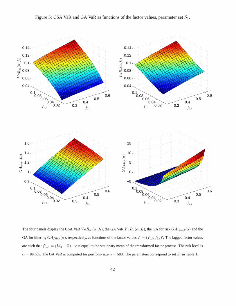
Figure 5: CSA VaR and GA VaR as functions of the factor values, parameter set S1.
0.30.4
0.50.6
0.020.04
0.060.08
0.1
0.04
0.06
0.08
0.1
0.12
0.14
f2,tf1,t
VaR
∞(α
,ft)
0.30.4
0.50.6
0.020.04
0.060.08
0.1
0.04
0.06
0.08
0.1
0.12
0.14
f2,tf1,t
VaR
n(α
,ft)
0.30.4
0.50.6
0.020.04
0.060.08
0.1
0.8
1
1.2
1.4
1.6
f2,tf1,t
GA
ris
k,t(α
)
0.30.4
0.50.6
0.020.04
0.060.08
0.1
−5
0
5
10
15
f2,tf1,t
GA
fil
t,t(α
)
The four panels display the CSA VaR V aR∞(α; ft), the GA VaR V aRn(α; ft), the GA for risk GArisk,t(α) and the
GA for filtering GAfilt,t(α), respectively, as functions of the factor values ft = (f1,t, f2,t)′. The lagged factor values
are such that f∗t−1 = (Id2 − Φ)−1c is equal to the stationary mean of the transformed factor process. The risk level is
α = 99.5%. The GA VaR is computed for portfolio size n = 500. The parameters correspond to set S1 in Table 1.
42
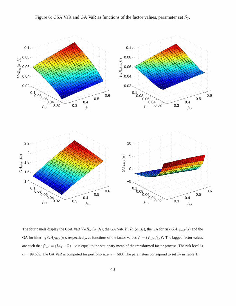
Figure 6: CSA VaR and GA VaR as functions of the factor values, parameter set S2.
0.30.4
0.50.6
0.020.04
0.060.08
0.1
0.02
0.04
0.06
0.08
0.1
f2,tf1,t
VaR
∞(α
,ft)
0.30.4
0.50.6
0.020.04
0.060.08
0.1
0.02
0.04
0.06
0.08
0.1
f2,tf1,t
VaR
n(α
,ft)
0.30.4
0.50.6
0.020.04
0.060.08
0.1
1.4
1.6
1.8
2
2.2
f2,tf1,t
GA
ris
k,t(α
)
0.30.4
0.50.6
0.020.04
0.060.08
0.1
−5
0
5
10
f2,tf1,t
GA
fil
t,t(α
)
The four panels display the CSA VaR V aR∞(α; ft), the GA VaR V aRn(α; ft), the GA for risk GArisk,t(α) and the
GA for filtering GAfilt,t(α), respectively, as functions of the factor values ft = (f1,t, f2,t)′. The lagged factor values
are such that f∗t−1 = (Id2 − Φ)−1c is equal to the stationary mean of the transformed factor process. The risk level is
α = 99.5%. The GA VaR is computed for portfolio size n = 500. The parameters correspond to set S2 in Table 1.
43
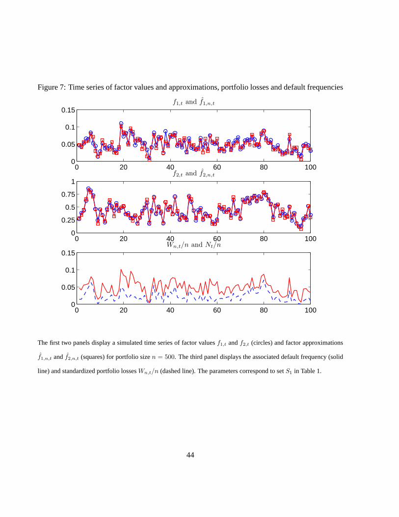
Figure 7: Time series of factor values and approximations, portfolio losses and default frequencies
0 20 40 60 80 1000
0.05
0.1
0.15f1,t and f1,n,t
0 20 40 60 80 1000
0.25
0.5
0.75
1f2,t and f2,n,t
0 20 40 60 80 1000
0.05
0.1
0.15Wn,t/n and Nt/n
The first two panels display a simulated time series of factor values f1,t and f2,t (circles) and factor approximations
f1,n,t and f2,n,t (squares) for portfolio size n = 500. The third panel displays the associated default frequency (solid
line) and standardized portfolio losses Wn,t/n (dashed line). The parameters correspond to set S1 in Table 1.
44

Figure 8: Time series of CSA VaR, GA VaR, GA risk and filtering components.
0 10 20 30 40 50 60 70 80 90 1000
0.05
0.1
0.15V aR∞(α, fn,t) and V aRn(α, fn,t)
0 10 20 30 40 50 60 70 80 90 100−0.02
0
0.02
0.04
0.06
0.08GArisk,t(α) and GAfilt,t(α)
The upper panel displays the CSA VaR V aR∞(α; fn,t) (dashed line) and the GA VaR V aRn(α; fn,t) (solid line). The
lower panel display the risk (dashed line) and filtering (solid line) components of the GA. The risk level is α = 99.5%
and the portfolio size is n = 500. The parameters correspond to set S1 in Table 1.
45
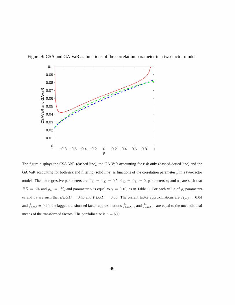
Figure 9: CSA and GA VaR as functions of the correlation parameter in a two-factor model.
−1 −0.8 −0.6 −0.4 −0.2 0 0.2 0.4 0.6 0.8 10
0.01
0.02
0.03
0.04
0.05
0.06
0.07
0.08
0.09
0.1
ρ
CS
AV
aR a
nd G
AV
aR
The figure displays the CSA VaR (dashed line), the GA VaR accounting for risk only (dashed-dotted line) and the
GA VaR accounting for both risk and filtering (solid line) as functions of the correlation parameter ρ in a two-factor
model. The autoregressive parameters are Φ11 = Φ22 = 0.5, Φ12 = Φ21 = 0, parameters c1 and σ1 are such that
PD = 5% and ρD = 1%, and parameter γ is equal to γ = 0.10, as in Table 1. For each value of ρ, parameters
c2 and σ2 are such that ELGD = 0.45 and V LGD = 0.05. The current factor approximations are f1,n,t = 0.04
and f2,n,t = 0.40, the lagged transformed factor approximations f∗1,n,t−1 and f∗
2,n,t−1 are equal to the unconditional
means of the transformed factors. The portfolio size is n = 500.
46
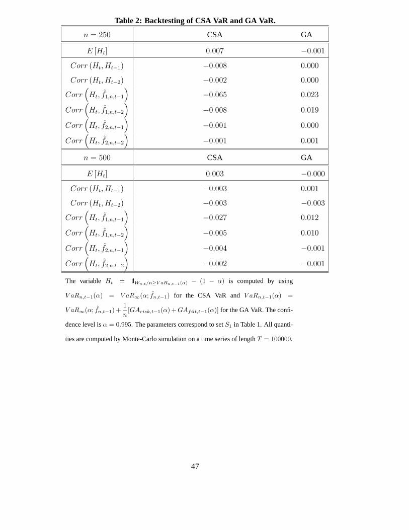
Table 2: Backtesting of CSA VaR and GA VaR.
n = 250 CSA GA
E [Ht] 0.007 −0.001
Corr (Ht, Ht−1) −0.008 0.000
Corr (Ht, Ht−2) −0.002 0.000
Corr(Ht, f1,n,t−1
)−0.065 0.023
Corr(Ht, f1,n,t−2
)−0.008 0.019
Corr(Ht, f2,n,t−1
)−0.001 0.000
Corr(Ht, f2,n,t−2
)−0.001 0.001
n = 500 CSA GA
E [Ht] 0.003 −0.000
Corr (Ht, Ht−1) −0.003 0.001
Corr (Ht, Ht−2) −0.003 −0.003
Corr(Ht, f1,n,t−1
)−0.027 0.012
Corr(Ht, f1,n,t−2
)−0.005 0.010
Corr(Ht, f2,n,t−1
)−0.004 −0.001
Corr(Ht, f2,n,t−2
)−0.002 −0.001
The variable Ht = 1lWn,t/n≥V aRn,t−1(α) − (1 − α) is computed by using
V aRn,t−1(α) = V aR∞(α; fn,t−1) for the CSA VaR and V aRn,t−1(α) =
V aR∞(α; fn,t−1) +1n
[GArisk,t−1(α) + GAfilt,t−1(α)] for the GA VaR. The confi-
dence level is α = 0.995. The parameters correspond to set S1 in Table 1. All quanti-
ties are computed by Monte-Carlo simulation on a time series of length T = 100000.
47
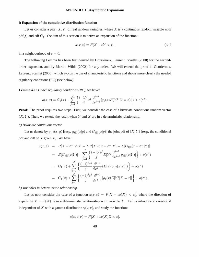
APPENDIX 1: Asymptotic Expansions
i) Expansion of the cumulative distribution function
Let us consider a pair (X, Y ) of real random variables, where X is a continuous random variable with
pdf f1 and cdf G1. The aim of this section is to derive an expansion of the function:
a(x, ε) = P [X + εY < x], (a.1)
in a neighbourhood of ε = 0.
The following Lemma has been first derived by Gourieroux, Laurent, Scaillet (2000) for the second-
order expansion, and by Martin, Wilde (2002) for any order. We will extend the proof in Gourieroux,
Laurent, Scaillet (2000), which avoids the use of characteristic functions and shows more clearly the needed
regularity conditions (RC) (see below).
Lemma a.1: Under regularity conditions (RC), we have:
a(x, ε) = G1(x) +J∑
j=1
{(−1)j
j!εj dj−1
dxj−1[g1(x)E(Y j |X = x)]
}+ o(εJ).
Proof: The proof requires two steps. First, we consider the case of a bivariate continuous random vector
(X, Y ). Then, we extend the result when Y and X are in a deterministic relationship.
a) Bivariate continuous vector
Let us denote by g1,2(x, y) [resp. g1|2(x|y) and G1|2(x|y)] the joint pdf of (X, Y ) (resp. the conditional
pdf and cdf of X given Y ). We have:
a(x, ε) = P [X + εY < x] = EP [X < x − εY |Y ] = E[G1|2(x − εY |Y )]
= E[G1|2(x|Y )] +J∑
j=1
{(−1)jεj
j!E[Y j dj−1
dxj−1g1|2(x|Y )]
}+ o(εJ)
= G1(x) +J∑
j=1
{(−1)jεj
j!dj−1
dxj−1(E[Y jg1|2(x|Y )])
}+ o(εJ)
= G1(x) +J∑
j=1
{(−1)jεj
j!dj−1
dxj−1[g1(x)E[Y j |X = x]]
}+ o(εJ).
b) Variables in deterministic relationship
Let us now consider the case of a function a(x, ε) = P [X + εc(X) < x], where the direction of
expansion Y = c(X) is in a deterministic relationship with variable X . Let us introduce a variable Z
independent of X with a gamma distribution γ(ν, ν), and study the function:
a(x, ε; ν) = P [X + εc(X)Z < x].
48
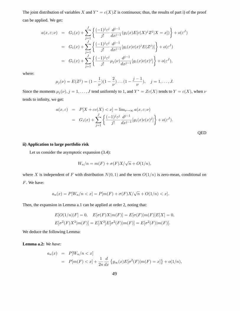
The joint distribution of variables X and Y ∗ = c(X)Z is continuous; thus, the results of part i) of the proof
can be applied. We get:
a(x, ε; ν) = G1(x) +J∑
j=1
{(−1)jεj
j!dj−1
dxj−1(g1(x)E[c(X)jZj |X = x])
}+ o(εJ)
= G1(x) +J∑
j=1
{(−1)jεj
j!dj−1
dxj−1[g1(x)c(x)jE(Zj)]
}+ o(εJ)
= G1(x) +J∑
j=1
{(−1)jεj
j!μj(ν)
dj−1
dxj−1[g1(x)c(x)j ]
}+ o(εJ),
where:
μj(ν) = E(Zj) = (1 − 1ν
)(1 − 2ν
) . . . (1 − j − 1ν
), j = 1, . . . , J.
Since the moments μj(ν), j = 1, . . . , J tend uniformly to 1, and Y ∗ = Zc(X) tends to Y = c(X), when ν
tends to infinity, we get:
a(x, ε) = P [X + εc(X) < x] = limν→∞ a(x, ε; ν)
= G1(x) +J∑
j=1
{(−1)jεj
j!dj−1
dxj−1[g1(x)c(x)j ]
}+ o(εJ).
QED
ii) Application to large portfolio risk
Let us consider the asymptotic expansion (3.4):
Wn/n = m(F ) + σ(F )X/√
n + O(1/n),
where X is independent of F with distribution N(0, 1) and the term O(1/n) is zero-mean, conditional on
F . We have:
an(x) = P [Wn/n < x] = P [m(F ) + σ(F )X/√
n + O(1/n) < x].
Then, the expansion in Lemma a.1 can be applied at order 2, noting that:
E[O(1/n)|F ] = 0, E[σ(F )X|m(F )] = E[σ(F )|m(F )]E[X] = 0,
E[σ2(F )X2|m(F )] = E[X2]E[σ2(F )|m(F )] = E[σ2(F )|m(F )].
We deduce the following Lemma:
Lemma a.2: We have:
an(x) = P [Wn/n < x]
= P [m(F ) < x] +12n
d
dx
{g∞(x)E[σ2(F )|m(F ) = x]
}+ o(1/n),
49

where g∞ is the pdf of m(F ).
Note that this approximation at order 1/n is exact and not itself approximated by the cdf based on a bivariate
distribution as in Vasicek (2002).
iii) Expansion of the VaR
The expansion of the VaR per individual is deduced from the Bahadur’s expansion [see Bahadur (1966),
or Gagliardini, Gourieroux (2010b), Section 6.2].
Lemma a.3 (Bahadur’s expansion): Let us consider a sequence of cdf’s Fn tending to a limiting cdf F∞
at uniform rate 1/n:
Fn(x) = F∞(x) + O(1/n).
Let us denote by Qn and Q∞ the associated quantile functions and assume that the limiting distribution is
continuous with density f∞. Then:
Qn(α) − Q∞(α) = −Fn[Q∞(α)] − F∞[Q∞(α)]f∞[Q∞(α)]
+ o(1/n).
Lemma a.3 can be applied to the standardized portfolio risk. The limiting distribution is the distribution
of m(F ) with pdf g∞ and quantile function V aR∞. By using the expansion of Lemma a.2, we get:
V aRn(α) = V aR∞(α) − 12n
1g∞[V aR∞(α)]
[d
dx
{g∞(x)E[σ2(F )|m(F ) = x]
}]x=V aR∞(α)
+o(1/n)
= V aR∞(α) − 12n
{d log g∞
dx[V aR∞(α)]E[σ2(F )|m(F ) = V aR∞(α)]
+[
d
dxE[σ2(F )|m(F ) = x]
]x=V aR∞(α)
}+ o(1/n).
This is the result in Proposition 1.
50
APPENDIX 2: Aggregation of risk measures
The aggregation of risk measures, in particular of VaR, is a difficult task. In this Appendix we consider
this question in a large portfolio perspective for a single factor model. Let us index by k = 1, · · · , K
the different subpopulations, with respective weights πk, k = 1, · · · , K. Within subpopulation k, the
conditional mean and variance given factor F are denoted mk(F ) and σ2k(F ), respectively. At population
level, the conditional mean is:
m(F ) =K∑
k=1
πkmk(F ), (a.2)
by the iterated expectation theorem, and the conditional variance is given by:
σ2(F ) =K∑
k=1
πkσ2k(F ) +
K∑k=1
πk [mk(F ) − m(F )]2 , (a.3)
by the variance decomposition equation. We denote by Q∞, G∞ and g∞ the quantile, cdf and pdf of the
distribution of factor F , respectively.
i) Aggregation of CSA risk measures
We assume:
A.3: The conditional means mk(F ) are increasing functions of F , for any k = 1, · · · , K.
Under Assumption A.3, the systematic risk components mk(F ), k = 1, · · · , K are co-monotonic [see
McNeil, Frey, Embrechts (2005), Proposition 6.15]. Therefore, we have:
P[m(F ) < V aR∞(α)
]= α ⇔ P
[F < m−1
(V aR∞(α)
)]= α,
and we deduce that the VaR at population level is:
V aR∞(α) = m[Q∞(α)] =K∑
k=1
πkmk[Q∞(α)] =K∑
k=1
πkV aRk,∞(α), (a.4)
by definition of the disaggregated VaR. We have the perfect aggregation formula for the CSA risk measure,
that is, the aggregate VaR is obtained by summing the disaggregated VaR with the subpopulation weights.
ii) Aggregation of Granularity Adjustments
We have the following result:
51

Lemma a.4: The aggregate granularity adjustment is given by:
GA(α) = −12
⎧⎪⎪⎪⎪⎪⎨⎪⎪⎪⎪⎪⎩
⎛⎜⎜⎜⎜⎜⎝
d log g∞dF
[Q∞(α)]1
K∑k=1
πkdmk
dF[Q∞(α)]
−
K∑k=1
πkd2mk
dF 2[Q∞(α)]
(K∑
k=1
πkdmk
dF[Q∞(α)]
)2
⎞⎟⎟⎟⎟⎟⎠
·(
K∑k=1
πkσ2k[Q∞(α)] +
K∑k=1
πk (mk[Q∞(α)] − m[Q∞(α)])2)
+
K∑k=1
πkdσ2
k
dF[Q∞(α)] +
d
dF
{K∑
k=1
πk (mk(F ) − m(F ))2}
F=Q∞(α)
K∑k=1
πkdmk
dF[Q∞(α)]
⎫⎪⎪⎪⎪⎪⎪⎬⎪⎪⎪⎪⎪⎪⎭
.
Proof: Let us compute the different terms in the GA formula in Proposition 1 by using the population
conditional mean and variance components given in (a.2) and (a.3).
i) The conditional expectation of σ2(F ) given m(F ) is:
E[σ2(F )|m(F ) = z] = E[σ2(F )|F = m−1(z)] = σ2[m−1(z)].
Then, from (a.4) we get:
E[σ2(F )|m(F ) = V aR∞(α)]
= σ2[Q∞(α)] =K∑
k=1
πkσ2k[Q∞(α)] +
K∑k=1
πk (mk[Q∞(α)] − m[Q∞(α)])2 , (a.5)
and similarly:
E[σ2k(F )|mk(F ) = V aRk,∞(α)] = σ2
k[Q∞(α)]. (a.6)
ii) The derivative of the conditional expectation of σ2(F ) given m(F ) = z w.r.t. z is given by:
∂
∂zE[σ2(F )|m(F ) = z] =
∂
∂zσ2[m−1(z)] =
dσ2
dF[m−1(z)]
1dm
dF[m−1(z)]
.
Thus:
∂
∂zE[σ2(F )|m(F ) = z]
∣∣∣∣z=V aR∞(α)
=
dσ2
dF[Q∞(α)]
dm
dF[Q∞(α)]
. (a.7)
Similarly:
∂
∂zE[σ2
k(F )|mk(F ) = z]∣∣∣∣z=V aRk,∞(α)
=
dσ2k
dF[Q∞(α)]
dmk
dF[Q∞(α)]
. (a.8)
52

iii) Let us now derive the distribution m(F ). We have:
P [m(F ) ≤ z] = P [F ≤ m−1(z)] = G∞[m−1(z)].
Thus, the pdf of m(F ) is given by:
g∞(z) = g∞[m−1(z)]1
dm
dF[m−1(z)]
.
The derivative of the log-density is:
d log g∞(z)dz
=d
dz
[log g∞[m−1(z)] − log
dm
dF[m−1(z)]
]
=
⎛⎜⎜⎜⎝d log g∞(F )
dF
1dm
dF(F )
−d2m
dF 2(F )[
dm
dF(F )]2⎞⎟⎟⎟⎠
F=m−1(z)
.
Thus, we get:
d log g∞dz
[V aR∞(α)] =d log g∞
dF[Q∞(α)]
1dm
dF[Q∞(α)]
−d2m
dF 2[Q∞(α)](
dm
dF[Q∞(α)]
)2 . (a.9)
Similarly:
d log gk,∞dz
[V aRk,∞(α)] =d log g∞
dF[Q∞(α)]
1dmk
dF[Q∞(α)]
−d2mk
dF 2[Q∞(α)](
dmk
dF[Q∞(α)]
)2 . (a.10)
From (a.5), (a.7) and (a.9), and Proposition 1, the GA in Lemma a.4 follows.
QED
In general, the aggregate GA cannot be written as a function of the subpopulations weights, disaggregate
CSA VaR and disaggregate GA, given by [use equations (a.6), (a.8) and (a.10), and Proposition 1]:
GAk(α) = −12
⎧⎪⎪⎨⎪⎪⎩
⎛⎜⎜⎝d log g∞
dF[Q∞(α)] −
d2mk
dF 2[Q∞(α)]
dmk
dF[Q∞(α)]
⎞⎟⎟⎠ σ2
k[Q∞(α)]dmk
dF[Q∞(α)]
+
dσ2k
dF[Q∞(α)]
dmk
dF[Q∞(α)]
⎫⎪⎪⎬⎪⎪⎭ .
(a.11)
This shows that the difficulty in aggregating the risk measures is due mainly to the idiosyncratic risk.
53

Perfect aggregation applies for the GA if the subpopulations are homogeneous w.r.t. the systematic risk
component, that is, if functions mk(.) are independent of k.
Corollary 1: If mk(F ) is independent of k = 1, · · · , K, we have:
GA(α) =K∑
k=1
πkGAk(α).
Proof: This is a direct consequence of the GA formula given in Lemma a.4.
When functions mk(.) differ across the subpopulations, Lemma a.4 implies that the aggregate GA is
equal to a weighted average of the disaggregate GA, with modified weights that differ from the population
weights, plus some correction terms that account for heterogeneity. As an example, let us suppose that the
systematic risk components are linear with different factor loadings across the subpopulations:
mk(F ) = βkF, k = 1, · · · , K,
with the normalizationK∑
k=1
πkβk = 1. Then, we have m(F ) = F and from Lemma a.4 we get:
GA(α) =K∑
k=1
βkπkGAk(α) − 12γ2
(d log g∞
dF[Q∞(α)]Q∞(α)2 + 2Q∞(α)
), (a.12)
where γ2 =K∑
k=1
πk(βk − 1)2 and:
GAk(α) = − 12βk
(d log g∞
dF[Q∞(α)]σ2
k[Q∞(α)] +dσ2
k
dF[Q∞(α)]
).
The first term in (a.12) is a weighted average of disaggregated GA with weights proportional to the products
of betas by population frequencies. The second term is an adjustment for beta heterogeneity. It involves the
variance of betas γ2 as heterogeneity measure, multiplied by quantity
−12
(d log g∞
dF[Q∞(α)]Q∞(α)2 + 2Q∞(α)
), which corresponds to the GA computed with m(F ) = F
and σ2(F ) = F 2. When the systematic factor F is Gaussian and the conditional variance functions
σ2k(F ) = σ2 are constant, independent of k, equation (a.12) corresponds to the GA for the linear static
RFM with discrete beta heterogeneity (see Example 4.3).
54

APPENDIX 3: GA when m(F ) is monotone increasing
From Proposition 1 we have:
GA(α) = −12
(1
g∞(z)d
dz
{g∞(z)E
[σ2(F )|m(F ) = z
]})z=V aR∞(α)
= −12
(1
g∞(z)d
dz
{g∞(z)σ2[m−1(z)]
})z=V aR∞(α)
= −12
⎛⎜⎝
dm
dF[m−1(z)]
g∞[m−1(z)]d
dz
⎧⎪⎨⎪⎩
g∞[m−1(z)]σ2[m−1(z)]dm
dF[m−1(z)]
⎫⎪⎬⎪⎭⎞⎟⎠
z=V aR∞(α)
= −12
⎛⎜⎝ 1
g∞[m−1(z)]d
dm−1(z)
⎧⎪⎨⎪⎩
g∞[m−1(z)]σ2[m−1(z)]dm
dF[m−1(z)]
⎫⎪⎬⎪⎭⎞⎟⎠
z=V aR∞(α)
= −12
⎛⎜⎝ 1
g∞(f)d
df
⎧⎪⎨⎪⎩
g∞(f)σ2(f)dm
dF(f)
⎫⎪⎬⎪⎭⎞⎟⎠
f=m−1[V aR∞(α)]
.
APPENDIX 4: Granularity adjustment in the Merton-Vasicek model
In this Appendix we prove equation (4.9) for the GA in the Merton Vasicek model. From (4.4)-(4.7) we
get:
GA(α) = −12
⎧⎪⎪⎪⎨⎪⎪⎪⎩
Φ−1(PD)√1 − ρ
− 1 − 2ρ√ρ(1 − ρ)
Φ−1(α)
φ
(Φ−1(PD) +
√ρΦ−1(α)√
1 − ρ
) V aR∞(α)[1 − V aR∞(α)] +1 − 2V aR∞(α)}
.
Now, we have:
Φ−1(PD)√1 − ρ
− 1 − 2ρ√ρ(1 − ρ)
Φ−1(α) =Φ−1(PD) +
√ρΦ−1(α)√
1 − ρ−√
1 − ρ
ρΦ−1(α)
= Φ−1 [V aR∞(α)] −√
1 − ρ
ρΦ−1(α).
Then, equation (4.9) follows.
55

APPENDIX 5: Stochastic probability of default and expected loss given default
In this Appendix we give a detailed derivation of the granularity adjustment in the model with stochastic
probability of default and expected loss given default presented in Section 6.
i) ELGD and VLGD
The unconditional expected loss given default is:
ELGD = E[LGDi,t|Zi,t = 1] = E[E[LGDi,t|Ft, Zi,t = 1]|Zi,t = 1] = E[F2,t|Zi,t = 1]
=E[F2,t1lZi,t=1]
E[1lZi,t=1]=
E[F2,tE[Zi,t|Ft]]E[Zi,t]
=E[F2,tF1,t]
E[F1,t]= E∗[F2,t],
where E∗[·] denotes expectation w.r.t. the probability distribution defined by the change of measure F1,t/E[F1,t].
The unconditional variance of the loss given default is:
V LGD = V [LGDi,t|Zi,t = 1] = E[LGD2i,t|Zi,t = 1] − ELGD2
= E[E[LGD2i,t|Ft, Zi,t = 1]|Zi,t = 1] − ELGD2
= E[V [LGDi,t|Ft]|Zi,t = 1] + E[E[LGDi,t|Ft]2|Zi,t = 1] − ELGD2
= γE[F2,t(1 − F2,t)|Zi,t = 1] + E[F 22,t|Zi,t = 1] − ELGD2
= (1 − γ)E[F 22,t|Zi,t = 1] + ELGD(γ − ELGD)
= (1 − γ)E[F 2
2,tF1,t]E[F1,t]
+ ELGD(γ − ELGD)
= γELGD(1 − ELGD) + (1 − γ)
(E[F 2
2,tF1,t]E[F1,t]
− ELGD2
).
Thus we get:
V LGD = γELGD(1 − ELGD) + (1 − γ)V ∗[F2,t].
ii) Cross-sectional factor approximation
Let us consider date t and assume that we observe the individual losses yi,t, i = 1, · · · , n, of the zero-
coupon corporate bonds maturing at date t. Equivalently, we observe the default indicator Zi,t = 1lyi,t>0
for all individual companies, and the Loss Given Default LGDi,t = yi,t, if Zi,t = 1. Thus, the model is
equivalent to a tobit model and the cross-sectional likelihood conditional on the factor value is:
n∏i=1
h(yi,t|ft) =
[n∏
i=1
fZi,t
1,t (1 − f1,t)1−Zi,t
] ∏i:Zi,t=1
Γ(at + bt)Γ(at)Γ(bt)
LGDat−1i,t (1 − LGDi,t)bt−1
= fNt1,t (1 − f1,t)n−Nt
(Γ[(1 − γ)/γ]Γ(at)Γ(bt)
)Nt
⎡⎣ ∏
i:yi,t>0
yi,t
⎤⎦
at−1 ⎡⎣ ∏
i:yi,t>0
(1 − yi,t)
⎤⎦
bt−1
,
56
where Nt =n∑
i=1
1lyi,t>0 is the number of defaults at date t, and at =(
1 − γ
γ
)f2,t and bt =
(1 − γ
γ
)(1−
f2,t). We get the cross-sectional log-likelihood:
n∑i=1
log h(yi,t|ft) = Nt log f1,t + (n − Nt) log(1 − f1,t) + Nt log Γ[1 − γ
γ
]
−Nt log Γ[(
1 − γ
γ
)f2,t
]− Nt log Γ
[(1 − γ
γ
)(1 − f2,t)
]
+[(
1 − γ
γ
)f2,t − 1
] ∑i:yi,t>0
log yi,t +[(
1 − γ
γ
)(1 − f2,t) − 1
] ∑i:yi,t>0
log(1 − yi,t)
= L1,n,t(f1,t) + L2,n,t(f2,t), say. (a.13)
which is decomposed as the sum of a function of f1,t and a function of f2,t. Therefore, the cross-sectional
approximations of the two factors can be computed separately, and we get (6.1) and (6.2).
iii) Approximate filtering distribution of ft given In,t
From a multiple factor version of Corollary 5.3 in Gagliardini, Gourieroux (2010a), and the log-likelihood
decomposition in (a.13), it follows that the approximate filtering distribution is such that F1,t and F2,t are in-
dependent conditional on information In,t at order 1/n, with Gaussian distributions N
(fl,n,t +
1n
μl,n,t,1n
J−1l,n,t
),
for l = 1, 2, where:
μl,n,t = J−1l,n,t
∂ log g
∂fl,t(fn,t|fn,t−1) +
12J−2
l,n,tKl,n,t,
Jl,n,t = − 1n
n∑i=1
∂2 log h
∂f2l,t
(yi,t|fn,t) = − 1n
∂2Ll,n,t
∂f2l,t
(fl,n,t),
Kl,n,t =1n
n∑i=1
∂3 log h
∂f3l,t
(yi,t|fn,t) =1n
∂3Ll,n,t
∂f3l,t
(fl,n,t),
and where g denotes the transition pdf of factor Ft. From (a.13), equations (6.4) and (6.5) follow, as well as
K1,n,t = 21 − 2f1,n,t
f21,n,t(1 − f1,n,t)2
. Moreover:
∂ log g
∂fl,t(ft|ft−1) = − 1
a[A−1(fl,t)]
{e′l[Ω−1(f∗
t − c − Φf∗t−1)]+
d log a
dy[A−1(fl,t)]
}
= − 1fl,t(1 − fl,t)
{e′l[Ω−1(f∗
t − c − Φf∗t−1)]+ 1 − 2fl,t
},
for l = 1, 2, where A(y) = [1 + exp(−y)]−1 and a(y) = dA(y)/dy. Then equations (6.3) follow.
iv) A useful lemma
The derivation of the CSA VaR and the GA below uses the next lemma.
57
Lemma a.5: Let X and Y be two random variables on [0, 1]. Denote by f(x, y), f2(y), F2(y) and F1|2(x|y)
the joint pdf of (X, Y ), the pdf of Y , the cdf of Y and the conditional cdf of X given Y = y, respectively.
Let Z = XY . Then:
(i) P [Z ≤ z] =∫ 1
zF1|2(z/y|y)f2(y)dy + F2(z), for any z ∈ [0, 1];
(ii) The pdf of Z is g(z) =∫ 1
z
1yf(z/y, y)dy, z ∈ [0, 1];
(iii) E[Y |Z = z] =
∫ 1
zf(z/y, y)dy∫ 1
z
1yf(z/y, y)dy
, for any z ∈ [0, 1].
Proof: (i) We have:
P [Z ≤ z] = EP [Z ≤ z|Y ] = EP [X ≤ z/Y |Y ].
Now, P [X ≤ z/Y |Y ] = 1lz≤Y F1|2(z/Y |Y ) + 1lz>Y . Thus, we get:
P [Z ≤ z] =∫ 1
zF1|2(z/y|y)f2(y)dy + F2(z).
(ii) By differentiating the cdf found in (i) we get:
g(z) =d
dz
(∫ 1
zF1|2(z/y|y)f2(y)dy + F2(z)
)
=∫ 1
z
1yf(z/y|y)f2(y)dy − [F1|2(z/y|y)f2(y)
]y=z
+ f2(z) =∫ 1
z
1yf(z/y, y)dy.
(iii) Let us consider the change of variables from (x, y) to (z, y), where z = xy. The Jacobian is
∣∣∣∣det[
∂(z, y)∂(x, y)
]∣∣∣∣ =y. Thus, the joint density of Z and Y is g(z, y) =
1yf(z/y, y), for 0 ≤ z ≤ y ≤ 1. We get:
E[Y |Z = z] =
∫ 1
zyg(z, y)dy∫ 1
zg(z, y)dy
=
∫ 1
zf(z/y, y)dy∫ 1
z
1yf(z/y, y)dy
.
QED
v) CSA risk measure
Let us first compute function a(w, 0; f). We have:
m(Ft+1) = E[LGDi,t+1|Ft+1]E[Zi,t+1|Ft+1] = F1,t+1F2,t+1. (a.14)
58

Then, from (5.6):
a(w, 0; ft) = P [F1,t+1F2,t+1 ≤ w|Ft = ft].
Let us apply Lemma a.5 (i) with X = F2,t+1 and Y = F1,t+1, conditionally on Ft = ft. The distribution of
F ∗2,t+1 conditional on F ∗
1,t+1 and Ft = ft is:
N
(c2,t +
ρσ2
σ1(F ∗
1,t+1 − c1,t), σ22(1 − ρ2)
),
where c1,t = c1 + Φ11A−1(f1,t) + Φ12A
−1(f2,t) and c2,t = c2 + Φ21A−1(f1,t) + Φ22A
−1(f2,t). Thus, the
conditional cdf of F2,t+1 given F1,t+1 = y and Ft = ft is:
P [F2,t+1 ≤ x|F1,t+1 = y, Ft = ft] = Φ
⎡⎢⎣A−1(x) − c2,t − ρσ2
σ1(A−1(y) − c1,t)
σ2
√1 − ρ2
⎤⎥⎦ ,
for x, y ∈ (0, 1). The cdf and the pdf of F1,t+1 conditional on Ft = ft are:
F (y|ft) = Φ(
A−1(y) − c1,t
σ1
), f(y|ft) =
1σ1
ϕ
(A−1(y) − c1,t
σ1
)1
a[A−1(y)],
respectively, where a(y) = dA(y)/dy. Thus, from Lemma a.5 we get:
a(w, 0; ft) = Φ(
A−1(w) − c1,t
σ1
)+∫ 1
wΦ
⎡⎢⎣A−1(w/y) − c2,t − ρσ2
σ1(A−1(y) − c1,t)
σ2
√1 − ρ2
⎤⎥⎦
· 1σ1
ϕ
(A−1(y) − c1,t
σ1
)1
a[A−1(y)]dy.
By using that a[A−1(y)] = y(1 − y) and A−1(y) = log[y/(1 − y)], Proposition 5 i) follows.
vi) Granularity adjustment
Let us first compute the conditional density g∞(.; ft) of m(Ft+1) given Ft = ft. We use equation (a.14)
and apply Lemma a.5 (ii) with X = F1,t+1 and Y = F2,t+1 conditionally on Ft = ft. The joint density of
(X, Y ) conditionally on Ft = ft is:
f(x, y) =1
σ1σ2ϕ
(A−1(x) − c1,t
σ1,A−1(y) − c2,t
σ2; ρ)
1a[A−1(x)]a[A−1(y)]
,
where ϕ(., .; ρ) denotes the pdf of a bivariate standard Gaussian distribution with correlation parameter ρ.
We get:
g∞(w; ft) =∫ 1
w
1y
1σ1σ2
ϕ
(A−1 (w/y) − c1,t
σ1,A−1(y) − c2,t
σ2; ρ)
1a[A−1 (w/y)]a[A−1(y)]
dy.
59

Let us now compute E[σ2(Ft+1)|m(Ft+1) = w, Ft = ft]. We have:
σ2(Ft+1) = E[LGD2i,t+1|Ft+1]E[Zi,t+1|Ft+1] − E[LGDi,t+1|Ft+1]2E[Zi,t+1|Ft+1]2
= γF2,t+1(1 − F2,t+1)F1,t+1 + F1,t+1(1 − F1,t+1)F 22,t+1,
By replacing F1,t+1F2,t+1 with m(Ft+1) in the above equation, function σ2(Ft+1) can be rewritten as:
σ2(Ft+1) = γ(F1,t+1F2,t+1)(1 − F2,t+1) + (F1,t+1F2,t+1)(F2,t+1 − F1,t+1F2,t+1)
= m(Ft+1)[γ − m(Ft+1)] + (1 − γ)m(Ft+1)F2,t+1.
Thus:
E[σ2(Ft+1)|m(Ft+1) = w, Ft = ft] = w(γ − w)
+(1 − γ)wE[F2,t+1|F1,t+1F2,t+1 = w, Ft = ft]. (a.15)
From Lemma a.5 (iii) with X = F1,t+1 and Y = F2,t+1, conditionally on Ft = ft, we get:
E[F2,t+1|m(Ft+1) = w, Ft = ft] =b(w, 1; ft)g∞(w; ft)
,
where:
b(w, 1; ft) =∫ 1
w
1σ1σ2
ϕ
(A−1 (w/y) − c1,t
σ1,A−1(y) − c2,t
σ2; ρ)
1a[A−1 (w/y)]a[A−1(y)]
dy.
Then, from equation (a.15) we get:
E[σ2(Ft+1)|m(Ft+1) = w, Ft = ft] = w(γ − w) + (1 − γ)wb(w, 1; ft)g∞(w; ft)
.
By using a[A−1 (w/y)]a[A−1(y)] = w(y − w)(1 − y)/y, Proposition 5 ii) follows.
60
Related Documents