GRADUATE ALGEBRA: NUMBERS, EQUATIONS, SYMMETRIES

GRADUATE ALGEBRA: NUMBERS, EQUATIONS, SYMMETRIES

JENIA TEVELEV

CONTENTS

§1. Algebraic Field Extensions§1.1. Field extensions§1.2. Multiplicativity of degree§1.3. Algebraic extensions§1.4. Adjoining roots§1.5. Splitting fields§1.6. Algebraic closure§1.7. Finite fields§1.8. Exercises§2. Galois Theory§2.1. Separable extensions§2.2. Normal extensions§2.3. Main Theorem of Galois Theory§2.4. Fields of invariants§2.5. Exercises§3. First Applications of Galois Theory§3.1. Translations from group theory to Galois theory§3.2. Fundamental Theorem of Algebra§3.3. Quadratic extensions§3.4. Cubic extensions§3.5. Galois group of a finite field§3.6. Exercises§4. Adjoining Radicals§4.1. Adjoining roots of unity§4.2. Cyclotomic fields§4.3. Cyclic extensions§4.4. Artin’s Lemma§4.5. Norm and Trace§4.6. Lagrange resolvents§4.7. Solvable extensions: Galois Theorem.§4.8. Exercises§5. Quadratic Extensions of Q§5.1. Quadratic case of the Kronecker–Weber theorem§5.2. Integral extensions§5.3. Quadratic reciprocity§5.4. Some Examples of the Integral Closure§5.5. Exercises§6. Sample Midterm on Galois Theory

§7. Transcendental numbers and extensions§7.1. Transcendental numbers. Liouville’s Theorem§7.2. Bonus section: proof of Hermite’s Theorem§7.3. Transcendence degree§7.4. Noether’s Normalization Lemma§8. Basic Algebraic Geometry – I§8.1. Weak Nullstellensatz§8.2. Algebraic sets. Strong Nullstellensatz§8.3. Zariski topology on An

§8.4. Irreducible algebraic sets§8.5. Irreducible components§8.6. Affine algebraic sets. Regular functions.§8.7. Morphisms of affine algebraic sets§8.8. Dominant morphisms§9. Localization and local rings§9.1. Examples from number theory and geometry§9.2. Localization of rings§9.3. Extension and contraction of ideals in R and S�1R§9.4. Nilradical§9.5. Going-up Theorem§9.6. Finite morphisms§9.7. Localization of modules§9.8. Localization is exact§9.9. Nakayama’s Lemma§10. Bonus section: a bit more Algebraic Geometry§10.1. Rational functions§10.2. Dimension§10.3. Discrete Valuation Rings§11. Sample midterm§12. Representations of finite groups§12.1. Definition and Examples§12.2. G-modules§12.3. Mashke’s Theorem§12.4. Schur’s Lemma§12.5. One-dimensional representations§12.6. Exercises§13. Irreducible representations of finite groups§13.1. Characters§13.2. Basic operations on representations and their characters§13.3. Schur’s orthogonality relations§13.4. Decomposition of the regular representation§13.5. The number of irreducible representations§13.6. Character table of the dihedral group§13.7. Dimension of an irreducible representation divides |G|§13.8. Burnside’s Theorem§13.9. Exercises

§1. ALGEBRAIC FIELD EXTENSIONS

§1.1. Field extensions. We almost never focus on a single field In alge-bra. Indeed, rings can be understood by describing their ideals or modules.But fields have no proper ideals and modules over a field are vector spaces,the subject of linear algebra. Instead, a typical situation is to have two fields

K ⇢ F.

Then F is called a field extension of K: we extend K by adjoining new ele-ments, for example roots of polynomial equations

R ⇢ C, Q ⇢ Q(p2), . . .

Another notation for a field extension is F/K: F is a field over K.

DEFINITION 1.1.1. A field F over K can be viewed as a vector space over Kby using addition in F to add vectors and using multiplication in F todefine scalar multiplication �x for � 2 K and x 2 F . Its dimension is calledthe degree of F over K:

[F : K] := dimK F.

If [F : K] < 1 then F is called a finite extension of K.

For example, [C : R] = 2. The basis of C over R is given by 1 and i.We also have [Q(

p2) : Q] = 2. The basis is given by 1 and

p2. Indeed,

• 1 andp2 are linearly independent over Q, i.e. a + b

p2 6= 0 if a or b

is not equal to zero. This is becausep2 is irrational,

p2 6= �a/b.

• 1 andp2 generate Q(

p2) as a vector space over Q. Apriori, an ele-

ment of Q(p2) is a fraction a+b

p2

c+dp2

with a, b, c, s 2 Q. However, mul-tiplying the numerator and denominator by c� d

p2 we can rewrite

this fraction as a linear combination of 1 andp2.

DEFINITION 1.1.2. Consider a field extension K ⇢ F . An element ↵ 2 Fis called algebraic over K if ↵ is a root of a non-trivial polynomial withcoefficients in K. An element which is not algebraic is called transcendental.

• i 2 C is a root of x2 + 1 2 Q[x], so i is algebraic over Q.• ⇡ 2 R is transcendental over Q (Lindemann’s Theorem).• x 2 C(x) is transcendental over C. (Why?)

DEFINITION 1.1.3. Consider a field extension K ⇢ F . Let ↵ 2 F be alge-braic. A polynomial f(x) 2 K[x] is called a minimal polynomial of ↵ if f(x)is a monic polynomial of minimal possible degree such that f(↵) = 0.

Let us point out one persistent notational ambiguity. If x is a variablethen K[x] denotes the algebra of polynomials and K(x) denotes the field ofrational functions (i.e. ratios of polynomials) in variable x. But given a fieldextension K ⇢ F and an element ↵ 2 F , K[↵] denotes the minimal subringof F generated by K and by ↵ and K(↵) denotes the minimal subfield of Fgenerated by K and by ↵. These objects are related as follows:

THEOREM 1.1.4. Consider a field extension K ⇢ F . Let ↵ 2 F . Consider aunique surjective homomorphism � : K[x] ! K[↵] that sends x to ↵.

• If ↵ is transcendental then � is an isomorphism, which induces an isomor-phism of fields K(x) ' K(↵). In particular, [K(↵) : K] = 1.

• If ↵ is algebraic then Ker� is generated by the minimal polynomial f(x),which is irreducible and unique. Let n = deg f(x). Then [K(↵) : K] = n.Moreover, K[↵] = K(↵) and 1,↵, . . . ,↵n�1 form a K-basis of K(↵).

Proof. Ker� is an ideal of all polynomials that vanish at ↵. Ker� = 0 if andonly if ↵ is transcendental (by definition). In this case

K[x] ' K[↵] ⇢ F.

Any injective homomorphism of a domain into a field extends to the injec-tive homomorphism of its field of fractions. So in our case � extends to theinjective homomorphism K(x) ! F , and its image is obviously K(↵).

If ↵ is algebraic then, since K[x] is a PID, Ker� is generated by a uniquemonic polynomial f(x), hence a minimal polynomial is unique. Since

K[x]/Ker� ' K[↵]

injects in F , which is a domain, K[x]/Ker� is also a domain, hence f(x)is irreducible and Ker� = (f) is a maximal ideal. So K[x]/Ker� is a field.Therefore, K[↵] is a field. Therefore, K[↵] = K(↵).

Finally, we notice that 1,↵, . . . ,↵n�1 are linearly independent over K(otherwise we can find a smaller degree polynomial vanishing at ↵) andspan K[↵] over K. Indeed, since f(x) = xn + . . . vanishes at ↵, we canrewrite ↵n as a linear combination of smaller powers of ↵. An easy argu-ment by induction shows that we can rewrite any ↵m for m > n as as alinear combination of 1,↵, . . . ,↵n�1. ⇤

An often used corollary:

COROLLARY 1.1.5. If ↵ is algebraic over K then [K(↵) : K] is equal to the degreeof the minimal polynomial of ↵.

The number [K(↵) : K] is also often called the degree of ↵ over K.

EXAMPLE 1.1.6. [Q(p2 +

p3) : Q] = 4. This calculation involves a trick

which will become much more transparent after we discuss Galois theory.The polynomial of degree 4

f(x) =Y

(x±p2±

p3) = x4 � 10x2 + 1

obviously hasp2 +

p3 as a root. To show that it is irreducible, we have

to show that it has no linear and quadratic factors over Q. If it has a linearfactor then

p2±p

3 2 Q, therefore (p2±p

3)2 2 Q, thereforep6 2 Q. Then

we use the standard argument: ifp6 = a/b in lowest terms then a2 = 6b2,

therefore 2|a, therefore 4|a2, therefore 2|b, contradiction. Suppose f(x) hasa quadratic factor over Q. Its coefficients are, up to a sign, a sum and aproduct of two roots of f(x). If the sum belongs to Q then

p2 or

p3 belong

to Q, unless the two roots are opposite, sayp2 +

p3 and �p

2�p3. But if

their product is in Q then againp6 2 Q, a contradiction.

EXAMPLE 1.1.7. [Q( 3p2) : Q] = 3 and the minimal polynomial is x3 � 2

(irreducible by the Eisenstein’s criterion).

§1.2. Multiplicativity of degree.

LEMMA 1.2.1. Consider a tower of field extensions

K ⇢ F ⇢ L.

If [F : K] = n and [L : F ] = m then [L : K] = nm.

Proof. It is easy to prove that if e1, . . . , em is a basis of L over F and f1, . . . , fnis a basis of F over K then {eifj} is a basis of L over K. (Why?) ⇤

This statement has interesting divisibility consequences. For example, ifK/Q is a finite field extension containing

p2, then [K : Q] is even because

[K : Q] = [Q(p2) : Q][K : Q(

p2)] = 2[K : Q(

p2)].

§1.3. Algebraic extensions.

DEFINITION 1.3.1. An extension K ⇢ F is called algebraic if any element ofF is algebraic over K.

THEOREM 1.3.2. (a) Any finite extension is algebraic.(b) Let ↵1, . . . ,↵r ⇢ F be algebraic over K. Then

K(↵1, . . . ,↵r) = K[↵1, . . . ,↵r]

is finite over K. In particular, any element of K(↵1, . . . ,↵r) is algebraic over K.

Proof. If [F : K] < 1 then 1,↵,↵2, . . . are linearly dependent over K forany ↵ 2 F . Therefore, some non-constant polynomial with coefficient in Kvanishes at ↵, i.e. ↵ is algebraic.

Now suppose that ↵1, . . . ,↵r ⇢ F are algebraic over K. Arguing byinduction on r (with the base of induction given by Theorem 1.1.4), let’sassume that K(↵1, . . . ,↵r�1) = K[↵1, . . . ,↵r�1] is finite over K. Since ↵r

is algebraic over K, it is also algebraic over K(↵1, . . . ,↵r�1). Using Theo-rem 1.1.4, we see that

K(↵1, . . . ,↵r�1)[↵r] = K(↵1, . . . ,↵r�1)(↵r) = K(↵1, . . . ,↵r�1,↵r)

is finite-dimensional over K(↵1, . . . ,↵r�1). Then [K(↵1, . . . ,↵r) : K] < 1by Lemma 1.2.1. It follows from part (a) that any element of K(↵1, . . . ,↵r)is algebraic over K. ⇤

One consequence of this theorem is that if ↵ and � are algebraic over Kthen so are ↵ + �, ↵�, and ↵/�. However, it can take some work to writetheir minimal polynomials, as Example 1.1.6 shows.

§1.4. Adjoining roots. In the previous section we studied a fixed extensionK ⇢ F . If ↵ 2 F is algebraic over K then K(↵) is isomorphic to K[x]/(f),where f(x) is a minimal polynomial of ↵. An algebraic extension

K ⇢ K(↵)

generated by one element is called a simple extension. Now we start witha field K and learn how to build its simple extensions and compare them.The main building block was discovered by Kronecker:

LEMMA 1.4.1. If f(x) 2 K[x] is irreducible and monic then K[x]/(f) is a fieldextension of K generated by ↵ := x+ (f). The minimal polynomial of ↵ is f(x).

Proof. Since f is irreducible and K[x] is a PID, K[x]/(f) is a field. It isobviously generated by ↵. Since f(↵) ⌘ 0 mod (f) in the quotient ring,↵ is a root of f(x). Since f(x) is irreducible over K, f(x) is the minimalpolynomial of ↵. ⇤DEFINITION 1.4.2. Let F and F 0 be field extensions of K. Then F and F 0are called isomorphic over K if there exists an isomorphism � : F ! F 0 suchthat �|K = Id. More generally, we can talk about homomorphisms over K.

LEMMA 1.4.3. Let K(↵) and K(�) be algebraic extensions of K. TFAE:• ↵ and � have the same minimal polynomial.• There exists and isomorphism of K(↵) to K(�) over K that sends ↵ to �.

Proof. If ↵ and � have the same minimal polynomials then the analysisabove shows that both K(↵) and K(�) are isomorphic to K[x]/(f), wheref(x) is the common minimal polynomial. Notice that an induced isomor-phism between K(↵) and K(�) simply sends ↵ to �. ⇤EXAMPLE 1.4.4. Fields Q( 3

p2) and Q(! 3

p2) are isomorphic (here ! is a prim-

itive cubic root of unity), because 3p2 and ! 3

p2 have the same minimal

polynomial x3 � 2. However, they are not equal inside C because Q( 3p2) is

contained in R but the other field is not.

EXAMPLE 1.4.5. By contrast, it is easy to see that

Q(p2 +

p3) = Q(

p2�

p3) = Q(

p2,p3).

Indeed, let ↵ =p2 +

p3. Since 5 + 2

p6 = ↵2 2 Q(↵),

p6 2 Q(↵) as well.

So 2p3+3

p2 = ↵

p6 2 Q(↵) and

p2 = (2

p3+3

p2)�2(

p3+

p2) 2 Q(↵).

So in this case the isomorphism of the Lemma sendingp2+

p3 to

p2�p

3is an automorphism of the field Q(

p2,p3).

§1.5. Splitting fields. Now we would like to construct a field extensionwhich contains all roots of a polynomial.

DEFINITION 1.5.1. A field F � K is called a splitting field of f(x) 2 K[x] if• f splits into linear factors in F [x], and• F is generated by roots of f(x).

In other words, f(x) splits in F but not in any proper subfield of F .

EXAMPLE 1.5.2. As in Example 1.4.5, Q(p3+

p2) = Q(

p2,p3), which con-

tains all roots of the minimal polynomial of f(x) ofp2+

p3. So in this case

Q(p3 +

p2) is a splitting field of f(x).

EXAMPLE 1.5.3. Q( 3p2) is not a splitting field of f(x) = x3 � 2 because not

all of the roots are real. The splitting field is Q( 3p2,!). It has degree 6

over Q by multiplicativity of degree because ! is a root of the quadraticpolynomial x2 + x + 1. Since ! 62 Q( 3

p2), this quadratic polynomial is

irreducible over Q( 3p2).

LEMMA 1.5.4. Any polynomial f(x) 2 K[x] has a splitting field. Moreover, anytwo splitting fields L and L0 are isomorphic over K.

Proof. We can assume that f is monic. Existence is proved by induction ondegree: if f(x) does not split then it has an irreducible factor g(x) of degreegreater than one. Lemma 1.4.1 gives an extension K ⇢ L = K(↵) such thatg(x) has a root ↵ 2 L. Then f(x)/(x� ↵) 2 L[x] has a splitting field F � Lby inductive assumption. Then F is a splitting field of f(x) 2 K[x] as well.

Now we have to construct an isomorphism between two splitting fieldsL and L0 over K. It is enough to construct an injective homomorphism� : L ! L0 that fixes K. Indeed, if f(x) =

Q

i(x � ↵i) in L then f(x) =Q

i(x� �(↵i)) in �(L), so f(x) splits in �(L), so �(L) = L0.We will construct � step-by-step. Choose a root ↵ 2 L of f(x). Let g(x)

be the minimal polynomial of ↵. Then g(x) divides f(x), and in particularg(x) splits in L0. Let � be a root of g(x) in L0. Since ↵ and � have thesame minimal polynomial, K(↵) and K(�) are isomorphic over K. Fix oneisomorphism,

�0 : K(↵) ! K(�).

Now we have a diagram of field maps

L L0

K(↵)[

^

�0> K(�)

[

^(1)

Notice that L is a splitting field of f(x) over K(↵) and L0 is a splittingfield of f(x) over K(�). So ideally, we would like to finish by inductionby continuing to add roots of ↵. However, notice that the set-up is slightlydifferent: before we were trying to show that L and L0 are isomorphic overK, and now we are trying to construct an isomorphism � : L ! L0 thatextends a given isomorphism �0 : K(↵) ! K(�). So the best thing to do isto generalize our Lemma a little bit to make it more suitable for induction.This is done in the next Lemma. ⇤LEMMA 1.5.5. Suppose we have a diagram of homomorphisms of fields

L1 L2

K1

[

^

> K2

[

^(2)

where L1 is a splitting field of f1(x) 2 K1[x] and the polynomial f2(x) 2 K2[x],obtained by applying to all coefficients of f1(x), splits in L2. Then there exists ahomomorphism � : L1 ! L2 such that �|K1 = .

Proof. Choose a root ↵ 2 L1 of f1(x). Let g1(x) be the minimal polynomialof ↵. Then g1(x) divides f1(x). We have a homomorphism

: K1[x] ! K2[x]

that extends . Then f2 = (f1). Let g2 = (g1). Then g2|f2, and inparticular g2(x) splits in L2. Let � be a root of g2(x) in L2. Let g02(x) 2 K2[x]

be an irreducible factor of g2(x) with root �. Then

K1(↵) ' K1[x]/(g1) and K2(�) ' K2[x]/(g02).

Notice that induces a homomorphism K1[x]/(g1) ! K2[x]/(g02). Thisgives an homomorphism

�0 : K1(↵) ! K2(�)

that sends ↵ to � and such that �0|K1 = . Now we have a commutativediagram of field maps

L1 L2

K1(↵)[

^

�0> K2(�)

[

^

K1

[

^

> K2

[

^(3)

Notice that L1 is a splitting field of f1(x) over K1(↵) and f2(x) splits in L2.So we are in the same set-up as in the statement of the Lemma, but now[L1 : K1(↵)] < [L1 : K1]. So we can finish by induction on [L1 : K1]. ⇤

§1.6. Algebraic closure.

LEMMA 1.6.1. Let K be a field. The following are equivalent:• any polynomial f 2 K[x] has a root in K.• any polynomial f 2 K[x] splits in K.• The only algebraic extension of K is K itself.

Proof. Easy. ⇤If any of these conditions are satisfied then K is called algebraically closed.

DEFINITION 1.6.2. Let K be a field. A field K containing K is called analgebraic closure of K if

• K is algebraically closed.• K ⇢ K is an algebraic extension.

For example, C is an algebraic closure of R but not of Q (why?)

LEMMA 1.6.3. Let K ⇢ F be a field extension with F algebraically closed. Then

K = {a 2 F | a is algebraic over F}is an algebraic closure of K.

Proof. If ↵,� 2 K then K(↵,�) ⇢ F is algebraic over K by Theorem 1.3.2and ↵ + �,↵ � �,↵� 2 K. So K is a field (obviously algebraic over K).Every polynomial xn + a1x

n�1 + . . . + an 2 K[x] ⇢ F [x] has a root ↵ in F .Since [K(a1, . . . , an) : K] < 1 and [K(a1, . . . , an)(↵) : K(a1, . . . , an)] < 1,[K(↵) : K] < 1 and therefore ↵ is algebraic over K. ⇤

For example, if K = Q and F = C then K = Q ⇢ C is the field of allalgebraic numbers (roots of polynomials with rational coefficients).

LEMMA 1.6.4. For every field K, one can find a field F such that every polynomialin K[x] has a root in F .

Proof. The idea is to use a Kronecker-type construction to adjoin roots ofall polynomials at once. Let K[xf ] be the algebra of polynomials in vari-ables xf : one variable xf for each irreducible monic polynomial f 2 k[x].Consider the ideal

I = hf(xf )i ⇢ K[xf ]

with one generator for each variable. Notice that each polynomial is a poly-nomial in its own variable. We claim that I is a proper ideal. If not then

1 =sX

i=1

gifi(xfi

),

where gi are some polynomials that involve only finitely many variables xf .Let L be a splitting field of the product f1 . . . fs. The formula above remainsvalid in L[xf ]. However, if we plug-in any root of f for xf (for each f ),we will get 1 = 0, a contradiction. It follows that I is a proper ideal.

Let M be a maximal ideal containing I . Then F := K[xf ]/M is a fieldthat contains K. We claim that any irreducible polynomial f 2 K[x] has aroot in F . Indeed, f(xf ) 2 M , and therefore xf +M is a root of f in F . ⇤

THEOREM 1.6.5. Any field K has an algebraic closure. It is unique up to anisomorphism over K.

Proof. Applying Lemma 1.6.4 inductively gives an infinite tower of fields

K = F0 ⇢ F1 ⇢ F2 ⇢ . . .

such that every polynomial in Fk[x] has a root in Fk+1. Then F = [iFi is analgebraically closed field as any polynomial in F [x] in fact belongs to someFk[x], and therefore has a root in Fk+1 ⇢ F . Applying Lemma 1.6.3 givesan algebraic closure K ⇢ F .

Let K, K1 be two algebraic closures of K. It suffices to show that thereexists a homomorphism � : K ! K1 over K. Indeed, �(K) is then anotheralgebraic closure of K contained in K1. Since K1 is algebraic over �(K), itmust be equal to it.

Finally, we construct � using Zorn’s lemma. Consider a poset of pairs(F,�), where K ⇢ F ⇢ K and � : F ! K1 is a homomorphism over K.We say that (F,�) (F1,�1) if F ⇢ F1 and � is the restriction of �1 to F .Then every chain

(F1,�1) (F2,�2) (F3,�3) . . .

has an upper bound (F,�) (take F = [Fi and the map � : F ! K1 inducedby �i’s). By Zorn’s lemma, our poset has a maximal element (F,�) but thenF must be equal to K. Indeed, if F is properly contained in K then takeany ↵ 2 K \ F . By Lemma 1.5.5, we can extend � to a homomorphismF (↵) ! K1. ⇤

The same argument shows the following:

PROPOSITION 1.6.6. Suppose we have a diagram of homomorphisms of fieldsL1

K1

[

^

> K2

where L1 is algebraic over K1 and K2 is algebraically closed. Then there exists ahomomorphism � : L1 ! K2 such that �|K1 = .

§1.7. Finite fields.

THEOREM 1.7.1. For any prime p and positive integer n, there exists a field Fpn

with pn elements. Moreover, any two such fields are isomorphic. We can embedFpm in Fpn if and only if m divides n.

Proof. Let K be a splitting field of the polynomial f(x) = xpn � x 2 Fp[x].

Since f 0(x) = �1 is coprime to f(x), there are exactly pn roots. Recall thatF : K ! K, F (x) = xp is a Frobenius homomorphism. In particular, if ↵and � are roots of f(x) then ±↵ ± � and ↵�, and ↵/� are roots as well. Itfollows that K has pn elements and all of them are roots of f(x).

Suppose K is a field with pn elements. The group of units K⇤ is Abelianof order pn � 1, and therefore xp

n�1 = 1 for any x 2 K⇤.1 It follows thatK is a splitting field of xpn � x. But any two splitting fields of the samepolynomial are isomorphic by Lemma 1.5.4.

If Fpm ⇢ Fpn then the latter field is a vector space (of some dimension r)over the former. It follows that

pn = (pm)r = pmr.

It follows that m divides n.Finally, suppose that m divides n. Then pm � 1|pn � 1 and by the same

argument xpm�1 � 1|xpn�1 � 1. It follows that the splitting field of xpm � xis contained in the splitting field of xpn � x. ⇤

§1.8. Exercises.

1Recall that in fact this analysis implies that K⇤ is a cyclic group. Indeed, otherwise wewould have x

r

= 1 for any x 2 K

⇤ and r < p

n � 1. However, the polynomial can not havemore roots than its degree.

Homework 1

In this set we fix a field extension K ⇢ F unless specified otherwise.1. (a) Show that ↵ 2 F is algebraic over K if and only if F contains

a finite-dimensional K-vector subspace L such that ↵ · L ⇢ L. (b) If theconditions of (a) are satisfied, let A : L ! L be a K-linear operator ofmultiplication by ↵. Show that its minimal polynomial in the sense of linearalgebra is equal to the minimal polynomial of ↵ in field-theoretic sense.

2. Consider field extensions E ⇢ F ⇢ K. Suppose that F is algebraicover E and K is algebraic over F . Show that K is algebraic over E.

3. (a) Show that f(x) = x3+x2+x+3 is irreducible over Q. (b) Considerthe field F = Q(↵), where ↵ is a root of f(x). Express 1

2�↵+↵2 as a Q-linearcombination of 1, ↵, and ↵2.

4. Find the degree (over Q) of the splitting field of (a) x4+x3+x2+x+1.(b) x4 � 2.

5. (a) Suppose [F : K] = 2 and charK 6= 2. Show that there exists D 2 K

such that F = K(pD). (b) Show that (a) can fail if [F : K] = charK = 2.

6. For all positive integers n and m, compute the degree [Q(pn,

pm) : Q].

7. Let K ⇢ F be an algebraic extension and let R be a subring of F thatcontains K. Show that R is a field.

8. Let f(x) 2 K[x] be a polynomial of degree 3. Show that if f(x) has aroot in a field extension K ⇢ F of degree 2 then f(x) has a root in K.

9. Let ↵,� 2 F be algebraic over K, let f(x) and g(x) be their minimalpolynomials, and suppose that deg f and deg g are coprime. Prove that f(x)is irreducible in K(�)[x].

10. Let K � Q be a splitting field of a cubic polynomial f(x) 2 Q[x].Show that if [K : Q] = 3 then f(x) has 3 real roots.

11. Let F = K(↵) and suppose that [F : K] is odd. Show that F = K(↵2).12. Let f(x) 2 K[x] be an irreducible polynomial and let g(x) 2 K[x] be

any non-constant polynomial. Let p(x) be a non-constant polynomial thatdivided f(g(x)). Show that deg f divides deg p.

13. Show that the polynomial x5�t is irreducible over the field C(t) (heret is a variable). Describe a splitting field.

14. Let Fq be a finite field with q elements. ComputeP

a2Fq

ak for k > 0.

15. (a) Show that the algebraic closure of Fp is the union of its finite sub-

fields: Fp =1S

n=1Fpn . (b) Show that Fp contains proper infinite subfields.

16. A complex number ↵ 2 C is called constructible if [Q(↵) : Q] is apower of 2. Assume without proof that ↵ is constructible if and only if onecan construct ↵ (as a vector on the plane) using the ruler and the compass.(a) Show that cos 20� is not constructible. (b) Show that trisection of anangle is not always possible using the ruler and the compass.

17. Let K1,K2 be subfields of a field K. Then the composite field K1K2 ofK1 and K2 is the smallest subfield of K containing K1 and K2. Show that

[K1K2 : F ] [K1 : F ][K2 : F ],

with equality iff some basis of K2 over F is linearly independent over K1.

§2. GALOIS THEORY

Let K ⇢ F be an algebraic extension. For convenience, in this section wefix an algebraic closure K of K and assume that F ⇢ K.

§2.1. Separable extensions.

DEFINITION 2.1.1. An element ↵ 2 F is called separable over K if its mini-mal polynomial has no multiple roots.

LEMMA 2.1.2. Let ↵ 2 F and let f(x) be its minimal polynomial. Then ↵ is notseparable if and only if charK = p and f 0(x) ⌘ 0. In this case f(x) = g(xp) forsome polynomial g(x).

Proof. Indeed, f(x) has a multiple root if and only the g.c.d. of f(x) andf 0(x) has positive degree. Since f(x) is irreducible, this is only possible iff 0(x) ⌘ 0. But then charK = p and f(x) = g(xp) for some g(x) 2 K[x]. ⇤DEFINITION 2.1.3. An algebraic extension F/K is called separable if any ↵ 2F is separable over K.

THEOREM 2.1.4. Let F/K be an algebraic extension. Suppose that F is generatedover K by elements ↵i, i 2 I . Then the following conditions are equivalent:

(1) F/K is separable.(2) ↵i is separable for any i 2 I .

If, in addition, F/K is finite then this is equivalent to(3) The number of different embeddings F ! K over K is equal to [F : K],

the maximum possible number.

Proof. (1) obviously implies (2). Next we assume that F/K is finite andshow that (2) implies (3). In this case F is generated by finitely many ↵i’s,so we can assume that I = {1, . . . , r} is a finite set. Then we have the tower

K = F0 ⇢ F1 ⇢ F2 ⇢ . . . ⇢ Fr = F,

where Fk = K(↵1, . . . ,↵k). Each ↵k is separable over K and hence sep-arable over Fk�1. We have Fk = Fk�1(↵k), and therefore the number ofdifferent embeddings of Fk in K over Fk�1 is equal to [Fk : Fk�1]. But anyhomomorphism F ! K can be constructed step-by-step by extending theinclusion K ⇢ K to fields Fk in the tower. It follows that the number ofdifferent embeddings F ! K over K is equal to

[F : Fr�1][Fr�1 : Fr�2] . . . [F1 : K] = [F : K].

Moreover, the same reasoning shows that this is the maximum possiblenumber of embeddings.

Now we show that (3) implies (1) (still assuming that F/K is finite).Suppose that ↵ 2 F is not separable. Then the number of embeddingsK(↵) ! K is strictly less then [K(↵) : K], and considering the towerK ⇢ K(↵) ⇢ F gives the contradiction. Indeed, by the above, the num-ber of different embeddings F ! K over K(↵) is at most [F : K(↵)].

Finally, we show that (2) implies (1) in general. Take ↵ 2 F . Then↵ 2 K(↵1, . . . ,↵k) for a finite subset of generators. Since K(↵1, . . . ,↵k)is finite over K, the finite extension case considered above shows that ↵ isseparable. ⇤

§2.2. Normal extensions.

DEFINITION 2.2.1. An algebraic extension F/K is called normal if the mini-mal polynomial of any ↵ 2 F splits in F [x] into the product of linear factors.

THEOREM 2.2.2. Let F/K be algebraic and suppose that F is generated over Kby elements ↵i, i 2 I . Let’s also assume that F ⇢ K. Then TFAE:

(1) F/K is normal.(2) Minimal polynomials of ↵i’s split in F .(3) Any embedding F ! K over K has image F .

Proof. It is obvious that (1) implies (2).Let � : F ! K be any homomorphism over K. Then �(↵i) is a root of

the minimal polynomial of ↵i for any i. It follows that �(↵i) 2 F for any ↵i.Therefore �(F ) ⇢ F . Applying the same argument but switching the pairof embedding F ⇢ K,�(F ) ⇢ K shows that F ⇢ �(F ).

Finally, we show that (3) impies (1). Suppose not. Then there exists↵ 2 F such that its minimal polynomial does not split in F . Then thereexists an embedding K(↵) ! K with image not contained in F (just send↵ to a root of the minimal polynomial not contained in F ). This embeddingcan be extended to an embedding � : F ! K with �(F ) 6⇢ K. ⇤

§2.3. Main Theorem of Galois Theory.

DEFINITION 2.3.1. K ⇢ F is a Galois extension if it is separable and normal.

Using our characterizations of normal and separable extensions, this def-inition can be spelled out in three different ways:

• K ⇢ F is an algebraic extension such that the minimal polynomialof any ↵ 2 F has no multiple roots and splits in F [x] into the prod-uct of linear factors.

• If K ⇢ F is an algebraic extension generated by elements ↵i 2 F ,the requirement is that the minimal polynomial of each ↵i has nomultiple roots and splits in F [x] into the product of linear factors.

• If [F : K] < 1 and F ⇢ K then the requirement is that there existsexactly [F : K] homomorphisms � : F ! K over K (that is suchthat �|K = Id |K), and the image of each of them is F .

DEFINITION 2.3.2. Let K ⇢ F is a field extension. The Galois group Gal(F/K)as the group of all automorphisms � : F ! F such that �|K = Id |K .

COROLLARY 2.3.3. Let K ⇢ F be a finite Galois extension with a Galois groupG = Gal(F/K). Then |G| = [F : K]

Proof. We embed F into the algebraic closure K of K. Since F/K is sepa-rable, the number of homomorphisms F ! K over K is equal to [F : K].Since F/K is normal, the image of any such homomorphism is equal to F .Therefore, |G| = [F : K]. ⇤

The Main Theorem of Galois Theory completely describes all intermedi-ate subfields in the Galois extension.

THEOREM 2.3.4. Let K ⇢ F be a finite Galois extension with a Galois groupG = Gal(F/K). Then there is an inclusion-reversing bijection

{subgroups H ⇢ G} $ {subfields K ⇢ L ⇢ F}Namely, a subgroup H corresponds to the subfield of invariants

L = FH = {↵ 2 F |h(↵) = ↵ for every h 2 H}and a subfield K ⇢ L ⇢ F corresponds to a subgroup

H = Gal(F/L) ⇢ Gal(F/K) = G.

Along the way we we also prove

THEOREM 2.3.5 (Theorem on the Primitive Element). Every finite separableextension L/K is simple: L = K(�) for some � 2 L.

Proof. We start by proving one half of the Main Theorem. The first step isto show that FG = K. Indeed, FG is clearly a field and we have

K ⇢ FG ⇢ F.

Since F/K is a Galois extension, F/FG is a Galois extension as well. ByCorollary 2.3.3, we have |Gal(F/FG)| = [F : FG]. But

Gal(F/FG) = Gal(F/K) = G.

Indeed, any automorphism of F over K belongs to G and therefore fixes FG.And since K ⇢ FG, any automorphism of F over FG fixes K. It followsthat [F : FG] = [F : K] = |G| and so FG = K.

The second step is to take an intermediate subfield K ⇢ L ⇢ F . We mapit to a subgroup H = Gal(F/L) ⇢ Gal(F/K) = G. The first step (appliedto the extension L ⇢ F ) implies that FH = L. It follows that the map

{K ⇢ L ⇢ F} ! {H ⇢ G}is one-to-one. In particular, there are finitely many intermediate subfields.

The third step is to prove the Theorem on the Primitive element. LetL/K be a finite separable extension. Write L = K(↵1, . . . ,↵s). Let F � Lbe a splitting field of the least common multiple of minimal polynomials of↵1, . . . ,↵s. Then F/K is a Galois extension and therefore has finitely manyintermediate subfields by the second step. It follows that the number ofintermediate subfields of L/K is also finite. Now it is clear how to choosea primitive element:

• If K is an infinite field, take � 2 L to be any element not in the unionof these intermediate subfields.

• If K is finite, take � 2 L to be a generator of the cyclic group L⇤.And the fourth, and final, step is to show that Gal(F/FH) = H for every

subgroup H ⇢ G. This will show that two functions in the statement of thetheorem are inverses of each other. This fact follows from Lemma 2.3.6. ⇤

LEMMA 2.3.6. Let F be any field and let G be a finite group of its automorphisms.Then F/FG is a finite Galois extension with Galois group G.

Proof. Let ↵ 2 F and consider its G-orbit

G · ↵ = {↵1, . . . ,↵r} with ↵ = ↵1.

Consider the polynomial

f(x) =rY

i=1

(x� ↵r).

By Vieta formulas, its coefficients are elementary symmetric functions in↵1, . . . ,↵r. These coefficients don’t change when we permute ↵1, . . . ,↵r,therefore, they are G-invariant. It follows that f(x) 2 FG[x].

Since the minimal polynomial of ↵ over FG divides f(x), ↵ is separableover FG. Therefore F/FG is separable.

Since all roots of the minimal polynomial of ↵ are among {↵1, . . . ,↵r},the extension F/FG is normal. Therefore, F/FG is a Galois extension.Clearly, G ⇢ Gal(F/FG). To show that G = Gal(F/FG), it suffices to showthat [F : FG] |G|. Take any intermediate subfield FG ⇢ L ⇢ F such that[L : FG] < 1. By the Theorem on the Primitive Element, L = FG(↵) forsome ↵. By the analysis above, the minimal polynomial of ↵ has degree atmost |G|, and therefore [L : FG] = [FG(↵) : FG] |G|. This implies that[F : FG] |G|. Indeed, suppose ↵1, . . . ,↵r 2 F are linearly independent.Take L = K(↵1, . . . ,↵r). Then [L : K] < 1 and by the above [L : K] |G|.Therefore, r |G|. ⇤

COROLLARY 2.3.7. Let H ⇢ G and let L = FH be the corresponding subfield.Then H is a normal subgroup of G if and only if L/K is a normal field extension.In this case Gal(L/K) ' G/H .

Proof. Suppose L/K is a normal extension. Then any automorphism of Fover K preserves L, i.e. we have a “restriction” homomorphism

Gal(F/K) ! Gal(L/K).

Its kernel is obviously Gal(F/L). The restriction homomorphism is ontobecause any automorphism of L/K can be extended to an automorphismof F/K by normality of the latter extension.

In the other direction, suppose L/K is not a normal extension. Thenthere exists g 2 G such that g(L) 6= L. It is easy to check that gHg�1 is aGalois group of F/g(L). Since g(L) 6= L, it follows by the main theorem ofGalois theory that H 6= gHg�1, i.e. H is not normal. ⇤REMARK 2.3.8. A simple fact that we will exploit a lot in calculations isthat if F is a splitting field of a polynomial f(x) 2 K[x] then Gal(F/K) isisomorphic to a subgroup of the symmetric group permuting roots of f(x).

EXAMPLE 2.3.9. Let’s completely analyze “from scratch” the field extension

Q ⇢ Q(p2,p3).

We have an intermediate subfield Q(p2) of degree 2 over Q and it is ele-

mentary to check thatp3 is not contained in this subfield. It follows that

Q(p2,p3) has degree 4 over Q and is a splitting field of the polynomial

(x2 � 2)(x2 � 3). In particular, this extension is Galois. Let G be the Galoisgroup. Then

|G| = [Q(p2,p3) : Q] = 4

and G permutes roots of (x2�2)(x2�3). But not in an arbitrary way: G canonly permute roots of x2� 2 (resp. x2� 3) among themselves because thesepolynomials are minimal polynomials of

p2 (resp.

p3). So we see that

G ' Z2 ⇥ Z2.

It sendsp2 to ±p

2 andp3 to ±p

3. The group G contains three propersubgroups: H1 fixes

p2, H2 fixes

p3, and H3 can only change the sign ofp

2 andp3 simultaneously. But then H3 fixes

p6 =

p2p3. So there are

exactly 3 intermediate subfields: Q(p2), Q(

p3), and Q(

p6).

Take an elementp2+

p3. Let f(x) be its minimal polynomial. The Galois

group G permutes the roots of f(x). So these roots must be ±p2 ±p

3. Inparticular, f(x) has degree 4, and therefore

p2+

p3 is a primitive element:

Q(p2,p3) = Q(

p2 +

p3).

§2.4. Fields of invariants.DEFINITION 2.4.1. Whenever a group G acts on a field K (resp. a ring R)by automorphisms, we say that KG (resp. RG) is the field of invariants (resp.the ring of invariants) of G.EXAMPLE 2.4.2. The symmetric group Sn acts on the field of rational func-tions K = k(x1, . . . , xn) by permuting variables. By Lemma 2.3.6, K/KS

n

is a Galois extension with a Galois group Sn. It is clear that KSn contains

elementary symmetric functions

�1 =X

i

xi, �2 =X

i<j

xixj , . . . , �n =Y

i

xi.

So KG � k(�1, . . . ,�n). By the Vieta theorem, k(x1, . . . , xn) is a splittingfield over k(�1, . . . ,�n) of the polynomial

(x� x1) . . . (x� xn) = xn � �1xn�1 + . . .+ (�1)n�n

without multiple roots. It follows that k(x1, . . . , xn)/k(�1, . . . ,�n) is a Ga-lois extension. Let G be its Galois group. Since G acts faithfully on the setof roots of the polynomial above, we have |G| n!. On the other hand,

|G| = [k(x1, . . . , xn) : k(�1, . . . ,�n)] � [k(x1, . . . , xn) : k(x1, . . . , xn)Sn ] = n!

Therefore, G = Sn and KG = k(�1, . . . ,�n). In other words, any symmet-ric rational function can be expressed in terms of elementary symmetricfunctions.

Later on we will extend this theorem to polynomial functions:THEOREM 2.4.3 (Theorem on Symmetric Polynomials). Let

k[x1, . . . , xn]Sn ⇢ [x1, . . . , xn]

be a subring of all polynomials invariant under permutations of variables. Then

k[x1, . . . , xn]Sn = k[�1, . . . ,�n].

§2.5. Exercises.

Homework 2We fix a finite field extension K ⇢ F . We also assume that F ⇢ K.1. Let ↵ 2 F and let f(x) be its minimal polynomial over K. Show that

there exists k � 0 such that all roots of f(x) in K have multiplicity pk and↵pk is separable over K.

2. (a) Show that elements of F separable over K form a field L (called aseparable closure of K in F ). We define

[F : K]s := [L : K].

(b) Show that the separable closure of L in F is equal to L. (b) Prove that thenumber of different homomorphisms F ! K over K is equal to [F : K]s.

3. An extension F/K is called purely inseparable if [F : K]s = 1. Showthat F/K is purely inseparable if and only if charK = p and F is generatedover K by elements ↵1, . . . ,↵r such that the minimal polynomial of each ↵i

has the form xpk

i � ai for some ai 2 K and a positive integer ki.4. Let L = Fp(x, y) be the field of rational functions in two variables

and let K = Fp(xp, yp) be its subfield. (a) Show that L/K is an algebraicextension and compute its degree. (b) Show that there exist infinitely manypairwise different intermediate subfields between K and L. (c) Show thatL cannot be expressed as K(↵) for some ↵ 2 L.

5. A field k is called perfect if either char k = 0 or char k = p and theFrobenius homomorphism F : k ! k is an isomorphism. Show that if k isperfect then any algebraic extension of k is separable over k and perfect.

6. Let F be a splitting field of the polynomial f 2 K[x] of degree n. Showthat [F : K] divides n! (do not assume that F is separable over K).

7. Let F ⇢ K be a finite Galois extension of K and let L ⇢ K be any finiteextension of K. Consider the natural K-linear map L⌦K F ! K. (a) Showthat its image is a field, in fact a composite field LF . (b) Show that LF isGalois over L. (c) Show that Gal(LF/L) is isomorphic to Gal(F/L \ F ).

8. (a) Find the minimal polynomial over Q of 2p3 + 3

p3. (b) Compute the

Galois group of its splitting field.9. Let f(x) 2 Q[x] be an irreducible polynomial of prime degree p. Sup-

pose that f(x) has exactly p � 2 real roots. Show that the Galois group ofthe splitting field of f(x) is Sp.

10. For any d � 2, prove existence of an irreducible polynomial in Q[x]of degree d with exactly d� 2 real roots (Hint: take some obvious reduciblepolynomial with exactly d� 2 real roots and perturb it a little bit to make itirreducible).

11. Let G be any finite group. Show that there exist finite extensionsQ ⇢ K ⇢ F such that F/K is a Galois extension with a Galois group G.

12. Let F be a splitting field of the polynomial f(x) 2 K[x]. Show thatGalF/K acts transitively on roots of f(x) if and only if f(x) is irreducible(do not assume that f(x) is separable).

13. Let F be a splitting field of a biquadratic polynomial x4 + ax2 + b 2K[x]. Show that Gal(F/K) is isomorphic to a subgroup of D4.

§3. FIRST APPLICATIONS OF GALOIS THEORY

§3.1. Translations from group theory to Galois theory. Any statement aboutfinite groups can be translated into a statement about fields. For example,

PROPOSITION 3.1.1. Let F/K be a finite Galois extension of degree n. Let p be aprime number. Then

(a) There exists an intermediate subfield K ⇢ L ⇢ F such that [L : K] iscoprime to p and [F : L] is a power of p.

(b) If n = pk then there exists an intermediate subfield K ⇢ L ⇢ F such thatL/K is Galois of degree pk�1 and [F : L] = p.

Proof. Let G be the Galois group of F over K. In part (a), let H ⇢ G be a p-Sylow subgroup and take L = FH . In part (b), let H ⇢ G be a cyclic groupof order p contained in the center of G. (Why does it exist?) Take L = FH .Since H is normal in G, L/K is Galois. ⇤

§3.2. Fundamental Theorem of Algebra.

THEOREM 3.2.1. C is algebraically closed.

Proof. Since we are in char = 0, all field extensions are separable. It sufficesto show (why?) that any finite Galois extension K of R is either R or C.We argue by induction on [K : R]. If [K : R] = 1 then K = R and there isnothing to prove. Suppose that [K : R] > 1. By Proposition 3.1.1, we canfind an intermediate subfield R ⇢ L ⇢ K such that [L : R] is odd and [K :L] is a power of 2. Let ↵ 2 L. Then the minimal polynomial of ↵ in R[x] is anirreducible polynomial of odd degree. But any odd degree polynomial inR[x] has a real root (this is the only place where we use analysis). ThereforeL = R and therefore [K : R] is a power of 2. By Proposition 3.1.1, wecan find an intermediate subfield R ⇢ L ⇢ K such that L/R is Galois and[K : L] = 2. By inductive assumption, L is equal to R or to C.

Finally, K/L is a quadratic extension. By the quadratic formula, anyquadratic polynomial in C[x] splits and any quadratic polynomial in R[x]has a complex root. Therefore, L = R and K = C. ⇤

§3.3. Quadratic extensions. Suppose [F : K] = 2. Since 2 is prime, wehave F = K(↵) for any ↵ 2 F \ K by multiplicativity of degree. Let f 2K[x] be the minimal polynomial of ↵. We have f(x) = (x�↵)(x� �) in K.

Case 0. F/K is unseparable. This happens if and only if charK = 2 andf(x) = x2 � a for a 2 K. One example is F2(t2) ⇢ F2(t).

Case 1. F/K is separable, i.e. ↵ and � are different. Since ↵ + � 2 Kby Vieta’s formulas, F/K is normal and therefore Galois. The Galois groupis Z2 (the only group of order 2). It permutes ↵ and �. Now suppose thatcharK 6= 2. Then an element d = ↵ � � is not Galois-invariant. Therefored 62 K by the MTGT. Notice that D = d2 is Z2-invariant, and thereforeD 2 K. So F = K(d) = K(

pD). D is of course just the discriminant: if

f(x) = x2 + bx+ c then

(↵� �)2 = (↵+ �)2 � 4↵� = b2 � 4c.

§3.4. Cubic extensions. Let F/K be a cubic extension, i.e. [F : K] = 3.Since 3 is prime, we have F = K(↵) for any ↵ 2 F \K by multiplicativityof degree. Let f 2 K[x] be the minimal polynomial of ↵. We have f(x) =(x� x1)(x� x2)(x� x3) in K, here ↵ = x1.

Case 0. F/K is unseparable. This happens if and only if charK = 3 andf(x) = x3 � a for a 2 K. One example is F3(t3) ⇢ F3(t).

Let’s suppose that F/K is separable, i.e. x1, x2, x3 are different. There aretwo possibilities:

Case A. F/K is normal, i.e. f(x) splits in F . In this case F/K is Galoiswith Galois group Z3 (the only group of order 3). 3 is a prime number, sothere are no intermediate subfields between K and F . One example of thissituation is F3 ⇢ F27. As a subgroup of S3, the Galois group Z3 ' A3 andpermutes roots {x1, x2, x3} cyclically.

Case B. F/K is not normal, i.e. f(x) does not split in F . In this case F/K

is not Galois. One example is Q ⇢ Q( 3p2). Let L ⇢ K be the splitting

field of f(x). Then L/K is Galois. Let G = Gal(L/K) be the Galois group.Since G acts on {x1, x2, x3}, we have |G| 3! = 6. On the other hand,[L : K] � 2[F : K] = 6. So in fact [L : K] = 6 and G = S3.

The symmetric group S3 has four proper subgroups: three subgroupsgenerated by transpositions (ij) for i < j and the alternating group A3.By MTGT, L/K has four intermediate subfields. Since h(ij)i ' Z2, we have[F h(ij)i : K] = 6/2 = 3. Since xk 2 F h(ij)i for k 6= i, j, we have

F h(12)i = K(x3), F h(13)i = K(x2), F h(23)i = K(x1).

Since |A3| = 3, [FA3 : K] = 2. To describe this field, let’s assume that

charK 6= 2.

Then the element

d = (x1 � x2)(x1 � x3)(x2 � x3) 2 F

is invariant under A3 but not S3. Therefore d 2 FA3 \K by the Main Theo-rem of Galois Theory. So we have

FA3 = K(d).

Notice that D = d2 is S3-invariant, and therefore D 2 K. Since d 62 K, D isnot a square in K.

D is called the discriminant of f(x). As a symmetric polynomial in roots,it can be expressed as a polynomial in coefficients of f(x). Notice that d 2 Kin Case A (because FA3 = K), so in this case D is a square in K. We cansummarize this discussion as follows:

PROPOSITION 3.4.1. Let F/K be a cubic extension and let f(x) be a minimalpolynomial of ↵ 2 F \K. Let D 2 K be the discriminant of f(x). Then

• if D = 0 then F/K is unseparable.• if D 2 (K⇤)2 and charK 6= 2 then F/K is Galois.• if D 2 K⇤ \ (K⇤)2 then charK 6= 2 and F/K is separable but not Galois.

§3.5. Galois group of a finite field.

THEOREM 3.5.1. Fpn/Fp is a Galois extension with Galois groupGal(Fpn/Fp) ' Zn.

Gal(Fpn/Fp) is generated by the Frobenius map F (x) = xp. Intermediate sub-fields L correspond to divisors k of n.

Proof. We already proved that Fpn/Fp is a splitting field of f(x) = xpn � x.

Since f 0(x) = �1, this extension is separable and therefore Galois. Since[Fpn : Fp] = n, the Galois group G has order n. The Frobenius map is anelement of G. If F has order d then ↵pd = ↵ for any ↵ 2 Fpn . A polyno-mial can not have more roots than its degree, therefore d = n and G is acyclic group generated by F . Notice that subgroups H ⇢ G correspondto divisors k|n. Namely, H is generated by F k and has order n/k The laststatement follows from MTGT. ⇤

Notice that we have(Fpn)

H = {↵ 2 Fpn |↵pk = ↵} = Fpk .

§3.6. Exercises.

Homework 3

1. Let a, b 2 K and suppose that f(x) = x3 + ax + b has no roots in K.Let F be a splitting field of f(x). Assume that charK 6= 3. Show that

Gal(F/K) '(

S3 if �4a3 � 27b2 is not a square in K

Z3 if �4a3 � 27b2 is a square in K

2. Let ↵ be a real number such that ↵4 = 5. (a) Show that Q(i↵2) isnormal over Q. (b) Show that Q(↵ + i↵) is normal over Q(i↵2). (c) Showthat Q(↵+ i↵) is not normal over Q.

3. Consider a tower K ⇢ L ⇢ F . Suppose L/K and F/L are finite Galoisextensions. Is it true that F/K is Galois?

4. Compute the Galois group of the polynomial (a) x3�x�1 over Q(p�23);

(b) x3 � 2tx+ t over C(t) (the field of rational functions in one variable).5. Let L/K be a Galois extension with the Galois group S6. (a) Find the

number of intermediate subfields F between K and L such that [L : F ] = 9.(b) Let M be the intersection of all fields F in part (a). Find [M : K].

6. Let F/K be a finite Galois extension and let L be an intermediate sub-field between F and K. Let H be the subgroup of Gal(F/K) mapping L toitself. Prove that H is the normalizer of Gal(F/L) in Gal(F/K).

7. Let p1, . . . , pr 2 Z be distinct primes and let

K = Q(pp1, . . . ,

ppr).

(a) For any non-empty subset S ⇢ {1, . . . , r}, let aS =Q

i2Spi. Show that all

2r � 1 intermediate subfields of the form Q ⇢ Q(paS) ⇢ K are different.

(b) Compute the Galois group Gal(K/Q).8. (continuation of the previous problem). Describe explicitly all inter-

mediate subfields L such that either [L : Q] = 2 or [K : L] = 2.9. Let K ⇢ L ⇢ K and suppose that L/K is separable. Show that there

exists the unique minimal (by inclusion) Galois extension F/K such thatL ⇢ F ⇢ K. Show that if L/K is finite then F/K is finite. F is called theGalois closure of L in K.

10. Let F/K be a finite Galois extension with a Galois group G. Let H ⇢G be a subgroup and let L = FH . Let N =

T

g2GgHg�1. Characterize the

field FN in terms of the tower K ⇢ L ⇢ F .11. Let F/K be a finite Galois extension with a Galois group G. Let H ⇢

G be a subgroup and let L = FH . Show that the number of fields of theform g(L) for g 2 G is equal to |G|

|NG

(H)| .12. Let Fpn be a finite field with pn elements and let F : Fpn ! Fpn be the

Frobenius map, F (x) = xp. Show that F is diagonalizable (as an Fp-linearoperator) if and only if n divides p� 1.

13. Let F/K be a splitting field of a polynomial f(x) = (x � ai) . . . (x �ar) 2 K[x] without multiple roots. Let

� =Y

1i<jn

(ai � aj)2

be the discriminant of f(x). (a) Show that� 2 K. (b) Let G ⇢ Sn be the Ga-lois group of F/K acting on roots of f(x). Suppose charK 6= 2. Show thatG ⇢ An if and only if � is a square in K. (c) Let F = C(x1, . . . , xn) be thefield of rational functions in n variables. Suppose An acts on F by even per-mutations of variables. Show that FA

n is generated over C by elementarysymmetric functions �1, . . . ,�n in variables x1, . . . , xn and by

p�.

14. Let G be a subgroup of the group of automorphisms of C(z) (rationalfunctions in one variable) generated by automorphisms z 7! 1 � z andz 7! 1/z. Show that G has 6 elements and that the field of invariants C(z)Gis generated by one function. Find this function.

15. Compute the Galois group of the polynomial x4 � 4x2 � 1 over Q.16. Suppose f(x) 2 Q[x] is an irreducible polynomial such that one of its

complex roots has absolute value 1. Show that f(x) has even degree and ispalindromic: if f(x) = a0 + a1x+ . . .+ anx

n then a0 = an, a1 = an�1, etc.17. Suppose charK 6= 2 and let f(x) 2 K[x] be an irreducible polynomial

of degree 5 such that its discriminant is a square in K⇤. Find all possibleGalois groups for its splitting field.

§4. ADJOINING RADICALS

§4.1. Adjoining roots of unity.

DEFINITION 4.1.1. Let �(n) = |Z⇤n| be the Euler function, i.e. the number of

elements in Zn coprime to n.

PROPOSITION 4.1.2. Suppose n is coprime to charK. Let F/K be the splittingfield of xn � 1 (in which case we say that F is obtained from K by adjoining n-th roots of unity). Then [F : K] divides �(n) and Gal(F/K) is isomorphic to asubgroup of (Z/nZ)⇤.

Proof. Considerµn = {↵ 2 F |↵n = 1}.

Notice that µn is cyclic (as any finite subgroup in the multiplicative groupof a field) and has order n, Indeed, since n is coprime to charK,

(xn � 1, nxn�1) = 1.

It follows that xn � 1 has no multiple roots. Let G = Gal(F/K). Since Fis the splitting field of xn � 1, G acts faithfully on µn. Since any element ofG is an automorphism of F , the action of G on µn preserves multiplication.So G is isomorphic to a subgroup of

Aut(µn) ' Aut(Zn) ' Z⇤n,

which has �(n) elements. In particular, [F : K] = |G| divides �(n). ⇤§4.2. Cyclotomic fields. Now we explore the case K = Q. Let ⇣n 2 C be aprimitive n-th root of unity, for example we can take ⇣n = e2⇡i/n. Since anyn-th root of 1 is a power of ⇣n, the splitting field of xn � 1 is equal to Q(⇣n).

DEFINITION 4.2.1. Q(⇣n) is called the cyclotomic field (Etymology: cyclotomyis the process of dividing the circle into equal parts, from cycl- + -tomy).

THEOREM 4.2.2. Let ⇣ = ⇣n. The cyclotomic field Q(⇣) has degree �(n) over Q.The Galois group of Q(⇣)/Q is isomorphic to Z⇤

n. The minimal polynomial of ⇣ is

�n(x) =Y

0<k<n

(k,n)=1

(x� ⇣k)

(the cyclotomic polynomial). We have xn � 1 =Q

d|n�d.

Proof. Let f(x) be the minimal polynomial of ⇣. We know by Prop. 4.1.2that deg f = [Q(⇣) : Q] divides �(n) and that Gal(Q(⇣)/Q) ⇢ Z⇤

n.

CLAIM 4.2.3. f(⇣k) = 0 whenever (k, n) = 1.

This implies that f(x) has at least �(n) roots, and therefore that[Q(⇣) : Q] = deg f(x) = �(n), f(x) = �n(x), and Gal(Q(⇣)/Q) = Z⇤

n.

Proof of the Claim. If p is a prime divisor of k then ⇣k = (⇣k/p)p and ⇣k/p

is also a primitive n-th root of unity. Arguing by induction on k it sufficesto show that f(⇣p) = 0 if p is prime (and does not divide n). Arguing bycontradiction, suppose that f(⇣p) 6= 0. We have a factorization

xn � 1 = f(x)g(x).

Since f(⇣p) 6= 0, g(⇣p) = 0. It follows that ⇣ is a root of g(xp). Therefore,

g(xp) = f(x)h(x). (4.2.1)

By Gauss lemma, polynomials f(x), g(x), and h(x) all have integer coef-ficients. So we can reduce (4.2.1) modulo p:

g(xp) ⌘ f(x)h(x) mod p

⌘ g(x)p mod p (Frobenius!) (4.2.2)Let f(x) and g(x) be polynomials in Zp[x] obtained by reducing f(x) andg(x) modulo p. By (4.2.2) f(x) divides g(x)p, and therefore f(x) and g(x)are not coprime. Therefore, xn � 1 = f(x)g(x) has a multiple root in somefinite field Fpl . But since (p, n) = 1, (nxn�1, xn�1) = 1, and therefore xn�1has no multiple roots in Fpl . This is a contradiction. ⇤

§4.3. Cyclic extensions. Any quadratic extension F/K (if charK 6= 2) canbe obtained by simply adding a quadratic root (of the discriminant)

F = K(pD).

It turns out that a similar description is available for any Galois extensionwith a cyclic Galois group:

THEOREM 4.3.1. Fix n � 2. Suppose that charK does not divide n and that Kcontains all n-th roots of 1.

• Let ↵ 2 K be a root of xn � a for some a 2 K. Then K(↵)/K is Galois,and the Galois group is cyclic of order d, where d|n and ↵d 2 K.

• If F/K is a Galois extension with a cyclic Galois group of order n thenF = K(↵) for some ↵ 2 F such that ↵n 2 K.

Proof. Let ⇣ 2 K be a primitive n-th root of 1.One direction is easy. Let ↵ be a root of xn � a for some a 2 K. Then ⇣k↵

is also a root for any 1 k n � 1. It follows that xn � a splits in K(↵).Since all the roots are distinct, we see that K(↵)/K is Galois. Let G be theGalois group. For any g 2 G, we have g↵ = ⇣k↵ for some unique k 2 Z/nZ.This gives an injective homomorphism

G ! Z/nZ, g 7! k.

Therefore, G is cyclic of order d|n. Let � be a generator. Then �(↵) = ⌫↵,where ⌫d = 1. We have

�(↵d) = [�(↵)]d = ⌫d↵d = ↵d.

It follows that ↵d 2 K by the Main Theorem of Galois Theory.Now let’s prove a less obvious implication. Let F/K be a Galois exten-

sion with a cyclic Galois group G of order n. Let � be a generator of theGalois group. It suffices to prove the following:

CLAIM 4.3.2. There exists ↵ 2 F ⇤ such that �(↵) = ⇣↵.

Indeed, given the Claim, the G-orbit of ↵ is

{↵, �(↵) = ⇣↵, �2(↵) = ⇣2↵, . . . , �n�1(↵) = ⇣n�1↵}.

Since G acts transitively on the set of roots of the minimal polynomial of ↵,we see that this minimal polynomial is equal to

f(x) = (x� ↵)(x� ⇣↵) . . . (x� ⇣n�1↵).

In particular, [K(↵) : K] = n, and therefore K(↵) = F . Finally,�(↵n) = ⇣n↵n = ↵n,

and therefore ↵n = a 2 K by the Main Theorem of Galois Theory (it alsofollows that f(x) = xn � a).

It remains to prove the Claim. We have a K-linear operator � : F ! Fsuch that �n = Id and we are trying to find an eigenvector for � with aneigenvalue ⇣. We give two proofs.

Proof A. Since �n = Id, the minimal polynomial of � (viewed as a K-linear operator) divides Tn � 1. By our assumptions, the latter polyno-mial is separable and splits over K. Therefore, � is diagonalizable over K.We claim that all eigenvalues are different. Equivalently, all n-th roots of 1appear as eigenvalues. Equivalently, any two eigenvectors with the sameeigenvector are linearly dependent. Indeed, suppose x, y 2 F \ {0} areeigenvectors with the same eigenvalue ⌫. Then

�(x/y) = �(x)/�(y) = (⌫x)/(⌫y) = x/y.

It follows that x/y is G-invariant, and therefore belongs to K by MTGT.Therefore, x and y are linearly dependent and we are done.

For practical purposes, it would be nice to find a way to produce eigen-vectors explicitly. Lagrange has discovered a nice trick for doing this.

Proof B. Consider the following K-linear operator on F :

A = Id+⇣�1� + . . .+ ⇣�(n�1)�n�1.

By Lemma 4.4.1 below, this operator is not identically 0. Let � 2 F be anyelement such that ↵ := A(�) 6= 0. Then

↵ = � + ⇣�1�(�) + . . .+ ⇣�(n�2)�n�2(�) + ⇣�(n�1)�n�1(�) (4.3.1)and

�(↵) = �(�) + ⇣�1�2(�) + . . .+ ⇣�(n�2)�n�1(�) + ⇣�(n�1)�n(�) =

= ⇣� + �(�) + ⇣�1�2(�) + . . .+ ⇣�(n�2)�n�1(�) = ⇣↵.

We are done! ⇤§4.4. Artin’s Lemma.

LEMMA 4.4.1 (Artin).(1) Take a field extension F/K and let �1, . . . ,�r be different automorphisms

of F over K. Let ↵1, . . . ,↵r 2 F and consider the following K-linearoperator A : F ! F :

A = ↵1�1 + . . .+ ↵r�r.

If A = 0 then ↵1 = . . . = ↵r = 0.(2) In fact, more is true: let F be a field, let � be a group, and let �i : �! F ⇤,

for i 2 I , be different homomorphisms. Then they are linearly indepen-dent over F : if ↵1�1 + . . . + ↵r�r = 0 as a function � ! F for some↵1, . . . ,↵r 2 F then in fact ↵1 = . . . = ↵r = 0.

Proof. The first part follows from the second part by taking � = F ⇤ (anyautomorphism F ! F obviously induces a multiplicative homomorphismF ⇤ ! F ⇤). To prove the second part, suppose we have a relation

↵1�1 + . . .+ ↵r�r = 0. (4.4.1)We can assume that r is the minimal possible. Then r � 2 and ↵i 6= 0 forany i. Since �1,�2 are different, there exists z 2 � such that �1(z) 6= �2(z).Then we have

↵1�1(xz) + . . .+ ↵r�r(xz) = 0

for any x 2 �, and therefore↵1�1(z)�1 + . . .+ ↵r�r(z)�r = 0

is another linear relation on our homomorphisms. We subtract it from (4.4.1)multiplied by �1(z), which gives

↵2(�1(z)� �2(z))�2 + ↵3(�1(z)� �3(z))�3 + . . . = 0.

Since �1(z) 6= �2(z), this is a non-trivial relation. But it has fewer than rterms, a contradiction. ⇤§4.5. Norm and Trace.

DEFINITION 4.5.1. Let F/K be a separable extension of degree n (not nec-essarily Galois) and let �1, . . . ,�n : F ! K be the set of all embeddingsover K. Let ↵ 2 F . We define its trace

TrF/K(↵) = �1(↵) + . . .+ �n(↵)

and normNF/K(↵) = �1(↵) . . .�n(↵).

EXAMPLE 4.5.2. We have NC/R(a+ ib) = (a+ ib)(a� ib) = a2 + b2.

One has to be careful: the norm and the trace depend on the extensionF/K and not just on ↵ 2 F . But this dependence is easy to understand:

LEMMA 4.5.3. Let F/K and L/F be separable extensions and let ↵ 2 F . Then

TrL/K(↵) = [L : F ] TrF/K(↵) and NL/K(↵) = NF/K(↵)[L:F ].

Proof. Any embedding L ! K over K is an extension of some embedding� : F ! K. By separability, there are [L : F ] possible extensions. ⇤

As a consequence of Artin’s Lemma 4.4.1, we see that

COROLLARY 4.5.4. The trace TrF/K(↵) 6= 0 for some ↵ 2 F .

There are two simple ways to compute the trace and the norm:

LEMMA 4.5.5. Let ↵ 2 K be a separable element with the minimal polynomialf(x) = xk + a1x

k�1 + . . .+ ak. Then

TrK(↵)/K(↵) = �a1 and NK(↵)/K(↵) = (�1)kak.

The trace gives an additive homomorphism TrF/K : F ! K. The norm gives amultiplicative homomorphism NF/K : F ⇤ ! K⇤.

Proof. Notice that embeddings K(↵) ! K just send ↵ to all possible rootsof f(x). So the lemma follows from Vieta formulas. ⇤

LEMMA 4.5.6. Let ↵ 2 F and let A be a K-linear operator F ! F of left multi-plication by ↵. Then TrF/K(↵) = Tr(A) and NF/K(↵) = det(A).

Proof. Let e1, . . . , er be a basis of F over K(↵). Then as a K-vector space, Fis a direct sum of vector subspaces

F = K(↵)e1 � . . .�K(↵)er.

Choosing a basis of F compatible with this decomposition, we see that thematrix of A in this basis is block-diagonal with r = [F : K(↵)] blocks,where each block is a matrix of the left multiplication by ↵ in K(↵). Soit suffices to prove the lemma for the extension K(↵)/K. In this case wechoose a basis 1,↵, . . . ,↵k�1 of K(↵), where k = [K(↵) : K]. Let f(x) =xk + a1x

k�1 + . . .+ ak be the minimal polynomial of ↵. The matrix of A inthis basis is

2

6

6

6

6

6

4

0 0 . . . 0 �ak1 0 . . . 0 �ak�1

0 1 . . . 0...

... . . . ......

0 0 . . . 1 �a1

3

7

7

7

7

7

5

So we are done by Lemma 4.5.5. ⇤§4.6. Lagrange resolvents. Suppose that charK does not divide n and thatK contains all n-th roots of 1. Let F/K be a Galois extension with a cyclicGalois group of order n. Let � be a generator. As we have seen before,F = K(↵) for some ↵ 2 F such that ↵n 2 K. Moreover, ↵ can be computedas the following expression, called the Lagrange resolvent:

E⇣(�) = � + ⇣�1�(�) + . . .+ ⇣�(n�2)�n�2(�) + ⇣�(n�1)�n�1(�).

Let’s push this a little bit further. As a function of �, E⇣(�) is an K-linearfunction on F . We can define E⇣k(�) for any 0 k < n in the same way.For example, E1(�) = �+�(�)+ . . .+�n�1(�). Artin’s Lemma tells us thateach of these resolvents is not equal to zero (for some �). This gives

COROLLARY 4.6.1. The action of � on F (viewed as a K-vector space) is diago-nalizable with eigenvalues 1, ⇣, . . . , ⇣n�1 and eigenvectors given by Lagrange re-solvents.

In fact, it is possible to show that we can use Lagrange resolvents withthe same �. To see this, let’s introduce a basis of F as a K-vector space andthe corresponding coordinates x1, . . . , xn. The function

E1(�)E⇣(�) . . . E⇣n�1(�)

then can be viewed as an L-valued polynomial of degree n in n variables.Let’s assume for simplicity that K is an infinite field. Then this polyno-mial function does not vanish for some K-values of xi’s, i.e. for some �.It follows that we can find � 2 F such that

E1(�), E⇣(�), . . . , E⇣n�1(�)

are non-zero eigenvectors for � with eigenvalues 1, ⇣, . . . , ⇣n�1. It also fol-lows that vectors

�,�(�), . . . ,�n�1(�)

are linear independent. In fact, their linear independence is equivalent tolinear independence of Lagrange resolvents because the transition matrixbetween the two systems of vectors is the Vandermonde matrix

2

6

6

6

6

6

4

1 1 . . . 11 ⇣ . . . ⇣n�1

1 ⇣2 . . . ⇣2(n�1)

...... . . . ...

1 ⇣n�1 . . . ⇣

3

7

7

7

7

7

5

with non-zero determinant.We proved the special case of the following quite general

THEOREM 4.6.2 (Normal Basis Theorem). Let F/K be a finite Galois extensionof degree n with the Galois group G = {e = �0,�1, . . . ,�n�1}. Then there exists� 2 F such that elements

� = �0(�),�1(�), . . . ,�n�1(�)

form a basis of F over K.

The proof is not hard and can be found in Lang’s “Algebra”.

§4.7. Solvable extensions: Galois Theorem. Galois discovered his theorywhile trying to prove that a general quintic equation x5+a1x

4+ . . .+a5 = 0is not solvable in radicals. He showed that equations solvable in radicalsare precisely equations given by polynomials with solvable Galois groups(hence the name: solvable group).

In this section we will assume for simplicity that

charK = 0.

Alternatively, one can assume that all extensions we consider are separableand their degrees are not divisible by characteristic.

DEFINITION 4.7.1. Let F/K be a finite field extension.

• The extension F/K is called solvable if there exists a Galois extensionL/K containing F with a solvable Galois group.

• The extension F/K is solvable in radicals if there exists a tower

K = L0 ⇢ L1 ⇢ . . . ⇢ Lr

such that F ⇢ Lr and such that Li = Li�1( n

i

pai) for some ai 2 Li�1.

THEOREM 4.7.2. F/K is solvable if and only if it is solvable in radicals.

Proof. All fields appearing in the proof will be subfields of the fixed alge-braic closure K. Let F/K be a solvable extension. Let L/K be the Galoisextension containing F with a solvable Galois group G of size n.

Let K(⇣n) be the splitting field of xn � 1. Consider the diagram of fields

L(⇣n)

L K(⇣n)

K

By the next Lemma (proved in the homework), L(⇣n)/K(⇣n) is a Ga-lois extension and its Galois group H is isomorphic to Gal(L/L \ K(⇣n)).The latter group is a subgroup of G. So H is solvable.

LEMMA 4.7.3. Let L ⇢ K be a finite Galois extension of K and let F ⇢ K be anyfinite extension of K. Consider the diagram of field extensions

LF

L F

K

Then the composite field LF is Galois over F and the Galois group Gal(LF/F ) isisomorphic to Gal(L/L \ F ).

A cyclic tower of subgroups

H = H1 � H2 � . . . � Hr = {e}gives rise to a tower of subfields

K(⇣n) = J1 ⇢ J2 ⇢ . . . ⇢ Jr = L(⇣n),

whereJi = L(⇣n)

Hi .

By the Main Theorem of Galois theory, L(⇣n)/Ji is Galois with a Galoisgroup Hi. Since Hi+1 is normal in Hi, Ji+1/Ji is a Galois extension withGalois group Hi/Hi+1, which is cyclic.

Since Ji+1/Ji is a cyclic extension of degree d|n (by Lagrange Theorem),and Ji contains n-th roots of unity, we can apply Theorem 4.3.1. We seethat on each step Ji+1 = Ji(↵), where some power of ↵ belongs to Ji�1. Itfollows that F/K is solvable in radicals.

Conversely, suppose F/K is solvable in radicals, i.e. F is contained in afield L that admits a tower

K ⇢ L1 ⇢ . . . ⇢ Lr = L

such that on each step Li = Li�1(↵), where ↵k 2 Li�1 for some k. Let n bethe l.c.m. of k’s that appear. Consider the tower of fields

K ⇢ K(⇣n) ⇢ L1(⇣n) ⇢ . . . ⇢ Lr(⇣n) = M,

where each consecutive embedding is Galois with an Abelian Galois groupon the first step (by Theorem 4.1.2) and a cyclic Galois group for the remain-ing steps (by Theorem 4.3.1). However, we are not quite done yet becauseM/K is not necessarily Galois.

Let g1, . . . , gk : M ! K be the list of all embeddings over K, where g1 isthe identity. Each of the embeddings gi(M) ⇢ K has the same property asabove: in the corresponding tower

K ⇢ gi(K(⇣n)) ⇢ gi(L1(⇣n)) ⇢ . . . ⇢ gi(M), (4.7.1)

each consecutive embedding is Galois with an Abelian Galois group. No-tice that the composite field M = g1(M) . . . gk(M) is Galois over K andadmits a tower of field extensions

K ⇢ g1(M) ⇢ g1(M)g2(M) ⇢ . . . ⇢ g1(M) . . . gk(M) = MConsider the i-th step of this tower

N ⇢ Ngi(M),

where N = g1(M) . . . gi�1(M). We can refine this inclusion of fields by tak-ing a composite of (4.7.1) with N . By Lemma 4.7.3, each consecutive em-bedding in this mega-tower is Galois with an Abelian Galois group. By theMain Theorem of Galois Theory, this tower of subfields of M correspondsto an Abelian filtration of Gal(M/K). Therefore this group is solvable. ⇤DEFINITION 4.7.4. A polynomial f 2 K[x] is called

• solvable if its Galois group is solvable.• solvable in radicals if for any root � of f(x) in K there exists a tower

K = L0 ⇢ L1 ⇢ . . . ⇢ Lr

such that � 2 Lr and such that Li = Li�1( n

i

pai) for some ai 2 Li�1.

Theorem 4.7.2 implies that these two notions are equivalent. For exam-ple, a sufficiently general polynomial f(x) 2 Q[x] of degree n has Galoisgroup Sn, and therefore is not solvable for n > 4. On the other hand, anyequation of degree at most 4 is solvable in radicals because its Galois groupis a subgroup of S4, and the latter group is solvable. The proof of the Galoistheorem on solvable extensions is constructive, so one can actually “solve”solvable extensions. Let’s consider an equation of degree 3:

x3 + a1x2 + a2x+ a3 = 0 2 K[x].

Since we are going to apply the Galois theorem, let’s assume right awaythat K contains a primitive cubic root of unity ! and that charK 6= 2, 3.

Lets make an unnecessary but classical change of variables x 7! x�a1/3.This kills a1, which simplifies calculations, So we can assume that

a1 = 0.

Let F be the splitting field. In this field

f(x) = (x� x1)(x� x2)(x� x3).

Let G = Gal(F/K) ⇢ S3. A cyclic filtration {e} ⇢ A3 ⇢ S3 gives a cyclicfiltration

{e} ⇢ A3 \G ⇢ G

and the corresponding tower

F � FA3\G � K.

The extension F/FA3\G has Galois group A3 \G ⇢ Z/3Z which acts bycyclically permuting the roots x1 ! x2 ! x3 ! x1. Let’s write down allLagrange resolvents:

E1 = x1 + x2 + x3E! = x1 + !2x2 + !x3E!2 = x1 + !x2 + !2x3

It suffices to derive formulas for the Lagrange resolvents, since then wecan compute the roots x1, x2, x3 by solving a system of linear equations. ByVieta formulas, we have

E1 = �a1 = 0

and so it suffices to compute

E3!, E

3!2 2 FA3\G.

The extension FA3\G/K is cyclic with a Galois group contained in S3/A3 'Z/2Z: this quotient group is generated by a transposition � that exchangesx2 $ x3. By our general recipe, instead of computing E3

! and E3!2 directly,

we want to compute their Lagrange resolvents

E3! ± �(E3

!) and E3!2 ± �(E3

!2),

which have the property that their squares belong to K. Then we computeE3! and E3

!2 by solving a system of linear equation.Here the calculation is simplified by the fact that

�(E3!) = E3

!2 .

So the Lagrange resolvents for the second step are simply

E3! ± E3

!2 .

It remains to compute these resolvents and then to solve the system of twolinear equations in two variables to find E3

! and E3!2 . Note that E3

! + E3!2

is invariant under �, i.e. it is in fact a symmetric polynomial in x1, x2, x3,i.e. it should be possible to express it in terms of coefficients of f(x). A littlecalculation shows that

E3! + E3

!2 = �27a3.

A square of E3! � E3

!2 should also be invariant, in fact we have

(E3! � E3

!2)2 = 27(4a32 + 27a23) = �27�2,

where D is the discriminant. Backtracking through this calculation givesformulas for roots of the cubic equation discovered by the Italian mathe-matician Niccolo Tartaglia.

§4.8. Exercises.

Homework 4

1. Compute �5(x), �8(x), �12(x).2. Let n and m be coprime integers. Show that�n(x) (the n-th cyclotomic

polynomial) is irreducible over Q(⇣m).3. If cos 2⇡m

n 2 Q then it is equal to 1, 12 , 0, �1

2 , or �1.4. Find all angles ✓ 2 Q⇡ such that cos(✓) can be written as a + b

pD,

where a, b 2 Q and D 2 Z is square-free. Find a and b for each ✓.5. Let

↵r =

s

2 +

r

2 +

q

2 + . . .+p2 (r nested radicals).

(a) Show that the minimal polynomial fr(x) 2 Q[x] of ↵r can be computedrecursively as follows: fr(x) = fr�1(x2�2), where f1(x) = x2�2. (b) De-scribe all roots of fr(x) in terms of cosines of various angles. (c) Show thatQ(↵r)/Q is a Galois extension and compute its Galois group.

6. Let G be a finite Abelian group. (a) Show that there exists a posi-tive square-free integer n and a subgroup � ⇢ Z⇤

n such that G ' Z⇤n/�.

(b) Show that there exists a Galois extension K/Q with a Galois group G.(One of the most famous open problems, the inverse problem of GaloisTheory, is to prove the same statement for any finite group G).

7. Let f(x) 2 Z[x], deg(f) > 0. Show that the reduction of f(x) modulo phas a root in Fp for infinitely many primes p. [Hint: if f(x) = x, your argu-ment should become the Euclid’s argument for the infinitude of primes.]

8. Let �n(x) be the n-th cyclotomic polynomial, a a non-zero integer, pa prime. Assume that p does not divide n. Prove that �n(a) ⌘ 0 mod pif and only if a has order n in (Z/pZ)⇤.

9. Fix an integer n > 1. Use the previous two exercises to show2 thatthere exist infinitely many primes p such that p ⌘ 1 mod n.

10. Let F/K be a Galois extension with a cyclic Galois group G of order p,where charK = p. Let � be a generator of G. (a) Show that there exists↵ 2 F such that �(↵) = ↵+1. (b) Show that F = K(↵), where ↵ is a root ofxp � x� a for some a 2 K.

11. Suppose that charK = p and let a 2 K. Show that the polynomialxp � x� a either splits in K or is irreducible. Show that in the latter case itsGalois group is cyclic of order p.

12. Let ↵ =p

2 +p7. Compute the rational number NQ(↵)/Q(↵).

13. Let F/K be a Galois extension with a cyclic Galois group G. Let � bea generator of G. Show that

Ker[TrF/K ] = Im[IdF ��].In other words, if � 2 F then TrF/K(�) = 0 iff � = ↵��(↵) for some ↵ 2 F .

14. Let F/K be a Galois extension with a cyclic Galois group G. Let � bea generator of G. Let � 2 F . (a) There exists ✓ 2 F such that ↵ 6= 0, where

↵ = ✓+��(✓)+��(�)�2(✓)+��(�)�2(�)�3(✓)+. . .+��(�) . . .�n�2(�)�n�1(✓).

2This proof is due to J. Sylvester. The result is a special case of the Dirichlet’s theorem onprimes in arithmetic progressions: for any coprime integers a and n, there exist infinitelymany primes p such that p ⌘ a mod n. The proof uses complex analysis.

(b) Show that NF/K(�) = 1 if and only if � = ↵/�(↵) for some ↵ 2 F ⇤.15. Let K = Q(⇣), where ⇣ is a primitive n-th root of unity. Show that if

n = pr for some prime p then NK/Q(1� ⇣) = p.

§5. QUADRATIC EXTENSIONS OF Q

§5.1. Quadratic case of the Kronecker–Weber theorem. The role of cyclo-tomic fields can only be fully appreciated because of the following theorem

THEOREM 5.1.1 (Kronecker–Weber). Any Galois extension K/Q with an AbelianGalois group is contained in some cyclotomic field Q(⇣n).

This remarkable theorem is very difficult, and attempts to generalize it toAbelian extensions of other fields of algebraic numbers led to the develop-ment of Class Field Theory (and then to the modern Langlands program).We will prove the easiest case, first observed by Gauss.

THEOREM 5.1.2. Any quadratic extension K/Q is contained in some Q(⇣n).

We will need the following definition:

DEFINITION 5.1.3. Let p be an odd prime. Since F⇤p is a cyclic group of even

order, we haveF⇤p/(F⇤

p)2 ' {±1}.

The induced homomorphism

F⇤p ⇣ {±1}, ⌫ 7!

✓

⌫

p

◆

is called the quadratic (or Legendre) symbol. Concretely,⇣

⌫p

⌘

is equal to 1 if⌫ is a square in Fp and �1 otherwise. The quadratic symbol is obviouslymultiplicative (being a homomorphism):

✓

⌫

p

◆✓

⌫ 0

p

◆

=

✓

⌫⌫ 0

p

◆

.

Proof of Theorem 5.1.2. Every quadratic extension of Q has the form Q(pn),

where n is a square-free integer. Let n = ±p1 . . . pr be the prime decompo-sition. It’s clear that if ppi 2 Q(⇣l

i

) for every i thenpn 2 Q(⇣4l1...lr). So it

suffices to show that if p is prime then pp 2 Q(⇣n) for some n.

The case p = 2 is easy:p2 = 2 cos⇡/4 = ⇣8 + ⇣�1

8 .

Suppose now that p is odd. Let ⇣ = ⇣p and consider the Gauss sum

S =X

⌫2F⇤p

✓

⌫

p

◆

⇣⌫ 2 Q(⇣).

CLAIM 5.1.4 (Gauss).

S2 =

✓�1

p

◆

p

Given the claim, pp 2 Q(⇣p) if (�1p ) = 1 and i

pp 2 Q(⇣p) if (�1

p ) = �1. Inthe latter case p

p 2 Q(⇣4p) (because i 2 Q(⇣4)). The theorem is proved. ⇤

Proof of the Claim 5.1.4. This is one long ingenious calculation

S2 =X

⌫,µ2F⇤p

✓

⌫

p

◆✓

µ

p

◆

⇣⌫+µ =X

⌫,µ2F⇤p

✓

⌫µ

p

◆

⇣⌫+µ =

(a neat trick to replace ⌫ with ⌫µ for any fixed µ 2 F⇤p)

=X

⌫,µ2F⇤p

✓

⌫µ2

p

◆

⇣⌫µ+µ =

(multiplicativity of the quadratic symbol)

=X

⌫,µ2F⇤p

✓

⌫

p

◆

⇣µ(⌫+1) =

(separate the cases ⌫ = �1 and ⌫ 6= �1)

=X

µ2F⇤p

✓�1

p

◆

⇣0 +X

⌫ 6=�1

✓

⌫

p

◆

X

µ2F⇤p

⇣µ(⌫+1) =

✓�1

p

◆

(p� 1)�X

⌫ 6=�1

✓

⌫

p

◆

+X

⌫ 6=�1

✓

⌫

p

◆

X

µ2Fp

⇣µ(⌫+1) =

(it is easy to see (why?) thatP

µ2Fp

(⇣⌫+1)µ = 0)

=

✓�1

p

◆

(p� 1)�X

⌫ 6=�1

✓

⌫

p

◆

=

= p

✓�1

p

◆

�X

⌫2Fp

✓

⌫

p

◆

= p

✓�1

p

◆

.

Indeed, it is clear (why?) thatP

⌫2Fp

⇣

⌫p

⌘

= 0. This proves the Claim. ⇤

§5.2. Integral extensions. To go forward, we have to extend the notion of“algebraic extension” to commutative rings. All rings in this section arecommutative, with 1.

DEFINITION 5.2.1. Let R ⇢ S be rings.• An element ↵ 2 S is called integral over R if there exists a monic

polynomial f 2 R[x] such that f(↵) = 0.• The ring S is called integral over R if every ↵ 2 S is integral over R.• The integral closure of R in S is the set of all elements ↵ 2 S integral

over R.• The ring R is called integrally closed in S if R is equal to its integral

closure in S.• Let R be an integral domain. Its integral closure in the field of frac-

tions K is called a normalization or an integral closure of R.• An integral domain R is called normal or integrally closed if R is equal

to its integral closure in the field of fractions K of R.

Most of the results in this section about integral extensions S/R of ringsare proved analogously to the corresponding results about algebraic exten-sions F/K of fields with ”finite-dimensional K-vector space” substitutedfor “finitely generated R-module”.

Here is the main technical result:

THEOREM 5.2.2. Let R ⇢ S be rings. Let ↵ 2 S. Then TFAE:(1) ↵ is integral over R.(2) R[↵] ⇢ S is a finitely generated R-module.(3) ↵ 2 T for some subring T ⇢ S that is a finitely generated R-submodule.

Proof. (1) ) (2). There exists a monic polynomial f(x) 2 R[x] of degree nsuch that f(↵) = 0. It follows that ↵n 2 R + R↵ + . . . + R↵n�1. Arguingby induction on k, we see that ↵k 2 R + R↵ + . . .+ R↵n�1 for all k � n. Itfollows that

R[↵] = R+R↵+ . . .+R↵n�1

is finitely generated as an R-module.(2) ) (3). Take T = R[↵].(3) ) (1). If R is Noetherian then we can repeat the argument we used

for fields. Indeed, in this case T , being a finitely generated R-module, sat-isfies ACC for submodules. So if we denote Mk ⇢ T to be an R-submodulegenerated by 1,↵, . . . ,↵k then Mn�1 = Mn for some n, i.e. ↵n 2 Mn�1. Thisshows that ↵ is integral over R.

In general, one can use the following trick. Let e1, . . . , em be generatorsof the R-module T . For every i we can write

↵ei =X

j

aijej for some aij 2 R.

This impliesAej = 0 for any j,

where A is the matrix [↵�ij � aij ]. Multiplying this identity by the adjointmatrix of A on the left gives

(detA)ej = 0 for any j.

Since 1 2 T , we can write 1 as an R-linear combination of e1, . . . , em. Thisimplies detA = 0. Therefore ↵ is a root of the monic polynomial f(x) =det [x�ij � aij ], i.e. the characteristic polynomial of [aij ]. ⇤LEMMA 5.2.3. Consider rings R ⇢ S ⇢ T . If S is a finitely generated R-moduleand T is a finitely generated S-module then T is a finitely generated R-module.

Proof. If {ei} generate S as an R-module and {fj} generate T as an S-module then and {eifj} generate T as an R-module. ⇤LEMMA 5.2.4. Consider rings R ⇢ S and suppose ↵1, . . . , as 2 S are integralover R. Then R[↵1, . . . ,↵s] is a finitely generated R-module.

Proof. LetR0 = R, Ri = R[↵1, . . . ,↵i] for i = 1, . . . , s.

Since ↵i is integral over R, it is aposteriori integral over Ri�1 as well forevery i = 1, . . . , s. It follows that Ri is a finitely-generated Ri�1-module

for every i = 1, . . . , s. Applying Lemma 5.2.3 inductively shows that Rs =R[↵1, . . . ,↵s] is a finitely generated R-module. ⇤COROLLARY 5.2.5. Suppose R ⇢ T ⇢ S, T is integral over R, and ↵ 2 S isintegral over T . Then ↵ is integral over R.

Proof. There exists a monic polynomial f(x) = xn+a1xn�1+ . . .+an 2 T [x]

such that f(↵) = 0. Therefore ↵ is integral over R[a1, . . . , an]. There-fore R[↵, a1, . . . , an] is a finitely generated R[a1, . . . , an]-module. On theother hand, since a1, . . . , an are integral over R, Lemma 5.2.4 shows thatR[a1, . . . , an] is a finitely-generated R-module. Therefore R[↵, a1, . . . , an] isa finitely generated R-module. So ↵ is integral over R. ⇤COROLLARY 5.2.6. The integral closure of R in S is a ring. This ring is integrallyclosed in S.

Proof. Let ↵,� 2 S be integral over R. Then R[↵,�] is a finitely generatedR-module by Lemma 5.2.4. Since ↵ + �,↵� 2 R[↵,�], we can apply Theo-rem 5.2.2 (3) to conclude that ↵ + �, ↵� are integral over R. Therefore, theintegral closure T of R in S is a ring.

It remains to show that T is integrally closed. Suppose ↵ 2 S is integralover T . By Corollary 5.2.5, ↵ is integral over R. Therefore ↵ 2 T . ⇤

An important example:

THEOREM 5.2.7. Any UFD R is integrally closed in its field of fractions K.

Proof. Take ↵ = p/q 2 K, where p, q 2 R and we can assume that theyare coprime. Suppose ↵ is integral over R. Then f(↵) = 0 for some monicpolynomial f(x) = xn + a1x

n�1 + . . .+ an 2 R[x]. Therefore

pn + a1pn�1q + a2p

n�2q2 + . . .+ anqn = 0

and so q|pn. Since p and q are coprime, it follows that q is a unit in R,i.e. ↵ 2 R. So R is integrally closed in K. ⇤REMARK 5.2.8. Applying this argument to R = Z gives the standard proofof the “rational roots” theorem: a rational root of a monic integral polyno-mial is in fact an integer.

COROLLARY 5.2.9. Z[⇣p] \Q = Z.

Proof. Suppose ↵ 2 Z[⇣p] \ Q. Since ⇣p is a root of a monic polynomialxp � 1 2 Z[x], it is integral over Z. Therefore, Z[⇣p] is integral over Z.Therefore ↵ is integral over Z. But Z is a UFD, so it is integrally closed in Q.Since ↵ 2 Q is integral over Z, we see that in fact ↵ 2 Z. ⇤

We can also now prove Theorem 2.4.3:

COROLLARY 5.2.10 (Theorem on Symmetric Polynomials).

k[x1, . . . , xn]Sn = k[�1, . . . ,�n].

Proof. From Example 2.4.2 we already know that

k(x1, . . . , xn)Sn = k(�1, . . . ,�n).

So it suffices to show that

k[x1, . . . , xn] \ k(�1, . . . ,�n) = k[�1, . . . ,�n].

Suppose ↵ 2 k[x1, . . . , xn] \ k(�1, . . . ,�n). Since every xi is a root of amonic polynomial

Q

(X � xi) 2 k[�1, . . . ,�n][X], every xi is integral overk[�1, . . . ,�n]. Therefore, k[x1, . . . , xn] is integral over k[�1, . . . ,�n]. There-fore ↵ is integral over k[�1, . . . ,�n]. But k[�1, . . . ,�n] is a polynomial ring inn variables3. So it is a UFD by the Gauss lemma. Therefore it is integrallyclosed in k(�1, . . . ,�n). Since ↵ 2 k(�1, . . . ,�n) is integral over k[�1, . . . ,�n],we see that in fact ↵ 2 k[�1, . . . ,�n]. ⇤REMARK 5.2.11. In practice, there exists a simple algorithm to write anysymmetric polynomial f 2 k[x1, . . . , xn]Sn as a polynomial in �1, . . . ,�n.This algorithm also proves that k[x1, . . . , xn]Sn = k[�1, . . . ,�n] by “lexico-graphic induction”. Order the variables x1 > x2 > . . . > xn and then orderall monomials in k[x1, . . . , xn] lexicographically. This is a total order. Thisalso gives a partial order on k[x1, . . . , xn]: we can compare two polynomialsby comparing their leading monomials. If f 2 k[x1, . . . , xn]Sn has a leadingmonomial axk11 . . . xknn then it is easy to see that k1 � k2 � . . . � kn. More-over, f�a�k1�k2

1 �k2�k32 . . .�knn is also Sn-invariant and its leading monomial

is smaller than the leading monomial of f .

§5.3. Quadratic reciprocity. The famous fact about quadratic symbols is

THEOREM 5.3.1 (Quadratic Reciprocity, or Gauss’ Theorema Aureum).✓

p

q

◆✓

q

p

◆

= (�1)p�12 · q�1

2

whenever p and q are odd primes.

Along with multiplicativity of the quadratic symbol and the formula✓

2

p

◆

= (�1)p

2�18

(proved in the exercises), the reciprocity law can be used to quickly decidewhen a given number is a square modulo p.

Proof of the Quadratic Reciprocity. It is easy to check (see the exercises) that✓

p

q

◆

⌘ pq�12 mod q.

By (5.1.4), we have

S2 = p

✓�1

p

◆

= (�1)p�12 p,

where S is the Gauss sum. So we have

Sq�1 = (�1)p�12

q�12 p

q�12 ⌘ (�1)

p�12

q�12

✓

p

q

◆

mod q,

3This is actually not quite obvious. We will see how to prove this carefully when wediscuss transcendence degree, see Example 7.3.7.

where from now on we work in the ring Z[⇣p]. So “a ⌘ b mod q” is just anotation for “a� b 2 (q)”. Since q is a prime number we have

Sq ⌘X

⌫2F⇤p

✓

⌫

p

◆q

⇣⌫q mod q

⌘X

⌫2F⇤p

✓

⌫

p

◆

⇣⌫q ⌘X

⌫2F⇤p

✓

⌫q

p

◆✓

q

p

◆

⇣⌫q ⌘✓

q

p

◆

S mod q.

We can combine two formulas for Sq to get the quadratic reciprocity law,but we have to be careful because we are doing calculations in Z[⇣p] ratherthan in Z. So far we have proved that

(�1)p�12

q�12

✓

p

q

◆

S ⌘✓

q

p

◆

S mod q

This implies

(�1)p�12

q�12 S2 �

✓

q

p

◆✓

p

q

◆

S2 ⌘ 0 mod q,

i.e.

(�1)p�12

q�12 S2 �

✓

q

p

◆✓

p

q

◆

S2 = qz,

where z 2 Z[⇣p]. Since S2 = ±p, z is obviously a rational number.By Corollary 5.2.9, Z[⇣p] \Q = Z. It follows that

(�1)p�12

q�12 S2 �

✓

q

p

◆✓

p

q

◆

S2 ⌘ 0 mod q in Z.

Since S2 = ±p and (p, q) = 1, we can cancel S2. This shows that

(�1)p�12

q�12 �

✓

p

q

◆✓

q

p

◆

is divisible by q in Z. Since its absolute value is at most 2, it is equal to 0. ⇤

§5.4. Some Examples of the Integral Closure. One of the main goals ofalgebraic geometry is to build a vocabulary that relates geometric proper-ties of a “space X” and algebraic properties of its “ring of functions O(X)”.For example, let’s fix a field k and consider an affine space

X = An.

Its points are just n-tuples (a1, . . . , an) 2 kn. And functions in algebraicgeometry are just polynomial functions, so we define

O(An) := k[x1, . . . , xn].

Let X ⇢ A2 be a cuspidal curve y2 = x3. Functions on it should berestrictions of polynomial functions, i.e. we should have a surjection

O(A2) ! O(X).

Its kernel should consists of all functions that vanish along the curve. Thismotivates the following definition:

O(X) := k[x, y]/(y2 � x3).

Much less trivially, the fact that X is singular at the origin is related to thefact that O(X) is not integrally closed.

EXAMPLE 5.4.1. Let R = k[x, y]/(y2 � x3). We have a homomorphism

: k[x, y] ! k[t], x 7! t2, y 7! t3.

The image is a subring k[t2, t3] (polynomials in t without a linear term).Let I be the kernel. Clearly (y2 � x3) ⇢ I . We claim that in fact they areequal. Let f(x, y) 2 I . Modulo (y2 � x3), we can write

f(x, y) = a(x) + b(x)y.

So we have a(t2) + b(t2)t3 = 0. Coefficients in a (resp. b) contribute only toeven (resp. odd) degree monomials in t. So a(x) = b(x) = 0 and thereforef(x, y) = 0. So (y2 � x3) = I . By the first isomorphism theorem we have

R ' k[t2, t3],

in particular R is a domain. Notice that t = t3/t2 belongs to the field offractions K of R. In particular, K = k(t). Since t 62 R but t is a root of thepolynomial T 2 � t2 2 R[T ], R is not integrally closed. We claim that itsintegral closure is k[t] ⇢ K. Indeed, k[t] is integral over R. Also, k[t] is aUFD and therefore integrally closed. So k[t] is an integral closure of R.

Geometrically, the embedding of R into its integral closure k[t] corre-sponds to parametrization of the cusp

A1 ! X, t 7! (t2, t3),

which is an example of desingularization in algebraic geometry.Examples of a different sort can be found in number theory.

DEFINITION 5.4.2. Let K be an algebraic extension of Q. The integral clo-sure of Z in K is called the ring of algebraic integers in K. Notation: OK .

EXAMPLE 5.4.3. Recall that Z[p2] is a PID and therefore a UFD. Therefore

Z[p2] is algebraically closed in its field of fractions, which is Q(

p2). Also,p

2 is obviously integral over Z: it is a root of a monic polynomial x2 � 2.So Z[

p2] is an integral closure of Z in Q(

p2).

EXAMPLE 5.4.4. We claim that Z[p5] is not integrally closed in Q(

p5), and

therefore an integral closure of Z in Q(p5) is strictly larger than Z[

p5].

Indeed, the golden ratio 1+p5

2 belongs to Q(p5) and is integral over Z: it is

a root of a monic polynomial x2 � x� 1.

THEOREM 5.4.5. Let K = Q(pD), where D is a square-free integer. Then

OK = Z[!],

where

! =

(pD if D = 2, 3 mod 4

1+pD

2 if D = 1 mod 4

Proof. SincepD is a root of x2�D = 0 and 1+

pD

2 is a root of x2�x+ 1�D4 = 0

(if D ⌘ 1 mod 4), we see that Z[!] is integral over Z. It remains to showthat if ↵ = a+ b

pD 2 Q(

pD) is integral over Z then ↵ 2 Z[!]. Let f(x) be

the minimal polynomial of↵ over Q. Since↵ is a root of a monic polynomialin Z[x], it follows, by Gauss lemma, that f(x) 2 Z[x]. If b = 0 then a 2 Zbecause Z is integrally closed. So let’s assume that b 6= 0. Then f(x) hasdegree 2. Write f(x) = x2 � px + q. The Galois group GalK/Q sends ↵ toa� b

pD. Therefore this is also a root of f(x), and we have

p = 2a, q = a2 � b2D.

If a 2 Z then b2D 2 Z, and, since D is square-free, b 2 Z as well. In this case↵ 2 Z[

pD]. Since a = p/2 another possibility is that a = a0/2, where a0 is

an odd integer. Since (a0)2 � 4b2D 2 4Z, we see that 4b2D 2 (a0)2 + 4Z andtherefore that 4b2D ⌘ 1 mod 4. It follows that b = b0/2, where b0 is an oddinteger. Therefore ↵ 2 Z[!]. ⇤REMARK 5.4.6. In this analysis we allow D to be be negative. For example,since �1 ⌘ 3 mod 4, we see that Z[i] is an integral closure of Z in Q(i). Thisalso follows from the fact that Z[i] is a UFD. Another interesting exampleif Z[

p�5]. By the theorem above, this ring is integrally closed. However,it is not a UFD. Indeed, 6 has two different factorizations into irreducibleelements:

(1 +p�5)(1�p�5) = 2 · 3.

We should mention here a famous theorem of Heegner–Stark:

THEOREM 5.4.7. Let K = Q(pd), where d is a negative integer. Then OK is a

UFD if and only ifd 2 {�1,�2,�3,�7,�11,�19,�43,�67,�163}.

This was first conjectured by Gauss. On the other hand, it is not knownhow to classify UFDs of this form with d > 0.

§5.5. Exercises.

Homework 51. Show that a finite field extension F/K is solvable if and only if GalL/K

is solvable, where L is the Galois closure of F in K.2. Let p be a prime number and let ⇣p 2 C be a primitive p-th root of

unity. Show that Gal(Q(⇣p,p

p2)/Q) is a semidirect product of Z/pZ and F⇤

p.3. Suppose D4 acts on F = C(x1, . . . , x4) by permutations of variables

(here we identify variables with vertices of the square). Show that FD4 isgenerated over C by 4 rational functions.

4. Let M be a module over a ring R. A sequence of submodulesM = M1 � M2 � . . . � Mr = 0

is called a filtration of M (of length r). A module M is called simple if itdoes not contain any submodules other than 0 and itself. A filtration iscalled simple if each Mi/Mi+1 is simple. A module M is said to be of finitelength if it admits a simple finite filtration. Two filtrations of M are calledequivalent if they have the same length and the same collection of subquo-tients {M1/M2,M2/M3, . . . ,Mr�1/Mr} (up to isomorphism and renumber-ing). Prove that if M has finite length then any two simple filtrations of Mare equivalent and any filtration of M can be refined to a simple filtration.

5. (a) Let f(x) 2 K[x] be an irreducible separable polynomial with roots↵ = ↵1,↵2, . . . ,↵n 2 K.

Suppose that there exist rational functions ✓1(x), . . . , ✓n(x) 2 K(x) suchthat ↵i = ✓i(↵) for any i. Suppose also that

✓i(✓j(↵)) = ✓j(✓i(↵))

for any i, j. Show that the Galois group of the splitting field of f(x) isAbelian4. (b) Give an example of the situation as in part (a) with K = Qand such that the Galois group of f(x) is not cyclic. Give a specific polyno-mial f(x), and compute its roots and functions ✓i.

6. (a) Let K be an algebraic closure of K. Show that there exists theunique maximal (by inclusion) subfield K ⇢ Kab ⇢ K such that Kab/K isGalois and the Galois group Gal(Kab/K) is Abelian. (b) Deduce from theKronecker–Weber Theorem that

Qab =[

n�1

Q(⇣n).

7. Let K = C[z�1, z]] be the field of Laurent series (series in z, polyno-mials in z�1). Let Km = C[z

�1m , z

1m ]] � K. (a) Show that Km/K is Galois

with a Galois group Z/mZ. (b) Show that any Galois extension F/K witha Galois group Z/mZ is isomorphic to Km. (c) Show that

Kab =[

m�1

Km,

the field of so called Puiseux series5

4This was proved by Abel himself.5Sir Isaac Newton proved that the field of Puiseux series in in fact algebraically closed.

§6. SAMPLE MIDTERM ON GALOIS THEORY

1. Let L/K be a finite Galois extension with Galois group G. A mapf : G ! L⇤ is called a Galois 1-cocycle if it has the following property:

f(�⌧) = f(�)�(f(⌧)) for any �, ⌧ 2 G.

Show that a map f : G ! L⇤ is a Galois 1-cocycle if and only if there exists↵ 2 L⇤ such that

�(↵) = f(�)↵ for any � 2 G.

2. Let p be a prime number. Find the Galois group of f(x) = x4+p 2 Q[x].3. Let L/K be a Galois extension with Galois group SL2(F7). Find the

number of subfields K ⇢ F ⇢ L such that [F : K] = 48.4. Let p be a prime number. Let K be a field. Let a 2 K. Suppose that

one of the following two conditions holds:(a) charK = p.(b) charK 6= p and K contains all p-th roots of 1.

Show that f(x) = xp � a 2 K[x] is either irreducible or has a root in K.5. Let L/K be a finite Galois extension with Galois group G. Show that

the following properties are equivalent:(a) L is a splitting field of an irreducible polynomial of degree n.(b) G contains a subgroup H of index n such that \

g2GgHg�1 = {e}.

6. Let K be a field. Show that if Gal K/K is Abelian then any finiteseparable extension of K is Galois.

Homework 61. For any k � 0, let pk =

nP

i=1↵ki . Show that

�

�

�

�

�

�

�

�

�

1 . . . 1↵1 . . . ↵n... . . . ...

↵n�11 . . . ↵n�1

n

�

�

�

�

�

�

�

�

�

=Y

i>j

(↵i�↵j);

�

�

�

�

�

�

�

�

�

�

�

p0 p1 . . . pn�1

p1 p2 . . . pnp2 p3 . . . pn+1...

... . . . ...pn�1 pn . . . p2n�2

�

�

�

�

�

�

�

�

�

�

�

=Y

i>j

(↵i�↵j)2.

2. (continuation of the previous problem). (a) Let p be an odd prime num-ber. Show that the discriminant of the cyclotomic polynomial�p(x) is equalto (�1)

p�12 pp�2. (b) Use (a) to give a different proof of the Kronecker–

Weber theorem for quadratic extensions.3. Let q be an odd prime and let a be an integer coprime to q. Then

✓

a

q

◆

⌘ aq�12 mod q.

4. Let p be a on odd prime. Let ↵ be a primitive 8-th root of unity in Fp

and let y = ↵ + ↵�1. (a) Show that yp = (�1)p

2�18 y. (b) Show that y2 = 2.

(c) Show that⇣

2p

⌘

= (�1)p

2�18 .

5. Compute (20134567)6. Let R be a domain with the field of fractions K. Let F/K be an alge-

braic extension and let S be the integral closure of R in F . For any ↵ 2 F ,show that there exists r 2 R such that r↵ 2 S.

7. Suppose n,m � 2 are coprime positive integers. Show that C[x, y]/(xn�ym) is a domain and find its normalization.

8. Let A be an integrally closed domain with the field of fractions K. LetF/K be an algebraic extension of fields. Let ↵ 2 F . Show that ↵ is integralover A if and only if its minimal polynomial has coefficients in A.

9. Prove that the Gauss Lemma holds not only in a UFD but in any in-tegrally closed domain R in the following form: suppose f(x) 2 R[x] is amonic polynomial and f(x) = g(x)h(x), where g(x), h(x) 2 K[x] are monicpolynomials (here K is the field of fractions of R). Then g(x), h(x) 2 R[x].

10. Let A ⇢ B be domains and suppose that B is integral over A. LetI ⇢ B be an ideal. Show that B/I is integral over A/A \ I .

11. (a) Let A ⇢ B be rings and suppose that B is integral over A. Showthat A is a field if and only if B is a field. (b) Let A ⇢ B be rings andsuppose that B is integral over A. Let p ⇢ B be a prime ideal. Show that pis a maximal ideal of B if and only if p \A is a maximal ideal of A.

12. Let A be an integrally closed domain with the field of fractions K. LetF/K be a Galois extension with the Galois group G. Let B be the integralclosure of A in F . Show that G preserves B and that BG = A.

§7. TRANSCENDENTAL NUMBERS AND EXTENSIONS

§7.1. Transcendental numbers. Liouville’s Theorem. The field of alge-braic numbers Q ⇢ C is countable but C is not. So “most” of complex num-bers are transcendental (Cantor, 1874). But it could be difficult to provethat a given number is transcendental. The first transcendental numberwas constructed by Liouville (1844). An irrational number ↵ 2 R is calleda Liouville number if, for any positive integer n, there exist integers p and qwith q > 1 and such that

�

�

�

�

↵� p

q

�

�

�

�

<1

qn.

In other words, a Liouville number is irrational but it admits an incrediblyclose approximation by rational numbers.

EXAMPLE 7.1.1 (Liouville). The number

↵ =1X

j=1

10�j! = 0.110001000000000000000001000 . . .

is a Liouville number. Indeed, for any n

nX

j=1

10�j! =p

qwhere q = 10n!

and�

�

�

�

↵� p

q

�

�

�

�

<1

10(n+1)!�1<

1

qn

LEMMA 7.1.2. Liouville numbers are transcendental.

Proof. Suppose that ↵ is algebraic and let f(x) 2 Z[x] be an integer multipleof its minimal polynomial. Let m = deg f(x). Let

M := sup|x�↵|1

|f 0(x)|.

Take n > 0 and let p/q be an approximation of ↵ as in the definition of theLiouiville number. Since f(p.q) 6= 0, we obviously have

|f(p/q)| � 1/qm.

But by the mean value theorem

1

qm |f(p/q)| = |f(p/q)� f(↵)| M

�

�

�

�

p

q� ↵

�

�

�

�

<M

qn.

If n is large enough, this gives a contradiction. ⇤

Liouville numbers are a bit artificial, but with some effort, one can showthat “interesting” numbers, such as e (Hermite, 1873) or ⇡ (Lindemann,1882), are also transcendental. In fact, Lindemann proved the following:

THEOREM 7.1.3. If ↵1, . . . ,↵r are distinct algebraic numbers then e↵1 , . . . , e↵r

are linearly independent over Q.

It follows that e↵ is transcendental for any ↵ 2 Q⇤, which again showsthe transcendence of e. The transcendence of ⇡ follows by the followingneat trick: the Euler identity

e⇡i = �1

shows that e⇡i and e0 are linearly dependent over Q. It follows that ⇡i, andtherefore ⇡, can not be algebraic.

§7.2. Bonus section: proof of Hermite’s Theorem. For every polynomialf(x), we set

F (x) = f(x) + f 0(x) + f 00(x) + . . .

Hermite shows that

exZ x

0e�tf(t) dt = exF (0)� F (x). (7.2.1)

Indeed, using integration by parts we get

exZ x

0e�tf(t) dt = exf(0)� f(x) + ex

Z x

0e�tf 0(t) dt

and then we iterate the process.We argue by contradiction and suppose that e is algebraic, i.e.

a0 + a1e+ . . .+ anen = 0

for some integers ai with a0 6= 0. Setting x = k in (7.2.1), multiplying theequation by ak, and adding these equations gives

nX

k=0

akek

Z k

0e�tf(t) dt = F (0)

nX

k=0

akek �

nX

k=0

akF (k),

which givesnX

k=0

akF (k) = �nX

k=0

akek

Z k

0e�tf(t) dt (7.2.2)

Now we choose f(t) by setting

f(t) =1

(p� 1)!tp�1

nY

k=1

(k � t)p,

where p is a sufficiently large prime.

CLAIM 7.2.1. The RHS of (7.2.2) tends to 0 as the prime p increases.

Indeed,�

�

�

�

�

nX

k=0

akek

Z k

0e�tf(t) dt

�

�

�

�

�

< C

Z n

0|f(t)| dt < C1(C2)p

(p� 1)!����!p!1 0.

So it suffices to prove that

CLAIM 7.2.2. The LHS of (7.2.2) is a non-zero integer.

The trick is to show that the LHS is an integer that is not divisible by p.Since f(t) has a zero of multiplicity p� 1 at t = 0, we have

f (k)(0) = 0, k < p� 1,

and by the (iterated) differentiation of a product formula

f (k)(0) =

✓

k

p� 1

◆ ✓

d

dt

◆k�p+1

nY

k=1

(k � t)p!

�

�

�

�

�

t=0

for k � p� 1.

For example,f (p�1)(0) = (n!)p.

We see that f (k)(0) is integral for any k and that f (p�1)(0) is not divisibleby p (if p > n) but f (k)(0) is divisible by p for any k 6= p � 1 because

differentiating the productnQ

k=1

(k � t)p gives a factor of p. Therefore a0F (0)

is integral but not divisible by p (if p is large enough).Since f(t) has a zero of multiplicity p at t = m, 1 m n, we have

f (k)(m) = 0, 0 k p� 1

and

f (k)(m) = �p

✓

k

p

◆✓

d

dt

◆k�p

0

B

@

tp�1Y

i=1...ni 6=m

(s� t)p)

1

C

A

�

�

�

�

�

�

�

t=m

, k � p,

is integral and divisible by p. It follows that the LHS of (7.2.2) is an integerand is not divisible by p. In particular it is not zero.

§7.3. Transcendence degree. For simplicity, in this section we are going toassume that K/k is a finitely generated field extension. In particular, if K/kis algebraic then K/k is a finite extension.

DEFINITION 7.3.1. A subset S of K is called algebraically dependent over k ifthere exists a non-zero polynomial f 2 k[x1, . . . , xn] such that

f(↵1, . . . ,↵n) = 0

for some different ↵1, . . . ,↵n 2 S. Otherwise, we say that S is algebraicallyindependent over k.

For example, a one-element set S = {↵} is algebraically dependent ifand only if ↵ is algebraic over k. This can be generalized as follows:

LEMMA 7.3.2. TFAE:• ↵1, . . . ,↵n 2 K are algebraically independent.• k(↵1, . . . ,↵n) is isomorphic to the field of rational functions k(x1, . . . , xn)

in n variables via the map xi 7! ↵i.

Proof. The homomorphism : k[x1, . . . , xn] ! K, xi 7! ↵i has a zero ker-nel if and only if ↵1, . . . ,↵n 2 K are algebraically independent. In this casethis homomorphism induces a homomorphism from k(x1, . . . , xn) to K bythe universal property of the field of fractions. The image of k(x1, . . . , xn)is obviously k(↵1, . . . ,↵n). ⇤

DEFINITION 7.3.3. A maximal (by inclusion) algebraically independent sub-set S ⇢ K is called a transcendence basis. The cardinality of any transcen-dence basis is called the transcendence degree of K/k (we will prove that itdoes not depend on S). Notation: tr.deg.(K/k).

LEMMA 7.3.4. Let S ⇢ K be an algebraically independent subset and let k 2 K.Then S [ {↵} is algebraically dependent if and only if ↵ is algebraic over k(S).

Proof. ↵ 2 K is transcendental over k(S) , k(↵, S) is isomorphic to thefield of rational functions in variables indexed by {↵} [ S , {↵} [ S isalgebraically independent by Lemma 7.3.2. ⇤THEOREM 7.3.5. Suppose K/k is a finitely generated field extension. Then K ad-mits a finite transcendence basis ↵1, . . . ,↵n (possibly n = 0), K/k(↵1, . . . ,↵n) isa finite extension, and tr.deg.(K/k) = n is well-defined (i.e. any other transcen-dence basis has n elements).

Proof. Since K is finitely generated, we can write K = k(↵1, . . . ,↵r). We canrearrange generators so that S := {↵1, . . . ,↵n} is a maximal algebraicallyindependent subset among all subsets of {↵1, . . . ,↵r}. By Lemma 7.3.4,every ↵i is algebraic over k(S), and therefore K/k(S) is a finite extension.Applying Lemma 7.3.4 again, we see that S[{↵} is algebraically dependentfor every ↵ 2 K, i.e. S is a transcendence basis.

It remains to show that any two transcendence bases A and B have thesame number of elements. In fact, it suffices to prove the following claim:

LEMMA 7.3.6. Let A and B be two transcendence bases and let ↵ 2 A�B. Thenthere exists � 2 B �A such that B � {�} [ {↵} is a transcendence basis.

Indeed, given the Lemma, we can repeatedly exchange elements of B forelements of A to find a sequence of transcendence bases B = B1, B2, . . . , Bk

of size |B| such that A ⇢ Bk. It follows that A = Bk, and so |A| = |B|.It remains to prove the Lemma. Let B = {�1, . . . ,�m}. Since B [ {↵} is

algebraically dependent, there exists a polynomial f 2 k[x0, . . . , xm] suchthat f(↵,�1, . . . ,�m) = 0. Since B and {↵} are independent sets, f containsmonomials with x0 and monomials with xi for some i > 0. Let � = �i. LetC = B � {�} [ {↵}. Then � is algebraic over k(C).

It follows that C is algebraically independent. Indeed, otherwise ↵ isalgebraic over B � {�} and therefore � is in fact algebraic over k(B � {�}),which contradicts algebraic independence of B.

Finally, we claim that C is a transcendence basis. Indeed, since � is alge-braic over k(C), k(B) is algebraic over k(C). Therefore K is algebraic overk(C), i.e. C is a transcendence basis by Lemma 7.3.4. ⇤EXAMPLE 7.3.7. Let Sn act on K = k(x1, . . . , xn) by permutations of vari-ables. Then KS

n = k(�1, . . . ,�n) (elementary symmetric functions). Sincex1, . . . , xn is a transcendence basis of K (almost by definition), we havetr.deg.(K/k) = n. Since K/KS

n is algebraic, a maximal by inclusion al-gebraically independent subset of {�1, . . . ,�n} is going to be another tran-scendence basis of K. It follows that {�1, . . . ,�n} is a transcendence basisof K. In particular, these elements are algebraically independent and KS

n

is isomorphic to the field of rational functions in n variables.

§7.4. Noether’s Normalization Lemma.

THEOREM 7.4.1 (Noether’s Normalization Lemma). Let A be a finitely gen-erated k-algebra. Then A contains elements x1, . . . , xn (maybe n = 0) which arealgebraically independent over k and such that A is integral over k[x1, . . . , xn].

Proof. Suppose that k is an infinite field (see exercises for a finite field case).Let y1, . . . , yr be generators of A over k. We argue by induction on r. If r = 0there A = k and there is nothing to prove.

Let r > 1. If y1, . . . , yr are algebraically independent then again there isnothing to prove. Suppose we have a polynomial relation

f(y1, . . . , yr) = 0

for some polynomial f(Y1, . . . , Yr) 2 k[Y1, . . . , Yr]. We recall the followingterminology. A degree of a monomial Y n1

1 . . . Y nr

r is the sum n1 + . . . + nr.A polynomial is called homogeneous if all its monomials have the samedegree. Every polynomial is a sum of its homogeneous components ob-tained by grouping together monomials of the same degree. In particular,let F (Y1, . . . , Yr) be the homogeneous component of f of top total degree.Then F (Y1, . . . , Yr�1, 1) is a non-trivial polynomial. Since k is infinite, wecan find �1, . . . ,�r�1 2 k such that

F (�1, . . . ,�r�1, 1) 6= 0.

We introduce a new polynomial g(Y1, . . . , Yr) 2 k[Y1, . . . , Yr] by formula

g(Y1, . . . , Yr�1, Yr) :=1

F (�1, . . . ,�r�1, 1)f(Y1+�1Yr, . . . , Yr�1+�r�1Yr, Yr).

As a polynomial in Yr, g(Yr) has leading coefficient 1 – it is monic.Now we introduce new elements y01, . . . , y0r�1 2 A by formulas

y01 := y1 � �1yr, . . . , y0r�1 := yr�1 � �r�1yr.

We notice that y01, . . . , y0r�1, yr generate A and we have

g(y01, . . . , y0r�1, yr) = f(y01 + �1yr, . . . , y

0r�1 + �r�1yr, yr) = 0.

It follows that yr (and therefore A) is integral over a subalgebra A0 gener-ated by y01, . . . , y0r�1. By induction, A0 is integral over its subalgebra B gen-erated by algebraically independent elements x1, . . . , xn. By transitivity ofintegral dependence, A is integral over B as well. ⇤

Homework 7

1. Let R be an integrally closed Noetherian domain with field of frac-tions K. Let L/K be a finite extension (not necessarily Galois). Let T be theintegral closure of R in L. Show that there exists b1, . . . , bn 2 T which forma basis of L over K.

2. Let R be an integrally closed Noetherian domain with field of frac-tions K. Let L/K be a finite Galois extension with Galois group G ={�1, . . . ,�n}. Let T be the integral closure of R in L. Let b1, . . . , bn 2 Tbe a basis of L over K. Consider the determinant d = det |�i(bj)|. (a) Showthat d 2 T . (b) Show that d2 2 R.

3. (continuation of the previous problem). d2T ⇢ Rb1 + . . .+Rbn.4. Let R be an integrally closed Noetherian domain with field of frac-

tions K. Let L/K be a finite extension (not necessarily Galois). Let T be theintegral closure of R in L. Show that T is a finitely generated R-module.

5. Let K/Q be a finite extension (not necessarily Galois). Show that OK

is a finitely generated free abelian group.6. Let k be a field. Let F ⇢ k(x) be a subfield properly contaning k. Show

that k(x)/F is a finite extension.7. Let K1 and K2 be algebraically closed extensions of C of transcendence

degree 11. Show that any homomorphism f : K1 ! K2 is an isomorphism.8. Let k ⇢ K ⇢ E be finitely generated field extensions. Show that

tr.deg. E/k = tr.deg.K/k + tr.deg. E/K.

9. A matroid is a set E and a non-empty family of finite subsets of E calledindependent sets such that

• Every subset of an independent set is independent.• If A and B are two independent sets and |A| > |B| then there existsa 2 A�B such that B [ {a} is independent.

Show that the following are matroids: (a) E is a vector space; independentsets are linearly independent sets of vectors. (b) E is a field extension of k;independent sets are algebraically independent sets. (c) E is the set ofedges of a graph; independent sets are subsets of edges without loops.

10. A basis of a matroid is a maximal (by inclusion) independent set.Show that if a matroid has a finite basis then all its bases have the samenumber of elements (called dimension of the matroid).

11. Let k be a field and let A be a finitely generated k-algebra. Let B ⇢ Abe a k-subalgebra such that A is integral over B. Show that A is a finitelygenerated B-module and B is a finitely generated k-algebra (Hint: con-sider a k-subalgebra C ⇢ B generated by coefficients of monic equationssatisfied by generators of A).

12. Prove Noether’s normalization lemma when k is an arbitrary field byusing a change of variables y0i = yi � yni

r+1 instead of y0i = yi � �iyr+1.

§8. BASIC ALGEBRAIC GEOMETRY – I

§8.1. Weak Nullstellensatz. Hilbert’s Nullstellensatz (Theorem on Zeros),is a higher-dimensional analogue of the Fundamental Theorem of Algebra.For our purposes the latter can be stated as follows:CLAIM 8.1.1. There is a bijection between C and the set of maximal ideals in C[x],

a 2 C 7! (x� a) ⇢ C[x].This maximal ideal consists of all polynomials that vanish at a.Proof. Indeed, the traditional formulation of the fundamental theorem isthat C is algebraically closed. This implies that only linear polynomials inC[x] are irreducible. On the other hand, for every field k, maximal ideals ink[x] are principal ideals (f) generated by irreducible polynomials f(x). ⇤THEOREM 8.1.2 (Weak Nullstellensatz). If k is any algebraically closed field,there is a bijection between kn and the set of maximal ideals of k[x1, . . . , xn],

(a1, . . . , an) 2 kn 7! (x� a1, . . . , x� an) ⇢ k[x1, . . . , xn].

This maximal ideal consists of all polynomials that vanish at (a1, . . . , an).Proof. Given a point (a1, . . . , an), consider an evaluation homomorphism

: k[x1, . . . , xn] ! k, xi 7! ai. (8.1.1)It is surjective onto a field, and so its kernel is a maximal ideal. A Taylorexpansion of a polynomial centered at (a1, . . . , an) shows that this maximalideal is generated by x� a1, . . . , x� an.

Now suppose that m ⇢ k[x1, . . . , xn] is a maximal ideal such thatk[x1, . . . , xn]/m ' k.

It induces a projection homomorhism : k[x1, . . . , xn] ! k with kernel m.Let ai := (xi). Then is equal to the homomorphism (8.1.1). Therefore mis the kernel of the evaluation map at the point (a1, . . . , an) of An.

If m ⇢ k[x1, . . . , xn] is any maximal ideal thenA := k[x1, . . . , xn]/m

is a field that contains k, which is finitely generated over k by cosets xi+m.Since k is algebraically closed, everything follows from a lemma below. ⇤LEMMA 8.1.3. If A is both a finitely generated k-algebra and a field then A/k isan algebraic field extension. In particular, if k is algebraically closed them A = k.Proof. By Noether’s normalization lemma, A is integral over its subalgebraB = k[x1, . . . , xr], where x1, . . . , xr are algebraically independent over k.Let ↵ 2 B. Since A is a field, 1/↵ is in A. Since A in integral over B,1/↵ satisfies a monic equation

(1/↵)n + b1(1/↵)n�1 + . . .+ bn, bi 2 B.

Multiplying by ↵n�1, this gives

1/↵ = �b1 � . . .� bn↵n�1 2 B.

It follows that B is a field as well. This is impossible unless r = 0, becauseB is isomorphic to the algebra of polynomials in r variables. So A is in factintegral (and hence algebraic) over k. ⇤

§8.2. Algebraic sets. Strong Nullstellensatz. The weak Nullstellensatz es-tablishes a bijection between algebra (the set of maximal ideals) and geom-etry (the set of points). We would like to extend this bijection, for examplecan we characterize the set of all ideals in similar terms? The fundamentaltheorem of algebra again provides an inspiration. Indeed, a proper ideal inC[x] is a principal ideal (f) generated by a polynomial of positive degree.This ideal is completely determined by the set of roots of the polynomial{↵1, . . . ,↵n} ⇢ C counted with positive multiplicities. A polynomial f(x)has no multiple roots if and only if (f) is a radical ideal, i.e. (f) =

p

(f).Recall that a radical of an ideal I ⇢ R is the idealp

I = {r | rl 2 I for some l > 0}.So we have a bijection

proper radical ideals (f) ⇢ C[x] $ non-empty finite sets {↵1, . . . ,↵n} ⇢ C.

To generalize this to higher dimensions, we have to define an analogueof the right hand side.

DEFINITION 8.2.1. A subset X ⇢ kn is called a closed algebraic set if thereexist polynomials f1, . . . , fm 2 k[x1, . . . , xn] such that

X = {(a1, . . . , an) 2 kn | fi(a1, . . . , an) = 0 for any i = 1, . . . ,m}.For example, closed algebraic subsets of C are finite sets (and C itself).

LEMMA 8.2.2. We can characterize closed algebraic sets as subsets of the form

V (I) := {(a1, . . . , an) 2 kn | f(a1, . . . , an) = 0 for any f 2 I}.Here I ⇢ k[x1, . . . , xn] is an arbitrary ideal.

FIGURE 1. Here’s looking at you, closed algebraic set.

Proof. Let X be a closed algebraic set as in the definition. Consider an ideal

I = (f1, . . . , fm) ⇢ k[x1, . . . , xn].

Take any g =P

hifi 2 I . Then g(x) =P

hi(x)fi(x) = 0 for any x 2 X ,so X = V (I). By the Hilbert’s basis theorem, any ideal I ⇢ k[x1, . . . , xn]has finitely many generators f1, . . . , fm. Therefore, closed algebraic sets areprecisely sets of the form V (I). ⇤

Let X ⇢ kn be any closed algebraic set. Consider all polynomial func-tions that vanish along it:

I(X) := {f 2 k[x1, . . . , xn] | f(a1, . . . , an) = 0 for every (a1, . . . , an) 2 X}.This is clearly an ideal, in fact a radical ideal. We have two operations:

• Ideals ! closed algebraic sets, I 7! V (I).• Closed algebraic sets ! radical ideals, X 7! I(X).

It is clear that I ⇢ I(V (I)). The precise relationship is given by

THEOREM 8.2.3 (Strong Nullstellensatz). Suppose k = k. ThenV (I(X)) = X

for every closed algebraic set X ⇢ kn and

I(V (I)) =pI

for every ideal I ⇢ k[x1, . . . , xn].

In particular we have the following corollary:

COROLLARY 8.2.4. Operations V and I set up an inclusion-reversing bijectionradical ideals I ⇢ k[x1, . . . , xn] $ closed algebraic sets X ⇢ kn.

Proof. Let X = V (I). It is clear thatpI ⇢ I(X). Indeed, if g 2 p

I thengl 2 I for some l > 0 and so gl(x) = 0 for every x 2 X . Thus g 2 I(X).Also, if we can show that

pI = I(X) then it will follow that

V (I(X)) = V (I(V (I))) = V (pI) = V (I) = X.

So it remains to show thatpI � I(X).

In concrete terms, we have to show the following. Let I = (f1, . . . , fm)and suppose that g 2 k[x1, . . . , xn] vanishes at every point (a1, . . . , an)where each fi vanishes. Then we claim that there exists an integer l andpolynomials h1, . . . , hm such that

gl = h1f1 + . . .+ hmfm.

We use an approach known as “Rabinowitch’s trick”: consider the ideal

B = (f1, . . . , fm, 1� gxn+1) ⇢ k[x1, . . . , xn+1].

CLAIM 8.2.5. B = k[x1, . . . , xn+1].

Proof. Indeed, if B is a proper ideal then it is contained in some maximalideal, which, by the weak Nullstellensatz, consists of all polynomials thatvanish at some point (a1, . . . , an+1). But then fi(a1, . . . , an) = 0 for any ibut g(a1, . . . , an)an+1 = 1. This is a contradiction because we should haveg(a1, . . . , an) = 0. ⇤

It follows that we can find polynomials h⇤1, . . . , h⇤m+1 2 k[x1, . . . , xn+1]such that

h⇤1f1 + . . .+ h⇤mfm + h⇤m+1(1� gxn+1) = 1.

The trick is to substitute 1/g for xn+1 in this formula. This givesX

h⇤i

✓

x1, . . . , xn,1

g(x1, . . . , xn)

◆

fi(x1, . . . , xn) = 1. (8.2.1)

For purists: we are applying a homomorphism

k[x1, . . . , xn+1] ! k(x1, . . . , xn), xi 7! xi (i n), xn+1 7! 1

g(x1, . . . , xn).

To clear denominators in (8.2.1), multiply by a sufficiently large power of g,which gives

X

hi(x1, . . . , xn)fi(x1, . . . , xn) = gl(x1, . . . , xn)

for some polynomials h1, . . . , hm. QED. ⇤REMARK 8.2.6. In Algebraic Geometry a notion of a scheme is introducedto make strong Nullstellensatz even stronger: there is a bijection

ideals I ⇢ k[x1, . . . , xn] $ closed algebraic subschemes X ⇢ kn.

For example, a closed algebraic subscheme of C is a finite set of points withassigned multiplicities (or C itself).

§8.3. Zariski topology on An. We use notation An and kn interchangeably,but we are going to gradually add more and more structure to the former.

THEOREM 8.3.1. An has a topology, called Zariski topology, such that closed al-gebraic sets are precisely closed sets in Zariski topology.

Proof. Recalling axioms of topology, we have to show that any intersectionor finite union of closed sets is a closed set. But

\

i2IV (Ii) = V

⇣

X

Ii

⌘

andV (I1) [ . . . [ V (In) = V (I1 · . . . · In)

(the product of ideals). ⇤For example, Zariski closed subsets of A1 are finite unions of points (and

the whole A1).

§8.4. Irreducible algebraic sets. Zariski topology has very strange prop-erties compared to the usual Euclidean topology. For example, any twonon-empty open sets intersect or, alternatively, the union of two properclosed sets is proper. Indeed, V (f1, . . . , fn)[V (g1, . . . , gm) ⇢ V (f1)[V (g1)and this union does not contain any point where neither f1 nor g1 vanishes.To generalize this observation, we introduce the following definition:

DEFINITION 8.4.1. A closed subset of a topological space is called irreducibleif it is not a union of two proper closed subsets.

Only points of Cn are irreducible subsets in the Euclidean topology butwe just saw that in Zariski topology Cn itself is irreducible!

DEFINITION 8.4.2. The spectrum (or prime spectrum) SpecR of the ring R isthe set of prime ideals of R.

LEMMA 8.4.3. The usual correspondence Y ! I(Y ) from Nullstellensatz inducesa bijection between the set of irreducible subsets of An and Spec k[x1, . . . , xn].

Proof. Suppose Y ⇢ An is a reducible subset, Y = Y1 [ Y2. Let I (resp. I1and I2) be the ideals of all polynomials vanishing along Y (resp. Y1 and Y2).Since Y1 and Y2 are proper subsets of Y , we have I 6= I1 and I 6= I2 by theNullstellensatz. So there exist f 2 I1 \ I and g 2 I2 \ I . However, clearlyfg 2 I(Y ). This shows that I is not prime.

If I = I(Y ) is not prime then we can find f, g 2 k[x1, . . . , xn] \ I suchthat fg 2 I . This means that, for any y 2 Y , either f(y) = 0 or g(y) = 0.It follows that Y can be decomposed as (Y \ V (f)) [ (Y \ V (g)). ⇤

So maximal ideals of k[x1, . . . , xn] correspond to points of An and otherprime ideals correspond to other irreducible subsets.

EXAMPLE 8.4.4. The only prime ideal in k[x] that is not maximal is (0), i.e.

Spec k[x] = A1k [ {⌘}, where ⌘ = (0).

One can visualize ⌘ as a sort of a fuzzy point.

EXAMPLE 8.4.5. According to the homework, the prime ideals of k[x, y] are• maximal ideals (x� a, y � b);• ideals (f), where f 2 k[x, y] is an irreducible polynomial;• (0).

The corresponding closed algebraic sets are• points (a, b) 2 A2;• algebraic curves (f = 0), where f 2 k[x, y] is irreducible;• A2.

See Figure 2.

REMARK 8.4.6. One can endow SpecR with Zariski topology for any ring R.Namely, for any subset I ⇢ R, we declare

V (I) := {p 2 SpecR | p � I}to be a closed subset in Zariski topology (see the homework for details).If R = k[x1, . . . , xn] then An with Zariski topology can be identified withthe set of maximal ideals MaxSpecR ⇢ SpecR with induced topology.“Fuzzy” points discussed above then have a remarkable property, rare intraditional topological contexts: they are not closed! For example, con-sider (0) 2 Spec k[x]. This point belongs to only one Zariski closed subset,namely V ((0)). It follows that (0) = Spec k[x].

§8.5. Irreducible components.

DEFINITION 8.5.1. Let Y ⇢ An be a closed algebraic set. Maximal (by inclu-sion) irreducible subsets of Y are called irreducible components of Y .

THEOREM 8.5.2. A closed algebraic set Y has finitely many irreducible compo-nents Y1, . . . , Yr and we have

Y = Y1 [ . . . [ Yr.

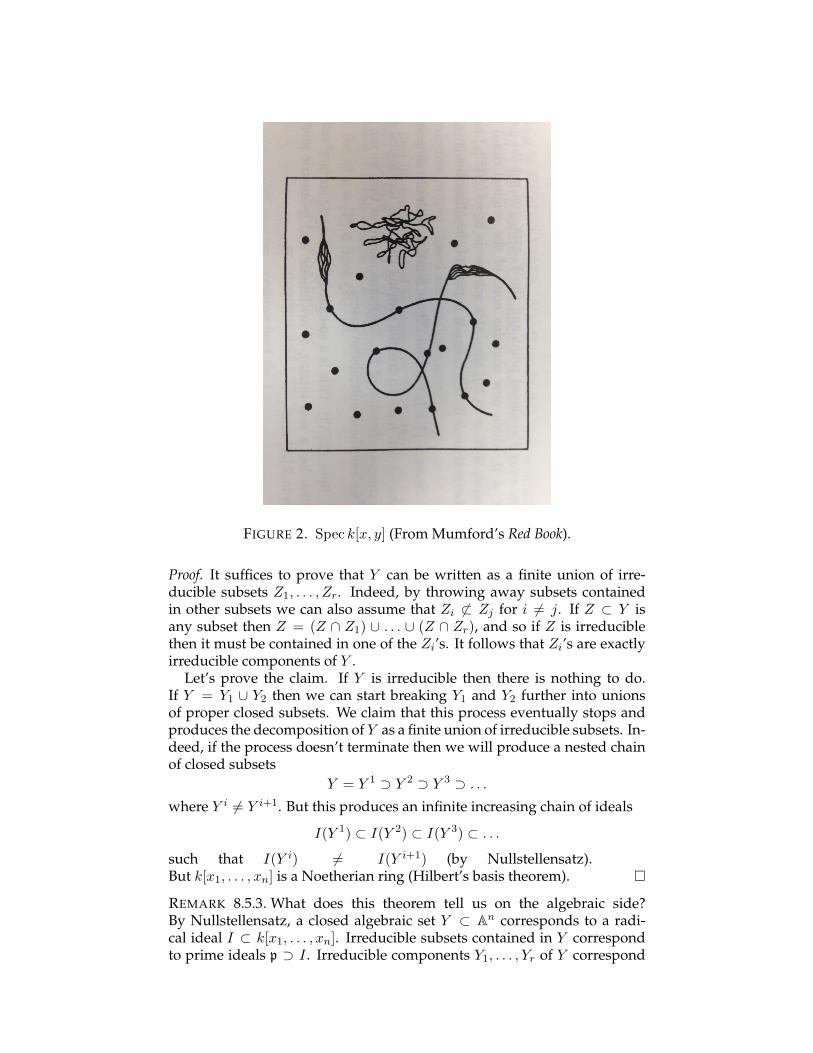
FIGURE 2. Spec k[x, y] (From Mumford’s Red Book).

Proof. It suffices to prove that Y can be written as a finite union of irre-ducible subsets Z1, . . . , Zr. Indeed, by throwing away subsets containedin other subsets we can also assume that Zi 6⇢ Zj for i 6= j. If Z ⇢ Y isany subset then Z = (Z \ Z1) [ . . . [ (Z \ Zr), and so if Z is irreduciblethen it must be contained in one of the Zi’s. It follows that Zi’s are exactlyirreducible components of Y .

Let’s prove the claim. If Y is irreducible then there is nothing to do.If Y = Y1 [ Y2 then we can start breaking Y1 and Y2 further into unionsof proper closed subsets. We claim that this process eventually stops andproduces the decomposition of Y as a finite union of irreducible subsets. In-deed, if the process doesn’t terminate then we will produce a nested chainof closed subsets

Y = Y 1 � Y 2 � Y 3 � . . .

where Y i 6= Y i+1. But this produces an infinite increasing chain of ideals

I(Y 1) ⇢ I(Y 2) ⇢ I(Y 3) ⇢ . . .

such that I(Y i) 6= I(Y i+1) (by Nullstellensatz).But k[x1, . . . , xn] is a Noetherian ring (Hilbert’s basis theorem). ⇤REMARK 8.5.3. What does this theorem tell us on the algebraic side?By Nullstellensatz, a closed algebraic set Y ⇢ An corresponds to a radi-cal ideal I ⇢ k[x1, . . . , xn]. Irreducible subsets contained in Y correspondto prime ideals p � I . Irreducible components Y1, . . . , Yr of Y correspond

to minimal (by inclusion) prime ideals p1, . . . , pr containing I . We claimthat in fact

I = p1 \ . . . \ pr.

Indeed, if f 2 pi for any i then f vanishes along each Yi, and so f 2 I .In other words, every radical ideal in k[x1, . . . , xn] is the intersection of

minimal (by inclusion) prime ideals which contain it. The same statementin fact holds in any Noetherian ring. Moreover, every ideal in a Noether-ian ring can be expressed (although not uniquely) as the intersection ofso-called primary ideals (generalization of prime ideals). This statement isknown as primary decomposition.§8.6. Affine algebraic sets. Regular functions.DEFINITION 8.6.1. Let Y ⇢ An be a closed algebraic set. The algebra of reg-ular functions on Y is the algebra of “restrictions of polynomial functions”

O(Y ) = k[x1, . . . , xn]/I(Y ).

O(Y ) is also called the coordinate algebra of Y . Another notation: k[Y ].Notice that Y is irreducible if and only if O(Y ) is a domain.

DEFINITION 8.6.2. A ring R is called reduced if its nilradicalp0 is equal to 0.

LEMMA 8.6.3. O(Y ) is a finitely generated reduced k-algebra. Moreover, anyfinitely generated reduced k-algebra is isomorphic to the algebra of the form O(Y ).Proof. Since I(Y ) is a radical ideal, the nilradical of O(Y ) is the zero ideal.Now let A be any finitely generated reduced k-algebra. Then we can writeA ' k[x1, . . . , xn]/I . We claim that I =

pI . Indeed, if x 2 p

I then x+ I is anilpotent in A, hence zero. It follows that A ' O(X), where X = V (I). ⇤DEFINITION 8.6.4. A pair (X,O(X)) of a closed algebraic set X ⇢ An andits coordinate algebra is called an affine algebraic set. An irreducible affinealgebraic set is called an affine algebraic variety.

One example is the affine space An = (kn, k[x1, . . . , n]). We can extendNullstellensatz and other previously discussed results from An to any affinealgebraic set Y as follows:COROLLARY 8.6.5. Let (Y,O(Y )) be an affine algebraic set. We have severalversions of Nullstellensatz:

(a) There is a bijection between the set of closed algebraic subsets of Y and theset of radical ideals of O(Y ) which sends Z ⇢ Y to {f 2 O(Y ) | f |Z = 0}.

(b) This bijection induces a bijection between the set of irreducible algebraicsubsets of Y and the set of prime ideals, SpecO(Y ).

(c) This bijection induces a bijection between the set of points of Y and the setof maximal ideals of O(Y ).

Closed algebraic subsets of Y are closed subsets of topology, called Zariski topology.This topology is induced by Zariski topology of An via inclusion Y ⇢ An.Proof. This follows from analogous results about An using correspondencebetween ideals of O(Y ) and ideals of k[x1, . . . , xn] containing I = I(Y ).For example, points of Y (viewed as a subset of An) correspond to maximalideals of k[x1, . . . , xn] containing I . By the first isomorphism theorem theseideals correspond to maximal ideals of O(Y ) = k[x1, . . . , xn]/I . ⇤

§8.7. Morphisms of affine algebraic sets. Given closed algebraic sets

Y1 ⇢ Anx1,...,xn

and Y2 ⇢ Amy1,...,ym

(subscripts indicate variables), how should we define maps from Y1 to Y2?

DEFINITION 8.7.1. A map ↵ : Y1 ! Y2 is called a regular morphism if ↵ is therestriction of a polynomial map

Anx1,...,xn

! Amy1,...,ym , yi = fi(x1, . . . , xn),

i.e. if there exists m polynomials f1, . . . , fm in variables x1, . . . , xn such that

↵(a1, . . . , an) = (f1(a1, . . . , an), . . . , fm(a1, . . . , an))

for any point (a1, . . . , an) 2 Y1.

EXAMPLE 8.7.2. The mapt 7! (t2, t3)

is a morphism from A1 to the cusp V (y2 � x3) ⇢ A2.

EXAMPLE 8.7.3. A morphism from A1t to the parabola X = V (y� x2) ⇢ A2,

t 7! (t, t2), and a morphism X ! A1, (x, y) 7! x, are inverses of each other.

DEFINITION 8.7.4. For any regular morphism ↵ : Y1 ! Y2, a pull-back ho-momorphism ↵⇤ : O(Y2) ! O(Y1) is defined as follows. If f 2 O(Y2) anda 2 Y1 then we simply define

(↵⇤f)(a) = f(↵(a)).

To show that ↵⇤f 2 O(Y1), we have to check that it is the restriction ofa polynomial function on An. But f itself is the restriction of a polynomialfunction f 2 k[y1, . . . , ym]. Then ↵⇤(f) is the restriction of the function

f(f1(x1, . . . , xn), . . . , fm(x1, . . . , xn)),

which is obviously a polynomial in n variables.

EXAMPLE 8.7.5. For the map

↵ : A1 ! X = V (y2 � x3) ⇢ A2, t 7! (t2, t3),

we have O(X) = k[x, y]/(x3 � y2), and

↵⇤ : k[x, y]/(x3 � y2) ! k[t], x 7! t2, y 7! t3.

The image of ↵⇤ is k[t2, t3] ⇢ k[t]. The field of fractions of k[t2, t3] is equalto k(t) and k[t] is the integral closure of k[t2, t3]. Geometrically, we say thatA1 is the normalization of the cuspidal curve X .

EXAMPLE 8.7.6. Regular morphisms between A1 and X = V (y � x2) ⇢ A2

from Example 8.7.3 induce isomorphisms

O(X) = k[x, y]/(y � x2) ' k[t] = O(A1), (x 7! t, y 7! t2), (t 7! x).

LEMMA 8.7.7. Let Mor(Y1, Y2) be the set of regular morphisms Y1 ! Y2. ThenMor(Y1, Y2) ' HomRings(O(Y2),O(Y1)), ↵ 7! ↵⇤.

In other words, a regular morphism of affine algebraic sets is completely determinedby its pull-back homomorphism, and any homomorphism of algebras of regularfunctions arises as the pull-back for some regular morphism.

REMARK 8.7.8. In the language of category theory, the category of affine al-gebraic sets and regular morphisms is equivalent to the category of finitelygenerated reduced k-algebras and homomorphisms.

Proof. If ↵ : Y1 ! Y2 is a morphism and

↵(a1, . . . , an) = (b1, . . . , bm)

for some (a1, . . . , an) 2 Y1 then bi = ↵⇤(yi)(a1, . . . , an). So ↵⇤ determines ↵.Let F : O(Y2) ! O(Y1) be any homomorphism. We have to realize it as

a pull-back homomorphism for some morphism of algebraic sets. We canconstruct a homomorphism F that fits into the commutative diagram ofhomomorphisms

O(Y2)F

> O(Y1)

k[y1, . . . , ym]

f 7! f^

F

yi 7! fi> k[x1, . . . , xn]

^

by choosing, for each i = 1, . . . ,m, a representative fi 2 k[x1, . . . , xn] of acoset F (yi). Consider a regular morphism

↵ : An ! Am, (a1, . . . , an) 7! (f1(a1, . . . , an), . . . , fm(a1, . . . , an)).

We claim that ↵(Y1) ⇢ Y2. It suffices to check that any polynomial f 2 I(Y2)vanishes on ↵(Y1), i.e. that f(f1(x1, . . . , xn), . . . , fm(x1, . . . , xn) 2 I(Y1).But modulo I(Y1) this polynomial is equal to F (f)=0. ⇤

For example, we can think about the embedding of a closed algebraic setX ⇢ An as a regular morphism X ,! An. The corresponding pull-backhomomorphism is just the canonical projection

O(An) = k[x1, . . . , xn] ! k[x1, . . . , xn]/I(X) = O(X).

And vice versa, the following proposition shows that any realization of anaffine algebraic set X as a closed algebraic subset of the affine space Am isequivalent to a choice of generators of the algebra O(X).

PROPOSITION 8.7.9. Given a choice of generators y1, . . . , ym of O(X), consider ahomomorphism k[y1, . . . , ym]

↵⇤!O(X) which sends yi to yi. Let ↵ : X ! Am bethe corresponding map. Then ↵(X) ⇢ Am is a closed algebraic set and ↵ : X !↵(X) is an isomorphism of affine algebraic sets.

Proof. By definition, X is a closed algebraic subset in some affine space An.Let Y = V (Ker↵⇤) ⇢ Am. By the first isomorphism theorem, we haveO(X) ' O(Y ). By Lemma 8.7.7, this shows that X and Y are isomorphic.Since the map X ! Y is our map ↵, we see that ↵(X) = Y is closed. ⇤

§8.8. Dominant morphisms. Let’s translate some geometry into algebra.

DEFINITION 8.8.1. A regular morphism ↵ : Y1 ! Y2 of affine algebraic setsis called dominant if its image is Zariski dense in Y2.

EXAMPLE 8.8.2. Consider projection from the hyperbola V (xy � 1) ⇢ A2

to the x-axis A1x. The image misses only 0 2 A1, so this map is dominant.

The pull-back homomorphism is

k[x] ! k[x, y]/(xy � 1) ' k

x,1

x

�

, x 7! x.

Notice that this homomorphism is injective. This is not a coincidence.

PROPOSITION 8.8.3. ↵ : Y1 ! Y2 is dominant if and only if ↵⇤ is injective.

Proof. Assume ↵ is dominant. If f 2 Ker↵⇤ then f(↵(a)) = 0 for any a 2 Y1.It follows that ↵ maps Y1 to a closed subset V (f)\Y2. Since ↵(Y1) = Y2, wehave V (f) \ Y2 = Y2, i.e. f vanishes along Y2. So f = 0.

Suppose ↵ is not dominant. Then ↵(Y1) is a proper closed subset of Y2,and therefore there exists f 2 O(Y2), f 6= 0, such that ↵(Y1) ⇢ V (f). Butthen ↵⇤(f) = 0, i.e. Ker↵⇤ 6= 0. ⇤

Homework 8

In this worksheet, we fix an algebraically closed field k. We also fix acommutative ring R (with 1).

1. Let f, g 2 C[x, y]. Suppose that f is irreducible and does not divide gin C[x, y]. (a) Show that f is irreducible and does not divide g in C(x)[y].(b) Show that V (f, g) is a union of finitely many points.

2. Let p 2 Spec k[x, y]. Show that there are exactly three possibilities:• p = {0};• p = (f), where f 2 k[x, y] is an irreducible polynomial;• p = (x� a, y � b) for some (a, b) 2 k2.

3. Let F 2 k[x1, . . . , xn] be an irreducible polynomial. Let G be a polyno-mial such that G|V (F ) = 0. Show that G is divisible by F .

4. (a) Show that Zariski topology of An has a basis of open sets of theformD(f) = {(a1, . . . , an) 2 An | f(a1, . . . , an) 6= 0} for f 2 k[x1, . . . , xn].

(b) Show that any Zariski open cover of An has a finite subcover.5. Let X ⇢ A2 be defined by the ideal I = (x2 + y2 � 1, x � 1). Is it true

that I(X) = I?6. Let X be an affine algebraic set. Consider an ideal I ⇢ O(X) and

suppose that V (I) = ;. Show that I = O(X).7. For any ideal I of R, let

V (I) = {p 2 SpecR | I ⇢ p}.(a) Show that SpecR satisfies axioms of a topological space with closedsubsets V (I). This topology is called Zariski topology. (b) Given a homo-morphism of rings f : A ! B, show that the map ↵ : SpecB ! SpecA,↵(p) = f�1(p) is continuous in Zariski topology. (c) For any f 2 R, letD(f) ⇢ SpecR be the complement of the closed set V (f). Show that setsD(f) form a base of Zariski topology, i.e. any Zariski open subset of SpecRcan be expressed as a union of open sets of the form D(f).

8. Let x, y 2 SpecR. Show that there exists either a neighborhood of xthat does not contain y or a neighborhood of y that does not contain x.

9. Let f : A ! B be a homomorphism of rings. (a) Show that in gen-eral the map ↵ : MaxSpecB ! MaxSpecA is not always well-defined.(b) If A and B are finitely generated k-algebras then ↵ is well-defined.

10. Let R be a direct product of rings R1 ⇥ . . .⇥ Rk. Show that SpecR ishomeomorphic to the disjoint union of spectra SpecR1

`

. . .`

SpecRk.11. (a) Show that the intersection of Zariski closed subsets \↵V (I↵) of

SpecR is empty if and only ifP

↵ I↵ = R. (b) Show that SpecR is quasi-compact, i.e. any open covering of SpecR has a finite sub-covering.

12. Let p ⇢ R be a prime ideal. Let I1, . . . , Ir ⇢ R be arbitrary ideals.(a) If I1\. . .\Ir ⇢ p then Ij ⇢ p for some j = 1, . . . , r. (b) If I1\. . .\Ir = pthen Ij = p for some j = 1, . . . , r.

13. Let J, I1, . . . , Ir be ideals of R such that J ⇢ I1 [ . . . [ Ir. Showthat J ⇢ Ik for some k if (a) r = 2; (b) all ideals I1, . . . , Ir are prime.(c) at most two of the ideals I1, . . . , Ir are not prime.

§9. LOCALIZATION AND LOCAL RINGS

§9.1. Examples from number theory and geometry.

EXAMPLE 9.1.1 (Number Theory). A typical example of localization is a for-mation of rational numbers as fractions of integers: Z ⇢ Q. But there aremany other intermediate subrings between Z and Q formed by fractionswith some condition on denominators. For example, we can invert only 2:

Z[1/2] =n a

2n| a 2 Z, n � 0

o

.

A principal ideal (2) is maximal in Z but in Z[1/2] it gives the whole ring.Or we can invert everything coprime to 2 (i.e. odd):

Z(2) =na

b| a, b 2 Z, b 62 (2)

o

.

This ring has only one maximal ideal, namely a principal ideal (2). Indeed,any element not in this ideal is invertible. This an example of a local ring:

DEFINITION 9.1.2. A ring is called local if it has only one maximal ideal.

In general, localization of the ring gives a ring with a simplified idealstructure: any ideal containing one of the denominators disappears.

EXAMPLE 9.1.3 (Geometry). In geometry we often study spaces locally in aneighborhood of a point. What are these neighborhoods in algebraic ge-ometry? Consider the affine line A1 with ring of functions k[x]. Zariskineighborhoods of the origin 0 2 A1 have form

U = A1 \ {↵1, . . . ,↵r}, ↵i 6= 0 for any i.

What are the functions on this neighborhood? We are algebraists, so we areinterested in polynomial or rational functions defined in U , and so we take

O(U) :=

⇢

p(x)

(x� ↵1)n1 . . . (x� ↵r)nr

�

�

�

p(x) 2 k[x]

�

⇢ k(x)

= k

x,1

x� ↵1, . . . ,

1

x� ↵r

�

,

the ring obtained from k[x] by inverting x� ↵1, . . . , x� ↵r.We can go further and invert all polynomials that don’t vanish at 0:

k[x](x) =

⇢

f(x)

g(x)

�

�

�

g 62 (x)

�

⇢ k(x).

This gives functions defined in some Zariski neighborhood of 0. The neigh-borhood depends on function: we have to throw away all roots of the de-nominator g(x). The ring k[x](x) is local: the only maximal ideal left is theprincipal ideal of x. A useful intuition in algebraic geometry is to thinkabout k[x](x) as functions on a small “local” neighborhood of 0 2 A1, eventhough there is no Zariski neighborhood that can be used for that purpose.

§9.2. Localization of rings.

DEFINITION 9.2.1. A subset S ⇢ R is called a multiplicative system if• If s, t 2 S then st 2 S.• 1 2 S, 0 62 S.

A localization S�1R is the set of equivalence classes of fractionsnr

s

�

� r 2 R, s 2 So

.

Two fractions r/s and r0/s0 are equivalent if there exists t 2 S such thatt(s0r � sr0) = 0. (9.2.1)

The ring structure on S�1R is defined using usual addition and multiplica-tion of fractions. One has to check that these operations are well-defined.We have a homomorphism

R ! S�1R, r 7! r

1.

If R is not a domain then this homomorphism is not necessarily injective.

REMARK 9.2.2. If R is a domain then without loss of generality we cantake t = 1 in (9.2.1), but in general we have to modify the usual cross-multiplication formula. This is because we want any t 2 S to become in-vertible in S�1R. Suppose that ta = 0 in R for some a 2 R. Then we shouldhave ta

1 = 0 in S�1R. Since t1 is invertible, we should be able to conclude

that a1 = 0, i.e. that fractions a

1 and 01 are equivalent. And according to our

definition they are because t(1 · a� 0 · 1) = 0. We also see that it is possiblethat a 6= 0 in R but a

1 = 0 in S�1R.

LEMMA 9.2.3. The ring S�1R is well-defined.

Proof. A tedious calculation. ⇤EXAMPLE 9.2.4. If R is a domain then S = R\{0} is a multiplicative system.The localization S�1R is the quotient field of R. More generally, for anyring R, we can take S to be the set of all non-zerodivisors. The localizationS�1R is called a total ring of fractions.

EXAMPLE 9.2.5. Suppose x 2 R is not a nilpotent element. Then

S = {1, x, x2, x3, . . .}is a multiplicative system. The localization S�1R is often denoted by R

⇥

1x

⇤

.

Here is perhaps the most important example of localization:

DEFINITION 9.2.6. Let p ⇢ R be a prime ideal, i.e.if xy 2 p then either x 2 p or y 2 p.

A contrapositive of this statement shows that S = R \ p is a multiplicativesystem. The corresponding localization S�1R is denoted by Rp and calledthe localization of R at p.

EXAMPLE 9.2.7. Take a prime ideal (x) ⇢ k[x], the ideal of polynomial func-tions that vanish at 0 2 A1. Then k[x](x) is the ring of all rational functionsof the form f(x)

g(x) such that g(x) 62 (x), i.e. such that g(0) 6= 0.

§9.3. Extension and contraction of ideals in R and S�1R. .

DEFINITION 9.3.1. Let f : A ! B be a homomorphism of rings. For anyideal J ⇢ B, the ideal f�1(J) of A is called a contraction of J . For any idealI ⇢ A, the ideal Bf(I) of B is called an extension of I (notice that f(I) itselfis almost never an ideal unless f is surjective).

Applying this construction for the localization gives

DEFINITION 9.3.2. For any ideal I ⇢ R, its extension S�1I ⇢ S�1R is thesubset of fractions of the form x

s with x 2 I , s 2 S. Let f : R ! S�1R bethe canonical map. If J ⇢ S�1R is an ideal then its contraction f�1(J) ⇢ R,abusing notation, it is often denoted by J \R.

PROPOSITION 9.3.3. We have the following properties:• The mapping I 7! S�1I is a 1 : 1 mapping of the set of all contracted

ideals of R (i.e. ideals of the form R \ J) to the set of all ideals of S�1R.• Prime ideals of S�1R are in 1 : 1 correspondence (p $ S�1p) with prime

ideals of R that don’t intersect S.

Proof. Let J ⇢ S�1R be an ideal and let r/s 2 J . Then r = s(r/s) 2 J , andtherefore r 2 R \ J . It follows that J ⇢ S�1(R \ J). The other inclusion isobvious, and so we have

J = S�1(R \ J).

This proves the first part.For the second part, if I ⇢ R is any ideal that intersects S then of course

S�1I = R�1S. We claim that if p ⇢ R is a prime ideal that does not inter-sect S then S�1p is also prime. Indeed, suppose we have

r

s

r0

s0=

x

t,

where x 2 p. Then u(trr0 � xss0) = 0 for some u 2 S. It follows thattrr0 � xss0 2 p, and therefore trr0 2 p. This implies that r or r0 is in p, i.e.rs or r0

s0 is in S�1p. In the other direction, if J ⇢ S�1R is a prime ideal thenR\ J is also a prime ideal. This is true for any homomorphism f : A ! B:if J ⇢ B is a prime ideal then f�1(J) ⇢ A is also a prime ideal. ⇤

In the language of spectra, the homomorphism R ! S�1R induces aninjective map of spectra SpecS�1R ,! SpecR. The image consists of primeideals which do not intersect S.

LEMMA 9.3.4. Rp is a local ring with a maximal ideal pp (extension of p).

Proof. We will use the following simple observation: If A is a local ringwith a maximal ideal m then any x 62 m is not contained in a proper idealand therefore is invertible. Elements in m are of course not invertible. Andthe other way around, if A⇤ ⇢ A is the set of invertible elements (units) andm = A\A⇤ happens to be an ideal of A then A is a local ring with a maximalideal m, because any proper ideal does not intersect A⇤.

Returning to Rp, let m be the extension of the ideal p. This is a properideal by the previous proposition. But any element not in m has form r/swith r, s 62 p, which is obviously invertible in Rp. So Rp is a local ring. ⇤

Localization is used when we want to focus on ideals disjoint from S.We give two examples of using this idea in arguments.

§9.4. Nilradical.

PROPOSITION 9.4.1. Let R be a commutative ring. The intersection of all itsprime ideals is equal to the set of nilpotent elements (called the nilradical) of R:

\

p2SpecRp = {x 2 R |xn = 0 for some n > 0}.

Proof. If p is a prime ideal and xn = 0 for some n then xn 2 p and thereforex 2 p. Now suppose that x is not nilpotent. Then

S = {1, x, x2, . . . }is a multiplicative system. Consider the localization S�1R and any maxi-mal (and hence prime) ideal I of it. Then p = R \ I is a prime ideal of Rthat does not intersect S, and therefore does not contain x. ⇤

§9.5. Going-up Theorem.

THEOREM 9.5.1 (Going-up Theorem). Let A ⇢ B be rings and suppose that Bis integral over A. Then the pull-back map SpecB ! SpecA is surjective.

Proof. We have to show that for any prime ideal p ⇢ A, there exists a primeideal q ⇢ B such that

p = q \A.

Let S ⇢ A be a complement of p. We can view S as a multiplicative systemnot only in A but also in B. Localizing at S gives a commutative diagram

B↵> S�1B

A

^

�> Ap

^(9.5.1)

where the vertical arrows are inclusions. Notice that S�1B is integral over Ap:if b 2 B is a root of a monic polynomial

bn + a1bn�1 + . . .+ an = 0

then b/s for s 2 S is a root of a monic polynomial

(b/s)n + (a1/s)(b/s)n�1 + . . .+ (an/s

n) = 0.

Suppose we can prove the theorem for Ap ⇢ S�1B. Then there exists aprime ideal J of S�1B such that J \ Ap = S�1p. Let q = ↵�1(J). We claimthat q \A = p. This follows from commutativity of the diagram (9.5.1) andbecause ��1(S�1p) = p by Prop. 9.3.3.

It remains to consider the case when A is a local ring with a maximalideal m. Let m0 ⇢ B be any maximal ideal. We claim that m0 \ A = m. In

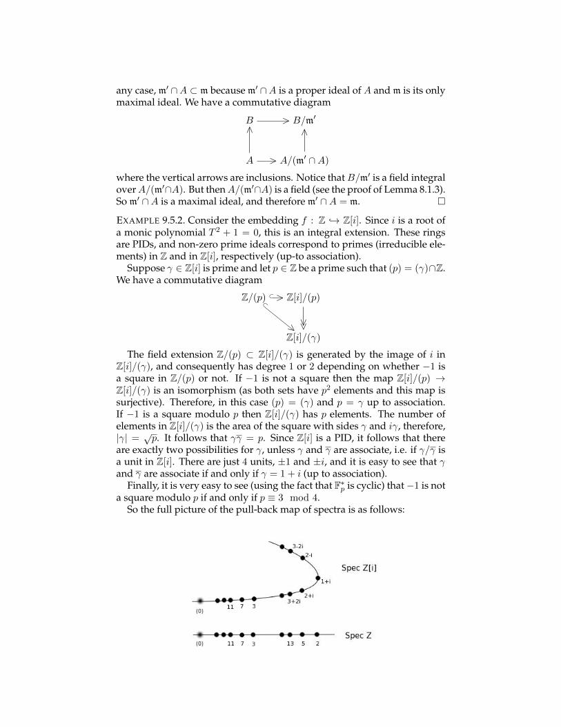
any case, m0 \A ⇢ m because m0 \A is a proper ideal of A and m is its onlymaximal ideal. We have a commutative diagram

B > B/m0

A

^

> A/(m0 \A)

^

where the vertical arrows are inclusions. Notice that B/m0 is a field integralover A/(m0\A). But then A/(m0\A) is a field (see the proof of Lemma 8.1.3).So m0 \A is a maximal ideal, and therefore m0 \A = m. ⇤EXAMPLE 9.5.2. Consider the embedding f : Z ,! Z[i]. Since i is a root ofa monic polynomial T 2 + 1 = 0, this is an integral extension. These ringsare PIDs, and non-zero prime ideals correspond to primes (irreducible ele-ments) in Z and in Z[i], respectively (up-to association).

Suppose � 2 Z[i] is prime and let p 2 Z be a prime such that (p) = (�)\Z.We have a commutative diagram

Z/(p) ⇢ > Z[i]/(p)

Z[i]/(�)__

⇢

>

The field extension Z/(p) ⇢ Z[i]/(�) is generated by the image of i inZ[i]/(�), and consequently has degree 1 or 2 depending on whether �1 isa square in Z/(p) or not. If �1 is not a square then the map Z[i]/(p) !Z[i]/(�) is an isomorphism (as both sets have p2 elements and this map issurjective). Therefore, in this case (p) = (�) and p = � up to association.If �1 is a square modulo p then Z[i]/(�) has p elements. The number ofelements in Z[i]/(�) is the area of the square with sides � and i�, therefore,|�| = p

p. It follows that �� = p. Since Z[i] is a PID, it follows that thereare exactly two possibilities for �, unless � and � are associate, i.e. if �/� isa unit in Z[i]. There are just 4 units, ±1 and ±i, and it is easy to see that �and � are associate if and only if � = 1 + i (up to association).

Finally, it is very easy to see (using the fact that F⇤p is cyclic) that �1 is not

a square modulo p if and only if p ⌘ 3 mod 4.So the full picture of the pull-back map of spectra is as follows:

§9.6. Finite morphisms. Now let’s translate some algebra into geometry.

DEFINITION 9.6.1. A morphism of affine algebraic sets X ! Y is calledfinite if O(X) is integral over O(Y ) via the pull-back O(Y ) ! O(X).

EXAMPLE 9.6.2. This gives a geometric way to reformulate Noether’s nor-malization lemma: any closed algebraic set X admits a dominant finitemorphism to An for some n. Moreover, the proof in §7.4 gives the follow-ing more accurate statement: if X ⇢ Am is a closed algebraic subset thenwe can choose a direct sum decomposition of vector spaces Am = An � Ar

such that the projection of X onto An along Ar is a finite morphism.

THEOREM 9.6.3. Any dominant finite morphism is surjective and has finite fibers.

Proof. Let ↵ : X ! Y be a dominant finite morphism. Let A = O(X)and let B = O(Y ). By Lemma 8.8.3, we can identify B with a subring ofA via the pull-back homomorphism. By definition of a finite morphism,A is integral over B. Let y 2 Y . It corresponds to a maximal ideal m ⇢ B.To show that ↵ is surjective, we have to check that there exists a maximalideal n ⇢ A such that n \ B = m and to show that ↵ has finite fibers, wehave to check that there are only finitely many possible n’s. By the going-up theorem, we can find a prime ideal p ⇢ A such that p\B = m. But thenA/p is a domain integral over a field k = B/m, and so A/p is also a field,and so p is in fact a maximal ideal.

There is a natural bijection between the set of maximal ideals n ⇢ Asuch that n \ B = m and MaxSpecA/Am. The algebra A/Am is finitelygenerated and integral over B/m = k, and so is a finitely generated k-module, i.e. a finite-dimensional vector space. Since any ideal of A/Am isa vector subspace, we see that A/Am satisfies a descending chain conditionfor ideals. So it is enough to prove Lemma 9.6.5 below. ⇤

DEFINITION 9.6.4. A ring R is called Artinian if it satisfies d.c.c. for ideals.

LEMMA 9.6.5. Any Artinian ring R has the following properties:• Any prime ideal of R is maximal.• R has only finitely many maximal ideals.

Proof. For the first statement, if p ⇢ R is a prime ideal then R/p is an Ar-tinian domain. For any x 2 R/p, the sequence

(x) � (x2) � (x3) � . . .

stabilizes, and therefore xn = xn+1y for some n and for some y 2 R/p, butthis implies that 1 = xy. So R/p is a field and p is maximal.

For the second statement, consider the set of finite intersections of maxi-mal ideals. By d.c.c, this set has the minimal element, i.e. there exist maxi-mal ideals m1, . . . ,mr ⇢ R such that

m \m1 \ . . . \mr = m1 \ . . . \mr

for any maximal ideal m, or equivalently

m1 \ . . . \mr ⇢ m.

We claim that this implies that m = mi for some i. If not, then each mi

contains xi such that xi 62 m. But then

x1 . . . xr 2 m1 \ . . . \mr ⇢ m,

and since m is prime, one of the xi’s is contained in m, contradiction. ⇤EXAMPLE 9.6.6. Consider projection ↵ of the parabola X = V (y � x2) ⇢ A2

onto the y-axis Y = A1y. The pull-back homomorphism ↵⇤ is

k[y] = O(Y ) ! O(X) = k[x, y]/(x2 � y) ' k[x], y 7! x2.

Since x is a root of a monic polynomial T 2 � y, O(X) is integral over O(Y ),and so ↵ is a finite morphism. The preimage of any point a 2 A1

y is obvi-ously ±p

a, i.e. either one (if a = 0) or two (if a 6= 0) points. Analysis usedin the proof of Theorem 9.6.3 gives us a bit more: points in the preimage ofa 2 A1

y correspond to maximal ideals of the Artinian k-algebra

k[x]/(x2 � a) '(

k[x](x�p

a)� k[x]

(x+pa)

' k � k if a 6= 0

k[x]/(x2) = {a+ b✏ | a, b 2 k, ✏2 = 0} if a = 0

The algebra k[x]/(x2) is known as the algebra of dual numbers. It has onlyone maximal ideal (✏). However, this algebra is 2-dimensional as a vectorspace over k, just like the algebra k � k. This reflects our intuition that thepreimage of 0 should be one point but counted with multiplicity 2.

§9.7. Localization of modules. Localization of rings R 7! S�1R can begeneralized to localization of modules.

DEFINITION 9.7.1. Let M be an R-module and let S ⇢ R be a multiplicativesystem. We define S�1M as the set of equivalence classes of fractions m/s,where m 2 M , s 2 S. Two fractions m/s and m0/s0 are called equivalent ifthere exists t 2 S such that

t(s0m� sm0) = 0.

We make S�1M into an S�1R-module by declaring that r/s 2 S�1R actson m/t 2 S�1M by sending it to (rm)/(st).

REMARK 9.7.2. Even when R is a domain, it can of course happen thattm = 0 for some t 2 S, m 2 M \ {0}. Then m/1 should be equal to 0in S�1M because t is invertible in S�1R. This explains appearance of t inthe definition of equivalent fractions.

NOTATION 9.7.3. If p 2 SpecR and S = R \ p then S�1M is denoted by Mp.

LEMMA 9.7.4. Localization of modules is well-defined.

Proof. A tedious calculation. ⇤LEMMA 9.7.5. Localization is a special case of extension of scalars:

S�1M ' S�1R⌦R M.

Proof. Consider a bilinear map of R modules

S�1R⇥M ! S�1M,⇣r

s,m⌘

7! rm

s.

It induces a surjective map of R-modules

: S�1R⌦R M ! S�1M.

Why is it injective? Any element of S�1R⌦R M can be written asX

i

risi

⌦mi =X

i

tiris

⌦mi (where s =Q

jsj and ti =

Q

j 6=i

sj)

=X

i

1

s⌦ tirimi =

1

s⌦m (where m =

P

itirimi).

If 0 = (1s ⌦m) = ms then tm = 0 for some t 2 S. But then

X

i

risi

⌦mi =1

s⌦m =

t

ts⌦m =

1

ts⌦ tm = 0.

So is injective. ⇤

§9.8. Localization is exact.

LEMMA 9.8.1. If0 ! M ! N ! K ! 0

is an exact sequence of R-modules then

0 ! S�1M ! S�1N ! S�1K ! 0

is an exact sequence of S�1R-modules. In particular, if M ⇢ N then we can viewS�1M as a submodule of S�1N .

Proof. Any extension of scalars, and more generally tensoring with any R-module, is right-exact. So

S�1M ! S�1N ! S�1K ! 0

is exact. It remains to show that if M ��!N is injective then S�1M �!S�1N

is also injective. If (ms ) =�(m)s = 0 in S�1N then t�(m) = �(tm) = 0 for

some t 2 S. But then tm = 0 in M and therefore ms = 0 in S�1M . ⇤

REMARK 9.8.2. We can view the second sequence of the lemma as the firstsequence tensored with S�1R. In the language of flat modules, the lemmasays that S�1R is a flat R-module.

§9.9. Nakayama’s Lemma. Nakayama’s Lemma is usually used in the fol-lowing form:

LEMMA 9.9.1 (Nakayama’s Lemma - I). Let R be a local ring with a maximalideal m and let M be a finitely generated R-module. Let s1, . . . , sn 2 M . If theseelements generate M modulo mM then in fact they generate M .

This follows from

LEMMA 9.9.2 (Nakayama’s Lemma - II). Let R be a local ring with a maximalideal m and let M be a finitely generated R-module. If mM = M then M = 0.

Indeed, let N be a submodule of M generated by s1, . . . , sn. Then weare given that M = N + mM , i.e. that M/N = m(M/N). We deduce thatM/N = 0, i.e. that M = N .

To prove version II, we are going to use the “adjoint matrix/determinant”trick we used to show that x 2 B is integral over a subring A ⇢ B if andonly if x is contained in a finitely generated A-submodule of B.

We will prove a slightly more general result. Let R be any ring and letM be a finitely generated R-module. Claim: if I is an ideal contained in allmaximal ideals and IM = M then M = 0.

Let m1, . . . ,mk be generators of M . We have

mi =X

aijmj , where aij 2 I.

ThenX

j

(�ij � aij)mj = 0

for any i. Multiplying by the adjoint matrix, we see thatamj = 0 for any j,

where a = det(�ij � aij) can be written as 1+ x, where x 2 I . We claim thata is invertible, and therefore

mj = a�1(amj) = 0 for any j,

and therefore M = 0. If a is not invertible then it belongs to some maximalideal m ⇢ R. But x 2 I ⇢ m, and so 1 = a� x 2 m, a contradiction.

Homework 9

Let R be a commutative ring (with 1).1. (a) Show that the nilradical of R is a prime ideal if and only if SpecR

contains a “generic point” ⌘, i.e. a point such that ⌘ = SpecR. (b) LetI ⇢ R be an ideal. Show that p

I =\

p2SpecR

I⇢p

p.

2. Let � : A ! B be a homomorphism of rings. Construct a bijection{contracted ideals in A} $ {extended ideals in B}.

3. Let R be a ring and let ⌃ be the set of its multiplicative systems. Showthat ⌃ contains maximal (by inclusion) subsets and that S 2 ⌃ is maximalif and only if R \ S is a minimal (by inclusion) prime ideal.

4. Let A ⇢ B be domains. Suppose B \A is multiplicatively closed in B.Show that A is integrally closed in B.

5. Let R be a ring and let p ⇢ R be a prime ideal. (a) Show that thelocalization Rp is a field if and only if for any element x 2 p there existsy 62 p such that xy = 0. (b) Find an example of a commutative ring R anda prime ideal p 6= 0 such that Rp is a field.

6. Let R be a ring with only finitely many maximal ideals. Suppose thatfor each maximal ideal m ⇢ R, Rm is Noetherian. Prove that (a) the prod-uct of localization maps R 7!Q

mRm is an embedding; (b) R is Noetherian.

7. Consider the following ideal

P = (2, 1 +p�5) ⇢ R = Z[

p�5].

(a) Show that P is maximal but not principal. (b) Show that the extendedideal PP ⇢ RP is principal.

8. Let A ⇢ B be rings, B is integral over A. Let p1 ⇢ . . . ⇢ pn be a chain ofprime ideals of A and let q1 ⇢ . . . ⇢ qm (m < n) be a chain of prime idealsof B such that qi \B = pi for i m. Then the q-chain can be extended to achain q1 ⇢ . . . ⇢ qn such that qi \B = pi for all i.

9. Show that the ring R is reduced if and only if Rp s reduced for anyprime ideal p ⇢ R.

10. Let R be a domain and let I ⇢ R be an ideal. An element x 2 R iscalled integral over I if it satisfies an equation of the form xn + a1xn�1 +. . . + an = 0 with ak 2 Ik, the k-th power of the ideal I , for each k � 1.Show that x is integral over I if and only if there exists a finitely generatedR-module M , not annihilated by any element of R, such that xM ⇢ IM .

11. Let R be a ring. Let M1 and M2 be submodules of an R-module N .

(a) (S�1M1) + (S�1M2) = S�1(M1 +M2);

(b) (S�1M1) \ (S�1M2) = S�1(M1 \M2);

(c) if M1 � M2 then S�1(M1/M2) ' (S�1M1)/(S�1M2).

12. Let R be a ring. Let M be a finitely generated R-module. Show that

S�1(AnnM) ' Ann(S�1M).

§10. BONUS SECTION: A BIT MORE ALGEBRAIC GEOMETRY

§10.1. Rational functions.

DEFINITION 10.1.1. Let X be an affine variety. The field of fractions k(X) ofthe domain O(X) is called the field of rational functions on X . For example,

k(An) = k(x1, . . . , xn).

Any rational function f 2 k(X) can be written as a ratio of 2 regular func-tions p, q 2 O(X). It can be thought of as a function X \ V (q) ! k.

DEFINITION 10.1.2. A rational function f 2 k(X) is called regular at x 2 X ifit can be written as p/q such that q(x) 6= 0. In terms of the the correspondingmaximal ideal m ⇢ O(X), functions regular at x form a local ring O(X)m.

REMARK 10.1.3. If O(X) is not a UFD then fractions cannot be written inlowest terms, and it is not always obvious if f 2 k(X) is regular at x 2 X .For example, consider the quadric cone

X = V (xy � z2) ⇢ A3.

We claim that x/z 2 k(X) is regular at p = (0, 1, 0) 2 X even thoughz(p) = 0. Indeed, in k(X) we have x/z = z/y and y(p) 6= 0.

PROPOSITION 10.1.4. Let X be an affine algebraic variety. Let f 2 k(X). Thenf is regular at any point x 2 X if and only if f 2 O(X).

Proof. One direction is obvious. Suppose f is regular at any point x 2 X ,i.e. we can write f = p

x

qx

, where qx(x) 6= 0. Consider an ideal I ⇢ O(X)

generated by qx for x 2 X . Since V (I) = ;,pI = O(X) by Nullstellensatz6.

It follows that 1 2 I , i.e. we can write

1 = a1qx1 + . . .+ arqxr

for some x1, . . . , xr 2 X.

It follows that

f = fa1qx1 + . . .+ farqxr

=px1

qx1

a1qx1 + . . .+px

r

qxr

arqxr

=

= px1a1 + . . .+ pxr

ar 2 O(X).

This idea is known as “algebraic partition of unity” trick. ⇤§10.2. Dimension. There are two ways to think about dimension:

• Dimension is the number of independent parameters needed to spec-ify a point. For example, our space is three-dimensional because weneed three coordinates, x, y, and z.

• Dimension of space is 1 plus maximal dimension of its subspace.For example, our space is three-dimensinal because it contains flags

{point} ⇢ {curve} ⇢ {surface} ⇢ {space}In Algebraic Geometry, these ideas can be made rigorous:

DEFINITION 10.2.1. Let X be an affine variety. We define

dimX := tr.deg.k k(X).

6We proved Nullstellensatz for O(An

). The general case is treated in the homework.

DEFINITION 10.2.2. Let R be any ring. We define its Krull dimension dimR asthe maximal number r (possibly 1) such that R contains a chain of primeideals of length r + 1:

p0 ( p1 ( . . . ( pr. (10.2.1)

THEOREM 10.2.3. Let X be an affine variety. Then

dimX = dimO(X).

Proof. Since O(X) is a finitely generated k-algebra, it is integral over apolynomial subalgebra k[y1, . . . , yn], by Noether’s Normalization Lemma.Then k(X)/k(y1, . . . , yn) is an algebraic field extension, and we have

dimX = tr.deg.k k(X) = tr.deg.k k(y1, . . . , yn) = n.

Next we would like to show that

dimO(X) = dim k[x1, . . . , xn]. (10.2.2)

Let (10.2.1) be any chain of prime ideals in O(X). Then qi := pi\k[x1, . . . , xn]are prime ideals in k[x1, . . . , xn]. We claim that qi 6= qi+1 for any i. Indeed,suppose qi = qi+1. Then B := O(X)/pi is integral over A := k[x1, . . . , xn]/qi.Let S = A \ {0}. Then S�1B is integral over S�1A, which is the field offractions of A. By the standard lemma, it follows that S�1B is also a field.However, S�1pi+1 is its proper ideal, contradiction. Next take any chain

q0 ( q1 ( . . . ( qs

of prime ideals in k[x1, . . . , xn]. By the Going-up Theorem7, we can lift thischain to the chain

p0 ( p1 ( . . . ( ps

of prime ideals in O(X). The formula (10.2.2) follows. At this point every-thing is reduced to showing that

dim k[x1, . . . , xn] = n.

Existence of the chain of prime ideals

0 ( (x1) ( (x1, x2) ( . . . ( (x1, . . . , xn)

shows that dim k[x1, . . . , xn] � n. For an opposite inequality, consider achain of prime ideals

p0 ( p1 ( . . . ( ps ⇢ k[x1, . . . , xn].

It gives a chain of affine varieties

V (ps) ( V (ps�1) ( . . . ( V (p0) ⇢ An.

Since dimAn = n, it suffices to prove the following Lemma 10.2.4. ⇤

LEMMA 10.2.4. Let X ⇢ Y be affine varieties. Then dimX dimY . Moreover,if X 6= Y then dimX < dimY .

7In our version of the Going-up Theorem, we showed how to lift one prime ideal.For this slightly more general version, see the homework.

Proof. The affine variety Y is a closed algebraic subset of ANt1,...,t

N

.Let n = dimY . Since O(Y ), and therefore k(Y ), is generated by restrictionsof t1, . . . , tN , any n + 1 of these restrictions are algebraically dependent.The same is true for their restrictions on X , and therefore dimX n.

Now let’s suppose that dimX = n. Then some n of the coordinates arealgebraically independent in k(X), and therefore also in k(Y ). Withoutloss of generality we can assume that restrictions of t1, . . . , tn are these al-gebraically independent coordinates. If X 6= Y then we can find a non-zerou 2 O(Y ) such that u|X = 0. Since u is algebraic over k(t1, . . . , tn), we havethe following identity along Y :

a0um + . . .+ am = 0, where ai 2 k[t1, . . . , tn] for i = 0, . . . ,m.

We can assume that am(t1, . . . , tn) is a non-vanishing polynomial (other-wise divide this identity by u). But since u|X = 0, we have am|X = 0.But t1, . . . tn are algebraically independent in O(X), a contradiction. ⇤§10.3. Discrete Valuation Rings. Domains of Krull dimension 0 are fields.How to characterize domains R with dimR = 1? In these domains everynon-zero prime ideal is maximal, for example any PID such as Z or k[x].More generally, Noetherian integrally closed domains of Krull dimension 1are called Dedekind domains. For example, any ring of algebraic integersand any coordinate ring of an affine algebraic curve are Dedekind domains.A satisfactory structure theory of these rings is available, but we are onlygoing to focus on the local case.

DEFINITION 10.3.1. A discrete valuation of a field K is a function v : K⇤ ! Zsuch that

• v(xy) = v(x) + v(y);• v(x+ y) � min(v(x), v(y));• v(K⇤) = Z.

The subring R = {x 2 K | v(x) � 0 is called the valuation ring of v.A domain R is called a DVR (Discrete Valuation Ring) if its field of frac-

tions has a discrete valuation such that R is its valuation ring.

EXAMPLE 10.3.2. The localization Z(p) is a DVR. Indeed, let’s define a func-tion v : Q⇤ ! Z as follows: v(x) = n if x = pn a

b , where a, b 2 Z are coprimeto p. All properties of a discrete valuation can be immediately checked.Notice that v(x) � 0 if and only if x can be written as a

b where a, b 2 Z andb is coprime to p, i.e. if and only if x 2 Z(p). More generally, this construc-tion shows that R(f) is a DVR for any irreducible element f of a UFD R.Example: k[x](x�a) for any a 2 k.

LEMMA 10.3.3. Let v be any discrete valuation of a field K. Its valuation ring Ris a local ring with maximal ideal m = {x 2 R | v(x) > 0} and field of fractionsK.

Proof. R is a ring. Indeed, if v(x), v(y) � 0 then v(xy) = v(x) + v(y) � 0and v(x+ y) � min(v(x), v(y)) � 0. Since v(1) = v(1 · 1) = v(1) + v(1), wehave v(1) = 0. So R is a ring with unity.

Let x 2 K. If v(x) � 0 then x 2 R. If v(x) < 0 then x�1 2 R becausev(x�1) = v(1)� v(x) > 0. It follows that K is the field of fractions of R.

To show that m is an ideal of R, suppose that r 2 R and x, y 2 m. Thenv(rx) = v(r) + v(x) > 0 and v(x + y) � min(v(x), v(y)) > 0. Therefore,rx 2 m and x+ y 2 m.

If x 2 R and v(x) = 0 then v(x�1) = �v(x) = 0, and therefore x is a unitin R. If v(x) > 0 then x 2 m. So R is a local ring with maximal ideal m (seethe proof of Lemma 9.3.4). ⇤

The following theorem gives a nice characterization of DVRs. In thecourse of the proof we will discover other interesting things about DVRs.

THEOREM 10.3.4. Let R be a ring. TFAE:(1) R is a DVR.(2) R is a Noetherian, integrally closed, local domain of Krull dimension 1.

Proof. Let R be a DVR. We already know that R is a local domain withmaximal ideal m.

Let t 2 m be any element such that v(t) = 1. We claim that m = (t).More generally, we claim that any ideal I of R has form (tn), where n isthe minimal integer such that I contains an element x such that v(x) = n.Indeed, since v(tn/x) = 0, tn/x is a unit in R, and therefore tn and x areassociate, and in particular tn 2 I . If y 2 I then v(y) � n, and thereforev(y/tn) � 0 and so y/tn 2 R. It follows that I = (tn).

Calculations of the previous paragraph show, in particular, that R is aPID and therefore is integrally closed and has Krull dimension 1.

Now let’s fix a Noetherian, integrally closed, local domain R of Krulldimension 1. Let m 2 R be its only maximal ideal. Let

I =\

n�1

mn.

Since R is Noetherian, I is a finitely generated R-module. Since I = mI ,in fact I = 0 by Nakayama’s lemma.

CLAIM 10.3.5. The maximal ideal m is principal, m = (t).

Given the claim, let’s show that R is a DVR. Let x 2 R. Since I = 0,we can find an integer n such that x 2 mn = (tn) but x 62 mn+1 = (tn+1).It follows that x = tnu, where u 62 m, i.e. u is a unit of R. It follows thatany x 2 K⇤ can be written as tnu, where n 2 Z and u 2 R is a unit. Thisexpression is unique, and therefore we can define a function v : K⇤ ! Z,v(x) = n. It is straightforward to check all axioms of the valuation.

Let’s prove the claim. By Nakayama’s lemma, m 6= m2. Let t 2 m \ m2.Since dimR = 1, m is the only non-zero prime ideal of R. It follows that

m =p

(t).

This implies that mn ⇢ (t) for some n. Indeed, since R is Noetherian, mhas finitely many generators x1, . . . , xr and we can choose N > 0 such thatxNi 2 (t) for any i. Then y1 . . . ym 2 (t) for any y1, . . . , ym 2 m as long asm > r(N � 1). Let n be the integer such that mn ⇢ (t) but mn�1 6⇢ (t). Letb 2 mn�1 \ (t). Let x = t/b 2 K. Then x�1 62 R (since b 62 (t)). Since Ris integrally closed, x�1 is not integral over R. It follows that x�1m 6⇢ m(since m is a finitely generated R-module). But x�1m ⇢ R (since if z 2 m

then bz 2 mn ⇢ (t) and therefore x�1z 2 R). It follows that x�1m = R,i.e. that m = (x). ⇤

Homework 10Let R be a commutative ring (with 1). Let k be an algebraically closed

field.1. Let R be a ring. Let M1 and M2 be R-modules. Show that

S�1(M1 ⌦R M2) ' (S�1M1)⌦S�1R (S�1M2).

2. Let R be a ring. Let M be an R-module. Show that M = 0 if and onlyif Mm = 0 for any maximal ideal m ⇢ R.

3. Show that Nakayama’s Lemma fails if the module M is not assumedto be finitely generated.

4. Let M and N be finitely generated modules over a local ring R. Showthat if M ⌦R N = 0 then either M = 0 or N = 0.

5. Let M and N be finitely generated modules over a local ring R. Showthat if M ⌦R N ' R then M ' R and N ' R.

6. Let ↵ : A2 ! A2 be a morphism given by polynomials f, g 2 k[x, y].(a) Show that if ↵ is an isomorphism then the polynomial

det

"

@f(x,y)@x

@g(x,y)@x

@f(x,y)@y

@g(x,y)@y

#

is a nonzero constant (the converse of this is a famous open problem calledthe Jacobian Conjecture). (b) Give an example when ↵ is an isomorphismbut polynomials f, g are not both linear polynomials.

7. Is a hyperbola V (xy � 1) ⇢ A2 isomorphic to A1?8. Consider the morphism A2 ! A2 defined by formulas (x, y) 7! (x, xy).

Is the image Zariski closed? Zariski open? Zariski dense?9. Consider the morphism ↵ : A1 ! An given by t 7! (t, t2, . . . , tn). Show

that ↵ induces an isomorphism between A1 and V (I), where I is generatedby 2⇥ 2 minors of the following matrix

1 x1 x2 . . . xn�1

x1 x2 x3 . . . xn

�

10. Compute the dimension of V (x2 + y2 + z2) ⇢ A3.11. Compute the Krull dimension of (a) an Artinian ring; (b) a ring

of algebraic integers; (c) Z[x].

§11. SAMPLE MIDTERM

All rings are commutative, with 1. C is the field of complex numbers.

1. Let A ⇢ B be rings such that B is integral over A. Let f : A ! C beany homomorphism. Show that there exists a homomorphism g : B ! Csuch that g|A = f .

2. Let R = C[x, y]/(y2 � x3 � 2x). Let f : C[x] ! R be the naturalmap (the inclusion C[x] ! C[x, y] followed by the projection C[x, y] ! R).Show that

(a) R is a domain and f is injective.(b) R is the integral closure of C[x] in the field of fractions of R.

3. Let I1, . . . , Ik ⇢ C[x1, . . . , xn] be arbitrary ideals. Show that(a) V (I1 . . . Ik) = V (I1 \ . . . \ Ik) = V (I1) [ . . . [ V (Ik).(b) V (I1 + . . .+ Ik) = V (I1) \ . . . \ V (Ik).

Here V (I) is understood as a closed algebraic subset of An.4. Let R be a ring with a maximal ideal m. Let f : M ! N be a ho-

momorphism of R-modules. Suppose that the induced homomorphismM ⌦R (R/m) ! N ⌦R (R/m) is surjective. Prove the following:

(a) If R is local and N is finitely generated then f is surjective.(b) Show that surjectivity of f can fail if R is not local.

5. Let p be a prime ideal of a ring R. Its height ht(p), by definition, is themaximal number r such that there exists a chain of prime ideals

p0 ( . . . ( pr = p.

Let f 2 C[x1, . . . , xn] be a non-constant irreducible polynomial. Let p = (f).Show that p is prime and that ht p = 1.

6. Let R be a ring and let f : M ! N be a homomorphism of R-modules.Show that f is injective if and only if the induced homomorphism of local-izations Mm ! Nm is injective for any maximal ideal m ⇢ R.

§12. REPRESENTATIONS OF FINITE GROUPS

§12.1. Definition and Examples. Let G be a group and let k be a field. Thegoal of representation theory is to study various matrix realizations of G.

DEFINITION 12.1.1. A representation of G is a homomorphism⇢ : G ! GL(V ),

where V is a k-vector space. The dimension of V is called the dimensionof the representation. A representation ⇢ is called faithful if ⇢ is injective.It is called trivial if ⇢(G) = {e}.

REMARK 12.1.2. There are many ways to rephrase this definition. For ex-ample, a group G will act on the set of vectors in V by the formula

g · v = ⇢(g)v, g 2 G, v 2 V,

and this action is linear, i.e. any g 2 G acts on V as a linear operator. It isclear that any linear action of G on V is given by some representation.

EXAMPLE 12.1.3. The symmetric group Sn acts linearly on kn by permutingbasis vectors e1, . . . , en. This representation ⇢ : Sn ! GLn(k) is faithful andany � 2 Sn is represented by a permutation matrix ⇢(�), i.e. a matrix whichhas exactly one 1 in each row and in each column, all other entries are zero.It can be used to rigorously define the sign of a permutation:

sgn(�) := det ⇢(�).

Since ⇢ is a homomorphism Sn ! GLn(k), and det is a homomorphismGLn(k) ! k⇤, we see that sgn is a homomorphism Sn ! k⇤. One canquickly check that sgn is equal to (�1)a, where a is a number of transposi-tions needed to write �. This of course gives us back the usual definition ofthe sign, but now we don’t have to worry that it is well-defined.

EXAMPLE 12.1.4. Suppose G is a group which acts on a set X . Then G actslinearly on the k-vector space of functions X ! k by the formula

(g · f)(x) = f(g�1 · x).For example, if G = Sn and X = {1, . . . , n} (with a natural action) then

V = kn and we get the same action as in the previous example. If X is infi-nite then of course V will be infinite-dimensional. In this case we typicallyimpose more structure, for example we can require that X is a topologicalspace (or a manifold, or an affine algebraic variety) and that for any g 2 G,the map X ! X , x 7! g · x, is continuous (or smooth, or a regular mor-phism). Then we can take V to be the space of all continuous (or smooth,or regular algebraic) functions. V is still infinite-dimensional, but can oftenbe approximated by finite-dimensional representations.

EXAMPLE 12.1.5. Many groups are defined as groups of symmetries of geo-metric objects, in which case one often has a corresponding representation.For example, the dihedral group Dn is the group of symmetries of a reg-ular n-gon. Choosing a cartesian coordinate system with the origin in thecenter of the n-gon allows us to write any g 2 Dn as an orthogonal transfor-mation ⇢(g) : R2 ! R2. More precisely, we have a faithful representation

⇢ : Dn ! O2(R) ⇢ GL2(R).Analogously, we can consider symmetries of polytopes in R3. For example,the group of rotations of an icosahedron is isomorphic to A5. So we have afaithful representation

⇢ : A5 ! O3(R) ⇢ GL3(R).

EXAMPLE 12.1.6 (Linear groups). Some groups are defined as groups of ma-trices. For example, SLn(k), On(R) (the group of n ⇥ n orthogonal matri-ces), etc. So all these groups have a “standard” representation. Anotherexample: the group of complex n-th roots of unity, µn, is a subgroup ofC⇤ = GL1(C). So µn has a standard 1-dimensional representation. Ab-stractly, µn is a cyclic group generated by any primitive n-th root of unity.

EXAMPLE 12.1.7 (Finite groups of Lie type). The group GL2(Fq) by defini-tion has a 2-dimensional representation over Fq. Representations in char-acteristic p, especially over finite fields, are known as modular representa-tions. Of course GL2(Fq) also has representations in characteristic 0. For

example, it is easy to see that GL2(F2) has 6 elements and permutes threenon-zero vectors of (F2)2. Therefore, it is isomorphic to S3 and has a 3-dimensional representation in k3 by permuting basis vectors described inExample 12.1.4.

EXAMPLE 12.1.8. The quaternionic group Q8 has a 2-dimensional complexrepresentation by Pauli matrices.

EXAMPLE 12.1.9 (Regular representation). Let G be a finite group. Let k[G]be a vector space with a basis [g] indexed by elements g 2 G:

k[G] =

8

<

:

X

g2Gag[g] | ag 2 k

9

=

;

.

The action of G on itself by left multiplication extends to representationof G in k[G] called regular representation:

g0 ·0

@

X

g2Gag[g]

1

A =X

g2Gag[g0g]

EXAMPLE 12.1.10. Let F/K be a finite Galois extension with Galois groupG. Then G acts on F and this action is K-linear:

�(k↵) = �(k)�(↵) = k�(↵) if k 2 K, ↵ 2 F .

If we consider F as an n-dimensional K-vector space (where n = |G|), weget a faithful representation

G ! GLn(K).

According to the Normal Basis Theorem of Galois Theory, this represen-tation is isomorphic to the regular representation of G, i.e. F has a basisover K indexed by elements of the Galois group, and such that the Galoisgroup permutes them accordingly.

§12.2. G-modules. Given a representation

⇢ : G ! GL(V ),

V is often called a G-module. To explain this, let’s relate representations tomodules of the group algebra.

DEFINITION 12.2.1. As in Example 12.1.9, let k[G] be a k-vector space witha basis [g] indexed by elements g 2 G:

k[G] =

8

<

:

X

g2Gag[g] | ag 2 k

9

=

;

.

This vector space is a k-algebra with multiplication defined as follows:0

@

X

g2Gag[g]

1

A

0

@

X

g2Gbg[g]

1

A =X

g,h2Gagbh[gh].

Associativity of multiplication in G implies that k[G] is an associative (butnot commutative!) algebra. It has a unit, namely [e], where e 2 G is a unit.

LEMMA 12.2.2. There exists an explicit bijection (constructed in the proof) be-tween representations of G and k[G]-modules.

Proof. Given a representation ⇢ : G ! GL(V ), we define the action of k[G]on V as follows:

0

@

X

g2Gag[g]

1

A · v =X

g2Gag⇢(g)(v).

In the other direction, given a k[G]-module V , notice first of all that V isa k-module by restriction of scalars, i.e. a k-vector space. We can define ahomomoprhism ⇢ : G ! GL(V ) as follows:

⇢(g)(v) = [g] · v.It is straightforward to check that this gives a correspondence between rep-resentations and k[G]-modules. ⇤

We can use this correspondence to transfer various module-theoretic def-initions to representations. For example,

DEFINITION 12.2.3. Representations ⇢ : G ! GL(V ) and ⇢0 : G ! GL(V 0)are called isomorphic or equivalent if the corresponding k[G]-modules areisomorphic. Explicitly, this means that there exists an invertible k-lineartransformation L : V ! V 0 such that

L(⇢(g)v) = ⇢0(g)L(v)

for any g 2 G, v 2 V .

§12.3. Mashke’s Theorem.

DEFINITION 12.3.1. Given a representation ⇢ : G ! GL(V ), we define asub-representation U ⇢ V as any k[G]-submodule. Explicitly, U is a vectorsubspace of V such that ⇢(g)U = U for any g 2 G8. Another terminology:U is called a G-invariant subspace of V .

DEFINITION 12.3.2. A representation of G in V is called irreducible if V hasno proper G-invariant subspaces, i.e. no sub-representations.

DEFINITION 12.3.3. A direct sum of representations ⇢ : G ! GL(V ) and⇢0 : G ! GL(V 0) is a direct sum of vector spaces V � V 0 equipped with acomponent-wise linear action of G:

⇢(g)(v, v0) = (⇢(g)v, ⇢0(g)v0).

Given bases in V and V 0 construct a basis of V �V 0 by concatenating them.In this basis, the matrix of ⇢(g) is block-diagonal with blocks ⇢(g) and ⇢0(g).

A basic question is whether any representation is isomorphic to a directsum of irreducible representations. Here are two standard examples.

8This is equivalent to requiring that ⇢(g)U ⇢ U for any g 2 G since then ⇢(g

�1)U ⇢ U ,

which implies U ⇢ ⇢(g)U .

EXAMPLE 12.3.4. The standard representation of Sn in kn has two Sn-invariantsubspaces:

V1 = k(e1 + . . .+ en) and V2 =n

X

aiei |X

ai = 0o

.

It is clear that kn = V1 � V2. Since dimV1 = 1, V1 is obviously irreducible.We will later see that V2 is also irreducible.

EXAMPLE 12.3.5. Consider a subgroup

G =

⇢

1 x0 1

�

�

�

�

x 2 Fq

�

⇢ GL2(Fq)

and its natural representation in F2q . We claim that he1i is the only proper

G-invariant subspace, and in particular that F2q is not a direct sum of irre-

ducible subrepresentations. Indeed, since dimF2q = 2, a proper G-invariant

subspace would be spanned by a common eigenvector of all elements of G.

But G contains a matrix

1 10 1

�

, which has only one eigenspace, he1i.

Now the main result:

THEOREM 12.3.6 (Maschke). Let G be a finite group. Suppose that char k doesnot divide |G|. Then any finite-dimensional representation V of G is a direct sumof irreducible sub-representations9.

Proof. Arguing by induction on dimV , it suffices to prove the following:if U ⇢ V is a G-invariant subspace then there exists a G-invariant subspaceU 0 such that V = U � U 0. We will give two different proofs of that.

Proof A. Let’s choose a complementary vector subspace W and let ⇡ :V ! V be a projector onto U along W , i.e. Ker⇡ = W , ⇡(V ) ⇢ U , and ⇡|U =Id |U .We will average ⇡ over G. Consider a linear operator ⇡0 : V ! V ,

⇡0(v) =1

|G|X

g2Gg⇡(g�1v)

(here we use that |G| is coprime to characteristic). Then

⇡0(hv) =1

|G|X

g2Gg⇡(g�1hv) =

1

|G|X

g2Gh(h�1g)⇡((h�1g)�1v) =

h1

|G|X

g2G(h�1g)⇡((h�1g)�1v) = h

1

|G|X

g2Gg⇡(g�1v) = h⇡0,

i.e. ⇡0 commutes with action of G. It follows that

U 0 = Ker⇡0

is G-invariant. Since ⇡(V ) ⇢ U and U is G-invariant, ⇡0(V ) ⇢ U as well.Since ⇡|U = Id |U , we also have ⇡0|U = Id |U , which gives V = U � U 0, adirect sum of G-invariant subspaces.

9One can also say that V is completely reducible.

Proof B. This argument only works if k = R or C. In this case let (·, ·) bea non-degenerate symmetric (if k = R) or Hermitian (if k = C) product onV and let’s define another product by formula

(v, v0)0 =1

|G|X

g2G(gv, gv0).

Any positive linear combination of inner products is an inner product, andit is easy to check that (·, ·)0 is G-invariant, i.e. (gv, gv0)0 = (v, v0)0 for anyg 2 G. An advantage of having this invariant inner product is that if U ⇢V is a G-invariant subspace then we can just take U 0 to be an orthogonalcomplement of U : invariance of (v, v0)0 implies that U 0 is G-invariant. ⇤

§12.4. Schur’s Lemma.

DEFINITION 12.4.1. Let ⇢ : G ! GL(V ) be a representation. We define itsendomorphism algebra as

EndG(V ) = {L 2 Homk(V, V ) | L(⇢(g)v) = ⇢(g)L(v) for any g 2 G, v 2 V }.This is clearly a subalgebra in the matrix algebra Homk(V, V ). Notice thatEndG(V ) contains AutG(V ), a group of all isomorphisms of V with itself.

LEMMA 12.4.2 (Schur). Suppose ⇢ is an irreducible representation. Then EndG(V )is a division algebra, i.e. any non-zero element of it is invertible. If k = k and ⇢ isfinite-dimensional then EndG(V ) = k, the algebra of scalar operators.

Proof. Let L 2 EndG(V ). Then it is easy to check that KerL and ImL areG-invariant subspaces of V . Since V is irreducible, we conclude that eitherL = 0 or L is invertible. So EndG(V ) is a division algebra.

Now suppose that k = k and dim ⇢ < 1. We will give two proofs thatEndG(V ) = k.

Proof A. Let � be an eigenvalue of L and let

V� = {v 2 V |Lv = �v}be the corresponding eigenspace. We claim that V� is G-invariant: indeedif v 2 V� then

L(gv) = gL(v) = g(�v) = �(gv),

and so gv 2 V�. Since V is irreducible and V� 6= 0, it follows that V� = V ,i.e. that L acts on V by multiplication by �.

Proof B. Notice that EndG(V ) obviously contains k as a subalgebra ofscalar operators. Moreover, these scalar operators commute with any oper-ator in EndG(V ), i.e. k belongs to the center of EndG(V ). Also, EndG(V )is a subalgebra of Homk(V, V ), and so is a finite-dimensional k-algebra.We can try to argue that in fact if k = k then k is the only division al-gebra finite-dimensional over k and such that k is contained in its center.Indeed, let D be such an algebra and let ↵ 2 D. Let k(↵) be the minimaldivision subalgebra containing k and ↵. Since k and ↵ commute, k(↵) isin fact a field. This field is finite-dimensional and hence algebraic over k.Since k is algebraically closed, in fact ↵ 2 k. ⇤

We see that if k is not algebraically closed then irreducible representa-tions can be classified by a type of a division algebra that appears as itsalgebra of endomorphisms. For example, suppose k = R. By a Theoremof Frobenius, finite-dimensional division algebras over R are R, C, and thealgebra of quaternions H. All these cases occur.

EXAMPLE 12.4.3. The trivial representation G ! GL1(R) is irreducible forany G, and EndG = R.

EXAMPLE 12.4.4. Let Cn be a cyclic group with n elements (n � 3) andconsider its representation in R2 as the group of rotations of a regular n-gon. No lines in R2 are invariant under this action, so this representation isirreducible. It is easy to check that the algebra of G-endomorphisms is C.In fact, identifying R2 with C in the standard way, Cn acts by multiplicationby n-th roots on unity. C acts on itself by left multiplication, and these twoactions obviously commute.

EXAMPLE 12.4.5. Let Q8 = {±1,±i,±j,±k} be the group of 8 quaternions.Its representation in C2 by Pauli matrices is equivalent to its linear actionon all quaternions H by left multiplication. This gives an irreducible 4-dimensional real representation of Q8. Its algebra of G-endomorphismscan be identified with H, which acts on itself by right multiplication (noticethat left multiplications by Q8 and H do not commute!).

Our goal is to gather more specific information about irreducible repre-sentations. For example, we can ask how many of them are there, whatare their dimensions, etc. This is going to depend on the field. To simplifymatters, we are going to assume that k is algebraically closed.

From now on we are going to assume that k is algebraically closed.

We are also going to assume that G is a finite group, although sometimeswe will state results in a more general setting.

From now on we are going to assume that G is finite.

It is worth mentioning that if |G| < 1 then any irreducible representa-tion V of G is finite-dimensional. Indeed, take any v 2 V . Then Spanhgvig2Gis a finite-dimensional G-invariant subspace of V . Therefore dimV < 1.

§12.5. One-dimensional representations. One-dimensional representationsare automatically irreducible. We are going to classify them completely.

DEFINITION 12.5.1. Let G be a group. For any g, h 2 G, the element

[g, h] := ghg�1h�1

is called a commutator of g and h. Let [G,G] be the subgroup of G gener-ated by all commutators. It is called a commutant of G.

LEMMA 12.5.2.(1) The commutant [G,G] is a normal subgroup of G and G/[G,G] is Abelian10.(2) If H is normal in G and G/H is Abelian then H � [G,G].

10This group is called an abelianization of G.

(3) Let ⇡ : G ! [G,G] be the canonical projection. There is a natural bijec-tion between the sets of 1-dimensional representations of G and G/[G,G],which sends any homomorphism f : G/[G,G] ! GL1(k) to f � ⇡.

Proof. The basic calculation is

a(ghg�1h�1)a�1 = (aga�1)(aha�1)(aga�1)�1(aha�1)�1,

which shows that the set of all commutators is preserved by conjugation.It follows that [G,G] is preserved by conjugation, i.e. [G,G] is a normalsubgroup. For any cosets g[G,G], h[G,G], their commutator is

ghg�1h�1[G,G] = [G,G],

i.e. G/[G,G] s Abelian.If f : G ! G0 is any homomorphism then f([G,G]) ⇢ [G0, G0]. It follows

that if G0 is Abelian then [G,G] ⇢ Ker f . This shows (2). It also shows (3)because GL1(k) = k⇤ is Abelian. ⇤EXAMPLE 12.5.3. Let G = Sn. It is not hard to check that [Sn, Sn] = An.So 1-dimensional representations of Sn are in bijection with 1-dimensionalrepresentations of Sn/An = Z2. A homomorphism f : Z2 ! k⇤ is com-pletely determined by f(1), which should satisfy f(1)2 = 1, i.e. f(1) = ±1.We see that if char k 6= 2 then Z2 has two 1-dimensional representations.It follows that the same is true for Sn: one representation is trivial and an-other (if char k 6= 2) is the sign representation,

Sn ! k⇤, g 7! sgn(g).

Now we are going to completely work out the case of Abelian groups.

LEMMA 12.5.4. Let G be an Abelian group and let k = k. Any finite-dimensionalirreducible representation of G is 1-dimensional.

Proof A. Let ⇢ : G ! GL(V ) be an irreducible representation. For anyg0 2 G, ⇢(g0) belongs to EndG(V ). Indeed,

⇢(g0)(gv) = ⇢(g0g)(v) = ⇢(gg0)(v) = g⇢(g0)v.

By Schur’s Lemma, ⇢(g0) must be a scalar linear operator. So G acts byscalar operators, and therefore any vector subspace is G-invariant. It fol-lows that dimV = 1. ⇤Proof B. Instead of using Schur’s lemma directly, we can use an argumentfrom its proof. The set {⇢(g)}g2G is a set of commuting linear operators of afinite-dimensional vector space over an algebraically closed field. By linearalgebra, these operators have a common eigenvector, which spans a one-dimensional G-invariant subspace. Since V is irreducible, dimV = 1. ⇤

DEFINITION 12.5.5. Let G be an Abelian group. Its Pontryagin dual group G

is the group of all homomorphisms � : G ! k⇤. The multiplication in G isgiven by the formula

(� )(g) = �(g) (g).

The unit element in G is the trivial homomorphism G ! {1} 2 k⇤.

One-dimensional representations of G are classified by elements of G.

LEMMA 12.5.6. Let G be a finite Abelian group. Suppose char k is coprime to |G|.Then G is non-canonically isomorphic to G, in particular |G| = |G| and so G has|G| irreducible 1-dimensional representations. The map

g ! [� 7! �(g)]

is a canonical isomorphism between G and ˆG.

Proof. Notice that \G1 ⇥G2 ' G1 ⇥ G2. Indeed, a homomorphism � : G1 ⇥G2 ! k⇤ is uniquely determined by its restrictions �|G1 and �G2 . Andgiven any homomorphisms �1 : G1 ! k⇤ and �2 : G2 ! k⇤, we can definea homomorphism � : G1 ⇥G2 ! k⇤ by formula �(g1, g2) = �1(g1)�2(g2).

By the fundamental theorem on Abelian groups, we therefore can as-sume that G ' Z/nZ is cyclic. A homomorphism Z/nZ ! k⇤ must send1 + nZ to an n-th root of unity in k. So \Z/nZ = µn. Since char k is coprimeto |G|, it is coprime to n. Since k is algebraically closed, µn is a cyclic groupof order n. This proves the first statement.

Finally, we claim that G is canonically isomorphic to its double dual.Since they have the same number of elements, it suffices to show that themap g ! [� 7! �(g)] is injective. If it is not injective then any homomor-phism � : G ! k⇤ vanishes on some g 2 G. But then G can be identifiedwith \G/hgi, and in particular |G| < |G|, which is a contradiction. ⇤

EXAMPLE 12.5.7. Let’s classify complex irreducible representations of Z/7Z.We have [Z/7Z = µ7 ⇢ C. For each root ⌘ = e

2pi7 k, the corresponding one-

dimensional representation is

Z/7Z ! C⇤, i 7! ⌘i.

COROLLARY 12.5.8. Let G be a finite group. If k = k and char k is coprime to |G|then the number of one-dimensional representations of G is equal to [G : [G,G]].

§12.6. Exercises.1. Describe explicitly (i.e. how each element of the group acts) all irre-

ducible complex representations of (Z/2Z)r.2. Describe explicitly (i.e. how each element of the group acts) all one-

dimensional complex representations of Dn.3. Describe explicitly (i.e. how each element of the group acts) all one-

dimensional complex representations of GL2(F11).4. Let V be an irreducible complex representation of a finite group G.

Show that there exists a unique (up to a positive scalar) G-invariant Her-mitian inner product on V .

5. Let k = Fq be a finite field with q = pn elements. Let G be a p-group.Show that any irreducible representation of G over k is trivial.

6. Let G be a group (not necessarily finite) and let V = C[G] be its regularrepresentation. Let U ⇢ V be a vector subspace spanned by vectors

[gh]� [hg] for any g, h 2 G.

Suppose that dimV/U < 1. Show that G has only finitely many conjugacyclasses and that their number is equal to dimV/U .

7. Let G be a group and let V be a G-module over a field k. Let K/k be afield extension. Let VK := V ⌦k K. Show that VK has a natural G-modulestructure over K compatible with extension of scalars: VK ' V ⌦k[G] K[G].

8. Let V be an irreducible representation of a finite group G over R.(a) Show that VC is either irreducible or a direct sum of two irreducible

representations.(b) Show on examples that both possibilities in (a) occur.

9. Let V denote the two-dimensional real representation of Dn given bythe natural embedding Dn ⇢ O2(R).

(a) Choose a system of generators of Dn and write down matrices ofthese elements in some basis of V .

(b) Show that VC is irreducible.10. Let G be the group of all rotations of R3 which preserve a regular

tetrahedron centered at the origin. Let V denote the three-dimensional rep-resentation of G over R given by the natural embedding G ⇢ O3(R).

(a) Choose a system of generators of G and write down matrices ofthese elements in some basis of V .

(b) Show that VC is irreducible.11. Let G be the group of all rotations of R3 which preserve a regular

icosahedron centered at the origin. Let V denote the three-dimensionalrepresentation of G over R given by the natural embedding G ⇢ O3(R).

(a) Choose a system of generators of G and write down matrices ofthese elements in some basis of V .

(b) Show that VC is irreducible.12. Let V be an irreducible complex representation of a finite group G.(a) Let x 2 V , x 6= 0. Prove that dimV [G : Gx].(b) Let H ⇢ G be an Abelian subgroup. Prove that

dimV [G : H].

13. Let G be a finite Abelian group and let G be its Pontryagin dual group(over C). For any function f : G ! C, its Fourier transform f : G ! C isby definition the following function:

f(⇢) =1

p|G|X

g2Gf(g)⇢(g).

Compute ˆf (here we identify ˆ

G with G).

§13. IRREDUCIBLE REPRESENTATIONS OF FINITE GROUPS

§13.1. Characters. From now on we are going to work over C. Our maintool will be orthogonality of characters, and we need complex numbers tomake sense of it. However, most of the results about irreducible representa-tions proved using characters can be proved using different methods overarbitrary algebraically closed fields of characteristic not dividing |G|.

DEFINITION 13.1.1. Let ⇢ : G ! GL(V ) be a finite-dimensional complexrepresentation of a group G. Its character �V is a function G ! C definedas follows:

�V (x) = Tr ⇢(x) for any x 2 G.

EXAMPLE 13.1.2. Consider the standard action of Sn on Cn by permutingbasis vectors. For any � 2 Sn, �Cn(�) is equal to the number of elements of{1, . . . , n} fixed by �.

EXAMPLE 13.1.3. For any representation ⇢ : G ! GL(V ),

�V (e) = Tr(IdV ) = dimV.

EXAMPLE 13.1.4. G acts in the regular representation C[G] by formula

h

0

@

X

g2Gag[g]

1

A =X

g2Gag[hg].

If h 6= e then the matrix of h has no diagonal entries (g 6= hg for any g 2 G),and so we have

�reg(x) =

(

|G| if x = e

0 if x 6= e

§13.2. Basic operations on representations and their characters. Charac-ters behave naturally with respect to various basic operations with repre-sentations. We are going to define these operations along with studyingtheir characters in the proof of the following theorem.

THEOREM 13.2.1. We have

�V�W = �V + �W ,

�V⌦W = �V �W ,

�V ⇤ = �V ,

�Hom(V,W ) = �V �W .

Proof. We are going to use the following basic facts: the trace is the sum ofeigenvalues; ⇢(g) is diagonalizable for any g 2 G (as any linear operator offinite order); all eigenvalues of ⇢(g) are roots of unity.

Direct sum: G acts on V � W by the formula g(v, w) = (gv, gw). Thematrix of this representation is a block-diagonal matrix of representationsin V and W , and the trace is obviously additive.

Tensor product: G acts on V ⌦ W by the formula g(v ⌦ w) = gv ⌦ gw.Let’s show that this is well-defined. Indeed, this linear map is induced by abilinear map G : V⇥W ! V⌦W , defined as follows: G(v, w) = (gv)⌦(gw).Notice that if v1, . . . , vn (resp. w1, . . . , wm) are eigenvectors for ⇢(g) in V(resp. in W ) with eigenvalues �1, . . . ,�n (resp. µ1, . . . , µm) then {vi ⌦ wj}are eigenvectors for ⇢(g) in V ⌦W with eigenvalues �iµj . We have

�V⌦W (g) =X

i,j

�iµj =

X

i

�i

!

0

@

X

j

µj

1

A = �V (g)�W (g).

Dual representation: G acts on V ⇤ as follows: if f 2 V ⇤ then ⇢V ⇤(g)f is alinear map

v 7! f(⇢(g�1)v).

The matrix of ⇢V ⇤(g) can be obtained from the matrix of ⇢V (g) by trans-posing and inverting. Since every eigenvalue � of ⇢(g) is a root of unity,��1 = �. So

�V ⇤(g) =X

��1i =

X

�i = �V (g).

Hom representation: G acts on Hom(V,W ) as follows: if F 2 Hom(V,W )then ⇢Hom(V,W )(g)F is a linear transformation

v 7! ⇢W (g)F (⇢V (g�1)v).

Notice that this action is compatible with a canonical isomorphism

Hom(V,W ) ' V ⇤ ⌦W

of finite-dimensional vector spaces. So

�Hom(V,W ) = �V ⇤�W = �V �W .

The theorem is proved. ⇤

§13.3. Schur’s orthogonality relations. If G is a finite group then we canidentify C[G] with the space of functions G ! C, namely

X

g2Gag[g] 7! f, f(g) = ag.

This identification is compatible with the action of G: any h 2 G sends alinear combination above to

P

g2Gag[hg] =

P

g2Gah�1g[g], which corresponds

to a functionf(g) = ah�1g = f(h�1g).

DEFINITION 13.3.1. Let G be a finite group. We introduce a positive definiteHermitian product on C[G] (viewed as the set of functions G ! C):

(�, ) :=1

|G|X

g2G�(g) (g). (13.3.1)

THEOREM 13.3.2. Let V , V 0 be irreducible G-modules. Then

(�V ,�V 0) =

(

1 if V is isomorphic to V 0

0 if V is not isomorphic to V 0

Proof. Let � be the character of the representation Hom(V 0, V ). By Theo-rem 13.2.1, we have

� = �V �V 0 ,

and so(�V ,�V 0) =

1

|G|X

g2G�(g).

CLAIM 13.3.3. For any G-module W , 1|G|P

g2G�W (g) = dimCWG.

Given the Claim, (�V ,�V 0) = dimHom(V 0, V )G. This space is identifiedwith the space HomG(V 0, V ) of G-module homomorphisms V 0 ! V . Thekernel and the image of any homomorphism are G-invariant subspaces.Since V and V 0 are both irreducible, this shows that

Hom(V 0, V )G = 0

if V and V 0 are not isomorphic. If they are isomorphic then

Hom(V 0, V )G ' EndG(V ) = C

by Schur’s Lemma. The Theorem follows.It remains to prove the Claim. Consider the following Reynolds operator:

R =1

|G|X

g2G⇢(g), R : W ! W.

It is easy to see that this linear operator has the following properties:(1) R(W ) ⇢ WG;(2) R|WG

= Id |WG

.By linear algebra, it follows that R is a projector onto WG, and in particular

1

|G|X

g2G�W (g) =

1

|G|X

g2GTr ⇢(g) = TrR = dimCWG.

Q.E.D. ⇤DEFINITION 13.3.4. Let V be a finite-dimensional complex representationof a finite group G. By Maschke’s Theorem, we have a decomposition

V = V m11 � . . .� V m

r

r ,

where V1, . . . , Vr are pair-wise non-isomorphic irreducible subrepresenta-tions and V m

i

i denotes a direct sum Vi� . . .�Vi (mi times). The number mi

is called a multiplicity of Vi in V .

COROLLARY 13.3.5. Multiplicities can be computed as follows:

mi = (�V ,�Vi

).

We also havem2

1 + . . .+m2r = (�V ,�V ).

Proof.

(�V ,�Vi

) =

0

@

X

j

mj�Vj

,�Vi

1

A =X

j

mj(�Vj

,�Vi

) = mi

by orthogonality relations. The second formula is similar. ⇤COROLLARY 13.3.6. A complex representation of a finite group is determined byits character up to an isomorphism.

Proof. Indeed, Corollary 13.3.5 expresses multiplicities in terms of the char-acter and multiplicities determine an isomorphism class. ⇤

EXAMPLE 13.3.7. Consider the standard n-dimensional representation V ofthe symmetric group Sn. Then �V (�) is the number of indices fixed by �.Call this number Fix(�). We have

(�V ,�V ) =1

n!

X

�2Sn

Fix(�)2.

The symmetric group Sn acts naturally on the set of pairs

X = {1, . . . , n}⇥ {1, . . . , n}and Fix(�)2 = FixX(�), where FixX(�) is the number of elements of Xfixed by �. Recall that we have the Burnside’s counting theorem: if a finitegroup G acts on a finite set X then 1

|G|P

g2GFix(g) is equal to the number of

G-orbits in X . In our case there are two orbits: the diagonal {(i, i)}i=1,...,n

and its complement. It follows that

(�V ,�V ) = 2,

and therefore V is a direct sum of two non-isomorphic irreducible repre-sentations (there is only one way to write 2 as sum of squares: 12 + 12).By Example 12.3.4, these subrepresentations must be the trivial one

V1 = C(e1 + . . .+ en)

and the non-trivial one

V2 =n

X

aiei |X

ai = 0o

.

In particular, V2 is irreducible.

§13.4. Decomposition of the regular representation.

THEOREM 13.4.1. Let G be a finite group. We have

C[G] ' V dimV11 � . . .� V dimV

r

r , (13.4.1)

the direct sum over all pair-wise non-isomorphic irreducible representations of G.In particular,

|G| = (dimV1)2 + . . .+ (dimVr)

2.

Proof. By Example 13.1.4, the character of the regular representation is

�reg(x) =

(

|G| if x = e

0 if x 6= e

It follows that

(�reg,�Vi

) = �Vi

(e) = Tr ⇢Vi

(e) = dimVi.

The formula (13.4.1) follows from Corollary 13.3.5. The second formula alsofollows from it because

(�reg,�reg) =1

|G| |G| · |G| = |G|.

Alternatively, we can just compute dimensions of both sides of (13.4.1). ⇤

EXAMPLE 13.4.2. We already know three irreducible complex representa-tions of S3: the trivial one, the sign representation, and the 2-dimensionalrepresentation of Example 13.3.7. Since

6 = 12 + 12 + 22,

this is a complete list of irreducible representations (up to an isomorphism).

§13.5. The number of irreducible representations.

DEFINITION 13.5.1. A function G ! C is called a class function if it is con-stant on conjugacy classes. Let C(G) be a vector space of all class functions.

LEMMA 13.5.2. Each character is a class function.

Proof. Indeed,

�(hgh�1) = Tr ⇢(hgh�1) = Tr ⇢(h)⇢(g)⇢(h)�1 = Tr ⇢(g) = �(g).

So � is constant on conjugacy classes. ⇤THEOREM 13.5.3. Let V1, . . . , Vr be the list of all pair-wise non-isomorphic irre-ducible complex representations of a finite group G. Their characters �1, . . . ,�r

form a basis of C(G). In particular, the number r of irreducible representationsof G is equal to the number of conjugacy classes of G.

Proof. The positive-definite Hermitian pairing (13.3.1) on C[G] restricts to apositive-definite Hermitian pairing on C(G). Since characters are orthonor-mal by Schur’s relations, they are linearly independent (a linear relationPr

i=1 ai�i = 0 gives 0 = (Pr

i=1 ai�i,�j) = aj for any j = 1, . . . , r).Next we claim that C(G) is a linear span of �1, . . . ,�r. If not then we

can find a non-zero class function f 2 C(G) orthogonal to all characters�1, . . . ,�r. Any representation ⇢ : G ! GL(V ) can be extended to a ho-momorphism C[G] ! End(V ), which we will also denote by ⇢. Writingf =

P

ag[g] 2 C[G], notice that hfh�1 = f for any h 2 G because f is a classfunction, and therefore hf = fh. So ⇢(f) 2 EndG(V ) for any G-module V .In particular, ⇢i(f) 2 EndG(Vi) is a scalar operator for any i = 1, . . . , r bySchur’s lemma. The same is true for ⇢i(f) (complex conjugation) because fis also a class function. But we have

0 = (�i, f) =1

|G|X

g2GTr(⇢i(g))ag =

1

|G| Tr(X

g2Gag[g]) =

1

|G| Tr(f).

If a scalar operator has zero trace then it is a zero operator. Therefore, facts trivially in any irreducible representation of G and therefore in anyfinite-dimensional representation of G by Maschke’s Theorem, for examplein C[G]. But this is nonsense: f · 1 = f 6= 0.

It remains to show that dimCC(G) is equal to the number of conjugacyclasses in G, but this is clear: C(G) has an obvious basis given by charac-teristic functions

P

g2O[g] for each conjugacy class O ⇢ G. ⇤

EXAMPLE 13.5.4. The quaternionic group Q8 has 5 conjugacy classes:

{1}, {�1}, {±i}, {±j}, {±k}.

There is only one way to write 8 as a sum of five squares:

8 = 12 + 12 + 12 + 12 + 22.

So Q8 has four 1-dimensional and one 2-dimensional irreducible represen-tations. More concretely, the abelianization Q8/[Q8, Q8]] = Q8/{±1} is theKlein’s four-group. Its four irreducible representations give 1-dimensionalrepresentations of Q8. The 2-dimensional irreducible representation is givenby Pauli matrices

I =

i 00 �i

�

, J =

0 �11 0

�

, K =

0 �i�i 0

�

.

It is irreducible because I , J , and K have no common 1-dimensional eigen-spaces. Indeed, Ce1 and Ce2 are the only eigenspaces for I , but these sub-spaces are not J-invariant.

§13.6. Character table of the dihedral group. Let Dn be the dihedral group(the group of symmetries of the regular n-gon). We have |Dn| = 2n and

Dn = {R,S} ⇢ O2(R),

where

R =

cos(2⇡/n) � sin(2⇡/n)sin(2⇡/n) cos(2⇡/n)

�

is a rotation by 2⇡n and

S =

1 00 �1

�

is a reflection in the x-axis. In terms of generators and relations,

Dn = {r, s | rn = s2 = 1, srs = r�1}.The complexification of the standard 2-dimensional representation is a com-plex 2-dimensional representation where R and S act by the same matri-ces as above. This representation is irreducible: the only 1-dimensionaleigenspaces of S are Ce1 and Ce2 (because the eigenvalues are different),however these subspaces are not R-invariant. Let

l =

(

n�12 if n is odd

n�22 if n is even.

We can write down l two-dimensional irreducible representations T1, . . . , Tl

of Dn by keeping the same matrix S and “deforming” the matrix of R:

R =

cos(2⇡k/n) � sin(2⇡k/n)sin(2⇡k/n) cos(2⇡k/n)

�

, k = 1, . . . , l.

The relations Rn = S2 = Id, SRS = R�1 still hold, and the representation isstill irreducible because sin(2⇡k/n) 6= 0. These representations are pairwisenon-isomorphic. This can be seen by computing their characters at r:

2 cos(2⇡k/n) 6= 2 cos(2⇡k0/n) for 1 k < k0 l.

Now let’s use the fact that |Dn| is the sum of squares of dimensions of itsirreducible representations. We have

|Dn|� 22l =

(

2 if n is odd

4 if n is even.

Since Dn has at least one (trivial) 1-dimensional representation, this showsthat it has exactly 2 (if n is odd) and 4 (if n is even) of them, in addition to ltwo-dimensional representations described above. This shows that

[Dn : [Dn, Dn]] = 2 or 4.

Notice that rsr�1s�1 = r2, which generates a cyclic subgroup � of ordern (if n is odd) or n/2 (if n is even). Since the index of � is precisely 2 or4, we must have [Dn, Dn] = �. If n is odd then Dn/� = Z2 and if n iseven then Dn/� is generated by cosets of s and r which both have order 2,so Dn/� ' Z2 � Z2 is the Klein’s 4-group. We also see that Dn has 2 + l(if n is odd) and 4+ l (if n is even) conjugacy classes. What are they? A littleinspection shows that if n is odd, the conjugacy classes are

{e}, {s, sr, sr2, . . . , srn�1}, {r, r�1}, {r2, r�2}, . . . , {rl, r�l}.If n is even, the conjugacy classes are

{e}, {rl+1}, {s, sr2, sr4, . . . , sr2l}, {sr, sr3, sr5, . . . , sr2l+1},{r, r�1}, {r2, r�2}, . . . , {rl, r�l}.

We can use this information to build a character table of G. It is a squarematrix with s rows and columns, where s is the number of conjugacy classesof G (and the number of its irreducible representations). The (i, j)-th entryis the value of the i-th irreducible character on some representative of thej-th conjugacy classes. In the same table, it is also convenient to record thesize of each conjugacy class. For example, here is a character table of D2l+1:

e s ⇥ (2l + 1) r ⇥ 2 r2 ⇥ 2 . . . rl ⇥ 2Id 1 1 1 1 . . . 1M 1 �1 1 1 . . . 1T1 2 0 2 cos 2⇡

2l+1 2 cos 4⇡2l+1 . . . 2 cos 2⇡l

2l+1

T2 2 0 2 cos 4⇡2l+1 2 cos 8⇡

2l+1 . . . 2 cos 4⇡l2l+1

......

......

... . . . ...Tl 2 0 2 cos 2⇡l

2l+1 2 cos 4⇡l2l+1 . . . 2 cos 2⇡l2

2l+1

where M is a non-trivial 1-dimensional representation. Notice that Schur’sorthogonal relations give some interesting identities, for example (for T1):

4 + 8 cos22⇡

2l + 1+ 8 cos2

4⇡

2l + 1+ . . .+ 8 cos2

2⇡l

2l + 1= 4l + 2.

§13.7. Dimension of an irreducible representation divides |G|.THEOREM 13.7.1. Let ⇢ : G ! GL(V ) be an irreducible complex representationof a finite group G. Then dimV divides |G|.

Proof. Let Z be the integral closure of Z in C, the ring of algebraic integers.For any g 2 G, all eigenvalues of ⇢(g) are roots of unity, and thereforealgebraic integers. It follows that �V (g) 2 Z for any g 2 G.

For any conjugacy class C ⇢ G, let

IC =X

g2C[g]

be its characteristic function. It acts in V as a scalar operator �C IdV bySchur’s Lemma (see the proof of Theorem 13.5.3).

CLAIM 13.7.2. �C 2 Z.

Given the Claim, we use Schur’s orthogonality:

1 = (�V ,�V ) =1

|G|X

g2G�V (g)�V (g) =

(pick representatives gi 2 Ci in all conjugacy classes C1, . . . , Cr and use that�V is constant on conjugacy classes)

=1

|G|rX

i=1

|Ci|�V (gi)�V (gi) =1

|G|rX

i=1

TrV (ICi

)�V (gi) =

=1

|G|rX

i=1

dimV �Ci

�V (gi).

It follows that|G|

dimV=

rX

i=1

�Ci

�V (gi)

is an algebraic integer. But it is also a rational number, and so must be aninteger since Z is integrally closed in Q. So dimV divides |G|.

It remains to prove the Claim. For any conjugacy classes C,C 0 ⇢ G,IC · IC0 is a class function and an integral linear combination of group ele-ments. It follows that we have

IC · IC0 =X

C00

aC00IC00 , aC00 2 Z. (13.7.1)

Next we look how both sides act on V , and (13.7.1) gives

�C�C0 =X

aC00�C00 . (13.7.2)

Let C1, . . . , Cr be all conjugacy classes of G. Then (13.7.2) gives

�C

2

6

4

�C1

...�C

r

3

7

5

= A

2

6

4

�C1

...�C

r

3

7

5

for some integral matrix A. This column-vector is non-trivial, for example�{e} = 1. It follows that each �C is an eigenvalue of a matrix with integercoefficients, and therefore each �C is an algebraic integer (as a root of themonic characteristic polynomial). ⇤

§13.8. Burnside’s Theorem.

THEOREM 13.8.1. Any group of order paqb, where p and q are primes, is solvable.

When Burnside proved this result, he made an astonishing conjecturethat in fact any finite group of odd order is solvable. This was provedin 1963 by Feit and Thompson in a dense 250-page long argument, whichmany at the time thought was the most complicated proof ever. This hasstarted in the earnest the quest to classify all finite simple groups, whichwas completed only recently.

The proof of Burnside’s theorem is based on the following lemma:

LEMMA 13.8.2. Suppose a finite group G has a conjugacy class C of size pk, wherep is prime and k > 0. Then G has a proper normal subgroup.

Given the lemma, let’s see how to finish the proof of Burnside’s theorem.Arguing by induction, it suffices to prove that G has a proper normal sub-group. Since a p-group has a non-trivial center, we can assume that p 6= qand a, b > 0. Let H be a Sylow q-group. Let x be a non-trivial element of thecenter of H . Let Z(x) be the the centralizer of x in G. If Z(x) = G then thecyclic group generated by x is a proper normal subgroup of G. If Z(x) 6= Gthen [G : Z(x)] = pk for some k > 0 (because H ⇢ Z(x)). But [G : Z(x)] isequal to the number of elements in the conjugacy class of x, and thereforeG contains a proper normal subgroup by Lemma 13.8.2.

Proof of the Lemma. Let x 2 C.

CLAIM 13.8.3. There exists an irreducible representation ⇢ : G ! GL(V ) withcharacter � such that p is coprime to dimV and �(x) 6= 0.

Proof of the Claim. We have a decomposition of the regular representation

C[G] = Vreg 'rM

i=1

V dimVi

i ,

the sum over all irreducible representations. Since x 6= e, we have

0 = �reg(x) = 1 +X0

(dimVi)�Vi

(x),

the summation over non-trivial irreducible representations. Unless thereexists i such that �V

i

(x) 6= 0 and p is coprime to dimVi, we can write 1p

as an integral linear combination of �(x) over various �. But then 1p is an

algebraic integer, which is impossible because Z is integrally closed. ⇤CLAIM 13.8.4. The linear operator ⇢(x) is scalar.

Given the Claim, let’s show that G has a proper normal subgroup. In-deed, there are two cases. If dimV = 1 then G has a non-trivial one-dimensional irreducible representation, and therefore [G,G] is a propernormal subgroup (G is not Abelian because it has a conjugacy class ofsize pk > 1). If dimV > 1 then the preimage of the normal subgroupC⇤ Id ⇢ GL(V ) is proper (this preimage is not equal to G because V is irre-ducible and it is not equal to {e} because x is in the preimage).

It remains to prove the Claim. Since |C| = pk and dimV are coprime, wecan choose a and b such that

a|C|+ b dimV = 1.

Then↵ :=

�(x)

dimV= a

�(x)|C|dimV

+ b�(x).

While proving Theorem 13.7.1, we have noticed that�(x)|C|dimV

= �C

is an algebraic integer (see Claim 13.7.2). Therefore, ↵ is also an algebraicinteger. Notice that �(x) = ⇣1 + . . .+ ⇣d is a sum of d = dimV n-th roots ofunity (eigenvalues of ⇢(x)), where n is the order of x in G.

There are two possibilities: either all these eigenvalues ⇣i are equal(in which case ⇢(x) is a scalar operator) or not, in which case

|↵| = 1

d|⇣1 + . . .+ ⇣d| < 1.

However, we claim that this is impossible. Let L be the cyclotomic fieldspanned by n-th roots of unity. Any element � 2 Gal(L/Q) preserves theset of n-th roots of unity, and therefore

|�(↵)| = 1

d|�(⇣1) + . . .+ �(⇣d)| < 1.

It follows that the norm of ↵� := N(↵) =

Y

�2Gal(L/Q)

�(↵) 2 Q

also satisfies |�| < 1. But each �(↵) is an algebraic integer, therefore � is analgebraic integer, and so � 2 Z. This gives a contradiction. ⇤

This argument contains a wealth of ideas worth exploring. For example,in the last step we were studying algebraic integers ↵ such that |�| 1 forany conjugate of ↵ and proved that in this case |�| = 1 for any conjugate �.In fact we have the following beautiful theorem of Kronecker.

THEOREM 13.8.5. Let ↵ 2 Z and suppose |�| 1 for any conjugate � of ↵.Then ↵ is a root of unity.

Proof. Let

f(x) = f1(x) =rY

i=1

(x� ↵i)

be the minimal polynomial of ↵ over Q and let

fn(x) =rY

i=1

(x� ↵ni ) for any n = 1, 2, . . ..

Then ↵1, . . . ,↵r are all conjugates of ↵, and so |↵ni | 1. It follows that coef-

ficients of fn(x) are bounded by 2r. These coefficients are rational algebraicintegers, and therefore integers because Z is integrally closed. It followsthat there are only finitely many possible choices for f1, f2, . . ., and there-fore any infinite subsequence of f1, f2, . . . contains repetitions. Taking the

sequence of powers of 2 (any other number would also work), we can findn,m > 0 such that f2n = f2n+m . If we compare roots of these polynomials,we see that

↵2n+m

i = ↵2n

�(i) for any i,

where � 2 Sr is a permutation. If s is the order of this permutation then

↵2n+ms

i = ↵2n

i for any i,

i.e. each ↵i is a root of unity. ⇤§13.9. Exercises.

In this worksheet the base field is always C unless otherwise stated.1. Describe explicitly all irreducible representations and build the char-

acter table for A4.2. Let V be the standard irreducible (n � 1)-dimensional representation

of Sn and let sgn be the 1-dimensional sign representation. Find all n suchthat V ' V ⌦ sgn.

3. Describe explicitly all irreducible representations and build the char-acter table for S4.

4. Let G be the group of affine transformations of F7 of the form

x 7! ax+ b, where a, b 2 F7 and a3 = 1.

(a) Show that |G| = 21 and describe its conjugacy classes. (b) Describeexplicitly all irreducible complex representations of G.

5. (continuation of the previous problem). Let V be the 7-dimensionalrepresentation of G in the algebra of functions F7 ! C induced by theaction of G on F7 by affine transformation. Decompose V as a direct sumof irreducible representations.

6. In this problem k can be any field. (a) Show that if V is a representa-tion of G then ⇤nV is also naturally a representation. (b) Let V1 and V2 berepresentations of G. Show that

⇤n(V1 � V2) 'X

a+b=n

⇤aV1 ⌦ ⇤bV2.

7. Let V be a representation of G with character �V . Show that

�⇤2V (g) =�V (g)2 � �V (g2)

2.

8. Let V be the standard 4-dimensional irreducible representation of S5.Show that ⇤2V is an irreducible 6-dimensional representation.

9. Show that columns of the character matrix are orthogonal, and moreprecisely that

X

�

�(g)�(g) =|G|c(g)

,

where the summation is over all irreducible characters of G and c(g) is thenumber of elements of G conjugate to g. Also show that

X

�

�(g)�(g0) = 0

if g and g0 are not conjugate.

10. For any two 2-dimensional representations V1 and V2 of D5, decom-pose V1 ⌦ V2 as a direct sum of irreducible representations.

11. Let G be a finite Abelian group of odd order 2k + 1. Let ⌧ : G ! Gbe an automorphism of order 2 defined by formula

⌧(x) = �x.

Let G be a semidirect product of Z2 and G defined using ⌧ . Find the numberof irreducible representations of G and their dimensions.

12. Let G be a subgroup of GL3(F5) of all matrices of the form2

4

1 ⇤ ⇤0 1 ⇤0 0 1

3

5

(a) Compute the center and the commutator subgroup of G. (b) Find thenumber of irreducible representations of G and their dimensions.