Gradient Weights help Nonparametric Regressors

Gradient Weights help Nonparametric Regressors

Samory Kpotufe∗Max Planck Institute for Intelligent Systems

[email protected]

Abdeslam BoulariasMax Planck Institute for Intelligent [email protected]

Abstract

In regression problems over Rd, the unknown function f often varies more insome coordinates than in others. We show that weighting each coordinate i withthe estimated norm of the ith derivative of f is an efficient way to significantlyimprove the performance of distance-based regressors, e.g. kernel and k-NN re-gressors. We propose a simple estimator of these derivative norms and prove itsconsistency. Moreover, the proposed estimator is efficiently learned online.

1 Introduction

In regression problems over Rd, the unknown function f might vary more in some coordinates thanin others, even though all coordinates might be relevant. How much f varies with coordinate i canbe captured by the norm ‖f ′i‖1,µ = EX |f ′i(X)| of the ith derivative f ′i = e>i ∇f of f . A simpleway to take advantage of the information in ‖f ′i‖1,µ is to weight each coordinate proportionally to anestimate of ‖f ′i‖1,µ. The intuition, detailed in Section 2, is that the resulting data space behaves as alow-dimensional projection to coordinates with large norm ‖f ′i‖1,µ, while maintaining informationabout all coordinates. We show that such weighting can be learned efficiently, both in batch-modeand online, and can significantly improve the performance of distance-based regressors in real-worldapplications. In this paper we focus on the distance-based methods of kernel and k-NN regression.

For distance-based methods, the weights can be incorporated into a distance function of the formρ(x, x′) =

√(x− x′)>W(x− x′), where each element Wi of the diagonal matrix W is an esti-

mate of ‖f ′i‖1,µ. This is not metric learning [1, 2, 3, 4] where the best ρ is found by optimizingover a sufficiently large space of possible metrics. Clearly metric learning can only yield better per-formance, but the optimization over a larger space will result in heavier preprocessing time, oftenO(n2) on datasets of size n. Yet, preprocessing time is especially important in many modern ap-plications where both training and prediction are done online (e.g. robotics, finance, advertisement,recommendation systems). Here we do not optimize over a space of metrics, but rather estimate asingle metric ρ based on the norms ‖f ′i‖1,µ. Our metric ρ is efficiently obtained, can be estimatedonline, and still significantly improves the performance of distance-based regressors.

To estimate ‖f ′i‖1,µ, one does not need to estimate f ′i well everywhere, just well on average. Whilemany elaborate derivative estimators exist (see e.g. [5]), we have to keep in mind our need forfast but consistent estimator of ‖f ′i‖1,µ. We propose a simple estimator Wi which averages thedifferences along i of an estimator fn,h of f . More precisely (see Section 3) Wi has the formEn |fn,h(X + tei)− fn,h(X − tei)| /2t where En denotes the empirical expectation over a sample{Xi}n1 . Wi can therefore be updated online at the cost of just two estimates of fn,h.

In this paper fn,h is a kernel estimator, although any regression method might be used in estimating‖f ′i‖1,µ. We prove in Section 4 that, under mild conditions, Wi is a consistent estimator of the

∗Currently at Toyota Technological Institute Chicago, and affiliated with the Max Planck Institute.

1

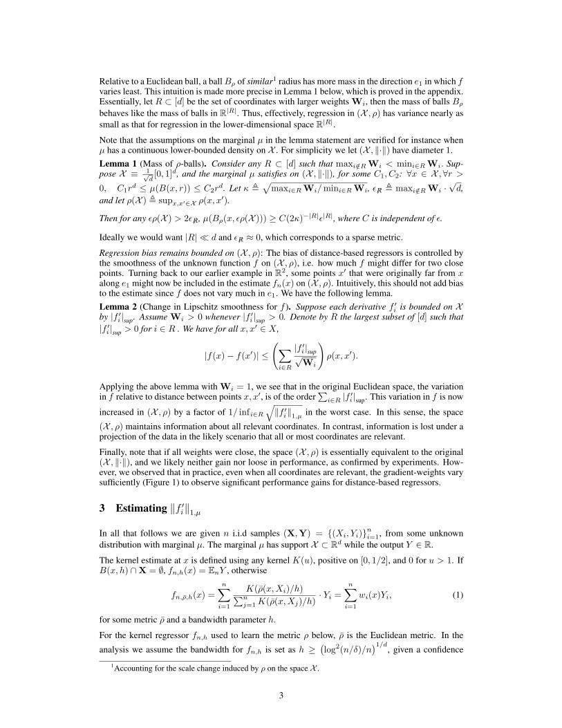
(a) SARCOS robot, joint 7. (b) Parkinson’s. (c) Telecom.

Figure 1: Typical gradient weights{Wi ≈ ‖f ′i‖1,µ

}i∈[d]

for some real-world datasets.

unknown norm ‖f ′i‖1,µ. Moreover we prove finite sample convergence bounds to help guide thepractical tuning of the two parameters t and h.

Most related work

As we mentioned above, metric learning is closest in spirit to the gradient-weighting approach pre-sented here, but our approach is different from metric learning in that we do not search a spaceof possible metrics, but rather estimate a single metric based on gradients. This is far more time-efficient and can be implemented in online applications which require fast preprocessing.

There exists many metric learning approaches, mostly for classification and few for regression (e.g.[1, 2]). The approaches of [1, 2] for regression are meant for batch learning. Moreover [1] is limitedto Gaussian-kernel regression, and [2] is tuned to the particular problem of age estimation. For theproblem of classification, the metric-learning approaches of [3, 4] are meant for online applications,but cannot be used in regression.

In the case of kernel regression and local polynomial regression, multiple bandwidths can be used,one for each coordinate [6]. However, tuning d bandwidth parameters requires searching a d×d grid,which is impractical even in batch mode. The method of [6] alleviates this problem, however onlyin the particular case of local linear regression. Our method applies to any distance-based regressor.

Finally, the ideas presented here are related to recent notions of nonparametric sparsity where it isassumed that the target function is well approximated by a sparse function, i.e. one which varieslittle in most coordinates (e.g. [6], [7]). Here we do not need sparsity, instead we only need thetarget function to vary in some coordinates more than in others. Our approach therefore works evenin cases where the target function is far from sparse.

2 Technical motivation

In this section, we motivate the approach by considering the ideal situation where Wi = ‖f ′i‖1,µ.Let’s consider regression on (X , ρ), where the input space X ⊂ Rd is connected. The predictionperformance of a distance-based estimator (e.g. kernel or k-NN) is well known to be the sum of itsvariance and its bias [8]. Regression on (X , ρ) decreases variance while keeping the bias controlled.

Regression variance decreases on (X , ρ): The variance of a distance based estimate fn(x) is in-versely proportional to the number of samples (and hence the mass) in a neighborhood of x (seee.g. [9]). Let’s therefore compare the masses of ρ-balls and Euclidean balls. Suppose some weightslargely dominate others, for instance in R2, let ‖f ′2‖1,µ � ‖f ′1‖1,µ. A ball Bρ in (X , ρ) then takesthe ellipsoidal shape below which we contrast with the dotted Euclidean ball inside.

2

Relative to a Euclidean ball, a ballBρ of similar1 radius has more mass in the direction e1 in which fvaries least. This intuition is made more precise in Lemma 1 below, which is proved in the appendix.Essentially, let R ⊂ [d] be the set of coordinates with larger weights Wi, then the mass of balls Bρ

behaves like the mass of balls in R|R|. Thus, effectively, regression in (X , ρ) has variance nearly assmall as that for regression in the lower-dimensional space R|R|.

Note that the assumptions on the marginal µ in the lemma statement are verified for instance whenµ has a continuous lower-bounded density on X . For simplicity we let (X , ‖·‖) have diameter 1.Lemma 1 (Mass of ρ-balls). Consider any R ⊂ [d] such that maxi/∈R Wi < mini∈R Wi. Sup-pose X ≡ 1√

d[0, 1]d, and the marginal µ satisfies on (X , ‖·‖), for some C1, C2: ∀x ∈ X ,∀r >

0, C1rd ≤ µ(B(x, r)) ≤ C2r

d. Let κ ,√maxi∈R Wi/mini∈R Wi, ε 6R , maxi/∈R Wi ·

√d,

and let ρ(X ) , supx,x′∈X ρ(x, x′).

Then for any ερ(X ) > 2ε 6R, µ(Bρ(x, ερ(X ))) ≥ C(2κ)−|R|ε|R|, where C is independent of ε.

Ideally we would want |R| � d and ε6R ≈ 0, which corresponds to a sparse metric.

Regression bias remains bounded on (X , ρ): The bias of distance-based regressors is controlled bythe smoothness of the unknown function f on (X , ρ), i.e. how much f might differ for two closepoints. Turning back to our earlier example in R2, some points x′ that were originally far from xalong e1 might now be included in the estimate fn(x) on (X , ρ). Intuitively, this should not add biasto the estimate since f does not vary much in e1. We have the following lemma.Lemma 2 (Change in Lipschitz smoothness for f ). Suppose each derivative f ′i is bounded on Xby |f ′i |sup. Assume Wi > 0 whenever |f ′i |sup > 0. Denote by R the largest subset of [d] such that|f ′i |sup > 0 for i ∈ R . We have for all x, x′ ∈ X ,

|f(x)− f(x′)| ≤

(∑i∈R

|f ′i |sup√Wi

)ρ(x, x′).

Applying the above lemma with Wi = 1, we see that in the original Euclidean space, the variationin f relative to distance between points x, x′, is of the order

∑i∈R |f ′i |sup. This variation in f is now

increased in (X , ρ) by a factor of 1/ infi∈R

√‖f ′i‖1,µ in the worst case. In this sense, the space

(X , ρ) maintains information about all relevant coordinates. In contrast, information is lost under aprojection of the data in the likely scenario that all or most coordinates are relevant.

Finally, note that if all weights were close, the space (X , ρ) is essentially equivalent to the original(X , ‖·‖), and we likely neither gain nor loose in performance, as confirmed by experiments. How-ever, we observed that in practice, even when all coordinates are relevant, the gradient-weights varysufficiently (Figure 1) to observe significant performance gains for distance-based regressors.

3 Estimating ‖f ′i‖1,µ

In all that follows we are given n i.i.d samples (X,Y) = {(Xi, Yi)}ni=1, from some unknowndistribution with marginal µ. The marginal µ has support X ⊂ Rd while the output Y ∈ R.

The kernel estimate at x is defined using any kernel K(u), positive on [0, 1/2], and 0 for u > 1. IfB(x, h) ∩X = ∅, fn,h(x) = EnY , otherwise

fn,ρ,h(x) =n∑

i=1

K(ρ(x,Xi)/h)∑nj=1K(ρ(x,Xj)/h)

· Yi =n∑

i=1

wi(x)Yi, (1)

for some metric ρ and a bandwidth parameter h.

For the kernel regressor fn,h used to learn the metric ρ below, ρ is the Euclidean metric. In the

analysis we assume the bandwidth for fn,h is set as h ≥(log2(n/δ)/n

)1/d, given a confidence

1Accounting for the scale change induced by ρ on the space X .

3

parameter 0 < δ < 1. In practice we would learn h by cross-validation, but for the analysis we onlyneed to know the existence of a good setting of h.

The metric is defined as

Wi , En|fn,h(X + tei)− fn,h(X − tei)|

2t· 1{An,i(X)} = En

[∆t,ifn,h(X) · 1{An,i(X)}

], (2)

where An,i(X) is the event that enough samples contribute to the estimate ∆t,ifn,h(X). For theconsistency result, we assume the following setting:

An,i(X) ≡ mins∈{−t,t}

µn(B(X + sei, h/2)) ≥ αn where αn , 2d ln 2n+ ln(4/δ)

n.

4 Consistency of the estimator Wi of ‖f ′i‖1,µ

4.1 Theoretical setup

4.1.1 Marginal µ

Without loss of generality we assume X has bounded diameter 1. The marginal is assumed to havea continuous density on X and has mass everywhere on X : ∀x ∈ X ,∀h > 0, µ(B(x, h)) ≥ Cµh

d.This is for instance the case if µ has a lower-bounded density on X . Under this assumption, forsamples X in dense regions, X ± tei is also likely to be in a dense region.

4.1.2 Regression function and noise

The output Y ∈ R is given as Y = f(X) + η(X), where Eη(X) = 0. We assume the followinggeneral noise model: ∀δ > 0 there exists c > 0 such that supx∈X PY |X=x (|η(x)| > c) ≤ δ.

We denote by CY (δ) the infimum over all such c. For instance, suppose η(X) has exponentiallydecreasing tail, then ∀δ > 0, CY (δ) ≤ O(ln 1/δ). A last assumption on the noise is that thevariance of (Y |X = x) is upper-bounded by a constant σ2

Y uniformly over all x ∈ X .

Define the τ -envelope of X as X+B(0, τ) , {z ∈ B(x, τ), x ∈ X}. We assume there exists τ suchthat f is continuously differentiable on the τ -envelope X + B(0, τ). Furthermore, each derivativef ′i(x) = e>i ∇f(x) is upper bounded on X + B(0, τ) by |f ′i |sup and is uniformly continuous onX +B(0, τ) (this is automatically the case if the support X is compact).

4.1.3 Parameters varying with t

Our consistency results are expressed in terms of the following distributional quantities. For i ∈ [d],define the (t, i)-boundary of X as ∂t,i(X ) , {x : {x+ tei, x− tei} * X}. The smaller the massµ(∂t,i(X )) at the boundary, the better we approximate ‖f ′i‖1,µ.

The second type of quantity is εt,i , supx∈X , s∈[−t,t] |f ′i(x)− f ′i(x+ sei)|.

Since µ has continuous density on X and ∇f is uniformly continuous on X +B(0, τ), we automat-ically have µ(∂t,i(X ))

t→0−−−→ 0 and εt,it→0−−−→ 0.

4.2 Main theorem

Our main theorem bounds the error in estimating each norm ‖f ′i‖1,µ with Wi. The main technicalhurdles are in handling the various sample inter-dependencies introduced by both the estimatesfn,h(X) and the events An,i(X), and in analyzing the estimates at the boundary of X .Theorem 1. Let t + h ≤ τ , and let 0 < δ < 1. There exist C = C(µ,K(·)) and N = N(µ) suchthat the following holds with probability at least 1− 2δ. Define A(n) , Cd · log(n/δ) ·C2

Y (δ/2n) ·σ2Y / log

2(n/δ). Let n ≥ N , we have for all i ∈ [d]:∣∣∣Wi − ‖f ′i‖1,µ∣∣∣ ≤ 1

t

√A(n)

nhd+ h ·

∑i∈[d]

|f ′i |sup

+ 2 |f ′i |sup

(√ln 2d/δ

n+ µ (∂t,i(X ))

)+ εt,i.

4

The bound suggest to set t in the order of h or larger. We need t to be small in order for µ (∂t,i(X ))and εt,i to be small, but t need to be sufficiently large (relative to h) for the estimates fn,h(X + tei)and fn,h(X − tei) to differ sufficiently so as to capture the variation in f along ei.

The theorem immediately implies consistency for t n→∞−−−−→ 0, h n→∞−−−−→ 0, h/t n→∞−−−−→ 0, and(n/ logn)hdt2

n→∞−−−−→ ∞. This is satisfied for many settings, for example t ∝√h and h ∝ 1/ log n.

4.3 Proof of Theorem 1

The main difficulty in bounding∣∣∣Wi − ‖f ′i‖1,µ

∣∣∣ is in circumventing certain depencies: both quanti-ties fn,h(X) andAn,i(X) depend not just onX ∈ X, but on other samples in X, and thus introduceinter-dependencies between the estimates ∆t,ifn,h(X) for different X ∈ X.

To handle these dependencies, we carefully decompose∣∣∣Wi − ‖f ′i‖1,µ

∣∣∣, i ∈ [d], starting with:∣∣∣Wi − ‖f ′i‖1,µ∣∣∣ ≤ |Wi − En |f ′i(X)||+

∣∣∣En |f ′i(X)| − ‖f ′i‖1,µ∣∣∣ . (3)

The following simple lemma bounds the second term of (3).

Lemma 3. With probability at least 1− δ, we have for all i ∈ [d],∣∣∣En |f ′i(X)| − ‖f ′i‖1,µ∣∣∣ ≤ |f ′i |sup ·

√ln 2d/δ

n.

Proof. Apply a Chernoff bound, and a union bound on i ∈ [d].

Now the first term of equation (3) can be further bounded as

|Wi − En |f ′i(X)|| ≤∣∣Wi − En |f ′i(X)| · 1{An,i(X)}

∣∣+ En |f ′i(X)| · 1{An,i(X)}≤∣∣Wi − En |f ′i(X)| · 1{An,i(X)}

∣∣+ |f ′i |sup · En1{An,i(X)}. (4)

We will bound each term of (4) separately.

The next lemma bounds the second term of (4). It is proved in the appendix. The main technicalityin this lemma is that, for any X in the sample X, the event An,i(X) depends on other samples in X.

Lemma 4. Let ∂t,i(X ) be defined as in Section (4.1.3). For n ≥ n(µ), with probability at least1− 2δ, we have for all i ∈ [d],

En1{An,i(X)} ≤√

ln 2d/δ

n+ µ (∂t,i(X )) .

It remains to bound∣∣Wi − En |f ′i(X)| · 1{An,i(X)}

∣∣. To this end we need to bring in f through thefollowing quantities:

Wi , En

[|f(X + tei)− f(X − tei)|

2t· 1{An,i(X)}

]= En

[∆t,if(X) · 1{An,i(X)}

]and for any x ∈ X , define fn,h(x) , EY|Xfn,h(x) =

∑i wi(x)f(xi).

The quantity Wi is easily related to En |f ′i(X)| · 1{An,i(X)}. This is done in Lemma 5 below. Thequantity fn,h(x) is needed when relating Wi to Wi.

Lemma 5. Define εt,i as in Section (4.1.3). With probability at least 1− δ, we have for all i ∈ [d],∣∣∣Wi − En |f ′i(X)| · 1{An,i(X)}

∣∣∣ ≤ εt,i.

5

Proof. We have f(x+ tei)− f(x− tei) =∫ t

−tf ′i(x+ sei) ds and therefore

2t (f ′i(x)− εt,i) ≤ f(x+ tei)− f(x− tei) ≤ 2t (f ′i(x) + εt,i) .

It follows that∣∣ 12t |f(x+ tei)− f(x− tei)| − |f ′i(x)|

∣∣ ≤ εt,i, therefore∣∣∣Wi − En |f ′i(X)| · 1{An,i(X)}

∣∣∣ ≤ En

∣∣∣∣ 12t |f(x+ tei)− f(x− tei)| − |f ′i(x)|∣∣∣∣ ≤ εt,i.

It remains to relate Wi to Wi. We have

2t∣∣∣Wi − Wi

∣∣∣ =2t∣∣En(∆t,ifn,h(X)−∆t,if(X)) · 1{An,i(X)}

∣∣≤2 max

s∈{−t,t}En|fn,h(X + sei)− f(X + sei)| · 1{An,i(X)}

≤2 maxs∈{−t,t}

En

∣∣∣fn,h(X + sei)− fn,h(X + sei)∣∣∣ · 1{An,i(X)} (5)

+ 2 maxs∈{−t,t}

En

∣∣∣fn,h(X + sei)− f(X + sei)∣∣∣ · 1{An,i(X)}. (6)

We first handle the bias term (6) in the next lemma which is given in the appendix.

Lemma 6 (Bias). Let t+ h ≤ τ . We have for all i ∈ [d], and all s ∈ {t,−t}:

En

∣∣∣fn,h(X + sei)− f(X + sei)∣∣∣ · 1{An,i(X)} ≤ h ·

∑i∈[d]

|f ′i |sup .

The variance term in (5) is handled in the lemma below. The proof is given in the appendix.

Lemma 7 (Variance terms). There exist C = C(µ,K(·)) such that, with probability at least 1− 2δ,we have for all i ∈ [d], and all s ∈ {−t, t}:

En

∣∣∣fn,h(X + sei)− fn,h(X + sei)∣∣∣ · 1{An,i(X)} ≤

√Cd · log(n/δ)C2

Y (δ/2n) · σ2Y

n(h/2)d.

The next lemma summarizes the above results:

Lemma 8. Let t + h ≤ τ and let 0 < δ < 1. There exist C = C(µ,K(·)) such that the followingholds with probability at least 1− 2δ. Define A(n) , Cd · log(n/δ) · C2

Y (δ/2n) · σ2Y / log

2(n/δ).We have

∣∣Wi − En |f ′i(X)| · 1{An,i(X)}∣∣ ≤1

t

√A(n)

nhd+ h ·

∑i∈[d]

|f ′i |sup

+ εt,i.

Proof. Apply lemmas 5, 6 and 7, in combination with equations 5 and 6.

To complete the proof of Theorem 1, apply lemmas 8 and 3 in combination with equations 3 and 4.

5 Experiments

5.1 Data description

We present experiments on several real-world regression datasets. The first two datasets describe thedynamics of 7 degrees of freedom of robotic arms, Barrett WAM and SARCOS [10, 11]. The inputpoints are 21-dimensional and correspond to samples of the positions, velocities, and accelerationsof the 7 joints. The output points correspond to the torque of each joint. The far joints (1, 5, 7)

6

Barrett joint 1 Barrett joint 5 SARCOS joint 1 SARCOS joint 5 HousingKR error 0.50 ± 0.02 0.50 ± 0.03 0.16 ± 0.02 0.14 ± 0.02 0.37 ±0.08KR-ρ error 0.38± 0.03 0.35 ± 0.02 0.14 ± 0.02 0.12 ± 0.01 0.25 ±0.06KR time 0.39 ± 0.02 0.37 ± 0.01 0.28 ± 0.05 0.23 ± 0.03 0.10 ±0.01KR-ρ time 0.41 ± 0.03 0.38 ± 0.02 0.32 ± 0.05 0.23 ± 0.02 0.11 ±0.01

Concrete Strength Wine Quality Telecom Ailerons Parkinson’sKR error 0.42 ± 0.05 0.75 ± 0.03 0.30±0.02 0.40±0.02 0.38±0.03KR-ρ error 0.37 ± 0.03 0.75 ± 0.02 0.23±0.02 0.39±0.02 0.34±0.03KR time 0.14 ± 0.02 0.19 ± 0.02 0.15±0.01 0.20±0.01 0.30±0.03KR-ρ time 0.14 ± 0.01 0.19 ± 0.02 0.16±0.01 0.21±0.01 0.30±0.03

Barrett joint 1 Barrett joint 5 SARCOS joint 1 SARCOS joint 5 Housingk-NN error 0.41 ± 0.02 0.40 ± 0.02 0.08 ± 0.01 0.08 ± 0.01 0.28 ±0.09k-NN-ρ error 0.29 ± 0.01 0.30 ± 0.02 0.07 ± 0.01 0.07 ± 0.01 0.22±0.06k-NN time 0.21 ± 0.04 0.16 ± 0.03 0.13 ± 0.01 0.13 ± 0.01 0.08 ±0.01k-NN-ρ time 0.13 ± 0.04 0.16 ± 0.03 0.14 ± 0.01 0.13 ± 0.01 0.08 ±0.01

Concrete Strength Wine Quality Telecom Ailerons Parkinson’sk-NN error 0.40 ± 0.04 0.73 ± 0.04 0.13±0.02 0.37±0.01 0.22±0.01k-NN-ρ error 0.38 ± 0.03 0.72 ± 0.03 0.17±0.02 0.34±0.01 0.20±0.01k-NN time 0.10 ± 0.01 0.15 ± 0.01 0.16±0.02 0.12±0.01 0.14±0.01k-NN-ρ time 0.11 ± 0.01 0.15 ± 0.01 0.15±0.01 0.11±0.01 0.15±0.01

Table 1: Normalized mean square prediction errors and average prediction time per point (in mil-liseconds). The top two tables are for KR vs KR-ρ and the bottom two for k-NN vs k-NN-ρ.

1000 2000 3000 4000 50000

0.02

0.04

0.06

0.08

0.1

number of training points

erro

r

KR errorKR−ρ error

(a) SARCOS, joint 7, with KR

1000 2000 3000 4000 50000.32

0.34

0.36

0.38

0.4

0.42

0.44

number of training points

erro

r

KR errorKR−ρ error

(b) Ailerons with KR

1000 2000 3000 4000 5000 6000 70000.1

0.15

0.2

0.25

0.3

0.35

number of training points

erro

r

KR errorKR−ρ error

(c) Telecom with KR

1000 2000 3000 4000 50000.005

0.01

0.015

0.02

0.025

number of training points

erro

r

k−NN errork−NN−ρ error

(d) SARCOS, joint 7, with k-NN

1000 2000 3000 4000 5000

0.29

0.3

0.31

0.32

0.33

0.34

0.35

0.36

0.37

0.38

number of training points

erro

r

k−NN errork−NN−ρ error

(e) Ailerons with k-NN

1000 2000 3000 4000 5000 6000 70000

0.05

0.1

0.15

0.2

number of training points

erro

r

k−NN errork−NN−ρ error

(f) Telecom with k-NN

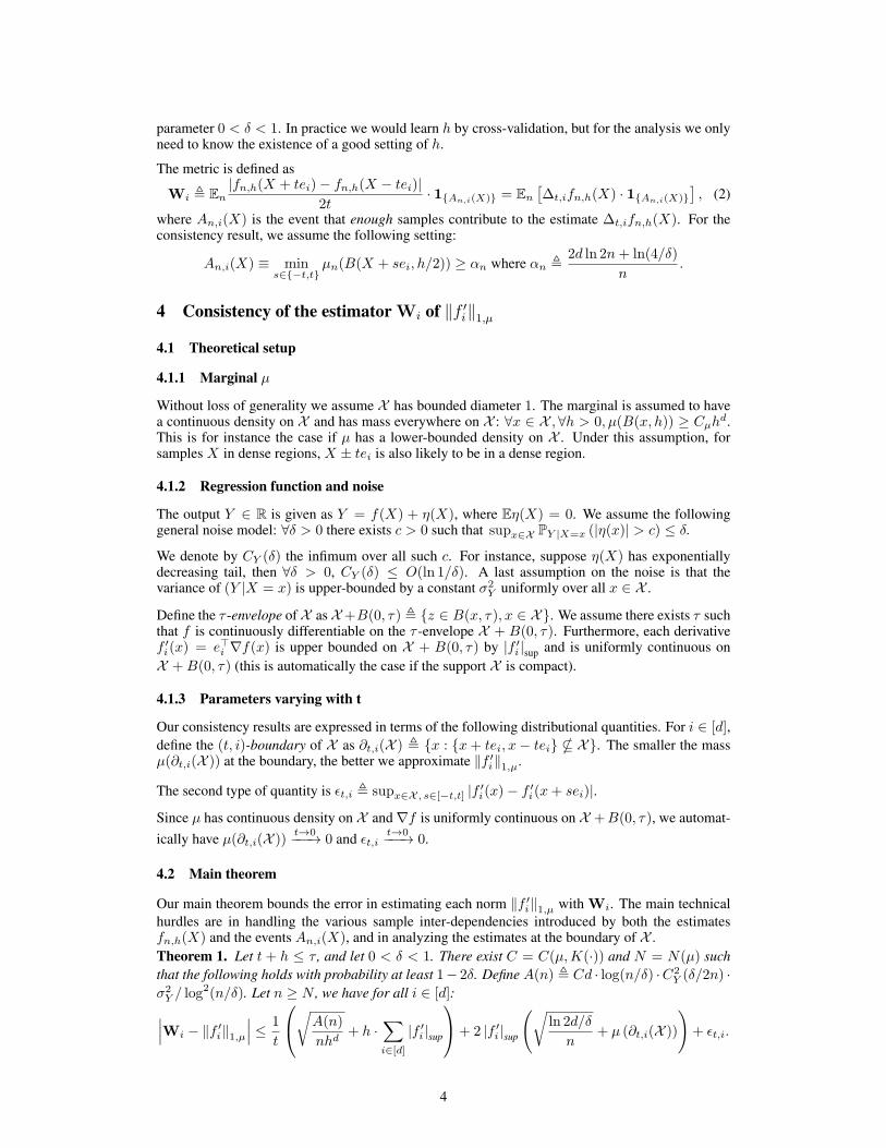
Figure 2: Normalized mean square prediction error over 2000 points for varying training sizes.Results are shown for k-NN and kernel regression (KR), with and without the metric ρ.

correspond to different regression problems and are the only results reported. Expectedly, results forthe other joints are similarly good.

The other datasets are taken from the UCI repository [12] and from [13]. The concrete strengthdataset (Concrete Strength) contains 8-dimensional input points, describing age and ingredients ofconcrete, the output points are the compressive strength. The wine quality dataset (Wine Quality)contains 11-dimensional input points corresponding to the physicochemistry of wine samples, theoutput points are the wine quality. The ailerons dataset (Ailerons) is taken from the problem of flyinga F16 aircraft. The 5-dimensional input points describe the status of the aeroplane, while the goal is

7

to predict the control action on the ailerons of the aircraft. The housing dataset (Housing) concernsthe task of predicting housing values in areas of Boston, the input points are 13-dimensional. TheParkinson’s Telemonitoring dataset (Parkison’s) is used to predict the clinician’s Parkinson’s diseasesymptom score using biomedical voice measurements represented by 21-dimensional input points.We also consider a telecommunication problem (Telecom), wherein the 47-dimensional input pointsand the output points describe the bandwidth usage in a network.

For all datasets we normalize each coordinate with its standard deviation from the training data.

5.2 Experimental setup

To learn the metric, we set h by cross-validation on half the training points, and we set t = h/2for all datasets. Note that in practice we might want to also tune t in the range of h for evenbetter performance than reported here. The event An,i(X) is set to reject the gradient estimate∆n,ifn,h(X) at X if no sample contributed to one the estimates fn,h(X ± tei).

In each experiment, we compare kernel regression in the euclidean metric space (KR) and in thelearned metric space (KR-ρ), where we use a box kernel for both. Similar comparisons are madeusing k-NN and k-NN-ρ. All methods are implemented using a fast neighborhood search procedure,namely the cover-tree of [14], and we also report the average prediction times so as to confirm that,on average, time-performance is not affected by using the metric.

The parameter k in k-NN/k-NN-ρ, and the bandwidth in KR/KR-ρ are learned by cross-validationon half of the training points. We try the same range of k (from 1 to 5 log n) for both k-NN andk-NN-ρ. We try the same range of bandwidth/space-diameter (a grid of size 0.02 from 1 to 0.02 )for both KR and KR-ρ: this is done efficiently by starting with a log search to detect a smaller range,followed by a grid search on a smaller range.

Table 5 shows the normalized Mean Square Errors (nMSE) where the MSE on the test set is normal-ized by variance of the test output. We use 1000 training points in the robotic datasets, 2000 trainingpoints in the Telecom, Parkinson’s, Wine Quality, and Ailerons datasets, and 730 training points inConcrete Strength, and 300 in Housing. We used 2000 test points in all of the problems, except forConcrete, 300 points, and Housing, 200 points. Averages over 10 random experiments are reported.

For the larger datasets (SARCOS, Ailerons, Telecom) we also report the behavior of the algorithms,with and without metric, as the training size n increases (Figure 2).

5.3 Discussion of results

From the results in Table 5 we see that virtually on all datasets the metric helps improve the perfor-mance of the distance based-regressor even though we did not tune t to the particular problem (re-member t = h/2 for all experiments). The only exceptions are for Wine Quality where the learnedweights are nearly uniform, and for Telecom with k-NN. We noticed that the Telecom dataset hasa lot of outliers and this probably explains the discrepancy, besides from the fact that we did notattempt to tune t. Also notice that the error of k-NN is already low for small sample sizes, makingit harder to outperform. However, as shown in Figure 2, for larger training sizes k-NN-ρ gains onk-NN. The rest of the results in Figure 2 where we vary n are self-descriptive: gradient weightingclearly improves the performance of the distance-based regressors.

We also report the average prediction times in Table 5. We see that running the distance-basedmethods with gradient weights does not affect estimation time. Last, remember that the metric canbe learned online at the cost of only 2d times the average kernel estimation time reported.

6 Final remarks

Gradient weighting is simple to implement, computationally efficient in batch-mode and online, andmost importantly improves the performance of distance-based regressors on real-world applications.In our experiments, most or all coordinates of the data are relevant, yet some coordinates are moreimportant than others. This is sufficient for gradient weighting to yield gains in performance. Webelieve there is yet room for improvement given the simplicity of our current method.

8

References[1] Kilian Q. Weinberger and Gerald Tesauro. Metric learning for kernel regression. Journal of

Machine Learning Research - Proceedings Track, 2:612–619, 2007.[2] Bo Xiao, Xiaokang Yang, Yi Xu, and Hongyuan Zha. Learning distance metric for regression

by semidefinite programming with application to human age estimation. In Proceedings of the17th ACM international conference on Multimedia, pages 451–460, 2009.

[3] Shai Shalev-shwartz, Yoram Singer, and Andrew Y. Ng. Online and batch learning of pseudo-metrics. In ICML, pages 743–750. ACM Press, 2004.

[4] Jason V. Davis, Brian Kulis, Prateek Jain, Suvrit Sra, and Inderjit S. Dhillon. Information-theoretic metric learning. In ICML, pages 209–216, 2007.

[5] W. Hardle and T. Gasser. On robust kernel estimation of derivatives of regression functions.Scandinavian journal of statistics, pages 233–240, 1985.

[6] J. Lafferty and L. Wasserman. Rodeo: Sparse nonparametric regression in high dimensions.Arxiv preprint math/0506342, 2005.

[7] L. Rosasco, S. Villa, S. Mosci, M. Santoro, and A. Verri. Nonparametric sparsity and regular-ization. http://arxiv.org/abs/1208.2572, 2012.

[8] L. Gyorfi, M. Kohler, A. Krzyzak, and H. Walk. A Distribution Free Theory of NonparametricRegression. Springer, New York, NY, 2002.

[9] S. Kpotufe. k-NN Regression Adapts to Local Intrinsic Dimension. NIPS, 2011.[10] Duy Nguyen-Tuong, Matthias W. Seeger, and Jan Peters. Model learning with local gaussian

process regression. Advanced Robotics, 23(15):2015–2034, 2009.[11] Duy Nguyen-Tuong and Jan Peters. Incremental online sparsification for model learning in

real-time robot control. Neurocomputing, 74(11):1859–1867, 2011.[12] A. Frank and A. Asuncion. UCI machine learning repository. http://archive.ics.

uci.edu/ml. University of California, Irvine, School of Information and Computer Sci-ences, 2012.

[13] Luis Torgo. Regression datasets. http://www.liaad.up.pt/˜ltorgo. University ofPorto, Department of Computer Science, 2012.

[14] A. Beygelzimer, S. Kakade, and J. Langford. Cover trees for nearest neighbors. ICML, 2006.[15] V. Vapnik and A. Chervonenkis. On the uniform convergence of relative frequencies of events

to their expectation. Theory of probability and its applications, 16:264–280, 1971.

9

Appendix

A Consistency lemmas

We need the following VC result.Lemma 9 (Relative VC bounds [15]). Let 0 < δ < 1 and define αn = (2d ln 2n+ ln(4/δ)) /n.

Then with probability at least 1− δ over the choice of X, all balls B ∈ Rd satisfy

µ(B) ≤ µn(B) +√µn(B)αn + αn.

Proof of Lemma 4. Let Ai(X) denote the event that mins∈{−t,t} µ(B(X + sei, h/2)) < 3αn. ByLemma 9, with probability at least 1− δ, ∀i ∈ [d], An,i(X) =⇒ Ai(X) so that En1{An,i(X)} ≤En1{Ai(X)}.

Using a Chernoff bound, followed by a union bound on [d], we also have with probability at least1− δ that En1{Ai(X)} ≤ E1{Ai(X)} +

√ln(2d/δ)/n.

Finally, E1{Ai(X)} ≤ E[1{Ai(X)}|X ∈ X \ ∂t,i(X )

]+ µ (∂t,i(X )). The first term is 0 for large

n. This is true since, for x ∈ X \∂t,i(X ), for all i ∈ [d] and s ∈ {−t, t}, x+sei ∈ X , and thereforeµ(B(x+ sei, h/2)) ≥ Cµ(h/2)

d ≥ 3αn for our setting of h (see Section 3).

Proof of Lemma 6. Let x = X + sei. For any Xi ∈ X, let vi denote the unit vector in direction(Xi − x). We have∣∣∣fn,h(x)− f(x)

∣∣∣ ≤∑i

wi(x) |f(Xi)− f(x)| =∑i

wi(x)

∣∣∣∣∣∫ ‖Xi−x‖

0

v>i ∇f(x+ svi) ds

∣∣∣∣∣≤∑i

wi(x) ‖Xi − x‖ · maxx′∈X+B(0,τ)

∥∥v>i ∇f(x′)∥∥ ≤ h ·∑i∈[d]

|f ′i |sup .

Multiply the l.h.s. by 1{An,i(X)}, take the empirical expectation and conclude.

The variance lemma is handled in way similar to an analysis of [9] on k-NN regression. The maintechnicality here is that the number of points contributing to the estimate (and hence the variance) isnot a constant as with k-NN.

Proof of Lemma 7. Assume that An,i(X) is true, and fix x = X + sei. The following variancebound is quickly obtained:

EY|X

∣∣∣fn,h(x)− fn,h(x)∣∣∣2 ≤ σ2

Y ·∑i∈[n]

wi(x) ≤ σ2Y ·max

i∈[n]wi(x).

Let Yx denote the Y values of samples Xi ∈ B(x, h), and write ψ(Yx) ,∣∣∣fn,h(x)− fn,h(x)

∣∣∣.We next relate ψ(Yx) to the above variance.

Let Yδ denote the event that for all Yi ∈ Y, |Yi − f(Xi)| ≤ CY (δ/2n) · σY . By definition ofCY (δ/2n), the event Yδ happens with probability at least 1− δ/2 ≥ 1/2. We therefore have that

PY|X(ψ(Yx) > 2EY|Xψ(Yx) + ε

)≤ PY|X

(ψ(Yx) > EY|X,Yδ

ψ(Yx) + ε)

≤ PY|X,Yδ

(ψ(Yx) > EY|X,Yδ

ψ(Yx) + ε)+ δ/2.

Now, it can be verified that, by McDiarmid’s inequality, we have

PY|X,Yδ

(ψ(Yx) > EY|X,Yδ

ψ(Yx) + ε)≤ exp

−2ε2/C2Y (δ/2n) · σ2

Y

∑i∈[n]

w2i (x)

.

10

Notice that the number of possible sets Yx (over x ∈ X ) is at most the n-shattering number of ballsin Rd. By Sauer’s lemma we know this number is bounded by (2n)d+2. We therefore have by aunion bound that, with probability at least 1− δ, for all x ∈ X satisfying B(x, h/2) ∩X 6= ∅,

ψ(Yx) ≤ 2EY|Xψ(Yx) +

√(d+ 2) · log(n/δ)C2

Y (δ/2n) · σ2Y

∑i∈[n]

w2i (x)

≤ 2(EY|Xψ

2(Yx))1/2

+√(d+ 2) · log(n/δ)C2

Y (δ/2n) · σ2Y ·max

iwi(x)

≤√Cd · log(n/δ)C2

Y (δ/2n) · σ2Y /nµn((B(x, h/2)),

where the second inequality is obtained by applying Jensen’s, and the last inequality is due to thefact that the kernel weights are upper and lower-bounded on B(x, h/2).

Now by Lemma 9, with probability at least 1 − δ, for all X such that An,i(X) is true, we havefor all s ∈ {−t, t}, 3µn((B(x, h/2)) ≥ µ((B(x, h/2)) ≥ Cµ(h/2)

d. Integrate this into the aboveinequality, take the empirical expectation and conclude.

B Properties of the metric space (X , ρ)

The following definitions are reused throughout the section. For any R ⊂ [d], define κ ,√maxi∈R Wi/mini∈R Wi, and let ε6R , maxi/∈R Wi.

The next lemma is preliminary to establishing the mass of balls on (X , ρ) in Lemma 1.

Lemma 10. Suppose X ≡ 1√d[0, 1]d, and µ satisfies on (X , ‖·‖), for some C1, C2: ∀x ∈ X ,∀r >

0, C1rd ≤ µ(B(x, r)) ≤ C2r

d. Note that this condition is satisfied for instance if µ has acontinuous lower-bounded density on X .

The above condition implies a sufficient condition for Lemma 1. That is, for any R ⊂ [d], andpseudo-metric ‖x− x′‖R ,

√∑i∈R(x

i − x′i)2, µ has the following doubling property over ballsBR in the pseudo-metric space (X , ‖·‖R) for some constant C:

∀x ∈ X ,∀r > 0,∀ε > 0, µ(BR(x, r)) ≤ Cε−|R| · µ(BR(x, εr)).

Proof. Fix x ∈ X and r > 0. It can be verified that BR(x, r) can be covered by Cr−(d−|R|)

Euclidean balls of radius r, for some C independent of r. Let B(z, r) denote the ball with thelargest mass in the cover. We then have by a union bound

µ(BR(x, r)) ≤ Cr−(d−|R|)µ(B(z, r)) ≤ Cr−(d−|R|) · C2rd ≤ C · C2r

|R|.

Similarly, for some C independent of r,BR(x, r) can be packed with Cr−(d−|R|) disjoint Euclideanballs of radius r. Let B(z, r) denote the ball with the smallest mass in the packing. We have

µ(BR(x, r)) ≥ Cr−(d−|R|)µ(B(z, r)) ≥ Cr−(d−|R|) · C1rd ≥ C · C1r

|R|.

Since the above holds for any r > 0, including εr for any ε > 0, the conclusion is immediate.

Proof of Lemma 1. First apply Lemma 10. Notice that the doubling property of µ on (X , ‖·‖R)similarly implies for balls BρR

in (X , ρR) that ∀x ∈ X ,∀r > 0,∀ε > 0, µ(BρR(x, r)) ≤ Cε−|R| ·

µ(BρR(x, εr)).

For any x, x′ ∈ X one can check that ρ(x, x′) ≤ κρR(x, x′) + ε6R ≤ κρR(x, x

′) + ερ(X )/2. Itfollows that for any x ∈ X , Bρ(x, ερ(X )) ⊃ BρR(x, ερ(X )/2κ). Now since ρR(x, x′) ≤ ρ(x, x′),the ρR-diameter of X is at most ρ(X ), and we have

µ(Bρ(x, ερ(X ))) ≥ µ(BρR(x, ερ(X )/2κ) ≥ C(ε/2κ)|R|.

11

Proof of Lemma 2. Let x 6= x′ and v = (x − x′)/ ‖x− x′‖. Clearly vi ≤ ρ(x, x′)/(‖x− x′‖ ·√Wi). We have

|f(x)− f(x′)| ≤∫ ‖x−x′‖

0

∣∣v>∇f(x+ sv)∣∣ ds ≤ ∫ ‖x−x′‖

0

∑i∈R

∣∣vi · f ′i(x+ sv)∣∣ ds

≤∑i∈R

∫ ‖x−x′‖

0

∣∣vi∣∣ · |f ′i |sup ≤∑i∈R

ρ(x, x′)√Wi

|f ′i |sup .

12