Gradient Evaluation on a Quadtree Based Finite Volume Grid · Gradient Evaluation on a Quadtree Based Finite Volume Grid Kriv a Zuzana, Handlovi´ cov ´a Angela and Mikula Karol

Gradient Evaluation on a Quadtree Based FiniteVolume Grid

Kriva Zuzana, Handlovicova Angela and Mikula Karol

Abstract Many problems described by nonlinear PDEs need good approximationsof gradients on finite volumes. Using finite volume methods, this can be difficulttask if discretization of a computational domain does not fulfill the classical or-thogonality property. Such a situation can occur, e.g., during coarsening in imageprocessing using quadtree grids. We present a construction of an adjusted quadtreegrid for which the connection of representative points of two adjacent finite vol-umes is perpendicular to their common boundary. On the other hand, for such anadjusted grid, the intersection of representative points connection with a finite vol-ume boundary is not a middle point of their common edge. In this paper we presenta new method of gradient evaluation for such a situation.

1 The computational grid

In this section we introduce our finite volume computational grid, its constructionand its properties. Our purpose is to build the grid using large elements for regionswith homogeneous values of a solution function - in our experiment representingimage intensities. To this purpose we first build a graded quadtree, i.e. the quadtree,in which the difference in a level between adjacent cells is constrained, in our case toone. Grids associated with such trees are often used in order to produce proceduresthat are easier to implement. Moreover, in our case it is an inevitable requirement tobe able to adjust the quadtree to the consistent finite volume grid. The consistent gridpossesses the important property that the connection of two representative points oftwo adjacent finite volumes is perpendicular to their common boundary, which is

Kriva Zuzana, Handlovicova Angela and Mikula KarolDepartment of Mathematics, Slovak University of Technology in Bratislava, Faculty of CivilEngineering, Radlinskeho 11, 813 68 Bratislava, Slovak Republic, e-mail: [email protected], [email protected], [email protected]

1

FVCA7, 100, v1 (major): ’Gradient Evalua...’ 1

2 Kriva Zuzana, Handlovicova Angela and Mikula Karol

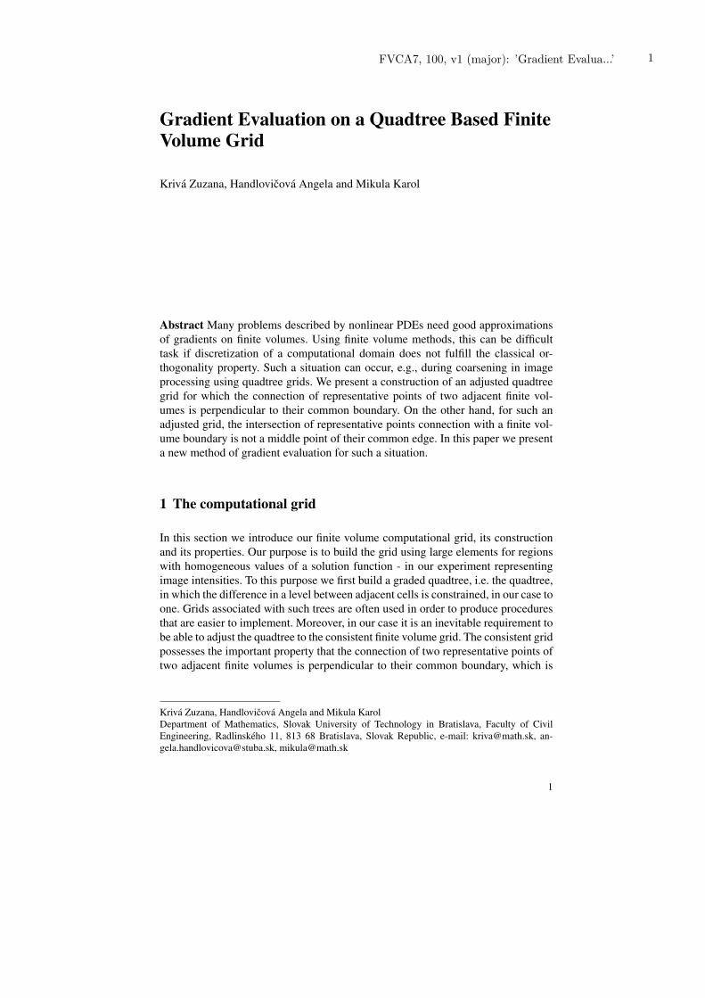
Fig. 1 An example of the original quadtree grid together with the representative points of its ele-ments (on the left). This grid is transformed into the consistent one (on the right).

an important fact when we use the classical finite volume discretization [2]. Anexample of a quadtree and a corresponding consistent grid is displayed in Fig.1.

Building the quadtree. Let us suppose that our data is given on a regular non-adaptive square grid (which corresponds e.g. to the pixel structure of an image).First we build the quadtree by merging the elements with similar values from thesmaller cells to the larger cells, i.e. from leaves to the root. The old values are eitherunchanged, or replaced by averaging the values from the processed area. Duringthis process, the information about successful or unsuccessful merging is stored in abinary field with the size corresponding to the image. Moreover, this information isstored in such a way that it enables us to create a graded quadtree with a prescribedratio of elements. It can be also used as a stopping criterion during traversing thequadtree and to test the configurations of elements - the leaves of the quadtree.

As we have already mentioned, in order to simplify creating the linear systemmatrix, where access to neighbors is needed, and to enable creating the consistentgrid, we require that the ratio of sides of two adjacent squares is 1 : 1, 1 : 2 or 2 : 1.The used technique of building the quadtree adaptive grids is described in [4]. Ituses the following coarsening criterion: the cells are merged if a difference in theirintensities is below a prescribed tolerance ε .

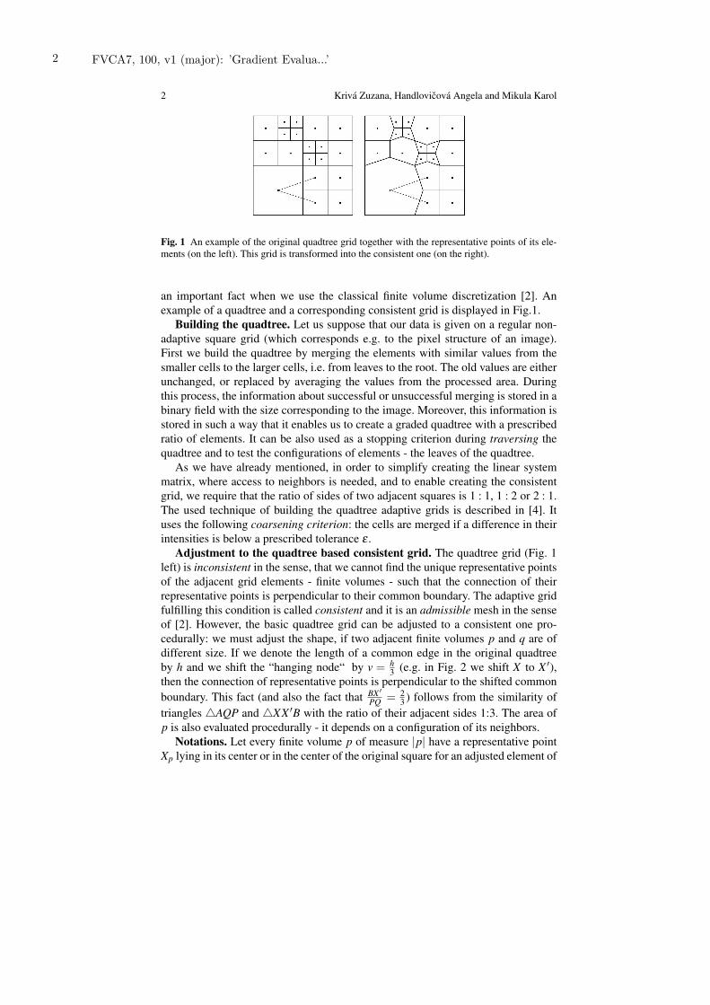
Adjustment to the quadtree based consistent grid. The quadtree grid (Fig. 1left) is inconsistent in the sense, that we cannot find the unique representative pointsof the adjacent grid elements - finite volumes - such that the connection of theirrepresentative points is perpendicular to their common boundary. The adaptive gridfulfilling this condition is called consistent and it is an admissible mesh in the senseof [2]. However, the basic quadtree grid can be adjusted to a consistent one pro-cedurally: we must adjust the shape, if two adjacent finite volumes p and q are ofdifferent size. If we denote the length of a common edge in the original quadtreeby h and we shift the “hanging node“ by v = h

3 (e.g. in Fig. 2 we shift X to X ′),then the connection of representative points is perpendicular to the shifted commonboundary. This fact (and also the fact that BX ′

PQ = 23 ) follows from the similarity of

triangles 4AQP and 4XX ′B with the ratio of their adjacent sides 1:3. The area ofp is also evaluated procedurally - it depends on a configuration of its neighbors.

Notations. Let every finite volume p of measure |p| have a representative pointXp lying in its center or in the center of the original square for an adjusted element of

2 FVCA7, 100, v1 (major): ’Gradient Evalua...’

Gradient Evaluation on a Quadtree Based Finite Volume Grid 3

Fig. 2 Adjustment to the consistent grid. |XX ′| = v = 13 h. XB= 2

3 PA, hence BX ′PQ = 2

3 . Examples ofthe shapes where the intersection of the connection of representative points and a common edge σis not the midpoint of σ .

the consistent grid. The common interface of p and q is a line segment - an edge σpqwith a nonzero measure in IR denoted by |σpq| and dpq = |Xq − Xp| is the distanceof representative points. Let us denote by Xσ auch a point of σpq, which representsthe intersection of the line segment XpXq and σpq. In our consistent grid, XpXq isperpendicular to σ , but the intersection Xσ is not the midpoint of σ in the generalcase. Let us denote by X∗

σ the midpoint of the edge σ . By Ep we denote the set ofall edges σ of p. When we speak about a unit outer normal vector to σ ∈ Ep, wedenote it by npσ .

2 Approximation of the gradient on the consistent grid

Our method for evaluation of gradients on finite volumes is based on [3]. Such amethod works locally in that sense that we consider also representative points onfinite volume edges, but not values at the corners. Then, with a help of these pointswe only need access to neighbors sharing a common edge, which is important whenworking on adaptive grids.

When solving PDEs where nonlinearities depend on the solution gradient, themethod from [3] works as follows:

1. for edges σ of a finite volume p we define representative points X∗σ - their mid-

points, it must hold X∗σ = Xσ ,

2. with a help of these points, we evaluate the norm of gradient on p locally usingthe consequence of the Stokes formula, see (3)-(4),

3. discrete equation for the finite volume p is derived locally,4. values of solution in X∗

σ are obtained by using conservation principle.

FVCA7, 100, v1 (major): ’Gradient Evalua...’ 3

4 Kriva Zuzana, Handlovicova Angela and Mikula Karol

In the consistent adaptive grid X∗σ 6= Xσ in general. Such a situation occurs on edges

containing a hanging node in the original quadtree grid. The most critical shape inthis sense is the sharp element where Xσ is not the midpoint on any of the edges(Fig.2 right).

Let us suppose the linear approximation of the solution over the finite volume p.At X ∈ p any linear function can be written as

u(X) = u(Xp)+∇u · (X −Xp) = up +∇u · (X −Xp). (1)

If X = Xσ it holdsuσ −up = ∇u · (Xσ −Xp), (2)

where uσ , up represent values of the solution at points Xσ and Xp. The gradient ofthe linear function is a constant vector in IR2, thus also over a control volume p. Itwill be denoted by ∇u. Then it holds

∇u =1|p|∫

p

∇udX =1|p|∫

∂ p

unpdS =1|p| ∑

σ∈Ep

∫

σ

(up +∇u · (X −Xp))npσ dS

=1|p|up ∑

σ∈Ep

|σ |npσ +1|p| ∑

σ∈Ep

|σ |∇u · (X∗σ −Xp)npσ . (3)

The term ∑σ∈Ep

|σ |npσ = 0 and the expression |σ |∇u(X∗σ − Xp)npσ represents the

precise integration of a linear function over the edge σ . Thus we have

∇u =1|p| ∑

σ∈Ep

|σ |∇u · (X∗σ −Xp)npσ . (4)

On the edges, where Xσ 6= X∗σ , we can express

X∗σ −Xp = (Xσ −Xp)+(X∗

σ −Xσ ). (5)

Then ∇u can be split into two parts

∇u =1|p| ∑

σ∈Ep

|σ |∇u · (Xσ −Xp)npσ +1|p| ∑

σ∈Ep

|σ |∇u · (X∗σ −Xσ )npσ . (6)

The part of ∇u given by the first term of (6) will be denoted as (∇u)A and due to (2)it can be evaluated as

(∇u)A =1|p| ∑

σ∈Ep

|σ |(uσ −up)npσ . (7)

The second term of (6) is a correction of (∇u)A and it depends on the unknowngradient.

4 FVCA7, 100, v1 (major): ’Gradient Evalua...’

Gradient Evaluation on a Quadtree Based Finite Volume Grid 5

2.1 Evaluation of the gradients with corrections

In the following text we use subscripts in two ways: if they represent derivatives, weuse x or y and if they represent the vector components, we use 1 or 2. Let us denotethe correction vector (X∗

σ −Xσ ) by cσ = ((cσ )1,(cσ )2). We will work with (∇u)A =

((ux)A,(uy)

A), npσ = ((npσ )1,(npσ )2) and the unknown vector ∇u = (ux,uy). Now(6) can be rewritten into the form

(ux,uy) = ((ux)A,(uy)

A)+1|p| ∑

σ∈Ep

|σ |((cσ )1ux +(cσ )2uy)((npσ )1,(npσ )2). (8)

We see that (8) represents the linear system of two equations with two unknowns uxand uy which can be adjusted to the following form:

ux(1− 1|p| ∑

σ∈Ep

|σ |(cσ )1(npσ )1) + uy(−1|p| ∑

σ∈Ep

|σ |(cσ )2(npσ )1) = (ux)A,

ux(−1|p| ∑

σ∈Ep

|σ |(cσ )1(npσ )2) + uy(1− 1|p| ∑

σ∈Ep

|σ |(cσ )2(npσ )2) = (uy)A.

We rewrite the system into such a form that we can see that the coefficient matrixdenoted by B depends only on the shape of a grid element, but not on its size (level).Let us denote: Npσ =

|σ |npσl and Cσ = cσ

l , where l is the edge length of the squarein the non adjusted quadtree. We have:

ux

(1− l2

|p| ∑σ∈Ep

(Cσ )1(Npσ )1

)+ uy

(− l2

|p| ∑σ∈Ep

(Cσ )2(Npσ )1

)= (ux)

A,

(9)

ux

(− l2

|p| ∑σ∈Ep

(Cσ )1(Npσ )2

)+ uy

(1− l2

|p| ∑σ∈Ep

(Cσ )2(Npσ )2

)= (uy)

A.

The elements of the coefficient matrix in (9) can be evaluated procedurally travers-ing the quadtree, or we can construct B using its properties mentioned later. B can bealso precalculated in advance for every shape (there is only limited number of shapesin the consistent quadtree grid) - we can store B−1 and evaluate ∇u = B−1(∇u)A.

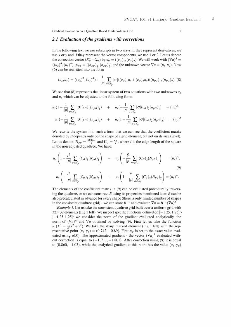
Example 1. Let us take the consistent quadtree grid built over a uniform grid with32×32 elements (Fig.3 left). We inspect specific functions defined on [−1.25,1.25]×[−1.25,1.25]: we consider the norm of the gradient evaluated analytically, thenorm of (∇u)A and ∇u obtained by solving (9). First let us take the functionu1(X) = 1

2 (x2 + y2). We take the sharp marked element (Fig.3 left) with the rep-resentative point (xp,yp) = (0.742,−0.89). First uσ is set to the exact value eval-uated using u(X). The approximated gradient - the vector (∇u)A evaluated with-out correction is equal to (−1,711,−1.801). After correction using (9) it is equalto (0.860,−1.03), while the analytical gradient at this point has the value (xp,yp)

FVCA7, 100, v1 (major): ’Gradient Evalua...’ 5

6 Kriva Zuzana, Handlovicova Angela and Mikula Karol

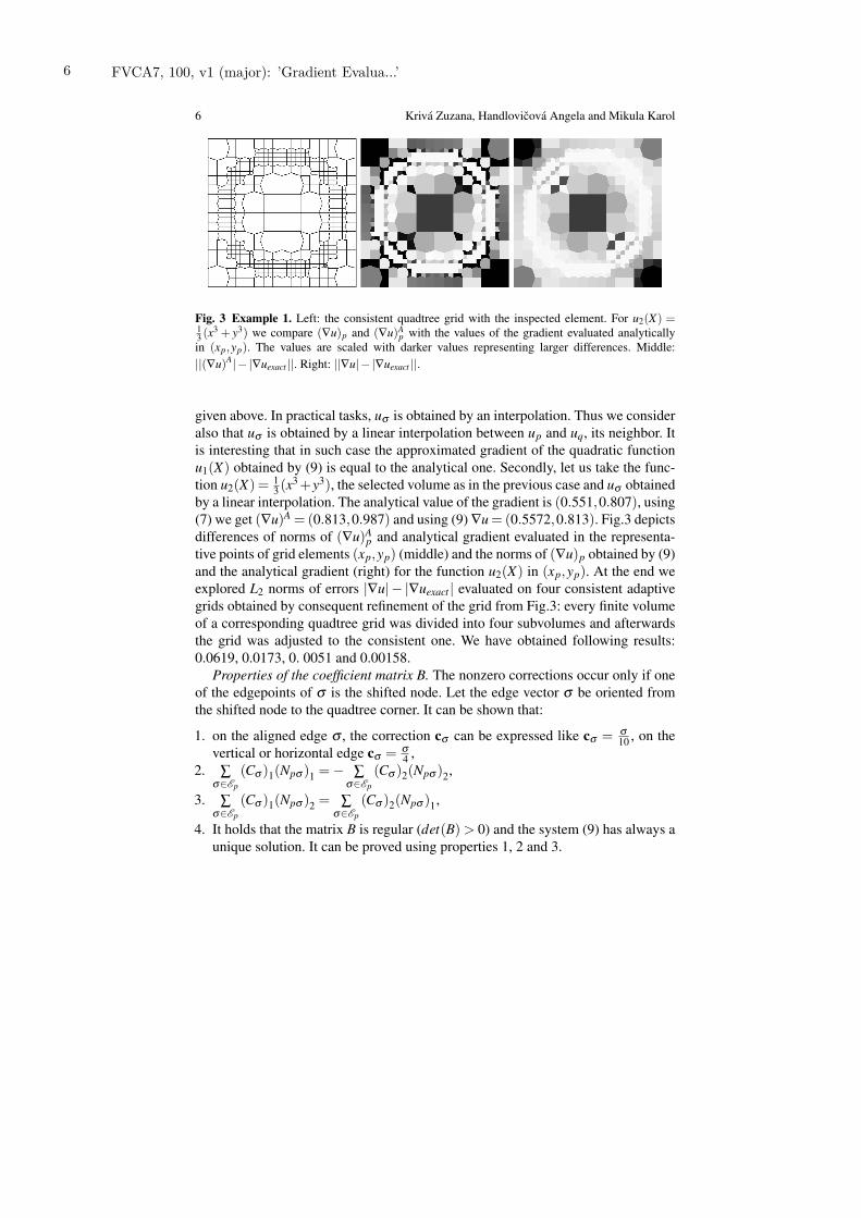
Fig. 3 Example 1. Left: the consistent quadtree grid with the inspected element. For u2(X) =13 (x3 + y3) we compare (∇u)p and (∇u)A

p with the values of the gradient evaluated analyticallyin (xp,yp). The values are scaled with darker values representing larger differences. Middle:||(∇u)A|− |∇uexact ||. Right: ||∇u|− |∇uexact ||.

given above. In practical tasks, uσ is obtained by an interpolation. Thus we consideralso that uσ is obtained by a linear interpolation between up and uq, its neighbor. Itis interesting that in such case the approximated gradient of the quadratic functionu1(X) obtained by (9) is equal to the analytical one. Secondly, let us take the func-tion u2(X) = 1

3 (x3 +y3), the selected volume as in the previous case and uσ obtainedby a linear interpolation. The analytical value of the gradient is (0.551,0.807), using(7) we get (∇u)A = (0.813,0.987) and using (9) ∇u = (0.5572,0.813). Fig.3 depictsdifferences of norms of (∇u)A

p and analytical gradient evaluated in the representa-tive points of grid elements (xp,yp) (middle) and the norms of (∇u)p obtained by (9)and the analytical gradient (right) for the function u2(X) in (xp,yp). At the end weexplored L2 norms of errors |∇u| − |∇uexact | evaluated on four consistent adaptivegrids obtained by consequent refinement of the grid from Fig.3: every finite volumeof a corresponding quadtree grid was divided into four subvolumes and afterwardsthe grid was adjusted to the consistent one. We have obtained following results:0.0619, 0.0173, 0. 0051 and 0.00158.

Properties of the coefficient matrix B. The nonzero corrections occur only if oneof the edgepoints of σ is the shifted node. Let the edge vector σ be oriented fromthe shifted node to the quadtree corner. It can be shown that:

1. on the aligned edge σ , the correction cσ can be expressed like cσ = σ10 , on the

vertical or horizontal edge cσ = σ4 ,

2. ∑σ∈Ep

(Cσ )1(Npσ )1 = − ∑σ∈Ep

(Cσ )2(Npσ )2,

3. ∑σ∈Ep

(Cσ )1(Npσ )2 = ∑σ∈Ep

(Cσ )2(Npσ )1,

4. It holds that the matrix B is regular (det(B) > 0) and the system (9) has always aunique solution. It can be proved using properties 1, 2 and 3.

6 FVCA7, 100, v1 (major): ’Gradient Evalua...’

Gradient Evaluation on a Quadtree Based Finite Volume Grid 7

3 Numerical solution of the regularized Perona-Malik equationon the consistent adaptive grid

In this section we present one experiment - solution of the regularized Perona-Malikequation [1] on a rectangular domain Ω ⊂ IR2 discretized with help of a consis-tent adaptive grid. The scaling interval I = [0,T ] is discretized into scale steps withtn = tn + τ , τ is the scale step size, on the boundaries we keep the zero Neumannboundary conditions. So we solve the problem

∂tu−∇.(g(|∇Gs ∗u|)∇u) = 0, in QT ≡ I ×Ω , (10)

where g(s) = 11+Ks2 , K > 0 is the Perona-Malik function slowing down the diffusion

in the vicinity of edges and Gs(x) is the smoothing kernel. In our algorithm werealize the convolution ∇(Gs ∗u) = Gs ∗∇u by solving the linear heat equation. Weapply one or several steps of the adaptive scheme for time Ts corresponding to s toboth x and y coordinates of the gradient, then we evaluate the norm of the gradientsand apply the Perona-Malik function g to get the diffusion coefficient denoted bygs,n−1

p .Let us denote by un

σ the value of the solution in Xσ at the time step tn. The deriva-

tive in the direction npσ is approximated by ∇un · npσ ≈ (unσ −un

p)dpσ

. The diffusion

coefficient gs,n−1p is constant all over p, thus the flux over σ can be approximated by

Fnpσ = gs,n−1

p|σ |dpσ

(un

σ −unp). (11)

A good way to evaluate |σ |dpσ

is to consider the neighbor q sharing σ with p. Then

we can express (11) with a help of the transmissivity coefficient Tpq = |σ |dpq

and theratio of dpσ and dqσ , where dpσ and dqσ are distances of representative points fromXσ . If σ⊥XpXq in the non adjusted grid, dpσ

dqσ= 1, otherwise, dpσ

dqσ= 4

1 or 14 . For Tpq

it holds that if one edgepoint of σ is a hanging node in the nonadjusted quadtree,then Tpq = 2

3 , otherwise Tpq = 1. The approximated flux (11) can be expressed as

Fnpσ = Tpq

(1+

dqσ

dpσ

)gs,n−1

p(un

σ −unp). (12)

Now we solve the linear system, where the set of equations for all finite volumes p

(unp −un−1

p ) |p| = τ ∑σ∈Ep

Fnpσ (13)

is accompanied by a set of equations for every unσ , σ ∈ Ep, obtained from the rela-

tionship Fnpσ = −Fn

qσ resulting in

FVCA7, 100, v1 (major): ’Gradient Evalua...’ 7

8 Kriva Zuzana, Handlovicova Angela and Mikula Karol

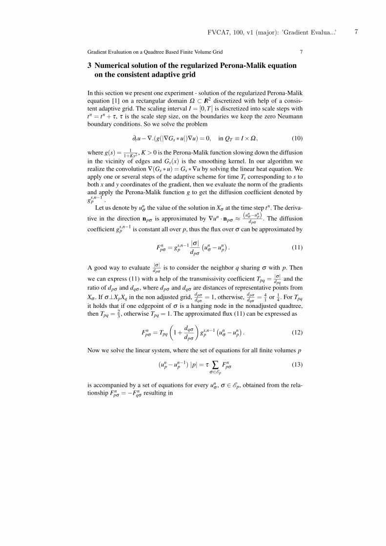
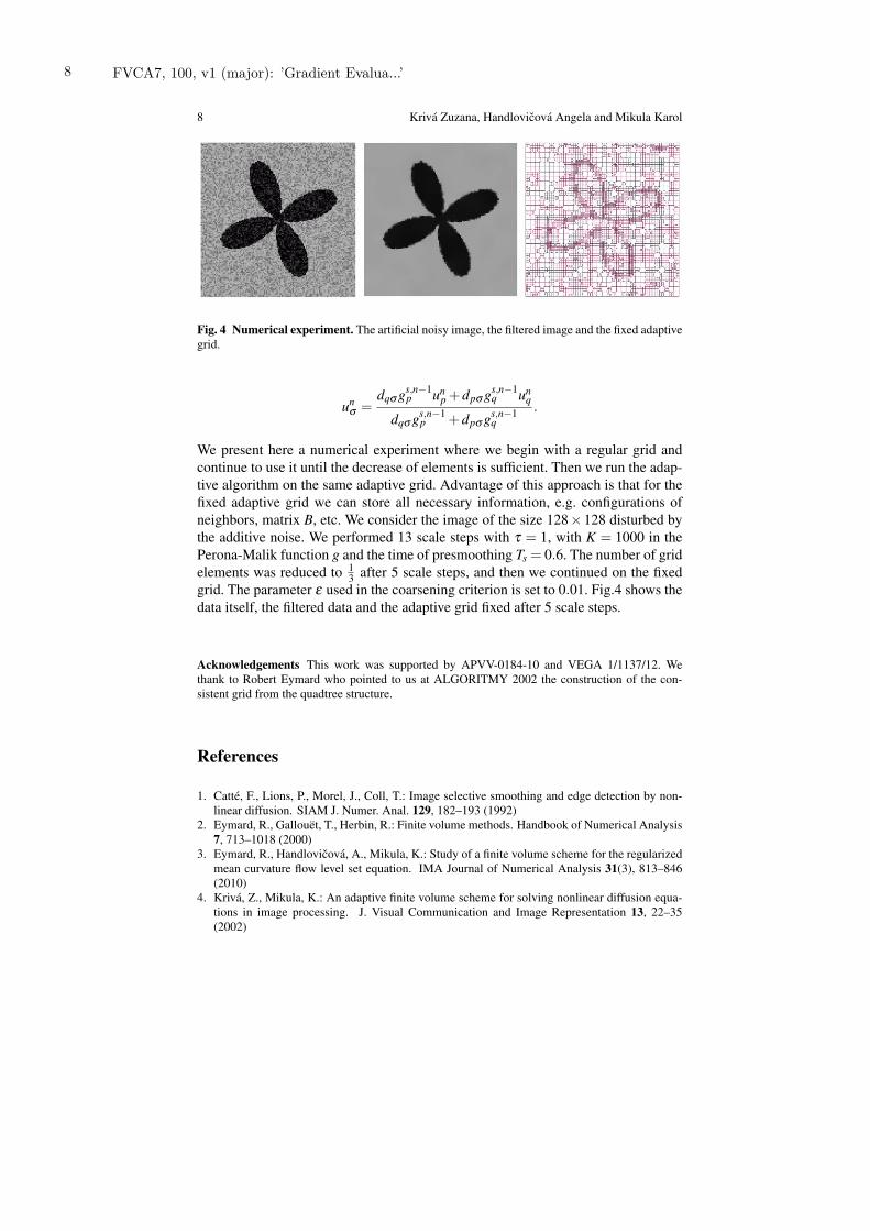
Fig. 4 Numerical experiment. The artificial noisy image, the filtered image and the fixed adaptivegrid.

unσ =

dqσ gs,n−1p un

p +dpσ gs,n−1q un

q

dqσ gs,n−1p +dpσ gs,n−1

q.

We present here a numerical experiment where we begin with a regular grid andcontinue to use it until the decrease of elements is sufficient. Then we run the adap-tive algorithm on the same adaptive grid. Advantage of this approach is that for thefixed adaptive grid we can store all necessary information, e.g. configurations ofneighbors, matrix B, etc. We consider the image of the size 128×128 disturbed bythe additive noise. We performed 13 scale steps with τ = 1, with K = 1000 in thePerona-Malik function g and the time of presmoothing Ts = 0.6. The number of gridelements was reduced to 1

3 after 5 scale steps, and then we continued on the fixedgrid. The parameter ε used in the coarsening criterion is set to 0.01. Fig.4 shows thedata itself, the filtered data and the adaptive grid fixed after 5 scale steps.

Acknowledgements This work was supported by APVV-0184-10 and VEGA 1/1137/12. Wethank to Robert Eymard who pointed to us at ALGORITMY 2002 the construction of the con-sistent grid from the quadtree structure.

References

1. Catte, F., Lions, P., Morel, J., Coll, T.: Image selective smoothing and edge detection by non-linear diffusion. SIAM J. Numer. Anal. 129, 182–193 (1992)

2. Eymard, R., Gallouet, T., Herbin, R.: Finite volume methods. Handbook of Numerical Analysis7, 713–1018 (2000)

3. Eymard, R., Handlovicova, A., Mikula, K.: Study of a finite volume scheme for the regularizedmean curvature flow level set equation. IMA Journal of Numerical Analysis 31(3), 813–846(2010)

4. Kriva, Z., Mikula, K.: An adaptive finite volume scheme for solving nonlinear diffusion equa-tions in image processing. J. Visual Communication and Image Representation 13, 22–35(2002)

8 FVCA7, 100, v1 (major): ’Gradient Evalua...’