Gradient descent - CMU Statisticsryantibs/convexopt-F13/lectures/05-gd.pdf · sublevel set S= fx: f(x) f(x(0))g This is less restrictive 22. Practicalities Stopping rule: stop when

Gradient descent

Barnabas Poczos & Ryan TibshiraniConvex Optimization 10-725/36-725

1

Gradient descent

First consider unconstrained minimization of f : Rn → R, convexand differentiable. We want to solve

minx∈Rn

f(x),

i.e., find x? such that f(x?) = minx f(x)

Gradient descent: choose initial x(0) ∈ Rn, repeat:

x(k) = x(k−1) − tk · ∇f(x(k−1)), k = 1, 2, 3, . . .

Stop at some point

2

●

●

●

●

●

3

●

●

●

●

●

4

Interpretation

At each iteration, consider the expansion

f(y) ≈ f(x) +∇f(x)T (y − x) +1

2t‖y − x‖22

Quadratic approximation, replacing usual ∇2f(x) by 1t I

f(x) +∇f(x)T (y − x) linear approximation to f

12t‖y − x‖

22 proximity term to x, with weight 1/(2t)

Choose next point y = x+ to minimize quadratic approximation:

x+ = x− t∇f(x)

5

●

●

Blue point is x, red point isx+ = argminy∈Rn f(x) +∇f(x)T (y − x) + ‖y − x‖22/(2t)

6

Outline

Today:

• How to choose step size tk

• Convergence under Lipschitz gradient

• Convergence under strong convexity

• Forward stagewise regression, boosting

7

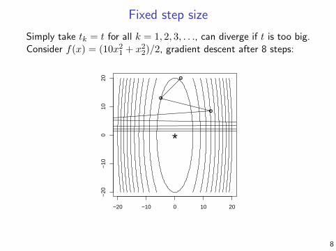
Fixed step size

Simply take tk = t for all k = 1, 2, 3, . . ., can diverge if t is too big.Consider f(x) = (10x21 + x22)/2, gradient descent after 8 steps:

−20 −10 0 10 20

−20

−10

010

20 ●

●

●

*

8

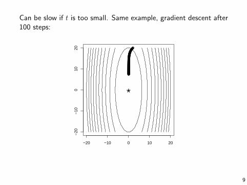
Can be slow if t is too small. Same example, gradient descent after100 steps:

−20 −10 0 10 20

−20

−10

010

20 ●●●●●●●●●●●●●●●●●●●●●●●●●●●●●●●●●●●●●●●●●●●●●●●●●●●●●●●●●●●●●●●●●●●●●●●●●●●●●●●●●●●●●●●●●●●●●●●●●●●●

*

9

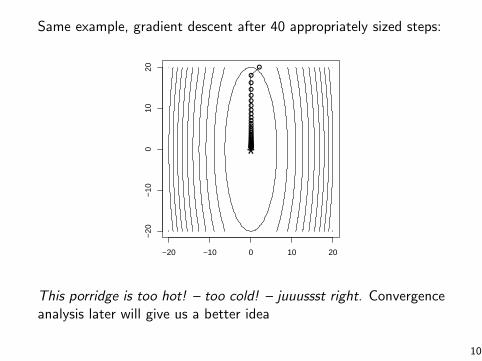
Same example, gradient descent after 40 appropriately sized steps:

−20 −10 0 10 20

−20

−10

010

20 ●

●

●

●●●●●●●●●●●●●●●●●●●●●●●●●●●●●●●●●●●●*

This porridge is too hot! – too cold! – juuussst right. Convergenceanalysis later will give us a better idea

10

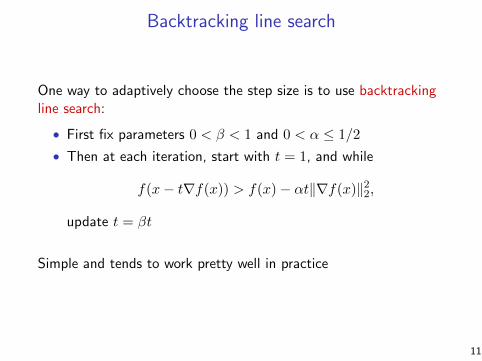
Backtracking line search

One way to adaptively choose the step size is to use backtrackingline search:

• First fix parameters 0 < β < 1 and 0 < α ≤ 1/2

• Then at each iteration, start with t = 1, and while

f(x− t∇f(x)) > f(x)− αt‖∇f(x)‖22,

update t = βt

Simple and tends to work pretty well in practice

11

Interpretation

(From B & V page 465)

For us ∆x = −∇f(x)

12

Backtracking picks up roughly the right step size (13 steps):

−20 −10 0 10 20

−20

−10

010

20 ●

●

●

●

●●

●●

●●

●●●*

Here β = 0.8 (B & V recommend β ∈ (0.1, 0.8))

13

Exact line search

Could also choose step to do the best we can along the directionof the negative gradient, called exact line search:

t = argmins≥0

f(x− s∇f(x))

Usually not possible to do this minimization exactly

Approximations to exact line search are often not much moreefficient than backtracking, and it’s usually not worth it

14

Convergence analysis

Assume that f : Rn → R is convex and differentiable, andadditionally

‖∇f(x)−∇f(y)‖2 ≤ L‖x− y‖2 for any x, y

I.e., ∇f is Lipschitz continuous with constant L > 0

Theorem: Gradient descent with fixed step size t ≤ 1/L satisfies

f(x(k))− f(x?) ≤ ‖x(0) − x?‖22

2tk

I.e., gradient descent has convergence rate O(1/k)

I.e., to get f(x(k))− f(x?) ≤ ε, need O(1/ε) iterations

15

Proof

Key steps:

• ∇f Lipschitz with constant L ⇒

f(y) ≤ f(x) +∇f(x)T (y − x) +L

2‖y − x‖22 all x, y

• Plugging in y = x+ = x− t∇f(x),

f(x+) ≤ f(x)− (1− Lt

2)t‖∇f(x)‖22

• Taking 0 < t ≤ 1/L, and using convexity of f ,

f(x+) ≤ f(x?) +∇f(x)T (x− x?)− t

2‖∇f(x)‖22

= f(x?) +1

2t

(‖x− x?‖22 − ‖x+ − x?‖22

)16

• Summing over iterations:

k∑i=1

(f(x(i))− f(x?)) ≤ 1

2t

(‖x(0) − x?‖22 − ‖x(k) − x?‖22

)≤ 1

2t‖x(0) − x?‖22

• Since f(x(k)) is nonincreasing,

f(x(k))− f(x?) ≤ 1

k

k∑i=1

(f(x(i))− f(x?)

)≤ ‖x

(0) − x?‖222tk

17

Convergence analysis for backtracking

Same assumptions, f : Rn → R is convex and differentiable, and∇f is Lipschitz continuous with constant L > 0

Same rate for a step size chosen by backtracking search

Theorem: Gradient descent with backtracking line search satis-fies

f(x(k))− f(x?) ≤ ‖x(0) − x?‖222tmink

where tmin = min{1, β/L}

If β is not too small, then we don’t lose much compared to fixedstep size (β/L vs 1/L)

18

Strong convexity

Strong convexity of f means for some d > 0,

∇2f(x) � dI for any x

Sharper lower bound than that from usual convexity:

f(y) ≥ f(x) +∇f(x)T (y − x) +d

2‖y − x‖22 all x, y

Under Lipschitz assumption as before, and also strong convexity:

Theorem: Gradient descent with fixed step size t ≤ 2/(d + L)or with backtracking line search search satisfies

f(x(k))− f(x?) ≤ ckL2‖x(0) − x?‖22

where 0 < c < 1

19

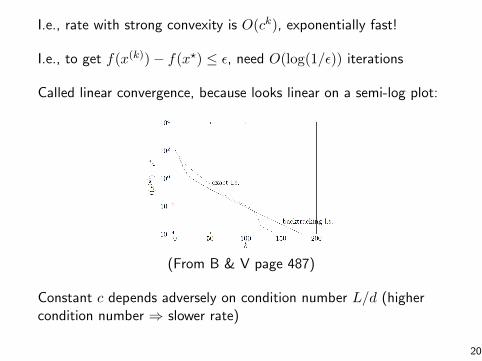
I.e., rate with strong convexity is O(ck), exponentially fast!

I.e., to get f(x(k))− f(x?) ≤ ε, need O(log(1/ε)) iterations

Called linear convergence, because looks linear on a semi-log plot:

(From B & V page 487)

Constant c depends adversely on condition number L/d (highercondition number ⇒ slower rate)

20

A look at the conditions

Lipschitz continuity of ∇f :

• This means ∇2f(x) � LI• E.g., consider f(β) = 1

2‖y −Xβ‖22 (linear regression). Here

∇2f(β) = XTX, so ∇f is Lipschitz with L = σ2max(X)

Strong convexity of f :

• Recall this is ∇2f(x) � dI• E.g., consider f(β) = 1

2‖y −Xβ‖22, with ∇2f(β) = XTX.

Now we need d = σ2min(X)

• If X is wide—i.e., X is n× p with p > n—then σmin(X) = 0,and f can’t be strongly convex

• Even if σmin(X) > 0, can have a very large condition numberL/d = σmax(X)/σmin(X)

21

A function f having Lipschitz gradient and being strongly convexcan be summarized as:

dI � ∇2f(x) � LI for all x ∈ Rn,

for constants L > d > 0

Think of f being sandwiched between two quadratics

This may seem like a strong condition to hold globally, over allx ∈ Rn. But a careful looks at the proofs shows we actually onlyneed to have Lipschitz gradient and/or strong convexity over thesublevel set

S = {x : f(x) ≤ f(x(0))}

This is less restrictive

22

Practicalities

Stopping rule: stop when ‖∇f(x)‖2 is small

• Recall ∇f(x?) = 0

• If f is strongly convex with parameter d, then

‖∇f(x)‖2 ≤√

2dε ⇒ f(x)− f(x?) ≤ ε

Pros and cons of gradient descent:

• Pro: simple idea, and each iteration is cheap

• Pro: Very fast for well-conditioned, strongly convex problems

• Con: Often slow, because interesting problems aren’t stronglyconvex or well-conditioned

• Con: can’t handle nondifferentiable functions

23

Forward stagewise regression

Let’s stick with f(β) = 12‖y −Xβ‖

22, linear regression setting

X is n× p, its columns X1, . . . Xp are predictor variables

Forward stagewise regression: start with β(0) = 0, repeat:

• Find variable i such that |XTi r| is largest, where

r = y −Xβ(k−1) (largest absolute correlation with residual)

• Update β(k)i = β

(k−1)i + γ · sign(XT

i r)

Here γ > 0 is small and fixed, called learning rate

This looks kind of like gradient descent

24

Steepest descent

Close cousin to gradient descent, just change the choice of norm.Let p, q be complementary (dual): 1/p+ 1/q = 1

Steepest descent updates are x+ = x+ t ·∆x, where

∆x = ‖∇f(x)‖q · uu = argmin

‖v‖p≤1∇f(x)T v

• If p = 2, then ∆x = −∇f(x), gradient descent

• If p = 1, then ∆x = −∂f(x)/∂xi · ei, where∣∣∣∣ ∂f∂xi (x)

∣∣∣∣ = maxj=1,...n

∣∣∣∣ ∂f∂xj (x)

∣∣∣∣ = ‖∇f(x)‖∞

Normalized steepest descent just takes ∆x = u (unit q-norm)

25

Equivalence

Normalized steepest descent with respect to `1 norm: updates are

x+i = xi − t · sign( ∂f∂xi

(x))

where i is the largest component of ∇f(x) in absolute value

Compare forward stagewise: updates are

β+i = βi + γ · sign(XTi r), r = y −Xβ

Recall here f(β) = 12‖y −Xβ‖

22, so ∇f(β) = −XT (y −Xβ) and

∂f(β)/∂βi = −XTi (y −Xβ)

Forward stagewise regression is exactly normalized steepest descentunder `1 norm (with fixed step size t = γ)

26

Early stopping and sparse approximation

If we run forward stagewise to completion, then we know that wewill minimize the least squares criterion f(β) = ‖y −Xβ‖22, i.e.,we will get a least squares solution

What happens if we stop early?

• May seem strange from an optimization perspective (wewould be “under-optimizing”) ...

• Interesting from a statistical perspective, because stoppingearly gives us a sparse approximation to the least squaressolution

Well-known sparse regression estimator, the lasso:

minx∈Rp

1

2‖y −Xβ‖22 subject to ‖β‖1 ≤ s

How do lasso solutions and forward stagewise estimates compare?

27

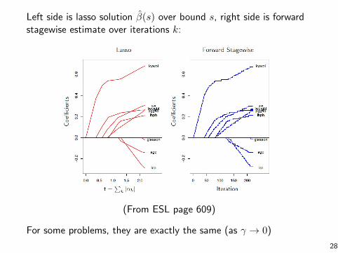
Left side is lasso solution β(s) over bound s, right side is forwardstagewise estimate over iterations k:

(From ESL page 609)

For some problems, they are exactly the same (as γ → 0)

28

Gradient boosting

Given observations y = (y1, . . . yn) ∈ Rn, predictor measurementsxi ∈ Rp, i = 1, . . . n

Want to construct a flexible (nonlinear) model for outcome basedon predictors. Weighted sum of trees:

yi =

m∑j=1

βj · Tj(xi), i = 1, . . . n

Each tree Tj inputs predictor measurements xi, outputs prediction.Trees are grown typically pretty short

...

29

Pick a loss function L that reflects setting; e.g., for continuous y,could take L(yi, yi) = (yi − yi)2

Want to solve

minβ∈RM

n∑i=1

L(yi,

M∑j=1

βj · Tj(xi))

Indexes all trees of a fixed size (e.g., depth = 5), so M is huge

Space is simply too big to optimize

Gradient boosting: basically a version of gradient descent that’sforced to work with trees

First think of minimization as miny f(y), function of predictions y

30

Start with initial model, e.g., fit a single tree y(0) = T0. Repeat:

• Evaluate gradient g at latest prediction y(k−1),

gi =

[∂L(yi, yi)

∂yi

] ∣∣∣∣yi=y

(k−1)i

, i = 1, . . . n

• Find a tree Tk that is close to −g, i.e., Tk solves

mintrees T

n∑i=1

(−gi − T (xi))2

Not hard to (approximately) solve for a single tree

• Update our prediction:

y(k) = y(k−1) + αk · Tk

Note: predictions are weighted sums of trees, as desired

31

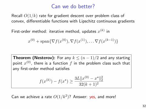
Can we do better?

Recall O(1/k) rate for gradient descent over problem class ofconvex, differentiable functions with Lipschitz continuous gradients

First-order method: iterative method, updates x(k) in

x(0) + span{∇f(x(0)),∇f(x(1)), . . .∇f(x(k−1))}

Theorem (Nesterov): For any k ≤ (n− 1)/2 and any startingpoint x(0), there is a function f in the problem class such thatany first-order method satisfies

f(x(k))− f(x?) ≥ 3L‖x(0) − x?‖2232(k + 1)2

Can we achieve a rate O(1/k2)? Answer: yes, and more!

32

References

• S. Boyd and L. Vandenberghe (2004), “Convex optimization”,Chapter 9

• T. Hastie, R. Tibshirani and J. Friedman (2009), “Theelements of statistical learning”, Chapters 10 and 16

• Y. Nesterov (2004), “Introductory lectures on convexoptimization: a basic course”, Chapter 2

• L. Vandenberghe, Lecture Notes for EE 236C, UCLA, Spring2011-2012

33