GPS tomography of the ionospheric electron content with a correlation functional

GPS Tomography of the Ionospheric ElectronContent with a Correlation FunctionalGiulio Ru�ni�, Alejandro Floresy, Antonio RiuszJanuary 17, 1997AbstractWe develop a minimization functional in order to regularize the inverse prob-lem associated with three-dimensional ionospheric stochastic tomography. Thisfunctional is designed to yield, upon minimization, a solution which maximizesthe frequency content of the solution below a certain cuto�, while keeping �2constant. We show how this functional can be rewritten in terms of the correla-tion function of the image, thereby facilitating the algorithmic implementationof the method. We then implement this functional in a Kalman �lter and obtaina smoothing algorithm that acts in both space and time. Finally, we use thistechnique to perform global scale GPS tomography of the ionospheric electroncontent. KeywordsTomography, Inverse Problem, Ionosphere.�G. Ru�ni is with the Institut d'Estudis Espacials de Catalunya (IEEC), CSIC Research Unit,Edif. Nexus-104, Gran Capit�a 2-4, 08034 Barcelona, Spain. E-mail: ru�[email protected]. Flores is with the Institut d'Estudis Espacials de Catalunya (IEEC), CSIC Research Unit,Edif. Nexus-104, Gran Capit�a 2-4, 08034 Barcelona, Spain. E-mail: [email protected]. Rius is with the Institut d'Estudis Espacials de Catalunya (IEEC), CSIC Research Unit,Edif. Nexus-104, Gran Capit�a 2-4, 08034 Barcelona, Spain. E-mail: [email protected]

1 IntroductionSOLVING the so-called inverse problem consists in choosing a \reasonable" solu-tion for a problem of inversion in which we do not have enough information. Thisis the case, for example, in ionospheric tomography, where one tries to reconstructthe electron density distribution in the ionosphere from satellite delay data. Havingan accurate description of the electron content in the ionosphere is essential to anyendeavor that uses radio wave propagation, since the ionosphere produces delays inthe phase and group propagation of radio waves. E�ects produced by the ionospherea�ect tracking and navigation systems, as well as radio science and radioastronomy|just to name a few. In this paper we describe a technique to perform ionosphericimaging by using the signal delay information provided by the Global PositioningSystem constellation, an area that lately has received considerable attention (see, forexample, [1, 3, 4, 5, 8]).Let �(r; �; �; t) be the function that describes the electron density in some regionof space (r; �; � are spherical coordinates) at some time t. We can rewrite it as�(r; �; �; t) =XJ aJ(t)J(r; �; �) (1)where the functions J(r; �; �) can be any set of basis functions we like. In practice,something like voxels (which will be used here), wavelets or a Fourier expansion arenormally used. The goal in the inverse problem is to �nd the coe�cients aJ(t). In thecase of GPS ionospheric tomography we use the information provided by the GPSdelay data along the satellite-receiver rays li to obtain a set of equations,yi = Zli dl �(r; �; �; t) =XJ aJ(t) Zli dlJ(r; �; �) (2)one for each ray li. Here yi is the observed quantity (see section 4 for details).This is a set of linear equations of the form Ax = y, where the components of the2

vector x are the unknown coe�cients aJ(t). Assume that some cut-o� in the basisfunction expansion is used and, therefore, that the x-space is N -dimensional. Letthe y-space be M -dimensional (M is thus the number of data points). Since thissystem of equations may not have a solution (which will be the case in the followingexperimental situation) we seek to minimize the functional �2(x), where (assuminguncorrelated observations of equal variance)�2(x) = (y � Ax)T � (y � Ax) (3)In practice we �nd that although the number of equations is much greater than thenumber of unknowns, the unknowns are not completely �xed by the data. Thisoccurs partly because the information provided by the data equations is, in general,very repetitive.A very powerful conceptual and practical tool for studying this problem is providedby the Singular Value Decomposition theorem of matrices (SVD)[7], which states thatgiven any M � N matrix A, there exist essentially unique matrices U (M � N), W(N � N), and V (N � N) such that A = U W V T . These matrices have furtherproperties: W is diagonal, with entries bigger or equal to zero, V is orthogonal(V V T = V TV = 1N�N), and the columns of U are orthogonal (UTU = 1N�N). Thepower of this decomposition theorem is that it tells us what the kernel and range of Aare: the kernel of A is spanned by the columns or rows of V which correspond to thezero diagonal elements of W , and the range is spanned by the columns of U whichcorrespond to the nonzero diagonal elements of W . Thus, we have a very useful toolto study the space of solutions of equation (2).In general, there will be many zero diagonal entries in W (the typical examplecorresponding to a voxel that is not hit by any ray); thus, there will be a set of solu-tions to the minimization problem, corresponding to the vector space of homogeneoussolutions (the kernel). The eigenvectors corresponding to the zero eigenvalues repre-sent the un�xed degrees of freedom. The so-called SVD solution is de�ned as the one3

with the minimum norm (see [7]). The general solution is given by the SVD solution(or any other solution) plus an arbitrary linear combination of the eigenvectors cor-responding to zero eigenvalues, x = xSVD +Pi �i vi. How do we choose a solutionout of the many ones available? Let us point out that it would be incorrect to selectone solution and to post-process it (for example by using a smoothing �lter), sincewe would have no control as to which extent the modi�ed solution would depart fromthe information supplied by the data.The proper way to restrict the solution space is to add some a priori constraintsto the problem, and this can be implemented using the Lagrange multiplier method.This method says that extremization of the function �2(x) subject to the constraint�(x) = 0 can be done by extremizing G(x) = �2(x) + ��(x), with � varied as well.However, if we �x � to some arbitrary value �0 and extremize G(x) = �2(x)+�0�(x)with respect to x, the extremum that we �nd, x0, is what we would get by solvingthe problem of extremizing �2(x) holding �(x) � �(x0) = 0. Note that the rolesof the � and �2 can be exchanged: we could instead say that the constraint is�2(x) � �2(x0) = 0, and minimize �(x), with the same result. If the functionalextremization is to be performed numerically using a minimization algorithm, it isalso important that we de�ne G(x) so that the extremum is a minimum. For example,if we tried to implement the extremization procedure using the multiplier as anotherunknown, we would �nd that the functional has no minimum, only an extremum|thefunctional's Hessian matrix is not positive de�nite.In the case of stochastic ionospheric tomography it is natural to use smoothingconstraints, since one may be trying to describe the problem with many more voxels(degrees of freedom) than e�ective data measurements. It seems reasonable to askthat the images have some �nite resolution|ideally re ecting the real resolution ofthe measuring instrument.A possible smoothing constraint is provided by the concept of relative entropy,R. Here we discuss brie y one method we have devised using this concept, since it4

provides an interesting contrast to the correlation functional approach which we willpresent later. Entropy methods have been used before (see, for example [2],[7]). Letx be the vector that describes the voxel representation of the image. The relativeentropy of the image is then de�ned by (assuming voxels of equal volume)R(x) = 1log(1=N)Xi jxijT log jxijT (4)where T = Pi jxij, and N is the number of voxels. This function (which is a numberbetween 0 and 1) counts the number of ways in which one could construct the imagestarting from a normalized quantity of electrons, and is independent of the number ofvoxels. A totally smooth image has a relative entropy of 1, and one in which all theelectrons are concentrated in one voxel has a relative entropy of 0. The use of entropyoriginates in the question \Given the data and the geometry of the imaging array, whatis the most probable electron distribution that would have generated it?" Here the term\probable" is meant in the statistical mechanical sense: a distribution x is consideredmore probable the smaller the value of �2(x) it yields, and the larger the number ofways to produce it is (in the combinatorial sense). The solution image x is then de�nedas the one that maximizes the probability function, P(x; �; �) = exp(�G(x; �; �)),with G(x; �; �) = �2(x)� � R(x) + �2 (T � T0)2 (5)(the last term allows us to specify the total number of electrons in the image1). HereT0 is a constant (T = Pi jxij, as de�ned above). This term is needed to counteract theentropic tendency to increase the electron density of the image, and acts to stabilizethe minimization process.1This is a standard statistical mechanical line of reasoning. Here �2(x) plays the role of theenergy and G(x; �) = �2(x) � � R(x) + �2 (T � T0)2 the free energy, with � being the temperatureand � the chemical potential. 5

Since the extremization equation for this functional is not linear we have chosento minimize this functional using the Broyden-Fletcher-Goldfarb-Shanno algorithm(see [7], for example).Despite the usefulness of the entropic approach in many applications, it has animportant shortcoming if it is to be used as a smoothing method. Indeed, the mea-surement of entropy of a distribution cannot take into account any local consider-ations of smoothness. For example, the images fxig and fx�(i)g, where �(i) is anarbitrary permutation of the voxels, have the same entropy. Also, the nonlinearityof the equations associated with this functional means that the minimization has tobe performed numerically directly on the functional, as opposed to a simple linearinversion of the zero-gradient equations|which will be the case if the functional is asimple quadratic|and this is a computationally intensive task. For these reasons wehave not attempted to implement this method in a Kalman �lter. The correlationfunctional which we develop next produces similar results to the entropic one, butenforces real spatial smoothness and it is quadratic.2 The Correlation functionalThe functional we wish to discuss here uses local information: the smoothness of theimage is quanti�ed by measuring local correlations. However, we can best motivatethis functional by using Fourier analysis. The idea is that we want to limit the spatialresolution of our image, and at the same time keep �2 �xed to some value. This canbe achieved by asking that the power spectrum of the image be as concentrated aspossible in a speci�ed volume of frequencies around the origin. By doing this we limitthe resolution of the image: of all the images with the same �2 we will choose thosethat can be described by a Fourier series with a frequency cuto�, that is, those withthe least detail beyond a speci�ed scale. Let Px(~k) be the power spectrum of theimage, 6

Px(~k) = �����Z d3r(2�)3=2 x(~r) e�i~k�~r�����2 (6)The power spectrum content of the image outside a cube in frequency space withsides 2�i (i.e., the high portion of the spectrum) is then given byQhx(~�) = Z d3r (x(~r))� x(~r)� Z dk3H�(~k)Px(~k) (7)where the function H� limits the k integral to a box of sides 2�i centered at the origin.This is the term that we seek to minimize|note that it is bounded from below. Thecontinuum functional that implements this is (recall that here x(~r) plays the role ofthe density) G(x; �; �) = �2(x) + �Qhx(~�) + �2 �Z d3r x(~r)� T0�2 (8)The last term is used to control the total image content. The resolution in anydirection, say ri, is then given by �ri � �i � 1. Moreover, the resolution requirementis enforced to the extent that the data does not specify the image values at the voxels.If, for instance, a neighborhood of voxels is well-determined by the data, the �2(x)contribution to the functional will dominate the solution there. In this sense we cansay that there is a local enforcement of the resolution requirement which depends onthe data.Let us now see how we can rewrite this functional in terms of the correlationfunction. Recall that the cross-correlation function between two functions is given byRf;g(~h) = hf(~z)g(~z + ~h)i~z = Z d3z f(~z)g(~z + ~h) (9)Now, the Fourier transform of the auto-correlation function for a function f(~r) is justits power spectrum (let f� denote f(�~r), and � the usual convolution of functions),7

F [Rf;f ] = F [f � f�] = F [f ] � F [f�] = Px(~k) (10)Hence we can rewrite the low portion of the spectrum,Qlx(~�) � Z dk3H�(~k)Px(~k) = Z dk3H�(~k) � F [Rf;f ](~k) (11)Let b�(~r) be the inverse Fourier transform of H�(~k). ThenQlx(~�) = Z dk3H�(~k) � F [Rf;f ](~k)= Z dr3 b�(~r) �Rf;f(~r) (12)(since Rf;f(~r) is even) and we can rewrite the functional in equation (8),G(x; �; �) = �2(x) + � Z d3r Rx;x(~r) [�3(~r)� b�(~r)] + �2 �Z d3r x(~r)� T0�2 (13)Now, let Ni be the number of voxels in the ri direction. Since the image space isbounded, b�(~r) is given by the Fourier series generated by H�, the function thatde�nes the cube in frequency space (ki = ni2�=Ni),b�(~r) = 3Yi=1 1Ni! X~k2Box� ei~k�~r = 3Yi=1 sin( 2�Ni (nmaxi + 1=2)ri)Ni sin( �Ni ri) (14)where �i = 2�nmaxi =Ni. Note that we are using \pixel units"to measure length, where�i = Li=Ni equals one pixel unit in the i direction. In terms of the �nite size of theimage and the digital nature of the reconstruction, the former expressions turn out tobe as follows. The autocorrelation function for a voxel 3D image x � Xi;j;k is givenby the circular sum Rx;xmnl = Xi;j;kXi;j;kXi+m;j+n;k+l (15)8

(where the sum over the indices wraps around if needed), and the the other term inthe integral in equation (13) is given by the sum� Z d3r Rx;x(~r) b�(~r) = �XmnlRx;xmnl b�lmn (16)with (let l1 = l; l2 = m; l3 = n)b�lmn = Z l+1l dr1 Z m+1m dr2 Z n+1n dr3 b�(~r)= 3Yi=10@ 1Ni + 2 nmaxiXni=1 sin(ni�=Ni)ni� cos(2�ni(li + 12)=Ni)1A (17)Now the G(x; �; �) functional adopts the following form:G(x; �; �) = �2(x) + � Xl;m;nRx;xlmn [�l0�m0�n0 � b�lmn] + �2 0@Xl;m;nXlmn � T01A2= �2(x) + � Xi;j;k;l;m;nXijk[�il�jm�kn � B�(ijk)(lmn)]Xlmn + �2 0@Xl;m;nXlmn � T01A2= �2(x) + �XI;J XI [�IJ � B�IJ ]XJ + �2 XI XI � T0!2 (18)where the symmetric matrix B� is given byB�(ijk)(lmn) = 12 �b�i�m;j�n;k�l + b�m�i;n�j;l�k� = 12 �b�I�L + b�L�I� (19)and the last expression is symbolic shorthand2. The associated pixel resolution inany direction is given by Ri � Ni=�i = Ni=2�nmaxi .Taking the derivative of the above functional and setting it equal to zero yieldsthe equation2To be precise we mean MLQ �M(ijk);(lmn) and b�L�Q � b�i�l;j�m;k�n9

�ATA+ �(I �B�) + �T�x = ATy + �T0 (20)where TIJ = 1 and B�LQ = (b�Q�L + b�L�Q)=2 was de�ned above. Now, let S =ATA+ �(I �B�) + �T , a symmetric matrix. The covariance matrix associated withx is given by the inverse Hessian of the functional, Cx = S�1.3 Implementation with a Kalman �lterKalman �ltering is a very useful technique when dealing with a dynamic process inwhich data is available for di�erent times. It is a natural way to enforce smoothnessunder time evolution, and is especially useful in the case of ionospheric stochastictomography, when the \holes" in the information that we may have at a given time(because of the particular spatial distribution of the measuring instrument, the GPSconstellation and the receptor grid) may be \plugged" by the data from previous andfuture measurements. Indeed, in a Kalman �lter we use the information containedin a solution to the inversion problem to estimate the next solution in the iterationprocess. In the study of the ionosphere, for example, we break the continuous ow ofsatellite delay data into blocks of a few hours, and model the dynamics by a randomwalk [6]. We can then process the data at a given point in the iteration by askingthat, to some extent, the solution be similar to the one in the previous iteration:how similar, depends on how much con�dence we had in that previous solution, andon how much we expect the dynamics to have changed things from one solution tothe next. In other words, if xn and Cxn(= S�1n ) are the solution and the covariancematrix at epoch n, at epoch n + 1 we are to minimizeKn+1 = Gn+1(xn+1; �; �) + � (xn+1 � xn)T �Cxn + �2��1 (xn+1 � xn) (21)with respect to xn+1. The parameter � expresses our con�dence in the previous10

solution, while � (which will in general be a diagonal N � N matrix) models therandom walk away from it. Minimization yieldsxn+1 = �Sn+1 + � �S�1n + �2��1��1 �ATn+1yn+1 + �T0 + � �S�1n + �2��1 xn� (22)which can be easily implemented in an algorithm. A value of � = 1 will be used here,which is the case in standard Kalman �ltering.4 Application to GPS Ionospheric tomographyIn this section we apply the above methods to study the ionosphere. The use of theGPS constellation to study the ionosphere is hardly new (see [3, 8] for an example ofthe use of the GPS constellation to produce ionospheric maps, and [3] for a discussionof GPS ionospheric tomography), but here we will be using a large amount of data (60receiving stations) as well as novel techniques to produce real, global, tomographic\snapshot" images of the ionosphere.The GPS observables consist essentially of the delays experienced by the dualfrequency signals (f1 =1.57542 GHz and f2 =1.22760 GHz) transmitted from the GPSconstellation (25 satellites) and received at GPS receivers around the world. Let Li bethe measured total ight time in light-meters of a ray going between a given satelliteand receiver at the frequency fi (including instrumental biases), and I = Rray dl �(~x)be the integrated electron density along the ray (in electrons per square meter). ThenLi is modeled by Li = D� I �=f 2i +~csat+~crec, where � = 40:3m3=s2, D is the lengthof the ray, and ~csat and ~crec are the instrumental biases. In the present case we areinterested in the frequency dependent part of the delay: L = L1�L2 (in meters). Thisis the derived observable and is modeled by ( = 1:05�10�17 m3) L = I+csat+crec,independent of D (see [1] for more details). Here, phase center o�sets have alreadybeen accounted for (models for the antenna phase center o�sets have been used toremove systematic errors) and sources of error like multi-path e�ects are neglected,11

because we will not include data below a cuto� elevation angle of 15o, and becausethey have little e�ect on the real resolution of the GPS constellation and receptorgrid.Because solar radiation is the major agent shaping the ionosphere and drivingits evolution, we use a sun-�xed coordinate system to describe it. The referenceplane is the equator and the origin of longitudes is chosen so that the Sun is at180o (this coordinate system coincides approximately with the usual geographicallatitude/longitude coordinate system at UT 00).The GPS data has been collected from a subset of the International GPS Service(IGS) Network (see �gure 1, 2), for the day of October 18th, 1995, between the hoursof UT 02 and UT 22. This particular day has been chosen for its high geomagneticand solar activity indices (as distributed by the US National Geophysical Data Center(NGDC) and the National Space Science Data Center (NSSC), as well as for the sud-den decrease in the electron content measurements provided by the GeosynchronousOperational Environmental Satellites (GOES) (as supplied by the NGDC). The rawdata has been pre-processed in order to obtain the observables using the proceduresdescribed in [1]. For the purposes of analysis the data has then been broken in 10blocks of two hours each, during which the ionosphere is presumed to have been static.To describe the ionosphere we use two geocentric spherical layers 150 km thick,beginning at 200 km above the mean surface of the Earth. Each layer consists then ofone hundred voxels of dimensions 18o in latitude, times 36o in longitude, times 150 kmof height. At this stage of research, we have chosen this grid size for computationalconvenience, and the height of the two layers accounts for the major portion of theionospheric electron content. Other grid sizes and distributions are certainly possible,including the addition of more layers. The unknowns here consist of the electrondensities at each of these voxels, plus the 85 unknowns corresponding to the satelliteand receptor constant delays.In �gure 3 we can see an example of the use of the entropic and correlation12

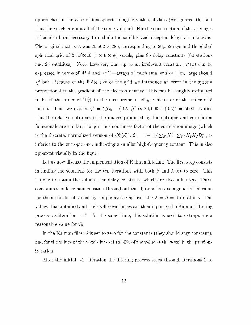
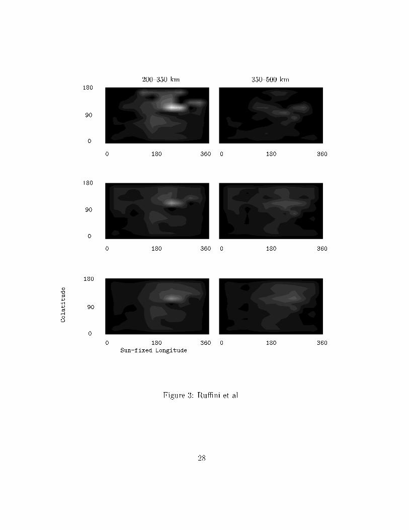
approaches in the case of ionospheric imaging with real data (we ignored the factthat the voxels are not all of the same volume). For the construction of these imagesit has also been necessary to include the satellite and receptor delays as unknowns.The original matrix A was 20,562 � 285, corresponding to 20,562 rays and the globalspherical grid of 2�10�10 (r � � � �) voxels, plus 85 delay constants (60 stationsand 25 satellites). Note, however, that up to an irrelevant constant, �2(x) can beexpressed in terms of ATA and ATY|arrays of much smaller size. How large should�2 be? Because of the �nite size of the grid we introduce an error in the systemproportional to the gradient of the electron density. This can be roughly estimatedto be of the order of 10% in the measurements of y, which are of the order of 5meters. Thus we expect �2 = P(yi � (AX)i)2 � 20; 000 � (0:5)2 = 5000. Noticethat the relative entropies of the images produced by the entropic and correlationfunctionals are similar, though the smoothness factor of the correlation image (whichis the discrete, normalized version of Qhx(~�)), C = 1 � [1=PK X2K ]PIJ XIXJB�IJ , isinferior to the entropic one, indicating a smaller high-frequency content. This is alsoapparent visually in the �gure.Let us now discuss the implementation of Kalman �ltering. The �rst step consistsin �nding the solutions for the ten iterations with both � and � set to zero. Thisis done to obtain the value of the delay constants, which are also unknowns. Theseconstants should remain constant throughout the 10 iterations, so a good initial valuefor them can be obtained by simple averaging over the � = � = 0 iterations. Thevalues thus obtained and their self-covariances are then input to the Kalman �lteringprocess as iteration \-1". At the same time, this solution is used to extrapolate areasonable value for T0.In the Kalman �lter � is set to zero for the constants (they should stay constant),and for the values of the voxels it is set to 30% of the value at the voxel in the previousiteration.After the initial \-1" iteration the �ltering process steps through iterations 1 to13

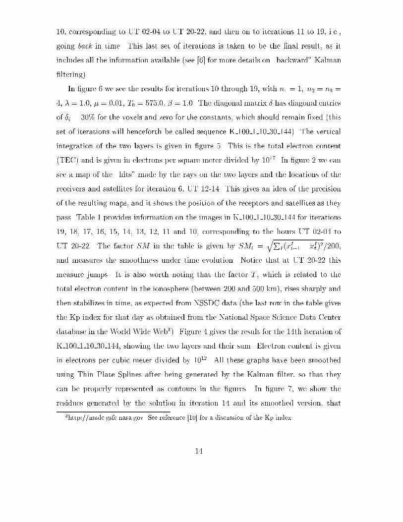
10, corresponding to UT 02-04 to UT 20-22, and then on to iterations 11 to 19, i.e.,going back in time. This last set of iterations is taken to be the �nal result, as itincludes all the information available (see [6] for more details on \backward" Kalman�ltering).In �gure 6 we see the results for iterations 10 through 19, with n1 = 1; n2 = n3 =4, � = 1:0, � = 0:01; T0 = 575:0, � = 1:0. The diagonal matrix � has diagonal entriesof �i = 30% for the voxels and zero for the constants, which should remain �xed (thisset of iterations will henceforth be called sequence K 100 1 10 30 144). The verticalintegration of the two layers is given in �gure 5. This is the total electron content(TEC) and is given in electrons per square meter divided by 1017. In �gure 2 we cansee a map of the \hits" made by the rays on the two layers and the locations of thereceivers and satellites for iteration 6, UT 12-14. This gives an idea of the precisionof the resulting maps, and it shows the position of the receptors and satellites as theypass. Table 1 provides information on the images in K 100 1 10 30 144 for iterations19, 18, 17, 16, 15, 14, 13, 12, 11 and 10, corresponding to the hours UT 02-04 toUT 20-22. The factor SM in the table is given by SMt = qPI(xIt+1 � xIt )2=200,and measures the smoothness under time evolution. Notice that at UT 20-22 thismeasure jumps. It is also worth noting that the factor T , which is related to thetotal electron content in the ionosphere (between 200 and 500 km), rises sharply andthen stabilizes in time, as expected from NSSDC data (the last row in the table givesthe Kp index for that day as obtained from the National Space Science Data Centerdatabase in the World Wide Web3). Figure 4 gives the result for the 14th iteration ofK 100 1 10 30 144, showing the two layers and their sum. Electron content is givenin electrons per cubic meter divided by 1012. All these graphs have been smoothedusing Thin Plate Splines after being generated by the Kalman �lter, so that theycan be properly represented as contours in the �gures. In �gure 7, we show theresidues generated by the solution in iteration 14 and its smoothed version, that3http://nssdc.gsfc.nasa.gov. See reference [10] for a discussion of the Kp index.14

is, the di�erences between the predicted and actual delays for the rays. As can beinferred from the histogram, the residues are of the order of 30 cm|a bit better thanexpected. This could certainly be improved if a �ner grid were used, since the mainsource of error comes from the \digitization" of the solutions. The smoothed outversions of the solution yield slightly smaller residues (about 3 centimeters less onthe average).5 Summary, ConclusionsWe have discussed the use of statistical considerations and smoothness conditionsas a priori information (i.e., auxiliary constraints) to �x the solution in the inverseproblem of stochastic tomography. Such approaches have proved useful in the past inthe context of modeled and real data, yielding more complete and realistic solutionsthan the minimum-norm SVD approach [7], for example. This is especially true whenthe images have characteristic scales larger than the grid being used, and when thedata has \holes"|which is the case in ionospheric stochastic tomography.Ideally, one would like to implement four dimensional smoothing equations, withan e�ect in both space and time. In practice, this may turn out to be a computation-ally impractical approach, and here we have have chosen to do the next best thing:Kalman �ltering with a smoothing functional.We have argued that the correlation method provides a potentially superior smooth-ing algorithm to the entropic one, as the measurement of the entropy of a distributioncannot take into account any local considerations of smoothness. For example, theimages fxig and fx�(i)g, where �(i) is an arbitrary permutation of the voxels, havethe same entropy. The correlation functional can distinguish the two.Moreover, the minimization of the correlation functional can be written as a linearequation, which allows it to be easily implemented in a Kalman �lter. The result is asmoothing process in space and in time that takes into account the dynamic natureof the estimates and covariances produced by the data.15

We have then successfully tested these methods with the study of the electroniccontent of the ionosphere at a global scale (albeit with a coarse grid), thus comple-menting other sources of information like GOES, and providing additional experimen-tal data which can be used in existing ionospheric models (such as the InternationalReference Ionosphere model (IRI) [9]). The results suggest that this method can bepotentially very useful when employed with �ner grids, a task already underway.AcknowledgmentsThe authors would like to acknowledge the collaboration of Jos�e Miguel Juan, ManuelHernandez and Jaume Sanz of the Polytechnic University of Catalonia in the datapre-processing, as well as their valuable comments and criticism. G.R. wishes to thankJulianne Chisholm for careful proofreading, Rod Glenister of JPL , Mark Fallis, PaulAnderson and Chuck Deleone of UC Davis, and Gary Oas of Stanford University formany stimulating discussions on this and related subjects.

16

References[1] E.Sard�on, A.Rius, N. Zarraoa, Estimation of the transmitter and receiver di�er-ential biases and the ionospheric total electron content from Global PositioningSystem observations, Radio Science, 29(3):577{586, 1994.[2] L.R.D'Addario, S.J.Wernecke, Maximum entropy image reconstruction, IEEETransactions on Computers, C-26(4), April 1977.[3] G.A. Hajj, R. Ibanez-Meir, E.R. Kursiniski, L.J. Romans, Imaging the Ionospherewith the Global Positioning System, International Journal of Imaging Systemsand Technology, Vol. 5, 174-184, 1994[4] A.J. Manucci, B.D. Wilson, C.D Edwards, A new method for monitoring theEarth's ionospheric total electron content using the GPS global network, Proc. ofthe Institute of Navigation GPS-93, Salt Lake City, Utah, Sept 22-24, 1993[5] H. Na, E. Sutton, Resolution Analysis of Ionospheric Tomography Systems, In-ternational Journal of Imaging Systems and Technology, Vol. 5(2):169{173, 1994.[6] T.A. Herring, J.L. Davis, I.I.Shapiro, Geodesy by radio interferometry: Theaplication of kalman �ltering to the analysis of very long baseline interferometrydata, Journal of Geophysical Research, 95(B8):12,561{12,581, August 1990.[7] S A Teukolsky, W H Press, W T Vettering, Flannery, Numerical Recipes inFortran, The Art of Scienti�c Computing, Cambridge University Press, 1994.[8] B.D. Wilson, A.J. Manucci, C.D. Edwards, Subdaily northern hemisphere iono-spheric maps using an extensive network of GPS receivers, Radio Science, Vol.30(3):639{648, 1995.[9] D. Bilitza (ed.), Reference Ionosphere 1990, NSSDC Report 90-22, US NationalSpace Science Data Center Maryland, 1990[10] K. Davies, Ionospheric Radio, IEE Electromagnetic Waves Series 31, PeterPeregrinus Ltd., London, UK

17

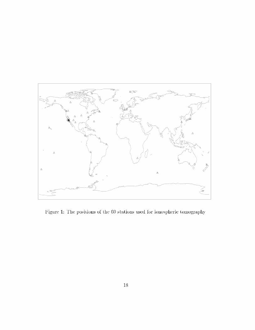
Figure 1: The positions of the 60 stations used for ionospheric tomography.

18

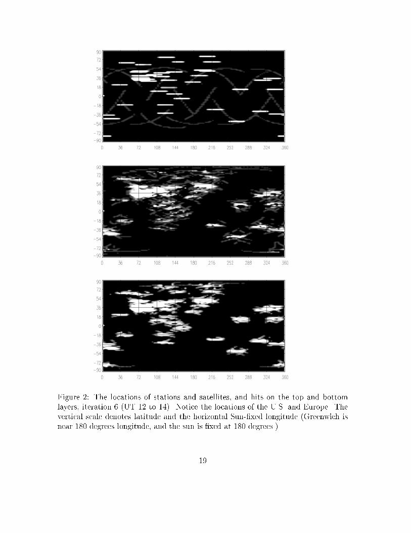
Figure 2: The locations of stations and satellites, and hits on the top and bottomlayers, iteration 6 (UT 12 to 14). Notice the locations of the U.S. and Europe. Thevertical scale denotes latitude and the horizontal Sun-�xed longitude (Greenwich isnear 180 degrees longitude, and the sun is �xed at 180 degrees.)19

Sun-fixed Longitude0 180 360 0 180 360090180

Colatitude

200{350 km 350{500 km180900180900 0 180 360 0 180 360

0 180 360 0 180 360

Figure 3: In this sequence of images we see the plain SVD solution (top), the solutionusing the entropy functional (middle), and the one using correlations (bottom), withn1 = 1; n2 = n3 = 2, � = 1:9, and � = 20:0; T0 = 550:0. The two slices in each imagecorrespond to a height of 200-350 (left) and 350-500 (right) km above the ground. Onthe vertical scale, the colatitude varies from 0 to 180 degrees, and on the horizontalthe sun-�xed longitude from 0 to 360. The grid is made out of 2�10�10 voxels. Thevalues of �2, relative entropy R, correlation C = 1� [1=PK X2K ]PIJ XIXJB�IJ , andT = P jxij for the three images (top, middle, bottom) are (5468, 0.910, 0.42, 478),(5709, 0.976, 0.12, 550), and (5712, 0.975, 0.07, 550) respectively.20

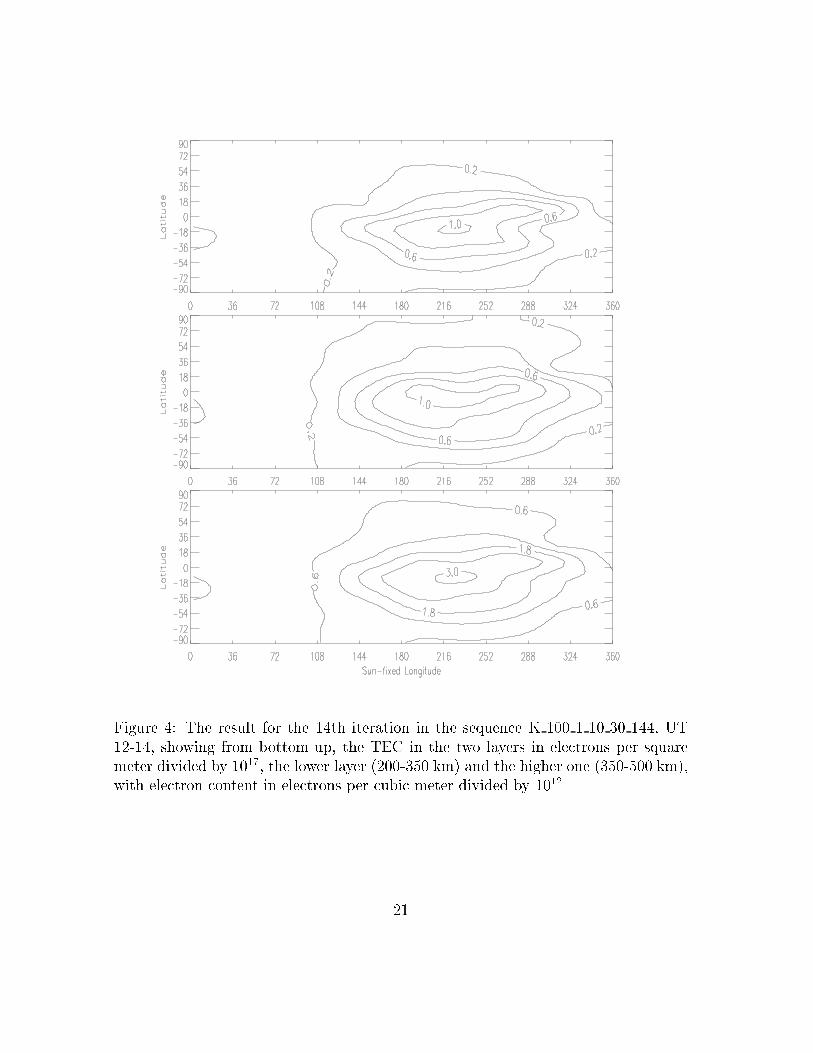
Figure 4: The result for the 14th iteration in the sequence K 100 1 10 30 144, UT12-14, showing from bottom up, the TEC in the two layers in electrons per squaremeter divided by 1017, the lower layer (200-350 km) and the higher one (350-500 km),with electron content in electrons per cubic meter divided by 1012.21

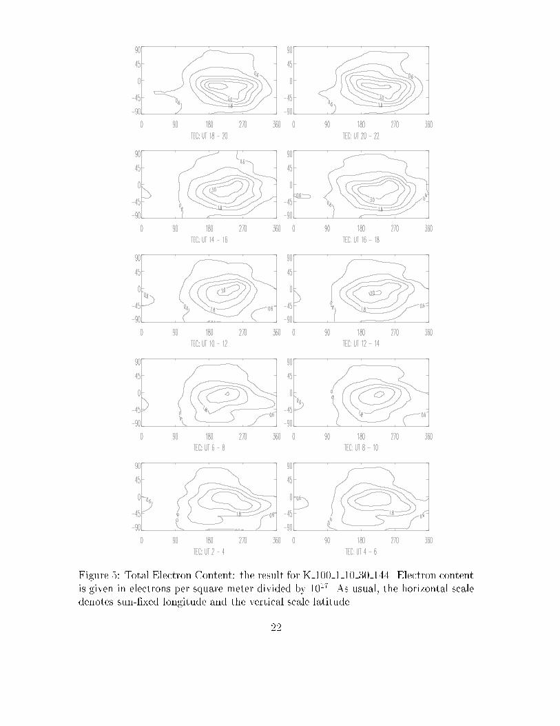
Figure 5: Total Electron Content: the result for K 100 1 10 30 144. Electron contentis given in electrons per square meter divided by 1017. As usual, the horizontal scaledenotes sun-�xed longitude and the vertical scale latitude.22

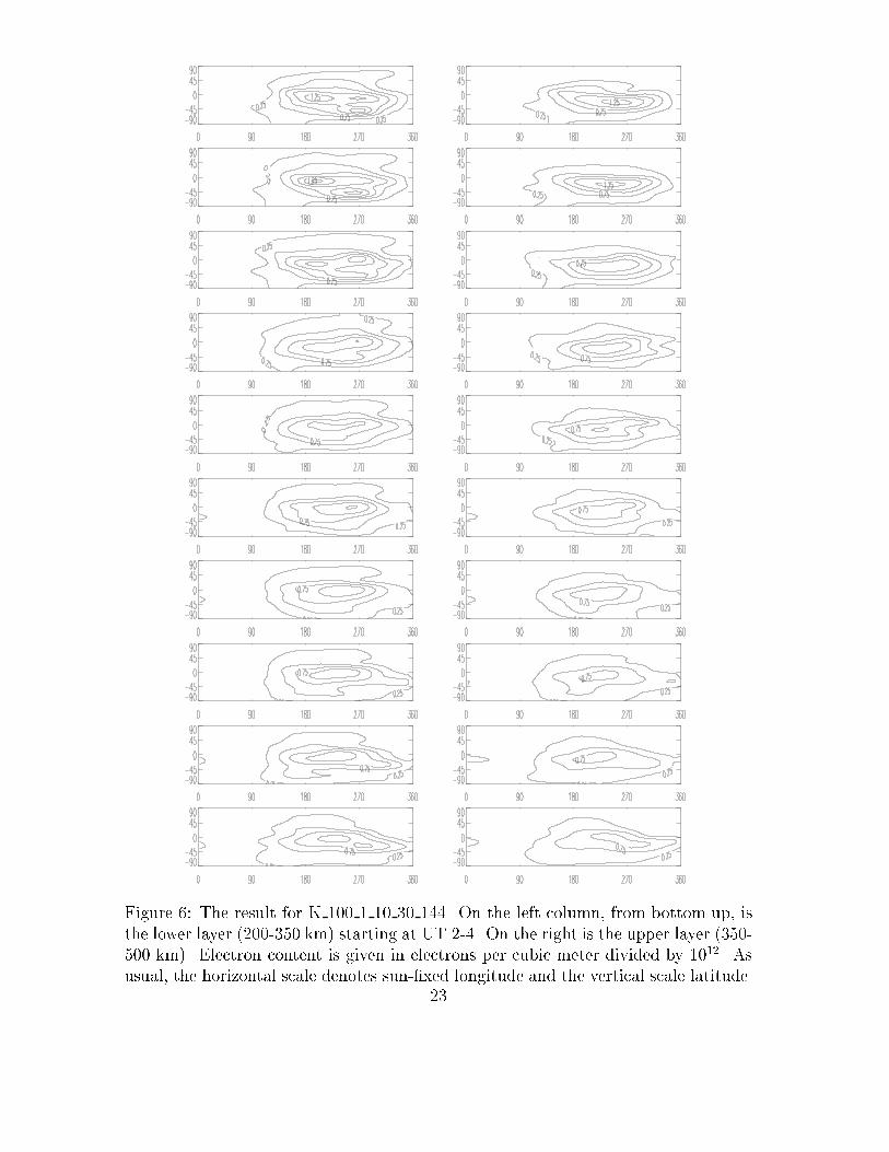
Figure 6: The result for K 100 1 10 30 144. On the left column, from bottom up, isthe lower layer (200-350 km) starting at UT 2-4. On the right is the upper layer (350-500 km). Electron content is given in electrons per cubic meter divided by 1012. Asusual, the horizontal scale denotes sun-�xed longitude and the vertical scale latitude.23

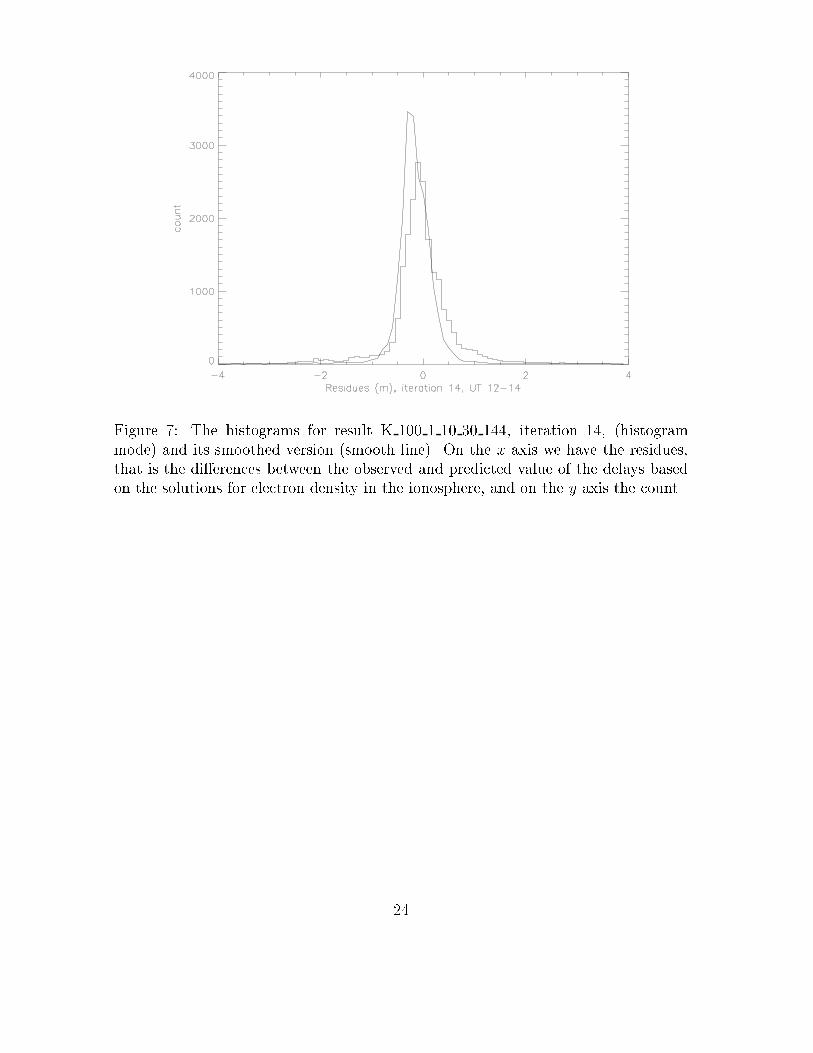
Figure 7: The histograms for result K 100 1 10 30 144, iteration 14, (histogrammode) and its smoothed version (smooth line). On the x axis we have the residues,that is the di�erences between the observed and predicted value of the delays basedon the solutions for electron density in the ionosphere, and on the y axis the count.

24

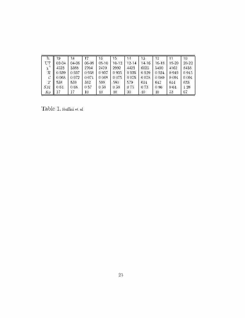
It. 19 18 17 16 15 14 13 12 11 10UT 02-04 04-06 06-08 08-10 10-12 12-14 14-16 16-18 18-20 20-22�2 4523 3388 2704 2470 2992 4423 6025 5490 4162 8438R 0.939 0.937 0.938 0.937 0.935 0.935 0.929 0.924 0.919 0.915C 0.068 0.072 0.071 0.068 0.075 0.075 0.078 0.089 0.091 0.091T 558 559 562 569 580 579 614 642 614 633SM 0.64 0.68 0.57 0.59 0.59 0.75 0.73 0.86 0.64 1.28Kp 17 17 10 40 40 30 40 40 53 67Table 1, Ru�ni et al.

25

Figure 1: Ru�ni et al.

26

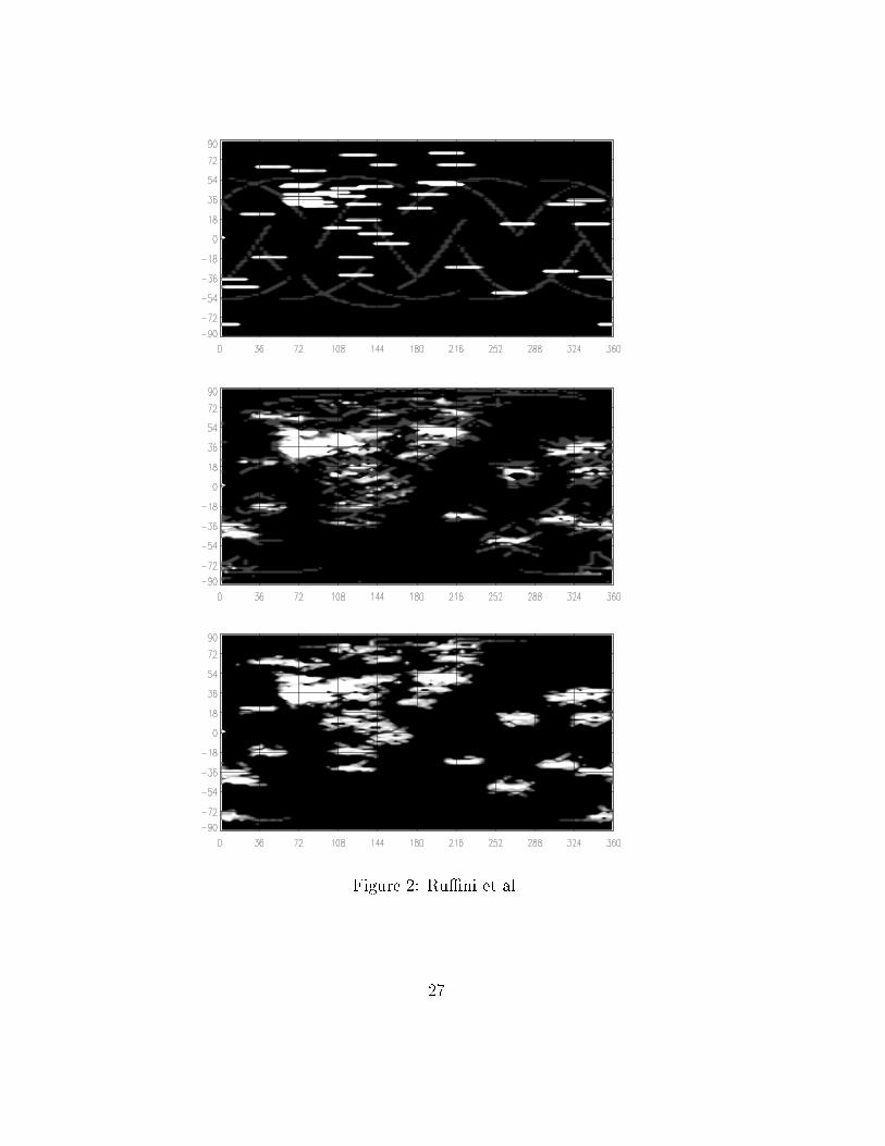
Figure 2: Ru�ni et al.27

Sun-fixed Longitude0 180 360 0 180 360090180

Colatitude

200{350 km 350{500 km180900180900 0 180 360 0 180 360

0 180 360 0 180 360

Figure 3: Ru�ni et al.28

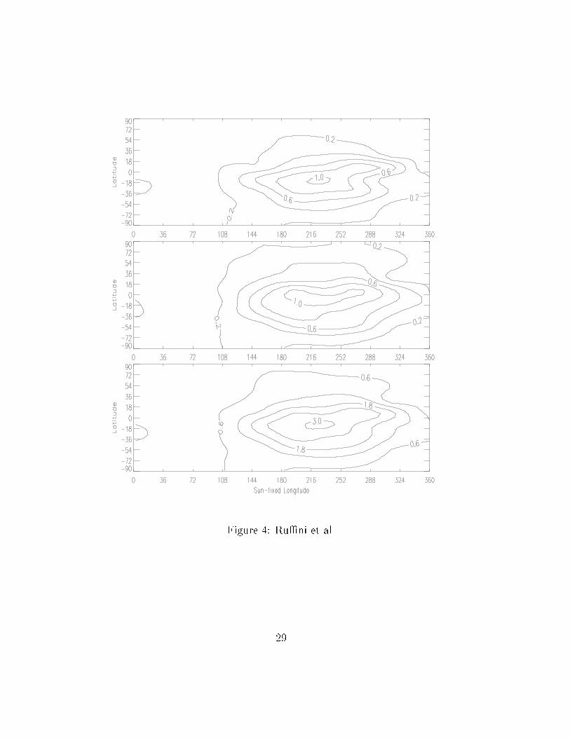
Figure 4: Ru�ni et al.29

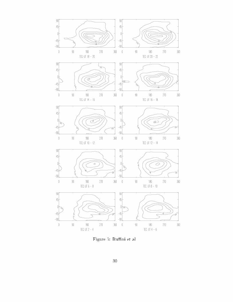
Figure 5: Ru�ni et al.30

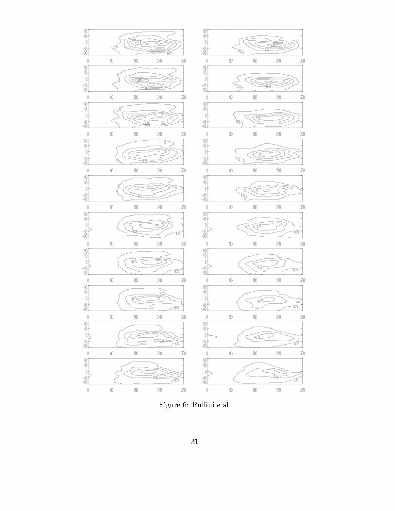
Figure 6: Ru�ni e al.31

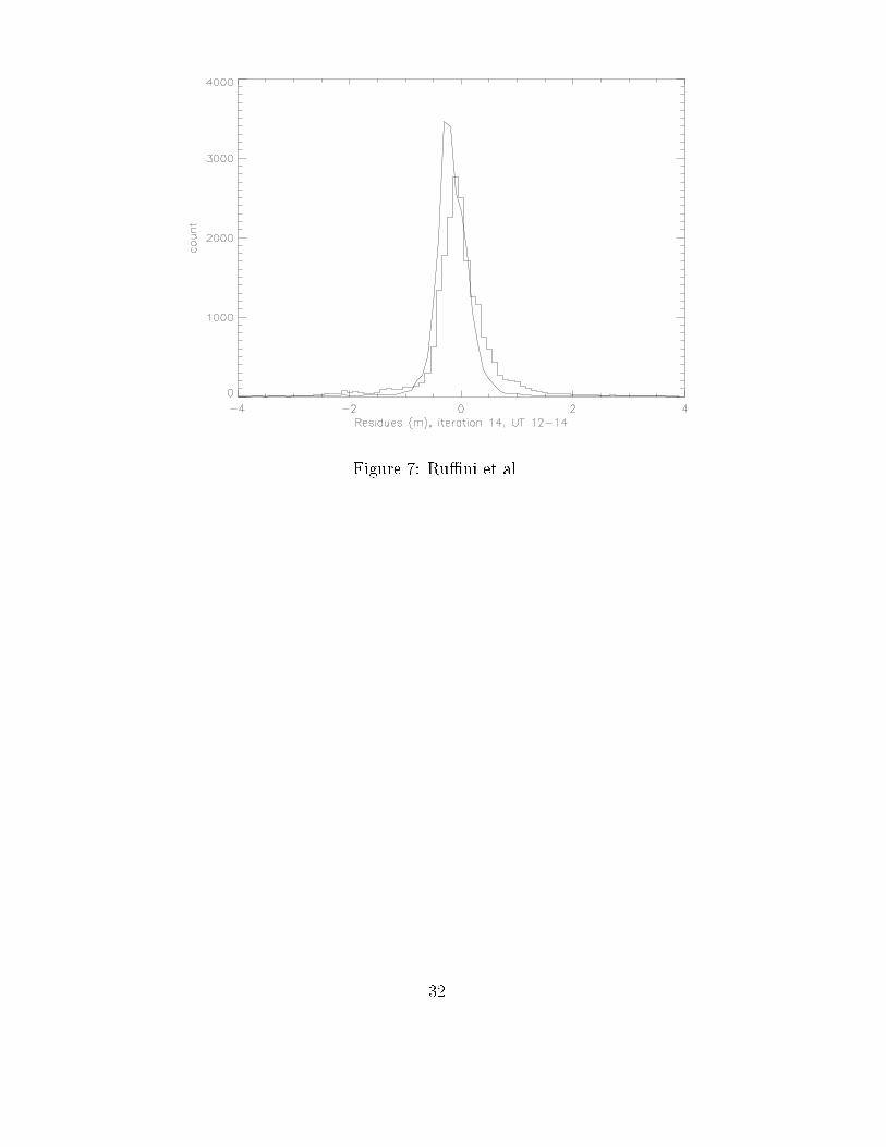
Figure 7: Ru�ni et al.

32

Giulio Ru�ni was born in Barcelona, Spain, in 1966 and is an Italian citizen.He obtained the B.A. degree in Mathematics and in Physics from the Universityof California, Berkeley in 1988, and the M.S. and Ph.D. degrees in Physics fromthe University of California, Davis in 1990 and 1995, respectively. During thesummers of 1990 to 1995 he was a graduate researcher in theoretical physics atthe Los Alamos National Laboratory in New Mexico. He is presently employedat the Institut d'Estudis Espacials de Catalunya in Barcelona (IEEC), Spain, asa researcher in the applications of the GNSS to remote sensing.Alejandro Flores was born in Albacete, Spain,in 1972. He received the B.S.degree in Electrical Engineering from the Polytechnic University of Catalonia,Spain. He joined the IEEC in March, 1996, and has done research in the project\Atmospheric Sounding with GNSS Occultations", sponsored by the EuropeanSpace Agency. He is presently with the Electrical Engineering and ComputerScience department at UC Berkeley, working as a Graduate Student Researcherand pursuing an M.S. degree in Electrical Engineering. His present research isin Hybrid Integrated Circuits, and he has also worked on High TemperatureSuperconductivity.Antonio Rius received the Ph. D. degree in Astrophysics from Barcelona Uni-versity in 1974. From 1975 to 1985 he has been a member of the Technical Sta�at NASA's Deep Space Communications Complex in Madrid, where he has beenresponsible for the radioastronomical activities. Since 1986 he has been with theSpanish Consejo Superior de Investigaciones Cient���cas. Now he is responsiblefor the research group on Earth Observation at the IEEC. His research interestsinclude observational radioastronomy and its applications to Earth Science.

33