GPS Measurements and Its Impact on Geodetic Datum Maintenance By Eng. / ALI JAAFAR DAKHIL FARHAN B.Sc. Building and Construction Department (2002-2003) University of Technology, Baghdad, Iraq Eng. in Ministry of Higher Education and Scientific Research, Al-Qadisiya University, Iraq A Thesis Submitted to the Faculty of Engineering at Mansoura University In Partial Fulfillment of the Requirements for the Degree of Master of Sciencein Public Work Engineering Supervisors 2015 FACULTY OF ENGINEERING MANSOURA UNIVERSITY MANSOURA – EGYPT 2015 Prof.Dr. Eng. MostafaRabah Head of Crustal Movement Lab Department of Geodynamics National Research Institute of Astronomy & Geophysics Helwan, Egypt Prof. Dr. / Mahmoud El-Mewafi Shetiwi Professor of surveying and geodesy, Public Works Department, Faculty of Engineering, Mansoura University Dr. Ahmed Ali Awad Public work Engineering Department Faculty of Engineering, Mansoura University

Welcome message from author
This document is posted to help you gain knowledge. Please leave a comment to let me know what you think about it! Share it to your friends and learn new things together.
Transcript

GPS Measurements and Its Impact on Geodetic Datum Maintenance
By
Eng. / ALI JAAFAR DAKHIL FARHAN
B.Sc. Building and Construction Department (2002-2003)
University of Technology, Baghdad, Iraq Eng. in Ministry of Higher Education and Scientific Research,
Al-Qadisiya University, Iraq
A Thesis Submitted to the Faculty of Engineering at Mansoura University
In Partial Fulfillment of the Requirements for the Degree of
Master of Sciencein Public Work Engineering
Supervisors
2015
FACULTY OF ENGINEERING
MANSOURA UNIVERSITY
MANSOURA – EGYPT
2015
Prof.Dr. Eng. MostafaRabah Head of Crustal Movement Lab
Department of Geodynamics
National Research Institute of
Astronomy & Geophysics
Helwan, Egypt
Prof. Dr. / Mahmoud El-Mewafi Shetiwi
Professor of surveying and geodesy,
Public Works Department,
Faculty of Engineering,
Mansoura University
Dr. Ahmed Ali Awad Public work Engineering
Department Faculty of Engineering, Mansoura
University

GPS Measurements And Its Impact on Geodetic Datum Maintenance
By
Eng. / ALI JAAFAR DAKHIL FARHAN
B.Sc. Building and Construction Department (2002-2003)
University of Technology, Baghdad, Iraq Eng. in Ministry of Higher Education and Scientific Research,
Al-Qadisiya University, Iraq
A Thesis Submitted to the Faculty of Engineering at Mansoura University
In Partial Fulfillment of the Requirements for the Degree of
Master of Sciencein Public Work Engineering
Approved by the Examining Committee:
Prof. Dr. Ali Abdel Azim Thoeilb External Examiner
Prof. Dr. Zaki Mohamed Zedan Internal Examiner
Prof. Dr. Eng. Mahmoud EL-Mewafi, Thesis Main Advisor...
Public work Engineering Department, Faculty of Engineering, MANSOURA University
Prof.Dr. Eng. MostafaRabah, Head of Crustal Movement Lab
Department of Geodynamics National Research Institute of Astronomy & Geophysics Helwan
FACULTY OF ENGINEERING
MANSOURA UNIVERSITY MANSOURA – EGYPT
2015
FACULTY OF ENGINEERING
MANSOURA UNIVERSITY
MANSOURA – EGYPT
2015

قرآ ية
(سورة البقرة 23)

Dedication
ƯƯƯƯƯƯƯƯƯƯƯƯƯƯƯƯƯƯƯƯƯƯƯƯƯƯƯƯƯƯƯƯƯƯƯ
The spirit of the deceased
&&My Son Jaafar&&
&&&&&
Will never forget you
Ali Jaafar Dakhil
2015

IN THE NAME OF
ALLAH
THE BENEFICENT, THE MERCIFUL
"Praise to Allah, Who guided us to this;
And
in no way could we have been guided,
unless Allah has guided us"
(AL A'raf 43)

Acknowledgements
I
Acknowledgements
The author wishes to express his most sincere gratitude and thanks to Prof. Dr.
Mahmoud El-Mewafi, The head of Public Works Department, Faculty of
Engineering, Mansoura University, for his supervision, valuable guidance, enormous help,
and discussion throughout this study.
I would like to give my cordial thanks and respect to Prof. Dr. Mostafa Rabah, Head
of Crustal Movement Lab Department of Geodynamics National Research Institute of Astronomy
& Geophysics
And my cordial thanks and respect to Dr. Ahmed Ali Awad, Public work Engineering
Department Faculty of Engineering, Mansoura University
As I like to express my grateful thanks to the Ministryof Higher Education and
Scientific Research in Iraq for their role and support me in accomplishing this thesis.
And finally, "not least" I extend my thanks and gratitude to the Deanship of the Faculty of
Engineering, Mansoura University, represented by the person of Mr. Dean Prof. Dr.
Zaki Mohamed Zedan.
Ali Jaafar Dakhil
2015

Abstract
II
Abstract:
One of the fundamental goals of geodesy is to precisely define positions of
points on the surface of the Earth, so it is necessary to establish a well-defined geodetic
datum for geodetic measurements and positioning computations. Recently, a set of the
coordinates established by using Global Positioning System ( GPS ) and referred to
an international terrestrial reference frame could be used as a three-dimensional
geocentric reference system for a country. Based on this modern concept, in 1992, the
Egyptian Survey Authority (ESA) established two networks. The first net is called High
Accuracy Reference Network (HARN) and consisted of 30 stations, 200 km spacing.
The second network was established to cover the cultivated areas (Nile Valley and
Delta) so it is called the National Agricultural Cadastral Network (NACN) with spacing
30 to 40 km. To transfer the International Terrestrial Reference Frame to the HARN,
the HARN was connected with four International GNSS Service (IGS) stations,
namely MATE (Italy), KIT3 (Uzbekistan), HART (South Africa) andMASP in (Canary
Island). The results of analyzing both of HARN and NACN were defined in
International Terrestrial Reference Frame (ITRF1994) epoch 1996.The
processing results were 1:10,000,000 (Order A) for HARN and 1:1,000,000 (Order B)
for NACN relative network accuracy standard between stations defined in ITRF1994
Epoch 1996. The following studies were done by the current research:
To evaluate the specified part, the available, of HARN & NACN stations in the
Nile Delta and surroundings andto see for what extent can Precise Point
Positioning (PPP) be an alternative for the differential GNSS techniques, a
Processing was done by Canadian Spatial Reference System (CSRS-PPP) Service
based on utilizing Precise Point Positioning (PPP) and Trimble Business Center
(TBC). Additionally, seven test points were processed by Trimble Business Center
“TBC” Software, the product of Trimble, with considering the PPP solution of
PHLW as a reference station for the processing. Based upon the computed
results,one can easily see that the quality of PPP solution compared with the
Differential Global Positioning System (DGPS) solution,in spite of the processed
baselines are exceed several tens of kilometers to 120 km, PPP shows a good
harmony with the DGPS in mm level.
To see how the PPP can be used in updating the ITRF of the IGS points, several
IGS stations were computed by PPP solution in ITRF2008 at Epoch 2015.274 and
the results were compared with the published IGS ITRF2008 at the same Epoch.

Abstract
III
The differences between two solutions were: the absolute value of the maximum
differences does not exceed 17mm for the Y component of NicoStation, Cyprus,
while does not exceed few mm for the other stations.
The results confirm the usability of PPP in updating the frame.
To evaluate the IGS stations that were used in transferring the ITRF1994 to
HARN, by transferring their published ITRF2008 Epoch2015.422 coordinates
values and the related transformation parameter to ITRF1994 Epoch1996 and
compares the transferred values by the reported values of (Scott ,1997).We used
only in the previous processing the published values and models as specified by
IGS.The computed differences shows a tolerance ranged between -8.6 cm to
14.6 cm. The reasons behind these differences are mostly returning to that were
used in realizing the ITRF94 that leads to sub-optimal stations distribution and
small discontinuities between IGS realizations of ITRF, as clarified by (Ferland
and Kouba, 1996).
To see for what extent can the PPP be an alternative for the differential
techniques in updating the geodetic frame and to study its impact in analyzing
the geodetic applications that need an ultimate accuracy like the National HARN
of Egypt, a critical example is given to demonstrate this study. The example is
concerned with analyzing a part of Egypt HARN and NACN (National
Agriculture Cadastre) Networks that is located in and around Nile
Delta.Transferring the values of HARN & NACN networks that were defined in
ITRF2008 epoch 2015.274 to the original ITRF frame of HARN, namely
ITRF1994 epoch 1996 and compare the resulted values with the original
coordinate‟s values given by Scott (1997) exploiting the published 14
transformation parameters between different ITRF‟s Frames by IGS. The
differences were ranged in X-component from 34 to 37 cm, except 0Z18(66cm)
that was partially destroyed, and Y-component ranged from -8 cm to -11 cm and
for Z-component, the differences were ranged between -7 cm and -8 cm, except
0Z18.
One can say that PPP is the most feasible factor in performing datum
maintenance by time and cost.
The Egyptian HARN & NACN Networks need to update their frame, to be the
most recent one either by PPP or traditional approach.

IV
Contents
Subject Page
Acknowledgements……………………………………………………………………………. I
Abstract………………………………………………………………………………………… II
Table of Contents……………………………………………………………………………… IV
List of Figures………………………………………………………………………………….. VI
List of Tables…………………………………………………………………………………... VII
Chapter 1 – Introduction
1.1.Introduction……………………………………………………………………………….. 1
1.2.Statement of the Problem…………………………………………………………………. 2
1.3.Objectives of the Thesis…………………………………………………………………… 6
1.4.Scope of Thesis 7
Chapter 2 – Introduction to GPS Measurements
2.1. GPS Overview…………………………………………………………………………….. 8
2.2. The Precise Point Positioning “PPP” …………………………………………………….. 26
Chapter 3 – Introduction to Geodetic Datums
3.1. Introduction to Geodetic Datums…………………………………………………………. 43
3.2. Modern Geodesy and ITRS/ITRF………………………………………………………… 45
3.3. World Geodtic System (WGS84) ………………………………………………………… 52
3.4. The Datum Problem………………………………………………………………………. 53

V
Subject Page
3.5. Kinematic Transformation Parameters Using Rigid Plate Rotation Model………...…….. 57
Chapter 4 – Geodetic Control Networks
4.1. Network Establishment and Control Based on Hierarchial Orders……………………….. 61
4.2. Requirements for the Position of Control Points………………………………………….. 62
4.3. Erection of Survey Marks and Monument Setting………………………………………... 64
4.4. The Egyptian Geodtic Control Network…………………………………………………... 66
4.5. GPS Control Network……………………………………………………………………... 67
4.6. Marking the Position of the GPS Control Point…………………………………………... 70
4.7. Introduction to Network Adjustment……………………………………………………. 75
4.8. GPS Network Adjustments Procedures…………………………………………………. 77
4.9. Adjustment of GPS Network Models……………………………………………………. 81
4.10. Continuously Operating Reference System…………………………………………….. 83
Chapter 5 – Experimental Results & Evaluation
5.1. Transformation Parameters Terrestrial Reference Systems “TRS” …………………….. 90
5.2. PPP Solution……………………………………………………………………………... 93
5.3. The Evaluation Study……………………………………………………………………. 97
Chapter 6 – Conclusions and Recommendations
6.1. Conclusions………………………………………………………………………………
6.2. Recommendation………………………………………………………………………… 111
References…………………………………………………………………………………….. 112
107

VII
List of Figures
Caption
Figure No. Page
1.1.The Egyptian First Order Triangulation Networks ………………………………………. 3
1.2.The HARN & NACN Networks ………………………………………………… 4
1.3. Connecting parts of Egyptian HARN with four stations of IGS…………………………
2.1 The GPS satellite constellation ………………………………………………………10
5
2.2. The single-difference technique ………………………………………………………….. 16
2.3. The double-difference technique ………………………………………………………..... 18
2.4. The triple-difference technique…………………………………………………................ 19
3.1. Local datum with best fit ellipsoid ……………………………………………………….. 44
3.2. Geocentric datum with ellipsoid that is a best fit to the world …………………………… 45
3-3.Conventional Celestial System (CRS)……………………………………………………. 48
3-4.Conventional Terrestrial System (CTS)………………………………………………….. 49
3-5.International Terrestrial Reference System (ITRS)………………………………………. 49
3-6. World Geodetic System 1984 (WGS84)……… …………………………………………. 53
3-7.Rigid Plate Rotation ……………………………………………………..……………….. 58
4.1. Monumentation of the first- and second-order trig points………………………………… 65
4.2.The Egyptian First Order Triangulation Networks ………………………………………. 71
4.3. GPS survey network.……………………………………. …………………………. 83
4.4. The Monumentation of one Core Station ………………………………………... 84

VII
Caption
Figure No. Page
5.1 The Africa tectonics sub-plates …………………….……………………. 92
5.2 The location of the used part of Egypt HARN & NACN ………………. 99
5.3 Station set (13) used for IGS Realization of ITRF 92-93-94 …………… 103

VIII
List of Tables
Caption
Table No. Page
1. The offset in Helwan coordinate values by using the static datum…………………………. 6
2.1. The characteristics of the used linear combinations………………………………………. 21
4-2.Differences between reference systems…………………………………………………... 50
4.1. Accuracy and density of GPS control networks…………………………………………... 70
5.1. The Cartesian angular Velocity of Nubian Plate………………………………….............. 93
5.2. ITRF2008 STATION POSITIONS AT EPOCH 2005.0 AND VELOCITIES.................... 95
5.3. DATA SET EXPRESSED IN ITRF2008 FRAME
STATION POSITIONS AND VELOCITIES AT EPOCH 2015/04/10……………………….
95
5.4.the updated positioning for four IGS stations defined in ITRF2008 epoch 2015.274 by
IGS & PPP…………………..…………………..…………………..…………………..……...
96
5.5 The differences between DGPS & PPP solutions for the observed Stations 97
5.6. The coordinates of chosen points of the HARN and NACN Networks…………………... 98
5.7. The Part of HARN & NACN network updated in ITRF2000……………………………. 99
5.8. Transformation parameters Between ITRF2008 Epoch 2005 to ITRF 1994 Epoch 2000... 100
5.9. The coordinate values of the IGS four stations in ITRF1994, Epoch 1996 and the
published coordinate values for the nominated IGS stations in ITRF2008
Epoch2005……………………………………………………..…………………………….....
102
5.10 .The transferred coordinate values of the four stations to ITRF1994 Epoch2000……….. 102

XI
Caption
Table No.
Page
5.11. The values of the published coordinate values of the four IGS stations & the reported
values by (Scott, 1997) in ITRF1994 Epoch1996……………………………………………...
102
5.12. The differences between the published coordinate values of the four IGS stations & the
reported values by (Scott, 1997) in ITRF1994 Epoch1996…………………………………….
103
5.13. The Results of Transformation the HARN to ITRF 1994 Epoch 1997…...……………... 104
5.14. The computed velocities and the transferred coordinate values to ITRF 94 Epoch 96 of
the specified part of the Egyptian HARN………………………………………………………
105
5.15. The values of the computed PPP HARN transferred to ITRF 94 Epoch 96 and the given
values at the same epoch as computed by Scott (1997)………...……..… ……………………
105
5.16. The Difference between the computed PPP HARN transferred to ITRF 94 Epoch 96
and the given values at the same epoch as computed by Scott (1997)…………………………
106

List of Abbreviations
AFREF African Reference Frame
APC Antenna Phase Center
APREF Asia-Pacific Reference Frame
ARP Antenna Reference Point
C/A Code Coarse Acquisition
CEP Conventional Ephemeris pole
CIS Conventional Inertial System
CORS Continuously Operating Reference Station CRF Celestial Reference Frame
CRS Celestial Reference System
CTP Conventional Terrestrial Pole
CTS Coordinated Terrestrial System
DGPS Differential Global Positioning System
DMA United States Defence Mapping Agency
DoD US Department of Defense
ECEF Earth-Centered, Earth-Fixed
ECI Earth centered inertial
EPGN Egyptian Permanent GPS Network
ESA Egypt Survey Authority
ETRF European Terrestrial Reference Frame
Finmap Finnish Project in the Eastern Desert
GNSS Global Navigation Satellite System
GPS Global Positioning System
HARN High Accuracy Reference Network
IAG International Association of Geodesy
IAU International Astronomical Union
ICRS International Celestial Reference System ICRS International Celestial Reference System
IERS International Earth Rotation Service
IGS International GNSS Service
ITRF International Terestial Reference Frame
ITRS International Terrestrial Reference System
JPL NASA's Jet Propulsion Laboratory
LADGPS Local Area Global Positioning System
NACN National Agricultural Cadastral Network
NAD83 North American Datum 1983
NGIA National Geospatial -Intelligence Agency

NNR no-net-rotation
NRCan Natural Resources Canada
NRIAG National Research Institute for Astronomy and Geophysics
PMM Plate Motion Model
PPP Precise Point Positioning
PPS Precise Positioning Service
PRN Pseudo Random Noise
RTK Real-time, kinematic
SA Selective Availability
SIRGAS Sistema de Referencia Geocentrico para las America
SLR Satellite Laser Ranging
SNR Signal-to-Noise Ratio
SPS Standard Positioning Service
SRI Survey Research Institute
TBC Trimble Business Center
TRS Terrestrial Reference System
UNB University of New Brunswick
UTM Universal Transverse Mercator
VLBI Very Long Baseline Interferometry
WADGPS Wide Area Global Positioning System
WGS84 World Geodetic System of 1984

Chapter 1 - Introduction
Page 1
1.1. Introduction
In space geodetic positioning, where the observation techniques provide
absolute positions with respect to a consistent terrestrial reference frame, the
corresponding precise definition and realization of terrestrial and inertial reference
systems is of fundamental importance. Thanks to significant improvements in receiver
technology, to extension and densification of the global tracking network along with
more accurate determination of positions and velocities of the tracking stations and to
dramatically improved satellite orbits, GPS is today approaching 0.1 ppm precision for
longer baselines and it can be considered to be the main global geodetic positioning
system providing nearly instantaneous three-dimensional position at the cm accuracy
level. One of the fundamental goals of geodesy is to precisely define positions of points
on the surface of the Earth, so it is necessary to establish a well-defined geodetic datum
for geodetic measurements and positioning computations. Recently, a set of the
coordinates established by using GPS and referred to an international terrestrial
reference frame could be used as a three-dimensional geocentric reference system for a
country (Abidin, H. ,1993a).
In the classical sense, a geodetic datum is a reference surface, generally an
ellipsoid of revolution of adopted size and shape, with origin, orientation, and scale
defined by a geocentric terrestrial frame. Once an ellipsoid is selected, coordinates of a
point in space can be given in Cartesian or geodetic (curvilinear) coordinates (geodetic
longitude, latitude, and ellipsoid height).
Two types of geodetic datum can be defined namely a static and kinematic
geodetic datum. A static datum is thought of as a traditional geodetic datum where all
sites are assumed to have coordinates which are fixed or unchanging with time. This is
an incorrect assumption since the surface of the earth is constantly changing because of
tectonic motion. Static datum does not incorporate the effects of plate tectonics and
deformation events. Coordinates of static datum are fixed at a reference epoch and
slowly go out of the date, need to change periodically which is disruptive.
Datum's can either become fully kinematic (dynamic), or semi-kinematic. A
deformation model can be adopted to enable ITRF positions to be transformed into a
static or semi-kinematic system at the moment of position acquisition so that users do

Chapter 1 Introduction
Page 1
not see coordinate changes due to global plate motions. GNSS devices which use ITRF
or closely aligned systems position users in agreement with the underlying kinematic
frame, however, in practice there are a number of very significant drawbacks to a
kinematic datum. Surveys undertaken at different epochs cannot be combined or
integrated unless a deformation model is applied rigorously, or is embedded within the
data, and the data are correctly time-tagged. On the other hand, Semi–Kinematic datum
incorporates a deformation model to manage changes (plate tectonics and deformation
events). Coordinates fixed at a reference epoch, so the change to coordinates is
minimized. Many countries and regions which straddle major plate boundaries have
adopted a semi-kinematic (or semi-dynamic) geodetic datum in order to prevent
degradation of the datum as a function of time due to ongoing crustal deformation that
is occurring within the country.
High precision GNSS positioning and navigation is very rapidly highlighting the
disparity between global kinematic reference frames such as ITRF and WGS84, and
traditional static geodetic datum. The disparity is brought about by the increasingly
widespread use of PPP and the sensitivity of these techniques to deformation of the
Earth due to plate tectonics. In order for precision GNSS techniques to continue to
deliver temporally stable coordinates within a localized reference frame.
1.2. Statement of the Problem
Between 1853 and 1859 a survey of Egypt was made but did not depend on a
triangulation scheme (Shaker A.A.,1982). Later, many attempts were made for
constructing a geodetic triangulation, but they were not of higher order. In 1874 a
number of expeditions were led by British scientists to various European colonies in
Africa and the Indian Ocean in order to simultaneously observe the transit of Venus for
the purpose of precisely determining differences in longitude. Locations included
Mauritius, Rodrigues, Réunion, St. Paul and Egypt. Helwan Observatory situated on Az
Zahra Hill in the Al-Moqattam Hills, South of Cairo was utilized for the observations,
and the station was termed “F1” where: Φo = 30º 01‟ 42.8591” N, Λo = 31º 16‟ 33.6”
East of Greenwich, the initial La Place azimuth being measured from Station O1
(Helwân) to Station B1 (Saccara), αo = 72º 42‟ 01.20” from South, and Ho = 204.3 m,
based on mean sea-level at Alexandria. This is considered the origin of the “Old Egypt
Datum of 1907” (Clifford J. Mugnier ,2008).

Chapter 1 Introduction
Page 2
It just so happens that M. Sheppard, director general of the Survey of Egypt,
reported (in French) to the Secretary General of the Geodesy Section of the
International Union of Geodesy and Geophysics that the initial geodetic work
performed in Egypt was computed on the Clarke 1866 ellipsoid where: “a, demi-grande
axe equatorial =6.378.206m (sic), α = 1/295 (sic).” Sheppard went on to say that all
cultivated lands in the Nile Valley that were based on 2nd and 3rd order triangulations
(for cadastral applications) initially used this ellipsoid, but that a later controlling chain
of triangulation spanning the length of the Nile Valley was computed with the later
adopted Helmert (1906) ellipsoid where a, = 6.378.200 m, 1/f = 1/298.3. Everything
was later re-calculated on the Helmert ellipsoid and also on the International 1924
ellipsoid where a = 6,378, 388 m, 1/f = 297 (Bulletin géodésique, 1925) , (Clifford J.
Mugnier , 2008).
In 1907 it became possible to begin a new work for establishing a geodetic
triangulation frame for Egypt, which is considered to be the first national network to be
established in Africa (Moritz, 1981). From the cost point of view, it was decided to
carry out the network along the Nile Valley only (Shaker, 1982). The main reason to
carry it out was to fix, with a great possible accuracy, fundamental control-stations to be
a base for the cadastral survey and national mapping of the country. Egyptian network
was extended to Sudan and other African nations. The first order geodetic horizontal
control network of Egypt contains two main networks, Network (1) and Network (2),
(Cole, J., 1944). Figure (1.1) shows the first order triangulation networks.
In 1930, after a re-adjustment of the classical network, the New Egypt Datum of
1930 was published, also referenced to the Helmert1906 ellipsoid. The common
abbreviation for the new datum is “EG30.” This remains the current classical system
used in Egypt for civilian mapping purposes.
In 1992, an Egypt Survey Authority (ESA) steering committee developed a plan
for the creation of new datum for Egypt, with the following approach (Scott, 1997):
First, observe approximately 30 stations at approximately 200 km interval,
covering all of Egypt, creating a High Accuracy Reference Network (HARN).
Both high absolute and relative accuracies are required for these stations.

Chapter 1 Introduction
Page 3
Second, establishing the Notational Agricultural Cadastral Network (NACN)
relative to these 30 stations, covering the green area of Egypt (Nile Valley and
the Delta) at 30-40 km intervals. This station spacing was selected to allow for
further densification with single frequency receivers, see figure (1.2).
Third, densify this network at a station spacing of approximately 5 km for use as
cadastral control at the governorate level.
Finally, replace the existing Egyptian Mercator grid with a new modified UTM
coordinate system.
Each station was observed for six sessions, every session was 6 hours with 30
seconds epoch interval. The observation time was planned to produce 1:10,000,000
(Order A) for HARN and 1:1,000,000 (Order B) for NACN relative network accuracy
standard between stations. The results of analyzing both of them were defined in
ITRF1994 epoch 1996.
Figure (1.1): The Egyptian First Order Triangulation Networks.

Chapter 1 Introduction
Page 4
Figure (1.2.): The HARN & NACN Networks
The ITRF1994 was transferred to Egypt‟s HARN network by connecting it with four
IGS stations, namely MATE (Italy), KIT3 (Uzbekistan), HART (South Africa) and
MASP in (Canary Island), see figure (1.3). Each HARN‟s station was observed for six
sessions, every session was 6 hours with 30 seconds epoch interval. The observation
time was planned to produce 1:10,000,000 (Order A) for HARN and 1:1,000,000 (Order
B) for NACN relative network accuracy standard between stations. The results of
analyzing both of them were defined in ITRF1994 epoch 1996.

Chapter 1 Introduction
Page 5
Figure (1.3): Connecting parts of Egyptian HARN with four stations of IGS
(Rabah et. al., 2015) proofed the drawback of the currently used Egypt static
datum, namely ITRF1994 Epoch 1996, based on GPS Observation Campaign 1996.
Because Helwan is considered the only station that was used in updating the ITRF2008
geodetic frame, the values of Helwan coordinates at any Epoch can be computed by
(http://itrf.ensg.ign.fr/site_info_and_select/solutions_extraction.php). So, Helwan
coordinate values was computed by IGS computing center Helwan IGS Station with in
ITRF2008 Epoch2015.274. Helwan was transferred by the published transformation
parameters, computed by (http://itrf.ign.fr/trans_para.php) to ITRF1994 Epoch 1996 The
related Reference Frame coordinate values, related velocity parameters and the
differences are tabulated in table (1.1). As it is indicated in the table, the differences
between Helwan coordinate values defined in ITRF2008 Epoch 2015 and the values
defined in ITRF1994 Epoch 1996 are: -41.8 cm for X component, 26 cm for Y
component and 31.6 cm for Z component. These discrepancies exceed any accuracy
requirements needed by any control works.

Chapter 1 Introduction
Page 6
Table (1.1.): The offset in Helwan coordinate values by using the static datum
Reference Frame HELWAN
IGS- ITRF2008 Epoch2015.274 4728141.098 2879662.549 3157147.092
Published ITRF2008 Epoch2005 4728141.309 2879662.406 3157146.932
Published Vx, Vy, Vz (m/year) -0.0211 0.0143 0.016
ITRF1994Epoch1996 4728141.516 2879662.289 3157146.776
Differences -0.418 0.260 0.316
1.3 Objectives of the Thesis
To study the situation of the HARN & NACN Network after passing more than
20 years, a check for existing HARN monuments in and around Delta. To
evaluate the PPP and answering wither PPP can be used as an alternative for
DGPS in geodetic Control Networks. Several (PPP) tests on several IGS station
were performed.
To see the quality of the HARN and NACN networks solution, the selected GPS
stations were estimated in its International Terrestrial Reference Frame (ITRF)
at the day of the observing campaign and site velocities given by the
International Earth Rotation Service (IERS) and then transformed to the original
processed ITRF datum, namely ITRF1994, epoch 1996.
To perform the required transformation processing, PPP GPS processing
techniques was utilized in the transformation process as well as a three
parameters kinematic rigid plate model.
To push Responsible authorities for maintenance of networks that represent the
references (datum)
To push the inevitability of updating of HARN and NACN according to the
latest frame by taking a modern observation to them and analyze it by PPP
To see the impact of tectonic and evaluate the results in terms of the required
level of accuracy.

Chapter 1 Introduction
Page 7
1.4 . Scope of Thesis
In addition to this chapter, the thesis consists of four chapters as follows:
1.4.1 Chapter Two: Introduction to GPS Measurements. This chapter contains GPS
Overviewand the principle of operation, segments of the system, error of
system, GPS Observation Equations, Relative Positioning Modes, The Precise
Point Positioning "PPP", Mathematical Model of Precise Point Positioning, and
adjustment of GPS processing.
1.4.2 ChapterThree: Introduction to Geodetic Datums, This chapter discusses the
different types of Geodetic datums and their relation to Modern Geodesy and
ITRS/ITRF, World Geodetic System (WGS84). It also explains the datum
problem, Kinematic Transformation Parameters Using Rigid Plate Rotation
Models.
1.4.3 ChapterFour: Introduction to Geodetic Control Networks, This chapter deals
with Geodetic Control Networks, Geodetic Horizontal Network Standards,
GPS Networks, Control Survey Requirements, Network Design, and
Introduction to Network Adjustments.
1.4.4 ChapterFive: This chapter explains how data were collected and analyzedand
as well as discussing and evaluating of the obtained results ,
1.4.5 Chapter six::Conclusions and Recommendations: Thischapter contains the
main conclusions that were derived from the research work and
recommendations for the future study.

Chapter 2 Introduction to GPS Measurements
Page 8
Chapter 2
Introduction to GPS Measurements
2.1 . GPS Overview
The Global Positioning System (GPS) is an all-weather, space-based navigation
system. This system is development by the US Department of Defense (DoD) to satisfy
the requirements of the military forces to accurately determine their position, velocity
and time in a common reference system, anywhere on or near the earth on a continuous
basis.
2.1.1 The principle of operation
The GPS satellites transmit radio signals giving the position of each satellite and
the time of transmitting the signal. These signals can be received on the earth with a
receiver. The distance between a satellite and the receiver can be computed by
multiplying the speed of light with difference between the times that the signal left the
satellite and the time that it arrives at the receiver. If the distances to four or more
satellites are measured simultaneously, then a three dimensional position on the earth
can be determined. GPS positioning capability is provided at no cost to civilian and
commercial users world-wide at an accuracy level of 100 meters. This accuracy level is
known as the Standard Positioning Service (SPS). The US military and its allies, and
other authorized users, receive a specified accuracy level of 21 meters, known as the
Precise Positioning Service (PPS). The full accuracy capability of GPS is denied to
users of the SPS through a process known as Selective Availability (SA). This
purposeful degradation in GPS accuracy is accomplished by intentionally varying the
precise time of the clocks on board the satellites and by providing incorrect orbital
positioning data in the GPS navigation message. SA is normally set to a level that will
provide 100 meter positioning accuracy to users of the Standard Positioning Service. In
practice, several additional sources of error other than SA can affect the accuracy of a
GPS-derived position. They include unintentional clock and ephemeris errors, errors
due to atmospheric delays, multipath errors, errors due to receiver noise, and errors due
to poor satellite geometry (Hofmann-Wellenhof, 1994).

Chapter 2 Introduction to GPS Measurements
Page 9
Differential GPS (DGPS) is the most widely used method of GPS augmentation
and significantly improves the positioning accuracy. DGPS makes use of GPS reference
stations at locations which have been geodetically surveyed and so are known with a
very high accuracy. These stations observe GPS signals in real time and compare their
measurements to the ranges expected to be observed at the fixed positions of the
stations. The differences between the observed and the predicted ranges are used to
compute the corrections to GPS parameters like error sources, resultant positions, or
observations. These differential corrections are then transmitted to GPS users, who
apply the corrections to their received GPS signals or the computed position. Depending
on the user application, DGPS reference stations can be permanent, elaborate
installations, or they can be small, mobile GPS receivers that can be moved to various
well surveyed locations. The equipment used to broadcast differential corrections, the
type of radio data link used, and the size of the geographic area covered by the DGPS
system also vary greatly with the application. Differential systems can be Local Area
(LADGPS) or Wide Area (WADGPS). The LADGPS broadcasts differential
corrections over a limited geographic area, while the WADGPS can cover a continent or
more. For civil applications, DGPS can provide sub-meter accuracy (Leick, 1995).
2.1.2 The segments of the system
The GPS system consists of three segments, the space segment consisting of
satellites which broadcast signals, the control segment managing the whole system, and
the user segment including the all types of receivers which receive the satellite signals.
2.1.2.1 Space Segment
The Space segment of the system consists of the GPS satellites. These satellites
send radio signals from space. The GPS operational constellation consists of 24
satellites: 21 navigational satellites and 3 active spares orbit the earth in 12 hour orbits
as shown in figure

Chapter 2 Introduction to GPS Measurements
Page 10
Figure (2.1.): The GPS satellite constellation.
These orbits repeat the same ground track (as the earth turns beneath them) once
each day. The orbit altitude is such that the satellites repeat the same track and
configuration over any point approximately every 24 hours (4 minutes earlier each day).
This is accomplished by satellites in nearly circular orbit with an altitude of about
20200 km above the earth. There are six orbital planes (with nominally four satellites in
each), equally spaced (60 degrees apart), and inclined at about fifty-five degrees with
respect to the equatorial plane. This constellation provides the user with between five
and eight satellites visible from any point on the earth. The GPS satellites provide a
platform for radio transceivers, atomic clocks, computers and various equipment used
for positioning requirements. The equipment of the satellites allows the user to operate a
receiver to measure simultaneously distances to more than three satellites. Each satellite
broadcasts a message which allows the user to determine the spatial position of the
satellite (US Department of Defense, 1996).
The satellites in the GPS constellation are arranged into six equally-spaced
orbital planes surrounding the Earth. Each plane contains four "slots" occupied by
baseline satellites. This 24-slot arrangement ensures users can view at least four
satellites from virtually any point on the planet.The Air Force normally flies more than
24 GPS satellites to maintain coverage whenever the baseline satellites are serviced or
decommissioned. The extra satellites may increase GPS performance but are not
considered part of the core constellation.

Chapter 2 Introduction to GPS Measurements
Page 11
In June 2011, the Air Force successfully completed a GPS constellation
expansion known as the "Expandable 24" configuration. Three of the 24 slots were
expanded, and six satellites were repositioned, so that three of the extra satellites
became part of the constellation baseline. As a result, GPS now effectively operates as a
27-slot constellation with improved coverage in most parts of the
world(Offi.US.Gov.info.GPS, 2015).
2.1.2.2 Control Segment
The Control Segment consists of a system of tracking stations located around the
world. The control segment monitors the functioning of the satellites and uploads
orbital, clock correction, and auxiliary data into the satellite memories. This segment
consists of two main parts, GPS Master Control, and Monitor Network. The Master
Control facility is located at Falcon Air Force Base in Colorado. The monitor stations
measure signals from the satellites which are incorporated into orbital models for each
satellite. The models compute precise orbital data (ephemeris) and satellite clock
corrections for each satellite. The Master Control station uploads ephemeris and clock
data to the satellites. The satellites then send subsets of the orbital ephemeris data to
GPS receivers over radio signals.
2.1.2.3 User Segment
The GPS User Segment consists of all the GPS receivers and the user
community. GPS receivers convert satellite signals into position, velocity, and time
estimates. Four satellites are required to compute the four dimensions of position (X, Y,
Z) and time. GPS receivers are used for navigation, positioning, time dissemination, and
other research. Navigation in three dimensions is the primary function of GPS.
Navigation receivers are made for aircraft, ships, ground vehicles, and for hand carrying
by individuals. Precise positioning is possible using GPS receivers at reference
locations providing corrections and relative positioning data for remote receivers.
Surveying, geodetic control, and plate tectonic studies are examples. Time and
frequency dissemination, based on the precise clocks on board the satellites and
controlled by the monitor stations, are another use for GPS. Astronomical observatories,
telecommunication facilities, and laboratory standards can be set to precise time signals
or controlled to accurate frequencies by special purpose GPS receivers.

Chapter 2 Introduction to GPS Measurements
Page 12
2.1.3 The satellite signals
The satellite transmits two microwave carrier signals. These signals are L1
frequency (1575.42 MHz) and L2 frequency (1227.60 MHz). The C/A Code (Coarse
Acquisition) modulates the L1 carrier phase. The C/A code is a repeating 1 MHz
Pseudo Random Noise (PRN) Code. This noise-like code modulates the L1 carrier
signal, "spreading" the spectrum over a 1 MHz bandwidth. The C/A code repeats every
1023 bits (one millisecond). There is a different C/A code PRN for each satellite. GPS
satellites are often identified by their PRN number, the unique identifier for each
pseudo-random-noise code. The C/A code that modulates the L1 carrier is the basis for
the civil SPS. The P-Code (Precise) modulates both the L1 and L2 carrier phases. The
P-Code is a very long (seven days) 10 MHz PRN code. In the Anti-Spoofing (AS) mode
of operation, the P-Code is encrypted into the Y-Code. The encrypted Y-Code requires
a classified AS module for each receiver channel and is for use only by authorized
users with cryptographic keys. The P (Y)-Code is the basis for the PPS. The Navigation
Message also modulates the L1-C/A code signal. The Navigation Message is a 50 Hz
signal consisting of data bits that describe the GPS satellite orbits, clock corrections,
and other system parameters. The GPS navigation message consists of time-tagged data
bits marking the time of transmission of each sub frame at the time they are transmitted
by the satellite. A data bit frame consists of 1500 bits divided into five 300-bit sub
frames. A data frame is transmitted every thirty seconds. Three six-second sub frames
contain orbital and clock data. Satellite clock corrections are sent in sub frame one and
precise satellite orbital data sets (ephemeris data parameters) for the transmitting
satellite are sent in sub frames two and three. Sub frames four and five are used to
transmit different pages of system data. An entire set of twenty-five frames (125 sub
frames) makes up the complete Navigation Message that is sent over a 12.5 minute
period. Data frames (1500 bits) are sent every thirty seconds. Each frame consists of
five sub frames. Data bit sub frames (300 bits transmitted over six seconds) contain
parity bits that allow for data checking and limited error correction. Navigation clock
data parameters describe the satellite clock and its relationship to GPS time. Ephemeris
data parameters describe satellite orbits for short sections of the satellite orbits. The
ephemeris parameters are used with an algorithm that computes the satellite position for
any time within the period of the orbit described by the ephemeris parameter set
(Hofmann-Wellenhof, 1994).

Chapter 2 Introduction to GPS Measurements
Page 13
2.1.4 The Biases
The GPS measurements are affected by both systematic errors and random
noise. The systematic errors can be modeled or eliminated by appropriate combinations
of the observables as will be explained in section 1.3.6 and 1.4.2. The systematic error
sources may be classified into three groups namely satellite related errors, propagation
medium related errors, and receiver related errors. The satellite related errors are the
clock bias and the orbital errors. The ionospheric and the tropospheric refraction are the
propagation medium related error. The antenna phase center variation and the clock bias
are considered the receiver related errors. The propagation medium related error
specially the ionospheric refraction is considered in this research.
The random noise contains mainly the observation noise and the multipath effects.
Multipath is interference between the direct and reflected signals. Multipath is difficult
to detect and sometimes hard to avoid. The multipath effect can be considerably
reduced by selecting sites protected from reflections and by an appropriate antenna
design.
2.1.4.1 Ionospheric refraction effect
The ionosphere is the part of the earth's atmosphere containing free electrons.
This part extends from about 50 to 1000 km above the surface of the earth. The
ionosphere is considered as a dispersive medium for the GPS radio signals (Seeber,
1993). The vertical ionospheric delay can be written as:
TECf
ionv 2
3.40 (2.1)
Where
ionv The vertical ionospheric delay in range units.
f The frequency of the signal.
TEC The total electron content.
The total electron content is a complicated quantity because it depends on the
sunspot activities, seasonal and diurnal variations, the line of sight which includes
elevation and azimuth of the satellite, and the position of the observation site. The total
electron content may be measured, estimated, or eliminated.

Chapter 2 Introduction to GPS Measurements
Page 14
2.1.4.2 The tropospheric effect
Troposphere is the lower part of the earth‟s atmosphere. It extends from the
surface of the earth to about 40 km. The troposphere is nondispersive for frequencies
below 30 GHz. Therefore the propagation of GPS signal in the troposphere is
frequency-independent and has the same effect on the phase and the code
measurements. The elimination of the tropospheric refraction by dual frequency
methods is not possible, so the tropospheric delay should be modeled.
There are various models developed to compute the tropospheric refraction.
These models differ primarily with respect to the assumptions made on the vertical
refractivity profile and the mapping of the vertical delay with elevation angle. In this
research the models of Hopfield, Saastamoninen, and the modified Hopfield models
(Seeber, 1993) have been used.
2.1.5 GPS Observation Equations
Two different models for the GPS observations can be applied: one model for
the code measurements and the other model for phase measurements.
The code observation is the difference between the transmission time of the
signal from the satellite and the arrival time of that signal at the receiver multiplied by
the speed of light. The time difference is determined by comparing the replicated code
with the received one. The time difference is the time shift essential to align these two
codes. The code observation represents the geometric distance between the GPS
satellite and the receiver plus the bias caused by the satellite and the receiver clock
offsets. Moreover, the atmospheric bias and the noise influence the code observations.
The basic observation equation related to the code measurement of receiver a to satellite
j can be written as:
R t t C t C t Ion t Trop ta
j
a
j j
a a
j
a
j( ) ( ) ( ) ( ) ( ) ( ) (2.2)
Where:
R ta
j ( ) The code observation in meter.
a
j t( ) The range between the receiver at station a and satellite j.
C Speed of light.

Chapter 2 Introduction to GPS Measurements
Page 15
j t( ) The bias of the satellite clock.
a t( ) The bias of the receiver clock .
a
j Ion t( ) The ionospheric delay in meter.
a
j Trop t( ) The tropospheric delay in meter.
The noise of the code measurement.
The phase measurement is the difference between the generated carrier phase
signal in the receiver and the received signal from the satellite. The phase measurement
is in range units when it is multiplied by the signal wave length. It represents the same
range and biases as the code observation, and additionally the range related to the
unknown integer ambiguities. The observation equation for the phase measurement can
be written as the following:
)(1
)(1
)( 1
)( 1
)(1
)( tTroptIontCtCNtt j
a
j
aa
jj
a
j
a
j
a (2.3)
The above equation can be modified to
a
j
a
j
a
j j
a a
j
a
jt t N f t f t Ion t Trop t( ) ( ) ( ) ( ) ( ) ( ) 1 1 1
(2.4)
Where:
a
j t( ) The phase measurements.
N a
j The unknown integer ambiguity.
The signal wave length.
f The signal frequency.
The noise of the phase measurements.
The ionospheric effect has the same absolute value for the code and phase
measurements but the signs are opposite. This behavior is due to the different
propagation modes for the code and the carrier phase (Hofmann-Wellenhof, 1994). The
code and the phase observation equation are valid for L1 and L2 signals.

Chapter 2 Introduction to GPS Measurements
Page 16
2.1.6 Relative Positioning Modes
Relative positioning aims at the determination of the vector between two stations
often called a baseline. The coordinates of one of those stations are known with very
high accuracy. Relative positioning techniques are always used to eliminate or at least
minimize the influence of the involved systematic biases. Relative positioning is an
observation technique based on using more than one observing station at the same time
rather than relying on the point positioning mode. The errors that influence GPS signals
can be greatly reduced or removed using difference modes. Difference modes are much
successful for short baselines, as a result from the existing correlation between signals
received at several stations simultaneously tracking the same satellites. Difference
modes can be performed either on code or carrier phase observations. The relative
positioning can be executed between receivers, between satellites, or between epochs,
as well as any combination among them leading to single-differences, double-
differences, and triple-differences.
2.1.6.1 Single-difference mode
The single-difference mode is executed between a pair of receivers and one satellite as
shown in figure 2.2.
Figure (2.2.): The single-difference technique.

Chapter 2 Introduction to GPS Measurements
Page 17
Denoting the stations by a and b and the satellite by i. The zero-difference model for
phase observations can be written as:
)( 1
)( 1
)()(1
)()( tTroptIontfNttft i
a
i
aa
ii
a
i
a
iii
a
(2.5)
b
i i i
b
i
b
i i
b b
i
b
it f t t N f t Ion t Trop t( ) ( ) ( ) ( ) ( ) ( )
1 1 1
The difference of the two equations is:
a
i
b
i
a
i
b
i
a
i
b
i i
b a
b
i
a
i
a
i
b
i
t t t t N N f t t
Ion t Ion t Trop t Trop t
( ) ( ) ( ) ( ) ( ) ( )
( ) ( ) ( ) ( )
1
1 1
(2.6)
By using the shorthand notations:
a b
i
a b
i
a b
i i
a b a b
i
a b
it t N f t Ion t Trop t, , , , , ,( ) ( ) ( ) ( ) ( ) 1 1 1
(2.7)
The single-difference removes the effect of the satellite clock offset ( )t and
reduces the effect of the satellite orbital error depending on the distance between the
stations. The atmospheric delay is significantly reduced especially with short base lines
and can be neglected. In this case the single-difference model for both L1 and L2
frequencies can be written as:
a b
i
a b
i
a b
i i
a bt t N f t, , , ,( ) ( ) ( ) 1
(2.8)
2.1.6.2 Double-difference mode
The double-difference mode is executed between a pair of receivers and pair of
satellites as shown in figure( 2.3) Denoting the stations by a and b and the satellites to
be involved by j, k. Two single-differences according to Equation (2.8) can be applied:
)()(1
)( ,,,, tfNtt ba
jj
ba
j
ba
j
ba
(2.9)
a b
k
a b
k
a b
k k
a bt t N f t, , , ,( ) ( ) ( ) 1

Chapter 2 Introduction to GPS Measurements
Page 18
These single-differences are subtracted to get the double-difference model as:
a b
j
a b
k
a b
j
a b
k
a b
j
a b
kt t t t N N, , , , , ,( ) ( ) ( ) ( ) 1
(2.10)
Using the shorthand notation as in the single-difference
a b
j k
a b
j k
a b
j kt t N,
,
,
,
,
,( ) ( ) 1
(2.11)
The result of this mode is the omission of the receiver clock offsets. The double-
difference model for long baselines when there is a significant difference in the
atmospheric effect between the two baselines ends can be expressed as:
a b
j k
a b
j k
a b
j k
a b
j k
a b
j kt t N Ion t Trop t,
,
,
,
,
,
,
,
,
,( ) ( ) ( ) ( ) 1 1 1
(2.12)
The double-difference model is the applied technique in this research.
Figure (2.3.): The double-difference technique.

Chapter 2 Introduction to GPS Measurements
Page 19
2.1.6.3 Triple-difference mode
The triple-difference mode is the change in the double-difference observable
between two epochs as shown in figure 2.4. Denoting two epochs by t t1 2, , the double-
difference model at each epoch is :
a b
j k
a b
j k
a b
j kt t N,
,
,
,
,
,( ) ( )1 1
1
(2.13)
a b
j k
a b
j k
a b
j kt t N,
,
,
,
,
,( ) ( )2 2
1
The corresponding triple-difference equation can be written as
a b
j k
a b
j kt t t t,
,
,
,( , ) ( , )1 2 1 2
1 (2.14)
Figure (2.4.): The triple-difference technique.
In the above equation it is assumed that the ambiguity remained unchanged
within the time. Therefore, the phase ambiguity bias is canceled. This is true if the
receive did not loose lock within the time and no cycle slip occurred.
2.1.7 Linear Combinations
The actual GPS observables are the carrier phases observationsL 1 , L 2 and the
code observations RL 1, RL 2 . Some other artificial observations can be created from the
actual observations by linearly combining them. The main applied linear combinations

Chapter 2 Introduction to GPS Measurements
Page 20
in this research will be e xplained. Any phase combination (Wübbena, 1989)can be
expressed as:
a b a b, 1 2 (2.15)
The corresponding frequency will be
f a f b fa b, 1 2 (2.16)
and the wave length is
a b a b,
1
1 2
(2.17)
The frequency-dependent biases such as the ionospheric delay and the multipath
will be affected by these combinations. The linear combinations have no effect on the
frequency-independent biases such as the tropospheric delay, the clock and the
ephemeris errors.
The linear combinations will alter the ionospheric delay by a ratio depending on
the integers a, b. The ionospheric delay can be written as:
Ion
a f Ion b f Ion
a f b fa b,
1 1 2 2
1 2
(2.18)
Substitute Equation(2.1), the ionospheric delay will be
Ion
TEC b f a f
f f a f b fa b,
.
40 3 1 2
1 2 1 2
(2.19)
The ratio between the ionospheric delay in the linear combination and in L1
observations will be:
ion
f b f a f
f a f b f
1 1 2
2 1 2
(2.20)

Chapter 2 Introduction to GPS Measurements
Page 21
Where: ion The ionospheric ratio.
The noise level is also affected by the linear combination. In this case the
standard deviation can be written in range units as:
a b a b a b, , 2
1
2 2
2
2 (2.21)
Where:
1 2, The standard deviation in L1 and L2 observations in cycles
respectively.
If the noise in L1 and L2 observations have the same standard deviation in
cycles, the ratio between the noise level in the linear combinations and L1 observation
can be written as:
noise
a b
a b
2
2
2 1
2
(2.22)
Where:
noise The noise ratio.
Table (2.1.): The characteristics of the used linear combinations.
Signal a B a,b (m) ion noise
L1 1 0 0.190 1.00 1
L2 0 1 0.244 1.65 1.3
Wide-lane 1 -1 0.862 -1.28 6.4
Narrow-lane 1 1 0.107 1.28 0.8
Ionosphere-free 77 -60 0.006 0.00 3.2
low ionospheric
effect 5 -4 0.101 -0.71 3.4
Very long wave
length -7 9 14.65 350.35 877.9

Chapter 2 Introduction to GPS Measurements
Page 22
Some different linear combinations are applied in this research. Table 2.1 shows the
characteristics of these linear combinations.
2.1.8 Wide-lane and narrow-lane linear combinations
There are two linear combinations which play an important role in the fixation
of the unknown ambiguities, namely the wide-lane and the narrow-lane linear
combination. The wide-lane linear combination can be expressed of L1 and L2 phase
observations as:
w 1 2 (2.23)
and the narrow-lane linear combination as:
n 1 2 (2.24)
The wave length of the wide-lane combination is about 86 cm which is approximately 4
times the wave length of L1 or L2 observations as shown in table 1.1. This means that
the ambiguity resolution process is generally much simpler when using such a
combination than using L1 or L2 observations.
There is some advantage in using the wide-lane and the narrow-lane linear
combination in the ambiguity resolution process. There is an even odd relation between
the wide-lane and the narrow-lane ambiguities. When the wide-lane ambiguity is odd
the corresponding narrow-lane ambiguity has also to be odd, similarly when the wide-
lane ambiguity is even the corresponding narrow-lane ambiguity has to be even. The
even odd relation implies that when one of the ambiguities of these combinations is
firstly resolved the effective wave length of the other combination will be increased by
a ratio of 2; consequently it can be resolved more easily.
2.1.9 Ionosphere-free linear combinations
The ionosphere-free is another important linear combination that used in this
investigation. To eliminate the effect of the ionospheric refraction a linear combination
between two signals with different frequencies is used. The ionosphere-free linear
combination of L1 and L2 phase observations can be expressed as:

Chapter 2 Introduction to GPS Measurements
Page 23
ion
f
f 1
2
1
2 (2.25)
The ionosphere-free linear combination has a significant disadvantage because
the resulting ambiguity is no longer an integer. This combination can be written in other
form as:
ion 77 601 2 (2.26)
The left hand side of Equation (2.25) and Equation (2.26) are different. The
above relation cannot be applied for ambiguity resolution because the wave length is
very short, about 0.63 cm. Such short wave length makes the ambiguity resolution
practically impossible. The estimated position using the ionosphere-free combination
after resolving the ambiguities is not influenced by the ionospheric effect. The
elimination of the ionospheric refraction is the huge advantage of this combination. This
method is the main reason why the GPS signal has two carrier waves L1 and L2
(Hofmann-Wellenhof, 1994).
2.1.10 The Mathematical Model for Relative Positioning
The double -difference is selected for treatment in detail, equation (2-44). The
canceling effect of the receiver clock biases is the reason why double differences are
preferably used. This cancellation resulted from the assumptions of simultaneous
observations and equal frequencies of the satellite signals . The final form of the double
difference equation is:
jk
AB )(t )(1
tR jk
AB
jk
ABN (2-49)
The model for the double –difference of equation (2-48), multiplied by , is
jk
AB )(t = )(tR jk
AB + jk
ABN (2-50)
Where the term: )(tR jk
AB , containing the geometry , is composed as
)(tR jk
AB = )(tR k
B - )(tR j
B - )(tR k
A + )(tR j
A (2-51)

Chapter 2 Introduction to GPS Measurements
Page 24
which reflects the fact of four measurement quantities for a double –difference.
Each of four terms must be linearized according to (Hofmann W. , 2001) yielding
)(tR jk
AB = )(0 tR k
B ( )
)(0 tR k
B
( )
)(0 tR k
B
( )
)(0 tR k
B
)(0 tR J
B
( )
)(0 tR j
B
( )
)(0 tR j
B
( )
)(0 tR j
B
)(0 tR k
A ( )
)(0 tR k
A
( )
)(0 tR k
A
( )
)(0 tR k
A
)(0 tR J
A ( )
)(0 tR j
A
( )
)(0 tR j
A
( )
)(0 tR j
A
(2-52)
Substituting (2-51) into (2-50) and rearranging leads to the linear observation equation
)(tR jk
AB = ( )
( )
(2-53)
Where the left side
)(tL jk
AB = jk
AB )(t - )(0 tR k
B + )(0 tR j
B + )(0 tR k
A - )(0 tR j
A (2-54)
Comprising both the measurement quantities and all terms computed from the
approximate values. On the right side of (2-53), the abbreviations have been used

Chapter 2 Introduction to GPS Measurements
Page 25
( )
( )
)(0 tR k
A
( )
)(0 tR j
A
( )
( )
)(0 tR k
A
( )
)(0 tR j
A
( )
( )
)(0 tR k
A
( )
)(0 tR j
A
(2-55)
( )
( )
)(0 tR k
B
( )
)(0 tR j
B
( )
( )
)(0 tR k
B
( )
)(0 tR j
B
( )
( )
)(0 tR k
B
( )
)(0 tR j
B
Note that the coordinates of one point (e.g.,A) must be known for relative
positioning. More specifically, the known point A reduces the number of unknowns by
three because of :
(2-56)
And leads to slight change in the left side term
)(tL jk
AB = jk
AB )(t - )(0 tR k
B + )(0 tR j
B + )(tR k
A - )(tR j
A (2-57)
Assuming now four satellites and two epoch , the matrix- vector system
[ ( )
( )
( )
( )
( )
( )]
[
]
(2-58)

Chapter 2 Introduction to GPS Measurements
Page 26
[
( ) ( )
( )
( )
( ) ( )
( )
( ) ( )
( )
( ) ( )
( )
( ) ( )
( )
( ) ( ) ]
is obtained which represents a determined and, thus , solvable system. Note that
for one epoch the system has more unknowns than observation equations.
2.2 The Precise Point Positioning "PPP"
Precise Point Positioning (PPP) is a satellite based positioning technique
aiming at highest accuracy in close to real-time. First investigations using dual
frequency data from a single GPS receiver data for a few cm-positioning in post-
processing mode have been published in 1997 by JPL. Utilizing the ionosphere free
linear combination the remaining required model information like precise orbits and
clocks issued by the IGS has been used. Within the last decade a number of approaches
have been carried out to serve applications in close to real- time by this technique.
Although traditionally a double-differencing processing tool, the Bernese
software is also capable of analyzing undifferenced GPS measurements in post
processing mode. BSW PPP is very fast and efficient in generating cm-level accuracy
station coordinates. Nevertheless, it is not possible to reach a coordinate quality as
obtained from a network analysis.
Since PPP is a technique with only one GPS receiver, no differences between
two receivers can be built to eliminate satellite specific errors such as clock and orbital
errors. Therefore it is necessary to use the most precise satellite clock corrections and
satellite orbits. Relevant products, available even in real-time, are for example IGS ultra
rapid precise ephemerides ensuring an orbital representation of 10-15 cm and better
than 1.5 ns clock accuracy over a prediction period of 2 hours and more. Beyond that
the use of the non-integer ionosphere free linear combinations leads to further effects.

Chapter 2 Introduction to GPS Measurements
Page 27
The combined code and phase noise is amplified compared to the noise of isolated
signals. Furthermore, the integer characteristics of the phase ambiguities get lost and
ambiguity fixing is prevented, which leads to even longer convergence times.
Convergence times are the time spans from start to a stably accurate solution. The
convergence time to reach decimeter accuracy is typically about 30 minutes
under normal conditions. To reach centimeter accuracies the PPP processor needs
significantly longer (Katrin et al, 2010).
In comparison with common techniques like DGPS or RTK, the costs are
reduced, because no base stations and no simultaneous observations are necessary. On
the other hand the necessary models have to be fetched either from globally acting
services like IGS (orbits, satellite clocks) or from regional GNSS service providers
(atmospheric delays) and standard interfaces (e.g. RTCM) have to be developed
toforward this information to the rover. Further problems still to be solved are
coordinate convergence periods of up to 2 hours as well as ambiguityresolution,
whichare harmed by non-integer calibration phase biases. These biases vanish
only in difference mode and have to be determined a priori.
PPP also provides a positioning solution in a dynamic, global reference frame
such as the International Terrestrial Reference Frame (ITRF) (Altamimi et al., 2011),
negating any local distortions associated with differential positioning techniques when
local coordinates are used at the Continuously Operating Reference Station (CORS).
However, it is important to fully understand the implications of transforming between a
global and a national or local datum for example, (Haasdyk and Janssen ,2011, 2012).
At present, post-processed PPP offers the most comparable accuracies
toDifferential GPS (DGNSS) positioning techniques. Free PPP post-processing services
such as Auto-GIPSY(http://apps.gdgps.net/) and CSRSPPP (http://www.geod.nrcan
.gc.ca/productsproduits/ ppp_e.php) provide converged float solutions at the centimeter-
level, thereby allowing PPP to offer a viable alternative to post-processed DGNSS
solutions. Users upload their observed RINEX data files to such online services, and the
coordinate solution for the (static or kinematic) GNSS receiver‟s position is computed
automatically. Note, however, that long observation session times (several hours) are
required to obtain “comparable accuracies”, and therefore the applications are typically

Chapter 2 Introduction to GPS Measurements
Page 28
restricted to the establishment of geodetic control using GNSS technology (Chris et al.
2012).
2.2.1 Mathematical Model of Precise Point Positioning
Recall that mainly, there are two types of GPS observables, namely the code
pseudoranges and carrier phase observables. In general, the pseudorange observations
are used for coarse navigation, whereas the carrier phase observations are used in high-
precision surveying applications. That is due to the fact that the accuracy of the carrier
phase observations is much higher than the accuracy of code observations,
(Leick, 1995). The pseudorange observation equations denoted in chapter two can be
written again in case of L1, and L2 as:
(2-27)
(2-28)
Where:
PL1, PL2 are the observed pseudorange on L1, L2 respectively.
is the unknown geometric satellite to receiver range.
C is speed of light
dt, dT are satellite and receiver clock errors respectively.
, are the ionosphere error on L1 and L2 respectively.
is the troposphere error.
dorb is the orbital error
PL1, PL2 are the code measurement noise on L1, L2 respectively.
Also, the phase observation equations are:
(2-29)
11)(1 LL porbtropionL ddddTdtcP
22)(2 LL porbtropionL ddddTdtcP
1Liond2Liond
tropd
11111 .)(LL orbtropionLLL dddNdTdtc

Chapter 2 Introduction to GPS Measurements
Page 29
(2-30)
Where:
L1, L2 are the observed phase on L1, L2 respectively.
λL1, λL2 are the L1, L2 carrier wavelength.
NL1, NL2 are the ambiguities on L1, L2.
εφL1, εφL1 are the phase measurement noise on L1, L2 respectively.
The GPS single point positioning model GPS-SPP is depending on eliminating
the ionospheric error from three linear combinations as follows:
1. The ionosphere-free phase combination consists of multiplying equation (2-29) by
and equation (2-30) by , and sum the two new equations. This gives:
(2-31)
Where:
is the ionosphere-free phase combination.
f1, f2 are the L1, L2 carrier frequencies .
2. Summation of equations (2-27), equation(2-28) and equation(2-29) , equation(2-30)
and multiplying the sum by 0.5 yield to ionosphere-free code-phase on both L1 and L2,
as follows:
(2-32)
(2-33)
22222 .)(LL orbtropionLLL dddNdTdtc
22
21
21
ff
f
22
21
22
ff
f
222
21
22
122
21
21 .. LLIF
ff
f
ff
f
)(5.0 1111 LLP PPLL
)(5.0 2222 LLP PPLL

Chapter 2 Introduction to GPS Measurements
Page 30
At this point the GPS-SPP model consists of three observations for each satellite.
Equations (2-31), (2-32)and (2-33) can be rewritten as:
(2-34)
(2-35)
(2-36)
Applying the IGS products on the above three equations, and use Saastamoinen
tropospheric model indicated , lead to removal of satellite clock error, orbital error, and
troposphere error. Thus, the equations can be rewritten again as:
(2-37)
(2-38)
(2-39)
Assume we have k satellites, then the observations equations (n) will be 3k, the
unknowns (u) will be the 3-D coordinates of the receiver point, the receiver clock error,
N1, N2 ambiguities for each satellite. To solve this system of equations
or simply . This means that, to solve an epoch by epoch SPP
model, at least four satellites must be tracked.
2.2.2 Variance Estimation
Typically, GPS observables are pseudoranges derived from code or phase
measurements. The accuracy of code ranges is at the sub-meter level, whereas the
accuracy of the carrier phase is in the millimeter range (Erickson, 1992). With high-
end GPS receivers, the code and phase noise levels are approximately 10cm and 0.3cm
respectively. Hence, one can assume the noise level of the pseudorange and phase for
both carrier signals as:
and (2-40)
IForbtropIF ddNff
fN
ff
fdTdtc
222
22
1
22
1122
21
21 ..)(
)(5.0.5.0)(1111 11 LLLL porbtropP NdddTdtcP
)(5.0.5.0)(2222 22 LLLL porbtropP NdddTdtcP
IFN
ff
fN
ff
fdtcIF
222
22
1
22
1122
21
21 ...
)(5.0.5.0.1111 11 LLLL pP NdtcP
)(5.0.5.0.2222 22 LLLL pP NdtcP
kk 2133 4k
cmLLL PPP 10
21 cm
LLL3.0
21

Chapter 2 Introduction to GPS Measurements
Page 31
Applying the variance propagation law, to determine the variance of the
ionosphere-free phase combination, one can get:
(2-41)
Analogously, the variance of the ionosphere-free from code and phase
combination after neglecting the phase noise can be deduced from:
(2-42)
2.2.3 Ambiguity Initialization
As stated before, the unknowns in the GPS-SPP model are the 3-D receiver
coordinates, and the receiver clock offset, and the double ambiguities for each satellite.
To solve the system of equations and applying the least squares principle, one must
have initial values for the unknowns. The approximate values for the 3-D receiver
coordinates along with the receiver clock offset are given in the navigation message. On
the other hand, the approximate values for the ambiguities unknown are deduced from
the following procedure:
1. get approximate values for the ionosphere error on L1, L2 by subtracting equation
(2-28) from equation (2-27), this yields to:
(2-43)
The ionosphere error is inversely proportional to the squaring frequency of the carrier
signal. Hence,
2
2
22
21
222
2
22
21
212 ..
ff
f
ff
fIF
2222 87.8.39.2.48.6 IF
2222222
4
1.5.0.5.0
2211ppPP
LLPLLP
2121 LL ionionLL ddPP

Chapter 2 Introduction to GPS Measurements
Page 32
(2-44)
Substituting equation (2-43) in equation (2-42), we can get an approximate solution for
the ionosphere error.
(2-45)
2. get the approximate values of the ambiguities from subtracting equation (2-27) from
equation
(2-29), leads to:
(2-46)
Substitute the approximate value of the ionosphere-free from equation (2-43) into
equation (2-45), one can get the approximate values of the ambiguities on the L1 carrier
from:
(2-47)
The same analysis can be done, to obtain the approximate values on the L2
carrier, and one can get the approximate values of the ambiguities on L2 carrier from:
(2-48)
12 22
21
LL ionion df
fd
22
21
21
11
f
f
PPd LL
ionL
12. 1111 LionLLLL dNP
22
21
211111
1
)(2.
f
f
PPPN LL
LLLL
21
22
122222
1
)(2.
f
f
PPPN LL
LLLL

Chapter 2 Introduction to GPS Measurements
Page 33
2.2.4 Least Squares Adjustment
Least squares adjustment is normally used at two different stages in the
processing of GPS carrier-phase measurements. First, it applied in the adjustment that
yields baseline components between stations from the redundant carrier-phase
observations. Recall that in this procedure, differencing techniques employed to
compensate for errors in the system and to resolve the cycle ambiguities. In the solution,
observation equations contain the differences in coordinates between stations as
parameters. The reference coordinate system for this adjustment is the Xe,Ye,Ze
geocentric system. A highly redundant system of equations obtained because a
minimum of four (and often more) satellites are tracked simultaneously using at least
two (and often more) receivers. Furthermore, many repeat observations taken. This
system of equations solved by least squares to obtain the most probable ∆X, ∆Y, and ∆Z
components of the baseline vectors. Software furnished by manufacturers of GPS
receivers will process observed phase changes to form the differencing observation
equations, perform the least squares adjustment, and output the adjusted baseline vector
components. The software will also output the covariance matrix, which expresses the
correlation between the ∆X, ∆Y, and ∆Z components of each baseline. The second stage
where least square employed in processing GPS observations is in adjusting baseline
vector components in networks. This adjustment made after the least squares adjustment
of the carrier-phase observations is completed. (Ghilani, D. and Wolf, R., 2006).
2.2.5 Standard Adjustment
There are numerous adjustment techniques that can be used, butleast squares
adjustment with parameters is the only one discussed here. It based on equations where
the observations expressed as a function of unknown parameters. A Taylor series
expansion usually performed in the case of nonlinear functions. This requires
approximate values for the parameters. The Taylor series expansion must truncated after
the second term to obtain a linear function with respect to the unknowns. The resulting
linear observation model can represent in a matrix-vector notation as (Hofmann W.,
2001):
L = Ax(2-59)
Where

Chapter 2 Introduction to GPS Measurements
Page 34
L is the vector of observations
A is the design matrix
x is the vector of unknowns.
By introducing in addition the definitions
2
0 is a priori variance
is the covariance matrix,
The cofactor matrix of observations is
Q1 = 2
0
1
(2-60)
and
P = Q 1
1
(2-61)
is the weight matrix. Assuming n observations and u unknown parameters leads
to a design matrix A comprising n rows and u columns. For n > u the system
Equation(2-58)is over determined and, in general, non-consistent because of
observational errors or noise. To assure consistency, the noise vector n is added to the
vector of observations and Equation(2-58) thus converts to
L+ n = Ax (2-62)
The solution of this system becomes unique by the least squares principle
(nT P n)= minimum. The application of this minimum principle on the observation
equations (4-35) leads to the normal equations
AT P Ax = A
T P L (2-63)
With the solution
x = (AT P A)
-1 A
T P L (2-64)
Which can be simplified to

Chapter 2 Introduction to GPS Measurements
Page 35
x = G-1
g (2-65)
where G = AT P A and g = A
T P L
the cofactor matrix Qx follows from x = G-1
AT P L by the covariance propagation law
as
Qx = (G-1
AT P) Q1 (G
-1 A
T P)
T(2-66)
and reduces to
Qx = G-1
= (AT P A)
-1(2-67)
by substituting Qx = P-1
2.2.6 Sequential Adjustment
Assume a partitioning of the observation model Equation (2-61) into two subsets
(Hofmann W., 2001):
L =
2
1
L
L n =
2
1
n
n A =
2
1
A
A (2-68)
Using the first set only, a preliminary solution xo can be calculated according to
Equation (2-83) and Equation(2-67)by
xo = ( P1 A1)
-1 A P1 L1 = G 1
1
g 1 ,
= ( P1 A1)
-1 = G 1
1
(2-69)
Provided that there is no correlation between the two subsets of observations, the
weight matrix
P =
1
1
0
0
P
P
(2-70)

Chapter 2 Introduction to GPS Measurements
Page 36
Is a block-diagonal matrix. The matrix G and the vector g for the adjustment of
the full set of observations result from adding the corresponding matrices and vectors
for the two subsets:
G = AT P A =(
P1 A1 + P2 A2 ) = G1+G2
g = AT P L =(
P1 L1 + P2 L2 ) = g1+g2 (2-71)
If the change of the preliminary solution xo due to the additional observation set
L2 is denoted as ∆x, then
(G1+G2)( xo + ∆x) = g1+g2 (2-72)
Is the appropriate formulation of the adjustment. This equation can slightly
rearranged to
(G1+G2) ∆x = g1+g2 - (G1+G2) xo (2-73)
where the right-hand side, cf. Equation(2-72), can be simplified because of the
relation g1 - G1 xo= 0 so that
(G1+G2) ∆x = g2 – G2 xo (2-74)
Results. Resubstituting from Equation(2-74)g2 = P2 L2 and G2=
P2 A2 yields
(G1+G2) ∆x = P2 L2 -
P2 A2 xo (2-75)
or
(G1+G2) ∆x = P2 (L2 – A2 xo) (2-76)
and
∆x =(G1+G2)-1
P2 (L2 – A2 xo) (2-77)
or finally
∆x =K (L2 – A2 xo) (2-78)

Chapter 2 Introduction to GPS Measurements
Page 37
Where:
K= (G1+G2)-1
A2 P2 (2-79)
Note that formally in Equation(2-78)the term A2 xo can be considered as
prediction for the observations L2
The goal of the next step is the computation of the change ∆Q with respect to the
preliminary cofactor matrix Q xo. Starting point is the relation
G Q xo= (G1+G2)( Q xo +∆Q)= I (2-80)
where I denotes the unit matrix. This equation reformulated as
(G1+G2) ∆Q = I- (G1+G2) Q xo (2-81)
and, since G1 Q xo = I, this reduces to
(G1+G2) ∆Q = - G2 Q xo (2-82)
or
∆Q= - (G1+G2)-1
G2 Q xo (2-83)
and, by using G2 = P2 A2, the relation
∆Q= - (G1+G2)-1
P2 A2 Q xo (2-84)
follows, comparing this equation with Equation(2-83)K may be substituted and
∆Q= -K A2 Q xo (2-85)
results. Matrix K which is denoted as gain matrix, satisfies the very remarkable relation
K= (G1+G2)-1
P2= G 1
1
( P2
-1 + A2G
1
1
)
-1 (2-86)
It is essential to learn from Equation(2-86) that the first form for K implies the
inversion of a u x u matrix if u is the number of unknown parameters; whereas, for the
second form an inversion of an n2 x n2 matrix is necessary when n2 denotes the number
Chapter 2 Introduction to GPS Measurements
Page 38
of observations for the second subset. Therefore, the second form is advantageous as
long as n2< u.
A final remark should conclude the section on the sequential adjustment. In the
equation of ∆x, cf. Equation(2-82), Equation(2-83), and in the equation for ∆Q, cf.
Equation(2-81), Equation (2-83), neither the design matrix A1 nor the vector L1 for the
first set of observations appears explicitly. Therefore, formally, the substitution e.g. A1
= I and L1 = xo may be performed and the model for the sequential adjustment is then
formulated as
xo + n1 = x
L2+ n2 =A2 x. (2-87)
Model Equation(2-87) reflects that the preliminary estimates xo for the unknown
parameters are introduced into the sequential adjustment as observations.
2.2.7 Epoch by Epoch Least Square Adjustment
The GPS-SPP model is depending on solving an epoch by epoch adjustment
solution. As stated before, for k satellites, we have 3k observations equations (n), and
4+2k unknowns (u). In case of 4 satellites, the observations will be 3*4=12, and the
number of known will be 3+1+2*4=12. For any number of satellites more than 4, the
number of observations will be greater than the number of unknowns, hence the system
of equations is an over-determined equation system, which must be solved using the
least-squares principles, to get the most reliable values for all the involved unknowns. In
this equation system, the observation vector L and the Parameter X can be given as:

Chapter 2 Introduction to GPS Measurements
Page 39
(2.88)
(2.89)
The parametric least squares adjustment solution becomes in matrix form:
(2-90)
Where: A is the design matrix, δ is the vector of corrections to the unknown parameters
X, is the misclosure vector, X0 is the vector of
approximate values for unknowns, and V is the vector of residuals. L is the vector of
observations.
The coefficient matrix A, which is defined as the first derivative of the involved
observation equations with respect to the unknowns, can be formed by a direct
differentiation of the observation equations (2.88) with respect to the involved
unknowns, given by equation (2- 89). The number of the rows in matrix A will be the
same as the number of the available observations, where the number of its columns will
be equivalent to the number of the involved unknowns. As a result, the coefficient
matrix A can be given as:
nsat
nsatLL
nsatLL
sat
satLL
satLL
sat
satLL
satLL
IF
P
P
IF
P
P
IF
P
P
n
P
P
P
P
P
P
L
#
#22
#11
2#
2#22
2#11
1#
1#22
1#11
)(
)(
)(
)(
)(
)(
1*
nsat
nsat
sat
sat
sat
sat
u
N
N
N
N
N
NtZYX
X
#
#
2#
2#
1#
1#
1*
2
1
2
1
2
1
0. VWA
LLLXfW 00 )(

Chapter 2 Introduction to GPS Measurements
Page 40
(2-91)
Where:
denoted for the first observation type .
denoted for the first observation type .
denoted for the first observation type .
, , , i=1,2,3 (2-92)
(2-93)
x,y,z are unknown receiver coordinates, Xs, Ys, Zs are the satellite
known coordinates.
,C is the speed of light. (2-94)
nsat
u
nsat
uuuuu
nsat
u
nsat
uuuuu
nsat
u
nsat
uuuuu
nsatnsatsatsat
nsatnsatsatsat
nsatnsatsatsat
un
N
f
N
f
t
f
Z
f
Y
f
X
f
N
f
N
f
t
f
Z
f
Y
f
X
f
N
f
N
f
t
f
Z
f
Y
f
X
f
N
f
N
f
N
f
N
f
t
f
Z
f
Y
f
X
f
N
f
N
f
N
f
N
f
t
f
Z
f
Y
f
X
f
N
f
N
f
N
f
N
f
t
f
Z
f
Y
f
X
f
A
##
#
1
#
11111
#
2
#
22222
#
3
#
3
1#
3
1#
33333
#
2
#
2
1#
2
1#
22222
#
1
#
1
1#
1
1#
11111
*
21
21
11
2121
1121
2121
1f11 LLPP
2f22 LLPP
3f IF
Xsx
X
f i
Xsx
X
f i
Xsx
X
f i
222 )()()( zZsyYsxXs
Ct
f i

Chapter 2 Introduction to GPS Measurements
Page 41
0 or 1 0 or 1 (2-95)
The coefficient matrix A is also known as the first design matrix. In addition to
this design matrix, there are two other design matrices that must be formed and used
with the matrix A in the process of the parametric least-squares adjustment. These two
matrices are called the weight matrix P and the misclosure vector W. The construction
of the three design matrices A, P and W is considered the core of the application of the
parametric least-squares adjustment process. The weight matrix can be written as:
(2-96)
Where is the apriori variance factor and ΣL is the variance-covariance
matrix of the observations. The weight matrix can be rewritten as:
.(2-97)
Where , , and
Finally, the misclosure vector W, can be formed as:
(2-98)
In which L0 is the vector of the observations, using the approximate values of
the unknowns X0, and L is the vector of observations. After formation of the three
design matrices A, P and W, the solution of the unknown correction vector can be
obtained as:
1N
f i
2N
f i
nn
nn LP*
120* .
20
21
21
21
23
22
21
*
#
#
#
1#
1#
1#
00000000
00000000
00000000000000000000000000000000
00000000
00000000
00000000
nsat
nsat
nsat
sat
sat
sat
nnP
221
11 LLPP 22
222 LLPP
223 IF
1*1*1*
0
nnnLLW

Chapter 2 Introduction to GPS Measurements
Page 42
(2-99)
Finally, the best estimator of all the considered unknowns, which is usually denoted as
can be obtained by adding the resulted correction vector to the pre-chosen
approximate values of the unknowns X0. Hence, the adjusted values of the unknowns
can be expressed as:
(2-100)
)..).(..(1*
WPAAPA tt
u
__
X
0__
XX

Chapter 3 Introduction to Geodetic Datums
Page 43
Chapter three
Introduction to Geodetic Datums
Geodesy is the science of measuring the shape and size of the Earth and
precisely locating points on its surface. As our society and economy becomes
increasingly dependent on complex technologies and the management of the space we
live in, the need for precise positioning and consistent, reliable spatial data has
intensified. As we move to a world where new technologies allow us to rapidly
determine the accurate position of features and points, we are developing the concept of
everything „geodetic‟. That is the development of a seamless geodetic cadastre and all
spatial datasets in terms of a common geodetic system.
For many countries subject to the effects of ground movements due to events
such as earthquakes, volcanic activity or plate tectonics, the ability to survey and record
these movements to maintain accuracy of the geodetic system is an important task. A
country‟s geodetic system provides the network of permanent ground reference points
and the associated intellectual and positional data that enables it to ensure all data
concerning land, resources, and location is managed in a systematic and orderly manner.
Fundamental to any geodetic system is the spatial reference frame upon which it
is based. Historically these were locally or regionally based, but as we have transitioned
to the use of globally based satellite positioning systems our reference frames have
become much more global in nature. A spatial reference frame allows a location to be
unambiguously identified through a set of coordinates (usually latitude and longitude or
northing and easting).
3.1 . Introduction to Geodetic Datums
A geodetic datum is a curved reference surface that is used to express the
positions of features consistently. Geodetic datums are usually classified into two
categories: local and geodetic.
A Local Geodetic Datum is a datum which best approximates the size and shape
of a particular part of the Earth‟s sea-level surface (Figure 3.1). It is defined by
specifying a reference ellipsoid, the position (latitude and longitude) of an initial station

Chapter 3 Introduction to Geodetic Datums
Page 44
and an azimuth from that station. Invariably, the centre of its ellipsoid will not coincide
with the Earth‟s centre of mass. Until very recently, most national geodetic systems
were based on local geodetic datums.
Figure )3.1.(: Local datum with best fit ellipsoid
A Geocentric Datum is a datum which best approximates the size and shape of
the Earth as a whole. The centre of its ellipsoid coincides with the Earth‟s centre of
mass (Fig. 3.2). Geocentric datums do not seek to be a good approximation to any
single part of the Earth but on average they are a good fit. Global Navigation Satellite
Systems (GNSS) utilize geocentric datums to express their positions because of their
global extent. Multiple GNSS are now fully operational or being developed such as
GPS, GLONASS, GALILEO, and BEIDOU and each uses a slightly different
geocentric datum. The World Geodetic System 1984 (used by GPS) is an example of a
geocentric datum.

Chapter 3 Introduction to Geodetic Datums
Page 45
Figure (3.2.): Geocentric datum with ellipsoid that is a best fit to the world.
Mean sea level is widely used as the reference surface for the measurement of height.
The contours on a map will usually show height above mean sea level. However,
heights in terms of a geodetic datum will be in relation to an ellipsoid.
3.2 . Modern Geodesy and ITRS/ITRF
The primary mission of Modern Geodesy is the definition and maintenance of
precise geometric and gravimetric reference frames and models, and the provision of
high accuracy positioning techniques for users in order to connect to these frames. The
International Association of Geodesy (IAG) has established services for all the major
satellite geodesy techniques that are vital to the definition of the terrestrial and celestial
reference systems. These reference systems are the foundation for all operational
geodetic applications associated with mapping and charting, navigation, spatial data
acquisition and management, as well as support for the geosciences.
The International Celestial Reference System (ICRS) forms the basis for describingcelestial
coordinates, and the International Terrestrial Reference System (ITRS) is thefoundation for the
definition of terrestrial coordinates to the highest possible accuracy.The definitions of these
systems include the orientation and origin of their axes, scale,physical constants and models
used in their realization, e.g., the size, shape and orientationof the reference ellipsoid that
approximates the geoid and the Earth‟s gravityfield model. The coordinate transformation
between the ICRS and ITRS is described by a sequence of rotations that account for
variations in the orientation of the Earth‟s rotation axis and its rotational speed.

Chapter 3 Introduction to Geodetic Datums
Page 46
3.2.1. International Reference Systems, Frame and Datum maintenance
In space geodetic positioning, where the observation techniques provide
absolute positions with respect to a consistent terrestrial reference frame, the
corresponding precise definition and realization of terrestrial and inertial reference
systems is of fundamental importance. Thanks to significant improvements in receiver
technology, to extension and densification of the global tracking network along with
more accurate determination of positions and velocities of the tracking stations and to
dramatically improved satellite orbits, GPS is today approaching one ppb precision for
longer baselines and it can be considered to be a global geodetic positioning system
providing nearly instantaneous three-dimensional position at the 1 - 2 cm accuracy
level. With respect to this the reference system is one of the primary limiting error
sources.One of the fundamental goals of geodesy is to precisely define positions of
points on the surface of the Earth, so it is necessary to establish a well-defined geodetic
datum for geodetic measurements and positioning computations. Recently, a set of the
coordinates established by using GPS and referred to an international terrestrial
reference frame could be used as a three-dimensional geocentric reference system for a
country(Chang and Tseng, 1998).
3.2.2. Terrestrial Reference Systems and Frames
Reference System and Reference Frame are different concepts. The first one is
understood as “a theoretical definition”, including models and standards for its
implementation. The second one is its “practical implementation” through observations
and a set of reference coordinates (set of fundamental stars –for a Celestial Reference
Frame– or fiducial stations –for a Terrestrial Reference Framedescribed by a catalogue
of precise positions and motions(if measurable) at a specific epoch. A reference
systemis the complete conceptual definition of how a coordinate system is formed. It
defines the origin and the orientation of fundamental planes or axes ofthe system.
Satellite coordinates and user receivers must be expressed in a well-defined reference
system. Thence, an accurate definition and determination of such systems is essential to
assure a precise positioning in GNSS. Two of the main reference systems used in
satellite navigation are introduced bellow: The Conventional Celestial Reference
System (CRS) (also named Conventional Inertial System, CIS) and the Conventional
Terrestrial Reference System (also named Coordinated Terrestrial System, CTS)

Chapter 3 Introduction to Geodetic Datums
Page 47
(Abidin, 2007). In satellite geodesy two fundamental systems are required: a space-
fixed, conventional inertial reference system (CRS) for the description of satellite
motion, and an Earth-fixed, conventional terrestrial reference system (CTS) for the
positions of the observation stations and for the description of results from satellite
geodesy(Seeber,G.,2003).
3.2.1.1. Conventional Celestial Reference System (CRS)
The concept of a celestial sphere and the definition of somebasic planes are
necessary for establishing a reference system for earthcenteredinertial (ECI)
coordinates. The celestial sphere is an imaginarysphere of infinite radius whose center
coincides with the center of massof the earth. The celestial poles and celestial equator
are, respectively,projections of the earth's north and south astronomic poles
andastronomic equator onto the celestial sphere. The vernal and autumnalequinoxes are
the points where the celestial equator intersects theecliptic.
This is a inertial reference system. It has its origin at the earth's centre of mass.
X-axis points in the direction of the mean equinox at J2000.0 epoch, Z-axis is orthogonal
to the plane defined by the mean equator at J2000.0 epoch (fundamental plane) and Y-
axis is orthogonal to the former ones figure (3.3), so the system is directly (right handed)
oriented. The practical implementation is called (conventional) Celestial Reference Frame
(CRF) and it is determined from a set of precise coordinates of extragalactic radio sources
(i.e., it is fixed with respect to distant objects of the universe). The mean equator and
equinox J2000.0 were defined by International Astronomical Union (IAU) agreements in
1976, with 1980 nutation series (Seildelmann, 1982).

Chapter 3 Introduction to Geodetic Datums
Page 48
Figure (3.3.): Conventional Celestial System (CRS)
3.2.1.2. Conventional Terrestrial Reference System (CTS)
This is a reference system co-rotating with the earth in its diurnal rotation, also
called Earth-Centered, Earth-Fixed (ECEF). Its definition involves a mathematical model
for a physical earth in which point positions are expressed and have small temporal
variations due to geophysical effects (plate motion, earth tides, etc.). The CTS has its
origin in the earth's centre of mass. Z-axis is identical to the direction of the earth's
rotation axis defined by the Conventional Terrestrial Pole (CTP), X-axis is defined as the
intersection of the orthogonal plane to Z-axis (fundamental plane) and Greenwich mean
meridian, and Y-axis is orthogonal to both of them, making the system directly oriented
figure (3.4). In solving practical problems of navigation, geodesy, geodynamics,
geophysics and other geosciences it is necessary to have coordinate systems firmly
connected with the earth body. Therefore, it is necessary to define a terrestrial geocentric
system which would make it possible to solve global positioning problems at the highest
accuracy level. The Conventional Terrestrial Reference System adopted for either the
analysis of individual data sets by observation techniques.

Chapter 3 Introduction to Geodetic Datums
Page 49
Figure (3.4.): Conventional Terrestrial System (CTS)
3.2.1.3. International Terrestrial Reference System (ITRS)
The ITRS represents the most precise global terrestrial reference system which
is a source system for the realization of other world reference systems (e.g. WGS84)
and of continental or regional reference systems (e.g. ETRS89 etc.). ( Jaroslav, Š. and
Jan,K. 2001). ITRS has its origin on the earth's centre of mass (including the Ocean
and atmosphere). Z axis pointing toward CTP known as IRP (IERS Reference Pole),
X axis on the Earth equator and IRM (IERS Reference Meridian passing Greenwich)
and Y-axis is orthogonal to X and Z axes figure (3.5). table (3.1) describes the
differences between reference systems.
Figure (3.5.): International Terrestrial Reference System (ITRS)

Chapter 3 Introduction to Geodetic Datums
Page 50
Table (3.1.) Differences between reference systems
3.2.2. International Terrestrial Reference Frame (ITRF)
The realization of International Terrestrial Reference Systemis named
(conventional) Terrestrial Reference Frame (TRF) and it is carried out through the
coordinates of a set of points on the earth serving as reference points .A conventional
TRF is defined as a set of physical points with precisely determined coordinates in a
specific coordinate system that is the realization of an ideal TRS (Boucher and
Altamimi, 2001). An example of TRF is the International Terrestrial Reference Frame
(ITRF) introduced by the International Earth Rotation and Reference Systems Service
(IERS), which is updated every year (ITRF98, ITRF99, etc.). Other terrestrial reference
frames are the World Geodetic System 84 (WGS84), which is applied for GPS.The
types of different TRF can be described by the following:
Parameters
Reference System
CTS ITRS CIS
Origin Mass Center of the
Earth
Mass Center of the Earth
(including the Ocean
and atmosphere)
Mass Center of the Earth
Coordinate
System Earth –Fixed Earth -Fixed Space-Fixed
X-axis
On the Earth equator
and
Greenwich meridian
plane
On the Earth equator and
IRES Reference
meridian passing
Greenwich
On the Earth equator and
pointing to the Vernal
Equinox of J2000.0 epoch
Y-axis Orthogonal to X and Z
axis
Orthogonal to X and Z
axis
Orthogonal to X and Z
axis
Z-axis
Pointing Toward CTP
(Conventional
Terrestrial Pole)
Pointing Toward CTP
(IERS Reference Pole)
Pointing Toward CEP
(Conventional Ephemeris
pole of J2000.0 epoch
Example WGS 84 ITRF -------------

Chapter 3 Introduction to Geodetic Datums
Page 51
Global Reference Frames
A global reference frame is typically the primary basis for the definition of a
coordinatesystem used in applied geodesy. Examples include the International
Terrestrial ReferenceFrame (ITRF) and the World Geodetic System 1984 (WGS 84).
These frames aregeocentric in nature, having the geocenter (the center of mass of the
Earth) as the originand orthogonal axes aligned with pole, equator and Greenwich
meridian accordingto IERS conventions. The ITRF is realized by the coordinates and
site velocities of anetwork of global stations and forms the basis for modern regional
and national referenceframes or geodetic datums. The most recent realizations of ITRF
have positionaluncertainties of contributing stations in the order of millimeters. ITRF
station velocitiesare described with respect to a no-net-rotation (NNR) condition where
the angular momentaof all of the global tectonic plates sum to zero.
Regional Reference Frames
Regional reference frames are denser networks of geodetic stations covering
continental areas. Examples include the European Terrestrial Reference Frame
(EUREF), North American Datum 1983 (NAD83), African Reference Frame (AFREF),
Sistema de Referencia Geocentrico para las America (SIRGAS) and the Asia-Pacific
Reference Frame (APREF). As with ITRF, regional reference frames are defined by the
coordinates and site velocities of contributing stations. The key difference with some
regional reference frames (e.g. EUREF and NAD83) and ITRF is that the site velocities
may be with respect to the dominant tectonic plate encompassed by the frame and not a
NNR condition. This approach minimizes site velocities. Regional frames not
constrained by the motion of a single tectonic plate are closely aligned with ITRF.
National Reference Frames
Modern national reference frames are typically a static realization of ITRF or a
regional reference frame. In most countries the coordinates of a national reference frame
(or geodetic datum) form the basis for all surveying, positioning and mapping within
national borders. Because surveying/ GIS software and spatial data are not generally
designed to deal with continuously changing coordinates, the epoch for national datums
is fixed and the coordinates are considered to be invariant with time.

Chapter 3 Introduction to Geodetic Datums
Page 52
The key-element of the ITRF combinations is the availability of co-location sites
where two or more space geodesy instrumentsare operating and where differential
coordinates(local ties) between the measuring reference points of theseinstruments are
determined. While any individual spacegeodesy technique Very Long
BaselineInterferometry (VLBI), Satellite Laser Ranging (SLR),Global Positioning
System (GPS) and Doppler OrbitographyRadiopositioning Integrated by Satellite
(DORIS) (Altamimi,2002). Global NavigationSatellite Systems (GNSS) including
Galileo in the future) isable to provide all the necessary information of the
datumdefinition of the Terrestrial Reference Frame (TRF) (origin,scale, orientation),
combination of reference frames providedby independent techniques has long been the
standard methodto implement global terrestrial reference frames.The latest realization
of the international terrestrial reference frame during this study is known as ITRF2005,
but now is ITRF2008 and is derived from several spaced-based, geodetic techniques
such as Global Navigation Satellite Systems (GNSS).
3.3. World Geodetic System (WGS84)
WGS84 or the World Geodetic System 1984 isthe geodetic reference system
used by theGNSS - “GPS”. WGS84 was developed for theUnited States Defence
Mapping Agency (DMA), now called NGA (National Geospatial -Intelligence Agency).
WGS84 is the default "native" system used by the GlobalPositioning System (GPS) and
commercial GPS receivers. Although the nameWGS84 has remained the same, it has
beenenhanced on several occasions to a point whereit is now very closely aligned to
ITRF andreferenced as WGS 84 (G1150). It was used as the reference frame for
broadcast GPS Ephemerides (orbits) beginning January 23, 1987. At 0000 GMT It was
redefined again and was more closely aligned with International Earth Rotation Service
(IERS) Terrestrial Reference Frame (ITRF).Theorigin of the WGS 84 Coordinate
System is the center of mass of the earth;Z-axis is parallel to the direction of the CTP
for polarmotion, as defined by the Bureau International de ĹHeure (BIH) on the basis of
the coordinates adopted forthe BIH stations; the X-axis is the intersection of the WGS
84 referencemeridian plane and the plane of the CTP's equator, the reference
meridianbeing parallel to the Zero Meridian defined by the BIH on the basis of
thecoordinates adopted for the BIH stations; and, the Y-axis, measured in theplane of
the above equator, 90" east of the X-axis, completes a right-handed,earth-fixed,

Chapter 3 Introduction to Geodetic Datums
Page 53
orthogonal coordinate system figure (3.6). The use of global kinematic reference frames
such as ITRF and WGS84 in positioning, navigation and mapping is now widespread.
Positions within these reference frames can be acquired with a precision of between a
few millimetres and several meters depending upon the choice of GNSS receiver,
differential service or processing method.
A major dilemma arises when these positioning technologies are used to
reposition fixed locations on the Earth‟s surface (e.g. land surveying, airborne laser
scanning, deformation monitoring, precision agriculture and automated mining).
Coordinates of fixed locations within a kinematic reference frame (or “dynamic datum”)
change by up to 100 mm/yr due to plate tectonics. Where large earthquakes occur,
coordinate changes of up to several meters in magnitude are possible. Unmodelled
deformation is undesirable if surveys referenced to different measurement epochs of a
kinematic datum are to be integrated or correlated.( Jaroslav, Š. and Jan,K. 2001).
Figure (3.6.): World Geodetic System 1984 (WGS84)
3.4. The Datum Problem
In the classical sense, a geodetic datum is a reference surface, generally an
ellipsoid ofrevolution of adopted size and shape, with origin, orientation, and scale
defined by ageocentric terrestrial frame. Once an ellipsoid is selected, coordinates of a
point in space can be given in Cartesian or geodetic (curvilinear) coordinates (geodetic
longitude, latitude, and ellipsoid height). Geodetic coordinates are preferred in
cartographic and mapping applications. Furthermore, the classical concept of geodetic

Chapter 3 Introduction to Geodetic Datums
Page 54
datum implies that a datum‟s coordinates are fixed and do not change with time except
for the effect of local tectonic motion (episodic motions, land subsidence, volcanic
activity, etc.). Thus, the coordinate frame of a geodetic datum should be somewhat
attached to the plate and move with it in such a way that the coordinates of the points
will not change as a consequence of plate rotation.
However, in actuality, the reverse process is implemented; that is, the coordinate
frame is fixed to the Earth‟s mantle while the plates are rotated to their original position
at epoch D t (the datum epoch). This is achieved by applying the same type of
correction at every point. The magnitude of this correction is determined through the
angular velocity matrixassociated with the continental plate where the points are
located. (Roberts et al. 2009). In essence, all points are moved back to their location at
epoch D t on theframe ITRF which, in ourexample, is assumed to be the adopted datum
frame and, by definition, remains fixed. In other words, the plate and the points on it are
assumed frozen in space at the epoch when the datum frame was defined; all
coordinates determined at epoch t should be taken back to epoch D t , the datum epoch.
3.4.1. Limitations of Static Geodetic Datums
Two types of geodetic datum can be defined namely a static and kinematic
geodetic datum. A static datum is thought of as a traditional geodetic datum where all
sites are assumed to have coordinates which are fixed or unchanging with time. This is
an incorrect assumption since the surface of the earth is constantly changing because of
tectonic motion.Static datumdoes not incorporate the effects of plate tectonics and
deformation events. Coordinates of static datum are fixed at a reference epoch and
slowly go out of the date, need to change periodically which is disruptive.
The concept of dynamic (or kinematic) datum has been introduced to represent a
coordinate datum where the coordinates of sites change as a function of time (Paul
andRussell,1999). Dynamic datum incorporates a deformation model to manage
changes (plate tectonics and deformation events). Coordinates change continuously and
can be confusing and difficult to manage.
Countries and regions located on relatively stable tectonic landmasses such as
Egypt, South Africa, Brazil, Eastern USA, Germany and the UK have geodetic datum
that do not deform significantly as a function of time. Typically, baselines measured

Chapter 3 Introduction to Geodetic Datums
Page 55
between any stable geodetic monuments in these countries change by less than a few
centimeters on decadal time scales. This stability has supported the adoption of a static
geodetic datum for such regions.
The major limitation with a static geodetic datum arises from the ongoing
divergence between ITRF and the fixed coordinates of a static geodetic network due to
rigid plate motion. While the network may not necessarily be deforming internally to
any significant degree, the lithospheric plate on which the network sits is moving as a
rigid body over the Earth‟s asthenospheric mantle. The impact of this deformation is
noticeable where precision GNSS techniques are used to compute ITRF coordinates.
Another limitation of a static datum arises from the processing of long GNSS
baselines. If the static coordinates of a reference station are held fixed, rigid plate
rotation of a long baseline will degrade the precision of the point computation as a
function of time (Dawson and Woods, 2010).
Global PPP systems and post-processing services such as OmniStar, and
NRCan, provide instantaneous ITRF coordinates which will be invariably misaligned
from any static realization of ITRF, unless the position is also explicitly stated in a static
datum (e.g. NAD83 for OPUS and NRCan; GDA94 for AUSPOS). Using a simplified
plate based transformation model can enable the ITRF solution to be related to a fixed
epoch. If such a transformation strategy could be implemented, users could either
choose a static epoch, or use a database of existing datum with defined reference epochs
and origin translations. A polygon file for each rigid plate can define the extents of rigid
plates and deforming zones, so that the correct parameter set and deformation model
can be implemented depending upon the user‟s position. Alternatively, datum specific
online processing services could be developed, so that users are spared the need to
perform additional transformations(Stanaway and Roberts,2010). So, datum's can
either become fully kinematic (dynamic), or semi-kinematic. A deformation model can
be adopted to enable ITRF positions to be transformed into a static or semi-kinematic
system at the moment of position acquisition so that users do not see coordinate changes
due to global plate motions.
3.4.2 Limitations of Kinematic Geodetic Datum

Chapter 3 Introduction to Geodetic Datums
Page 56
GNSS devices which use ITRF or closely aligned systems position users in
agreement with the underlying kinematic frame, however, in practice there are a number
of very significant drawbacks to a kinematic datum. Surveys undertaken at different
epochs cannot be combined or integrated unless a deformation model is applied
rigorously, or is embedded within the data, and the data are correctly time-tagged.
Three-dimensional data sets acquired by laser scanning techniques (e.g. airborne or
terrestrial laser scanning) are often several terabytes in size and comparison of point
clouds offset by a different realization within a kinematic system imposes an increased
computational workload and potential for error. High-precision automated GNSS
techniques are rapidly being adopted in the agricultural, mining and transport sectors
(e.g. aviation, lane control and shipping). Unless spatial models of farm machinery
tracks, mine infrastructure, berths and runways also move several centimetres a year to
maintain alignment with a kinematic system, the limitations of a kinematic datum soon
become apparent as kinematic and ground-fixed coordinates become misaligned
(Stanaway et al, 2012a).
3.4.3. Benefits of a Semi-Kinematic Datum
Semi –Kinematicdatum incorporates a deformation model to manage changes
(plate tectonics and deformation events). Coordinates fixed at a reference epoch, so the
change to coordinates is minimized. Many countries and regions which straddle major
plate boundaries have adopted a semi-kinematic (or semi-dynamic) geodetic datum in
order to prevent degradation of the datum as a function of time due to ongoing crustal
deformation that is occurring within the country .The two major drivers for the adoption
of a semi-kinematic datum in these countries have been: (1) the widespread adoption of
precision GNSS techniques for surveying and positioning and, (2) the need to maintain
consistency of coordinates to support combination and integration of spatial information
acquired at different epochs.( Pearson et al., 2010).
High precision GNSS positioning and navigation is very rapidly highlighting the
disparity between global kinematic reference frames such as ITRF and WGS84, and
traditional static geodetic datum. The disparity is brought about by the increasingly
widespread use of PPP and the sensitivity of these techniques to deformation of the
Earth due to plate tectonics. In order for precision GNSS techniques to continue to

Chapter 3 Introduction to Geodetic Datums
Page 57
deliver temporally stable coordinates within a localized reference frame,(Stanaway et
al, 2012a)
Also, PPP, global RTK and GNSS post-processing services are now used
extensively to provide realizations of ITRF and WGS84 globally with a precision of a
few centimeters. Unless these instantaneous realizations are transformed to a static or
semi-kinematic datum using a suitable kinematic transformation model, repeat surveys
using these techniques will result in datum divergence as a function of time arising from
the effects of unmodelled tectonic plate motion. Africa has a very sparse CORS
infrastructure, and this limitation supports the use of PPP and related techniques. At
present, there is no kinematic transformation applied through these services to maintain
consistency of coordinate solutions, which account for plate motion.The simplified
transformation method can be easily coded into GNSS algorithms to enable a reference
epoch to be chosen by the user. All of these services initially compute positions in the
latest realization of the International Terrestrial Reference Frame (ITRF) or closely
aligned WGS84 (G1150) (NGA, 2004).
3.5. Kinematic Transformation Parameters Using Rigid Plate Rotation
Model
Transformations from kinematic ITRF to a static datum are conventionally done
by either using the site velocity (measured directly or computed from a plate motion
model) to compute the displacement between the reference and current epochs or by a
conformal transformation augmented with time dependent parameters to account for
rigid plate motion Fig (3.7) e.g., Geoscience Australia‟s 14-parameter model (Dawson
and Steed, 2004).The precision achievable is often several millimetres on a decadal
time scale within any rigid plate.

Chapter 3 Introduction to Geodetic Datums
Page 58
Fig (3.7.): Rigid Plate Rotation
Most larger tectonic plates (e.g. the Pacific and Australian Plates) move as a rigid
body with almost insignificant intraplate deformation away from the plate boundaries (with
the exception of spasmodic and rare intraplate earthquakes) (Beavan et al, 2002). Plate
movement is conventionally defined by a rotation rate about an Euler Pole.
The Earth‟s surface is comprised of a number of tectonic plates .These plates
collide, rift apart, or slip past adjoining plates along the plate margins at rates of up to
several centimetres a year. Major earthquakes and volcanic activity predominantly occur
within these plate boundary zones. In general, tectonic plates are internally rigid and stable
away from the plate boundaries. Baselines measured between any two geologically and
structurally stable geodetic stations located on a rigid plate are unlikely to change by more
than a few mm/yr. Conversely, within plate boundary zones and regions of diffuse
deformation (e.g. Tibetan plateau and the Eastern Mediterranean), baseline changes become
significant and highly variable depending upon the strain regime prevalent within the
deformation zone.
Approximately 94% of the Earth‟s surface lies on rigid tectonic plates where
localized deformation rarely exceeds more than a few mm/yr (Stanaway and Roberts,
2009). Rigid plates consist of segments of the Earth‟s crust rotating over the mantle.
Rigidplate motion can be parameterized by three parameters, either by definition of the
Euler pole of rotation, or the rotation of the Cartesian axes with respect to the inertial
Earth frame.ITRF or WGS84 coordinates can be transformed to a regional static

Chapter 3 Introduction to Geodetic Datums
Page 59
geocentric datum by using a four parameter model derived from absolute rigid plate
kinematic models .Within tectonically stable areas.
A site velocity in Cartesian format ( )(in metres) can be computed for
any given location (X, Y, Z in meters) on a rigid plate defined by (ΩX, ΩY, ΩZ in
radians per million years) using:
[
] [
] 1E-6
By introducing a reference epoch and an epoch of measurement t (epochs in
decimal years), the ITRF coordinates of any point on a rigid plate at a reference epoch
( , , in meters) can be computed from the coordinates at epoch t ( , , in
meters) using:
[
] [[
] [
] ( ) ]
The above equation can also be used to realize a static geocentric datum aligned
with ITRF at a specific reference epoch. Instantaneous ITRF positions measured at
different locations and at different epochs on the same rigid plate can be related to the
static datum at the reference epoch by using the same parameters ( , , , ). In
instances where a geocentric datum is offset from ITRF (for example, a datum aligned
with an earlier realization of ITRF or WGS84), three additional parameters ( , , )
can be added to the transformation model to account for the translation of the ITRF
origin from the datum at the reference epoch using:
[
] [
] [[
] [
] ( ) ]
The above equations are accurate within rigid plate zones, however within
deforming zones additional parameters derived from deformation models (e.g. Finite
Element Model and Fault Locking models) are required in order to maintain consistency
between different epochs (Dow et al ,2009). In addition, co-seismic and post seismic

Chapter 3 Introduction to Geodetic Datums
Page 60
terms need to be added. This topic and its impact on the High Accurate Reference
Network (HARN) in Egypt will explain in detail in the next chapter.

Chapter 4 Geodetic Control Networks
Page 61
Chapter Four
Geodetic Control Networks
A national horizontal control network is a fundamental construction project.
Wetherefore need to proceed from the real situations of a nation, properly handle
therelationship between quality, quantity, time, and expenditure according to theoryand
the real experience of network establishment, and work out specific principlesas the
basis for designing and establishing the geodetic control networks.
4.1 Network Establishment and Control Based on Hierarchical Orders
A national horizontal control network can be established based either on a
singleorder or several different orders. The single-order control network can
servedirectly as the basis for mapping control and is usually established in countrieswith
smaller territories to ensure more homogeneous accuracy throughout thenetwork and
facilitate adjustment computations. Countries with vast territoriesoften adopt the
method of establishing networks from higher to lower orders.
They usually first build a nationwide primary control network with higher
accuracyand lower density as a consistent control framework, and then continue to
densifythe control network in a piecemeal fashion according to the needs of different
areas.The side lengths of control networks become shorter and the accuracies get lower
asthe order changes from higher to lower. Using such a method to establish
othertriangulation networks successively in different areas within one consistent
coordinate
system can not only satisfy the desired accuracy but also achieve theeffective results at a
faster pace and lower cost.
4.1.1 Sufficient Accuracy
Apart from being the control framework of the national unified coordinates,
thefirst- and second-order networks, in the process of establishing the national
horizontalcontrol network, have to meet the requirements for mapping of the basicscale
topographic maps and the development of modern technology, such as spacetechnology,
precise engineering, earthquake monitoring, and geodynamics,whereas the third- and

Chapter 4 Geodetic Control Networks
Page 62
fourth-order horizontal control networks are used chieflyfor a higher-level control of the
topographic mapping control points and to satisfythe needs of fundamental engineering
construction. Control points of variousorders, therefore, must cater for the actual
demands. For example, the accuracy ofthe first- and second-order control points should
meet the needs of a 1:50,000 scaletopographic map, while that of the third- and fourth-
order control points shouldmeet the needs of topographic mapping at a scale of
1:10,000.
4.1.2 Necessary Density
Density of the control points in the control network means that there is usually
onesingle point every several square kilometers on average. It can also be expressed
bythe average side length of midpoints in the control network. The shorter the
sidelength, the denser the geodetic points will be. The controlling area Q of each point
isexpressed by the average side length S, namely:
(4.1)
which is the relationship between the side length and the controlling area.
The density of the points is required to be different according to
differentmapping scales and methods. On average, three or four geodetic points are
generallyrequired to densify control points for each map sheet. For different
engineeringprojects, however, the desired density of points will presumably be different
andshould be determined according to real situations.
4.2 Requirements for the Position of Control Points
The position of horizontal control points should satisfy the following
requirementsfor either technical design or reconnaissance for control point selection:
1. The side lengths, angles, and graphical structures formed between Control
Points should completely conform to the requirements in the corresponding
technical standards.
2. The control points should be marked where the sites can be extended easily and
lower-order points are conveniently densified.

Chapter 4 Geodetic Control Networks
Page 63
3. The position should be selected where the survey mark can be well preserved
over time and it will be safe and convenient to erect the monument and to
observe it. Therefore, the position should be selected in high land with solid soil
and a fine drainage system, and should be a suitable distance away from
highways, railways, high-voltage wires, and other buildings.
4. The line of sight should go beyond or deviate from obstacles by a certain
distance which, for first- and second-order, respectively, should be no less than 4
m and 2 m in mountainous areas while no less than 6 m and 4 m in plain areas.
4.2.1 Technical Design
Data Collection
Data relevant to the survey areas should be collected before planning,
includingmaps of various scales, aerial photo maps, traffic maps and meteorological
information,existing results of geodetic points, natural and social geographical
environmentsof the survey areas, transportation and material supplies, and so on.
Thesedata should be analyzed and studied as the basis and reference for the
technicaldesign.
Drawing Up Designs
Drawing up designs is a key aspect in technical design that deserves careful
consideration in order to facilitate site selection. Fieldwork will otherwise bedifficult.
Drawing up designs usually follows the steps and methods listed below:
1. Splicing the 1/50,000 or 1/100,000 scale topographic maps of the survey area
and marking the already established triangulation chains, GPS networks,
traverse networks, and leveling lines on the map.
2. Extending outward from the points of known control in a pointwise manner
according to the requirements for positions of control points while considering
creating the best figure possible. The points are laid out from higher to lower
orders, from points of known control to unknown control, and from the interior
to exterior in a pointwise fashion.
3. Drawing up the leveling connection lines according to the density requirements
for the zero elevation surface provided in the corresponding technical standards;

Chapter 4 Geodetic Control Networks
Page 64
Trying to utilize the old network points already existing and to propose the plans
for a connection survey.
4. Ensuring intervisibility during the site selection. Several alternative plans should
be drawn up for the uncertain positions of points or directions.
4.3 Erection of Survey Marks and Monument Setting
Erection of Survey Marks
National triangulation points or traverse points are way apart from each other
andinvisible in general conditions; geodetic survey marks are therefore needed to
showthe specific position of the point as the target. Geodetic survey marks are
usuallyclassified into ordinary survey marks and tower structures. The former is only
usedas the target point with a height of 4.3 m and 6.3 m, while towers are chiefly used
toelevate the instrument and position of the target point when two adjacent points arenot
intervisible.
Monument Setting
The survey mark is a permanent mark of the control point position. Field
observationis referred to the center of the mark, and the plane coordinates and height of
thepoint obtained will be the position of the survey mark center. If the mark isdestroyed
or displaced, the surveying results and position coordinates will bemeaningless. Hence,
when the monument is set, one should firmly abide by theprinciple of “quality first.”
Meanwhile, the monument should be stable to ensurepermanence.
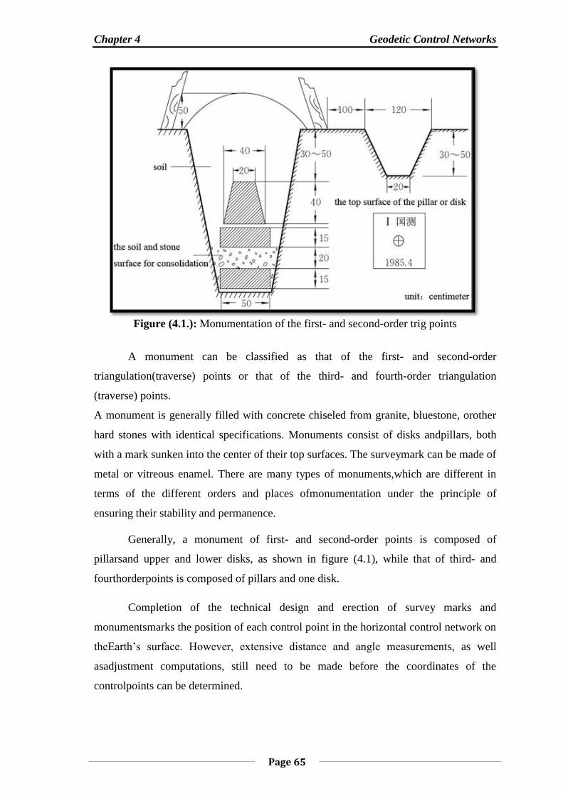
Chapter 4 Geodetic Control Networks
Page 65
Figure (4.1.): Monumentation of the first- and second-order trig points
A monument can be classified as that of the first- and second-order
triangulation(traverse) points or that of the third- and fourth-order triangulation
(traverse) points.
A monument is generally filled with concrete chiseled from granite, bluestone, orother
hard stones with identical specifications. Monuments consist of disks andpillars, both
with a mark sunken into the center of their top surfaces. The surveymark can be made of
metal or vitreous enamel. There are many types of monuments,which are different in
terms of the different orders and places ofmonumentation under the principle of
ensuring their stability and permanence.
Generally, a monument of first- and second-order points is composed of
pillarsand upper and lower disks, as shown in figure (4.1), while that of third- and
fourthorderpoints is composed of pillars and one disk.
Completion of the technical design and erection of survey marks and
monumentsmarks the position of each control point in the horizontal control network on
theEarth‟s surface. However, extensive distance and angle measurements, as well
asadjustment computations, still need to be made before the coordinates of the
controlpoints can be determined.

Chapter 4 Geodetic Control Networks
Page 66
4.4 The Egyptian Geodetic Control Network
The Egyptian Geodetic Control Network Between 1853 and 1859 a survey of
Egypt was made but did not depend on a triangulation scheme [Shaker, 1982]. Later,
many attempts were made for constructing a geodetic triangulation, but they were not of
higher order. In 1907 it became possible to begin a new work for establishing a geodetic
triangulation frame for Egypt, which is considered to be the first national network to be
established in Africa (Moritz, 1981). From the cost point of view, it was decided to
carry out the network along the Nile Valley only (Shaker, 1982). The main reason to
carry it out was to fix, with a great possible accuracy, fundamental control-stations to be
a base for the cadastral survey and national mapping of the country. Egyptian network
was extended to Sudan and other African Nations. The first order geodetic horizontal
control network of Egypt contains two main networks, Network (1) and Network (2),
(Cole, 1944). Figure (1.1) shows the first order triangulation networks.
4.4.1 Network (1)
It started in the year 1907 and was finished in 1945. It consists of ten sections
contain 195 stations and the general form as (T) shape, with initial point on the
Mokattem hills to the east of Cairo, figure (1.1). The nearly horizontal part from (T)
shape contains five sections covering the north area from Al-arish in the East to Al-
salom in the West and passing through Cairo region. The nearly vertical part from (T)
shape contains the other five sections covering the cultivated area of the Nile valley
from Cairo to Adindan near Sudanese borders. Each section starts from a base line and
ends at another base line. Station Z5 (Adindan) in the south is the origin of the Sudanese
geodetic network.
4.4.2 Network (2)
In 1952, the Egyptian Survey Authority (ESA) set out a plan for observing the
second geodetic Network (2) to cover South Sinai, the area of the Red sea, and to cover
also part of the Western Desert, in order to cultivate and inhabit these areas
(Elhussainy, 1982). Network (2) was constructed and observed from 1955 and finished
in 1968. This network consists of 207 stations forming three basic blocks which are
divided into 13 sections. The two Networks were linked by 19 common stations in
different regions, figures (1.1).

Chapter 4 Geodetic Control Networks
Page 67
4.4.3 Description of Treating Network 1 and Network 2
The geodetic observations of Network 1 and Network 2 were taken while the
geoid in Egypt was unknown. So the gravimetric reductions to the collected
observations were neglected. The gravimetric reductions are needed to relate the
observations to the ellipsoidal (geodetic) gravity field which the observations will be
computed in. The Network 1 is adjusted section by section, not as one block, so the
errors in the network are not homogeneously distributed. The coordinates of Network 2
stations are just computed from the collected observations without gravimetric
reductions and without any kind of adjustment. Therefore it is expected that Network 1
has some distortions and inconsistency. It is expected also that Network 2 has more
distortions and inconsistency.
4.5 . GPS Control Network
GPS can be used like any other surveying tool; it can accomplish certain goals if
we are conscious of its strengths and limitations. When surveying with GPS, we do not
need to have inter-visibility between the stations to measure a baseline. The only
constraint to receive the signals is having a clear view of the sky.
4.5.1 Principles for Establishment of GPS Control Networks
Establishment Based on Hierarchical Orders
Setting GPS network into different orders is conductive to stage-wise
establishmentaccording to the immediate needs and long-term development of survey
areas.Moreover, this principle enables the network structure to combine the long
andshort sides. Compared to the Short-Side GPS Control Network, the
networkestablished in such a way can reduce the accumulation of errors at its edge
andallows data processing and results checking of GPS networks to be carried outeasily
in a piecemeal fashion.
For instance, we can first use GPS to establish a nationwide high-
precisionbackbone control network with low density (A- and B-order networks or
firstandsecond-order networks) and then further densify the network using GPS

Chapter 4 Geodetic Control Networks
Page 68
orconventional methods based on the survey areas needed. In further densification,with
the help of GPS technology it is unnecessary to establish an overall geodeticnetwork in
advance. Instead, one can establish and use the network at any timeaccording to the
accuracy required by users. We can obtain directly the knownpoints from hundreds of
kilometers away by GPS measurement, which not onlysaves a lot of manpower and
material resources but also fulfills the practical needs.
Density
Different task requirements and service targets have different requirements
forestablishing the GPS network. For example, the national super-network (AA-order)
datum points are mainly used to provide national datums for orbit determination,precise
ephemeris calculations, and large-scale ground deformation monitoring,with an average
distance of hundreds of kilometers. The network required by ageneral engineering
survey with an average side length of several kilometers oreven shorter (within
hundreds of meters) should cater for the needs of mappingdensification and engineering
survey. Taking the above factors into account, a rulefor the distance between two
adjacent points in GPS networks is made dependent onvarious needs: the average
distance between adjacent points in GPS at all ordersshould meet the requirements of
the data in table (4.1); the shortest distance betweenadjacent points can be 1/3 to 1/2 of
the average distance while the longest is 2–3times. Under special circumstances,
depending on the network‟s task and target, thedistance between some points can
require specific rules for the distribution of GPSstations.
Accuracy
In the design of GPS networks, the order and accuracy standard should be
designedbased on the size of survey areas and the use of the networks. The accuracy
standardof general GPS measurement is commonly expressed by the mean square error
ofthe distance between adjacent points in the networks as follows:
Where: σ is the mean square error of distance (mm), a is the constant error
(mm), b isthe coefficient of the ratio error, and d is the distance between adjacent points

Chapter 4 Geodetic Control Networks
Page 69
(km).The national “GPS survey specifications” classify GPS measurement into
sixorders, namely AA, A, B, C, D, E (as shown in table 4.1). The Table lists
thedistances between points and their accuracy indicators in GPS networks of
differentorders (SBSM , 2009).
4.5.2 Technical Design of GPS Control Networks
Design of GPS Control Network Datum
The design of the GPS control network datum is fundamental to the
implementationof GPS measurement. It aims to find the best possible solution in terms
of accuracy, reliability, and economic efficiency of the network. With GPS
measurement we canobtain the GPS baseline vector between surface points, which
belongs to the three- dimensional coordinate system of WGS84 or ITRF. Practical
engineering applicationsrequire national coordinate systems like Beijing Coordinate
System 1954, Xi‟an Coordinate System 1980, China Geodetic Coordinate System 2000,
oranother independent local coordinate system. Therefore, in the technical design,the
coordinate system and the initial data of the GPS network have to be specified,which
means making clear the datum adopted by the GPS network.
The GPS network datum consists of position datum, azimuth datum, and
scaledatum. Position datum is usually determined by the coordinates of known
initialpoints. Azimuth datum can be determined by the value of the known
startingazimuth or the azimuth of the GPS baseline vector. Scale datum can be
determinedby the side of the electromagnetic wave distance measurement on the
Earth‟ssurface, by the distance between two initial points, or by the distance of the
GPSbaseline vectors. So, the design of the GPS network datum is essentially the issue
ofdetermining the position datum of the network.
Point Selection
Since GPS observation stations do not require intervisibility with each other,
theselection of points is much simpler than for conventional measurements. The
choiceof GPS points has a significant influence on the smooth operation of GPS
observationsand the acquisition of reliable results. As a result, we should collect and
fullyunderstand the geographical conditions of the survey areas and the distribution

Chapter 4 Geodetic Control Networks
Page 70
andmaintenance of existing control points based on the purpose of measurement andthe
requirements of coverage, accuracy, and density of the survey areas so as toproperly
choose the positions of the GPS points. The following principles should befollowed in
the selection of GPS point positions:
1. It should be convenient to install antennae and GPS receivers around the point.
The point should be located where the view is not obstructed and the elevation
angle of the surrounding obstacles is less than 15o.
2. The point should be far away from high-power radio emission sources and high
voltage wires to avoid interference from magnetic fields close to the signal.
3. In order to weaken multipath effects, there should be no objects that strongly
reflect or absorb electromagnetic waves around the point.
4. To improve operational efficiency, the point should be located where
transportation is convenient.
Table (4.1.): Accuracy and density of GPS control networks
5. Points should be selected taking into account the convenience of using other
measurement techniques for connection and extension.
6. The point should be located in solid soil or, better, an outcrop of rock in order to
be better preserved.
7. The integrity and stability of the survey mark should be checked before using
old points.
Additionally, other conditions such as the nearby communication facilities
andpower supplies should also be considered for the connections between points andthe
electricity for equipment.
4.6 Marking the Position of the GPS Control Point
For long-term preservation, the GPS control point should usually be located on
thesurvey mark (monument) with an identifier in the center to mark the point precisely.

Chapter 4 Geodetic Control Networks
Page 71
Both the survey mark and the identifier should be stable and firm. The mark can besunk
into the ground or built into an observation stake or a stake with forcedcentering
devices.
4.6.1 Monument for GPS Control Point
A large stone engraved with Circle and Dot, will be embedded in the ground firmly.
It will act as a lower mark. A cement concrete pillar of dimension 1m×1m×1.2m will be
constructed in such a manner that it is 0.7m below the ground level and 0.5m above
ground. A „Survey Reference Mark‟ made of Gun Metal/brass as shown in the figure
(4.2) will be embedded at the centre of pillar, flushed with the top surface of the pillar,
see figure (4.2)
Figure (4.2): Design of a good GPS network observation scheme

Chapter 4 Geodetic Control Networks
Page 72
4.6.2 Measurement Operations of GPS Control Networks
GPS measurement includes field observations and indoor data processing work.
The former consists of installation of antennae, observation operations, and recording of
field observation results whereas the latter consists of data extraction from instruments,
baseline solution, and adjustment calculations of three-dimensional GPS control
networks, etc. Below is an overview of field observations. For the extraction of
observation data and the indoor work of data processing, please refer to annexed
instructions and other relevant data (S.I.H.T, 2009).
Installation of Antennae
The precise installation of antennae is one of the prerequisites for precise
positioning and should satisfy the following conditions:
1. Normally, the antenna should be installed in the vertical direction of the mark
center on a tripod, directly centered. Only in exceptional cases can eccentric
observations be allowed, where the centering elements should be precisely
determined by analytical methods.
2. When installing an antenna on the platform of the tower, in order to avoid
interference to signals, the top of the tower should be removed and the mark
center be projected onto the platform. Then the antenna can be placed according
to the projection point.
3. When there is an ordinary tower at the point and the distance between
observation stations is less than 10 km, an antenna is allowed to be installed
upon the tower, but the time of observation should be extended.
4. The pointer of the antenna should be directed to the true north. The effect of
local magnetic declination should be considered and the orientation error should
be no more than ±5o.
5. The level bubble at the bottom of the antenna must be centered.
6. While installing an antenna in thunderstorm weather, the bottom of the antenna
must be grounded to avoid lightning strikes. In a thunderstorm, observation
operations should be stopped and the antenna removed.
After installation of the antenna, its height should be measured both before and
after each time interval of observation. The difference between the results of thetwo

Chapter 4 Geodetic Control Networks
Page 73
measurements should be less than 3 mm. The average can be determined as thefinal
height of the antenna. If the difference is larger than the tolerance, we should identify
the causes, put forward suggestions, and note down the observation records.
The antenna height refers to the height from the average antenna phase center to
the surface of the central mark of the observation station, which can be divided into two
parts. One part covers the height from the phase center to the bottom of the antenna (i.e.,
the antenna reference point, ARP), which is a constant provided by manufacturers; the
other part covers the height from the ARP to the surface of the central mark of the
observation station, which should be measured by users on thespot. The specific
measurement methods can be categorized into direct measurement and slant range
measurement, according to the methods and types of antenna installation. Please refer to
the receiver user manual for details. The final value ofthe antenna height is the sum of
the heights of the parts.
Observational Operations
Observational operations are mainly aimed at capturing, tracking, receiving,
andprocessing GPS satellite signals to obtain the required data on positioning
andobservations.The operation of GPS receivers is highly automated. Its specific
methods andprocedures of operation vary with the types and operating modes of
receivers.
Detailed information is included in the attached operation manuals. During
operation, observers only need to follow the instructions in the operation
manual.Generally, the following aspects should be noted:
1. Observers at each receiver should work within the regulated observation time to
ensure the realization of simultaneous observation of the same group of
satellites.
2. After correct connection of the external power supply, the cable and antenna are
confirmed, and the power can be switched on; when the receiver is in the right
preset state it can be started.
3. When the data on the receiver‟s panel display is normal, observers can begin the
self-test and input control information for observation stations and intervals of
observation time.

Chapter 4 Geodetic Control Networks
Page 74
4. When the receiver begins to record data, the observer should use function keys
and selection menus to check information on observation stations, number of
received satellites, satellite catalog number, channel SNR (signal-to-noise ratio),
phase measurement residuals, results and changes in real-time positioning,
records of storage media, etc.
5. During the period of observation, the receiver should not be turned off and
restarted. The antenna height and limits of the elevation angle of satellites
should not be changed. Observers are supposed to prevent vibration and
especially displacement of the receiving devices. The antenna or signals should
not be touched or obstructed.
6. When all the operation projects are confirmed to have been completed as
required, the station can be moved.
7. In long-distance GPS measurements at higher levels, meteorological elements
should be measured as required.
Observational Records
Observational records are automatically formed by GPS receivers onto
storagemedia, which include carrier phase observations, pseudo-range observations,
corresponding GPS time, parameters of GPS satellite ephemeris, clock
offsetparameters, and initial information of observation stations such as name,
cataloguenumber, time intervals, approximate coordinates, antenna height, and so on.
Theinformation on observation stations is generally first input by observers into
thereceivers or recorded manually in measurement handbooks (S.I.H.T, 2009).
Some GPS Networks in Egypt
GPS surveys for producing geodetic control points have been performed within
the Egyptian Survey Authority (ESA) through the Finnish Project in the Eastern Desert
(Finmap), the American Project in the Delta and along the River Nile with some
extensions in the Eastern Desert. In addition, the Survey Research Institute (SRI)
established some GPS points. Some other GPS control points were available from the
German Project in Aswan area. A High Accurate Reference Network (HARN) is
observed in 1995 and a new Egyptian Datum is based on it. GPS observations were
taken at triangulation stations in a project belong to the Aviation Authority. The
National Research Institute for Astronomy and Geophysics (NRIAG) established two

Chapter 4 Geodetic Control Networks
Page 75
GPS networks to follow the crustal movements in Sinai and Greater Cairo area in the
years 1994 and 1995 respectively.
4.7 Introduction to Network Adjustment
When performing network adjustments of GPS baselines, a least squares
adjustment of thegenerated baselines is often performed once processing is complete
and should follow themanufacturer‟s recommended procedures. These networks may
comprise static andkinematic baselines. The network adjustment procedure has several
functions in the GPSsurveying process. The adjustment provides a single set of
coordinates based on all themeasurements acquired, as well as providing a mechanism
by which baselines that have notbeen resolved to sufficient accuracy can be detected. A
series of loop closures should beperformed before the network adjustment procedure to
eliminate erroneous baselinesentering the adjustment process. A further feature of the
network adjustment stage is thattransformation parameters relating the GPS vectors to a
local coordinate system can beestimated as part of the adjustment. The adjustment
process can be done in several ways.The following sections highlight the major
elements of the adjustment process.
4.7.1 Minimally Constrained Adjustment
Once the processed Cartesian vectors have been loaded into the adjustment
module, anadjustment should be performed where one or no coordinates are
constrained. Theadjustment should be performed using the WGS84 datum and
appropriate estimates ofstation centering error. This solution provides a mechanism by
which GPS baselines, whichare not sufficiently accurate, can be detected. Once the
minimally constrained adjustmenthas been performed, the surveyor should analyze the
baseline residuals and statisticaloutputs (which will differ between adjustment
programs) and ascertain whether anybaselines should be removed from subsequent
adjustments. This process relies on thebaseline network being observed in such a
manner to ensure that redundant baselines exist.Redundant baselines enable erroneous
baselines.
4.7.2 Fully Constrained Adjustment

Chapter 4 Geodetic Control Networks
Page 76
Once the minimally constrained adjustment has been performed and all
unsatisfactorybaseline solutions removed, a fully constrained adjustmentcan be
performed. The constrained adjustment is performed to compute transformation
parameters, if required, and yield coordinates of all unknown points in the desired
coordinate system. The surveyor must ensure that sufficient points with known
coordinates are occupied as part of the survey. The user should analyze the statistical
output of the processor to ascertain the quality of the adjustment. Large residuals at this
stage, after the minimally constrained adjustment has been performed, will indicate that
the control points are non-homogeneous. It is, therefore, important that additional
control points are occupied to ensure that such errors can be detected.
4.7.3 Error Ellipses
The standard deviation of the estimated coordinates is derived from the inverse
of thenormal matrix generated during formulation of the least squares process. Error
ellipses foreach point can be computed from the elements of this matrix. The ellipse
presents a twostandard deviation confidence region (95% certainty) in which the most
probable solutionbased on the measurements will fall. Surveyors should base the quality
of the adjustmentprocess on the magnitude of these ellipses. Many contracts will specify
the magnitude oferror ellipses for both the minimally constrained and fully constrained
adjustments as amethod of prescribing required accuracy levels. The product
documentation for theadjustment program will further indicate the manner in which the
ellipse values aregenerated.
4.7.4 Independent Baselines (Non-Trivial Baselines)
For the least squares adjustment process to be successful, the surveyor must
ensure thatindependent baselines have been observed. If more than one session is used
to build thebaseline network, then independent baselines will exist. In instances where
one session isobserved and all baselines adjusted, the measurement residuals will all be
extremely small.
This is due to the correlation that exists between the baseline solutions as they
are derivedfrom common data sets. This is not a problem as long as the surveyor is
aware of theoccurrence and does not assume that the baselines are of as high accuracy
as implied fromthe network adjustment results. For each observing session, there are n-

Chapter 4 Geodetic Control Networks
Page 77
1 independentbaselines where n is the number of receivers collecting data
simultaneously, withmeasurements inter-connecting all receivers during a session. If the
mathematicalcorrelation between two or more simultaneously observed vectors in a
session is not carriedin the variance-covariance matrix, the trivial baselines take on a
bracing functionsimulating the effect of the proper correlation statistics, but at the same
time introducing afalse redundancy in the count of the degrees of freedom.
4.7.5 Error Analysis
The local accuracies of property corners are based upon the results of a least
squaresadjustment of the survey observations used to establish their positions. They can
becomputed from elements of a covariance matrix of the adjusted parameters, where the
known NSRS control coordinate values have been weighted using their one-sigma
networkaccuracies.
The 95% confidence circle representing a local accuracy can be derived from the
major andminor semi-axis of the standard relative ellipse between two selected points. It
is closelyapproximated from the major (a) and minor (b) semi-axis parameters of the
standard ellipseand a set of coefficients. For circular error ellipses, the circle coincides
with the ellipse. Forelongated error ellipses, the radius of the circle will be slightly
shorter than the majorsemi-axis of the ellipse. The radius of an error circle is equal tothe
major semi-axis of an associated error ellipse. The value of the largest error circle
radiusin the project should be adopted for reporting local project accuracy (Lee et al.,
1987; Paul and Charles, 1997 ; Rizos, 1996).
4.8 GPS Network Adjustments Procedures
4.8.1 Acquisition and check of GPS observation data
GPS observation data necessary for baseline processing and precise ephemeris of
GPS satellite necessary for baseline processing of long baseline should preferentially be
secured for GPS network adjustment. Besides, for accurate estimation of unknown point
coordinate with GPS network adjustment, the process of checking the quality of
observation data such asobserved antenna height, observed station name, receipt interval
of data & receipt time,receipt state of data is indispensable. Especially, in antenna
height case, checkup of thelocation that measured APC(Antenna Phase Center),

Chapter 4 Geodetic Control Networks
Page 78
ARP(Antenna Reference Point), and ofoffset of antenna receiver by manufacturer is
necessary. And a checkup of receiving time andstate needs to be done by all means for
the minute application of mathematical difference indifference to the observed value of
carrier value obtained from the two points while baselineprocessing. A checkup of
receipt time & receipt state is required for the minute application ofmathematical double
difference to the carrier wave observed value gotten from the two pointswhile baseline
processing.
4.8.2 GPS baseline processing
GPS network is adjusted by using 3-dimensional baseline vector between two
pointsgenerated from observed GPS data processing and VCV matrix. Baseline vector
and VCVmatrix can be calculated through GPS processing, a mathematical method and
procedureestimating baseline vectors ΔX, ΔY, ΔZ between two points by least square
method passingthrough the determination of integer ambiguity process after the
application of mathematicaldouble difference to the carrier wave observed value
obtained from the two points at the sametime effect of ionospheric and tropospheric,
error of satellite track need to be fully checkedup to raise the accuracy of baseline
processing, and baseline processing S/W should beselected suitable for the purpose for
use. Besides, after GPS processing, misclosure of baselinevector needs to be examined
if there exists outlier in baseline vector or not.
4.8.3 Minimally constrained adjustment
Minimally constrained adjustment is conducted to cover the following:
To detect outlier in GPS network that hasn't been detected in the miscloser
checkup that carried out after baseline processing,
to calculate approximate accuracy of GPS network, and
to determine the statistical model of GPS network that will be used in the
final adjustment.
One point fixed adjustment and free adjustment are mainly used for minimally
constrained adjustment, approximate accuracy of GPS network is assessed through
RMSE or arithmetic mean through calculation of the size of relative error ellipse
between points obtained after minimally constrained adjustment for certain
probability(generally 95%).

Chapter 4 Geodetic Control Networks
Page 79
4.8.4 Outlier detection (tau-test)
In order to checkup outlier within GPS network, standardized residual should be
calculatedunder the assumption that VCV matrix of measured value is unknown and
then compare themwith critical value determined by confidence interval and degree of
freedom supposing theyconform to students‟ distribution and then tau test was used for
outlier detection. Taudistribution is used to estimate the confidence interval of the
average of comparatively smallmother group, and mainly used to check up the propriety
of the average for certain part aftercomparison with the mother group average (Lee et
al., 1987; Paul and Charles, 1997).
4.8.5 Empirical stochastic modeling
Random error components could be included in the corrected VCV matrix, but
the errorsincluded in the estimation of effect of atmosphere and antenna height
estimation that haven'tbeen fully modeled in baseline processing S/W couldn't be
included in stochastic model, andso stochastic model is determined through Empirical
stochastic modeling which corrects thevariance, the diagonal element of VCV matrix by
recalculating it for reflection of actualaccuracy of GPS network. Empirical stochastic
modeling was done in the way of changing aand b in (4.1) by dividing it into
horizontal(N, E) and vertical(H) until it passed χ2 test, a fidelitytest for model. S is
standard deviation of baseline vector, a is absolute error different to thepoints observed,
b is relative error of ppm unit in proportion to baseline length, L is baselinelength
(Rizos, 1996).
(4-1)
4.8.6 Propriety test for stochastic model (χ2 test)
Stochastic test for variance factor is necessary for the propriety of mathematical
model andstochastic model that used for estimation or detection of outlier, and for this
test, attest forcertain confidence needs to be carried out. The result can‟t pass the χ2 test
if inappropriatemathematical model or stochastic model was used or the measured value
contains outlier.χ2 test is the density function for the distribution of variance estimated
from the degree offreedom selected by mother group, a critical value of distribution

Chapter 4 Geodetic Control Networks
Page 80
should be arranged into stochastic table for distribution use and stochastic test to
determine confidence interval for thevariance of mother group(Paul and Charles
,1997).
4.8.7 Over constrained adjustment
Over constrained adjustment is a way of determining the coordinate of unknown
point andfinal adjustment results by using the coordinate of unknown point and the size
of baselinevector between points & variation of VCV matrix. Function model,
determined by relationalexpression of coordinate difference for each baseline made up
of baseline vector is used forthe determined coordinate of unknown point by over
constrained adjustment. Function modelcould be formulated as observed equation and
in case, the number of observed equationexceeds that of unknown quantity, solution
could be obtained by least square methodprinciple(Lee et al., 1987; Leick, 2004;
Rizos, 1996).
4.8.8 Checkup of adjusted result and assessment of accuracy
The comparison of check result with reliable accuracy and coordinate difference
needs to beconducted along with comparison with individual applied point, and
stochastic calculationsuch as RMSE, standard deviation, mean for the coordinate
difference needs to be carried outfor the checkup of adjusted results. Besides, the
assessment of adjusted results accuracy isavailable through estimation of absolute error
ellipsoid generated from GPS networkadjustment. The accuracy of horizontal location
of absolute error ellipsoid could be seenconsidering the correlation of east and west (E)
and south and north (N), and the size andshape of error ellipsoid varies to the size of
standard deviation of measured value andcovariance between components.
Checkup and Analyze Loop Misclosure
Loop misclosure can be used to detect "bad" observations. (A bad observation
can includea misread antenna height, not being plumb over a point or observing the
wrong point). Iftwo loops with a common base line have large misclosure, this may be
an indication that thecommon base line is an outlier. Since users must repeat base lines
on different days and atdifferent times of the day, there are several different loops that
can be generated from theindividual base lines. If a repeat base line difference is greater

Chapter 4 Geodetic Control Networks
Page 81
than 2 cm then comparing theloop misclosure involved with the base line may help
determine which base line is theoutlier. According to NGS guidelines, if a repeat base
line difference exceeds 2 cm then oneof the base lines must be observed again, and base
lines must be observed at least twice ontwo different days and at two different times of
the day.
4.9 Adjustment of GPS Network Models
For the past five decades, NASA and the US military participated in space
research program a precise GPS navigation. System used six satellites of the first
generation, called transit countries, and is based on the Doppler principle. Transit is
available for commercial use in 1967, and shortly thereafter began to be used in the
survey. The creation of a global network of control centers between applications at the
earliest and the most valuable. GPS using transit required very long sessions control
point, and accuracy to level 1-m. Thus, in the survey it was only suitable for business
control over networks that consist of spaced points on a large scale. It was not
satisfactory to clear applications such as engineering or planning transit every day.
Encouraged by the success of transit, a new research program developed which
ultimately led to the creation of GPS in the NAVSTAR system (GPS). This system uses
GPS and navigation of the second-generation constellation of 24 satellites orbits.
Positioning accuracy have improved considerably compared to the transit system,
depriving the long monitoring sessions, also canceled. Although the developed
countries for military applications, and civilians, including surveyors, also found uses
the global positioning system.
Since its introduction, it used widely GPS. They are reliable and efficient and
able to generate a very high accuracy. Notes can be taken to determine the sites day or
night and in any weather. A great feature for GPS it is not necessary to see the dots
surveyed. Thus is avoided process takes a long time to scan the horizon lines. Al-
though most of the first applications of GPS in the work of monitoring, system
improvements now comfortable and practical for use in almost every type of study,
including surveys of ownership and topographic mapping, and staking of the building.
In practice, when surveys are done by observing carrier phases, four ormore satellites
are observed simultaneously using two or more receivers locatedon ground stations.
Also, the observations are repeated many times.

Chapter 4 Geodetic Control Networks
Page 82
This produces a very large number of redundant observations, from whichmany
difference combinations can be computed.Of the two GPS observing procedures,
pseudo ranging yields a somewhat lower order of accuracy, but it is preferred for
navigation use because it givesinstantaneous point positions of satisfactory accuracy.
The carrier-phase techniqueproduces a higher order of accuracy and is therefore the
choice forhigh-precision surveying applications. The differencing techniques used in
carrier-phase observations, describedbriefly above, do not yield positions directly for
the points occupied by receivers.Rather, baselines (vector distances between stations)
are determined.These baselines are actually computed in terms of their coordinate
differencecomponents ΔX, ΔY, and ΔZ. To use the GPS carrier-phase procedure in
surveying, at least two receiverslocated on separate stations must be operated
simultaneously. For example,assume that two stations A and B were occupied for an
observing session,that station A is a control point, and that station B is a point of
unknownposition. The session would yield coordinate differences ΔXAB, ΔYAB, and
ΔZABbetween stations A and B. The X,Y,Z coordinates of station B can then
beobtained by adding the baseline components to the coordinates of A as
XB=XA+ΔXAB
YB= YA+ ΔYAB (4.2)
ZB= ZA+ ΔZAB
Because carrier-phase observations do not yield point positions directly,but
rather, give baseline components, this method of GPS surveying is referredto as relative
positioning. In practice, often more than two receivers are usedsimultaneously in
relative positioning, which enables more than one baselineto be determined during each
observing session. Also, after the first observingsession, additional points are
interconnected in the survey by moving thereceivers to nearby stations. In this
procedure, at least one receiver is left onone of the previously occupied stations. By
employing this technique, a networkof interconnected points can be created. Figure
(4.3) illustrates an example of a GPS network. In this figure, stations A and B are
control stations,and stations C, D, E, and F: are points of unknown position. Creation
of suchnetworks is a common procedure employed in GPS relative positioning work.

Chapter 4 Geodetic Control Networks
Page 83
Figure (4.3): GPS survey network.
4.10 Continuously Operating Reference System
The Continuously Operating Reference System (CORS) is a major technique
forestablishing regional three-dimensional geodetic datums. Thanks to the rapid
development of satellite positioning technology, information technology, and
networktechnology, CORS networks have appeared all over the world, includingglobal
large-scale networks and regional small-scale networks. The classical horizontaldatum
is defined and extended by the geodetic origin and horizontal controlnetwork. Similarly,
the three-dimensional coordinate datum is defined andextended by CORS and GPS
networks (Hoffman-Wellenhof, 2001; Leick, 2004).
4.10.1 Basic Components of CORS
As the datum of the three-dimensional control network, CORS is the product
ofsophisticated new technologies, such as satellite positioning technology,
computernetwork technology, digital communication technology, and so on. It is
composedof a datum station network, see figure (4.4), data processing center, data
transmission system,positioning and navigation data broadcast system, and user
application system, see figure (4.5).

Chapter 4 Geodetic Control Networks
Page 84
Figure (4.4): The Monumentation of one Core Station

Chapter 4 Geodetic Control Networks
Page 85
Figure (4.5): The configuration of CORE networks
Every datum station is connected to the monitoring and analysis center through
thedata transmission system, constituting a special purpose network.
The datum station network, made up of datum stations distributed evenly
withina certain scope, is used to collect observational data from GPS satellites,
transmitthem to the data processing center, and provide services for monitoring the
systemintegrity.
The data processing center, as the control center of the system, is used to
receivedata from every datum station and form multiple datum stations‟ differential
positioning data for users through data processing. Then, the data files formed with a
certain format are distributed to users. The data processing center is the essential part of
CORS as well as the key to realizing high-precision real-time dynamic positioning.
After a continuous around-the-clock solution of the whole modeling within an
area based on real-time observational data collected by every datum station, the center
automatically generates a virtual reference station (including the coordinates of datum
stations and GPS observations) corresponding to the mobile station and provides
various users who are in need of measurement and navigation with code phase/carrier

Chapter 4 Geodetic Control Networks
Page 86
phase differential correction information in a universal common format via the existing
data communication networks and wireless data broadcast systems so as to calculate the
exact real-time position of mobile stations.
The data transmission system, where data from every datum station are
transmitted to the monitoring and analysis center through fiber lines. The system
comprises hardware devices for data transmission and software control module. The
data broadcast system broadcasts positioning and navigation data to users in the form of
mobile networks, UHF radio, Internet, etc.
The user application system consists of a user information receiving system,
anetwork-based RTK (real-time, kinematic) positioning system, a fast and
postprocessingprecision positioning system, an autonomous navigation system,
positioningmonitoring system, and so on. According to different application
accuracies,the user service subsystem ranges from millimeter-level, centimeter-
level,decimeter-level, to meter-level whereas, according to different user applications,
itcan be categorized into surveying and mapping and engineering users
(centimeteranddecimeter-level), vehicle navigation and positioning users (meter-level),
highprecisionusers (post-processing), and meteorology users.
CORS is not only a kinematic and continuous positioning reference frame
butalso an important technical means for rapid and high-precision acquisition of
spatialdata and geographic features. CORS is more often applied in small areas,
forinstance, a city, to provide three-dimensional datum. Within an area, it
provideshighly precise, reliable, and real-time positioning information to a large number
ofusers simultaneously and unifies the surveying and mapping data in the city.
Forexample, the application of CORS in cities will exert a profound and
lastinginfluence on the collection of modern urban geographic information and
theapplication system. Not only can it establish and maintain a reference frame ofthe
surveying and mapping in cities, it can also provide automatically all-weatherreal-time
spatial and temporal information of high-precision, serving as the basis ofregional
planning, management, and decision-making. It can also provide differentialpositioning
information and develop new applications of transportationnavigation; again it enables
high-precision, high-spatial-and-temporal-resolution,all-weather, near-real-time, and
continuous variable sequences in precipitable watervapor, which will gradually form a

Chapter 4 Geodetic Control Networks
Page 87
regional severe weather monitoring and forecastingsystem. CORS can also be used in
the high-precision time synchronizationin communication and power systems and will
provide the services of monitoringand predicting land subsidence, geological disasters,
and earthquakes and will studythe temporal and spatial evolution of natural disasters.
Currently, CORS systems have been established in many developed countries
worldwide, Egypt, KSA, UAE, Bahrain and Jordan(Zhiping Lu,& at el,2014).
4.10.2 CORS Network in Egypt
NRIAG CORE NETWORK
In 2006, NRIAG started the establishment of the Egyptian Permanent GPS
Network (EPGN). Basically, the site selection was aimed to cover geographically all the
Egyptian territory but also considering the tectonic setting of Egypt. As shown in
figure(4.6), three stations were located in the Eastern Desert at the Red Sea coast, two
stations in Sinai Peninsula, four stations in the Western Desert, three stations at the Nile
and six stations around Cairo and the Nile Delta.

Chapter 4 Geodetic Control Networks
Page 88
Figure (4.10.): Geographic distribution of the NRIAG CORE Network
The EPGN operation started by four stations in 2007 to 18 stations was
achievable at the end of 2014 (4 in 2007, 2 in 2008, 3 in 2010, and 6 stations in 2011,
three station in 2014). In addition to these 18stations, it was started 2015 to install
another four stations in south of Aswan two in Eastern side of Nasser Lake, and two in
the western side of the lake to continuous monitor of seismic activities around the High
Dam(A.F.R.E.F,2007).
ESA CORE NETWORK
Unfortunately, nothing was published about it. What is known that ESA started
installing it 2008 and consists of 40 CORE station covered the Nile Delta and Nile
Valley, most of it, installed on the branches of ESA in different Governorates with
Trimble NET R5 GNSS receivers.

Chapter 5 Experimental Results & Evaluation
Page 89
Chapter Five
Experimental Results & Evaluation
In space geodetic positioning, where the observation techniques provide absolute
positions with respect to a consistent terrestrial reference frame, the corresponding
precise definition and realization of terrestrial and inertial reference systems is of
fundamental importance. Thanks to significant improvements in receiver technology, to
extension and densification of the global tracking network along with more accurate
determination of positions and velocities of the tracking stations and to dramatically
improved satellite orbits, GPS is today approaching 0.1 ppm precision for longer
baselines and it can be considered to be the main global geodetic positioning system
providing nearly instantaneous three-dimensional position at the cm accuracy level. One
of the fundamental goals of geodesy is to precisely define positions of points on the
surface of the Earth, so it is necessary to establish a well-defined geodetic datum for
geodetic measurements and positioning computations. Recently, a set of the coordinates
established by using GPS and referred to an international terrestrial reference frame
could be used as a three-dimensional geocentric reference system for a country (Chang
and Tseng, 1998b).
In the classical sense, a geodetic datum is a reference surface, generally an
ellipsoid of revolution of adopted size and shape, with origin, orientation, and scale
defined by a geocentric terrestrial frame. Once an ellipsoid is selected, coordinates of a
point in space can be given in Cartesian or geodetic (curvilinear) coordinates (geodetic
longitude, latitude, and ellipsoid height).
Two types of geodetic datum can be defined namely a static and kinematic
geodetic datum. A static datum is thought of as a traditional geodetic datum where all
sites are assumed to have coordinates which are fixed or unchanging with time. This is
an incorrect assumption since the surface of the earth is constantly changing because of
tectonic motion. Static datum does not incorporate the effects of plate tectonics and
deformation events. Coordinates of static datum are fixed at a reference epoch and
slowly go out of the date, need to change periodically which is disruptive.
89

Chapter 5 Experimental Results & Evaluation
Page 90
Datum's can either become fully kinematic (dynamic), or semi-kinematic. A
deformation model can be adopted to enable ITRF positions to be transformed into a
static or semi-kinematic system at the moment of position acquisition so that users do
not see coordinate changes due to global plate motions. GNSS devices which use ITRF
or closely aligned systems position users in agreement with the underlying kinematic
frame, however, in practice there are a number of very significant drawbacks to a
kinematic datum. Surveys undertaken at different epochs cannot be combined or
integrated unless a deformation model is applied rigorously, or is embedded within the
data, and the data are correctly time-tagged. On the other hand, Semi–Kinematicdatum
incorporates a deformation model to manage changes (plate tectonics and deformation
events). Coordinates fixed at a reference epoch, so the change to coordinates is
minimized. Many countries and regions which straddle major plate boundaries have
adopted a semi-kinematic (or semi-dynamic) geodetic datum in order to prevent
degradation of the datum as a function of time due to ongoing crustal deformation that
is occurring within the country.
High precision GNSS positioning and navigation is very rapidly highlighting the
disparity between global kinematic reference frames such as ITRF and WGS84, and
traditional static geodetic datum. The disparity is brought about by the increasingly
widespread use of PPP and the sensitivity of these techniques to deformation of the
Earth due to plate tectonics. In order for precision GNSS techniques to continue to
deliver temporally stable coordinates within a localized reference frame.
5.1 Transformation Parameters Terrestrial Reference Systems “TRS”
Recall that Transformations from kinematic ITRF to a static datum are
conventionally done by either using the site velocity (measured directly or computed
from a plate motion model) to compute the displacement between the reference and
current epochs or by a conformal transformation augmented with time dependent
parameters to account for rigid plate motion. Rigid Plate movement is conventionally
defined by a rotation rate about an Euler Pole and , where , are the latitude and
longitude of the pole, and is the rate of rotation of the plate around the pole in degrees
per million years. Equivalent rotation rates about the Cartesian axes ( and ) can
be computed from the Euler pole definition using equations (5.1-5.3) ( , , and ) are
first converted from decimal degrees to radians):

Chapter 5 Experimental Results & Evaluation
Page 91
Ω (Φ) ( ) (5.1)
Ω (Φ) ( ) (5.2)
Ω (Φ) (5.3)
A site velocity in Cartesian format ( ) can be computed for any given
location (X, Y, Z in meters) on a rigid plate defined by (ΩX, ΩY, ΩZ in radians per
million years) using:
[
] [
Ω Ω Ω Ω Ω Ω
] 1E-6 (5.4)
By introducing a reference epoch and an epoch of measurement t (epochs in
decimal years), the ITRF coordinates of any point on a rigid plate at a reference epoch
( , , in meters) can be computed from the coordinates at epoch t ( , , in
meters) using:
[
] [[
] [
] ( ) ] (5.5)
For any location on a rigid plate, instantaneous ITRF coordinates can be transformed to
a fixed reference epoch using equation (5-18) (Stanaway and Roberts, 2009).
[
] [
] [[
] [
Ω Ω Ω Ω Ω Ω
] ( ) ] (5.6)
Where:
( ): are the ITRF Cartesian coordinates at the reference epoch
(in decimal years),
( ): are instantaneous ITRF Cartesian coordinates at epoch (epoch
in decimal years),

Chapter 5 Experimental Results & Evaluation
Page 92
( ): is the translation of the reference frame origin (from ITRF to
local system),
(Ω Ω Ω ): are the Cartesian rigid plate/block rotation parameters, is the
reference frame
: is scale factor (from ITRF to local).
As it is seen in figure (5.1), the African continent is broadly divided into two major
tectonic plates. Most of Africa, west of the East African Rift lies on the Nubian Plate.
The Somalian Plate lies east of the African Rift. A very small section of North Africa
along the Maghreb coast in Algeria and Morocco lies on the Eurasian Plate and the
Dankalia region of Eritrea lies on the Arabian Plate.
Figure (5.1.): The Africa tectonics sub-plates
Analysis of the ITRF2005 solution (Altamimi et al., 2007; IERS, 2010)
indicates that ITRF site velocities for any location within Africa are between 24 and 31
mm/yr due to rigid motion of the African plates over the underlying mantle. These site
velocities degrade the accuracy of absolute positions like PPP if the measurement epoch

Chapter 5 Experimental Results & Evaluation
Page 93
is misinterpreted as a reference epoch for the underlying datum realization in use at the
time Equations (5.1, 5.2 and 5.3) were used to compute (ΩX, ΩY, ΩZ) for the Nubian
Plate using the Euler parameters determined by ITRF2008 PMM “Plate Motion Model”
(Altamimi Z., et al. (2012) and Egypt‟s Deformation Model (Saleh,M. , Becker, M.,
2013), the results were depicted in table (5.1).
Table (5.1.): The Cartesian angular Velocity of Nubian Plate
Deformation
Model
Absolute Pole Cartesian angular Velocity for Nubian Plate
(Rad/Ma) (Rad/Ma) (Rad/Ma)
ITRF2008-PMM 0.000461 -0.00290 0.003506
5.2. PPP Solution
PPP has received increased attention in the past several years within the GPS
community due to its great operational flexibility and accuracy promise. The major
advantages of PPP lie in two aspects: system simplicity at the user‟s end and global
consistency in terms of positioning accuracy. PPP-based approach significantly reduces
the equipment and personnel costs, pre-planning, and logistics compared to
conventional GPS network-based approaches. Applying PPP, a single survey team can
establish a CORS network across a PPP has received increased attention in the past
several years within the GPS community due to its great operational flexibility and
accuracy promise (A. Elhattab, 2014).
The major advantages of PPP lie in two aspects: system simplicity at the user‟s
end and global consistency in terms of positioning accuracy. PPP-based approach
significantly reduces the equipment and personnel costs, pre-planning, and logistics
compared to conventional GPS network-based approaches. Applying PPP, a single
survey team can establish a control network across a large area, rather than the
complicated logistics and communications needed to organize multiple survey teams to
occupy stations simultaneously. It also reduces the needs to analyze the data using
scientific software packages, which are not generally too accessible to inexperienced
users.

Chapter 5 Experimental Results & Evaluation
Page 94
Measurements from the IGS global tracking network are processed by the IGS
Analysis Centers to provide the highest quality satellite orbit and clock parameters.
These parameters are freely available from the Internet and are the basis for PPP
development. These IGS products can be applied to significantly reduce the errors in
GPS satellite orbits and clocks, which are two of the most significant error sources in
GPS positioning. Combining precise satellite positions and clocks with a dual frequency
GPS receiver to remove the first order effect of the ionosphere, PPP is able to provide
position solutions at centimeter level. Coordinates estimated with PPP will be in the
same global reference frame as the satellite orbits. When using orbits from IGS,
estimated receiver coordinates are referred to the IGS realization of ITRF.
Last decades several PPP post-processing software have been developed based
on the above observation models. Also online web services from different organizations
such as the Precise Point Positioning Software Center (http://gge.
unb.ca/Resources/PPP/index.htm) which has been created under the auspices of the
Canadian Geomatics for Informed Decisions Network of Centers of Excellence
provides users easy access to online PPP services as CSRS-PPP
by Natural Resources Canada (NRCan),GPS Analysis and Positioning Software
(GAPS)by University of New Brunswick (UNB),Automatic Precise Positioning Service
(APPS)by Jet Propulsion Laboratory (JPL),and magic GNSS by GMV (privately owned
technological business group).
5.2.2 Evaluating the PPP Solution
The solution of CSRS-PPP SW is now used extensively to provide realizations
of ITRF globally with a precision of a few centimeters. Four groups of data from IGS
stations, namely MALI (Malindi, Kenya) on the Somalian plate, RABT (Moracco) on
the Nubian plate, RAMON (occupied Palestine) on the Arabian plate and NICO
(Nicosia, Cyprus) on the Eurasian plate, distributed over the different sub-plates of
Africa and their positioning was computed and published by the IGS data centers at
ITRF 2008 Epoch2005 and given in table (5.2). The data of the four groups of IGS
stations was downloaded from ftp://garner.ucsd.edu/pub/rinex/2015/100/ for Day 100,
2015 and processed using the Precise Point Positioning module of CSRS-PPP. To
transfer the IGS published coordinates from Epoch2005, as: = 2005, to the epoch of

Chapter 5 Experimental Results & Evaluation
Page 95
the PPP solutions, ITRF 2008 Epoch2015.274 as t, Epoch2015.274, the following
formula (Altamimi. Z, 2006), is used:
P ( t0 ) = P( t ) + P˙( t0- t) (5.7)
Where:
P(t0) = is the positioning at a reference epoch ITRF 2008 Epoch 2005
P(t) = is the positioning value at time t, defined by PPP at epoch 2015.274
P˙ = Velocity
Table (5.2.): ITRF2008 STATION POSITIONS AT EPOCH 2005.0 AND
VELOCITIES
DOMES
SITE
X/Vx Y/Vy Z/Vz Sigmas
--------------------/m/y-----------
35001M002 Rabat RABT 5255617.683 -631745.687 3546322.552 0.001 0.001 0.001
35001M002 -0.0088 0.0174 0.0142 0.0001 0.000 0.0001
33201M001 MALINDI MALI 4865366.354 4110737.599 -331121.569 0.001 0.001 0.001
33201M001 -0.0172 0.02 0.0167 0.0001 0.0001 0.0000
20703S001 Mitz
RAMON RAMO 4514721.855 3133507.841 3228024.716 0.001 0.001 0.001
20703S001 -0.0205 0.0141 0.0177 0.0001 0.0001 0.0001
14302M001 NICOSIA NICO 4359415.713 2874117.066 3650777.829 0.001 0.001 0.001
14302M001 -0.0179 0.0116 0.0126 0.0001 0.0001 0.0001
The transferred coordinates of the four IGS stations defined in ITRF2008 Epoch
2015.274 are tabulated in table (5.3).
Table (5.3.): IGS Data Set Expressed in ITRF2008 Frame Station Positions and
Velcocities at Epoch 2015/04/10
DOMES NB SITE
NAME ID
SOL
N X Y Z
SIGMA
x
SIGMA
y
SIG
MA z
35001M002 RABTRABT 1 5255617.683 -631745.687 3546322.552 0.001 0.001 0.001
33201M001 MALINDI MALI 1 4865366.177 4110737.805 -331121.398 0.001 0.001 0.001
14302M001
NICOSIA-
ATHALASS
A
NICO 1 4359415.525 2874117.189 3650777.949 0.001 0.001 0.001
20703S001 Mitzpe
Ramon
RAM
O 1 4514721.645 3133507.986 3228024.898 0.001 0.001 0.001

Chapter 5 Experimental Results & Evaluation
Page 96
To see how the PPP can be used in updating the ITRF of the IGS points, the
solution of PPP with the transferred published IGS ITRF2008 at Epoch 2015.274 are
given in table (5.4). The differences between two solutions are computed and outlined
in table (5.4). As it is shown in the table, the absolute value of the maximum differences
does not exceed 17mm for the Y component of Nico Station, while does not exceed few
mm for the other stations.
Table (5.4.): the updated positioning for four IGS stations defined in ITRF2008 epoch
2015.274 by IGS & PPP
Rabat
Sol. Type X Y Z
PPP- Solution 5255617.590 -631745.508 3546322.700
IGS-Solution 5255617.593 -631745.508 3546322.698
Differences -0.003 0.000 0.002
Mali
Sol. Type X Y Z
PPP- Solution 4865366.174 4110737.798 -331121.393
IGS-Solution 4865366.177 4110737.805 -331121.398
Differences -0.003 -0.007 0.005
Nico
Sol. Type X Y Z
PPP- Solution 4359415.522 2874117.172 3650777.950
IGS-Solution 4359415.525 2874117.189 3650777.949
Differences -0.003 -0.017 0.001
Ramo
Sol. Type X Y Z
PPP- Solution 4514721.636 3133507.978 3228024.886
IGS-Solution 4514721.641 3133507.982 3228024.891
Differences -0.005 -0.004 -0.005
By comparing the differences of the two solutions for the four IGS stations, one
can easily see that, how the PPP is precise in expressing the epochwise solution of the
ITRF frame.
Additionally to see for what extent PPP can be an alternative for the differential
techniques, seven test points were processed by Trimble Business Center “TBC”
Software, the product of Trimble, with considering the PPP solution of PHLW as a
reference station for the processing. The results of the processing were demonstrated in
table (5.5).

Chapter 5 Experimental Results & Evaluation
Page 97
As it is shown in table (5.5), one can easily see the quality of PPP solution
compared with the DGPS solution. In spite of the processed baselines are exceed
several tens of kilometers to 120 km, PPP shows good harmony with the DGPS in mm
level except the station 0Z20 which has differences of 2.3 to 3.2 cm that may be it has
the longest baseline as well as it gives the worst accuracy of PPP that is may be come
from the surrounding environments around the station.
Table (5.5.): The differences between DGPS & PPP solutions for the observed Stations
St.
DGPS Sol.
PPP Sol.
Differences bet
DGPS & PPP
X Y Z X Y Z dX dY dZ
PHL
W 4728141.180 2879662.608 3157147.159
4728141.180 2879662.608 3157147.159
0.000 0.000 0.000
0Z18 4657081.787 2807150.058 3322370.152 4657081.784 2807150.059 3322370.156 0.003 -0.001 -0.004
0Z20 4796793.729 2651830.764 3250924.993 4796793.697 2651830.738 3250924.970 0.032 0.026 0.023
0Z89 4745737.252 2795140.347 3205858.805 4745737.246 2795140.341 3205858.797 0.006 0.006 0.008
0Z94 4739314.560 2828743.551 3186027.207 4739314.553 2828743.544 3186027.199 0.007 0.007 0.008
Burg 4765954.276 2704546.183 3252949.202 4765954.269 2704546.174 3252949.193 0.007 0.009 0.009
O1 4728219.038 2879743.411 3156930.682 4728219.033 2879743.402 3156930.676 0.005 0.009 0.006
5.3. The Evaluation Study
In 1992, an ESA steering committee developed a plan for the creation of new
datum for Egypt, with the following approach (Scott, 1997):
First, observe approximately 30 stations at approximately 200 km interval,
covering all of Egypt, creating a High Accuracy Reference Network (HARN).
Both high absolute and relative accuracies are required for these stations.
Second, establishing the Notational Agricultural Cadastral Network (NACN)
relative to these 30 stations, covering the green area of Egypt (Nile Valley and
the Delta) at 30-40 km intervals. This station spacing was selected to allow for
further densification with single frequency receivers, see figure (1.2).
Third, densify this network at a station spacing of approximately 5 km for use as
cadastral control at the governorate level.
Finally, replace the existing Egyptian Mercator grid with a new modified UTM
coordinate system.

Chapter 5 Experimental Results & Evaluation
Page 98
The ITRF1994 was transferred to Egypt‟s HARN network by connecting it with
four IGS stations, namely MATE (Italy), KIT3 (Uzbekistan), HART (South Africa) and
MASP in (Canary Island), depicted in chapter one figure (1.3). Each HARN‟s station
was observed for six sessions, every session was 6 hours with 30 seconds epoch
interval. The observation time was planned to produce 1:10,000,000 (Order A) for
HARN and 1:1,000,000 (Order B) for NACN relative network accuracy standard
between stations. The results of analyzing both of them were defined in ITRF1994
epoch 1996.
To see for what extent can the PPP be an alternative for the differential
techniques and its impact in analyzing the geodetic applications that need an ultimate
accuracy like the National High Accuracy Reference Networks, a critical example is
given to demonstrate this study. The example is concerned with analyzing a part of
Egypt HARN and NACN (National Agriculture Cadastre) Networks that is located in
and around Nile Delta. The geometric location of this part is illustrated in figure (5.2)
and the position of the aforementioned points as given in HARN analysis report (Scott,
1997) is depicted in table (5.6). Additionally, this section deals with the computing
techniques that are used in transferring the terrestrial frame from epoch to epoch in to
different frames. Three days campaigns were conducted in June 2015 from 3 to 6, to
convert this part of HARN & NACN network in the most recent ITRF available frame
at the epoch of observation campaigns, namely ITRF 2008 epoch 2015.422. However,
we use the aforementioned approach, equation (5.7) in transferring the PPP solution of
the specified part of HARN to the ITRF 2000 epoch 2000, utilizing the three
parameters of Nubian plate as defined by ITRF2005-PMM (Altamimi et al. (2007).,
table (5.1). The results are given in table (5.7).
Table (5.6.): The coordinates of chosen points of the HARN and NACN Networks
ITRF 1994, epoch 1996 (Scott, 1997).
Station X Y Z
OZ94 4745737.755 2795140.173 3205858.575
OZ89 4739315.089 2828743.36 3186026.976
OZ18 4657082.606 2807149.887 3322369.803
OZ20 4796794.204 2651830.557 3250924.750

Chapter 5 Experimental Results & Evaluation
Page 99
Figure (5.2): The location of the used part of Egypt HARN & NACN
Table (5.7.): The Part of HARN & NACN network updated in ITRF2000
ST.
PPP Results Coordinate at Epoch 2015.422
Transformed PPP Coordinates at ITRF2008
Epoch 2005
X Y Z X Y Z
PHLW 2879662.632 2879662.632 3157147.186 2879662.851 2879662.483 3157147.019
0Z18 4657081.784 2807150.059 3322370.156 4657082.003 2807149.91 3322369.989
0Z20 4796793.697 2651830.738 3250924.970 4796793.916 2651830.589 3250924.803
0Z89 4745737.246 2795140.341 3205858.797 4745737.465 2795140.192 3205858.63
0Z94 4739314.553 2828743.544 3186027.199 4739314.772 2828743.395 3186027.032
Burg 4765954.269 2704546.174 3252949.193 4765954.488 2704546.025 3252949.026
O1 4728219.033 2879743.402 3156930.676 4728219.252 2879743.253 3156930.509
The evaluation strategy is based upon:
1. Evaluating the IGS stations that were used in transferring the ITRF to HARN,
by using their published ITRF2008 Epoch2015.422 coordinates values and the
related transformation parameter to ITRF1994 Epoch1996 and compares the
transferred values by the reported values of (Scott, 1997).
2. Transferring the values of HARN & NACN networks that were defined in
ITRF2008 epoch 2005 to the original ITRF frame of HARN, namely ITRF1994
epoch 1996 and compare the resulted values with the original coordinate‟s
values given by (Scott, 1997). The aforementioned transformation is performed

Chapter 5 Experimental Results & Evaluation
Page 100
by exploiting the published 14 transformation parameters between different
ITRF‟s Frames by IGS (John, D.and Jim S., 2004). However, the
transformation process from ITRF 2008 epoch 2015.422 to ITRF 1994 epoch
1996 will be performed in the following steps:
1. Transforming the PPP values of HARN & NACN networks that defined in
ITRF2008 epoch 2015.422 to ITRF2008 Epoch2005 using the published
Absolute Pole Cartesian angular Velocity for Nubian Plate, as outlined
before.
2. Transferring the ITRF2008 Epoch2005 to ITRF1994 Epoch 2000 using the
published parameters in table (5.8).
3. Updating the values specified in the table (5.8) to be in Epoch 1996 instead
of Epoch2000.
4. Compute the differences
Table (5.8.): Transformation parameters Between ITRF2008 Epoch 2005 to ITRF 1994
Epoch 2000
EPOCH R1
R1
R1
D
Ppb
T3
mm
T2
mm
T1
mm
SOLUTIO
N
UNITS…
…
/Y
/Y
/Y
Ppb/Y
mm/Y
mm/y
mm/y
RATES
UNITS…
…
2000 0.06
0.02
0.00
0.00
0.00
0.00
2.92
0.09
-33.2
-3.2
2.6
-0.05
4.8
0.1
ITRF94
rates
5.3.1 Evaluating the IGS Stations that was Used in Transferring the
ITRF to HARN
Before digging into applying the above procedures, a check for the published
transformation parameters are done. This step is so necessary to check the quality of the
published data by IGS as well as to see the size of errors embedded in the stations that
were used by (Scott, 1997) in transferring the ITRF1994 frame to Egypt‟s HARN,
namely MATE (Italy), KIT3 (Uzbekistan), HART (South Africa) and MASP in
(Canary Island), see figure (1.3). table (5.9) depicts the coordinates of the four IGS
stations defined in ITRF1994 Epoch 1996 as given by (Scott, 1997) and the published
by IGS in ITRF2008, Epoch2005.

Chapter 5 Experimental Results & Evaluation
Page 101
It was stated in http://itrf.ign.fr/rel_trs.php that the standard relation of
transformation between two reference systems is an Euclidian similarity of seven
parameters: three translation components, one scale factor, and three rotation angles,
designated respectively, T1, T2, T3, D, R1, R2, R3, and their first times derivations: 1,
2, 3, , 1, 2, 3. The transformation of coordinate vector X1, expressed in a reference
system (1), into a coordinate vector X2, expressed in a reference system (2), is given by
the following equation:
(5.8)
With: (
) and (
)
It is assumed that equation (5.7) is linear for sets of station coordinates provided
by space geodetic technique (origin difference is about a few hundred meters, and
differences in scale and orientation are of 10-5 level). Generally, X1, X2, T, D, R are
function of time. Differentiating equation (5.7) with respect to time gives:
(5.9)
D and R are of 10-5
level and is about 10 cm per year, the terms D 1 and
R 1 arenegligible which represent about 0.0 mm over 100 years. Therefore,
equation (5.9) could be written as:
+ (5.10)

Chapter 5 Experimental Results & Evaluation
Page 102
Table (5.9.): The coordinate values of the IGS four stations in ITRF1994, Epoch 1996
and the published coordinate values for the nominated IGS stations in ITRF2008
Epoch2005
Statio
n ITRF2008 Epoch2005
ITRF1994 Epoch 1996 (as given by
Scott, 1997)
MATE 4641949.557 1393045.422 4133287.465 4641949.737 1393045.262 4133287.317
KIT3 1944945.139 4556652.244 4004326.007 1944945.390 4556652.199 4004325.973
HART 5084625.288 2670366.383 -2768494.401 5084625.460 2670366.404 -2768494.470
MAS1 5439192.215 -1522055.484 2953454.847 5439192.277 -1522055.641 2953454.694
The four stations in table (5.7) were transferred from ITRF2008 Epoch2005 to
ITRF1994 Epoch2000 using the transformation parameters given in table (5.8) and
equation (5.8). The results were demonstrated in table (5.10). Also the velocities of the
specified IGS stations in ITRF1994 were also depicted in table (5.10).
Table (5.10.): The transferred coordinate values of the four stations to ITRF1994
Epoch2000
Station ITRF1994 Epoch2000 Velocity m/y
MATE 4641949.557 1393045.429 4133287.444 -0.0191 0.0202 0.0121
KIT3 1944945.149 4556652.26 4004325.985 -0.028 0.0163 0.0064
HART 5084625.308 2670366.394 -2768494.442 -0.0015 0.0164 0.018
MAS1 5439192.236 -1522055.486 2953454.822 0.0001 0.0154 0.0152
To transfer the computed IGS coordinates from Epoch2000, as: = 2000, to the
epoch of the HARN solutions, ITRF 1994 Epoch1996 as t, equation (5.7) was used. The
results of the transformation were given in table (5.11). To see the differences between
the original coordinate values of the used IGS four stations as given by Scott (1997),
defined in ITRF1994 Epoch1996, as outlined in table (5.7), the differences between the
two ITRFs were computed and recorded in table (5.11) and the differences in table
(5.12).
Table (5.11.): The values of the published coordinate values of the four IGS stations &
the reported values by (Scott, 1997) in ITRF1994 Epoch1996
St.
ITRF1994 Epoch1996 transferred from IGS
published values in ITRF2008 Epoch2005
ITRF1994 Epoch1996 as reported by Scott
(1997)
X Y Z X Y Z
MATE 4641949.633 1393045.348 4133287.396 4641949.737 1393045.262 4133287.317
KIT3 1944945.261 4556652.195 4004325.959 1944945.390 4556652.199 4004325.973
HART 5084625.314 2670366.328 -2768494.514 5084625.460 2670366.404 -2768494.470
MAS1 5439192.236 -1522055.548 2953454.761 5439192.277 -1522055.641 2953454.694

Chapter 5 Experimental Results & Evaluation
Page 103
Table (5.12.): The differences between the published coordinate values of the four IGS
stations & the reported values by (Scott, 1997) in ITRF1994 Epoch1996
St.
Differences
Bet. ITRF1994 Epoch1996 transferred from IGS published values in ITRF2008
Epoch2005&ITRF1994 Epoch1996 as reported by Scott (1997)
dX dY dZ
MATE 0.104 -0.086 -0.079
KIT3 0.129 0.004 0.014
HART 0.146 0.076 0.044
MAS1 0.041 -0.093 -0.067
As it is shown in table (5.12), in spite of we have already used only in the
previous processing the published values and models as specified by IGS, one can see a
tolerance ranged between -8.6 cm to 14.6 cm. The reasons behind these differences are
mostly returning to the limited number of stations, only 13 stations - see figure (5.4)-,
that were used in realizing the ITRF94 that leads to sub-optimal stations distribution and
small discontinuities between IGS realizations of ITRF, as clarified by (Ferland and
Kouba, 1996).
Figure (5.3): Station set (13) used for IGS Realization of ITRF 92-93-94

Chapter 5 Experimental Results & Evaluation
Page 104
5.3.2. Transferring the Solved PPP Part of HARN Network to the
ITRF 1994 Epoch 1996
Firstly, transfer the tested part of HARN and NACN from ITRF2008
epoch2005, specified in table (5.5), to HARN ITRF1994 epoch 2000, with the
aforementioned steps in sub-chapter 5.4 by using equation (5.8) and table (5.8).The
computation results are given in table (5.13).
Table (5.13.): The Results of Transformation the HARN to ITRF 1994 Epoch 1997
St. PPP at ITRF2008 Epoch 2005 PPP at ITRF1994Epoch 2000
X Y Z X Y Z
PHLW 4728141.399 2879662.459 3157146.992 4728141.418 2879662.47 3157146.968
0Z18 4657082.003 2807149.91 3322369.989 4657082.021 2807149.921 3322369.966
0Z20 4796793.916 2651830.589 3250924.803 4796793.935 2651830.599 3250924.779
0Z94 4745737.465 2795140.192 3205858.63 4745737.484 2795140.203 3205858.606
0Z89 4739314.772 2828743.395 3186027.032 4739314.791 2828743.406 3186027.008
Burg 4765954.488 2704546.025 3252949.026 4765954.507 2704546.036 3252949.002
O1 4728219.252 2879743.253 3156930.509 4728219.271 2879743.264 3156930.485
To transfer the resulted coordinate‟s values of the tested part of HARN from
ITRF1994 Epoch2000 to ITRF1994 Epoch 1996, there is a need to define the Nubian
Plate Velocity in the same ITRF1994. Equation (5.10) can be used in computing the
velocities of the Egyptian stations in ITRF1994, provided that the stations velocities
should be defined in ITRF2008. This can be performed by applying equation (5.4) and
table (5.4). The resulted velocities are represented in table (5.14). So the HARN stations
can be converted to ITRF1994 Epoch1996, by using equation (5.7) and considering
Epoch2000 as: = 2000, and Epoch1996 as t = 1996. The results are depicted also in
table (5.13). The differences between the reported part of HARN by Scott (1997) and
the computed part based on PPP techniques and the IGS related transformation
parameters and velocities defined in IREF1994 Epoch 1996 is displayed in table (5.14).

Chapter 5 Experimental Results & Evaluation
Page 105
Table (5.14.): The computed velocities and the transferred coordinate values to ITRF
94 Epoch 96 of the specified part of the Egyptian HARN
St. Velocities at ITRF1994 m/y PPP at ITRF1994Epoch 1996
VX VY VZ X Y Z
PHLW -0.0187 0.0149 0.0121 4728141.343 2879662.53 3157147.016
0Z18 -0.0190 0.0146 0.0119 4657081.945 2807149.979 3322370.013
0Z20 -0.0182 0.0151 0.0122 4796793.862 2651830.66 3250924.828
0Z94 -0.0186 0.0150 0.0121 4745737.409 2795140.263 3205858.655
0Z89 -0.0187 0.0149 0.0121 4739314.716 2828743.466 3186027.057
Burg -0.0184 0.0150 0.0122 4765954.433 2704546.096 3252949.051
O1 -0.0187 0.0149 0.0121 4728219.196 2879743.324 3156930.533
As it is shown in table (5.16), the differences in X-component ranged from 34 to
37 cm, except 0Z18 that was partially destroyed, and Y-component ranged from -8 cm
to -11 cm and for Z-component, the differences were ranged between -7 cm and -8 cm,
except 0Z18. Finally, one can see that size of error budget that affects the original
processing of Egyptian HARN network which stem from connecting parts of Egyptian
HARN with four stations of IGS that were far away from EGYPT, namely HART,
KIT3, MAS1 and MAT, forming very long baselines as depicted in figure (4). Also the
errors in the definition of ITRF1994 itself, that was reached 7 to14 cm as computed in
chapter 4.1. Additionally, within the plate boundary regions (e.g. in the vicinity of the
African Rift and in the northern coastal areas) there will be inter-seismic deformation
of up to a 3-4 mm/year which will not be modeled using a rigid plate transformation
model (Stanaway and Roberts, 2009).
Table (5.15.): The values of the computed PPP HARN transferred to ITRF 94 Epoch
96 and the given values at the same epoch as computed by Scott (1997)
St.
PPP Sol transferred to ITRF1994Epoch
1996 ITRF 1994, epoch 1996 (Scott, 1997)
X Y Z X Y Z
0Z18 4657081.945 2807149.979 3322370.013 4657082.606 2807149.887 3322369.803
0Z20 4796793.862 2651830.66 3250924.828 4796794.204 2651830.557 3250924.750
0Z94 4745737.409 2795140.263 3205858.655 4745737.755 2795140.173 3205858.575
0Z89 4739314.716 2828743.466 3186027.057 4739315.089 2828743.36 3186026.976

Chapter 5 Experimental Results & Evaluation
Page 106
Table (5.16.): The Difference between the computed PPP HARN transferred to ITRF
94 Epoch 96 and the given values at the same epoch as computed by Scott (1997)
St. Differences bet. PPP Sol transferred to ITRF1994Epoch 1996 & ITRF
1994, epoch 1996 (Scott, 1997)
dX dY dZ 0Z18 0.6606 -0.0923 -0.2101
0Z20 0.3421 -0.1029 -0.0782
0Z94 0.3458 -0.0897 -0.0797
0Z89 0.3731 -0.1058 -0.0806

Chapter 6 Conclusions and Recommendations
Page 107
Chapter six
Conclusions and Recommendations
6.1. Conclusions
In 1874 a number of expeditions were led by British scientists to various
European colonies in Africa and the Indian Ocean in order to simultaneously observe
the transit of Venus for the purpose of precisely determining differences in longitude.
Locations included Mauritius, Rodrigues, Réunion, St. Paul and Egypt. Helwan
Observatory situated on Az Zahra Hill in the Al-Moqattam Hills, South of Cairo was
utilized for the observations, and the station was termed “F1” where: Φo = 30º 01‟
42.8591” N, Λo = 31º 16‟ 33.6” East of Greenwich, the initial La Place azimuth being
measured from Station O1 (Helwân) to Station B1 (Saccara), αo = 72º 42‟ 01.20” from
South, and Ho = 204.3 m, based on mean sea-level at Alexandria. This is considered the
origin of the “Old Egypt Datum of 1907” (Clifford J. Mugnier ,2008).
In 1930, after a re-adjustment of the classical network, the New Egypt Datum of
1930 was published, also referenced to the Helmert1906 ellipsoid. The common
abbreviation for the new datum is “EG30.” This remains the current classical system
used in Egypt for civilian mapping purposes. In 1992, an ESA steering committee
developed a plan for the creation of new datum for Egypt, with the following approach
(Scott, 1997):
First, observe approximately 30 stations at approximately 200 km interval,
covering all of Egypt, creating a High Accuracy Reference Network (HARN).
Both high absolute and relative accuracies are required for these stations.
Second, establishing the Notational Agricultural Cadastral Network (NACN)
relative to these 30 stations, covering the green area of Egypt (Nile Valley and
the Delta) at 30-40 km intervals. This station spacing was selected to allow for
further densification with single frequency receivers, see figure (1.1).
Third, densify this network at a station spacing of approximately 5 km for use as
cadastral control at the governorate level.

Chapter 6 Conclusions and Recommendations
Page 108
Finally, replace the existing Egyptian Mercator grid with a new modified UTM
coordinate system.
Each station was observed for six sessions, every session was 6 hours with 30
seconds epoch interval. The observation time was planned to produce 1:10,000,000
(Order A) for HARN and 1:1,000,000 (Order B) for NACN relative network accuracy
standard between stations. The results of analyzing both of them were defined in
ITRF1994 epoch 1996.
(Rabah, M., et. al., 2015) proofed the drawback of the currently used Egypt
static datum, namely ITRF1994 Epoch 1996, based on GPS Observation Campaign
1996. Because Helwan is considered the only station that was used in updating the
ITRF2008 geodetic frame, the values of Helwan coordinates at any Epoch can be
computed by (http://itrf.ensg.ign.fr/site_info_and_select/solutions_extraction.php). So,
Helwan coordinate values were computed by IGS computing center Helwan IGS Station
with in ITRF2008 Epoch2015.274. Helwan was transferred by the published
transformation parameters, computed by (http://itrf.ign.fr/trans_para.php) to ITRF1994
Epoch 1996 The related Reference Frame coordinate values, related velocity parameters
and the differences are tabulated in table (1). (Rabah, M., et. al., 2015) computed the
differences between Helwan coordinate values defined in ITRF2008 Epoch 2015 and
the values defined in ITRF1994 Epoch 1996. The differences were: -41.8 cm for X
component, 26 cm for Y component and 31.6 cm for Z component. Hence, these
discrepancies exceed any accuracy requirements needed by any control works.
Since 1990, positioning technology has undergone a dramatic improvement in
terms of accuracy and accessibility. Prior to 1990, national geodetic datums were
considered to be static, with fixed coordinates assigned to the datum origin by
convention. Datum coordinates were dynamic only as a consequence of re-observation
and re-adjustment, or localized disturbance. This strategy has been suitable for
terrestrial surveys within stable continental areas. The accessibility of Precise Point
Positioning “PPP” is now widespread with the provision of free online processing
facilities by various geodetic agencies. Such ready accessibility to a global datum has
serious implication for this technology with static geocentric datums. Unless the local
geocentric datums are kept in step with global terrestrial reference frames, discrepancies
between the two will increase in magnitude over time and will become discernable,

Chapter 6 Conclusions and Recommendations
Page 109
even using PPP. The PPP users nowadays are unaware of this datum offset and
incorrectly assume a coordinated datum monument is in error if there is found to be a
disagreement greater than the level of accuracy of the positioning technique.
To evaluate the performance of the PPP processing engine, several PPP tests on
several African IGS station were performed to transfer them to ITRF2005 Epoch 2000
using three parameters kinematic rigid plate model and comprising the results of the
IGS stations published IERS values in the same Epoch. The differences were just a few
centimeters. The results confirm the usability of PPP with the kinematic rigid plate
model in updating the frame.
By applying the published IGS transformation parameters and related sites
velocities, that were computed to transfer from ITRF2008 Epoch2015 toITRF1994
Epoch1996, the Egypt‟s HARN frame, the difference between the computed and the
given original values were in X-component ranged from 34 to 37 cm, and Y-component
ranged from -8 to -11 cm and Z-component, the differences were ranged between -7 and
-8 cm. So, based upon this study and related results, the following conclusions can be
drawn:
To evaluate the performance of the PPP processing engine, several PPP tests on
several IGS station were performed in ITRF2008, Epoch2015 and transfer them
to ITRF2008 epoch 2005 using the IGS plate model, velocities of sites, and
comprising the results of the IGS stations published IERS values in the same
epoch. The differences were just a few centimeters.
To see how the PPP can be used in updating the ITRF of the IGS points, the IGS
stations PPP solution in ITRF2008 at Epoch 2015.274 was compared with the
computed published IGS ITRF2008 at Epoch 2015.274. The differences
between two solutions are computed where we found that the absolute value of
the maximum differences does not exceed 17mm for the Y component of
NicoStation, Cyprus, while does not exceed few mm for the other stations.
The results confirm the usability of PPP in updating the frame.
Additionally to see for what extent PPP can be an alternative for the differential
GNSS techniques, seven test points were processed by Trimble Business Center
“TBC” Software, the product of Trimble, with considering the PPP solution of
PHLW as a reference station for the processing. Based upon the results of the

Chapter 6 Conclusions and Recommendations
Page 110
processing,one can easily see the quality of PPP solution compared with the
DGPS solution,in spite of the processed baselines are exceed several tens of
kilometers to 120 km, PPP shows a good harmony with the DGPS in mm level
except the station 0Z20 which has differences of 2.3 to 3.2 cm that may be it has
the longest baseline as well as it gives the worst accuracy of PPP that is may be
come from the surrounding environments around the station.
To see for what extent can the PPP be an alternative for the differential
techniques and its impact in analyzing the geodetic applications that need an
ultimate accuracy like the National HARN of Egypt, a critical example is given
to demonstrate this study. The example is concerned with analyzing a part of
Egypt HARN and NACN (National Agriculture Cadastre) Networks that is
located in and around Nile Delta.Transferring the values of HARN & NACN
networks that were defined in ITRF2008 epoch 2015 to the original ITRF frame
of HARN, namely ITRF1994 epoch 1996 and compare the resulted values with
the original coordinate‟s values given by (Scott ,1997) exploiting the published
14 transformation parameters between different ITRF‟s Frames by IGS. The
differences were ranged in X-component from 34 to 37 cm, except 0Z18(66cm)
that was partially destroyed, and Y-component ranged from -8 cm to -11 cm and
for Z-component, the differences were ranged between -7 cm and -8 cm, except
0Z18.
To evaluating the IGS stations that were used in transferring the ITRF to HARN,
by using their published ITRF2008 Epoch2015.422 coordinates values and the
related transformation parameter to ITRF1994 Epoch1996 and compares the
transferred values by the reported values of (Scott ,1997) ,we have already used
only in the previous processing the published values and models as specified by
IGS, one can see a tolerance ranged between -8.6 cm to 14.6 cm. The reasons
behind these differences are mostly returning to that were used in realizing the
ITRF94 that leads to sub-optimal stations distribution and small discontinuities
between IGS realizations of ITRF, as clarified by(Ferland and Kouba, 1996).
One can say that PPP is the most feasible factor in performing datum
maintenance by time and cost.
The Egyptian HARN & NACN Networks need to update their frame, to be the
most recent one either by PPP or traditional approach.

Chapter 6 Conclusions and Recommendations
Page 111
To transfer the coordinates for the part of HARN and NACN to any ITRF
Frame, two different GPS processing techniques can be utilized in the
transformation process. The first technique is based on using PPP as a GPS
processing engine and the second is based on the classical DGPS network
processing.
As a closing conclusion for the overall results, one can say that PPP is the most
feasible factor in performing datum maintenance by time and cost.
6.2. Recommendations
The Egyptian HARN & NACN Networks need to update their frame, to be the
most recent one either by PPP or DGPS. In case of ESA still has the old
collected data, we recommend using the PPP, because most of the available
reference points are at a far distant from Egypt, hence its errors contribution will
be more than the expected error of PPP in updating the frame.
Responsible authorities for maintenance of networks that represent the
references (datum) must safeguard the network points in terms of the restoration,
protection and Coding and re-renovation described Graphics and to prevent any
obstacles hindering the process of observation and to be consistent with modern
appliances.
Updating of HARN and NACN according to the latest frame by taking a modern
observation to them and analyze it by PPP to transfer it to any period of time
(epoch) by the impact of sub plate of tectonic and evaluate the results in terms of
the required level of accuracy and finally make a unified center for the issue of
related geodetic information to be available to all researchers.
There is no doubt that world has become a small village due to rapid advances in
technology, communications and satellite monitoring so we should keep up with this
development through the establish of permanent network or at least a set of points
covering Egypt like global points (IGS) and be fitted with a correct Egypt's atmosphere
sector, which I think is possible. Egypt has already begun doing continuous tracking
networks either done by ESA and NRIAG which actually performs daily update its
datum; hence a kinematic datum or at least semi-kinematic datum must be realized.

References
Page
References
Abidin, H. (1993a): Computational and Geometrical Aspects of On-the Fly Ambiguity
Resolution. Ph.D. dissertation, Department of Surveying Engineering
Technical Report NAO.164, University of New Brunswick, Fredericton,
Canada.
Abidin, Z. Hasanuddin, (2007): Reference of Coordinates, Research center for
Seismology, Volcanology and Disaster Mitigation Graduate school of
Environmental of studies Nagoya University, 22 January 2007.
Altamimi, Z .(2002): Discussion on How to Express a Regional GPS Solution in the
ITRF. Institut Geographique National (IGN); Ecole Nationale des
Sciences Geographiques; 6 et 8 avenue Blaise Pascal; 77455 Marne la
Value Cedex 2 – France .
Altamimi, Z., Collileux, J., Legrand, J., Garayt, B., and Boucher, C. (2007):
ITRF2005: A new release of the International Terrestrial Reference
Frame based on time series of station positions and Earth Orientation
Parameters, Journal of Geophysical Research, Vol. 112, B09401,
doi:10.1029/2007JB004949.
Altamimi, Z. (2006): IGS reference frames: Status and future improvements, Institute
Geographique National, France.
Altamimi Z, Métivier L, Collilieux X (2012): ITRF2008 plate motion model. J
Geophys Res 117, B07402. doi: 10.1029/2011JB008930
A.F.R.E.F, 2007, AFRICAN GEODETIC REFERENCE FRAME -NEWSLETTER,
Secretariat: Regional Centre for Mapping of Resources for Development
(RCMRD) P.O.Box 632-00618, Ruaraka Nairobi, Kenya. Tel:+254-20-
8560227/8561775Fax:254-20-8561673.
Beavan, J., Tregoning, P., Bevis, M., Kato, T., and Meertens, C. (2002): Motion and
rigidity of the Pacific Plate and implications for plate boundary
112

References
Page 113
deformation, Journal of Geophysical Research, Vol. 107, B10, 2261,
doi:10.1029/2001JB000282.
Boucher, C. and Altamimi, Z., (2001). ITRS, PZ- 90 and WGS 84: current
realizations and the related transformation parameters. Journal of
Geodesy 75, pp. 613–619.
Bulletin géodésique (1925): Errata au Bulletin GÉodÉsique, AnnÉe 1925 , Journal
Volume 8, Issue 1 , p 698
Clifford J. Mugnier (2008): Grids & Datum of Arab Republic of Egypt,
PHOTOGRAMMETRIC ENGINEERING & REMOTE SENSING,
November 2008, pp 1307-1309.
Chang , C. and Tseng, L., (1998) : A Geocentric Reference System in Taiwan , Survey
Review, Department of Surveying and Mapping Engineering Chung
Cheng Institute of Technology, Taiwan, ROC.
Chang, C. and Tseng, L., (1998) : A Geocentric Reference System in Taiwan , Survey
Review, Department of Surveying and Mapping Engineering Chung
Cheng Institute of Technology, Taiwan, ROC.
Cole, J., 1944, Geodesy in Egypt, Egyptian Survey Authority, Government Press,
Cairo, Egypt.
Dawson, J., and Steed, J. (2004): International Terrestrial Reference Frame (ITRF) to
GDA94 Coordinate Transformations, Geosciences Australia.
Dawson and Woods, (2010): ITRF to GDA94 coordinate transformations, Journal of
Applied Geodesy, Vol. 4, Issue 4, pp. 189-199, 2010. Australia.
Dow J.M., Neilan R. E., and Rizos C., (2009): The International GNSS Service in a
changing landscape of Global Navigation Satellite Systems. J. Geodesy,
83(3-4):191–198, DOI: 10.1007/s00190-008-0300-3 .
Elhattab, A. (2014):Assessment of PPP for establishment of CORS network for
municipal surveying in Middle East. Port Said University, Faculty of
Engineering, Egypt.

References
Page 114
Erickson, C. (1992): Investigation of C/A Code and Carrier Measurement and
Techniques for Rapid Static GPS Surveys, UCGE Report Number 20044,
University of Calgary, 180pp.
Ferland, R. and Kouba, J., (1996):IGS ITRF Realization and Transformations.
Geodetic Survey Division Natural Resources Canada (NRCan) Ottawa,
Canada K1A OE9.
Ghilani, D. and Wolf, R. (2006): Adjustment Computations, Spatial Data Analysis,
John Wiley & Sons, p1-12, pp. 310-328.
Haasdyk, J., Janssen, V. (2011) :The many paths to a common ground: A comparison
of transformations between GDA94 and ITRF, Proc. IGNSS2011,
Sydney, Australia, 15-17November, 16pp. (e.g. accessible from
http://www.ignss.org/Conferences/PastPapers/tabid/64/Default.aspx).
Haasdyk, J., Janssen,V. (2012) : Choosing the best path: Global to national coordinate
transformations, Coordinates, 8(2), 10-16.
Hofmann-Wellenhof. (1994). GPS: theory and practice. In B. &., GPS: theory and
practice. New York: 3rd edSpringer-Verlag.
Hoffman-Wellenhof, B., et al. (2001): GPS Theory and Practice, 5th ed., Springer-
Verlag, New York.
IERS, (2010):http://itrf.ensg.ign.fr/ITRF_solutions/2005/doc/ITRF2005_GPS.SSC.txt
(accessed, 11th November, 2010).
Jaroslav, Š. and Jan, K. (2001): Modern Geodetic Network and Datum in Europe.
Research Institute of Geodesy, Topography and Cartography, Geodetic
Observatory Pecný.
John D. and Jim (2004): International Terrestrial Reference Frame (ITRF) to GDA94
Coordinate Transformations Minerals and Geohazards Division
Geosciences Australia Version 01.03.2004 .
Katrin, H. , Florian, H., Christoph, A., Ana, K. , Robert, W. and Philipp, B. (2010)
: PPP: Precise Point Positioning – Constraints and Opportunities, Facing the
Challenges – Building the Capacity Sydney, Australia, 11-16 April 2010

References
Page 115
Lee, S.C., Ko, Y.H., Lee, Y.J., (1987): “Outliers Identification and Reliabilities in
Geodetic Networks”, KSCE Journal of Civil Engineering, Vol.7, No.1,
pp.67-75.
Leick, A. (1995). In GPS Satellite Surveying. New York: John Willey & Sons.Inc.
Leick, A., (2004): GPS Satellite Surveying, John Wiley & Sons.Washington State
Department of Natural Resources 2004, GPS Guide Book standards and
Guidelines for Land Surveying Using Global Positioning System
Methods http://www.wsrn3.org/CONTENT/Reference/Reference_GPS-
Guidebook-WADNR.pdf
Moritz H. (1981): “Continental African Network as a Part of the World Geodetic
System”. Presented at Second Symposium on Geodesy in Africa, Nairobi
Paul, R.W., Charles D.G., (1997): Adjustment Computation, John Wiley & Sons.
Paul, T., Russell, J. (1999): The need for Dynamic .Geomatics Research Australasia,
No 71 December,1999,pp87-102 .
Pearson, C., McCaffrey, R., Elliott, J. and Snay, R. : (2010): HTDP 3.0 Software for
Coping with the Coordinate Changes Associated with Crustal Motion, J.
Surv. Eng., 136, 80, 2010.
Rabah, M., Shaker, A., and Farhan, M. (2015): Towards Semi Kinematic Datum for
Egypt,Published Online August 2015 (Vol. 6 No. 3) in SciRes.
http://www.scirp.org/journal/pos
Rizos, C., (1996): Principle and Practice of GPS Surveying, School of Surveying and
SIS, the University of New South Wales, Sydney, Australia.
Roberts, C., Ozdemir, S. and McElroy, S. (2009): Where is Positional Uncertainty?
Proceedings of SSC 2009 Spatial Diversity: The National Biennial
Conference of the Spatial Sciences Institute, Adelaide, Oct 2009.
Saleh,M, , · Becker, M., 2013: A new velocity field from the analysis of the Egyptian
Permanent GPS Network (EPGN) , Arabian Journal of Geosciences
11/2013; 7(11):4665-4682. DOI:10.1007/s12517-013-1132-x.

References
Page 116
SBSM,CAI, R. H., SU, L. Q., YANG, Y. T., & WANG, J. X. (2009). 2 (1.
Department of Survey and Geo-Informatics, Tongji University, Shanghai
200092, China; 2. Key Laboratory of Advanced Engineering Surveying
of Shanghai 200092, China; 3. NO. 1 Surveying and Mapping Institute of
Zhejiang Province, Hangzhou, 310012, China); RTK Testing and
Analysis of Zhejiang Provincial Level CORS System [J]. Gnss World of
China, 3.
Scott, M. (1997): Results of Final Adjustment of New National Geodetic Network,
Geodetic Advisor for the Egyptian Survey Authority.
Seeber, G., (1993) : Satellite Geodesy: Foundations, Methods, and Applications,
Walter de Gruyter, Berlin New York.
Seeber, G. (2003): Satellite Geodesy: Foundations, Methods, and Applications, de 2nd
completely revised and extended edition. Walter de Gruyter ·Berlin ·New
York.
Seidelmann, P.K, (1982): IAU Theory of Nutation -the Final Report of the IAU
Working Group on Nutation" Celestial Mechanics; Vo1. 27, No. 1; May
1982.
Shaker A.A. (1982): “Three-Dimensional Adjustment and Simulation of Egyptian
Geodetic Network”. Ph.D. Thesis, Technical University, Graz.
S.I.H.T , Survey of India, Handbook of Topography, Controlby GPS &Triangulation
/ Trilateration, Corrected upto 2009.
Stanaway, R. , Roberts, C. Blick , G. (2012a): Realisation of a Semi-Kinematic
Geodetic Datum using an Absolute Deformation Model (ADM) . School
of Surveying and Spatial Information Systems, University of New South
Wales Sydney, NSW, 2052, Australia;
Stanaway,R. and Roberts ,C. (2010): CORS Network and Datum Harmonisation in
the Asia-Pacific Region. TS 6C – Global Geodetic Observing System
and APREF I Richard Stanaway and Craig Roberts CORS Network and
Datum Harmonisation in the Asia-Pacific Region FIG Congress 2010
Facing the Challenges – Building the Capacity Sydney, Australia, 11-16
April 2010

References
Page 117
US Department of Defense , (1996). Retrieved from Official U.S. Government
information (2015). about the Global Positioning System (GPS) and
related topics: http://www.gps.gov/systems/gps/space/
Wübbena, G. (1989). The GPS adjustment software package-GEONAP-concepts and
models. In The GPS adjustment software package-GEONAP-concepts
and models (pp. 452-461). Las Cruces, New Mexico: In Proceedings of
the fifth international symposium on satellite positioning.
Zhiping Lu • Yunying Qu • Shubo Qiao,2014, Geodesy, Introduction to Geodetic
Datum and Geodetic Systems, Springer Heidelberg New York Dordrecht
London , Library of Congress Control Number: 2014939507 , Springer-
Verlag Berlin Heidelberg 2014.

يهخص انرضانت
Page 118
يهخص انرضانت
إشبء لبعذح ث١ببد أ أذاف اغ١د٠غ١ب رؾذ٠ذ أبو امبط ع عطؼ األسع ثذلخ ربخ, زا فئ
ؤخشا ر أع اعزخذا امب١٠ظ اغ١د٠غ١خ ؽغبثبد رؾذ٠ذ الع. ب"ضشس٠ ا"أش ٠عزجشع١غد٠غ١خ ؾىخ
( أشبسد االؽظبئ١بد إ GPSظب ازضع اعب ) إشبء غعخ اإلؽذاص١بد ع طش٠ك اعزخذا
إىب١خ ع ظب شعع أسض د صالص األثعبد ذخ ب. ثبء ع زا اف اؾذ٠ش, فمذ لبذ ا١ئخ
ثبع اشجىخ اشعع١خ عب١خ ب األ . رعشفع١د٠غز١ ثئشبء شجىز١ 2991اظش٠خ اعبخ غبؽخ عب
اغبؽبد اضسعخ اشجىخ اضب١خ رغط و١زش. 133ؾطخ رغط غبؽخ 03( رزى HARNذلخ )ا
– 03( رغط غبؽخ NACNاد ا١ اذزب( زه ف رعشف ثبع اشجىخ اط١خ اغبؽ١خ اضساع١خ )ث)
و١زش. 03
( فمذ ر رط١ اشجىخ ثأسثعخ HARN)ى ٠ز رؾ٠ اإلطبس األسض اشعع اعب شجىخ
)عضس MASP)عة أفش٠م١ب( HART)أصثبوغزب( KIT3)إ٠طب١ب( IGS ,MATEؾطبد
. وبذ زبئظ 2991عب ITRF1994ف HARN NACNاىبس(. لذ ر رؾذ٠ذ زبئظ رؾ١ و شجىز
)اظب ة( ثبغجخ شجىخ HARN 2:203330333)اظب أ( ثبغجخ شجىخ 2:2303330333اعبغخ
NACN عب١٠ش اذلخ اشجى١خ اغج١خ ث١ اؾطز١ از ر رؾذ٠ذب فITRF1994 لذ ر 2991عب .
ازط ذساعبد ازب١خ خالي اجؾش اؾب:
أع رم١١ اغضء اؾذد ازبػ ؾطز HARN NACN طك اؾ١طخ, ف دزب ا١ اب
أ رى ثذ٠خ زم١بد ازفبرخ اخبطخ PPP عشفخ إ أ ذ ٠ىزم١خ "دلخ رؾذ٠ذ االع"
ثبالسرىبص ع CSRS-PPP ثبـظب اعب غار االؽخ, لذ ر إعشاء عبغخ ع طش٠ك خذخ
, TBCخبطجـ"شوض رش٠ج ازغبس" اجشبظ ا PPPو١ف١خ االعزفبدح رم١خ "دلخ رؾذ٠ذ االع"
ؽ١ش وب ازظ اخبص ثششوخ رش٠ج ع اضع ف االعزجبس اؾ اخبص ثز١خ دلخ رؾذ٠ذ االع
وؾطخ شعع١خ عبغخ. اعزبدا إ ازبئظ اؾغثخ ٠غ الؽظخ أ اؾ ع PHLWاخبص ثـ
و١زشا, ثبمبسخ ع 213اى١زشاد طال إ طش٠ك رم١خ دلخ رؾذ٠ذ االع لذ رغبص عششاد
, ب ٠ضؼ االغغب اغ١ذ ث١ و DGPSاؾ ع طش٠ك رم١خ "ظب ازضع اعب ازفبر"
.mm رم١خ دلخ رؾذ٠ذ االع رم١خ ظب ازضع اعب ازفب ف غز
االع" عشفخ و١ف١خ اعزخذا رم١خ "دلخ رؾذ٠ذPPP ف رؾذ٠ش اـITRF ف مبط ايIGS فمذ ر ,
ITRF2008ف PPPع طش٠ك اعزخذا رم١خ "دلخ رؾذ٠ذ االع" IGSؽغبة اعذ٠ذ ؾطبد اـ
ف فظ اعب. وبذ االخزالفبد IGS ITRF2008, لذ ر مبسخ ازبئظ ثبز ر ششب ف 1322عب
ؾطخ ١ى Y ى 21 رزغبص ام١خ اطمخ أللظ لذس االخزالفبد ث١ اؾ١ وبزب:
ثغض٠شح لجشص, ف ؽ١ رزغبص عذد ل١ ا١زشاد ف اؾطبد األخش.

يهخص انرضانت
Page 119
ثذلخ رؤوذ ازبئظ اىب١خ اعزخذا رم١خ رؾذ٠ذ العPPP .ف رؾذ٠ش اإلطبس
أع رم١١ ؾطبد خذخ اـ GNSS اعب١خIGS از اعزخذذ ف مITRF1994 إ ؾطخ
HARN ع طش٠ك م ,ITRF2008 ام١ اإلؽذاص١خ اشسح اخبطخ ثب عخ ازؾ٠ 1322عب
. لذ Scott(1997)مبسخ ام١ امخ ثزه از روشب 2991عب ITRF1994اشرجطخ ثب إ
غبثمخ ام١ اشسح فمظ ابرط از ر رؾذ٠ذب ع طش٠ك ؾطبد خذخ اـ اعزخذب ف اع١خ ا
GNSS اعب١خIGS ع. 20.1ع إ 6.1. لذ أظشد االخزالفبد اؾغثخ رفبرب ٠زشػ ث١
از ٠ؤد ITRF94اغجت ساء ره االخزالفبد ٠شعع ف اغبت ىب وبذ رغزخذ ف اعز١عبة
, ب ITRFـ IGSص٠ع اؾطبد د اغز األض االمطبعبد اظغ١شح ث١ إدسان إ ر
.(Ferland and Kouba, 1996ضؾ )
زم١خ دلخ رؾذ٠ذ االع عشفخ إ أ ذ ٠ىPPP أ رى ثذ٠خ زم١بد اخزفخ اغزخذخ ف
ازطج١مبد اغ١د٠غ١خ از رؾزبط إ دلخ زب١خ ض رؾذ٠ش اإلطبس اغ١د٠غ دساعخ رأص١شب ف رؾ١
ف ظش, فمذ ر طشػ ضبي ثبغ األ١خ أع اجشخ HARN" اشجىخ اشعع١خ عب١خ اذلخ "
اظش٠ز١, االعز١ HARN NACNز اذساعخ. اضبي ٠شرىض ع رؾ١ عضء ؾطز
از ر اإلشبسح إ١ب ف HARN NACNؽي دزب ا١. ع طش٠ك م ام١ اخبطخ ثؾطز
ITRF2008 إلطبس 2015عبITRF األط ؾطخHARN اعشف ثبع ,ITRF1994 عب
بعزغالي اعبد ث Scott(1997)مبسخ ام١ ابرغخ ع ظ١شرب األط١خ از أعطبب 2991
. رشاؽذ االخزالفبد ف اى IGSع طش٠ك ITRFاألسثعخ عشش اشسح ث١ اإلطبساد اخزفخ ـ
X 0ع, ثبعزضبء 01 00ب ث١Z18 (11 از ر رؾط١ عضء , رشاؽذ ف اى )عY ب
.0Z18ع, ثبعزضبء 6ع إ 1, رشاؽذ االخزالفبد ث١ Zع ف اى 22ع إ 6ث١
" دلخ رؾذ٠ذ االع ٠ى امي ثأ رم١خ "PPP اعب األوضش عذ ف إعشاء ط١بخ اغذ
ؽ١ش الذ ازىفخ.
أو بأي PPPف مصر إلى تحدث إطارها لإلطار األحدث إما عن طرق تقنة NACNو HARNوتحتاج محطت
طرقة تقلدة.

Page 120
ديرـــــوتق رــــشك
أعزبر , نألضتار انذكتىر يذىد يىافأعشة ع خبض ازب شىش أد أ
, األشغبي اعبخ, و١خ اذعخ, عبعخ اظسح لغاغبؽخ اغ١د٠غ١ب ف
. إلششاف رع١بر ام١خ ع اىج١ش , بلشخ ع١ع أعضاء ز اذساعخ
سئ١ظ لغ خزجش , ضتار انذكتىر يصطفى رباحنألأد أ أعشة ع ازب
إلششاف ى١خ اغ١ف١ض٠م١خ ف ؽا , جؾس افاثعذ ؽشوخ امششح األسض١خ,
. رع١بر ام١خ ع اىج١ش , بلشخ ع١ع أعضاء ز اذساعخ
, اذسط ثمغ عىض عه نهذكتىر أدذوب أد أ أعشة ع ازب اؽزشا
. ألشغبي اعبخ , و١خ اذعخ , عبعخ اظسحذعخ ا
ف نىزارة انتعهى انعان وانبذج انعه ازب أ٠ضب أد أ أعشة ع شىش
اعشاق ذسب دعب ف إغبص ز اشعبخ.ثذ
عبدح و١خ اذعخ عبعخ اظسح االزب ارمذ ثبشىش ١ظ اخشا" "اخ١شا
يذذ زذااالضتار انذكتىر زك زضخ ثشخض اغ١ذ اع١ذ
مــفر داخــ جعــو.عه
5102

داءـــــــإه
{}{}{}{}{}{}{}{}{}{}{}{}{}{}{}{}{}{}{}{}{}{}{}{}{}{}{}{}{}{}{}{}{}{}{}{}
ــــإ سػ اشؽ
{}{} {}{}
"داــــــــــــن أنساك أبل

جايعت انصىرة كهت انهذضت
وتأحرها ف تذذج ضطخ انعانأرصاد ظاو تذذذ انىاقع
االضاد انجىدط
رضانت يقذيت ي
/ املهندس
(5112-5115واإلشاءاث ) هذضت انباءرىش قطى ىبكان
راقــــانع –ذاد ـــــبغ –انجايعت انتكىنىجت
انتعهى انعان وانبذج انعهيهذش ف وزارة
راقـــــانع –ت ـــــجايعت انقادض
يقذيت
هذضت األشغال انعايت ف درجت اناجطتر كجسء ي يتطهباث انذصىل عهى
إشــــــــــراف
يصطفى يىضى رباح /أ.د. يذىد انىاف شتىي /أ.د.
رئص قطى يختبر دركت انقشرة األرضت أضتار انطادت وانجىدطا
يعهذ انبذىث انفهكت وانجىفسقت , دهىا ضت انصىرةذه –قطى األشغال انعايت
عىضعه أدذ /د.
هذضت انصىرة –انذرش بقطى األشغال انعايت
مصر -المنصورة
م 5132 -هـ 3416
تـــــــت انهذضــــــكه ورةــــــة المنصـــــــجامع
مصر -المنصورة 5132
Related Documents